1

An Introduction to Hyperfine Structure and Its G-factor

Xiqiao Wang

East Tennessee State University

April 25, 2012

2

1. Introduction

In a book chapter entitled Model Calculations of Radiation Induced Damage in DNA

Constituents Using Density Functional Theory, Dr. Close summarized the current status

about the primary radiation induced damage to DNA, by summarizing the results from

detailed EPR (Electron Paramagnetic Resonance) experiments, and to explore the use of

theoretical calculations to assist in making free radical assignments (Computational

Chemistry: Reviews of Current Trends, Vol.8). The theoretical calculations include

estimates of spin densities and isotropic and anisotropic hyperfine couplings which can

be compared with experimental results. In many cases the theoretical and experimental

results agree rather well. In other cases there are discrepancies between the theoretical

and experimental results. The successes and failures of density functional theory to

calculate spin densities and hyperfine couplings of more than twenty primary radiation

induced radicals observed in the nucleobases were discussed. There are four prominent

failures in this list. I plan to address these discrepancies in this summer as a part of my

honor thesis project. However, since the EPR experiments are closely related to atomic

and molecular hyperfine structure, a better understanding of hyperfine structure and how

it relates with EPR spectra will definitely benefit the problem solving process. In the

following sections, I will present a detailed illustration of the physical and mathematical

methods used in defining atomic hyperfine structure from a classical electromagnetic

view. Then a brief insight into the relation between EPR technique and hyperfine

structure will be given though a comparison of g factors.

2. Introduction to the hyperfine structure.

2.1.Gross structure

The gross structure of line spectra is the line spectra predicted by non-relativistic

electrons with no spin. For a hydrogenic atom, the gross structure energy levels only

depend on the principal quantum number n. If external magnetic field is present,

hydrogenic atom’s gross spectra lines is further split in according to the quantized

direction of electron orbital momentum.

2.2.Fine structure

3

However, a more accurate model takes into account relativistic and spin effects,

which break the degeneracy of the energy levels and split the spectral lines. Fine

structure results from the interaction between the magnetic moments associated with

electron spin and the electrons' orbital angular momentum. The scale of the fine

structure splitting relative to the gross structure splitting is on the order of

where Z is the atomic number and α is the fine-structure constant , a dimensionless

number equal to approximately 7.297×10E−3 (Yang, 2004).

The fine structure can be separated into three corrective terms: the electron’s kinetic

energy term considering the special relativity, the spin-orbit magnetic coupling term,

and the Darwinian term.

The spin-orbit correction arises when we shift from the standard frame of reference

(where the electron orbits the nucleus) into one where the electron is stationary and

the nucleus instead orbits it. In this case the orbiting nucleus functions as an effective

current loop, which in turn will generate a magnetic field. However, the electron itself

has a magnetic moment due to its intrinsic angular momentum. The two magnetic

vectors, B and μs couple together so that there is a certain energy cost depending on

their relative orientation. This orbital-spin coupling leaves l and s no longer good

quantum number to describe the system. Instead, quantum number j, which takes

values of , is calculated to be a proper

quantum number to represent energy levels due to L, S, and their coupling. Under an

external magnetic field, which is similar to the behavior of ms, each j further slips

into .

The Darwin term changes the effective potential at the nucleus. It can be interpreted

as a smearing out of the electrostatic interaction between the electron and nucleus due

to rapid quantum oscillations, of the electron.

Situations tend to be more complicated in multi-electron atomic system. In light

atoms (generally Z < 30), it is a good approximation to consider electron spins

4

interacting among themselves. So they combine to form a total spin angular

momentum S. The same happens with orbital angular momenta , forming a total

orbital angular momentum L. The interaction between the total quantum numbers L

and S is also called L-S coupling. Then S and L couple together and form a total

angular momentum J, similar to the single electron case. However, the situation is

different in heavier atoms. Spin-orbit interactions are frequently as large as or larger

than spin-spin interactions or orbit-orbit interactions. In this situation, each orbital

angular momentum , tends to combine with the corresponding individual spin

angular momentum , originating an individual total angular momentum . These

then couple up to form the total angular momentum J. This is called J-J coupling.

2.3.Hyperfine structure

The theory of hyperfine structure comes directly from electromagnetism, consisting

of the interaction of the nuclear multipole moments (excluding the electric monopole)

with internally generated electromagnetic fields. Typically, its energy shifts’ orders of

magnitude are smaller than those of fine structure.

As we know, nucleus is not a single point but occupies some geometric space. It has a

charge distribution, angular momentum and magnetic moment. The magnetic moment

of a nucleus is induced by the orbiting charged particles (the protons) giving rise to an

orbital magnetic field and by the intrinsic spin s = 1/2 of the nucleons, inducing their

own intrinsic magnetic field. And the non-spherical distribution of the charges in a

nucleus gives rise to electric moments. The energy introduced from the nuclear

electric monopole leads to the gross spectra, and nuclear electric dipole turns to

always be zero both experimentally and theoretically. Thus the nuclear electric

multipoles start with electric quadrupole in hyperfine spectra.

In atoms, the magnitudes are similar for both the energy of the nuclear magnetic

dipole moment in the magnetic field generated by the electrons, and the energy of the

nuclear electric quadrupole moment in the electric field gradient due to the

distribution of charge within the atom. Higher order multipole components will drop

5

off with distance more rapidly, so only the dipole component of magnetic field and

the quadrupole component of electric field will dominate at distances far away from

source. This is in consistence with theoretical calculations which shows that higher

order interactions are at least 10E8 times smaller than these two main interactions

(Yang, 2004)). Molecular hyperfine structure is generally dominated by these two

effects, but also includes the energy associated with the interaction between the

magnetic moments associated with different magnetic nuclei in a molecule, as well as

between the nuclear magnetic moments and the magnetic field generated by the

rotation of the molecule.

Below is a table that compares energy shift magnitudes for gross structure, fine

structure and hyperfine structure.

interactions Energy level change magnitudes

Wavelength (cm^-

1)

Energy (eV) Frequency (Hz)

Central Coulomb

Potential

30 000 4 10E15

Fine structure 1 – 1 000 10E-4 – 10E-1 3E10 – 3E13

Hyperfine structure 10E-1 - 1 10E-7 – 10E-4 3E7 – 3E10

Table 1. Energy shift magnitudes for gross, fine and hyperfine structure (Yang, 2004).

The figure below gives a good illustration of the L-S coupling of electron angular

momentum and the electron-nucleus coupling of the total atomic angular momentum.

6

Figure1. The angular momentum coupling of an atom (Yang, 2004).

2.3.1. Atomic magnetic dipole hyperfine structure

From experiment result, we know that the spins of all even-even nuclei, whose

proton number and neutron number are both even, are zero; the spins of all

even-odd nuclei, whose either proton number or neutron number is odd, are

odd integral multiple of one half reduce Planck constant; the spins of odd-odd

nuclei are integral multiple of reduced Planck constant. Notice that this

statement only hold true for ground state nuclei, according to Shell Model (Xu,

1978). Nucleus’ g factor, also called g factor, is the ratio of measured z

component of a nucleus’ magnetic moment in the unit of nuclear magneton to

angular momentum quantum number in the unit of reduced Planck constant.

Similar g factors can be defined for nucleons. Take simple Helium nucleus for

example. Theoretically, its orbital angular momentum is zero and its nuclear

magnetic moment should be proportional to its nuclear spin angular

momentum I as follows,

, where

is nuclear magneton.

Space quantization allows 2I+1 different orientations for spin angular

momentum with the magnetic moment’s z projections to be

7

In magnetic field, this nuclear spin magmetic moment will generate an energy

shift of

.

Generally, with nucleus’ orbital angular momentum present and the first term

truncation of nuclear magnetic multipole expansion, the nuclear magnetic

dipole moment can be expressed as

∑

∑

Where A is the atomic mass number, the free-nucleon gyromagnetic factors

for protons and neutrons are

with units of radian per second per tesla ( ) (John A. Weil, 2007).

Note that the gyromagnetic ratio is the ratio of its magnetic dipole moment to

its angular momentum. Though sometimes it is used as a synonym for a

different but closely related quantity, the g-factor, distinguish should be made

between them. g-factors are dimensionless which can be categorized into

electron orbital g-factor, electron spin g-factor, nucleon and nuclear g-factor.

Lande g-factor is used in special case to represent the total electron magnetic

moment with orbital-spin coupling.

The dominant term in the hyperfine Hamiltonian is typically the magnetic

dipole term, whose dominant term is from nuclear spin magnetic moment.

Atomic nuclei with a non-zero nuclear spin have a magnetic dipole moment,

given by

There is an energy associated with a magnetic dipole moment in the presence

of a magnetic field. In the absence of an externally applied field, the magnetic

field experienced by the nucleus is that associated with the orbital and spin

angular momentum of the electrons. Then the Hamiltonian will be

8

where

. Since the total magnetic field of an electron is

proportional to its L-S coupling angular momentum, J, the Hamiltonian can

be written in a form with hyperfine coupling constant, A,

Specifically, electron orbital angular momentum results from the motion of

the electron about some fixed external point that we shall take to be the

location of the nucleus. The magnetic field at the nucleus due to the motion of

a single electron, with charge -e at a position r relative to the nucleus, is given

by

where -r gives the position of the nucleus relative to the electron and is

Bohr magneton. Recognizing that is the electron momentum, p, and that

r×p/ħ is the orbital angular momentum in units of ħ.

The electron spin angular momentum is a fundamentally different property

that is intrinsic to the particle and therefore does not depend on the motion of

the electron. Nonetheless it is angular momentum and any angular momentum

associated with a charged particle results in a magnetic moment, which is the

source of a magnetic field. As we know, the vector potential of magnetic field

produced by magnetic moment m is

Where is the electron spin magnetic moment with electron spin g-factor of

about 2 (R. Neugart, 2005) (Costella, 1994), and the magnetic field will be

However, a correction term is added when the dipole limit is used to calculate

fields inside a magnetic material. Now consider a spherical body over which a

magnetic dipole moment density is uniformly distributed. The magnetic field

generated will have the form as follows for both inside and outside the sphere

9

{

where is the total magnetic dipole moment of the sphere. Clearly, as the

radius of the sphere goes to zero, the magnetic field goes to infinity inside the

sphere. However, by noticing that

∫

One is therefore naturally led to think of a three-dimensional Dirac delta

function as a convenient description for the internal fields, since it also has the

property of diverging at the origin, while having a constant, finite volume

integral. By some mathematical manipulation, we will finally obtain the

complete form of magnetic dipole field.

(

)

Usually, a function which is named the principle value of the function of B(r)

when r>R is used as a prefix, in order to correctly represent a point

magnetic dipole field (Costella, 1994). is defined as

{

But because for the electrons other than s orbital electrons, their

wavefunctions all have a node at r=0, this prefix usually does not necessary to

be appear in magnetic dipole hyperfine structure approximation.

Since currently, electron is still considered as a dimension less single point,

whereas it owns an intrinsic spin momentum, a point magnetic dipole field

will be a good approximation.

Finally, for a many electron atomic system, the magnetic dipole contribution

to the hyperfine structure can be represented as

10

{∑[

(

)

]

}

Noting that

and

(Yang, 2004).

The first summation term gives the energy of the nuclear dipole in the field

due to the electronic orbital angular momentum, and the second summation

term gives the energy of the interaction of the nuclear dipole with the field due

to the electron spin magnetic. In case of the probability for electrons to be

appearing inside the nucleus, the third summation term gives an

approximation of the direct magnetic interaction between an electron and an

atomic nucleus when the electron is inside that nucleus. Within an atom, only

s-orbital electrons have non-zero density at the nucleus, so the contact

interaction only occurs for s-electrons. In fact, from the spherical symmetry of

filled electron shell in atom, the summation above only need to be conducted

for all the valence electrons. Even though for valence electron, the spin

angular momentum will not contribute to hyperfine structure for paired

valence electrons. A typical example a valence shell. If, by LS coupling

of many-electron atomic system, they are in configuration state, then no

dipole magnetic hyperfine structure will be induced from these two valence

electrons.

In single electron atom case for electron state of , the magnetic dipole

hyperfine Hamiltonian can be expressed as

where

. For the angular momentum vector processions

around the electron’s total angular momentum J, the effective contribution of

N should be its projection on J direction, thus

11

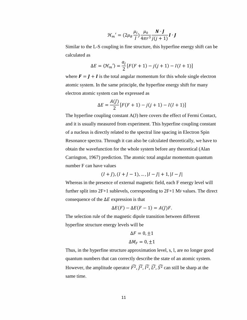
Similar to the L-S coupling in fine structure, this hyperfine energy shift can be

calculated as

⟨ ⟩

[ ]

where is the total angular momentum for this whole single electron

atomic system. In the same principle, the hyperfine energy shift for many

electron atomic system can be expressed as

[ ]

The hyperfine coupling constant A(J) here covers the effect of Fermi Contact,

and it is usually measured from experiment. This hyperfine coupling constant

of a nucleus is directly related to the spectral line spacing in Electron Spin

Resonance spectra. Through it can also be calculated theoretically, we have to

obtain the wavefunction for the whole system before any theoretical (Alan

Carrington, 1967) prediction. The atomic total angular momentum quantum

number F can have values

Whereas in the presence of external magnetic field, each F energy level will

further split into 2F+1 sublevels, corresponding to 2F+1 MF values. The direct

consequence of the expression is that

.

The selection rule of the magnetic dipole transition between different

hyperfine structure energy levels will be

Thus, in the hyperfine structure approximation level, s, l, are no longer good

quantum numbers that can correctly describe the state of an atomic system.

However, the amplitude operator can still be sharp at the

same time.

12

2.3.2. Atomic electric quadrupole hyperfine structure

Some nuclei with spins of 1 or more also possess an electric quadrupole

moment with occurs because the distribution of electric charge density

inside the nucleus is ellipsoidal rather than spherical (Alan Carrington,

1967). It is defined by

∫

Here the z direction is parallel to the spin vector I and the integral extends

over the interior of the nucleus. If an electric field gradient exist at the nucleus,

an electric quadrupole hyperfine coupling will introduce an additional energy

level split. Quantum mechanics calculations show that the energy shift due to

nuclear electric quadrupole hyperfine coupling can be represented as

Where , and ⟨

⟩ (Yang, 2004).

Q is the electric quadrupole of the nucleus and ⟨

⟩ is the expectation value

of the electric field gradient due to extranuclear electrons, which depends on

specific electron wave functions. It should be noted that in the following three

cases, the electric quadrupole coupling does not exist. (1) For the spherically

symmetric distribution of s orbital electrons, their ⟨

⟩ at r=0. (2) When

the total nuclear spin angular momentum I=0 or ½, Q=0. (3) For electrons

with total angular momentum of J=0 or ½, their ⟨

⟩ at r=0. Except for

those three cases mentioned above, the hyperfine coupling energy shifts are

always the superposition of magnetic dipole and electric quadrupole

components, which can be written in a general form (Yang, 2004)

2.3.3. Molecular hyperfine structure

The molecular hyperfine Hamiltonian includes those terms already derived for

the atomic case with a magnetic dipole term for each nucleus with I>0 and an

electric quadrupole term for each nucleus with I>1. In addition to the effects

13

described above there are a number of effects specific to the molecular case.

For example, direct nuclear spin-spin coupling occurs for each nucleus with

I>0 due to the presence of the combined field of all of the other nuclear

magnetic moments in a molecule. A summation over each magnetic moment

dotted with the field due to each other magnetic moment gives the direct

nuclear spin-spin term in the hyperfine Hamiltonian

∑

where a and a’ are indices representing the nucleus contributing to the energy

and the nucleus that is the source of the field respectively (Alan Carrington,

1967). Another example of molecular hyperfine component will be the

nuclear spin-rotation hyperfine coupling where the nuclear magnetic

momentum in a molecule obtains extra energy in a magnetic field component

due to the angular momentum associated with the bulk rotation of the

molecule. Such kinds of weak hyperfine coupling structures are numerous. It

is our application purpose that decides to which level of approximation we

should refer.

3. Electron Spin Resonance.

The principle idea behind any magnetic resonance are common for both electron spin

resonance and nuclear magnetic resonance, but there are differences in the magnitudes

and signs of the magnetic interactions involved, which naturally leads to divergence in

the experimental techniques employed.

If a molecule has one or more unpaired electrons, then this unpaired electron spin

magnetic moment will be the dominant contribution to the total magnetic moment.

Typical examples are free radicals and complexes possessing a transition metal ion. In

these cases, Electron Spin Resonance technique is used to study the molecular structure.

After deriving all the fantasy hyperfine structures in atoms and molecule, one may be

confused about why we get rid of that more comprehensive hyperfine structure model

and come back to Zeeman fine structure again in ESR practice. To explain the reason, let

14

us have a brief look of how ESP technique is used to decide molecular structures from g

factor.

3.1.EPR experiment

For an isolated electron, its magnetic moment and Hamiltonian under an applied

external magnetic field B (assuming B is along z direction) are

where is the gyromagnetic ratio for an isolated electron. The allowed component

of the electron spin in the z direction has value +1/2 or -1/2. In order to induce

transitions between the two electron spin levels, an oscillating electromagnetic field is

applied to the system. Absorption of energy occurs provided the magnetic vector of

the oscllating field is perpendicular to the steady field B and prvided the frequency v

of the oscillating field satisfies the resonance condition,

This equation indicates that one could look for a nuclear resonance absorption by

varying either the magnetic field B or the frequency v. In practice, one usually works

with a fixed frequency v, sweeping the magnetic field through the resonance value

and obtain a spectrum in which the absorption of the energy is plotted as a function of

the magnetic field strength. Since in terms of gyromagnetic ratio and angular

frequency, the Hamiltonian can be written as

In fact, the unpaired electron in molecule is not isolated. The spectrometer’s applied

resonance magnetic field in resonance condition must be replaced by an effective

field whose value is slightly different from B and varies according to the chemical

environment of the electron. The effective field experienced by the electron is

thus written as , where includes the effect of local environment

and can be either positive or negative. Thus the resonance condition can be rewritten

as

15

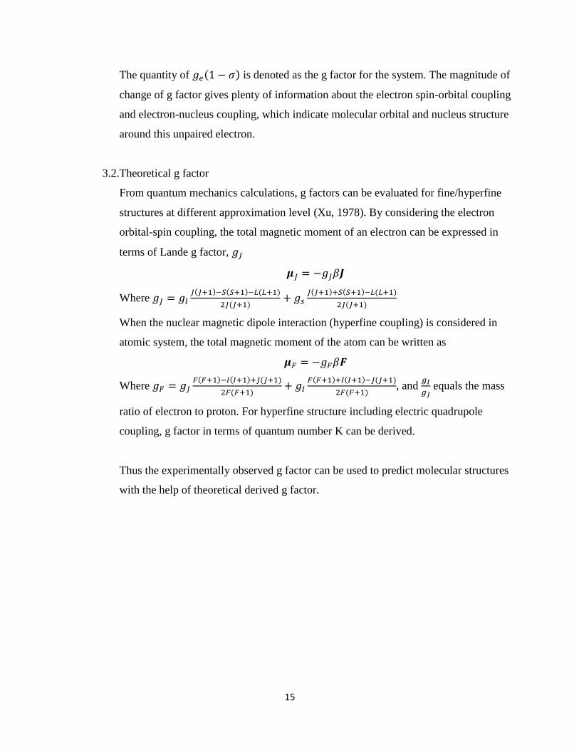
The quantity of is denoted as the g factor for the system. The magnitude of

change of g factor gives plenty of information about the electron spin-orbital coupling

and electron-nucleus coupling, which indicate molecular orbital and nucleus structure

around this unpaired electron.

3.2.Theoretical g factor

From quantum mechanics calculations, g factors can be evaluated for fine/hyperfine

structures at different approximation level (Xu, 1978). By considering the electron

orbital-spin coupling, the total magnetic moment of an electron can be expressed in

terms of Lande g factor,

Where

When the nuclear magnetic dipole interaction (hyperfine coupling) is considered in

atomic system, the total magnetic moment of the atom can be written as

Where

, and

equals the mass

ratio of electron to proton. For hyperfine structure including electric quadrupole

coupling, g factor in terms of quantum number K can be derived.

Thus the experimentally observed g factor can be used to predict molecular structures

with the help of theoretical derived g factor.

16

Works Cited

Alan Carrington, A. D. (1967). Introduction to Magnetic Resonance. New York: Harper & Row.

Costella, J. P. (1994). Single-Particle Electrodynamics. Melbourne: University of Melbourne.

John A. Weil, J. R. (2007). Electron Paramagnetic Resonance-Elementary Theory and Practical

Applications. Hoboken, New Jersey: Wiley-Interscience.

R. Neugart, G. N. (2005). Nuclear Moments. Mainz, Germany.

Xu, G. (1978). Electron Paramagnetic Resonance Spectrum Principle. Beijing: The Commercial Press.

Yang, J. (2004). Atomic Physics. Beijing: Higher Education Press.