1  

Measuring the Hyperfine Levels of Rubidium Using Saturated Absorption Spectroscopy

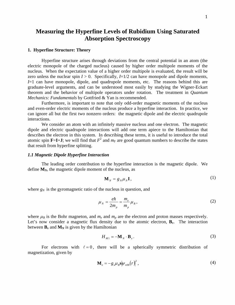
1. Hyperfine Structure: Theory Hyperfine structure arises through deviations from the central potential in an atom (the electric monopole of the charged nucleus) caused by higher order multipole moments of the nucleus. When the expectation value of a higher order multipole is evaluated, the result will be zero unless the nuclear spin I > 0. Specifically, I=1/2 can have monopole and dipole moments, I=1 can have monopole, dipole, and quadrupole moments, etc. The reasons behind this are graduate-level arguments, and can be understood most easily by studying the Wigner-Eckart theorem and the behavior of multipole operators under rotation. The treatment in Quantum Mechanics: Fundamentals by Gottfried & Yan is recommended. Furthermore, is important to note that only odd-order magnetic moments of the nucleus and even-order electric moments of the nucleus produce a hyperfine interaction. In practice, we can ignore all but the first two nonzero orders: the magnetic dipole and the electric quadrupole interactions.

We consider an atom with an infinitely massive nucleus and one electron. The magnetic dipole and electric quadrupole interactions will add one term apiece to the Hamiltonian that describes the electron in this system. In describing these terms, it is useful to introduce the total atomic spin F=I+J; we will find that F2 and mF are good quantum numbers to describe the states that result from hyperfine splitting.

1.1 Magnetic Dipole Hyperfine Interaction

The leading order contribution to the hyperfine interaction is the magnetic dipole. We define MN, the magnetic dipole moment of the nucleus, as

IM NNN g μ= ,

where gN is the gyromagnetic ratio of the nucleus in question, and

Bp

e

pN m

mme μμ ==

2h ,

where μB is the Bohr magneton, and me and mp are the electron and proton masses respectively. Let’s now consider a magnetic flux density due to the atomic electron, Be. The interaction between Be and MN is given by the Hamiltonian

eNMH BM ⋅−=1 .

For electrons with 0=l , there will be a spherically symmetric distribution of magnetization, given by

( )200 rg nBse ψμ sM −= ,

(1)

(2)

(3)

(4)

2  

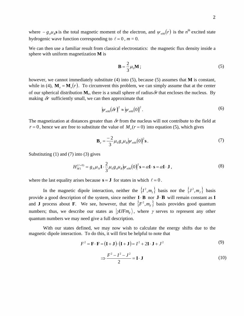
where sBsg μ− is the total magnetic moment of the electron, and ( )rn00ψ is the nth excited state hydrogenic wave function corresponding to 0=l , m = 0.

We can then use a familiar result from classical electrostatics: the magnetic flux density inside a sphere with uniform magnetization M is

MB 032 μ= ; 

however, we cannot immediately substitute (4) into (5), because (5) assumes that M is constant, while in (4), ( )ree MM = . To circumvent this problem, we can simply assume that at the center of our spherical distribution Me, there is a small sphere of radius rδ that encloses the nucleus. By making rδ sufficiently small, we can then approximate that

( ) ( )200

200 0nn r ψδψ ≈ .

The magnetization at distances greater than rδ from the nucleus will not contribute to the field at 0=r , hence we are free to substitute the value of )0( =rMe into equation (5), which gives

( ) sB 2000 0

32

nBse g ψμμ−= .

Substituting (1) and (7) into (3) gives

( ) JIsIsI ⋅=⋅=⋅== ααψμμμ 2000

)0(1 0

32

nBsNNM ggH l ,

where the last equality arises because Js = for states in which 0=l .

In the magnetic dipole interaction, neither the { }ImI ,2 basis nor the { }JmJ ,2 basis provide a good description of the system, since neither BI ⋅ nor BJ ⋅ will remain constant as I and J process about F. We see, however, that the { }FmF ,2 basis provides good quantum numbers; thus, we describe our states as FIJFmγ , where γ serves to represent any other quantum numbers we may need give a full description.

With our states defined, we may now wish to calculate the energy shifts due to the magnetic dipole interaction. To do this, it will first be helpful to note that

( ) ( ) 222 2 JIF +⋅+=+⋅+=⋅= JIJIJIFF

JI ⋅=−−

⇒2

222 JIF

(5)

(6)

(7)

(8)

(9)

(10)

3  

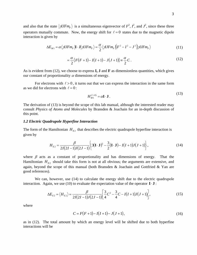
and also that the state FIJFmγ is a simultaneous eigenvector of F2, I2, and J2, since these three operators mutually commute. Now, the energy shift for 0=l states due to the magnetic dipole interaction is given by

( ) FFFFM IJFmJIFIJFmIJFmIJFmE γγαγγα 2221 2

−−=⋅=Δ JI

( ) ( ) ( ){ } CJJIIFF2

1112

αα≡+−+−+= .

As is evident from (12), we choose to express I, J and F as dimensionless quantities, which gives our constant of proportionality α dimensions of energy.

For electrons with 0>l , it turns out that we can express the interaction in the same form as we did for electrons with 0=l :

JI ⋅=> α)0(1l

MH .

The derivation of (13) is beyond the scope of this lab manual, although the interested reader may consult Physics of Atoms and Molecules by Bransden & Joachain for an in-depth discussion of this point.

1.2 Electric Quadrupole Hyperfine Interaction

The form of the Hamiltonian 2EH that describes the electric quadrupole hyperfine interaction is given by

( ) ( ) ( ) ( ) ( ) ( )⎭⎬⎫

⎩⎨⎧ ++−⋅−⋅

−−= 11

233

121222

2 JJIIJJII

HE JIJIβ ,

where β acts as a constant of proportionality and has dimensions of energy. That the Hamiltonian 2EH should take this form is not at all obvious; the arguments are extensive, and again, beyond the scope of this manual (both Bransden & Joachain and Gottfried & Yan are good references).

We can, however, use (14) to calculate the energy shift due to the electric quadrupole interaction. Again, we use (10) to evaluate the expectation value of the operator JI ⋅ :

( ) ( ) ( ) ( )⎥⎦⎤

⎢⎣⎡ ++−−

−−==Δ 11

43

43

121222

22 JJIICCJJII

HE EEβ ,

where

( ) ( ) ( )111 +−+−+= JJIIFFC ,

as in (12). The total amount by which an energy level will be shifted due to both hyperfine interactions will be

(11)

(12)

(13)

(14)

(15)

(16)

4  

21 EMhfs EEE Δ+Δ=Δ ,

where the subscript hfs denotes hyperfine structure.

1.3 Hyperfine Structure of Rubidium

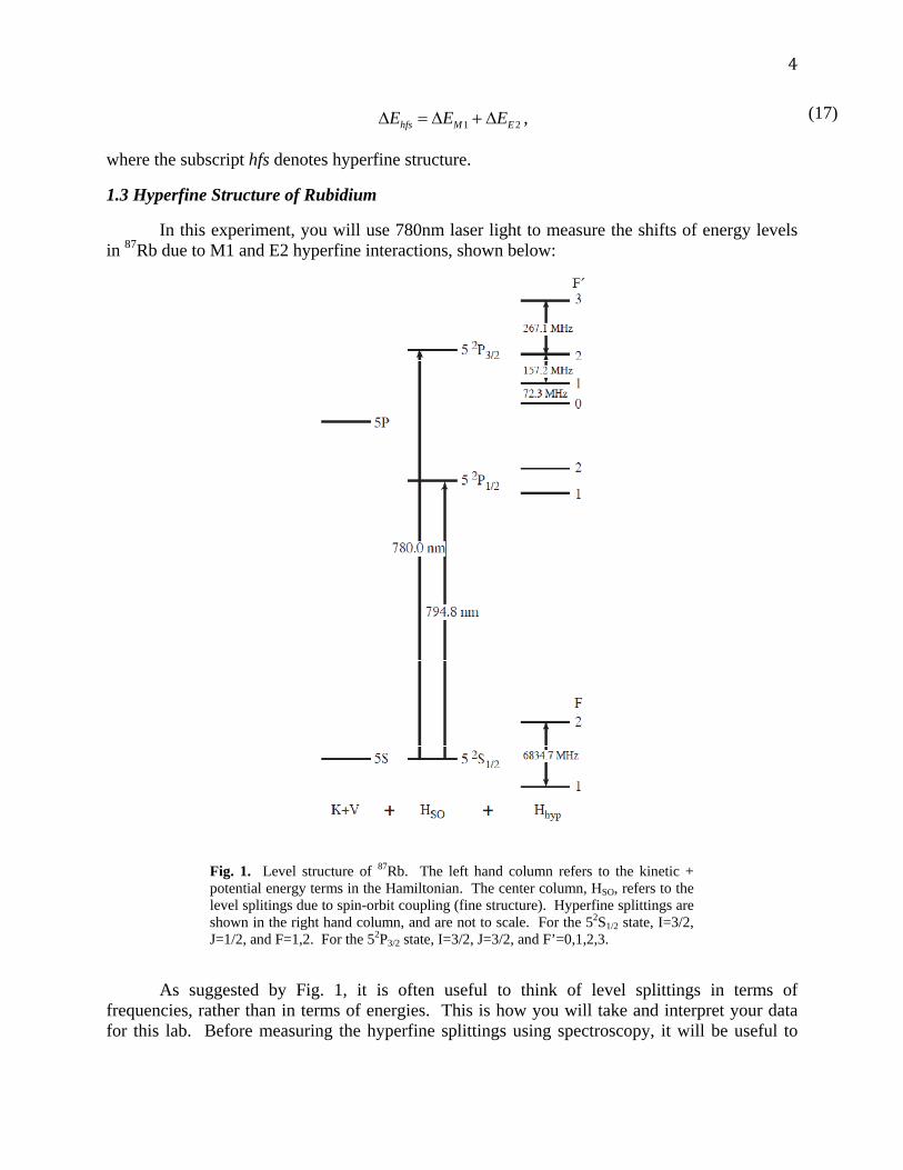
In this experiment, you will use 780nm laser light to measure the shifts of energy levels in 87Rb due to M1 and E2 hyperfine interactions, shown below:

As suggested by Fig. 1, it is often useful to think of level splittings in terms of frequencies, rather than in terms of energies. This is how you will take and interpret your data for this lab. Before measuring the hyperfine splittings using spectroscopy, it will be useful to

(17)

Fig. 1. Level structure of 87Rb. The left hand column refers to the kinetic + potential energy terms in the Hamiltonian. The center column, HSO, refers to the level splitings due to spin-orbit coupling (fine structure). Hyperfine splittings are shown in the right hand column, and are not to scale. For the 52S1/2 state, I=3/2, J=1/2, and F=1,2. For the 52P3/2 state, I=3/2, J=3/2, and F’=0,1,2,3.

5  

calculate them using the theory that was just discussed. We already know that the energy shift due to the hyperfine interaction is given by

( ) ( ) ( ) ( )⎥⎦⎤

⎢⎣⎡ ++−+

−−+=Δ+Δ=Δ 11

43

43

1212222

21 JJIICCJJII

CEEE EMhfsβα .

To see how this equation correlates with our level splittings in Fig. 1, we divide (18) by Planck’s constant h, and the resulting frequency shifts of a level due to the hyperfine interaction is given by

( ) ( ) ( ) ( ) ( )⎥⎦⎤

⎢⎣⎡ ++−+

−−+=Δ 111

43

121222JJIICC

JJIIBCAhfsν ,

where A and B have units of hertz. For the two states in question, the 52S1/2 state and the 52P3/2 state in 87Rb, the accepted values of A and B have been experimentally determined. The 52S1/2 state has A = 3417.34 MHz (the term that multiplies B in (19) reduces to zero for this state), and the 52P3/2 state has A = 84.72 MHz and B = 12.50 MHz.

2. Saturated Absorption Spectroscopy: Theory

2.1 Doppler Broadening

The atoms in the rubidium cell constitute a gas at room temperature, and thus they are undergoing random thermal motion. If the laser is propagating along the z-axis, and the velocity of the atom has a nonzero component in the z-direction, then the frequency of the radiation absorbed by the atom is given by

⎟⎠⎞

⎜⎝⎛ +=

cVz

L 10νν ,

where 0ν is the resonant absorption frequency for an atom at rest, and zV is the z-component of the atom’s velocity. Keeping in mind that the positive z-axis points along the direction of laser propagation, we see that atoms moving towards the laser ( 0<zV ) will resonantly absorb radiation 0νν <L . The radiation Lν is blue-shifted up to 0ν due to the Doppler effect. A similar conclusion can be drawn for atoms moving away from the laser. Because the rubidium cell consists of many atoms undergoing random thermal motion, there will be a distribution of zVvalues, and a wider range of laser frequencies will be absorbed. This effect, which tends to mask the more subtle features of absorption spectra (such as hyperfine structure) is known as Doppler broadening.

We assume a Maxwell distribution of velocities of the atoms in the cell, and again examine only the z-component of the atomic velocities. The probability that an atom’s velocity is between zV and zz dVV + is given by

( ) zB

z

Bzz dV

TkMV

TkMdVVP ⎥

⎦

⎤⎢⎣

⎡−⋅=

2exp

2

2

π,

(18)

(19)

(20)

(21)

6  

where M is the atom’s mass, Bk is the Boltzmann constant, and T is temperature.

Solving (20) for zV and taking the differential, we find that

Lz dcdV νν 0

= .

Substituting (22) into (21), we find that the probability for an atom to absorb a photon between frequency Lν and LL dνν + is given by

( ) ( )L

LLL ddP ν

δνν

πδνν ⎥

⎦

⎤⎢⎣

⎡ −−⋅= 2

204exp2 ,

where

MTk

cB22 0νδ = .

Notice that (23) describes a Gaussian probability distribution centered at 0ν , with a full width at half maximum (FWHM) given by

( ) ( )MT

MTk

cB

0200

2/1 1092.22ln222ln ννδν −×≈==Δ .

2.2 Saturated Absorption Spectroscopy

Saturated absorption spectroscopy uses two counter propagating beams at the same frequency interacting with the same group of atoms. This configuration produces an absorption signal that contains features ordinarily masked by Doppler broadening.

(22)

(23)

(24)

(25)

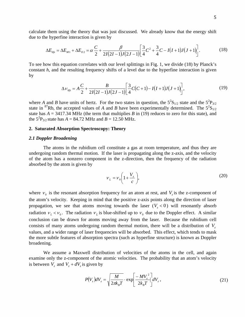
Fig. 2. Optical setup for saturated absorption spectroscopy. The labels and optical components are fully explained in section 3. Here, note that a portion of the beam is deflected by the polarizing beam splitter (PBS), passes through the rubidium cell (Rb), is reflected backwards by a mirror (M2), passes through the cell again, and finally hits a detector (D1). The beam’s first pass through the cell acts as a pump, and the beam’s second pass through the cell acts as a probe.

7  

As shown in Fig. 2, the beam passes twice through the cell. On its first pass, if the beam is not at frequency 0ν , then it will interact with atoms whose z-component of velocity is Vz , where Vz is given by (20). After the beam has been reflected, and is travelling back through cell, it will interact with atoms whose z-component of velocity is –Vz , since the beam is now propagating in the opposite direction. Notice that when the beam is off resonance, it interacts with two different groups of atoms.

When the beam is on resonance (at frequency 0ν ), however, it will interact with atoms that have zero velocity along the z-axis on both passes through the cell. This is the heart of saturation spectroscopy. We call the first pass through the cell the pump beam, because it will excite a transition in atoms with 0=zV , pumping them out of the ground state. As the beam passes back through the cell, it functions as the probe beam, because it is the absorption of this beam that eventually gets detected. When the laser is on resonance with the 0=zV atoms, there is a sharp decrease in absorption (seen as a sharp increase in the signal from the detector), since many of these atoms have been pumped out of the ground state, and will not be able to absorb any photons from the resonant probe beam. Note that this only happens because the pump and probe are interacting with the same group of atoms: those with 0=zV . If the laser is off resonance, this feature is not present, and the spectrum will not contain sub-Doppler features.

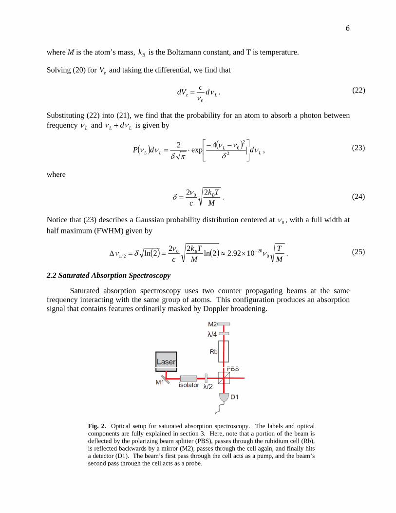
If the frequency of the laser is oscillating, so that it sweeps through the frequency 0ν , then we expect to see a Doppler broadened absorption signal, with sharp increases “riding” on top of the signal, which correspond to hyperfine transitions. Consider for example the F=2 ground state of 87Rb. Without using a pump beam, one would see a Doppler broadened signal that contains little or no signature of the three separate hyperfine transitions corresponding to F’=1, F’=2, and F’=3. When a pump and probe beam are both used, however, the signal will acquire sub-Doppler features corresponding to the three hyperfine transitions.

Fig. 3. (a) Spectroscopy of Rubidium using only a probe beam. Sub-Doppler features are not resolved. (b) Saturated absorption spectroscopy. The sharp peaks “riding” on the Doppler-broadened absorption signal correspond to hyperfine transitions.

8  

2.3 Crossover Resonances

There is a peculiar feature of saturated absorption spectroscopy that you will observe when taking data: in addition to the sharp increases in signal corresponding to the points at which the laser is resonant with a hyperfine transition, there will be sharp increases corresponding to points at which the laser frequency is halfway between two different hyperfine transitions. When this occurs, it is known as a crossover transition or crossover resonance. A discussion of why this occurs is outside the scope of this manual, although chapter 8 of Atomic Physics by C. J. Foot is a good reference for the interested reader.

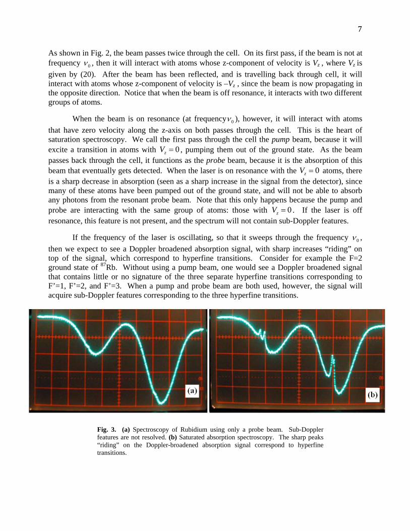
Again, consider the example of the F=2 ground state in 87Rb. There are three hyperfine transitions at frequencies 1ν , 2ν , and 3ν corresponding to F’=1, F’=2, and F’=3. Hence there are three crossover resonances: ( ) 2/21 νν + , ( ) 2/32 νν + , and ( ) 2/31 νν + .

It is important to note that in practice, crossover resonances are often much stronger than the resonances corresponding to the ordinary hyperfine transitions. When taking data, you’ll probably only be able to see crossover resonances. Keep this in mind when using your data to calculate the hyperfine splittings in rubidium.

Fig. 4. Hyperfine structure of 87Rb, with crossover resonances shown. Transitions a, c, f, g, i, and l correspond to ordinary hyperfine transitions; b, d, e, h, j, and k correspond to crossover resonances. Note that some of the crossover resonances are not quite drawn to scale.

9  

3. Rubidium Saturated Absorption Spectroscopy: Experiment

3.1 Instrumental Setup

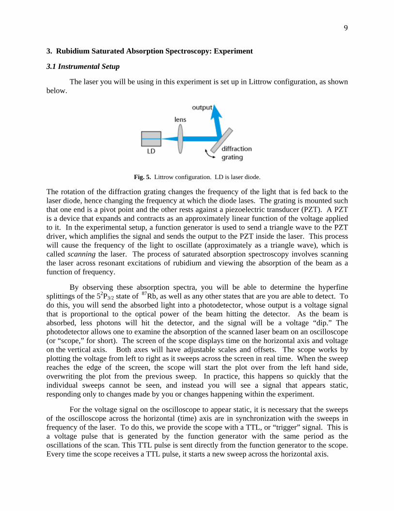
The laser you will be using in this experiment is set up in Littrow configuration, as shown below.

Fig. 5. Littrow configuration. LD is laser diode.

The rotation of the diffraction grating changes the frequency of the light that is fed back to the laser diode, hence changing the frequency at which the diode lases. The grating is mounted such that one end is a pivot point and the other rests against a piezoelectric transducer (PZT). A PZT is a device that expands and contracts as an approximately linear function of the voltage applied to it. In the experimental setup, a function generator is used to send a triangle wave to the PZT driver, which amplifies the signal and sends the output to the PZT inside the laser. This process will cause the frequency of the light to oscillate (approximately as a triangle wave), which is called scanning the laser. The process of saturated absorption spectroscopy involves scanning the laser across resonant excitations of rubidium and viewing the absorption of the beam as a function of frequency.

By observing these absorption spectra, you will be able to determine the hyperfine splittings of the 52P3/2 state of 87Rb, as well as any other states that are you are able to detect. To do this, you will send the absorbed light into a photodetector, whose output is a voltage signal that is proportional to the optical power of the beam hitting the detector. As the beam is absorbed, less photons will hit the detector, and the signal will be a voltage “dip.” The photodetector allows one to examine the absorption of the scanned laser beam on an oscilloscope (or “scope,” for short). The screen of the scope displays time on the horizontal axis and voltage on the vertical axis. Both axes will have adjustable scales and offsets. The scope works by plotting the voltage from left to right as it sweeps across the screen in real time. When the sweep reaches the edge of the screen, the scope will start the plot over from the left hand side, overwriting the plot from the previous sweep. In practice, this happens so quickly that the individual sweeps cannot be seen, and instead you will see a signal that appears static, responding only to changes made by you or changes happening within the experiment.

For the voltage signal on the oscilloscope to appear static, it is necessary that the sweeps of the oscilloscope across the horizontal (time) axis are in synchronization with the sweeps in frequency of the laser. To do this, we provide the scope with a TTL, or “trigger” signal. This is a voltage pulse that is generated by the function generator with the same period as the oscillations of the scan. This TTL pulse is sent directly from the function generator to the scope. Every time the scope receives a TTL pulse, it starts a new sweep across the horizontal axis.

10  

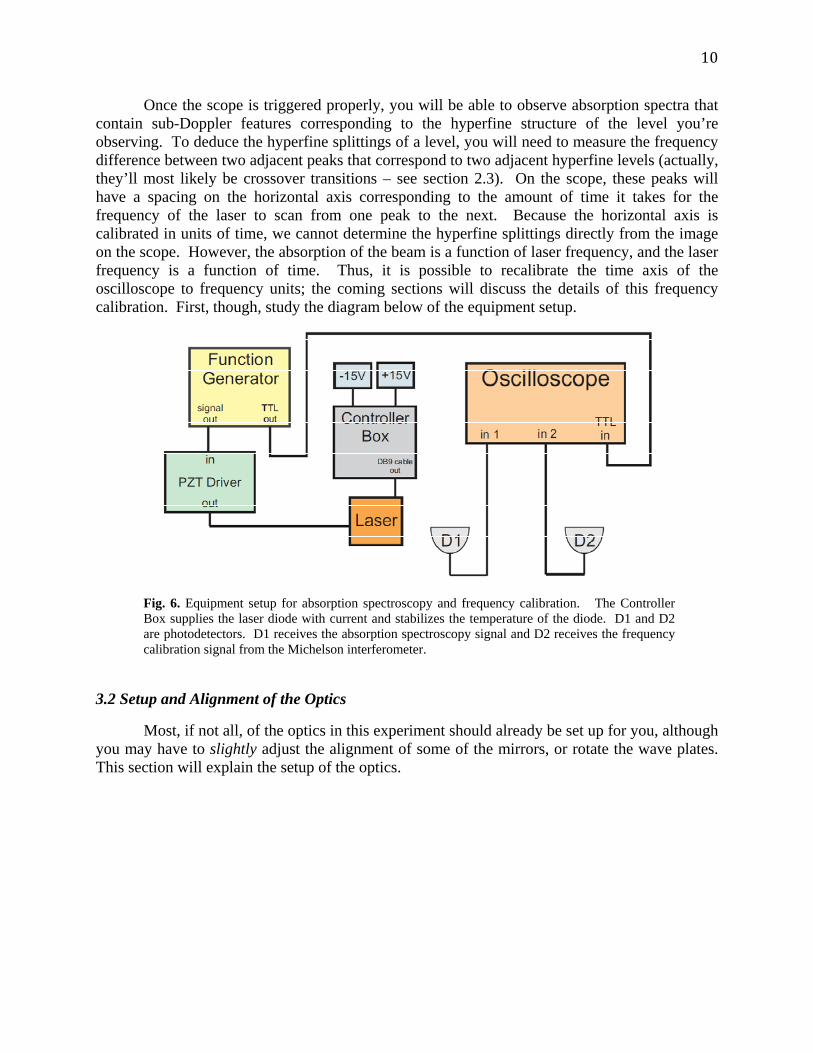
Once the scope is triggered properly, you will be able to observe absorption spectra that contain sub-Doppler features corresponding to the hyperfine structure of the level you’re observing. To deduce the hyperfine splittings of a level, you will need to measure the frequency difference between two adjacent peaks that correspond to two adjacent hyperfine levels (actually, they’ll most likely be crossover transitions – see section 2.3). On the scope, these peaks will have a spacing on the horizontal axis corresponding to the amount of time it takes for the frequency of the laser to scan from one peak to the next. Because the horizontal axis is calibrated in units of time, we cannot determine the hyperfine splittings directly from the image on the scope. However, the absorption of the beam is a function of laser frequency, and the laser frequency is a function of time. Thus, it is possible to recalibrate the time axis of the oscilloscope to frequency units; the coming sections will discuss the details of this frequency calibration. First, though, study the diagram below of the equipment setup.

3.2 Setup and Alignment of the Optics

Most, if not all, of the optics in this experiment should already be set up for you, although you may have to slightly adjust the alignment of some of the mirrors, or rotate the wave plates. This section will explain the setup of the optics.

Fig. 6. Equipment setup for absorption spectroscopy and frequency calibration. The Controller Box supplies the laser diode with current and stabilizes the temperature of the diode. D1 and D2 are photodetectors. D1 receives the absorption spectroscopy signal and D2 receives the frequency calibration signal from the Michelson interferometer.

11  

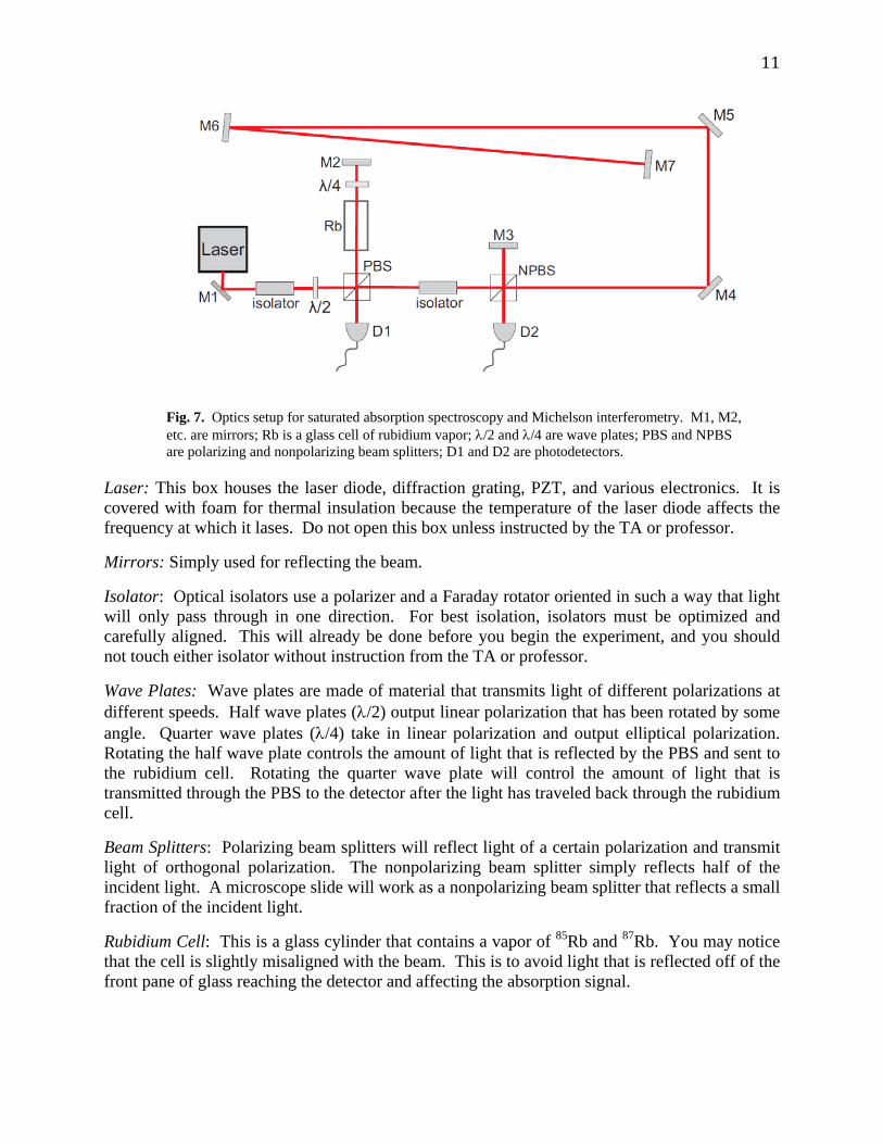
Laser: This box houses the laser diode, diffraction grating, PZT, and various electronics. It is covered with foam for thermal insulation because the temperature of the laser diode affects the frequency at which it lases. Do not open this box unless instructed by the TA or professor.

Mirrors: Simply used for reflecting the beam.

Isolator: Optical isolators use a polarizer and a Faraday rotator oriented in such a way that light will only pass through in one direction. For best isolation, isolators must be optimized and carefully aligned. This will already be done before you begin the experiment, and you should not touch either isolator without instruction from the TA or professor.

Wave Plates: Wave plates are made of material that transmits light of different polarizations at different speeds. Half wave plates (λ/2) output linear polarization that has been rotated by some angle. Quarter wave plates (λ/4) take in linear polarization and output elliptical polarization. Rotating the half wave plate controls the amount of light that is reflected by the PBS and sent to the rubidium cell. Rotating the quarter wave plate will control the amount of light that is transmitted through the PBS to the detector after the light has traveled back through the rubidium cell.

Beam Splitters: Polarizing beam splitters will reflect light of a certain polarization and transmit light of orthogonal polarization. The nonpolarizing beam splitter simply reflects half of the incident light. A microscope slide will work as a nonpolarizing beam splitter that reflects a small fraction of the incident light.

Rubidium Cell: This is a glass cylinder that contains a vapor of 85Rb and 87Rb. You may notice that the cell is slightly misaligned with the beam. This is to avoid light that is reflected off of the front pane of glass reaching the detector and affecting the absorption signal.

Fig. 7. Optics setup for saturated absorption spectroscopy and Michelson interferometry. M1, M2, etc. are mirrors; Rb is a glass cell of rubidium vapor; λ/2 and λ/4 are wave plates; PBS and NPBS are polarizing and nonpolarizing beam splitters; D1 and D2 are photodetectors.

12  

Photodetectors: These detectors contain photodiodes whose output is a voltage signal proportional to the optical power of the beam hitting the detector.

The first section of the optics setup is used for saturated absorption spectroscopy. The half wave plate is rotated to control the power of the beam that will be reflected by the PBS. This portion of the beam then travels through the rubidium cell, a quarter wave plate, and is retroreflected. After the beam has passed twice through the rubidium cell, a portion of it will be transmitted through the PBS and reach the detector. Rotating the quarter wave plate will maximize the amount of light that reaches the detector, although this should already be done before you start the lab.

The portion of the beam that is not reflected by the PBS will be transmitted, pass through the second isolator, and be used to create an interferometry signal. This is the signal that will be used to calibrate the horizontal axis on the oscilloscope in units of frequency, rather than time.

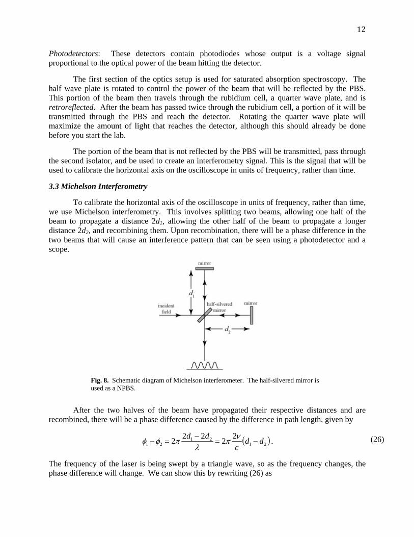
3.3 Michelson Interferometry

To calibrate the horizontal axis of the oscilloscope in units of frequency, rather than time, we use Michelson interferometry. This involves splitting two beams, allowing one half of the beam to propagate a distance 2d1, allowing the other half of the beam to propagate a longer distance 2d2, and recombining them. Upon recombination, there will be a phase difference in the two beams that will cause an interference pattern that can be seen using a photodetector and a scope.

After the two halves of the beam have propagated their respective distances and are recombined, there will be a phase difference caused by the difference in path length, given by

( )2121

2122222 ddc

dd−=

−=−

νπλ

πφφ .

The frequency of the laser is being swept by a triangle wave, so as the frequency changes, the phase difference will change. We can show this by rewriting (26) as

Fig. 8. Schematic diagram of Michelson interferometer. The half-silvered mirror is used as a NPBS.

(26)

13  

( )214 ddc

−Δ

=Δνπφ .

At the detector, the voltage signal will be proportional to the intensity of the beam hitting the detector, which will be given (up to a constant) by

⎟⎟⎠

⎞⎜⎜⎝

⎛+⎟

⎟⎠

⎞⎜⎜⎝

⎛+=∝

⎟⎠⎞

⎜⎝⎛ −−⎟

⎠⎞

⎜⎝⎛ −−⎟

⎠⎞

⎜⎝⎛ −⎟

⎠⎞

⎜⎝⎛ − tditditditdi

eEeEeEeEEEIπν

λππν

λππν

λππν

λπ 222

2

222

1

222

2

222

1*

2121

( )φΔ++= cos2 2*

12

22

1 EEEE

The interference will reach a maximum when πφ 2=Δ . Hence, the frequency of spacing of the interference maxima will be given by

( )212 ddc−

=Δν .

It is the spacing of the interference maxima that will be used as a frequency calibration for the horizontal axis on the oscilloscope.

3.4 Experimental Procedure

1. Ensure that the +/- 15V power supplies are connected to the appropriate places on the controller box (there will be labels on the box to guide you), and that the DB9 cable is connecting the controller box to the laser. At no point during the experiment should this cable be disconnected. The current to the laser diode runs through this cable, and an abrupt drop in current could ruin the diode.

2. Without turning the controller box on, check to see that the current control knob (lower left-hand position on the front panel of the controller box) is turned to its most counterclockwise position.

3. Turn the controller box on, and flip the switch labeled “current” to its up position.

4. Turn on the temperature stabilization by flipping the two switches on the controller box located between the two sets of LEDs to their up position. After about five minutes, the electronics inside the controller box will have thermally stabilized the laser, which will keep the frequency of the laser from drifting.

5. As you know, the laser emits light at 780 nm, which is in the infrared and is barely visible. An IR card should be provided so that you can locate and trace the beam. Hold the surface of the IR card in the path of the beam (which has not yet been turned on), and watch for the beam to appear on the card as you turn the “current” knob on the controller box clockwise. This provides the diode with current, and it should begin to lase. The controller box limits the amount of current that will go to the diode, so there’s no harm in turning the knob up most of the way, so the beam is easier to see on the card. Eventually, you will adjust the current on the controller

(27)

(30)

(28)

(29)

14  

box to tune the frequency of the laser, at which point you will probably have to turn the current down to see the absorption spectra.

6. Using the IR card, trace the path of the beam through the saturation spectroscopy portion of the optical setup. Try holding the card just before the rubidium cell and rotating the half wave plate to observe the effects. Rotate the half wave plate so that the beam is visible on the card. Then, hold the card at D1 (referring to Fig. 7) and ensure that the beam is hitting the photodiode on the detector. If no beam is visible, try rotating the quarter wave plate. If you still cannot see a beam hitting the detector, ask your TA or professor. The alignment of optics is very sensitive; take care not to bump any of the optics with your hand while making adjustments to the waveplates.

7. Make sure the detector D1 is plugged into its power supply, and the power supply is plugged into the wall (this should already be done for you). Turn the detector on using the switch on the back. Then, connect the detector to channel 1 of the oscilloscope. Set the scope to “DC coupling.” Analog scopes: There will be a switch on the front panel of the scope that switches the channel from AC coupling to DC coupling to ground. Select “DC coupling.” Digital scopes: Press the button near the input for channel 1 that is simply labeled “Channel 1.” On the screen, to the right of the trace, will be a column of options. Press the button next to the option entitled “coupling” to toggle between AC and DC coupling. If you cannot see a trace on the scope (which at this point will be a horizontal line), try adjusting the “VOLTS/DIV” knob corresponding to channel 1 on the scope. This will adjust the scale of the vertical axis on the scope.

8. Try rotating the quarter wave plate, which will change the power of the light that is reaching the detector, and viewing the effects of the voltage signal on the scope. If no effect is present, and your trace is not at ground, try reducing the volts/div of the vertical axis. If this causes the trace to disappear from the screen, you can bring it back by adjusting the vertical offset of channel 1 using the “position” or “vertical position” knob on the scope corresponding to channel 1. Rotate the quarter wave plate until the voltage on scope is maximized. This will maximize the amount of light that is being transmitted from the rubidium, through the PBS, and to the detector. Additionally, you could try rotating the two knobs on the back of the mount of the retroreflection mirror (M2) to optimize the signal. Mirror mounts are very sensitive, so it is recommended that you rotate these knobs slowly, and only if you are having problems with poor signal amplitude later on in the experiment.

9. Rotate the half wave plate until the voltage on the oscilloscope is minimized. This will minimize the amount of light that is reflected by the PBS and used for the saturation spectroscopy experiment. The reason we minimize the amount of light used is to avoid power broadening the absorption lines. If too much laser power is used to excite the transitions, the absorption lines will become broadened, and won’t be resolved as easily.

10. With the beam aligned and the wave plates optimized, you are ready to find the atomic transitions. To do this, you’ll need to scan the laser frequency. Connect the function generator to the PZT driver and to the scope as shown in Fig. 6. Now, set the scope to be triggered externally. Analog scopes: There will be a switch on the scope near the TTL input on the right-hand side of the scope’s front panel. The labeling varies from one scope to another, but it will probably say something like “EXT TRIG.” This is the correct setting, and tells the scope that you

15  

will be providing it with TTL pulses. Digital scopes: Press the button labeled “trigger menu” on the top right-hand corner of the scope’s front panel. This will bring up a column of options on the screen to the right of the trace. Press the button corresponding to the option labeled “source” to toggle between various settings. The option labeled “EXT” is the correct one.

11. Set the function generator to a triangle wave with a frequency of ~50Hz. Turn the knob that controls the amplitude of the signal towards the top of its range (turning it all the way up and backing off a little will be fine). Now, set the scope to AC coupling, in the same way that you adjusted the coupling before. There will be two BNC jacks mounted on the side of the laser box. Connect the PZT driver to the BNC jack that does not have a grounding cap on it.

12. The frequency of the laser is now being scanned. If you see a flat line on the scope, and everything is aligned and hooked up properly, it means the beam is not being absorbed. This is because the range of frequencies across which the beam is being swept does not overlap with the resonances of any atomic transitions. Change the frequency of the laser by slowly adjusting the current to the laser diode. (This is done by turning the “current” knob on the controller box in the same way that you did in step 5.) Once you are able to see features of absorption on the scope, stop adjusting the current.

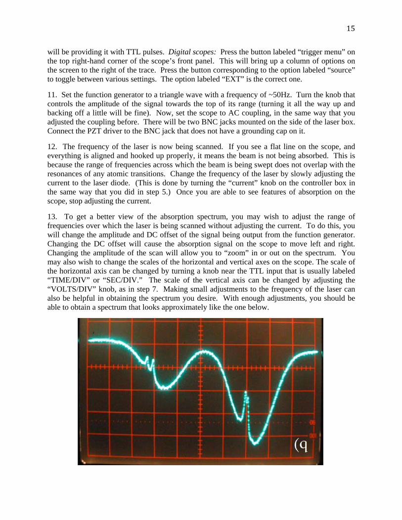
13. To get a better view of the absorption spectrum, you may wish to adjust the range of frequencies over which the laser is being scanned without adjusting the current. To do this, you will change the amplitude and DC offset of the signal being output from the function generator. Changing the DC offset will cause the absorption signal on the scope to move left and right. Changing the amplitude of the scan will allow you to “zoom” in or out on the spectrum. You may also wish to change the scales of the horizontal and vertical axes on the scope. The scale of the horizontal axis can be changed by turning a knob near the TTL input that is usually labeled “TIME/DIV” or “SEC/DIV.” The scale of the vertical axis can be changed by adjusting the “VOLTS/DIV” knob, as in step 7. Making small adjustments to the frequency of the laser can also be helpful in obtaining the spectrum you desire. With enough adjustments, you should be able to obtain a spectrum that looks approximately like the one below.

16  

14. Make sure the detector D2 is plugged into its power supply, and the power supply is plugged into the wall (this should already be done for you). Turn the detector on. Plug D2 into the second channel of the oscilloscope and use a note card or piece of paper to block D1. Make sure that channel 2 of the scope is on and is set to AC coupling. Analog scopes: There will be a 3-position switch, often between the controls for the two channels, with options for “ch 1,” “ch 2,” and “BOTH.” Flip the switch to the position corresponding to “BOTH.” Digital scopes: Pressing the button labeled “channel 2” above the input for channel 2 will toggle the channel on and off. The Michelson interferometer should already be aligned, but it’s a good idea to use the IR card to confirm that the beams are hitting the detector. Remember, the recombined beam must overlap at all points, not just at the detector.

15. Carefully measure the distances d1 and d2 and compute what the frequency spacing of the interference maxima will be.

16. On the scope, adjust the vertical position and scale of the channel 2 vertical axis until you obtain an oscillatory interference signal. Then, unblock D1 and view both signals on the same screen. Use the amplitude and DC offset of the function generator to “zoom in” on the 87Rb, F=2 absorption dip. Specifically, bring one crossover resonance peak to the left hand side of the screen, and an adjacent crossover resonance peak to the right hand side. Split them as far apart horizontally as you can. Count the number of Michelson interference maxima between the two crossover resonances and multiply this number by the frequency spacing calculated in step 15. This is an estimate of the frequency spacing of the two crossover resonance peaks in question. Digital scopes: Usually, the two channels will have independently adjustable horizontal axes. Make sure the time/div knob is on the same setting for both channels.

17. Because there are three crossover resonance peaks associated with the 87Rb, F=2 Doppler line, you will measure three frequency spacings: the spacing between the two leftmost crossover resonance peaks, the spacing between the two rightmost crossover resonance peaks, and the spacing between the leftmost and rightmost crossover resonance peaks. Record these spacings and use them to calculate the hyperfine splitting of the 5 2P3/2 level of 87Rb. Check to see that this agrees with theory. Repeating this step several times so that each member of the group takes several sets of data would be a good idea.

18. Because there will only be several interference maxima between hyperfine splittings, the resolution of the measurements will be low. For better frequency calibration, try viewing the output of the function generator on one channel of the scope, and viewing the signal from D2 on the other. Use the scope to measure the frequency difference in the laser as a function of volts put out by the function generator.

19. View the absorption signal on one channel of the scope and the output of the function generator on the other. Measure the difference in voltage that the function generator must sweep

Fig. 9. Partial saturated absorption spectrum of Rubidium vapor. The Doppler broadened absorption dip on the left corresponds to 87Rb, F=2. The three spikes in this absorption dip are due to the three crossover transitions that correspond to F=2 F’=1, F=2 F’=2, and F=2 F’=3. The Doppler broadened absorption dip on the right corresponds to 85Rb, F=3. When searching for absorption spectra, this feature is usually the most prominent and easiest to find.

17  

across to scan the laser across both crossover resonance peaks. Use this information to calculate the frequency difference in the crossover resonance peaks and then the hyperfine splittings of the 5 2P3/2 level. Comment on whether this method better agrees with theory.

20. Measure the FWHM of one of the Doppler-broadened lines. Use this measurement to estimate the mass of a rubidium atom, preferably in amu. It would be worthwhile to measure the room temperature, but approximating it as 298K will work if you don’t have a thermometer.

4. Discussion Topics

Explain why a triangle wave is used to scan the laser. What inherent assumption is being made about the frequency response of the laser as a function of output voltage from the function generator?

Why is it imperative that a NPBS (as opposed to a polarization-sensitive device) be used to split the beam at the Michelson interferometer? Why is polarization not an issue for the absorption spectroscopy portion of the experiment?

Explain why the method used in step 20 of the procedure is a crude approximation. Do you expect this method to underestimate or overestimate the mass of the rubidium atom?

5. References

Advanced discussions on hyperfine structure are found in Quantum Mechanics: Fundamentals by Gottfried and Yan, as well as Physics of Atoms and Molecules by Bransden and Joachain. The discussion in this manual is based on the arguments presented in Atomic Physics by C.J. Foot.

Atomic Physics also contains a thorough discussion of absorption spectroscopy, Doppler broadening, and sub-Doppler spectroscopic features at an introductory level. A more quantitative, advanced treatment can be found in Laser Spectroscopy: Basic Concepts and Instrumentation by W. Demtröder, Introduction to Nonlinear Laser Spectroscopy by M.D. Levenson, and others.

The experiment outlined in this lab manual is inspired by Doppler-Free Saturated Absorption Spectroscopy: Laser Spectroscopy, a lab manual used at the University of Colorado. It is not published at the time of this writing, but searching the title on Google will bring you to an online version.

18  

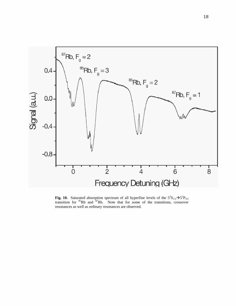
Fig. 10. Saturated absorption spectrum of all hyperfine levels of the 52S1/2 52P3/2 transition for 85Rb and 87Rb. Note that for some of the transitions, crossover resonances as well as ordinary resonances are observed.

19  

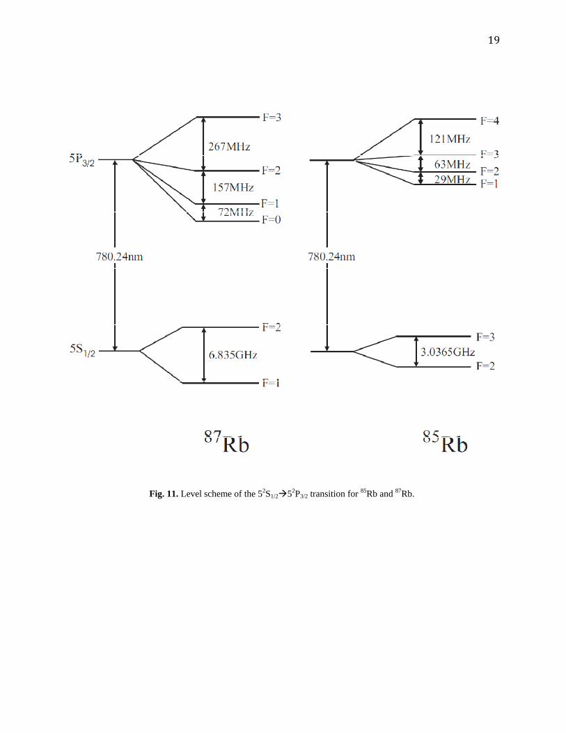
Fig. 11. Level scheme of the 52S1/2 52P3/2 transition for 85Rb and 87Rb.