AN INTRODUCTION TO FINITE ELEMENT METHODSuser.engineering.uiowa.edu/~kkchoi/Chapter_12.pdf552 Chap....

12

AN INTRODUCTION TO FINITE ELEMENT METHODS

As seen in Chapters 10 and 11, variational formulations of operator equations provide direct methods of constructing convergent numerical approximations to solutions of complex boundary-value problems. The Ritz method is particularly attractive for symmetric, positive bounded below operators that arise in nonhomogeneous equations and in eigenvalue problems. The principal limitation on the Ritz method is the construction of coordinate functions { cl>i(x) } for use in constructing approximations of the form

n

un(x) = L ai <1\(x) i=l

In practical applications, it is sometimes difficult to find coordinate functions in HA that are complete in energy and for which the Ritz equations are well posed. If the cPi(x) are linearly dependent, or if the Gram Determinant I [ <Pi• cpj ]A I is nearly zero, practical computational difficulties arise. The finite element method for constructing coordinate functions is introduced in this chapter, for use in variational solution of operator equations that arise in a wide variety of applications. The basic idea is to subdivide the underlying physical domain n into subsets ni• over which nonzero coordinate functions <Pi(x) are defined; i.e., cpj(x) = 0 on ni, for all j :;:. i. The result is a technique that systematically constructs coordinate functions that can be computer generated, even for irregularly shaped regions, and for which the resulting Ritz equations are computer generated and are well conditioned for numerical calculation. The development presented here is motivated by the elegant and more theoretically complete treatment of the subject by Strang and Fix [27]. The serious student of finite element methods is referred to Ref. 27 and related engineering books [6, 25, 28].

12.1 FINITE ELEMENTS FOR ONE DIMENSIONAL BOUNDARY-VALUE PROBLEMS

As an introduction, several finite elements are formulated for the Sturm-Liouville equation; e.g., for deflection of a string. In this one-dimensional problem, the construction of fmite elements is simple and natural. The equation

547

548 Chap. 12 An Introduction to Finite Element Methods

d ( du) - dx pCx) dx + q(x) u = fCx) C12.1.1)

for deflection of a string is first investigated. In order to illustrate the treatment of both principal and natural boundary conditions, the left end is fixed and the right end is free. Thus, at x = 0, there is a principal boundary condition

uCO) = 0 (12.1.2)

As shown in Section 11.1, the operator

d ( du) Au=- dX pCx) dx + q(x)u C12.1.3)

on the domain

D A = { u in C2(0, 1t): u(O) == u'(1t) = 0 } (12.1.4)

is positive bounded below if p(x) and q(x) are positive in (0, 1t). Therefore, from the Minimum Functional Theorem, the solution of the operator equation

Au= f (12.1.5)

is equivalent to finding a function in HA that minimizes

FCu) = fo'Jt [ p C u' )2 + qu2 - 2uf] dx C12.1.6)

Further, in Section 10.2, it was shown that the space HA consists of functions that have derivatives in 4CO, x). Thus, functions of the class D1(0, x) r1 cOco, 7t) are considered here.

To construct a finite element subspace sh of D1(0, x) n C°CO, x), the interval CO, 7t) is divided into segments of length h = x/n, on each of which the coordinate functions <!>f(x) are polynomials. Some degree of continuity is imposed at the boundaries between segments, but no more than is required in order that the following hold:

(1) The functions <!>f(x) are admissible in the variational principle. (2) Quantities of physical interest, usually displacements, stresses, or moments,

can be recovered from the approximate solution uh(x).

Linear Elements

In the string example, the admissible space is HA, whose members are continuous. This rules out piecewise constant functions. Therefore, the simplest choice for sh is the space of functions that are linear over each subinterval [ ( j- 1 ) h, jh ], continuous at the nodes x = jh, and zero at x = 0. The derivative of such a function is piecewise constant and obvi-

Sec. 12.1 Finite Elements for One Dimensional Boundary-Value Problems 549

ously has finite energy, so sh is a subspace ofHA. These coordinate functions are called linear finite elements, the subintervals are called finite elements (or simply elements), and the points jh are called nodes.

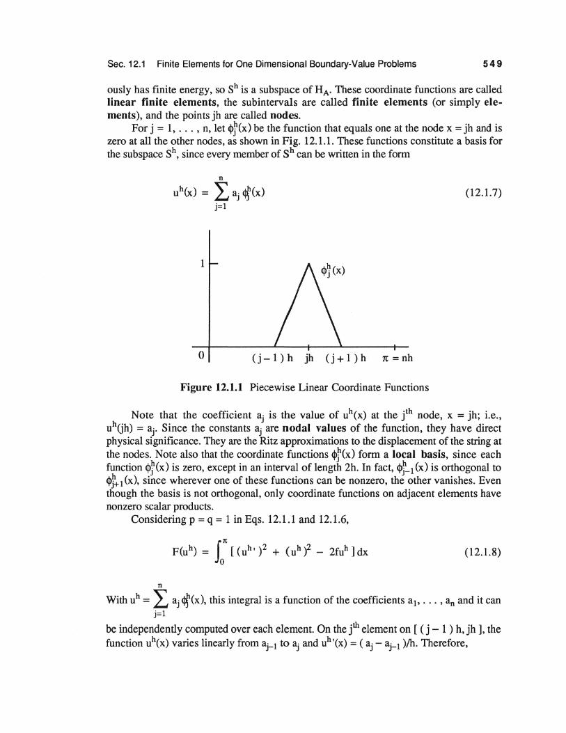
For j = 1, ... , n, let <!>f(x) be the function that equals one at the node x = jh and is zero at all the other nodes, as shown in Fig. 12.1.1. These functions constitute a basis for the subspace sh, since every member of sh can be written in the form

n

uh(x) = L aj qf(x) j=1

1

0 (j-1)h jh (j+1)h 1t=nh

Figure 12.1.1 Piecewise Linear Coordinate Functions

(12.1.7)

Note that the coefficient aj is the value of uh(x) at the j1h node, x = jh; i.e., uh(jh) = aj. Since the constants aj are nodal values of the function, they have direct physical significance. They are the Ritz approximations to the displacement of the string at the nodes. Note also that the coordinate functions <!>f(x) form a local basis, since each function <!>f(x) is zero, except in an interval of length 2h. In fact, <l>f-1 (x) is orthogonal to <Pf+ 1 (x), since wherever one of these functions can be nonzero, the other vanishes. Even though the basis is not orthogonal, only coordinate functions on adjacent elements have nonzero scalar products.

Considering p = q = 1 in Eqs. 12.1.1 and 12.1.6,

(12.1.8)

n

With uh = L aj <jf(x), this integral is a function of the coefficients a1, •.• , ~and it can j=l

be independently computed over each element. On the jth element on [ ( j - 1 ) h, jh ], the function uh(x) varies linearly from aj-1 to aj and uh'(x) = ( ajaj-1 )/h. Therefore,


Jjh (uh· )2 dx = ( aj - aj-1 r (j-1)h h

A similar computation yields

"h fj h ~ h ( 2 2 ) ( u J dx = -3 8.j + ajaj-1 + 8]-1

(j-1)h

For the entire interval [0, x], summing from Eqs. 12.1.9 and 12.1.10,

fo1t[(uh')2 + (uhf]dx

LN [ ( a· - a· 1 t - J J - h

j=1

(12.1.9)

(12.1.10)

(12.1.11)

It would be better to have this result as a quadratic form aTKa, since the positive semidefinite or positive definite global stiffness matrix K is needed. The expression F(uh) is quadratic in the vector parameter a= [ a1, ... , 8n ]T, of the form

F(uh) = aTKa - 2FTa (12.1.12)

The minimum of such an expression is thus determined by the matrix equation

Ka = F (12.1.13)

which is a necessary and sufficient condition for minimizing F(uh) ofEq. 12.1.12 if K is positive definite. Therefore, all that is needed is the matrix K and the vector F.

The contribution to K from each element; i.e., each subinterval of the string, can be found by returning to Eq. 12.1.9 and calculating the right side of the matrix form

"h fJ (uh' )2 dx (j-1)h

[ ] 1 [ 1 -1J[aj-1] = a· 1 a· -J- 1 h -1 1 a·

J

(12.1.14)

where k 1 is called an element stiffness matrix. Evaluation of k 1 needs to be done only once. Similarly, the calculation of the term in Eq. 12.1.10 over a single element is carried out only once, yielding the element mass matrix k0, defined by

"h [ ] J h 2 h 2 1 aj-1 f . ( u ) dx = [ aj-1 aj] 6 [ 1 2] . ~-1~ ~

(12.1.15)


The summation of Eqs. 12.1.14 and 12.1.15 over elements j = 1, ... , n defines the assembled global stiffness matrix K; i.e., the element matrices are added into proper positions in the global stiffness matrix.

The matrix associated with J ox ( uh' )2 dx, using the fact that ao = 0, is

1 0 1 -1 l 1 1

-1 1 0 1

0 0

Kl = h + + ... + h h 0 0 0 0 0 1 -1

-1 1

2 -1 0 0

1 -1 2 -1 0

= 0 -1 -1 0 (12.1.16) h

0 -1 2 -1 0 0 -1 1

The relationship between the matrix K1 and the integral of Eq.12.1.9 is

(12.1.17)

The integral of ( uh )2 is given by a TKoa, where the matrix Ko is formed by the same assembling process; i.e.,

4 1 0 0

h 1 4 1 0

Ko = 6 0 1 1 0 (12.1.18) 11 1 4 1 v

. 0 0 1 2

The Global stiffness matrix is thus obtained as K = K1 + Ko· Since the coefficients p(x) and q(x) in Eq. 12.1.6 depend on x, the integrals of

p(x) ( uh' )2 and q(x) ( uh )2 are computed numerically on each element. The assembled results are stored as stiffness matrices, whose quadratic forms are a TK1a and a TKoa.

It remains to compute the term

(12.1.19)

where


p. = rn fqf dx J Jo J

(12.1.20)

These tenns are computed by integrating over one element at a time. To summarize, writing K = K1 + Ko, the computations thus yield

(12.1.21)

This is the expression that is to be minimized in the Ritz method. The minimizing vector is thus determined by the matrix equation

Ka = F (12.1.22)

which is referred to as the finite element equation. If the element length h is small, Eq. 12.1.22 will be a large system of equations. If the operator A of Eq. 12.1.3 is positive definite, with boundary conditions accounted for, the matrix K is guaranteed to be positive definite and therefore invertable, since for p(x) > 0,

aTKa= Jn[p(x)(t ajqf'(x)J2

+ q(x)(t ajqf(x))2]dx ~ 0

0 J=l j=l (12.1.23)

n

can be zero only if L ajqf '(x) is identically zero and this happens only if aj = 0, j=l

j = 1, 2, ... , n. An extension of the foregoing development involves the introduction of finite ele

ments that are more refined than piecewise linear functions. A general function u(x) in C2(0, 1t) is better approximated by a higher degree polynomial. Therefore, it is natural to construct coordinate functions in spaces sh that are composed of polynomials of higher degree.

Quadratic Elements

As a first refinement, let sh consist of all piecewise quadratic functions that are continuous at the nodes x = jh and satisfy uh(O) = 0, called quadratic elements. The first objective is to determine the dimension of sh (the number of free parameters aj) and define a basis for sh. Note that continuity imposes only one constraint on the quadratic function at each node, so two coefficients in the polynomial remain arbitrary. Therefore, the dimension of sh is twice the number of quadratic functions, or 2n.

A basis for sh can be constructed by introducing the midpoints x = ( j - 1/2 ) h of the elements as nodes. There are then 2n nodes, since x = 0 is excluded and nh = 1t. Denote


them by zj, j = 1, ... , 2n. For each node, there is a continuous piecewise quadratic function that equals one at zj and zero at zi, for all i :t j; i.e.,

<l>i(zj) = oij (12.1.24)

These coordinate functions are of the three kinds shown in Fig. 12.1.2. Note that each is continuous and therefore in HA-

1

-.&...---+---'--x 0 h

Figure 12.1.2 Coordinate Functions for Piecewise Quadratic Elements

The quadratic approximate displacement on 0::::;; X::::;; h thus equals ao at X= 0, al/2 at the midpoint x = h/2, and a1 at x = h; i.e.,

u"(x) ; ao [ 1 - 3 G) + 2 ( ::) ] + ••12 [ 4 G) - 4 ( ::) ]

+a,[ -(~)+z(::)] (12.1.25)

The element stiffness matrix k tis computed by integrating ( uh '(x) )2 and writing the result as [ ao a112 a1 ] k1 [ ao a112 a1 ] • Notice that k1 is a 3 x 3 matrix, since only three of the parameters appear in any given interval. More specifically,

kl = -k -8 16 -8 [ 7 -8 1 ]

1 -8 7 (12.1.26)

Note that k 1 is singular, since applied to the nonzero vector [ 1, 1, 1 ]T, it yields the zero vector. This vector; i.e., ao = 1, a112 = 1, a1 = 1, corresponds to a quadratic function u(x) that is constant; i.e., u(x) = 1, so its derivative is zero. The matrix k0, in contrast, is nonsingular.

Cubic Elements

There is a cubic element that is better in almost every respect than the quadratic element just discussed. It is constructed by imposing continuity not only on the function u(x), but also on its first derivative. There is a double node at each point x = jh. Instead of being


determined by its values at four distinct points such as 0, h/3, 2h/3, and h, the cubic polynomial is now determined by its values and the values of its ftrst derivatives at two endpoints; i.e., by u0, Uo'· u1, and u1'. Both u1 and u1' are shared by the cubic in the next subinterval, thus assuring continuity of both u(x) and u'(x). These coordinate functions are shown in Fig. 12.1.3. These functions have a double zero at the ends (j ± 1 )h; i.e., the function and its ftrst derivative are both zero. They are called Hermite cubics.

IJI(O) = I ljlm

ro' (-1) = 0 co' (1) = 0

-h h

v( ~) = ( I ~ I - 1 f ( 21 ~ I + 1 )

Figure 12.1.3 Hermite Cubics

The cubic polynomial on 0 :S: x :S: h that takes on the values u0, u0', u1, and u1' is

(12.1.27)

The 4 x 4 element matrices are computed as follows, where a= [ Uo· Uo'· u1, u1' ]T:

mass matrix k0:

(12.1.28)


stiffness matrix k 1:

foh ( uh' )2 dx = aTkla (12.1.29)

bending matrix k2:

J oh ( u h " )2 dx = aT k2a (12.1.30)

Note that because uh(x) is in D2 n C1, it can be used in applications involving fourthorder operators, where the bending matrix k2 is needed.

One method of computing the ki is to form a matrix H that connects the four nodal parameters in the vector a to the four coefficients q = [ q0, q1, q2, 'b ]T of the cubic polynomial in Eq. 12.1.27 for uh(x) = ( q0 + q1x + q2x2 + q3x3 ); i.e., q = Ha. From Eq. 12.1.27,

1 0 0 0

rqo 0 1 0 0 uo

ql 3 2 3 1 uo' q = = h2 h h2 h = Ha (12.1.31) l qz ul

q3 2 1 2 1 ul' h3 h2 h3 h2

The integration of [ uh(x) ]2 in Eq. 12.1.28 yields

h h2 h3 h4

2 3 4

h2 h3 h4 h5 qo

J 0h ( u h i dx = [ qo ql q2 'b ]

2 3 4 5 ql = qTNoQ h3 h4 h5 h6 q2

3 4 5 6 q3

h4 h5 h6 h7

4 5 6 7 (12.1.32)

FromEqs.12.1.31 and 12.1.32,

h fo ( uh )2 dx = q TN0q = a THTN0Ha

so the element mass matrix is

k0 = HTN0H (12.1.33)


For the stiffness matrix, the only difference is that

0 0 0 0

0 h h2 h3

= qT 0 h2 4h3 3h4

q = qTNlq (12.1.34) T 2

0 h3 3h4 9h5

T T

so the element stiffness matrix is k1 = HTN1H.

ces: The results of these computations, and a similar one for k2, are the following matri·

156 22h 54 -13h

h 22h 4h2

ko = 420 54 13h 13h -3h2

156 -22h

-13h -3h2 -22h 4h2

36 3h -36 3h

1 3h 4h2 -3h -h2

kl = 30h -36 -3h 36 -3h

3h -h2 -3h 4h2

12 6h -12 6h

1 6h 4h2 -6h 2h2

k2=h3 -12-6h 12 -6h

6h 2h2 -6h 4h2

(12.1.35)

(12.1.36)

(12.1.37)

The matrix ko is ~ositive definite, but k 1 has a zero eigenvalue that corresponds to the constant function u (x) = 1; i.e., to a= [ 1, 0, 1, 0 ]r. The matrix k2 is also singular, since for every linear uh(x), uh "(x) = 0.

A fourth order beam equation

Au = ( ru" )" - ( pu' )' + qu = f (12.1.38)

with r(x) ~ rmin > 0, p(x) ~ 0 and q(x) ~ 0 can now be treated. With physically reasonable boundary conditions, the associated energy scalar product is


[ u, v ]A = Ion: ( ru"v" + pu'v' + quv ) dx (12.1.39)

and the Minimum Functional Theorem leads to F(u) = [ u, u ]A- 2 ( f, u ). For the Ritz method to apply, the coordinate functions must have finite energy, which means they must be in D2 n C1. The Hermite cubics are therefore applicable.

If a beam is clamped at x = 0, the boundary conditions at x = 0 are

u(O) = u'(O) = 0 (12.1.40)

which are principal. The candidate solution u\x) must have a double zero at x = 0; i.e., it must satisfy Eq. 12.1.40. To see what the natural boundary conditions are at x = rc, integrate F(u) by parts and require that its first variation vanishes. The result is that, for every ou in the admissible space D2 n C1,

oF :::: s: [ (ru" )" - (pu' )' + qu- f] Ou dx + ru"ou' I: + (pu'- (ru")')oul: = 0 (12.1.41)

Thus, the natural boundary conditions on u(x) are those that physically correspond to a free end; i.e.,

u" (rc) = 0

[ pu' - (ru" )' ](rc) = 0 (12.1.42)

These are the well known zero moment and zero shear conditions at the free end of a beam [25].

Finite elements with Hermite cubic coordinate functions of Eq. 12.1.27 may be selected, which satisfy boundary conditions of Eq. 12.1.40, but not Eq. 12.1.42. Presuming r(x), p(x), and q(x) are piecewise constant on the elements, the element matrices of Eqs. 12.1.35 through 12.1.37 may be applied in Eqs. 12.1.28 through 12.1.30. Thus,

n

= I, [ aiTrJ,2ai + aiTPiklai + aiTqikoai - 2aiTFi] i=l

and the Ritz equations are

Ka = F

(12.1.43)

(12.1.44)


12.2 FINITE ELEMENTS FOR TWO DIMENSIONAL BOUNDARY-VALUE PROBLEMS

While development of the fmite element method for elliptic partial differential equations in two independent variables is theoretically no more difficult than for problems with only one independent variable, the algebraic complexity is somewhat greater. For this reason, attention is restricted to a general description of the method and the reader is referred to the literature for detailed development of element formulas [25, 27]. In this section, some finite elements in the plane are defined. Development of such elements involves only elementary algebra, but the results are of great importance. The goal is to choose piecewise polynomials that are determined by a small set of nodal values, and yet have the desired degree of continuity.

There are many triangular and rectangular finite elements, and it is not clear whether it is more efficient to subdivide the region into triangles or rectangles. Triangles are better for approximating a curved boundary, but there are advantages to rectangles in the interior. There are fewer of them, and they permit very simple elements of high degree.

Consider first subdividing the region Q into triangles, as shown in Fig. 12.2.1. The union of these triangles is a polygon nh. The longest edge of the ith triangle will be denoted by hi and h =max hi. Assume that no vertex zj = Cx{, x~) of one triangle lies on the edge of another triangle.

Figure 12.2.1 Subdivision of the Region n into Triangular Elements

Linear Triangular Elements

Given a triangulation, the simplest of all coordinate functions is the linear coordinate function uh(x1, x2) = a1 + a2x1 + a3x:y; inside each triangle, which must be continuous across each edge. Thus, the graph of u (x1, x2) is a surface that is made up of plane triangular pieces, joined along their edges. This is a generalization of the piecewise linear functions in one dimension used in Section 12.1. The space Sh of these piecewise linear functions is a subspace of D1(Qh) n c0(Qh), whose first derivatives are piecewise constant. As seen in Chapter 9, this class of functions is reasonable for solution of second order equations. It is not regular enough, however, for fourth order equations.

Sec. 12.2 Finite Elements for Two Dimensional Boundary-Value Problems 559

The simplicity of piecewise linear functions lies in the fact that within each triangle, the three coefficients of uh(x1, x2) = a1 + a2x1 + a3x2 are uniquely determined by the nodal values of uh(x1, x2) at the three vertices. Furthermore, along any edge uh(x1, x2) reduces to a linear function of the arc length variable along that edge and this function is detennined by its values at the two endpoints of the edge. The value of uh(x1, x2) at the third vertex has no effect on the function along this edge. Therefore, continuity of uh(x1, x2) across the edge is assured by continuity at the vertices.

For a principal boundary condition, say u(x1, x2) = 0 on r, the simplest space sh is formed by requiring the functions to be zero on the polygonal boundary 'fh shown in Fig. 12.2.1. The dimension of the space Sh; i.e., the number n of free parameters in the functions uh(x1, x2), is the number of unconstrained nodes. Let (j)j(x1, x2) be a coordinate function that equals 1 at the jth node and zero at all other nodes, as shown in Fig. 12.2.2. These pyramid functions (j)j(x 1, x2) form a basis for the space sh. An arbitrary uh(x1, x2) in sh can be expressed as

n

uh(xl, x2) = L aj ~(xl, x2) j=l

(12.2.1)

~e nodal coo.rdi~ate aj has the physical significance of displacement uh(x1, x2) at the J node zj = (x{, x~).

Figure 12.2.2 Pyramid Coordinate Function

The coordinates aj are determined by minimizing the energy functional F(uh), which n

is quadratic in a1, ..• , ~·The minimizing function uh(x 1, x2) = L aj ~(x 1 , x2) is dej=l


tennined by the solution of a matrix equation of the form

Ka = F

The matrix K is well conditioned and sparse, since two nodal coordinates are coupled only if they belong to the same element. Furthermore, the coefficients ~j = [ <Pi• <l>j ]A and Fj = ( f, <l>j ) in the Ritz equation can be found by a systematic evaluation of scalar products from the triangular elements, one at a time. This means that the integrals are computed over each element, yielding a set of element stiffness matrices ki, involving only the nodes of the ith triangle of the finite element grid. The global stiffness matrix K that contains all such scalar products is then assembled from these pieces. This process is carried out just as in the one dimensional case developed in Section 12.1.

Quadratic Triangular Elements

Consider next a more refined element. Rather than using a linear function within each triangle, uh(x1, x2) will be the quadratic coordinate function

(12.2.2)

In order to be in D1 n C0, uh(x1, x2) must be continuous across edges between adjacent triangles. To define a basis for this space, a set of continuous piecewise quadratic functions <!>ix1, x2) must be found, such that every member of sh has a unique expansion as

n

uh(xl' x2) = L aj ~(xl' xz) j=l

(12.2.3)

To form such a basis, additional nodes may be placed at the midpoints of the edges, as in Fig. 12.2.3(a). With each node, whether it is a vertex or the midpoint of an edge, the coordinate function <!>j(x 1, x2) is defined as 1 at that node and zero at all others. This rule specifies <l>j(x1, x2) at six points in each triangle, the three vertices and three midpoints, thereby determining the six coefficients in Eq. 12.2.2.

The piecewise quadratic coordinate function that is determined by this rule, in each separate triangle, must be shown to be continuous across edges between triangles. Along an edge, uh(x1, x2) is quadratic in the boundary arc length variable and there are three nodes on the edge. Therefore, the quadratic polynomial is uniquely detennined by the three nodal values that are shared by the triangles that meet at that edge. The nodal values elsewhere in the triangles have no effect on uh(x1, x2) along the edge, so continuity holds. For an edge that is on the outer boundary rh with boundary condition u = 0, the quadratic is zero.

n

Any uh(x 1, x2) in sh can be expressed as uh(x 1, x2) = L aj ~(x 1 , x2), where the j=l

nodal coordinate aj is the value of u\x1, x2) at the jth node. Therefore, these <!>j(x 1, x2)

form a basis for sh and its dimension is the number of unconstrained nodes.


(b) D1 cubic (a) D1 quadratic

-1 (c) D cubic

Figure 12.2.3 Nodal Placement for Quadratic and Cubic Elements

Cubic Triangular Elements

Using continuous piecewise cubic polynomials, a basis can be constructed in a similar way. A cubic in the variables x1 and x2 is determined by 10 coefficients, in particular by its values at the 10-node triangle of Fig. 12.2.3(b ). The 4 nodes on each edge determine the piecewise cubic coordinate function uniquely on that edge, so continuity is assured.

In the cubic case of Fig. 12.2.3(c), the condition that the first derivatives of uh(x1, x2) should be continuous at every vertex can be added. This is clearly a subspace of the previous cubic case, in which only continuity of uh(x1, x2) was required. If m triangles meet at a given interior vertex, the continuity of u~ (x 1, x2) and u~. (x 1, x2) imposes new constraints on the coordinate functions, so the dimeAsion is correspJndingly reduced. To construct a basis for sh, the midedge nodes are removed and a triple node is defined at each vertex, as shown in Fig. 12.2.3(c). The 10 coefficients in the cubic are determined by u, ux , and ux at each vertex, together with u at the centroid. A unique cubic is determined by these fO nodal values. Along each edge, it is determined by a subset of four of the values of u(x) and its first derivative along the edge at each end, a combination that assures matching along the edge. The result is a useful set of cubic coordinate functions in D1(Qh), denoted D1.

Piecewise polynomial finite elements in D1 are easy to describe in the interior of the domain, but care is required at the boundary. In the case of a principal boundary condition U(Xl, Xz) :::: 0 On f, there is first the COnstraint Uh(xl, Xz) ::::: 0 along all Of fh. Thus, the derivatives along both element boundary edges must be set equal to zero, leaving no parameters free at that vertex.


Quintic Triangular Elements

None of the spaces defined above can be applied to the biharmonic equation, since they are not subspaces of D2 n C1. In order to construct coordinate functions that belong to C1,

the normal derivative must be continuous across element boundaries. If piecewise polynomials are to be used, they must be of fifth degree; i.e., quintics.

A polynomial of fifth degree in x1 and x2 has 21 coefficients to be determined, of which 18 can come from the values of u, Ux , ux , Ux x , ux x , and Ux x at the vertices. Th d d . . b d" 1 2 1 1 h 1 2 f f' 2 • al . . ese secon envatlves represent en mg moments t at are o pnys1c Interest m plates; e.g., Eq. 11.4.11, which will be continuous at the vertices and available as output from the finite element analysis process. Furthermore, with all second derivatives present, there is no difficulty in allowing an irregular finite element triangulation. The piecewise quintic coordinate function along the edge between two triangles is the same from both sides, since conditions are shared at each end of the edge on u and its first two tangential derivatives us and uss• which are computable from the set of six parameters at each vertex.

It remains to determine three more constraints in such a way that the normal derivative un(x1, x2) is also continuous across edges. One technique is to add the value of tin at the midpoint of each edge to the first of nodal parameters, as shown in Fig. 12.2.4(a). Then, since un(x1, x2) is a fourth degree polynomial ins along the edge, it is uniquely determined by this midpoint nodal value of tin and the values of lin and Uns at each end. The normal n at the middle of an edge points into one triangle and out of the adjacent one, somewhat complicating the bookkeeping. This construction produces a complete C1 n D2

quintic.

(u, ... ) (u, ... )

(a) Full Fifth Degree Element (b) Reduced Fifth Degree Element

Figure 12.2.4 Two Fifth Degree Triangles

Another way of determining the three remaining constraints is to require that un(x1, x2) reduces to a cubic along each edge; i.e., that the leading coefficient in what would otherwise be a fourth degree polynomial vanishes. With this constraint, the nodal


values of Un and 11ns determine the cubic Un(x1, x2) along the edge, and the element is in C1 tl D2. The complete quintic is lost, however, reducing the order of displacement error [27]. At the same time, the dimension of sh is significantly reduced (see Fig. 12.2.4(b)).

Rectangular Elements

Consider next rectangular elements. A number of important problems in the plane are defined on a rectangle or on a union of rectangles. The boundary of a more general region cannot be described sufficiently well without using triangles, but it will often be possible to combine rectangular elements in the interior, with triangular elements near the boundary.

The simplest coordinate functions on rectangles are piecewise bilinear functions; i.e., uh(x1, x~) = c1 + c2x1 + c3x2 + c4x1x2• The four coefficients are determined by the values of u at the vertices. There is thus a set of piecewise bilinear coordinate functions, in which <l>j(x1, x2) is 1 at node j and is 0 at the others. It is a product 'lf(x1) v(x2) of piecewise linear functions in one variable, so that the space sh is a product of two simpler spaces. Such elements are called bilinear rectangular elements. They are continuous, so they can be used for second order problems. Bilinear elements on rectangles can be merged with linear elements on triangles, since both are completely determined by the value of uh at the nodes.

One other rectangular element is defined here, as an extension of the one-dimensional Hermite cubic element of Fig. 12.1.3. The basis in one dimension contains two kinds of functions, 'If( X) and ro(x), which interpolate values of the function and its first derivative, respectively,

{ 1, at node x = xj

'Vj = 0, at other nodes

d'tf. dxJ = 0, at all nodes,

roj = 0, at all nodes

dmj = { 1, at node x = xj

dx 0, at other nodes

The Hermite bicubic space is a product of two such cubic spaces. The four parameters at a typical node Cx{, x~) lead to four corresponding coordinate functions,

<1>1 (x1, x2) = 'Vi(xl) 'l'j(x2), <!2(xl, x2) = 'Vi(xl) ro/x2)

<I>J(xl, x2) = Ol_j(xl) v/x2), <!>4(xl, x2) = Ol_j(xl) ro/x2) (12.2.4)

The degree of continuity of the Hermite bicubic coordinate functions follows immediately from the basis given in Eq. 12.2.4. Since 'lf(Xl) and co(x2) are both in C1' all their products have this property. Therefore, this bicubic may be applied to fourth-order equations. The trial functions lie in D2. Furthermore, even the cross derivatives Ux x (xl, x2) are continuous.

1 2 The rather messy algebra and calculus that must be carried out to form the Ritz equations,


(12.2.5)

for the operator equation Au = f are not developed here. The reader who wishes to go into such detail is referred to the extensive finite element literature [25, 27, 28].

12.3 FINITE ELEMENT SOLUTION OF A SYSTEM OF SECOND ORDER PARTIAL DIFFERENTIAL EQUATIONS

Second Order Plate Boundary-Value Problems

The governing equations for bending of a plate can be written, as in Eq. 11.4.11, as

Az =

12 12v ()2z4 - Eh3 Zt + Eh3 ~ - axr

12v 12 o2z4 Eh3 Zt - Eh3 z2 - axi

24 (1 + v ) ()2z4 Eh3 z3 + 2 dxt dx2

a2zl a2z2 a2z3

- axr - axi + 2 ax 1 dx2

= [~] (12.3.1)

where z1 (x1, x2) and z2(x1, x2) are bending moments on cross sections normal to the x1

and x2 axes, respectively, z3(x1, x2) is the torsional moment on a cross section normal to either the x1 or x2 axes, z4(x1, x2) is displacement in the direction normal to the plate middle surface, vis Poisson's ratio, his the thickness of the plate, and f(x1, x2) represents the distributed load.

For the rectangular plate of Fig. 12.3.1 that is simply supported along its edges, the boundary conditions are

(12.3.2)

On the other hand, if the plate is clamped along its edges, the boundary conditions are

dZ4 dZ4 -=r- (±a, x2) = -s- (x1, ±b)= z4(± a, x2) = z4(xl> ±b)= 0 (12.3.3) ox1 ux2

It may be noted that having the slope equal to zero along the boundary implies that z3(x1, x2) is equal to zero along the boundary. The latter condition can be handled more easily and will be used to solve clamped plate problems.

Sec. 12.3 Finite Element Solution of a System of Second Order Partial Differential Eqns. 56 5

-a (A)

-b

a (B)

""' X 1

Figure 12.3.1 Rectangular Plate

Galerkin Approximate Solution

Here, the plate problem is solved by the finite element Galerkin method, for comparison with numerical results of Section 11.4. A stiffness matrix is formulated for the system of partial differential equations of Eq. 12.3.1. To formulate the finite element approximation, an element geometry must first be chosen. Considering the rectangular shape of the plate in Fig. 12.3.1, a rectangular element is chosen, with the eight nodes shown in Fig. 12.3.2. The equations contain four unknown variables zi(x1, x2), i = 1, ... , 4, which can be approximated by their values, Zf, i = 1, ... , 4, a = 1, ... , 8, at the nodes; i.e.,

8

zNx1, x2) = L :qa <l>a(x1, x2), i = 1, ... , 4 a=l

8

tf(xl, x2) = L Ff<l>a(xl, x2), i = 1, ... , 4 a=l

(12.3.4)

where the <l>a(x1, x2) are coordinate functions. Note that for computational convenience, the forcing functions fi(x1, x2) have been expanded in terms of the coordinate functions. A higher order element that is developed in Ref. 28 is used. Details of the calculations are not presented here.

3 2 1

4 8

5 6 7

Figure 12.3.2 Element with Eight Nodes


Using the Galerkin techni~ue, the differential equations may be reduced to a stiffness matrix and force vector on the i element, given symbolically by

12 - Eh3 clla<P~

12v Eh3 <Pa<P~

12v 12 8 Eh3 <Pa<P~ - Eh3 <Pacll~

JJn I 1 a.= I

0 0

a2c~>« a2<Pa --cp~ --cp~

ax2 a xi 1

0 a2clla

--cp~ axr

a2c~>a z~ 0 --<1>13

~ axi

_24(1+v)cpcp 2 a2<Pa cp ~ Eh3 a 13 axl ax2 ~ za

a2c~> 2 a cp

axl ax2 13

Ff<Pa<P~

~<Pa<Pp

F~<Pa<Pp

f1<Pa<P13 i

4

0

dxt dx2 = 0, ~ = 1, ... , 8

By performing integration by parts, the above relation yields

12 12v 0

o<Pa acp13 - Eh3 <Pacl>p Eh3 cp11cl>p --axl axl

12v 12 acpa ac~>~ z~ 8 Eh3 <Pa<Pp - Eh3 <Pa<P~ 0

ax2 ax2 ~ If~ I a.= I

0 0 _24(1+v)cjlcp ac~>a acp~ ac~>a acp13 ~ Eh3 ~~ 13 - axl ax2 - ax2 axl z~~

4

dcjla dcpp o<Pa acp13 o'Pa acp13 o<Pa o<Pp 0

axl OXt ax2 ax2 - axl ax2 - ax2 axl

F~<Pa<Pp

F~cjl~~cl>p

F~<Pacl>p

F~cllacllp i

dx1 dx2 = 0, ~ = 1, ... , 8 (12.3.5)

where oi is the subdomain corresponding to the ith element. After integration, Eq. 12.3.5 becomes

k·Z· = F· 1 1 1 (12.3.6)

where ki is a stiffness matrix for the ith element. This integration over a subdomain may

Sec. 12.3 Finite Element Solution of a System of Second Order Partial Differential Eqns. 56 7

be conveniently carried out by introducing local coordinates and using a Gaussian quadrature formula. The details are explained in Ref. 28. Assembling Eq. 12.3.6 for each element yields a system of linear equations

Kz = F (12.3.7)

that represents the finite element approximation of the system of plate equations of Eq. 12.3.1.

In order to compare with numerical results of Section 11.4, the following square plate problems are analyzed:

(1) simply supported boundary (2) clamped boundary

For each boundary condition, the following thicknesses are studied:

( 1) uniform thickness

(2) varying thickness h(x 1, x2) = 2 ( 1- I : 1 I ) ( 1- I : 21 ) ho

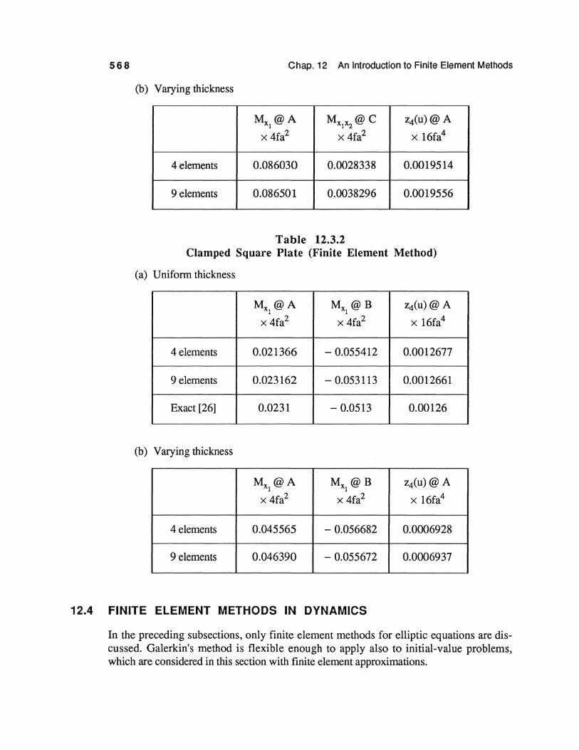
Numerical results for four test problems are presented in Tables 12.3.1 and 12.3.2. Note that the finite element method gives consistently good approximations, in comparison with results presented in Section 11.4.

Table 12.3.1 Simply Supported Square Plate (Finite Element Method)

(a) Uniform thickness

4elements

9 elements

Exact [26]

ax2 a

c

Mx @A 1

x 4fa2

0.048206

0.047855

0.0479

Mxx @C 1 2

z4(u)@ A

x 4fa2 x 16fa4

0.034505 0.0040563

0.033768 0.0040612

0.0325 0.00406


(b) Varying thickness

Mx @A 1

Mxx @C 1 2

z4(u)@ A

x 4fa2 x 4fa2 x 16fa4

4elements 0.086030 0.0028338 0.0019514

9 elements 0.086501 0.0038296 0.0019556

Table 12.3.2 Clamped Square Plate (Finite Element Method)

(a) Uniform thickness

Mx @A I

Mx @B 1

z4(u)@ A

x 4fa2 x 4fa2 x 16fa4

4 elements 0.021366 - 0.055412 0.0012677

9 elements 0.023162 -0.053113 0.0012661

Exact [26] 0.0231 -0.0513 0.00126

(b) Varying thickness

Mx @A 1

Mx @B l

z4(u)@ A

x4fa2 x 4fa2 x 16fa4

4 elements 0.045565 -0.056682 0.0006928

9 elements 0.046390 -0.055672 0.0006937

12.4 FINITE ELEMENT METHODS IN DYNAMICS

In the preceding subsections, only finite element methods for elliptic equations are discussed. Galerkin's method is flexible enough to apply also to initial-value problems, which are considered in this section with finite element approximations.

Sec. 12.4 Finite Element Methods in Dynamics 569

The Heat Equation

A natural setting in which to illustrate the finite element method for dynamics is the heat equation,

h(x, t), 0 < x < 1t, t > 0 (12.4.1)

This parabolic differential equation represents heat conduction in a rod, where u(x, t) is the temperature at point x and timet> 0 and h(x, t) is a heat-source term. Boundary conditions at x = 0 and at x = 1t are

au u(O, t) = ax (1t, t) = 0, t>O (12.4.2)

The first condition means physically that the temperature at the left end of the rod is held at 0. The second condition means that the right end of the rod is insulated, so there is no temperature gradient at x = 1t. To complete the statement of the problem, the initial temperature is

u(x, 0) = f(x), 0 $ x S 1t (12.4.3)

This classical formulation of heat conduction is fraught with difficulties. For example, Eqs. 12.4.2 and 12.4.3 are contradictory if f(x) fails to vanish at x = 0, or if iJf(x)/iJx does not vanish at x = 1t. In addition, h(x, t) could be a point source at x0, which is singular, so Eq. 12.4.1 is not meaningful at that point. In each of these cases, the underlying physical problem still makes sense.

Since the equation is not symmetric, the Galerkin formulation is employed. At each time t > 0, it is desired that for arbitrary v(x) in C2(0, 1t),

f 01t ( Ut - Uxx - h ) v dx = 0 (12.4.4)

In the steady state, with ut(x, t) = 0 and h(x, t) = h(x), this coincides with the earlier Galerkin formulation.

To achieve some symmetry, integrate the term- uxxv in Eq. 12.4.4 by parts. The boundary term ux v vanishes at x = 1t and it is required that v(O) = 0. Equation 12.4.4 then becomes

(12.4.5)

for all v(x) in HA (0, 1t).

This is the starting point for finite element approximation. Given ann-dimensional subspace sh of HA (0, 7t), the goal of the Galerkin method is to find a function uh(x, t)


that, for each t > 0, is in sh of Section 12.1 and satisfies

(12.4.6)

for all vh(x) in sh. Notice that the time variable is still continuous; i.e., the Galerkin formulation is dis

crete in the space variables and yields a system of ordinary differential equations in time. It is these equations that must be solved numerically. To make this formulation useful, a basis { cl>i(x) } is chosen for the space sh and the unknown solution is expanded as

n

uh(x, t) = I, q/t) <!>/x) j=l

The coefficients qj(t) are determined by the Galerkin method; i.e.,

n f1t[. a~ a<lk J ~ 0 qj<J>j<l>k + qj ax ax - h<J\c dx = 0, k = 1, ... , n j=l

(12.4.7)

(12.4.8)

Since every vh(x) is a combination of the coordinate functions <l>k.(x), it is enough to apply the principle only to these functions. The result is a system of n ordinary differential equations for the n unknowns, q1 (t), ... , ~(t), and the initial condition u(x, 0) = f(x) is still to be accounted for. Equation 12.4.8 may be rewritten as

t, [ <i/t) I: <I\ <Ilk dx + qj ( <1\' <l>k dx ] = r h(x, t) <l>k(x) dx,

k = 1, ... , n (12.4.9)

Defining

m 'k = f1t <!>·<l>k dx J Jo J

kij = 11t <!>j '<l>k' dx (12.4.10)

Pk(t) = fo1t h(x, t) <l>k dx

Eqs. 12.4.9 may be written in matrix form as

Mq + Kq = p(t) (12.4.11)

Sec. 12.4 Finite Element Methods in Dynamics 571

where M and K are n x n symmetric, positive definite matrices. This system of equations can be solved numerically by efficient numerical integration techniques for q(t) = [ q1 (t), ... , 'fu(t) ]T. The result may be substituted into Eq. 12.4.7, to obtain the approximate solution of the transient heat problem.

Hyperbolic Equations

As an introduction to the finite element method for hyperbolic equations, consider the dynamics problem

Uu + Au = h(x, t)

u(x, 0) = f(x), ut(x, 0) = g(x) (12.4.12)

with x in Q c Rn and u(x, t) in D A• which is a subset of c2m(Q x T) that satisfies homogeneous boundary conditions, A is a positive definite operator of order 2m for fixed t, and h(x, t) is the forcing function.

The Galerkin method begins by requiring that, for all v(x) in D A and for all t,

( Uu, v ) + ( Au, v ) = ( h, v ) (12.4.13)

Integrating by parts in the second term on the left,

( Uu, V ) + [ U, V ]A = ( h, V ) (12.4.14)

for all v(x) in HA and t > 0. In the Galerkin approximation, u(x, t) and v(x) are replaced n

by uh(x, t) = L q/t) $j(x) and vh(x) in sh. The time dependent coefficients qj(t), j=l

j = 1, ... , n, are determined by

n n

L qj ( $j, 4\) + L qj [ $j, <1>k ]A= ( h, <1\c ), k = 1, ... , n (12.4.15) j;l j=l

This is an ordinary differential equation in the time variable. In this case, the same mass and stiffness matrices as in the parabolic case appear, but the equation is of second order; i.e.,

Mq + Kq = p(t) (12.4.16)

Since the matrices M and Kin Eq. 12.4.16 are positive definite, methods of matrix differential equations may be directly applied. The equations may be decoupled using a modal matrix transformation and the resulting simple second order scalar differential equations may be solved in closed form, or with simple and effective numerical integration methods. This method is routinely applied in the field of structural mechanics, with good results.

AN INTRODUCTION TO FINITE ELEMENT METHODSuser.engineering.uiowa.edu/~kkchoi/Chapter_12.pdf552 Chap....

Documents

Transcript of AN INTRODUCTION TO FINITE ELEMENT METHODSuser.engineering.uiowa.edu/~kkchoi/Chapter_12.pdf552 Chap....