Finite Difference, Finite Element and Finite Volume...
148
Finite Difference, Finite Element and Finite Volume Methods for the Numerical Solution of PDEs Vrushali A. Bokil [email protected] and Nathan L. Gibson [email protected] Department of Mathematics Oregon State University Corvallis, OR DOE Multiscale Summer School June 30, 2007 Multiscale Summer School – p. 1
Transcript of Finite Difference, Finite Element and Finite Volume...

Finite Difference, Finite Element and Finite
Volume Methods for the Numerical Solution of
PDEsVrushali A. Bokil
and
Nathan L. [email protected]
Department of Mathematics
Oregon State University
Corvallis, OR
DOE Multiscale Summer SchoolJune 30, 2007
Multiscale Summer School – p. 1

Math Modeling and Simulation of Physical Processes
• Define the physical problem
• Create a mathematical (PDE) model• Systems of PDEs, ODEs, algebraic equations• Define Initial and or boundary conditions to get a
well-posed problem
• Create a Discrete (Numerical) Model• Discretize the domain → generate the grid → obtain
discrete model• Solve the discrete system
• Analyse Errors in the discrete system• Consistency, stability and convergence analysis
Multiscale Summer School – p. 2

Math Modeling and Simulation of Physical Processes
• Define the physical problem
• Create a mathematical (PDE) model• Systems of PDEs, ODEs, algebraic equations• Define Initial and or boundary conditions to get a
well-posed problem• Create a Discrete (Numerical) Model
• Discretize the domain → generate the grid → obtaindiscrete model
• Solve the discrete system
• Analyse Errors in the discrete system• Consistency, stability and convergence analysis
Multiscale Summer School – p. 2

Math Modeling and Simulation of Physical Processes
• Define the physical problem
• Create a mathematical (PDE) model• Systems of PDEs, ODEs, algebraic equations• Define Initial and or boundary conditions to get a
well-posed problem• Create a Discrete (Numerical) Model
• Discretize the domain → generate the grid → obtaindiscrete model
• Solve the discrete system• Analyse Errors in the discrete system
• Consistency, stability and convergence analysis
Multiscale Summer School – p. 2

Contents• Partial Differential Equations (PDEs)
• Conservation Laws: Integral and DifferentialForms
• Classification of PDEs: Elliptic, parabolic andHyperbolic
• Finite difference methods• Analysis of Numerical Schemes: Consistency,
Stability, Convergence• Finite Volume and Finite element methods• Iterative Methods for large sparse linear systems
Multiscale Summer School – p. 3

Contents• Partial Differential Equations (PDEs)• Conservation Laws: Integral and Differential
Forms
• Classification of PDEs: Elliptic, parabolic andHyperbolic
• Finite difference methods• Analysis of Numerical Schemes: Consistency,
Stability, Convergence• Finite Volume and Finite element methods• Iterative Methods for large sparse linear systems
Multiscale Summer School – p. 3

Contents• Partial Differential Equations (PDEs)• Conservation Laws: Integral and Differential
Forms• Classification of PDEs: Elliptic, parabolic and
Hyperbolic
• Finite difference methods• Analysis of Numerical Schemes: Consistency,
Stability, Convergence• Finite Volume and Finite element methods• Iterative Methods for large sparse linear systems
Multiscale Summer School – p. 3

Contents• Partial Differential Equations (PDEs)• Conservation Laws: Integral and Differential
Forms• Classification of PDEs: Elliptic, parabolic and
Hyperbolic• Finite difference methods
• Analysis of Numerical Schemes: Consistency,Stability, Convergence
• Finite Volume and Finite element methods• Iterative Methods for large sparse linear systems
Multiscale Summer School – p. 3

Contents• Partial Differential Equations (PDEs)• Conservation Laws: Integral and Differential
Forms• Classification of PDEs: Elliptic, parabolic and
Hyperbolic• Finite difference methods• Analysis of Numerical Schemes: Consistency,
Stability, Convergence
• Finite Volume and Finite element methods• Iterative Methods for large sparse linear systems
Multiscale Summer School – p. 3

Contents• Partial Differential Equations (PDEs)• Conservation Laws: Integral and Differential
Forms• Classification of PDEs: Elliptic, parabolic and
Hyperbolic• Finite difference methods• Analysis of Numerical Schemes: Consistency,
Stability, Convergence• Finite Volume and Finite element methods
• Iterative Methods for large sparse linear systems
Multiscale Summer School – p. 3

Contents• Partial Differential Equations (PDEs)• Conservation Laws: Integral and Differential
Forms• Classification of PDEs: Elliptic, parabolic and
Hyperbolic• Finite difference methods• Analysis of Numerical Schemes: Consistency,
Stability, Convergence• Finite Volume and Finite element methods• Iterative Methods for large sparse linear systems
Multiscale Summer School – p. 3

Partial Differential Equations• PDEs are mathematical models of continuous physical
phenomenon in which a dependent variable, say u, is afunction of more than one independent variable, say t (time),and x (eg. spatial position).
• PDEs derived by applying a physical principle such asconservation of mass, momentum or energy. Theseequations, governing the kinematic and mechanicalbehaviour of general bodies are referred to as ConservationLaws. These laws can be written in either the strong ofdifferential form or an integral form.
• Boundary conditions, i.e., conditions on the (finite)boundary of the domain ann/or initial conditions (fortransient problems) are required to obtain a well posedproblem.
Multiscale Summer School – p. 4
PDEs (continued)• For simplicity, we will deal only with single
PDEs (as opposed to systems of several PDEs)with only two independent variables,• either two space variables, denoted by x and
y, or• one space variable denoted by x and one time
variable denoted by t
• Partial derivatives with respect to independentvariables are denoted by subscripts, for example• ut = ∂u
∂t
• uxy = ∂2u∂x∂y
Multiscale Summer School – p. 5

Well Posed Problems• Boundary conditions, i.e., conditions on the
(finite) boundary of the domain and/or initialconditions (for transient problems) are required toobtain a well posed problem.
• Properties of a well posed problem:• Solution exists• Solution is unique• Solution depends continuously on the data
Multiscale Summer School – p. 6

Classifications of PDEs• The Order of a PDE = the highest-order partial
derivative appearing in it. For example,• The advection equation ut + ux = 0 is a first
order PDE.• The Heat equation ut = uxx is a second order
PDE.
• A PDE is linear if the coefficients of the partialderivates are not functions of u, for example• The advection equation ut + ux = 0 is a linear
PDE.• The Burgers equation ut + uux = 0 is a
nonlinear PDE.
Multiscale Summer School – p. 7

Classifications of PDEs• The Order of a PDE = the highest-order partial
derivative appearing in it. For example,• The advection equation ut + ux = 0 is a first
order PDE.• The Heat equation ut = uxx is a second order
PDE.• A PDE is linear if the coefficients of the partial
derivates are not functions of u, for example• The advection equation ut + ux = 0 is a linear
PDE.• The Burgers equation ut + uux = 0 is a
nonlinear PDE.
Multiscale Summer School – p. 7

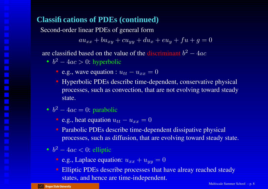
Classifications of PDEs (continued)Second-order linear PDEs of general form
auxx + buxy + cuyy + dux + euy + fu + g = 0
are classified based on the value of the discriminant b2 − 4ac• b2 − 4ac > 0: hyperbolic
• e.g., wave equation : utt − uxx = 0
• Hyperbolic PDEs describe time-dependent, conservative physicalprocesses, such as convection, that are not evolving toward steadystate.
• b2 − 4ac = 0: parabolic• e.g., heat equation utt − uxx = 0
• Parabolic PDEs describe time-dependent dissipative physicalprocesses, such as diffusion, that are evolving toward steady state.
• b2 − 4ac < 0: elliptic• e.g., Laplace equation: uxx + uyy = 0
• Elliptic PDEs describe processes that have alreay reached steadystates, and hence are time-independent.
Multiscale Summer School – p. 8

Parabolic PDEs: Initial-Boundary value problems
• Example: One dimensional (in space) Heat Equation for u = u(t, x)
ut = κuxx, 0 ≤ x ≤ L, t ≥ 0
• with• Boundary conditions: u(t, 0) = u0, u(t, L) = uL, and• Initial conditions: u(0, x) = g(x)
t
tp
0 xxp L
p
domain of dependence
domain of influence
0
Multiscale Summer School – p. 9

Elliptic PDEs: Boundary value problems
• Example: Model of steady heat conduction in a two dimensional (inspace) domain, governed by the Laplace equation for the temperatureT = T (x, y)
Txx + Tyy = 0, 0 ≤ x ≤ W, 0 ≤ y ≤ H
• with boundary conditions• T (x, 0) = T1, T (x, H) = T3
• T (0, y) = T4, T (W, y) = T2
y
yp
0 xxp W
p
0
H
T1
T2
T3
T4
Multiscale Summer School – p. 10

Hyperbolic PDEs: Initial-Boundary value problems
• Example: One-dimensional (in space) wave equation for u = u(t, x)
utt = c2uxx, 0 ≤ x ≤ L, t ≥ 0
• with boundary conditions• Boundary conditions u(t, 0) = u0, u(t, L) = uL
• Initial Conditions u(0, x) = f(x), ut|t=0 = g(x)
t
tp
0 xxp L
p
domainof dependence
domain ofinfluence
0
+c –c
Multiscale Summer School – p. 11

Finite Difference Methods (FDM): Discretization
• Suppose that we are solving for u = u(t, x) on the domainΩ = [0, T ] × [0, L]. we discretize the domain Ω by partitioning thespatial interval [0, L] into m + 2 grid pointsx0, x1, . . . , xm, xm+1 = L, such that
∆xj = xj+1 − xj , j = 0, 1, 2, . . .m
In the case that the m + 2 spatial points xj are equally spaced, we have
∆x = ∆xj , ∀j
-
-∆x
xq q q q q q q q q q q
0 = x0 x1 x2 . . . . . . xj−1 xj xj+1 . . . xm xm+1 = L
• We similarly discretize the temporal domain [0, T ] into discrete timelevels tk with time step k = ∆t.
Multiscale Summer School – p. 12

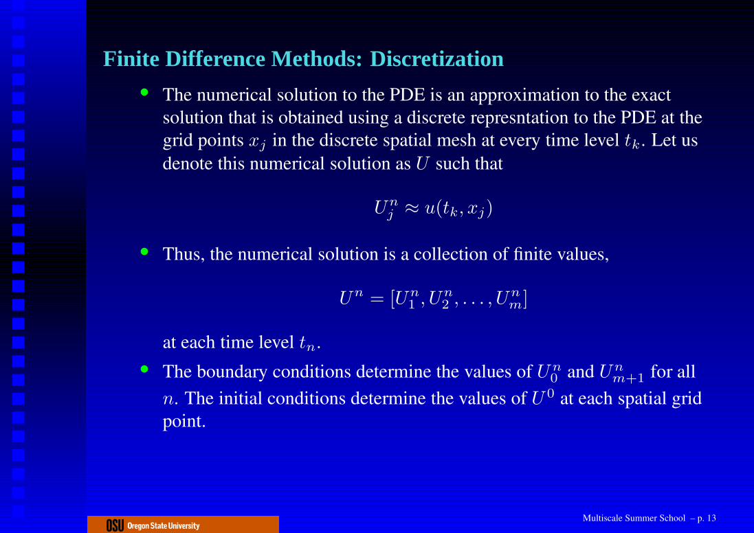
Finite Difference Methods: Discretization• The numerical solution to the PDE is an approximation to the exact
solution that is obtained using a discrete represntation to the PDE at thegrid points xj in the discrete spatial mesh at every time level tk. Let usdenote this numerical solution as U such that
Unj ≈ u(tk, xj)
• Thus, the numerical solution is a collection of finite values,
Un = [Un1 , Un
2 , . . . , Unm]
at each time level tn.• The boundary conditions determine the values of Un
0 and Unm+1 for all
n. The initial conditions determine the values of U 0 at each spatial gridpoint.
Multiscale Summer School – p. 13

Finite Difference Methods: Discretization• The numerical solution to the PDE is an approximation to the exact
solution that is obtained using a discrete represntation to the PDE at thegrid points xj in the discrete spatial mesh at every time level tk. Let usdenote this numerical solution as U such that
Unj ≈ u(tk, xj)
• Thus, the numerical solution is a collection of finite values,
Un = [Un1 , Un
2 , . . . , Unm]
at each time level tn.
• The boundary conditions determine the values of Un0 and Un
m+1 for alln. The initial conditions determine the values of U 0 at each spatial gridpoint.
Multiscale Summer School – p. 13
Finite Difference Methods: Discretization• The numerical solution to the PDE is an approximation to the exact
solution that is obtained using a discrete represntation to the PDE at thegrid points xj in the discrete spatial mesh at every time level tk. Let usdenote this numerical solution as U such that
Unj ≈ u(tk, xj)
• Thus, the numerical solution is a collection of finite values,
Un = [Un1 , Un
2 , . . . , Unm]
at each time level tn.• The boundary conditions determine the values of Un
0 and Unm+1 for all
n. The initial conditions determine the values of U 0 at each spatial gridpoint.
Multiscale Summer School – p. 13

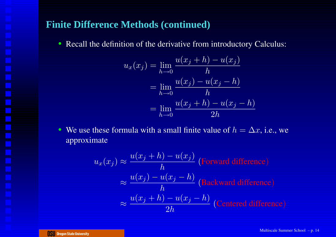
Finite Difference Methods (continued)
• Recall the definition of the derivative from introductory Calculus:
ux(xj) = limh→0
u(xj + h) − u(xj)
h
= limh→0
u(xj) − u(xj − h)
h
= limh→0
u(xj + h) − u(xj − h)
2h
• We use these formula with a small finite value of h = ∆x, i.e., weapproximate
ux(xj) ≈u(xj + h) − u(xj)
h(Forward difference)
≈u(xj) − u(xj − h)
h(Backward difference)
≈u(xj + h) − u(xj − h)
2h(Centered difference)
Multiscale Summer School – p. 14

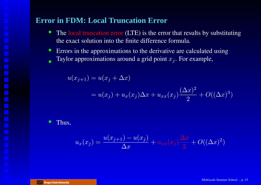
Error in FDM: Local Truncation Error• The local truncation error (LTE) is the error that results by substituting
the exact solution into the finite difference formula.
• Errors in the approximations to the derivative are calculated usingTaylor approximations around a grid point xj . For example,•
u(xj+1) = u(xj + ∆x)
= u(xj) + ux(xj)∆x + uxx(xj)(∆x)2
2+ O((∆x)3)
• Thus,
ux(xj) =u(xj+1) − u(xj)
∆x+ uxx(xj)
∆x
2+ O((∆x)2)
• The forward difference is a first order accurate approximation to thepartial derivative ux at xj and the LTE is O(∆x).
Multiscale Summer School – p. 15

Error in FDM: Local Truncation Error• The local truncation error (LTE) is the error that results by substituting
the exact solution into the finite difference formula.• Errors in the approximations to the derivative are calculated using
Taylor approximations around a grid point xj . For example,
•
u(xj+1) = u(xj + ∆x)
= u(xj) + ux(xj)∆x + uxx(xj)(∆x)2
2+ O((∆x)3)
• Thus,
ux(xj) =u(xj+1) − u(xj)
∆x+ uxx(xj)
∆x
2+ O((∆x)2)
• The forward difference is a first order accurate approximation to thepartial derivative ux at xj and the LTE is O(∆x).
Multiscale Summer School – p. 15

Error in FDM: Local Truncation Error• The local truncation error (LTE) is the error that results by substituting
the exact solution into the finite difference formula.• Errors in the approximations to the derivative are calculated using
Taylor approximations around a grid point xj . For example,•
u(xj+1) = u(xj + ∆x)
= u(xj) + ux(xj)∆x + uxx(xj)(∆x)2
2+ O((∆x)3)
• Thus,
ux(xj) =u(xj+1) − u(xj)
∆x+ uxx(xj)
∆x
2+ O((∆x)2)
• The forward difference is a first order accurate approximation to thepartial derivative ux at xj and the LTE is O(∆x).
Multiscale Summer School – p. 15

Error in FDM: LTE
• The backward difference is a first order accurateapproximation to the partial derivative ux at xj and the LTEis O(∆x).
• The centered difference is a second order accurateapproximation to the partial derivative ux at xj and the LTEis O((∆x)2).
• Note that the LTE in all these approximations goes to zeroas ∆x goes to zero.
Multiscale Summer School – p. 16

FDM for Parabolic PDEs: The Heat Equation
• Consider the initial-boundary value problem for the heat equation
ut = κuxx, 0 ≤ x ≤ 1, t ≥ 0
u(0, x) = f(x), Initial Condition
u(t, 0) = α, Boundary Condition at x = 0
u(t, 1) = β, Boundary Condition at x = 1
• Discretize the spatial domain [0, 1] into m + 2 grid points using auniform mesh step size ∆x = 1/(m + 1) . Denote the spatial gridpoints by xj , j = 0, 1, . . .m + 1.
-
-∆x
xq q q q q q q q q q q
0 = x0 x1 x2 . . . . . . xj−1 xj xj+1 . . . xm xm+1 = 1
Multiscale Summer School – p. 17

FDM for Parabolic PDEs: The Heat Equation
• Similarly discretize the temporal domain into temporal grid pointstk = k∆t for suitably chosen time step ∆t.
• Denote the approximate solution at the grid point (tk, xj) as Ukj .
-
-∆x
xq q q q q q q q q q q
0 = x0 x1 x2
α = uk0
tk = k∆tuk1 uk
2
. . . . . . xj−1 xj xj+1
ukj−1 uk
j ukj+1
. . . xm xm+1 = 1
ukm
ukm+1 = β
• The space-time grid can be represented as
(t2, xj)
66
- x6
6?
∆t
t
q q q q q q q q q q q
q q q q q q q q q q q
q q q q q q q q q q q
q q q q q q q q q q q
0 = x0 x1 x2 . . . . . . xj−1 xj xj+1 . . . xm xm+1 = 1
t0
t1
t2
...
Multiscale Summer School – p. 18

FDM for Parabolic PDEs: The Heat Equation
• Replace ut by a forward difference in time and uxx by a centraldifference in space to obtain the explicit FDM
•
Uk+1j − Uk
j
∆t= κ
Ukj+1 − 2Uk
j + Ukj−1
(∆x)2
=⇒ Uk+1j = Uk
j +κ∆t
(∆x)2(
Ukj+1 − 2Uk
j + Ukj−1
)
, j = 1, 2, . . .m
• Associated to this scheme is a Computational Stencil
q q q
q q q
q q q
6
@
@@I
j − 1 j j + 1
k − 1
k
k + 1
Multiscale Summer School – p. 19

FDM for Parabolic PDEs: The Heat Equation
• This is an explicit FDM for the heat equation: Solution at time levelk + 1 is determined by solution at previous time levels only.
• We note that• From Boundary conditions: Uk
0 = α and Ukm+1 = β for all values
of k.• From Initial condition: U 0
j = f(xj) for all values of j.
• The local truncation error is O(∆t) + O((∆x)2).Scheme is first order accurate in time and second order accurate in space
• How do we choose the values of ∆t and ∆x??
Multiscale Summer School – p. 20

FDM for Parabolic PDEs: The Heat Equation
• This is an explicit FDM for the heat equation: Solution at time levelk + 1 is determined by solution at previous time levels only.
• We note that• From Boundary conditions: Uk
0 = α and Ukm+1 = β for all values
of k.• From Initial condition: U 0
j = f(xj) for all values of j.• The local truncation error is O(∆t) + O((∆x)2).
Scheme is first order accurate in time and second order accurate in space
• How do we choose the values of ∆t and ∆x??
Multiscale Summer School – p. 20

FDM for Parabolic PDEs: The Heat Equation
0 0.2 0.4 0.6 0.8 10
0.1
0.2
0.3
0.4
0.5
0.6
0.7
0.8
0.9
1
dx=0.01, dt=1e−05, r=0.1
ExactSolution
Initialfunction
• Initial condition has a discontinuous derivative at x = 0.5.
Multiscale Summer School – p. 21

FDM for Parabolic PDEs: The Heat Equation
• Initial condition has a discontinuous derivative at x = 0.5.
• However, we see a rapid smoothing effect of this initial discontinuity astime evolves.
• In general high frequencies get rapidly damped as compared to lowfrequencies. We say that the heat equation is stiff.
• In the above we assumed that the value of
r =κ∆t
∆x≤
1
2
Here ∆x = 0.01 and ∆t = 10−5
• What happens if this value is greater than 1/2?
Multiscale Summer School – p. 22

FDM for Parabolic PDEs: The Heat Equation
• Initial condition has a discontinuous derivative at x = 0.5.• However, we see a rapid smoothing effect of this initial discontinuity as
time evolves.
• In general high frequencies get rapidly damped as compared to lowfrequencies. We say that the heat equation is stiff.
• In the above we assumed that the value of
r =κ∆t
∆x≤
1
2
Here ∆x = 0.01 and ∆t = 10−5
• What happens if this value is greater than 1/2?
Multiscale Summer School – p. 22

FDM for Parabolic PDEs: The Heat Equation
• Initial condition has a discontinuous derivative at x = 0.5.• However, we see a rapid smoothing effect of this initial discontinuity as
time evolves.• In general high frequencies get rapidly damped as compared to low
frequencies. We say that the heat equation is stiff.
• In the above we assumed that the value of
r =κ∆t
∆x≤
1
2
Here ∆x = 0.01 and ∆t = 10−5
• What happens if this value is greater than 1/2?
Multiscale Summer School – p. 22

FDM for Parabolic PDEs: The Heat Equation
• Initial condition has a discontinuous derivative at x = 0.5.• However, we see a rapid smoothing effect of this initial discontinuity as
time evolves.• In general high frequencies get rapidly damped as compared to low
frequencies. We say that the heat equation is stiff.• In the above we assumed that the value of
r =κ∆t
∆x≤
1
2
Here ∆x = 0.01 and ∆t = 10−5
• What happens if this value is greater than 1/2?
Multiscale Summer School – p. 22

FDM for Parabolic PDEs: The Heat Equation
0 0.2 0.4 0.6 0.8 1−1.5
−1
−0.5
0
0.5
1
1.5x 10
282
dx=0.01, dt=0.0001, r=1
• We see unstable behavior of the numerical solution! The numericalsolution does not stay bounded.
• Thus, ∆t and ∆x cannot be chosen arbitrarily. They have to satisfy astability condition.
Multiscale Summer School – p. 23
Implicit FDM for Parabolic PDEs: The Heat Equation
• Replace ut by a forward difference in time and uxx by a centraldifference in space to obtain the Implicit FDM
•
Uk+1j − Uk
j
∆t= κ
Uk+1j+1 − 2Uk+1
j + Uk+1j−1
(∆x)2
=⇒ Uk+1j = Uk
j +κ∆t
(∆x)2(
Uk+1j+1 − 2Uk+1
j + Uk+1j−1
)
, j = 1, 2, . . .m
• Associated to this scheme is a Computational Stencil
q q q
q q q
q q q
6
j − 1 j j + 1
k − 1
k
k + 1
Multiscale Summer School – p. 24
FDM for Parabolic PDEs: The Heat Equation
0 0.2 0.4 0.6 0.8 10
0.1
0.2
0.3
0.4
0.5
0.6
0.7
0.8
0.9
1
dx=0.01, dt=0.01, r=100
Initialfunction
ExactSolution
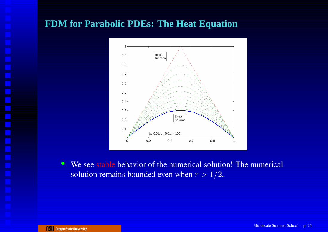
• We see stable behavior of the numerical solution! The numericalsolution remains bounded even when r > 1/2.
• Thus, ∆t and ∆x can be chosen to have the same order of magnitude.• The implicit FDM is unconditionally stable• However, the implicit scheme is still first order accurate in time and
second order accurate in space. Also, a system of equations must besolved at each step.
Multiscale Summer School – p. 25
FDM for Parabolic PDEs: The Heat Equation
0 0.2 0.4 0.6 0.8 10
0.1
0.2
0.3
0.4
0.5
0.6
0.7
0.8
0.9
1
dx=0.01, dt=0.01, r=100
Initialfunction
ExactSolution
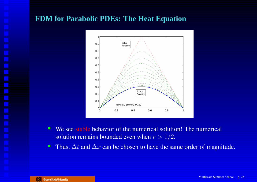
• We see stable behavior of the numerical solution! The numericalsolution remains bounded even when r > 1/2.
• Thus, ∆t and ∆x can be chosen to have the same order of magnitude.
• The implicit FDM is unconditionally stable• However, the implicit scheme is still first order accurate in time and
second order accurate in space. Also, a system of equations must besolved at each step.
Multiscale Summer School – p. 25
FDM for Parabolic PDEs: The Heat Equation
0 0.2 0.4 0.6 0.8 10
0.1
0.2
0.3
0.4
0.5
0.6
0.7
0.8
0.9
1
dx=0.01, dt=0.01, r=100
Initialfunction
ExactSolution
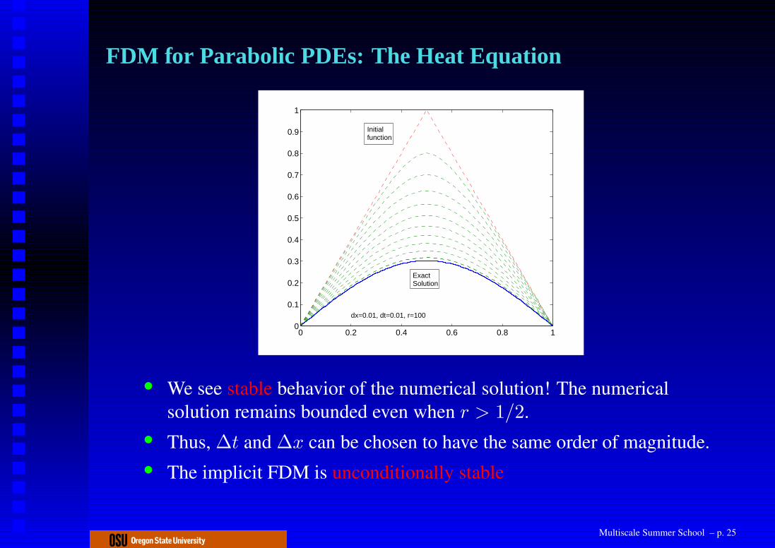
• We see stable behavior of the numerical solution! The numericalsolution remains bounded even when r > 1/2.
• Thus, ∆t and ∆x can be chosen to have the same order of magnitude.• The implicit FDM is unconditionally stable
• However, the implicit scheme is still first order accurate in time andsecond order accurate in space. Also, a system of equations must besolved at each step.
Multiscale Summer School – p. 25

Crank-Nicolson for The Heat Equation
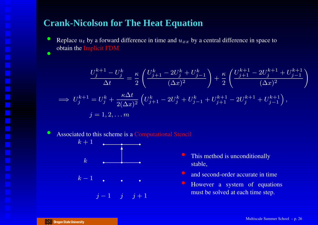
• Replace ut by a forward difference in time and uxx by a central difference in space toobtain the Implicit FDM
•
Uk+1j − Uk
j
∆t=
κ
2
Ukj+1 − 2Uk
j + Ukj−1
(∆x)2
!
+κ
2
Uk+1j+1 − 2Uk+1
j + Uk+1j−1
(∆x)2
!
=⇒ Uk+1j = Uk
j +κ∆t
2(∆x)2
“
Ukj+1 − 2Uk
j + Ukj−1 + Uk+1
j+1 − 2Uk+1j + Uk+1
j−1
”
,
j = 1, 2, . . . m
• Associated to this scheme is a Computational Stencil
q q q
q q q
q q q
6
j − 1 j j + 1
k − 1
k
k + 1
• This method is unconditionallystable,
• and second-order accurate in time• However a system of equations
must be solved at each time step.
Multiscale Summer School – p. 26

Crank-Nicolson for The Heat Equation
• Replace ut by a forward difference in time and uxx by a central difference in space toobtain the Implicit FDM
•
Uk+1j − Uk
j
∆t=
κ
2
Ukj+1 − 2Uk
j + Ukj−1
(∆x)2
!
+κ
2
Uk+1j+1 − 2Uk+1
j + Uk+1j−1
(∆x)2
!
=⇒ Uk+1j = Uk
j +κ∆t
2(∆x)2
“
Ukj+1 − 2Uk
j + Ukj−1 + Uk+1
j+1 − 2Uk+1j + Uk+1
j−1
”
,
j = 1, 2, . . . m
• Associated to this scheme is a Computational Stencil
q q q
q q q
q q q
6
j − 1 j j + 1
k − 1
k
k + 1
• This method is unconditionallystable,
• and second-order accurate in time• However a system of equations
must be solved at each time step.
Multiscale Summer School – p. 26

First vs Second Order Accuracy
−14 −12 −10 −8 −6 −4 −2 0−14
−12
−10
−8
−6
−4
−2
0
log2(∆ x)
log 2(L
TE
)
Slope =1: Firstorder accurate
Slope =2: SecondOrder accurate
Multiscale Summer School – p. 27

Method of Lines (MOL) Discretization
• Another way of solving time dependent PDEs numericallyis to discretize in space but not in time.
• This results in a large coupled system of ODEs which wecan then solve using numerical methods developed forODEs, such as Forward and Backward Euler method,Trapedoizal methods, Runge-Kutta methods etc.
• The method of lines approach can be used to analyze thestability of the numerical method for the PDE by analyzingthe eigenvalues of the matrix of the resulting system ofODEs using the ideas of absolute stability for ODEs.
Multiscale Summer School – p. 28

Analysis of FDM
• Consitency implies that the local truncation error goes to zero as ∆xand ∆t approach zero. This is usually proved by invoking Taylor’stheorem.
• Stability implies that the numerical solution remains bounded at anygiven time t. Stability is harder to prove than consistency. Stability canbe proven using either• Eigenvalue analysis of the matrix representation of the FDM.• Fourier analysis on the grid (von Neumann analysis)• Computing the domain of dependence of the numerical method.
• Lax-Equivalence Theorem : A consistent approximation to awell-posed problem is convergent if and only if it is stable
Multiscale Summer School – p. 29

Von Neumann Analysis for Time-dependent Problems• Example: The analytical solutions of the heat equation ut − κuxx = 0
can be found in the form
u(t, x) =∞∑
−∞
eβmteiαmx
with βm + κα2m = 0. Here eiαmx = cos(αmx) + i sin(αmx).
• To analyze the growth of different Fourier modes as they evolve underthe numerical scheme we consider each frequency separately, namelylet u(t, x) = eβmteiαmx
• In the discrete case we assume that Ukj = Gkeiαmj∆x with
G = eβm∆t. Any growth in the solution will be due to the presence ofterms involving G.
• Thus requiring that this amplification factor G is bounded by one ask → ∞ gives rise to a relation between ∆t and ∆x called the vonNeumann stability condition.
Multiscale Summer School – p. 30

FDM for Hyperbolic PDEs: The Advection Equation
• Consider the initial value problem for the Advection equation
ut + aκux = 0, 0 ≤ x ≤ 1, t ≥ 0
u(0, x) = f(x), Initial Condition
• The solution u(x, t) = f(x − at) is a wave that propagates to the rightif a > 0 and to the left if a < 0.
x
x
t
u (x,0 )
u (x,t ) C h a ra cte ris ticx a t c
• Information propagates along characteristics
Multiscale Summer School – p. 31

FDM for the Advection Equation
• Replace ut by a forward difference in time and ux by a backwarddifference in space to obtain the explicit FDM
•
Uk+1j − Uk
j
∆t+ a
Ukj+1 − Uk
j
∆x= 0
=⇒ Uk+1j = Uk
j +a∆t
∆x
(
Ukj − Uk
j−1
)
, j = 1, 2, . . .m
• Associated to this scheme is a Computational Stencil
q q q
q q q
q q q
6
j − 1 j j + 1
k − 1
k
k + 1 • Scheme is explicit• First order accurate is time
and space• ∆t and ∆x are related
through the Courant number
ν =a∆t
∆x
Multiscale Summer School – p. 32

Courant Friedrich Lewy (CFL) Condition
• The CFL Condition : For stability, at each mesh point, the Domain ofdepencence of the PDE must lie within the domain of dependence ofthe numerical scheme.
P
Q
P
(a) (b )
C h arac te ris tic
Q
∆ t∆ t
a ∆ t
a ∆ t
t
x
∆ x ∆ xt
x
• CFL is a necessary condition for stability of explicit FDM applied toHyperbolic PDEs. It is not a sufficient condition.
• For the advection equation CFL condition for stability is |ν| ≤ 1. i.e.,
∆t ≤∆x
|a|.
Multiscale Summer School – p. 33

Elliptic PDEs: Laplace Equation
• Time-independent problems
• Consider the Boundary value problem for Laplace equation in twospatial dimensions
uxx + uyy = 0, 0 ≤ x ≤ 1, 0 ≤ y ≤ 1
with boundary conditions prescibed as shown below
6
- x
u = 0
u = 1
u = 0 u = 0
y
Multiscale Summer School – p. 34

Elliptic PDEs: Laplace Equation
• Time-independent problems• Consider the Boundary value problem for Laplace equation in two
spatial dimensions
uxx + uyy = 0, 0 ≤ x ≤ 1, 0 ≤ y ≤ 1
with boundary conditions prescibed as shown below
6
- x
u = 0
u = 1
u = 0 u = 0
y
Multiscale Summer School – p. 34

FDM for Elliptic PDEs: Laplace Equation
• Discretize the mesh using uniform mesh step in both the x and ydirections as below.
6? -
- x6y
t t t t t t t t t t t
t t t t t t t t t t
t t t t t t t t t t
t t t t t t t t t t
t t t t t t t t t t
t t t t t t t t t t
t t t t t t t t t t
t t t t t t t t t t t
t
t
t
t
t
t
t
t
t
t
t
t
t
t
t
t
0 = x0 x1 x2 . . . . . . xj−1 xj xj+1 . . . xm xm+1 = 1
0 = y0
y1
y2
...
...
ym−1
ym
ym+1 = 1
∆x
∆y
Multiscale Summer School – p. 35

Elliptic PDEs: Laplace Equation
• Replace both the second order derivatives uxx and uyy with centereddifferences at each grid point (xj , yk) to obtain the difference scheme
Uj+1,k − 2Uj,k + Uj−1,k
(∆x)2+
Uj,k+1 − 2Uj,k + Uj,k−1
(∆y)2= 0
• If ∆x = ∆y this becomes
Uj+1,k + Uj−1,k + Uj,k+1 + Uj,k−1 − 4Uj,k = 0
• The Stencil for this FDM is called the Five-Point Stencil
q q q
q q q
q q q
j − 1 j j + 1
k − 1
k
k + 1
Multiscale Summer School – p. 36

Elliptic PDEs: Laplace Equation
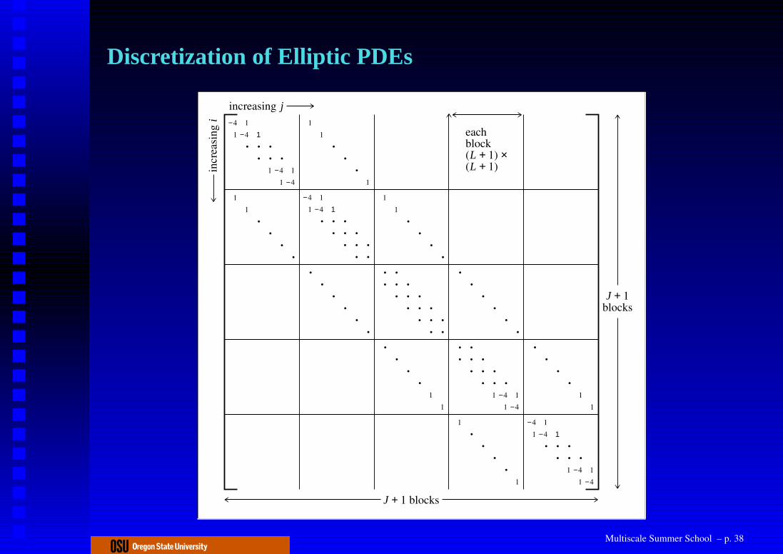
• This FDM gives rise to a system of linear equations of the form
AU = b
• The right hand side vector b contains the boundary information.• The vector U is the solution vector at the interior grid points.• The matrix A is block tridiagonal if ordered in a natural way• The structure of A depends on the ordering of the grid points.• This system can be solved by iterative techniques or direct
methods such as Gaussian elimination.
• When m = 2, the system AU = b can be written as
−4 1 1 0
1 −4 0 1
1 0 −4 1
0 1 1 −4
U1,1
U2,1
U1,2
U2,2
=
0
0
1
1
Multiscale Summer School – p. 37

Elliptic PDEs: Laplace Equation
• This FDM gives rise to a system of linear equations of the form
AU = b
• The right hand side vector b contains the boundary information.• The vector U is the solution vector at the interior grid points.• The matrix A is block tridiagonal if ordered in a natural way• The structure of A depends on the ordering of the grid points.• This system can be solved by iterative techniques or direct
methods such as Gaussian elimination.• When m = 2, the system AU = b can be written as
−4 1 1 0
1 −4 0 1
1 0 −4 1
0 1 1 −4
U1,1
U2,1
U1,2
U2,2
=
0
0
1
1
Multiscale Summer School – p. 37
Discretization of Elliptic PDEs
−41
1−4
•1••
••1
•−4
11
−4
J + 1blocks
incr
easin
gi
increasing j
J + 1 blocks
11
••
••
−41
1−4
•1••
•••
•••
••
••
•••
•••
•••
•••
••
••
•••
•••
••1
•−4
11
−4
−41
1−4
•1••
••1
•−4
11
−4
••
••
••
1•
••
•1
••
••
11
11
••
•1
••
••
••
11
••
••
••
••
11
eachblock(L + 1) ×(L + 1)
Multiscale Summer School – p. 38

Finite Element MethodFeatures
• Flexibility• Complicated geometries• High-order approximations• Strong mathematical foundation
Multiscale Summer School – p. 39

Basic Idea
u(x) ≈ u(x) =M
∑
j=1
ujφj(x)
• φj are basis functions• uj: M unknowns; Need M equations• Discretizing derivatives results in linear system
Multiscale Summer School – p. 40

1D Elliptic Example
−u′′ = f, 0 < x < 1
u(0) = u(1) = 0
• For example, elastic cord with fixed ends• Solution must be twice differentiable• This is unnecessarily strong if f is discontinuous
Multiscale Summer School – p. 41

Weak FormulationMultiply both sides by an arbitrary test function v andintegrate
∫ 1
0
−u′′vdx =
∫ 1
0
fvdx
∫ 1
0
u′v′dx − u′v|10 =
∫ 1
0
fvdx.
∫ 1
0
u′v′dx =
∫ 1
0
fvdx.
Since v was arbitrary, this equation must hold for all v
such that the equation makes sense (v′ is squareintegrable), and v(0) = v(1) = 0.
Multiscale Summer School – p. 42

Weak Formulation 2Find u ∈ V such that
∫ 1
0
u′v′dx =
∫ 1
0
fvdx ∀v ∈ V
where V = H10([0, 1]).
• Fewer derivatives required for u
• If f continuous, same u as strong form• Infinite possibilities for v
• Want to find u on a discrete mesh
Multiscale Summer School – p. 43

Finite-dimensional Subspace• Let 0 = x0 < x1 < . . . < xM+1 = 1 be a partition
of the domain with hj = xj − xj−1 andh = max hj. Use the partition to define afinite-dimensional subspace Vh ⊂ V .
• For decreasing h, want that functions in Vh canget arbitrarily close to functions in V .
• For example, let Vh be piecewise linear (i.e., oneach subinterval) functions such that v ∈ Vh iscontinuous on [0, 1] and v(0) = v(1) = 0.
• We may introduce basis functions φj(x) such thatφj(xi) = δij for i, j = 0, . . . ,M + 1.
• Nodes xi are sometimes denoted Ni
Multiscale Summer School – p. 44

Basis FunctionsFinite methods for partial differential equations 19
...
x
1
...
Ni (x)
Ωi
x
x
1
x
1
u1
x1
ui
uN
xNxi
ui 1
ui 1
u1 x
ui x
uN x
xi 1xi 1
∑
Multiscale Summer School – p. 45

Finite Element MethodFind u ∈ Vh such that
∫ 1
0
u′v′dx =
∫ 1
0
fvdx ∀v ∈ Vh.
or∫ 1
0
u′φ′jdx =
∫ 1
0
fφjdx j = 1, . . . ,M.
Note:• When u and v in same subspace: Galerkin• If support of φi is entire space: Spectral• If Vh not a subspace of V : Non-conforming
Multiscale Summer School – p. 46

Linear System• Can represent u =
∑Mi=1 ξiφi(x)
• Find ξi for i = 1, . . . ,M such that∫ 1
0
M∑
i=1
ξiφ′iφ
′jdx =
∫ 1
0
fφjdx j = 1, . . . ,M.
• Thus if A = (aij) with aij =∫ 1
0 φ′iφ
′jdx and
b = (bi) with bi =∫ 1
0 fφidx, then
Aξ = b
Multiscale Summer School – p. 47

Stiffness Matrix• The M × M matrix A is called the stiffness
matrix.• For the piecewise linear basis functions we have
chosen it will be tridiagonal.• For the special case when hj ≡ h we have
1
h
2 −1 0 · · · · · · 0
−1 2 −1 . . . ...0 −1 2 −1 . . . ...... . . . . . . . . . . . . 0... . . . −1 2 −1
0 · · · · · · 0 −1 2
Multiscale Summer School – p. 48

Compare to FDM• Note that if Trapezoid rule is used to approximate
the right hand side, then bi = hfi, and thereforethe equations determining u are
ξi+1 − 2ξi + ξi−1
h= hfi
which are exactly the same as FDM.• The advantage of the FEM formulation is the
generality it allows (e.g., uniform h was notrequired).
Multiscale Summer School – p. 49

Multidimensional Problem• Let Ω be the unit square (x, y) ∈ [0, 1] × [0, 1]
• Assume homogeneous Dirichlet boundaryconditions
• Then the 2D Possion problem is:Find u ∈ V := H1
0(Ω) such that
−∆u = f in Ω,
u = 0 on ∂Ω.
Multiscale Summer School – p. 50

Variational FormulationFind u ∈ V such that
a(u, v)Ω = (f, v)Ω, ∀v ∈ V,
where
a(u, v)Ω :=
∫
Ω
∇u · ∇v,
(f, v)Ω :=
∫
Ω
fv.
Note: used Green’s formula and v = 0 on ∂Ω.
Multiscale Summer School – p. 51

P1 Finite ElementWe introduce a triangulation Th of Ω into triangles Ki,and a finite dimensional subspace:
Vh := v ∈ H10(Ω) : v|Ki
∈ P1(Ki).
Find u ∈ Vh such that
a(u, v)Ω = (f, v)Ω, ∀v ∈ Vh.
Multiscale Summer School – p. 52

Using Basis FunctionsRepresenting u and v in terms of nodal basis functionsφi
Mi=1 of Vh, i.e., φj(Ni) = δij for
i, j = 0, . . . ,M + 1, we get the following system ofalgebraic equations:
M∑
j=1
ξja(φi, φj) = (f, φi), i = 1, . . . ,M,
or in matrix form,Aξ = b,
where ξj = u(Nj), Aij = a(φi, φj)Ω is SPD, andbi = (f, φi)Ω.
Multiscale Summer School – p. 53

Multidimensional Problem• Let Ω be the unit cube x, y, z ∈ [0, 1]
• Assume homogeneous Dirichlet boundaryconditions
• Then the 3D Possion problem is:Find u ∈ V := H1
0(Ω) such that
−∆u = f in Ω,
u = 0 on ∂Ω.
Multiscale Summer School – p. 54

Variational FormulationFind u ∈ V such that
a(u, v)Ω = (f, v)Ω, ∀v ∈ V,
where
a(u, v)Ω :=
∫
Ω
∇u · ∇v,
(f, v)Ω :=
∫
Ω
fv.
Note: used Green’s formula and v = 0 on ∂Ω.
Multiscale Summer School – p. 55

Q1 Finite ElementWe introduce a triangulation Th of Ω into 3-Drectangles Ki, and a finite dimensional subspace:
Vh := v ∈ H10(Ω) : v|Ki
∈ Q1(Ki).
Find u ∈ Vh such that
a(u, v)Ω = (f, v)Ω, ∀v ∈ Vh.
Multiscale Summer School – p. 56

Using Basis FunctionsRepresenting u and v in terms of nodal basis functionsφi
Mi=1 of Vh, i.e., φj(Ni) = δij for
i, j = 0, . . . ,M + 1, we get the following system ofalgebraic equations:
M∑
j=1
ξja(φi, φj) = (f, φi), i = 1, . . . ,M,
or in matrix form,Aξ = b,
where ξj = u(Nj), Aij = a(φi, φj)Ω is SPD, andbi = (f, φi)Ω.
Multiscale Summer School – p. 57

Neumann Problem• Let Ω be the unit square (x, y) ∈ [0, 1] × [0, 1]
• Assume Neumann boundary conditions• Then the 2D Possion problem is:
Find u ∈ V := H1(Ω) such that
−∆u = f in Ω,
∂u
∂n= g on ∂Ω.
Multiscale Summer School – p. 58

Variational FormulationFind u ∈ V such that
a(u, v)Ω = (f, v)Ω + 〈g, v〉∂Ω, ∀v ∈ V,
where
a(u, v)Ω :=
∫
Ω
∇u · ∇v,
(f, v)Ω :=
∫
Ω
fv,
〈g, v〉∂Ω :=
∫
∂Ω
gv.
Note: used Green’s formula and ∂u∂n = g on ∂Ω.
Multiscale Summer School – p. 59

P1 Finite ElementWe introduce a triangulation Th of Ω into triangles Ki,and a finite dimensional subspace:
Vh := v ∈ H1(Ω) : v|Ki∈ P1(Ki).
Find u ∈ Vh such that
a(u, v)Ω = (f, v)Ω + 〈g, v〉∂Ω, ∀v ∈ Vh.
Multiscale Summer School – p. 60

Using Basis FunctionsRepresenting u and v in terms of nodal basis functionsφi
M+1i=0 of Vh, we get the following system of
algebraic equations:
M+1∑
j=0
ξja(φi, φj) = (f, φi)+〈g, φi〉∂Ω, i = 0, . . . ,M+1,
or in matrix form,Aξ = b,
where ξj = u(Nj), Aij = a(φi, φj)Ω is SPD, andbi = (f, φi)Ω + 〈g, φi〉∂Ω.
Multiscale Summer School – p. 61

Mixed BoundaryLet Ω be the unit cube, Γ0 the face at z = 0, andΓ1 = ∂Ω \ Γ0. Then we want to approximate u in Ω.
Γ0
Γ1
Ω
Multiscale Summer School – p. 62

Mixed Robin BoundaryFind u ∈ V := H1(Ω) such that
−∆u = f in Ω,
α0u + β0∂u
∂n= 0 on Γ0,
α1u + β1∂u
∂n= 0 on Γ1.
Note: assume βi 6= 0.
Multiscale Summer School – p. 63

Variational FormulationFind u ∈ V such that
a(u, v)Ω −
⟨
∂u
∂n, v
⟩
Γ0
−
⟨
∂u
∂n, v
⟩
Γ1
= (f, v)Ω,
or
a(u, v)Ω + α0β−10 〈u, v〉Γ0
+ α1β−11 〈u, v〉Γ1
= (f, v)Ω,
where a(u, v)Ω and (f, v)Ω are the same as above and
〈u, v〉Γj:=
∫
Γj
uv, j = 0, 1.
Multiscale Summer School – p. 64

Finite Element MethodWe introduce the triangulation Th as before, and thefinite dimensional subspace
Vh := u ∈ H1(Ω) : u|Ki∈ Q1(Ki)
to get the finite element problem:Find u ∈ Vh such that
a(u, v)Ω + α0β−10 〈u, v〉Γ0
+ α1β−11 〈u, v〉Γ1
= (f, v)Ω, ∀v ∈ Vh.
Multiscale Summer School – p. 65

Using Basis FunctionsRepresenting u and v in terms of nodal basis functionsφi
Mi=1 of Vh we get the following matrix equation:
(A + G)ξ = b,
where ξ, A, and b are similar to those above and
G0ij := 〈φi, φj〉Γ0
,
G1ij := 〈φi, φj〉Γ1
,
G :=α0
β0G0 +
α1
β1G1.
Multiscale Summer School – p. 66

Parabolic and Elliptic• Build off of elliptic FEM• If boundary not moving, space-time rectangular
in t dimension• Popular to use FEM for spatial discretization and
FDM for time• Performing FEM first results in semi-discrete
formulation• This is equivalent to a coupled system of ODEs
Multiscale Summer School – p. 67

Scalar Wave ProblemFind u ∈ H2([0, T ]; L2(Ω)) ∩ L2([0, T ]; H1
0 (Ω)) suchthat
1
c2utt − ∆u = f in Ω,
u = 0 in ∂Ω × (0, T ),
u(·, 0) = u0(·) in Ω,
ut(·, 0) = u1(·) in Ω.
Multiscale Summer School – p. 68

Variational FormulationFind u(·, t) : [0, T ] → V := H1
0(Ω) such that
1
c2(utt, v)Ω + a(u, v)Ω = (f, v)Ω, ∀v ∈ V,
(u(·, 0), v)Ω = (u0(·), v)Ω, ∀v ∈ V,
(ut(·, 0), v)Ω = (u1(·), v)Ω, ∀v ∈ V.
Multiscale Summer School – p. 69

Semi-discrete FormulationFind u(·, t) : [0, T ] → Vh such that
1
c2(uh, v)Ω + a(u, v)Ω = (f, v)Ω, ∀v ∈ Vh,
(u(·, 0), v)Ω = (u0(·), v)Ω, ∀v ∈ Vh,
(uh(·, 0), v)Ω = (u1(·), v)Ω, ∀v ∈ Vh.
Multiscale Summer School – p. 70
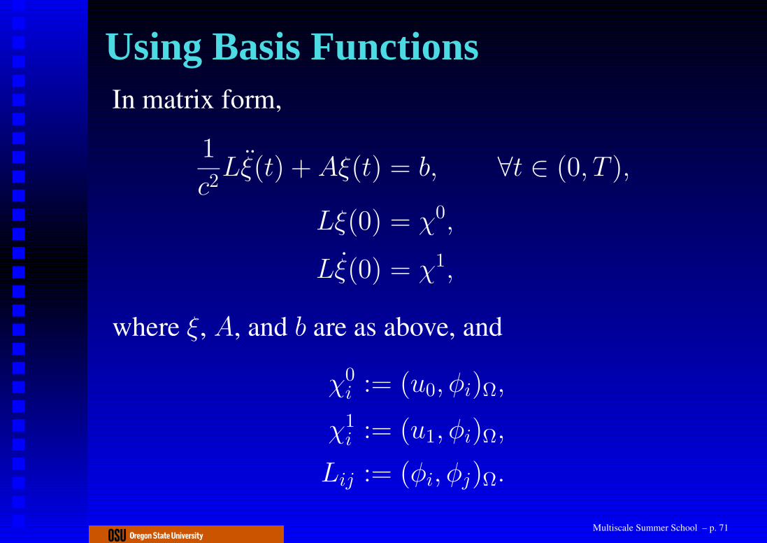
Using Basis FunctionsIn matrix form,
1
c2Lξ(t) + Aξ(t) = b, ∀t ∈ (0, T ),
Lξ(0) = χ0,
Lξ(0) = χ1,
where ξ, A, and b are as above, and
χ0i := (u0, φi)Ω,
χ1i := (u1, φi)Ω,
Lij := (φi, φj)Ω.
Multiscale Summer School – p. 71

Fully Discrete FormulationIn order to discretize in time, we introduce a(uniform) partition of the interval [0,T]:0 = t0 < t1 < · · · < tNT
= T , andk := tn − tn−1, n = 1, . . . , NT .
1
c2L
ξn+1 − 2ξn + ξn−1
k2+ Aξn = bn, n = 1, . . . , NT ,
Lξ0 = χ0,
Lξ1 = χ0 + kχ1,
where ξni ≈ ξi(tn) and bn
i := bi(tn).
Multiscale Summer School – p. 72
Mass Lumping• Note that the fully discrete formulation is still
implicit, thus a linear solve at each time step mustbe performed.
• Since Lij := (φi, φj)Ω, it is possible to make L
diagonal by using a quadrature rule (Trapezoid)for the integration.
• The resulting explicit method is exactly the FDM.• When to lump is an important question;
numerical dispersion analysis can show, forexample, in 1D consistent mass matrix requires asmaller time step than lumped, and a linear solve!
• Mass lumping can reduce accuracy, especially inhigher dimensions.
Multiscale Summer School – p. 73

Other Considerations• Integration performed in “local” coordinates, then global
matrix assembled.• K may be mapped to reference domain (e.g., [−1, 1]) for
easy integration (especially quadrature rules).• Technically speaking a finite element is a triple: geometric
object, finite-dimensional linear function space, and a set ofdegrees of freedom.
• Many types of finite elements exist, including some withquadratic or cubic basis functions, first or second derivativesas degrees of freedom, or degrees of freedom in locationsother than vertices (e.g., centroid).
• More general than FDM, and more easily applied to slantedor curved boundaries, especially involving normal derivativeboundary conditions.
Multiscale Summer School – p. 74

Conservation Laws• Many PDEs are derived from physical models
called conservation laws.• The general principle is that the rate of change of
u(x, t) within a volume V is equal to the flux pastthe boundary
∂
∂t
∫
V
u(x, t) +
∫
∂V
f(u) · n = 0
where f is flux function.• Nonlinear conservation laws can result in
discontinuities in finite time even with smoothinitial data.
Multiscale Summer School – p. 75

Finite Volume Method• Rather than pointwise approximations on a grid, FVM
approximates the average integral value on a referencevolume.
• Suppose region Vi = [xi−(1/2), xi+(1/2)] then∫ xi+(1/2)
xi−(1/2)
utdx + f(ui+(1/2)) − f(ui−(1/2)) = 0
where we have applied Gauss’s theorem and integratedanalytically the resulting term
∫ xi+(1/2)
xi−(1/2)fx(u)dx.
• We can apply a quadrature rule, for example Midpoint, tothe remaining integral to get a semi-discrete form(
xi+(1/2) − xi−(1/2)
)
ut(xi) + f(ui+(1/2)) − f(ui−(1/2)) = 0.
Multiscale Summer School – p. 76

FVM Example
Consider the elliptic equation uxx = f(x) on a control volumeVi = [xi−(1/2), xi+(1/2)] then
∫ xi+(1/2)
xi−(1/2)
uxxdx =
∫ xi+(1/2)
xi−(1/2)
fdx.
Evaluating the left hand side analytically and the right viaMidpoint gives
ux(xi+(1/2)) − ux(xi−(1/2)) =(
xi+(1/2) − xi−(1/2)
)
fi
Finally, using centered differences on the remaining derivativesyields
ui+1 − 2ui + ui−1
h= hfi
for h = xi+(1/2) − xi−(1/2).
Multiscale Summer School – p. 77

FVM Summary• Applies to integral form of conservation law.• Handles discontinuities in solutions.• Natural choice for heterogeneous material as each
grid cell can be assigned different materialparameters.
• There exist theory for convergence, accuracy andstability.
Multiscale Summer School – p. 78

Systems of Linear Equations• For implicit methods must choose a linear solver.• Direct (LU factorization)
• More accurate• May be cheaper for many time steps• Banded (otherwise fill-in)
• Iterative• If accuracy less important than speed• Matrix-free• Sparse• SPD
Multiscale Summer School – p. 79

Iterative Methods• Successive Over Relaxation (SOR)
• Simple to code• ω = 1 is Gauss-Seidel
• Conjugate Gradient• SPD• Eigenvalues clustered together (Precondition)
• Generalized Minimum Residual (GMRES)• Non-SPD, e.g. convection-diffusion with
upwinding• Krylov method: builds orthonormal basis
which may get big (Restart)• Preconditioning helps (Incomplete Cholesky)
Multiscale Summer School – p. 80


![Finite Element Method - Massachusetts Institute of … · Finite Element Method January 12, 2004 ... - Solve the boundary value problem [7] Process ... Very large stiffness difference](https://static.fdocuments.net/doc/165x107/5b4f1c0a7f8b9a3e6e8ba1ea/finite-element-method-massachusetts-institute-of-finite-element-method-january.jpg)