An introduction for geoscientists - UKOGL
53
Maps and map interpretation An introduction for geoscientists Produced by the University of Derby in conjunction with UKOGL
Transcript of An introduction for geoscientists - UKOGL

Maps and map interpretation
An introduction for geoscientists
Produced by the University of Derby in conjunction with UKOGL

• This teaching package provides an introduction to maps and how to identify landforms using contours and cross-sections
• It is designed primarily for A-Level and first year undergraduate geology and geography students who may have little experience of topographic maps, or for those who haven’t worked with them recently
Aims
Presenter
Presentation Notes
If you are delivering this session to a class and want to incorporate the two practical sessions, print out multiple copies of Slides 50-52 beforehand and provide graph paper for drawing the cross-section

• Part 1 - Introduction to maps • Title • Key (sometimes called legend or explanation) • Scales • Contours
• Part 2 – Map interpretation
• Contour patterns • Cross-sections
Contents

Part 1 - Introduction to maps
• Maps are a 2-D representation of a 3-D world. They are a ‘bird’s eye’ view – as if the viewer is ‘flying’ above the land surface and looking down on it
• They show how objects are distributed and their relative size
• Maps are a very useful way of visualizing all sorts of data and they are a key tool for geoscientists

The same map outline can be used to show different information, so it is important to identify the
map title, key, scale and orientation
UK Bedrock Geology UK Annual Mean Wind Speed
N N
Title
Key
Scale
North Point
Presenter
Presentation Notes
Questions for students: Are the maps the same scale and orientation? Answer: Yes What does the key for the Bedrock Geology Map tell you? Answer: There are three groups of rocks – sedimentary, metamorphic and igneous.

Maps show how objects are distributed and their relative size
© Crown Copyright/database right 2014. An Ordnance Survey/EDINA supplied service.
N
This is the area north of Derby that we will be focusing on later
Presenter
Presentation Notes
Which is furthest west, Derby or Nottingham? Answer: Derby Which occupies the greater area, Derby or Nottingham? Answer: Nottingham

Scales • Show the distance on the map compared to the
distance on the ground • It is important to choose an appropriate map
scale for the task you are undertaking • Common scales include:
1:30 000 000 (e.g. world map or atlas) 1:1 000 000 (e.g. country map) 1:50 000 (e.g. regional map) 1:10 000 (e.g. local map)
• A map scale of 1:50 000 means: 1mm on the map represents 50 000mm or 50m or 0.05km on the ground
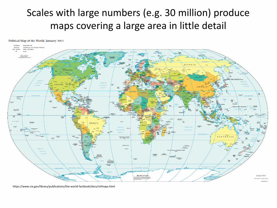
Scales with large numbers (e.g. 30 million) produce maps covering a large area in little detail
https://www.cia.gov/library/publications/the-world-factbook/docs/refmaps.html
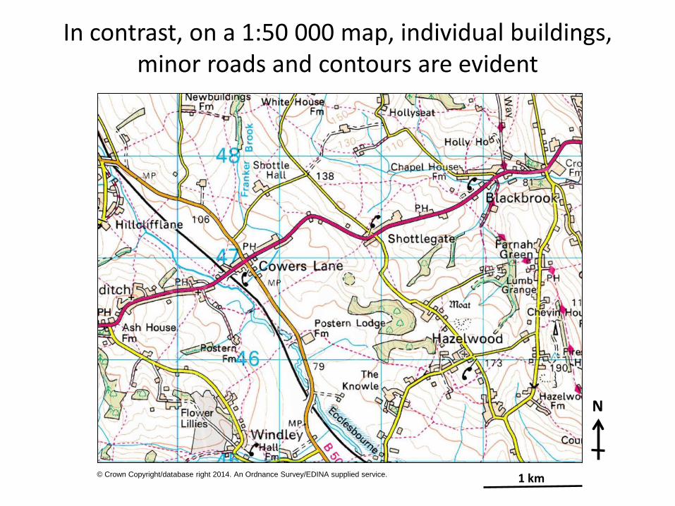
In contrast, on a 1:50 000 map, individual buildings, minor roads and contours are evident
N
© Crown Copyright/database right 2014. An Ordnance Survey/EDINA supplied service. 1 km

200 km
N
The scale bar shows a measurement on the map and the specific distance it represents on the ground
© Crown Copyright/database right 2014. An Ordnance Survey/EDINA supplied service. 1 km
Galway to Dublin is about 200 km
Cowers Lane to Shottlegate is about 1 km
N
Presenter
Presentation Notes
Stress that scale bars are useful when maps are being enlarged or reduced, because they maintain their proportion and can still be used (show reduced inset map as an example)
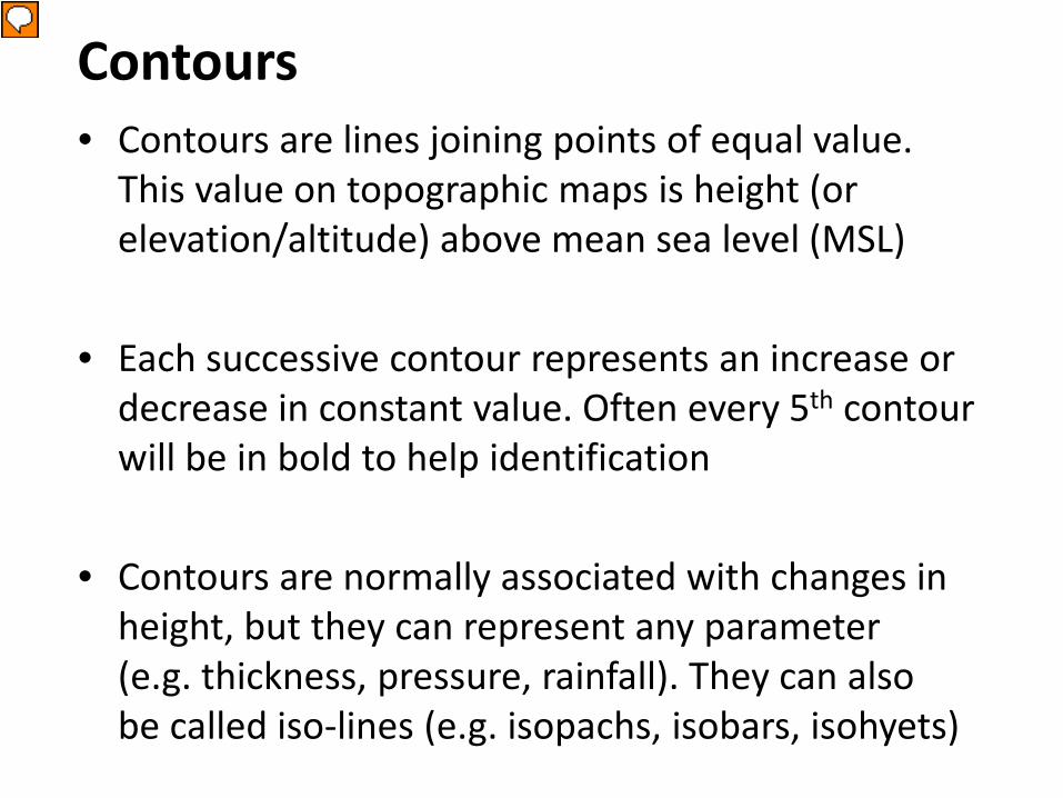
Contours • Contours are lines joining points of equal value.
This value on topographic maps is height (or elevation/altitude) above mean sea level (MSL)
• Each successive contour represents an increase or
decrease in constant value. Often every 5th contour will be in bold to help identification
• Contours are normally associated with changes in
height, but they can represent any parameter (e.g. thickness, pressure, rainfall). They can also be called iso-lines (e.g. isopachs, isobars, isohyets)
Presenter
Presentation Notes
For Ordnance Survey maps the reference point for MSL is taken from Newlyn Harbour, Cornwall.

Contours show the distribution and relative size of any measured value
Surface air pressure is measured in millibars and is shown here as isobars
Presenter
Presentation Notes
What is the contour interval? Answer: 4 millibars Where is the area of highest pressure? Answer: 1037 millibars over Austria Where is the area of lowest pressure? Answer: 979 millibars over the Norwegian Sea

Contours can show the distribution and relative size of any measured value
This map shows the thickness of the Earth’s crust (in kms)
This map shows rainfall data for Australia (in mm)

N
© Crown Copyright/database right 2014. An Ordnance Survey/EDINA supplied service. 1 km
Let’s return to topographic maps - on the map the land surface looks flat, but the contours indicate otherwise
View from Point X towards the SW, showing a valley and
a hill in the distance
X
Presenter
Presentation Notes
Learning to read contours takes practice. You have to visualize the 3-D shape described by the contour patterns.

Contours never cross and will at some point close, although this may be off the map. Topographic contours that close
in concentric patterns delineate hills or depressions
1 km
Presenter
Presentation Notes
Does the diagram show a hill or a depression? Answer: A hill Note that topographic contour values are written with the bottom of the number on the downhill side

Contours are drawn perpendicular to the maximum slope, with the spacing between contours indicating
the steepness of the slope
1 km
Presenter
Presentation Notes
Which direction are the slopes facing? Answer: South How steep is the steep slope? Answer: Not very – it only rises/falls 50m over a kilometre (about 3˚)

Based on the shape of contours, landforms such as valleys and ridges can be recognised
Valley and stream
Ridge
1 km
Presenter
Presentation Notes
Can you recognise a valley and a ridge? Which direction is the stream flowing towards? Answer: South
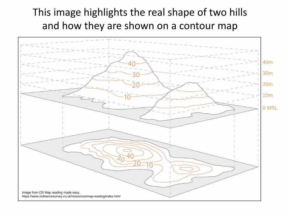
40m 30m 20m 10m 0 MSL
This image highlights the real shape of two hills and how they are shown on a contour map
Image from OS Map reading made easy. https://www.ordnancesurvey.co.uk/resources/map-reading/index.html

You can watch a video explaining how to read contour lines on an Ordnance Survey map
Click here to play…
The Ordnance Survey website has further information on all aspects of maps and map reading, including how to work out grid references and take compass bearings
https://www.ordnancesurvey.co.uk/resources/map-reading/index.html

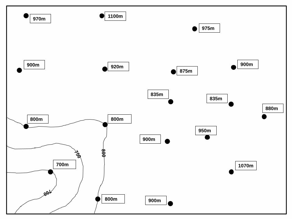
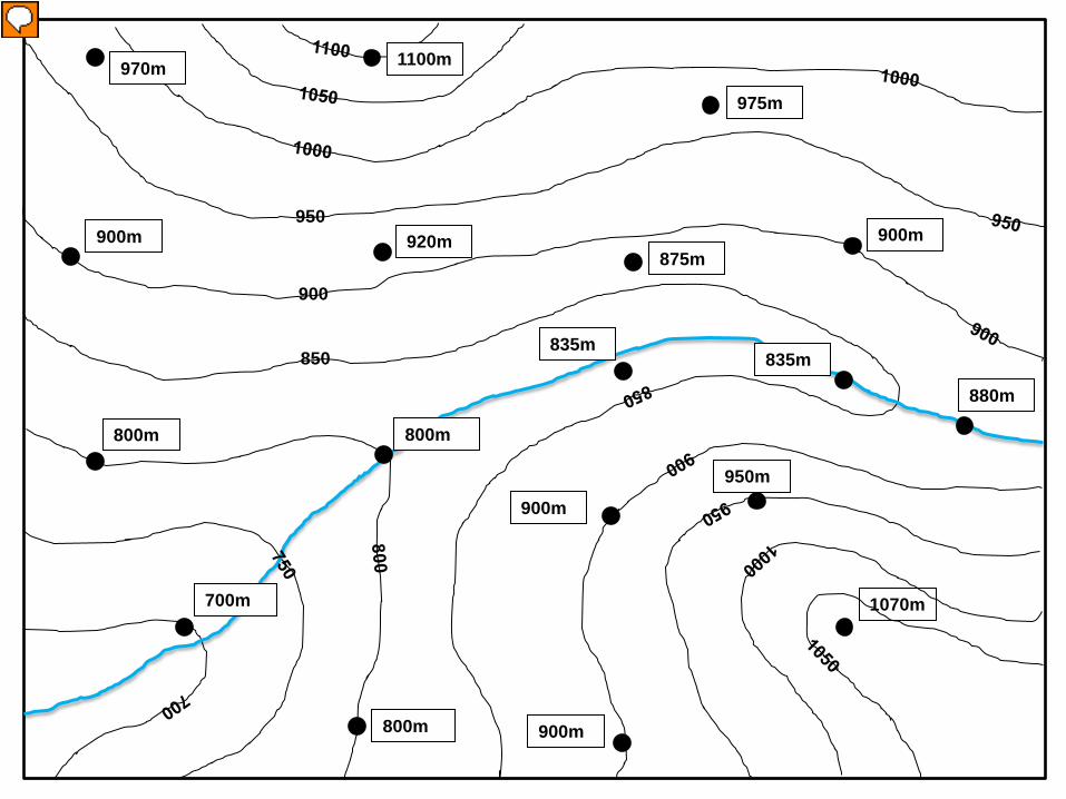
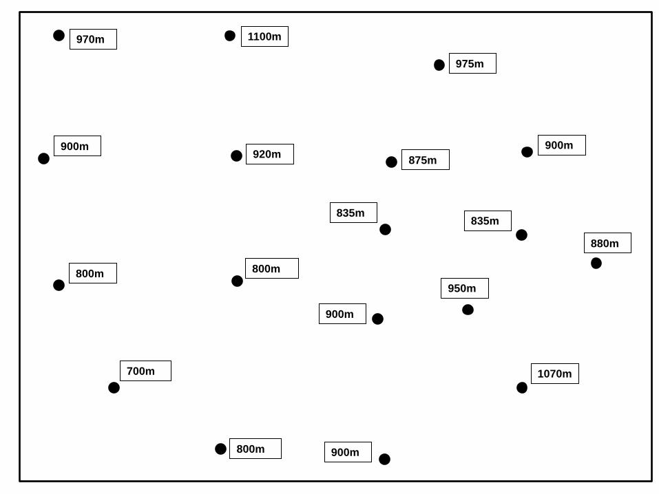
Practical exercise 1 Drawing contours

1100m 970m
975m
900m
900m
900m 920m
800m
800m
1070m
880m
875m
950m
835m 835m
800m
700m
900m
Presenter
Presentation Notes
Sometimes topographic maps are shown with height values at a given point, rather than contours. These are called ‘spot height’ maps and they are rather difficult to interpret. In order to get a better idea of the shape of the land surface the data can be contoured.

800m
800m 700m
800m
700m
900m
750m
800m
850m
Then join up all the original and interpolated points of equal value to form contours.
Start by interpolating between individual points, labelling new values as you go.
750m 750m
750m
The easiest way to draw a contour map based on spot heights is to simply interpolate between the known values. As you interpolate between points make sure you label the new values, as it quickly becomes very confusing if you don’t! Then join identical values with smooth curves to create contours that simulate topography
1100m 970m
975m
900m
900m
900m 920m
800m
800m
1070m
880m
875m
950m
835m 835m
800m
700m
900m

Completing the contouring exercise
• Based on the contour map you have created: • Where is the highest ground? • Where is the lowest area? • Describe the major landforms • Mark on the most likely course of a stream and
determine in which direction it is flowing
Presenter
Presentation Notes
The highest ground is in the north (>1100m). The lowest area is in the SW, in the valley bottom (<700m). The major landforms are a sinuous valley that trends SW-NE, then W-E, flanked by a broad ridge that trends NW-SE. The ground rises from the valley bottom to a high point in the north. The stream is flowing from east to west.
950
900
850
1100m 970m
975m
900m
900m
900m 920m
800m
800m
1070m
880m
875m
950m
835m 835m
800m
700m
900m
Presenter
Presentation Notes
The highest ground is in the north (>1100m). The lowest area is in the SW, in the valley bottom (<700m). The major landforms are a sinuous valley that trends SW-NE, then W-E, flanked by a broad ridge that trends NW-SE. The ground rises from the valley bottom to a high point in the north. The stream is flowing from east to west.
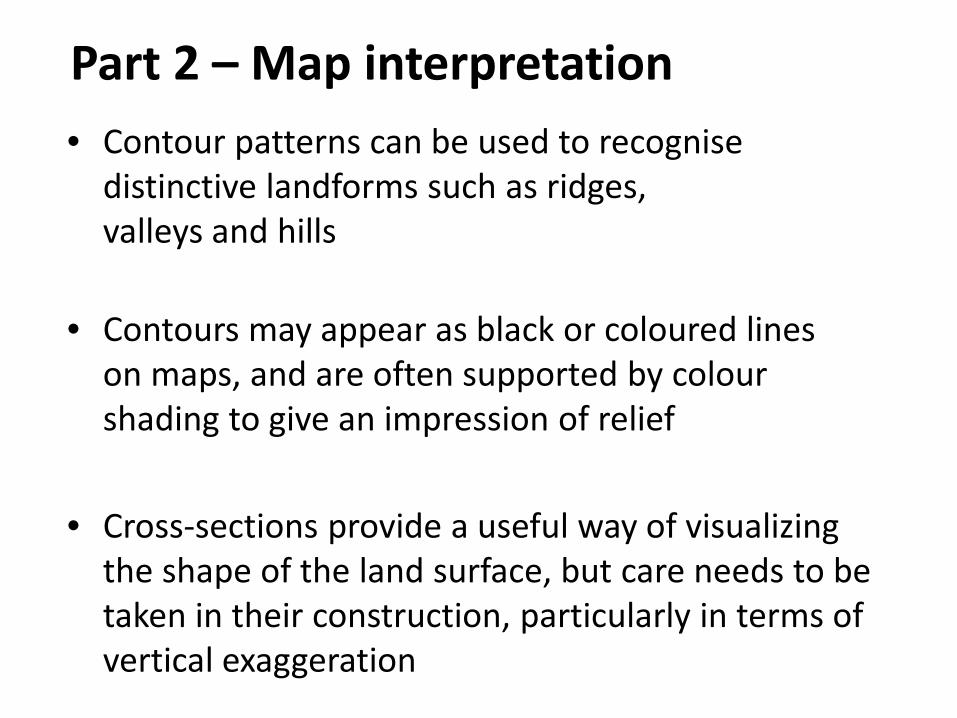
Part 2 – Map interpretation • Contour patterns can be used to recognise
distinctive landforms such as ridges, valleys and hills
• Contours may appear as black or coloured lines on maps, and are often supported by colour shading to give an impression of relief
• Cross-sections provide a useful way of visualizing
the shape of the land surface, but care needs to be taken in their construction, particularly in terms of vertical exaggeration

© Crown Copyright/database right 2014. An Ordnance Survey/EDINA supplied service.
N
1 km
Previously we looked at the topography in this area – let’s take a closer look at the contours

What is the contour interval? Locate the 150m contour between Shottle and Blackbrook
150m contour
© Crown Copyright/database right 2014. An Ordnance Survey/EDINA supplied service.
N
1 km
The contour interval is 10m with bold lines every 50m

If you walked along this contour, what would your route be like? Flat, as long as you remain on the 150m contour
150m contour
© Crown Copyright/database right 2014. An Ordnance Survey/EDINA supplied service.
N
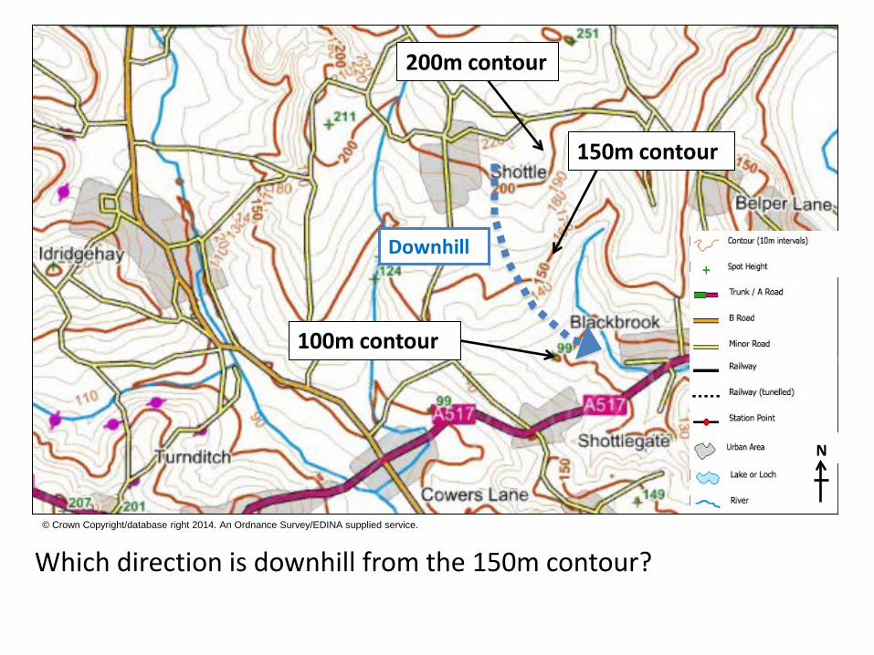
Which direction is downhill from the 150m contour?
150m contour
© Crown Copyright/database right 2014. An Ordnance Survey/EDINA supplied service.
N
200m contour
100m contour
Downhill

What else about the contours help to determine the direction of slope?
© Crown Copyright/database right 2014. An Ordnance Survey/EDINA supplied service.
N
The contour values are perpendicular to the slope, with the bottom of the number on the downhill side

What does the hillside look like if you stand at Point A and look towards Point B?
B A
© Crown Copyright/database right 2014. An Ordnance Survey/EDINA supplied service.
N
1 km
It would go downhill to the stream and then uphill again to Point B
100 200 300 400 500 600 700 800 900
100
200
A B
Con
tour
val
ue (m
etre
s)
Distance (metres)
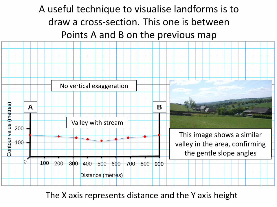
Valley with stream
0
No vertical exaggeration
This image shows a similar valley in the area, confirming
the gentle slope angles
A useful technique to visualise landforms is to draw a cross-section. This one is between
Points A and B on the previous map
The X axis represents distance and the Y axis height
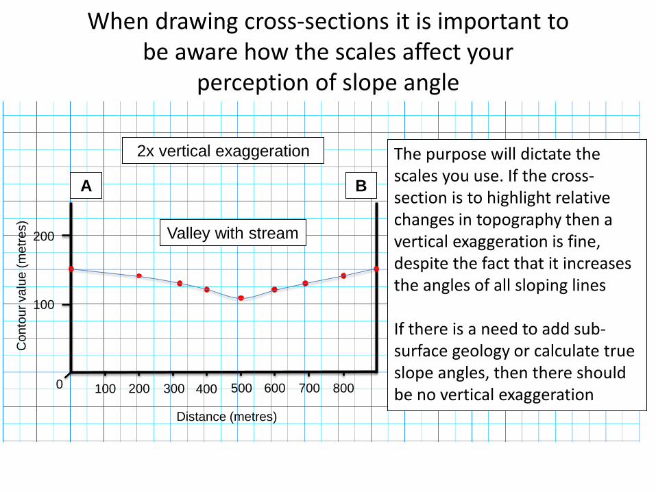
100 200 300 400 500 600 700 800
100
200
A B
Con
tour
val
ue (m
etre
s)
Distance (metres)
Valley with stream
0
2x vertical exaggeration
When drawing cross-sections it is important to be aware how the scales affect your
perception of slope angle
The purpose will dictate the scales you use. If the cross- section is to highlight relative changes in topography then a vertical exaggeration is fine, despite the fact that it increases the angles of all sloping lines If there is a need to add sub-surface geology or calculate true slope angles, then there should be no vertical exaggeration

Notice how the change in vertical exaggeration affects the angles of slope Bear this in mind when drawing your own cross-sections and decide how much (if any) vertical exaggeration is required
Compare the effects of vertical exaggeration on the same cross-section

You now know how to identify a sloping valley by the shape of the contours.
© Crown Copyright/database right 2014. An Ordnance Survey/EDINA supplied service.
N
Uphill
They form a V-shape that points uphill

There are lots of valleys on the map; mark them with an arrow pointing in the downhill direction
Arrows indicate downhill direction of valleys
© Crown Copyright/database right 2014. An Ordnance Survey/EDINA supplied service.
N
Presenter
Presentation Notes
This map shows some of the main valleys (not all have been marked)

Notice that all the rivers are in valleys, but not all the valleys have a river. Why is this the case?
© Crown Copyright/database right 2014. An Ordnance Survey/EDINA supplied service.
N
Arrows indicate downhill direction of valleys
Presenter
Presentation Notes
There is no permanent water in these valleys, however in the past there was sufficient water that flowed along these routes to cause erosion and form the valley. Is there any time in the recent geological past when there was greater water flow in this area?
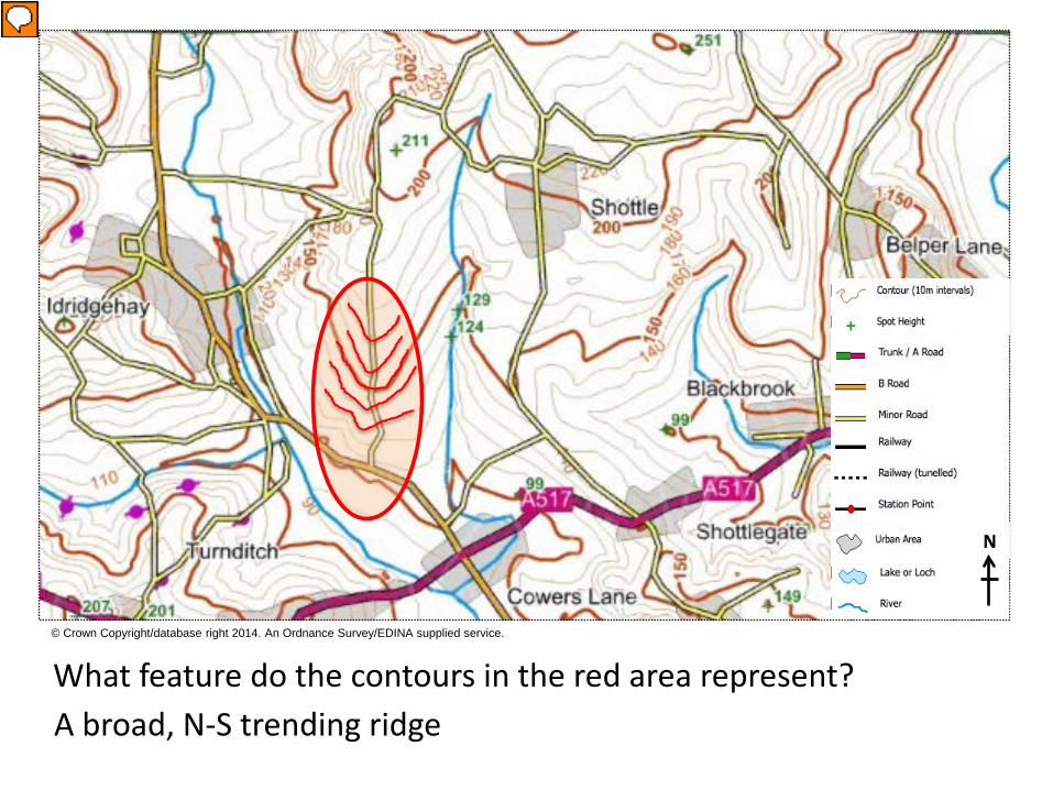
What feature do the contours in the red area represent? © Crown Copyright/database right 2014. An Ordnance Survey/EDINA supplied service.
N
A broad, N-S trending ridge
Presenter
Presentation Notes
Notice that the contours have a similar shape to a valley, but the V-shape points downhill

It may help if you imagine you are standing at Point C on the 150m contour, looking towards Point D. Would you be able to see Point D?
We can draw a cross-section to confirm our idea
© Crown Copyright/database right 2014. An Ordnance Survey/EDINA supplied service.
N
C D
Axis of ridge
Presenter
Presentation Notes
Answer: No; Point D is at the same height (150m) as Point C, but the axis of the ridge is higher (at 175m).
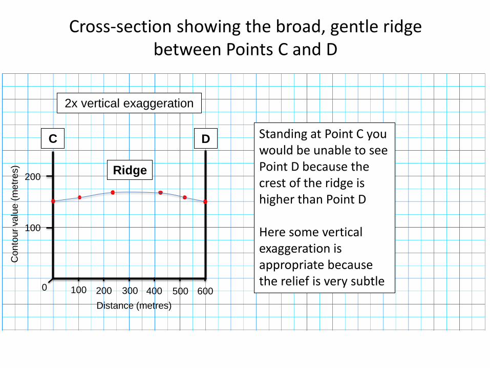
100 200 300 400 500 600
100
200
C D
Con
tour
val
ue (m
etre
s)
Distance (metres)
Ridge
Cross-section showing the broad, gentle ridge between Points C and D
0
2x vertical exaggeration
Standing at Point C you would be unable to see Point D because the crest of the ridge is higher than Point D Here some vertical exaggeration is appropriate because the relief is very subtle
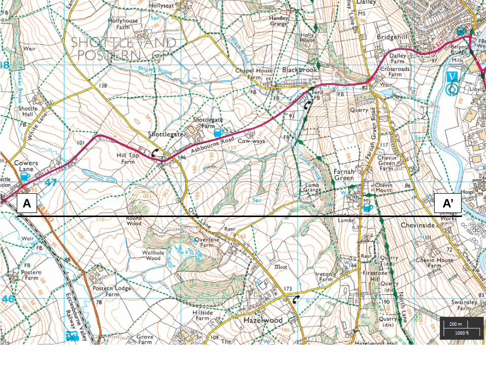
Practical exercise 2 Constructing cross-sections

A A’
Before constructing a cross-section, look at the contours and try to imagine what the surface topography looks like
Closely spaced contours showing a steep slope
Widely spaced contours showing less steep slopes compared to those in the east
Narrower range of contours between 140-160m indicate a relatively flat hill top
We will now draw our own cross-section between Cowers Lane (A) and Chevinside (A’)

A A’
Use graph paper to mark on every time a contour crosses the chosen line of section
85
90
95
100 105 110
150m
200m
100m
50m
Label each contour height and plot the value directly onto the Y-axis of the cross-section

A A’
Once all the contour heights along the section have been plotted the land surface can be added
50m
100m
150m
200m
This surface should be drawn free hand to give a natural shape that honours the contours
4x vertical exaggeration

150m
100m
50m
0
200m A A’
1 km 2 km 3 km
A completed cross-section between A-A’ The vertical scale has been exaggerated in order to show the subtle relief. To calculate the vertical exaggeration, divide the horizontal scale (1cm to 200m) by the vertical scale (1cm to 50m) So, 200/50 = 4x vertical exaggeration
West East
Scale 1: 20 000
4x vertical exaggeration
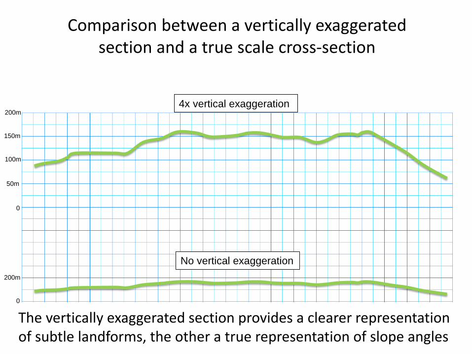
Comparison between a vertically exaggerated section and a true scale cross-section
200m
0
No vertical exaggeration
100m
150m
50m
200m
0
4x vertical exaggeration
The vertically exaggerated section provides a clearer representation of subtle landforms, the other a true representation of slope angles
You have now been introduced to the basic elements of topographic maps You have used contours to identify common landforms and begun to visualise them in 3-D You can now construct cross-sections and understand the concept of vertical exaggeration
Learning outcomes

Slide 50: print out at A4, in B/W, portrait format Slide 51: print out at A4, in colour, portrait format Slide 52: print out at A4, in colour, portrait format Graph paper for constructing the cross-section
Handouts required for the practicals
1100m 970m
975m
900m
900m
900m 920m
800m
800m
1070m
880m
875m
950m
835m 835m
800m
700m
900m

© Crown Copyright/database right 2014. An Ordnance Survey/EDINA supplied service.
N
1 km
A A’