AN INFORMATION ELASTICITY FRAMEWORK FOR CONSTANT …
115
The Pennsylvania State University The Graduate School AN INFORMATION ELASTICITY FRAMEWORK FOR CONSTANT FALSE ALARM RATE DETECTION A Thesis in Electrical Engineering by Andrew Z. Liu © 2020 Andrew Z. Liu Submitted in Partial Fulfillment of the Requirements for the Degree of Master of Science May 2020
Transcript of AN INFORMATION ELASTICITY FRAMEWORK FOR CONSTANT …
The Pennsylvania State University
The Graduate School
AN INFORMATION ELASTICITY FRAMEWORK FOR
CONSTANT FALSE ALARM RATE DETECTION
A Thesis inElectrical Engineering
byAndrew Z. Liu
© 2020 Andrew Z. Liu
Submitted in Partial Fulfillmentof the Requirements
for the Degree of
Master of Science
May 2020

The thesis of Andrew Z. Liu was reviewed and approved by the following:
Ram M. NarayananProfessor of Electrical EngineeringThesis Adviser
Timothy J. KaneProfessor of Electrical Engineering
Muralidhar RangaswamySpecial Member
Kultegin AydinProfessor of Electrical EngineeringHead of the Department of Electrical Engineering
ii

Abstract
Within a decision making process, adjusting the amount of available information generally
causes the effectiveness of decisions to change. Often, an increase in this information quantity
causes the decision effectiveness to improve. However, under certain circumstances, increas-
ing the amount of information beyond a certain point causes the decision effectiveness to
suffer. This phenomenon, known as information overload, presents many important research
problems. One major concern is determining how much information a decision maker needs
for the decision effectiveness to be maximized. Another key problem is defining the metrics
that are used to model information quantity and decision effectiveness, given the specific
contextual factors and preferences of a decision maker. Recently, the concept of information
elasticity has been proposed to address these problems.
This thesis aims to design a framework using the concept of information elasticity to
observe the usability of information within different constant false alarm rate detectors.
Within this framework, the different factors which either benefit or hinder the performance
of these detectors are studied, and are used along with contextual factors to characterize the
effectiveness of decisions. Within this thesis, two different applications of this framework are
studied. The first involves the ordered statistics constant false alarm rate detector, and the
second involves the adaptive matched filter. The point at which information overload occurs
is uncovered within each of these applications, allowing a decision maker to make choices
that maximize the decision effectiveness.
iii

Contents
List of Figures vii
List of Tables xi
Dedication xii
Acknowledgments xiii
1 Introduction 1
1.1 Introduction to Information Elasticity . . . . . . . . . . . . . . . . . . . . . . 1
1.2 Introduction to CFAR detection . . . . . . . . . . . . . . . . . . . . . . . . . 3
2 Background Theory 5
2.1 Information Elasticity . . . . . . . . . . . . . . . . . . . . . . . . . . . . . . 5
2.1.1 General Framework . . . . . . . . . . . . . . . . . . . . . . . . . . . . 5
2.1.2 Application of Information Elasticity: Phase coded modulation . . . . 7
2.2 Topics in Multi-Objective Optimization . . . . . . . . . . . . . . . . . . . . . 11
3 Fundamentals of CFAR Detection 14
3.1 Detection Theory . . . . . . . . . . . . . . . . . . . . . . . . . . . . . . . . . 14
3.1.1 Coherent Detection . . . . . . . . . . . . . . . . . . . . . . . . . . . . 14
3.1.2 Range Resolution . . . . . . . . . . . . . . . . . . . . . . . . . . . . . 16
3.1.3 Performance measures for detection . . . . . . . . . . . . . . . . . . . 17
iv

3.1.4 Statistical analysis of interference and targets . . . . . . . . . . . . . 18
3.2 Scalar CFAR detection . . . . . . . . . . . . . . . . . . . . . . . . . . . . . . 22
3.2.1 Likelihood Ratio Test . . . . . . . . . . . . . . . . . . . . . . . . . . . 22
3.2.2 Distribution of Test Statistic . . . . . . . . . . . . . . . . . . . . . . . 24
3.2.3 PFA and PD of detector . . . . . . . . . . . . . . . . . . . . . . . . . 28
3.2.4 Performance under Swerling Fluctuation Models . . . . . . . . . . . . 30
4 Robust Decision Making for Ordered Statistic CFAR 35
4.1 Ordered Statistic CFAR . . . . . . . . . . . . . . . . . . . . . . . . . . . . . 35
4.1.1 OS-CFAR performance . . . . . . . . . . . . . . . . . . . . . . . . . . 36
4.1.2 Effects of Interfering targets . . . . . . . . . . . . . . . . . . . . . . . 42
4.2 Information Elasticity Framework for OS-CFAR . . . . . . . . . . . . . . . . 45
4.2.1 Estimation of J using FAOSOSD . . . . . . . . . . . . . . . . . . . . 46
4.2.2 Performance Function for OS-CFAR . . . . . . . . . . . . . . . . . . 49
4.2.3 Robust decision making method . . . . . . . . . . . . . . . . . . . . . 50
5 Information Elasticity Framework for the AMF 53
5.1 Clairvoyant Detector . . . . . . . . . . . . . . . . . . . . . . . . . . . . . . . 54
5.1.1 Likelihood Ratio Test . . . . . . . . . . . . . . . . . . . . . . . . . . . 54
5.1.2 PD and PFA of Clairvoyant Detector . . . . . . . . . . . . . . . . . . 56
5.2 Adaptive Matched Filter . . . . . . . . . . . . . . . . . . . . . . . . . . . . . 59
5.2.1 Sample Matrix Inversion . . . . . . . . . . . . . . . . . . . . . . . . . 60
5.2.2 Rank Constrained Maximum Likelihood Estimation . . . . . . . . . . 64
5.2.3 Additional SNR required for clairvoyant performance . . . . . . . . . 68
5.3 Information Elasticity Framework for the AMF . . . . . . . . . . . . . . . . 71
5.3.1 Approximation for SNR loss . . . . . . . . . . . . . . . . . . . . . . . 73
5.3.2 User-defined constraint function . . . . . . . . . . . . . . . . . . . . . 79
5.3.3 AMF decision effectiveness . . . . . . . . . . . . . . . . . . . . . . . . 80
v

6 Conclusion 89
APPENDICES 90
Derivation of the AMF 91
A.0.1 Distribution of AMF test statistic . . . . . . . . . . . . . . . . . . . . 95
vi

List of Figures
1 Decision effectiveness shown as a function of information quantity, displaying
an example of the inverted U-curve. . . . . . . . . . . . . . . . . . . . . . . . 3
2 Output of matched filter using PCM pulse compression, shown using two
waveforms with frequency f = 5MHz. The waveform compressed in (a) has a
signal length of T = 1.5 µs, code length of 15 bits, and chip length TC = 0.1 µs.
The waveform compressed in (a) has a length of T = 3.1 µs, code length of
31 bits, and chip length TC = 0.1 µs. . . . . . . . . . . . . . . . . . . . . . . 9
3 D(Q) (PSLR) shown as a function of Q (sequence length). . . . . . . . . . . 10
4 C(Q) (autocorrelation computation time) shown as a function of Q. . . . . . 10
5 E(Q) (PSLR per ns of processing time) shown as a function of Q (sequence
length). . . . . . . . . . . . . . . . . . . . . . . . . . . . . . . . . . . . . . . 10
6 Example showing decisions in the criterion space along with their Pareto fron-
tier, utopia point, and nadir point. . . . . . . . . . . . . . . . . . . . . . . . 12
7 distributions . . . . . . . . . . . . . . . . . . . . . . . . . . . . . . . . . . . . 20
8 distributions . . . . . . . . . . . . . . . . . . . . . . . . . . . . . . . . . . . . 21
11 Probability distributions for the sufficient statistic Λ under hypotheses 0 and
1. The H1 distributions are shown for 3 different SNR values. . . . . . . . . 26
12 PD as a function of SNR (SNR is represented with A in equation (38)) for
different values of K for PFA = 1 · 10−6. . . . . . . . . . . . . . . . . . . . . . 31
vii

13 PD vs SNR curves shown for the Swerling I, Swerling III, and non-fluctuating
case for K = 10 and PFA = 10−4. Note that the PD vs SNR curves for
Swerling II and Swerling IV are equal to that of Swerling I and Swerling III
respectively when scalar data samples are used. . . . . . . . . . . . . . . . . 34
14 PD vs m for K = 24 and PFA = 1 · 10−4, shown for different SNR values. . . 41
15 PD vs SNR for K = 24 and PFA = 1 · 10−4 for the Swerling I case, shown for
both CA-CFAR. . . . . . . . . . . . . . . . . . . . . . . . . . . . . . . . . . . 41
16 Effects of interfering targets on PD vs m shown at RSS = 10 dB. Note that
the results from 106 Monte Carlo simulations is displayed with the dotted
curves, showing close agreement with the results in (61). α is found via (53)
for PFA = 10−4. . . . . . . . . . . . . . . . . . . . . . . . . . . . . . . . . . . 44
17 Effects of interfering targets on PD vs m shown at RSS = 20 dB. Note that
the results from 106 Monte Carlo simulations is displayed with the dotted
curves, showing close agreement with the results in (61). α is found via (53)
for PFA = 10−4. . . . . . . . . . . . . . . . . . . . . . . . . . . . . . . . . . . 45
18 Effects of interfering targets on PFA vs m for RSS = 10 dB. α is found via
(53) for PFA = 10−4. . . . . . . . . . . . . . . . . . . . . . . . . . . . . . . . 46
19 P (J |J) shown for K = 20 and different RSS values. . . . . . . . . . . . . . . 48
20 ψ0 shown for P ∗FA = 1 · 10−4. . . . . . . . . . . . . . . . . . . . . . . . . . . . 49
21 µ(x,A) vs Var(x,A) shown for J = 5, N = 20, and P ∗FA = 10−4. Points
shown for 8400 decision points and A = {5, 10, . . . , 90, 95}. Pareto frontier is
shown by the black curve. . . . . . . . . . . . . . . . . . . . . . . . . . . . . 51
22 Decision effectiveness shown as a function of the measure of robustness, Var.
Note that the overload point occurs at the decision m = 12 and α = 8.8940. . 52
23 PD vs SNR for PFA = 1 · 10−4 and N = 10 shown for different values of K. . 63
24 PD vs SNR for PFA = 1 · 10−4 and N = 30 shown for different values of K. . 63
viii

25 PD vs SNR for PFA = 1 · 10−4 and N = 20 shown for different values of K.
Note that the degenerate N = K case is shown in blue. . . . . . . . . . . . . 64
26 PD vs SNR curves shown forN = 16, r = 7, K = {3, 4, . . . , 24}, and PFA = 10−4. 67
27 PD vs SNR curves shown for N = 24,r = 9, K = {3, 4, . . . , 24}, and PFA = 10−4. 68
28 PD vs SNR for PFA = 10−4 and K = {N, . . . , 200}, shown for different N
values. Note that darker curves represent PD values of larger K values. . . . 69
29 SNR loss for AMFs of different N values, shown as a function of K. . . . . . 70
30 SNR loss for RCML AMFs of different N and r values, shown as a function
of K. . . . . . . . . . . . . . . . . . . . . . . . . . . . . . . . . . . . . . . . . 70
31 Comparison of PD obtained using numerical methods as in (97) and approxi-
mation as in (101). PD is shown for N = 5, PFA = {10−4, 10−5, 10−6} values
and K = {5, 10, . . . , 50}. . . . . . . . . . . . . . . . . . . . . . . . . . . . . . 76
32 Comparison of PD obtained using numerical methods as in (97) and approxi-
mation as in (101). PD is shown for N = 50, PFA = {10−4, 10−5, 10−6} values
and K = {50, 51, . . . , 100}. . . . . . . . . . . . . . . . . . . . . . . . . . . . 77
33 Comparison of PD obtained using numerical methods as in (97) and approxi-
mation as in (101). PD is shown for N = 500, PFA = {10−4, 10−5, 10−6} values
and K = {500, 510, . . . , 600}. . . . . . . . . . . . . . . . . . . . . . . . . . . 78
34 SNR loss as a function K. Calculations from numerical methods in (97) and
approximation in (102) are displayed together, showing close agreement. . . . 79
35 Constraint function C1(Q) for λ1 = λ2 = 0.5, n = m = 1, a = 10−4, b = 10−6,
c = 40, and d = 60. . . . . . . . . . . . . . . . . . . . . . . . . . . . . . . . . 81
36 Constraint function C2(Q) for λ1 = 1/3, λ2 = 2/3, n = 2,m = 4, a = 10−4,
b = 10−6, c = 40, and d = 60. . . . . . . . . . . . . . . . . . . . . . . . . . . 81
37 Decision metric D(Q) for the AMF using SMI and N = 20. Domain param-
eters are a = 10−4, b = 10−6, c = 40. Note that the PFA and K axes are
inverted from the axes in Figures 35 and 36. . . . . . . . . . . . . . . . . . . 82
ix
38 C1(Q) and D(Q) for different decision points for N = 20. Note that points
of a shared color represent data of a shared K value. . . . . . . . . . . . . . 83
39 C2(Q) and D(Q) for different decision points for N = 20. Note that points
of a shared color represent data of a shared K value. . . . . . . . . . . . . . 83
40 Pareto fronts for C1(Q) and D(Q), as well as C2(Q) and D(Q). Note that
these are labeled as Pareto front #1 and Pareto front #2 respectively. . . . . 84
41 Decision effectiveness E of Pareto efficient decisions shown as a function of
their cost C1(Q). . . . . . . . . . . . . . . . . . . . . . . . . . . . . . . . . . 85
42 Decision effectiveness E of Pareto efficient decisions shown as a function of
their cost C2(Q). . . . . . . . . . . . . . . . . . . . . . . . . . . . . . . . . . 86
x

List of Tables
1 Threshold value α for different values of m and K and for PFA = 1 · 10−4.
These values are obtained using a MATLAB routine involving a line search
method on equation (53). . . . . . . . . . . . . . . . . . . . . . . . . . . . . . 40
2 Decisions at which E is minimized for DM 1. . . . . . . . . . . . . . . . . . 85
3 Decisions at which E is minimized for DM 2. . . . . . . . . . . . . . . . . . 85
4 Constraint function parameters. . . . . . . . . . . . . . . . . . . . . . . . . . 87
5 Specification for decision metrics. . . . . . . . . . . . . . . . . . . . . . . . . 87
6 Decisions at which E is minimized for different constraint functions and deci-
sion metrics. Note that w1 = w2 for each decision. . . . . . . . . . . . . . . . 88
xi

Dedication
This thesis is dedicated to my parents, Zheji and Xia, siblings, Michael and Sarah, and wife,
Kristi. Their love and encouragement gave me the inspiration to begin and complete this
academic journey. Also, to God, who upholds me each day.
‘His faithfulness is a shield and bulwark.’ (Psalm 91:4b)
xii

Acknowledgments
The completion of this thesis would not have been possible without the support of my thesis
advisor, Dr. Ram Narayanan. I am extremely grateful for his patience, understanding,
encouragement, and advice which has profoundly impacted me for the better. I would also
like to express gratitude to Dr. Muralidhar Rangaswamy. I am deeply thankful for his
invaluable guidance and expertise, and for his help in establishing foundational concepts in
this work. I would also like to thank Dr. Timothy Kane for serving on my thesis committee,
and for generously offering his time and support. Thanks should also go to the members
of the Radar and Communications Lab for their insight into different topics covered in this
research.
Finally, I would like to extend thanks to Dr. Doug Riecken of the US Air Force Office of
Scientific Research for supporting this research under grant FA9550-17-1-0032.
This content is the solely the responsibility of the author, and does not necessarily rep-
resent the views of the funding agency.
xiii

Chapter 1
Introduction
1.1 Introduction to Information Elasticity
The task of radar detection often requires the selection of different decision parameters,
which are chosen with the goal of improving the overall performance of the system. This
choice of parameters and the definition of “performance” generally vary between contexts
and the decision makers (DM) making choices within them. For example, a decision may
be selected in such a way that produces poor performance for one DM in a given context,
that may also produce good performance for a DM in another context. Thus, the contextual
factors and preferences of the DM must be carefully characterized in order for decisions to
be compared and analyzed.
Information elasticity is a concept that has recently been proposed [1] which seeks to char-
acterize the usability properties of information and its interaction its surrounding context.
Note that in this sense, information does not specifically refer to the concept of Shannon’s
entropy or other concepts in information theory. Rather, it refers to information in a general
sense: information takes the form of data, signals, or processes which increases the knowledge
level of a DM.
With this in mind, certain decision parameters have the ability to affect the quantity of
1

2
information seen by a radar system. When these parameters are adjusted, the quantity of
information and the general effectiveness of these decision parameters change. It is generally
assumed that the effectiveness of decisions improves as the quantity of information increases.
However, it has been shown that this is not always the case, and in certain instances, more
information may actually cause the decision effectiveness to worsen [2],[3],[4].
Information elasticity is defined as the ratio of incremental change in decision effectiveness
and the incremental change in the quantity of information [5]. Thus, a system characterized
by a high information elasticity sees a large increase in decision effectiveness as more infor-
mation is available. Similarly, a system with low information elasticity sees a small increase
in decision effectiveness as more information is available. Furthermore, a system with a
negative information elasticity sees a decrease in decision effectiveness as more information
is available.
Since these measures of information quantity and decision effectiveness generally depend
on contextual factors, they must be specified by a DM. The decision effectiveness, as defined
by a DM, is often affected by two types of factors. The first type are known as decision
quality metrics, which generally take the form of attributes that aid a DM in making better
decisions. For radar applications, examples of decision quality metrics may be probability of
detection or signal-to-noise ratio (SNR). The second type are known as constraint metrics,
which generally take the form of attributes that are undesirable in high levels. Examples of
radar constraint metrics may be processing time or power usage.
These metrics are generally functions of the information quantity, and in many cases
exhibit conflicting trade-off behavior. Typically, as the information quantity increases, the
decision quality metrics see improvement. On the other hand, this increase in information
quantity is also associated with an increase in the undesirable constraints. Under certain
circumstances, increasing the information quantity beyond a certain point may cause the
effects from the system constraints to dominate the effects from the decision quality metrics,
resulting in a decrease in decision effectiveness (information elasticity is negative). When

3
Figure 1: Decision effectiveness shown as a function of information quantity, displaying anexample of the inverted U-curve.
a system reaches this point, the decision effectiveness reaches a maximum, and increasing
the information quantity no longer provides any benefit. This phenomenon is known as
information overload and is shown in the form of an example in Figure 1. The exact point at
which information overload occurs is of interest, since it allows the decision maker to select
the decision that maximizes the decision effectiveness.
1.2 Introduction to CFAR detection
The detection of targets in the presence of clutter, noise, and other disturbances is an
important signal processing problem for many different radar systems. Typically a “detection
threshold” is defined, which is used to declare data values above the threshold as targets and
data values below the threshold as merely disturbance. Certain assumptions can often be
made involving the statistical behavior of this disturbance, allowing for different detection
schemes to be used. Since radar disturbance and interference generally vary depending on
the time/range at which the data are collected (non-stationary disturbance), these detection
schemes are often adaptive, and change according to the disturbance surrounding the data
under test.
Many commonly used adaptive schemes change the detection threshold to fix the rate
at which data containing disturbance only is mistakenly declared as a target (also known

4
as a false alarm). Any detector that accomplishes this task is known to have the constant
false alarm rate (CFAR) property. With this property, a detector is able to achieve a desired
performance level in the receiver operating characteristic space (discussed in Chapter 3.1).
Often, radar data are obtained as a collection of scalar values, representing the power
received from different range bins. This data is used to form decision statistics for each
range bin, which are thereby compared against the detection threshold. Different detection
algorithms typically use different types of decision statistics, depending on the application
of the radar system and the types of limitations they wish to overcome. Two commonly
used algorithms, which are analyzed in this thesis, are cell-averaging CFAR (CA-CFAR)
and ordered statistics CFAR (OS-CFAR) [6].
Other radar systems collect range data over a multitude of different antenna elements as
well as across different pulses sent by each element. In this case, each range bin is represented
by a 1 ×N vector rather than a singular scalar value. This parameter, N , is known as the
spatio-temporal product [7], and is simply the number of antenna elements of the radar
system multiplied with the number of pulses being considered. This thesis studies a well
known multi-dimensional CFAR detector known as the adaptive matched filter (AMF)[8].
The goal of this thesis is to analyze where this information overload behavior exists in
different applications of CFAR detection, and exploit it to make decisions with maximum
decision effectiveness. To accomplish this task, an information elasticity framework is em-
ployed in two different applications using CFAR detection, the first application involving
OS-CFAR, and the second involving the AMF. This thesis is organized as follows: Chapter
2 provides an overview on information elasticity and topics in multi-objective optimization.
Chapter 3 reviews background detection theory as well as analyzes the scalar CA-CFAR
detector. Chapter 4 analyzes the performance of the OS-CFAR detector, and presents an in-
formation elasticity framework which seeks to increase the robustness of decisions. Chapter
5 analyzes the performance of the AMF, and presents an information elasticity framework
for making decisions within different contexts. Chapter 6 serves as the conclusion.

Chapter 2
Background Theory
2.1 Information Elasticity
2.1.1 General Framework
As discussed in Section 1.1, information elasticity is defined as the ratio of the incremen-
tal change of decision effectiveness with respect to the incremental change of information
quantity. This is denoted as follows [5]:
ε =dE/E
dQ/Q(1)
where ε is the information elasticity, E is the decision effectiveness, and Q is the information
quantity. Thus, dQ represents the infinitesimal variation in information quantity, and dE
represents its associated infinitesimal variation in decision effectiveness. Note that it is
possible for Q to be defined such that it exists only in discrete quantities. In this case, these
differential terms are replaced by their respective forward difference terms, ∆E and ∆Q.
The decision effectiveness is generally a function of the decision quality and constraint
metrics described in Section 1.1. Furthermore, each of these metrics are functions of the
information quantity Q. The decision quality metric, represented by D(Q), is defined such
5

6
that it improves as Q increases. Similarly, the constraint function C(Q) is defined such that
it gets worse as Q increases. Thus, both D(Q) and C(Q) are monotonic in Q. Whether
these functions monotonically increase or decrease depends on whether it is desirable for
D(Q) or C(Q) to be minimized or maximized. From these definitions, a trade-off behavior
exists between D(Q) and C(Q), since increasing Q causes a better decision metric, but a
worse constraint function.
Note that the form of E is dependent on the DM. Consider the following simple model
for decision effectiveness:
E =D(Q)
C(Q)(2)
This formulation for decision effectiveness can be thought of as representing the amount of
decision quality achieved per unit of constraint metric. Note that in subsequent chapters,
other formulations for E are used.
Using this simple formulation, the elasticity ε can be broken down as follows. From (2):
ln(E(Q)) = ln(D(Q))− ln(C(Q))
Differentiating with respect to Q yields:
1
E
dE
dQ=
1
D
dD
dQ− 1
C
dC
dQ
=⇒ dE/E
dQ/Q=
dD/D
dQ/Q− dC/C
dQ/Q
The partial elasticities of D and C are defined as:
εD =dD/D
dQ/Q(3)
εC =dC/C
dQ/Q(4)

7
Thus, the elasticity ε can be decomposed as:
ε = εD − εC (5)
At the point of information overload, ε = 0. Thus, in order for information overload to occur
for this particular formulation for E, there must be some value of Q such that εD = εC .
Consider also that it is possible for a decision maker to use multiple decision quality
metrics and constraint metrics [2], which are represented as Ck(Q), k = 1, 2, . . . , K and
Cl(Q), l = 1, 2, . . . , L respectively. A simple example for a decision effectiveness that uses
multiple decision quality and constraint metrics is given as follows:
E =
∏Kk=1D
mkk∏L
l=1Cnll
(6)
where mk and nl represent exponential weightings, which allow a DM to specify emphasis
on metrics that have greater importance. Using the same rearrangements used above, the
elasticity of this particular model can be broken down as:
ε =K∑k=1
mkεDk +L∑l=1
mlεDl (7)
2.1.2 Application of Information Elasticity: Phase coded modu-
lation
In this section, the decision effectiveness model in (2) is used on an example radar application
to demonstrate how the information elasticity framework can be used to make decisions.
This example specifically deals with the application of using phase-coded modulated (PCM)
waveforms for the purpose of pulse compression. This technique is used by many radar
systems to improve the resolution and SNR of a radar. Pulse compression is implemented
using a matched filter, which considers the auto-correlation of a signal. Auto-correlation can

8
be thought of as the cross correlation of a signal with a time-reversed copy of itself [9].
Consider the cross-correlation operation defined as follows:
rxy[m] =∞∑
n=−∞
x[n]y[m− n] (8)
where x[n] is a copy of the transmitted waveform and y[n] is the received waveform. Let us
assume that the radar waveform is typically modulated in a way such that when matched
filtering occurs, the majority of the energy is compressed into a single main pulse of decreased
width. In particular, PCM separates the waveform into sections of equal length known as
chips. A phase shift is applied to each chip based on a given code, or sequence of numbers.
While many different types of codes exist, binary sequences are often considered due
to their simplicity and ease of implementation. In particular, maximal-length sequences
(MLSs) are a class of binary sequences that exhibit desirable auto-correlation properties
[10]. These codes are generated using linear feedback shift registers with taps located at
specific locations. These shift registers produce cyclic sequences, with periods of 2n− 1 bits,
where n is the number of stages in the shift register. Thus, MLS’s only exist in lengths of
2n − 1.
Two examples of pulse compression using PCM are shown in Figure 2. These examples
show that after modulating the waveforms, most of the energy of the signal is now concen-
trated in the central lobe, also known as the mainlobe. Note also, however, that some of the
energy exists outside of the main lobe, in sections of the signal known as sidelobes. These
sidelobes are often problematic in ranging radar applications, since sidelobes associated with
a strong target may mask the main lobe of a weaker target, preventing a user from detecting
the presence of the weaker target [9]. Thus, the metric known as peak-sidelobe ratio (PSLR)
is often used to characterize the size of the sidelobe relative to the main lobe. Generally,
this metric is simply the ratio between the magnitude of the mainlobe to the magnitude of
the largest sidelobe. Clearly, a larger PSLR is desirable for ranging applications.

9
0 1 2 3 4 5 6Time [μs]
0
0.5
1
Magnitude
(b)
0 0.5 1 1.5 2 2.5 3Time [μs]
0
0.5
1
Magnitude
(a)
Figure 2: Output of matched filter using PCM pulse compression, shown using two waveformswith frequency f = 5MHz. The waveform compressed in (a) has a signal length of T = 1.5 µs,code length of 15 bits, and chip length TC = 0.1 µs. The waveform compressed in (a) has alength of T = 3.1 µs, code length of 31 bits, and chip length TC = 0.1 µs.
The examples shown in Figure 2 each use a code of different lengths. Note that the result
in Figure 2(a) uses a code length of 15 bits and has a much higher PSLR than the result
in Figure 2(b), which uses a code length of 31 bits. For MLS’s in general, the longer the
code length, the lower is the PSLR. However, increasing the code length also increases the
amount of operations involved in the matched filtering operation in (8). This is observed by
measuring the computation time required to complete the matched filtering of a pulse.
Thus, for this particular application of radar, a decision maker may consider the sequence
length to represent the information quantity, Q. The PSLR, which has been shown to be a
function of Q, is used as the decision quality metric D(Q). Finally, the computation time
required for auto-correlation, which is also a function of Q, is used as the constraint function
C(Q). Both D(Q) and C(Q) are shown in Figures 3 and 4 respectively. Furthermore, using
these metrics, the formulation of E given in (2) is shown in Figure 5.
Note that the PSLR generally changes based on what cyclic permutation of the phase

10
0 500 1000 1500 2000 2500 3000 3500 4000Q [bits]
0
10
20
30
40
50
60
D(Q
)
Figure 3: D(Q) (PSLR) shown as a function of Q (sequence length).
0 1000 2000 3000 4000 5000 6000 7000 8000 9000Q [bits]
0
50
100
150
200
250
300
C(Q
)[ns]
Figure 4: C(Q) (autocorrelation computation time) shown as a function of Q.
0 500 1000 1500 2000 2500 3000 3500 4000Q [bits]
0
0.2
0.4
0.6
0.8
1
1.2
1.4
1.6
1.8
E[PSLR/n
s]
Figure 5: E(Q) (PSLR per ns of processing time) shown as a function of Q (sequence length).

11
code is being used [11]. Thus, the data collected and shown in Figure 3 only shows the
PSLR associated with the cyclic permutation that minimizes the PSLR. Furthermore, the
data collected in Figure 4 considers the autocorrelation time using the “xcorr” function in
MATLAB, averaged over 10,000 runs. Note, however, that these forms of data collection are
meant to represent the decision quality and constraint metrics of the DM in this particular
example only. Other forms of data collection can be used to fit the given context and DM.
For this particular example, information overload is shown to occur at a sequence length of
2047, as shown in Figure 5.
2.2 Topics in Multi-Objective Optimization
Equations (2) and (6) present simple models for the decision effectiveness. However, E may
take other forms, as long as it considers the trade-offs between the constraint functions C
and decision quality metrics D. As C and D can both be thought of as separate objectives
that the DM wishes to optimize, the field of multi-objective optimization can be helpful in
producing a measure for the decision effectiveness E.
In practice, there is typically no single solution that will optimize every objective in
question. For example, in the application in Section 2.1.2, a lower sequence length must
be selected to improve C, but a higher sequence length must be selected to improve D.
Note, however, that it is entirely possible for one decision to be strictly better than another
decision. For example, decision A is strictly better than decision B if all of its objectives are
more optimized than decision A’s objectives. A decision is known as Pareto optimal/efficient
if no other possible decision is strictly better than it [12].
The formal definition of Pareto optimality is as follows. Let f(x) represent a vector
containing the objectives of decision x, and let fi(x) represent the ith objective of decision
x. Say that the DM wishes to minimize each of these objectives. A decision x∗ is considered
Pareto efficient if there is no decision x such that fi(x) < fi(x∗) for all i. The Pareto efficient

12
solutions exist along a frontier known as the Pareto front [12], an example of which is shown
in Figure 6.
Figure 6 shows the criterion space, where the objectives of different decisions are dis-
played. In this particular example, C and D are the only objectives, simulating a possible
example in the information elasticity framework. Note that this example considers low values
of C and D to be more desirable. The figure shows the Pareto efficient solutions using red
x’s. Note that none of the other decisions shown (shown using black x’s) produce objectives
that are strictly better than any of that of the Pareto optimal decisions.
Figure 6 also shows two other points labelled the utopia point and the nadir point. These
points do not represent the objectives of real decisions. Rather, the utopia point represents
the point at which each objective is minimized, represented as:
F0 = {minxf1(x),min
xf2(x), . . . ,min
xfn(x)}
where n is the number of objectives. This point typically only exists in the criterion space
0 2 4 6 8 10C
0
1
2
3
4
5
6
7
8
9
10
D
Pareto Front
Utopia Point
Nadir Point
Figure 6: Example showing decisions in the criterion space along with their Pareto frontier,utopia point, and nadir point.

13
[13], and not in the decision space, since it is not realistic that a single decision optimizes every
objective. This point serves as an idealized baseline where the optimal value of each objective
is represented. Similarly, the nadir point represents the point at which each objective is
maximized, represented as:
F1 = {maxx
f1(x),maxx
f2(x), . . . ,maxx
fn(x)}
This point serves as a baseline where the worst possible value of each objective is represented.
A method known as compromise programming allows the DM to select a solution among
the Pareto optimal set. This method considers the utopia point as an idealized baseline,
and measures the distance from this ideal point to decisions along the Pareto front. In this
method, decisions that produce objectives that are closer in distance to the utopia point are
considered to be better. Thus, the point that minimizes this distance is selected.
Note, however, that in some cases, different objectives have different scales or units.
Thus, this measure of distance may show bias towards objectives that are larger in scale
or objectives that use units that are generally larger in size [13]. Thus, these objectives
are typically normalized before the distance measure is taken. Furthermore, a DM may
consider certain objectives to be more important than others. Thus, a DM may weights
these objectives based on their relative level of importance. The normalized and weighted
distance is given below [13]:
n∑i=1
wi
fi(x)− minx∗∈X
fi(x∗)
minx∗∈X
fi(x∗)−maxx∗∈X
fi(x∗)
p1/p
(9)
where wi represents the weight of the ith objective, and∑n
i wi = 1. Note also that this
normalization and weighting is defined such that the normalized and weighted distance to
the nadir point is 1.

Chapter 3
Fundamentals of CFAR Detection
3.1 Detection Theory
3.1.1 Coherent Detection
A received waveform signal can be represented as follows:
V (t) = A sin(2πft+ Φ) (10)
where A is the amplitude of the signal, f is the frequency of the signal, and Φ is the phase shift
of the signal. Consider that if the radar data are acquired as a collection of instantaneous
values of V (t), then the information of A and Φ are lost. This is problematic, since A
provides the amplitude of the radar signal at a given range bin. Thus, signals are often
modulated in such a way that the amplitude and phase information can both be recovered.
This process is known as coherent detection.
Since we are only concerned with finding the amplitude and the phase, consider a sinusoid
similar to the signal in equation (10), but does not contain the 2πft term in its argument:
VQ(t) = A sin(Φ)
14

15
= Im(AejΦ) (11)
where Im(·) is the imaginary component of its argument. Note that the second line arises
due to Euler’s formula. Note also that VQ(t) is still a function of t, since often the A and Φ
terms are both functions of t.
Consider also a signal that is identical to VQ(t), except it has a 90◦ phase shift:
VI(t) = A sin(Φ + π/2)
= A cos(Φ)
= Re(AejΦ) (12)
=⇒
AejΦ = VI(t) + jVQ(t) (13)
where Re(·) is the real component of its argument.
With the two modulated signals in (11) and (12), it becomes very simple to recover the
amplitude and phase information using the instantaneous values of VI(t) and VQ(t):
A =√
(VQ(t)2 + VI(t)2) (14)
Φ = arctan
(VQ(t)
VI(t)
)(15)
VI(t) and VQ(t) can be obtained by mixing the original signal V (t) with either a sine
term or cosine term, then applying a low pass filter. VI(t) is obtained by mixing V (t) with
sin(2πft), and is known as the “in-phase” component. VQ(t) is obtained by mixing V (t)
with cos(2πft), and is known as the “quadrature” component. This process is demonstrated

16
below:
VQ(t) = LPF [V (t) · cos(2πft)]
= LPF [A sin(4πft+ Φ) + A sin(Φ)]
= A sin(Φ) (16)
VI(t) = LPF [V (t) · sin(2πft)]
= LPF [A cos(Φ)− A cos(4πft+ Φ)]
= A cos(Φ) (17)
where LPF(·) represents the low pass filter operation.
3.1.2 Range Resolution
After the in phase and quadrature components of the received signal are obtained, equation
(14) is used to calculate the amplitude of the received signal at different points in time. This
amplitude of the received waveform is used to provide information on the range of different
targets. Consider a signal that is transmitted at time 0, is reflected off of a target, and arrives
at a radar receiver at time T . Assuming that the signal is being transmitted in free-space,
the range at which the signal was reflected is given by:
R =cT
2(18)
where c is the speed of light. The factor of 2 is introduced to account for the round-trip
travel time.
Furthermore, given the waveform and signal processing techniques used, there exists

17
a minimum range at which two different targets can no longer be differentiated from one
another [9]. This distance is known as the range resolution, which is theoretically expressed
as:
∆R =c
2B(19)
where B is the bandwidth of the radar waveform. Since targets that have a separation less
than ∆R can no longer be differentiated, the received waveform is typically only sampled at a
rate of B. In other words, the data will be sampled at discrete time instances { 1B, 2B, 3B, . . .}.
Using equation (18), these time instances directly correspond to ranges { c2B, 2c
2B, 3c
2B, . . .}.
These ranges are clearly separated by the full theoretical range resolution given in (19).
Thus, each sample corresponds to a different resolution cell or range bin.
3.1.3 Performance measures for detection
Detection schemes use this sampled amplitude data to form a decision statistic for each range
bin. As discussed in Section 1.2, if the statistic is larger than this threshold, the detector will
declare that a target is present within the range bin. Otherwise, the detector will declare
that the range bin contains only noise and interference. This process of hypothesis testing
may result in two types of errors. The first error, known as a missed detection, occurs when
a statistic containing target information falls below the threshold, and is incorrectly labelled
as disturbance. The second type of error, known as a false alarm, occurs when a statistic
containing only disturbance lies above the threshold and is incorrectly labelled as a target.
If the statistical behavior of the target and interference data are known, the probability
of these errors occurring for a given threshold can be found. Clearly, a high probability of
error is undesirable. Thus, the probability of detection, PD (which is simply 1 minus the
probability of making a missed detection), and the probability of false alarm PFA, are used
as measures of performance for a detector.

18
3.1.4 Statistical analysis of interference and targets
Radar interference often arises from phenomena known as clutter. Clutter is the portion
of the radar signal that comes from echoes of unwanted scatterers [14] (for example, birds,
trees, other terrain, etc.). In many cases (when the radar resolution is not too high), a
considerably large amount of these scatterers contribute to the interference in a given range
cell [15]. From the central limit theorem, the total sum of interference from scatterers can
often be thought of as a zero mean Gaussian random variable.
Since the data is thereby modulated using the process shown in (16) and (17), the in-
terference within VI(t) and VQ(t) can be thought of as Gaussian distributed as well. Thus,
the interference is a complex Gaussian random variable when the signal is represented in
its complex form, which is given in equation (13). This random variable is represented as
∼ CN (0, σ2), where σ2 is the noise variance, often assumed to be unknown.
The amplitude A of this interference is thus found by taking the magnitude of a complex
Gaussian random variable. For a random variable X ∼ CN (0, σ2), the real and imaginary
parts are distributed, respectively, as follows: XRe ∼ N (0, σ2/2), XIm ∼ N (0, σ2/2). Thus
the magnitude is A =√X2
Re +X2Im. It is well known that this set of operations produces a
Rayleigh distributed random variable with parameter σ√2
[16].
The probability density function of this statistical model is well known, allowing for the
probability of false alarm to be calculated quite easily. Let P0(x) represent the PDF of the
interference. The probability of false alarm is simply the probability that the interference is
above the detection threshold:
PFA =
∫ ∞η
P0(x)dx (20)
where η is the value of the detection threshold.
The probability of detection is calculated in a similar manner. Consider, when a range
cell contains target information, the data sample contains a combination of target and in-
terference data. The target data are assumed to be deterministic but unknown, and the

19
interference data are assumed to be random and complex Gaussian distributed. Thus, the
sum of target and interference data is complex Gaussian distributed with a non-zero mean
(∼ CN (a, σ2), where a is a deterministic but unknown complex scalar accounting for the
target’s reflectivity and channel propagation effects [7]).
Consider, when a range cell contains a target, has a trait known as the signal-to-noise
ratio (SNR). This SNR is simply the ratio between the power of the target information (Pa)
and the power of the noise (Pn). This is expressed as SNR = PsPn
. For randomly distributed
signals and noise, this definition can be extended to SNR = E(a2)E(n2)
[9]. However, the target
portion of the signal is known to be deterministic. Thus E(a2) = a2. Furthermore, we know
that the noise is zero mean with variance σ2. Therefore, E(n2) = σ2, and thus:
SNR = A =a2
σ2(21)
For the hypothesis 1 case, the signal amplitude can again be found via A =√X2
Re +X2Im.
However, when X has a non zero mean (i.e. X ∼ CN (a, σ2)), the real and imaginary parts
are distributed as XRe ∼ N (a/√
2, σ2/2) and XIm ∼ N (a/√
2, σ2/2). It is well known that
these components yield a magnitude which follows the Rician distribution with parameters
s and σ√2
[16].
Let P1(x) represent the PDF of the target + interference. The Detection probability is
calculated as follows:
PD =
∫ ∞η
P1(x)dx (22)
Figure 7 shows the PDF of the interference (P0(x)) alongside the PDF of the target +
interference (P1(x)). A visual representation of the integrations done in (20) and (22) is
shown in Figure 8. It is clear from this figure that both PFA and PD are dependent on the
threshold η and the distributions. Furthermore, these distributions are dependent on the
SNR by merit of a and σ2.
Figure 9 shows PD and PFA as a function of η using a fixed σ2 and s. As deduced from

20
Figure 9, if η is close to 0, both PD and PFA are near their maximum value of 1. As η begins
to increase, both PD and PFA monotonically decrease, until they each reach nearly 0. Thus,
each value of η provides an operating point with a distinct pairing of PD and PFA values.
Thus, each PD values is directly associated with a PFA, and vice versa.
From this, PD can be considered to be a function of PFA. This is displayed using the
receiver operating characteristic (ROC) curve, which is shown in Figure 10. As this figure
shows, there is a direct trade-off behavior between PD and PFA. Note that each curve
exhibits monotonic behavior, in that decreasing the false alarm rate will also decrease the
detection probability. Similarly, increasing the probability of detection will also increase the
probability of getting a false alarm.
ROC curves provide a visual representation of how the detector performs at different
threshold values. These performance curves change when the noise variance changes, as
shown in Figure 10. Note that this threshold value is a a decision variable, since it is
0 1 2 3 4 5 6 7 8x
0
0.1
0.2
0.3
0.4
0.5
0.6
0.7
0.8
0.9
1
Likelihood
P0(x)
P1(x)
Figure 7: This figure shows the probability distributions of noise (∼ Rayleigh( σ√2)) and
noise + interference (∼ Rice(s, σ√2)). . For this example, the noise variance is σ2 = 1 and
the target amplitude is a = 2.

21
0 2 4 6 8x
0
0.1
0.2
0.3
0.4
0.5
0.6
0.7
0.8
0.9
1
P0(x)
0 2 4 6 8x
0
0.1
0.2
0.3
0.4
0.5
0.6
0.7
0.8
0.9
1
P1(x)
Figure 8: Visual representation of finding PD and PFA using a threshold value of 1.7. P0(x)and P1(x) are again distributed as X0 ∼ Rayleigh( σ√
2) and X1 ∼ Rice(a, σ√
2) respectively,
where a = 2 and σ2 = 1. In this example, PFA = 0.0555 and PD = 0.9606.
0 1 2 3 4 5 6Threshold value η
0
0.5
1
PD
0 1 2 3 4 5 6Threshold value η
0
0.5
1
PFA
Figure 9: PD and PFA as a function of the threshold value η. PDFs P0(x) and P1(x) arethe same as the distributions used in Figures 7 and 8.
selected by a DM. However, the noise variance is an environmental variable, as it cannot be
chosen and is often unknown to the decision maker. Thus, the threshold of the detection

22
0 0.1 0.2 0.3 0.4 0.5 0.6 0.7 0.8 0.9 1PFA
0
0.1
0.2
0.3
0.4
0.5
0.6
0.7
0.8
0.9
1
PD
σ2 = 1, SNR = 4
σ2 = 2, SNR = 2
σ2 = 3, SNR = 1.333
Figure 10: ROC curve shown for three different values of σ2, while a = 2.
scheme should be carefully selected to provide suitable operating conditions of PD and PFA,
even when the noise variances changes. One such way this is accomplished is by adapting
the threshold based on the noise variance surrounding the target to provide the same exact
PFA for all detections. This methodology is known as CFAR detection.
3.2 Scalar CFAR detection
3.2.1 Likelihood Ratio Test
Section 3.1 discussed the statistical behavior of typical radar interference and target + in-
terference data. Using this assumption of Gaussian behavior, a likelihood ratio test is set
up to determine whether data from different range cells contain target information or not.
Consider the amplitude data from a single range cell, represented as x. This is sometimes
referred to as the “cell under test” (CUT) or the primary data, since we are testing it for
the presence of target information. This data must follow one of two different hypotheses.
Hypothesis 0, represented as H0, states that the range cell in question contains disturbance

23
only. Hypothesis 1, represented as H1, states that the range cell contains a combination of
disturbance and target data. Under these hypotheses, the primary data is given as follows:
H0 : x = n
H1 : x = a+ n
where n is a complex Gaussian random variable (as discussed in Section 3.1) and a is a
deterministic but unknown complex scalar accounting for the target’s reflectivity and channel
propagation effects [7]. It is unknown whether the primary observation data follows H0 or
H1, however it is assumed that it follows a complex Gaussian distribution in either instance.
The complex Gaussian distribution of a complex scalar under each hypothesis is as follows
[17]:
fx|H0(x|H0, σ) =1
πσ2e−
x2
σ2 (23)
fx|H1(x|H1, σ) =1
πσ2e−
(x−a)2
σ2 (24)
These distributions are each functions of σ, and describe the likelihood that x came from
either H0 or H1. Thus, the ratio between the two generally describes a level of confidence that
one hypothesis occurred over the other. In practice, if this ratio is larger than a threshold,
then H1 is selected. Otherwise, H0 is selected. This likelihood ratio test Λ is derived as
follows:
Λ(x) =fx|H1(x|H1, σ)
fx|H0(x|H0, σ)
= (1
πσ2e−
(x−a)2
σ2 )/(1
πσ2e−
x2
σ2 )
= e−(x2−2ax+a2)+x2
σ2

24
This likelihood ratio test is simplified by taking its natural logarithm, yielding the log like-
lihood ratio:
Λ(x) = ln Λ(x)
=2ax− a2
σ2(25)
To account for the fact that this a parameter is unknown, the value of a that maximizes this
likelihood ratio test is used. a is maximized as follows:
∂
∂aΛ(x) =
x− a∗
σ2= 0
=⇒ a∗ = x
where a∗ is the maximum likelihood estimate of a. Substituting this into equation (25) for
a yields:
Λ(x) =|x|2
σ2= |y|2
H1
≷H0
η (26)
where y = x/σ.
3.2.2 Distribution of Test Statistic
The Λ(x) term given in (26) is the test statistic used in the hypothesis test. Thus, if
the distribution of Λ(x) is known, then PFA and PD can be easily found. From (23), we
know that x is distributed as xH0 ∼ CN (0, σ2) when H0 is assumed. Thus, y must be
distributed as yH0 ∼ CN (0, 1) when H0 is assumed. Similarly, from (24) we know that x is
distributed as xH1 ∼ CN (a, σ2) when H1 is assumed. Thus, it is clear that y is distributed
as yH1 ∼ CN ( aσ, 1) when H1 is assumed. Furthermore, from (21), it is clear that the mean
value, aσ, is simply the square root of the SNR. Thus, yH1 ∼ CN (
√A, 1), where A is the
SNR.
25
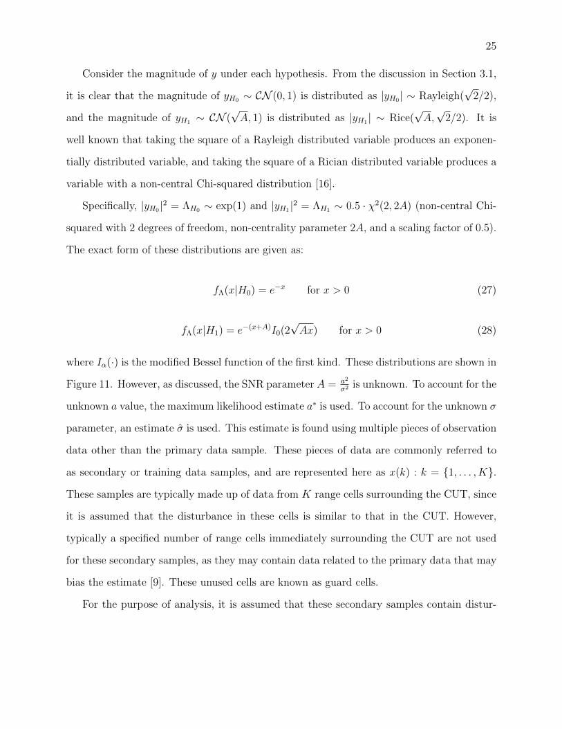
Consider the magnitude of y under each hypothesis. From the discussion in Section 3.1,
it is clear that the magnitude of yH0 ∼ CN (0, 1) is distributed as |yH0| ∼ Rayleigh(√
2/2),
and the magnitude of yH1 ∼ CN (√A, 1) is distributed as |yH1| ∼ Rice(
√A,√
2/2). It is
well known that taking the square of a Rayleigh distributed variable produces an exponen-
tially distributed variable, and taking the square of a Rician distributed variable produces a
variable with a non-central Chi-squared distribution [16].
Specifically, |yH0|2 = ΛH0 ∼ exp(1) and |yH1|2 = ΛH1 ∼ 0.5 · χ2(2, 2A) (non-central Chi-
squared with 2 degrees of freedom, non-centrality parameter 2A, and a scaling factor of 0.5).
The exact form of these distributions are given as:
fΛ(x|H0) = e−x for x > 0 (27)
fΛ(x|H1) = e−(x+A)I0(2√Ax) for x > 0 (28)
where Iα(·) is the modified Bessel function of the first kind. These distributions are shown in
Figure 11. However, as discussed, the SNR parameter A = a2
σ2 is unknown. To account for the
unknown a value, the maximum likelihood estimate a∗ is used. To account for the unknown σ
parameter, an estimate σ is used. This estimate is found using multiple pieces of observation
data other than the primary data sample. These pieces of data are commonly referred to
as secondary or training data samples, and are represented here as x(k) : k = {1, . . . , K}.
These samples are typically made up of data from K range cells surrounding the CUT, since
it is assumed that the disturbance in these cells is similar to that in the CUT. However,
typically a specified number of range cells immediately surrounding the CUT are not used
for these secondary samples, as they may contain data related to the primary data that may
bias the estimate [9]. These unused cells are known as guard cells.
For the purpose of analysis, it is assumed that these secondary samples contain distur-

26
0 10 20 30 40 50 60 70 80 90 100x
0
0.1
0.2
0.3
0.4
0.5
0.6
0.7
0.8
0.9
1
f Λ(x|H
)
fΛ(x|H0)fΛ(x|H1), SNR = 10 dBfΛ(x|H1), SNR = 15 dBfΛ(x|H1), SNR = 18 dB
Figure 11: Probability distributions for the sufficient statistic Λ under hypotheses 0 and 1.The H1 distributions are shown for 3 different SNR values.
bance only. Using these data samples, the sample variance is found as follows:
σ2 =1
K
K∑k=1
|x(k)|2 (29)
Since these secondary samples are all assumed to follow hypothesis 0, x(k) ∼ CN (0, σ2).
Furthermore, each sample can be split into their real parts and imaginary parts, given by
xRe(k) ∼ N (0, σ2
2) and xIm(k) ∼ N (0, σ
2
2) respectively. These variables can each be
rewritten as a scalar times a standard Gaussian random variable:
xRe(k) =
√σ2
2z1(k) xRe(k) =
√σ2
2z2(k)
where z1(k), z2(k) ∼ N (0, 1). Using these statements, the sample variance in equation (29)
can be expanded as:

27
σ2 =1
K
K∑k=1
x2Re(k) + x2
Im(k)
=1
K
K∑k=1
(√σ2
2z1(k)
)2
+
(√σ2
2z2(k)
)2
=σ2
2K
K∑k=1
(z1(k))2 + (z2(k))2
σ2 =σ2
KT (30)
where T = 12
∑Kk=1 (z1(k))2 + (z2(k))2.
Clearly, T is one half of the sum of 2K squared standard Gaussians. It is well known
that the sum of m squared standard Gaussians follows a Chi-squared distribution with m
degrees of freedom [16]. Thus, T must follow a chi-squared distribution with 2K degrees of
freedom that is scaled by 1/2. The exact distribution follows:
fT (t) =2
2K(K − 1)!(2t)K−1e−2t/2
fT (t) =tK−1
(K − 1)!e−t for t > 0 (31)
Now, substituting the σ2 in equation (26) with the estimate σ2 found in (30), we obtain:
|x|2
σ2=K|x|2
σ2T
H1
≷H0
η
Λ
T
H1
≷H0
α (32)
where α = ηK
is the new threshold value, since K is known. Both Λ and T are random
variables, and are assumed to be independent from one another. Their ratio distribution can

28
be found using the following formula [18]:
fZ(z|H) =
∫ ∞−∞|t|fΛ(zt|H)fT (t)dt (33)
where Z = ΛT
. Thus, for the hypothesis 0 case:
fZ(z|H0) =
∫ ∞0
|t|e−zt tK−1
(K − 1)!e−tdt
=1
(K − 1)!
∫ ∞0
tKe−t(1+z)dt
=1
(K − 1)!· K!
(1 + z)K+1
fZ(z|H0) =K!
(1 + z)K+1for z > 0 (34)
For the hypothesis 1 case:
fZ(z|H1) =
∫ ∞0
|t|e−(zt+A)I0(2√
2Azt)tK−1
(K − 1)!e−tdt
=1
(K − 1)!e−A
∫ ∞0
tKe−t(1+z)
∞∑m=0
√Atz
2m
(m!)2dt
=e−A
(K − 1)!
∞∑m=0
(Az)m
(m!)2
∫ ∞0
tK+me−t(1+z)dt
fZ(z|H1) =e−A
(K − 1)!
∞∑m=0
(Az)m
(m!)2
(K +m)!
(1 + z)K+m+1(35)
3.2.3 PFA and PD of detector
To find the probability of false alarm, one must apply equation (20), using equation (34) as
the distribution of the test statistic under hypothesis 0. Thus:
PFA =
∫ ∞α
fZ(z|H0)dz

29
=
∫ ∞α
K!
(1 + z)K+1dz
= (1 + α)−K (36)
Note that the PFA is independent from both the noise variance σ2 and the SNR. In fact, the
probability of false alarm is only dependent on the detection threshold α, and the number
of samples, K, that are used to estimate the noise variance.
Thus, given some number of samples used K, one can set a desired PFA by carefully
choosing the detection threshold α. For a given PFA and K, this choice of α is given as:
α = P−1/KFA − 1 (37)
Note that in order for a detector to be CFAR, it is necessary for the PFA to be independent
of the true interference variance parameter, σ2. In the case of multi-dimensional CFAR
(discussed in Chapter 5), PFA must be independent of the true interference covariance matrix,
Σ.
Similarly, the detection probability is found by applying (22) using (35) as the test
statistic distribution under hypothesis 1:
PD =
∫ ∞α
fZ(z|H1)dz
=
∫ ∞α
e−A
(K − 1)!
∞∑m=0
(Az)m
(m!)2
(K +m)!
(1 + z)K+m+1dz
=e−A
(K − 1)!
∞∑m=0
Am(K +m)!
(m!)2
∫ ∞α
zm
(1 + z)K+m+1dz
=e−A
(K − 1)!
∞∑m=0
(Am(K +m)!
(m!)2
m∑j=0
(K +m− 1− j)!(K +m)!
m!
(m− j)!αm−j
(α + 1)K+m−j
)
=e−A
(K − 1)!
∞∑m=0
(Am
m!
m∑j=0
(K +m− 1− j)!(m− j)!
αm−j
(α + 1)K+m−j
)
=e−A
(K − 1)!
∞∑m=0
(Am
m!
m∑i=0
(K + i− 1)!
i!
αi
(α + 1)K+i
)

30
=e−A
(K − 1)!
∞∑m=0
(Am
m!
m∑i=0
(K − 1)!
(i+K − 1
i
)αi
(α + 1)K+i
)
= e−A∞∑m=0
(Am
m!
m∑i=0
(i+K − 1
i
)(α
α + 1
)i(1
α + 1
)K)
Note that the terms within the second summation((
i+k−1i
) (αα+1
)i ( 1α+1
)K)is the prob-
ability mass function for a negative binomial random variable with parameters K and α1+α
.
Thus, the summation of these terms produces the negative binomial cumulative distribu-
tion function, which has the form of a regularized incomplete Beta function [16]. Thus, the
detection probability can be written as:
PD = e−A∞∑m=0
Am
m!I 1
1+α(K,m+ 1) (38)
where the regularized incomplete beta function is: Ix(a, b) = (a+b−1)!(a−1)!(b−1)!
∫ x0ta−1(1 − t)b−1dt.
Note that other closed forms of equation (38) exist, including a form that does not make use
of an infinite series [19].
The performance of this detector is shown in Figure 12 by displaying the relationship
between PD and SNR. Each curve on this figure shows PD vs SNR for different values of K.
A monotonic relationship between PD and SNR is clearly shown in this figure. Furthermore,
it can be noted that as K increases, the PD vs SNR curve for this detector appears to shift to
the left. This shift implies that at a fixed SNR value, two detectors with different K values
will perform differently. The detector with larger K will have a higher PD.
3.2.4 Performance under Swerling Fluctuation Models
In the above analysis, the SNR is assumed to be a deterministic value. However in certain
applications of radar, the SNR has the tendency to fluctuate and thus behave like a random
variable. Consider a radar whose antenna beam dwells on different targets for a given amount
of time. These periods of time during which the radar is collecting data are called “scans”.

31
0 5 10 15 20 25SNR [dB]
0
0.2
0.4
0.6
0.8
1
PD
K = 10
K = 20
K = 80
Figure 12: PD as a function of SNR (SNR is represented with A in equation (38)) for differentvalues of K for PFA = 1 · 10−6.
Consider also that during each scan, the radar collects data across multiple pulses.
When considering a radar that collects data this way, the fluctuation in SNR is often
thought to follow one of four different cases [20]. First consider a case when the SNR stays
relatively the same across different pulses, but fluctuates across different scans. Secondly,
consider a case when the SNR fluctuates wildly across every single pulse. Swerling cases I
and III describe cases when the fluctuation is from scan to scan, and cases II and IV describe
the pulse to pulse fluctuation. Note also that the type and amount of scatters present also
affects the type of fluctuation. Swerling cases I and II both consider when a target has many
different independent scatterers of about the same size. Swerling cases III and IV both
consider when a target is a combination of one larger scattering surface and many smaller
reflectors [20].
The SNR must now be represented as a random variable. One way to represent the
SNR is γA, where A is a deterministic value representing the average SNR, γ is its random

32
loss/gain multiplier term. Depending on the Swerling case, γ is distributed as [20]:
f(γ) =MM
(M − 1)!γM−1 exp (−Mγ) for γ > 0 (39)
where M =
1 for Swerling I
N for Swerling II
2 for Swerling III
2N for Swerling IV
where N is the spatio-temporal product. Note that N = 1 in the scalar CFAR case.
The detection probability can be found using the same process as before, except using a
different H1 distribution fΛ(x|H1). This distribution can be found by replacing the A term
in equation (28) with γA, then taking the expectation with respect to γ. This process is
shown below for the Swerling I case:
fΛ(x|H1) = E[e−(x+γA)I0(2
√Aγx)
]=
∫ ∞0
e−(x+γA)
∞∑m=0
(γAx)m
(m!)2f(γ)dγ
= e−x∞∑m=0
(Ax)m
(m!)2
∫ ∞0
e−γ(A+1)γmdγ
= e−x∞∑m=0
(Ax)m
(m!)2
m!
(1 + A)m+1
=e−x
1 + A
∞∑m=0
1
m!
(Ax
1 + A
)m=
e−x
1 + Aexp
(Ax
1 + A
)=
1
1 + Aexp
(−x
1 + A
)(40)
Since the conditional distribution for Λ depends on the unknown parameter σ (by merit
of A), the conditional distribution for the variable Z = ΛT
is found instead, as in equation (33)

33
(since Z is instead dependent on the estimated σ). This new test statistic Z is distributed
as follows:
fZ(z|H1) =
∫ ∞0
|t| 1
1 + Aexp
(−zt
1 + A
)tK−1
(K − 1)!e−tdt
=1
(K − 1)!(1 + A)
∫ ∞0
e−t(1+A+z
1+A )dt
=1
(K − 1)!(1 + A)· K!(
1+A+z1+A
)K+1
=K(1 + A)K
(1 + A+ z)K+1(41)
Finally, equation (22) is used to find the detection probability, using the fZ(z|H1) term
found in (41) as the distribution of the target + interference:
PD,Swerling I =
∫ ∞α
K(1 + A)K
(1 + A+ z)K+1dz
= K(1 + A)K[−1
K(1 + A+ z)−K
]∞α
=
(1 + A
1 + A+ α
)K(42)
This formulation for PD is much less cumbersome than PD for the non-fluctuating case,
shown in (38). The PD for the Swerling III case can also be found, using a very similar
process. While the steps are not shown here, the final form of PD under Swerling III is given
as follows:
PD,Swerling III =
(2 + A
A+ 2(1 + α)
)K+1(1 +
2α(2 + A(1 +K))
(2 + A)2
)(43)
Note that the Swerling fluctuation models only affect the SNR parameter A. Since A
is not used in the derivation of the PFA or the detection threshold α, these values are the
same as the formulations in (36) and (37), regardless of which fluctuation model is being

34
0 5 10 15 20 25 30 35SNR [dB]
0
0.2
0.4
0.6
0.8
1
PD
Non-fluctuating
Swerling I
Swerling III
Figure 13: PD vs SNR curves shown for the Swerling I, Swerling III, and non-fluctuatingcase for K = 10 and PFA = 10−4. Note that the PD vs SNR curves for Swerling II andSwerling IV are equal to that of Swerling I and Swerling III respectively when scalar datasamples are used.
used. The same statement applies to the 0 hypothesis distributions, fΛ(x|H0) in (27) and
fZ(z|H0) in (34). The relationship between PD and SNR for the different Swerling cases are
shown in Figure 13.

Chapter 4
Robust Decision Making for Ordered
Statistic CFAR
4.1 Ordered Statistic CFAR
So far, the analysis of PFA and PD for scalar CFAR has assumed that the secondary samples
x(k) are independent and identically distributed as noise/interference. Because of this, it’s
simple to estimate the variance of this noise/interference by using sample variance, as in
(29). This can also be thought of as taking the mean value of y(k) = |x(k)|2:
σ2 =1
K
K∑k=1
y(k)
These y(k) samples are obtained by applying a square law detector on the secondary samples
x(k) [9]. Since the detection scheme uses a statistic, σ2, that is a sample average of these
y(k) data samples, the detection scheme discussed in section 3.2 is commonly known as cell
averaging CFAR (CA-CFAR) [9].
Unfortunately, while a sample average is easy to implement, it is very susceptible to
producing poor estimates when the secondary data have outliers or samples that are not
identically distributed. Furthermore, in practice, many scenarios arise where secondary
35

36
samples are distributed differently. One such scenario is when the clutter interference comes
from different sources (such as different terrain or scatterer types) [6]. Another scenario
is when some of the secondary samples contain target information. These differing clutter
types and interfering targets cause the secondary samples to be non-homogeneous which is
known to degrade detection performance [21].
When secondary samples contain non-homogeneous data, the sample variance σ2 given
in (29) no longer provides an accurate estimate for the variance of the disturbance in the
primary data sample. Thus, other methods of estimating this variance are used which aim
to be more robust when these heterogeneities exist in the secondary data. One such method
orders the secondary data samples by their size, and selects the mth largest value as the
interference estimate. This method is known as ordered statistic CFAR (OS-CFAR).
4.1.1 OS-CFAR performance
The assumptions on noise used in Section 3.2.1 are used in this section as well. Specifically, it
is assumed that the interference follows a complex Gaussian distribution, and is independent
from sample to sample. It has been shown that this detector has the CFAR property when the
interference follows an exponential distribution [6]. As we have shown in previous sections,
if x ∼ CN (0, σ2), then |x|2 ∼ exponential(1/σ2). Thus, let the primary data sample be
represented as z = |x|2. Similarly, let the secondary data samples be represented as z(k) =
|x(k)|2 for k = {1, . . . , K}.
Out of the K secondary samples, let the random variable T represent the value of the
mth highest value. The hypothesis test for OS-CFAR is defined as [6]:
zH1
≷H0
Tα (44)
where α is a constant, scalar multiplier term. Note that there are random variables on both
sides of this inequality, since both z and T are random. It is entirely possible to put both

37
random variables on the same side of the inequality, to obtain a single detection statistic in
the form of the ratio zT
. However, the PDF for zT
does not easily admit a closed form. Thus,
instead, the PFA is calculated as follows:
PFA|T=t =
∫ ∞tα
fz(z|H0)dz (45)
where fz(·) is the distribution of z, and PFA|T=t is the probability of false alarm given that
the random variable T is equal to the value t.
Thus, to find PFA, one can take the expectation of PFA|T=t across T :
PFA = ET
[PFA|T=t
]=
∫ ∞−∞
(fT (t)
∫ ∞tα
fz(z|H0)dz dt
)(46)
Similarly, the detection probability PD has the form:
PD =
∫ ∞−∞
(fT (t)
∫ ∞tα
fz(z|H1)dz dt
)(47)
From (46) and (47), PFA and PD can be calculated as long as fT (t), fz(z|H0) and fz(z|H1)
are known.
Recall from equation (26) that Λ = |x|2σ2 , which implies that z = Λσ2. Thus, fz(z|Hi) is
just a scaled version of fΛ(x|Hi), with a scaling coefficient of σ2:
fz(z|Hi) =1
σ2fΛ
(z
σ2
∣∣∣∣Hi
)
This equation can be applied to equations (27) and (40), yielding:
fz(z|H0) =1
σ2exp
(−z/σ2
)(48)

38
fz(z|H1) =1
σ2(1 + A)exp
(−z
σ2(1 + A)
)(49)
Note that equation (28) can be also be used to solve for fz(z|H1). However, (40) is used here
since it is less cumbersome and more easily yields a closed form for the detection probability.
Recall that T represents the secondary sample with themth largest value. The assumption
that all secondary samples are independent, and identically distributed as interference only is
used for this derivation as well. For a collection of K independent and identically distributed
random variables, the probability distribution of the mth largest value is as follows[16]:
fT (t) = fm(z) = m
(K
m
)[1− F (z(k))]K−m [F (z(k))]m−1 f(z(k)) (50)
where F (z(k)) is the cumulative distribution function of z(k), and f(z(k)) is the probability
density function of z(k). Since these secondary samples follow the noise only hypothesis,
f(z) has the same distribution as (48), which has a cumulative distribution of:
F (z(k)) = 1− exp(−z/σ2)
Using these distributions, fT (t) is found to be:
fT (t) = m
(K
m
)[exp
(−tσ2
)]K−m [1− exp
(−tσ2
)]m−11
σ2exp
(−tσ2
)fT (t) =
m
σ2
(K
m
)[exp
(−tσ2
)]K−m+1 [1− exp
(−tσ2
)]m−1
for t > 0 (51)
Thus, PFA is:
PFA =
∫ ∞0
m
σ2
(K
m
)[exp
(−tσ2
)]K−m+1 [1− exp
(−tσ2
)]m−1 ∫ ∞tα
1
σ2exp
(−y/σ2
)dy dt
=m
σ2
(K
m
)∫ ∞−∞
[exp
(−tσ2
)]K−m+1 [1− exp
(−tσ2
)]m−1
exp
(−αtσ2
)dt
=m
σ2
(K
m
)∫ ∞−∞
exp
(−tσ2
(K −m+ 1 + α)
)[1− exp
(−tσ2
)]m−1
dt (52)

39
Consider the change of variables: x = tσ2 =⇒ dx = dt
σ2 :
PFA = m
(K
m
)∫ ∞−∞
exp (−x(K −m+ 1 + α)) [1− exp (−x)]m−1 dx
=m−1∏i=0
K − iK − i+ α
(53)
PD is found in this same manner. Since both (48) and (49) are exponentially distributed,
the derivation is very similar and is excluded here. The equation for PD is as follows:
PD =m−1∏i=0
K − iK − i+ α
1+A
(54)
For the CA-CFAR case, a closed form for α given some desired PFA value was obtained
in equation (37). However, in the OS-CFAR case, the threshold term given a desired PFA
must be obtained from equation (53), which does not easily permit a closed form. However,
PFA monotonically decrease in α, thus numerical methods, such as line search or Newton’s
method can be used to solve for α given a desired PFA. Below, Table 1 shows selected values
of α that have been numerically obtained using a MATLAB routine involving a line search
method.
Using these numerically calculated threshold values, equation (54) is used to calculate
the PD as a function of m at different SNR values. This relationship is shown in Figure
14. From this figure, it’s clear that the detection probability is quite poor at low m. As m
increases, however, the PD begins to rise up to a maximum point. Eventually, the PD begins
to decrease again as m nears K.
Figure 14 shows the particular case of K = 24 and PFA = 1 · 10−4. In this case, the PD
reaches a maximum around m = 20, or m = 21, depending on the SNR. As shown in the
figure, the PD surrounding the maximum are very close in value. Much of the literature on
OS-CFAR agrees that, while the maximum PD occurs at around m = 7K/8, it is better to
use a value of m = 3K/4, since it allows for the censoring of more interfering targets [6],[22].
40
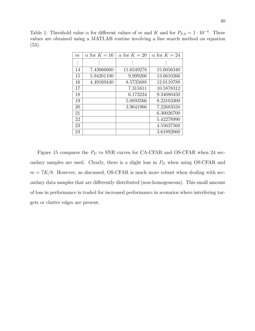
Table 1: Threshold value α for different values of m and K and for PFA = 1 · 10−4. Thesevalues are obtained using a MATLAB routine involving a line search method on equation(53).
m α for K = 16 α for K = 20 α for K = 24...
......
...14 7.43066660 11.6549278 15.605634015 5.94201100 9.999266 13.661026616 4.49169440 8.5735688 12.011078817 7.315811 10.587831218 6.173234 9.3408045019 5.0893566 8.2310330020 3.9641966 7.2268355021 6.3002670022 5.4227899023 4.5563756024 3.61892660
Figure 15 compares the PD vs SNR curves for CA-CFAR and OS-CFAR when 24 sec-
ondary samples are used. Clearly, there is a slight loss in PD when using OS-CFAR and
m = 7K/8. However, as discussed, OS-CFAR is much more robust when dealing with sec-
ondary data samples that are differently distributed (non-homogeneous). This small amount
of loss in performance is traded for increased performance in scenarios where interfering tar-
gets or clutter edges are present.

41
2 4 6 8 10 12 14 16 18 20 22 24m
0
0.05
0.1
0.15
0.2
0.25
0.3
0.35
PD
SNR = 5 dBSNR = 6 dBSNR = 7 dBSNR = 8 dBSNR = 9 dBSNR = 10 dB
Figure 14: PD vs m for K = 24 and PFA = 1 · 10−4, shown for different SNR values.
0 5 10 15 20 25 30SNR [dB]
0
0.1
0.2
0.3
0.4
0.5
0.6
0.7
0.8
0.9
1
PD
OS-CFAR, m = 20
CA-CFAR
Figure 15: PD vs SNR for K = 24 and PFA = 1 · 10−4 for the Swerling I case, shown forboth CA-CFAR.

42
4.1.2 Effects of Interfering targets
Note that equations (53) and (54) provide formulations for the PFA and PD when all sec-
ondary samples are homogeneous and disturbance only. While OS-CFAR has been proposed
as an algorithm with increased robustness towards non-homogeneous secondary samples, the
effects of non-homogeneous secondary samples still cause the PD and PFA to suffer. In par-
ticular, the effects of the secondary samples containing interfering targets are observed in
this section.
Let J represent the number of interfering targets present within the secondary samples.
Consider that each interfering target has a relative signal strength (RSS), which must also
be taken into account. Note that equation (50) provides the probability distribution for
the mth largest secondary sample, assuming that all secondary samples are independent
and identically distributed. The distribution of the mth largest secondary sample when the
secondary samples are independent but not necessarily identically distributed is given as
follows [23]:
gm(t) =1
(m− 1)!(K −m)!
∑p
Fi1(t)...Fim−1(t) · fim(t) · {1− Fim+1(t)}...{1− FiK (t)} (55)
where Fi1 , . . . , FiK and fi1 , . . . , fiK respectively represent the CDFs and PDFs of the K
different secondary samples. Note that i1, i2, . . . , iK represent different possible orderings of
1, 2, . . . , K, and∑
p represents the summation over every possible permutation of i1, i2, . . . , iK .
Note that K! total permutations exist for a list of length K, and thus there is an extremely
large number of summed terms in (55) for large K. However, this number of summed
terms is reduced if one considers that the secondary samples containing disturbance are
identically distributed. Furthermore, the number of summed terms is reduced even further
if the assumption is made that each interfering target has the same RSS [24].
Given these assumptions, each secondary sample containing an interfering target follows
hypothesis 1, and has the PDF given in (49). Similarly, each secondary sample containing

43
disturbance follows hypothesis 0 and has the distribution shown in (48). Thus:
f0(t) =1
σ2exp(−t/σ2) (56)
f1(t) =1
σ2(1 + A)exp
(−t
σ2(1 + A)
)(57)
F0(t) = 1− exp(−t/σ2) (58)
F1(t) = 1− exp
(−t
σ2(1 + A)
)(59)
where f0(t) and F0(t) represent the distributions of the secondary samples containing distur-
bance, and f1(t) and F1(t) represent the distributions of the secondary samples containing
interfering targets, and A is the RSS of the interfering targets.
Thus, now that the distributions in (55) are represented by a combination of J zeros
and K − J ones, not every permutation of i1, i2, . . . , iK will be unique. In fact, out of the
K! permutations of J zeros and K − J ones, only(KJ
)of them are unique. Note that each
of these unique permutations are repeated a total of J !(K − J)! times, thus resulting in(KJ
)· J !(K − J)! = K! total permutations. Furthermore, since (55) considers the product of
repeated terms, the number of summed terms in (55) is reduced even further. By taking all
of these observations into account, the following formulation of gm(t) is written:
gm(t) =J !(K − J)!
(m− 1)!(K −m)!
{ min(m−1,J)∑`2=max(0,J−K+m)
F `21 Fm−1−`20 · f0 · {1− F1}J−`2{1− F0}K−m−J+`2
(m− 1
`2
)(K −mJ − `2
)
+
min(m−1,J−1)∑`1=max(0,J−1−K+m)
F `11 Fm−1−`10 · f1 · {1− F1}J−1−`1{1− F0}K−m−J+1+`1
(m− 1
`1
)( K −mJ − 1− `1
)}(60)
As this is the distribution for the mth largest secondary sample, it can be used to find
the PD of the OS-CFAR detector via (47) as follows:
PD =
∫ ∞0
gm(t)
∫ ∞tα
1
σ2(1 + A)exp
(−t
σ2(1 + A)
)dt
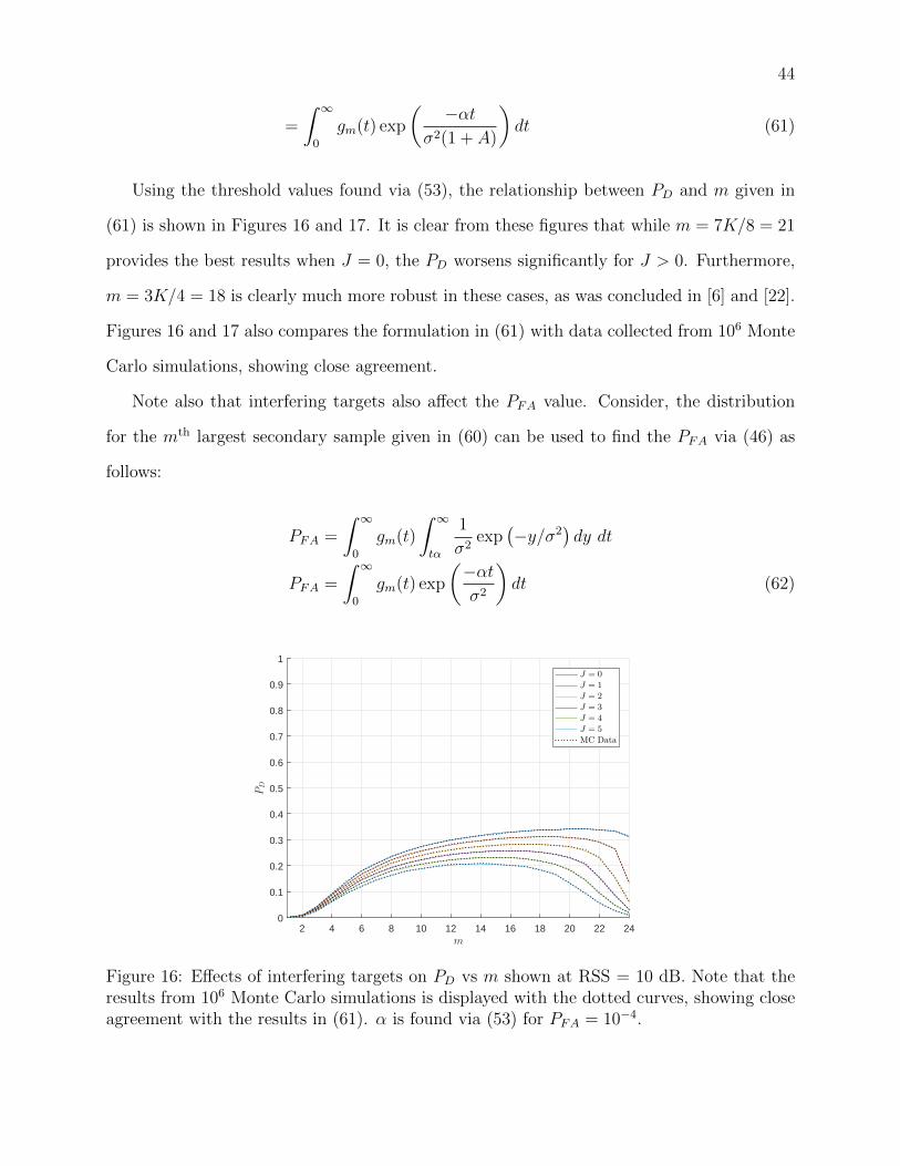
44
=
∫ ∞0
gm(t) exp
(−αt
σ2(1 + A)
)dt (61)
Using the threshold values found via (53), the relationship between PD and m given in
(61) is shown in Figures 16 and 17. It is clear from these figures that while m = 7K/8 = 21
provides the best results when J = 0, the PD worsens significantly for J > 0. Furthermore,
m = 3K/4 = 18 is clearly much more robust in these cases, as was concluded in [6] and [22].
Figures 16 and 17 also compares the formulation in (61) with data collected from 106 Monte
Carlo simulations, showing close agreement.
Note also that interfering targets also affect the PFA value. Consider, the distribution
for the mth largest secondary sample given in (60) can be used to find the PFA via (46) as
follows:
PFA =
∫ ∞0
gm(t)
∫ ∞tα
1
σ2exp
(−y/σ2
)dy dt
PFA =
∫ ∞0
gm(t) exp
(−αtσ2
)dt (62)
2 4 6 8 10 12 14 16 18 20 22 24m
0
0.1
0.2
0.3
0.4
0.5
0.6
0.7
0.8
0.9
1
PD
J = 0J = 1J = 2J = 3J = 4J = 5MC Data
Figure 16: Effects of interfering targets on PD vs m shown at RSS = 10 dB. Note that theresults from 106 Monte Carlo simulations is displayed with the dotted curves, showing closeagreement with the results in (61). α is found via (53) for PFA = 10−4.

45
The effects of interfering targets on the PFA is shown in Figure 18. The data in this figure
uses an α that is calculated via (53) for PFA = 10−4. Note that this α works as intended in
the case when there are no interfering targets, and the PFA is set to be a constant value of
10−4. However, the PFA begins to decrease below the prescribed value of 10−4 as interfering
targets are introduced. Note that a lower PFA value is also associated with a lower PD value,
as explained in Section 3.1.4. Part of this loss in PD is observed in Figures 16 and 17.
4.2 Information Elasticity Framework for OS-CFAR
Consider, given a fixed K, the PD and PFA of a OS-CFAR detector are generally a function
of four different variables. Two of these variables are parameters that the decision maker
has control of, namely the threshold α and the order statistic parameter m. The remaining
two variables are environmental parameters that are typically unknown to a decision maker:
the number of interfering targets J and the RSS of said targets.
Ideally, the decision maker would be able to select the decision variables (α and m) to be
able to fix the PFA at a constant value while also providing a satisfactory PD, as is the goal
2 4 6 8 10 12 14 16 18 20 22 24m
0
0.1
0.2
0.3
0.4
0.5
0.6
0.7
0.8
0.9
1
PD
J = 0J = 1J = 2J = 3J = 4J = 5MC Data
Figure 17: Effects of interfering targets on PD vs m shown at RSS = 20 dB. Note that theresults from 106 Monte Carlo simulations is displayed with the dotted curves, showing closeagreement with the results in (61). α is found via (53) for PFA = 10−4.

46
of many CFAR detectors. Unfortunately, this task is difficult to accomplish if the number
of interfering targets and their associated RSS values are unknown. Fortunately, methods,
such as the Forward Automatic Order Selection Ordered Statistics Detector (FAOSOSD)
[25], have been proposed to provide an estimate for the number of interfering targets present.
However, the accuracy of the estimate provided by the FAOSOSD algorithm has been shown
to depend on the RSS of the interfering targets [4]. Thus, while a decision may be suitable at
one value of RSS, it may not necessarily be suitable at a different value. Thus, an information
elasticity framework is proposed to improve the system’s robustness to the variations in
RSS. In this section, the performance of the FAOSOSD estimate is analyzed, a performance
function is defined, and a measure of robustness and absolute performance are determined.
4.2.1 Estimation of J using FAOSOSD
In [25], an estimation technique known as information theoretic criteria (ITC) is used to find
an estimate for J (denoted by J). ITC are generally used to compare different statistical
models. The ITC provide a measure of quality for these different models, given a set of
observations [26], [27]. These criteria were first used in a signal detection application in [28],
2 4 6 8 10 12 14 16 18 20 22 24m
10-8
10-7
10-6
10-5
10-4
10-3
PFA
J = 0J = 1J = 2J = 3J = 4J = 5
Figure 18: Effects of interfering targets on PFA vs m for RSS = 10 dB. α is found via (53)for PFA = 10−4.

47
where ITC were used to estimate the number of signals present in observed multichannel
time-series data. This technique is applied in the FAOSOSD [25], comparing different models
describing the number of interfering targets present.
One particular type of ITC is known as minimum description length (MDL), and is first
given in [27]. The form of the MDL used in the FAOSOSD is given as [25]:
MDL(n) = −(K − n)K ln
(G(λn+1, . . . , λK)
A(λn+1, . . . , λK)
)+
1
2n(2K − n) ln(K) (63)
where λ1 ≥ λ2 ≥ . . . ≥ λK represent the ordered secondary samples, and G(·, . . . , ·) and
A(·, . . . , ·) represent the geometric and algebraic means of their arguments, respectively.
The value of n at which MDL(n) reaches a minimum (denoted as n∗) is considered to be the
model that best fits the observed data, and the K − n∗ + 1 largest samples are assumed to
come from interfering targets [14]. Thus, the estimated number of interfering targets is:
J = K − argmaxn
[MDL(n)] + 1 (64)
Using Monte Carlo simulations, the general performance of this algorithm is approxi-
mated. FAOSOSD is used to estimate J for K simulated secondary samples where J inter-
fering targets are present. This process is repeated in 106 separate Monte Carlo simulations.
Using the relative frequencies of J , the conditional probability mass function P (J |J) is ap-
proximated for 1 ≤ J ≤ K and 1 ≤ J ≤ K. This represents the probability of the FAOSOSD
estimating J given that J interfering targets exist. Using Bayes’ rule:
P(J |J) =P(J)P(J |J)∑KJ=0 P(J)P(J |J)
where P (J |J) represents the a posteriori PMF, describing the probability that J interfering
targets are present given that the FAOSOSD has estimated J . P (J) represents the a priori
PMF of J . If this knowledge of J is unknown to a user, then ignorance may be assumed,

48
and each value of J is considered equally likely to occur. In this case, a uniform distribution
is assumed for P (J), yielding the following:
P (J |J) =P(J |J)∑KJ=0 P(J |J)
This a posteriori PMF is shown for J = 5 and K = 20 in Figure 19. This figure
shows that at an RSS of 20 dB, the probability of correctly estimating J is larger than the
probability incorrectly estimating, i.e. P (J = 5|J = 5) > P (J 6= 5|J = 5). However, as
the RSS decreases to 17 dB, the probability of correctly estimating J decreases, and now
P (J = 5|J = 5) < P (J 6= 5|J = 5). The probability of correctly estimating J drops even
further when RSS is decreased to 7 dB. In general, Monte Carlo simulations have shown that
the FAOSOSD becomes more likely to correctly estimate J as the RSS increases.
0 2 4 6 8 10 12 14 16 18 20J
0
0.5
1
P(J
|J=
5)
0 2 4 6 8 10 12 14 16 18 20J
0
0.5
1
P(J
|J=
5)
0 2 4 6 8 10 12 14 16 18 20J
0
0.5
1
P(J
|J=
5)
RSS = 20 dB
RSS = 17 dB
RSS = 7 dB
Figure 19: P (J |J) shown for K = 20 and different RSS values.
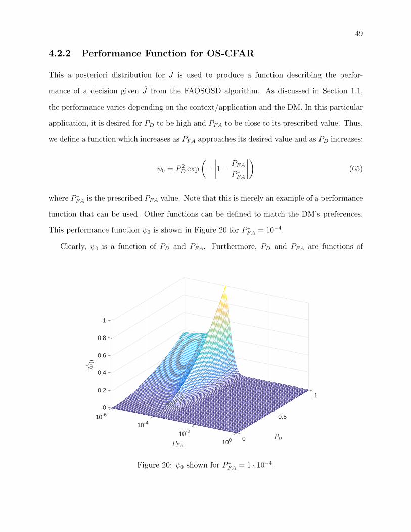
49
4.2.2 Performance Function for OS-CFAR
This a posteriori distribution for J is used to produce a function describing the perfor-
mance of a decision given J from the FAOSOSD algorithm. As discussed in Section 1.1,
the performance varies depending on the context/application and the DM. In this particular
application, it is desired for PD to be high and PFA to be close to its prescribed value. Thus,
we define a function which increases as PFA approaches its desired value and as PD increases:
ψ0 = P 2D exp
(−∣∣∣∣1− PFA
P ∗FA
∣∣∣∣) (65)
where P ∗FA is the prescribed PFA value. Note that this is merely an example of a performance
function that can be used. Other functions can be defined to match the DM’s preferences.
This performance function ψ0 is shown in Figure 20 for P ∗FA = 10−4.
Clearly, ψ0 is a function of PD and PFA. Furthermore, PD and PFA are functions of
1
0
10-6
PD
0.5
0.2
0.4
10-4
PFA
ψ0
0.6
10-2
0.8
0
1
100
Figure 20: ψ0 shown for P ∗FA = 1 · 10−4.

50
α, m, J , and RSS, as discussed in Section 4.1.2. Thus, ψ0 is also a function of these four
variables. Let the decision variables α and m be contained in the vector x = (α,m). The
performance function can thus be represented as ψ0(x, J,RSS). To account for the fact that
J is unknown, the conditional mean of this performance function is obtained using the a
posteriori distribution of J , as follows:
ψJ(x,RSS) =K∑j=0
ψ0(x, J,RSS)P (J |J ,RSS) (66)
This conditional mean can also be thought of as a weighted sum of ψ0 values. The perfor-
mance ψ0(x, J,RSS) is weighted more if J is more probable, given the estimate J .
4.2.3 Robust decision making method
ψJ(x,RSS) provides a relative measure for performance of a decision x at a specific RSS
value. However, as discussed, the RSS of the interfering targets is unknown. Let A =
{A1, A2, . . . , AM} represent a vector containing M possible RSS values for the interfering
targets. The goal is to select a decision x that generally performs well at the RSS values
within A (increased absolute performance), while also reducing the sensitivity of the per-
formance function to these RSS values (increased robustness). The concepts of absolute
performance and robustness are characterized using the mean and variance of a performance
metric respectively, in [29]. Thus, the sample mean and variance across values in A are used
in this framework to represent absolute performance and the robustness respectively. The
sample mean and sample variances of ψJ(x,RSS) are obtained across these RSS values as
follows:
µ(x,A) =1
M
M∑i=1
ψJ(x, Ai) (67)
Var(x,A) =1
M − 1
M∑i=1
|ψJ(x, Ai)− µ(x,A)|2 (68)

51
The µ(x,A) and Var(x,A) for many different decision points are shown in Figure 21.
Consider, it is desired for µ(x,A) to be high and Var(x,A) to be low. With this in mind,
there is a clearly defined Pareto frontier for these decision points. Looking at these Pareto
efficient solutions only, a clear trade-off between absolute performance and robustness is
observed.
To select a decision that balances these trade-offs, the normalized distance from the
utopia point is used as a measure of decision effectiveness, E, as discussed in Section 2.2.
This measure is given as follows:
E =
[ µ−maxx
(µ)
maxx
(µ)
]2
+
Var
maxx
(Var)
21/2
(69)
The decision effectiveness is shown as a function of Var in Figure 21. Clearly, as the
measure of robustness improves (Var decreases), the decision effectiveness improves (E de-
0 0.005 0.01 0.015 0.02 0.025 0.03 0.035 0.04Var(x,A)
0
0.05
0.1
0.15
0.2
0.25
0.3
0.35
μ(x,A
)
Figure 21: µ(x,A) vs Var(x,A) shown for J = 5, N = 20, and P ∗FA = 10−4. Points shownfor 8400 decision points and A = {5, 10, . . . , 90, 95}. Pareto frontier is shown by the blackcurve.

52
creases). Eventually, a minimum/overload point is reached. Decreasing Var beyond this
overload point only causes the decision effectiveness to get worse. Thus, information over-
load is observed using this framework, allowing the DM to select the decision with the
maximum decision effectiveness. For this particular example, the overload point is reached
when Var = 0.4577, which occurs at the decision m = 12 and α = 8.8940.
0 0.005 0.01 0.015 0.02 0.025 0.03 0.035 0.04Var(x,A)
0.4
0.5
0.6
0.7
0.8
0.9
1
E
Figure 22: Decision effectiveness shown as a function of the measure of robustness, Var.Note that the overload point occurs at the decision m = 12 and α = 8.8940.

Chapter 5
Information Elasticity Framework for
the AMF
Chapters 3 and 4 discussed detectors where the primary and secondary samples consist
of scalar values. This chapter focuses on the adaptive matched filter (AMF), where these
primary and secondary samples are each N × 1 vectors, where N is the dimensionality,
or the spatio-temporal product (as was briefly discussed in Chapter 1). With data being
N -dimensional, the behavior of the disturbance is now characterized using a multivariate
complex Gaussian distribution. This distribution considers an N × 1 mean vector and an
N ×N covariance matrix, represented by Σ.
Just as the scalar CFAR detector discussed in Section 3.2 used a test statistic involving
an estimate for σ2, the AMF uses a test statistic involving an estimate for Σ. Two methods
of estimating Σ are analyzed in this paper, namely sample matrix inversion (SMI) and rank
constrained maximum likelihood estimation (RCML). These methods each produce an esti-
mate from K secondary samples, and when these samples assumed to be homogeneous and
disturbance only, the performance of the AMF improves as K increases, up to a theoretical
limit [30]. This limit is the performance of a detector, known as the clairvoyant detector
where the disturbance covariance matrix is known.
53
54
While increasing K provides improved performance when secondary samples are assumed
to be homogeneous and target free, in practice, this choice of K is often constrained due to
the fact that only a certain number of homogeneous training samples are available within
a given environment. Unfortunately, radar data is often non-homogeneous in practice, and
increasing K increases the likelihood that the training samples contain a non-homogeneity
[9] [31], such as an interfering target or different clutter type. As these non-homogeneities
cause the detection performance to suffer, a high number of training samples is undesirable.
Thus, a DM must consider these trade-offs when selecting K.
This chapter develops an information elasticity framework for selecting decision param-
eters for the AMF. In this framework, the decision quality metric is based on a comparison
between the AMF performance and the clairvoyant detector performance. The clairvoyant
detector is based on the likelihood ratio test, which is derived in [32] and [8] and included
in section 5.1 for completeness. The PD for the AMF is originally derived in [8], and the
derivation is given in Section 5.2 for completeness. In this chapter, we define a constraint
function with user-tunable parameters, allowing a DM to specify the level of cost associ-
ated with using different decisions. Using this framework, information overload is observed,
allowing the DM to select cost-efficient solutions.
5.1 Clairvoyant Detector
5.1.1 Likelihood Ratio Test
As discussed, the primary data now takes the form of a N ×1 vector, represented by x. Just
as in Section 3.2, this observed data must follow one of two hypotheses:
H0 : x = n
H1 : x = sa+ n

55
where H0 is the disturbance only hypothesis and H1 is the target + disturbance hypothesis.
The n vector is assumed to follow a multivariate complex Gaussian distribution with mean 0
and a covariance matrix Σ. Furthermore, a is the same deterministic and unknown complex
scalar introduced in Section 3.2.1, and s is the steering vector, which is deterministic and
known.
Just as in Section 3.2.1, the detection test is set up using the likelihood ratio. The
conditional distributions of the observation vector are given as [17]:
fx|H1(x|H1,Σ) =1
πN |Σ|e−(x−as)HΣ−1(x−as)
fx|H0(x|H0,Σ) =1
πN |Σ|e−x
HΣ−1x
Again, the ratio of these conditional distributions is taken, and its natural log is considered:
Λ(x) = exHΣ−1x−(x−as)HΣ−1(x−as)
σ2
Λ(x) = ln Λ(x) = xHΣ−1x− (x− as)HΣ−1(x− as)
Λ(x) = 2Re(a∗sHΣ−1x
)− |a|2sHΣ−1s (70)
Again, the maximum likelihood estimator for a is obtained via differentiation:
∂
∂aΛ(x) =
(2sHx− 2asHs
)= 0
2sHΣ−1x = 2asHΣ−1s
a∗ =sHΣ−1x
sHΣ−1s
where a∗ is the maximum likelihood estimate of a. Substituting this in for a in equation (70)
56
yields:
Λ(x) = 2
(sHΣ−1x
sHΣ−1s
)∗sHΣ−1x−
∣∣∣∣sHΣ−1x
sHΣ−1s
∣∣∣∣2 sHΣ−1s
=
(2
∣∣sHΣ−1x∣∣2
sHΣ−1s−∣∣sHΣ−1x
∣∣2sHΣ−1s
)
Λ(x) =
∣∣sHΣ−1x∣∣2
sHΣ−1s
H1
≷H0
η (71)
This is the likelihood ratio test for the observed primary data vector when the true covariance
matrix Σ is known. Thus, Λ(x) is used as the sufficient statistic for the clairvoyant detector.
The distribution for Λ(x) is given in the following subsection.
5.1.2 PD and PFA of Clairvoyant Detector
Let y = sHΣ−1x√sHΣ−1s
. Clearly, the test statistic in (71) can be rewritten as Λ(x) = |y|2. Further-
more, let w = Σ−1s√sHΣ−1s
, which is clearly a deterministic N × 1 vector. Consider, y = wHx.
Thus y can be thought of a linear combination of elements in x, which follow a multivariate
complex Gaussian distribution. It is well known that a linear combination of Gaussian ran-
dom variables also produces a Gaussian random variable [16], and thus y must be Gaussian.
Although y is known to be Gaussian, its mean and variance depend on which hypothesis
is being considered. For H0, the mean and variance are found as follows:
E [y|H0] = E[wHx|H0
]= wH · E [x|H0] = 0
Var(y|H0) = E(|wHx|2 |H0)− E(wHx |H0)2
= E(wHxxHw |H0)− 0
= wHE(xxH |H0)w
57
= wHΣw
=sHΣ−1ΣΣ−1s
sHΣ−1s= 1.
Thus, y ∼ CN (0, 1) under hypothesis 0. Similarly:
E [y|H1] = E[wHx|H1
]= wH · E [x|H1] = wHas
= awHs
Var(y|H1) = E[|wHx|2 |H1
]− E
[wHx|H1
]2= wHE
[xxH |H1
]w − a2wHssHw
= wHE[(as− n)(as− n)H
]w − a2wHssHw
= wHE[a2ssH + 2asnH + nnH
]w − a2wHssHw
= wH
[a2ssH + 2as
�����*0
E(nH)
+ E(nnH)
]w − a2wHssHw
=������a2wHssHw + wHΣw −����
��a2wHssHw = 1
Thus, y ∼ CN (awHs, 1) under hypothesis 1.
Consider, the w vector can be thought of as filter weights, x can be thought of as the
input of the filter, and y = wHx can be thought of as the output of the filter. Furthermore,
now that the distribution of y under both hypotheses is known, the following can be written:
H0 : y = n
H1 : y = awHs+ n
58
where n ∼ CN (0, 1). Using this consideration, the SNR of this output signal can be found
the same way as in Section 3.2.2:
SNR = A =|awHs|2
E(n2)
=|a|2wHssHw
1
= |a|2 sHΣ−1ssHΣ−1s
sHΣ−1s
= |a|2sHΣ−1s (72)
Furthermore, it’s clear that√A = awHs, thus y ∼ CN (0, 1) under hypothesis 0 and y ∼
CN (√A, 1) under hypothesis 1. From the discussion in Section 3.2.2, Λ(x) = |y|2 clearly is
exponentially distributed under hypothesis 0 and follows a non-central χ2 distribution under
hypothesis 1, as follows:
fΛ|H0(t) = e−t for t > 0 (73)
fΛ|H1(t) = e−(t+A)I0(2√At) for t > 0 (74)
Thus, using equation (20), the PFA for the clairvoyant detector is as follows:
PFA =
∫ ∞η
e−tdt
PFA = e−η (75)
where η is the threshold term given in (71). For this detector, the PFA can be set to a
desired value by setting the threshold term to η = − ln(PFA). Using (22), PD can be found
as follows:
PD =
∫ ∞η
e−(t+A)I0(2√At) dt
= e−A∫ ∞η
e−t∞∑m=0
(√At)2m
(m!)2dt
59
= e−A∞∑m=0
Am
m!
∫ ∞η
tme−t
m!dt
= e−A∞∑m=0
Am
m!Γ(η,m+ 1) (76)
where Γ(η,m+ 1) =∫∞η
tme−t
m!dt is the normalized upper incomplete gamma function. Note
that both the PFA and PD for these detectors are independent of the dimensionality N .
If the Swerling I model is assumed, the random SNR fluctuation term distributed by (39)
is applied, and the expectation is taken:
PD,Swerling I = Eγ
[e−Aγ
∞∑m=0
(Aγ)m
m!Γ(η,m+ 1)
]
=∞∑m=0
Eγ[e−Aγγm
] Amm!
∫ ∞η
tme−t
m!dt
=∞∑m=0
[∫ ∞0
e−γ(A+1)γm]Am
m!
∫ ∞η
tme−t
m!dt
=∞∑m=0
m!
(1 + A)m+1
Am
m!
∫ ∞η
tme−t
m!dt
=
∫ ∞η
e−t
1 + A
∞∑m=0
1
m!
(At
1 + 1
)mdt
=1
1 + A
∫ ∞η
e−tet(A/(1+A))dt
= e−η/(1+A) (77)
5.2 Adaptive Matched Filter
The AMF uses the likelihood ratio test given in (71) and replaces the true interference
covariance matrix Σ with an estimated covariance matrix Σ:
∣∣∣sHΣ−1x∣∣∣2
sHΣ−1s
H1
≷H0
η (78)

60
5.2.1 Sample Matrix Inversion
As discussed, Σ can be estimated using different methods. This section focuses on sample
covariance estimation, otherwise known as SMI. Using K secondary data samples represented
as x(k) for k = {1, 2, . . . , K}, the estimated covariance matrix is as follows:
Σ =1
K
K∑k=1
x(k)x(k)H (79)
where (·)H represents the Hermitian transpose. Note that Σ is known to follow the Wishart
distribution when x(k) is a multivariate zero mean complex Gaussian variable [33].
The distribution of the sufficient statistic given in (78) is obtained to find PFA and PD
via (22) and (20). However using the form given in (78), this distribution is difficult to
obtain. Reference [8] derives this distribution by rewriting the sufficient statistic in terms of
rotation and whitening matrices. Through rewriting this hypothesis test, it is shown that
this sufficient statistic is independent of the true covariance matrix Σ, implying that the
AMF is indeed CFAR. Ultimately, the hypothesis test in (78) is simplified to the following:
|v|2
T
H1
≶H0
αρ (80)
where α is the detection threshold, T ∼ χ2(K + 1 − N), ρ ∼ β(K + 2 − N,N − 1), and
v ∼ CN (a√ρ√sHΣ−1s, 1). Recall from equation (72) that the SNR of the clairvoyant
detector is given as |a|2sHΣ−1s. Thus, v ∼ CN (√ρA, 1), where A is the clairvoyant SNR.
Note also that a = 0 for the H0 case. The full derivation for the simplification given in (80)
is given in [8], and is provided in Appendix for completeness.
The PDFs for T and ρ are given as follows:
fT (t) =tL−1
(L− 1)!e−t for t > 0 (81)

61
fρ(ρ) =K!
L!(N − 2)!ρL(1− ρ)N−2 for 0 < ρ < 1 (82)
Crucially, note that the hypothesis test for the N = 1 case (given in (32)) has a form
that is very much similar to the hypothesis test given in (80). The two are compared below:
|y|2
T
H0
≶H1
α (83)
|v|2
T
H0
≶H1
ρα (84)
where y ∼ CN (√A, 1), and v ∼ CN (
√ρA, 1). Note also that, T ∼ χ2(K) for the N = 1
case, and T ∼ χ2(L) for the multidimensional case. Thus, the decision statistic for the
multidimensional AMF can be formed by taking the decision statistic of the scalar detector,
applying the ρ term to A and α, and replacing K with L [8]. Since ρ is a beta random
variable, it randomly takes values between 0 and 1. Thus, ρ can be thought of as a random
”loss factor” being applied to the clairvoyant SNR A and the threshold α.
Thus, PFA and PD for the multidimensional case are found by using the PD and PFA
equations for the scalar case (for example, equations (38), (42) or (43) for PD, and equation
(36) for PFA). The K term is replaced with L, the random loss factor ρ is applied to the
α and A terms, and finally the expected value is taken according the the distribution (82).
Thus:
PD =
∫ 1
0
PD,N=1(ρα, ρA, L)fρ(ρ)dρ (85)
PFA =
∫ 1
0
PFA,N=1(ρα, L)fρ(ρ)dρ (86)
The equation for PFA for the N = 1 case is the same for all fluctuation models, and is
given in (36). Thus, the following is defined:
PFA,N=1(α,K) = (1 + α)−K

62
Using this definition, the equation for PFA for the multidimensional case is as follows:
PFA =
∫ ∞0
(1 + ρα)−K(
K!
L!(N − 2)!ρL(1− ρ)N−2
)dρ
=K!
L!(N − 2)!
∫ ∞0
ρL(1− ρ)N−2
(1 + ρα)Ldρ (87)
Unfortunately, this equation does not easily yield a closed form for α, thus numerical tech-
niques are used to obtain this threshold variable. In this thesis, a given PFA is specified, and
α is computed using a line search method implemented in MATLAB.
Using α, PD can be found for the multidimensional case. The equation for PD for the
N = 1 case differs between fluctuation models. This paper has so far presented PD,N=1
for the non-fluctuating case (equation (38)), the Swerling I case (equation (42)), and the
Swerling III case (equation (43)). Considering the equation for PD in the non-fluctuating
case, the following is defined:
PD,N=1(α,A,K) = e−A∞∑m=0
Am
m!I 1
1+α(K,m+ 1)
Using this definition, the equation for PD in the multidimensional case is given as follows:
PD =
∫ ∞0
e−ρA
(∞∑m=0
(ρA)m
m!I 1
1+ρα(L,m+ 1)
)(K!
L!(N − 2)!ρL(1− ρ)N−2
)dρ (88)
The exact PD values in (88) can be computed using numerical integration. The result of this
numerical integration is shown below in Figures 23, 24 and 25.

63
0 5 10 15 20 25SNR [dB]
0
0.2
0.4
0.6
0.8
1
PD
K = 20
K = 30
K = 40
Figure 23: PD vs SNR for PFA = 1 · 10−4 and N = 10 shown for different values of K.
0 5 10 15 20 25SNR [dB]
0
0.2
0.4
0.6
0.8
1
PD
K = 60
K = 90
K = 120
Figure 24: PD vs SNR for PFA = 1 · 10−4 and N = 30 shown for different values of K.

64
0 10 20 30 40 50 60 70SNR [dB]
0
0.2
0.4
0.6
0.8
1
PD
K = 20
K = 40
K = 60
Figure 25: PD vs SNR for PFA = 1 · 10−4 and N = 20 shown for different values of K. Notethat the degenerate N = K case is shown in blue.
Recall from (78) that the test statistic for the AMF uses the inverted matrix Σ−1. When
using sample covariance matrix estimation to estimate Σ, as in (79), at least K ≥ N samples
are required for Σ to be invertible [34]. However, even when K = N , the matrix Σ is barely
singular, and the performance of the detector is extremely poor, as shown in Figure 25.
5.2.2 Rank Constrained Maximum Likelihood Estimation
As a general rule of thumb, the AMF requires at least K = 2N homogeneous secondary
samples in order for the random loss factor ρ to have an expectation below approximately 3
dB [8]. Unfortunately, in many cases, such as when the dimensionality of the radar is very
large, it is unrealistic that K = N homogeneous samples exist, let alone K = 2N . In these
cases, sample covariance estimation produces very poor performance within the AMF, due
to the non-homogeneous training samples.
Thus, the reduction of the required number of training samples for covariance matrix
estimation has become an important topic of research. Certain methods have been proposed

65
which are able to produce invertible covariance matrix estimates using less than N samples,
such as fast maximum likelihood (FML) estimation [35] and rank constrained maximum
likelihood (RCML) estimation [36]. In this section, the RCML estimation method is outlined,
since it has been shown to greatly outperform other estimation methods in many different
metrics, including the detection performance of the AMF [30].
The RCML estimation method is proposed in [37], and assumes that the true disturbance
covariance matrix Σ has a specific structure, splitting the disturbance covariance matrix into
components of noise and clutter:
Σ = σ2I + Σc (89)
where σ2 is the noise power, I is the N ×N identity matrix, and Σc is the clutter covariance
matrix. This estimation method also assumes that the clutter covariance matrix Σc is positive
semidefinite, is rank deficient (has a rank less than N), and has a known rank r.
The rank of the clutter matrix can be found via the Brennan rule [38] when certain
operating conditions are met (mainly in airborne radar scenarios [36]). This rule states the
following:
rank(Σc) = J + γ(P − 1) (90)
where J is the number of spatial array elements being used, P is the number of pulse-
repetition intervals being used, and γ is the slope of the clutter ridge. Note that the dimen-
sionality is the spatio-temporal product: N = JP .
The derivation of the RCML estimation method is given in [37],[36], and is briefly de-
scribed here. Similar to sample covariance estimation, the RCML estimate is obtained using
K training samples. The log likelihood of observing these K training samples, given some
covariance matrix Σ, is derived assuming complex Gaussian disturbance statistics. RCML
estimation then amounts to finding the Σ that maximizes this log likelihood. This maxi-

66
mization problem is simplified to minimizing the following convex function:
dtλ− 1T log λ (91)
where d is an N length vector containing eigenvalues of 1σ2 S in descending order, and λ is an
N length vector containing eigenvalues of σ2R−1 in ascending order. Note that S is defined
as the sample covariance matrix, given in (79). The λ vector that minimizes equation (91)
is found using convex optimization, i.e. :
λ∗ = argminλ
(dtλ− 1T log λ
)(92)
Using λ∗, the estimated covariance matrix Σ is found as follows:
Σ = σ2VΛ∗−1V (93)
Where V is the eigenvector matrix of S (from the eigendecomposition S = VDV), and Λ is
a diagonal matrix containing the elements of λ∗.
Note that equations (92) and (93) both require knowledge the noise power σ2. This can
typically be estimated by finding the thermal or ”kTB” noise and applying the relevant noise
factor terms, or by collecting receiver data when the radar is in receive only mode [39][9].
Reference [36] also provides a method of obtaining the RCML estimate when σ2 is unknown
but its lower bound is known.
Note also that [36] also provides a closed form for λ∗, which is obtained using convex
optimization techniques. This is given as follows:
λ∗i =
min(1, 1
di) for i = 1, 2, . . . , r
1 for i = r + 1, r + 2, . . . , N
(94)
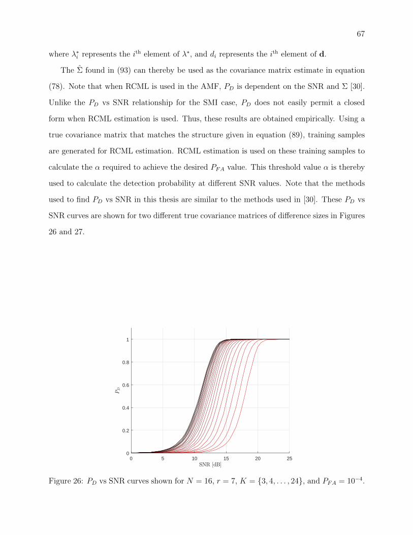
67
where λ∗i represents the ith element of λ∗, and di represents the ith element of d.
The Σ found in (93) can thereby be used as the covariance matrix estimate in equation
(78). Note that when RCML is used in the AMF, PD is dependent on the SNR and Σ [30].
Unlike the PD vs SNR relationship for the SMI case, PD does not easily permit a closed
form when RCML estimation is used. Thus, these results are obtained empirically. Using a
true covariance matrix that matches the structure given in equation (89), training samples
are generated for RCML estimation. RCML estimation is used on these training samples to
calculate the α required to achieve the desired PFA value. This threshold value α is thereby
used to calculate the detection probability at different SNR values. Note that the methods
used to find PD vs SNR in this thesis are similar to the methods used in [30]. These PD vs
SNR curves are shown for two different true covariance matrices of difference sizes in Figures
26 and 27.
0 5 10 15 20 250
0.2
0.4
0.6
0.8
1
Figure 26: PD vs SNR curves shown for N = 16, r = 7, K = {3, 4, . . . , 24}, and PFA = 10−4.

68
0 5 10 15 20 250
0.2
0.4
0.6
0.8
1
Figure 27: PD vs SNR curves shown for N = 24,r = 9, K = {3, 4, . . . , 24}, and PFA = 10−4.
5.2.3 Additional SNR required for clairvoyant performance
The PD vs SNR curves serve as a means of comparing the relative performance between
detectors. However, when PFA and SNR are held constant, it is well known that PD has a
theoretic upper bound [30], characterized by the PD of the clairvoyant detector given in (76).
In general, as K increases, the PD vs SNR curves approach that of the clairvoyant detector,
as shown in Figure 28 below:
Note that the clairvoyant detector is able to achieve any PD value at a lower SNR than
the AMF detectors are able. In other words, some additional amount of SNR is required
for the AMF detectors to reach clairvoyant performance. This can also be thought of as an
”SNR loss”, due to the fact that K training samples are used for AMF detection since the
covariance matrix is unknown. Note that this loss is shown to decrease as K increases.
Reference [40] analyzes this SNR loss for a different, but similar multidimensional CFAR
detector known as the generalized likelihood ratio test (GLRT) detector. In this reference,
Kelly states that this SNR loss is partly due to effective loss factor term ρ (described in
Section A.0.1), and partly due to other losses. Thus, note that the ”SNR loss” described

69
0 5 10 15 20 25SNR [dB]
0
0.2
0.4
0.6
0.8
1
PD
N = 5
0 5 10 15 20 25SNR [dB]
0
0.2
0.4
0.6
0.8
1
PD
N = 15
Figure 28: PD vs SNR for PFA = 10−4 and K = {N, . . . , 200}, shown for different N values.Note that darker curves represent PD values of larger K values.
in this section refers to the additional SNR required for the AMF to reach clairvoyant
performance, and not the ρ term described in Section A.0.1.
Note that this SNR loss term can be found using the formulations for PD of the clairvoyant
detector and AMF, given in (76) and (88) respectively. Using these equations, the PD is fixed
to some value, and the SNR that achieves this PD is obtained for both detectors. Finally,
the ratio between these SNRs yields the SNR loss (the SNR values are subtracted if units
are in decibels).
Note, however, that equations (76) and (88) do not easily permit a closed form for the
SNR. Thus, line search methods (along with the numerical methods required to calculate
(76) and (88)) are used to solve for the SNR loss. These results are shown in Figure 29
below. Clearly, as K increases, the SNR loss approaches 0 dB. Furthermore, the rate at
which the SNR converges differs depends on what N value is being used.
When RCML estimation is used, a simple interpolation method is used to obtain the
SNR loss, since PD does not easily permit a closed form. The SNR loss is taken at PD = 0.6,
since the PD vs SNR curves appear to be linear in this region, as shown in Figure 26 and 27.
Linear interpolation is used in this region to approximate the SNR at which PD = 0.6 for

70
the RCML detector. The ratio between this SNR and the clairvoyant SNR is taken, yielding
the SNR loss. Figure 30 shows the SNR loss as a function of K for two RCML detectors.
Clearly, the SNR loss is dependent on what N and r values are being used.
0 20 40 60 80 100 120 140 160 180 200K
0
5
10
15
20
25
30
35
40
45SNR
loss
[dB]
N = 5N = 10N = 15N = 20N = 25N = 30
Figure 29: SNR loss for AMFs of different N values, shown as a function of K.
0 5 10 15 20 251
2
3
4
5
6
7
8
9
10
Figure 30: SNR loss for RCML AMFs of different N and r values, shown as a function ofK.

71
5.3 Information Elasticity Framework for the AMF
To summarize the previous analysis, it is clear that as the number of secondary samples,
K, increases, the PD of a detector at a given SNR improves up to an asymptotic limit.
The convergence of performance towards this limit can be characterized by the SNR loss, as
shown in Figure 29. However, all of the analysis used to find the SNR loss is based on the
assumption that the K secondary samples are all independent and identically distributed as
disturbance only (thus, homogeneous).
As discussed in Chapter 4, the radar data used as secondary samples are often non-
homogeneous, due to the interference environment and other system factors. Furthermore,
the detection performance has been shown to degrade significantly as a result of using non-
homogeneous training data [21]. Thus, a DM’s selection of K is often restricted or con-
strained based on how many homogeneous training samples are available in a given environ-
ment.
Thus, the choice of K should not solely be based on reducing the SNR loss, but it should
also be based on avoiding the use of non-homogeneous training samples. In general, the
likelihood that the secondary samples contain non-homogeneities increases as K increases [9,
31]. Thus, a trade-off behavior is observed between these two factors. Using the information
elasticity framework, a DM can weigh the cost and benefit of using different K.
Note that the DM also selects a desired PFA value for the AMF, which in turn determines
what the threshold α is set to. Thus, this desired PFA value also affects the PD and the
SNR loss, by virtue of α. In general, as PFA increases, the SNR loss decreases. However,
increasing the PFA is also more costly for a DM, since it increases the number of false alarms.
Thus, the selection of the desired PFA also exhibits a trade-off behavior.
In this particular application, the information quantity parameter is represented by a
vector of length 2: Q = {PFA, K}. K clearly represents the quantity of training data samples
being used to estimate the disturbance covariance matrix. PFA on the other, represents a
probability rather than a quantitative value. However, the desired PFA is directly related to

72
the quantity of false alarms per unit time [9]. The decision quality metric is defined to be the
SNR loss, since it characterizes the relative performance of the detector being considered.
Furthermore, the SNR loss is a function of both PFA and K, and is thus represented as
D(Q).
The constraint function C(Q), on the other hand, is defined to be a function describing
the relative cost of using a particular decision Q. As discussed, a larger K is associated
with a higher likelihood of non-homogeneities, and a larger PFA is associated with more
false alarms. Thus, C(Q) is defined such that an increase in either parameter produces
an increase in C(Q). Furthermore, these constraining factors are highly dependent on the
context, environmental factors, and the preference of the DM. Thus, C(Q) is defined with
user-tunable parameters, allowing a DM to define the relative costs of Q to fit his/her given
application.
Generally, a DM does not consider every possible decision Q. For example, K = 105 is
not a reasonable choice, since it is highly unlikely that 105 homogeneous training samples
are available in any realistic environment. Similarly K = N is not a reasonable choice, since
the SNR loss is unreasonably large for this case. The same logic goes for selecting PFA. For
example, a DM would most likely not select PFA = 0.5, since this would produce far too
many false alarms. Similarly, a DM would not select PFA = 0, since PD = 0 when the PFA
is this low. Given these factors, a DM may choose to select lower and upper bounds of PFA
and K as follows:
a ≤ PFA ≤ b (95)
c ≤ K ≤ d (96)
Note that the selection of these bounds depends on the context and preferences of the DM.
Given decisions in this domain, an approximation for the SNR loss (D(Q)) when SMI is used
is derived in Section 5.3.1. Furthermore, the user-tunable cost function of these decisions
(C(Q) is defined in Section 5.3.2

73
5.3.1 Approximation for SNR loss
The numerical methods used to calculate the SNR loss in Figure 29 are quite computation-
ally expensive and burdensome, especially when having to calculate the SNR loss of many
different decisions. Thus, a closed form approximation for this SNR loss is derived, using
the PD for the Swerling I case. Note that this fluctuation model is considered here because
the equation for PD is much simpler than that of the non-fluctuating case.
From (42) and (85), the AMF detection probability under the Swerling I fluctuation
model is given as follows:
PD =
∫ 1
0
(1 + Aρ
1 + (α + Aρ)
)LK!ρL(1− ρ)N−2
L!(N − 2)!dρ (97)
Furthermore, the clairvoyant detection probability under the Swerling I fluctuation model is
given in (77). Consider the PD conditioned on the random loss factor ρ:
PD|ρ =
(1 + Aρ
1 + (α + A)ρ
)L=
(1ρ
+ A1ρ
+ α + A
)L
(98)
Since the integral in (97) cannot easily be evaluated without using numerical tools, an
approximation is used instead. This approximation is obtained by considering the fact that
the variance of 1/ρ is negligible compared to other terms in (98). This behavior is verified
using Monte Carlo simulations, but is also explained below.
Note that the distribution of ρ is given in (82). Thus, the variance of 1/ρ is derived as
follows:
Var (1/ρ) = E(1/ρ2)− E(1/ρ)2
E(1/ρ2) =
∫ 1
0
1
ρ2
K!ρL(1− ρ)N−2
L!(N − 2)!dρ

74
=K(K − 1)
L(L− 1)
∫ 1
0
(K − 2)!ρL−2(1− ρ)N−2
(L− 2)!(N − 2)!dρ︸ ︷︷ ︸
=1
=K(K − 1)
L(L− 1)
E(1/ρ) =
∫ 1
0
1
ρ
K!ρL(1− ρ)N−2
L!(N − 2)!dρ
=K
L
∫ 1
0
(K − 1)!ρL−1(1− ρ)N−2
(L− 1)!(N − 2)!dρ︸ ︷︷ ︸
=1
=K
L(99)
Var(1/ρ) =K(N − 1)
L2(L− 1)
=m(N − 1)
(m− 1)(N(m− 1) + 1)2(100)
where m is defined to be the ratio m = KN
. Since K > N is necessary for the estimate in
(79) to be non-singular, m must be greater than 1. Consider, PD|ρ ≈ 0 when the SNR is
low, regardless of what value of m is used. Consider the cases when m is near 1, and when
m >> 1.
When m is near 1, we can consider that K is close in value to N . When this is the case,
the PDF of ρ has larger likelihoods at lower ρ values. This causes α to become large, due to
the nature of (87). Intuitively, this is because the threshold term α is affected by the random
loss factor term. As ρ is more likely to be small, the threshold term α should be selected to
be larger to account for this random loss factor. Since α is large, it is generally true that
α >> (1/ρ + A) for low SNR when m is near 1. Thus, PD|ρ ≈ 0. However, as the SNR
increases, α >> (1/ρ+A) will no longer be true, and PD|ρ 6≈ 0. Since α is relatively large in
this case, the SNR at which this occurs is also relatively large. Furthermore, A >> Var(1/ρ)
when the SNR is large enough such that PD|ρ 6≈ 0.

75
Consider also the case when m >> 1. We can consider that K >> N in this case.
Furthermore, since L = K − N + 1, we can also consider L >> 1 in this case. Due to the
size of L, PD|ρ =
(1ρ
+A1ρ
+α+A
)Lwill be approximately 0 for small
1ρ
+A1ρ
+α+A. This is the case
when the SNR is low, i.e. PD|ρ ≈ 0 for low SNR. However, as the SNR increases, eventually
PD|ρ 6≈ 0. Furthermore, when the SNR increases, it is generally true that A >> Var(1/ρ),
since Var(1/ρ) is extremely small when m >> 1, as shown in equation (100).
To summarize the statements made above, the SNR is either low enough such that
PD|ρ ≈ 0, or the SNR is large enough such that A >> Var(1/ρ). Thus, if the variance of 1/ρ
can be thought of as negligible, we can approximate PD by replacing the 1/ρ term in (98)
by its expectation, which is given in (99). Thus:
PD = Eρ(PD|ρ) ≈
E[
1ρ
]+ A
E[
1ρ
]+ α + A
L
PD ≈
(KL
+ AKL
+ α + A
)L
(101)
This approximation shows very close agreement with the PD given in equation (97) calculated
using numerical integration. This close agreement holds for many different PFA, K and N
values, as shown in Figures 31, 32, and 33. Using equations (77) and (101), the SNR loss for
the Swerling I case can be approximated to be:
SNR loss ≈
(α
P1/LD
1− P 1/LD
− K
L
)log(PD)
log(PFAPD
)(102)
Although this approximation was derived using the Swerling I fluctuation model, this ap-
proximation also fits the SNR loss for the nonfluctuating case very closely as well, as shown
in Figure 34.

76
0 10 20 30 40 50 60 70SNR [dB]
0
0.2
0.4
0.6
0.8
1PD
N = 5, PFA = 10−4
PD
PD Approximation
0 10 20 30 40 50 60 70SNR [dB]
0
0.2
0.4
0.6
0.8
1
PD
N = 5, PFA = 10−5
PD
PD Approximation
0 10 20 30 40 50 60 70SNR [dB]
0
0.2
0.4
0.6
0.8
1
PD
N = 5, PFA = 10−6
PD
PD Approximation
Figure 31: Comparison of PD obtained using numerical methods as in (97) and approximationas in (101). PD is shown for N = 5, PFA = {10−4, 10−5, 10−6} values and K = {5, 10, . . . , 50}.

77
0 10 20 30 40 50 60 70SNR [dB]
0
0.2
0.4
0.6
0.8
1PD
N = 50, PFA = 10−4
PD
PD Approximation
0 10 20 30 40 50 60 70SNR [dB]
0
0.2
0.4
0.6
0.8
1
PD
N = 50, PFA = 10−5
PD
PD Approximation
0 10 20 30 40 50 60 70SNR [dB]
0
0.2
0.4
0.6
0.8
1
PD
N = 50, PFA = 10−6
PD
PD Approximation
Figure 32: Comparison of PD obtained using numerical methods as in (97) and approx-imation as in (101). PD is shown for N = 50, PFA = {10−4, 10−5, 10−6} values andK = {50, 51, . . . , 100}.

78
0 10 20 30 40 50 60 70SNR [dB]
0
0.2
0.4
0.6
0.8
1PD
N = 500, PFA = 10−4
PD
PD Approximation
0 10 20 30 40 50 60 70SNR [dB]
0
0.2
0.4
0.6
0.8
1
PD
N = 500, PFA = 10−5
PD
PD Approximation
0 10 20 30 40 50 60 70SNR [dB]
0
0.2
0.4
0.6
0.8
1
PD
N = 500, PFA = 10−6
PD
PD Approximation
Figure 33: Comparison of PD obtained using numerical methods as in (97) and approx-imation as in (101). PD is shown for N = 500, PFA = {10−4, 10−5, 10−6} values andK = {500, 510, . . . , 600}.

79
"approximations fixed".pdf
Figure 34: SNR loss as a function K. Calculations from numerical methods in (97) andapproximation in (102) are displayed together, showing close agreement.
5.3.2 User-defined constraint function
As discussed, the cost function should increase when either K or PFA are increased. Thus,
consider the following functions:
CPFA(PFA) =
(PFA − ab− a
)nfor a ≤ PFA ≤ b (103)
CK(K) =
(K − cd− c
)mfor c ≤ K ≤ d (104)
Consider, equation (103) represents the component of the total cost associated with
using a given PFA, and (104) represents the component of the total cost associated with
using a given K. CPFA(PFA) is defined to increase from 0 to 1, such that CPFA(a) = 0 and
CPFA(b) = 1. Similarly, CK(K) is defined to increase from 0 to 1, such that CK(c) = 0 and
CK(d) = 1. Finally, the n and m parameters allow the DM to change the rate at which these
functions increase.
These functions are defined as such since they are meant to characterize relative cost.

80
Thus a scale is defined over which decisions can be compared, where 1 is defined to be the
maximum cost and 0 is defined to be the minimum cost. With this in mind, the relative cost
of a decision Q is defined as follows:
C(Q) = λ1CPFA(PFA) + λ2CK(K) (105)
for a ≤ PFA ≤ b and c ≤ K ≤ d
s.t. λ1 + λ2 = 1
λ1 and λ2 are defined as weights characterizing the relative importance of CPFA and CK
respectively. Furthermore, λ1 + λ2 = 1 so that the maximum value of C(Q) is still 1. C(Q)
can thus be thought of as a linear combination of the individual cost components CPFA and
CK . Furthermore, C(Q) increases from 0 to 1 as the parameters in Q increase over the
domains defined in (96) and (95), as desired.
5.3.3 AMF decision effectiveness
As with the previous examples of information elasticity, the decision effectiveness E for this
application is dependent on the decision quality metric D(Q) and the constraint function
C(Q). SinceD(Q) and C(Q) are conflicting criteria which the DM wishes to minimize, multi-
objective optimization techniques are used once again to define the decision effectiveness.
For comparison purposes, two constraint functions are shown in Figures 35 and 36, and are
labelled C1(Q) and C2(Q) respectively. Furthermore, a decision quality metric is shown in
Figure 37, labelled D(Q). For sake of clarity, let DM 1 be a decision maker who defines
C1(Q) as their constraint function and D(Q) as their decision quality metric. Similarly, let
DM 2 be a second decision maker who uses C2(Q) as their constraint function and D(Q) as
their decision quality metric.

81
0
0.2
1e-4 60
0.4
0.6C(Q
)
0.8
8e-5 55
1
6e-5
KPFA
504e-5452e-5
1e-6 40
Figure 35: Constraint function C1(Q) for λ1 = λ2 = 0.5, n = m = 1, a = 10−4, b = 10−6,c = 40, and d = 60.
0
0.2
601e-4
0.4
0.6
C(Q
)
0.8
8e-5 55
1
6e-5
PFA K
504e-5452e-5
401e-6
Figure 36: Constraint function C2(Q) for λ1 = 1/3, λ2 = 2/3, n = 2,m = 4, a = 10−4,b = 10−6, c = 40, and d = 60.
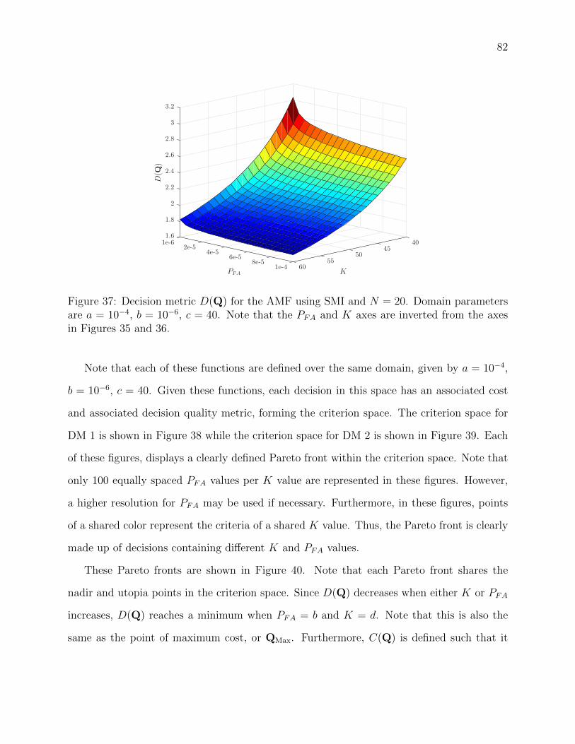
82
1.6
1.8
2
401e-6
2.2
2.4
2.6D(Q
)
2.8
2e-5
3
45
3.2
4e-5
KPFA
506e-5558e-5
601e-4
Figure 37: Decision metric D(Q) for the AMF using SMI and N = 20. Domain parametersare a = 10−4, b = 10−6, c = 40. Note that the PFA and K axes are inverted from the axesin Figures 35 and 36.
Note that each of these functions are defined over the same domain, given by a = 10−4,
b = 10−6, c = 40. Given these functions, each decision in this space has an associated cost
and associated decision quality metric, forming the criterion space. The criterion space for
DM 1 is shown in Figure 38 while the criterion space for DM 2 is shown in Figure 39. Each
of these figures, displays a clearly defined Pareto front within the criterion space. Note that
only 100 equally spaced PFA values per K value are represented in these figures. However,
a higher resolution for PFA may be used if necessary. Furthermore, in these figures, points
of a shared color represent the criteria of a shared K value. Thus, the Pareto front is clearly
made up of decisions containing different K and PFA values.
These Pareto fronts are shown in Figure 40. Note that each Pareto front shares the
nadir and utopia points in the criterion space. Since D(Q) decreases when either K or PFA
increases, D(Q) reaches a minimum when PFA = b and K = d. Note that this is also the
same as the point of maximum cost, or QMax. Furthermore, C(Q) is defined such that it
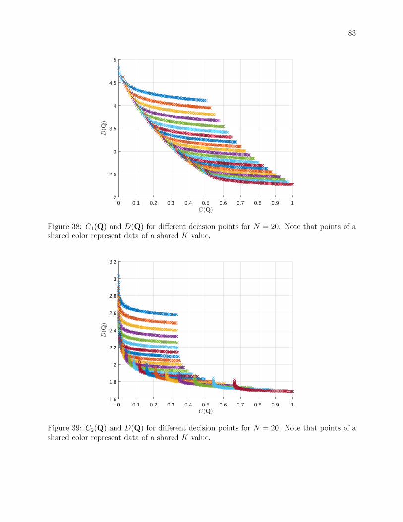
83
0 0.1 0.2 0.3 0.4 0.5 0.6 0.7 0.8 0.9 1C(Q)
2
2.5
3
3.5
4
4.5
5
D(Q
)
Figure 38: C1(Q) and D(Q) for different decision points for N = 20. Note that points of ashared color represent data of a shared K value.
0 0.1 0.2 0.3 0.4 0.5 0.6 0.7 0.8 0.9 1C(Q)
1.6
1.8
2
2.2
2.4
2.6
2.8
3
3.2
D(Q
)
Figure 39: C2(Q) and D(Q) for different decision points for N = 20. Note that points of ashared color represent data of a shared K value.
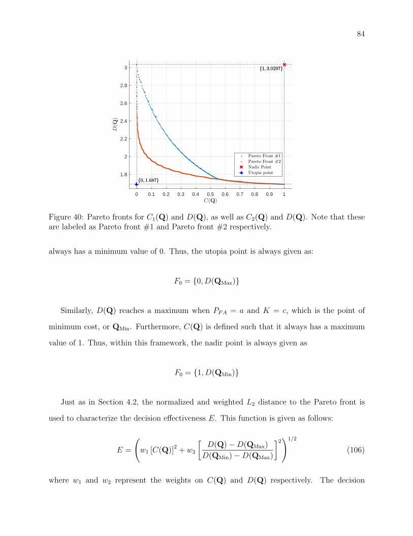
84
0 0.1 0.2 0.3 0.4 0.5 0.6 0.7 0.8 0.9 1C(Q)
1.8
2
2.2
2.4
2.6
2.8
3
D(Q
)
Pareto Front #1Pareto Front #2Nadir PointUtopia point
{0, 1.687}
{1, 3.0297}
{0, 1.687}
{1, 3.0297}
Figure 40: Pareto fronts for C1(Q) and D(Q), as well as C2(Q) and D(Q). Note that theseare labeled as Pareto front #1 and Pareto front #2 respectively.
always has a minimum value of 0. Thus, the utopia point is always given as:
F0 = {0, D(QMax)}
Similarly, D(Q) reaches a maximum when PFA = a and K = c, which is the point of
minimum cost, or QMin. Furthermore, C(Q) is defined such that it always has a maximum
value of 1. Thus, within this framework, the nadir point is always given as
F0 = {1, D(QMin)}
Just as in Section 4.2, the normalized and weighted L2 distance to the Pareto front is
used to characterize the decision effectiveness E. This function is given as follows:
E =
(w1 [C(Q)]2 + w2
[D(Q)−D(QMax)
D(QMin)−D(QMax)
]2)1/2
(106)
where w1 and w2 represent the weights on C(Q) and D(Q) respectively. The decision
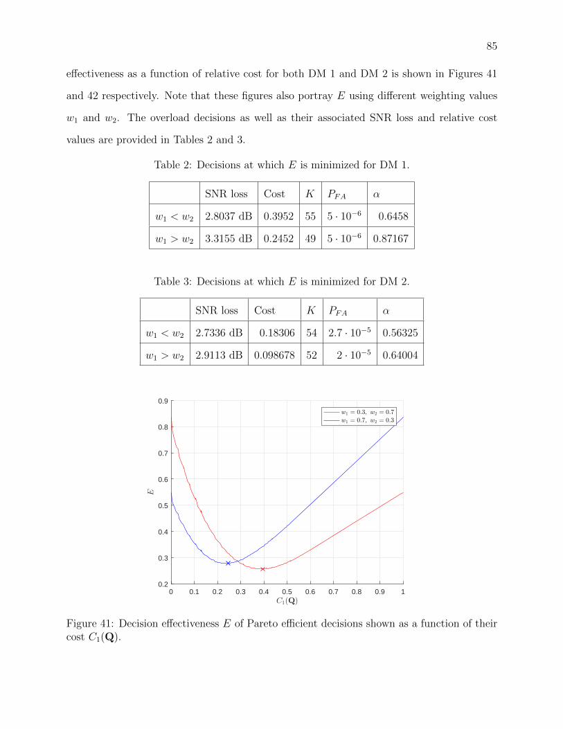
85
effectiveness as a function of relative cost for both DM 1 and DM 2 is shown in Figures 41
and 42 respectively. Note that these figures also portray E using different weighting values
w1 and w2. The overload decisions as well as their associated SNR loss and relative cost
values are provided in Tables 2 and 3.
Table 2: Decisions at which E is minimized for DM 1.
SNR loss Cost K PFA α
w1 < w2 2.8037 dB 0.3952 55 5 · 10−6 0.6458
w1 > w2 3.3155 dB 0.2452 49 5 · 10−6 0.87167
Table 3: Decisions at which E is minimized for DM 2.
SNR loss Cost K PFA α
w1 < w2 2.7336 dB 0.18306 54 2.7 · 10−5 0.56325
w1 > w2 2.9113 dB 0.098678 52 2 · 10−5 0.64004
0 0.1 0.2 0.3 0.4 0.5 0.6 0.7 0.8 0.9 1C1(Q)
0.2
0.3
0.4
0.5
0.6
0.7
0.8
0.9
E
w1 = 0.3, w2 = 0.7
w1 = 0.7, w2 = 0.3
Figure 41: Decision effectiveness E of Pareto efficient decisions shown as a function of theircost C1(Q).
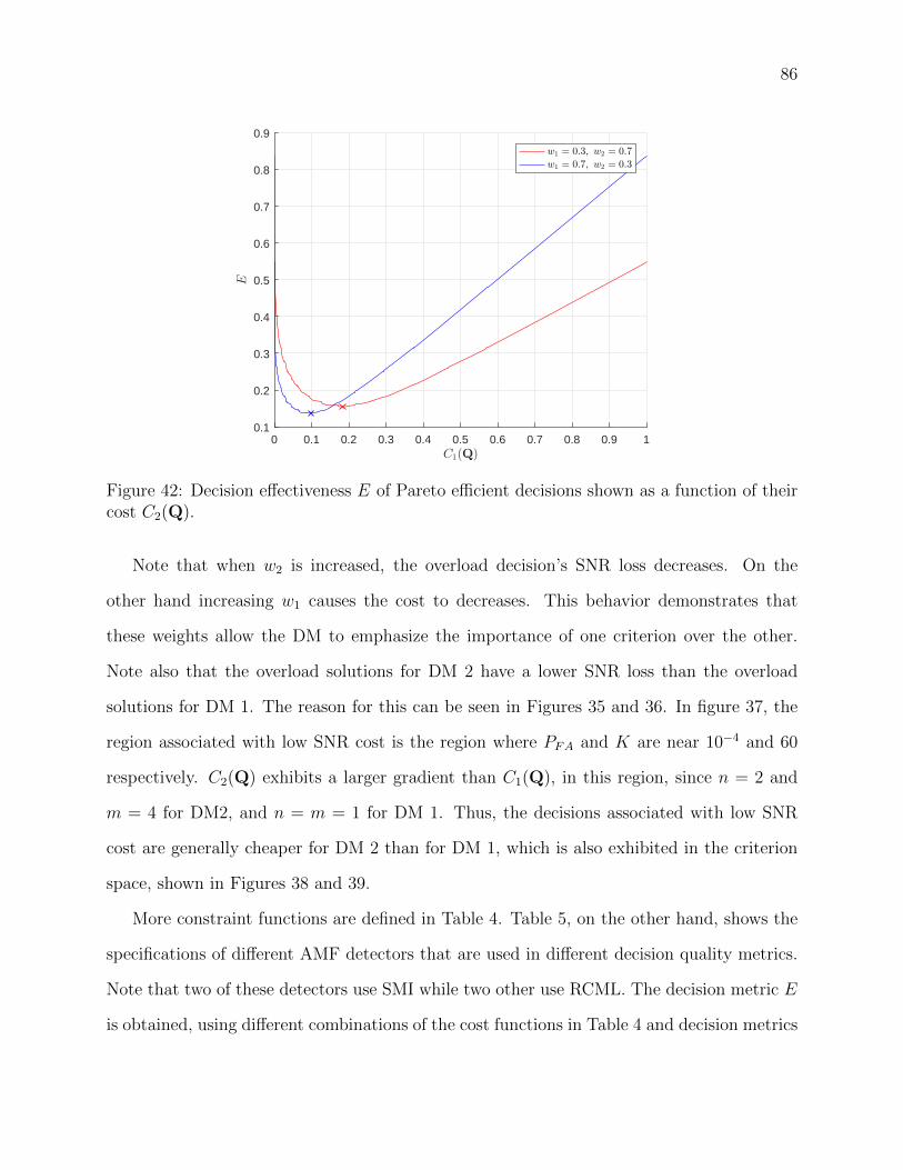
86
0 0.1 0.2 0.3 0.4 0.5 0.6 0.7 0.8 0.9 1C1(Q)
0.1
0.2
0.3
0.4
0.5
0.6
0.7
0.8
0.9
E
w1 = 0.3, w2 = 0.7
w1 = 0.7, w2 = 0.3
Figure 42: Decision effectiveness E of Pareto efficient decisions shown as a function of theircost C2(Q).
Note that when w2 is increased, the overload decision’s SNR loss decreases. On the
other hand increasing w1 causes the cost to decreases. This behavior demonstrates that
these weights allow the DM to emphasize the importance of one criterion over the other.
Note also that the overload solutions for DM 2 have a lower SNR loss than the overload
solutions for DM 1. The reason for this can be seen in Figures 35 and 36. In figure 37, the
region associated with low SNR cost is the region where PFA and K are near 10−4 and 60
respectively. C2(Q) exhibits a larger gradient than C1(Q), in this region, since n = 2 and
m = 4 for DM2, and n = m = 1 for DM 1. Thus, the decisions associated with low SNR
cost are generally cheaper for DM 2 than for DM 1, which is also exhibited in the criterion
space, shown in Figures 38 and 39.
More constraint functions are defined in Table 4. Table 5, on the other hand, shows the
specifications of different AMF detectors that are used in different decision quality metrics.
Note that two of these detectors use SMI while two other use RCML. The decision metric E
is obtained, using different combinations of the cost functions in Table 4 and decision metrics

87
Table 4: Constraint function parameters.
λ1 λ2 n m
Ca(Q) 1/4 3/4 4 2
Cb(Q) 3/4 1/4 4 2
Cc(Q) 1/4 3/4 5 10
Cd(Q) 3/4 1/4 5 10
Ce(Q) 1/4 3/4 15 15
Cf (Q) 3/4 1/4 15 15
Table 5: Specification for decision metrics.
Estimation Type N r a b c dDa(Q) SMI 16 N/A 10−4 10−6 30 40
Db(Q) RCML 16 7 10−4 10−6 10 24
Dc(Q) SMI 24 N/A 10−4 10−6 50 60
Dd(Q) RCML 24 9 10−4 10−6 15 24
in Table 5. The overload solutions for these different combinations are given in Table 6. A
comparison of the associated SNR loss and relative cost values of these overload solutions
are also included in this table.
Clearly, from Table 5, the AMF detectors using RCML use a much smaller domain for K
than the AMF detectors using SMI. In particular, Db(Q) and Dd(Q) only consider K values
up to 24, while Da(Q) considers K values up to 40 and Dc(Q) considers K values up to 60.
The domains are defined as such in order to highlight the fact that RCML estimation is able
to perform well in contexts where the amount of usable training data is scarce.
For example, note that both Da(Q) and Db(Q) are defined for detectors with a dimen-
sionality of 16, but the former considers an SMI detector and the latter considers an RCML
detector. Given the same constraint function Cf (Q), the RCML detector has an overload
solution of K = 23, while the SMI detector has an overload solution of K = 59. Although
the SMI detector selects a much higher value for K, the SNR loss of the RCML detector’s
overload solution is still significantly lower.
Note, however, that there is only one case where the overload solution for an RCML
detector does not outperform the overload solution for an SMI detector. This is when the
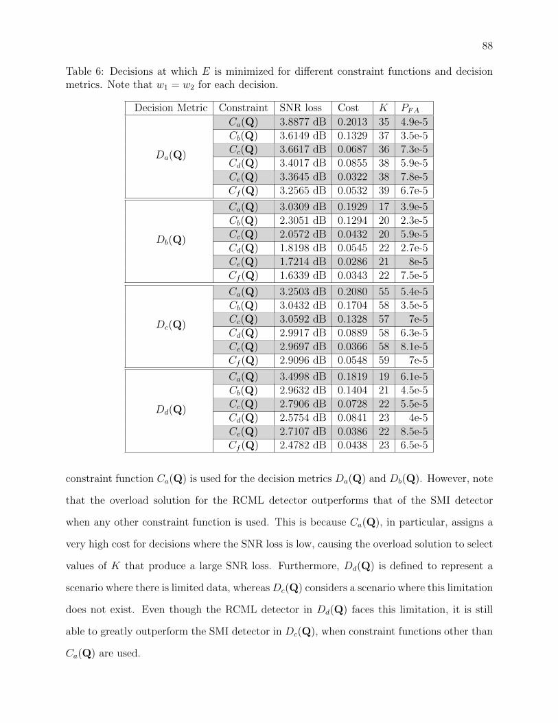
88
Table 6: Decisions at which E is minimized for different constraint functions and decisionmetrics. Note that w1 = w2 for each decision.
Decision Metric Constraint SNR loss Cost K PFA
Da(Q)
Ca(Q) 3.8877 dB 0.2013 35 4.9e-5
Cb(Q) 3.6149 dB 0.1329 37 3.5e-5
Cc(Q) 3.6617 dB 0.0687 36 7.3e-5
Cd(Q) 3.4017 dB 0.0855 38 5.9e-5
Ce(Q) 3.3645 dB 0.0322 38 7.8e-5
Cf (Q) 3.2565 dB 0.0532 39 6.7e-5
Db(Q)
Ca(Q) 3.0309 dB 0.1929 17 3.9e-5
Cb(Q) 2.3051 dB 0.1294 20 2.3e-5
Cc(Q) 2.0572 dB 0.0432 20 5.9e-5
Cd(Q) 1.8198 dB 0.0545 22 2.7e-5
Ce(Q) 1.7214 dB 0.0286 21 8e-5
Cf (Q) 1.6339 dB 0.0343 22 7.5e-5
Dc(Q)
Ca(Q) 3.2503 dB 0.2080 55 5.4e-5
Cb(Q) 3.0432 dB 0.1704 58 3.5e-5
Cc(Q) 3.0592 dB 0.1328 57 7e-5
Cd(Q) 2.9917 dB 0.0889 58 6.3e-5
Ce(Q) 2.9697 dB 0.0366 58 8.1e-5
Cf (Q) 2.9096 dB 0.0548 59 7e-5
Dd(Q)
Ca(Q) 3.4998 dB 0.1819 19 6.1e-5
Cb(Q) 2.9632 dB 0.1404 21 4.5e-5
Cc(Q) 2.7906 dB 0.0728 22 5.5e-5
Cd(Q) 2.5754 dB 0.0841 23 4e-5
Ce(Q) 2.7107 dB 0.0386 22 8.5e-5
Cf (Q) 2.4782 dB 0.0438 23 6.5e-5
constraint function Ca(Q) is used for the decision metrics Da(Q) and Db(Q). However, note
that the overload solution for the RCML detector outperforms that of the SMI detector
when any other constraint function is used. This is because Ca(Q), in particular, assigns a
very high cost for decisions where the SNR loss is low, causing the overload solution to select
values of K that produce a large SNR loss. Furthermore, Dd(Q) is defined to represent a
scenario where there is limited data, whereas Dc(Q) considers a scenario where this limitation
does not exist. Even though the RCML detector in Dd(Q) faces this limitation, it is still
able to greatly outperform the SMI detector in Dc(Q), when constraint functions other than
Ca(Q) are used.

Chapter 6
Conclusion
This thesis covered a framework for making decisions in different applications pertaining
to CFAR detection. This framework is based on the concept of information elasticity, and
sought to characterize the usability properties of different data and processes that provide
information/knowledge to a DM. This usability or decision effectiveness is characterized to
be directly related to different factors that either improve performance (decision quality
metrics) or hinder performance (constraint functions). Through observing how changing
the quantity of information affects these conflicting factors, a point of maximum decision
effectiveness is found and information overload is exhibited.
This framework is applied to an OS-CFAR detector using the FAOSOSD algorithm to
estimate the number of interfering targets present. The accuracy of these estimates at
different SNR levels is analyzed using Monte Carlo simulations. A performance function is
defined by the DM to characterize the relative level of performance of a given decision. Given
the estimated number of interfering targets found via FAOSOSD, the performance function
of many different decisions is found at values of SNR that are relevant to a DM. The sample
mean and variance of the performance function over these different SNR values is taken.
In this decision making scheme, the DM seeks a decision that produces a high average
performance, which represents absolute performance, and a low variance on performance,
89

90
which represents the robustness of a decision. A trade-off behavior between this mean and
variance is exhibited, and compromise programming is used to find the overload solution.
This framework is also applied to the AMF. A domain of usable decisions of K and
desired PFA is defined by a DM. A user-defined function is proposed, which allows the DM
to specify the relative cost of using these decisions. The additional SNR required for the
AMF to perform as well as the clairvoyant detector is also found for each of the usable
decisions. By observing these decisions in the criterion space, a Pareto front is obtained, and
compromise programming is again used to find the overload solution. This analysis is used
on the AMF for when both SMI and RCML are used for covariance matrix estimation. It
is shown that an RCML detector with the same dimensionality as an SMI detector is able
to obtain an overload solution with a much lower SNR loss, even when the DM specifies the
RCML detector to be in a much more data starved scenario.
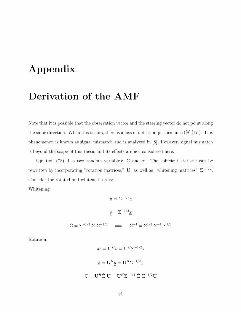
Appendix
Derivation of the AMF
Note that it is possible that the observation vector and the steering vector do not point along
the same direction. When this occurs, there is a loss in detection performance ([8],[17]). This
phenomenon is known as signal mismatch and is analyzed in [8]. However, signal mismatch
is beyond the scope of this thesis and its effects are not considered here.
Equation (78), has two random variables: Σ and x. The sufficient statistic can be
rewritten by incorporating ”rotation matrices,” U, as well as ”whitening matrices” Σ−1/2.
Consider the rotated and whitened terms:
Whitening:
u = Σ−1/2s
y = Σ−1/2x
Σ = Σ−1/2 Σ Σ−1/2 =⇒ Σ−1 = Σ1/2 Σ−1 Σ1/2
Rotation:
de = UHu = UHΣ−1/2s
z = UHy = UHΣ−1/2x
C = UHΣ U = UHΣ−1/2 Σ Σ−1/2U
91

92
Note that U is selected such that the primary data vector and steering vector are ”ro-
tated” to be in the direction of the first elementary vector: e =
[1 0 · · · 0
]T. Also note
that U is selected such that it is unitary [8] (i.e. UHU = UUH = I). Replacing Σ with the
expression in (79) yields:
C = UHΣ−1/2 1
K
K∑k=1
x(k)x(k)H Σ−1/2U
=1
K
K∑k=1
UHΣ−1/2 x(k)x(k)H Σ−1/2U
=1
K
K∑k=1
z(k)z(k)H
=1
KS
where S =K∑k=1
z(k)z(k)H (107)
Note that because U is unitary, UHU = I. Substituting all of these whitened and rotated
terms into the sufficient statistic (78) yields:
Λ =
∣∣∣sHΣ−1x∣∣∣2
sHΣ−1s
=
∣∣∣sHΣ−1/2U UHΣ1/2 Σ−1 Σ1/2U UHΣ−1/2x∣∣∣2
sHΣ−1/2U UHΣ1/2 Σ−1 Σ1/2U UHΣ−1/2s
=
∣∣deHC−1z∣∣2
deHC−1de=d2∣∣eHC−1z
∣∣2d2 eHC−1e
=
∣∣eHC−1z∣∣2
eHC−1e
=
∣∣eHKS−1z∣∣2
eHKS−1e= K
∣∣eHS−1z∣∣2
eHS−1e
Λ =
∣∣eHS−1z∣∣2
eHS−1e
H1
≶H0
α (108)
where in the last line, the constant K in front is absorbed by the threshold constant α.

93
Note that the mean of z is:
E[z] = E[UHΣ−1/2x]
= UHΣ−1/2E[x]
= aUHΣ−1/2s
The magnitude of this mean can be found as:
|E[z]| =√
E[z]HE[z] =√a2sHΣ−1/2UUHΣ−1/2s
= a√sHΣ−1s
Furthermore, if no signal mismatch is assumed, E[z] must point in the same direction as e
(since x points in the same direction as s). Thus, using the magnitude and the direction of
E[z], the mean of z is as follows:
E[z] =(a√sHΣ−1s
)e (109)
Since the steering vector was rotated in the direction of the first elementary vector (its
only non-zero element is in the first position), the following notation is introduced:
Z =
ZAZB
P = S−1 =
PAA PAB
PBA PBB
=
SAA SAB
SBA SBB
−1
where ZA is a scalar representing the first element of Z, and ZB is a N − 1 length vector
representing the rest of Z. Similarly, PAA is a scalar representing the first element in P, PAB
is a 1× (N − 1) vector, PBA is a (N − 1)× 1 vector, and PBB is a (N − 1)× (N − 1) matrix.

94
Using this notation, the statistic can be rewritten. First, consider the denominator of (108):
eHS−1e =
[1 0
]PAA PAB
PBA PBB
1
0
eHS−1e = PAA
Using Frobenius relations for partitioned matrices, otherwise known as matrix inversion in
block form, PAA is rewritten as follows [41]:
eHS−1e = PAA = (SAA − SABS−1BBSBA)−1 (110)
PBA = −S−1BBSAB(SAA − SABS−1
BBSBA)−1
= −S−1BBSBAPAA
PAB = PHBA
PAB = −PAASABS−1BB (111)
Now, consider the numerator of (108):
eHS−1z =
[1 0
]PAA PAB
PBA PBB
ZAZB
= PAAZA + PABZB
Substituting the result in (111) yields:
eHS−1z = PAAZA − PAASABS−1BBZB
= PAA(ZA − SABS−1BBZB) (112)

95
Using the form of the denominator given in (110) and the form of the numerator given
in (112), the sufficient statistic (108) can be rewritten as:
Λ =
∣∣PAA(ZA − SABS−1BBZB)
∣∣2PAA
=
∣∣ZA − SABS−1BBZB
∣∣2P−1AA
=
∣∣ZA − SABS−1BBZB
∣∣2SAA − SABS−1
BBSBA(113)
Now, the following is defined:
y = ZA − SABS−1BBZB
T = SAA − SABS−1BBSBA
Λ =|y|2
T(114)
A.0.1 Distribution of AMF test statistic
The derivation of the statistical behavior of this test statistic is given in [17], and is again
given here for completeness. Note that from equation (107), S can be thought of as K times
the sample covariance matrix of z. Thus, it’s clear that SAB =∑K
k=1 zA(k)zB(k)H . To find
the distribution of y, it is deconstructed as follows:
y = zA − SABS−1BBzB
= zA −K∑k=1
zA(k)zB(k)HS−1BBzB (115)
y appears to be dependent on the scalars zA and zA(k), as well as the vectors/matrices
zB, zB(k), and S−1BB. To find the distribution of y, the ”B vectors” are first considered to be
96
deterministic or given. After the conditional distribution given these B vectors is found, the
expectation across these B vectors can be used to find the actual distribution. From (109),
it’s clear that zA ∼ CN (a√sHΣ−1s, 1) (the covariance of z is I after whitening, thus variance
of zA is 1). Furthermore, the secondary data matrix is assumed to be interference/noise only,
and is thus distributed as: zA(k) ∼ CN (0, 1).
In (115), y is shown to be a linear combination of Gaussians (when B vectors are given).
Thus, y must also be Gaussian. Its mean and variance can be found to be:
E[y] = E[zA]−K∑k=1
E[zA(k)]zB(k)HS−1BBzB
E[y] = a√sHΣ−1s− 0
Var(y) = Var(zA) +K∑k=1
Var(zA(k)zB(k)HS−1BBzB)
= 1 +K∑k=1
Var (zA(k))∣∣zB(k)HS−1
BBzB∣∣2
= 1 +K∑k=1
zHB S−1BBzB(k)zB(k)HS−1
BBzB
= 1 + zHB S−1BB
K∑k=1
(zB(k)zB(k)H
)S−1BBzB
= 1 + zHB S−1BBzB
Thus, y ∼ CN (a√sHΣ−1s, 1− zHB S−1
BBzB). To simplify the problem, this random variable
is normalized to have unit variance, thus the following variables are introduced:
v = y√ρ (116)
ρ = (1 + zHB S−1BBzB)−1 (117)
Thus the new test statistic is:

97
Λ =
∣∣v/√ρ∣∣2T
=|v|2
Tρ
=⇒ |v|2
T
H1
≶H0
αρ (118)
From this normalization, v ∼ CN (b√ρ√sHΣ−1s, 1). It’s important to note that both the
T and ρ terms are random variables. References [17] and [40] show that T is a chi-squared
random variable with K+1−N complex degrees-of-freedom, and ρ follows a beta distribution
with parameters K + 2−N and N − 1.

Bibliography
[1] T. Gospodarek, “Elasticity of information,” Proc. 14th International Congress of Cy-
bernetics and Systems of WOSC, pp. Wroc law, Poland, 511–520, Sept. 2008.
[2] R. M. Narayanan, A. Z. Liu, P. G. Singerman, and M. Rangaswamy, “Information
elasticity in radar systems,” Electronics Letters, vol. 54, no. 17, pp. 1049–1051, 2018.
[3] R. Narayanan, A. Liu, and M. Rangaswamy, “Information elasticity in pseudorandom
code pulse compression,” p. 14, 05 2018.
[4] A. Z. Liu, R. M. Narayanan, and M. Rangaswamy, “Robust decision making method
for adaptive ordered-statistics CFAR technique using information elasticity,” in Radar
Sensor Technology XXIII (K. I. Ranney and A. Doerry, eds.), vol. 11003, pp. 59 – 67,
International Society for Optics and Photonics, SPIE, 2019.
[5] D. Bougherara, G. Grolleau, and N. Mzoughi, “Is more information always better? an
analysis applied to information-based policies for environmental protection,” 2007.
[6] H. Rohling, “New CFAR-processor based on an ordered statistic,” in International
Radar Conference, pp. 271–275, 1985.
[7] W. L. Melvin, “A stap overview,” IEEE Aerospace and Electronic Systems Magazine,
vol. 19, pp. 19–35, Jan 2004.
98

99
[8] F. C. Robey, D. R. Fuhrmann, E. J. Kelly, and R. Nitzberg, “A cfar adaptive matched
filter detector,” IEEE Transactions on Aerospace and Electronic Systems, vol. 28,
pp. 208–216, Jan 1992.
[9] M. Richards, W. Holm, and J. Scheer, Principles of Modern Radar: Basic Principles.
Electromagnetics and Radar, Institution of Engineering and Technology, 2010.
[10] G. W, Shift Register Sequences: Secure And Limited-access Code Generators, Efficiency
Code Generators, Prescribed Property Generators, Mathematical Models (Third Revised
Edition). World Scientific Publishing Company, 2017.
[11] A. Boehmer, “Binary pulse compression codes,” IEEE Transactions on Information
Theory, vol. 13, pp. 156–167, April 1967.
[12] K. Chang, e-Design: Computer-Aided Engineering Design. Elsevier Science, 2016.
[13] G. O. Odu and O. E. Charles-Owaba, “Review of multi-criteria optimization methods -
theory and applications,” IOSR Journal of Engineering, vol. 3, no. 10, pp. 1–14, 2013.
[14] M. Barkat and P. K. Varshney, “On adaptive cell-averaging CFAR (Constant False-
Alarm Rate) radar signal detection,” tech. rep., Oct. 1987.
[15] K. J. Sangston and K. R. Gerlach, “Coherent detection of radar targets in a non-gaussian
background,” IEEE Transactions on Aerospace and Electronic Systems, vol. 30, pp. 330–
340, April 1994.
[16] A. Papoulis and S. U. Pillai, Probability, Random Variables, and Stochastic Processes.
Boston: McGraw Hill, fourth ed., 2002.
[17] E. J. Kelly, “An adaptive detection algorithm,” IEEE Transactions on Aerospace and
Electronic Systems, vol. AES-22, pp. 115–127, March 1986.
[18] J. H. Curtiss, “On the distribution of the quotient of two chance variables,” The Annals
of Mathematical Statistics, vol. 12, no. 4, pp. 409–421, 1941.
100
[19] E. J. Kelly, “Finite-sum expressions for signal detection probabilities,” NASA
STI/Recon Technical Report N, vol. 81, May 1981.
[20] P. Swerling, “Probability of detection for fluctuating targets,” IRE Transactions on
Information Theory, vol. 6, pp. 269–308, April 1960.
[21] B. Himed and W. L. Melvin, “Analyzing space-time adaptive processors using mea-
sured data,” in Conference Record of the Thirty-First Asilomar Conference on Signals,
Systems and Computers (Cat. No.97CB36136), vol. 1, pp. 930–935 vol.1, Nov 1997.
[22] P. P. Gandhi and S. A. Kassam, “Analysis of cfar processors in nonhomogeneous back-
ground,” IEEE Transactions on Aerospace and Electronic Systems, vol. 24, pp. 427–445,
July 1988.
[23] H. David and H. Nagaraja, Order Statistics. Wiley Series in Probability and Statistics,
Wiley, 2004.
[24] S. Blake, “Os-cfar theory for multiple targets and nonuniform clutter,” IEEE Transac-
tions on Aerospace and Electronic Systems, vol. 24, pp. 785–790, Nov 1988.
[25] B. Magaz, A. Belouchrani, and M. Hamadouche, “Automatic threshold selection in os-
cfar radar detection using information theoretic criteria,” Progress In Electromagnetics
Research B, vol. 30, pp. 157–175, 01 2011.
[26] H. Akaike, Information Theory and an Extension of the Maximum Likelihood Principle,
pp. 199–213. New York, NY: Springer New York, 1998.
[27] J. Rissanen, “Modeling by shortest data description,” Automatica, vol. 14, no. 5, pp. 465
– 471, 1978.
[28] M. Wax and T. Kailath, “Detection of signals by information theoretic criteria,” IEEE
Transactions on Acoustics, Speech, and Signal Processing, vol. 33, pp. 387–392, April
1985.
101
[29] Y. Jin and B. Sendhoff, “Trade-off between performance and robustness: An evolu-
tionary multiobjective approach,” in Evolutionary Multi-Criterion Optimization (C. M.
Fonseca, P. J. Fleming, E. Zitzler, L. Thiele, and K. Deb, eds.), (Berlin, Heidelberg),
pp. 237–251, Springer Berlin Heidelberg, 2003.
[30] B. Kang, V. Monga, and M. Rangaswamy, “On the practical merits of rank con-
strained ml estimator of structured covariance matrices,” in 2013 IEEE Radar Con-
ference (RadarCon13), pp. 1–6, April 2013.
[31] M. Weiss, “Analysis of some modified cell-averaging cfar processors in multiple-target
situations,” IEEE Transactions on Aerospace and Electronic Systems, vol. AES-18,
pp. 102–114, Jan 1982.
[32] I. S. Reed, J. D. Mallett, and L. E. Brennan, “Rapid convergence rate in adaptive
arrays,” IEEE Transactions on Aerospace and Electronic Systems, vol. AES-10, pp. 853–
863, Nov 1974.
[33] N. R. Goodman, “Statistical analysis based on a certain multivariate complex gaussian
distribution (an introduction),” Ann. Math. Statist., vol. 34, pp. 152–177, 03 1963.
[34] F. Gini and M. Rangaswamy, Knowledge Based Radar Detection, Tracking and Clas-
sification (Adaptive and Learning Systems for Signal Processing, Communications and
Control Series). New York, NY, USA: Wiley-Interscience, 2008.
[35] M. Steiner and K. Gerlach, “Fast converging adaptive processor or a structured co-
variance matrix,” IEEE Transactions on Aerospace and Electronic Systems, vol. 36,
pp. 1115–1126, Oct 2000.
[36] B. Kang, V. Monga, and M. Rangaswamy, “Rank-constrained maximum likelihood
estimation of structured covariance matrices,” IEEE Transactions on Aerospace and
Electronic Systems, vol. 50, pp. 501–515, January 2014.

102
[37] V. Monga and M. Rangaswamy, “Rank constrained ml estimation of structured co-
variance matrices with applications in radar target detection,” in 2012 IEEE Radar
Conference, pp. 0475–0480, May 2012.
[38] J. Ward, “Space-time adaptive processing for airborne radar,” tech. rep., Massachusettes
Institute of Technology, 12 1994.
[39] M. Skolnik, Radar Handbook, Third Edition. Electronics electrical engineering, McGraw-
Hill Education, 2008.
[40] E. J. Kelly, “Adaptive detection in non-stationary interference, Part III,” Tech. Rep.
761, MIT Lincoln Laboratory, Lexington, MA, Aug. 1987.
[41] E. J. Kelly, “Adaptive detection in non-stationary interference. Part I and Part II,”
Tech. Rep. 724, MIT Lincoln Laboratory, Lexington, MA, May 1985.