
An Important 2-State System: Spin 1/2
59
An Important 2-State System: Spin 1/2 Stern-Gerlach Experiment Energy of magnet in a magnetic field Force on the magnet Watch the animation at http://en.wikipedia.org/wiki/Stern%E2%80%93Gerlach_experiment = − � = − = − � Particles deflection determined by . In other words, the S-G apparatus measures .
Transcript of An Important 2-State System: Spin 1/2

An Important 2-State System: Spin 1/2
Stern-Gerlach Experiment
Energy of magnet in a magnetic field
Force on the magnet
Watch the animation at http://en.wikipedia.org/wiki/Stern%E2%80%93Gerlach_experiment
𝑈𝑈 = −𝛍𝛍 � 𝐁𝐁
𝐹𝐹 = −𝜕𝜕𝑈𝑈𝜕𝜕𝜕𝜕
= −𝛍𝛍 �𝜕𝜕𝐁𝐁𝜕𝜕𝜕𝜕
Particles deflection determined by 𝜇𝜇𝑧𝑧. In other words, the S-G apparatus measures 𝜇𝜇𝑧𝑧.

Sequential Stern-Gerlach (S-G) experiments
https://en.wikipedia.org/wiki/Stern%E2%80%93Gerlach_experiment

To understand the electron and other quantum spins, let’s first look at classical ones –spinning tops
Watch animation at https://en.wikipedia.org/wiki/Top
L
Gθ
⊗ τ
Point mass motion analogy
Rigid body rotation
τ = dL/dt
p = mv L = Iω
F = dp/dtmoment of inertia
Let the distance from spinning top centroid-to-tip distance be l. The torque is τ = lFg sinθ.
dL/dt = ωpLsinθ
⇒ ωp = τ /(Lsinθ) = lFg /L = lFg /(Iω)
The factor lFg /I is determined by the top’s geometry.
ωp ∝ 1/ω
Precession
Exercise: A spinning top’s mass is concentrated in ring of radius R, centered at distance l from the tip. The angular momentum is L = mRv = mR2ω. Using Fg = mg, show that ωp = g(l/R2)/ω.
https://en.wikipedia.org/wiki/Angular_momentum
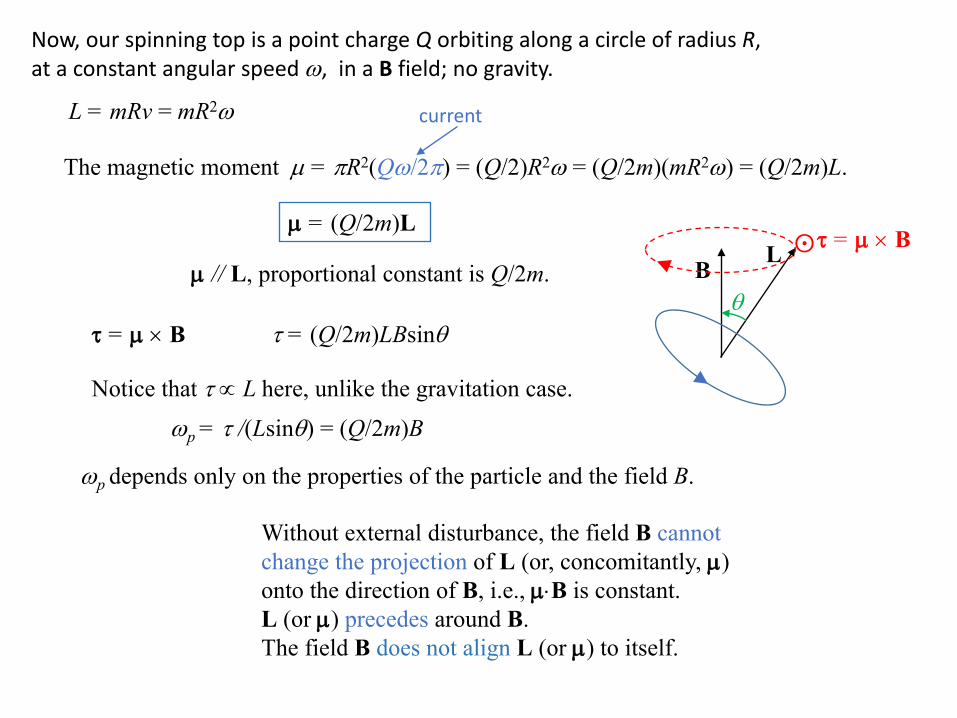
Now, our spinning top is a point charge Q orbiting along a circle of radius R, at a constant angular speed ω, in a B field; no gravity.
L = mRv = mR2ω
The magnetic moment µ = πR2(Qω/2π) = (Q/2)R2ω = (Q/2m)(mR2ω) = (Q/2m)L.
µ = (Q/2m)LL
Bθ
⨀
τ = µ × B
τ = µ × B
τ = (Q/2m)LBsinθ
Notice that τ ∝ L here, unlike the gravitation case.
ωp = τ /(Lsinθ) = (Q/2m)B
ωp depends only on the properties of the particle and the field B.
current
µ // L, proportional constant is Q/2m.
Without external disturbance, the field B cannot change the projection of L (or, concomitantly, µ) onto the direction of B, i.e., µ⋅B is constant. L (or µ) precedes around B. The field B does not align L (or µ) to itself.

current
µ
τ = µ × B ⊗
The free orbiter is very different from the axis-fixed coil in a motor, which would eventually align to Bif the electrical brush was not used.
http://resource.rockyview.ab.ca/rvlc/physics30_BU/Unit_B/m4/p30_m4_l03_p4.html
DC MotorWhy?The coil, as a rigid body, has no angular momentum if not driven by the magnetic field.
For the orbiter, having an angular momentum in the absence of the magnetic field, the torque exerted by the field is “used” to steer the angular momentum.
A turning wheel does not fall, as all bicyclists know.

Quantum mechanics interpretation of the S-G experiment
Spin angular momentum S is intrinsic to the electron. The associated magnetic momentum µ ∝ −S.
The S-G apparatus measures the projection of S in a direction, say the z axis. There can only be two outcomes, +ℏ/2 and −ℏ/2. These are called the two eigenvalues. Each of them corresponds to an eigenstate.
The two states are regarded two orthogonal vectors, labeled |↑⟩ and |↓⟩in Dirac notation. Or, we may label them |0⟩ and |1⟩ in the context of quantum computing.
Not exactly representingA spin state, since the amplitudes are in general complex. (not to be confused with the Bloch Sphere)
|1⟩
|0⟩The electron’s spin state is described by |χ⟩ = 𝑐𝑐↑|↑⟩ + 𝑐𝑐↓|↓⟩, where 𝑐𝑐↑ and 𝑐𝑐↓ are complex numbers, satisfying |𝑐𝑐↑|2 + |𝑐𝑐↓|2 = 1. We just say that |↑⟩ and |↓⟩ form an orthonormal basis set. The electron spin is a 2-state system. Any possible spin state is in the 2D space defined by |↑⟩ and |↓⟩. Therefore, |↑⟩ and |↓⟩ form a complete basis.
In the basis of |↑⟩ and |↓⟩ (or |0⟩ and |1⟩),
|↑⟩ = |0⟩ = 10 , |↓⟩ = |1⟩ = 0
1 , and |χ⟩ = 𝑐𝑐↑𝑐𝑐↓ .
An electron spin is a qubit. This is how a qubit is different from a classical bit: The states of a classical bit can only be two points is the 2D state space. The states of a qubit are richer than the blue dashed circle, since the amplitudes are complex (phase matters).
|𝑐𝑐↑|2 and |𝑐𝑐↓|2 are the probabilities of finding the electron in |↑⟩ and |↓⟩, respectively.

A measurement of a physical quantity only results in eigenvalues. That is, any arbitrary state of a quantum system “collapse” to an eigenstate upon measurement. A physical quantity is represented by an operator, which is a matrix in the state space.
Say, a physical quantity is represented by an operator Q, the eigenvalues are 𝑞𝑞0, 𝑞𝑞1, …, 𝑞𝑞𝑛𝑛, …, corresponding to eigenstates |0⟩, |1⟩, …, |n⟩, …, then Q|n⟩ = 𝑞𝑞𝑛𝑛|n⟩.
Confused? The simple 2-state spin make it easy to understand. Here, the physical quantity is the projection of the spin angular momentum on the z axis, represented by operator 𝑺𝑺𝒛𝒛. The eigenvalues are +ℏ/2 and −ℏ/2, corresponding to eigenstates|↑⟩ and |↓⟩.
𝑺𝑺𝒛𝒛|↑⟩ = (+ℏ/2)|↑⟩ and 𝑺𝑺𝒛𝒛|↓⟩ = (−ℏ/2)|↓⟩
Here, we state without explanation that the Pauli matrices for 𝑺𝑺𝒙𝒙 = (ℏ/2)𝝈𝝈𝒙𝒙 and 𝑺𝑺𝒚𝒚 = (ℏ/2)𝝈𝝈𝒚𝒚 are,
respectively, 𝝈𝝈𝒙𝒙 = 0 11 0 and 𝝈𝝈𝒚𝒚 = 0 −𝑖𝑖
𝑖𝑖 0 .
x
z
y⊙In-class exercise: Show that the eigenvalues of 𝑺𝑺𝒙𝒙 (or 𝝈𝝈𝒙𝒙) are indeed +ℏ/2 and −ℏ/2(or +1 and −1), and that the corresponding eigenstates in the basis of |↑⟩ and |↓⟩ are
|⊙⟩ = |𝜕𝜕+⟩ = 12
11 = 1
2(|↑⟩ + |↓⟩) and |⊗⟩ = |𝜕𝜕−⟩ = 1
21−1 = 1
2(|↑⟩ − |↓⟩) .
Given |↑⟩ = |0⟩ = 10 and |↓⟩ = |1⟩ = 0
1 , we get 𝑺𝑺𝒛𝒛 = (ℏ/2) 1 00 −1 = (ℏ/2)𝝈𝝈𝒛𝒛, where we define
Pauli matrix 𝝈𝝈𝒛𝒛 = 1 00 −1 . ⇒ 𝝈𝝈𝒛𝒛|↑⟩ = |↑⟩ and 𝝈𝝈𝒛𝒛|↓⟩ = −|↓⟩, obvious in the matrix form.

x
z
y⊙
Take-home exercise: Show that 𝝈𝝈𝒙𝒙|↑⟩ = |↓⟩ and 𝝈𝝈𝒙𝒙|↓⟩ = |↑⟩. Side note: 𝝈𝝈𝒙𝒙 is the quantum NOT gate.
Important: An overall phase of a state vector has no physical consequences, e.g., |χ⟩ and 𝑒𝑒𝑖𝑖𝜑𝜑|χ⟩represent the same state.
|←⟩ = |𝑦𝑦−⟩ = 12
1−𝑖𝑖 and i|←⟩ = i|𝑦𝑦−⟩ = 1
2i1 represent the same state, whose spin
angular momentum projected onto y axis is −ℏ/2.
Take-home exercise: Show that the eigenvalues of 𝑺𝑺𝒚𝒚 (or 𝝈𝝈𝒚𝒚) are indeed +ℏ/2 and −ℏ/2(or +1 and −1), and that the corresponding eigenstates in the basis of |↑⟩ and |↓⟩ are
|→⟩ = |𝑦𝑦+⟩ = 12
1i = 1
2(|↑⟩ + i|↓⟩) and |←⟩ = |𝑦𝑦−⟩ = 1
21−𝑖𝑖 = 1
2(|↑⟩ − i|↓⟩).
Take-home exercise: From
|→⟩ = |𝑦𝑦+⟩ = 12
1i = 1
2(|↑⟩ + i|↓⟩) and |←⟩ = |𝑦𝑦−⟩ = 1
21−𝑖𝑖 = 1
2(|↑⟩ − i|↓⟩), show
𝝈𝝈𝒙𝒙|→⟩ = i|←⟩ and 𝝈𝝈𝒙𝒙|←⟩ = − i|→⟩ .
Take-home exercise: Show 𝝈𝝈𝒛𝒛|⊙⟩ = |⊗⟩ and 𝝈𝝈𝒛𝒛 |⊗⟩ = |⊙⟩ ; 𝝈𝝈𝒛𝒛|→⟩ = |←⟩ and 𝝈𝝈𝒛𝒛|←⟩ = |→⟩ .
Side note: Pauli matrices 𝝈𝝈𝒙𝒙, 𝝈𝝈𝒚𝒚, and 𝝈𝝈𝒛𝒛 are known as the X (aka NOT), Y, and Z gates in quantum computing.

https://en.wikipedia.org/wiki/Stern%E2%80%93Gerlach_experiment
We now finally “know” enough to explain the sequential S-G experiments
An electron is in a spin state |χ⟩ = 𝑐𝑐↑|↑⟩ + 𝑐𝑐↓|↓⟩, where |𝑐𝑐↑|2 = |𝑐𝑐↓|2 does not necessarily hold. Upon exiting the first S-G (z axis), the electron collapses to |↑⟩ or |↓⟩, with probabilities |𝑐𝑐↑|2 and |𝑐𝑐↓|2, respectively. Although |𝑐𝑐↑|2 = |𝑐𝑐↓|2 does not necessarily hold for individual electrons, equal counts of spin up and spin down measurements are expected if we do not skew the population.
Only the spin-up electrons are allowed to enter the second S-G (z axis), i.e., those are all in |↑⟩. Therefore, the only possible outcome is spin up.
From |⊙⟩ = |𝜕𝜕+⟩ = 12
(|↑⟩ + |↓⟩) and |⊗⟩ = |𝜕𝜕−⟩ = 12
(|↑⟩ − |↓⟩), we have |↑⟩ = 12
(|𝜕𝜕+⟩ + |𝜕𝜕−⟩) and
|↓⟩ = 12
(|𝜕𝜕+⟩ − |𝜕𝜕−⟩). We thus have equal probability of detecting |𝜕𝜕+⟩ and |𝜕𝜕−⟩ for each electron. Exercise: write these expressions in the matrix form in the basis of |↑⟩ and |↓⟩.
This is now obvious from |𝜕𝜕+⟩ = 12
(|↑⟩ + |↓⟩) and |𝜕𝜕−⟩ = 12
(|↑⟩ − |↓⟩). We thus have equal probability of detecting |𝜕𝜕+⟩ and |𝜕𝜕−⟩ for each electron.

Common (or simultaneous) eigenstates
For an electron in |↑⟩, 𝝈𝝈𝒛𝒛|↑⟩ = |↑⟩. From 𝝈𝝈𝒙𝒙|↑⟩ = |↓⟩ = 12
(|𝜕𝜕+⟩ − |𝜕𝜕−⟩), which is neither |𝜕𝜕+⟩ nor |𝜕𝜕−⟩, we see that the eigenstate |↑⟩ of 𝝈𝝈𝒛𝒛 is not an eigenstate of 𝝈𝝈𝒙𝒙. Therefore, 𝑺𝑺𝒛𝒛 and 𝑺𝑺𝒙𝒙 cannot be determined at the same time. 𝑺𝑺𝒛𝒛 and 𝑺𝑺𝒙𝒙 do not have common (or simultaneous) eigenstates.
Since 𝝈𝝈𝒛𝒛|↑⟩ = |↑⟩, we can write 𝝈𝝈𝒙𝒙|↑⟩ = |↓⟩ = 𝝈𝝈𝒙𝒙 (𝝈𝝈𝒛𝒛|↑⟩) = (𝝈𝝈𝒙𝒙 𝝈𝝈𝒛𝒛)|↑⟩, therefore 𝝈𝝈𝒙𝒙 𝝈𝝈𝒛𝒛|↑⟩ = |↓⟩.On the other hand, 𝝈𝝈𝒛𝒛 𝝈𝝈𝒙𝒙|↑⟩ = 𝝈𝝈𝒛𝒛 (𝝈𝝈𝒙𝒙 |↑⟩) = 𝝈𝝈𝒛𝒛 |↓⟩ = −|↓⟩.
Apparently, 𝝈𝝈𝒙𝒙 𝝈𝝈𝒛𝒛 ≠ 𝝈𝝈𝒛𝒛 𝝈𝝈𝒙𝒙. It appears that 𝝈𝝈𝒙𝒙 𝝈𝝈𝒛𝒛 = − 𝝈𝝈𝒛𝒛 𝝈𝝈𝒙𝒙.
In-class exercise: Use matrix multiplication to show 𝝈𝝈𝒙𝒙 𝝈𝝈𝒛𝒛 = − 𝝈𝝈𝒛𝒛 𝝈𝝈𝒙𝒙 is generally true.

Solution: Applying matrix multiplication to matrices 𝝈𝝈𝒙𝒙 and 𝝈𝝈𝒛𝒛, we get 𝝈𝝈𝒙𝒙 𝝈𝝈𝒛𝒛 = 0 −11 0 and
𝝈𝝈𝒛𝒛 𝝈𝝈𝒙𝒙= 0 1−1 0 . Therefore 𝝈𝝈𝒙𝒙 𝝈𝝈𝒛𝒛 = − 𝝈𝝈𝒛𝒛 𝝈𝝈𝒙𝒙 .
The Pauli matrices do not commute with each other. Operators that do not commute do not have simultaneous eigenstates (obviously).
Take-home exercise: Use matrix multiplication to show 𝝈𝝈𝒙𝒙𝟐𝟐 = 𝝈𝝈𝒚𝒚𝟐𝟐 = 𝝈𝝈𝒛𝒛𝟐𝟐 = 1 00 1 = I. The unit
matrix I can be written as simply 1.
𝝈𝝈𝒙𝒙𝟐𝟐 = 𝝈𝝈𝒚𝒚𝟐𝟐 = 𝝈𝝈𝒛𝒛𝟐𝟐 = 1 00 1 = I ⇒ 𝑺𝑺𝒙𝒙𝟐𝟐 = 𝑺𝑺𝒚𝒚𝟐𝟐 = 𝑺𝑺𝒛𝒛𝟐𝟐 = ℏ2/4
Homework 2: Problem 1. (a) Find the eigenvalues and the corresponding eigenstates of 𝝈𝝈𝒙𝒙 𝝈𝝈𝒛𝒛. (b) Find the eigenvalues and the corresponding eigenstates of 𝝈𝝈𝒛𝒛 𝝈𝝈𝒙𝒙. (c) Compare your results with the eigenvalues and the corresponding eigenstates of 𝝈𝝈𝒚𝒚. Explain your observations.
Problem 2. Find a relation between 𝝈𝝈𝒚𝒚 and 𝝈𝝈𝒛𝒛, which is similar to 𝝈𝝈𝒙𝒙 𝝈𝝈𝒛𝒛 = − 𝝈𝝈𝒛𝒛 𝝈𝝈𝒙𝒙.
While 𝑺𝑺𝒛𝒛, 𝑺𝑺𝒙𝒙, and 𝑺𝑺𝒚𝒚 cannot be determined at the same time, 𝑺𝑺𝒙𝒙𝟐𝟐 = 𝑺𝑺𝒚𝒚𝟐𝟐 = 𝑺𝑺𝒛𝒛𝟐𝟐 = ℏ2/4 always holds, i.e., they are always determined and 𝑺𝑺𝒙𝒙𝟐𝟐, 𝑺𝑺𝒚𝒚𝟐𝟐, and 𝑺𝑺𝒛𝒛𝟐𝟐 all have simultaneous eigenstates with each of 𝑺𝑺𝒙𝒙, 𝑺𝑺𝒚𝒚, and 𝑺𝑺𝒛𝒛.

𝝈𝝈𝒙𝒙𝟐𝟐 = 𝝈𝝈𝒚𝒚𝟐𝟐 = 𝝈𝝈𝒛𝒛𝟐𝟐 = 1 00 1 = I ⇒ 𝑺𝑺𝒙𝒙𝟐𝟐 = 𝑺𝑺𝒚𝒚𝟐𝟐 = 𝑺𝑺𝒛𝒛𝟐𝟐 = ℏ2/4
For 𝑺𝑺𝒛𝒛 = ±ℏ/2 (i.e. 𝝈𝝈𝒛𝒛 = ±1), we have 𝑺𝑺𝒙𝒙𝟐𝟐 = 𝑺𝑺𝒚𝒚𝟐𝟐 = 𝑺𝑺𝒛𝒛𝟐𝟐 = ℏ2/4 for both ↑⟩ and |↑⟩. It is said that ↑⟩ and |↑⟩are degenerate in each of 𝑺𝑺𝒙𝒙𝟐𝟐, 𝑺𝑺𝒚𝒚𝟐𝟐, and 𝑺𝑺𝒛𝒛𝟐𝟐. Similarly, |⊙⟩ and |⊗⟩ are degenerate in each of these quantities. So are |→⟩ and |←⟩.
Relations between operators in quantum mechanics follow those between physical quantities known in classical physics.
Therefore, the total spin angular momentum 𝑺𝑺2 = 𝑺𝑺𝒙𝒙𝟐𝟐 + 𝑺𝑺𝒚𝒚𝟐𝟐 + 𝑺𝑺𝒛𝒛𝟐𝟐 = 3ℏ2/4. This can be loosely interpreted as the magnitude of the total spin angular momentum is always
S = |S| = 32ℏ. Finally, the picture of spin emerges:
z
y⊙xℏ/2
ℏ/2
In an applied DC magnetic field B = −𝐵𝐵�𝐳𝐳, |↑⟩ and |↓⟩ are the low- and high-energy states, respectively. But, the field B itself does not align them; they can be considered as preceding around B. In the presence of disturbance from the environment(sometimes called the bath), an electron does not stay in a definitive state for long. At sufficiently low temperatures and after sufficiently long time, all electrons will be in the low-energy state |↑⟩.
B

More about Dirac notationThe ket |χ⟩ denotes a state independent of our choice of the basis. |χ⟩ = 𝑐𝑐⊙|⊙⟩ + 𝑐𝑐⊗|⊗⟩ = 𝑐𝑐→|→⟩ + 𝑐𝑐←|←⟩ = 𝑐𝑐↑|↑⟩ + 𝑐𝑐↓|↓⟩
Take-home exercise: Find ⟨↑|⊙⟩ and ⟨↑|⊗⟩, and think about the sequential S-G measurements 𝝈𝝈𝒙𝒙 𝝈𝝈𝒛𝒛again.
In the basis of |↑⟩ and |↓⟩ (or |0⟩ and |1⟩), |χ⟩ = 𝑐𝑐↑𝑐𝑐↓ .
We now define the bra ⟨χ| = 𝑐𝑐↑∗ 𝑐𝑐↓
∗ . Obviously ⟨χ|χ⟩ = 1. The state vector is normalized.
The basis of |↑⟩ and |↓⟩ (or |0⟩ and |1⟩) is said to be orthonormal because ⟨↑|↑⟩ = 1, ⟨↓|↓⟩ = 1, and ⟨↑|↓⟩ = 0.
Similarly, the same is said of the basis set |⊙⟩ and |⊗⟩ and the basis set |→⟩ and |←⟩ .
Recall that the inner product ⟨a|b⟩ is the projection of |b⟩ on to |a⟩. When project a vector onto a basis vector, you get the amplitude:For arbitrary |χ⟩ = 𝑐𝑐↑|↑⟩ + 𝑐𝑐↓|↓⟩, we have ⟨↑|χ⟩ = 𝑐𝑐↑ and ⟨↓|χ⟩ = 𝑐𝑐↓.
Notice that the elements of the bra are complex conjugates of the corresponding ones in the ket.
⟨a|b⟩ = 𝑎𝑎0∗ 𝑎𝑎1∗𝑏𝑏0𝑏𝑏1
= 𝑎𝑎0∗𝑏𝑏0 + 𝑎𝑎1∗𝑏𝑏1 is the inner product of the two vectors |a⟩ = 𝑎𝑎0𝑎𝑎1 and |b⟩ = 𝑏𝑏0𝑏𝑏1
.

Energy and time evolution of a quantum systemFor a physical quantity Q represented by an operator Q, with eigenvalues 𝑞𝑞0, 𝑞𝑞1, 𝑞𝑞2, …, 𝑞𝑞𝑛𝑛, …, corresponding to eigenstates |0⟩, |1⟩, …, |n⟩, …, we have Q|n⟩ = 𝑞𝑞𝑛𝑛|n⟩.
In the basis of |0⟩, |1⟩, …, |n⟩, …, the matrix Q is diagonalized. This is obvious in the matrix form.
Energy E is such a special quantity that we give its operator a special name, the Hamiltonian H, with eigenvalues 𝐸𝐸0, 𝐸𝐸1, 𝐸𝐸2, …, 𝐸𝐸𝑛𝑛, …, corresponding to eigenstates |0⟩, |1⟩, …, |n⟩, … We have H|n⟩ = 𝐸𝐸𝑛𝑛|n⟩.
An energy eigenstate (i.e. a state with a definitive energy), |n⟩, evolves in time following
|n(t)⟩ = 𝑒𝑒−𝑖𝑖𝐸𝐸𝑛𝑛ℏ 𝑡𝑡 |n(0)⟩ = 𝑒𝑒−𝑖𝑖𝜔𝜔𝑛𝑛𝑡𝑡 |n(0)⟩, where 𝜔𝜔𝑛𝑛 = 𝐸𝐸𝑛𝑛/ℏ.
For a system in an energy eigenstate (i.e. a state with a definitive energy), |n⟩, this phase evolution has no observable physical consequences.
For a system in a state that is a linear combination of energy eigenstates, |ψ⟩ = ∑𝑛𝑛 𝑐𝑐𝑛𝑛|n⟩, each frequency evolves at a different frequency and beating happens.
This idea can be expressed in the matrix form, |ψ (t)⟩ = U(t) |ψ (0)⟩, where U(t) is a diagonalizedmatrix with the nth diagonal element being 𝑒𝑒−𝑖𝑖𝜔𝜔𝑛𝑛𝑡𝑡.
Too abstract? Let’s make it clear with a simple 2-state system example:Consider an electron in a DC magnetic field B in the −z direction. Recall that the energy is −µ⋅B. Since the magnetic moment µ ∝ −S, the energy ∝ −𝑆𝑆𝑧𝑧B. Therefore, 𝑺𝑺𝒛𝒛 and H have common eigenstates. For conformation to the quantum computing notations, and for extension to other 2-state systems, we now label the up- and down-spin states |0⟩ and |1⟩. We then have H|0⟩ = ℏ𝜔𝜔0|0⟩ and H|1⟩ = ℏ𝜔𝜔1|1⟩

For an electron in a DC magnetic field, the up- and down-spin states, labeled |0⟩ and |1⟩, we have H|0⟩ = ℏ𝜔𝜔0|0⟩ and H|1⟩ = ℏ𝜔𝜔1|1⟩
|0(t)⟩ = 𝑒𝑒−𝑖𝑖𝜔𝜔0𝑡𝑡 |0(0)⟩ ≡ 𝑒𝑒−𝑖𝑖𝜔𝜔0𝑡𝑡 |0⟩|1(t)⟩ = 𝑒𝑒−𝑖𝑖𝜔𝜔1𝑡𝑡 |1(0)⟩ ≡ 𝑒𝑒−𝑖𝑖𝜔𝜔1𝑡𝑡 |1⟩
The electron was initially in the state |⊙⟩ = |𝜕𝜕+⟩ = 12
(|↑⟩ + |↓⟩) at t = 0. Since B // −z, it is not an
eigenstate of H. We now label it as |+⟩ = 12
(|0⟩ + |1⟩). Let’s follow the time evolution of this electron:
|χ(t)⟩ = 12
(𝑒𝑒−𝑖𝑖𝜔𝜔0𝑡𝑡 |0⟩ + 𝑒𝑒−𝑖𝑖𝜔𝜔1𝑡𝑡 |1⟩)
Let ω = 𝜔𝜔1 − 𝜔𝜔0, and we have |χ(t)⟩ = 12𝑒𝑒−𝑖𝑖
𝜔𝜔0+𝜔𝜔12 𝑡𝑡 (𝑒𝑒𝑖𝑖
𝜔𝜔2𝑡𝑡|0⟩ + 𝑒𝑒−𝑖𝑖
𝜔𝜔2𝑡𝑡|1⟩).
Inserting |0⟩ = 12
(|+⟩ + |−⟩) and |1⟩ = 12
(|+⟩ − |−⟩) leads to
|χ(t)⟩ = 12𝑒𝑒−𝑖𝑖
𝜔𝜔0+𝜔𝜔12 𝑡𝑡 [(𝑒𝑒𝑖𝑖
𝜔𝜔2𝑡𝑡 + 𝑒𝑒−𝑖𝑖
𝜔𝜔2𝑡𝑡)|+⟩ + (𝑒𝑒𝑖𝑖
𝜔𝜔2𝑡𝑡 − 𝑒𝑒−𝑖𝑖
𝜔𝜔2𝑡𝑡)|−⟩]
= 𝑒𝑒−𝑖𝑖𝜔𝜔0+𝜔𝜔1
2 𝑡𝑡 [(cos𝜔𝜔2𝑡𝑡)|+⟩ + (sin𝜔𝜔
2𝑡𝑡)|−⟩].
These are real amplitudes with observable physical consequences!
Overall phase with no observable physical consequences.
If we measure electron spin in z-direction at time t, what are the probabilities of getting +ℏ/2 and −ℏ/2?If we measure electron spin in x-direction at time t, what are the probabilities of getting +ℏ/2 and −ℏ/2?
Questions:

In this case where |+⟩ = 12
(|0⟩ + |1⟩) at t = 0, it is said that the system is prepared in an initial state |+⟩. Since B // −z, it is not an eigenstate of H, i.e., the system does not have a definitive energy. The prepared initial state is a superposition of the high- and low-energy states (or spin-up and -down states).In such cases, beating happens.
Questions:If the system is prepared in an initial state |0⟩, everything else the same as in the above case, how do the probabilities of measuring spin up and spin down change with time?Will there be beating between |0⟩ and |1⟩?
Answers:The probabilities of measuring spin up and spin down will remain 1 and 0, respectively.There is no beating between |0⟩ and |1⟩.
The reason is that |0⟩ is an eigenstate of H, i.e., with a definitive energy, and therefore a definitive rate of phase evolution, 𝜔𝜔0.Therefore, an energy eigenstate is said to be a stationary state.
Will the electron remain in |0⟩ forever?Yes and No. If H ∝ −B𝑆𝑆𝑧𝑧 indeed, without any other contributions, then yes. But, quantum computing would be too easy if this were the case. There will always be disturbance from the environment, which add to the Hamiltonian.

Potential energy
The chemical bond of H2+ is
also a 2-state systemThe electron is shared by the two protons, resulting in two stationary states:
|L⟩: the electron associated with the left H atom
|R⟩: the electron associated with the right H atom
Bonding: |0⟩ = 12
(|L⟩ + |R⟩) and
Antibonding: |1⟩ = 12
(|L⟩ − |R⟩)

The chemical bond of H2+ is also a 2-state system
The electron is shared by the two protons, resulting in two stationary states:
|L⟩: the electron associated with the left H atom
|R⟩: the electron associated with the right H atom
Bonding: |0⟩ = 12
(|L⟩ + |R⟩),lower-energy, symmetric
Antibonding: |1⟩ = 12
(|L⟩ − |R⟩), higher-energy, antisymmetric
Questions:If we prepare an H2
+ in an initial state |L⟩ at t = 0 and measure whether the electron is associated with the left or right proton, how do the probabilities of measuring left and right change with time?What if we prepare the H2
+ in |0⟩ at t = 0 ?
Answers:If we prepare an H2
+ in |L⟩ at t = 0 and measure whether the electron is associated with the left or right proton, the probabilities of measuring left and right will oscillate back and forth at the frequency determined by half the energy difference between the bonding (|0⟩) and antibonding (|1⟩) states.What if we prepare the H2
+ in |0⟩ at t = 0, it will stay there forever. The probabilities are half/half for measuring left and right.

For a physical quantity Q represented by an operator Q, with eigenvalues 𝑞𝑞0, 𝑞𝑞1, …, 𝑞𝑞𝑛𝑛, …, corresponding to eigenstates |0⟩, |1⟩, …, |n⟩, …, we have Q|n⟩ = 𝑞𝑞𝑛𝑛|n⟩. This can be written in the matrix form.
Quantities with continuous eigenvalues and Schrödinger equation
If there are N eigenvalues corresponding to N eigenstates, the state space is N-dimensional.
The 2-state systems we discussed are the simplest. N may be infinity for the N-state system.
The spectrum of the eigenvalues may even be continuous!
Let’s now consider the position of a particle in space.For simplicity, let’s say the space is 1-D and the positions is x, which is continuous. (Obviously, aparticle in uniform, free space has equal probability to be at any x.)
Let |x⟩ be the state in which the particle is localized at x.
For an system, an arbitrary state |ψ⟩ = ∑𝑛𝑛 𝑐𝑐𝑛𝑛|n⟩.
Recall that for 2-state systems, an arbitrary state |χ⟩ = 𝑐𝑐0|0⟩ + 𝑐𝑐1|1⟩.
Similarly, for continuous x, an arbitrary state |ψ⟩ = ∫−∞∞ 𝑑𝑑𝜕𝜕ψ 𝜕𝜕 |x⟩.
Here, for continuous x, ψ 𝜕𝜕 is the amplitude of |x⟩ in |ψ⟩, i.e., projection of |ψ⟩ onto |x⟩, just as 𝑐𝑐𝑛𝑛 is to |ψ⟩ = ∑𝑛𝑛 𝑐𝑐𝑛𝑛|n⟩ in the discrete case.
2-state: 𝑐𝑐0 = ⟨0|χ⟩ and 𝑐𝑐1 = ⟨1|χ⟩Discrete: 𝑐𝑐𝑛𝑛 = ⟨𝑛𝑛|ψ⟩
ψ 𝜕𝜕 = ⟨𝜕𝜕|ψ⟩
For continuous xby analogy
Question: What is the physical meaning of |ψ 𝜕𝜕 |2?
From discrete to continuous, summation becomes integral

Answer: Just as |𝑐𝑐𝑛𝑛|2 = |⟨𝑛𝑛|χ⟩|2 is the probability of finding the system in state |n⟩, |ψ 𝜕𝜕 |2 = |⟨𝜕𝜕|ψ⟩|2 is the probability of finding the system in state |x⟩, i.e., at location x.
Obviously, H and p have simultaneous eigenstates. In the 1D case, two momenta ±p correspond to the same energy E, i.e., the two corresponding eigenstates are degenerate in energy.
As for discrete states, the wave function is to be normalized: ∫−∞∞ 𝑑𝑑𝜕𝜕|ψ 𝜕𝜕 |2 = 1 .
Note: Not all wave functions can be normalized this way. We will re-examine normalization later.
Question: What is the physical meaning of |ψ 𝜕𝜕 |2?
Let’s now consider a particle in free space.Potential energy same everywhere, set it to 0. The total energy is the kinetic energy.
Relations between operators in quantum mechanics follow those between the corresponding physical quantities known in classical physics.
Recall the following:
Hamiltonian (energy) H = 𝒑𝒑2
2𝑚𝑚
momentummass
You may have learned that ψ 𝜕𝜕 is the wave function.

Obviously, H and p have simultaneous eigenstates. In the 1D case, two momenta ±p correspond to the same energy E, i.e., the two corresponding eigenstates are degenerate in energy.
Hamiltonian (energy) H = 𝒑𝒑2
2𝑚𝑚
momentummass
p |p⟩ = 𝑝𝑝 |p⟩momentum operator
momentum eigenvalue
momentum eigenstate corresponding to eigenvalue p
Since |p⟩ is an eigenstate of H, |p⟩(t) = 𝑒𝑒−𝑖𝑖𝐸𝐸ℏ𝑡𝑡|p⟩(0) = 𝑒𝑒−𝑖𝑖𝜔𝜔𝑡𝑡 |p⟩(0), where 𝜔𝜔 = 𝐸𝐸
ℏ,
The wave function of |p⟩ is ψ𝑝𝑝 𝜕𝜕 = ⟨𝜕𝜕|p⟩.
|p⟩ = ∫−∞∞ 𝑑𝑑𝜕𝜕ψ𝑝𝑝 𝜕𝜕 |x⟩.
Let’s examine the time evolution of |p⟩(t) = ∫−∞∞ 𝑑𝑑𝜕𝜕ψ𝑝𝑝 𝜕𝜕, 𝑡𝑡 |x⟩.
ψ𝑝𝑝 𝜕𝜕, 𝑡𝑡 =𝑒𝑒−𝑖𝑖𝜔𝜔𝑡𝑡ψ𝑝𝑝 𝜕𝜕, 0 = 𝑒𝑒−𝑖𝑖𝜔𝜔𝑡𝑡ψ𝑝𝑝 𝜕𝜕 .
Classically, the particle moves at a constant speed 𝑣𝑣 = ⁄𝑝𝑝 𝑚𝑚, therefore ψ𝑝𝑝 𝜕𝜕 − 𝑣𝑣𝑡𝑡, 0 = ψ𝑝𝑝 𝜕𝜕, 𝑡𝑡 .
⇒ ψ𝑝𝑝 𝜕𝜕 − 𝑣𝑣𝑡𝑡, 0 = ψ𝑝𝑝 𝜕𝜕 − 𝑣𝑣𝑡𝑡 = 𝑒𝑒−𝑖𝑖𝜔𝜔𝑡𝑡ψ𝑝𝑝 𝜕𝜕 .

ψ𝑝𝑝 𝜕𝜕 − 𝑣𝑣𝑡𝑡, 0 = ψ𝑝𝑝 𝜕𝜕 − 𝑣𝑣𝑡𝑡 = 𝑒𝑒−𝑖𝑖𝜔𝜔𝑡𝑡ψ𝑝𝑝 𝜕𝜕 .
We can immediately see ψ𝑝𝑝 𝜕𝜕, 𝑡𝑡 = 𝑒𝑒−𝑖𝑖𝜔𝜔(𝑡𝑡−𝑥𝑥𝑣𝑣) = 𝑒𝑒𝑖𝑖(𝜔𝜔𝑣𝑣𝑥𝑥−𝜔𝜔𝑡𝑡).
𝜔𝜔𝑣𝑣
= 𝐸𝐸/ℏ⁄𝑝𝑝 𝑚𝑚
= 𝒑𝒑2
2𝑚𝑚ℏ⁄𝑝𝑝 𝑚𝑚
= ⁄𝑝𝑝 ℏ .⇒
ψ𝑝𝑝 𝜕𝜕, 𝑡𝑡 = 𝑒𝑒𝑖𝑖(𝑘𝑘𝑥𝑥−𝜔𝜔𝑡𝑡)
define k = ⁄𝑝𝑝 ℏ
There seems to be an obvious problem: |ψ𝑝𝑝 𝜕𝜕 |2 = 1 and therefore ∫−∞∞ 𝑑𝑑𝜕𝜕|ψ𝑝𝑝 𝜕𝜕 |2 = ∞.
We need to re-examine normalization.
For a physical quantity Q represented by an operator Q, with N discrete eigenvalues 𝑞𝑞1, 𝑞𝑞2, …, 𝑞𝑞𝑛𝑛, …, corresponding to N eigenstates |0⟩, |1⟩, …, |n⟩, …, we have Q|n⟩ = 𝑞𝑞𝑛𝑛|n⟩. This can be written in the matrix form.The state space is N-dimensional, and N may be infinity.
But, how do we handle situations where the eigenvalue spectrum is continuous?
The orthonormal condition is formally written as ⟨𝑛𝑛|𝑛𝑛′⟩ = δ𝑛𝑛,𝑛𝑛𝑛 ≡ �0, 𝑛𝑛 ≠ 𝑛𝑛′1, 𝑛𝑛 = 𝑛𝑛′ .
ψ𝑝𝑝 𝜕𝜕, 0 = ψ𝑝𝑝 𝜕𝜕 = 𝑒𝑒𝑖𝑖𝑘𝑘𝑥𝑥

| 𝜕𝜕′ ⟩ = ∫−∞∞ 𝑑𝑑𝜕𝜕 δ(x− x′ )|x⟩
ExampleThe wave function of a particle exactly localized at a particular location x′ is δ(x− x′ ).
Consider another state |𝜕𝜕′′ ⟩, in which the particle is localized at 𝜕𝜕′′.
How do we handle situations where the eigenvalue spectrum is continuous?
For eigenstates with a discrete eigenvalue spectrum , the orthonormal condition is:
⟨𝑛𝑛|𝑛𝑛′⟩ = δ𝑛𝑛,𝑛𝑛𝑛 ≡ �0, 𝑛𝑛 ≠ 𝑛𝑛′1, 𝑛𝑛 = 𝑛𝑛′
⟨𝜕𝜕|𝜕𝜕′⟩ = δ(x− x′ ) ≡ �0, 𝜕𝜕 ≠ 𝜕𝜕′∞, 𝜕𝜕 = 𝜕𝜕′
Notice that ∫−∞∞ 𝑑𝑑𝜕𝜕 δ(x− x′ ) = 1.
Since ∫−∞∞ 𝑑𝑑𝜕𝜕 δ(x− x′ )f(𝜕𝜕) = f(𝜕𝜕′), we have ∫−∞
∞ 𝑑𝑑𝜕𝜕 δ(x− x′ )|x⟩ = |𝜕𝜕′ ⟩ .
⟨𝜕𝜕′′|𝜕𝜕′⟩ = ⟨𝜕𝜕′′|∫−∞∞ 𝑑𝑑𝜕𝜕 δ(x− x′ )|x⟩ = ∫−∞
∞ 𝑑𝑑𝜕𝜕 δ(x− x′ ) ⟨𝜕𝜕′′|x⟩
= ∫−∞∞ 𝑑𝑑𝜕𝜕 δ(x− x′ ) δ(x−𝜕𝜕′′) = δ(𝜕𝜕𝑛− 𝜕𝜕′′) = δ(𝜕𝜕𝑛𝑛− 𝜕𝜕′)
𝜕𝜕′′ → x ⇒ ⟨𝜕𝜕|𝜕𝜕′⟩ = δ(x− x′ )
This exercise is to show consistency of the definition of normalization for the continuous case, not attempting at any mathematical “proof”.

ContinuousDiscrete
⟨𝑛𝑛|𝑛𝑛′⟩ = δ𝑛𝑛,𝑛𝑛𝑛 ≡ �0, 𝑛𝑛 ≠ 𝑛𝑛′1, 𝑛𝑛 = 𝑛𝑛′ ⟨𝜕𝜕|𝜕𝜕′⟩ = δ(x− x′ ) ≡ �0, 𝜕𝜕 ≠ 𝜕𝜕′
∞, 𝜕𝜕 = 𝜕𝜕′
∫−∞∞ 𝑑𝑑𝜕𝜕 ⟨𝜕𝜕|𝜕𝜕′⟩ = ∫−∞
∞ 𝑑𝑑𝜕𝜕 δ(x− x′ ) = 1
𝜕𝜕′x
𝑛𝑛′n
∑𝑛𝑛 ⟨𝑛𝑛|𝑛𝑛′⟩ = ∑𝑛𝑛 δ𝑛𝑛,𝑛𝑛𝑛 = 1
Now you see, the two definitions of normalization are indeed equivalent.
Recall that δ(x− x′ ) is the limiting case of a “pulse” (actually “packet” in space) at 𝜕𝜕′.
The definition is general, not just for position 𝜕𝜕. Applied to momentum: ⟨𝑝𝑝|𝑝𝑝′⟩ = δ(p− p′ )
Now we can re-examine the normalization of our momentum eigenstate |p⟩:
|p⟩ = ∫−∞∞ 𝑑𝑑𝜕𝜕ψ𝑝𝑝 𝜕𝜕 |x⟩.
For more details about dimensions/units, see the FYI slides below (not discussed in class).

Now we can re-examine the normalization of our momentum eigenstate |p⟩:
|p⟩ = ∫−∞∞ 𝑑𝑑𝜕𝜕ψ𝑝𝑝 𝜕𝜕 |x⟩.
Let ⟨𝜕𝜕|𝑝𝑝⟩ = ψ𝑝𝑝 𝜕𝜕 = 𝑐𝑐𝑝𝑝𝑒𝑒𝑖𝑖𝑘𝑘𝑥𝑥, where 𝑐𝑐𝑝𝑝 is the normalization constant.
⟨𝑝𝑝|𝑝𝑝′⟩ = ∫−∞∞ 𝑑𝑑𝜕𝜕ψ𝑝𝑝
∗ 𝜕𝜕 ⟨𝜕𝜕| ∫−∞∞ 𝑑𝑑𝜕𝜕′ψ𝑝𝑝𝑛 𝜕𝜕′ |𝜕𝜕′⟩
= ∫−∞∞ 𝑑𝑑𝜕𝜕𝑐𝑐𝑝𝑝∗𝑒𝑒−𝑖𝑖𝑘𝑘𝑥𝑥⟨𝜕𝜕| ∫−∞
∞ 𝑑𝑑𝜕𝜕′𝑐𝑐𝑝𝑝𝑛𝑒𝑒𝑖𝑖𝑘𝑘𝑛𝑥𝑥𝑛|𝜕𝜕′⟩
=∫−∞∞ 𝑑𝑑𝜕𝜕𝑐𝑐𝑝𝑝∗𝑒𝑒−𝑖𝑖𝑘𝑘𝑥𝑥 ∫−∞
∞ 𝑑𝑑𝜕𝜕′𝑐𝑐𝑝𝑝𝑛𝑒𝑒𝑖𝑖𝑘𝑘𝑛𝑥𝑥𝑛⟨𝜕𝜕|𝜕𝜕′⟩
=∫−∞∞ 𝑑𝑑𝜕𝜕𝑐𝑐𝑝𝑝∗𝑒𝑒−𝑖𝑖𝑘𝑘𝑥𝑥 ∫−∞
∞ 𝑑𝑑𝜕𝜕′𝑐𝑐𝑝𝑝𝑛𝑒𝑒𝑖𝑖𝑘𝑘𝑛𝑥𝑥𝑛 δ(x′ −x)
= ∫−∞∞ 𝑑𝑑𝜕𝜕𝑐𝑐𝑝𝑝∗𝑒𝑒−𝑖𝑖𝑘𝑘𝑥𝑥 𝑐𝑐𝑝𝑝𝑛𝑒𝑒𝑖𝑖𝑘𝑘𝑛𝑥𝑥
= ∫−∞∞ 𝑑𝑑𝜕𝜕𝑐𝑐𝑝𝑝∗𝑐𝑐𝑝𝑝𝑛𝑒𝑒𝑖𝑖(𝑘𝑘
′−𝑘𝑘)𝑥𝑥
= 2𝜋𝜋𝑐𝑐𝑝𝑝∗𝑐𝑐𝑝𝑝𝑛 δ(k− k′ )
= 2𝜋𝜋ℏ𝑐𝑐𝑝𝑝∗𝑐𝑐𝑝𝑝𝑛 δ(p− p′ )
= 2𝜋𝜋ℏ|𝑐𝑐𝑝𝑝|2 δ(p− p′ )
= δ(p− p′ )
Notes
Using |p⟩ = ∫−∞∞ 𝑑𝑑𝜕𝜕ψ𝑝𝑝 𝜕𝜕 |x⟩
Inserting ψ𝑝𝑝 𝜕𝜕 = 𝑐𝑐𝑝𝑝𝑒𝑒𝑖𝑖𝑘𝑘𝑥𝑥
Using ⟨𝜕𝜕|𝜕𝜕′⟩ = δ(x′ −x)
Using ∫−∞∞ 𝑑𝑑𝜕𝜕′ δ(x′− x )f (𝜕𝜕′) = f(𝜕𝜕), f(𝜕𝜕′) = 𝑒𝑒𝑖𝑖𝑘𝑘𝑛𝑥𝑥𝑛
Using ∫−∞∞ 𝑑𝑑𝜕𝜕𝑒𝑒𝑖𝑖(𝑘𝑘′−𝑘𝑘)𝑥𝑥 = 2𝜋𝜋 δ(k− k′ )
Using δ(ax) = δ(x)/|a| and p = ℏk
𝑐𝑐𝑝𝑝𝑛 = 𝑐𝑐𝑝𝑝 when p = p′
Therefore, 2𝜋𝜋ℏ|𝑐𝑐𝑝𝑝|2 = 1 ⇒ 𝑐𝑐𝑝𝑝 = 1
2𝜋𝜋ℏ⇒ ⟨𝜕𝜕|𝑝𝑝⟩ = ψ𝑝𝑝 𝜕𝜕 = 1
2𝜋𝜋ℏ𝑒𝑒𝑖𝑖𝑘𝑘𝑥𝑥
Taking conjugates for the bra
For more details about dimensions/units, see the FYI slides below (not discussed in class).

Continuous: Quantity Q has eigenvalues qcorresponding to eigenstates |q⟩
Discrete: Quantity Q has eigenvalues 𝑞𝑞𝑛𝑛corresponding to eigenstates |n⟩
⟨𝑛𝑛|𝑛𝑛′⟩ = δ𝑛𝑛,𝑛𝑛𝑛 ≡ �0, 𝑛𝑛 ≠ 𝑛𝑛′1, 𝑛𝑛 = 𝑛𝑛′ ⟨𝑞𝑞|𝑞𝑞′⟩ = δ(q− q′ ) ≡ �0, 𝑞𝑞 ≠ 𝑞𝑞′
∞, 𝑞𝑞 = 𝑞𝑞′
∫−∞∞ 𝑑𝑑𝑞𝑞 ⟨𝑞𝑞|𝑞𝑞′⟩ = ∫−∞
∞ 𝑑𝑑𝑞𝑞 δ(q− q′ ) = 1
𝑞𝑞′q
𝑛𝑛′n
∑𝑛𝑛 ⟨𝑛𝑛|𝑛𝑛′⟩ = ∑𝑛𝑛 δ𝑛𝑛,𝑛𝑛𝑛 = 1
FYI: More on normalization of eigenstates of continuous spectra (not discussed in class)
⟨𝑛𝑛|𝑛𝑛′⟩ = δ𝑛𝑛,𝑛𝑛𝑛 are dimensionless. ⟨𝑞𝑞|𝑞𝑞′⟩ = δ(q− q′ ) are of dimension Q−1.
So, it is reasonable to assign |q⟩ the dimension Q−1/2
Now we see, |x⟩ is of dimension l−1/2 (l is length), and |p⟩ is of dimension p−1/2 (p is momentum), if the spectrum for p is continuous.
Therefore, ⟨𝜕𝜕|𝑝𝑝⟩ is of dimension (lp)−1/2.
⟨𝜕𝜕|𝑝𝑝⟩ = ψ𝑝𝑝 𝜕𝜕 = 1
2𝜋𝜋ℏ𝑒𝑒𝑖𝑖𝑘𝑘𝑥𝑥
Recall that ℏ has the dimension of angular momentum, which is (lp)−1/2.Thus we see, ⟨𝜕𝜕|𝑝𝑝⟩ is indeed of dimension (lp)−1/2.

In general, for any Q with a continuous spectrum, |q⟩ is of dimension Q−1/2 and ⟨𝜕𝜕|𝑞𝑞⟩ is of dimension (lQ)−1/2.
On the other hand, for any Q with a discrete spectrum, |n⟩ is of dimensionless and ⟨𝜕𝜕|𝑛𝑛⟩ is of dimension l−1/2.
With 𝑝𝑝 = ℏ𝑘𝑘, let’s now examine |p⟩ and |k⟩.
|p⟩ dimension p−1/2 (p is momentum), |k⟩ dimension (l−1)−1/2.
⟨𝑝𝑝|𝑝𝑝′⟩ = δ(p− p′ ) ≡ �0, 𝑝𝑝 ≠ 𝑝𝑝′∞, 𝑝𝑝 = 𝑝𝑝′
∫−∞∞ 𝑑𝑑𝑝𝑝 ⟨𝑝𝑝|𝑝𝑝′⟩ = ∫−∞
∞ 𝑑𝑑𝑝𝑝 δ(p− p′ ) = 1
𝑝𝑝′p
⟨𝑝𝑝|𝑝𝑝′⟩ = δ(p− p′ ) are of dimension p−1.
⟨𝑘𝑘|𝑘𝑘′⟩ = δ(k− k′ ) ≡ �0, 𝑘𝑘 ≠ 𝑘𝑘′∞, 𝑘𝑘 = 𝑘𝑘′
∫−∞∞ 𝑑𝑑𝑘𝑘 ⟨𝑘𝑘|𝑘𝑘′⟩ = ∫−∞
∞ 𝑑𝑑𝑘𝑘 δ(k− k′ ) = 1
𝑘𝑘′k
⟨𝑘𝑘|𝑘𝑘′⟩ = δ(k− k′ ) are of dimension (l−1)−1.
∫−∞∞ 𝑑𝑑𝑝𝑝 ⟨𝑝𝑝|𝑝𝑝′⟩ = ∫−∞
∞ 𝑑𝑑𝑝𝑝 δ(p− p′ ) = ∫−∞∞ 𝑑𝑑(ℏ𝑘𝑘) δ(ℏk−ℏk′ ) = ∫−∞
∞ 𝑑𝑑𝑘𝑘 δ(k− k′ ) = ∫−∞∞ 𝑑𝑑𝑘𝑘 ⟨𝑘𝑘|𝑘𝑘′⟩ = 1
Using δ(ax) = δ(x)/|a| and p = ℏk
FYI (not discussed in class)

∫−∞∞ 𝑑𝑑𝑝𝑝 ⟨𝑝𝑝|𝑝𝑝′⟩ = ∫−∞
∞ 𝑑𝑑𝑝𝑝 δ(p− p′ ) = ∫−∞∞ 𝑑𝑑(ℏ𝑘𝑘) δ(ℏk−ℏk′ ) = ∫−∞
∞ 𝑑𝑑𝑘𝑘 δ(k− k′ ) = ∫−∞∞ 𝑑𝑑𝑘𝑘 ⟨𝑘𝑘|𝑘𝑘′⟩ = 1
Using δ(ax) = δ(x)/|a| and p = ℏk
FYI (not discussed in class)
⟨𝜕𝜕|𝑝𝑝⟩ = ψ𝑝𝑝 𝜕𝜕 = 1
2𝜋𝜋ℏ𝑒𝑒𝑖𝑖𝑘𝑘𝑥𝑥
⇒ 𝑑𝑑𝑝𝑝 ⟨𝑝𝑝|𝑝𝑝′⟩ = 𝑑𝑑𝑘𝑘 ⟨𝑘𝑘|𝑘𝑘′⟩
⟨𝑘𝑘|𝑘𝑘′⟩ = 𝑑𝑑𝑝𝑝𝑑𝑑𝑘𝑘
⟨𝑝𝑝|𝑝𝑝′⟩ = ℏ⟨𝑝𝑝|𝑝𝑝′⟩⇒ |𝑘𝑘⟩ = ℏ|𝑝𝑝⟩⇒
ψ𝑘𝑘 𝜕𝜕 ≡ ⟨𝜕𝜕|𝑘𝑘⟩ = ℏ ⟨𝜕𝜕|𝑝𝑝⟩ = 1
2𝜋𝜋𝑒𝑒𝑖𝑖𝑘𝑘𝑥𝑥⇒
Wave function of state |𝑝𝑝⟩ Wave function of state |𝑘𝑘⟩
An arbitrary state |ψ⟩ = ∫−∞∞ 𝑑𝑑𝜕𝜕ψ 𝜕𝜕 |x⟩ can be expanded as a linear combination of states |𝑝𝑝⟩
or a linear combination of states |𝑘𝑘⟩. Try to appreciate as much of the following as you can. We will be kind of “derive” the Fourier transform.
ψ 𝜕𝜕 = ⟨𝜕𝜕|ψ⟩
|ψ⟩ = ∫−∞∞ 𝑑𝑑𝜕𝜕ψ 𝜕𝜕 |x⟩
insert |ψ⟩ = ∫−∞∞ 𝑑𝑑𝜕𝜕⟨𝜕𝜕|ψ⟩ |x⟩ = ∫−∞
∞ 𝑑𝑑𝜕𝜕|x𝜕𝜕|ψ⟩⇒

To expand an arbitrary state |ψ⟩ = ∫−∞∞ 𝑑𝑑𝜕𝜕⟨𝜕𝜕|ψ⟩ |x⟩ = ∫−∞
∞ 𝑑𝑑𝜕𝜕|x𝜕𝜕|ψ⟩ as a linear combination of states |𝑝𝑝⟩, we need to find the “weights” ⟨𝑝𝑝|ψ⟩ ≡ 𝜙𝜙𝑝𝑝(𝑝𝑝).
FYI (not discussed in class)
⇒ 𝜙𝜙𝑝𝑝(𝑝𝑝) ≡ ⟨𝑝𝑝|ψ⟩ = ∫−∞∞ 𝑑𝑑𝜕𝜕 [ψ𝑝𝑝 𝜕𝜕 ]∗ψ 𝜕𝜕 = 1
2𝜋𝜋ℏ ∫−∞∞ 𝑑𝑑𝜕𝜕𝑒𝑒−𝑖𝑖𝑘𝑘𝑥𝑥ψ 𝜕𝜕
𝜙𝜙(𝑘𝑘) ≡ ⟨𝑘𝑘|ψ⟩ = ⟨𝑘𝑘|∫−∞∞ 𝑑𝑑𝜕𝜕|x𝜕𝜕|ψ⟩ = ∫−∞
∞ 𝑑𝑑𝜕𝜕⟨𝑘𝑘|x⟩ ⟨𝜕𝜕|ψ⟩ = ∫−∞∞ 𝑑𝑑𝜕𝜕 (⟨𝜕𝜕|k⟩)∗ ⟨𝜕𝜕|ψ⟩
𝜙𝜙𝑝𝑝(𝑝𝑝) ≡ ⟨𝑝𝑝|ψ⟩ = ⟨𝑝𝑝|∫−∞∞ 𝑑𝑑𝜕𝜕|x𝜕𝜕|ψ⟩ = ∫−∞
∞ 𝑑𝑑𝜕𝜕⟨𝑝𝑝|x⟩ ⟨𝜕𝜕|ψ⟩ = ∫−∞∞ 𝑑𝑑𝜕𝜕 (⟨𝜕𝜕|p⟩)∗ ⟨𝜕𝜕|ψ⟩
ψ 𝜕𝜕 = ⟨𝜕𝜕|ψ⟩
insert
⟨𝜕𝜕|𝑝𝑝⟩ = ψ𝑝𝑝 𝜕𝜕 = 1
2𝜋𝜋ℏ𝑒𝑒𝑖𝑖𝑘𝑘𝑥𝑥
insert
We put a subscript p here just to make 𝜙𝜙𝑝𝑝(𝑝𝑝) look different from 𝜙𝜙(𝑘𝑘), the weights of |ψ⟩ when expanded onto |k⟩.
You see, this is simply the Fourier transform from “space domain” to “momentum domain”:
𝜙𝜙𝑝𝑝(𝑝𝑝) ≡ ⟨𝑝𝑝|ψ⟩ = 1
2𝜋𝜋ℏ ∫−∞∞ 𝑑𝑑𝜕𝜕𝑒𝑒−𝑖𝑖𝑘𝑘𝑥𝑥ψ 𝜕𝜕
Alternatively, we can expand |ψ⟩ as a linear combination of states |𝑘𝑘⟩, with “weights” ⟨𝑘𝑘|ψ⟩ ≡ 𝜙𝜙(𝑝𝑝).

𝜙𝜙(𝑘𝑘) ≡ ⟨𝑘𝑘|ψ⟩ = ⟨𝑘𝑘|∫−∞∞ 𝑑𝑑𝜕𝜕|x𝜕𝜕|ψ⟩ = ∫−∞
∞ 𝑑𝑑𝜕𝜕⟨𝑘𝑘|x⟩ ⟨𝜕𝜕|ψ⟩ = ∫−∞∞ 𝑑𝑑𝜕𝜕 (⟨𝜕𝜕|k⟩)∗ ⟨𝜕𝜕|ψ⟩
ψ𝑘𝑘 𝜕𝜕 ≡ ⟨𝜕𝜕|𝑘𝑘⟩ = ℏ ⟨𝜕𝜕|𝑝𝑝⟩ = 1
2𝜋𝜋𝑒𝑒𝑖𝑖𝑘𝑘𝑥𝑥 ψ 𝜕𝜕 = ⟨𝜕𝜕|ψ⟩
insert insert
⇒ 𝜙𝜙(𝑘𝑘)≡ ⟨𝑘𝑘|ψ⟩ = ∫−∞∞ 𝑑𝑑𝜕𝜕 [ψ𝑘𝑘 𝜕𝜕 ]∗ψ 𝜕𝜕 = 1
2𝜋𝜋 ∫−∞∞ 𝑑𝑑𝜕𝜕𝑒𝑒−𝑖𝑖𝑘𝑘𝑥𝑥ψ 𝜕𝜕
This is simply the Fourier transform from “space domain” to “wavevector domain”:
𝜙𝜙𝑝𝑝(𝑝𝑝) ≡ ⟨𝑝𝑝|ψ⟩ = 1
2𝜋𝜋ℏ ∫−∞∞ 𝑑𝑑𝜕𝜕𝑒𝑒−𝑖𝑖𝑘𝑘𝑥𝑥ψ 𝜕𝜕
You see, there is a difference in the pre-factor.
FYI (not discussed in class)
𝜙𝜙(𝑘𝑘) ≡ ⟨𝑘𝑘|ψ⟩ = 1
2𝜋𝜋 ∫−∞∞ 𝑑𝑑𝜕𝜕𝑒𝑒−𝑖𝑖𝑘𝑘𝑥𝑥ψ 𝜕𝜕
Compare this with the Fourier transform to “momentum domain”:
These are the conclusions relevant to our following discussion on wave packets.

For simplicity, we considered a free particle in 1D. Its normalized wave function is a plane wave propagating in the x direction at a velocity 𝑣𝑣 = 𝑝𝑝/𝑚𝑚 =ℏ𝑘𝑘/𝑚𝑚:
ψ𝑝𝑝 𝜕𝜕 = 1
2𝜋𝜋ℏ𝑒𝑒𝑖𝑖𝑘𝑘𝑥𝑥
We now extend this into 3D. The normalized wave function is:
ψ𝐩𝐩 𝐫𝐫 = 1
2𝜋𝜋ℏ
3𝑒𝑒𝑖𝑖𝐤𝐤�𝐫𝐫, where r = 𝜕𝜕�𝐱𝐱 + 𝑦𝑦�𝐲𝐲 + 𝜕𝜕�𝐳𝐳 and k = 𝑘𝑘𝑥𝑥 �𝐱𝐱 + 𝑘𝑘𝑦𝑦 �𝐲𝐲 + 𝑘𝑘𝑧𝑧�𝐳𝐳
Just a plane wave propagating in the direction of k at a velocity 𝐯𝐯 = 𝐩𝐩/𝑚𝑚 =ℏ𝐤𝐤/𝑚𝑚.
Does this make sense?
A free particle in free space moving at a velocity 𝐯𝐯 = 𝐩𝐩/𝑚𝑚 =ℏ𝐤𝐤/𝑚𝑚, yet it all over the place with
an equal probability |ψ𝑝𝑝 𝐫𝐫 |2 = 12𝜋𝜋ℏ
3for all r. The overall probability is ∫−∞
∞ 𝑑𝑑𝜕𝜕|ψ𝐩𝐩 𝜕𝜕 |2 = ∞.
We encountered similar situations in classical physics. Consider an electromagnetic (EM) plane wave propagating at a velocity 𝐯𝐯 =(𝜔𝜔
𝑘𝑘)�̂�𝐤. The intensity |𝐄𝐄 𝐫𝐫 |2 = constant for all r. The overall
power ∝ ∫𝑑𝑑3𝐫𝐫 |𝐄𝐄 𝐫𝐫 |2 = ∞. We should have complained!
Yes, it makes sense.

An EM pulse is a wave packet. Similarly, an electron is a wave packet.
To keep it simple, we again consider just one dimension (1D).
By Fourier transform, an arbitrary state |ψ⟩ = ∫−∞∞ 𝑑𝑑𝜕𝜕ψ 𝜕𝜕 |x⟩ is expanded as a linear combination of
plane wave states |𝑘𝑘⟩, with the “weights” ⟨𝑘𝑘|ψ⟩ ≡ 𝜙𝜙(𝑘𝑘):
𝜙𝜙(𝑘𝑘) ≡ ⟨𝑘𝑘|ψ⟩ = 1
2𝜋𝜋 ∫−∞∞ 𝑑𝑑𝜕𝜕𝑒𝑒−𝑖𝑖𝑘𝑘𝑥𝑥ψ 𝜕𝜕
ψ 𝜕𝜕 = 1
2𝜋𝜋 ∫−∞∞ 𝑑𝑑𝑘𝑘𝑒𝑒𝑖𝑖𝑘𝑘𝑥𝑥 𝜙𝜙(𝑘𝑘)
This is similar to the Fourier transform between a time domain signal and its frequency spectrum. Wavevector k is thus the spatial equivalent of angular frequency.
Recall that for a time-domain pulse, the product of pulse width and its spectrum width, Δ𝑡𝑡 Δ𝜔𝜔 ~ 1.
Similarly for a wave packet, the product of packet width and its spectrum width, Δ𝜕𝜕 Δ𝑘𝑘 ~ 1.
Since 𝑝𝑝 = ℏ𝑘𝑘, we have Δ𝜕𝜕 Δ𝑝𝑝 ~ ℏ .
The “uncertainty principle” of position and momentum

Wave packet dispersionNow consider the propagation of a wave packet through space of time.
ψ 𝜕𝜕, 0 = ψ 𝜕𝜕 = 1
2𝜋𝜋 ∫−∞∞ 𝑑𝑑𝑘𝑘𝑒𝑒𝑖𝑖𝑘𝑘𝑥𝑥 𝜙𝜙(𝑘𝑘)
ψ 𝜕𝜕, 𝑡𝑡 = 𝑒𝑒−𝑖𝑖𝜔𝜔𝑡𝑡ψ 𝜕𝜕 = 1
2𝜋𝜋 ∫−∞∞ 𝑑𝑑𝑘𝑘𝑒𝑒𝑖𝑖(𝑘𝑘𝑥𝑥−𝜔𝜔𝑡𝑡) 𝜙𝜙(𝑘𝑘)
If 𝜔𝜔 ∝ |𝑘𝑘|, e.g., 𝜔𝜔 = 𝑐𝑐|𝑘𝑘| for EM waves in free space,
E 𝜕𝜕, 𝑡𝑡 = 𝑒𝑒−𝑖𝑖𝜔𝜔𝑡𝑡E 𝜕𝜕 = 1
2𝜋𝜋 ∫−∞∞ 𝑑𝑑𝑘𝑘𝑒𝑒𝑖𝑖𝑘𝑘(𝑥𝑥−𝑐𝑐𝑡𝑡) 𝜙𝜙(𝑘𝑘).
The wave packet E 𝜕𝜕 = 1
2𝜋𝜋 ∫−∞∞ 𝑑𝑑𝑘𝑘𝑒𝑒𝑖𝑖𝑘𝑘𝑥𝑥 𝜙𝜙(𝑘𝑘) simply moves along x-direction at the phase velocity c
without changing its shape. This is the dispersionless case.
For visualization, closely watch the first animation (A wave packet without dispersion) at https://en.wikipedia.org/wiki/Wave_packet.
For EM waves in a general medium or the electron (or any particle) wave ψ 𝜕𝜕, 𝑡𝑡 , 𝜔𝜔 = 𝜔𝜔(𝑘𝑘) is nonlinear. The wave packet will move along x-direction, but its shape will change and packet will broaden. This phenomenon is called dispersion.
For visualization, closely watch the second animation (A wave packet with dispersion) at https://en.wikipedia.org/wiki/Wave_packet.

A true understanding of wave packets, interference, group velocity, uncertain principle, etc.
https://phys.libretexts.org/TextBooks_and_TextMaps/University_Physics/Book%3A_University_Physics_(OpenStax)/Map%3A_University_Physics_III_-_Optics_and_Modern_Physics_(OpenStax)/7%3A_Quantum_Mechanics/7.2%3A_The_Heisenberg_Uncertainty_Principle
Illustration adapted from an image at
The center of the wave packet is where all plane waves of different k (or wavelength) are in phase.
If 𝜔𝜔 ∝ |𝑘𝑘|, all plane waves propagate at the phase velocity. Therefore, the center moves at the same speed. No dispersion.
(constructively interfere)
plane waves of central wavevector 𝑘𝑘𝑐𝑐
ψ 𝜕𝜕, 𝑡𝑡 = 1
2𝜋𝜋 ∫−∞∞ 𝑑𝑑𝑘𝑘𝑒𝑒𝑖𝑖[𝑘𝑘𝑥𝑥−𝜔𝜔(𝑘𝑘)𝑡𝑡] 𝜙𝜙(𝑘𝑘)
The wave packet center 𝜕𝜕𝑐𝑐, constructive interference requires 𝜕𝜕
𝜕𝜕𝑘𝑘[𝑘𝑘𝜕𝜕𝑐𝑐 − 𝜔𝜔(𝑘𝑘)𝑡𝑡] = 0.
⇒ 𝜕𝜕𝑐𝑐 −𝑑𝑑𝜔𝜔𝑑𝑑𝑘𝑘𝑡𝑡 = 0
⇒ 𝜕𝜕𝑐𝑐 = 𝑑𝑑𝜔𝜔𝑑𝑑𝑘𝑘𝑡𝑡
Thus, the center of the wave packet moves at a speed 𝑑𝑑𝜔𝜔𝑑𝑑𝑘𝑘
≡ 𝑣𝑣𝑔𝑔 , called the group velocity.

With dispersion, while the center of the wave packet moves at the group velocity 𝑑𝑑𝜔𝜔𝑑𝑑𝑘𝑘
≡ 𝑣𝑣𝑔𝑔, the relative phase of a component plane wave k with regard to the plane wave of central wavevector 𝑘𝑘𝑐𝑐 varies with time.
Therefore, the wave packet changes shape and usually broadens. For visualization, again closely watch the second animation (A wave packet with dispersion) at https://en.wikipedia.org/wiki/Wave_packet.
For the electron (or any particle) wave ψ 𝜕𝜕, 𝑡𝑡 , called the de Broglie wave,𝜔𝜔 = 𝜔𝜔(𝑘𝑘) is very nonlinear! 𝜔𝜔 ∝ 𝑘𝑘2 ⇒ very dispersive!
For visualization, closely watch animation at https://en.wikipedia.org/wiki/Wave_packetunder Gaussian wave packets in quantum mechanics:
https://en.wikipedia.org/wiki/Wave_packet#/media/File:Wavepacket1.gifThis is the real (or imaginary) part only.
The wave function is complex. So for a full picture, watch the third animation under the same heading:https://en.wikipedia.org/wiki/Wave_packet#/media/File:Wavepacket-a2k4-en.gif
Recall that |ψ 𝜕𝜕 |2 is the probability density. To see how the envelope of probability density propagates and evolves, watch the animation under the heading Basic behaviors: subheading Dispersive:https://en.wikipedia.org/wiki/Wave_packet#/media/File:Guassian_Dispersion.gif

Schrödinger Equation
Obviously, H and p have simultaneous eigenstates. In the 1D case, two momenta ±p correspond to the same energy E, i.e., the two corresponding eigenstates are degenerate in energy.
For a particle in free space, potential energy same everywhere, set to 0.
Relations between operators in quantum mechanics follow those between the corresponding physical quantities known in classical physics.
Recall the following:
Hamiltonian (energy) H = 𝒑𝒑2
2𝑚𝑚
momentummass
p |p⟩ = 𝑝𝑝 |p⟩momentum operator
momentum eigenvalue
momentum eigenstate corresponding to eigenvalue p
The wave function of |p⟩ is ψ𝑝𝑝 𝜕𝜕 = ⟨𝜕𝜕|p⟩.
|p⟩ = ∫−∞∞ 𝑑𝑑𝜕𝜕ψ𝑝𝑝 𝜕𝜕 |x⟩.
From the homogeneity of free space, i.e., equivalence of x and 𝜕𝜕 − 𝑣𝑣𝑡𝑡, we found ψ𝑝𝑝 𝜕𝜕, 𝑡𝑡 , a plane wave. Now let’s work out a differential equation for ψ𝑝𝑝 𝜕𝜕, 𝑡𝑡 .

When talking about quantum beating, we mentioned: An energy eigenstate (i.e. a state with a definitive energy), |n⟩, in the case discrete spectra, evolves in time following
|n(t)⟩ = 𝑒𝑒−𝑖𝑖𝐸𝐸𝑛𝑛ℏ 𝑡𝑡 |n(0)⟩ = 𝑒𝑒−𝑖𝑖𝜔𝜔𝑛𝑛𝑡𝑡 |n(0)⟩, where 𝜔𝜔𝑛𝑛 = 𝐸𝐸𝑛𝑛/ℏ.
The same is true for the continuous spectrum case:
|E⟩(t) = 𝑒𝑒−𝑖𝑖𝐸𝐸ℏ𝑡𝑡 |E⟩(0) = 𝑒𝑒−𝑖𝑖𝜔𝜔𝑡𝑡 |E⟩(0), where 𝜔𝜔 = 𝐸𝐸/ℏ.
Stationary state, simply |E⟩
Energy eigenvalue
Since H and p have simultaneous eigenstates,
|p⟩(t) = 𝑒𝑒−𝑖𝑖𝐸𝐸ℏ𝑡𝑡 |p⟩(t) = 𝑒𝑒−𝑖𝑖𝜔𝜔𝑡𝑡 |p⟩, where 𝜔𝜔 = 𝐸𝐸/ℏ and E = 𝑝𝑝2/2𝑚𝑚 = ℏ2𝑘𝑘2/2𝑚𝑚.
Time varying factor
This is actually the result of 𝑖𝑖ℏ 𝜕𝜕𝜕𝜕𝑡𝑡
|E⟩(t) = H|E⟩(t) when H does not depend on t, with H|E⟩ = E|E⟩ .
The remaining task is to deal with the stationary state: p |p⟩ = 𝑝𝑝 |p⟩.(From |p⟩ that we already know for the free particle, figure out the operator p.)

p |p⟩ = 𝑝𝑝 |p⟩ ⟨𝜕𝜕| p |𝑝𝑝⟩ = 𝑝𝑝 ⟨𝜕𝜕|𝑝𝑝⟩
p = −𝑖𝑖ℏ 𝜕𝜕𝜕𝜕𝑥𝑥
Eigenvalue, just a number that can be taken out to the prefactorOperator
⇒
⟨𝜕𝜕|∫−∞∞ 𝑑𝑑𝜕𝜕′pψ𝑝𝑝 𝜕𝜕′ |𝜕𝜕′⟩ = 𝑝𝑝ψ𝑝𝑝 𝜕𝜕 .
Inserting p⟩ = ∫−∞∞ 𝑑𝑑𝜕𝜕ψ𝑝𝑝 𝜕𝜕 |x⟩ and ⟨𝜕𝜕|𝑝𝑝⟩ = ψ𝑝𝑝 𝜕𝜕 , we get:
Consider x’ as the variable to be integrated over and x as a particular value
⇒ ∫−∞∞ 𝑑𝑑𝜕𝜕′pψ𝑝𝑝 𝜕𝜕′ ⟨𝜕𝜕|𝜕𝜕′⟩ = 𝑝𝑝ψ𝑝𝑝 𝜕𝜕
Using ⟨𝜕𝜕|𝜕𝜕′⟩ = δ(x′ −x)⇒ ∫−∞∞ 𝑑𝑑𝜕𝜕′pψ𝑝𝑝 𝜕𝜕′ δ(x′ −x) = 𝑝𝑝ψ𝑝𝑝 𝜕𝜕
No state vectors in this equation now; we consider pψ𝑝𝑝 𝜕𝜕 as the operator operating on the function ψ𝑝𝑝 𝜕𝜕 .
⇒ pψ𝑝𝑝 𝜕𝜕 = 𝑝𝑝ψ𝑝𝑝 𝜕𝜕 How do we get this from the above equation?
This is the momentum eigenvalue equation in the wave function form.
We already know ψ𝑝𝑝 𝜕𝜕 = 1
2𝜋𝜋ℏ𝑒𝑒𝑖𝑖𝑘𝑘𝑥𝑥.
We also know very well that the derivative of an exponential function is proportional to itself. Taking care of prefactors, we get:

p = −𝑖𝑖ℏ 𝜕𝜕𝜕𝜕𝑥𝑥 Hamiltonian (energy) H = 𝒑𝒑
2
2𝑚𝑚= − ℏ2
2𝑚𝑚𝜕𝜕2
𝜕𝜕𝑥𝑥2⇒
Extend to 3D: p = −𝑖𝑖ℏ𝛻𝛻 H = 𝐩𝐩2
2𝑚𝑚= − ℏ2
2𝑚𝑚𝛻𝛻2
Note on notation: When operating on wave functions, operators Q of are often denoted as �𝑄𝑄 to look different from the quantity Q. We started from treating operators as matrices, so we used bold Q to represent the operator for the quantity Q.
Now we have the stationary Schrödinger equation of a free particle in 1D:
− ℏ2
2𝑚𝑚𝑑𝑑2
𝑑𝑑𝑥𝑥2ψ 𝜕𝜕 = 𝐸𝐸ψ 𝜕𝜕 Exercise: Solve this equation.
𝑖𝑖ℏ 𝜕𝜕𝜕𝜕𝑡𝑡
ψ 𝜕𝜕, 𝑡𝑡 = − ℏ2
2𝑚𝑚𝜕𝜕2
𝜕𝜕𝑥𝑥2ψ 𝜕𝜕, 𝑡𝑡
Considering time variation:
𝑖𝑖ℏ 𝜕𝜕𝜕𝜕𝑡𝑡
ψ 𝐫𝐫, 𝑡𝑡 = − ℏ2
2𝑚𝑚𝛻𝛻2ψ 𝐫𝐫, 𝑡𝑡
Exercise: Solve this equation.
Extend to 3D: − ℏ2
2𝑚𝑚𝛻𝛻2ψ 𝐫𝐫 = 𝐸𝐸ψ 𝐫𝐫
Exercise: Show that a de Broglie wave packet moves at the classical velocity v = p/m.

We have shown that eigenstate equations can be written in the wave function form for a free particle, i.e., the energy eigenstate equation:
− ℏ2
2𝑚𝑚𝛻𝛻2ψ 𝐫𝐫 = 𝐸𝐸ψ 𝐫𝐫
𝑯𝑯ψ 𝐫𝐫 = 𝐸𝐸ψ 𝐫𝐫
𝑖𝑖ℏ 𝜕𝜕𝜕𝜕𝑡𝑡
ψ 𝐫𝐫, 𝑡𝑡 = 𝑯𝑯ψ 𝐫𝐫, 𝑡𝑡𝑖𝑖ℏ 𝜕𝜕
𝜕𝜕𝑡𝑡ψ 𝐫𝐫, 𝑡𝑡 = − ℏ2
2𝑚𝑚𝛻𝛻2ψ 𝐫𝐫, 𝑡𝑡
p = −𝑖𝑖ℏ𝛻𝛻 H = 𝐩𝐩2
2𝑚𝑚= − ℏ2
2𝑚𝑚𝛻𝛻2⇒
⇒
⇒
Stationary
Time-varying
These are the stationary & time-varying Schrödinger equations for a free particle.
Considering potential energy variation: H = 𝐩𝐩2
2𝑚𝑚+ 𝑉𝑉(𝐫𝐫, 𝑡𝑡) = − ℏ2
2𝑚𝑚𝛻𝛻2 + 𝑉𝑉(𝐫𝐫, 𝑡𝑡), we have the general form
𝑖𝑖ℏ 𝜕𝜕𝜕𝜕𝑡𝑡
ψ 𝐫𝐫, 𝑡𝑡 = − ℏ2
2𝑚𝑚𝛻𝛻2ψ 𝐫𝐫, 𝑡𝑡 + 𝑉𝑉(𝐫𝐫, 𝑡𝑡)ψ 𝐫𝐫, 𝑡𝑡 Here, V is the potential energy.
Here, we only consider time-independent potential energy 𝑉𝑉 𝐫𝐫 .By separation of variables, we have
ψ 𝐫𝐫, 𝑡𝑡 = 𝑒𝑒−𝑖𝑖𝜔𝜔𝑡𝑡ψ 𝐫𝐫 − ℏ2
2𝑚𝑚𝛻𝛻2ψ 𝐫𝐫 + 𝑉𝑉(𝐫𝐫, 𝑡𝑡)ψ 𝐫𝐫, 𝑡𝑡 = 𝐸𝐸ψ 𝐫𝐫 𝐸𝐸 = ℏ𝜔𝜔
We solve the stationary Schrödinger equation.

Important examples
Example 2: Three-dimensional hard-wall box
− ℏ2
2𝑚𝑚𝑑𝑑2
𝑑𝑑𝑥𝑥2ψ 𝜕𝜕 = 𝐸𝐸ψ 𝜕𝜕 inside the well, ψ 𝜕𝜕 = 0 outside.
Discussions: 1D standing wave, like that of a string or a transmission line with both ends shorted.
What about n = 0? What about n = 0?
Do H and and p have simultaneous eigenstates? What are the eigenstates of p?“Good” quantum numbers.
𝐸𝐸𝑛𝑛 ∝ 𝑛𝑛2, 𝐸𝐸𝑛𝑛 ∝ 1/𝑎𝑎2.
Example 1: One-dimensional infinitely deep well
Discussions: degeneracy.
Homework 3A particle is free in the x and y dimensions but is confined in 0 < z < c. Find allowed stationary wave functions ψ 𝜕𝜕,𝑦𝑦, 𝜕𝜕 and corresponding energies. What if the particle is free in the x dimension but is confined in 0 < y < b and 0 < z < c? Hint: Think about metal waveguides for microwaves. You may label the wave functions (states) with “good” quantum numbers. Try to relate these states to the waveguide modes.

Example 3: One-dimensional harmonic oscillator
ψ0 𝜕𝜕 = 𝑒𝑒−𝑚𝑚𝜔𝜔02ℏ 𝑥𝑥2
𝐸𝐸𝑛𝑛 = (𝑛𝑛 + 12)ℏ𝜔𝜔0
Discussions: What is ψ0 𝜕𝜕, 𝑡𝑡 ? What is ψ𝑛𝑛 𝜕𝜕, 𝑡𝑡 , given stationary ψ𝑛𝑛 𝜕𝜕 ?
Figures from Wikipedia page https://en.wikipedia.org/wiki/Quantum_harmonic_oscillator.
Watch animation at Wikipedia page https://en.wikipedia.org/wiki/Quantum_harmonic_oscillator
Wave functions Probability distributions
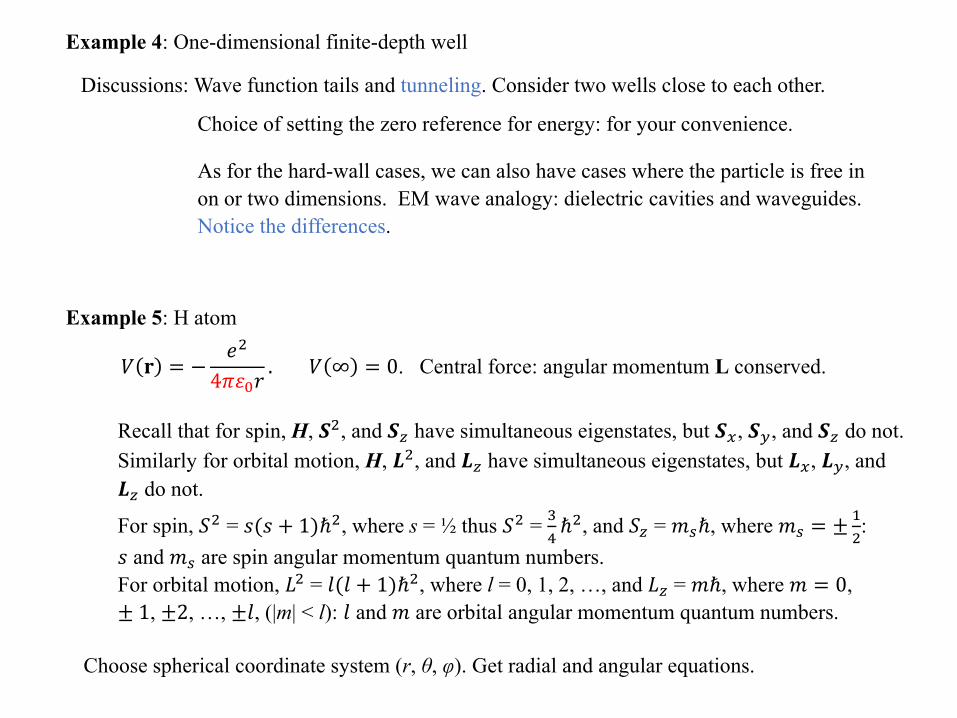
Example 4: One-dimensional finite-depth well
Discussions: Wave function tails and tunneling. Consider two wells close to each other.
Example 5: H atom
Choice of setting the zero reference for energy: for your convenience.
As for the hard-wall cases, we can also have cases where the particle is free in on or two dimensions. EM wave analogy: dielectric cavities and waveguides. Notice the differences.
𝑉𝑉 ∞ = 0. Central force: angular momentum L conserved.
Choose spherical coordinate system (r, θ, φ). Get radial and angular equations.
Recall that for spin, H, 𝑺𝑺2, and 𝑺𝑺𝑧𝑧 have simultaneous eigenstates, but 𝑺𝑺𝑥𝑥, 𝑺𝑺𝑦𝑦, and 𝑺𝑺𝑧𝑧 do not. Similarly for orbital motion, H, 𝑳𝑳2, and 𝑳𝑳𝑧𝑧 have simultaneous eigenstates, but 𝑳𝑳𝑥𝑥, 𝑳𝑳𝑦𝑦, and 𝑳𝑳𝑧𝑧 do not.
For spin, 𝑆𝑆2 = 𝑠𝑠(𝑠𝑠 + 1)ℏ2, where s = ½ thus 𝑆𝑆2 = 34ℏ2, and 𝑆𝑆𝑧𝑧 = 𝑚𝑚𝑠𝑠ℏ, where 𝑚𝑚𝑠𝑠 = ± 1
2:
𝑠𝑠 and 𝑚𝑚𝑠𝑠 are spin angular momentum quantum numbers. For orbital motion, 𝐿𝐿2 = 𝑙𝑙(𝑙𝑙 + 1)ℏ2, where l = 0, 1, 2, …, and 𝐿𝐿𝑧𝑧 = 𝑚𝑚ℏ, where 𝑚𝑚 = 0, ± 1, ±2, …, ±𝑙𝑙, (|m| < l): 𝑙𝑙 and 𝑚𝑚 are orbital angular momentum quantum numbers.
𝑉𝑉 𝐫𝐫 = −𝑒𝑒2
4𝜋𝜋𝜀𝜀0𝑟𝑟.

Choose spherical coordinate system (r, θ, φ). Get radial and angular equations by variable separation.
The solutions are 𝜓𝜓𝑛𝑛𝑛𝑛𝑚𝑚 𝑟𝑟,𝜃𝜃,𝜑𝜑 = 𝑅𝑅𝑛𝑛𝑛𝑛 𝑟𝑟 𝑌𝑌𝑛𝑛𝑚𝑚(𝜃𝜃,𝜑𝜑), where the spherical harmonics 𝑌𝑌𝑛𝑛𝑚𝑚 are solutions to angular momentum eigenvalue equations
𝑳𝑳2𝑌𝑌𝑛𝑛𝑚𝑚 𝜃𝜃,𝜑𝜑 = 𝑙𝑙(𝑙𝑙 + 1)ℏ2𝑌𝑌𝑛𝑛𝑚𝑚 𝜃𝜃,𝜑𝜑 , 𝑳𝑳𝑧𝑧𝑌𝑌𝑛𝑛𝑚𝑚 𝜃𝜃,𝜑𝜑 = 𝑚𝑚ℏ𝑌𝑌𝑛𝑛𝑚𝑚 𝜃𝜃,𝜑𝜑
Further separate θ and φ: 𝑌𝑌𝑛𝑛𝑚𝑚 𝜃𝜃,𝜑𝜑 = 𝛩𝛩𝑛𝑛𝑚𝑚 (𝜃𝜃) 12𝜋𝜋𝑒𝑒𝑖𝑖𝑚𝑚𝜑𝜑
Normalization with regard to ϕReal valued
l = 0, m = 0: s orbital. 𝑌𝑌00 𝜃𝜃,𝜑𝜑 =14𝜋𝜋
Angular momentum eigenvalues 𝐿𝐿2 = 0, 𝐿𝐿𝑧𝑧 = 0.
l = 1, m = 0, ±1: p orbitals
𝑌𝑌10 𝜃𝜃,𝜑𝜑 =34𝜋𝜋
cos𝜃𝜃
l = 1, m = 0: 𝑝𝑝𝑧𝑧 orbital: angular momentum eigenvalues 𝐿𝐿2 = 2ℏ2, 𝐿𝐿𝑧𝑧 = 0.
l = 1, m = ±1: linear combinations form 𝑝𝑝𝑥𝑥 and 𝑝𝑝𝑦𝑦 orbitals: angular momentum eigenvalues 𝐿𝐿2 = 2ℏ2, 𝐿𝐿𝑧𝑧 = ±ℏ.

l = 0, m = 0: s orbital 𝑌𝑌00 𝜃𝜃,𝜑𝜑 = 14𝜋𝜋
Angular momentum eigenvalues 𝐿𝐿2 = 0, 𝐿𝐿𝑧𝑧 = 0.
l = 1, m = 0, ±1: p orbitals
𝑌𝑌10 𝜃𝜃,𝜑𝜑 =34𝜋𝜋
cos𝜃𝜃 = 𝑝𝑝𝑧𝑧
l = 1, m = 0: 𝑝𝑝𝑧𝑧 orbital,angular momentum eigenvalues 𝐿𝐿2 = 2ℏ2, 𝐿𝐿𝑧𝑧 = 0.
l = 1, m = ±1: linear combinations form real-valued 𝑝𝑝𝑥𝑥 and 𝑝𝑝𝑦𝑦 orbitals, angular momentum eigenvalues 𝐿𝐿2 = 2ℏ2, 𝐿𝐿𝑧𝑧 = ±ℏ.
http://mathworld.wolfram.com/SphericalHarmonic.html
𝑌𝑌1,±1 𝜃𝜃,𝜑𝜑 = ∓ 38𝜋𝜋
sin𝜃𝜃 𝑒𝑒±𝑖𝑖𝜑𝜑
|𝑌𝑌10 𝜃𝜃,𝜑𝜑 |2
https://en.wikipedia.org/wiki/Spherical_harmonics
|𝑌𝑌1,±1 𝜃𝜃,𝜑𝜑 |2
𝑖𝑖2𝑌𝑌1,−1 + 𝑌𝑌1,−1 = 3
4𝜋𝜋sin𝜃𝜃 sin𝜑𝜑
12𝑌𝑌1,−1 − 𝑌𝑌1,−1 = 3
4𝜋𝜋sin𝜃𝜃 cos𝜑𝜑
⇒
You define polar angle from y axis, 𝜃𝜃𝑦𝑦, and polar angle from x axis, 𝜃𝜃𝑥𝑥.
cos𝜃𝜃𝑦𝑦 = sin𝜃𝜃 sin𝜑𝜑
cos𝜃𝜃𝑥𝑥 = sin𝜃𝜃 cos𝜑𝜑Easy to show
𝜃𝜃𝑦𝑦𝜃𝜃𝑥𝑥
s
p
d
f
𝑝𝑝𝑧𝑧𝑝𝑝𝑥𝑥𝑝𝑝𝑦𝑦

l = 1, m = 0, ±1: p orbitals
𝑌𝑌10 𝜃𝜃,𝜑𝜑 = 34𝜋𝜋
cos𝜃𝜃 ≡ 𝑝𝑝𝑧𝑧
l = 1, m = 0: 𝑝𝑝𝑧𝑧 orbital,angular momentum eigenvalues 𝐿𝐿2 = 2ℏ2, 𝐿𝐿𝑧𝑧 = 0.
l = 1, m = ±1: linear combinations form real-valued𝑝𝑝𝑥𝑥 and 𝑝𝑝𝑦𝑦 orbitals, angular momentum eigenvalues 𝐿𝐿2 = 2ℏ2, 𝐿𝐿𝑧𝑧 = ±ℏ.
𝑖𝑖2𝑌𝑌1,−1 + 𝑌𝑌1,1 = 3
4𝜋𝜋sin𝜃𝜃 sin𝜑𝜑 = 3
4𝜋𝜋cos𝜃𝜃𝑦𝑦 ≡ 𝑝𝑝𝑦𝑦
12𝑌𝑌1,−1 − 𝑌𝑌1,1 = 3
4𝜋𝜋sin𝜃𝜃 cos𝜑𝜑 = 3
4𝜋𝜋cos𝜃𝜃𝑥𝑥 ≡ 𝑝𝑝𝑥𝑥
Define polar angle from y axis, 𝜃𝜃𝑦𝑦, and polar angle from x axis, 𝜃𝜃𝑥𝑥.
cos𝜃𝜃𝑦𝑦 = sin𝜃𝜃 sin𝜑𝜑cos𝜃𝜃𝑥𝑥 = sin𝜃𝜃 cos𝜑𝜑
𝜃𝜃𝑦𝑦𝜃𝜃𝑥𝑥
Define polar angle from y axis, 𝜃𝜃𝑦𝑦, and polar angle from x axis, 𝜃𝜃𝑥𝑥.
Interesting to note that𝑝𝑝𝑧𝑧 is the eigenstate with 𝐿𝐿2 = 2ℏ2, 𝐿𝐿𝑧𝑧 = 0
(l = 1, m ≡ 𝑚𝑚𝑧𝑧 = 0);𝑝𝑝𝑦𝑦 is the eigenstate with 𝐿𝐿2 = 2ℏ2, 𝐿𝐿𝑦𝑦 = 0
(l = 1, 𝑚𝑚𝑦𝑦 = 0);𝑝𝑝𝑥𝑥 is the eigenstate with 𝐿𝐿2 = 2ℏ2, 𝐿𝐿𝑥𝑥 = 0
(l = 1, 𝑚𝑚𝑥𝑥 = 0).
https://en.wikipedia.org/wiki/Spherical_harmonics
s
p
d
f
𝑝𝑝𝑧𝑧𝑝𝑝𝑥𝑥𝑝𝑝𝑦𝑦

𝑝𝑝𝑧𝑧 = 𝑌𝑌10 𝜃𝜃,𝜑𝜑 =34𝜋𝜋
cos𝜃𝜃
𝑝𝑝𝑦𝑦 =𝑖𝑖2𝑌𝑌1,−1 + 𝑌𝑌1,1 =
34𝜋𝜋
sin𝜃𝜃 sin𝜑𝜑 =34𝜋𝜋
cos𝜃𝜃𝑦𝑦
𝑝𝑝𝑥𝑥 =12𝑌𝑌1,−1 − 𝑌𝑌1,1 =
34𝜋𝜋
sin𝜃𝜃 cos𝜑𝜑 =34𝜋𝜋
cos𝜃𝜃𝑥𝑥
Define polar angle from y axis, 𝜃𝜃𝑦𝑦, and polar angle from x axis, 𝜃𝜃𝑥𝑥.
cos𝜃𝜃𝑦𝑦 = sin𝜃𝜃 sin𝜑𝜑cos𝜃𝜃𝑥𝑥 = sin𝜃𝜃 cos𝜑𝜑
𝜃𝜃𝑦𝑦𝜃𝜃𝑥𝑥
FYI: 𝑝𝑝𝑥𝑥, 𝑝𝑝𝑦𝑦, 𝑝𝑝𝑧𝑧 orbitals and spherical harmonics
𝑝𝑝𝑧𝑧 is the eigenstate with 𝐿𝐿2 = 2ℏ2, 𝐿𝐿𝑧𝑧 = 0 (l = 1, m ≡ 𝑚𝑚𝑧𝑧 = 0);𝑝𝑝𝑦𝑦 is the eigenstate with 𝐿𝐿2 = 2ℏ2, 𝐿𝐿𝑦𝑦 = 0 (l = 1, 𝑚𝑚𝑦𝑦 = 0);𝑝𝑝𝑥𝑥 is the eigenstate with 𝐿𝐿2 = 2ℏ2, 𝐿𝐿𝑥𝑥 = 0 (l = 1, 𝑚𝑚𝑥𝑥 = 0).
https://en.wikipedia.org/wiki/Spherical_harmonics
𝑝𝑝𝑧𝑧 𝑝𝑝𝑥𝑥𝑝𝑝𝑦𝑦
The 𝑝𝑝𝑥𝑥, 𝑝𝑝𝑦𝑦, 𝑝𝑝𝑧𝑧 orbitals are real-valued. (Overall phase of one state irrelevant; the three are in phase.)
⇒𝑌𝑌1,1 =
𝑝𝑝𝑥𝑥 + 𝑖𝑖𝑝𝑝𝑦𝑦2
𝑌𝑌1,−1 =𝑝𝑝𝑥𝑥 − 𝑖𝑖𝑝𝑝𝑦𝑦
2

l = 2, m = 0, ±1, ±2: Five d orbitalsAngular momentum eigenvalues 𝐿𝐿2 = 6ℏ2.For m ≠ 0, linear combinations of 𝑌𝑌2,𝑚𝑚 form real-valued d orbitals.
l = 3, m = 0, ±1, ±2 , ±3: seven f orbitalsAngular momentum eigenvalues 𝐿𝐿2 = 12ℏ2.
https://en.wikipedia.org/wiki/Spherical_harmonics
s
p
d
f
𝑝𝑝𝑧𝑧
𝑝𝑝𝑥𝑥𝑝𝑝𝑦𝑦
x
z
y⊙
These are solutions to the angular equation, which is the angular momentum eigenvalue equation.

The overall solutions are 𝜓𝜓𝑛𝑛𝑛𝑛𝑚𝑚 𝑟𝑟,𝜃𝜃,𝜑𝜑 = 𝑅𝑅𝑛𝑛𝑛𝑛 𝑟𝑟 𝑌𝑌𝑛𝑛𝑚𝑚(𝜃𝜃,𝜑𝜑).
For all central forces, the angular solutions 𝑌𝑌𝑛𝑛𝑚𝑚(𝜃𝜃,𝜑𝜑) are the same.
For a general central force, the radial solutions 𝑅𝑅𝑛𝑛𝑛𝑛 𝑟𝑟 correspond to energy eigenvalues 𝐸𝐸𝑛𝑛𝑛𝑛.
For the Coulomb force of a point charge, energy eigenvalues 𝐸𝐸𝑛𝑛𝑛𝑛 is degenerate for all l, thus simply 𝐸𝐸𝑛𝑛.
n = 1, 2, 3, … l = 0, 1, 2, …, n−1 𝐸𝐸𝑛𝑛 = −1
(4𝜋𝜋𝜀𝜀0)2𝑚𝑚𝑒𝑒4
2ℏ21𝑛𝑛2
http://staff.mbi-berlin.de/hertel/physik3/chapter8/8.3html/01__99.png
|𝑟𝑟𝑅𝑅𝑛𝑛𝑛𝑛 𝑟𝑟 |2
https://d2jmvrsizmvf4x.cloudfront.net/oVigeAgPQwC2STwkBOQr_01__100.png
𝑅𝑅10 𝑟𝑟
𝑅𝑅20 𝑟𝑟
𝑅𝑅30 𝑟𝑟
𝑅𝑅21 𝑟𝑟
𝑅𝑅31 𝑟𝑟 𝑅𝑅32 𝑟𝑟

Visualization of 𝑅𝑅𝑛𝑛𝑛𝑛 𝑟𝑟
n = 1, 2, 3, … l = 0, 1, 2, …, n−1
http://staff.mbi-berlin.de/hertel/physik3/chapter8/8.3html/01__99.png
|𝑟𝑟𝑅𝑅21 𝑟𝑟 |2
https://d2jmvrsizmvf4x.cloudfront.net/oVigeAgPQwC2STwkBOQr_01__100.png
𝑅𝑅𝑛𝑛𝑛𝑛 𝑟𝑟
𝑅𝑅10 𝑟𝑟
𝑅𝑅20 𝑟𝑟
𝑅𝑅30 𝑟𝑟
𝑅𝑅21 𝑟𝑟
𝑅𝑅31 𝑟𝑟𝑅𝑅32 𝑟𝑟
|𝑟𝑟𝑅𝑅10 𝑟𝑟 |2
|𝑟𝑟𝑅𝑅20 𝑟𝑟 |2
|𝑟𝑟𝑅𝑅30 𝑟𝑟 |2|𝑟𝑟𝑅𝑅𝑛𝑛𝑛𝑛 𝑟𝑟 |2
|𝑟𝑟𝑅𝑅31 𝑟𝑟 |2
|𝑟𝑟𝑅𝑅32 𝑟𝑟 |2
𝐸𝐸1 = −13.6 eV
Bohr radius 𝑎𝑎0 = 4𝜋𝜋𝜀𝜀0ℏ2
𝑚𝑚𝑒𝑒2
𝐸𝐸𝑛𝑛 = −1
4𝜋𝜋𝜀𝜀0 2𝑚𝑚𝑒𝑒4
2ℏ21𝑛𝑛2
= −1
4𝜋𝜋𝜀𝜀0𝑒𝑒2
2𝑎𝑎01𝑛𝑛2
𝑎𝑎0 = 0.53 Å
𝑎𝑎0 = 0.53 Å

https://en.wikipedia.org/wiki/Atomic_orbital
Visualization of the overall wave functions 𝜓𝜓𝑛𝑛𝑛𝑛𝑚𝑚 𝑟𝑟,𝜃𝜃,𝜑𝜑 = 𝑅𝑅𝑛𝑛𝑛𝑛 𝑟𝑟 𝑌𝑌𝑛𝑛𝑚𝑚(𝜃𝜃,𝜑𝜑)

𝑎𝑎0 = 0.53 Å
𝐸𝐸1 = 12𝑉𝑉 𝑎𝑎 = −13.6 eV
𝑉𝑉 𝑎𝑎 = 2𝐸𝐸1 = −27.2 eV
http://www.starkeffects.com/hydrogen_atom_wavefunctions.shtml

Potential well shapes and energy level distributions
https://www.cambridge.org/core/books/applied-nanophotonics/electrons-in-potential-wells-and-in-solids/D1A1D672320B55539DE286196D51EF47
https://en.wikibooks.org/wiki/Materials_in_Electronics/Confined_Particles/1D_Finite_Wells
http://www.starkeffects.com/hydrogen_atom_wavefunctions.shtml

Highlights and Remarks
Quantum mechanics is not weird.We are familiar with waves, superposition, and coherence.
A possible reason it may look hard/weird: For other waves, both the amplitude and the intensity are observable quantities. In quantum mechanics, the amplitude per se is not observable while the analog of intensity is probability.
Analogy helps. Stationary states are like modes of electromagnetic wave. But, we also notice differences.
Physical quantities are real. ⇒ Amplitudes of other waves are real. We use complex numbers as a math tool. For example, a single tone is the sum of a positive- and a negative-frequency Fourier component. Amplitudes in quantum mechanics are complex.
Schrödinger equation vs. other wave equations.
i vs. j as −1.
𝛻𝛻2ψ 𝐫𝐫 = −2𝑚𝑚ℏ2
[ℏ𝜔𝜔 − 𝑉𝑉 𝐫𝐫 ]ψ 𝐫𝐫 𝛻𝛻2ψ 𝐫𝐫 = −𝜔𝜔2
𝑐𝑐2𝑛𝑛2ψ 𝐫𝐫vs. for stationary states.
𝑒𝑒−𝑖𝑖𝜔𝜔𝑡𝑡 𝑒𝑒𝑗𝑗𝜔𝜔𝑡𝑡vs.
𝑒𝑒𝑖𝑖(𝑘𝑘𝑥𝑥−𝜔𝜔𝑡𝑡) 𝑒𝑒𝑗𝑗(𝜔𝜔𝑡𝑡−𝑘𝑘𝑥𝑥)vs.
Refractive index
A quantity e.g. Ez, V or Iin 1D transmission line
There are no 1D dielectric cavities!

We are familiar with the vector space, linear algebra.Again, complex amplitudes per se are not observable in quantum mechanics.
Amplitudes in quantum mechanics are complex. Inner products involve taking complex conjugates.
(The bra is the conjugate transpose of the ket)Complex amplitudes are used elsewhere for mathematical convenience.
Revisit H+
Limited scope of this QM primer: one-particle

The electron is shared by the two protons, resulting in two stationary states:
Bonding: |0⟩ = 12
(|L⟩ + |R⟩), lower-energy, symmetric
Antibonding: |1⟩ = 12
(|L⟩ − |R⟩), higher-energy, antisymmetric
Revisit H2+
|L⟩: the electron associated with the left H atom
|R⟩: the electron associated with the right H atom
⟨𝐫𝐫|𝐿𝐿⟩ = ψ𝐿𝐿 𝜕𝜕
ψ𝐿𝐿 𝐫𝐫
ψ𝑅𝑅 𝐫𝐫
⟨𝐫𝐫|𝑅𝑅⟩ = ψ𝑅𝑅 𝜕𝜕
Convenient to take the two atomic orbitals (1s) centered at the two nuclei as the two basis vectors |L⟩ and |R⟩.
Question:Do you see a problem with this choice of the basis set?

The electron is shared by the two protons, resulting in two stationary states:
Bonding: |0⟩ = 12
(|L⟩ + |R⟩), lower-energy, symmetric
Antibonding: |1⟩ = 12
(|L⟩ − |R⟩), higher-energy, antisymmetric
Revisit H2+
|L⟩: the electron associated with the left H atom
|R⟩: the electron associated with the right H atom
⟨𝐫𝐫|𝐿𝐿⟩ = ψ𝐿𝐿 𝜕𝜕
ψ𝐿𝐿 𝐫𝐫
ψ𝑅𝑅 𝐫𝐫
⟨𝐫𝐫|𝑅𝑅⟩ = ψ𝑅𝑅 𝜕𝜕
Convenient to take the two atomic orbitals (1s) centered at the two nuclei as the two basis vectors |L⟩ and |R⟩.
But, there is a problem: ⟨𝐿𝐿|𝑅𝑅⟩ = �𝑑𝑑3𝐫𝐫ψ𝐿𝐿∗ 𝜕𝜕 ψ𝑅𝑅 𝜕𝜕 ≠ 0
Limited scope of this QM primer: one-particle
For example, another issue (approximation) w/ the above H2+ picture:
We kept the two protons fixed.

Homework 1
Due date Thu 1/30 okay?


