SPIN MATRICES FOR ARBITRARY SPIN - Reed College › physics › faculty › wheeler... · 4 Spin...

Remarks concerning the explicit construction of

SPIN MATRICES FOR ARBITRARY SPIN

Nicholas Wheeler, Reed College Physics Department

August 2000

Introduction. This subject lies a bit skew to my main areas of interest. I feel aneed, therefore, to explain why, somewhat to my surprise, I find myself writingabout it today—lacing my boots, as it were, in preparation for the hike thatwill take me to places in which I do have an established interest.

On 3 November 1999, Thomas Wieting presented at Reed College a physicsseminar entitled “The Penrose Dodecahedron.” That talk was inspired by therecent publication of a paper by Jordan E. Massad & P. K. Arvind,1 which inturn derived from an idea sketched in Roger Penrose’s Shadows of the Mind() and developed in greater detail in a paper written collaboratively byPenrose and J. Zamba.2 Massad & Aravind speculate that Penrose drew hisinspiration from Asher Peres, but there is no need to speculate in this regard; alittle essay entitled “The Artist, the Physicist and the Waterfall” which appearson page 30 of the February issue of Scientific American describes theentangled source of Penrose’s involvement in fascinating detail.3 Not at allspeculative is their observation that Penrose/Zamba drew critically upon anidea incidental to work reported by the then -year-old Etorre Majorana in aclassic paper having to do with the spin-reversal of polarized particles/atomsin time-dependent magnetic fields.4 Massad/Aravind remark that “whateverthe genesis of [Penrose/Zamba’s line of argument, they] deftly manipulateda geometrical picture of quantum spins due to Majorana to deduce all theproperties of [certain] rays they needed in their proofs of the Bell and Bell-Kochen-Specker theorems.”

1 “The Penrose dodecahedron revisited,” AJP 67, 631 (1999).2 “On Bell non-locality without probabilities: More curious geometry,” Stud.

Hist. Phil. Sci. 24, 697 (1993). The paper is based upon Zamba’s thesis.3 The story involves Maurits C. Escher in an unexpected way, but hinges on

the circumstance that Penrose was present at a seminar given by Peres in ,the upshot of which was published as “Two simple proofs of the Kochen-Speckertheorem,” J. Phys. A: Math. Gen. 24, L175 (1991). See also Peres’ QuantumTheory: Concepts & Methods ().

4 “Atomi orientati in campo magnetico variabile,” Nuovo Cimento 9, 43–50(1932).

2 Spin matrices

Massad & Avarind suggest that “an even bigger virtue of the Majoranaapproach [bigger, that is to say, than its computational efficiency] is that itseems to have hinted at the existence of the Penrose dodecahedron in the firstplace,” but observe that “the Majorana picture of spin, while very elegantand also remarkably economical for the problem at hand, is still unfamiliar tothe vast majority of physicists,” so have undertaken to construct a “poor man’sversion” of the Penrose/Zamba paper which proceeds entirely without referenceto Majorana’s techniques.

In their §2, Massad & Aravind draw upon certain results which theyconsider “standard” to the quantum theory of angular momentum, citing suchworks as the text by J. J. Sakuri5 and the monograph by A. R. Edmonds.6

But I myself have never had specific need of that “standard” material, andhave always found it—at least as it is presented in the sources most familiar tome7—to be so offputtingly ugly that I have been happy to avoid it; what mayindeed be “too familiar for comment” to many/most of the world’s quantumphysicists remains, I admit, only distantly familiar to me. So I confronted afreshthis elementary question:

What are the angular momentum matricescharacteristic of a particle of (say) spin 3

2?

My business here is to describe a non-standard approach to the solution of suchquestions, and to make some comments.

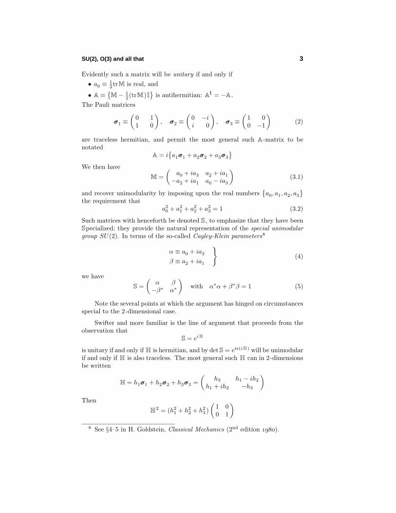
SU(2), O(3) and all that. I begin with brief review of some standard material,partly to underscore how elementary are the essential ideas, and partly toestablish some notational conventions. It is upon this elementary foundationthat we will build.

Let M be any 2× 2 matrix. From det(M− λI) = λ2− (trM)λ+ det M weby the Cayley-Hamilton theorem have

M –1 =(trM)I−M

det Munless M is singular

which gives

M –1 = (trM)I−M if M is “unimodular” : det M = 1

Trivially, any 2× 2 matrix M can be written

M = 12 (trM)I +

{M− 1

2 (trM)I}︸︷︷︸ (1.1)

traceless

while we have just established that in unimodular cases

M –1 = 12 (trM)I−

{M− 1

2 (trM)I}

(1.2)

5 Modern Quantum Mechanics ().6 Angular Momentum in Quantum Mechanics ().7 Leonard Schiff, Quantum Mechanics (3rd edition ), pages 202–203;

J. L. Powell & B. Crasemann, Quantum Mechanics (), §10–4.

SU(2), O(3) and all that 3

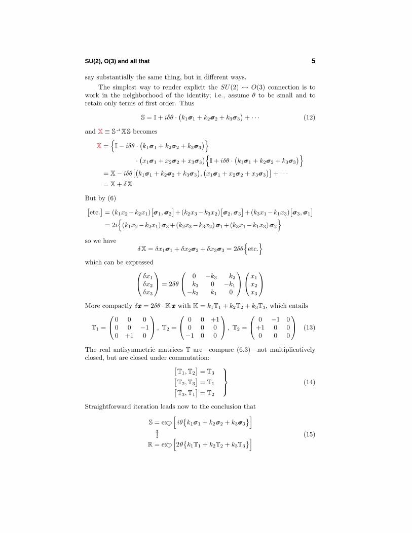
Evidently such a matrix will be unitary if and only if• a0 ≡ 1

2 trM is real, and

• A ≡{M− 1

2 (trM)I}

is antihermitian: At = −A .The Pauli matrices

σσ1 ≡(

0 11 0

), σσ2 ≡

(0 −ii 0

), σσ3 ≡

(1 00 −1

)(2)

are traceless hermitian, and permit the most general such A -matrix to benotated

A = i{a1σσ1 + a2σσ2 + a3σσ3

}We then have

M =(

a0 + ia3 a2 + ia1

−a2 + ia1 a0 − ia3

)(3.1)

and recover unimodularity by imposing upon the real numbers{a0, a1, a2, a3

}the requirement that

a20 + a2

1 + a22 + a2

3 = 1 (3.2)

Such matrices with henceforth be denoted S , to emphasize that they have beenSpecialized; they provide the natural representation of the special unimodulargroup SU(2). In terms of the so-called Cayley-Klein parameters8

α ≡ a0 + ia3

β ≡ a2 + ia1

}(4)

we have

S =(

α β−β∗ α∗

)with α∗α + β∗β = 1 (5)

Note the several points at which the argument has hinged on circumstancesspecial to the 2-dimensional case.

Swifter and more familiar is the line of argument that proceeds from theobservation that

S = eiH

is unitary if and only if H is hermitian, and by det S = etr(iH ) will be unimodularif and only if H is also traceless. The most general such H can in 2-dimensionsbe written

H = h1σσ1 + h2σσ2 + h3σσ3 =(

h3 h1 − ih2

h1 + ih2 −h3

)

Then

H2 = (h21 + h2

2 + h23 )

(1 00 1

)8 See §4–5 in H. Goldstein, Classical Mechanics (2nd edition ).

4 Spin matrices

which implies and is implied by the statements

σσ21 = σσ2

2 = σσ23 = I (6.1)

σσ1σσ2 = −σσ2σσ1



(6.2)

Also demonstrably true—but not implicit in the preceding line of argument—are the statements

σσ1σσ2 = i σσ3



(6.3)

Results now in hand lead us to write

hhh = θkkk : kkk a real unit 3-vector

and obtain

S = exp[iθ

{k1σσ1 + k2σσ2 + k3σσ3

}]= cos θ · I + i sin θ ·


}(7.1)

=(

cos θ + ik3 sin θ (k2 + ik1) sin θ−(k2 − ik1) sin θ cos θ − ik3 sin θ

)(7.2)

in which notation the Cayley-Klein parameters (4) become

α = cos θ + ik3 sin θ

β = (k2 + ik1) sin θ

}(8)

The Cayley-Klein parameters were introduced by Felix Klein in connectionwith the theory of tops; i.e., as aids to the description of the 3-dimensionalrotation group O(3), with which we have now to establish contact. This we willaccomplish in two different ways. The more standard approach is to introducethe traceless hermitian matrix

X ≡ x1σσ1 + x2σσ2 + x3σσ3 =(

x3 x1 − ix2

x1 + ix2 −x3

)(9)

and to notice that X �−→ X ≡ S –1 XS sends X into a matrix which is againtraceless hermitian, and which has the same determinant:

det X = det X = −(x21 + x2

2 + x23 )

Evidently

X �−→ S –1 XS ≡(

x3 x1 − ix2

x1 + ix2 −x3

): S ∈ SU(2) (10)

and x1

x2

x3

�−→ R

x1

x2

x3

≡

x1

x2

x3

: R ∈ O(3) (11)

SU(2), O(3) and all that 5

say substantially the same thing, but in different ways.The simplest way to render explicit the SU(2) ↔ O(3) connection is to

work in the neighborhood of the identity; i.e., assume θ to be small and toretain only terms of first order. Thus

S = I + iδθ ·(k1σσ1 + k2σσ2 + k3σσ3

)+ · · · (12)

and X ≡ S –1 XS becomes

X ={

I− iδθ ·(k1σσ1 + k2σσ2 + k3σσ3

)}·(x1σσ1 + x2σσ2 + x3σσ3

){I + iδθ ·

(k1σσ1 + k2σσ2 + k3σσ3

)}= X− iδθ

[(k1σσ1 + k2σσ2 + k3σσ3

),(x1σσ1 + x2σσ2 + x3σσ3

)]+ · · ·

= X + δX

But by (6)[etc.

]= (k1x2−k2x1)

[σσ1, σσ2

]+(k2x3−k3x2)

[σσ2, σσ3

]+(k3x1−k1x3)

[σσ3, σσ1

]= 2i

{(k1x2−k2x1)σσ3 +(k2x3−k3x2)σσ1 +(k3x1−k1x3)σσ2

}so we have

δX = δx1σσ1 + δx2σσ2 + δx3σσ3 = 2δθ{

etc.}

which can be expressed δx1

δx2

δx3

= 2δθ

0 −k3 k2

k3 0 −k1

−k2 k1 0

x1

x2

x3

More compactly δxxx = 2δθ ·Kxxx with K = k1T1 + k2T2 + k3T3, which entails

T1 =

0 0 0

0 0 −10 +1 0

, T2 =

0 0 +1

0 0 0−1 0 0

, T2 =

0 −1 0

+1 0 00 0 0

(13)

The real antisymmetric matrices T are—compare (6.3)—not multiplicativelyclosed, but are closed under commutation:[

T1,T2

]= T3[

T2,T3

]= T1[

T3,T1

]= T2

(14)

Straightforward iteration leads now to the conclusion that

S = exp[iθ


}]↑� (15)

R = exp[2θ

{k1T1 + k2T2 + k3T3

}]

6 Spin matrices

If{x1, x2, x3

}refer to a right hand frame, then R describes a right handed

rotation through angle 2θ about the unit vector kkk. Notice that—and howelementary is the analytical origin of the fact that—the association (15) isbiunique: reading from (7.1) we see that

S→ −S as θ advances from 0 to π

and that S returns to its initial value at θ = 2π. But from the quadraticstructure of X ≡ S –1 XS we see that ±S both yield the same X ; i.e., that R

returns to its initial value as θ advances from 0 to π, and goes twice around asS goes once around. One speaks in this connection of the “double-valuedness ofthe spin representations of the rotation group,” and it is partly to place us inposition to do so—but mainly to prepare for things to come—that I turn nowto an alternative approach to the issue just discussed.

Introduce the

2-component spinor ξ ≡(

uv

)(16)

(which is by nature just a complex 2-vector) and consider transformations ofthe form

ξ �−→ ξ ≡ S ξ (17)

From the unitarity of S (unimodularity is in this respect not needed) it followsthat

ξtξ = ξtξ (18)

In more explicit notation we have(uv

)=

(α β−β∗ α∗

) (uv

)(19)

andu∗u + v∗v = u∗u + v∗v (20)

At (8) we acquired descriptions of α and β to which we can now assign rotationalinterpretations in Euclidean 3-space. But how to extract O(3) from (19)without simply hiking backward along the path we have just traveled?

Kramer’s method for recovering O(3). Hendrik Anthony Kramers (–)was very closely associated with many/most of the persons and events thatcontributed to the invention of quantum mechanics, but his memory lives in theshadow of such giants as Bohr, Pauli, Ehrenfest, Born, Dirac. Max Dresden, in afascinating recent biography,9 has considered why Kramers career fell somewhatshort of his potential, and has concluded that a contributing factor was hisexcessive interest in mathematical elegance and trickery. It is upon one (widelyuncelebrated) manifestation of that personality trait that I base much of whatfollows.

9 H. A. Kramers: Between Tradition and Revolution ().

Introduction to Kramer’s method 7

In / Kramers developed an algebraic approach to the quantumtheory of spin/angular momentum which—though clever, and computationallypowerful—gained few adherents.10 A posthumous account of Kramers’ methodwas presented in a thin monograph by one of his students,11 and I myself havewritten about the subject on several occasions.12

We proceed from this question:

What is the

uu

uvvv

→

uu

uvvv

induced by (19)?

Immediately uu

uvvv

=

(αu + βv)(αu + βv)

(αu + βv)(−β∗u + α∗v)(−β∗u + α∗v)(−β∗u + α∗v)

Entrusting the computational labor to Mathematica, we find

=

α2 2αβ β2

−αβ∗ αα∗ − ββ∗ βα∗

(β∗)2 −2α∗β∗ (α∗)2

uu

uvvv

(21.1)

which we agree to abbreviate

ζζζ = Qζζζ (21.2)

where Q is intended to suggest “quadratic.”

At an early point in his argument Kramers develops an interest in null3-vectors. Such a vector, if we are to avoid triviality, must necessarily becomplex. He writes

aaa = bbb + iccc : require b2 = c2 and bbb···ccc = 0 (22)

Since a21 + a2

2 + a23 = 0 entails a3 = ±i

√(a1 + ia2)(a1 − ia2) it becomes fairly

natural to introduce complex variables

u ≡√a1 − ia2

v ≡ i√a1 + ia2

10 Among those few was E. P. Wigner. Another was John L. Powell who, aftergraduating from Reed College in , became a student of Wigner, learnedKramers’ method from him, and provided an account of the subject in §7–2 ofhis beautiful text.7 Powell cites the Appendix to Chapter VII in R. Courant &D. Hilbert, Methods of Mathematical Physics, Volume I , where W. Magnus hastaken some similar ideas from “unpublished notes by the late G. Herglotz.”

11 H. Brinkman, Applications of Spinor Invariants in Atomic Physics ().12 See, for example, “Algebraic theory of spherical harmonics” ().

8 Spin matrices

Thena1 = 1

2 (u2 − v2)

a2 = i 12 (u2 + v2)

a3 ≡ −iuv

(23)

The aaa(u, v) thus defined has the property that

aaa(u, v) = aaa(−u,−v) (24)

We conclude that, as (u, v) ranges over complex 2-space, aaa(u, v) ranges twiceover the set of null 3-vectors, of which (23) provides a parameterized description.

Thus prepared, we ask: What is the aaa �−→ aaa that results when S acts by(17) on the parameter space? We saw at (21) that (17) induces

ζζζ �−→ ζζζ = Qζζζ (25)

while at (23) we obtained

aaa = Cζζζ with C ≡ 12

1 0 −1

i 0 i0 −2 0

(26)

So we have

aaa �−→ aaa =Raaa (27.1)R ≡ CQC –1 (27.2)

Mathematica is quick to inform us that, while R is a bit of a mess, it is amess with the property that every element is manifestly conjugation-invariant(meaning real). And, moreover, that RT R = I . In short,

R is a real rotation matrix, an element of O(3)

To sharpen that statement we again (in the tradition of Sophus Lie) retreatto the neighborhood of the identity and work in first order; from (8) we have

α = 1 + ik3 δθ

β = (k2 + ik1)δθ

}(28)

Substitute into Q , abandon terms of second order and obtain

Q = I +

2ik3 2(k2 + ik1) 0−(k2 − ik1) 0 (k2 + ik1)

0 −2(k2 − ik1) −2ik3

δθ + · · ·

whence (by calculation which I have entrusted to Mathematica)

R = I−

0 −k3 +k1

+k3 0 −k2

−k1 +k2 0

2δθ + · · · (29)

↑Note!

Spin matrices by Kramer’s method 9

This describes a doubled-angle rotation about kkk which is, however, retrograde.13

The preceding argument has served—redundantly, but by different means—to establish

SU(2)←←→ O(3)

The main point of the discussion lies, however, elsewhere. We now back up to(21) and head off in a new direction.

Spin matrices by Kramer’s method. For reasons that will soon acquire a highdegree of naturalness, we agree at this point in place of (17) to write

ξ( 12 ) �−→ ξ( 1

2 ) ≡ S( 12 ) ξ( 1

2 ) (30)

and to adopt this abbreviation of (21):

ζ(1) �−→ ζ(1) ≡ Q(1) ζ(1)

Mathematica informs us that the 3× 3 matrix Q(1) is unimodular

det Q(1) = 1

but not unitary. . .nor do we expect it to be: the invariance of u∗u+v∗v impliesthat not of (uu)∗(uu) + (uv)∗(uv) + (vv)∗(vv) but of

(u∗u + v∗v)2 = (uu)∗(uu) + 2(uv)∗(uv) + (vv)∗(vv)

= ζt(1)G(1)ζ(1)

G(1) ≡

1 0 0

0 2 00 0 1

Define

ξ(1) ≡√

G ζ(1) with√

G =

1 0 0

0√

2 00 0 1

(31)

Then the left side of

ξt(1)ξ(1) = (u∗u + v∗v)2 =[ξt( 1

2 )ξ( 12 )

]2 (32)

is invariant under under the induced transformation

ξ(1) �−→ ξ(1) ≡ S(1) ξ(1) (33.1)

S(1) ≡ G+ 12 ·Q(1) ·G− 1

2 (33.2)

because the right side is invariant under ξ( 12 ) �−→ ξ( 1

2 ) ≡ S( 12 ) ξ( 1

2 ). We are

13 To achieve prograde rotation in the essay just cited I tacitly abandonedPauli’s conventions. I had reason at (2) to adopt those conventions, and herepay the price. It was to make things work out as nicely as they have that at(23) I departed slightly from the corresponding equations (27) in “Algebraictheory. . . ”12

10 Spin matrices

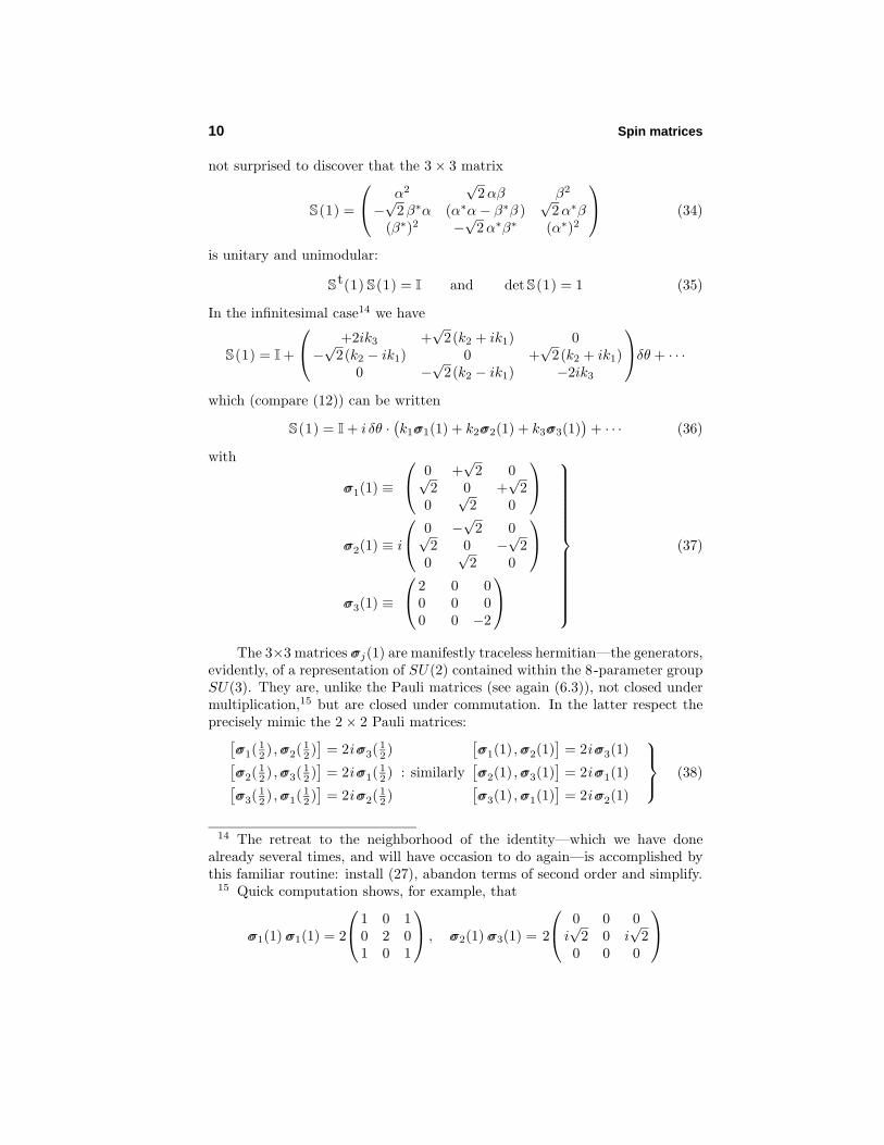
not surprised to discover that the 3× 3 matrix

S(1) =

α2

√2αβ β2

−√

2β∗α (α∗α− β∗β )√

2α∗β(β∗)2 −

√2α∗β∗ (α∗)2

(34)

is unitary and unimodular:

St(1) S(1) = I and det S(1) = 1 (35)

In the infinitesimal case14 we have

S(1) = I +

+2ik3 +

√2(k2 + ik1) 0

−√

2(k2 − ik1) 0 +√

2(k2 + ik1)0 −

√2(k2 − ik1) −2ik3

δθ + · · ·

which (compare (12)) can be written

S(1) = I + i δθ ·(k1σσ1(1) + k2σσ2(1) + k3σσ3(1)

)+ · · · (36)

with

σσ1(1) ≡

0 +

√2 0√

2 0 +√

20

√2 0

σσ2(1) ≡ i

0 −

√2 0√

2 0 −√

20

√2 0

σσ3(1) ≡

2 0 0

0 0 00 0 −2

(37)

The 3×3 matrices σσj(1) are manifestly traceless hermitian—the generators,evidently, of a representation of SU(2) contained within the 8-parameter groupSU(3). They are, unlike the Pauli matrices (see again (6.3)), not closed undermultiplication,15 but are closed under commutation. In the latter respect theprecisely mimic the 2× 2 Pauli matrices:[

σσ1(12 ) , σσ2(

12 )

]= 2iσσ3(

12 )[

σσ2(12 ) , σσ3(

12 )

]= 2iσσ1(

12 )[

σσ3(12 ) , σσ1(

12 )

]= 2iσσ2(

12 )

: similarly

[σσ1(1) , σσ2(1)

]= 2iσσ3(1)[

σσ2(1) , σσ3(1)]

= 2iσσ1(1)[σσ3(1) , σσ1(1)

]= 2iσσ2(1)

(38)

14 The retreat to the neighborhood of the identity—which we have donealready several times, and will have occasion to do again—is accomplished bythis familiar routine: install (27), abandon terms of second order and simplify.

15 Quick computation shows, for example, that

σσ1(1) σσ1(1) = 2

1 0 1

0 2 01 0 1

, σσ2(1) σσ3(1) = 2

0 0 0

i√

2 0 i√

20 0 0

Bare bones of the quantum theory of angular momentum 11

There are, however, some notable differences, which will acquire importance:

σσ21( 1

2 ) + σσ22( 1

2 ) + σσ23( 1

2 ) = 3(

1 00 1

)(39.05)

σσ21(1) + σσ2

2(1) + σσ23(1) = 8

1 0 0

0 1 00 0 1

(39.10)

We are within sight now of our objective, which is to say: we are inpossession of technique sufficient to construct (2# + 1)-dimensional tracelesshermitian triples {

σσ1(#), σσ2(#), σσ3(#)}

: # = 32 , 2,

52 , . . . (40)

with properties that represent natural extensions of those just encountered. Butbefore looking to the details, I digress to assemble the. . .

Bare bones of the quantum theory of angular momentum. Classical mechanicsengenders interest in the construction LLL = rrr × ppp ; i.e., in

L1 = x2p3 − x3p2

L2 = x3p1 − x1p3

L3 = x1p2 − x2p1

The primitive Poisson bracket relations

[xm, xn] = [pm, pn] = 0 and [xm, pn] = δmn

are readily found to entail[L1, L2] = L3

[L2, L3] = L1

[L3, L1] = L2

and[L1, L

2] = [L2, L2] = [L3, L

2] = 0

where L2 ≡ LLL···LLL = L21 +L2

2 +L23. In quantum theory those classical observables

become hermitian operators L1, L2, L3 and L2 ≡ L21 + L2

2 + L23 and Dirac’s

principle [xm, pn] = δmn −→ [xm, pn] = i I gives rise to commutation relationsthat mimic the preceding Poisson bracket relations:

[L1, L2] = i L3

[L2, L3] = i L1

[L3, L1] = i L2

(41)

[L1, L2] = [L2, L2] = [L3, L2] = 0 (42)

12 Spin matrices

The function-theoretic approach to the subject16 proceeds from

x → xxx · and p → �

i∇∇∇

and leads (one works actually in spherical coordinates) to the theory of sphericalharmonics

Y m� (xxx) :

{# = 0, 1, 2, . . .m = −#,−(#− 1), . . . ,−1, 0,+1, . . . ,+(#− 1),+#

L2Y m� = #(# + 1) · Y m

�

L3Ym� = m · Y m

�

}(43)

But the subject admits also of algebraic development, and that approach, whileit serves to reproduce the function-theoretic results just summarized, leads alsoto a physically important algebraic extension

# = 0, 12 , 1,

32 , 2,

52 . . . (44)

of the preceding theory.

One makes a notational adjustment

L → J

to emphasize that one is talking now about an expanded subject (fusion of the“theory of orbital angular momentum” and a “theory of intrinsic spin”) andintroduces non-hermitian “ladder operators”

J+ = J1 + iJ2

J− = J1 − iJ2

}(45)

One finds the #th eigenspace of J2 to be (2# + 1)-dimensional, and uses J3 toresolve the degeneracy. Let the normalized simultaneous eigenvectors of J2 andJ3 be denoted |#,m):

J2 |#,m) = #(# + 1) 2 · |#,m)J3 |#,m) = m · |#,m)

(#,m|# ′,m′) = δ��′δmm′

(46)

One finds thatJ+|#,m) ∼ |#,m + 1) : m < #

J+|#,m) = 0 : m = #

}(47.1)

J−|#,m) ∼ |#,m− 1) : m > −#J+|#,m) = 0 : m = −#

}(47.2)

16 See D. Griffiths’ Introduction to Quantum Mechanics (), §§4.1.2 and4.3 or, indeed, any quantum text. For an approach (Kramers’) more in keepingwith the spirit of the present discussion see again my “Algebraic approach. . . ”12

Bare bones of the quantum theory of angular momentum 13

and that one has to introduce ugly renormalization factors

1 √

#(# + 1)−m(m± 1)(48)

to turn the ∼’s into =’s.

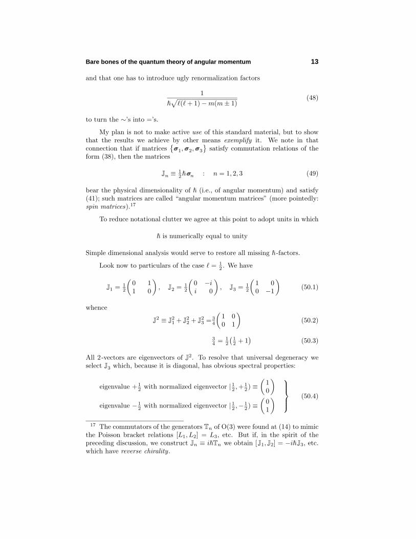
My plan is not to make active use of this standard material, but to showthat the results we achieve by other means exemplify it. We note in thatconnection that if matrices

{σσ1, σσ2, σσ3

}satisfy commutation relations of the

form (38), then the matrices

Jn ≡ 12 σσn : n = 1, 2, 3 (49)

bear the physical dimensionality of (i.e., of angular momentum) and satisfy(41); such matrices are called “angular momentum matrices” (more pointedly:spin matrices).17

To reduce notational clutter we agree at this point to adopt units in which

is numerically equal to unity

Simple dimensional analysis would serve to restore all missing -factors.

Look now to particulars of the case # = 12 . We have

J1 = 12

(0 11 0

), J2 = 1

2

(0 −ii 0

), J3 = 1

2

(1 00 −1

)(50.1)

whence

J2 ≡ J21 + J2

2 + J23 = 3

4

(1 00 1

)(50.2)

34 = 1

2

(12 + 1

)(50.3)

All 2-vectors are eigenvectors of J2. To resolve that universal degeneracy weselect J3 which, because it is diagonal, has obvious spectral properties:

eigenvalue + 12 with normalized eigenvector | 12 ,+ 1

2 ) ≡(

10

)

eigenvalue − 12 with normalized eigenvector | 12 ,− 1

2 ) ≡(

01

) (50.4)

17 The commutators of the generators Tn of O(3) were found at (14) to mimicthe Poisson bracket relations [L1, L2] = L3, etc. But if, in the spirit of thepreceding discussion, we construct Jn ≡ i Tn we obtain [J1, J2] = −i J3, etc.which have reverse chirality .

14 Spin matrices

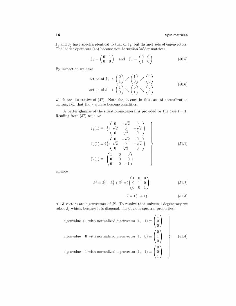
J1 and J2 have spectra identical to that of J3, but distinct sets of eigenvectors.The ladder operators (45) become non-hermitian ladder matrices

J+ =(

0 10 0

)and J− =

(0 01 0

)(50.5)

By inspection we have

action of J+ :(

01

)↗

(10

)↗

(00

)

action of J− :(

10

)↘

(01

)↘

(00

) (50.6)

which are illustrative of (47). Note the absence in this case of normalizationfactors; i.e., that the ∼’s have become equalities.

A better glimpse of the situation-in-general is provided by the case # = 1.Reading from (37) we have

J1(1) ≡ 12

0 +

√2 0√

2 0 +√

20

√2 0

J2(1) ≡ i 12

0 −

√2 0√

2 0 −√

20

√2 0

J3(1) ≡

1 0 0

0 0 00 0 −1

(51.1)

whence

J2 ≡ J21 + J2

2 + J23 =2

1 0 0

0 1 00 0 1

(51.2)

2 = 1(1 + 1) (51.3)

All 3-vectors are eigenvectors of J2. To resolve that universal degeneracy weselect J3 which, because it is diagonal, has obvious spectral properties:

eigenvalue +1 with normalized eigenvector |1,+1) ≡

1

00

eigenvalue 0 with normalized eigenvector |1, 0) ≡

0

10

eigenvalue −1 with normalized eigenvector |1,−1) ≡

0

01

(51.4)

A case of special interest: spin 3/2 15

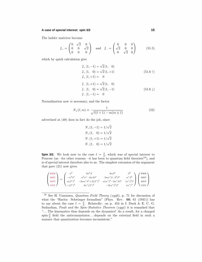
The ladder matrices become

J+ =

0

√2 0

0 0√

20 0 0

and J− =

0 0 0√

2 0 00√

2 0

(51.5)

which by quick calculation give

J+ |1,−1) =√

2 |1, 0)

J+ |1, 0) =√

2 |1,+1) (51.6 ↑)J+ |1,+1) = 0

J− |1,+1) =√

2 |1, 0)

J− |1, 0) =√

2 |1,−1) (51.6 ↓)J− |1,−1) = 0

Normalization now is necessary, and the factor

N±(#,m) ≡ 1√#(# + 1)−m(m± 1)

(52)

advertised at (48) does in fact do the job, since

N+(1,−1) = 1/√

2

N+(1, 0) = 1/√

2

N−(1,+1) = 1/√

2

N−(1, 0) = 1/√

2

Spin 3/2. We look now to the case # = 32 , which was of special interest to

Penrose (as—for other reasons—it has been to quantum field theorists18), andis of special interest therefore also to us. The simplest extension of the argumentthat gave (21) now gives

uuuuuvuvvvvv

=

α3 3α2β 3αβ2 β3

−α2β∗ α2α∗−2αββ∗ 2αα∗β−β2β∗ α∗β2

α(β∗)2 −2αα∗β∗+β(β∗)2 α(α∗)2−2α∗ββ∗ (α∗)2β

−(β∗)3 3α∗(β∗)2 −3(α∗)2β∗ (α∗)3

uuuuuvuvvvvv

18 See H. Umezawa, Quantum Field Theory (), p. 71 for discussion ofwhat the “Rarita– Schwinger formalism” (Phys. Rev. 60, 61 (1941)) hasto say about the case # = 3

2 . Relatedly: on p. 454 in I. Duck & E. C. G.Sudarshan, Pauli and the Spin–Statistics Theorem () it is remarked that“. . .The kinematics thus depends on the dynamics! As a result, for a chargedspin- 3

2 field the anticommutator. . .depends on the external field in such amanner that quantization becomes inconsistent.”

16 Spin matrices

which we agree to abbreviate

ζ( 32 ) = Q( 3

2 )ζ( 32 )

Write

(u∗u + v∗v)3 = (uuu)∗(uuu) + 3(uuv)∗(uuv) + 3(uvv)∗(uvv) + (vvv)∗(vvv)

= ζt( 32 ) G( 3

2 ) ζ( 32 )

G( 32 ) ≡

1 0 0 00 3 0 00 0 3 00 0 0 1

Define

ξ( 32 ) ≡

√G ζ( 3

2 ) with√

G =

1 0 0 00√

3 0 00 0

√3 0

0 0 0 1

Then the left side of

ξt( 32 )ξ( 3

2 ) = (u∗u + v∗v)3 =[ξt( 1

2 )ξ( 12 )

]3is invariant under under the induced transformation

ξ( 32 ) �−→ ξ( 3

2 ) ≡ S( 32 ) ξ( 3

2 ) (53.1)

S( 32 ) ≡ G+ 1

2 ·Q( 32 ) ·G− 1

2 (53.2)

Mathematica informs us—now not at all to our surprise—that the 4×4 matrix

S( 32 ) =

α3 √3α2β

√3αβ2 β3

−√

3α2β∗ α2α∗−2αββ∗ 2αα∗β−β2β∗ √3α∗β2

√3α(β∗)2 −2αα∗β∗+β(β∗)2 α(α∗)2−2α∗ββ∗ √

3(α∗)2β

−(β∗)3√

3α∗(β∗)2 −√

3(α∗)2β∗ (α∗)3

(54)

is unitary and unimodular:

St( 32 ) S( 3

2 ) = I and det S( 32 ) = 1 (55)

Drawing again upon (28) we in leading order have

S( 32 ) =

α3 √3β 0 0

−√

3β∗ α2α∗ 2β 0

0 −2β∗ α(α∗)2√

3β

0 0 −√

3β∗ (α∗)3

+ · · ·

which becomes

S( 32 ) = I + i δθ ·

(k1σσ1( 3

2 ) + k2σσ2( 32 ) + k3σσ3( 3

2 ))

+ · · · (56)

A case of special interest: spin 3/2 17

with

σσ1( 32 ) ≡

0 +√

3 0 0√3 0 +2 0

0 2 0 +√

30 0

√3 0

σσ2( 32 ) ≡ i

0 −√

3 0 0√3 0 −2 0

0 2 0 −√

30 0

√3 0

σσ3( 32 ) ≡

3 0 0 00 1 0 00 0 −1 00 0 0 −3

(57)

By quick computation we verify that (compare (38))[σσ1(

32 ) , σσ2(

32 )

]= 2iσσ3(

32 )[

σσ2(32 ) , σσ3(

32 )

]= 2iσσ1(

32 )[

σσ3(32 ) , σσ1(

32 )

]= 2iσσ2(

32 )

(58)

and find that (compare (39))

σσ21( 3

2 ) + σσ22( 3

2 ) + σσ23( 3

2 ) = 15

1 0 0 00 1 0 00 0 1 00 0 0 1

(59)

Thus are we led by (49: = 1) to the spin matrices

J1( 32 ) ≡ 1

2

0 +√

3 0 0√3 0 +2 0

0 2 0 +√

30 0

√3 0

J2( 32 ) ≡ i 1

2

0 −√

3 0 0√3 0 −2 0

0 2 0 −√

30 0

√3 0

J3( 32 ) ≡

32 0 0 00 1

2 0 00 0 − 1

2 00 0 0 − 3

2

(60.1)

which give

J2( 32 ) ≡ J2

1(32 ) + J2

2(32 ) + J2

3(32 ) = 15

4

1 0 0 00 1 0 00 0 1 00 0 0 1

(60.2)

154 = 3

2

(32 + 1

)(60.3)

18 Spin matrices

All 4-vectors are eigenvectors of J2( 32 ). To resolve that universal degeneracy

we select J3(32 ) which, because it is diagonal, has obvious spectral properties:


2 ) ≡

1000


2 ) ≡

0100


2 ) ≡

0010


2 ) ≡

0001

(60.4)

J1(32 ) and J2(

32 ) have spectra identical to that of J3(

32 ), but distinct sets of

eigenvectors. The ladder operators (45) become non-hermitian ladder matrices

J+( 32 ) =

0√

3 0 00 0 2 00 0 0

√3

0 0 0 0

and J−( 3

2 ) =

0 0 0 0√3 0 0 0

0 2 0 00 0

√3 0

(60.5)

By inspection we have

J+( 32 ) | 32 ,− 3

2 ) =√

3 | 32 ,− 12 ) with N( 3

2 ,− 32 ) = 1/

√3

J+( 32 ) | 32 ,− 1

2 ) = 2 | 32 ,+ 12 ) with N( 3

2 ,− 12 ) = 1/2

J+( 32 ) | 32 ,+ 1

2 ) =√

3 | 32 ,+ 32 ) with N( 3

2 ,+12 ) = 1/

√3

J+( 32 ) | 32 ,+ 3

2 ) = 0

(60.6 ↑)

and similar equations describing the step-down action of J−( 32 ). Matrices

identical to (60.1) and (60.5) appear on p. 203 of Schiff and p. 345 of Powell &Crasemann.7

Spin 2. The pattern of the argument—which I have reviewed in ploddingdetail—remains unchanged, so I will be content to record only the most salientparticulars. We look to the (19)-induced transformation of

ζ(2) ≡

uuuuuuuvuuvvuvvvvvvv

Spin 2 19

and obtain ζ(2) = Q(2)ζ(2) where Q(2) is a 5× 5 mess. From

(u∗u + v∗v)4 = ζt(2) G(2) ζ(2)

G(2) ≡

1 0 0 0 00 4 0 0 00 0 6 0 00 0 0 4 00 0 0 0 1

we are led to write

ξ(2) ≡√

G ζ(2) with√

G =

1 0 0 0 00√

4 0 0 00 0

√6 0 0

0 0 0√

4 00 0 0 0 1

giving

ξ(2) �−→ ξ(2) ≡ S(2) ξ(2)

S(2) ≡ G+ 12 ·Q(2) ·G− 1

2

where S(2) is again a patterned mess (Mathematica assures us that S(2) isunitary and unimodular) which, however, simplifies markedly in leading order:

S(2) =

α4 2β 0 0 0

−2β∗ α3α∗ √6β 0 0

0 −√

6β∗ α2(α∗)2√

6β 0

0 0 −√

6β∗ α(α∗)3 2β

0 0 0 −2β∗ (α∗)4

+ · · ·

= I + i

4k3 2(k1−ik2) 0 0 0

2(k1+ik2) 2k3√

6(k1−ik2) 0 0

0√

6(k1+ik2) 0√

6(k1−ik2) 0

0 0√

6(k1+ik2) −2k3 2(k1−ik2)

0 0 0 2(k1+ik2) −4k3

+ · · ·

From this information we extract the information reported on the next page:

20 Spin matrices

J1(2) = 12

0 +2 0 0 0

2 0 +√

6 0 0

0√

6 0 +√

6 0

0 0√

6 0 +2

0 0 0 2 0

J2(2) = i 12

0 −2 0 0 0

2 0 −√

6 0 0

0√

6 0 −√

6 0

0 0√

6 0 −2

0 0 0 2 0

J3(2) =

2 0 0 0 0

0 1 0 0 0

0 0 0 0 0

0 0 0 −1 0

0 0 0 0 −2

(61.1)

J21(2) + J2

2(2) + J23(2) =6 I (61.2)

6 = 2(2 + 1) (61.3)

The ladder matrices become

J+(2) =

0 2 0 0 0

0 0√

6 0 0

0 0 0√

6 0

0 0 0 0 2

0 0 0 0 0

and J−(2) =

0 0 0 0 0

2 0 0 0 0

0√

6 0 0 0

0 0√

6 0 0

0 0 0 2 0

(61.5)

in which connection we notice that

N+(2,+2) =∞N+(2,+1) = 1/2

N+(2, 0) = 1/√

6

N+(2,−1) = 1/√

6N+(2,−2) = 1/2

N−(2,+2) = 1/2

N−(2,+1) = 1/√

6

N−(2, 0) = 1/√

6N−(2,−1) = 1/2N−(2,−2) =∞

Extrapolation to the general case. The method just reviewed, as it relates to thecase # = 2, can in principle be extended to arbitrary #, but the labor increasesas #2. The results in hand are, however, so highly patterned and so simple thatone can readily guess the design of

{J1(#), J2(#), J3(#)

}, and then busy oneself

demonstrating that one’s guess is actually correct. I illustrate how one mightproceed in the case # = 5

2 .

Arbitrary spin 21

We expect in any event to have

J3(52 ) =

52

32

12− 1

2− 3

2− 5

2

(62.1)

where (as henceforth) the omitted matrix elements are 0’s. And we guess thatJ1(

52 ) and J2(

52 ) are of the designs

J1(52 ) = 1

2

0 +aa 0 +b

b 0 +cc 0 +d

d 0 +ee 0

J2(52 ) = i 1

2

0 −aa 0 −b

b 0 −cc 0 −d

d 0 −ee 0

To achieve J1 J2 − J2 J1 = i J3 we ask Mathematica to solve the equations

12

(a2

)= + 5

2

12

(b2 − a2

)= + 3

2

12

(c2 − b2

)= + 1

2

12

(d2 − c2

)= − 1

2

12

(e2 − d2

)= − 3

2

12

(− e2

)= − 5

2

and are informed thata = ±

√5

b = ±√

8

c = ±√

9

d = ±√

8

e = ±√

5

where the signs are independently specifiable. Take all signs to be positive (anyof the 25 − 1 = 31 alternative sign assignments would, however, work just as

22 Spin matrices

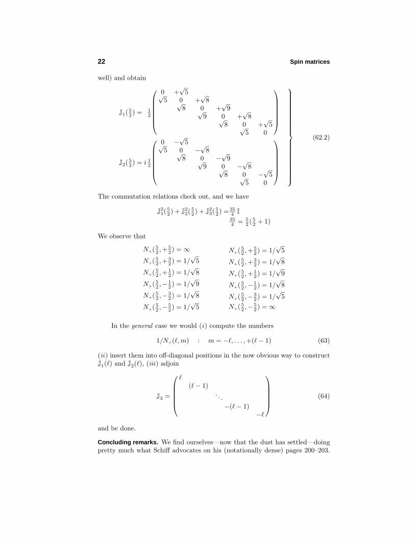
well) and obtain

J1(52 ) = 1

2

0 +√

5√5 0 +

√8√

8 0 +√

9√9 0 +

√8√

8 0 +√

5√5 0

J2(52 ) = i 1

2

0 −√

5√5 0 −

√8√

8 0 −√

9√9 0 −

√8√

8 0 −√

5√5 0

(62.2)

The commutation relations check out, and we have

J21(

52 ) + J2

2(52 ) + J2

3(52 ) = 35

4 I

354 = 5

2 ( 52 + 1)

We observe that

N+( 52 ,+

52 ) =∞

N+( 52 ,+

32 ) = 1/

√5

N+( 52 ,+

12 ) = 1/

√8

N+( 52 ,− 1

2 ) = 1/√

9

N+( 52 ,− 3

2 ) = 1/√

8

N+( 52 ,− 5

2 ) = 1/√

5

N+( 52 ,+

52 ) = 1/

√5

N+( 52 ,+

32 ) = 1/

√8

N+( 52 ,+

12 ) = 1/

√9

N+( 52 ,− 1

2 ) = 1/√

8

N+( 52 ,− 3

2 ) = 1/√

5N+( 5

2 ,− 52 ) =∞

In the general case we would (i) compute the numbers

1/N+(#,m) : m = −#, . . . ,+(#− 1) (63)

(ii) insert them into off-diagonal positions in the now obvious way to constructJ1(#) and J2(#), (iii) adjoin

J3 =

#(#− 1)

. . .−(#− 1)

−#

(64)

and be done.

Concluding remarks. We find ourselves—now that the dust has settled—doingpretty much what Schiff advocates on his (notationally dense) pages 200–203.

Conclusion 23

David Griffiths reports in conversation that he himself proceeds in a mannerthat he considers to be “non-standard” (though it is the method advocated byPowell & Crasemann in their §10–4): he takes the descriptions (64) and (52)of J3 and N±(#,m) to be given; constructs J± matrices that, on the pattern of(51.6) and (60.6), do their intended work; assembles

J1 = 12

(J+ + J−

)J2 = −i 1

2

(J+ − J−

)The merit (such as it is) of my own approach lies in the fact that it

is “constructive;” it draws explicit attention to the circumstance that the(2#+1)×(2#+1) unimodular unitary matrices S(#)—elements of SU(2#+1)—which supply the (2# + 1)-spinor representation of O(3) act upon

ξ =

ξ0ξ1...ξn...

ξ2�

in such a way that

ξn transforms like√(

2�n

)· u2�−n vn : n = 0, 1, . . . , 2#

under (17).

What has any of this to do with “Majorana’s method”? That is a questionto which I turn in Part B of this short series of essays, to which I have giventhe collective title aspects of the mathematics of spin.

SPIN MATRICES FOR ARBITRARY SPIN - Reed College › physics › faculty › wheeler... · 4 Spin...

Documents

Transcript of SPIN MATRICES FOR ARBITRARY SPIN - Reed College › physics › faculty › wheeler... · 4 Spin...