AN EVALUATION OF IMPACT OF MONETARY POLICY ON

ECONOMY OF PAKISTAN

AFTAB ANWAR

06-arid-1435

Department of Economics and Agriculture Economics

Faculty of Sciences

Pir Mehr Ali Shah

Arid Agriculture University Rawalpindi

Pakistan

2015

AN EVALUATION OF IMPACT OF MONETARY POLICY ON

ECONOMY OF PAKISTAN

by

AFTAB ANWAR

(06-arid-1435)

A thesis submitted in partial fulfillment of

the requirements for the degree of

Doctor of Philosophy

In

Economics

Department of Economics and Agriculture Economics

Faculty of Sciences

Pir Mehr Ali Shah

Arid Agriculture University Rawalpindi

Pakistan

2015

iii

CERTIFICATION

I hereby undertake that this research is an original and no part of this thesis

falls under plagiarism, if found otherwise, at any stage, I will be responsible for the

consequences.

Student’s Name: Aftab Anwar Signature: __________________

Registration No: 06 - arid - 1435 Date: ______________________

Certified that the contents and form of thesis entitled “An Evaluation of

Impact of Monetary Policy on Economy of Pakistan” submitted by Mr. Aftab

Anwar have been found satisfactory for the requirement of the degree.

Supervisor: _____________________________

(Dr. Abdul Qayyum Mohsin)

Member: _____________________________

(Dr. Abdul Saboor)

Member: ____________________________

(Dr. Rauf-i-Azam)

Chairperson: ____________________________

Dean: __________________________________

Director, Advanced Studies: ___________________________________

iv

To My Parents,

For

Their Unconditional Love

To My Wife,

For

Her Eternal Encouragement and Support

And

To My Beloved Daughter

v

CONTENTS

Page

List of Tables ix

List of Figures x

Acknowledgements xii

ABSTRACT xiii

1 INTRODUCTION 1

1.1 MONETAERY POLICY 1

1.2 CHANNELS OF MONETARY POLICY 2

1.3 EFFECTIVENESS OF MONETARY POLICY 5

1.4 MONETARY POLICY OF PAKISTAN 12

1.5 RATIONALE OF STUDY 15

1.6 RESEARCH QUESTIONS 15

1.7 THE PURPOSE OF STUDY 16

1.8 FOCUS OF STUDY 16

1.9 THE SCOPE OF THE STUDY 16

1.10 THE OBJECTIVES OF THE STUDY 17

1.10.1 Primary Objective 17

1.10.2 Secondary Objectives 17

2 REVIEW OF LITERATURE 18

2.1 MONETARY EFFECTS FROM RICARDO TO KEYNES 18

2.1.1 Ricardo and Early Classicals 21

2.1.2 J. S. Mill and Marx: The Mid Nineteenth Century 21

2.1.3 The Neoclassical of the Late Nineteenth Century 24

vi

2.1.4 The Innovation of Wicksell 25

2.1.5 Keynes of the Treatise 27

2.1.6 Keynes of the General Theory 31

2.2 MONETARY VARIABLES IN GROWTH THEORY 33

2.2.1 Growth Theory in the Early Twentieth Century 34

2.2.2 Monetary Models Inspired by Financial Repression 34

2.3 POST KEYNESIAN MONETARY THEORY 35

2.3.1 Money and the Real Economy 36

2.3.2 Post Keynesian Views on Interest Rate 38

2.3.3 Monetary Equilibrium and Effective Demand 40

2.3.4 Monetary Policy Variables 42

2.4 CREDIT STRUCTURE IN MONETARY TRANSMOSSION 44

2.5 MONETARY POLICY OBJECTIVES 46

2.6 EFFECTIVENESS OF MONETARY POLICY 46

3 MATERIALS AND METHODS 58

3.1 DATA SOURCES 58

3.2 EMPIRICAL ESTIMATION OF DATA 58

3.3 VARIABLES OF THE STUDY 59

3.4 HYPOTHESIS OF THE STUDY 59

3.5 MODEL OF STUDY 61

3.6 RESEARCH METHODOLOGY 64

3.6.1 Unit Root Test 67

3.6.2 Error Correction Mechanism 70

3.6.3 Granger Causality Test 71

vii

3.6.4 Homoskedasticity 73

3.6.5 Standardized Coefficient Technique 73

3.6.6 Multicollinearity 74

3.6.7 Autocorrelation or Serial Correlation 75

4 RESULTS AND DISCUSSION 78

4.1 IMPACT OF MONETARY POLICY VARIABLES AND CPI

INFLATION IN GDP GROWTH RATE

78

4.2 IMPACT OF MONETARY POLICY ON ECONOMIC GROWTH IN

CASE OF BROAD MONEY

82

4.3 IMPACT OF PREVIOUS PERIOD MONEY SUPPLY ON CURRENT

MONEY SUPPLY

86

4.4 IMPACT OF MONETARY POLICY AND CPI INFLATION TO

REDUCE UNEMPLOYMENT

87

4.5 IMPACT OF MONEY SUPPLY AND RATE OF INTEREST ON

EXCHANGE RATE

89

4.6 IMPACT OF MONETARY POLICY TO REDUCE INFLATION 92

4.7 GDP GROWTH RATE, GROSS SAVING AND TOTAL

CONSUMPTION EXPENDITURES

93

SUMMARY 98

CONCLUSION 99

FUTURE VISION 101

RECOMMENDATIONS 102

LITERATURE CITED 107

APPENDICES 118

viii

ABBREVIATIONS

ADF: Augmented Dickey Fuller

AEG: Augmented Engle Granger

ARIMA: Autoregressive Integrated Moving Average

BLUE: Best Linear Unbiased Estimator

CPI: Consumer Price Index

CLRM: Classical Linear Regression Model

ECM: Error Correction Model

EG: Engle Granger

GDP: Gross Domestic Product

IT: Inflation Targeting

KPSS: Kwiatkowski-Phillips-Schmidt-Shin

MD: Demand for Money

MS: Money Supply

MEC: Marginal Efficiency of Capital

MIT: Massachusetts Institute of Technology

NAIRU: Non-Accelerating Inflation Rate of Unemployment

OMOs: Open Market Operations

OLS: Ordinary Least Square

RAND: Research and Development

SBP: State Bank of Pakistan

VAR: Vector Autoregressive

WPI: Wholesale Price Index

ix

LIST OF TABLES

Table No. Page

1 Economic Growth, Monetary Policy Variables and CPI Inflation 79

2 Correlation Matrix of Study Variables 79

3 Impact of Monetary Policy on Economic Growth in case of

Broad Money

81

4 Current Period Money Supply and Previous Period Money

Supply

81

5 Correlation Matrix of Current Money Supply and Previous

Money Supply

88

6 Monetary Policy, CPI Inflation and Unemployment 88

7 Money Supply, Rate of Interest and Exchange Rate 91

8 Monetary Policy and CPI Inflation 91

9 Gross Saving and GDP Growth Rate 95

10 Total Consumption Expenditures and GDP Growth Rate 95

x

LIST OF FIGURES

Figure No. Page

1 Monetary Policy Transmission Mechanism 3

2 Liquidity Trap and Money Market 7

3 The Classical Case and Money Market 7

4 Flow Chart of Study 77

5 Scatter Diagram of Real GDP Growth Rate with Straight Line 84

6 Scatter Diagram of CPI Inflation with Straight Line 84

7 Scatter Diagram of Real Discount Rate with Straight Line 84

8 Scatter Diagram of Real Exchange Rate with Straight Line 85

9 Scatter Diagram of Broad Money M2 with Straight Line 85

10 Combine Historigram of GDP Growth Rate, Real Exchange Rate,

Real Discount Rate, Average CPI Inflation and Unemployment

Rate

85

11 Scatter Diagram of Unemployment Rate with Straight Line 96

12 Scatter Diagram of Gross Saving with Straight Line 96

13 Scatter Diagram of Total Consumption Expenditures with Straight

Line

97

14 Combine Historigram of GDP Growth Rate, Gross Saving and

Total Consumption Expenditures

97

15 Filled Radar Diagram of Real GDP Growth Rate for Annual and

Quarterly Data

103

16 Filled Radar Diagram of Average CPI Inflation for Annual and

Quarterly Data

103

xi

17 Filled Radar Diagram of Broad Money for Annual and Quarterly

Data

104

18 Filled Radar Diagram of Unemployment Rate for Annual and

Quarterly Data

104

19 Filled Radar Diagram of Real Discount Rate for Annual and

Quarterly Data

105

20 Filled Radar Diagram of Real Exchange Rate for Annual and

Quarterly Data

105

21 Filled Radar Diagram of Total Consumption Expenditures for

Annual and Quarterly Data

106

22 Filled Radar Diagram of Gross Saving for Annual and Quarterly

Data

106

xii

ACKNOWLEDGEMENTS

First I pay my humble thanks to Almighty Allah who knows all the things which

pass through our hearts, who gave me the courage to complete this manuscript. I

also offer my most humble thanks to Hazrat Muhammad (May peace of Allah be

Upon Him and his descendants), who made us aware of our creator and guided us

to the track which leads to the success, who is symbol of love and affection for all

the creatures of Allah.

My profound gratitude first goes to my supervisor Dr. A. Q. Mohsin for being an

excellent coach in guiding me through this thesis. I sincerely acknowledge his

rigorous commitment and generous time to ensure the quality of this thesis as well

as the timely completion. In addition, the principles and the values I learned from

him would be an inspiration in my life.

I would like to show my greatest appreciation to Prof. Dr. Abdul Saboor,

Chairman Department of Economics and Agricultural Economics. I cannot say

thank you enough his tremendous support and help. I feel motivated and

encouraged every time attended his meeting. Without his encouragement and

guidance this dissertation would not completed.

I have nobility to express my deep sense of gratitude and indebtedness to Dr.

Rauf-i-Azam, Director University Institute of Management Sciences for his

sincere cooperation during the study. I offer special thanks to Higher Education

Commission which made this study possible through their financial support.

Without their concern, I would not have been able to undertake this study.

While I am solely responsible for this study, It would be remiss of me not to

acknowledge the support and encouragement of all friends, colleagues and relatives

who stood by me when frustration escalated and the going got mighty tough.

Thanks are extended to Muhammad Aamir Khan, a caring friend, for reducing

the pain endured in completing this study; thanks for the engaging intellectual

interaction; and thanks for the distinguished editorial help.

These lines provided me an opportunity to rightly acknowledge the unmatched

personalities of my affectionate parents and family for their inspiration,

encouragement and prayers for my success and prosperities in all walks of life.

May Allah Bless all these noble personalities, AMEEN

(AFTAB ANWAR)

xiii

ABSTRACT

Objective of the study is to evaluate the impact of monetary policy on the

economy of Pakistan in the light of Monetarist and Keynesian views. Keynesian

argue that monetary policy is ineffective in stimulating the economic growth of a

country, which is said to be determined by the economic growth levels of its large

and developed trading partners. Money supply and inflation are considered to be

insignificantly related to economic growth. It is further argued that the monetary

authorities cannot control money supply changes as desired, namely, to keep them

within the set money supply guidelines, because of foreign external forces flowing

out of international trade conducted with these large and developed partners. By

contrast, the monetarist counter-argument affirms the efficacy of the money supply

and inflation in influencing the economic growth of a country. Monetary

authorities are said to be capable of controlling money supply via the bank rate

(repo rate), that the current level of money supply is significantly related to that of

the previous period. By using forty year data, it is evaluated that impact of interest

rate on economic growth is negative and at the same time its impact on

unemployment is positive. It is also investigated that there exist tradeoff between

inflation and unemployment. It is also estimated that current money supply

strongly depends upon the money supply of previous period. Impact of monetary

base and broad money on economic growth and on unemployment is very much

weak near to zero. Saving is the component of aggregate savings and consumption

is the necessary component of aggregate demand but it is evaluated that impact of

saving on GDP growth rate is significantly positive as compare to consumption. So

those policies should be used which are helpful to increase the saving in the

xiv

country. In the case study of Pakistan, the empirical findings confirm that the

economic growth is not significantly related to changes in money supply and

inflation but it is significantly related to the changes in real exchange rate and

interest rate and that ability of monetary authorities to control money supply is

constrained by external factors. While monetary policy is ineffective in controlling

changes in the money supply, keeping it within set target limits or guidelines, it is

able to influence the current level money supply by operating on that of the

previous period.The Keynesian argument that the monetary authorities cannot

control money supply changes, i.e. keeping them within set target guidelines, is

confirmed. The basis of this argument is said to be the unfair terms of trade faced

in dealing with large and developed countries. This is despite the significant

relationship between the current level of money supply and that of the previous

period.

1

Chapter 1

INTRODUCTION

1.1 MONETARY POLICY

To maintain the price stability, central bank of any country tries to control

the money supply of that country. Therefore, monetary policy plays its role to

stabilize the economic growth through the number of channels. Price stability is

major contribution of monetary policy for sustainable growth of a country. As it is

considered that continuous rise in price level is only due to monetary phenomenon,

so for maintaining the price stability monetary policy uses different tools to effect

the money supply. Empirical evidence of economic literature recommends that low

price level and sustainable long run growth are closely related to each other. Only

the costs are not affected by the monetary policy but it has comprehensive impact

on economy’s financing conditions. It also affects the credit’s availability and

willingness of banks to assume the risks etc. Future expectations about economic

activities, inflation, exchange rate, investment and consumption are also affected

by the monetary policy.

If monetary authorities decide to cut the interest rate then in the result, the

investment activities and expenditures on durable goods will increase. Currency

depreciation is also the result of low interest rates because in case of more

expensive imported goods, the demand for domestic goods rises. Due to all these

causes unemployment will reduce but output, consumer expenditure and

investment will rise.

2

1.2 CHANNELS OF MONETARY POLICY

Important channels of monetary policy which make it more effective to

meet the economic targets are interest rate channel, credit channel and assets price

channel. These channels are not alternative to each other but they can be operated

simultaneously.

Interest rate channel is also known as workbook channel. Change in interest

rate effect the cost of borrowing and capital. Consumption and investment both are

affected by the direct impact of interest rate. From central bank to banks during the

transmission process of monetary policy it is not fitting for macroeconomic time

arrangement to recognize the credit channel from money channel in light of the fact

that credit channel works through the benefits of the banks inasmuch as money

channels works through banks liabilities. There exist close relation between assets

and liabilities by accounting identities. Macroeconomic studies recommend that

fluctuations in output and price in light of progress in the advance quantities and

deposits are rarely conclusive (Bernanke and Blinder, 1992).

To check the importance of credit channel most credible studies have

utilized the microeconomic information and have inspected the distinction in the

middle of banks and firms in monetary policy as indicated by their size and

specific. It is noted that little firms confront more liquidity requirements and for

financing little firms relies on upon banks. On the other side little banks confronts

trouble to issue the advances on the grounds that little banks can't utilize bond

possessions as a shock absorber (Kashyap et al., 1993).

3

Figure: 1 Monetary policy transmission mechanisms

POLICY RATE

Bank and Market Interest Rates

Expectations

Money

Supply

Asset

Prices Lending Volume

Exchange

Rate

Interest

Rate

Channel

Exchange

Rate Channel

Wealth

Channel

Credit

Channel

Supply and Demand on the

Goods and Labour Markets

Import Prices

Domestic Prices

Price Developments

Wage and

Price Formation

4

Credit channel is one of the important channels of monetary policy to

depress the economic activities. In this channel, by utilizing low bank lending

contractionary impacts of monetary policy are transmitted to a vast degree. In small

and open economy exchange rate channel is also a crucial one. The monetary

tightening causes the nominal exchange rate to increase. Due to nominal strictness

prices remain constant in small time period and in the result we see the

appreciation in real exchange rate (Mishkin, 1996).

Lastly asset prices like equity prices, houses price and forex rate also play

their role for the transmission of monetary policy to economic activity. Whenever

monetary policy affect the external value of country’s currencies to open the

potential across countries for different effects then it means that exchange rate

channel is in action.

Any rise in the currency rate by keeping other things as constant will lead to

an appreciation. In the consequence of appreciation not just the import costs

including import of middle merchandise and materials will diminished however

this will end in the misfortune of intensity for exporters and import-contending

firms. Improvement in the term of trade due to currency appreciation, will involve

only in growth of real income, but on the other side output and employment will

decrease due to competitiveness effects (McLennan et al., 1998).

Central bank of any country conducts the monetary policy to minimize the

economic fluctuations and to keep low inflation. Monetary policy effects the

5

financial and economic decisions of the people. For example the decisions about

the loan for new business, to buy a new car or house, to invest in a new business or

put money in banks, bonds etc are affected by the monetary policy. To formulate

the monetary policy central banks focus primarily on the economic condition of the

country. However,other than the national economic conditions, central banks must

consider the regional economic conditions. In case of measuring the effects of

monetary policy, focus is on national level variables. As we know that there is lot

of difference in regional and state economic conditions so it is impossible to say

that impact of monetary policy would be same across different regions and states.

About 50 year ago founder of the Regional Science Foundation, Walter Isard,

stated that “since each of the nation’s regions has different resource potential and

confronts obstacles to growth, it follows that monetary policies alone generate both

retarding factors for some regions and problem intensifying factors other regions”.

It is important for each member of the nation to understand that how much their

region or state will be affected by the changes in the monetary policy (Han, 2012).

1.3 EFFECTIVENESS OF MONETARY POLICY

Discussion on the effectiveness of monetary policy is still going on between

Keynesian and monetarists. During the great depression (1929-33) with the

increase in money supply, income level of the people did not change and in the

result all this situation sparked the Keynesian view about monetary policy and from

Keynesian school of thought some extremists argued that to stimulate the economy

“money does not matter”. According to monetarist economists led by Milton

Friedman monetary policy is an effective tool to stimulate the economy, thus

6

“money matter”. Controversy about monetary policy is remained unsettled (Mohr

and Fourie, 2007).

According to Keynesian there is very weak relationship between monetary

sector and real sector. Conversely crucial element of interest rate is suggested as an

indirect link between both the sectors to connect the changes in money supply and

economic activities and all of this happen in two stages. In the first stage with

prevailing interest rate any rise in money supply (Ms) above the demand for money

(Md) causes an excess money supply (Ms > Md) and in the result demand for

other financial assets like bonds increases and prices of these assets will rise and all

this lead to drop in interest rate (i). In second stage decline in interest become the

cause of increase in the aggregate demand via an in crease in investment (I).

Consequently country Gross Domestic Product increases

i.e., If Ms↑ → (Ms > Md) →↑prices of other financial assets → ↓i → ↑I → ↑GDP

By implication if due to increase in money supply further decline in interest

rate is impossible, this situation is called Keynesians liquidity trap and in this

situation money market equilibrium is represented by a horizontal LM curve. In

liquidity trap situation money market is interest in-elastic and people are indifferent

between holding money and financial instruments.

In this case increase in economic growth is possible through the movement

in IS curve via fiscal policy. On the other side according to monetarist monetary

transmission

7

Figure: 2 Liquidity trap and money market (SOURCE: Dornbusch et al. 2004)

Figure: 3 The classical case and money market (SOURCE: Dornbusch et al. 2004)

8

mechanism is to be direct and for this purpose they take the Irvin Fisher equation of

exchange that is MV = PQ

Where M is quantity of money, V is velocity of money, P is average price level and

Q is real value of goods and services.

Now with constant V, any change in quantity of money M result in equi-

proportional change in total output PQ which is called direct monetary transmission

mechanism because in this way any change in money supply directly effect the

economy.

Against the Keynesian approach of horizontal LM curve due to liquidity

trap, Monetarist considers a vertical LM curve that is called classical case. In this

case any increase in government spending does not affect the level of income and

lift up only the interest rate. Fiscal policy has no impact on the equilibrium of the

economy and monetary policy has maximum effect. Increasing interest rate crowds

out an amount of private spending equal to the increase in the government

spending.

The economic issue tended to in this study streams straightforwardly from

the Keynesian and Monetarist verbal confrontation laid out above. Though

Keynesians consider the monetary transmission mechanism to be indirect, while

monetarists respect it to be direct, the stress is sort of moved on account of the

issue under examination. The center in this study is on whether monetary policy

through the transmission mechanism can strengthen the economic growth of a little

9

and open economy. In the same way that the Keynesian revolution occurred as a

consequence of the ineffectualness of monetary policy throughout the Great

Depression, the disappointment of the business sector economy to address the

socio-economic issues in Latin America started an economic school of thought

called structuralism. The structuralist hypothesis, otherwise called the Latin

American School of Development, created as an option to what was viewed as the

disappointment of orthodox economics, alluded to as neo-progressivism by

structuralists. The Latin American countries, which were experiencing socio-

political conversion, made minimal economic advancement. These countries

started to address the reliance of their developing economies on those of huge

created western economies, which are said to profit at the cost of the little

developing countries with which they exchange. The structuralist hypothesis is

focused around the conviction that the issues of little economies exchanging with

substantial created economies are structural instead of economic. As needs be,

markets are questioned and disfavoured by structuralists, who rather advocate

government mediation (Khabo, 2002).

Rising liberation assessments fought that substantial and created western

countries devastated those little and developing countries with which they traded.

Domestic monetary policy is accordingly said to be insufficient, on the grounds

that the economic growth issue confronted is not monetary yet structural (Bruce

1980).

Objectives of monetary policy are price stability, progressive economic

growth, achievement of full employment, smoothness of business cycle, prevention

10

of financial crises and maintaining the long run interest rates and exchange rates.

No doubt some objectives are consistent with others, as objective of price stability

often conflict with the interest rate stability. In this case country can assign equal

weight to the objective or can put greater weight to one objective as compare to

other. Monetary policy targets can be classified as intermediate targets or operating

targets. Intermediate targets are not controlled by the central bank and these targets

are variables that affect the objectives of monetary policy such as monetary

aggregates and long term interest rates.

On the other side operating targets are short run goals of central bank. To

affect intermediate targets central bank use monetary policy instruments like

reserve money and short run interest rate. Monetary instruments are of two types

such that direct and indirect. Direct instruments function according to regulations

of central bank that directly effect the interest rate or volume of credit and these

direct instruments become ineffective in case of developed money and financial

markets. Market based instruments or indirect instruments are of three types such

that open market operations central bank lending policies and reserve requirements

and these are used to inject and absorb liquidity. Other indirect instruments are

central bank obligations and central bank auction of central bank credits (Mohsin,

2010).

Monetary policy regime has very important consequences for the behavior

of domestic variables like output and inflation but for international variables like

current account and real exchange rate it has less importance. Best policy for

11

central bank is to focus on targeting the domestic inflation. It is also being noted

that exchange rate system should be flexible because high valued currencies are not

only inflationary but also become the obstacle in the way of economic growth

(Sulaiman, 2010).

Impact of fiscal policy on economic growth is significant and there is

cointegeration relationship between exchange rate, government expenditures,

inflation, growth and money stock but the of monetary policy variables like

exchange rate and inflation on economic growth is negative. So monetary policy is

not much supportive to uplift the economic growth of any country (Khosravi, A.

and M. S. Karimi. 2010).

In macroeconomics the monetary policy affect on the real economy has been a

divisive zone (Bernanke and Gertler, 1995). Important question is this that whether

changing interest rate has some effect on the variables of real economy and how

much these effects are powerful. This seems to be more important when it stew

down to the regional level seeing as monetary policy naturally address the national

targets whereas we see different structures and characteristics within a monetary

union. Hence it is possible that they might respond in disproportionately to a wish

for of a standardized monetary policy. Some distributional implications, as a

consequence, there will be across the region because by policy any economic

activity may be encouraged in core whereas the periphery may become more

miserable (Ridhwan et al., 2008).

12

1.4 MONETARY POLICY OF PAKISTAN

In Pakistan primary roles of monetary policy are monetary policy

management and financial sector stability. According to State Bank of Pakistan

Act, 1956 monetary policy will be supportive for both the objectives of promoting

the economic growth and price stability. By targeting the monetary aggregates

such that broad money supply growth as an intermediate target and reserve money

as an operational target in accordance with Government real GDP growth and

inflation targets, SBP achieves its goals (Akhtar, 2007).

The Taylor rule (1993) centers just on two objectives: output and inflation

as the rule insist on that central bank should raise the nominal interest rate by more

than one percentage point for one percent increase in inflation but in practice, the

central bank's loss function, particularly in developing countries, holds goals other

than these two, in the same way as the interest rate smoothing, exchange rate

stability, and so on. Variance decay demonstrates that the vast majority of the

variation in the interest rate is explained by its lagged values. Other variables, in

explaining variation in the interest rate, might be positioned as inflation,

government borrowing, exchange rate, output gap, trade deficit and at last foreign

exchange reserves. Result of study confirms that the State Bank of Pakistan does

think about both inflation and output. However the policy has additionally been

centered on different components as the majority of the goals we included in the

estimation altogether influence the conduct of monetary policy instrument. The

imperative result is that the trade deficit that is not taken as monetary policy

objective in the exact writing has critical effect on the central bank (SBP's) actions.

13

Two variables that we have included other than destinations (government

borrowing and foreign exchange reserves) and the exogenous factor (foreign

interest rate) also explain significantly the variation in interest rate. Other

objectives should take into account these other objectives for a country like

Pakistan to modify the Taylor type rule. Basic Taylor rule that concentrates on

inflation and output may be inadequate for the developing countries (Malik, 2007).

For the vast majority of the central banks on the planet, price stability has

turned into the prime target of monetary policy alongside a worry to real

adjustment in the short run. Thus summarizing monetary policy objectives by a loss

function defined over deviations of inflation from target and that of output from

potential level has become a norm in the literature on monetary economics. Yet

monetary policy can settle real monetary movement just in the short run. Allocating

monetary policy the goal of long run growth obliges setting operational focus in

such a path, to the point that real interest rate is dependably beneath neutral interest

rate. Pakistan has encountered cycles in inflation and real budgetary action.

Inflation arrived at its crest of 23 percent in 1974, and touched the most minimal

level of 2.4 percent in 2002. Essentially, the real output gap differed between -7

percent in 2002 and 6.5 percent in 2008. Generally, there has been more focus of

SBP on growth objective as opposed to concentrating on inflation and output gap

(Malik and Ahmed 2007).

During the most recent three decades the perspective has raised that

monetary policy can attain just predetermined number of goals. Utilizing Pakistani

information, this study endeavors to gauge Taylor-type response capacity and its

14

slight altered form characterized over inflation and real GDP growth. Our results

show professional cyclical reaction of SBP to economic fluctuations. Other than

this price stability alongside output stability, economic growth has been given

priority. One of the paramount discoveries of the study is that SBP has been

leading master cyclical policy; however, the level of pro-cyclicality diminished

altogether after money related segment changes. This could have been because of

SBP fixation on policy goals other than inflation and output adjustment. One of

such targets has been discovered to be economic growth. Surprisingly, the level of

master cyclicality towards economic growth has expanded after 1989. Finally, the

study makes inconsistent reaction of SBP to inflation and output deviations from

their separate targets; however policy consistency has enhanced since the start of

this decade. State Bank of Pakistan has picked up self-governance in setting policy

instrument as an after effect of budgetary division changes. The motivation behind

why SBP's reaction has not gotten counter-cyclical could be the center of policy on

targets other than price stability in the long run and real adjustment in the short run.

Other than this, SBP likewise need to withstand regular fiscal pressures which to a

great extent weaken the monetary policy stance and there is a consistent struggle

for keeping up stability of exchange rate. To achieve the target of price stability,

there must be legislation to decrease the fiscal pressure and SBP need to give

careful consideration to this target; otherwise inflationary expectations couldn't be

controlled (Malik and Ahmed, 2011).

In order to untie the issues related to the impact of monetary policy

different studies are conducted. For this purpose Carlino and DeFina (1998, 1999)

15

and Owyang and Wall (2004) have conduct a research on USA economy on the

impact of monetary policy while Ramaswamy and Slok (1998) and Clements et al.

(2001) have studied the impact of monetary policy in European countries. In broad-

spectrum their findings suggest disparity among the output effects in response to a

common policy shock. Some studies have suggested that the output effects in

eurozone are very common (Peersman, 2004). Gerlach and Smets (1995) and

Kieler and Saarenheimo (1998) conclude that there is no variation in the impact of

monetary policy across the countries. All of these findings conclude that there are

still significantly different views on the actual impact of monetary policy.

1.5 RATIONALE OF STUDY

Outstanding growth rate of many developing countries like India, China,

Malaysia, Taiwan and Singapore is big reason for the study motive. On the other

side Pakistan is much behind than its targets. If these developing countries can

manage to grow, then it is also possible for Pakistan to grow as well.

1.6 RESEARCH QUESTIONS

Questions that can create the confusion are as under

Which one is true about the effectiveness of monetary policy, Keynesian or

Monetarist?

How much the monetary policy is effective to stimulate the economic

growth?

Either inflation is always and every where a monetary phenomenon?

How much monetary policy is effective to trim down the unemployment?

16

Whether there exist tradeoff between unemployment and inflation?

These questions are not explored scientifically and comprehensively especially in

case of Pakistan.

1.7 THE PURPOSE OF STUDY

Purpose of study is to design a monetary policy which is non-inflationary

on one side but on other side it is growth supportive and to encourage flexibility of

interest rates to respond to market forces. It is also the purpose of this study to

make a comparison between two opposing views that is, Keynesian and monetarist,

about the monetary policy.

1.8 FOCUS OF THE STUDY

Main focus of this study is to check that either monetary policy can play its

role to stimulate the economy or not in Pakistan and hopefully outcomes of this

study will help most of the developing countries. To know about the basis behind

the poor economic performance of Pakistan, hypotheses are formulated and a study

about the impact of monetary policy is undertaken. Appropriate econometric model

is used for the empirical analysis of Pakistan economy. Recommendations to

achieve the growth through monetary policy are given in conclusion.

1.9 THE SCOPE OF THE STUDY

In term of scope this study is confined to evaluate the impact of monetary

policy to stimulate the economic growth without any analysis of underlying

reasons. Covering period of this study is from 1972 to 2011.

17

1.10 THE OBJECTIVES OF STUDY

Objectives of the study are as under

1.10.1 Primary Objective

To stimulate the economic growth of Pakistan, the prime objective of this

study is to evaluate the impact of monetary policy on economy of Pakistan.

1.10.2 Secondary Objectives

Other objectives of the study are as under

To find out whether or not the current period money supply depends on

money supply of previous period.

To measure the impact of monetary policy variables and CPI inflation on

growth rate of the economy.

To determine the effectiveness of monetary policy to trim down the

unemployment.

To study that impact of money supply and rate of interest on exchange rate.

To estimate the impact of monetary policy on inflation.

To identify the role of saving and consumption for increasing growth rate.

18

Chapter 2

REVIEW OF LITERATURE

2.1 MONETARY EFFECTS FROM RICARDO TO KEYNES

Many ideas and alternative approaches in the sphere of monetary theory

have their antecedents in the theoretical contributions and controversies which

arose in the history of economic thought. Writers such as David Hume and Adam

Smith in the 1700s included as part of their discourse early expressions of the

quantity theory of money, in which the general price level was related to the

quantity of money in circulation. The writings of David Ricardo in the early 1800s

are however generally recognised as a milestone in the comprehensive examination

of economic issues using an analytical framework (Blaug 1996). Ricardo is

recognised for use of the long period as an analytical device in which capital

adjusts through investment between uses in such a way as to equalise the rate of

profit between alternative allocations (Barber 1967). But the Classical1 conception

of money was that of a facilitating fluid behind which real magnitudes were

determined (Dennis 1981). Is there evidence that Ricardo portrayed monetary

variables as having at least some influence on investment? When and through

which economic writers did this connection emerge? These questions are examined

through viewing the writings of prominent economic thinkers over the course of

the nineteenth century, in particular Ricardo, Thornton, John Stuart Mill, Marx,

Marshall, Bohm-Bawerk and Wicksell, relating to monetary influences on

investment. This is of course not an exhaustive list of economic writers making

significant contributions concerning monetary issues over this period. It serves

though to capture the key perceptions and innovations concerning monetary

19

influences on real economic magnitudes over this period.

A crucial distinction in examining monetary theories for the purposes of

this thesis is the distinction between Real Analysis and Monetary Analysis as put

forward by Schumpeter (1954). A monetary theory in the tradition of Real Analysis

may incorporate various monetary variables, but in equilibrium the magnitudes in

the economy are precisely as they would be if only real economy magnitudes were

involved. There is an underlying assumption that all essential features of an

economy can be captured through the interaction of real magnitudes: "Money

enters the picture only in the modest role of a technical device that has been

adopted in order to facilitate transactions." (Schumpeter, 1954). Under the

Monetary Analysis tradition, on the other hand, monetary variables are inextricably

involved in determining real economic magnitudes.

Monetary variables lead to real outcomes which differ from the magnitudes

which would arise if only real magnitudes were determinants. Monetary

phenomena are reflected as persistent forces which combine with real forces in

determining long-period equilibrium positions; they are not confined to transitory

effects. The importance of the distinction in examining the relationship between

monetary variables and investment (a real magnitude in this context) lies in that it

requires a theory with the characteristics of Monetary Analysis to allow the

possibility of such a relationship on a persistent and significant basis within its

theoretical structure. Adoption of a theory in the Real Analysis tradition excludes

the possibility of such a relationship ab initio in view of its underlying

20

assumptions. Blaug (1996) provides a less comprehensive portrayal, though in the

same vein: "By 'monetary analysis', we mean any analysis that introduced the

element of money at the outset of the argument and denies that the essential

features of economic life can be represented by a barter model."

Three strands of particular importance to monetary theory which were

introduced and examined by economic writers in the eighteenth and first half of the

nineteenth centuries, relate to: the quantity theory relationship between money in

circulation and the general price level as well as real economic magnitudes, the

question of whether there is an automatic tendency of an economy to remain at or

return to an aggregate supply–aggregate demand equilibrium level as captured by

Say's Law, and the economic effects of non-commodity money arising through the

bank system, as expressed in the Currency School versus Banking School

alternative viewpoints and debates.

These three strands served as foundation stones on which increasingly

advanced economic analyses were developed through the remainder of the

nineteenth century and most of the twentieth. They remain as underlying

theoretical departure points in alternative schools of thought and approach to

monetary theory to the present. Their origins in classical economics are highlighted

below, especially since they are frequently used, both in this thesis and in writings

on monetary theory in general, to identify the theoretical foundations of alternative

approaches and arguments concerning the economics of money.

21

2.1.1 Ricardo and Early Classicals

Examination of Ricardo's analysis of economic issues suffers the dangers

arising from his work having been so extensively re-cast and re-formulated. It is a

tribute to Ricardo that his analytical method came to form the core of much of

economic teaching for a period of almost seven decades after his death in 1823. But

it is an indication of a great economic conception with many flaws and

inconsistencies that subsequent economists have felt the need to re-examine the

analyses in more clearly formulated and corrected terms, with mathematical

expression that Ricardo himself did not use. Blaug (1996) for instance suggests that

Ricardo operated with three models at different times : "a Pasinetti-type, constant

wage model; a disequilibrium variable-wage model; and a genuine dynamic

equilibrium growth model."

2.1.2 J S Mill and Marx: The Mid Nineteenth Century.

John Stuart Mill's Principles of Political Economy of 1848 draws openly

and fully on the analytical framework of Ricardo in its primary coverage. Mill does

however offer new approaches on various subjects as well as reformulations, and

these do include issues pertaining to money. Contrary to Ricardo, Mill lends some

support to the real bills doctrine and the Law of Reflux as being "far nearer to

being the expression of the whole truth than any form whatever of the currency

theory" (Mill 1848). However, in his more detailed analysis, he accommodates

both a Banking School and Currency School approach by distinguishing a

quiescent and speculative state of the economy. In the quiescent state, referring to a

situation where markets are close to equilibrium and not overheated, the Law of

22

Reflux would be operative and would prevent an over-issue of notes. However, in

the speculative state, corresponding to high relative economic activity, note issue

could expand excessively without being automatically curbed by reflux, even if

banks are cautious enough to follow a 'real bills' doctrine. The note issue could feed

an inflationary spiral, with higher prices leading to still further note issues, in

accordance with the quantity theory and Currency School view (Mill, 1848). As

with the earlier Classicals, in respect of production, Mill was "steadfast in his

defense" of Say's Law (Sowell:1972). J S Mill was acquainted with the work of

Thomas Tooke, whose major book, History of Prices, was first published in 1838

(Makinen 1977).

Increasing interest rates were accompanied by increasing general price

levels, decreasing interest rates by decreasing price levels. Tooke's explanation of

this was that interest rates constitute an input cost for production, so that increasing

interest rates raise production costs which in turn are passed on in the form of

higher prices. Tooke also maintained from his statistical analysis that rises in the

price level generally preceded rises in the quantity of money in circulation rather

than vice versa. These two findings were strong ammunition against the Currency

School view, and it appears that Mill sought to incorporate their consequence in the

monetary theory that he expressed. Adoption of a Banking School viewpoint, even

if only partially, opens up the possibility of a link between money and investment

in Mill.

The Banking School recognised a broad range of financial instruments as

constituting 'money' for analytical purposes in addition to bank notes and gold.

23

Short-term forms of credit such as trade bills, self-liquidating commercial paper

and notes based on goods in process were considered close substitutes for narrowly

defined money, since they were negotiable instruments which could be used to

effect payment, even though they bore a discount or implicit interest rate. These

were the very instruments that could be used directly or indirectly as a vehicle to

finance investment expenditure. Thus both the extent of availability of these

instruments and the effective interest rate at which they could serve to raise funds

could be sources of a causal mechanism between money and investment. Mill did

not however pursue this line of inquiry.

It is noteworthy that the Bank of England had commenced practising

monetary management at the time when Marx was writing. The Bank Charter Act

of 1844 provided a legal framework in which the Bank's discount rate could be

used as an instrument of credit regulation. The Bank did also engage in a form of

open market operations through borrowing against Consols (Blaug 1996). It was

therefore eminently possible that Marx could have explored the possible effects

Marx directly challenged Say's Law and "rejected the necessary equality of supply

and demand (Sowell 1972). He however regarded the interest rate as a purely

monetary phenomenon, with very little connection to rates of profit. He rejected the

notion of a 'natural' rate of interest and did not accept the argument of Thornton

and Ricardo that there is in principle a long period rate of interest which tends to

equality with the long-period yield on real capital. He did maintain that the interest

rate, along with profit rates on physical capital, would have a secular tendency to

decline, but this was as much through the continued concentration of saving in the

24

hands of an expanding banking sector as through falling capital yields as a result of

relentless capital accumulation.

His views were broadly in line with the Banking School, with the Law of

Reflux operating, and monetary usage being determined by the requirements of

commerce. He was explicitly opposed to the quantity theory, possibly regarding it

as contrary to his labour theory of value (Blaug 1996). But with this combination,

he viewed the monetary sector as providers of funds in his analysis of capitalistic

production, rather than regarding money as a significant issue for examination from

a theoretical viewpoint for his purposes. Marx' conception of the workings of a

capitalist economy could possibly be placed in the category of Monetary Analysis

rather than Real Analysis in terms of Schumpeter's distinction (1954), but this

would be somewhat tenuous since he did not consider monetary effects in depth.

2.1.3 The Neoclassical of the late Nineteenth century

The neoclassical economists in the last decades of the nineteenth century

could once again best be categorised in the Real Analysis rather than Monetary

Analysis tradition. These years saw the rapid advancement of the marginalist

approach, applied to utility on the part of consumers and to revenue, costs, capital

productivity and the like on the part of the firm. Walras was one of the discoverers

and initiators of the principle of diminishing marginal utility and its implications,

though he is most closely associated with the system of equations depicting an

economy in general equilibrium which has come to be associated with his name.

25

Bohm-Bawerk, (1888) subsequently put forward a theory of determination

of the rate of interest which differentiates the characteristics of capitalists and

workers, with the interest rate determined by the marginal productivity of

lengthening the average period of production. The interest rate becomes the factor

which balances the consumption-over-time preferences of the workers with the

accumulation-over-time preferences of the capitalists. Although Bohm-Bawerk

does not bring monetary aggregates into the analysis, nor treat the interest rate as a

monetary policy variable, he does at least put forward a theory in which there is a

clear relationship between the interest rate and the accumulation of capital, and

hence investment: "The rate of interest is limited and determined by the

productiveness of the last extension of process economically permissible". In his

analysis, the interest rate has moved significantly from being considered as the

equilibrating factor between the supply and demand of loanable funds towards

being a factor in the capital accumulation process.

2.1.4 The Innovation of Wicksell

A much greater stride occurred in linking money to investment in the work

of Wicksell concerning monetary theory (Wicksell, 1901). Wicksell sought to

extend the quantity theory of money to an economy which has moved beyond

commodity money to the widespread use of bank credit and loans. His most

noteworthy innovation was the distinction between a natural rate of interest and the

money rate. The natural rate is the marginal productivity or yield on real (physical)

capital, as against financial capital or capital value-in exchange: "if capital was lent

in kind, there would undoubtedly develop, through the supply and demand for the

26

available capital a certain rate of interest on the lending market, which would be

the natural rate of interest in the strictest sense" (Wicksell 1898). Wicksell

contemplates an equilibrium situation in the economy in which movements

between alternative uses of capital have led to a uniform yield on capital.

The gist of Wicksell's argument is that an adjustment process occurs

through the medium of money whereby the market rate of interest adjusts towards

the natural rate. "If the actual rate of interest on money corresponds with this

figure, the intervention of money will cause no change in the economic

equilibrium" (Wicksell 1898). If the market rate is below the natural rate, prices

will rise continuously, and conversely if the market rate exceeds the natural rate,

they will fall continuously. "A low rate of interest must lead to rising prices, a high

rate of interest to falling prices" (Wicksell 1898).

Furthermore, the falling prices "cannot cease at this first stage, but must

constantly be repeated as long as the low rate of interest continues" (Wicksell

1898). The rising prices reduce the level of money balances and this leads to an

increase in the market interest rate. Correspondingly, falling prices lead through

increased money balances to a decreased market interest rate, which has the effect

of moving the market rate toward the natural rate. Wicksell (1898) maintains that

"what is lent is money and nothing else”. However, as Rogers (1989) points out,

Wicksell's analysis still lies in the tradition of Real Analysis, since the natural rate

is determined by real rather than monetary forces and it is the market interest rate

which adjusts to this. Wicksell envisages the natural rate being constantly subject

27

to change as technology, labour supply and wage levels alter. The banking sector

would not be able to observe the natural rate directly, so that the market rate could

diverge from the natural rate "for a long period" (Wicksell 1898), though being

gradually brought back into line with it through the abovementioned adjustment

process.

It is changes in real economic activity resulting from differences between

natural and market rate that lead to changes in the quantity of money which in turn

cause the market rate to adjust. Wicksell therefore did not break from the quantity

theory tradition of the Classicals and neoclassicals, nor did he put forward a theory

in which monetary magnitudes are clearly able to affect real economic activity,

which could be placed in the Monetary Analysis category of Schumpeter. He did

however put forward a concept in which the market interest rate could differ from

the natural rate outside long-period equilibrium, and this served as the embryo on

which Keynes in particular developed his theoretical framework in which money

and monetary magnitudes can have substantive and enduring effects on the real

economy. Keynes was strongly influenced by the work of Wicksell, and explicitly

propounded his own theories on the workings of the interest rate in contrasted

reference to those of Wicksell.

2.1.5 Keynes of the Treatise

Keynes in “A Treatise on Money (1930)” developed a comprehensive

theory of the transmission mechanism between the interest rate and economic

magnitudes through price level effects and the behaviour of grouped economic

28

actors. He refers to bank rate in order to use a single reference to short-term interest

rates, but regards bank rate and short-term rates to inevitably move closely together

through market forces in respect of short-term monetary instruments. From the

outset, even before exploring the transmission mechanism, he explicitly recognises

bank rate as an important policy variable under the control of the central bank, e.g.

as "a means of regulating the quantity of bank money. This is the basis on which

the practical method of bank rate as the characteristic instrument of the bank of

England was developed in the middle of the nineteenth century". He proceeds to

describe three ways in which bank rate policy could be considered to affect the

economy. This places a foundation pillar for a theory in which monetary policy

actions can have significant effects on real economic magnitudes.

Although Keynes (1930) traces the first recognition of bank rate as a policy

variable to the mid-nineteenth century, to the period in which vigorous debates on

monetary effects gave rise to the Bank Charter Act of 1844, he recognises that

virtually no previous writers had given a clear account of the effects of bank rate on

the economy. For a period of 76 years from 1746, the rate in England remained at 5

percent; from 1822 to 1839 there were small fluctuations between 4 percent and 5

percent; and in 1839 the rate was increased to 5.5 percent, then 6 percent. Over this

historical period it is therefore perhaps not surprising that the possibility of bank

rate as a policy variable did not arise in economic discourse. As indicated above in

considering early Classicals, a primary concern was issue of notes by the Bank of

England and the independent 'country' banks which were not under its control, and

the role of gold or silver convertibility, as well as preserving the country's gold

29

reserves. But even in the decades following the Bank Charter Act, the interest rate

charged by the central bank was viewed as little more than one possible means to

influence the supply of bank money in circulation. Keynes traces the continuation

of this strand of thinking through to the publications of Marshall in the late

nineteenth century and Pigou in the early twentieth. To the extent that they and

other writers make any reference to interest rate effects on real economic

magnitudes, it is through the actions of speculators or traders.

It is only Wicksell, in Keynes' view, who breaks decisively from this mode

of thought prior to his own analysis. Keynes recognises two other strands of

thinking: that of 'practical bankers' in which bank rate serves as a means of

protecting the country's gold reserves by influencing the volume of lending to

foreign countries, and that in which bank rate in some way influences the rate of

investment. The former he confirms as being used at various times from the 1840s.

The latter he maintains had not been clearly expounded in a theoretical framework,

other than by Wicksell, and it is this strand that he sought to develop further.

Keynes (1930) relates this process to a natural interest rate which he

characterises in a similar manner to that of Wicksell. The natural rate is that which

would prevail in equilibrium if all saving and investment were to take place in

physical goods rather than through a monetary system. It is the rate at which saving

is maintained in balance with the value of investment. But as soon as the market

rate of interest departs from the natural rate, the above described causal sequence

occurs in terms of the Fundamental Equations, leading to reducing prices of both

30

capital and consumption goods for as long as the market rate exceeds the natural

rate, and increasing prices for so long as it is below the natural rate. "According,

therefore, as the banking system is allowing the rate of investment to exceed or fall

behind the rate of saving, the price-level will rise or fall" (Keynes 1930). In this

respect, his fundamental equations are a more comprehensive depiction and

expansion of the essential concept put forward by Wicksell.

Keynes (1930) warns of the danger of policy makers not recognising the

protracted effect of an interest rate change. Although an interest rate increase has

the effect of a reduction in capital and consumption goods prices, which could be

perceived by monetary authorities as a beneficial effect, there may be incipient

negative consequences still to unfold. If I', the cost of investment goods, is

unchanged, the profit margins of firms is eroded, and their continued existence may

be threatened. To the extent that entrepreneurs reduce employment to avoid losses,

an ongoing situation may prevail in which the "monetary equilibrium will continue

to require the indefinite prolongation of chronic unemployment"

Keynes (1930) maintains that, if the market interest rate change is

sustained, the natural rate itself will be affected. This arises from the changed

revenue stream expectations of entrepreneurs. For instance, an increased market

rate, after having its effect through the Fundamental Equations described above,

leaves profit margins at reduced levels, which entrepreneurs will expect to continue

in the case of new investments to be undertaken. The natural rate is thereby

decreased when the market rate has been increased, driving the gap between the

31

two wider. Attainment of a new equilibrium in the economy is prolonged, unless

the natural rate happens to move to equality with the market rate as a result of

factors outside this analysis. The reduced prices and profits experienced by

entrepreneurs lead inevitably to their offering a lower volume of employment and

decreased earnings levels. These reductions eventually enable profits to be restored

at the lower activity and price level. Expectations of profits on new investment

hence increase, and thereby the natural rate likewise increases. Whether this

adjustment process is able eventually to bring the natural and market rate into

alignment at a lower economic activity level depends on the degree of divergence

between the two when the market rate change is instituted. It could lead to a

continual price and activity deflation spiral, as propounded by Wicksell, until such

time as the market rate is re-adjusted to alignment with the natural rate. There

could also be an adjustment process through international flows resulting from a

relative change of the domestic interest rate.

Although Keynes still sought to bind his theory of money in the Treatise to

the quantity theory and to the market/natural rate distinction of Wicksell, the

linkage appears as a wish to give due recognition to the theories of antecedents, and

to incorporate prevailing economic thinking, rather than as a logical adjunct of his

own theory. In the General Theory, Keynes overturned these linkages.

2.1.6 Keynes of the General Theory

Keynes “General Theory (1936)” systematically assembled concepts,

measures and mechanisms to analyse the major aggregates of an economy as a

32

whole, in which monetary factors are bound into the analysis throughout. At the

core of the connection between monetary variables and real magnitudes is the

Marginal Efficiency of Capital (MEC) concept he introduced, and its interaction

with the interest rate. The MEC represents the expected yield of capital assets

which entrepreneurs could deploy, expressed as a discounted stream of future net

revenues relative to the acquisition price of the asset. Aggregated from higher to

lower yielding assets, this gives rise to a downward sloping schedule with yield

shown vertically and capital value horizontally. The interest rate (simplifying from

the spectrum of interest rates in an actual economy) establishes the value of new

capital which it will be worth the while of entrepreneurs to acquire and bring into

production, since the yield expected exceeds the interest rate to be paid.

Given that Classical economists were steeped in the dichotomy between

monetary forces and the real economy, accepted the quantity theory with little

question, and had few reservations towards the precepts of Say's Law, it has been

important to examine when in economic thought a new strand emerged which

allowed the possibility of a connection between monetary and real forces. It is

apparent that this strand began to emerge with Wicksell, though even in his case,

examination of the causal direction between natural and market rate shows his

approach to be more correctly classified in the Real Analysis rather than Monetary

Analysis tradition (Rogers 1989). It is only with the work of Keynes in the Treatise

that a decisive break is made into a conceptual structure in which monetary and

real economic forces are integrally bound, which can be classified in the tradition

of Monetary rather than Real Analysis.This structure was taken forward and

33

revised in the General Theory with major implications for economic theory. In

order to examine the possible relationship between monetary policy and investment

in an economy, the theoretical underpinnings used need to allow in principle for the

existence of such a relationship. The initiation of such a theoretical framework in

economics can be largely attributed to the ideas of Keynes put forward in the

Treatise, General Theory and related discussion articles, though bearing the

influence of prior economic writers from the time of Ricardo and Thornton.

Rogers (1989) regards Keynes' Treatise analysis as being still best

classified as Real Analysis, and that the break into Monetary Analysis came with

the General Theory, but this is contestable.

2.2 MONETARY VARIABLES IN GROWTH THEORY

Investment is inevitably a key aspect in growth theory, in its relationship to

capital accumulation and potential output, and this was recognised in the early

modern growth theories put forward, such as those of Ramsey (1928), Harrod

(1939), Domar (1946), Solow (1956), Swan (1956) and Kaldor (1960). Monetary

effects on growth were raised as an issue of concern subsequent to these earlier

contributions to growth theory, and contributions by Tobin (1965), Sen (1965) and

Johnson (1967) sought to include a monetary component. Theories concerning the

role of finance in economic development, such as those of McKinnon (1973),

Thirlwall (1978), Kapur (1976) and Mathieson (1980), examined issues relating to

money in a developing economy context. After relative quiescence in the late

1970s and early 1980s, growth theory expanded significantly from the mid-1980s

34

in the form of new (or endogenous) growth theory (Romer 1994). But to what

extent and in what manner have monetary variables been incorporated into the

growth models of endogenous growth theory, and to what extent do these accord

with the integral role of money as posited by Keynes (1936)

2.2.1 Growth Theory in the early Twentieth century

Although classical economists were concerned with economic growth

issues in broad terms at least from the time of Adam Smith's Wealth of Nations, the

origins of modern growth theory can be attributed to the significant contributions

by Ramsey (1928), Harrod (1939) and Domar (1946). Ramsey's (1928)

contribution was concerned with determination of saving levels, based on

household utility optimization over an extended period of time, in which the

household is sustained indefinitely, even though older generations give way to their

offspring. He put forward a mathematical time-based utility function and showed

the conditions which would lead to its maximization, which "determines bliss, the

maximum rate of utility obtainable". Households may borrow, or provide loans,

and accumulate assets, with a single interest rate or yield applicable to debt or

assets, which contributes to their future income stream. The household's objective

is to maximize time-discounted consumption less the disutility of labour provision,

over a long time horizon.

2.2.2 Monetary Models Inspired by Financial Repression

The theory put forward by McKinnon (1973) served as a foundation for

further theories and models concerning monetary issues in a context of financial

35

repression. Fry (1995) identifies several models of money and finance which are

extensions from the McKinnon-Shaw framework, and notes in particular the

models of Kapur (1976) and Mathieson (1980), which provide additional analytical

depth to the framework.

Kapur's (1976) purpose in the development of the model presented is to

examine the means through which price stabilization can be attained in a less

developed economy in which financial repression is prevalent. The concern is that

a policy reduction in the rate of monetary growth is likely to reduce capital

investment, and economic growth generally, before inflation expectations and

realised inflation decrease. Kapur focuses on changes in the working capital

component of total capital in particular, as being widely financed with bank credit.

Also that of Shaw (1973), which is similar in essential characteristics and economic

policy implications. Fry (1995) and others refer to the two jointly in terms of a

'McKinnon-Shaw' framework.

2.3 POST KEYNESIAN MONETARY THEORY

Post Keynesian economics could be characterised as a revival as well as

extension of the macroeconomic conceptual framework put forward by Keynes,

especially that of the General Theory (1936) and subsequent papers (King, 2002).

It has posed challenges to orthodox economics, particularly in repudiating the

neoclassical synthesis interpretation of Keynes' economics, and the associated

extensive analysis using the IS-LM framework initiated by Hicks (1937). It is

likewise critical of analysis based on a general equilibrium or neo-Walrasian

36

framework, which is an underlying paradigm of much of neoclassical economic

theory. It has also been strongly critical of monetarism as a theory of the behaviour

and effects of money. Some key conceptual tenets of Post Keynesian economics

are: fundamental uncertainty needs to be taken into account in economic analysis,

time needs to be viewed as historical (unidirectional) time, assumptions underlying

theories need to accord with reality (contrasted with instrumentalism), scepticism

toward a general equilibrium approach to economic modelling, preference for

partial equilibrium approaches if equilibrium is used, importance of contracts and

societal institutions more broadly, money being treated as credit-related in a

modern economy, and monetary and real magnitudes in the economy being closely

intertwined. The theories, research and arguments put forward by writers in the

Post Keynesian mould are wide-ranging.

2.3.1 Money and the Real Economy

Time plays a crucial role in a Post Keynesian view of money in that money

is viewed as an abode of purchasing power which can be transferred between past,

present and future: it is a 'time machine' in this sense (Davidson 1980) This is an

extension of Keynes (1936)' perception that "the importance of money flows from

its being a link between the present and the future". The Post Keynesian notion of

time as being historical time rather than logical time, meaning that it needs to be

recognised as moving in a single direction with changing surrounding conditions,

accord to money attributes which would not exist under reversible logical time.

The concept of fundamental uncertainty brought forward from Keynes

(1937) is regarded as an essential reason for the holding of money: money balances

37

are held as unspecified, generalized purchasing power to meet future expenditures

which are uncertain rather than stochastically predictable. The propensity to hold

money therefore depends on expectations relating to an uncertain future, rather

than statistically definable future requirements. The link between uncertainty and

money in Davidson (2002) view is that "It is only in a world where the future is

uncertain that the importance of money, contractual arrangements, and financial

market activity becomes predominant in determining future world outcomes."

Monetary holding may change in accordance with expectations concerning future

circumstances, even if actual payment requirements do not change.

Post Keynesian views on money depart from first principles with any theory

of money which has as its assumption base a general equilibrium framework, as is

widely the case in neoclassical approaches to economics. There have been various

attempts to accord money an essential and plausible role within a neo-Walrasian,

general equilibrium economic framework. Early theoretical contributions in this

debate were those of Patinkin (1965) and Clower (1967). Patinkin (1965)

highlighted the apparent contradiction arising from the quantity theory in which an

equi proportionate increase in prices leaves relative prices unaffected and therefore

does not affect real demand and supply of commodities (the homogeneity

postulate); and yet the price level increase must have reduced the real purchasing

power of the money supply. To resolve this conundrum, he resorted to a real-

balance (wealth) effect of money holding as an equilibrating force which can affect

real magnitudes. Clower (1967) contested this analysis by exploring the

introduction of money into a general equilibrium model using an approach based

38

on micro-foundations, in which money is required by agents in order to acquire

goods, to determine its effects.

2.3.2 Post Keynesian Views on Interest Rate

Post Keynesian views on interest rates can best be seen against the

backdrop of Wicksellian interest rate theory, Keynes' development of this in the

Treatise (1930), and the liquidity preference approach together with the marginal

efficiency of capital (MEC) introduced by Keynes in the General Theory (1936).

Keynes' innovations concerning interest rates departed from the Classical and

neoclassical view of interest as being determined by supply and demand of

loanable funds. In Keynes (1936)' liquidity preference approach, interest is

conceptualised as "the reward for parting with liquidity for a specified period". The

liquidity preference theory is based on the notion that economic actors will adjust

their holdings of financial assets and money in such a way as to reach, in

equilibrium, equality of expected rates of return on financial assets and money

held. Keynes expressed the holdings in terms of money balances and government

bonds by way of simplification: the bonds category can be expanded to include a

wide range of marketable financial assets. Of the three motives for holding money

put forward in the General Theory: transactions, precautionary and speculative, the

latter is directly dependent on the interest rate level in accordance with the

preferences of economic actors between holding bonds and money.

In the case of an increase in the interest rate, agents increase their holding

of bonds due to the reduction of bond prices, expectation of capital gain, and the

39

higher opportunity cost of non-interest bearing money holding. There is a strong

psychological aspect to liquidity preference: Keynes (1936) regarded the

'psychological attitude towards liquidity' as one of the ultimate independent

variables in his analysis. Liquidity preference is also Neo-Ricardians however,

although broadly aligned to the Post Keynesian camp, take issue with Keynes'

analysis of the rate of interest on the grounds that it is simply a restatement of the

neoclassical relationship between natural and market interest rates (Rogers 1989).

In Keynes' framework, the interest rate determined by the liquidity preference

mechanism operates in conjunction with the MEC to establish the investment level

in the economy. The MEC is defined as the expected future return of a capital

asset, equal to the discount rate which equates the future income and cost stream

associated with the asset to the present capital cost of the asset (Keynes 1936). The

MEC will differ for individual capital assets; the schedule is compiled by ranking

capital investments from highest to lowest, giving rise to a downward sloping MEC

curve in return-investment space.

The interest rate exogeneity view applies, strictly speaking, to short-term

nominal rates. However, Post Keynesian writers recognise a fairly strong

relationship from short-term rates through the term structure to long-term rates.

This is in line with Keynes' view in which long-term rates are determined by

expectations of the future path of short-term rates (Moore, 1988). Moore appears to

regard the relation of interest rates across the term spectrum to the short-term rate

as fairly direct, based on weighted expectations of future short rates. Rogers

(1989), on the other hand, describes a transmission mechanism from short to long

40

rates which "is somewhat elastic and manipulations of Bank rate to change long

rates may not always be effective". The latter is more in line with the Radcliffe

Report (1959) which regarded the spectrum of financial assets from short to long

term, and with different risk and liquidity characteristics, as being complex and

subject to multiple influences. Whether more or less direct, the Post Keynesian

view is generally one of causality from short to longer term, rather than short rates

varying about a norm or convention in respect of long rates, for instance in the

nature of a real rate norm as suggested by Fisher (Moore 1988), but which has been

shown empirically not to be valid.

Post Keynesian writers, however, recognise a conventional or psychological

aspect to interest rates operating in conjunction with central bank determination.

Rogers (1989), for instance, maintains that the interest rate "reflects psychological,

institutional and other historical factors which cannot be specified a priori". He

distinguishes between transitory and persistent changes in market rates, with the

former being temporary fluctuations which do not affect the long-term rate and

through it investment. The long rate then has psychological and institutional factors

built into it and the monetary authorities need to ensure ongoing confidence in the

rate to avoid deviations which could cause elastic expectations with a destabilizing

result.

2.3.3 Monetary Equilibrium and Effective Demand

In the Post Keynesian analysis, monetary equilibrium is directly linked to

determination of the point of effective demand, giving the level of output and

employment at which the economy operates. This is crucial, since it is through the

41

principle of effective demand that Keynes demonstrated the possibility of the

economy operating at less than full employment, without there being intrinsic

forces to move it towards full employment. The money rate of interest is regarded

as an exogenous-type variable based on a combination of central bank

determination, convention, psychological and historical factors. The exogenous

interest rate gives rise to a particular investment level which balances the marginal

efficiencies of assets to the interest rate. This level of investment may or may not

be such as to employ all resources in the economy. But since the investment rate is

established by monetary equilibrium, which may be long-period equilibrium, there

are no further economic forces towards asset price changes, interest rate adjustment

or investment which will cause either aggregate demand or aggregate supply curve

to shift. The economy is therefore confined to this involuntary unemployment

equilibrium unless the interest rate changes. At the equilibrium point, there is no

incentive for entrepreneurs to expand production of capital due to there being no

profit from doing so beyond Marshallian normal profits. Say's Law is broken since

additional supply does not create its own demand if it cannot be sold at a profit.

The Post Keynesian view of the inflation process contrasts directly with that

of monetarists. Monetarists maintain a causal view of the quantity equation in

which increases in the price level are directly and causally related to increases in

the money stock. Many pages of Post Keynesian writing have been devoted to

attacking the tenets of monetarism. Post Keynesians place the primary causal

mechanisms of inflation outside the money creation process. Post Keynesian

42

expositions of the inflation process can be found in Davidson (1994), Kaldor

(1978), Kaldor and Trevithick (1981), and Moore (1988).

It should be noted that money supply increases in the Post Keynesian

inflation framework are regarded as by and large accommodatory in nature. The

only effect of money supply changes is through the indirect route in the case of a

restrictive monetary stance, whereby economic activity in general is restricted

which in turn leads to a climate in which wage demands are less strident and

settlements lower through economic necessity. This view is linked to the

endogenous view of credit money, in which money supply increases beyond

requirements are extinguished through repayment of debt, as taken up below.

2.3.4 Monetary Policy Variables

The implication of an endogenous theory of money, together with an

interest rate determined by convention or exogenously by the monetary authorities,

is a reversal of the key policy variables as viewed by monetarists and many

neoclassical economists. The money supply or money stock (by any defined

aggregate) is no longer a key monetary variable over which close scrutiny and

control by the central bank is imperative, as in the monetarist view. Whereas

monetarists see growth of monetary aggregates as directly causally connected to

inflation (through time lags) as well as a potential source of economic instability,

Post Keynesians view monetary aggregates as passively adjusting to the demand

for money and credit according to interest rate levels, investment activity and

income. The level and growth of monetary aggregates are thus taken off centre

43

stage in a Post Keynesian policy view as being neither controllable by the

authorities nor crucial in any economic causal chain. This is not simply a matter of

a reduced empirical relationship between monetary aggregates and economic

activity: it is rather a consequence of endogenous money, "a logical necessity

rather than a policy choice." (Palley 2006). This should not, however, be seen as

diminishing the importance of money in the Post Keynesian scheme: the existence

and attributes of money remain crucial. It is simply that other aspects of money are

regarded as most appropriate for policy intervention purposes.

In Post Keynesian monetary policy analyses, the interest rate takes centre

stage as being both controllable by the monetary authorities and a key determinant

of the level of investment activity and other economic expenditure through which,

in terms of the principle of effective demand, the economy can be brought closer to

full employment. The central bank is regarded as exercising monetary policy

primarily through the level of interest rates, using as its instrument variable its

discount rate, and any penalty premiums applied, at which the banking system can

obtain borrowed reserves (taking account of foreign reserve holdings, especially in

the case of a small open economy). This operates in conjunction with the reserve

requirements placed on commercial banks, as well as open market operations

conducted by the central bank. The central bank has its primary effect on short-

term rates through use by commercial banks of discount window borrowing, but

can also have an effect on the interest rate structure (yield curve) through open

market operations and other financial market activities.

44

Interest rates become crucial for monetary policy purposes, not only for

assisting in attaining inflation rate objectives, but for exercising influences in

various ways on the behaviour of the real economy, including the level of

investment activity. Although money and credit generation may well be largely

endogenous through the role of banks in response to demand, the central bank may

nevertheless have the possibility of exerting a wide array of influences through

interest rates as well as through its engagement in open market transactions and

exchange rate management actions. This leads to consideration of interest rate as

well as money and credit flow effects which could occur within a Post Keynesian

theoretical framework of the monetary system, and in particular alternative possible

channels through which monetary variables could affect investment through the

banking system.

2.4 CREDIT STRUCTURES IN MONETARY TRANSMISSION

Minsky (1997) is most closely associated with the notion of financial

instability which can arise systemically from the credit structure of the economy.

Minsky in particular, and other economists sympathetic to this notion, fall

generally into the Post Keynesian view of how a modern economy operates. Since

the credit structure of an economy is closely associated with the monetary system,

it is pertinent to investigate the possibility that the credit structure of the economy

could be a significant factor or channel in determining investment, both in itself

and in the transmission of monetary policy. Minsky maintains that the changing

credit mix itself contains forces which can lead to severe financial crises. But this

surely indicates that, even outside periods of crisis, the credit structure is likely to

45

be a factor in relating monetary variables to investment.

The primary effect of monetary policy occurs via the central bank interest

rate through to market rates and the real cost of capital, which influence aggregate

demand, directly and indirectly, as well as capacity utilisation, which is regarded as

a key factor in determining the inflation level. The Bank of England operates in an

inflation targeting policy environment, yet its framework is compatible with an

endogenous money view. Dalziel (2001) likewise notes the compatibility of the

approach and modelling used by the central bank of New Zealand in recent years to

an endogenous money view. This is significant in that New Zealand was at the

forefront of introducing inflation targeting in 1989-90, and in that monetary

aggregate intermediate targets have given way to an approach which focuses on a

more direct policy interest rate influence through to components of aggregate

demand.

In the case of South Africa, inflation targeting was formally introduced

from February 2000, though the Reserve Bank had been informally using an

inflation targeting approach from a year earlier. Monetary aggregate targets or

guidelines were used from 1985, but the actual growth rate in M3 money supply

fell outside the upper and lower limits far more frequently than within them. The

Reserve Bank moved increasingly toward an eclectic approach, taking into account

a range of indicators, during the 1990s, before abandoning expression of any

monetary aggregate guidelines in 1999 during the lead-in to inflation targeting.

46

The Reserve Bank of South Africa considered that the relationship between

monetary aggregates and demand for goods and services had become subject to

shifts resulting from increasing integration of the South African economy with

global financial markets, liberalisation of domestic financial markets, relaxation of

exchange controls and financial deepening in the form of more widespread use of

financial services across the population (DeJager and Smal 2001).

2.5 MONETARY POLICY OBJECTIVES

In the Reserve Bank's inflation targeting monetary policy framework, the

policy interest rate/repo rate is regarded as primary, but as having multiple

channels through which it affects the economy, as well as the effects being subject

to significant and variable lags, typically of the order of six months to two years.

The main channels as viewed by the Bank occur through market rate influences on

investment and consumption, through exchange rate effects on imports and exports,

through credit provision and through changes in asset prices (equities, property,

etc).

The primary objective pursued is domestic price stability, in the form of

maintaining inflation within the specified target range, but other economic

objectives such as exchange rate stability, economic growth and unemployment

reduction are not ignored entirely, though only receiving consideration to the extent

that they do not conflict with attainment of the primary objective (Vander Merwe

2004).

2.6 EFFECIVENESS OF MONETARY POLICY

With the beginning of new fiscal year pushiness in inflation fiscal

47

weaknesses are consuming the improvement in the external current account deficit

and economic recovery. Due to decline in investment gap between saving and

investment has narrowed. Domestic aggregate demand is picking up due to public

sector expenditure while prospects of aggregate supply remain weak due to energy

crisis and dismal law and order situation all over the country. Actual average CPI

inflation is 2.7 percent higher the targeted CPI inflation that was 9 percent. Current

trends and expected developments indicate risks of inflation pressures continuing

in fiscal year 2011 and is projected to remain high between 11 to 12 percent which

is also higher than the announced target of 9.5 percents (SBP, 2010).

Impact of monetary policy shocks on current account is consistent with

expenditure switching effects. Monetary policy has important consequences for the

behavior of domestic variables like current account and real exchange rates. Best

policy rule for central bank is to focus on targeting domestic producer inflation.

Findings also suggested applying flexible exchange rate system because the high

valued currencies are not only inflationary but also hinder economic growth

(Sulaiman, 2010).

Much of the misunderstanding regarding monetary policy implementation

can be traced to the failure to distinguish between different monetary aggregates

and their relationship with the interest rate that central banks target. In countries

where reserve requirements are in place, balances are comprised of required

reserves balances and excess reserves balances. Each component of balances is

driven by different factors. Required reserves are generally fixed as a proportion of

48

outstanding deposits, often with a lag so that required reserves for any given

maintenance period that is the period over which banks’ average holdings of

reserves are assessed relative to requirement, depends on the average amount of

deposits in some past calculation period. As such, the level of required reserves is

not directly affected by interest rates. The only way that interest rates may affect

required reserves is if an increase in rates, say, results in a lower demand for

deposits as economic activity slows down which, in turn, reduces the base used to

calculate reserve requirements for subsequent maintenance periods (Disyatat,

2008).

Monetary policy was success to control inflation only if it successfully

controlled the money supply targets. Money supply targets needs to improve the

target level of M2. It is also find out in recent years State Bank of Pakistan failed to

control the money supply and hence rate of inflation within the targets which is the

result of lack of coordination between the fiscal and monetary authorities and there

seems inconsistency in the reaction function of monetary policy (Qayyum, 2008).

State Bank of Pakistan was established with two broad objectives. One is to

secure the monetary stability and other is to fully utilization of country’s resources

but according to State Bank of Pakistan amended Act 1956, the target growth rate

and target inflation rate set by government are the targets of monetary policy. So

target rate of inflation is prime objective of monetary policy in Pakistan. In

Pakistan role of monetary policy is much supportive for dual objective of economic

growth and price stability. However, during the period from 2001 to 2005

49

monetary policy in Pakistan was biased towards supporting growth because of

expectations that inflation could be maintained at low levels while giving the

economy a monetary stimulus. Inflation started accelerating in 2005 that forced a

reversal of monetary policy (SBP, 2006).

To control inflation one of the important monetary policy variable is money

supply and both the broad money (M2) and private sector credit growth are leading

indicators of inflation in Pakistan. It has already established that excess money

supply growth causes inflation in Pakistan. The selection of M2 as a policy variable

is based on the assumption that the demand for M2 function is stable in Pakistan

and it has strong association with the rate of inflation (Qayyum, 2006).

Two fundamental propositions about the effect of the quantity of money on

the economy are as under. The first is that increases in the quantity of money that is

not associated with corresponding increases in real output will eventually lead to

inflation, and the second is that a shortage of money can depress the volume of

economic activity. A considerable literature has emerged, attempting to give

credence or discordance to these propositions, using parsimoniously restricted

multivariate time series models (Sims and Zha, 2005).

The central misconception regarding monetary policy implementation is the

proposition that monetary policy actions are effected through open market

operations that alter some quantity aggregate, such as the monetary base or a

reserve aggregate. Such a depiction of monetary policy implementation is prevalent

50

in the academic literature and standard in leading macroeconomic textbooks. It is

however also distinctly at odds with how implementation is viewed by

practitioners. One is to use open market operations to adjust the quantity of

reserves to bring about the desired short-term interest rate, implicitly or explicitly

drawing on an identified demand schedule (Tucker, 2004).

Some of great economists like Milton Friedman and Anna Schwartz

inspired the campaign in their seminal work as they documented the strong time

series correlation of monetary aggregates with both output and prices. They explain

that these correlations did not primarily represent passive responses of monetary

aggregates to development in the private sector, but instead mainly the effects on

monetary policy shifts on the private sector From their argument, it follows that

innovation in monetary policy variables have the potential for stimulating the

economy when it is sluggish or cooling it down when it overheats (Nagel and

Parker, 2003).

Fiscal and monetary policy is generally believed to be associated with

growth, or more precisely, it is held that appropriate fiscal measures in particular

circumstances can be used to stimulate economic development or growth (Barro

and Sala-i-Martin, 1991).

Monetary policy can eliminate the cost of money illusion by correcting the

alteration on money illusion agent’s decisions about consumption and saving.

People think about currency in nominal rather than real term because in this way

51

numerical face value of money is mistaken for its purchasing power. Evidence

indicates that money illusion is constantly increasing. It effects an agent perception

about the growth and riskiness of real wealth. It also alters his decisions about

consumption and saving decision and in this way it effects the long run growth

(Miaoy and Xiez, 2007).

In macroeconomics the impact of monetary policy on the real economy has

been a controversial area (Bernanke and Gertler, 1995). Important question is this

that whether changing interest rate has some impact on real economic variables and

how much these effects are powerful. This seems to be more important when it

stew down to the regional level seeing as monetary policy naturally address the

national targets whereas within a monetary union exhibit different structures and

characteristics. Hence it is possible that they might respond in disproportionately to

a desire of a uniform monetary policy. As a result there will be some distributional

implications across the region because any economic activity in a core may be

encouraged by the policy while the periphery may become more depressed

(Ridhwan et al., 2008).

Traditional model explain the impact of monetary policy through aggregate

demand side where interest rate is known as most important transmission channel

because any increase in interest rate leads to increase in the cost of capital. This

becomes the cause of reduction in the interest responsive component of aggregate

demand. Any increase in short run interest rates lessen the cost of assets which

indirectly become the reason of reduction in consumption expenditures through

52

wealth effects and investment expenditures through Tobin’s q-effect whereas

Tobin’s q is ratio of market value and replacement value of same physical asset.

Another important channel through which a tightening of monetary policy tends to

depress economic activity is the credit channel. In the credit view, the

contractionary effects of monetary policy are transmitted to a large extent through

lower bank lending. Also, the exchange rate channel of monetary policy is crucial,

especially in small open economies. The monetary tightening causes the nominal

exchange rate to appreciate. Assuming that nominal rigidities cause prices to be

rather constant in the short run, an appreciation of the real exchange rate results. In

turn, this may squeeze net exports ( Mishkin, 1995).

Empirically, Vector Autoregressive models have been widely used to study the

transmission mechanism of monetary policy (Leeper et al., 1996, and Christiano et

al., 1996). The VAR approach has several advantages. Since all the variables are

treated symmetrically, there is no requirement to make a distinction between

exogenous and endogenous variables (Sims, 1980, 1986; Bernanke, 1986). In a

regional context, some analyses such as Carlino and DeFina (1998, 1999) and

Fratantoni and Schuh (2003) adopt the VAR model to allow for spillover effects

between regions. In principle, a VAR model consists of a set of equations in which

each variable in the system is determined by its lagged values and the lags of all the

other variables in the system.

Pakistan's national bank has considered the full ramifications on its

economy of moving from the current monetary regime into inflation targeting.

Though more likely than not Pakistan meets the crucial specialized prerequisites to

53

execute some adjustment of inflation targeting (IT), the SBP should research

different issues before it settles on a distinct decision whether to development to IT

or not. There is no brain boggling observational evidence that transient interest

rates are alternately related to inflation. While monetary targeting is not suitable

any more in Pakistan in light of the nonappearance of consistency of the money

interest limit, what is not by any stretch of the creative energy clear is that inflation

targeting is the ideal monetary regime, given the nation's structural peculiarities,

specifically, a creating economy with significant unemployment and

underemployment. One interesting a piece of the IT model is that the economy is

seen as unbiased concerning monetary disturbances. By then the apparent request is

the reason should inflation be centered around, and why should the disposal of

inflation be a key focus of monetary strategy? If inflation is really a distortionary

force, then the truths can't affirm that the real economy is not affected by monetary

unsettling influences. Different issues have been raised. Regardless, the speculative

model underlying. Inflation targeting expect that inflation is just an investment

liveliness sensation. Then again, the exact verification open exhibits that inflation

in Pakistan is, as it were, controlled by the improvement rate of import prices.

Wheat support prices similarly give off an impression of being a determinate of

inflation, in which case the compelling voices in the Ministry of Agriculture would

need to examine the issue. It is not an issue of monetary policy. The impact of

monetary policy on prices depends on upon the kind of information used inside the

examination.

54

The inflation targeting exhibits a vertical long-run Phillips curve that

portrays long-run possible output, reliable with the non-accelerating inflation rate

of unemployment (NAIRU). In any case, it is tricky to understand the importance

of a tradeoff between inflation and unemployment when, in Pakistan,

underemployment in the agrarian and urban casual segments coincide with the

formal economy yet without a pleasing point of confinement. At the practical level,

examiners have rejected to gage the non accelerating inflation rate of

unemployment (NAIRU) suitably in the US economy. Furthermore in addition,

empirical proof demonstrates that changes in limit use require just be inflationary

at levels of limit, close full usage. Prior to this, inflation will not expand. It is at

exactly that point (abnormal amounts of limit usage) that there may be a trade off

in the middle of inflation and unemployment (Felipe, 2009).

Question that needs to be addressed is that ought to the SBP use interest

rate (policies) scarcely and with the goal of holding inflation? Should it, may be,

consider diverse objectives and variable, for instance, the exchange rate,

unemployment, growth or productivity and what about fiscal policy? Results

demonstrates that complement the conventional inflation targeting structure with

discretionary and fiscal policy; consider the long-run effects of movements in

interest rates; and direction money related and fiscal policies. It has similarly been

supported that the SBP should execute "Inflation Targeting Lite" (Moinuddin,

2007).

55

The choice suggestion that I have progressed is to target full employment

subject to an inflation prerequisite. There is no hypothetical inspiration driving why

a national bank should not consider this more broad command. An essential for the

SBP to seek after inflation targeting is that there should exist a steady and critical

relationship between the measure of inflation to be controlled and transitory

interest rates. The test examination gives motivation to feel questionable about it.

Unless this relationship is clearly settled, use of transitory interest rates to pleasing

inflation may be pointless. Additionally, higher interest rates may help higher

inflation through the cost side. There is no brain-boggling exact confirmation that

temporary interest rates are contrarily related to inflation. There are diverse

decisions open to Pakistan's national bank, for instance, to target full employment

subject to an inflation prerequisite (Felipe, 2009).

Moinuddin (2007) has argued that to measure inflation in Pakistan, the CPI

satisfies the prerequisites to qualify as a yardstick. Transitory investment rates and

inflation are inversely related in the inflation targeting (IT) model. Keynes (1930)

contended that may be these variables are positively related. It is noted that there is

no affirmation of causality running from interest rates into the two price indices

when yearly data is used. With quarterly data, the 6-month Treasure bill Granger-

causes the WPI in the short-run, and the CPI in the long-run. Furthermore with

month to month data, there is evidence of short-run causality from both the national

bank policy rate and the 6-month Treasury bill to both the WPI and the CPI; and of

long-run causality from the 6-month Treasury bill to the WPI. To acknowledge

these findings, the national bank should use an undeniable econometric model that

56

tracks how interest rates relate to inflation. It may well be, regardless, that the

relationship between interest rates and inflation is uncommonly confusing and

thereafter this fundamental examination does not get it. In any case, the SBP must

give affirmation of the relationship between the measure of inflation to be

controlled and transitory interest rates to present a reliable safeguard for IT. Other

than the clear precondition for successful IT as a financial organization that the

national bank should be self-ruling, the writing recognizes a plan of additional

preconditions for undeniable inflation targeting (IT).

Moinuddin (2007) has broke down the suitability of an IT regime for

Pakistan centered, and has gathered that the principal conditions are satisfied, and

that the SBP should grasp what he checks "Inflation Targeting Lite", after the

experiences of Chile, Peru and Turkey and recommends that the SBP "keep a by

and large broad mixture of inflation target (e.g., 1 percent below the mid-point

center) for a medium term horizon all through its beginning time of practicing IT".

He argues that: (a) the SBP is an independent foundation that rejoices in pleasant

flexibility and is free from political effect; (b) the consumer price index (CPI)

fulfills the necessities to qualify as a benchmark to measure inflation in Pakistan.

Regardless, the house rent index (with a weight of 23.43% in the CPI wicker

compartment) is not audit based and its estimation evidently needs to be improved;

(c) despite the way that an advanced macro-econometric model is not an imperative

condition for IT, it is a basic gadget for operational correspondence that moreover

enhances acceptability; (d) the non-accessibility of national income data on a

quarterly premise is a real impediment in regards to serious examination and

57

fruitful checking of key macroeconomic variables; and (e) adoption of IT obliges a

conventional understanding of the monetary policy transmission mechanisms

(Arestis and Sawyer, 2006), notwithstanding the way that, he fights, it is possible to

accept this monetary regime without having such comprehensive data.

Akbari and Rankaduwa (2006) also assess whether Pakistan fulfills the real

requirements to establish an inflation targeting (IT) regime. Since right on time

1990s the SBP has encountered reforms that have improved the financial soundness

of commercial banks. On the SBP's self-sufficiency, they battle that this has to be

assessed in terms of economic and political opportunity. The previous refers to the

restrictions on the SBP's ability to finance the government's budget deficits and the

part it plays in banking supervision. In common, the authors argue that the SBP has

increased its self-sufficiency of late. The resolve of the government to lessen the

budget deficit has helped this more huge economic self-sufficiency.

On the issue of political independence, Akbari and Rankaduwa (2006)

asserts that while the SBP has all the reserves of being politically self-sufficient in

regards to how its governors are named and cleared; of course, the SBP has not

been free the extent that its monetary policy record. As per above creators,

monetary policy in Pakistan is transparent and that the exchange rate is sensibly

flexible, despite the way that the SBP intervene in the foreign exchange market to

avoid tremendous instabilities in the estimation of the rupee, which may be seen

"as a violation of a considerable need for an inflation concentrating on

administration"

58

Chapter 3

MATERIALS AND METHODS

In research role of methodological techniques to collect and analyse the

data are very significant whereas the methodology refers as the logic to scientific

procedure. This study will be confined to Pakistan

3.1 DATA SOURCES

In this study time series secondary data covering the period 1972(Q1) to

2011(Q4) is used for quantitative analysis that is collected from State Bank of

Pakistan statistical data site, World Bank data site, International finance statistic,

different government and semi government organizations and from internet. The

State Bank of Pakistan compiles a wide range of monetary sector related data for

Pakistan on a regular, typically monthly or quarterly basis.

3.2 EMPIRICAL EXAMINATION OF DATA

Various necessary steps are taken to ensure the validity of the data

regarding the evaluation of monetary policy. For appropriate examination of the

model, the data are identified, compiled and reformulated. As time based models

raised number of econometric issues, so appropriate techniques are used to address

those issues. For econometric analysis model is expressed in its most suitable form.

Different econometric techniques are used to estimate the parameters of the models

and also different tests are conducted to assess the degree of correspondence of the

model with the reality as manifested by the data. Some simulation using possible

monetary policy actions serve to illustrate its operation and implications.

59

3.3 VARIABLES OF STUDY

Variable that are selected for the analysis are, Real GDP Output Growth

Rate(factor cost) percent at constant prices 1999-00, Average Inflation CPI or

Domestic Prices percent, Reserve Money/High Powered Money/Monetary Base in

Million Rupees (H or Mo), Broad Money M2 in Million Rupees, unemployment

rate percent, Real Interest Rate/Discount Rate percent, Real Exchange Rate

(Nominal Exchange Rate that is adjusted by the Ratio of foreign price and domestic

price Pf/P) = e(Pf/p), Gross Saving (percent of GDP) and Total Consumption

Expenditures perecnt of GDP (Household final consumption expenditures + Govt.

final consumption expenditures). Investment is not taken as independent variables

because objective of study is to evaluate the impact of monetary policy on

economic growth. Investment also not taken by researchers like Gul et al. (2012),

Malik and Ahmad (2011), Sulaiman (2010), Saizar and Chalk (2008) and Khabo

(2002).

3.4 HYPOTHESIS OF STUDY

(1) Null Hypothesis for Keynesian Argument:

There is weak relationship between monetary sector and real sector

Alternative Hypothesis for Monetarist Arguments:

There is strong relationship between monetary sector and real sector

(2) Null Hypothesis

Current year money supply M2t depends on that of previous period

money supply M2t-1.

Alternative Hypothesis

60

Current year money supply M2t does, t depends on that of previous

Period money supply M2t-1.

(3) Null Hypothesis

Economic growth is significantly related to monetary policy

variables and CPI inflation

Alternative Hypothesis

Economic growth is insignificantly related to monetary policy

variables and CPI inflation

(4) Null Hypothesis

Monetary policy has significant impact to reduce the

Unemployment

Alternative Hypothesis

Monetary policy has not significant impact to reduce the

Unemployment

(5) Null Hypothesis

Money supply, interest rate and exchange rate are significantly

related to each other

Alternative Hypothesis

Money supply, interest rate and exchange rate are not significantly

related to each other

(6) Null Hypothesis

Monetary policy has significant impact to reduce Inflation.

Alternative Hypothesis

Monetary policy is ineffective to reduce the inflation.

61

3.5 MODELS OF STUDY

Structural empirical papers are still published in several leading economic

journals such as RAND and Econometrica but in public and labor economics has

been on the decline due to aggression of the editors of journals like Journal of

Political Economy, American Economic Review and the Quarterly Journal of

Economics. There are still some leading departments in the field of economics

where structural econometrics is taught and practiced like Yale, Duke and Penn.

However structural econometrics is near to its end from most of the top ranked

economics departments like MIT, Princeton, Harvard, Berkeley, and Chicago

(Rust, 2010).

Kim et al (2000) stated that there are some empirical problems associated

with the monetary policy in both open and close economies and among those two

important are price poser in which due to positive interest rate shock price level

increases and the exchange rate poser in which exchange rate depreciates due

positive interest rate shock. VAR base studies meet many difficulties to detect the

impact of monetary policy. There is no need to include the non monetary policy

variables to successfully identify the monetary policy like various VAR studies.

ARIMA model is popular forecasting technique instead of explanation of

economic theory whereas in VAR all the variables are treated as endogenous. Both

the approaches i.e. ARIMA and VAR are theoretic in nature that in both of these

approaches there is no pre-assumed casual relationship. Therefore to observe the

models derived from theory both of these approaches are not well suited.

62

So multiple linear regressions are used for the data analysis instead of time

series modeling of ARIMA or VAR. Multiple equation models are used with

related endogenous and exogenous variables, so important issues of regression

analysis like stationarity, autocorrelation, multicollinearity, heteroscedasticity and

collinearity of explanatory variables, needs to be considered.

Gujrati (2003) states that Classical Linear Regression Model must satisfy

the property of BLUE in accordance with the Gauss-Markov Theorem. It means

parameters in model should be best, linear and unbiased estimators. The

implication of this property is that the estimators are linear function of one or more

stochastic variables, estimated value of each estimator is equal to the true value of

population and each estimator has least variance of all estimators which are linear

and unbiased. For the validity of these qualities model and data act in accordance

with the assumption of CLRM , Which includes zero mean value of stochastic

disturbance of dependent variable values for each explanatory variable value, equal

variances such that homoscedasticity, zero autocorrelation between stochastic

disturbances and zero covariance between disturbances and explanatory variables.

However if one or more of the CLRM assumption is violated then any

alternative approach needs to be considered but practically in many cases violations

of the assumptions produce insignificant impact. So such deviation of assumptions

may not justify the use of any alternative approaches. Under such circumstances

appropriate way is to know the manner and degree of violated assumption and

63

possible dangers are highlighted for the justification of adopted approach (Jackson,

2007).

The prime intention of econometric examination can be characterised as the

structural analysis, in the sense of determination and investigation of underlying

relationships based on hypotheses, rather than prediction or policy simulation

(Intrilligator et al, 1996).

The models specified for the analysis are as under

y = f(P, Mo, er, r, µi ) (1)

y = f(P, M2, er, r, µi ) (2)

M2t = f (M2t-1, µi) (3)

u = f (P, M2, r, µi) (4)

er = f (M2, r, µi ) (5)

P = f (M2, r, er, µi) (6)

y = f(c, µi) (7)

y = f(s, µi) (8)

Where

M2t = Broad Money M2 in Million Rupees consists Mo, Scheduled Bank,s Demand

Deposits, Scheduled Bank,s Time Deposits and Presidents Foreign

Currency Deposits

M2t-1 = Previous year money supply M2 in Million Rupees consists Mo, Scheduled

Bank,s Demand Deposits, Scheduled Bank,s Time Deposits and Presidents

Foreign Currency Deposits

64

Y = Real GDP Output Growth Rate(fc) in percent at constant prices 1999-00

P = Average Inflation CPI or Domestic Prices (percent).

Mo = Reserve Money/High Powered Money/Monetary Base in Million Rupees (H

or Mo) Coins, Paper Money and Commercial Bank,s Reserve Money with

Central Bank i.e. Currency in circulation, Other deposits with SBP like

Deposits of Foreign Central Banks, Foreign Governments etc, Currency in

Tills/Drawers/Cash Boxes/Strongboxes of Schedule Banks and Bank

Deposits with SBP

r = Real Interest Rate/Discount Rate (percent).

u = Unemployment Rate (percent)

er = Real exchange rate which is nominal exchange rate adjusted by the ratio of

foreign inflation Pf and domestic inflation P (ePf/P)

c = Total Consumption Expenditures percent of GDP (Household Final

Consumption Expenditures + Govt Final Consumption Expenditures)

s = Gross Saving (percent of GDP)

µi = Random error or disturbance term.

3.6 RESEARCH METHODOLOGY

The ordinary least squares (OLS) regression technique is used to test the

correctness of the two contending views Keynesian theory and Monetarist theory,

on the role of monetary policy in stimulating economic growth in a small and open

economy. For each objective single-equation model was be used, to which

commonly used measures, namely the coefficient of determination (R2), the

adjusted coefficients of determination (R2), and the correlation coefficient (r), were

65

applied to determine how well the estimated equations fitted the actual data. OLS

was used because it is commonly used and not because it is the only technique.

The main reason for OLS's popularity is the useful properties of the

estimates it generates, which are mean zero and constant variance. To fulfill the

assumption of normally distributed error terms, the time series used have to be

stationary, with joint and conditional distributions being time-invariant. This will

produce error terms, which satisfy the assumption, thereby allowing the use oft-

test and F-test to test the hypotheses propounded.

There are atleast three important reasons for using OLS to estimate the

regression model. Firstly, it is relatively easy to use and to understand. Secondly,

the goal of minimizing error sum of square is quite appropriate from a theoretical

point of view. Final reason to use OLS is that its estimates have atleast three

desirable characterstics. First, the estimated regression line goes through the means.

This property is known as centroid characterstic. Second the sum of residuals is

exactly zero. Third OLS can be shown to be the best estimator possible under a set

of fairly restrictive assumptions.

However, most time series are not stationary. Consequently, performing

ordinary regression on non-stationary time series will often lead to a problem of

spurious regression, whereby the results obtained suggest that there are statistically

significant relationships between variables in the regression model when in fact all

that is obtained is evidence of contemporaneous correlation rather than meaningful

66

caused relations" (Harris 1995).

The economic interpretation of cointegration is that if two or more series

are linked to form an equilibrium relationship spanning the long-run, then even

though the series themselves may contain stochastic trends (i.e. be non-stationary)

they will nevertheless move closely together over time and the difference between

them will be stable (i.e. stationary). Thus the concept of cointegration mimics the

existence of a long-run equilibrium to which an economic system converges over

time" (Harris 1995).

In evaluating the quantitative effects of monetary policy on the economic

growth, the data is analyzed statistically and reported in the form of tables. The

ordinary least squares (OLS) regression technique is used to test the correctness of

monetarist and Keynesian views on the role of monetary policy in stimulating

economic growth of Pakistan. Coefficient of determination R2

is used to determine

that how well the fitted model is better for the actual data. OLS technique is used

only because of importance of its useful properties. To fulfill the assumption of

normally distributed error term, the used time series data must be stationary.

Further Standard Error Test, F-test and t-test are used to test the hypothesis. In this

study 5 percent level of significance is used.

Thus most relevant aspects of econometrics are hypothesis testing that

makes use of the predictable statistical techniques like statistical distributions

related to the normal distributions (t, chi-square) to reject or accept the null

67

hypothesis. These techniques are well established. Here in this study these

techniques are used for the possible rejection or acceptance of the null hypothesis.

Hypothesis testing shows the degree of confidence about the parameters of

equations in the formulated model.

3.6.1 Unit Root Test

One of the major issues of the data is stationarity especially in case of time

series secondary data. Studenmund (2010) affirm that if time series data don, t

change over time, then it is called stationary and other than this if variables have

some sort of upward or downward swings, then it is called nonstationary. There are

more chances of nonstationarity in nominal variables as compare to real variables.

During regression analysis a time series variable will be considered as

stationary if mean and variance remained constant over time and furthermore

simple correlation coefficient between xt and xt-k ( also called autocorrelation)

depends on the length of lags (k) but not on the other variables (for all k). If any

one of these properties is not met, then variable is nonstationary and problem is

called nonstationarity. In this analysis deseasonalised quarterly data for different

real variables are used to overcome the problem of nonstationarity of data.

In general time based economic data are non stationary due to price

inflation and growth trends as well as the other secular movements. So it is

necessary to use such econometric technique which deals the issue of non

stationarity to identify the spurious regression relationship. Before processing any

68

time series data the first step is to test the presence of unit roots or the problem of

non-stationaraty. These non stationary time series may result to spurious

regression, as variables are non-stationary and does not co-integrate. We can obtain

high r-squared values and significant t-ratios, although the trending variables would

be completely unrelated. Thus we would say that there is meaningful relation

between the variables, but actually it would not be the case. Therefore unit root

testing should be done to see whether time series are stationary or not.

First differencing is one of the most common technique to check the

stationarity of a series which is integrated of order one i.e. I(1). Similarly second

differencing I(2) can also be used. These are used only if primary concern is

difference relation instead of between level relationship.

To test the stationary of variables Augmented Dickey-Fuller test is used.

For cointegration tests, time series data is tested for the presence of unit roots in the

level series as well as in first differences. Cointegration amounts to the existence of

a linear stationary combination of the individually non-stationary variables in the

model. We use a unit root test that is Augmented Dickey-Fuller test (Dickey and

Fuller, 1979).

Augmented Dickey-Fuller test based on Dickey-Fuller test is used to check

the stationarity. Null hypothesis for this test is that there exists a unit root in time

series data that means there is continuous movement in the data from its mean

value. Time series data is considered as stationary if null hypothesis is rejected.

69

Some lagged points of series are established in augmented test to correct the

autocorrelation between disturbance terms (stochastic values). ADF test is also

used to check whether the series are cointegrated, though the tests have different

critical values due to the use of an estimated cointegrating parameter vector. In this

way Engle-Granger (EG) or Augmented Engle Granger (AEG) are frequently used

(Jackson, 2007)

Other than the above tests we have two more stationarity tests i.e. Phillips-

Perron (PP) and Kwiatkowski- Phillips-Schmidt-Shin (KPSS). These tests are used

to support the ADF test especially in view that all the stationarity tests have some

limitations. Phillips-Perron (PP) test is used to control the higher order serial

correlation in the series. While the ADF test corrects for higher order serial

correlation using lagged differenced terms, the Phillips-Perron test makes a

correction to the t statistic of the coefficient from a first-order autoregression to

adjust for serial correlation. These and most unit root tests are inclined to overstate

rather than understate the likelihood of a unit root, i.e. the power of the tests is

limited. The KPSS test however uses a null hypothesis that the series has no unit

root (is trend stationary), so is less inclined to overstate the likelihood of a unit

root. Each variable, explanatory as well as endogenous, was tested prior to equation

estimation to determine its stationarity or order of integration, using the

Augmented Dickey Fuller (ADF), Phillips-Perron and KPSS tests (Gujarati 2003).

After establishing non stationarity of the variables, the first step in

cointegration approach is to determine the order of integration of each series. In

case of same order of integration, cointegration relationship can be established and

70

although the series are non stationary, the regression model can be reliably

estimated. Confirmation of the cointegration relationship can be provided by

showing that the time series of residuals from the regression model are I(0), i.e.

stationary (Granger and Newbold, 1986).

In support of cointegration based relationship, an error correction

mechanism can be used as supplement for the model. For the prediction of the

model ECM moves progressively toward the relationship defined by the

cointegration regression model. Short run behavior towards a long run relationship

given by cointegration regression can be visualized (Granger and Newbold 1986).

In this analysis real values of the variables are taken instead of nominal

values. Other than this data of all the variables are converted into quarters. Filled

radar diagrams, from figure 24 to figure 31, are used to see that whether the forty

year data is properly converted into 160 quarters. In the end quarterly data are

properly deseasonalised by using different statistical techniques to overcome the

problem of nonstationarity of data. The regression analysis results are tested for

stationarity of the time-series, to avoid spurious conclusions about the established

relationships. ADF test results shows that all the variables are stationary at level.

Detail results of ADF test are given in the appendix-A to appendix-I.

3.6.2 Error Correction Mechanism

Augmented Dickey-Fuller test tells the order of integration of each time

series. If variables will be stationary at level, simple OLS can be used. If variables

71

are integrated of the same order then we can apply Engle Granger approach to see

the long run relationship between the variables. If the residual µt is integrated of

order zero i.e. estimated Ut~ I (0) then there will be cointegeration between the

variables otherwise not. An error correction mechanism can be established to

determine the short run dynamics of the regression model.

Like the entire econometric model, the specified model cannot be expected

to imitate. Error correction mechanism (ECM) increases the forecasting accuracy

of structural relationship. Regression analysis is used to find the trend of

econometric relationships which are in accordance with the economic theory. Most

of regression coefficients are significant at a 95 percent or 99 percent level of

confidence.

The error correction model (ECM) approach was not followed, because the

purpose of this study was to establish the presence or absence of a significant

relationship between economic variables. Short-run models or ECMs are important

from a forecasting perspective (Harris, 1995), which has been not part of this study.

As in this thesis primary objective is to evaluate the monetary policy, so for this

purpose sustained relationship is required and hence it is needless to use ECM.

3.6.3 Granger Causality Test

To test the direction of causality in economic relationships Granger

causality test is used especially in that case where we know the relationship

between two variables but we don’t know that which variable causes the other to

72

move. For example most of economist believes that rise in MS stimulate GDP, but

other feels that rise in GDP eventually lead the monetary authorities to increase the

MS. So Granger causality test is used to solve this issue that what is right to say.

We use regression analysis to deal the dependence of one variable on other

variables and Granger causality test is used to check the causation between the

variables.

The Granger causality tests support the notion that monetary policy actions

are primary in the sense of having causal effects into the economy rather than being

purely reactive.

Studenmund (2010) states that there are different test for Granger causality

and all the tests involves distributed lag models in one way or other. In this study

preference is given to the expanded version of the model that is developed by

Granger. Granger suggested that to see if β Granger caused Y, we should run

Yt = f(Yt-1, Yt-2, ……….., Yt-p, βt-1, βt-2, ……….., βt-p) + ɛ t

(7)

Here null hypothesis is that the coefficients of the lagged βs jointly equal to

zero. We can reject the null hypothesis by using F-test and conclude that β Granger

causes Y. By taking p equal to 1 above equation is similar to Koyck distributed lag

model. Due to so many reasons two Granger tests, one for each direction must run.

So one for above equation and other for the following equation also run:

73

βt = f(Yt-1, Yt-2, ……….., Yt-p, βt-1, βt-2, ……….., βt-p) + ɛ t

(8)

If F-test is significant for equation 7 but not for equation 8, then we conclude β Granger

causes Y.

3.6.4 Homoskedasticity

One of the important assumption of classical linear regression model is that

the variance of the each disturbance or error term is equal to a constant number σi2.

Symbolically we have Var (µi) = σi2. This assumption is known as the assumption

of homoskedasticity. If it is not satisfy in any particular case, we say that the µi,s

are heteroskedastic, it means Var (µi) ≠ σi2.

There is more likely hood of hetroskedasticity in case of cross section data

as compare to time series data. As in this analysis time series data is used so there

are less chances to have the problem of hetroskedasticity.

3.6.5 Standardized Coefficient Technique

To find the relative importance of the variables Standardized coefficient

technique is used. An explanatory variable is called more important if the

standardized coefficient with it has the biggest magnitude.

After estimating the regression coefficients by using OLS technique, the

following expression is used for relative importance of explanatory variables.

74

Here is estimated regression coefficient associated with Xj explanatory variable

and and are respectively the standard deviation of Xj and Y.

3.6.6 Multicollinearity

Multicollinearity mean the existence of a perfect or exact linear relationship

among some or all explanatory variables of a regression model. It occurs when

independent variables are not free from each other. So multicollinearity problem

arises when there is some sort of relationship between two or more independent

variables. In the presence of this problem we cannot estimate the true value of

estimators and correlation coefficient is used for the detection of this problem.

Collinearity is known as alternative of Multicollinearity Drawback of

collinearity is that it increase the standard error of estimators and decrease the

confidence for the statistical significance of the estimator. Importance must be

given to the degree of the collinearity rather than its presence or absence and

whenever degree of collinearity is very high then statistical significance become a

difficult task.

In the presence of multicollinearity we cannot estimate the true values of

parameters and our estimates are not reliable. Simple correlation coefficient is used

in this analysis to check the correlation between explanatory variables.

In a regression model if there is high coefficient of determination (R2) and

low statistical significance of parameter estimates then it means that there is high

75

degree of collinearity. There are several approaches to overcome this problem. First

one is to explore the relationship of explanatory variables and drop of one regressor

where two are closely associated. Secondly this problem can also solved to

incorporate the existing relationship of the regressors in the estimation process. In

the modeling process of this study these two approaches are used to overcome the

problem of collinearity.

In this study, the independent variables are taken from monetary orientation

economic time series, so more probably they could have some sort of relationship

between them. Presence of collinear relationship does not break the assumptions of

CLRM and estimators still remained consistent, unbiased and efficient (BLUE).

As Gujarati (2003) argues, collinearity should be regarded in much the

same light as micronumerosity (low number of data points relative to estimators),

needing to be taken into account, but not necessarily invalidating the estimation

process.

3.6.7 Autocorrelation or Serial Correlation

Autocorrelation is an uncommon instance of connection. It refers to the

relationship not between two or more diverse variables yet between the progressive

estimations of the same variable. According to the assumption of OLS, the

successive values of random variable µi are temporally independent.

76

Autocorrelation between the successive stochastic disturbances is a

common problem in case of using time series data and this must be considered in

the estimation of the model. Presence of autocorrelation does not affect the

unbiased assumption of CLRM estimators but it affect the efficiency of the

estimators and it is impossible for the estimators to remain BLUE due to in

efficiency of the estimators.

Durbin Watson d statistic is used to determine the significant presence of

the autocorrelation.

∑

∑

Range of this statistic is between 0 and 4, in which 0 shows a perfect

positive autocorrelation, 4 shows the perfect negative autocorrelation and 2 indicate

that there is no autocorrelation. Lower and upper bounds of 2 indicates that within

which autocorrelation can be considered to be unimportant. This statistic is used in

each regression analysis and if degree of autocorrelation is excessive then further

steps can be taken (Gujrati 2003).

Major issues of regression analysis like stationarity, collinearity,

autocorrelation, heteroscedasticity are tackled during the regression analysis.

Granger causality approach is used for various monetary policy variables having a

causal relationship between each other.

77

FIGURE 4: Flowchart of study

MONETARIST AND KEYNESIAN THEORIES, PAST

EXPERIENCE, OTHER STUDIES

ESTIMATION

OF

MODEL

FORECASTING

FORMULATION OF MODEL

GATHER TIME SERIES DATA

1972-2011

TESTING OF HYPOTHESIS

INTERPRETATION OF

RESULTS

REFORMULATION OF

MODEL IF REQUIRED

AND AGAIN TESTING

OF HYPOTHESIS

RECOMMENDATIONS

78

Chapter 4

RESULT AND DISCUSSION

Traditional classical regression analysis was used to evaluate the equations

representing the Keynesian and Monetarist arguments. If the Keynesian arguments

are rejected as null-hypotheses, then the Monetarist arguments will be have seen

confirmed. On the other hand, if the null hypotheses cannot be rejected, then the

Keynesian arguments will be confirmed.

4.1 IMPACT OF MONETARY POLICY VARIABLES AND CPI

INFLATION ON ECONOMIC GROWTH

Time series quarterly data from 1972(Q1) to 2011(Q4) with 160 data points

of each variable is used for the analysis. The specified model was used to know the

impact of monetary policy on economic growth that is

Yt = βo + β1Pt + β2Mot + β3ert + β4 rt + µi

From the estimation of the above model (table 1) we find that inflation and real

exchange rate has positive impact on GDP growth rate but high powered money

and rate of interest have negative impact on growth rate. Standard error test, t

statistic and p values confirm the significance of estimates. Interest rate has more

negative impact on GDP growth rate as compare to high powered money supply

that is shown by their coefficient values. Real exchange rate has more positive

impact on growth rate of the country. Correlation matrix (Table 2) also confirms

the relationship of the variables used in this model. Values of correlation matrix

indicate that there exists weak relationship near to zero of GDP growth rate with

CPI inflation and real exchange rate that is -0.06 and 0.02. There exist negative

79

Table 1: Economic growth, monetary policy variables and CPI inflation

Table 2: Correlation matrix of study variables

Yt = βo+ β1Pt + β2MOt + β3 ert +β4 rt + µi

Coefficient Std. Error t-Statistic Prob.

βo 4.837964 0.769948 6.283494 0.0000

β1 0.085432 0.033552 2.546258 0.0119

β2 -1.31E-06 3.03E-07 -4.312988 0.0000

β3 0.307222 0.069188 4.440390 0.0000

β4 -0.301009 0.054147 -5.559071 0.0000

R-squared 0.225250 Durbin-Watson stat 2.179181

Adjusted R-squared 0.205256 F-statistic 112.6613

Yt Ut St rt ert Pt M2t MOt Ct

Yt 1 -0.14 0.45 -0.31 0.02 -0.06 -0.22 -0.23 0.14

Ut -0.14 1 0.45 0.34 0.66 -0.40 0.53 0.56 -0.79

St 0.46 0.45 1 -0.03 0.53 -0.50 0.11 0.13 -0.24

Rt -0.31 0.34 -0.03 1 0.43 0.11 0.16 0.18 -0.41

ert 0.02 0.66 0.54 0.43 1 -0.49 0.39 0.41 -0.57

Pt -0.06 -0.40 -0.51 0.12 -0.49 1 0.01 -0.00 0.32

M2t -0.23 0.53 0.12 0.16 0.39 0.01 1 0.99 -0.26

MOt -0.23 0.56 0.13 0.18 0.41 -0.00 0.99 1 -0.29

Ct 0.14 -0.79 -0.24 -0.41 -0.57 0.32 -0.26 -0.29 1

80

relationship of GDP growth rate with interest rate and high powered money that is -

0.31 and -0.23.

It is noted that during the study period of forty year, in fourth quarter of

2005 growth rate of Pakistan was maximum equal to 8.57 percent while it was

remained low equal to 1.65 percent in first quarter of 1972. Average quarterly CPI

inflation was remained 9.48 percent. In fourth quarter of 1974 CPI inflation was

maximum equal to 30 percent whereas CPI inflation was remained low equal to

3.10 percent in fourth quarter of 2003. Average quarterly real exchange rate was

remained rupees 14.25 per dollar. In fourth quarter of 2000 real exchange rate was

maximum equal to rupees 49.56 per dollar whereas real exchange rate was

remained low in fourth quarter of 2009. Average quarterly monetary base was

remained 391053.2 million rupees. In fourth quarter of 2011 monetary base was

maximum equal to 1965842 million rupees whereas it was remained low equal to

8138 million rupees in fourth quarter of 1972. Average quarterly interest rate was

remained 11.01 percent. In fourth quarter of 1997 interest rate was maximum equal

to 19 percent whereas it was remained low equal to 3.88 percent in first quarter of

1972.

Scatter diagram of GDP growth rate (Figure 5) indicates that there exist

negative trend from 1972(Q1) to 2011(Q4) where per quarter decline is 0.0073.

Scatter diagram of CPI inflation (Figure 6) indicates that there exist also negative

trend from 1972(Q1) to 2011(Q4) with 0.0263 per quarter change. Scatter diagram

of interest rate (Figure 7) indicates that there exist positive trend from 1972(Q1) to

81

Table 3: Impact of monetary policy on economic growth in case of broad

money

Table 4: Current period money supply and previous period money supply

Yt = βo + β1Pt + β2M2t + β3ert + β4rt + µi

Coefficient Std. Error t-Statistic Prob.

βo 4.878049 0.771689 6.321262 0.0000

β1 0.085336 0.033734 2.529654 0.0124

β2 -3.71E-07 8.89E-08 -4.176567 0.0000

β3 0.299541 0.069008 4.340675 0.0000

β4 -0.301841 0.054378 -5.550841 0.0000

R-squared 0.220047 Durbin-Watson stat 1.938009

Adjusted R-squared 0.199919 F-statistic 246.9324

M2t = βo + β1M2t-1 + µi

Coefficient Std. Error t-Statistic Prob.

βo 1086.486 1783.823 0.609077 0.5434

βo 1.033986 0.000887 1165.335 0.0000

R-squared 0.999884 Durbin-Watson stat 1.848059

Adjusted R-squared 0.999884 F-statistic 1358005

82

2011(Q4) with 0.0263 per quarter rise. Scatter diagram of real exchange rate

(Figure 8) indicates that there exist positive trend from 1972(Q1) to 2011(Q4) with

0.1305 per quarter rise. Adjusted R2 shows that from the total only 20.53 percent

variation in GDP growth rate is caused by the explanatory variables of the model.

Result are also significant statistically like the other researchers Gul et. al. (2012)

and Khabo (2002).

4.2 IMPACT OF MONETARY POLICY ON ECONOMIC GROWTH IN

CASE OF BROAD MONEY

After including broad money M2, specified model was used to know the

impact of monetary policy on economic growth that is

Yt = βo + β1Pt + β2M2t + β3ert + β4 rt + µi

From the estimation of above model (table 3) we find that inflation and real

exchange rate also has positive impact on GDP growth rate but broad money

supply and rate of interest have negative impact on growth rate. Standard error test,

t statistic and p values confirm that explanatory variables have significant impact

on growth rate. Interest rate has more negative impact on GDP growth rate as

compare to broad money supply that is shown by their coefficient values. Real

exchange rate has more positive impact on growth rate of the country. Correlation

matrix also confirms the relationship of the variables used in this model.

Statistics of the variables used in above model shows that average quarterly

growth rate was remained 5.07 percent. It is noted that during the study period of

forty year, in fourth quarter of 2005 growth rate of Pakistan was maximum equal to

83

8.57 percent while it was remained low equal to 1.65 percent in first quarter of

1972. Average quarterly CPI inflation was remained 9.48 percent. In fourth quarter

of 1974 CPI inflation was maximum equal to 30 percent whereas CPI inflation was

remained low equal to 3.10 percent in fourth quarter of 2003. Average quarterly

real exchange rate was remained rupees 14.25 per dollar. In fourth quarter of 2000

real exchange rate was maximum equal to rupees 49.56 per dollar whereas real

exchange rate was remained low in fourth quarter of 2009. Average quarterly broad

money was remained 1238410 million rupees. In fourth quarter of 2011 monetary

base was maximum equal to 6695195 million rupees whereas it was remained low

equal to 22059 million rupees in fourth quarter of 1972. Average quarterly interest

rate was remained 11.01 percent. In fourth quarter of 1997 interest rate was

maximum equal to 19 percent whereas it was remained low equal to 3.88 percent in

first quarter of 1972.

Scatter diagram of GDP growth rate (Figure 5) indicates that there exist

negative trend from 1972(Q1) to 2011(Q4) where per quarter decline is 0.0073.

Scatter diagram of CPI inflation (Figure 6) indicates that there exist also negative

trend from 1972(Q1) to 2011(Q4) with 0.0263 per quarter change. Scatter diagram

of interest rate (Figure 7) indicates that there exist positive trend from 1972(Q1) to

2011(Q4) with 0.0263 per quarter rise. Scatter diagram of real exchange rate

(Figure 8) indicates that there exist positive trend from 1972(Q1) to 2011(Q4) with

0.1305 per quarter rise. Scatter diagram of broad money (Figure 9) indicates that

there exist positive trend from 1972(Q1) to 2011(Q4) with 30113 million rupees per

quarter rise. Adjusted R2 shows that from the total only 19.99 percent variation in

84

Figure 5: Scatter diagrams of real GDP growth rate with straight line

Figure 6: Scatter diagram of CPI inflation with straight line

Figure 7: Scatter diagrams of real discount rate with straight line

y = -0.0073x + 5.6653 R² = 0.034

0.00

2.00

4.00

6.00

8.00

10.00

0 50 100 150 200

Yt

Qrts

Yt

Yt

Linear (Yt)

y = 0.0263x + 8.8907 R² = 0.1695

0.00

5.00

10.00

15.00

20.00

0 50 100 150 200

rt

Qrts

rt

rt

Linear (rt)

y = -0.0263x + 11.6 R² = 0.0571

0.00

10.00

20.00

30.00

40.00

0 50 100 150 200

Pt

Qrts

Pt

Pt

Linear (Pt)

85

Figure 8: Scatter diagrams of real exchange rate with straight line

Figure 9: Scatter diagrams of broad money m2 in million rupees with straight

line

Figure 10: Combine historigram of GDP growth rate, real exchange rate, real

discount rate, average CPI inflation, and unemployment rate.

y = 0.1305x + 3.7486 R² = 0.317

-20.00

0.00

20.00

40.00

60.00

0 50 100 150 200

rert

Qrts

rert

rert

Linear (rert)

y = 30113x - 1E+06 R² = 0.7

-2000000.00

0.00

2000000.00

4000000.00

6000000.00

8000000.00

0 50 100 150 200

M2

t

Qrts

M2t

M2t

Linear (M2t)

-10

0

10

20

30

40

50

25 50 75 100 125 150

YT RERT RT

PT UT

86

GDP growth rate is caused by the explanatory variables of the model. Figure 10 is

the combine graphical representation of GDP growth rate, Real exchange rate,

interest rate, CPI inflation rate and unemployment rate, which shows the actual

relationship between the variables. Results of above model shows that GDP growth

rate can be increased by increasing CPI inflation rate or by exchange rate

appreciation. It can also increased by declining the interest rate.

4.3 IMPACT OF PREVIOUS PERIOD MONEY SUPPLY ON CURRENT

MONEY SUPPLY

The specified model was used to know the impact of previous period

money supply on current period money supply that is

M2t = βo + β1M2t-1 + µi

Table 4 shows the relationship between current period money supply and

money supply of previous period. Estimates of table shows that current time period

money supply of any time period is highly correlated to previous period money

supply. Here high value of adjusted R2 also shows that how much current money

supply depend upon previous period money supply. Average quarterly broad

money was remained 1238410 million rupees. In fourth quarter of 2011 monetary

base was maximum equal to 6695195 million rupees whereas it was remained low

equal to 22059 million rupees in fourth quarter of 1972.

Value of correlation coefficient (table 5) between current year money

supply and previous year money supply is 0.9999 which is very high. This high

correlation also maintained even if we find the correlation between current money

87

supply and the money supply of forty periods back that is 0.9957 as indicated in

table 5. Scatter diagram of broad money (Figure 9) indicates that there exist

positive trend from 1972(Q1) to 2011(Q4) with 30113 million rupees per quarter

rise. Results of above the model shows depicts that current money supply is

strongly correlated to the previous period money supply.

4.4 IMPACT OF MONETARY POLICY AND CPI INFLATION TO

REDUCE UNEMPLOYMENT

The specified model was used to know the impact of monetary policy on

unemployment that is

Ut = βo + β1Pt + β2M2t + β3rt + µi

From the estimation of this model (table 6), we find that money supply and rate of

interest has positive impact on unemployment. It means that with the increase in

money supply or interest rate, the unemployment will also rise. It is also clear from

the analysis that impact of interest rate is more positive and stronger as compare to

broad money. CPI inflation has negative impact on unemployment which means

there is tradeoff between unemployment and inflation. With high inflation

unemployment can be reduced. Unemployment can also be reduced by decreasing

the interest rate. Adjusted R2 value is 0.5396 which mean 53.96 percent variation

in unemployment is due to explanatory variables used in this model.

Statistics of the variables used in above model shows that average quarterly

unemployment rate was remained 4.73 percent. It is noted that during the study

period of forty year, in 2003 unemployment rate of Pakistan was maximum equal

88

Table 5: Correlation matrix of current money supply and previous money

supply

M2t M2t-1 M2t-2 M2t-3 M2t-4 M2t-5 M2t-10 M2t-20 M2t-40

M2t 1 0.9999 0.9998 0.9996 0.9993 0.9990 0.9969 0.9934 0.9957

M2t-1 0.9999 1.0000 0.9999 0.9998 0.9996 0.9993 0.9971 0.9934 0.9954

M2t-2 0.9998 0.9999 1.0000 0.9999 0.9998 0.9995 0.9975 0.9936 0.9949

M2t-3 0.9996 0.9998 0.9999 1.0000 0.9999 0.9998 0.9979 0.9938 0.9943

M2t-4 0.9993 0.9996 0.9998 0.9999 1.0000 0.9999 0.9983 0.9941 0.9936

M2t-5 0.9990 0.9993 0.9995 0.9998 0.9999 1.0000 0.9987 0.9945 0.9927

M2t-10 0.9969 0.9971 0.9975 0.9979 0.9983 0.9987 1.0000 0.9970 0.9881

M2t-20 0.9934 0.9934 0.9936 0.9938 0.9941 0.9945 0.9970 1.0000 0.9880

M2t-40 0.9957 0.9954 0.9949 0.9943 0.9936 0.9927 0.9881 0.9880 1.0000

Table 6: Monetary policy, CPI inflation and unemployment

Ut = βo + β1Pt + β2M2t + β3rt + µi

Coefficient Std. Error t-Statistic Prob.

βo 3.408763 0.415605 8.201925 0.0000

β1 -0.164040 0.019933 -8.229765 0.0000

β2 5.52E-07 6.15E-08 8.972046 0.0000

β3 0.199291 0.034837 5.720610 0.0000

R-squared 0.548328 Durbin-Watson stat 1.792744

Adjusted R-squared 0.539642 F-statistic 631.2769

89

to 8.27 percent while it was remained low equal to 1.83 percent in first quarter of

1972. Average quarterly CPI inflation was remained 9.48 percent. In fourth quarter

of 1974 CPI inflation was maximum equal to 30 percent whereas CPI inflation was

remained low equal to 3.10 percent in fourth quarter of 2003. Average quarterly

broad money was remained 1238410 million rupees. In fourth quarter of 2011

monetary base was maximum equal to 6695195 million rupees whereas it was

remained low equal to 22059 million rupees in fourth quarter of 1972. Average

quarterly interest rate was remained 11.01 percent. In fourth quarter of 1997

interest rate was maximum equal to 19 percent whereas it was remained low equal

to 3.88 percent in first quarter of 1972.

Correlation coefficients of the variables (table 2) used in this model also

satisfy the estimates of regression analysis. Average rate of unemployment is 4.73

throughout the forty year time span with slightly positive skewed distribution of the

low peak. Scatter diagram of unemployment (figure 11) indicates that there exist

positive trend from 1972(Q1) to 2011(Q4) with 0.0346 per quarter rise. Results of

the above the model indicates that unemployment can be reduced by declining the

money supply and interest rate or it can also be reduced by facing high value of

inflation.

4.5 IMPACT OF MONEY SUPPLY AND RATE OF INTEREST ON

EXCHANGE RATE

The specified model was used to estimate the impact of monetary policy on

exchange rate that is

90

ert = βo + β1M2t + β2rt + µi

Estimates of the above model (table 7) shows that the impact of money

supply and rate of interest on exchange rate is positive but rate of interest has more

impact on exchange rate instead of money supply that is indicated by its coefficient

value. Correlation values of the variables also satisfy the results of above

regression analysis. Adjusted R2 value is 0.2822 which shows the 28.22 percent

variation in the exchange rate is only due to broad money supply and interest rate.

Statistics of the variables used in above model shows that average quarterly

real exchange rate was remained rupees 14.25 per dollar. In fourth quarter of 2000

real exchange rate was maximum equal to rupees 49.56 per dollar whereas real

exchange rate was remained low in fourth quarter of 2009. Average quarterly broad

money was remained 1238410 million rupees. In fourth quarter of 2011 monetary

base was maximum equal to 6695195 million rupees whereas it was remained low

equal to 22059 million rupees in fourth quarter of 1972.Average quarterly interest

rate was remained 11.01 percent . In fourth quarter of 1997 interest rate was

maximum equal to 19 percent whereas it was remained low equal to 3.88 percent in

first quarter of 1972.

Scatter diagram of real exchange rate (Figure 8) indicates that there exist

positive trend from 1972(Q1) to 2011(Q4) with 0.1305 per quarter rise. Results of

above the model point out that like unemployment, exchange rate can also be

stabilized by using both the money supply and interest rate but interest rate is more

effective as compare to broad money.

91

Table 7: Money supply, rate of interest and real exchange rate

Table 8: Monetary policy and CPI inflation

ert = βo + β1 M2t + β2rt + µi

Coefficient Std. Error t-Statistic Prob.

βo 5.723261 0.762262 7.508259 0.0000

β1 5.79E-07 1.20E-07 4.808982 0.0000

β2 0.376693 0.067733 5.561410 0.0000

R-squared 0.291240 Durbin-Watson stat 2.054817

Adjusted R-squared 0.282211 F-statistic 322.5682

Pt = βo + βoM2t + βort + βoert + µi

Coefficient Std. Error t-Statistic Prob.

βo 14.82105 1.395097 10.62367 0.0000

β1 7.48E-07 2.02E-07 3.696369 0.0003

β2 0.697754 0.116340 5.997538 0.0000

β3 -1.317426 0.125294 -10.51470 0.0000

R-squared 0.422661 Durbin-Watson stat 1.906556

Adjusted R-squared 0.411558 F-statistic 380.6836

92

4.6 IMPACT OF MONETARY POLICY TO REDUCE INFLATION

The specified model was used to know the impact of monetary policy on

CPI inflation that is

Pt = βo + β1M2t + β2rt + β3ert + µi

Table 8 shows the impact of monetary policy variables on inflation. Money

supply and interest rate have positive impact on inflation but real exchange rate has

negative impact on rate of inflation. Correlation statistics also satisfy the estimates

of above regression analysis. Standard error test, t statistic and p values verify the

significance of the results. In this analysis adjusted R2

is equal to 0.4116 which

shows the percentage of variation in CPI inflation caused by broad money supply,

interest rate and real exchange rate.

Graph and statistics of CPI inflation rate indicates that average quarterly

CPI inflation was remained 9.48 percent. In fourth quarter of 1974 CPI inflation

was maximum equal to 30 percent whereas CPI inflation was remained low equal

to 3.10 percent in fourth quarter of 2003. Average quarterly broad money was

remained 1238410 million rupees. In fourth quarter of 2011 monetary base was

maximum equal to 6695195 million rupees whereas it was remained low equal to

22059 million rupees in fourth quarter of 1972. Average quarterly interest rate was

remained 11.01 percent. In fourth quarter of 1997 interest rate was maximum equal

to 19 percent whereas it was remained low equal to 3.88 percent in first quarter of

1972. Average quarterly real exchange rate was remained rupees 14.25 per dollar.

In fourth quarter of 2000 real exchange rate was maximum equal to rupees 49.56

per dollar whereas real exchange rate was remained low in fourth quarter of 2009.

93

Correlation matrix (Table 2) also confirms the relationship of the variables

used in this model. Scatter diagram of CPI inflation (Figure 6) indicates that there

exist also negative trend from 1972(Q1) to 2011(Q4) with 0.0263 per quarter

change. Scatter diagram of interest rate (Figure 7) indicates that there exist positive

trend from 1972(Q1) to 2011(Q4) with 0.0263 per quarter rise. Scatter diagram of

real exchange rate (Figure 8) indicates that there exist positive trend from 1972(Q1)

to 2011(Q4) with 0.1305 per quarter rise. Scatter diagram of broad money (Figure

9) indicates that there exist positive trend from 1972(Q1) to 2011(Q4) with 30113

million rupees per quarter rise. Results of above the model point out that inflation

can be reduced by declining the money supply and interest rate or it can also be

reduced by real exchange rate appreciation.

4.7 GDP GROWTH RATE, GROSS SAVING AND TOTAL

CONSUMPTION EXPENDITURES

Correlation matrix (table 2) depicts that there exist positive relationship

between GDP growth rate and gross saving that is 0.46. There exists also positive

relationship between total consumption and GDP growth rate that is 0.14 but not

much strong as in case of saving. There exist negative relationship between saving

and consumption that is -0.24. To see the impact of saving and consumption on

growth rate simple regression is used (table 9 and 10). Results indicate that impact

of saving is significant to stimulate the growth rate but impact of consumption is

not significant in this regards.

Graph and statistics of GDP growth rate indicates that average quarterly

growth rate was remained 5.07 percent. It is noted that during the study period of

94

forty year, in fourth quarter of 2005 growth rate of Pakistan was maximum equal to

8.57 percent while it was remained low equal to 1.65 percent in first quarter of

1972. Average quarterly gross saving was remained 21.92 percent of GDP. In

fourth quarter of 1983 gross saving was maximum equal to 30.43 percent of GDP

whereas it was remained low equal to 10.34 percent of GDP in first quarter of

1972. Average total consumption expenditures were remained 88.31 percent of

GDP. In fourth quarter of 1975 total consumption expenditures was maximum

equal to 95.31 percent of GDP whereas it was remained low equal to 81.14 percent

of GDP in third quarter of 1993

Scatter diagram of saving (figure 12) point out that there exist slight

positive trend whereas scatter diagram of consumption (figure 13) point out the

negative trend during the forty years. Figure 14 depicts the existing relationship

between GDP growth rate, gross saving and total consumption expenditures.

From the above results it is clear that rise in saving and consumption

positively affect the growth of country but impact of saving is much stronger in this

regards as compare to consumption. On one side if consumption is the part of

country aggregate demand, on the other side saving is the part of aggregate supply.

95

Table 9: Gross saving and economic growth

Yt= βo + β1St + µi

Coefficient Std. Error t-Statistic Prob.

βo 0.684307 0.687674 0.995105 0.3212

β1 0.200443 0.030825 6.502556 0.0000

R-squared 0.211117 Durbin-Watson stat 1.718980

Adjusted R-squared 0.206124 F-statistic 42.28324

Table 10: Total consumption expenditures and economic growth

Yt = βo+ β1Ct + µi

Coefficient Std. Error t-Statistic Prob.

βo -0.601004 3.240590 -0.185461 0.8531

β1 0.064281 0.036662 1.753361 0.0815

R-squared 0.019086 Durbin-Watson stat 1.87160

Adjusted R-squared 0.012878 F-statistic 33.74276

.

96

Figure 11: Scatter diagrams of unemployment rate with straight line

Figure 12: Scatter diagrams of gross saving (percent of GDP) with straight line

y = 0.0346x + 1.9486 R² = 0.7254

0.00

1.00

2.00

3.00

4.00

5.00

6.00

7.00

8.00

9.00

0 50 100 150 200

Ut

Qrts

Ut

Ut

Linear (Ut)

y = 0.0315x + 19.39 R² = 0.1183

0.00

5.00

10.00

15.00

20.00

25.00

30.00

35.00

0 50 100 150 200

St

Qrts

St

St

Linear (St)

97

Figure 13: Scatter diagrams of total consumption expenditures (percent of

GDP) with straight line

Figure 14: Combine historigram of GDP growth rate, gross saving, and total

consumption expenditure

y = -0.0561x + 92.825 R² = 0.4282

80.00

82.00

84.00

86.00

88.00

90.00

92.00

94.00

96.00

98.00

0 50 100 150 200

Ct

Qrts

Ct

Ct

Linear (Ct)

0

20

40

60

80

100

25 50 75 100 125 150

YT CT ST

98

Country growth can be increased by increasing the savings or by increasing

the consumption expenditures but effectiveness of saving is more as compare to

consumption expenditures.

SUMMARY

Central bank of any country conducts the monetary policy to minimize the

economic fluctuations and to keep inflation low. Monetary policy effects the

financial and economic decisions of the people. It is important for each member of

the nation to understand that how much their region or state will be affected by the

changes in the monetary policy. Objective of the study is to evaluate the impact of

monetary policy on the economy of Pakistan in the light of Monetarist and

Keynesian views. The former says that monetary policy is ineffective to stimulate

the economy such that economic growth, money supply and inflation are

insignificantly related to each other while according to monetarist it is an effective

tool for stabilizing the economy. The Ordinary Least Squares technique is used to

test the correctness of these views. Major issues of regression analysis like

stationarity, autocorrelation, heteroscedasticity, multicollinearity etc are tackled

during the regression analysis by using different statistical techniques. Variable that

are selected for the analysis are real GDP growth rate, CPI inflation rate,

Unemployment rate, Real interest rate/discount rate, Real exchange rate, Reserve

money/High powered money Mo and broad money M2. By using forty year data, it

is evaluated that impact of interest rate on economic growth is negative and at the

same time impact of this variable on unemployment is positive. It means

contractionary monetary policy is not fruitful to stimulate the economic growth and

to reduce the unemployment. It is suggested to use expansionary monetary policy

99

to reduce the unemployment and to increase the growth rate of the country. It is

also investigated that there exist tradeoff between inflation and unemployment, so

State Bank of Pakistan should use monetary policy to reduce unemployment

because cost of unemployment is more as compare to inflation due to

underutilization of resources (Dornbusch et al., 2004). Saving is the component of

aggregate savings and consumption is the necessary component of aggregate

demand but it is evaluated that impact of saving on GDP growth rate is

significantly positive as compare to consumption. So those policies should be used

which are helpful to increase the saving in the country.

CONCLUSION

On the basis of the empirical results of the analysis of this study, it must be

concluded that the monetary authorities of Pakistan cannot control money supply

changes although they are able to influence such changes, as demonstrated by the

significant relationship between M2t and M2t-1. It was also concluded that economic

growth, GDP, was not significantly influenced by money supply M2t, and the

domestic level of inflation, CPI but it is significantly influenced by real exchange

rate and interest rate.

These conclusions have serious implications for Pakistan, grappling with

the eradication of poverty and reduction of unemployment or job-creation must

reduce the increasing trend of crime, which can only have a negative impact on

economic growth. Furthermore, the fact that monetary policy cannot stimulates

economic growth by changing monetary base or by changing broad money but

monetary policy can stimulate growth rate by using exchange rate policy or by

100

decline the interest rate. Monetary authorities cannot control money supply levels

by keeping them within the set targets, despite their ability to influence the current

period money supply level by manipulating that of the previous period, require

further study and a re-examination.

Inflation and real exchange rate have positive impact on growth rate.

Impact of real exchange rate is stronger as compare to CPI inflation. High powered

money H/Mo and rate of interest both have negative impact on growth rate of

economy. Impact of interest rate is more negative. CPI inflation has positive impact

on growth rate of country. Broad money M2t and rate of interest both have positive

impact on unemployment where impact of interest rate is more positive. CPI

inflation has negative impact on unemployment. Current period money supply is

strongly correlated with previous period money supply. Broad money and rate of

interest both have positive impact on exchange rate where impact of interest rate is

more positive. Broad money and interest rate both have positive impact on CPI

inflation in which impact of interest rate is more positive. Real exchange rate has

negative impact on CPI inflation. It is noted that inflation can be reduced by

declining the money supply and interest rate or by real exchange rate appreciation.

There exists strong relationship between saving and growth rate as compare to

consumption and growth rate. On one side if consumption is the part of country

aggregate demand, on the other side saving is the part of aggregate supply. Country

growth can be increased by increasing the savings or by increasing the

consumption expenditures but effectiveness of saving is more as compare to

consumption expenditures.

101

FUTURE VISION

The scope of this study was limited to the empirical evaluation of the

impact of monetary policy to stimulate the economic growth of Pakistan. Thus for

this purpose only the monetary policy variable are used to see the impact on growth

rate, unemployment and on inflation rate but growth rate, unemployment and

inflation are not only affected by monetary policy variables. Growth rate, inflation

and unemployment rate of any country are also affected by fiscal policy variables

like government spending and taxes. So another research can be conducted to

estimate the combine impact of both the policies such that monetary policy and

fiscal policy. Impact of monetary and fiscal policy to eradicate poverty can also be

evaluated in a separate study.

Given that monetary policy in Pakistan cannot control money supply

changes, even if M2t is significantly related to M2t-1 and that economic growth,

GDP, is significantly related to M2 and CPI, the policy of protecting the value of

the Rupee by adjusting the money supply should be reevaluated. A question to be

answered is whether or not the policy instrument, namely, the repo rate, is

appropriate, given the impact of foreign and external forces on M2, and in turn on

economic growth.

A further study, using more rigorous econometric prediction techniques,

including short-run models or error correction models (ECMs), must be undertaken

to further explore the empirical results obtained. This is important because the

recent monetary policy is based on setting inflation targets, and inflation is related

102

to money supply changes, noting that money supply targeting was not successful.

Such a study would also indicate how long it would take to correct a long-term

equilibrium disturbance. Furthermore, such a study should include the

determination of specific external forces which impact on the changes in the money

supply and for what reasons.

RECOMMENDATIONS

By using forty year data, it was evaluated that impact of interest rate on

economic growth is negative and at the same time its impact on unemployment and

on CPI inflation is positive. So it means contractionary monetary policy is not

fruitful to stimulate the economic growth and to reduce the unemployment or

inflation. On the other side impact of broad money M2t on GDP growth rate,

unemployment rate and on CPI is very much weak near to zero. It is suggested to

use contraction in interest rate to reduce the unemployment and to stimulate the

growth rate of the country. In other way all the efforts to achieve the economic

targets will get no result. It is also investigated that there exist tradeoff between

inflation and unemployment, so State Bank of Pakistan should use monetary policy

to reduce unemployment because cost of unemployment is more as compare to

inflation due to underutilization of resources (Dornbusch et al., 2004). Country

growth can be increased by increasing the savings or by increasing the

consumption expenditures but effectiveness of saving is more as compare to

consumption expenditures. So government should use those policies which are

supportive to increase the saving in the country.

103

Figure 15: Filled radar diagram of real GDP output growth rate (for annual data

and quarterly data)

Figure 16: Filled radar diagram of average inflation CPI (for annual data and

quarterly data)

0.002.004.006.008.00

10.001

2 3 4 56

78910111213

1415

1617181920

2122232425

2627

28293031323334

3536

37383940

Yt

Yt 0.002.004.006.008.00

10.001

3579111315171921232527293133353739414345474951535557596163656769717375777981

838587899193959799101103105107109111113115117119121123125127129131133135137139141143145147149151153155157159

Yt

Yt

0.0

10.0

20.0

30.01

2 3 4 56

78910111213

1415

1617181920

2122232425

2627

28293031323334

3536

37383940

Pt

Pt 0.00

10.00

20.00

30.001

3579111315171921232527293133353739414345474951535557596163656769717375777981

838587899193959799101103105107109111113115117119121123125127129131133135137139141143145147149151153155157159

Pt

Pt

104

Figure 17: Filled radar diagram of broad money M2 (for annual data and

quarterly data)

Figure 18: Filled radar diagram of unemployment rate (for annual data and

quarterly data)

02000000400000060000008000000

12 3 4 5

678910111213

1415

1617181920

2122232425

2627

2829303132333435

3637383940

M2t

M2t 0.00

2000000.00

4000000.00

6000000.00

8000000.001

3579111315171921232527293133353739414345474951535557596163656769717375777981

838587899193959799101103105107109111113115117119121123125127129131133135137139141143145147149151153155157159

M2t

M2t

02468

101

2 3 4 56

78910111213

1415

1617181920

2122232425

2627

28293031323334

3536

37383940

Ut

Ut 0.002.004.006.008.00

10.001

3579111315171921232527293133353739414345474951535557596163656769717375777981

838587899193959799101103105107109111113115117119121123125127129131133135137139141143145147149151153155157159

Ut

Ut

105

Figure 19: Filled radar diagram of real discount rate (for annual data and

quarterly data)

Figure 20: Filled radar diagram of real exchange rate (for annual data and

quarterly data)

0

5

10

15

201

2 3 45

67

89101112

1314

1516

17181920

21222324

2526

2728

293031323334

3536

37383940

rt

rt 0.005.00

10.0015.0020.00

135791113151719212325272931333537394143454749515355575961636567697173757779

81838587899193959799101103105107109111113115117119121123125127129131133135137139141143145147149151153155157159

rt

rt

-20

0

20

40

601

2 3 4 56

78910111213

1415

1617181920

2122232425

2627

2829303132333435

3637383940

rert

rert -20.000.00

20.0040.0060.00

135791113151719212325272931333537394143454749515355575961636567697173757779

81838587899193959799101103105107109111113115117119121123125127129131133135137139141143145147149151153155157159

rert

rert

106

Figure 21: Filled radar diagram of total consumption expenditures growth rate

(for annual data and quarterly data)

Figure 22: Filled radar diagram of gross saving (for annual data and quarterly

data)

7580859095

1001

2 3 45

67

8910111213

1415

1617

18192021

22232425

2627

2829

3031323334

3536

37383940

Ct

Ct 70.0075.0080.0085.0090.0095.00

100.001

3579111315171921232527293133353739414345474951535557596163656769717375777981

838587899193959799101103105107109111113115117119121123125127129131133135137139141143145147149151153155157159

Ct

Ct

0

10

20

30

401

2 3 45

67

89101112

1314

1516

17181920

21222324

2526

2728

293031323334

3536

37383940

St

St0.00

10.00

20.00

30.00

40.001

3579111315171921232527293133353739414345474951535557596163656769717375777981

838587899193959799101103105107109111113115117119121123125127129131133135137139141143145147149151153155157159

St

St

107

LITERATURE CITED

Akbari A. H., and W. Rankaduwa, 2006. “Inflation Targeting in a Small Emerging

Market Economy: The Case of Pakistan.” SBP Research Bulletin, 2(1):

169-190.

Akhtar, S. 2007. Monetary Policy in Pakistan. Federation of Pakistan Chambers of

Commerce and Industry Karachi.

http://www.sbp.org.pk/about/speech/governors/dr.shamshad/2007/MP-02-

May-07.pdf Searched on 25-08-12

Arestis P. and M. Sawyer, 2006. “Interest Rates and the Real Economy.” In Claude

Gnos and Louis-Philippe Rochon (eds.), Post Keynesian Principles of

Economic Policy, pp.3-20. Edward Elgar.

Barro, R.J. and X. Sala-i-Martin, 1991. Convergence across states and regions.

Brooking papers on Economic Activity. No. 1: 107-182.

Barber, W. J. 1967. A History of Economic Thought. Middlesex, England:

Penguin: 79-89.

Bernanke, B. S. 1986. Alternative explanations of money-income correlation.

Carnegie- Rochester Conference Series on Public Policy. 25: 49-100.

Bernanke B.S. and A. Blinder 1992. “The Federal Funds Rate and the channels of

monetary Transmission”, American Economic Review, 82: 901-921

Bernanke, B.S. and M. Gertler 1995, Inside the Black Box: the Credit Channel of

Monetary Transmission mechanism, The Journal of Economic Perspectives,

9(4): 27-48.

Blaug, M. 1996. Economic Theory in Retrospect. 5th edition. Cambridge, England:

Cambridge University Press: 22-486

108

Bohm-Bawerk, E. V. 1888. The Positive Theory of Capital. (Translated by W.

Smart.) New York: G.E. Stechert & Co.: 381-394

Bruce, D.C. 1980. "The Impact of the United Nations Economic Commission for

Latin American: Technocrats as Channels of Influence",. Inter-American

Economic Affairs. 33(4).

Carlino, G. and DeFina, R. H. 1998. The differential regional effects of monetary

policy. Review of Economics and Statistics. 80: 572-587.

Carlino, G. and R. H. DeFina. 1999. The differential regional effects of monetary

policy: evidence from the U.S. States. Journal of Regional Science. 39:

339-358.

Clower, R.W. 1967. A Reconsideration of the Micro Foundations of Monetary

Theory. Western Economic Journal, p. 1-9.

Clements, B., Z. Kontolemis, J. Levy and V. Joaquim. 2001. Monetary policy

under EMU: Differences in the transmission mechanism. IMF, Working

Paper: 1(102).

Dalziel, P. 2001. Money, credit and price stability. New York, USA: Routledge, p.

112-122.

Davidson, P. 1980. Post Keynesian economics: solving the crisis in economic

theory. The Public Interest, Specific issue: 151-298.

Davidson, P. 1994. Post Keynesian Macroeconomic Theory. Cambridge:

Cambridge University Press: 142-163.

Davidson, P. 2002. Financial Markets, Money and the Real World. Cambridge:

Cambridge University Press: 12-254.

109

DeJager, S. and M. M. Smal. 2001. The monetary transmission mechanism in the

South Africa. Occasional Paper No 16, September 2001, South African

Reserve Bank. p. 2-4.

Dennis, G.E.J. 1981. Monetary Economics. New York: Longman. pp. 42-48

Dickey, D.A. and W.A. Fuller. 1979. Distribution of the estimators for

autoregressive time series with a unit root. Journal of the American

Statistical Association 74: 427-431.

Disyatat, P. 2008. Monetary Policy Implementation, Misconceptions and their

Consequences. BIS Working Paper No. 269.

Dornbusch, R., S. Fischer and R. Startz. 2004. Macroeconomics, 9th

edition.

McGraw-Hill, Singapore: 273-283.

Domar, E. 1946. Capital expansion, rate of growth and employment. Econometrica,

14: 37-147.

Felipe J. 2009. Does Pakistan Need to Adopt inflation Targeting ? Some Questions.

State Bank of Pakistan Research Bulletin. 5(1).

Fry, M.J. 1995. Money, Interest and Banking in Economic Development. 2nd

edition. Baltimore: John Hopkins Press: 39-52.

Frantantoni, M. and Schuh, S. 2003. Monetary policy, housing, and heterogeneous

regional markets. Journal of Money, Credit and Banking. 35: 557-589.

Galbraith, J. K. 1975. Money : Whence it came, where it went. New York:

Penguin: 43-48.

Gerlach, S. and Smets, F. 1995. The Monetary Transmission Mechanism: Evidence

from the G-7 Countries. BIS, Working Paper no. 26.

110

Granger, C.W.J. and P. Newbold. 1986. Forecasting Economic Time Series. 2nd

edition. Florida, USA: Academic Press: 225-264.

Gujarati, D.N. 2003. Basic Econometrics. 4th edition. Singapore: McGraw Hill:

65-819.

Gul. H., K. Mughal and S. Rahim, 2012. “Linkage between monetary instruments

and economic growth” universal journal of management and social

sciences. 2(5): 69-76.

Han, T. 2012. “Regional Effects of Monetary Policy” PhD Dissertation Graduate

Faculty Dept. of Economics Louisiana State University

http://www.oenb.at/en/geldp_volksw/geldpolitik/wirtschaft/how_does_mon

etary_policy_impact_the_economy_.jsp Searched on 19-08-2013

Harris, R. 1995. Cointegration Analysis in Economic Modelling,. New York,

Prentice-Hall: 14-23.

Harrod, R.F. 1939. An Essay in Dynamic Theory. Economic Journal, 49: 14-33.

Hayek, F.A. 1962. An enquiry into the nature and effects of the Paper Credit of

Great Britain. London: Frank Cass: 52-56.

Hicks, J.R. 1937. Mr Keynes and the classics: a suggested interpretation.

Econometrica, 5: 147-159.

Intrilligator, M.D., R. G.Bodkin and C. Hsiao. 1996. Econometric Models,

Techniques and Applications. 2nd Edition. New Jersey: Prentice-Hall, p. 2-

4.

Jackson M. K. C., 2007. “The Relationship between Monetary Policy and

Investment in South Africa”. PhD Thesis. University of South Africa.

111

Johnson, H.G. 1967. Money in a Growth Model, in Essays in Monetary

Economics. Pennsylvania: Harvard University Press: 161-178.

Kaldor, N. 1960. Essays on economic stability and growth. London: Duckworth.

Kaldor, N. 1978. Further Essays on Economic Theory. London: Duckworth: 214-

230

Kaldor, N. and J. Trevithick. 1981. A Keynesian perspective on money. Lloyds

Bank Review, 139: 1-19.

Kapur, B. K. 1976. Alternative Stabilisation Policies for Less-developed Economies

Journal of Political Economy, 84(4): 777-795.

Kashyap A.K., J.C.Stein and D.W. Wilcox. 1993. “Monetary policy and credit

conditions: Evidence from the composition of external finance”, American

Economic Review, 83(1): 78-98.

Keynes, J.M. 1930. A Treatise on Money. London: Macmillan 1989, p. 15-230.

Keynes, J.M. 1936. The General Theory of Employment, Interest and Money.

http://www.marxists.org/reference/subject/economics/keynes/general-

theory/ searched on 12-10-12

Keynes, J.M. 1937. The General Theory of Employment. Quarterly Journal of

Economics, 51: 209-223.

Khabo V. S. 2002, “An evaluation of impact of monetary policy on a small and

open economy: The case of Republic of South Africa”, 1960-1997. PhD

Thesis Faculty of Economic and Management Sciences, University of

Pretoria RSA.

Khosravi, A. and M. S. Karimi. 2010. To Investigation the Relationship between

Monetary, Fiscal Policy and Economic Growth in Iran: Autoregressive

112

Distributed Lag Approach to Cointegration. American Journal of Applied

Sciences, 7 (3): 420-424.

King, J.E. 2002. A History of Post Keynesian Economics since 1936. Cheltenham:

Edward Elgar: 1-6.

Kim, Soyoung and N. Roubini. 2000. “Exchange rate anomalies in the industrial

countries: A solution with a structural VAR approach.” Journal of Monetary

Economics 45(3): 561-586.

Kieler, M. and T. Saarenheimo. 1998. Differences in monetary policy transmission.

A case not closed. European Commission, Economic Papers no. II/407.

Leeper, E. M., C. A. Sims and T. Zha. 1996. What does monetary policy do?

Brookings Papers on Economic Activity 2: 1-63.

Malik W. S. and Ahmed A. M., 2011, “The Economics of Inflation, Issues in the

Design of Monetary Policy Rule, and Monetary Policy Reaction Function in

Pakistan” Lahore Journal of Economics. Issue Special Edition, 16: 213-232.

Malik, W. S. and A. M. Ahmed. 2007. “ Taylor Rule and the Macroeconomic

Performance in Pakistan, PIDE working paper No: 34.

Malik W. S. 2007, Monetary Policy Objectives in Pakistan: An Empirical

Investigation. PIDE Working Paper No: 35.

Maclennan D, J. N. J. Muellbauer and M.Stephens. 1998. “Asymmetries in housing

and financial market institutions and EMU”, mimeo, Nuffield College,

Oxford Review of Economic Policy, 14(03): 54-80.

Makinen, G.E. 1977. Money, the Price Level, and Interest Rates. New Jersey:

Prentice-Hall: 54-65.

113

Mathieson, D. J. 1980. Financial reform and stabilization policy in a developing

economy. Journal of Development Economics, 7(3): 359-395.

McKinnon, R.I. 1973. Money and Capital in Economic Development. Washington:

Brookings Institution.

Miaoy, J and D. Xiez. 2007. Monetary Policy and Economic Growth under Money

Illusion http://people.bu.edu/miaoj/illusion.pdf Searched on 01-04-14

Mishkin, F. S. 1995. “Symposium on the monetary transmission mechanism”.

Journal of Economic Perspective, 9: 3-10.

Mishkin, F. S. 1996. The channels of monetary transmission: lessons for monetary

policy. National Bureau of Economic Research, Working Paper No. 5464

Mill, J. S. 1848, Principles of Political Economy. London: Longmans

Minsky, H.P. 1997. Uncertainty and the institutional structure of capitalist

economies. Journal of Post Keynesian Economics, 19(2): 357-368.

Moore, B.J. 1988. Horizontalists and Verticalists: The Macroeconomics of Credit

Money. Cambridge: Cambridge University Press: 252-381.

Moinuddin, 2007. “Choice of Monetary Policy Regime: Should SBP Adopt

Inflation Targeting.” SBP Working Paper Series, No.19

Mohsin, S. Khan. 2010. The Design and Effects of Monetary Policy in Sub-

Saharan African Countries. Working Paper Series July 2010.

Mohr, P and L. Fourie. 2007. Economics for South African Students, Pretoria: Van

Schaik. Philip Mohr and Louis Fourie 4th

Edition Nov, 2007.

Nagel, A and J Parker, 2003. Empirical macroeconomics: The effects of monetary

policy, Paper Presented at the Gold-Hammer Collaborative Research at

Reed College.

114

Owyang, M. T. and Wall, H. J. 2004. Structural breaks and regional disparities in

the transmission of monetary policy. Federal Reserve Bank of St. Louis,

Working Paper No. 2003-008C

Palley, T.I. 2006. Monetary policy in an endogenous money economy, in A

Handbook of Alternative Monetary Economics, edited by P. Arestis and M.

Sawyer. Cheltenham: Edward Elgar: 242-257.

Patinkin, D. 1965. Money, Interest and Prices. 2nd edition. New York: Harper and

Row: 171-192.

Peersman, G. 2004. The transmission of monetary policy in the Euro Area: Are the

effects different across countries? Oxford Bulletin of Economics and

Statistics 66(3): 285-308

Qayyum, A. 2006. Money, Inflation and Growth in Pakistan, the Pakistan

Development Review, 45(2): 203-212.

Qayyum, A. 2008. Does Monetary Policy Play Effective Role in Controlling

Inflation in Pakistan. Pakistan Institute of Development Economics

Islamabad, Pakistan. MPRA Paper No. 13080.

http://mpra.ub.uni-muenchen.de/13080/ Searched on 16-12-13

Ramaswamy, R. and Slok, T. 1998. The real effects of monetary policy in the

European Union: What are the differences? Staff Papers - International

Monetary Fund 45(2): 374-396

Radcliffe L., 1959. Report of the Committee on the Workings of the Monetary

System. London: HMSO.

Ramsey, F.P. 1928. A Mathematical Theory of Saving. Economic Journal, 38: 543-

559.

115

Ridhwan, M. M., P. Nijkamp, P. Rietveld and H. L. F. de Groot. 2008. Regional

development and monetary policy: A review of the role of monetary unions,

capital mobility and locational effects. VU University Amsterdam,

Research Memoranda No. 0007.

http://ideas.repec.org/p/dgr/vuarem/2008-7.html Searched on 27-10-12

Rogers, C. 1989. Money, Interest and Capital. Cambridge: Cambridge University

Press: 27-281.

Romer, P.M. 1994. The Origins of endogenous growth. Journal of Economic

Perspectives, 18(1): 3-22.

Rust, J. 2010. Comments on: “Structural vs Atheoretic Approaches to

Econometrics” by Michael Kean. Journal of Econometrics, 156(2010): 21-

24.

Saizar, C. and N. Chalk. 2008. Is Monetary Policy Effective When Credit is Low.

IMF Working Paper No. 08(288).

SBP, 2006. Monetary Policy Statement, State Bank of Pakistan.

SBP, 2010. Monetary Policy Statement, State Bank of Pakistan.

Schumpeter, J.H. 1954. History of Economic Analysis. New York: Oxford

University Press. P. 277

Sen, A.K. 1965. The money rate of interest in the pure theory of growth, in The

Theory of Interest Rates, edited by F.H. Hahn and F.P.R. Brechling.

London: Macmillan, Pp. 267-280.

Shaw, E.S. 1973. Financial Deepening in Economic Development. New York:

Oxford University Press.

Sims, C. A. 1980. Macroeconomics and reality. Econometrica. 48: 1-48.

116

Sims, C. A. 1986. Are forecasting models usable for policy analysis. Federal

Reserve Bank of Minneapolis Quarterly Review. Winter edition: 3-16.

Sims, C and T. Zha, 2005. Does monetary policy generate recessions. Research

Paper, Federal Reserve Bank of Atlanta

Solow, R.M. 1956. A Contribution to the Theory of Economic Growth. Quarterly

Journal of Economics, 70(1): 65-94.

Sowell, T. 1972. Say's Law: An Historical Analysis. Princeton: Princeton

University Press, 160: 181-182

Studenmund A. H., 2010. Using Econometrics: A Practical Guide, Sixth Edition:

422-424.

Sulaiman, D. M. 2010. Impact of Money Supply on Current Account: Extent of

Pakistan. European Journal of Scientific Research, 41(2): 315-323.

http://www.eurojournals.com/ejsr.htm Searched on 12-12-13

Swan, T.W. 1956. Economic Growth and Capital Accumulation. Economic

Record, 32: 334-361.

Taylor, J. B. 1993, Discretion versus Policy Rules in Practice. Carnegie-Rochester

Conference Series on Public Policy. 39(1993): 195-214.

http://www.stanford.edu/~johntayl/Papers/Discretion.PDF Searched on 10-05-13

Thirlwall, A.P. 1978. Growth and Development. 2nd edition. London: Macmillan.

Tobin, J. 1965. Money in economic growth. Econometrica, 33: 671-684.

Tucker, P. 2004. Managing the Central Bank’s Balance Sheet: Where Monetary

Policy Meets Financial Stability,” Lecture delivered to mark the Fifteenth

Anniversary of Lombard Street Research

117

http://www.bankofengland.co.uk/archive/Documents/historicpubs/speeches/

2004/speech225.pdf Searched on 17-07-13

Vander Merwe, E.J. 2004. Inflation Targeting in South Africa. Occasional Paper

No 19. South African Reserve Bank: 6-12

Wicksell, K. 1898. The Influence of the Rate of Interest on Prices, in Selected

Papers on Economic Theory, edited by E. Lindahl. London: George Allen

& Unwin: 70-90.

Wicksell, K. 1901. Lectures in Political Economy, Vol. 1 & 2, (Translated by E.

Classen and L. Robbins, 1935), London: Routledge. 155 pp.

118

APPENDIX-A

Null Hypothesis: Yt has a unit root

Exogenous: Constant

Lag Length: 5 (Automatic - based on SIC, maxlag=13)

t-Statistic Prob.*

Augmented Dickey-Fuller test statistic -3.649291 0.0058

Test critical values: 1% level -3.473096

5% level -2.880211

10% level -2.576805

*MacKinnon (1996) one-sided p-values.

Augmented Dickey-Fuller Test Equation

Dependent Variable: D(Yt)

Method: Least Squares

Sample (adjusted): 7 160

Included observations: 154 after adjustments

Variable Coefficient Std. Error t-Statistic Prob.

Yt(-1) -0.080610 0.022089 -3.649291 0.0004

D(Yt(-1)) 0.723341 0.076855 9.411735 0.0000

D(Yt(-2)) 0.062236 0.089303 0.696907 0.4870

D(Yt(-3)) 0.029213 0.089040 0.328093 0.7433

D(Yt(-4)) -0.372661 0.089117 -4.181725 0.0000

D(Yt(-5)) 0.283969 0.077859 3.647212 0.0004

C 0.409475 0.118429 3.457568 0.0007

R-squared 0.563764 Mean dependent var -0.011079

Adjusted R-squared 0.545958 S.D. dependent var 0.586745

S.E. of regression 0.395364 Akaike info criterion 1.026371

Sum squared resid 22.97800 Schwarz criterion 1.164414

Log likelihood -72.03055 Hannan-Quinn criter. 1.082444

F-statistic 31.66227 Durbin-Watson stat 1.999455

Prob(F-statistic) 0.000000

119

APPENDIX-B

Null Hypothesis: Ut has a unit root

Exogenous: Constant

Lag Length: 5 (Automatic - based on SIC, maxlag=13)

t-Statistic Prob.*

Augmented Dickey-Fuller test statistic -2.985576 0.05865

Test critical values: 1% level -3.473096

5% level -2.880211

10% level -2.576805

*MacKinnon (1996) one-sided p-values.

Augmented Dickey-Fuller Test Equation

Dependent Variable: D(Ut)

Method: Least Squares

Sample (adjusted): 7 160

Included observations: 154 after adjustments

Variable Coefficient Std. Error t-Statistic Prob.

Ut(-1) -0.015110 0.005061 -2.985576 0.0762

D(Ut(-1)) 0.860968 0.067315 12.79006 0.0000

D(Ut(-2)) 0.001822 0.079046 0.023053 0.9816

D(Ut(-3)) 0.007112 0.079047 0.089973 0.9284

D(Ut(-4)) -0.697371 0.079069 -8.819823 0.0000

D(Ut(-5)) 0.567013 0.067309 8.424085 0.0000

C 0.050695 0.026015 1.948662 0.0532

R-squared 0.705013 Mean dependent var 0.026515

Adjusted R-squared 0.692973 S.D. dependent var 0.206212

S.E. of regression 0.114262 Akaike info criterion -1.456250

Sum squared resid 1.919215 Schwarz criterion -1.318207

Log likelihood 119.1313 Hannan-Quinn criter. -1.400177

F-statistic 58.55459 Durbin-Watson stat 1.915462

Prob(F-statistic) 0.000000

120

APPENDIX-C

Null Hypothesis: St has a unit root

Exogenous: Constant

Lag Length: 5 (Automatic - based on SIC, maxlag=13)

t-Statistic Prob.*

Augmented Dickey-Fuller test statistic -2.918348 0.0514

Test critical values: 1% level -3.473096

5% level -2.880211

10% level -2.576805

*MacKinnon (1996) one-sided p-values.

Augmented Dickey-Fuller Test Equation

Dependent Variable: D(St)

Method: Least Squares

Sample (adjusted): 7 160

Included observations: 154 after adjustments

Variable Coefficient Std. Error t-Statistic Prob.

St(-1) -0.027771 0.009516 -2.918348 0.0098

D(St(-1)) 0.836150 0.076524 10.92657 0.0000

D(St(-2)) 0.002812 0.095075 0.029579 0.9764

D(St(-3)) 0.030151 0.095070 0.317142 0.7516

D(St(-4)) -0.473507 0.095100 -4.979037 0.0000

D(St(-5)) 0.323773 0.075947 4.263143 0.0000

C 0.560107 0.213891 2.618654 0.0098

R-squared 0.647592 Mean dependent var 0.037502

Adjusted R-squared 0.633208 S.D. dependent var 0.733527

S.E. of regression 0.444248 Akaike info criterion 1.259522

Sum squared resid 29.01140 Schwarz criterion 1.397566

Log likelihood -89.98321 Hannan-Quinn criter. 1.315595

F-statistic 45.02177 Durbin-Watson stat 1.927912

Prob(F-statistic) 0.000000

121

APPENDIX-D

Null Hypothesis: rt has a unit root

Exogenous: Constant

Lag Length: 9 (Automatic - based on SIC, maxlag=13)

t-Statistic Prob.*

Augmented Dickey-Fuller test statistic -2.966883 0.0441

Test critical values: 1% level -3.474265

5% level -2.880722

10% level -2.577077

*MacKinnon (1996) one-sided p-values.

Augmented Dickey-Fuller Test Equation

Dependent Variable: D(rt)

Method: Least Squares

Sample (adjusted): 11 160

Included observations: 150 after adjustments

Variable Coefficient Std. Error t-Statistic Prob.

rt(-1) -0.021501 0.007247 -2.966883 0.0249

D(rt(-1)) 0.892658 0.076355 11.69082 0.0000

D(rt(-2)) 0.008967 0.099298 0.090301 0.9282

D(rt(-3)) 0.008095 0.098816 0.081916 0.9348

D(rt(-4)) -0.435602 0.098996 -4.400182 0.0000

D(rt(-5)) 0.394629 0.100279 3.935317 0.0001

D(rt(-6)) 0.006720 0.098392 0.068298 0.9456

D(rt(-7)) 0.005200 0.098313 0.052890 0.9579

D(rt(-8)) -0.469026 0.098709 -4.751591 0.0000

D(rt(-9)) 0.405989 0.075462 5.380019 0.0000

C 0.188449 0.082941 2.272093 0.0246

R-squared 0.717751 Mean dependent var 0.026762

Adjusted R-squared 0.697445 S.D. dependent var 0.412931

S.E. of regression 0.227133 Akaike info criterion -0.056059

Sum squared resid 7.170912 Schwarz criterion 0.164721

Log likelihood 15.20440 Hannan-Quinn criter. 0.033637

F-statistic 35.34725 Durbin-Watson stat 1.982233

Prob(F-statistic) 0.000000

122

APPENDIX-E

Null Hypothesis: ert has a unit root

Exogenous: Constant

Lag Length: 1 (Automatic - based on SIC, maxlag=13)

t-Statistic Prob.*

Augmented Dickey-Fuller test statistic -3.174037 0.0234

Test critical values: 1% level -3.471987

5% level -2.879727

10% level -2.576546

*MacKinnon (1996) one-sided p-values.

Augmented Dickey-Fuller Test Equation

Dependent Variable: D(ert)

Method: Least Squares

Sample (adjusted): 3 160

Included observations: 158 after adjustments

Variable Coefficient Std. Error t-Statistic Prob.

ert(-1) -0.044059 0.013881 -3.174037 0.0018

D(ert(-1)) 0.627145 0.061720 10.16111 0.0000

C 0.482398 0.152565 3.161919 0.0019

R-squared 0.412970 Mean dependent var 0.041159

Adjusted R-squared 0.405395 S.D. dependent var 0.660395

S.E. of regression 0.509235 Akaike info criterion 1.506989

Sum squared resid 40.19459 Schwarz criterion 1.565140

Log likelihood -116.0521 Hannan-Quinn criter. 1.530605

F-statistic 54.52042 Durbin-Watson stat 1.981809

Prob(F-statistic) 0.000000

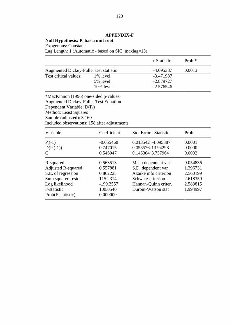
123

APPENDIX-F

Null Hypothesis: Pt has a unit root

Exogenous: Constant

Lag Length: 1 (Automatic - based on SIC, maxlag=13)

t-Statistic Prob.*

Augmented Dickey-Fuller test statistic -4.095387 0.0013

Test critical values: 1% level -3.471987

5% level -2.879727

10% level -2.576546

*MacKinnon (1996) one-sided p-values.

Augmented Dickey-Fuller Test Equation

Dependent Variable: D(Pt)

Method: Least Squares

Sample (adjusted): 3 160

Included observations: 158 after adjustments

Variable Coefficient Std. Error t-Statistic Prob.

Pt(-1) -0.055460 0.013542 -4.095387 0.0001

D(Pt(-1)) 0.747015 0.053576 13.94298 0.0000

C 0.546047 0.145304 3.757964 0.0002

R-squared 0.563513 Mean dependent var 0.054836

Adjusted R-squared 0.557881 S.D. dependent var 1.296731

S.E. of regression 0.862223 Akaike info criterion 2.560199

Sum squared resid 115.2314 Schwarz criterion 2.618350

Log likelihood -199.2557 Hannan-Quinn criter. 2.583815

F-statistic 100.0540 Durbin-Watson stat 1.994997

Prob(F-statistic) 0.000000

124

APPENDIX-G

Null Hypothesis: Mot has a unit root

Exogenous: Constant

Lag Length: 9 (Automatic - based on SIC, maxlag=13)

t-Statistic Prob.*

Augmented Dickey-Fuller test statistic -2.906593 0.0485

Test critical values: 1% level -3.474265

5% level -2.880722

10% level -2.577077

*MacKinnon (1996) one-sided p-values.

Augmented Dickey-Fuller Test Equation

Dependent Variable: D(Mot)

Method: Least Squares

Sample (adjusted): 11 160

Included observations: 150 after adjustments

Variable Coefficient Std. Error t-Statistic Prob.

Mot(-1) -0.011109 0.003822 -2.906593 0.0269

D(Mot(-1)) -0.912606 0.071900 -12.69270 0.0000

D(Mot(-2)) -0.005770 0.078935 -0.073103 0.9418

D(Mot(-3)) -0.005307 0.078974 -0.067199 0.9465

D(Mot(-4)) -0.756286 0.084035 -8.999667 0.0000

D(Mot(-5)) 0.681655 0.095413 7.144241 0.0000

D(Mot(-6)) -0.012471 0.081663 -0.152716 0.8788

D(Mot(-7)) 0.006098 0.081699 0.074635 0.9406

D(Mot(-8)) -0.873828 0.089158 -9.800891 0.0000

D(Mot(-9)) 0.778338 0.088867 8.758464 0.0000

C 384.5611 486.5393 0.790401 0.4306

R-squared 0.941166 Mean dependent var 13050.09

Adjusted R-squared 0.936934 S.D. dependent var 18131.67

S.E. of regression 4553.401 Akaike info criterion 19.75564

Sum squared resid 2.88E+09 Schwarz criterion 19.97642

Log likelihood -1470.673 Hannan-Quinn criter. 19.84534

F-statistic 222.3599 Durbin-Watson stat 1.914077

Prob(F-statistic) 0.000000

125

APPENDIX-H

Null Hypothesis: Ct has a unit root

Exogenous: Constant

Lag Length: 1 (Automatic - based on SIC, maxlag=13)

t-Statistic Prob.*

Augmented Dickey-Fuller test statistic -3.102681 0.0528

Test critical values: 1% level -3.471987

5% level -2.879727

10% level -2.576546

*MacKinnon (1996) one-sided p-values.

Augmented Dickey-Fuller Test Equation

Dependent Variable: D(Ct)

Method: Least Squares

Sample (adjusted): 3 160

Included observations: 158 after adjustments

Variable Coefficient Std. Error t-Statistic Prob.

Ct(-1) -0.037834 0.012194 -3.102681 0.0435

D(Ct(-1)) 0.388784 0.074028 5.251866 0.0000

C 1.619514 1.077278 1.503339 0.1348

R-squared 0.156520 Mean dependent var 0.001639

Adjusted R-squared 0.145636 S.D. dependent var 0.654588

S.E. of regression 0.605047 Akaike info criterion 1.851784

Sum squared resid 56.74271 Schwarz criterion 1.909934

Log likelihood -143.2909 Hannan-Quinn criter. 1.875400

F-statistic 14.38124 Durbin-Watson stat 2.059015

Prob(F-statistic) 0.000002

126

APPENDIX-I

Null Hypothesis: M2t has a unit root

Exogenous: Constant

Lag Length: 2 (Automatic - based on SIC, maxlag=13)

t-Statistic Prob.*

Augmented Dickey-Fuller test statistic -2.891236 1.0000

Test critical values: 1% level -3.472259

5% level -2.879846

10% level -2.576610

*MacKinnon (1996) one-sided p-values.

Augmented Dickey-Fuller Test Equation

Dependent Variable: D(M2t)

Method: Least Squares

Sample (adjusted): 4 160

Included observations: 157 after adjustments

Variable Coefficient Std. Error t-Statistic Prob.

M2t(-1) 0.008304 0.002872 -2.891236 0.0000

D(M2t(-1)) 0.301715 0.077500 3.893119 0.0001

D(M2t(-2)) 0.358129 0.078846 4.542144 0.0000

C 380.3171 1554.040 0.244728 0.8070

R-squared 0.929683 Mean dependent var 42542.47

Adjusted R-squared 0.928305 S.D. dependent var 57924.60

S.E. of regression 15509.88 Akaike info criterion 22.16149

Sum squared resid 3.68E+10 Schwarz criterion 22.23936

Log likelihood -1735.677 Hannan-Quinn criter. 22.19311

F-statistic 674.2918 Durbin-Watson stat 1.993049

Prob(F-statistic) 0.000000