The Munich Re Programme: Evaluating the Economics of Climate Risks and Opportunities in the Insurance Sector 

An evaluation of decadal probability forecasts from state-of-the-art climate models

Emma B. Suckling and Leonard A. Smith

21st October 2013

Centre for Climate Change Economics and Policy Working Paper No. 167

Munich Re Programme Technical Paper No. 19

Grantham Research Institute on Climate Change and the Environment

Working Paper No. 150

The Centre for Climate Change Economics and Policy (CCCEP) was established by the University of Leeds and the London School of Economics and Political Science in 2008 to advance public and private action on climate change through innovative, rigorous research. The Centre is funded by the UK Economic and Social Research Council and has five inter-linked research programmes:

1. Developing climate science and economics 2. Climate change governance for a new global deal 3. Adaptation to climate change and human development 4. Governments, markets and climate change mitigation 5. The Munich Re Programme - Evaluating the economics of climate risks and

opportunities in the insurance sector (funded by Munich Re) More information about the Centre for Climate Change Economics and Policy can be found at: http://www.cccep.ac.uk. The Munich Re Programme is evaluating the economics of climate risks and opportunities in the insurance sector. It is a comprehensive research programme that focuses on the assessment of the risks from climate change and on the appropriate responses, to inform decision-making in the private and public sectors. The programme is exploring, from a risk management perspective, the implications of climate change across the world, in terms of both physical impacts and regulatory responses. The programme draws on both science and economics, particularly in interpreting and applying climate and impact information in decision-making for both the short and long term. The programme is also identifying and developing approaches that enable the financial services industries to support effectively climate change adaptation and mitigation, through for example, providing catastrophe insurance against extreme weather events and innovative financial products for carbon markets. This programme is funded by Munich Re and benefits from research collaborations across the industry and public sectors. The Grantham Research Institute on Climate Change and the Environment was established by the London School of Economics and Political Science in 2008 to bring together international expertise on economics, finance, geography, the environment, international development and political economy to create a world-leading centre for policy-relevant research and training in climate change and the environment. The Institute is funded by the Grantham Foundation for the Protection of the Environment and the Global Green Growth Institute, and has five research programmes:

1. Global response strategies 2. Green growth 3. Practical aspects of climate policy 4. Adaptation and development 5. Resource security

More information about the Grantham Research Institute on Climate Change and the Environment can be found at: http://www.lse.ac.uk/grantham. This working paper is intended to stimulate discussion within the research community and among users of research, and its content may have been submitted for publication in academic journals. It has been reviewed by at least one internal referee before publication. The views expressed in this paper represent those of the author(s) and do not necessarily represent those of the host institutions or funders.

DRAFT

An evaluation of decadal probability forecasts1

from state-of-the-art climate models2

Emma B. Suckling and Leonard A. Smith

Centre for the Analysis of Time Series,

London School of Economics, Houghton Street,

London, WC2A 2AE, UK

Tel: +44 207 955 6015, Email: cats@lse.ac.uk

3

21st October 20134

ABSTRACT5

While state-of-the-art models of the Earth’s climate system have improved tremendously6

over the last twenty years, nontrivial structural flaws still hinder their ability to forecast the7

decadal dynamics of the Earth system realistically. Contrasting the skill of these models not8

only with each other but also with empirical models can reveal the space and time scales9

on which simulation models exploit their physical basis e!ectively and quantify their ability10

to add information to operational forecasts. The skill of decadal probabilistic hindcasts for11

annual global-mean and regional-mean temperatures from the EU ENSEMBLES project is12

contrasted with several empirical models. Both the ENSEMBLES models and a “Dynamic13

Climatology” empirical model show probabilistic skill above that of a static climatology for14

global-mean temperature. The Dynamic Climatology model, however, often outperforms the15

1

DRAFT

ENSEMBLES models. The fact that empirical models display skill similar to that of today’s16

state-of-the-art simulation models suggests that empirical forecasts can improve decadal17

forecasts for climate services, just as in weather, medium range, and seasonal forecasting. It18

is suggested that the direct comparison of simulation models with empirical models becomes19

a regular component of large model forecast evaluations. Doing so would clarify the extent20

to which state-of-the-art simulation models provide information beyond that available from21

simpler empirical models and clarify current limitations in using simulation forecasting for22

decision-support. Ultimately the skill of simulation models based on physical principles is23

expected to surpass that of empirical models in a changing climate; their direct comparison24

provides information on progress toward that goal which is not available in model-model25

intercomparisons.26

1. Introduction27

State-of-the-art dynamical simulation models of the Earth’s climate system1 are often28

used to make probabilistic predictions about the future climate and related phenomena with29

the aim of providing useful information for decision support (Anderson et al. 1999; UK-30

MetO"ce 2011; Weigela and Bowlerb 2009; Alessandri et al. 2011; Hagedorn et al. 2005;31

Hagedorn and Smith 2009; Meehl et al. 2009; Doblas-Reyes et al. 2010, 2011; IPCC 2007;32

Reifen and Toumi 2009). Evaluating the performance of such predictions from a model,33

or set of models, is crucial not only in terms of making scientific progress, but also in34

determining how much information may be available to decision-makers via climate services.35

1Models that use physical principles to simulate the Earth’s climate are often called general circula-

tion models (GCMs), coupled atmosphere-ocean global climate models (AOGCMs) or Earth system models

(ESMs). Such models are referred to as simulation models throughout this paper. The key distinction is

their explicit use of physical principles to simulate the system of interest. Simulation models are to be

contrasted with models based almost solely on observations, which are hereafter referred to as ‘empirical

models’ following (van den Dool 2007)

2

DRAFT

It is desirable to establish a robust and transparent approach to forecast evaluation, for the36

purpose of examining the extent to which today’s best available models are adequate over37

the spatial and temporal scales of interest for the task at hand. A useful reality check is38

provided by comparing the simulation models not only with other simulation models, but39

also with empirical models which do not include direct physical simulation.40

Decadal prediction brings several challenges for the design of ensemble experiments and41

their evaluation (Meehl et al. 2009; van Oldenborgh et al. 2012; Doblas-Reyes et al. 2010;42

Fildes and Kourentzes 2011; Doblas-Reyes et al. 2011); the analysis of decadal prediction43

systems will form a significant focus of the IPCC’s fifth assessment report (AR5). Decadal44

forecasts are of particular interest both for information on the impacts over the next ten45

years, as well as from the perspective of climate model evaluation. Hindcast experiments46

over an archive of historical observations allow approaches from empirical forecasting to be47

used for model evaluation. Such approaches can aid in the evaluation of forecasts from48

simulation models (Fildes and Kourentzes 2011; van Oldenborgh et al. 2012) and potentially49

increase the practical value of such forecasts through blending forecasts from simulation50

models with forecasts from empirical models that do not include direct physical simulation51

(Brocker and Smith 2008).52

This paper contrasts the performance of decadal probability forecasts from simulation53

models with that of empirical models constructed from the record of available observations.54

Empirical models are unlikely to yield realistic forecasts for the future once climate change55

moves the Earth system away from the conditions observed in the past. A simulation model,56

which aims to capture the relevant physical processes and feedbacks, is expected to be at57

least competitive with the empirical model. If this is not the case in the recent past, then58

it is reasonable to demand evidence that those particular simulation models are likely to be59

more informative than empirical models in forecasting the near future.60

A set of decadal simulations from the ENSEMBLES experiment (Hewitt and Griggs 2004;61

Doblas-Reyes et al. 2010), a precursor to the Coupled Model Intercomparison Project Phase62

3

DRAFT

5 (CMIP5) decadal simulations (Taylor et al. 2009) is considered. The ENSEMBLES proba-63

bility hindcasts are contrasted with forecasts from empirical models of the static climatology,64

persistence and a “Dynamic Climatology” model developed for evaluating other dynamical65

systems (Smith 1997; Binter 2011). Ensemble members are transformed into probabilistic66

forecasts via kernel dressing (Brocker and Smith 2008) and their quality quantified accord-67

ing to several proper scoring rules (Brocker and Smith 2006). The ENSEMBLES models do68

not demonstrate significantly greater skill than that of an empirical Dynamic Climatology69

model either for global mean temperature or for the land-based Giorgi region2 temperatures70

(Giorgi 2002).71

It is suggested that the direct comparison of simulation models with empirical models72

become a regular component of large model forecast evaluations. The methodology is easily73

adapted to other climate forecasting experiments and can provide a useful guide to decision-74

makers about whether state-of-the-art forecasts from simulation models provide additional75

information to that available from easily constructed empirical models.76

An overview of the ENSEMBLES models used for decadal probabilistic forecasting is77

discussed in section 2. The appropriate choice of empirical model for probabilistic decadal78

predictions forms the basis of section 3, while section 4 contains details of the evaluation79

framework and the transformation of ensembles into probabilistic forecast distributions. The80

performance of the ENSEMBLES decadal hindcast simulations is presented in section 581

and compared to that of the empirical models. Section 6 then provides a summary of82

conclusions and a discussion of their implications. The Supplementary Material includes83

graphics for models not shown in the main text, comparisons with alternative empirical84

models, results for regional forecasts and the application of alternative (proper) skill scores.85

The basic conclusion is relatively robust: the empirical Dynamic Climatology (DC) model86

2Giorgi regions are a set of land-based regions, defined in terms of simple rectangular areas and chosen

based on a qualitative understanding of current climate zones and on judgements about the performance of

climate models within these zones.

4

DRAFT

often outperforms the simulation models in terms of probability forecasting of temperature.87

2. Decadal prediction systems88

Given the timescales required to obtain fresh out-of-sample observations for the evalua-89

tion of decadal forecast systems, forecast evaluation is typically performed in-sample using90

hindcasts. Hindcasts (or retrospective forecasts) are predictions made as if they had been91

launched on dates in the past, and allow some comparison of model simulations with ob-92

servations. Of course, simulation models have been designed after the study of this same93

historical data, so their ability to reproduce historical observations carries significantly less94

weight than success out-of-sample. Failure in-sample, however, can be instructive.95

In a changing climate, even out-of-sample skill is no guarantee of future performance,96

due to the nonlinear nature of the response to external forcing (Smith 2002; Reifen and97

Toumi 2009; IPCC 2007). Nevertheless, the fact that only simulation models based on98

the appropriate physical principles are expected to be able to generalize to new physical99

conditions provides no evidence that today’s state-of-the-art simulation models can do so.100

Contrasting probability forecasts from simulation models with those from empirical models101

is one guide to gauging the additional information derived from the physical basis of the102

simulation model-based forecasts. In practice, the most skillful probability forecast is often103

based on combining the information from both simulation models and empirical models104

(van den Dool 2007; Hoeting et al. 1999; Unger et al. 2009; Brocker and Smith 2008; UK-105

MetO"ce 2011).106

Decadal predictions aim to accurately represent both the intrinsic variability and forced107

response to changes in the Earth system (Meehl et al. 2009). Decadal simulation models108

now assimilate observations of the current state of the Earth system as initial conditions109

in the model (Pierce et al. 2004; Troccoli and Palmer 2007)3. At present it is not clear110

3In reality, of course, no such distinct entities exist given the nonlinearity of the Earth System. The

5

DRAFT

whether initialising the model with observations at each forecast launch improves the skill of111

decadal forecasts (Pohlmann et al. 2009; Hawkins et al. 2011; Smith et al. 2007; Keenlyide112

et al. 2008; Smith et al. 2010; van Oldenborgh et al. 2012; Kim et al. 2012). At a more113

basic level, the ability to provide useful decadal predictions using simulation models is yet114

to be firmly established. Probabilistic hindcasts, based on simulations from Stream 2 of115

the ENSEMBLES project (further details of which can be found in (Doblas-Reyes et al.116

2010) and in the Appendix), do not demonstrate significantly more skill than that of simple117

empirical models.118

Figure 1 illustrates the 2-year running mean of simulated global mean temperature from119

the four simulation models in the multi-model ensemble experiment of the ENSEMBLES120

project over the full set of decadal hindcasts. Observations from the HadCRUT3 dataset121

and ERA40 reanalysis are shown for comparison. HadCRUT3 is used as the outcome archive122

for both the model evaluation and construction of the empirical model. Using ERA40 for123

the verification instead of HadCRUT3 does not change the conclusions about the model skill124

significantly (results not presented here). Global mean temperature is chosen for the analysis125

as simulation models are expected to perform better over larger spatial scales (IPCC 2007).126

Even at the global scale the raw simulation output is seen to di!er from the observations both127

in terms of absolute values, as well as in dynamics. Three of the four models display a sub-128

stantial model drift away from the observed global mean temperature, the ECHAM5 model129

is the exception. The fact that some of the models exhibit a substantial drift, but not oth-130

ers, reflects the fact that di!erent models employ di!erent initialisation schemes (Keenlyide131

et al. 2005). ECHAM5 both assimilates anomalies and forecasts anomalies. Assimilating132

anomalies is intended to reduce model drift4 (Pierce et al. 2004); the remaining models are133

initialised from observed conditions.134

nature of “intrinsic variability” is inextricably linked to the state of the Earth System; there is no separation

into a natural component and a forced component.4For point forecasts, forecasting anomalies allows an immediate apparent bias reduction at short lead

times on the order of the model’s systematic error.

6

DRAFT

A standard practice for dealing with model drift is to apply an empirical (linear) “bias135

correction” to the simulation runs (Stockdale 1997; Jolli!e and Stephenson 2003). Such a136

procedure both assumes that the bias of a given model at a given lead time does not change137

in the future, and is expected to break the connection between the underlying physical138

processes in the model and its forecast. Bias correction is often applied using the (sample)139

mean forecast error at each forecast lead time. The mean forecast error is shown as a function140

of lead time for global mean temperature in figure 2 for each of the ENSEMBLES models.141

Here, lead time 1 indicates the average of the first 12 months of each simulation, initialised142

in November of the launch year.143

The focus in this paper is on probability forecasts, specifically on contrasting the skill144

of simulation model probability forecasts with empirical model probability forecasts. On145

weather forecast timescales and in the medium range, simulation model based probability146

forecasts clearly have more skill than empirical model probability forecasts based on cli-147

matology (Hagedorn and Smith 2009). The question is whether, in the context of decadal148

probability forecasting, simulation models produce decadal probability predictions that are149

more skillful than simple empirical models. Answering this question requires defining an150

appropriate empirical model.151

3. Empirical models for decadal prediction152

Empirical models are common in forecast evaluation (Barnston et al. 1994; Colman and153

Davey 2003; van Oldenborgh et al. 2005, 2012; Lee et al. 2006; van den Dool 2007; Laepple154

et al. 2008; Krueger and von Storch 2011; Wilks 2011). They are used to quantify the155

information a simulation model adds beyond the naıve baseline the empirical models define.156

They have also been used to estimate forecast uncertainty (Smith 1992), both as benchmarks157

for simulation forecasts, and as a source of information to be combined with simulation model158

forecasts (van den Dool 2007; Unger et al. 2009; Smith 1997; UK-MetO"ce 2011; Hagedorn159

7

DRAFT

and Smith 2009).160

Empirical models based on historical observations cannot be expected to capture previ-161

ously unobserved dynamics. Two empirical models typically used in forecast evaluation are162

the climatological distribution and the persistence model. In the analysis below, a static163

climatology defines a probabilistic distribution generated through the kernel dressing and164

cross-validation procedures applied to the observational record (Brocker and Smith 2008;165

Hoeting et al. 1999), as outlined in section 4. Persistence forecasts are defined according166

to a similar procedure, based on the last observation, persisted as a single ensemble mem-167

ber for each launch. These models are not expected to prove ideal in a changing climate,168

nevertheless information regarding the ability (or inability) of a simulation model to outper-169

form these simple empirical models is of value. Alternative empirical models for probability170

forecasts, more appropriate for a changing climate, define a Dynamic Climatology based on171

ensemble random analogue prediction (eRAP) (Smith 1997; Paparella et al. 1997). Empir-172

ical forecasts are also used as benchmarks for evaluating point forecasts of decadal climate173

predictions (Fildes and Kourentzes 2011; van Oldenborgh et al. 2012; Doblas-Reyes et al.174

2010).175

Analogue forecasting uses the current state (perhaps with other recent states (Smith176

1997)) to define analogues within the observational record (van den Dool 1994; Lorenz 1963;177

van den Dool 2007). A distribution based on images of each analogue state (the observation178

immediately following the analogue state) then defines the ensemble forecast. Analogues may179

be defined in a variety of ways, including near neighbours either in observation space or in a180

delay reconstruction (Smith 1994, 1997). The ensemble members may be formed using the181

complete set of available analogue states (Dynamic Climatology (Smith 1997; Binter 2011)),182

or by selecting from the nearest neighbours at random, with the probability of selecting a183

particular neighbour related to the distance (in the state space) between the prediction point184

and the neighbour (the random analogue prediction method (Paparella et al. 1997)).185

The dynamic climatologies constructed below provide l-step ahead forecast distributions186

8

DRAFT

based on the current state and di!erences defined in the observational record. There are two187

approaches to forming such a Dynamic Climatology: (i) direct and (ii) iterated (Smith 1992).188

The direct Dynamic Climatology (DC) approach used below considers the l-step di!erences in189

the observational record (for example a 1-step di!erence might be the temperature di!erence190

between the current state and its immediately preceding state). A distribution is formed for191

each value of l from the corresponding di!erences using all the observations after some start192

date, thus the size of the ensemble decreases linearly with lead time due to the finite size of193

the archive. For a forecast of a scalar quantity, such as the global mean temperature below,194

the DC ensemble at lead time l launched at time t consists of the set of Nl values:195

ei = St +l #i, i = 1, ..., Nl, (1)

196

where St is the initial condition at time t and l#i, i = 1, ..., Nl is the set of lth di!erences in197

the observational record. Figure 3 illustrates the DC model for global mean temperature,198

launched at five-year intervals, as in the ENSEMBLES hindcasts. A true out-of-sample199

forecast up to the year 2015, initialised to the observed global mean temperature in 2004,200

is also included. Each lead time 1 forecast is based on an ensemble of 48 members. In201

real-time forecasting Nl = N ! l, while for cross-validation purposes the ensembles in figure202

3 use N ! l!1, omitting the #j corresponding to the year being forecast. Thus at lead time203

9 each forecast is based on an ensemble of 40 members. The DC approach is shown below204

to outperfom the ENSEMBLES models when forecasting global mean temperature.205

4. Probability forecasts from ensembles206

No forecast is complete without an estimate of forecast skill (Tennekes et al. 1987).207

Probability forecasts allow a complete description of the skill from an ensemble prediction208

system; they may be formed in several ways. The IPCC AR4 (IPCC 2007), for example,209

9

DRAFT

defines a likely range subjectively, applying the ‘sixty-forty’ rule5 to the mean of the CMIP3210

model global mean temperatures in 2100. Insofar as the forecast-outcome archive is larger211

for decadal timescales, objective statistical approaches are more easily deployed.212

Decadal probability forecasts are formed by transforming the ensemble into a probability213

distribution function via kernel dressing (Brocker and Smith 2008). A number of methods214

for this transformation exist and a selection will impact the skill of the forecast. The kernel215

dressed forecast based on an ensemble with N members is (Brocker and Smith 2008):216

p(y : x, !) =1

N!

N!

i=1

K

"y ! (xi + µ)

!

#, (2)

where xi is the ith ensemble member, µ is the o!set of the kernel mean (this o!set may have217

a di!erent value than the traditional “bias” term6) and ! is the kernel width. In this paper,218

the kernel, K, is taken to be a Gaussian function,219

K(") =1$(2#)

exp

"!1

2"2#. (3)

The kernel parameters are fitted by minimising a chosen skill score (Jolli!e and Stephenson220

2003) while avoiding information contamination7.221

The forecasts below are evaluated using the Ignorance score (Good 1952), defined as222

S(p(y), Y ) = !log2(p(Y )), (4)

5In chapter 10.5.4.6 of the AR4 (IPCC 2007) the “likely” range of global temperatures in 2100 are

provided for each of several scenarios. Each range falls “within 40 to +60% of the multi-model AOGCM

mean warming simulated for each scenario.” (pg 810). Similar results are shown in figure 5 of the Summary

for Policy Makers.6Kernel dressing and blending aim to provide good probability forecasts; this goal need not coincide with

minimizing the point forecast error of the ensemble mean.7Information contamination occurs when critical information is used in a hindcast which would not have

been available for a forecast actually made on the same launch date. While such contamination can never be

eliminated completely if the historical data is known, principled use of cross-validation can reduce its likely

impact.

10

DRAFT

where p(Y ) is the probability assigned to the verification, Y . By convention the smaller the223

score the more skillful the forecast (Jolli!e and Stephenson 2003).224

To contrast the skill of probability forecasts from two forecast systems it is useful to225

consider the relative Ignorance. The mean relative Ignorance of model 1 relative to model 2226

is defined as227

Srel(p1(y), p2(y), Y ) =1

F

F!

i=1

!log2

%p1(Yi)

p2(Yi)

&

= S(p1(y), Y )! S(p2(y), Y ). (5)

If p2 is taken as a reference forecast, then Srel defines ‘zero skill’ in the sense that p2 will228

have Srel = 0.229

Appropriate reference forecasts will depend on the task at hand: they may include a230

static climatological distribution, a dynamic climatology, another simulation model or em-231

pirical model. The relative Ignorance quantifies (in terms of bits) the additional information232

provided by forecasts from one model, above that of the reference. A relative Ignorance233

score of Srel(p1(y), p2(y), Y ) = !1 means that the model forecast places, on average, twice234

(that is 21) the probability mass on the verification than the reference forecast. Similarly, a235

score of236

Srel(p1(y), p2(y), Y ) = !1/2 means "41% (that is 21/2) more probability mass on average.237

In section 5, the static climatology, a persistence forecast and the DC model are chosen238

as references to measure performance against the ENSEMBLES simulation models. The239

parameters used to construct each empirical model forecast are each estimated under true-240

cross-validation: the forecast target decade is omitted from consideration.241

The ENSEMBLES forecast-outcome archive contains at most nine forecast-outcome242

pairs. That is, there are only nine forecast launch dates, each with a maximum lead time of243

ten years. Outside of true out-of-sample evaluation it is di"cult not to overfit the forecast244

and dressing parameters used to generate probability forecasts; the details of cross-validation245

11

DRAFT

can have a large impact. Extending the typical leave-some-out fitting protocol (Hastie et al.246

2001; Brocker and Smith 2008) to include the kernel dressing procedure reduces the sample247

size of the forecast-outcome archive from eight to seven pairs. This ‘true leave-some-out’248

procedure (Smith et al. 2013) will necessarily increase the sampling uncertainty, reflected249

through bootstrap resampling. In the case of the ENSEMBLES forecasts, adopting a true250

leave-some-out procedure reduces the apparent significance of the results; failing to introduce251

such a procedure, however, risks both information contamination and the suggestion that252

there is more skill than is to be expected in the simulation models. The most appropriate253

path cannot be determined with confidence until additional data becomes available.254

5. Results255

The skill of each of the four ENSEMBLES decadal prediction models has been evaluated256

relative to Dynamic Climatology (DC). The HadGem2 forecast distributions are shown as fan257

charts in figure 4 as an example. These forecast distributions tend to capture the observed258

global mean temperature, although the verification falls outside the 5th-95th percentile of259

the distribution more often than the expected 10% of the time. The distributions from the260

other ENSEMBLES simulation models (illustrated in the supplementary material) produce261

similar results.262

A set of forecast distributions for the DC model is shown in figure 5. This model was263

launched every year between 1960 and 2000, although only every fifth launch is illustrated, in264

keeping with the ENSEMBLES forecast launch dates. The increased number of launches for265

the DC model, each with a larger ensemble, allows more accurate statistics on its performance266

over the same range of the available observational data. Forecasts from the DC model show267

a similar distribution across each forecast launch, unlike those of the ENSEMBLES models.268

The verification also falls outside the 5th-95th percentile of the DC distributions on several269

occasions, similar to the distributions produced for the simulation models.270

12

DRAFT

Figure 6 shows the performance of all four ENSEMBLES simulation models and the271

DC empirical model in terms of Ignorance as a function of lead time. To test whether one272

model is systematically better than another requires considering the relative performance273

directly. The Ignorance of each model is computed relative to the static climatology shown274

in figure 7. True leave-some-out cross-validation is applied throughout. When the relative275

Ignorance is less than zero the model has skill relative to the static climatology. If the276

bootstrap resampling intervals of a model overlap zero, the model may be less skillful than277

the static climatology. In fact none of the simulation models consistently outperform the278

DC empirical model, which has among the lowest Ignorance scores. Figure 6 shows that the279

DC model significantly outperforms the static climatology across all lead times, on average280

placing approximately twice the probability mass on the verification (Srel # !1.0). The DC281

model using only launch dates every fifth year (to introduce a sampling uncertainty compa-282

rable to those of the ENSEMBLES model forecasts) shows a similar result but with slightly283

larger bootstrap resampling intervals as expected. For each of the ENSEMBLES models284

variations in skill between forecasts (for a given lead time) prevent the establishment of sig-285

nificant skill relative to the static climatology, despite the fact that both the IFS/HOPE and286

ARPEGE4/OPA models consistently produce relative Ignorance scores below zero at most287

lead times. The HadGem2 and ARPEGE4/OPA models, however, indicate that significant288

skill relative to static climatology can be established for early lead times. It is no surprise289

that the DC model performs better than the static climatology, since an increase in skill is290

almost certain to come from initialising each forecast to the observed temperature value at291

the forecast launch.292

Figure 8 shows the performance of each of the models relative to forecasts of persistence.293

Once again the DC model consistently shows relative Ignorance scores below zero across294

most lead times, while the ARPEGE4/OPA model scores below zero for early lead times (up295

to a lead time of five years), suggesting that forecasts from these models are more skillful296

than a persistence forecast over this range. In both cases the resampling bars cross the zero297

13

DRAFT

relative skill axis, clouding the significance of the result.298

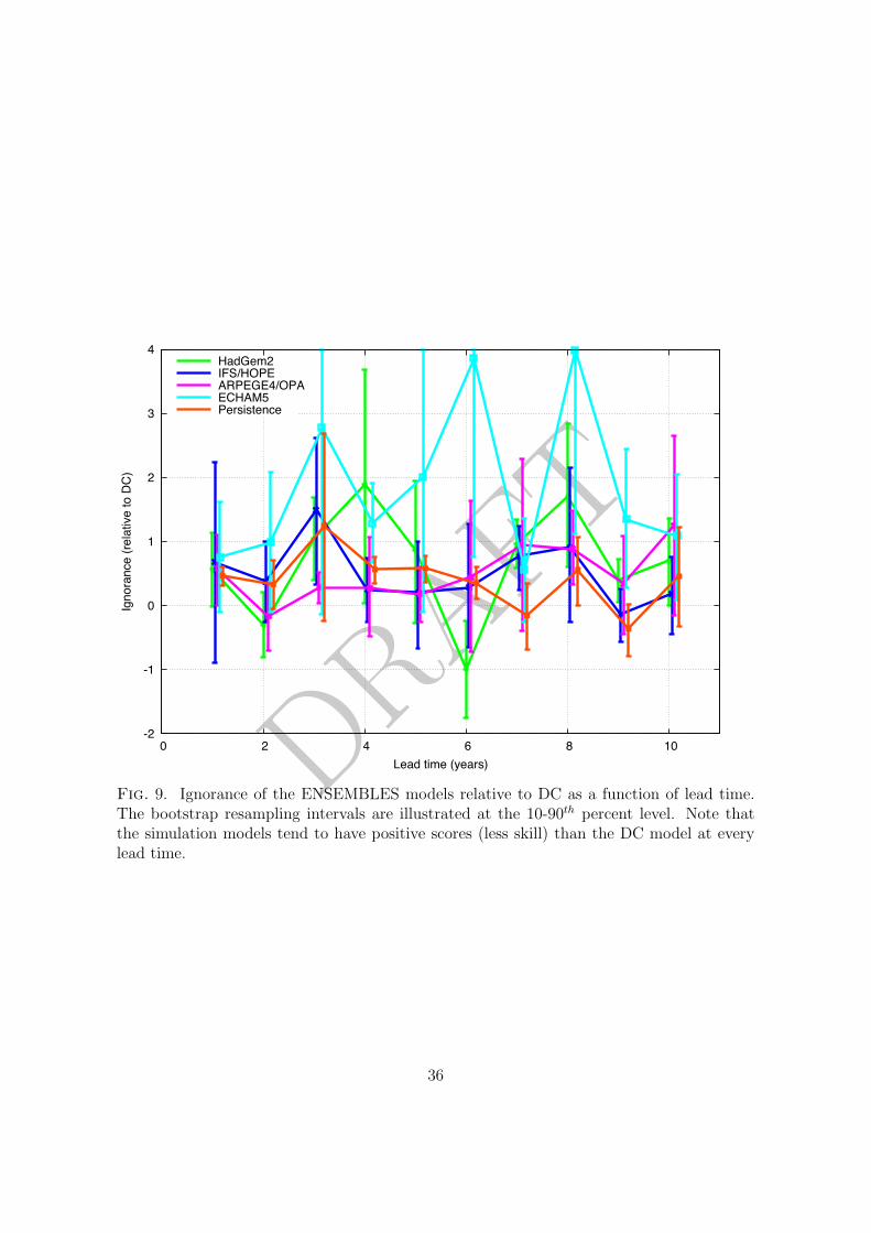
The skill of the ENSEMBLES simulation model forecasts is illustrated relative to the DC299

model in figure 9. None of the models in the ENSEMBLES multi-model ensemble demon-300

strates significant skill above the DC model at any lead time for global mean temperature.301

In fact all four simulation models show systematically less skill than the DC model. Similar302

results are found at smaller spatial scales (specifically the Giorgi regions (Giorgi 2002)),303

where the DC empirical model tends to outperform each of the ENSEMBLES simulation304

models (see the supplementary material).305

The ECHAM5 model generally has the least skill out of the ENSEMBLES models, par-306

ticularly for global mean temperature, with DC outperforming this model by several bits307

at lead times of up to ten years, although the bootstrap resampling intervals often overlap308

the zero line and also overlap with the intervals from the other simulation models in figure309

9. At global mean temperature scales the ARPEGE4/OPA model tends to perform better310

than the other ENSEMBLES models, perhaps surprisingly, since the raw simulation hind-311

casts from ARPEGE4/OPA contain a particularly large (but consistent) model drift relative312

to the other simulation models. Models requiring empirical drift corrections are less likely313

to produce realistic forecasts in a changing climate than they are in the current climate.314

Over the smaller spatial scales considered (the Giorgi regions) the ARPEGE4/OPA model315

no longer outperforms the other simulation models; no one ENSEMBLES model emerges as316

significantly better than any other (see Supplementary Material).317

The poor performance of the ECHAM5 simulation model might at first appear as a318

surprise, since the ensemble members from this model appear to be relatively close to the319

target values in figure 1. Note, however, that ECHAM5 initialises (and thus forecasts)320

model anomalies, not physical temperatures; the model forecasts then yield forecast model321

anomalies. In this case then, the systematic error of the model is partially accounted for322

when the model forecast anomalies are translated back into physical temperatures. The o!set323

applied within the kernel dressing procedure levels the playing field by accounting for the324

14

DRAFT

systematic errors in the other simulation models; the figures indicate that while ECHAM5325

may su!er less model drift due to this process (Keenlyide et al. 2005) it does not produce326

more skillful probability forecasts than the other ENSEMBLES simulation models.327

The ENSEMBLES experimental design also contains a perturbed physics ensemble from328

the UK Met O"ce Decadal Prediction System (DePreSys) (Doblas-Reyes et al. 2010), in329

which nine perturbed physics ensemble members are considered over the same set of hindcast330

launch dates. The DePreSys simulations contain only one initial condition ensemble member331

for each model version. In this case, the o!set and kernel parameters must be determined332

for each model version separately and the lack of any information on sensitivity to initial333

conditions limits the practical evaluation of the perturbed physics ensemble. The DePreSys334

hindcasts are therefore not considered for analysis here.335

While hindcast experiments can never provide true “out of sample” evaluation of a fore-336

casting system, it is possible to deny empirical models access to data observed after each337

launch date. In addition to the denial of what were e!ectively future observations, it is also338

necessary to illustrate that the skill of these Prelaunch empirical models8 does not depend339

sensitively on parameter tuning, as it is implausible that such tuning could have been done340

in real-time. The results reported below are robust to variations in the free parameters in341

the Prelaunch DC model (see Supplementary Material).342

Two Prelaunch empirical models were considered. The first is simply a direct climatology343

model where the observation archive is restricted to values prior to each launch date. The344

results are similar, in fact sometimes slightly better than, the standard DC model. Figure 10345

shows the skill of the Prelaunch DC model with a kernel width of (! = 0.08 and ! = 0.02)346

relative to the standard DC model, constructed under cross-validation; performance is robust347

8Arguably our “Prelaunch” model could be called a “simulated real-time” model. we resist this inasmuch

as the “future” was known when the experiment was designed, even though only the prelaunch observations

were used in constructing the model. “Prelauch” should be read to imply only that the data used was

restricted to that dated before the forecast launch date, it does not imply that (the impact of) all information

gleaned since that date was somehow forgotten.

15

DRAFT

to decreasing this width by more than an order of magnitude. A Prelaunch Trend model was348

also constructed to determine if the observed skill was due to a linear trend. The Prelaunch349

Trend model simply extends the linear fit to the observations from a fixed start-date (say,350

1950) to the launch date, and then uses the standard deviation of the residuals as the kernel351

width. The Prelaunch DC is more skillful than the Prelaunch Trend model, as shown in figure352

10. This result is robust to changing the start-date back towards 1900 (see Supplementary353

Material). It is important to stress that this trend model is not being advocated as a354

candidate empirical model, but only to address the specific question of whether the skill of355

the DC model comes only from the observed trend in global mean temperature. Much more356

e!ective methods for estimating statistical time-series models are available in this context357

(see for example (Fildes and Kourentzes 2011)).358

The results presented highlight several features for the experimental design of ensemble359

prediction systems and the impact that design has for the evaluation of probabilistic fore-360

casts. In hindcast experiment design, the number and type of ensemble members considered361

not only impact on the resolution of the prediction system, but also on the quality of the362

evaluation methodology: in the kernel dressing approach this impacts the accuracy of the363

estimated kernel o!set and spread parameters, as well as the cross-validation procedure.364

Sample size plays a major role and has consequences for the design of experiments and their365

evaluation. In particular the number of available forecasts and ensemble members can heav-366

ily influence the significance of the results, especially when the forecast-outcome archive is367

small. Large initial condition ensembles more clearly distinguish systematic model drift at368

a particular initial state from sensitivity to small changes in that initial state. Singleton369

ensembles, as in DePreSys, do not allow such a separation. With only a relatively short370

forecast-outcome archive and a small number of ensemble members per hindcast launch, the371

evaluation of the probabilistic forecasts su!ers from large sampling uncertainties. While it372

may not be possible to extend the duration of the observations, increasing the ensemble size373

can resolve some of the ambiguities involved in the cross-validation stage. In the case of374

16

DRAFT

DePreSys, it is suggested that future perturbed physics hindcast designs would benefit from375

including initial condition perturbations, as well as di!erent model versions. Further im-376

provements, in terms of increasing the statistical significance of the probabilistic evaluation,377

may be made by extending the size of the forecast-outcome archive further into the past, or378

where this is not possible, including intermediate launch dates to increase the sample size379

for the purpose of fitting the kernel dressing parameters.380

6. Conclusions381

The quality of decadal probability forecasts from the ENSEMBLES simulation models382

has been compared with that of reference forecasts from several empirical models. In general,383

the Stream 2 ENSEMBLES simulation models demonstrate less skill than the empirical DC384

model across the range of lead times from one to ten years. The result holds for a variety of385

proper scoring rules including Ignorance (Good 1952), the Proper Linear Score (PL) (Jolli!e386

and Stephenson 2003) and the continuous ranked probability score (CRPS) (Brocker and387

Smith 2006). A similar result holds on smaller spatial scales for the Giorgi Regions (see388

Supplementary Material). These new results for probability forecasts are consistent with389

evaluations of root-mean-square errors of decadal simulation models with other reference390

point forecasts (Fildes and Kourentzes 2011; van Oldenborgh et al. 2012; Weisheimer et al.391

2009). The DC probability forecasts often place up to 4 bits more information (or 24 times392

more probability mass) on the observed outcome than the ENSEMBLES simulation models.393

In the context of climate services, the comparable skill of simulation models and empirical394

models suggests that the empirical models will be of value for blending with simulation395

model ensembles; this is already done in ensemble forecasts for the medium range and on396

seasonal lead times. It also calls into question the extent to which current simulation models397

successfully capture the physics required for realistic simulation of the Earth System, and398

can thereby be expected to provide robust, reliable predictions (and, of course, to outperform399

17

DRAFT

empirical models) on longer time scales.400

The evaluation and comparison of decadal forecasts will always be hindered by the rela-401

tively small samples involved when contrasted with the case of weather forecasts; the decadal402

forecast-outcome archive currently considered is only half a century in duration. Advances403

both in modelling and in observation, as well as changes in the Earth’s climate, are likely to404

mean the relevant forecast-outcome archive will remain small. One improvement that could405

be made to clarify the skill of the simulation models is to improve the experimental design406

of hindcasts, in particular to increase the ensemble size used. For the ENSEMBLES models,407

each simulation ensemble consisted of only three members launched at five year intervals.408

Larger ensembles and more frequent forecast launch dates can ease the evaluation of skill409

without waiting for the forecast-outcome archive to grow larger9.410

The analysis of hindcasts can never be interpreted as an “out of sample” evaluation. The411

mathematical structure of simulation models, as well as parameterizations and parameter412

values, have been developed with knowledge of the historical data. Empirical models with a413

simple mathematical structure su!er less from this e!ect. Prelaunch empirical models based414

on the DC structure and using only observations before the forecast launch date also out-415

perform the ENSEMBLES simulation models. This result is robust over a range of ensemble416

interpretation parameters (that is, variations in the kernel width used). Both Prelaunch417

Trend models and persistence models are less skillful than the DC models considered.418

The comparison of near-term climate probability forecasts from Earth Simulation Models419

with those from Dynamic Climatology empirical models provides a useful benchmark as the420

simulation models improve in the future. The blending (Brocker and Smith 2008) of simu-421

lation models and empirical models is likely to provide more skillful probability forecasts in422

9As noted by a reviewer, it is possible that a DC model e!ectively captures all the available forecast

information given the uncertainty in the observations. This suggestion would be supported if the ENSEM-

BLES models were shown to be able to shadow (Smith 1997) over decades and, even with improved data

assimilation and using large ensembles, did not outperform empirical models; on the other hand it could be

easily falsified by a single simulation model which convincingly outperformed the empirical models.

18

DRAFT

Climate Services, both for policy and adaptation decisions. In addition, clear communica-423

tion of the (limited) expectations for skillful decadal forecasts can avoid casting doubt on424

well-founded physical understanding of the radiative response to increasing carbon dioxide425

concentration in the Earth’s atmosphere. Finally, these comparisons cast a sharp light on426

distinguishing whether current limitations in estimating the skill of a model arise from ex-427

ternal factors like the size of the forecast-outcome archive, or from the experimental design.428

Such insights are a valuable product of ENSEMBLES and will contribute to the experimental429

design of future ensemble decadal prediction systems.430

Acknowledgments431

This research was funded as part of the NERC EQUIP project (NE/H003479/1); it was432

also supported by the EU Framework 6 ENSEMBLES project (GOCE-CT-2003-505539-433

ENSEMBLES) and by both by the LSE’s Grantham Research Institute on Climate Change434

and the Environment and the ESRC Centre for Climate Change Economics and Policy,435

funded by the Economic and Social Research Council and Munich Re. L.A.S. gratefully436

acknowledges support of Pembroke College, Oxford. We also acknowledge the helpful com-437

ments and insights from Roman Binter, Hailiang Du, Ana Lopez, Falk Niehorster, David438

Stainforth and Erica Thompson, which helped shape this work, as well as discussions with439

H. van den Dool, G.-J. van Oldenborgh, A. Weisheimer and two anonymous reviewers which440

improved an earlier manuscript.441

Appendix: The Stream 2 ENSEMBLES decadal hind-442

cast experiments443

The set of decadal hindcast experiments from Stream 2 of the ENSEMBLES project444

simulations (Doblas-Reyes et al. 2010) have a similar experimental design to the seasonal445

19

DRAFT

hindcast experiments discussed in (Weisheimer et al. 2009). The decadal hindcasts consist446

of a set of initial condition ensembles, containing three ensemble members, initialised at447

launch, from four forecast systems - ARPEGE4/OPA (CERFACS), IFS/HOPE (ECMWF),448

HadGem2 (UKMO) and ECHAM5 (IFM-GEOMAR) - to produce a multi-model ensem-449

ble. A perturbed physics ensemble containing nine ensemble members from the DePreSys450

forecast system (based on the HadCM3 climate model) for both initialised and unassim-451

ilated simulations also forms part of the ENSEMBLES project. The hindcasts span the452

period 1960-2005, with simulations from each model launched at 5-year intervals, starting in453

November of the launch year and run over 10-year integrations. A full initialisation strategy454

was employed for the atmosphere and ocean using realistic estimates of their observed states455

(except for ECHAM5, which employed an anomaly initialisation scheme), with all the main456

radiative forcings prescribed and perturbations of the wind stress and SST fields made to457

sample initial condition uncertainty of the multi-model ensemble.458

459

REFERENCES460

Alessandri, A., A. Borrelli, A. Navarra, A. Arribas, M. Deque, P. Rogel, and A. Weisheimer,461

2011: Evaluation of probabilistic quality and value of the ensembles multimodel seasonal462

forecasts: Comparison with demeter. Monthly Weather Review, 139, 581–607.463

Anderson, J., H. van den Dool, A. Barnston, W. Chen, W. Stern, and J. Ploshay, 1999:464

Present-day capabilities of numerical and statistical models for atmospheric extratropi-465

cal seasonal simulation and prediction. Bulletin of the American Meteorological Society,466

80 (7).467

Barnston, A. G., et al., 1994: Long-lead seasonal forecasts - where do we stand? Bulletin of468

the American Meteorological Society, 75 (11), 2097–2114.469

20

DRAFT

Binter, R., 2011: Applied probabilistic forecasting. Ph.D. thesis, London School of Econmics470

and Political Science.471

Brocker, J. and L. A. Smith, 2006: Scoring probabilistic forecasts: The importance of being472

proper. Weather and Forecasting, 22, 382–388.473

Brocker, J. and L. A. Smith, 2008: From ensemble forecasts to predictive distributions.474

Tellus A, 60 (4), 663–678.475

Colman, A. and M. Davey, 2003: Statistical prediction of global sea-surface temperature476

anomalies. International Journal of Climatology, 23 (956), 1677–1697.477

Doblas-Reyes, F. J., M. A. Balmaseda, A. Weisheimer, and T. N. Palmer, 2011: Decadal478

climate prediction with the european centre for medium-range weather forecasts coupled479

forecast system: Impact of ocean observations. Journal of Geophysical Research - Atmo-480

spheres, 116 (D19111).481

Doblas-Reyes, F. J., A. Weisheimer, T. N. Palmer, J. M. Murphy, and D. Smith, 2010: Fore-482

cast quality assessment of the ensembles seasonal-to-decadal stream 2 hindcasts. Technical483

Memorandum ECMWF, 621.484

Fildes, R. and N. Kourentzes, 2011: Validation and forecasting accuracy in models of climate485

change. International Journal of Forecasting, 27 (4).486

Giorgi, F., 2002: Variability and trends of sub-continental scale surface climate in the twen-487

tieth century. part i: observations. Climate Dynamics, 18, 675–691.488

Good, I. J., 1952: Rational decsions. Journal of the Royal Statistical Society, XIV (1),489

107–114.490

Hagedorn, R., F. J. Doblas-Reyes, and T. N. Palmer, 2005: The rationale behind the success491

of multi-model ensembles in seasonal forecasting. part i: Basic concept. Tellus, A57, 219–492

233.493

21

DRAFT

Hagedorn, R. and L. A. Smith, 2009: Communicating the value of probabilistic forecasts494

with weather roulette. Meteorological Applications, 16 (2), 143–155.495

Hastie, T., R. Tibshirani, and J. Friedman, 2001: The elements of statistical learning.496

Springer, New York.497

Hawkins, E., J. Robson, R. Sutton, D. Smith, and N. Keenlyside, 2011: Evaluating the498

potential for statistical decadal predictions of sea surface temperature with a perfect model499

approach. Climate Dynamics, 1–15.500

Hewitt, C. D. and D. J. Griggs, 2004: Ensembles-based predictions of climate and their501

impacts. Eos, Transactions American Geophysical Union, 85 (52), 566.502

Hoeting, J. A., D. Madigan, A. E. Raftery, and C. T. Volinsky, 1999: Bayesian model503

averaging: A tutorial. Statistical Science, 14 (4).504

IPCC, 2007: Climate Change 2007: The Physical Science Basis. Contribution of Working505

Group I to the Fourth Assessment Report of the Intergovernmental Panel on Climate506

Change [S. Solomon and D. Qin and M. Manning and Z. Chen and M. Marquis and K.507

B. Averyt and M. Tignor and H. L. Miller (eds.)]. 996 pp, Cambridge University Press,508

Cambridge, United Kingdom and New York, NY USA.509

Jolli!e, I. T. and D. B. Stephenson, 2003: Forecast verification: A practitioner’s guide in510

atmospheric science. John Wiley and Sons Ltd.511

Keenlyide, N. S., M. Latif, M. Botzet, J. Jungclaus, and U. Schulzweida, 2005: A coupled512

method for initializing el nino southern oscillation forecasts using sea surface temperature.513

Tellus, 57A, 340–356.514

Keenlyide, N. S., M. Latif, J. Jungclaus, L. Kornblueh, and E. Roeckner, 2008: Advancing515

decadal-scale climate prediction in the north atlantic sector. Nature, 453 (06921), 84–88.516

22

DRAFT

Kim, H.-M., P. J. Webster, and J. A. Curry, 2012: Evaluation of short-term climate517

change prediction in multi-model cmip5 decadal hindcasts. Geophysical Research Letters,518

39 (L10701).519

Krueger, O. and J.-S. von Storch, 2011: A simple empirical model for decadal prediction.520

Journal of Climate, 24, 1276–1283.521

Laepple, T., S. Jewson, and K. Coughlin, 2008: Interannual temperature predictions using522

the cmip3 multi-model ensemble mean. Geophysical Research Letters, 35 (L10701).523

Lee, T. C. K., F. W. Zwiers, X. Zhang, and M. Tsao, 2006: Evidence of decadal climate pre-524

diction skill resulting from changes in anthropogenic forcing. Journal of Climate, 19 (20),525

5305–5318.526

Lorenz, E. N., 1963: Deterministic nonperiodic flow. Journal of Atmospheric Science, 20 (2),527

130–141.528

Meehl, G. A., et al., 2009: Decadal prediction: Can it be skillful? Bulletin of the American529

Meteorological Society, 90, 1467–1485.530

Paparella, F., A. Provenzale, L. A. Smith, C. Taricco, and R. Vio, 1997: Local random531

analogue prediction of nonlinear processes. Physics Letters A, 235 (3), 233–240.532

Pierce, D. W., T. P. Barnett, R. Tokmakian, A. Semtner, M. Maltrud, J. A. Lysne, and533

A. Craig, 2004: The acpi project, element 1: Initialising a coupled climate model from534

observed conditions. Climatic Change, 62 (1), 13–28.535

Pohlmann, H., J. H. Kohl, D. Stammer, and J. Marotzke, 2009: Initializing decadal climate536

predictions with gecco oceanic synthesis: E!ects on the north atlantic. Journal of Climate,537

22, 3926–3938.538

Reifen, C. and R. Toumi, 2009: Climate projections: Past performance no guarantee of539

future skill? Geophysical Research Letters, 36 (L13704).540

23

DRAFT

Smith, D. M., S. Cusack, A. W. Colman, C. K. Folland, G. R. Harris, and J. M. Murphy,541

2007: Improved surface temperature prediction for the coming decade from a global climate542

model. Science, 317, 796–799.543

Smith, D. M., R. Eade, N. J. Dunstone, D. Fereday, J. M. Murphy, H. Pohlmann, and544

A. A. Scaife, 2010: Skilful multi-year predictions of atlantic hurricane frequency. Nature545

Geoscience, 3 (1004), 846–849.546

Smith, L. A., 1992: Identification and prediction of low-dimensional dynamics. Physica D,547

58 (1-4), 50–76.548

Smith, L. A., 1994: Local optimal prediction: Exploiting strangeness and the variation of sen-549

sitivity to initial condition. Philosophical Transactions of the Royal Society A, 348 (1688),550

371–381.551

Smith, L. A., 1997: The maintenance of uncertainty. Proc. International School of Physics552

“Enrico Fermi”, Course CXXXIII, 177–246, Societ’a Italiana di Fisica, Italy.553

Smith, L. A., 2002: What might we learn from climate forecasts? Proceedings of the National554

Academy of Science, 4 (99), 2487–2492.555

Smith, L. A., H. Du, F. Niehorster, and E. B. Suckling, 2013: An evaluation of probabilistic556

skill from ensemble seasonal forecasts. submitted to the Quarterly Journal of the Royal557

Meteorological Society.558

Stockdale, T. N., 1997: Coupled ocean-atmosphere forecasts in the presence of climate drift.559

Monthly Weather Review, 125, 809–818.560

Taylor, K. E., R. J. Stou!er, and G. A. Meehl, 2009: A summary of the cmip5 experimental561

design. http: // cmip-pcmdi. llnl. gov/ cmip5/ docs/ Taylor_ CMIP5_ design. pdf .562

Tennekes, H., A. P. M. Baede, and J. D. Opsteegh, 1987: Forecasting forecast skill. Proceed-563

ings ECMWF Workshop on Predictability, ECMWF, Reading, UK, 277–302.564

24

DRAFT

Troccoli, A. and T. N. Palmer, 2007: Ensemble decadal predictions from analysed initial565

conditions. Philosophical Transactions of the Royal Society A, 365, 2179–2191.566

UK-MetO"ce, 2011: 3-month outlook for uk contingency planning. http: // www.567

metoffice. gov. uk/ media/ pdf/ g/ o/ 3-month_ Outlook_ user_ guidance-150. pdf .568

Unger, D., H. van den Dool, E. O’Lenic, and D. Collins, 2009: Ensemble regression. Monthly569

Weather Review, 137 (2365-2379).570

van den Dool, H. M., 1994: Long-range weather forecasts through numerical and empirical571

methods. Dynamics of Atmospheres and Oceans, 20 (3), 247–270.572

van den Dool, H. M., 2007: Empirical methods in short-term climate prediction. Oxford573

University Press.574

van Oldenborgh, G. J., M. Balmaseda, L. Ferranti, T. Stockdale, and D. Anderson, 2005:575

Evaluation of atmospheric fields from the ecmwf seasonal forecasts over a 15-year period.576

Journal of Climate, 18, 3250–3269.577

van Oldenborgh, G. J., F. J. Doblas-Reyes, B. Wouters, and W. Hazeleger, 2012: Decadal578

prediction skill in a multi-model ensemble. Climate Dynamics, 38 (7-8), 1263–1280.579

Weigela, A. P. and N. E. Bowlerb, 2009: Can multi-model combination really enhance predic-580

tion skill of probabilistic ensemble forecasts? Quarterly Journal of the Royal Meteorological581

Society, 135, 535–539.582

Weisheimer, A., et al., 2009: Ensembles - a new multi-model ensemble for seasonal-to-583

annual predictions: Skill and progress beyond demeter in forecasting tropical pacific ssts.584

Geophysical Research Letters, 36 (L21711).585

Wilks, D. S., 2011: Statistical Methods in the Atmospheric Sciences, 3rd Edition, Vol. 100.586

Academic Press.587

25

DRAFT

List of Figures588

1 Global mean temperature (2 year running mean) for the four forecast systems589

- HadGem2 (UKMO), IFS/HOPE (ECMWF), ARPEGE4/OPA (CERFACS)590

and ECHAM5 (IFM-GEOMAR) - that form Stream 2 of the ENSEMBLES591

decadal hindcast simulations (Doblas-Reyes et al. 2010). HadCRUT3 obser-592

vations and ERA40 reanalysis are also shown for comparison. Note that the593

scale on the vertical axis for the ARPEGE4/OPA model is di!erent to the594

other three panels, reflecting the larger bias in this model. 28595

2 Mean forecast error as a function of lead time across the set of decadal hind-596

casts for each of the ENSEMBLES simulation models as labelled. Note that597

the scale on the vertical axis for the ARPEGE4/OPA model is di!erent to598

the other three panels, reflecting the larger bias in this model. 29599

3 Dynamic climatology (DC) over the period of the ENSEMBLES hindcasts600

(figure 1). HadCRUT3 (from which the DC model is constructed) is shown601

for comparison. 30602

4 Forecast distributions for HadGem2 (UKMO) for the 5-95th percentile. The603

HadCRUT3 observed temperatures are shown in blue. The forecasts are ten604

years long and lauched every five years, and so the fan charts would overlap;605

to avoid this they are presented on two panels. The top (bottom) panel606

illustrates forecasts launched in ten year intervals from 1960 (1965). 31607

5 Forecast distribution for every fifth launch from the Dynamic Climatology608

(DC) model for the 5-95th percentile. The HadCRUT3 observed temperatures609

are shown in blue. The forecasts are ten years long and lauched every five610

years, and so the fan charts would overlap; to avoid this they are presented611

on two panels. The top (bottom) panel illustrates forecasts launched in ten612

year intervals from 1960 (1965). 32613

26

DRAFT

6 Ignorance as a function of lead time for each of the four ENSEMBLES hindcast614

simulation models and the DC model relative to the static climatology. The615

bootstrap resampling intervals are illustrated at the 10-90th percent level. The616

DC model is shown to be significantly more skillful than static climatology617

at all lead times, whereas the ARPEGE4/OPA and IFS/HOPE models are618

significantly more skillful than static climatology at early lead times. 33619

7 Probability density for the static climatology used in the paper with obser-620

vations over the period 1960-2010 (from HadCRUT3) illustrated as points on621

the x-axis for reference. 34622

8 Ignorance of the ENSEMBLES models and DC relative to persistence fore-623

casts as a function of lead time. The DC model has negative relative Ignorance624

scores up to 6 years ahead, indicating it is significantly more skillful than per-625

sistence forecasts at early lead times. The ENSEMBLES models tend to have626

positive scores, particularly at longer lead times, with bootstrap resampling627

intervals that overlap with the zero skill line. The bootstrap resampling in-628

tervals are illustrated at the 10-90th percent level. 35629

9 Ignorance of the ENSEMBLES models relative to DC as a function of lead630

time. The bootstrap resampling intervals are illustrated at the 10-90th percent631

level. Note that the simulation models tend to have positive scores (less skill)632

than the DC model at every lead time. 36633

10 Ignorance of the Prelaunch DC and Prelaunch Trend models relative to the634

standard DC model as a function of lead time. The HadGem2 model from635

ENSEMBLES is also shown. It is shown that the Prelaunch DC model is636

not significantly less skillful than the standard DC model and is robust to637

variations in parameter tuning. The Prelaunch linear trend model is, however,638

generally shown to be less skillful than the standard DC model. The bootstrap639

resampling intervals are illustrated at the 10-90th percent level. 37640

27

DRAFT 13

13.5

14

14.5

15

1960 1970 1980 1990 2000 2010

Tem

pera

ture

(˚ C

)

Year

HadGem2(UKMO) - 3 ensemble members

HadCRUT3ERA40

13

13.5

14

14.5

15

1960 1970 1980 1990 2000 2010

Tem

pera

ture

(˚ C

)

Year

IFS/HOPE(ECMWF) - 3 ensemble members

HadCRUT3ERA40

9

10

11

12

13

14

15

1960 1970 1980 1990 2000 2010

Tem

pera

ture

(˚ C

)

Year

ARPEGE/OPA(CERFACS) - 3 ensemble members

HadCRUT3ERA40

13

13.5

14

14.5

15

1960 1970 1980 1990 2000 2010

Tem

pera

ture

(˚ C

)

Year

ECHAM5/OM1(IFM-GEOMAR) - 3 ensemble members

HadCRUT3ERA40

Fig. 1. Global mean temperature (2 year running mean) for the four forecast systems -HadGem2 (UKMO), IFS/HOPE (ECMWF), ARPEGE4/OPA (CERFACS) and ECHAM5(IFM-GEOMAR) - that form Stream 2 of the ENSEMBLES decadal hindcast simulations(Doblas-Reyes et al. 2010). HadCRUT3 observations and ERA40 reanalysis are also shownfor comparison. Note that the scale on the vertical axis for the ARPEGE4/OPA model isdi!erent to the other three panels, reflecting the larger bias in this model.

28

DRAFT-0.4

-0.2

0

0.2

0.4

0 2 4 6 8 10

Mea

n Er

ror (

T(O

bs)-T

(Mod

el))

Lead Time (Years)

HadGem2

-0.4

-0.2

0

0.2

0.4

0 2 4 6 8 10

Mea

n Er

ror (

T(O

bs)-T

(Mod

el))

Lead Time (Years)

IFS/HOPE

3

3.5

4

4.5

5

0 2 4 6 8 10

Mea

n Er

ror (

T(O

bs)-T

(Mod

el))

Lead Time (Years)

ARPEGE4/OPA

-0.4

-0.2

0

0.2

0.4

0 2 4 6 8 10

Mea

n Er

ror (

T(O

bs)-T

(Mod

el))

Lead Time (Years)

ECHAM5/OM1

Fig. 2. Mean forecast error as a function of lead time across the set of decadal hindcastsfor each of the ENSEMBLES simulation models as labelled. Note that the scale on thevertical axis for the ARPEGE4/OPA model is di!erent to the other three panels, reflectingthe larger bias in this model.

29

DRAFT

13

13.5

14

14.5

15

15.5

1960 1970 1980 1990 2000 2010 2020

Tem

pera

ture

(˚C

)

Year

Dynamic Climatology (DC)

HadCRUT3

Fig. 3. Dynamic climatology (DC) over the period of the ENSEMBLES hindcasts (figure1). HadCRUT3 (from which the DC model is constructed) is shown for comparison.

30

DRAFT

13

13.

5

14

14.

5

15

15.

5

Temperature (˚C)

Had

Gem

2

13

13.

5

14

14.

5

15

15.

5 196

0 1

970

198

0 1

990

200

0 2

010

Year

0.05

-0.9

50.

1-0.

90.

15-0

.85

0.2-

0.8

0.25

-0.7

50.

3-0.

7

0.35

-0.6

50.

4-0.

60.

45-0

.55

Fig. 4. Forecast distributions for HadGem2 (UKMO) for the 5-95th percentile. The Had-CRUT3 observed temperatures are shown in blue. The forecasts are ten years long andlauched every five years, and so the fan charts would overlap; to avoid this they are pre-sented on two panels. The top (bottom) panel illustrates forecasts launched in ten yearintervals from 1960 (1965).

31

DRAFT

13

13.

5

14

14.

5

15

15.

5

Temperature (˚C)

Dyn

amic

Clim

atol

ogy

(DC

)

13

13.

5

14

14.

5

15

15.

5 196

0 1

970

198

0 1

990

200

0 2

010

Year

0.05

-0.9

50.

1-0.

90.

15-0

.85

0.2-

0.8

0.25

-0.7

50.

3-0.

7

0.35

-0.6

50.

4-0.

60.

45-0

.55

Fig. 5. Forecast distribution for every fifth launch from the Dynamic Climatology (DC)model for the 5-95th percentile. The HadCRUT3 observed temperatures are shown in blue.The forecasts are ten years long and lauched every five years, and so the fan charts wouldoverlap; to avoid this they are presented on two panels. The top (bottom) panel illustratesforecasts launched in ten year intervals from 1960 (1965).

32

DRAFT

-2

-1

0

1

2

3

4

0 2 4 6 8 10

Igno

ranc

e (re

lativ

e to

sta

tic c

limat

olog

y)

Lead time (years)

HadGem2IFS/HOPEARPEGE4/OPAECHAM5DCDC (fifth year launch)

Fig. 6. Ignorance as a function of lead time for each of the four ENSEMBLES hindcast simu-lation models and the DC model relative to the static climatology. The bootstrap resamplingintervals are illustrated at the 10-90th percent level. The DC model is shown to be signifi-cantly more skillful than static climatology at all lead times, whereas the ARPEGE4/OPAand IFS/HOPE models are significantly more skillful than static climatology at early leadtimes.

33

DRAFT

0

0.002

0.004

0.006

0.008

0.01

0.012

13.6 13.8 14 14.2 14.4 14.6 14.8

Den

sity

Global mean temperature (˚C)

Static ClimatologyHadCRUT3

Fig. 7. Probability density for the static climatology used in the paper with observationsover the period 1960-2010 (from HadCRUT3) illustrated as points on the x-axis for reference.

34

DRAFT

-2

-1

0

1

2

3

0 2 4 6 8 10

Igno

ranc

e (re

lativ

e to

per

siste

nce)

Lead time (years)

HadGem2IFS/HOPEARPEGE4/OPAECHAM5DC

Fig. 8. Ignorance of the ENSEMBLES models and DC relative to persistence forecastsas a function of lead time. The DC model has negative relative Ignorance scores up to 6years ahead, indicating it is significantly more skillful than persistence forecasts at earlylead times. The ENSEMBLES models tend to have positive scores, particularly at longerlead times, with bootstrap resampling intervals that overlap with the zero skill line. Thebootstrap resampling intervals are illustrated at the 10-90th percent level.

35

DRAFT

-2

-1

0

1

2

3

4

0 2 4 6 8 10

Igno

ranc

e (re

lativ

e to

DC)

Lead time (years)

HadGem2IFS/HOPEARPEGE4/OPAECHAM5Persistence

Fig. 9. Ignorance of the ENSEMBLES models relative to DC as a function of lead time.The bootstrap resampling intervals are illustrated at the 10-90th percent level. Note thatthe simulation models tend to have positive scores (less skill) than the DC model at everylead time.

36

DRAFT

-2

-1

0

1

2

3

4

0 2 4 6 8 10

Igno

ranc

e (re

lativ

e to

cro

ss-v

alid

atio

n D

C)

Lead time (years)

HadGem2Prelaunch DC (!=0.08)Prelaunch DC (!=0.02)Prelaunch linear trend

Fig. 10. Ignorance of the Prelaunch DC and Prelaunch Trend models relative to the standardDC model as a function of lead time. The HadGem2 model from ENSEMBLES is also shown.It is shown that the Prelaunch DC model is not significantly less skillful than the standardDC model and is robust to variations in parameter tuning. The Prelaunch linear trend modelis, however, generally shown to be less skillful than the standard DC model. The bootstrapresampling intervals are illustrated at the 10-90th percent level.

37

DRAFT

An evaluation of decadal probability forecasts from1

state-of-the-art climate models - Supplementary2

Material3

Emma B. Suckling and Leonard A. Smith4

October 21, 20135

1. Introduction6

The following material is a supplement to ‘An evaluation of decadal probability forecasts7

from state-of-the-art climate models’, in which the perfomance of simulation models from8

Stream 2 of the ENSEMBLES decadal hindcasts (Doblas-Reyes et al. 2010) are contrasted9

with the empirical dynamic climatology (DC) model over global and Giorgi region scales.10

Further details about transforming ensemble simulations into probabilistic distributions are11

presented below in Section 2. In Section 3 it is shown that the DC empirical model outper-12

forms the ENSEMBLES simulation models by several bits at most lead times and for every13

region studied. In Section 4 the robustness of the results in the main manuscript are evalu-14

ated by using alternative proper scoring rules, namely the proper linear (PL) and continuous15

1

DRAFT

ranked probability scores (CRPS). It is shown that the results are robust to the scoring rule16

chosen. Finally, in Section 5 the performance of alternative empirical models are considered,17

namely a ‘Prelaunch linear trend’ approach and ‘Prelaunch DC model’. It is shown that the18

Prelaunch DC model performs to a similar quality as the standard DC approach employed19

in the main manuscript, and is robust to the kernel parameters and anchor year chosen20

to fit the model. Further details about generating the probabilistic DC forecasts and the21

robustness of the results to the model parameter choices are also provided in Section 5.22

2. Probabilistic forecast distributions for the ENSEM-23

BLES simulation models24

Figures 1, 2 and 3 illustrate the probabilistic forecast distributions for the ENSEMBLES25

simulation models, generated by kernel dressing the ensemble members as described in the26

main manuscript and below under cross-validation (the forecast distributions for HadGem227

are illustrated in figure 3 in the main manuscript).28

Information contamination is a significant concern in the evaluation of decadal forecasts.29

Given that the total duration of hindcast experiments is typically fifty years, there are30

very few independent decadal periods in the forecast-outcome archive. Cross-validation ap-31

proaches attempt to maximise the size of the forecast-outcome archive (to increase statistical32

significance) while avoiding the use of information from a given forecast target period being33

used in the evaluation of that forecast. It is crucial to also avoid information contamination34

by inadvertently using information from the target decade when interpreting the ensemble35

2

DRAFT

into a forecast distribution (Brocker and Smith 2008). This cannot be done rigorously in36

the case of simulation models, as the structure and parameters of the models themselves37

have evolved in light of the observations of the last fifty years. The true-leave-one-out cross-38

validation procedure described in the main maunuscript avoids any explict use of data from39

within the target forecast period, even as its implicit use cannot be avoided. In practice this40

is achieved by leaving out the target decade, then using a standard leave-one-out procedure41

to fit the kernel parameters for each forecast in turn.42

Figure 4 shows an example of the kernel parameters used for the HadGem2 model, fitted43

using the true-leave-one-out protocol. The top two panels of figure 4 illustrate the mean44

Ignorance score as a function of kernel width over the full set of hindcast simulations (i.e.45

with no cross-validation) for lead time one and lead time six. The vertical bars indicate46

the values of the kernel width parameter that were used for each forecast using the true-47

leave-one-out approach. In both cases the fact that fewer than nine vertical bars are visible48

indicates that several of the forecasts were generated using the same kernel width values.49

Note that at lead time six for HadGem2 the kernel width values used are much smaller than50

for lead time one (and for all other lead times). In this particular case the model is rewarded51

for a forecast distribution that has kernel widths much smaller than the standard deviation52

of the ensemble spread.53

The bottom panels of figure 4 show the mean Ignorance as a function of kernel o!set54

over the full set of hindcast simulations. Once again the vertical bars indicate the values of55

o!set that were used for the individual forecasts, based on minimising Ignorance through the56

true-leave-one out protocol. Once again, at lead time six the fitting protocol favours a kernel57

o!set under true-leave-one-out cross-validation that falls outside the minimum Ignorance58

3

DRAFT

value without cross-validation. The result for lead time one is typical of the kernel o!set59

values attained for the other lead times.60

3. Regional analysis61

Figures 5 to 25 show Ignorance as a function of lead time for each of the ENSEMBLES62

models relative to the DC empirical model for surface air temperature over each of the63

land-based Giorgi regions (Giorgi 2002). At Giorgi region scales the decadal probability64

forecasts from the ENSEMBLES models perform to a similar quality as for the global mean65

temperature in some cases, or significantly worse in others. In some regions and at some66

lead times DC outperforms the ENSEMBLES models by more than 4 bits; DC placing over67

16 (24) times more probability mass on the verification than the simulation model. In these68

figures no simulation model demonstrates skill significantly above the DC model for any69

lead time or any region; positive values of the relative Ignorance performance measure are70

reported in all of the cases below.71

4. Robustness to the peformance measure72

While Ignorance is e!ectively the only proper local score for the evaluation of probability73

forecasts (Good 1952), there are a variety of other proper scores that are commonly used74

in forecast evaluation (Jolli!e and Stephenson 2003). Figures 26 and 27 demonstrate that75

the results presented in the main text for global mean surface temperature are robust when76

considered under two alternative scores, the Proper Linear score (PL) and the Continuous77

4

DRAFT

Ranked Probability Score (CRPS) (Jolli!e and Stephenson 2003). In each of these cases,78

the lower the score the better the forecast. In each case all the models are ranked similarly79

by the di!erent scores, with DC demonstrating lower scores compared to the ENSEMBLES80

models.81

5. Alternative empirical models82

The use of hindcasts in forecast evaluation unavoidably introduces information contam-83

ination, as the target of the hindcast is known when the hindcast is made. Thus it is useful84

to demonstrate that the results of hindcast evaluation are robust to variations in the param-85

eters and even the structure of empirical models, as doing so can identify cases where the86

hindcast system may have been over-fit in-sample. For the DC empirical model presented in87

this paper, all data from each target decade being forecast was withheld when constructing88

that forecast to avoid information contamination. Further avoidance of such information89

contamination can be achieved in the case of empirical models by using only data from a90

period prior to each forecast launch date and by using a simple model structure. In this91

section, two Prelaunch empirical models (defined in the main text) are illustrated below,92

and their robustness to the model parameters examined.93

The Prelaunch Dynamic Climatology (Prelaunch DC) model is structurally identical to94

the DC model of the main manuscript, however only inputs dated before the launch date are95

used either in the ensemble forecast or in its interpretation into a probability distribution,96

and so on. While the kernel width used in the standard DC model is determined by cross-97

validation, this need not be done for the Prelaunch DC model as only the observations98

5

DRAFT

available before the forecast launch time are used.99

Examining the of the score to variations in the parameters can reveal overfitting. Figure100

28 shows the skill of the Prelaunch DC for values of the kernel width ranging from 0.02 to101

0.16 for forecast lead times of one to ten years. Ignorance relative to the standard DC model102

is shown. The sensitivity of the Prelaunch DC model to variation in the starting date for the103

forecast-outcome archive (not shown) is less than the sensitivity to the kernel width. Start104

dates from 1900 to 1950 were considered; the later start dates tend to yield more skilful105

models. The Prelaunch DC discussed in the main text uses a start date of 1950 and a width106

of 0.08, although this value does not correspond to the lowest in-sample skill - as shown in107

figure 29. Furthermore the ensemble interpretation of the simulations models reported in108

this paper use data both before and after the target window, giving those simulation models109

an unquantified advantage over the empirical models defined here.110

Figure 29 shows the mean Ignorance score over the set of DC and Prelaunch DC hindcasts111

as a function of the kernel width parameter. The panels on the left of figure 29 correspond112

to lead times one (a), six (c) and ten (e) respectively for the standard DC model, and the113

panels on the right correspond to the same lead times for the Prelaunch DC model. In114

each case the vertical bars correspond to the values of kernel spread adopted for each model115

in the main manuscript (note that for the standard DC model these values were attained116

under true-leave-one-out cross-validation and for the Prelaunch DC model a value of 0.08117

was chosen since cross-validation is not necessary in this case). The fact that there is no118

significant di!erence in skill between the standard DC and Prelaunch DC models over a119

range of kernel dressing parameters indicates that the overall conclusions drawn from the120

ENSEMBLES model evaluations are not overly sensitive to the particular choice of DC or121

6

DRAFT

Prelaunch DC model parameters.122

A Prelaunch trend model is also discussed in the main text. This model is fully defined123

by the initial time anchor from which the trend is estimated. Figure 30 shows the skill of124

this model relative to the standard DC model for several anchor times between 1900 and125

1950. The results in the main text use the 1950 anchor time. It is shown that although126

there is some sensitivity to the anchor time, all the Prelaunch trend models are generally127

less skillful than the standard DC model.128

The figures presented in this supplementary material demonstrate that the skill of the129

empirical models is robust under relatively large variations in their free parameters. This130

level of skill remains comparable with, and in some cases superior to, that of the simulation131

models from ENSEMBLES.132

133

REFERENCES134

Brocker, J. and L. A. Smith, 2008: From ensemble forecasts to predictive distributions.135

Tellus A, 60 (4), 663–678.136

Doblas-Reyes, F. J., A. Weisheimer, T. N. Palmer, J. M. Murphy, and D. Smith, 2010: Fore-137

cast quality assessment of the ensembles seasonal-to-decadal stream 2 hindcasts. Technical138

Memorandum ECMWF, 621.139

7

DRAFT

Giorgi, F., 2002: Variability and trends of sub-continental scale surface climate in the twen-140

tieth century. part i: observations. Climate Dynamics, 18, 675–691.141

Good, I. J., 1952: Rational decsions. Journal of the Royal Statistical Society, XIV (1),142

107–114.143

Jolli!e, I. T. and D. B. Stephenson, 2003: Forecast verification: A practitioner’s guide in144

atmospheric science. John Wiley and Sons Ltd.145

8

DRAFT

List of Figures146

1 Forecast distributions for IFS/HOPE (ECMWF) for the 5-95th percentile.147

The HadCRUT3 observed temperatures are shown in blue. Each forecast is148

ten years long and they are launched every five years. To avoid overlap of149

the fan charts they are presented on two panels. The top (bottom) panel150

illustrates forecasts launched in ten year intervals from 1960 (1965). It is151

shown that the observed global mean temperature often falls outside the 5-152

95th percentile of the predicted distributions. 16153

2 Forecast distributions for ARPEGE/OPA (CERFACS) for the 5-95th per-154

centile. The HadCRUT3 observed temperatures are shown in blue. The top155

(bottom) panel illustrates forecasts launched in ten year intervals from 1960156

(1965). It is shown that the observed global mean temperature often falls157

outside the 5-95th percentile of the predicted distributions. 17158

3 Forecast distributions for ECHAM5 (IFM-GEOMAR) for the 5-95th per-159

centile. The HadCRUT3 observed temperatures are shown in blue. The top160

(bottom) panel illustrates forecasts launched in ten year intervals from 1960161

(1965). It is shown that the observed global mean temperature falls outside162

the 5-95th percentile of the predicted distributions on several occasions. 18163

9

DRAFT

4 Ignorance as a function of kernel dressing parameters over the full set of164

hindcast simulations (i.e. with no cross-validation) for the HadGem2 model165

at lead time one (a and c) and lead time six (b and d). The top panels (a and166

b) show the score as a function of the kernel width parameter and the bottom167

panels (c and d) show the score as a function of the kernel o!set parameter.168

The vertical bars in each case illustrate the kernel parameters obtained for169

each individual forecast under true-leave-one-out cross-validation. That there170

are fewer than nine vertical bars indicates that the kernel parameter values171

shown were obtained for several forecasts in the set. Results for lead times172

two to five and seven to ten (not shown) are similar to those shown for lead173

time one. 19174

5 Ignorance of the ENSEMBLES simulation models relative to the DC model for175

Alaska. Scores above zero indicate that the DC model outperforms the simu-176

lation models, placing significantly more probability on the observed outcome177

than the ENSEMBLES models. 20178

6 Ignorance of the ENSEMBLES simulation models relative to the DC model179

for Amazon Basin. Scores above zero indicate that the DC model outperforms180

the simulation models, placing significantly more probability on the observed181

outcome than the ENSEMBLES models. 21182

7 Ignorance of the ENSEMBLES simulation models relative to the DC model183

for Australia. Scores above zero indicate that the DC model outperforms184

the simulation models, placing significantly more probability on the observed185

outcome than the ENSEMBLES models. 22186

10

DRAFT

8 Ignorance of the ENSEMBLES simulation models relative to the DC model for187

Central America. Scores above zero indicate that the DC model outperforms188

the simulation models, placing significantly more probability on the observed189

outcome than the ENSEMBLES models. 23190

9 Ignorance of the ENSEMBLES simulation models relative to the DC model191

for Central Asia. Scores above zero indicate that the DC model outperforms192

the simulation models, placing significantly more probability on the observed193

outcome than the ENSEMBLES models. 24194

10 Ignorance of the ENSEMBLES simulation models relative to the DC model195

for Central North America. Scores above zero indicate that the DC model196

outperforms the simulation models, placing significantly more probability on197

the observed outcome than the ENSEMBLES models. 25198

11 Ignorance of the ENSEMBLES simulation models relative to the DC model199

for Eastern Africa. Scores above zero indicate that the DC model outperforms200

the simulation models, placing significantly more probability on the observed201

outcome than the ENSEMBLES models. 26202

12 Ignorance of the ENSEMBLES simulation models relative to the DC model203

for Eastern North America. Scores above zero indicate that the DC model204

outperforms the simulation models, placing significantly more probability on205

the observed outcome than the ENSEMBLES models. 27206

11

DRAFT

13 Ignorance of the ENSEMBLES simulation models relative to the DC model207

for East Asia. Scores above zero indicate that the DC model outperforms208

the simulation models, placing significantly more probability on the observed209

outcome than the ENSEMBLES models. 28210

14 Ignorance of the ENSEMBLES simulation models relative to the DC model211

for Greenland. Scores above zero indicate that the DC model outperforms212

the simulation models, placing significantly more probability on the observed213

outcome than the ENSEMBLES models. 29214

15 Ignorance of the ENSEMBLES simulation models relative to the DC model215

for Mediterranian Basin. Scores above zero indicate that the DC model out-216

performs the simulation models, placing significantly more probability on the217

observed outcome than the ENSEMBLES models. 30218

16 Ignorance of the ENSEMBLES simulation models relative to the DC model219

for North Asia. Scores above zero indicate that the DC model outperforms220

the simulation models, placing significantly more probability on the observed221

outcome than the ENSEMBLES models. 31222

17 Ignorance of the ENSEMBLES simulation models relative to the DC model for223

Northern Europe. Scores above zero indicate that the DC model outperforms224

the simulation models, placing significantly more probability on the observed225

outcome than the ENSEMBLES models. 32226

12

DRAFT

18 Ignorance of the ENSEMBLES simulation models relative to the DC model for227

Southern Africa. Scores above zero indicate that the DC model outperforms228

the simulation models, placing significantly more probability on the observed229

outcome than the ENSEMBLES models. 33230

19 Ignorance of the ENSEMBLES simulation models relative to the DC model for231

Sahara. Scores above zero indicate that the DC model outperforms the simu-232

lation models, placing significantly more probability on the observed outcome233

than the ENSEMBLES models. 34234

20 Ignorance of the ENSEMBLES simulation models relative to the DC model235

for South Asia. Scores above zero indicate that the DC model outperforms236

the simulation models, placing significantly more probability on the observed237

outcome than the ENSEMBLES models. 35238

21 Ignorance of the ENSEMBLES simulation models relative to the DC model239

for Southeast Asia. Scores above zero indicate that the DC model outperforms240

the simulation models, placing significantly more probability on the observed241

outcome than the ENSEMBLES models. 36242

22 Ignorance of the ENSEMBLES simulation models relative to the DC model243

for Southern South America. Scores above zero indicate that the DC model244

outperforms the simulation models, placing significantly more probability on245

the observed outcome than the ENSEMBLES models. 37246

13

DRAFT

23 Ignorance of the ENSEMBLES simulation models relative to the DC model for247

Tibet. Scores above zero indicate that the DC model outperforms the simu-248

lation models, placing significantly more probability on the observed outcome249

than the ENSEMBLES models. 38250

24 Ignorance of the ENSEMBLES simulation models relative to the DC model251

for Western Africa. Scores above zero indicate that the DC model outperforms252

the simulation models, placing significantly more probability on the observed253

outcome than the ENSEMBLES models. 39254

25 Ignorance of the ENSEMBLES simulation models relative to the DC model255

for Western North America. Scores above zero indicate that the DC model256

outperforms the simulation models, placing significantly more probability on257

the observed outcome than the ENSEMBLES models. 40258

26 Proper linear score for each of the ENSEMBLES simulation models and the259

DC empirical model. Lower scores indicate better foecasts. The DC model is260

shown to outperform the simulations models at most lead times. 41261

27 CRPS score for each of the ENSEMBLES simulation models and the DC262

empirical model. Lower scores indicate better forecasts. The DC model is263

shown to outperform the simulations models at most lead times. 42264

28 Ignorance of the Prelaunch DC empirical model with kernel widths as la-265

belled relative to the cross-validation DC model. Increasing the kernel width266

parameter from 0.02 to 0.16 results in a loss of skill of approximately half267

a bit, although for the kernel width value used in this paper (0.08) there is268

shown to be no significant loss of skill relative to the standard DC model. 43269

14

DRAFT

29 Ignorance as a function of the kernel width parameter over the full set of270

hindcast simulations (i.e. with no cross-validation) for the DC (left panels)271

and Prelaunch DC (right panels) models at lead time one (a and b), six272

(c and d) and ten (e and f). The vertical bars in each case illustrate the273

kernel width parameters employed in the main manuscript. In the DC model274

parameters were attained through true-leave-one-out cross-validation. In the275

Prelaunch DC model a kernel spread value of 0.08 was chosen for comparison276

with DC and to test the robustness of the results to choices in the parameters277

for ensemble interpretation (although this value does not correspond to the278

lowest value of in-sample skill). 44279

30 Ignorance of the Prelaunch trend empirical model for di!erent anchor times280

relative to the cross-validation DC model. Scores above zero indicate that281

DC outperforms the Prelaunch Trend model by up to half a bit at early lead282

times, and up to two bits (DC placing up to 4 times more probability on the283

observed outcome than the Prelaunch Trend model) up to ten years ahead,284

depending on the anchor year for the trend model. 45285

15

DRAFT

13

13.5

14

14.5

15

15.5

Tem

pera

ture

(˚C)

IFS/HOPE

13

13.5

14

14.5

15

15.5

1960 1970 1980 1990 2000 2010Year

0.05-0.950.1-0.9

0.15-0.85

0.2-0.80.25-0.75

0.3-0.7

0.35-0.650.4-0.6

0.45-0.55

Fig. 1. Forecast distributions for IFS/HOPE (ECMWF) for the 5-95th percentile. TheHadCRUT3 observed temperatures are shown in blue. Each forecast is ten years long andthey are launched every five years. To avoid overlap of the fan charts they are presented ontwo panels. The top (bottom) panel illustrates forecasts launched in ten year intervals from1960 (1965). It is shown that the observed global mean temperature often falls outside the5-95th percentile of the predicted distributions.

16

DRAFT

13

13.5

14

14.5

15

15.5

Tem

pera

ture

(˚C)

ARPEGE4/OPA

13

13.5

14

14.5

15

15.5

1960 1970 1980 1990 2000 2010Year

0.05-0.950.1-0.9

0.15-0.85

0.2-0.80.25-0.75

0.3-0.7

0.35-0.650.4-0.6

0.45-0.55

Fig. 2. Forecast distributions for ARPEGE/OPA (CERFACS) for the 5-95th percentile.The HadCRUT3 observed temperatures are shown in blue. The top (bottom) panel il-lustrates forecasts launched in ten year intervals from 1960 (1965). It is shown that theobserved global mean temperature often falls outside the 5-95th percentile of the predicteddistributions.

17

DRAFT

13

13.5

14

14.5

15

15.5

Tem

pera

ture

(˚C

)

ECHAM5

13

13.5

14

14.5

15

15.5

1960 1970 1980 1990 2000 2010Year

0.05-0.950.1-0.9

0.15-0.85

0.2-0.80.25-0.75

0.3-0.7

0.35-0.650.4-0.6

0.45-0.55

Fig. 3. Forecast distributions for ECHAM5 (IFM-GEOMAR) for the 5-95th percentile. TheHadCRUT3 observed temperatures are shown in blue. The top (bottom) panel illustratesforecasts launched in ten year intervals from 1960 (1965). It is shown that the observedglobal mean temperature falls outside the 5-95th percentile of the predicted distributions onseveral occasions.

18

DRAFT

Fig. 4. Ignorance as a function of kernel dressing parameters over the full set of hindcastsimulations (i.e. with no cross-validation) for the HadGem2 model at lead time one (a andc) and lead time six (b and d). The top panels (a and b) show the score as a function ofthe kernel width parameter and the bottom panels (c and d) show the score as a function ofthe kernel o!set parameter. The vertical bars in each case illustrate the kernel parametersobtained for each individual forecast under true-leave-one-out cross-validation. That thereare fewer than nine vertical bars indicates that the kernel parameter values shown wereobtained for several forecasts in the set. Results for lead times two to five and seven to ten(not shown) are similar to those shown for lead time one.

19

DRAFT

-2

-1

0

1

2

3

4

5

6

0 2 4 6 8 10

Rela

tive

Igno

ranc

e (to

DC)

Lead time (years)

Alaska

HadGem2IFS/HOPE

ARPEGE4/OPAECHAM5

Fig. 5. Ignorance of the ENSEMBLES simulation models relative to the DC model forAlaska. Scores above zero indicate that the DC model outperforms the simulation mod-els, placing significantly more probability on the observed outcome than the ENSEMBLESmodels.

20

DRAFT

-2

-1

0

1

2

3

4

5

6

0 2 4 6 8 10

Rela

tive

Igno

ranc

e (to

DC)

Lead time (years)

Amazon Basin

HadGem2IFS/HOPE

ARPEGE4/OPAECHAM5

Fig. 6. Ignorance of the ENSEMBLES simulation models relative to the DC model forAmazon Basin. Scores above zero indicate that the DC model outperforms the simulationmodels, placing significantly more probability on the observed outcome than the ENSEM-BLES models.

21

DRAFT

-2

-1

0

1

2

3

4

5

6

0 2 4 6 8 10

Rela

tive

Igno

ranc

e (to

DC)

Lead time (years)

Australia

HadGem2IFS/HOPE

ARPEGE4/OPAECHAM5

Fig. 7. Ignorance of the ENSEMBLES simulation models relative to the DC model forAustralia. Scores above zero indicate that the DC model outperforms the simulation mod-els, placing significantly more probability on the observed outcome than the ENSEMBLESmodels.

22

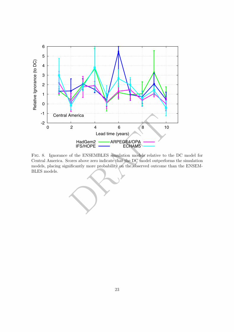
DRAFT

-2

-1

0

1

2

3

4

5

6

0 2 4 6 8 10

Rela

tive

Igno

ranc

e (to

DC)

Lead time (years)

Central America

HadGem2IFS/HOPE

ARPEGE4/OPAECHAM5

Fig. 8. Ignorance of the ENSEMBLES simulation models relative to the DC model forCentral America. Scores above zero indicate that the DC model outperforms the simulationmodels, placing significantly more probability on the observed outcome than the ENSEM-BLES models.

23

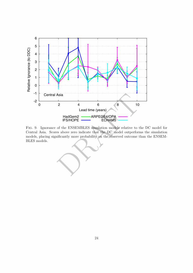
DRAFT

-2

-1

0

1

2

3

4

5

6

0 2 4 6 8 10

Rela

tive

Igno

ranc

e (to

DDC

)

Lead time (years)

Central Asia

HadGem2IFS/HOPE

ARPEGE4/OPAECHAM5

Fig. 9. Ignorance of the ENSEMBLES simulation models relative to the DC model forCentral Asia. Scores above zero indicate that the DC model outperforms the simulationmodels, placing significantly more probability on the observed outcome than the ENSEM-BLES models.

24

DRAFT

-2

-1

0

1

2

3

4

5

6

0 2 4 6 8 10

Rela

tive

Igno

ranc

e (to

DC)

Lead time (years)

Central North America

HadGem2IFS/HOPE

ARPEGE4/OPAECHAM5

Fig. 10. Ignorance of the ENSEMBLES simulation models relative to the DC model forCentral North America. Scores above zero indicate that the DC model outperforms thesimulation models, placing significantly more probability on the observed outcome than theENSEMBLES models.

25

DRAFT

-2

-1

0

1

2

3

4

5

6

0 2 4 6 8 10

Rela

tive

Igno

ranc

e (to

DC)

Lead time (years)

Eastern Africa

HadGem2IFS/HOPE

ARPEGE4/OPAECHAM5

Fig. 11. Ignorance of the ENSEMBLES simulation models relative to the DC model forEastern Africa. Scores above zero indicate that the DC model outperforms the simulationmodels, placing significantly more probability on the observed outcome than the ENSEM-BLES models.

26

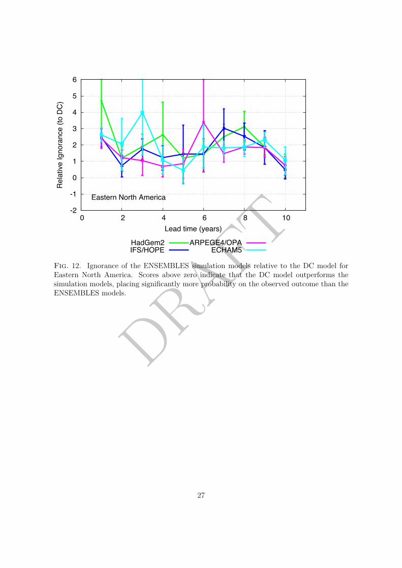
DRAFT

-2

-1

0

1

2

3

4

5

6

0 2 4 6 8 10

Rela

tive

Igno

ranc

e (to

DC)

Lead time (years)

Eastern North America

HadGem2IFS/HOPE

ARPEGE4/OPAECHAM5

Fig. 12. Ignorance of the ENSEMBLES simulation models relative to the DC model forEastern North America. Scores above zero indicate that the DC model outperforms thesimulation models, placing significantly more probability on the observed outcome than theENSEMBLES models.

27

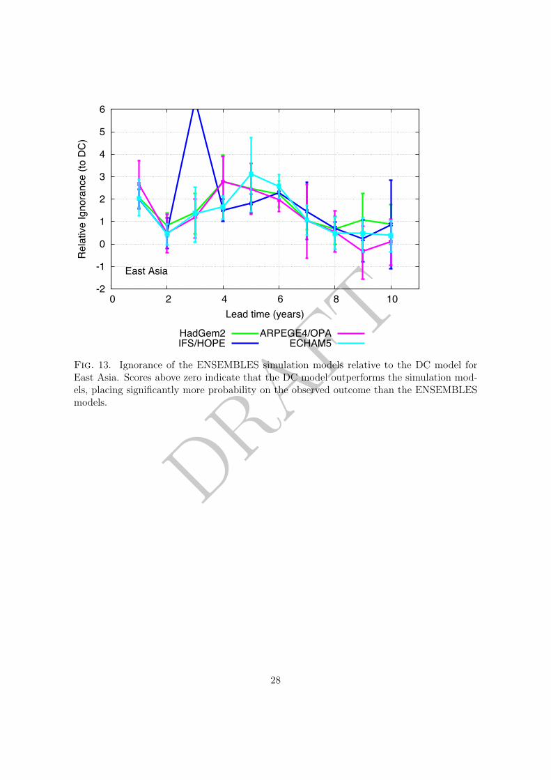
DRAFT

-2

-1

0

1

2

3

4

5

6

0 2 4 6 8 10

Rela

tive

Igno

ranc

e (to

DC)

Lead time (years)

East Asia

HadGem2IFS/HOPE

ARPEGE4/OPAECHAM5

Fig. 13. Ignorance of the ENSEMBLES simulation models relative to the DC model forEast Asia. Scores above zero indicate that the DC model outperforms the simulation mod-els, placing significantly more probability on the observed outcome than the ENSEMBLESmodels.

28

DRAFT

-2

-1

0

1

2

3

4

5

6

0 2 4 6 8 10

Rela

tive

Igno

ranc

e (to

DC)

Lead time (years)

Greenland

HadGem2IFS/HOPE

ARPEGE4/OPAECHAM5

Fig. 14. Ignorance of the ENSEMBLES simulation models relative to the DC model forGreenland. Scores above zero indicate that the DC model outperforms the simulation mod-els, placing significantly more probability on the observed outcome than the ENSEMBLESmodels.

29

DRAFT

-2

-1

0

1

2

3

4

5

6

0 2 4 6 8 10

Rela

tive

Igno

ranc

e (to

DC)

Lead time (years)

Mediterranian Basin

HadGem2IFS/HOPE

ARPEGE4/OPAECHAM5

Fig. 15. Ignorance of the ENSEMBLES simulation models relative to the DC model forMediterranian Basin. Scores above zero indicate that the DC model outperforms the sim-ulation models, placing significantly more probability on the observed outcome than theENSEMBLES models.

30

DRAFT

-2

-1

0

1

2

3

4

5

6

0 2 4 6 8 10

Rela

tive

Igno

ranc

e (to

DC)

Lead time (years)

North Asia

HadGem2IFS/HOPE

ARPEGE4/OPAECHAM5

Fig. 16. Ignorance of the ENSEMBLES simulation models relative to the DC model forNorth Asia. Scores above zero indicate that the DC model outperforms the simulation mod-els, placing significantly more probability on the observed outcome than the ENSEMBLESmodels.

31

DRAFT

-2

-1

0

1

2

3

4

5

6

0 2 4 6 8 10

Rela

tive

Igno

ranc

e (to

DC)

Lead time (years)

Northern Europe

HadGem2IFS/HOPE

ARPEGE4/OPAECHAM5

Fig. 17. Ignorance of the ENSEMBLES simulation models relative to the DC model forNorthern Europe. Scores above zero indicate that the DC model outperforms the simulationmodels, placing significantly more probability on the observed outcome than the ENSEM-BLES models.

32

DRAFT

-2

-1

0

1

2

3

4

5

6

0 2 4 6 8 10

Rela

tive

Igno

ranc

e (to

DC)

Lead time (years)

Southern Africa

HadGem2IFS/HOPE

ARPEGE4/OPAECHAM5

Fig. 18. Ignorance of the ENSEMBLES simulation models relative to the DC model forSouthern Africa. Scores above zero indicate that the DC model outperforms the simulationmodels, placing significantly more probability on the observed outcome than the ENSEM-BLES models.

33

DRAFT

-2

-1

0

1

2

3

4

5

6

0 2 4 6 8 10

Rela

tive

Igno

ranc

e (to

DC)

Lead time (years)

Sahara

HadGem2IFS/HOPE

ARPEGE4/OPAECHAM5

Fig. 19. Ignorance of the ENSEMBLES simulation models relative to the DC model forSahara. Scores above zero indicate that the DC model outperforms the simulation mod-els, placing significantly more probability on the observed outcome than the ENSEMBLESmodels.

34

DRAFT

-2

-1

0

1

2

3

4

5

6

0 2 4 6 8 10

Rela

tive

Igno

ranc

e (to

DC)

Lead time (years)

South Asia

HadGem2IFS/HOPE

ARPEGE4/OPAECHAM5

Fig. 20. Ignorance of the ENSEMBLES simulation models relative to the DC model forSouth Asia. Scores above zero indicate that the DC model outperforms the simulation mod-els, placing significantly more probability on the observed outcome than the ENSEMBLESmodels.

35

DRAFT

-2

-1

0

1

2

3

4

5

6

0 2 4 6 8 10

Rela

tive

Igno

ranc

e (to

DC)

Lead time (years)

Southeast Asia

HadGem2IFS/HOPE

ARPEGE4/OPAECHAM5

Fig. 21. Ignorance of the ENSEMBLES simulation models relative to the DC model forSoutheast Asia. Scores above zero indicate that the DC model outperforms the simulationmodels, placing significantly more probability on the observed outcome than the ENSEM-BLES models.

36

DRAFT

-2

-1

0

1

2

3

4

5

6

0 2 4 6 8 10

Rela

tive

Igno

ranc

e (to

DC)

Lead time (years)

Southern South America

HadGem2IFS/HOPE

ARPEGE4/OPAECHAM5

Fig. 22. Ignorance of the ENSEMBLES simulation models relative to the DC model forSouthern South America. Scores above zero indicate that the DC model outperforms thesimulation models, placing significantly more probability on the observed outcome than theENSEMBLES models.

37

DRAFT

-2

-1

0

1

2

3

4

5

6

0 2 4 6 8 10

Rela

tive

Igno

ranc

e (to

DC)

Lead time (years)

Tibet

HadGem2IFS/HOPE

ARPEGE4/OPAECHAM5

Fig. 23. Ignorance of the ENSEMBLES simulation models relative to the DC model forTibet. Scores above zero indicate that the DC model outperforms the simulation mod-els, placing significantly more probability on the observed outcome than the ENSEMBLESmodels.

38

DRAFT

-2

-1

0

1

2

3

4

5

6

0 2 4 6 8 10

Rela

tive

Igno

ranc

e (to

DC)

Lead time (years)

Western Africa

HadGem2IFS/HOPE

ARPEGE4/OPAECHAM5

Fig. 24. Ignorance of the ENSEMBLES simulation models relative to the DC model forWestern Africa. Scores above zero indicate that the DC model outperforms the simulationmodels, placing significantly more probability on the observed outcome than the ENSEM-BLES models.

39

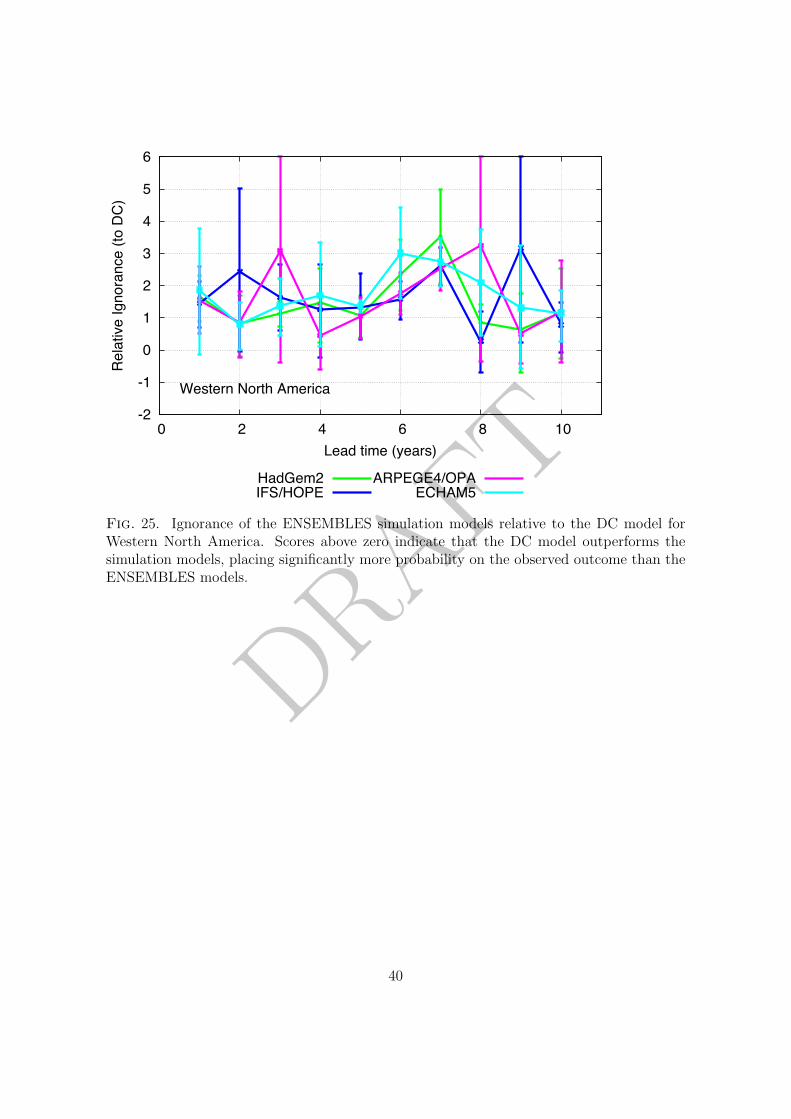
DRAFT

-2

-1

0

1

2

3

4

5

6

0 2 4 6 8 10

Rela

tive

Igno

ranc

e (to

DC)

Lead time (years)

Western North America

HadGem2IFS/HOPE

ARPEGE4/OPAECHAM5

Fig. 25. Ignorance of the ENSEMBLES simulation models relative to the DC model forWestern North America. Scores above zero indicate that the DC model outperforms thesimulation models, placing significantly more probability on the observed outcome than theENSEMBLES models.

40

DRAFT-0.003

-0.0025

-0.002

-0.0015

-0.001

-0.0005

0

0 1 2 3 4 5 6 7 8 9

Prop

er L

inea

r

Lead time (years)

hadgem2IFS/HOPEARPEGE4/OPAECHAM5DC

Fig. 26. Proper linear score for each of the ENSEMBLES simulation models and the DC em-pirical model. Lower scores indicate better foecasts. The DC model is shown to outperformthe simulations models at most lead times.

41

DRAFT 0

100

200

300

400

500

600

700

800

900

1000

0 1 2 3 4 5 6 7 8 9

CRPS

Lead time (years)

hadgem2IFS/HOPEARPEGE4/OPAECHAM5DC

Fig. 27. CRPS score for each of the ENSEMBLES simulation models and the DC empiricalmodel. Lower scores indicate better forecasts. The DC model is shown to outperform thesimulations models at most lead times.

42

DRAFT-0.5

0

0.5

1

1.5

2

2.5

0 2 4 6 8 10

Igno

ranc

e (re

lativ

e to

DC

)

Lead time (years)

Prelaunch DC (sigma=0.02)Prelaunch DC (sigma=0.04)Prelaunch DC (sigma=0.08)Prelaunch DC (sigma=0.16)

Fig. 28. Ignorance of the Prelaunch DC empirical model with kernel widths as labelledrelative to the cross-validation DC model. Increasing the kernel width parameter from 0.02to 0.16 results in a loss of skill of approximately half a bit, although for the kernel widthvalue used in this paper (0.08) there is shown to be no significant loss of skill relative to thestandard DC model.

43

DRAFT

-2

-1.5

-1

-0.5

0

0.5

1

1.5

2

0 0.05 0.1 0.15 0.2

Igno

ranc

e

Kernel width

DC lt1

-2

-1.5

-1

-0.5

0

0.5

1

1.5

2

0 0.05 0.1 0.15 0.2

Igno

ranc

e

Kernel width

Prelaunch DC lt1

-2

-1.5

-1

-0.5

0

0.5

1

1.5

2

0 0.05 0.1 0.15 0.2

Igno

ranc

e

Kernel width

DC lt6

-2

-1.5

-1

-0.5

0

0.5

1

1.5

2

0 0.05 0.1 0.15 0.2

Igno

ranc

e

Kernel width

Prelaunch DC lt6

-2

-1.5

-1

-0.5

0

0.5

1

1.5

2

0 0.05 0.1 0.15 0.2

Igno

ranc

e

Kernel width

DC lt10

-2

-1.5

-1

-0.5

0

0.5

1

1.5

2

0 0.05 0.1 0.15 0.2

Igno

ranc

e

Kernel width

Prelaunch DC lt10

Fig. 29. Ignorance as a function of the kernel width parameter over the full set of hindcastsimulations (i.e. with no cross-validation) for the DC (left panels) and Prelaunch DC (rightpanels) models at lead time one (a and b), six (c and d) and ten (e and f). The vertical barsin each case illustrate the kernel width parameters employed in the main manuscript. Inthe DC model parameters were attained through true-leave-one-out cross-validation. In thePrelaunch DC model a kernel spread value of 0.08 was chosen for comparison with DC andto test the robustness of the results to choices in the parameters for ensemble interpretation(although this value does not correspond to the lowest value of in-sample skill).

44

DRAFT-0.5

0

0.5

1

1.5

2

2.5

0 2 4 6 8 10

Igno

ranc

e (re

lativ

e to

DC

)

Lead time (years)

Prelaunch Trend (1900 anchor)Prelaunch Trend (1925 anchor)Prelaunch Trend (1940 anchor)Prelaunch Trend (1950 anchor)

Fig. 30. Ignorance of the Prelaunch trend empirical model for di!erent anchor times relativeto the cross-validation DC model. Scores above zero indicate that DC outperforms thePrelaunch Trend model by up to half a bit at early lead times, and up to two bits (DCplacing up to 4 times more probability on the observed outcome than the Prelaunch Trendmodel) up to ten years ahead, depending on the anchor year for the trend model.

45