An Evaluation of Tropical Cyclone Genesis Forecasts from...

An Evaluation of Tropical Cyclone Genesis Forecasts from Global Numerical Models

DANIEL J. HALPERIN, HENRY E. FUELBERG, ROBERT E. HART, JOSHUA H. COSSUTH,AND PHILIP SURA

The Florida State University, Tallahassee, Florida

RICHARD J. PASCH

National Hurricane Center, Miami, Florida

(Manuscript received 11 January 2013, in final form 28 March 2013)

ABSTRACT

Tropical cyclone (TC) forecasts rely heavily on output from global numerical models. While considerable

research has investigated the skill of various models with respect to track and intensity, few studies have con-

sidered how well global models forecast TC genesis in the NorthAtlantic basin. This paper analyzes TC genesis

forecasts from five global models [Environment Canada’s Global Environment Multiscale Model (CMC), the

European Centre forMedium-RangeWeather Forecasts (ECMWF) global model, the Global Forecast System

(GFS), the Navy Operational Global Atmospheric Prediction System (NOGAPS), and the Met Office global

model (UKMET)] over several seasons in the North Atlantic basin. Identifying TCs in the model is based on

a combination of methods used previously in the literature and newly defined objective criteria. All model-

indicated TCs are classified as a hit, false alarm, early genesis, or late genesis event. Missed events also are

considered. Results show that the models’ ability to predict TC genesis varies in time and space. Conditional

probabilities when a model predicts genesis and more traditional performance metrics (e.g., critical success

index) are calculated. The models are ranked among each other, and results show that the best-performing

model varies from year to year. A spatial analysis of each model identifies preferred regions for genesis, and

a temporal analysis indicates that model performance expectedly decreases as forecast hour (lead time) in-

creases. Consensus forecasts show that the probability of genesis noticeably increases when multiple models

predict the same genesis event. Overall, this study provides a climatology of objectively identified TC genesis

forecasts in global models. The resulting verification statistics can be used operationally to help refine de-

terministic and probabilistic TC genesis forecasts and potentially improve the models examined.

1. Introduction

Human forecasts of tropical cyclones (TCs) rely

greatly on numerical models. Each model used by

forecasters at the National Hurricane Center (NHC) has

unique strengths and weaknesses. Research has in-

vestigated the skill of these models with respect to track

and intensity, with the assumption that a TC already

exists (e.g., Goerss 2000; Goerss et al. 2004; Sampson

et al. 2008). Several studies have investigated global

models’ ability to predict TC genesis at various lead times

in the western North Pacific (WNP) basin using various

models and periods of study (e.g., Briegel and Frank 1997;

Chan andKwok1999;Cheung andElsberry 2002; Elsberry

et al. 2009, 2010, 2011; Tsai et al. 2011). However, in-

sufficient research has focused on the skill of model fore-

casts of TC genesis in the North Atlantic (NATL) basin.

The goal of this study is to quantify the accuracy of

model-indicated TC genesis through 96 h in the NATL

basin. Specifically, we are interested in analyzing the

relative performance of multiple global models. Thus,

we compare results from Environment Canada’s Global

Environmental Multiscale Model (CMC; Cot�e et al.

1998a,b), the European Centre for Medium-Range

Weather Forecasts global model (ECMWF 2012), the

National Centers for Environmental Prediction (NCEP)

Global Forecast System (GFS; Kanamitsu 1989), the

NavyOperationalGlobalAtmospheric Prediction System

(NOGAPS; Rosmond 1992), and the Met Office global

Corresponding author address: Daniel J. Halperin, Dept. of

Earth, Ocean, and Atmospheric Science, The Florida State Uni-

versity, Tallahassee, FL 32306-4520.

E-mail: [email protected]

DECEMBER 2013 HALPER IN ET AL . 1423

DOI: 10.1175/WAF-D-13-00008.1

� 2013 American Meteorological Society

mailto:[email protected]

model (UKMET; Cullen 1993). These forecasts are veri-

fied against the genesis of best-track (BT; Jarvinen et al.

1984; McAdie et al. 2009) TCs.

Each year approximately 80–90 TCs develop globally

(Frank and Young 2007). This paper focuses on the

NATL given its relevance to theNHC, but the algorithm

employed can be applied globally in the future to assist

other operational centers. Tory and Frank (2010) list

five conditions that are necessary for TC genesis based

on a revision of Gray’s (1968) first global TC genesis

climatology:

‘‘1) Sea surface temperatures (SST) above 26.58–278Ccoupled with a relatively deep oceanic mixed layer

(;50m) [it should be noted that recent genesis

potential indices (e.g., Emanuel and Nolan 2004;

Camargo et al. 2007) have abandoned SST in favor

of the more theoretically justified potential inten-

sity (Emanuel 1988)];

2) a deep surface-based layer of conditional instability;

3) enhanced values of cyclonic low-level absolute

vorticity;

4) organized deep convection in an area with large-

scale mean ascent and high midlevel humidity; and

5) weak to moderate (preferably easterly) vertical

wind shear.’’

The entirety of the processes that cause TC genesis

still is largely unknown. This is evident by the number of

TC genesis theories that have been proposed, and the

disagreement that exists among them. One of the oldest

theories is Charney and Eliassen’s (1964) conditional

instability of the second kind (CISK), which since has

been largely disproved as a mechanism for TC develop-

ment (Craig and Gray 1996). Emanuel (1986) proposed

wind-induced surface heat exchange (WISHE), which,

while a more accepted theory for steady-state TCs, has

deficiencies for explaining genesis (Craig and Gray 1996;

Montgomery et al. 2009). Ritchie andHolland (1997) and

Simpson et al. (1997) were the initial proponents of the

‘‘top down’’ TC genesis theory. There also is a ‘‘bottom

up’’ theory proposed by Montgomery and Enagonio

(1998) and Enagonio and Montgomery (2001). A more

recent TC genesis theory is proposed by Dunkerton et al.

(2008). Several field experiments [e.g., Pre-Depression

Investigation ofCloud-Systems in theTropics (PREDICT;

Montgomery et al. 2012), Genesis and Rapid Intensi-

fication Processes (GRIP; Braun et al. 2013), Intensity

Forecasting Experiment (IFEX;Rogers et al. 2006)] have

been conducted to evaluate these theories, but results

have not yet yielded an entire understanding of the pro-

cesses that cause TC genesis.

The operational models are not bound by the above-

mentioned theories or the conditions stated to be

necessary for TC development; thus, they may not pre-

dict development based on physically accepted reasons.

Also, due to grid spacing and computational limitations,

the models are not able to resolve all of the atmospheric

processes governed by the full Navier–Stokes equations.

For example, convection, planetary boundary layer

processes, and microphysical processes all are parame-

terized. Therefore, one cannot expect the models to

fully resolve all of the processes that are necessary for

TC genesis. Despite the above caveats, the models

commonly indicate TC-like development in the forecast

fields (e.g., Pasch et al. 2006, 2008).

While much time and resources have been devoted to

improving model-derived TC track and intensity fore-

casts, the literature contains relatively few assessments

of the models’ ability to predict TC genesis in the NATL

basin or determine what model enhancements should be

made to improve that prediction. Several modes of de-

velopment exist in the NATL basin (McTaggart-Cowan

et al. 2008): nonbaroclinic (40%), low-level baroclinic

(13%), transient-trough interaction (16%), trough in-

duced (3%), weak tropical transition (13%), and strong

tropical transition (15%). In addition, the significance of

factors driving development varies from month to

month. For example, TCs forming fromAfrican easterly

waves (AEWs) are most prevalent from August to mid-

September (Gray 1968). Because of this variability, ‘‘the

North Atlantic is the most complicated development

region’’ (Gray 1968).

Early investigations of model TC genesis forecasts in

the NATL indicated that while the models sometimes

accurately predict TC genesis, they frequently generate

TCs that do not develop (Beven 1999). Conversely, a TC

sometimes develops that has not been forecast in the

models. The relative performance of three global

models (GFS, NOGAPS, UKMET) in predicting TC

genesis was analyzed during the 2005 NATL TC season

(Pasch et al. 2006). Results showed that the GFS had the

greatest probability of detection (POD), but also the

greatest number of false alarms (FAs). Conversely,

NOGAPS exhibited both the smallest POD and the

smallest number of FAs. Pasch et al. (2008) indicated

that the accuracy of TC genesis forecasts varies greatly

from one TC to another. During 2007, the genesis of

Dean (an eventual category 5 hurricane) was well pre-

dicted by the GFS several days in advance. However,

several weeks later, the GFS failed to predict Felix

(another eventual category 5 hurricane).

The current study expands upon these previous works

by analyzing additional models and including additional

TC seasons in the dataset to provide a more robust cli-

matology of model-indicated TC genesis forecasts. It is

important to define metrics for the forecast cases’ varying

1424 WEATHER AND FORECAST ING VOLUME 28

degrees of success. In general the model-indicated fore-

casts can be verified by whether or not TC genesis ac-

tually occurred. But, there are cases where some, but not

all, aspects of the forecast are correct. So, while it is

important to analyze successful forecasts, we must also

examine partially successful forecasts, as well as FA

cases and cases when a TC formed in reality but was

missed by the global models. Hypotheses regarding the

reasons for the analyzed relative performance of the

models are beyond the scope of this paper.

Section 2 describes the datasets and methods that

were used to define, identify, track, and classify each

model-indicated TC as a hit, an FA, or an early genesis

(EG) or a late genesis (LG) event. The results (section 3)

include metrics for evaluating the models’ overall per-

formance as well as geographic and temporal breakdowns

of that performance. The summary and conclusions are

presented in section 4.

2. Methodology

a. Data

A robust analysis of TC genesis forecasts required

a sufficiently large dataset. A local archive of global

operational model data included output from the CMC,

GFS,NOGAPS, andUKMETglobalmodels from 2004 to

2011. ECMWF model output was provided by The Ob-

serving System Research and Predictability Experiment

(THORPEX) Interactive Grand Global Ensemble

(TIGGE) data archive (ECMWF portal) and was avail-

able for the 2007–11 seasons. Table 1 summarizes fea-

tures of each model (B�elair et al. 2009; NHC 2011;

ECMWF 2012; Environmental Modeling Center 2012;

NRL 2012; COMET 2012; J. Heming 2012, personal

communication). Appendix A describes selected up-

grades to each model during the period of study. Since

data were unavailable for some periods, Table 2 shows

start and end dates of the dataset by season and which

TCs and models are not included during the available

time period. The period of study includes some of the

most active NATL hurricane seasons on record. Our

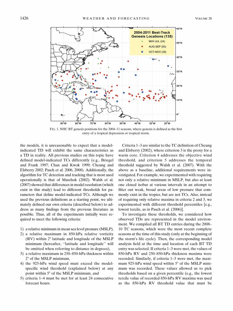
dataset contains 135 BT TC genesis events, with Fig. 1

showing their geographic distribution. TC genesis loca-

tions are defined as the first time that NHCdesignated the

cyclone as a tropical depression (TD) or tropical storm

(TS). For example, the location of tropical cyclogenesis

for Vince (2005) is different than the location when ad-

visories were initiated because Vince initially was a sub-

tropical cyclone. Storms that were subtropical throughout

their entire life cycle were not considered.

b. Definition of model TC

An important component of this research was to de-

fine a model-simulated TC. Given the number of pro-

cesses that are parameterized in the models due to

resolution and computational limitations and the limited

number of in situ observations that are assimilated into

TABLE 1. Summary of model characteristics (B�elair et al. 2009; NHC 2011; ECMWF 2012; Environmental Modeling Center 2012; NRL

2012; COMET 2012; J. Heming 2012, personal communication).

Model Model physics

Native horizontal

grid spacing (km)

Vertical

levels Vertical coordinates Data assimilation

CMC Hydrostatic grid point ;33 80 Hybrid sigma pressure 4DVAR

ECMWF Hydrostatic spectral ;16 91 Hybrid sigma pressure 4DVAR

GFS Hydrostatic spectral ;27 64 Hybrid sigma pressure 3DVAR; GSI/Global Data Assimilation

System (GDAS) analysis

NOGAPS Hydrostatic spectral ;42 42 Hybrid sigma pressure 4DVAR; NAVDAS analysis

UKMET Nonhydrostatic grid point ;25 70 Hybrid sigma pressure Hybrid

TABLE 2. Date ranges of model output in the dataset. Storms andmodels not included in the dataset are listed. The dataset contains 135 storms.

Year Date range Storms not included in dataset Models not included in dataset

2004 20 Jul–30 Nov Nicole ECMWF

2005 7 May–30 Nov Unnamed subtropical storm,

subtropical depression 22, Zeta

ECMWF

2006 6 Jun–30 Nov None ECMWF

2007 21 May–30 Nov Andrea, Olga None

2008 31 May–30 Nov Arthur, Laura None

2009 18 May–30 Nov None None

2010 8 Jun–9 Nov None None

2011 1 Jun–30 Nov None None


the models, it is unreasonable to expect that a model-

indicated TD will exhibit the same characteristics as

a TD in reality. All previous studies on this topic have

defined model-indicated TCs differently (e.g., Briegel

and Frank 1997; Chan and Kwok 1999; Cheung and

Elsberry 2002; Pasch et al. 2006, 2008). Additionally, the

algorithm for TC detection and tracking that is most used

operationally is that of Marchok (2002). Walsh et al.

(2007) showed that differences inmodel resolution (which

exist in this study) lead to different thresholds for pa-

rameters that define model-indicated TCs. Although we

used the previous definitions as a starting point, we ulti-

mately defined our own criteria (described below) to ad-

dress as many findings from the previous literature as

possible. Thus, all of the experiments initially were re-

quired to meet the following criteria:

1) a relativeminimum inmean sea level pressure (MSLP),

2) a relative maximum in 850-hPa relative vorticity

(RV) within 28 latitude and longitude of the MSLP

minimum (hereafter, ‘‘latitude and longitude’’ will

be omitted when referring to distance in degrees),

3) a relative maximum in 250–850-hPa thickness within

28 of the MSLP minimum,

4) the 925-hPa wind speed must exceed the model-

specific wind threshold (explained below) at any

point within 58 of the MSLP minimum, and

5) criteria 1–4 must be met for at least 24 consecutive

forecast hours.

Criteria 1–3 are similar to the TC definition of Cheung

and Elsberry (2002), where criterion 3 is the proxy for a

warm core. Criterion 4 addresses the objective wind

threshold, and criterion 5 addresses the temporal

threshold suggested by Walsh et al. (2007). With the

above as a baseline, additional requirements were in-

vestigated. For example, we experimented with requiring

not only a relative minimum in MSLP, but also at least

one closed isobar at various intervals in an attempt to

filter out weak, broad areas of low pressure that com-

monly exist in the tropics, but are not TCs. Also, instead

of requiring only relative maxima in criteria 2 and 3, we

experimented with different threshold percentiles [e.g.,

lowest tercile, as in Pasch et al. (2006)].

To investigate these thresholds, we considered how

observed TDs are represented in the model environ-

ment. We compiled all BT TD entries during the 2008–

10 TC seasons, which were the most recent complete

seasons at the time of this study (only at the beginning of

the storm’s life cycle). Then, the corresponding model

analysis field at the time and location of each BT TD

entry was selected. If criteria 1–3 were met, the values of

850-hPa RV and 250–850-hPa thickness maxima were

recorded. Similarly, if criteria 1–3 were met, the maxi-

mum 925-hPa wind speed within 58 of the MSLP mini-

mum was recorded. These values allowed us to pick

thresholds based on a given percentile (e.g., the lowest

tercile value of recorded 850-hPa RV maxima was used

as the 850-hPa RV threshold value that must be

FIG. 1. NHC BT genesis positions for the 2004–11 seasons, where genesis is defined as the first

entry of a tropical depression or tropical storm.


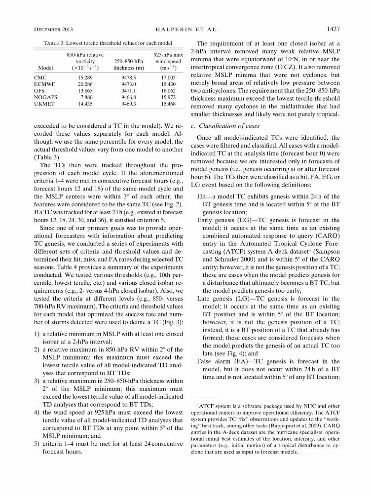
exceeded to be considered a TC in the model). We re-

corded these values separately for each model. Al-

though we use the same percentile for every model, the

actual threshold values vary from one model to another

(Table 3).

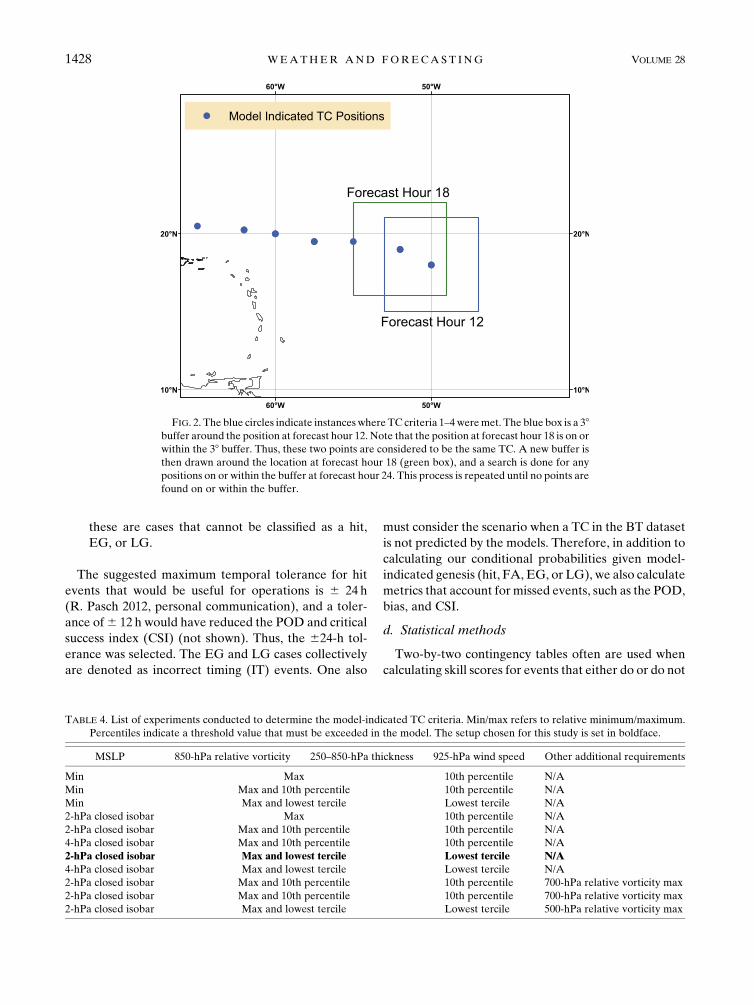
The TCs then were tracked throughout the pro-

gression of each model cycle. If the aforementioned

criteria 1–4 were met in consecutive forecast hours (e.g.,

forecast hours 12 and 18) of the same model cycle and

the MSLP centers were within 38 of each other, the

features were considered to be the same TC (see Fig. 2).

If a TCwas tracked for at least 24h (e.g., existed at forecast

hours 12, 18, 24, 30, and 36), it satisfied criterion 5.

Since one of our primary goals was to provide oper-

ational forecasters with information about predicting

TC genesis, we conducted a series of experiments with

different sets of criteria and threshold values and de-

termined their hit, miss, and FA rates during selected TC

seasons. Table 4 provides a summary of the experiments

conducted. We tested various thresholds (e.g., 10th per-

centile, lowest tercile, etc.) and various closed isobar re-

quirements (e.g., 2- versus 4-hPa closed isobar). Also, we

tested the criteria at different levels (e.g., 850- versus

700-hPaRVmaximum). The criteria and threshold values

for each model that optimized the success rate and num-

ber of storms detected were used to define a TC (Fig. 3):

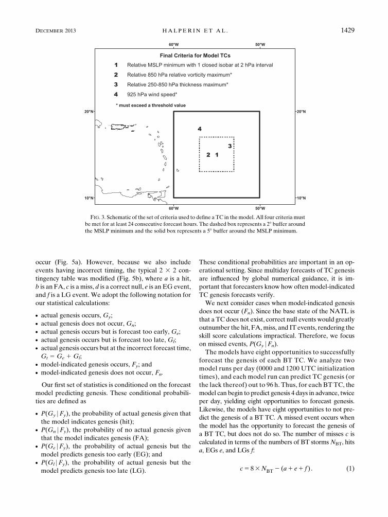
1) a relative minimum in MSLP with at least one closed

isobar at a 2-hPa interval;

2) a relative maximum in 850-hPa RV within 28 of theMSLP minimum; this maximum must exceed the

lowest tercile value of all model-indicated TD anal-

yses that correspond to BT TDs;

3) a relative maximum in 250–850-hPa thickness within

28 of the MSLP minimum; this maximum must

exceed the lowest tercile value of all model-indicated

TD analyses that correspond to BT TDs;

4) the wind speed at 925 hPa must exceed the lowest

tercile value of all model-indicated TD analyses that

correspond to BT TDs at any point within 58 of theMSLP minimum; and

5) criteria 1–4 must be met for at least 24 consecutive

forecast hours.

The requirement of at least one closed isobar at a

2-hPa interval removed many weak relative MSLP

minima that were equatorward of 108N, in or near the

intertropical convergence zone (ITCZ). It also removed

relative MSLP minima that were not cyclones, but

merely broad areas of relatively low pressure between

two anticyclones. The requirement that the 250–850-hPa

thickness maximum exceed the lowest tercile threshold

removed many cyclones in the midlatitudes that had

smaller thicknesses and likely were not purely tropical.

c. Classification of cases

Once all model-indicated TCs were identified, the

cases were filtered and classified. All cases with a model-

indicated TC at the analysis time (forecast hour 0) were

removed because we are interested only in forecasts of

model genesis (i.e., genesis occurring at or after forecast

hour 6). The TCs thenwere classified as a hit, FA, EG, or

LG event based on the following definitions:

Hit—a model TC exhibits genesis within 24 h of the

BT genesis time and is located within 58 of the BT

genesis location;

Early genesis (EG)—TC genesis is forecast in the

model; it occurs at the same time as an existing

combined automated response to query (CARQ)

entry in the Automated Tropical Cyclone Fore-

casting (ATCF) system A-deck dataset1 (Sampson

and Schrader 2000) and is within 58 of the CARQ

entry; however, it is not the genesis position of a TC;

these are cases when the model predicts genesis for

a disturbance that ultimately becomes a BT TC, but

the model predicts genesis too early;

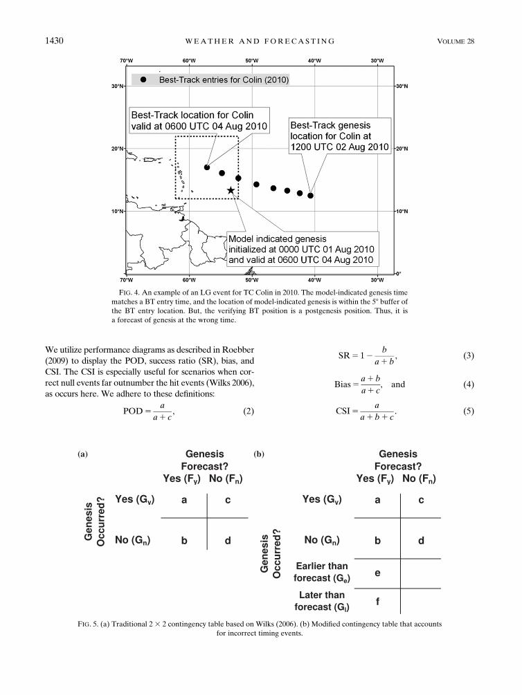
Late genesis (LG)—TC genesis is forecast in the

model; it occurs at the same time as an existing

BT position and is within 58 of the BT location;

however, it is not the genesis position of a TC;

instead, it is a BT position of a TC that already has

formed; these cases are considered forecasts when

the model predicts the genesis of an actual TC too

late (see Fig. 4); and

False alarm (FA)—TC genesis is forecast in the

model, but it does not occur within 24 h of a BT

time and is not located within 58 of any BT location;

TABLE 3. Lowest tercile threshold values for each model.

Model

850-hPa relative

vorticity

(31025 s21)

250–850-hPa

thickness (m)

925-hPa max

wind speed

(m s21)

CMC 15.289 9478.5 17.005

ECMWF 20.286 9473.0 15.430

GFS 13.865 9471.1 16.062

NOGAPS 7.880 9466.8 15.972

UKMET 14.435 9469.3 15.468

1ATCF system is a software package used by NHC and other

operational centers to improve operational efficiency. The ATCF

system provides TC ‘‘fix’’ observations and updates to the ‘‘work-

ing’’ best track, among other tasks (Rappaport et al. 2009). CARQ

entries in the A-deck dataset are the hurricane specialists’ opera-

tional initial best estimates of the location, intensity, and other

parameters (e.g., initial motion) of a tropical disturbance or cy-

clone that are used as input to forecast models.


these are cases that cannot be classified as a hit,

EG, or LG.

The suggested maximum temporal tolerance for hit

events that would be useful for operations is 6 24 h

(R. Pasch 2012, personal communication), and a toler-

ance of6 12 h would have reduced the POD and critical

success index (CSI) (not shown). Thus, the 624-h tol-

erance was selected. The EG and LG cases collectively

are denoted as incorrect timing (IT) events. One also

must consider the scenario when a TC in the BT dataset

is not predicted by the models. Therefore, in addition to

calculating our conditional probabilities given model-

indicated genesis (hit, FA, EG, or LG), we also calculate

metrics that account for missed events, such as the POD,

bias, and CSI.

d. Statistical methods

Two-by-two contingency tables often are used when

calculating skill scores for events that either do or do not

FIG. 2. The blue circles indicate instanceswhere TC criteria 1–4weremet. The blue box is a 38buffer around the position at forecast hour 12. Note that the position at forecast hour 18 is on or

within the 38 buffer. Thus, these two points are considered to be the same TC. A new buffer is

then drawn around the location at forecast hour 18 (green box), and a search is done for any

positions on or within the buffer at forecast hour 24. This process is repeated until no points are

found on or within the buffer.

TABLE 4. List of experiments conducted to determine the model-indicated TC criteria. Min/max refers to relative minimum/maximum.

Percentiles indicate a threshold value that must be exceeded in the model. The setup chosen for this study is set in boldface.

MSLP 850-hPa relative vorticity 250–850-hPa thickness 925-hPa wind speed Other additional requirements

Min Max 10th percentile N/A

Min Max and 10th percentile 10th percentile N/A

Min Max and lowest tercile Lowest tercile N/A

2-hPa closed isobar Max 10th percentile N/A

2-hPa closed isobar Max and 10th percentile 10th percentile N/A

4-hPa closed isobar Max and 10th percentile 10th percentile N/A

2-hPa closed isobar Max and lowest tercile Lowest tercile N/A

4-hPa closed isobar Max and lowest tercile Lowest tercile N/A

2-hPa closed isobar Max and 10th percentile 10th percentile 700-hPa relative vorticity max

2-hPa closed isobar Max and 10th percentile 10th percentile 700-hPa relative vorticity max

2-hPa closed isobar Max and lowest tercile Lowest tercile 500-hPa relative vorticity max


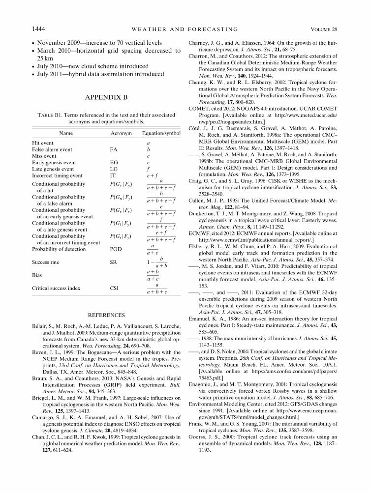
occur (Fig. 5a). However, because we also include

events having incorrect timing, the typical 2 3 2 con-

tingency table was modified (Fig. 5b), where a is a hit,

b is an FA, c is a miss, d is a correct null, e is an EG event,

and f is a LG event. We adopt the following notation for

our statistical calculations:

d actual genesis occurs, Gy;d actual genesis does not occur, Gn;d actual genesis occurs but is forecast too early, Ge;d actual genesis occurs but is forecast too late, Gl;d actual genesis occurs but at the incorrect forecast time,

Gt 5 Ge 1 Gl;d model-indicated genesis occurs, Fy; andd model-indicated genesis does not occur, Fn.

Our first set of statistics is conditioned on the forecast

model predicting genesis. These conditional probabili-

ties are defined as

d P(Gy jFy), the probability of actual genesis given that

the model indicates genesis (hit);d P(Gn jFy), the probability of no actual genesis given

that the model indicates genesis (FA);d P(Ge jFy), the probability of actual genesis but the

model predicts genesis too early (EG); andd P(Gl jFy), the probability of actual genesis but the

model predicts genesis too late (LG).

These conditional probabilities are important in an op-

erational setting. Since multiday forecasts of TC genesis

are influenced by global numerical guidance, it is im-

portant that forecasters know how often model-indicated

TC genesis forecasts verify.

We next consider cases when model-indicated genesis

does not occur (Fn). Since the base state of the NATL is

that a TC does not exist, correct null events would greatly

outnumber the hit, FA,miss, and IT events, rendering the

skill score calculations impractical. Therefore, we focus

on missed events, P(Gy jFn).

The models have eight opportunities to successfully

forecast the genesis of each BT TC. We analyze two

model runs per day (0000 and 1200 UTC initialization

times), and each model run can predict TC genesis (or

the lack thereof) out to 96 h. Thus, for each BT TC, the

model can begin to predict genesis 4 days in advance, twice

per day, yielding eight opportunities to forecast genesis.

Likewise, the models have eight opportunities to not pre-

dict the genesis of a BT TC. A missed event occurs when

the model has the opportunity to forecast the genesis of

a BT TC, but does not do so. The number of misses c is

calculated in terms of the numbers of BT stormsNBT, hits

a, EGs e, and LGs f:

c5 83NBT 2 (a1 e1 f ) . (1)

FIG. 3. Schematic of the set of criteria used to define a TC in the model. All four criteria must

be met for at least 24 consecutive forecast hours. The dashed box represents a 28 buffer aroundthe MSLP minimum and the solid box represents a 58 buffer around the MSLP minimum.


We utilize performance diagrams as described in Roebber

(2009) to display the POD, success ratio (SR), bias, and

CSI. The CSI is especially useful for scenarios when cor-

rect null events far outnumber the hit events (Wilks 2006),

as occurs here. We adhere to these definitions:

POD5a

a1 c, (2)

SR5 12b

a1 b, (3)

Bias5a1 b

a1 c, and (4)

CSI5a

a1b1 c. (5)

FIG. 4. An example of an LG event for TC Colin in 2010. The model-indicated genesis time

matches a BT entry time, and the location of model-indicated genesis is within the 58 buffer ofthe BT entry location. But, the verifying BT position is a postgenesis position. Thus, it is

a forecast of genesis at the wrong time.

FIG. 5. (a) Traditional 23 2 contingency table based on Wilks (2006). (b) Modified contingency table that accounts

for incorrect timing events.


We analyze model performance in two ways: 1) the

aforementioned conditional probabilities, which are

the most useful information in a real-time setting, and

2) the traditional metrics on the performance diagram

(POD, SR, bias, CSI), which provide anoverall description

of model performance and highlight where strengths and

deficiencies exist. For reference, appendix B includes a list

of the statistical terminology and corresponding acronyms

and equations/symbols.

3. Results

We present results for each model separately, calcu-

lating the yearly conditional probability of each event

type given that model-indicated genesis occurs (e.g.,

Fig. 6). This metric provides insight into how often TC

genesis forecasts verify versus how often no TC devel-

ops. We then plot the events on a performance diagram

(e.g., Fig. 7), which efficiently depicts several traditional

success metrics in one figure. Each event also is plotted

geographically (e.g., Fig. 8). We can use the geographic

distribution of genesis events to determine a model’s pre-

ferred genesis region(s). Finally, we calculate the con-

ditional probability of each event type by forecast hour

(e.g., Fig. 9) to show how the reliability of TC genesis

forecasts evolves with time during the model cycle.

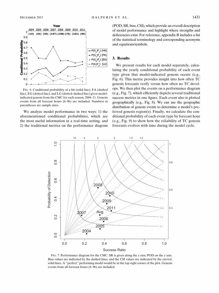
FIG. 6. Conditional probability of a hit (solid line), FA (dashed

line), EG (dotted line), and LG (dotted–dashed line) given model-

indicated genesis from the CMC for each season, 2004–11. Genesis

events from all forecast hours (6–96) are included. Numbers in

parentheses are sample sizes.

FIG. 7. Performance diagram for the CMC. SR is given along the x axis; POD on the y axis.

Bias values are indicated by the dashed lines, and the CSI values are indicated by the curved,

solid lines. A ‘‘perfect’’ performing model would be in the top-right corner of the plot. Genesis

events from all forecast hours (6–96) are included.


a. CMC

Figure 6 shows the yearly conditional probability of

a hit, FA, EG, and LGgiven thatmodel-indicated genesis

occurs. Since 2007, P(Gy jFy) has increased, reaching its

greatest seasonal value of 0.38 in 2011. FAs have been an

issue, but improvements have occurred recently.

The performance diagram for the CMC (Fig. 7) re-

veals that the model predicted TC genesis rather ag-

gressively during 2007 and 2008, likely due to a model

upgrade in late 2006 when the horizontal grid spacing

was changed from 100 to 33 km, the vertical resolution

was increased from 28 to 58 levels, and changes to the

convective schemes were made (B�elair et al. 2009). Bias

values exceeding 1 and SR values less than 0.4 indicate

that many of these genesis events were FAs. Improve-

ments began in 2009, with SR values approaching 0.5 by

2011. The model also became less aggressive in 2011, as

evidenced by the reduced bias (0.94 in 2010 and 0.57 in

2011). The CSI also generally has improved in recent

years (below 0.13 during 2004–07; above 0.2 during

2008–11).

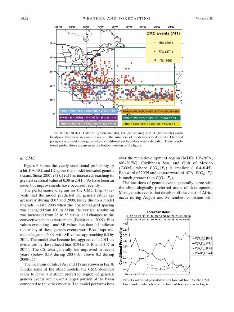
The locations of hits, FAs, and ITs are shown in Fig. 8.

Unlike some of the other models, the CMC does not

seem to have a distinct preferred region of genesis;

genesis events occur over a larger portion of the basin

compared to the other models. The model performs best

over the main development region (MDR; 108–208N,

608–208W), Caribbean Sea, and Gulf of Mexico

(GOM), where P(Gn jFy) is smallest (;0.4–0.45).

Poleward of 208N and equatorward of 108N, P(Gn jFy)

is much greater than P(Gy jFy).

The locations of genesis events generally agree with

the climatologically preferred areas of development.

Most genesis events that develop off the coast of Africa

occur during August and September, consistent with

FIG. 8. The 2004–11 CMC hit (green triangle), FA (red square), and IT (blue circle) event

locations. Numbers in parentheses are the numbers of model-indicated events. Outlined

polygons represent subregions where conditional probabilities were calculated. These condi-

tional probabilities are given in the bottom portion of the figure.

FIG. 9. Conditional probabilities by forecast hour for the CMC.

Lines and numbers below the forecast hours are as in Fig. 6.


Gray (1968). However, during June, July, October, and

November, genesis events generally occur closer to

North America (not shown).

Figure 9 depicts the conditional probability of a hit,

FA, EG, and LG by forecast hour. As expected, model

performance decreases with increasing forecast hour.

Approximately 94% of TC genesis events verify as hits

at forecast hour 6, compared to only;14% at forecast

hour 96. Also note the sharp increase in the number of

model-indicated genesis events between forecast

hours 6 and 24. We speculate this may occur because

the model may take several hours of integration be-

fore it is able to spin up a TC in most cases. The in-

creased number of genesis events after forecast hour

24 is sustained throughout the remainder of the fore-

cast period.

b. ECMWF

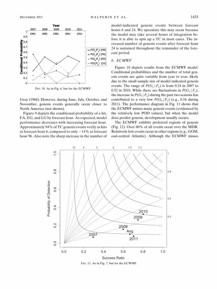
Figure 10 depicts results from the ECMWF model.

Conditional probabilities and the number of total gen-

esis events are quite variable from year to year, likely

due to the small sample size of model-indicated genesis

events. The range of P(Gy jFy) is from 0.24 in 2007 to

0.52 in 2010. While there are fluctuations in P(Gy jFy),

the increase in P(Gt jFy) during the past two seasons has

contributed to a very low P(Gn jFy) (e.g., 0.16 during

2011). The performance diagram in Fig. 11 shows that

the ECMWF misses many genesis events (evidenced by

the relatively low POD values), but when the model

does predict genesis, development usually occurs.

The ECMWF exhibits preferred regions of genesis

(Fig. 12). Over 60% of all events occur over the MDR.

Relatively few events occur in other regions (e.g., GOM,

east-central Atlantic). Although the ECMWF misses

FIG. 10. As in Fig. 6, but for the ECMWF.

FIG. 11. As in Fig. 7, but for the ECWMF.


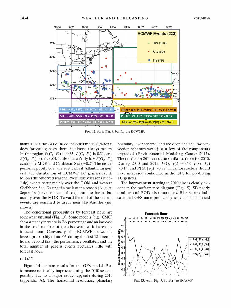
many TCs in the GOM (as do the other models), when it

does forecast genesis there, it almost always occurs.

In this region P(Gy jFy) is 0.65, P(Gt jFy) is 0.31, and

P(Gn jFy) is only 0.04. It also has a fairly low P(Gn jFy)

across the MDR and Caribbean Sea (;0.2). The model

performs poorly over the east-central Atlantic. In gen-

eral, the distribution of ECMWF TC genesis events

follows the observed seasonal cycle. Early season (June–

July) events occur mainly over the GOM and western

Caribbean Sea. During the peak of the season (August/

September) events occur throughout the basin, but

mainly over the MDR. Toward the end of the season,

events are confined to areas near the Antilles (not

shown).

The conditional probabilities by forecast hour are

somewhat unusual (Fig. 13). Some models (e.g., CMC)

show a steady increase in FA percentage and an increase

in the total number of genesis events with increasing

forecast hour. Conversely, the ECMWF shows the

lowest probability of an FA during the first 18 forecast

hours; beyond that, the performance oscillates, and the

total number of genesis events fluctuates little with

forecast hour.

c. GFS

Figure 14 contains results for the GFS model. Per-

formance noticeably improves during the 2010 season,

possibly due to a major model upgrade during 2010

(appendix A). The horizontal resolution, planetary

boundary layer scheme, and the deep and shallow con-

vection schemes were just a few of the components

upgraded (Environmental Modeling Center 2012).

The results for 2011 are quite similar to those for 2010.

During 2010 and 2011, P(Gy jFy) ;0.48, P(Gt jFy)

;0.14, and P(Gn jFy) ;0.38. Thus, forecasters should

have increased confidence in the GFS for predicting

TC genesis.

The improvement starting in 2010 also is clearly evi-

dent in the performance diagram (Fig. 15). SR nearly

doubles and POD also increases. Bias scores indi-

cate that GFS underpredicts genesis and that missed




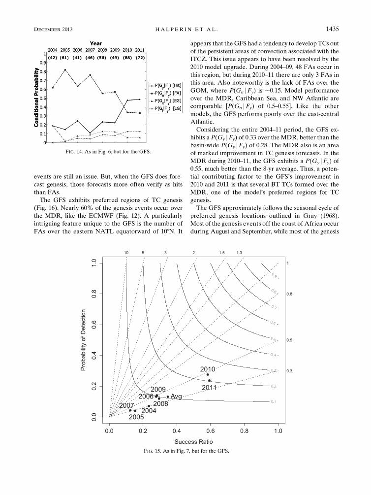
events are still an issue. But, when the GFS does fore-

cast genesis, those forecasts more often verify as hits

than FAs.

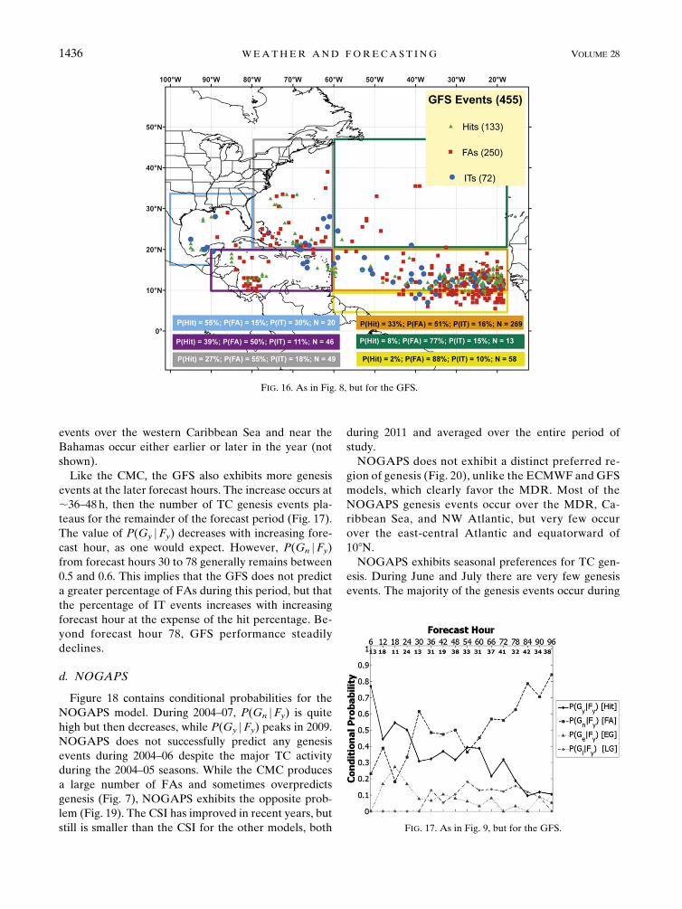
The GFS exhibits preferred regions of TC genesis

(Fig. 16). Nearly 60% of the genesis events occur over

the MDR, like the ECMWF (Fig. 12). A particularly

intriguing feature unique to the GFS is the number of

FAs over the eastern NATL equatorward of 108N. It

appears that theGFS had a tendency to develop TCs out

of the persistent areas of convection associated with the

ITCZ. This issue appears to have been resolved by the

2010 model upgrade. During 2004–09, 48 FAs occur in

this region, but during 2010–11 there are only 3 FAs in

this area. Also noteworthy is the lack of FAs over the

GOM, where P(Gn jFy) is ;0.15. Model performance

over the MDR, Caribbean Sea, and NW Atlantic are

comparable [P(Gn jFy) of 0.5–0.55]. Like the other

models, the GFS performs poorly over the east-central

Atlantic.

Considering the entire 2004–11 period, the GFS ex-

hibits a P(Gy jFy) of 0.33 over the MDR, better than the

basin-wide P(Gy jFy) of 0.28. The MDR also is an area

of marked improvement in TC genesis forecasts. In the

MDR during 2010–11, the GFS exhibits a P(Gy jFy) of

0.55, much better than the 8-yr average. Thus, a poten-

tial contributing factor to the GFS’s improvement in

2010 and 2011 is that several BT TCs formed over the

MDR, one of the model’s preferred regions for TC

genesis.

The GFS approximately follows the seasonal cycle of

preferred genesis locations outlined in Gray (1968).

Most of the genesis events off the coast of Africa occur

during August and September, while most of the genesis

FIG. 14. As in Fig. 6, but for the GFS.



events over the western Caribbean Sea and near the

Bahamas occur either earlier or later in the year (not

shown).

Like the CMC, the GFS also exhibits more genesis

events at the later forecast hours. The increase occurs at

;36–48 h, then the number of TC genesis events pla-

teaus for the remainder of the forecast period (Fig. 17).

The value of P(Gy jFy) decreases with increasing fore-

cast hour, as one would expect. However, P(Gn jFy)

from forecast hours 30 to 78 generally remains between

0.5 and 0.6. This implies that the GFS does not predict

a greater percentage of FAs during this period, but that

the percentage of IT events increases with increasing

forecast hour at the expense of the hit percentage. Be-

yond forecast hour 78, GFS performance steadily

declines.

d. NOGAPS

Figure 18 contains conditional probabilities for the

NOGAPS model. During 2004–07, P(Gn jFy) is quite

high but then decreases, while P(Gy jFy) peaks in 2009.

NOGAPS does not successfully predict any genesis

events during 2004–06 despite the major TC activity

during the 2004–05 seasons. While the CMC produces

a large number of FAs and sometimes overpredicts

genesis (Fig. 7), NOGAPS exhibits the opposite prob-

lem (Fig. 19). The CSI has improved in recent years, but

still is smaller than the CSI for the other models, both

during 2011 and averaged over the entire period of

study.

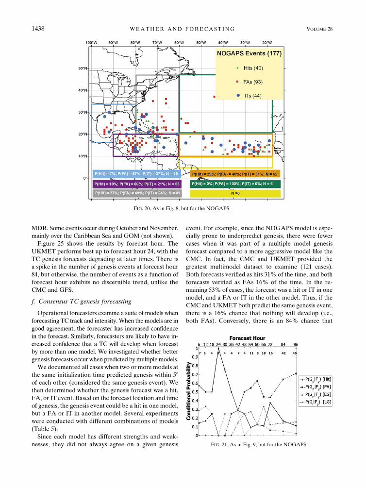
NOGAPS does not exhibit a distinct preferred re-

gion of genesis (Fig. 20), unlike the ECMWF and GFS

models, which clearly favor the MDR. Most of the

NOGAPS genesis events occur over the MDR, Ca-

ribbean Sea, and NW Atlantic, but very few occur

over the east-central Atlantic and equatorward of

108N.

NOGAPS exhibits seasonal preferences for TC gen-

esis. During June and July there are very few genesis

events. The majority of the genesis events occur during




August and September, coincident with the climato-

logical peak of TC activity. These events occur through-

out the basin. During October and November most

genesis events occur in the western Caribbean Sea and

GOM, consistent with the climatologically favored re-

gions of development for those months (not shown).

The small sample size of NOGAPS genesis events

as a function of forecast hour does not support any

definitive conclusions (Fig. 21). However, the model

appears more likely to develop a TC later in the forecast

period, and P(Gn jFy) increases with increasing forecast

hour, much like the CMC and GFS.

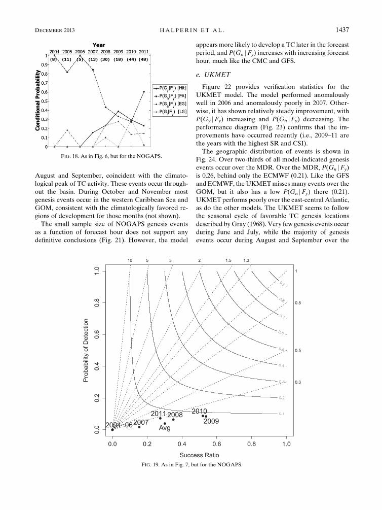
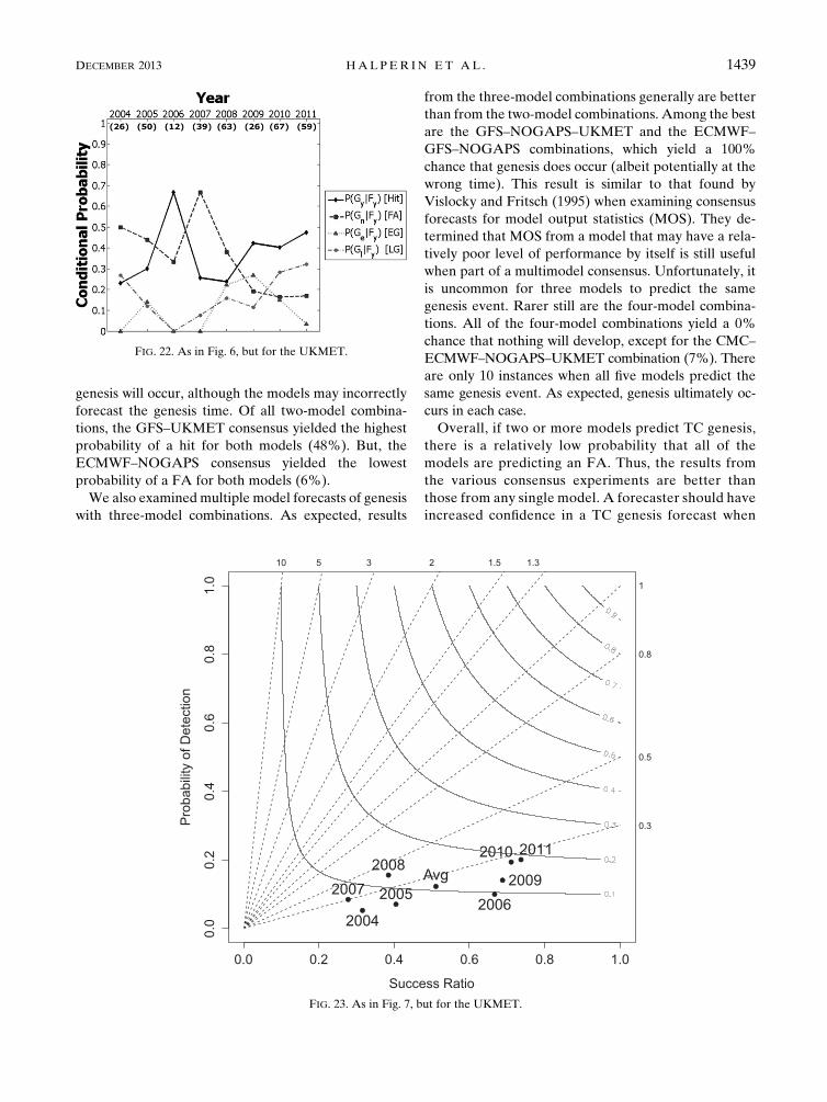
e. UKMET

Figure 22 provides verification statistics for the

UKMET model. The model performed anomalously

well in 2006 and anomalously poorly in 2007. Other-

wise, it has shown relatively steady improvement, with

P(Gy jFy) increasing and P(Gn jFy) decreasing. The

performance diagram (Fig. 23) confirms that the im-

provements have occurred recently (i.e., 2009–11 are

the years with the highest SR and CSI).

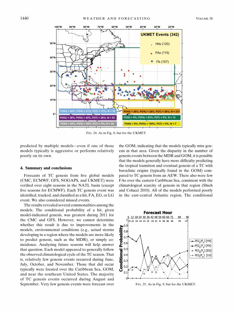
The geographic distribution of events is shown in

Fig. 24. Over two-thirds of all model-indicated genesis

events occur over the MDR. Over the MDR, P(Gn jFy)

is 0.26, behind only the ECMWF (0.21). Like the GFS

and ECMWF, theUKMETmisses many events over the

GOM, but it also has a low P(Gn jFy) there (0.21).

UKMETperforms poorly over the east-central Atlantic,

as do the other models. The UKMET seems to follow

the seasonal cycle of favorable TC genesis locations

described byGray (1968). Very few genesis events occur

during June and July, while the majority of genesis

events occur during August and September over the

FIG. 18. As in Fig. 6, but for the NOGAPS.



MDR. Some events occur during October and November,

mainly over the Caribbean Sea and GOM (not shown).

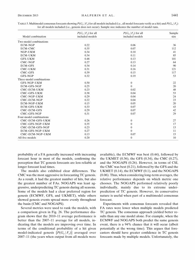
Figure 25 shows the results by forecast hour. The

UKMET performs best up to forecast hour 24, with the

TC genesis forecasts degrading at later times. There is

a spike in the number of genesis events at forecast hour

84, but otherwise, the number of events as a function of

forecast hour exhibits no discernible trend, unlike the

CMC and GFS.

f. Consensus TC genesis forecasting

Operational forecasters examine a suite of models when

forecasting TC track and intensity.When themodels are in

good agreement, the forecaster has increased confidence

in the forecast. Similarly, forecasters are likely to have in-

creased confidence that a TC will develop when forecast

by more than one model. We investigated whether better

genesis forecasts occur when predicted bymultiplemodels.

We documented all cases when two or more models at

the same initialization time predicted genesis within 58of each other (considered the same genesis event). We

then determined whether the genesis forecast was a hit,

FA, or IT event. Based on the forecast location and time

of genesis, the genesis event could be a hit in one model,

but a FA or IT in another model. Several experiments

were conducted with different combinations of models

(Table 5).

Since each model has different strengths and weak-

nesses, they did not always agree on a given genesis

event. For example, since the NOGAPS model is espe-

cially prone to underpredict genesis, there were fewer

cases when it was part of a multiple model genesis

forecast compared to a more aggressive model like the

CMC. In fact, the CMC and UKMET provided the

greatest multimodel dataset to examine (121 cases).

Both forecasts verified as hits 31% of the time, and both

forecasts verified as FAs 16% of the time. In the re-

maining 53% of cases, the forecast was a hit or IT in one

model, and a FA or IT in the other model. Thus, if the

CMC and UKMET both predict the same genesis event,

there is a 16% chance that nothing will develop (i.e.,

both FAs). Conversely, there is an 84% chance that




genesis will occur, although the models may incorrectly

forecast the genesis time. Of all two-model combina-

tions, the GFS–UKMET consensus yielded the highest

probability of a hit for both models (48%). But, the

ECMWF–NOGAPS consensus yielded the lowest

probability of a FA for both models (6%).

We also examined multiple model forecasts of genesis

with three-model combinations. As expected, results

from the three-model combinations generally are better

than from the two-model combinations. Among the best

are the GFS–NOGAPS–UKMET and the ECMWF–

GFS–NOGAPS combinations, which yield a 100%

chance that genesis does occur (albeit potentially at the

wrong time). This result is similar to that found by

Vislocky and Fritsch (1995) when examining consensus

forecasts for model output statistics (MOS). They de-

termined that MOS from a model that may have a rela-

tively poor level of performance by itself is still useful

when part of a multimodel consensus. Unfortunately, it

is uncommon for three models to predict the same

genesis event. Rarer still are the four-model combina-

tions. All of the four-model combinations yield a 0%

chance that nothing will develop, except for the CMC–

ECMWF–NOGAPS–UKMET combination (7%). There

are only 10 instances when all five models predict the

same genesis event. As expected, genesis ultimately oc-

curs in each case.

Overall, if two or more models predict TC genesis,

there is a relatively low probability that all of the

models are predicting an FA. Thus, the results from

the various consensus experiments are better than

those from any single model. A forecaster should have

increased confidence in a TC genesis forecast when

FIG. 22. As in Fig. 6, but for the UKMET.



predicted by multiple models—even if one of those

models typically is aggressive or performs relatively

poorly on its own.

4. Summary and conclusions

Forecasts of TC genesis from five global models

(CMC, ECMWF, GFS, NOGAPS, and UKMET) were

verified over eight seasons in the NATL basin (except

five seasons for ECMWF). Each TC genesis event was

identified, tracked, and classified as a hit, FA, EG, or LG

event. We also considered missed events.

The results revealed several commonalities among the

models. The conditional probability of a hit, given

model-indicated genesis, was greatest during 2011 for

the CMC and GFS. However, we cannot determine

whether this result is due to improvements in the

models, environmental conditions (e.g., actual storms

developing in a region where the models are more likely

to predict genesis, such as the MDR), or simply co-

incidence. Analyzing future seasons will help answer

that question. Each model appeared to generally follow

the observed climatological cycle of the TC season. That

is, relatively few genesis events occurred during June,

July, October, and November. Those that did occur

typically were located over the Caribbean Sea, GOM,

and near the southeast United States. The majority

of TC genesis events occurred during August and

September. Very few genesis events were forecast over

the GOM, indicating that the models typically miss gen-

esis in that area. Given the disparity in the number of

genesis events between theMDRandGOM, it is possible

that the models generally have more difficulty predicting

the tropical transition and eventual genesis of a TC with

baroclinic origins (typically found in the GOM) com-

pared to TC genesis from an AEW. There also were few

FAs over the eastern Caribbean Sea, consistent with the

climatological scarcity of genesis in that region (Shieh

and Colucci 2010). All of the models performed poorly

in the east-central Atlantic region. The conditional




probability of a FA generally increased with increasing

forecast hour in most of the models, confirming the

perception that TC genesis forecasts are less reliable at

longer forecast lead times.

The models also exhibited clear differences. The

CMCwas the most aggressive in forecasting TC genesis.

As a result, it had the greatest number of hits, but also

the greatest number of FAs. NOGAPS was least ag-

gressive, underpredicting TC genesis during all seasons.

Some of the models had a clear preferred region for

genesis (ECMWF, GFS, and UKMET), while others

showed genesis events spread more evenly throughout

the basin (CMC and NOGAPS).

Several metrics were used to rank the models, with

a comparison given in Fig. 26. The performance dia-

gram shows that the 2010–11 average performance is

better than the 2007–11 average for all models, in-

dicating that the models are improving over time. In

terms of the conditional probability of a hit given

model-indicated genesis [P(Gy jFy)] averaged over

2007–11 (the years when output from all models were

available), the ECMWF was best (0.44), followed by

the UKMET (0.36), the GFS (0.34), the CMC (0.27),

and the NOGAPS (0.26). However, in terms of CSI,

the CMC was best (0.21), followed by the GFS and the

UKMET (0.14), the ECMWF (0.1), and the NOGAPS

(0.06). Thus, when considering long-term averages, the

relative performance depends on which metric one

chooses. The NOGAPS performed relatively poorly

individually, mainly due to its extreme under-

prediction of TC genesis. However, its conservative

nature is useful when part of a multimodel consensus

forecast.

Experiments with consensus forecasts revealed that

FA rates were lower when multiple models predicted

TC genesis. The consensus approach yielded better re-

sults than any one model alone. For example, when the

ECMWF and NOGAPS both predict the same genesis

event, there is a 94% chance that it will occur (albeit

potentially at the wrong time). This argues that fore-

casters should have greater confidence in TC genesis

forecasts made by multiple models. Unfortunately, the

TABLE 5.Multimodel consensus forecasts showingP(Gy jFy) for all models included (i.e., all model forecasts verify as a hit) andP(Gn jFy)

for all models included (i.e., genesis does not occur). Sample size indicates the number of model runs.

Model combination

P(Gy jFy) for all

included models

P(Gn jFy) for all

included models

Sample

size

Two-model combinations

ECM–NGP 0.22 0.06 36

ECM–CMC 0.35 0.07 112

NGP–UKM 0.34 0.10 41

ECM–UKM 0.34 0.11 85

GFS–UKM 0.48 0.13 101

CMC–NGP 0.27 0.13 64

ECM–GFS 0.34 0.14 90

CMC–UKM 0.31 0.16 121

CMC–GFS 0.39 0.15 117

GFS–NGP 0.32 0.19 53

Three-model combinations

GFS–NGP–UKM 0.50 0 22

ECM–GFS–NGP 0.25 0 20

CMC–ECM–UKM 0.23 0.02 48

CMC–GFS–UKM 0.38 0.04 53

CMC–NGP–UKM 0.29 0.04 24

CMC–ECM–NGP 0.22 0.04 23

ECM–NGP–UKM 0.15 0.05 20

ECM–GFS–UKM 0.33 0.07 43

CMC–ECM–GFS 0.29 0.07 42

CMC–GFS–NGP 0.31 0.07 29

Four-model combinations

CMC–ECM–GFS–UKM 0.26 0 27

CMC–GFS–NGP–UKM 0.35 0 17

CMC–ECM–GFS–NGP 0.23 0 13

ECM–GFS–NGP–UKM 0.27 0 11

CMC–ECM–NGP–UKM 0.13 0.07 15

All five models 0.20 0 10


sample size of such consensus forecasts is relatively

small.

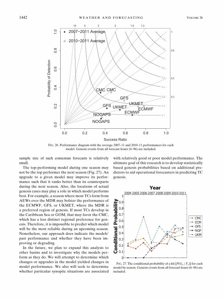
The top-performing model during one season may

not be the top performer the next season (Fig. 27). An

upgrade to a given model may improve its perfor-

mance such that it ranks better than its counterparts

during the next season. Also, the locations of actual

genesis cases may play a role in which model performs

best. For example, a season where most TCs form from

AEWs over the MDR may bolster the performance of

the ECMWF, GFS, or UKMET, where the MDR is

a preferred region of genesis. If most TCs develop in

the Caribbean Sea or GOM, that may favor the CMC,

which has a less distinct regional preference for gen-

esis. Therefore, it is impossible to predict which model

will be the most reliable during an upcoming season.

Nonetheless, our approach does indicate the models’

past performance and whether they have been im-

proving or degrading.

In the future, we plan to expand this analysis to

other basins and to investigate why the models per-

form as they do. We will attempt to determine which

changes or upgrades in the model yielded changes in

model performance. We also will seek to determine

whether particular synoptic situations are associated

with relatively good or poor model performance. The

ultimate goal of this research is to develop statistically

based genesis probabilities based on additional pre-

dictors to aid operational forecasters in predicting TC

genesis.

FIG. 26. Performance diagram with the average 2007–11 and 2010–11 performances for each

model. Genesis events from all forecast hours (6–96) are included.

FIG. 27. The conditional probability of a hit [P(Gy j Fy)] for each

model by season. Genesis events from all forecast hours (6–96) are

included.


Acknowledgments. The authors thank Ryan Truche-

lut, who provided some of the initial ideas for this re-

search. We are also indebted to Julian Heming of the

Met Office for providing some of the model output and

upgrade information that was necessary to carry out

this research. ECMWF output was obtained from the

TIGGE archive (ECMWF portal). We thank the

anonymous reviewers, as well as Chris Landsea and

Dave Zelinsky, who conducted the NHC internal re-

view. Thanks to Ron McTaggart-Cowan and Dave

Ryglicki for providing references for model upgrades.

The authors also benefited from discussions with Pat

Harr at NPS and Mike Fiorino at ESRL regarding this

research topic and from the suggestion by SimAberson at

HRD to display some of our results using the perfor-

mance diagrams. Finally, this research was supported by

NOAA/COMET Partner’s Project Z12-93225, NASA

GRIP Grant NNX09AC43G, and a Florida State Uni-

versity fellowship.

APPENDIX A

Selected Model Upgrades

a. CMC (B�elair et al. 2009; Charron et al. 2012)

Implemented 31 October 2006

d Horizontal grid spacing reduced from 100 to 33 kmd Number of vertical levels increased from 28 to 58d Time step reduced from 45 to 15mind Kuo transient shallow convection scheme added

(none previously)d Deep convection scheme changed from Kuo to

Kain–Fritsch

Implemented 22 June 2009

d Vertical coordinate changed from normalized s to

hybrid s pressured Number of vertical levels increased from 58 to 80d Model top raised from 10 to 0.1 hPa

b. ECMWF (2012)

d June 2007—replaced shortwave radiation schemewith

Rapid Radiative Transfer Modeld November 2007—updated convection schemed November 2007—updated vertical diffusion above the

boundary layerd June 2008—updated moist physics in the tangent

linear and adjointmodels used in the four-dimensional

variational data assimilation (4DVAR) schemed September 2008—used high-resolution SST from the

Met Office

d September 2008—introduced a simple representation

of the diurnal cycle of SSTd September 2009—introduced a new approach for

quality controlling conventional observationsd January 2010—horizontal resolution changed from

T799 (;25 km) to T1279 (;16 km)d November 2010—new cloud scheme implemented

c. GFS (Environmental Modeling Center 2012)

d May 2005—horizontal resolution changed from

T254L64 to 84 h and T170L42 to 180 h to T382L64 to

180 hd May 2007—changed to a hybrid s-pressure vertical

coordinated May 2007—unified the NCEP 3DVAR system under

the gridpoint statistical interpolation (GSI)d July 2010—horizontal resolution changed to T574L64

to 192 hd July 2010—made changes to the hurricane relocation

algorithmd July 2010—upgraded boundary layer schemed July 2010—new mass flux shallow convection scheme

addedd July 2010—updated deep convection scheme

d. NOGAPS (NRL 2012; COMET 2012)

d September 2004—changes made to the convective mo-

mentum transport within the Emanuel parameterizationd 2005—TC bogus scheme improvedd September 2009—model resolution increased from

T239L30 to T239L42d September 2009—switched from a 3DVAR data

assimilation system to the 4DVAR extension of the

Naval Research Laboratory Atmospheric Variational

Data Assimilation System (NAVDAS-AR)d September 2010—model resolution increased from

T239L42 to T319L42d 2010—vertical hybrid coordinate implemented

e. UKMET (J. Heming 2012, personalcommunication)

d October 2004—introduction of 4DVARd January 2005—model physics upgradedd December 2005—horizontal grid spacing decreased to

40 kmd December 2005—increase to 50 vertical levelsd December 2006—GPS radio occultation (GPSRO)

data introducedd May 2007—model physics upgradedd November 2008—model physics upgradedd November 2009—model physics and dynamics revised


d November 2009—increase to 70 vertical levelsd March 2010—horizontal grid spacing decreased to

25 kmd July 2010—new cloud scheme introducedd July 2011—hybrid data assimilation introduced

APPENDIX B

REFERENCES

B�elair, S., M. Roch, A.-M. Leduc, P. A. Vaillancourt, S. Laroche,

and J.Mailhot, 2009:Medium-range quantitative precipitation

forecasts from Canada’s new 33-km deterministic global op-

erational system. Wea. Forecasting, 24, 690–708.

Beven, J. L., 1999: The Boguscane—A serious problem with the

NCEP Medium Range Forecast model in the tropics. Pre-

prints, 23rd Conf. on Hurricanes and Tropical Meteorology,

Dallas, TX, Amer. Meteor. Soc., 845–848.

Braun, S. A., and Coauthors, 2013: NASA’s Genesis and Rapid

Intensification Processes (GRIP) field experiment. Bull.

Amer. Meteor. Soc., 94, 345–363.

Briegel, L. M., and W. M. Frank, 1997: Large-scale influences on

tropical cyclogenesis in the western North Pacific. Mon. Wea.

Rev., 125, 1397–1413.Camargo, S. J., K. A. Emanuel, and A. H. Sobel, 2007: Use of

a genesis potential index to diagnose ENSO effects on tropical

cyclone genesis. J. Climate, 20, 4819–4834.Chan, J. C. L., and R. H. F. Kwok, 1999: Tropical cyclone genesis in

a global numerical weather predictionmodel.Mon.Wea. Rev.,

127, 611–624.

Charney, J. G., and A. Eliassen, 1964: On the growth of the hur-

ricane depression. J. Atmos. Sci., 21, 68–75.

Charron, M., and Coauthors, 2012: The stratospheric extension of

the Canadian Global Deterministic Medium-Range Weather

Forecasting System and its impact on tropospheric forecasts.

Mon. Wea. Rev., 140, 1924–1944.

Cheung, K. W., and R. L. Elsberry, 2002: Tropical cyclone for-

mations over the western North Pacific in the Navy Opera-

tional Global Atmospheric Prediction System Forecasts.Wea.

Forecasting, 17, 800–820.

COMET, cited 2012: NOGAPS 4.0 introduction. UCAR COMET

Program. [Available online at http://www.meted.ucar.edu/

nwp/pcu2/nogaps/index.htm.]

Cot�e, J., J. G. Desmarais, S. Gravel, A. M�ethot, A. Patoine,

M. Roch, and A. Staniforth, 1998a: The operational CMC–

MRB Global Environmental Multiscale (GEM) model. Part

II: Results. Mon. Wea. Rev., 126, 1397–1418.——, S. Gravel, A. M�ethot, A. Patoine, M. Roch, and A. Staniforth,

1998b: The operational CMC–MRB Global Environmental

Multiscale (GEM) model. Part I: Design considerations and

formulation. Mon. Wea. Rev., 126, 1373–1395.

Craig, G. C., and S. L. Gray, 1996: CISK or WISHE as the mech-

anism for tropical cyclone intensification. J. Atmos. Sci., 53,

3528–3540.

Cullen, M. J. P., 1993: The Unified Forecast/Climate Model. Me-

teor. Mag., 122, 81–94.Dunkerton, T. J., M. T. Montgomery, and Z. Wang, 2008: Tropical

cyclogenesis in a tropical wave critical layer: Easterly waves.

Atmos. Chem. Phys., 8, 11 149–11 292.

ECMWF, cited 2012: ECMWFannual reports. [Available online at

http://www.ecmwf.int/publications/annual_report/.]

Elsberry, R. L., W. M. Clune, and P. A. Harr, 2009: Evaluation of

global model early track and formation prediction in the

western North Pacific. Asia-Pac. J. Atmos. Sci., 45, 357–374.——, M. S. Jordan, and F. Vitart, 2010: Predictability of tropical

cyclone events on intraseasonal timescales with the ECMWF

monthly forecast model. Asia-Pac. J. Atmos. Sci., 46, 135–

153.

——, ——, and ——, 2011: Evaluation of the ECMWF 32-day

ensemble predictions during 2009 season of western North

Pacific tropical cyclone events on intraseasonal timescales.

Asia-Pac. J. Atmos. Sci., 47, 305–318.

Emanuel, K. A., 1986: An air–sea interaction theory for tropical

cyclones. Part I: Steady-state maintenance. J. Atmos. Sci., 43,

585–605.

——, 1988: Themaximum intensity of hurricanes. J. Atmos. Sci., 45,

1143–1155.

——, andD. S.Nolan, 2004: Tropical cyclones and the global climate

system. Preprints, 26th Conf. on Hurricanes and Tropical Me-

teorology, Miami Beach, FL, Amer. Meteor. Soc., 10A.1.

[Available online at https://ams.confex.com/ams/pdfpapers/

75463.pdf.]

Enagonio, J., and M. T. Montgomery, 2001: Tropical cyclogenesis

via convectively forced vortex Rossby waves in a shallow

water primitive equation model. J. Atmos. Sci., 58, 685–706.

Environmental Modeling Center, cited 2012: GFS/GDAS changes

since 1991. [Available online at http://www.emc.ncep.noaa.

gov/gmb/STATS/html/model_changes.html.]

Frank,W.M., andG. S. Young, 2007: The interannual variability of

tropical cyclones. Mon. Wea. Rev., 135, 3587–3598.Goerss, J. S., 2000: Tropical cyclone track forecasts using an

ensemble of dynamical models. Mon. Wea. Rev., 128, 1187–

1193.

TABLE B1. Terms referenced in the text and their associated

acronyms and equations/symbols.

Name Acronym Equation/symbol

Hit event a

False alarm event FA b

Miss event c

Early genesis event EG e

Late genesis event LG f

Incorrect timing event IT e1 f

Conditional probability

of a hit

P(Gy jFy)a

a1 b1 e1 f


of a false alarm

P(Gn jFy)b

a1 b1 e1 f


of an early genesis event

P(Ge jFy)e

a1 b1 e1 f


of a late genesis event

P(Gl jFy)f

a1 b1 e1 f


of an incorrect timing event

P(Gt jFy)e1 f

a1 b1 e1 f

Probability of detection PODa

a1 c

Success rate SR 12b

a1b

Biasa1 b

a1 c

Critical success index CSIa

a1 b1 c


http://www.meted.ucar.edu/nwp/pcu2/nogaps/index.htm

http://www.meted.ucar.edu/nwp/pcu2/nogaps/index.htm

http://www.ecmwf.int/publications/annual_report/

https://ams.confex.com/ams/pdfpapers/75463.pdf


http://www.emc.ncep.noaa.gov/gmb/STATS/html/model_changes.html

http://www.emc.ncep.noaa.gov/gmb/STATS/html/model_changes.html

——, C. R. Sampson, and J. M. Gross, 2004: A history of western

North Pacific tropical cyclone track forecast skill. Wea. Fore-

casting, 19, 633–638.

Gray, W. M., 1968: Global view of the origin of tropical distur-

bances and storms. Mon. Wea. Rev., 96, 669–700.

Jarvinen, B. R., C. J. Neumann, and M. A. S. Davis, 1984: A tropical

cyclone data tape for the North Atlantic basin, 1886–1983: Con-

tents, limitations, and uses. NWS NHC Tech. Memo. 22, 24 pp.

Kanamitsu, M., 1989: Description of the NMC global data assimi-

lation and forecast system. Wea. Forecasting, 4, 335–342.

Marchok, T. P., 2002: How the NCEP tropical cyclone tracker

works. Preprints, 25th Conf. on Hurricanes and Tropical Mete-

orology, San Diego, CA, Amer. Meteo. Soc., P1.13. [Available

online at https://ams.confex.com/ams/25HURR/webprogram/

Paper37628.html.]

McAdie, C. J., C. W. Landsea, C. J. Neumann, J. E. David,

E. Blake, and G. R. Hammer, 2009: Tropical cyclones of the

North Atlantic Ocean, 1851–2006. Historical Climatology

Series 6-2, National Climatic Data Center–NHC, 238 pp.

McTaggart-Cowan, R., G. D. Deane, L. F. Bosart, C. A. Davis, and

T. J. Galarneau, 2008: Climatology of tropical cyclogenesis in

theNorthAtlantic (1948–2004).Mon.Wea.Rev., 136, 1284–1304.

Montgomery, M. T., and J. Enagonio, 1998: Tropical cyclogenesis via

convectively forced vortex Rossby waves in a three-dimensional

quasigeostrophic model. J. Atmos. Sci., 55, 3176–3207.

——, V. S. Nguyen, J. Persing, and R. K. Smith, 2009: Do tropical

cyclones intensify by WISHE? Quart. J. Roy. Meteor. Soc.,

135, 1697–1714.

——, and Coauthors, 2012: The Pre-Depression Investigation of

Cloud-Systems in the Tropics (PREDICT) experiment: Sci-

entific basis, new analysis tools, and some first results. Bull.

Amer. Meteor. Soc., 93, 153–172.

NHC, cited 2011: NHC track and intensity models. [Available

online at http://www.nhc.noaa.gov/modelsummary.shtml.]

NRL, cited 2012: MarineMeteorology Division history. [Available

online at http://www.nrlmry.navy.mil/MMD_History/text/

frame.htm.]

Pasch, R. J., P. A. Harr, L. A. Avila, J. G. Jiing, and G. Elliot, 2006:

An evaluation and comparison of predictions of tropical cy-

clogenesis by three global forecast models. Preprints, 27th

Conf. on Hurricanes and Tropical Meteorology, Monterey,

CA, Amer. Meteor. Soc., 14B.5. [Available online at https://

ams.confex.com/ams/pdfpapers/108725.pdf.]

——, E. S. Blake, J. G. Jiing, M. M. Mainelli, and D. P. Roberts,

2008: Performance of the GFS in predicting tropical cyclone

genesis during 2007. Preprints, 28th Conf. on Hurricanes and

Tropical Meteorology, Orlando, FL, Amer. Meteor. Soc.,

11A.7. [Available online at https://ams.confex.com/ams/

28Hurricanes/techprogram/paper_138218.htm.]

Rappaport, E. N., and Coauthors, 2009: Advances and challenges at

the National Hurricane Center. Wea. Forecasting, 24, 395–419.

Ritchie, E. A., and G. J. Holland, 1997: Scale interactions during

the formation of Typhoon Irving.Mon. Wea. Rev., 125, 1377–

1396.

Roebber, P. J., 2009: Visualizing multiple measures of forecast

quality. Wea. Forecasting, 24, 601–608.

Rogers, R., and Coauthors, 2006: The Intensity Forecasting Ex-

periment: A NOAA multiyear field program for improving

tropical cyclone intensity forecasts. Bull. Amer. Meteor. Soc.,

87, 1523–1537.

Rosmond, T. E., 1992: The design and testing of the Navy Opera-

tional Global Atmospheric Prediction System. Wea. Fore-

casting, 7, 262–272.

Sampson, C. R., andA. J. Schrader, 2000: TheAutomated Tropical

Cyclone Forecasting System (version 3.2).Bull. Amer.Meteor.

Soc., 81, 1231–1240.

——, J. L. Franklin, J. A. Knaff, and M. DeMaria, 2008: Experi-

ments with a simple tropical cyclone intensity consensus.Wea.

Forecasting, 23, 304–312.Shieh, O. H., and S. J. Colucci, 2010: Local minimum of tropical

cyclogenesis in the eastern Caribbean. Bull. Amer. Meteor.

Soc., 91, 185–196.Simpson, J., E. Ritchie, G. J. Holland, J. Halverson, and S. Stewart,

1997: Mesoscale interactions in tropical cyclone genesis.Mon.

Wea. Rev., 125, 2643–2661.

Tory, K. J., and W. M. Frank, 2010: Tropical cyclone formation.

Global Perspectives on Tropical Cyclones: From Science to

Mitigation, J. C. L. Chan and J. D. Kepert, Eds., World Sci-

entific, 55–91.

Tsai, H.-C., K.-C. Lu, R. L. Elsberry, M.-M. Lu, and C.-H. Sui, 2011:

Tropical cyclone–like vortices detection in the NCEP 16-day

ensemble system over the western North Pacific in 2008: Ap-

plication and forecast evaluation. Wea. Forecasting, 26, 77–93.Vislocky, R. L., and J. M. Fritsch, 1995: Improved model output

statistics forecasts through model consensus. Bull. Amer.

Meteor. Soc., 76, 1157–1164.

Walsh, K. J. E., M. Fiorino, C. W. Landsea, and K. L. McInnes,

2007: Objectively determined resolution-dependent threshold

criteria for the detection of tropical cyclones in climatemodels

and reanalyses. J. Climate, 20, 2307–2314.

Wilks, D. S., 2006: Statistical Methods in the Atmospheric Sciences.

2nd ed. Academic Press, 627 pp.


https://ams.confex.com/ams/25HURR/webprogram/Paper37628.html

https://ams.confex.com/ams/25HURR/webprogram/Paper37628.html

http://www.nhc.noaa.gov/modelsummary.shtml

http://www.nrlmry.navy.mil/MMD_History/text/frame.htm

http://www.nrlmry.navy.mil/MMD_History/text/frame.htm



https://ams.confex.com/ams/28Hurricanes/techprogram/paper_138218.htm

https://ams.confex.com/ams/28Hurricanes/techprogram/paper_138218.htm

An Evaluation of Tropical Cyclone Genesis Forecasts from...

Documents

Transcript of An Evaluation of Tropical Cyclone Genesis Forecasts from...