NASA/TP—2011–216466

An Estimate of the North Atlantic Basin Tropical Cyclone Activity for the 2011 Hurricane SeasonRobert M. WilsonMarshall Space Flight Center, Marshall Space Flight Center, Alabama

June 2011

National Aeronautics andSpace AdministrationIS20George C. Marshall Space Flight CenterMarshall Space Flight Center, Alabama35812

The NASA STI Program…in Profile

Since its founding, NASA has been dedicated to the advancement of aeronautics and space science. The NASA Scientific and Technical Information (STI) Program Office plays a key part in helping NASA maintain this important role.

The NASA STI Program Office is operated by Langley Research Center, the lead center for NASA’s scientific and technical information. The NASA STI Program Office provides access to the NASA STI Database, the largest collection of aeronautical and space science STI in the world. The Program Office is also NASA’s institutional mechanism for disseminating the results of its research and development activities. These results are published by NASA in the NASA STI Report Series, which includes the following report types:

• TECHNICAL PUBLICATION. Reports of completed research or a major significant phase of research that present the results of NASA programs and include extensive data or theoretical analysis. Includes compilations of significant scientific and technical data and information deemed to be of continuing reference value. NASA’s counterpart of peer-reviewed formal professional papers but has less stringent limitations on manuscript length and extent of graphic presentations.

• TECHNICAL MEMORANDUM. Scientific and technical findings that are preliminary or of specialized interest, e.g., quick release reports, working papers, and bibliographies that contain minimal annotation. Does not contain extensive analysis.

• CONTRACTOR REPORT. Scientific and technical findings by NASA-sponsored contractors and grantees.

• CONFERENCE PUBLICATION. Collected papers from scientific and technical conferences, symposia, seminars, or other meetings sponsored or cosponsored by NASA.

• SPECIAL PUBLICATION. Scientific, technical, or historical information from NASA programs, projects, and mission, often concerned with subjects having substantial public interest.

• TECHNICAL TRANSLATION. English-language translations of foreign

scientific and technical material pertinent to NASA’s mission.

Specialized services that complement the STI Program Office’s diverse offerings include creating custom thesauri, building customized databases, organizing and publishing research results…even providing videos.

For more information about the NASA STI Program Office, see the following:

• Access the NASA STI program home page at <http://www.sti.nasa.gov>

• E-mail your question via the Internet to <help@sti.nasa.gov>

• Fax your question to the NASA STI Help Desk at 443 –757–5803

• Phone the NASA STI Help Desk at 443 –757–5802

• Write to: NASA STI Help Desk NASA Center for AeroSpace Information 7115 Standard Drive Hanover, MD 21076–1320

i

NASA/TP—2011–216466

An Estimate of the North Atlantic Basin Tropical Cyclone Activity for the 2011 Hurricane SeasonRobert M. WilsonMarshall Space Flight Center, Marshall Space Flight Center, Alabama

June 2011

National Aeronautics andSpace Administration

Marshall Space Flight Center • MSFC, Alabama 35812

ii

Available from:

NASA Center for AeroSpace Information7115 Standard Drive

Hanover, MD 21076 –1320443 –757– 5802

This report is also available in electronic form at<https://www2.sti.nasa.gov/login/wt/>

iii

TABLE OF CONTENTS

1. INTRODUCTION ............................................................................................................. 1

2. RESULTS AND DISCUSSION ......................................................................................... 2

2.1 Statistical Aspects of the North Atlantic Basin Tropical Cyclones (1950–2010) ............ 2 2.2 The Effect of El Niño-Southern Oscillation Phase on Tropical Cyclone Activity .......... 10 2.3 The Effect of a Warming World on Tropical Cyclone Activity ...................................... 22 2.4 Statistical Aspects of the Onset Location of Tropical Cyclones .................................... 28 2.5 Statistical Aspects of the PWS, <PWS>, LP, and <LP> ............................................... 34 2.6 Statistical Aspects of the Differences (Yearly Value Minus the 10-yma Value) .............. 43 2.7 Estimating <AT>, <ONI>, <SOI>, and <NAO> for 2011 From Their Early Observed Monthly Values in 2011 ................................................................................. 51

3. SUMMARY ........................................................................................................................ 57

REFERENCES ....................................................................................................................... 60

iv

LIST OF FIGURES

1. Yearly and 10-yma seasonal frequencies of (a) NTC, (b) NH, (c) NMH, and (d) NUSLFH for 1950–2010 ................................................................................ 3

2. Yearly seasonal variation of (a) fd(NTC)10, (b) fd(NH)10, (c) fd(NMH)10, and (d) fd(NUSLFH)10 for 1950–2004 ....................................................................... 8

3. Yearly and 10-yma seasonal variations of (a) <ONI>, (b) <SOI>, (c) <NAO>, and (d) ENSO for 1950–2010 ..................................................................................... 11

4. El Niño (1950–2010): (a) Duration, (b) max ONI, (c) <<ONI>>, and (d) rp ............ 15

5. La Niña (1950–2010): (a) Duration, (b) max ONI, (c) <<ONI>>, and (d) rp ........... 16

6. Scatter plots against <ONI>10: (a) (NTC)10, (b) (NH)10, (c) (NMH)10, and (d) (NUSLFH)10 for various time intervals ......................................................... 17

7. Scatter plots against <SOI>10: (a) (NTC)10, (b) (NH)10, (c) (NMH)10, and (d) (NUSLFH)10 for various time intervals ......................................................... 18

8. Scatter plots against <NAO>10: (a) (NTC)10, (b) (NH)10, (c) (NMH)10, and (NUSLFH)10 for various time intervals ............................................................... 19

9. Yearly seasonal variation of (a) fd(<ONI>10), (b) fd(<SOI>10), and (c) fd(<NAO>10) for 1950–2004 .......................................................................... 21

10. Yearly and 10-yma seasonal variations of (a) <AT> and (b) <MLCO2> for 1950–2010 ............................................................................................................. 23

11. Yearly seasonal variation of (a) fd(<AT>10) and (b) fd(<MLCO2>10) for 1950–2004 ............................................................................................................. 24

12. Scatter plots against <AT>10: (a) (NTC)10, (b) (NH)10, (c) (NMH)10,

and (d) (NUSLFH)10 for various time intervals ......................................................... 27

13. Yearly and 10-yma seasonal variations of (a) <LAT> and (b) <LONG> for 1950–2010 ............................................................................................................. 29

14. Scatter plots against <ONI>10: (a) <LAT>10 and (b) <LONG>10 and <SOI>10: (c) <LAT>10 and (d) <LONG>10 for different time intervals .................................... 30

15. Scatter plots against <NAO>10: (a) <LAT>10 and (b) <LONG>10 and <AT>10: (c) <LAT>10 and (d) <LONG>10 ....................................................... 31

v

LIST OF FIGURES (Continued)

16. Yearly variation of (a) fd(<LAT>10) and (b) fd(<LONG>10) for 1950–2004 ............. 33

17. Scatter plots against <LAT>10: (a) (NTC)10, (b) (NH)10, (c) (NMH)10, and (d) (NUSLFH)10 for different time intervals ....................................................... 35

18. Scatter plots against <LONG>10: (a) (NTC)10, (b) (NH)10, (c) (NMH)10, and (d) (NUSLFH)10 for different time intervals ....................................................... 36

19. Yearly and 10-yma seasonal variations of (a) PWS, (b) <PWS>, (c) LP, and (d) <LP> for 1950–2010 ...................................................................................... 38

20. Scatter plots: (a) (LP)10 vs. (PWS)10; (b) <LP>10 vs. <PWS>10; (c) <PWS>10 vs. (PWS)10; and (d) <LP>10 vs. (LP)10 ...................................................................... 41

21. Scatter plots of (PWS)10, <PWS>10, (LP)10, and <LP>10 vs. left-most panels, <ONI>10; left-middle panels, <SOI>10; middle-right panels, <NAO>10; and right-most panels <AT>10 ................................................................................... 42

22. Yearly variation of (a) fd(PWS10), (b) fd(<PWS>10), (c) fd(LP10), and (d) fd(<LP>10) for 1950–2004 ............................................................................. 44

23. Yearly variation of (a) d(NTC), (b) d(NH), (c) d(NMH), and (d) d(NUSLFH) for 1950–2005 ............................................................................................................. 45

24. Yearly variation of (a) d(<AT>), (b) d(<ONI>), (c) d(<SOI>), and (d) d(<NAO>) for 1950–2005 .............................................................................. 48

25. Yearly variation of (a) d(<LAT>) and (b) d(<LONG>) for 1950–2005 ..................... 49

26. Yearly variation of (a) d(PWS), (b) d(<PWS>), (c) d(LP), and (d) d(<LP>) for 1950–2005 ............................................................................................................. 50

27. Comparison of 2011 monthly values against the 1995–2010 monthly mean and extremes of (a) Armagh Observatory surface air temperature and (b) the Oceanic Niño Index ................................................................................. 52

28. Comparison of 2011 monthly values against the 1995–2010 monthly mean and extremes of the Southern Oscillation Index ......................................................... 53

29. Comparison of 2011 monthly values against the 1995–2010 monthly mean and extremes of the North Atlantic Oscillation Index ................................................ 54

vi

LIST OF TABLES

1. Frequency distribution of NTC, NH, NMH, and NUSLFH for 1950–2010 .............. 5

2. Poisson probabilities for NTC, NH, NMH, and NUSLFH for selected time intervals: 1950–1994, 1995–2010, and 1950–2010 ....................................................... 6

3. Frequency distribution of first-difference 10-yma values for NTC, NH, NMH, and NUSLFH for selected time intervals: 1950–1989, 1990–2004, and combined ..... 9

4. Inferred statistical regressions between <ONI>, <SOI>, and <NAO> using 10-yma values (1955–2005) ......................................................................................... 12

5. Listing of El Niño and La Niña events based on ONI (ERSST.v3b) .......................... 13

6. Inferred statistical regressions between 10-yma values of tropical cyclones and 10-yma values of <ONI>, <SOI>, and <NAO> for selected time intervals ........ 20

7. Inferred statistical regressions between <ONI>, <SOI>, <NAO>, <AT>, and <MLCO2> for selected time intervals ................................................................. 25

8. Inferred regressions between 10-yma values of tropical cyclones and 10-yma values of <AT> for selected time intervals ................................................................. 28

9. Inferred statistical regressions between 10-yma values of <LAT> and <LONG> against <ONI>, <SOI>, <NAO>, and <AT> (1950–2005) ....................................... 32

10. Inferred statistical regressions between 10-yma values of tropical cyclones and 10-yma values of <LAT> and <LONG> for 1950–2005 ..................................... 37

11. Inferred statistical regressions between <AT>, <ONI>, <SOI>, and <NAO> against their running monthly means based on 1995–2010 ......................................... 55

vii

LIST OF ACRONYMS, SYMBOLS, AND ABBREVIATIONS

2-mma 2-month moving average

10-yma 10-year moving average

A April, August

AT monthly mean of Armagh temperature

<AT> yearly mean of Armagh temperature

<AT>10 10-yma of <AT>

B before

D December

Dur. duration

d difference

EN El Niño

ENSO El Niño-Southern Oscillation

ERSST.v3 extended reconstructed SST, version 3

F February

f frequency

fd first difference

J January, June, July

<LAT> yearly mean of latitudinal locations of tropical cyclones at onset

<LAT>10 10-yma of <LAT>

LN La Niña

<LONG> yearly mean of longitudinal locations of tropical cyclones at onset

LP lowest pressure (in mb) of a tropical cyclone in a single season

<LP> mean LP (in mb) of all tropical cyclone LPs in a season

(LP)10 10-yma of LP

viii

LIST OF ACRONYMS, SYMBOLS, AND ABBREVIATIONS (Continued)

<LP>10 10-yma of <LP>

<LONG>10 10-yma of <LONG>

M moderate

<MLCO2> yearly mean of Mauna Loa Carbon Dioxide

<MLCO2>10 10-yma of <MLCO2>

max ONI maximum value of monthly Oceanic Niño Index

N November

NAO monthly value of the North Atlantic Oscillation Index

<NAO> yearly mean of North Atlantic Oscillation Index

<NAO>10 10-yma of <NAO>

NH number of hurricanes

(NH)10 10-yma of NH

NMH number of major hurricanes

(NMH)10 10-yma of NMH

NOAA National Oceanic and Atmospheric Administration

NTC number of tropical cyclones

(NTC)10 10-yma of NTC

NUSLFH number of United States land-falling hurricanes

(NUSLFH)10 10-yma of NUSLFH

O October

ONI monthly value of the Oceanic Niño Index

<ONI> yearly mean of ONI

<<ONI>> average ONI value over the duration of the event

<ONI>10 10-yma of <ONI>

PWS peak wind speed (in kt) of the strongest tropical cyclone in a season

ix

LIST OF ACRONYMS, SYMBOLS, AND ABBREVIATIONS (Continued)

<PWS> mean PWS (in kt) of all tropical cyclone PWSs in a season

(PWS)10 10-yma of PWS

<PWS>10 10-yma of <PWS>

rp recurrence period (elapsed time between same ENSO phase starts)

S September, strong, South latitude

SOI monthly value of the Southern Oscillation Index

<SOI> yearly mean of Southern Oscillation Index

<SOI>10 10-yma of <SOI>

SST sea surface temperature

TP Technical Publication

U.S. United States

W weak, West longitude

x

NOMENCLATURE

cl confidence level

e base of the Naperian system of logarithms

f frequency

m mean

n number

P(r) Poisson probability

r number of events in Poisson distribution, coefficient of correlation

sd standard deviation

se standard error of estimate

t the t statistic for independent sample

x independent variable

y dependent variable

1

TECHNICAL PUBLICATION

AN ESTIMATE OF THE NORTH ATLANTIC BASIN TROPICAL CYCLONEACTIVITY FOR THE 2011 HURRICANE SEASON

1. INTRODUCTION

Since about 1995 (16 seasons), the yearly frequency of tropical cyclones in the North Atlantic Basin has been greater, on average, than during the earlier interval 1950–1994 (45 seasons).1–14 In particular, the mean yearly (seasonal) frequency of tropical cyclones is now about 54% greater than what occurred during the earlier interval, the mean yearly frequency of hurricanes is about 41% greater, the mean yearly frequency of major or intense hurricanes is about 63% greater, and the mean yearly frequency of land-falling hurricanes along the coastline of the United States (U.S.) is about 30% greater. How long this current interval of increased yearly frequencies will persist is unknown, possibly being related to whether the increased activity is due to a natural multidecadal-scale varia-tion, the result of ongoing climatic change (i.e., the warming of the Earth’s atmosphere and ocean temperatures), or a combination of both.15–38

During the 2010 hurricane season,39 19 tropical cyclones formed in the North Atlantic Basin, including 12 hurricanes and 5 major hurricanes (i.e., those of category 3 or higher on the Saffir-Simpson hurricane scale, which have a sustained peak wind speed (PWS) ≥96 kt, or ≥111 mph). Fortunately, no U.S. land-falling hurricanes occurred, with the year 2010 becoming the 5th year since 1995 and the 13th year since 1950 that had no tropical cyclones striking the U.S. coastline as hurricanes.

In this NASA Technical Publication (TP), estimates for the number of tropical cyclones (NTC), number of hurricanes (NH), number of major hurricanes (NMH), and number of U.S. land-falling hurricanes (NUSLFH) are given for the 2011 North Atlantic Basin hurricane season based on a variety of statistical techniques. It is anticipated that the 2011 hurricane season for the North Atlantic Basin likely will see a continuation of the current trend of above long-term mean fre-quencies of tropical cyclones that has been in vogue since 1995.40,41 Also examined are the effects of the El Niño-Southern Oscillation (ENSO) phase and climatic change (global warming) on tropical cyclones, the variation of the seasonal centroid location of tropical cyclone onsets, and the varia-tion of peak wind speed and lowest pressure of tropical cyclones. (The National Hurricane Center’s Atlantic Tracks File 1851–2009 and end of the season reports for 2010 provide the basis for this analysis. In particular, for this study, the number of storms, onset locations, peak wind speeds and lowest pressures were ascertained using wind speed threshold as the determining factor.)

2

2. RESULTS AND DISCUSSION

2.1 Statistical Aspects of the North Atlantic Basin Tropical Cyclones (1950–2010)

Figure 1 displays the yearly seasonal frequencies (the thin, jagged line) and 10-year moving averages (10-yma; the thick, smoothed line) of (a) NTC, (b) NH, (c) NMH, and (d) NUSLFH for the interval 1950–2010. The horizontal lines in each panel represent the long-term means. Also shown are the standard deviation (sd), range, and sum for each grouping of tropical cyclones. Thus, for the interval 1950–2010, on average, the yearly seasonal frequency of tropical cyclones in the North Atlantic Basin is about 10.9 storms per year, having an sd of 4.1 storms per year, a range of 4 to 28 storms per year, and a total of 667 storms. Prior to 1995, NTC averaged about 9.6 storms per year, having an sd of about 2.8 storms per year and range of 4 to 18 storms per year, with only the year 1969 having NTC ≥15 storms per year. However, from 1995 onward, NTC has averaged about 14.8 storms per year, having an sd of about 4.7 storms per year and range of 8 to 28 storms per year, with 9 years having NTC ≥15 storms per year, including the years 1995, 2000, 2001, 2003, 2004, 2005, 2007, 2008, and 2010. Based on the behavior of the 10-yma of NTC, it appears to have been relatively flat until the onset of the current anomalous active state. From about 1994/1995 onward, the 10-yma of NTC has exceeded its long-term average, perhaps, attaining a plateau of about 15.3 storms per year in the years 2003–2005.

Regarding NH and NMH, their long-term means are, respectively, about 6.3 and 2.7 storms per year, having sds of about 2.7 and 2 storms per year, ranges of 2 to 15 and zero to 8 storms per year, and totals of 386 and 166 storms since 1950. Like NTC, the average yearly frequencies of NH and NMH prior to 1995 were somewhat lower than are seen from 1995 onward. During the earlier interval, NH and NMH averaged, respectively, about 5.7 and 2.3 storms per year, having sds of about 2.2 and 1.9 storms per year and ranges of 2 to 12 and zero to 8 storms per year, whereas during the current interval, NH and NMH average, respectively, about 8.1 and 3.8 storms per year, having sds of about 3.3 and 1.8 storms per year and ranges of 3 to 15 and 1 to 7 storms per year. Prior to 1995, only the years 1950 and 1969 each had NH ≥10 storms per year, while from 1995 onward, the years 1995, 1998, 2005, and 2010 each had NH ≥10 storms per year.

Regarding NMH, the differences are less apparent when contrasting the number of storms above a specific threshold for the two intervals, although differences are readily apparent, especially, when one interprets the temporal variation in NMH as being due to the existence of two states of activity—more active and less active. For example, prior to 1995, only the years 1950, 1951, 1955, 1958, 1961, 1964, and 1969 each had NMH ≥5, with no years between 1970–1994 having NMH ≥5. From 1995 onward, the years 1995, 1996, 1999, 2004, 2005, 2008, and 2010 each had NMH ≥5.

Based on the behavior of the 10-yma of NH, it too appears to have been relatively flat until the onset of the current anomalous active state. However, from about 1994/1995 onward the 10-yma of NH has exceeded its long-term average, possibly, attaining a plateau of about 8 storms per year from the year 2000 onward. Based on the behavior of the 10-yma of NMH, unlike NTC and NH,

3

mean = 1.6 sd = 1.5range = 0–6

mean = 2.7 sd = 2.0range = 0–8

mean = 6.3 sd = 2.7range = 2–15

mean = 10.9 sd = 4.1range = 4–28

NUSL

FH

NUSLFH = 9510

5

1950 1960 1970 1980 1990 2000 2010Year

(d)

(c)

NMH

NMH = 16610

5

(b)

NH

NH = 386

10

15

5

(a)

NTC

1950–2010NTC = 667

10

15

20

25

30

5

Figure 1. Yearly and 10-yma seasonal frequencies of (a) NTC, (b) NH, (c) NMH, and (d) NUSLFH for 1950–2010.

as aforementioned, its behavior strongly suggests the occurrences of more and less active states. The first more active state occurred prior to about the year 1966, and the second (current) more active state began about the year 1995 and continues through the present. The less active state (29 years in length) spans the years of about 1966–1994. (As used here, the basis for the approximate division

4

between more and less active states is the timing of the occurrences when the 10-yma for NMH crossed the long-term mean.)

Regarding NUSLFH, its long-term mean is about 1.6 hurricanes striking the U.S. coastline each year, having an sd of 1.5 strikes per year, a range of zero to 6 strikes per year, and a total of 95 strikes since 1950. Only the years 1964, 1985, 2004, and 2005 had NUSLFH ≥4 strikes per year. Since 1950, no U.S. hurricane strikes have occurred in only 13 years, including the years 1951, 1962, 1973, 1978, 1981, 1982, 1990, 1994, 2000, 2001, 2006, 2009, and 2010, and there has never occurred three consecutive years of no-strikes along the U.S. coastline of a hurricane during this 61-year inter-val. Prior to 1995, NUSLFH averaged about 1.4 strikes per year, having an sd of 1.3 strikes per year and a range of zero to 6 strikes per year, while, from 1995 onward, NUSLFH has averaged about 1.9 strikes per year, having an sd of 2 strikes per year and a range of zero to 6 strikes per year.

Table 1 provides the yearly frequency distributions of NTC, NH, NMH, and NUSLFH in tabular form, separating the distributions into three groupings: 1950–1994 (the early interval), 1995–2010 (the current interval), and 1950–2010 (the combined interval). For comparison, table 2 is included, which gives the probabilities of occurrence for specific frequencies of tropical cyclones based on the Poisson distribution using the observed means for the various groupings of tropical cyclones. The Poisson distribution42 is useful for providing the probability of occurrence of the num-ber of events per unit of measurement (time), assuming they occur randomly. The formula for the Poisson distribution can be written as

P(r) = (e–mmr)/r! , (1)

where r is the number of events (tropical cyclones), P(r) is the probability of r events occurring per unit of measurement (time), m is the mean number of events per unit of measurement, and e is the base of the Naperian system of logarithms.

As an example, for the interval 1950–1994, the single frequency of highest probability of occurrence for NTC is r = 9, having P(r) = 0.1293 or about 12.9%. The central seven frequencies of greatest probability of occurrence for NTC are r = 9 ± 3, having a combined probability of occur-rence equal to 0.0736 + 0.1010 + 0.1212 + 0.1293 + 0.1241 + 0.1083 + 0.0866 = 0.7441 or about 74.4%. Hence, under the assumption that seasonal frequencies of tropical cyclones occur randomly, one estimates a 74.4% probability that any one season will have NTC = 9 ± 3, based on the statistics for the interval of 1950–1994. In actuality, 39 of the 45 seasons during the years 1950–1994 had r = 9 ± 3, inferring an accuracy of prediction of about 86.7%.

For the now occurring interval (1995–2010), the probabilities are higher. For example, the central seven frequencies of greatest probability of occurrence for NTC are r = 14 ± 3, having a com-bined P(r) of about 63.7%. Had one estimated the yearly frequency of NTC to be r = 14 ± 3 for the interval 1995–2010 (16 seasons), one would have correctly predicted the seasonal frequency about 68.8% of the time (i.e., 11 of 16 seasons had frequencies of occurrence of tropical cyclones within the range of r = 14 ± 3). For NH, the combined P(r) = 62.4% for r = 8 ± 2; for NMH, the combined P(r) = 79.3% for r = 3 ± 2; and for NUSLFH, the combined P(r) = 72.5% for r = 1 ± 1. For each group-ing of tropical cyclones, the probability of exceeding the upper limit of the central prediction interval

5

Table 1. Frequency distribution of NTC, NH, NMH, and NUSLFH for 1950–2010.

f1950–1994 1995–2010 Combined

NTC NH NMH NUSLFH NTC NH NMH NUSLFH NTC NH NMH NUSLFH 0 4 8 5 4 13 1 13 23 1 3 14 26 2 1 14 4 4 3 1 18 7 3 6 6 8 2 3 3 8 9 11 4 1 9 1 1 1 1 1 10 2 1 5 1 5 3 1 4 1 6 7 6 4 9 2 1 2 2 4 9 3 3 7 6 7 1 2 1 6 9 2 8 7 4 1 1 2 8 6 1 9 3 2 1 4 4 6

10 4 1 1 5 111 8 1 1 8 212 5 1 2 1 7 213 3 1 414 2 1 315 4 1 4 116 2 21718 1 119 2 2202122232425262728 1 1

n 431 257 105 65 236 129 61 30 667 386 166 95mean 9.6 5.7 2.3 1.4 14.8 8.1 3.8 1.9 10.9 6.3 2.7 1.6sd 2.8 2.2 1.9 1.3 4.7 3.3 1.8 2.0 4.1 2.7 2.0 1.5

during the current more active phase is 23.5% for NTC, 19.4% for NH, 19.4% for NMH, and 27.5% for NUSLFH.

The above analysis presumes that the seasonal frequency of tropical cyclones is randomly distributed. However, because it is now well established that the phase of the ENSO phenomenon affects seasonal frequencies of tropical cyclones in the North Atlantic Basin and that the recent warming of the Earth’s atmosphere and oceans has created conditions more conducive to increased

6

Table 2. Poisson probabilities for NTC, NH, NMH, and NUSLFH for selected time intervals: 1950–1994, 1995–2010, and 1950–2010.

TimeInterval r

P(r)

TimeInterval r

P(r)NTC NH NMH NUSLFH NTC NH NMH NUSLFH

(m = 9.6) (m = 5.7) (m = 2.3) (m = 1.4) (m = 14.8) (m = 8.1) (m = 3.8) (m = 1.9)1950–1994

0 0.0001 0.0033 0.1003 0.2466 1995–2010

0 0.0000 0.0003 0.0224 0.28421 0.0007 0.0191 0.2306 0.3452 1 0.0000 0.0025 0.0850 0.27002 0.0031 0.0544 0.2652 0.2417 2 0.0000 0.0100 0.1615 0.17103 0.0100 0.1033 0.2033 0.1128 3 0.0002 0.0269 0.2046 0.08124 0.0240 0.1472 0.1169 0.0395 4 0.0007 0.0544 0.1944 0.03095 0.0460 0.1678 0.0538 0.0111 5 0.0022 0.0882 0.1477 0.00986 0.0736 0.1594 0.0206 0.0026 6 0.0055 0.1191 0.0936 0.00277 0.1010 0.1298 0.0068 0.0005 7 0.0115 0.1378 0.0508 0.00068 0.1212 0.0925 0.0019 0.0001 8 0.0213 0.1395 0.0241 0.00019 0.1293 0.0586 0.0005 0.0000 9 0.0351 0.1256 0.0102 0.0000

10 0.1241 0.0334 0.0001 10 0.0519 0.1017 0.003911 0.1083 0.0173 0.0000 11 0.0698 0.0749 0.001312 0.0866 0.0082 12 0.0861 0.0505 0.000413 0.0640 0.0036 13 0.0981 0.0315 0.000114 0.0439 0.0015 14 0.1037 0.0182 0.000015 0.0281 0.0006 15 0.1023 0.009816 0.0168 0.0002 16 0.0946 0.005017 0.0095 0.0001 17 0.0824 0.002418 0.0051 0.0000 18 0.0677 0.001119 0.0026 19 0.0528 0.000520 0.0012 20 0.0390 0.000221 0.0006 21 0.0275 0.000122 0.0002 22 0.0185 0.000023 0.0001 23 0.011924 0.0000 24 0.0073

25 0.004326 0.002527 0.001428 0.000729 0.000430 0.000231 0.000132 0.0000

7

TimeInterval r

P(r)NTC NH NMH NUSLFH

(m = 10.9) (m = 6.3) (m = 2.7) (m = 1.6)1950–2010

0 0.0000 0.0018 0.0672 0.20191 0.0002 0.0116 0.1815 0.32302 0.0011 0.0364 0.2450 0.25843 0.0040 0.0765 0.2205 0.13784 0.0109 0.1205 0.1488 0.05515 0.0237 0.1519 0.0804 0.01766 0.0430 0.1595 0.0362 0.00477 0.0669 0.1435 0.0139 0.00118 0.0912 0.1130 0.0047 0.00029 0.1105 0.0791 0.0014 0.0000

10 0.1204 0.0498 0.000411 0.1193 0.0285 0.000112 0.1084 0.0150 0.000013 0.0909 0.007314 0.0708 0.003315 0.0514 0.001416 0.0350 0.000517 0.0225 0.000218 0.0136 0.000119 0.0078 0.000020 0.004321 0.002222 0.001123 0.000524 0.000225 0.000126 0.0000

tropical cyclone formation and strengthening, strictly speaking, the seasonal frequencies may not be strictly randomly distributed.43–69 An examination of the distribution of the year-to-year change in the 10-yma values might provide better insight (as related to local trending) and possibly lead to an improved seasonal frequency forecast.

Figure 2 shows the variation of the year-to-year change in the 10-yma values of (a) NTC, (b) NH, (c) NMH, and (d) NUSLFH. The year-to-year change in 10-yma values is called the first-difference (fd) value. To the eye, it appears that there has been a slow transition from negative fd values to more positive fd values, at least for NTC, NH, and NMH. Indeed, runs-testing70 confirms that all fd distributions appear to be nonrandomly distributed. For example, the distribution of

Table 2. Poisson probabilities for NTC, NH, NMH, and NUSLFH for selected time intervals: 1950–1994, 1995–2010, and 1950–2010 (Continued).

8

fd(N

USLF

H)10

0.5

0

–0.51950 1960 1970 1980 1990 2000 2010

Year

(d)

(c)

fd(N

MH) 10

0.5

–0.5

0

(b)

fd(N

H)10

0.5

–0.5

0

–0.5

(a)

fd(N

TC) 10

1950–2004

0.5

1

0 mean = 0.09 sd = 0.29range = –0.4 to 0.9

mean = 0.02 sd = 0.21range = –0.4 to 0.5

mean = 0 sd = 0.18range = –0.4 to 0.4

mean = –0.01 sd = 0.14range = –0.3 to 0.5

Figure 2. Yearly seasonal variation of (a) fd(NTC)10, (b) fd(NH)10, (c) fd(NMH)10, and (d) fd(NUSLFH)10 for 1950–2004.

fd(NTC)10 has 34 values ≥0 in 10 runs, implying that the normal deviate (z) for the sample equals –2.88, which by hypothesis testing suggests that the distribution probably is nonrandom. Likewise, those for fd(NH)10, fd(NMH)10, and fd(NUSLFH)10, respectively, have 34, 31, and 38 values ≥0 in 11, 9, and 9 runs, implying z = –2.36, –3.43, and –3.19, which by hypothesis testing also suggests that these distributions probably are nonrandom.

Table 3 gives the fd distributions of the 10-yma of NTC, NH, NMH, and NUSLFH for the time intervals 1950–1989, 1990–2004, and 1950–2004 (combined). Noticeable is the close affinity of fd values to be near zero for the early time interval and the combined time interval, while being more positively skewed during the current interval (except for NUSLFH). For 1950–1989, fd(NTC)10, fd(NH)10, fd(NMH)10, and fd(NUSLFH)10 have values equal to 0 ± 0.1, respectively, in 24, 28, 29, and 31 of 40 seasons and, for the combined time interval, equal to 0 ± 0.1, respectively, in 28, 32, 36,

9

Table 3. Frequency distribution of first-difference 10-yma values for NTC, NH, NMH, and NUSLFH for selected time intervals: 1950–1989, 1990–2004, and combined.

fd1950–1989 1990–2004 Combined

NTC NH NMH NUSLFH NTC NH NMH NUSLFH NTC NH NMH NUSLFH10.9 1 10.8 2 20.70.6 2 20.5 1 2 1 1 2 10.4 3 1 3 3 1 30.3 2 4 2 1 2 1 1 3 6 1 30.2 4 1 2 1 2 5 4 6 6 6 10.1 9 6 7 2 2 2 5 11 6 9 70.0 3 7 13 23 2 3 2 4 5 10 15 27

–0.1 12 15 9 6 1 3 2 12 16 12 8–0.2 4 2 4 5 2 4 2 4 7–0.3 3 4 4 1 1 3 5 4 1–0.4 2 1 1 2 1 1–0.5

n 40 40 40 40 15 15 15 15 55 55 55 55mean –0.02 –0.04 –0.06 –0.02 0.39 0.17 0.15 0.05 0.09 0.02 0 0sd 0.20 0.17 0.14 0.12 0.30 0.22 0.18 0.18 0.29 0.21 0.18 0.14

and 42 of 55 seasons. However, for the current time interval, fd(NTC)10, fd(NH)10, and fd(NMH)10 have values equal to 0 ± 0.1, respectively, in only 4, 4, and 7 of 15 seasons, while fd(NUSLFH)10 has a value equal to 0 ± 0.1 in 11 of 15 seasons.

Because 10-yma fd values change little from one year to the next, the 10-yma fd values might prove useful for forecasting the expected ‘usual’ seasonal frequency of tropical cyclones based on the last known 10-yma value (the local trend). For example, using the combined interval statistics, one determines that the expected usual seasonal frequency of tropical cyclones (NTC) for the 2011 hurricane season should be about 20 [15.3 ± 0.1] – 2(140) – 15 = 11 ± 2, where 15.3 is the last known 10-yma of NTC (in 2005), 140 is the sum of all NTC values between the years 2002 and 2010, and 15 is the NTC value for the year 2001. However, because the current interval has, thus far, always had fd ≥0 (averaging about 0.4), the seasonal frequency for NTC in 2011 could easily be as high as 19 ± 2. Similarly, for NH, NMH, and NUSLFH, one finds the expected usual frequencies to be about 5 ± 2, 2 ± 2, and 0 ± 2, respectively, with seasonal frequencies possibly being as high as 8 ± 2, 5 ± 2, and 1 ± 2, respectively, for the 2011 hurricane season.

Although not shown here, it is noteworthy to mention that the range of differences between the actual seasonal frequencies of tropical cyclones and same year 10-yma values for NTC (i.e., d(NTC) = NTC – (NTC)10) has almost always been 0 ± 5 for all years 1950–2005. Only the years

10

1969, 1983, 1995, and 2005 had d(NTC) more negatively valued than –5 or more positively valued than 5. For these years d(NTC), respectively, equaled 7.9, –5.1, 7.9, and 12.7. In 2006, NTC = 10, so, providing that (NTC)10 for 2006 is not a statistical outlier, it follows that (NTC)10 should be equal to about 10 ± 5 in 2006. A value of (NTC)10 = 15 in 2006 implies fd = –0.3 in 2005 and NTC = 5 in 2011, while a value <15 implies a more negative value of fd in 2005 and a lower NTC in 2011. (NTC has always been 4 or more since 1950.) The lowest possible value for (NTC)10 in 2006 is 14.75, since such a value yields fd = –0.55 in 2005 and NTC = 0 in 2011. However, because the expected value of NTC for 2011 is >10, this implies that (NTC)10 >15.25 in 2006 and that fd will be more positive in value than –0.3 in 2005. Hence, the year 2006 very probably will be another statistical outlier year, at least with respect to d(NTC), like the years 1969, 1983, 1995, and 2005. (An fd = 0.2 in 2005 implies (NTC)10 = 15.5 in 2006 and NTC = 15 in 2011. See section 2.6.)

2.2 The Effect of El Niño-Southern Oscillation Phase on Tropical Cyclone Activity

As previously noted, it is well known that the phase of the ENSO can greatly influence the seasonal frequencies of tropical cyclones in the North Atlantic Basin, with lower seasonal frequen-cies being experienced when El Niño (EN) is occurring and higher seasonal frequencies when La Niña (LN) is occurring. Figure 3 depicts the yearly means of (a) the Oceanic Niño Index (<ONI>), (b) the Southern Oscillation Index (<SOI>), and (c) the North Atlantic Oscillation (<NAO>) Index, where the thin, jagged lines refer to the yearly means and the thick, smoothed lines refer to the 10-yma values of the yearly means. In recent years, the ONI has become the de facto standard that the National Oceanic and Atmospheric Administration (NOAA) uses for identifying warm (EN) and cool (LN) anomalous sea surface temperature (SST) episodes. In particular, an EN is said to be occurring when the 2-month moving average (2-mma), also called the 3-mo running mean, in the Extended Reconstructed SST version 3b (ERSST.v3b) of SST anomalies in the Niño 3.4 region of the Pacific Ocean (an area located between 5º N.–5º S. latitude and 120º–170º W. longitude) exceeds the threshold of 0.5 ºC for five or more consecutive months (from the base period spanning the years 1971–2000). Likewise, an LN is said to be occurring when the 2-mma dips below the threshold of –5 ºC for five or more consecutive months. When conditions not indicative of either an EN or LN episode are present, ENSO is said to be in the neutral (N) state.

The SOI is calculated from the monthly seasonal fluctuations in the air pressure difference between Tahiti, French Polynesia, and Darwin, Australia (based on means and sds calculated over the interval 1933–1992, inclusive). Sustained negative values of the SOI often are associated with EN episodes, while sustained positive values of the SOI often are associated with LN episodes. Hence, there exists a strong negative (inverse) correlation between SOI and ONI.

The NAO is calculated from the monthly seasonal fluctuations in the air pressure difference between the subtropical (Azores or Lisbon) high and the subpolar (Greenland or Iceland) low. The positive phase of NAO reflects below normal pressure across the high latitudes of the North Atlan-tic Ocean and above normal pressure across the central North Atlantic Ocean, whereas the negative phase reflects the opposite pattern. Both phases are associated with basin-wide changes in the inten-sity and location of the North Atlantic jet stream and storm tracks. Hence, positive (direct) correla-tion exists between NAO and ONI and negative (inverse) correlation exists between NAO and SOI.

11

<NAO

>

–0.5

0.5

1

1.5

–1

0

–1.5

1950

Calen

dar M

onth

1960 1970 1980 1990 2000 2010

ENLegend:

LNN

ONI ≥ 0.5ONI ≤ –0.5–0.5 < ONI < 0.5

Year

(c)

(d)

<SOI

>

–5

5

10

15

–10

0

–15

(b)

<ONI

>

–0.5

0.5

1

1.5

–1

0

–1.5(a)

1950–2010

DNOSAJJMAMFJ

mean = –0.01 sd = 0.62range = –1.24 to 1.29

mean = 0.08 sd = 7.03range = –13.1 to 15.4

mean = – 0.03 sd = 0.37range = –1.15 to 0.8

Figure 3. Yearly and 10-yma seasonal variations of (a) <ONI>, (b) <SOI>, (c) <NAO>, and (d) ENSO for 1950–2010.

12

Table 4 gives the inferred regression equations (from lowest to highest r) between <ONI>, <SOI>, and <NAO>, based on using the 10-yma values spanning the years 1955–2005. While all correlations are inferred to be statistically important at confidence level (cl) ≥99.9%, the correlations between the 10-yma values of <ONI> and <SOI> and between <NAO> and <SOI> are stronger than the one between <NAO> and <ONI>, with the preferential correlations able to explain (r2, the coefficient of determination) about 85%, 58%, and 39%, respectively, of the amount of variance in the 10-yma parametric values. (Based on yearly values, <ONI> and <SOI> are of opposite sign in 58 of the 61 years, being of the same sign only in 1952, 1978, and 1984. For <ONI> and <NAO>, they have been of opposite sign in 30 of the 61 years, while for <SOI> and <NAO>, they have been of opposite sign in 32 of 61 years.)

Table 4. Inferred statistical regressions between <ONI>, <SOI>, and <NAO> using 10-yma values (1955–2005).

Parameters Regression Equation r r×r se cl(%)<NAO> vs. <ONI> y = 0.007 + 0.614x 0.624 0.389 0.128 >99.9<ONI> vs. <NAO> y = 0.003 + 0.634x 0.624 0.389 0.130 >99.9<SOI> vs. <NAO> y = –0.482 – 11.292x –0.761 0.579 1.568 >99.9<NAO> vs. <SOI> y = –0.017 – 0.051x –0.761 0.579 0.208 >99.9<ONI> vs. <SOI> y = –0.032 – 0.063x –0.923 0.852 0.065 >99.9<SOI> vs. <ONI> y = –0.532 – 13.468x –0.923 0.852 0.930 >99.9

Interestingly, in figures 3(a)–(c), the 10-yma values of <ONI>, <SOI>, and <NAO> are now all near zero in value, suggesting, perhaps, the end of the decades-long intervals of predominantly positive (<ONI> and <NAO>) and negative (<SOI>) 10-yma values that are readily apparent in the figure panels. Of particular interest is the 2010 yearly value of <NAO>, which is the most negative value (–1.15) ever seen in the past 61 years. Such a strong negative <NAO>, perhaps, is suggestive that the 10-yma value of <NAO> might become more negatively valued over time, as it was prior to about 1973 (the 10-yma value of <NAO> was negatively valued between 1950 and 1973, positively valued between 1974 and 1999, and negatively valued once again beginning in 2000). Perhaps, this is a strong indication that the 10-yma value of <ONI> might also become more predominantly nega-tively valued over time, as well, as it was prior to about 1980, while the 10-yma value of <SOI> might also become more predominantly positively valued over time, as it was prior to about 1978.

Figure 3(d) depicts the phase of the ENSO, based on the reported monthly values of ONI, where the filled monthly intervals (of at least 5 mo duration) represent EN events, the cross-hatched monthly intervals (of at least 5 mo duration) represent LN events, and the unfilled monthly intervals represent periods of N, when neither an EN nor LN episode is occurring. In the years 1950–2010 (732 mo), there have been 182 mo classified EN, 201 mo classified LN, and 349 mo classified N. For the current interval (from 1995, 192 mo), there have been 53 mo classified EN, 51 mo classified LN, and 88 mo classified N.

Table 5 lists the start, peak, and end dates for EN and LN events since 1950 using ONI as the descriptor of the ENSO phase, and it also gives the duration (in months), max ONI, average

13

Table 5. Listing of El Niño and La Niña events based on ONI (ERSST.v3b).

Start Peak EndDur (mo) max ONI <<ONI>>

Event Type Strength

B01-1950 01-1950(?) 03 1951 >15 –1.7(?) - LN S08 1951 10 1951 12 1951 5 0.8 0.70 EN W04 1954 11 1955a 01 1957 34 –2.0 -0.98 LN S04 1957 01 1958 06 1958 15 1.7 0.99 EN S09 1962 11 1962* 01 1963 5 –0.7 –0.62 LN W07 1963 11 1963* 01 1964 7 1.0 0.86 EN M04 1964 10 1964* 01 1965 10 –1.2 –0.93 LN M06 1965 11 1965 04 1966 11 1.6 1.12 EN S12 1967 02 1968 04 1968 5 –0.9 –0.72 LN W11 1968 01 1969* 06 1969 8 1.0 0.79 EN M09 1969 11 1969 01 1970 5 0.8 0.66 EN W07 1970 01 1971*b 01 1972 19 –1.3 –0.91 LN M05 1972 12 1972 03 1973 11 2.1 1.32 EN S05 1973 12 1973c 05 1976 37 –2.1 –1.11 LN S09 1976 11 1976 02 1977 6 0.8 0.63 EN W 09 1977 11 1977a 01 1978 5 0.7 0.64 EN W05 1982 12 1982* 06 1983 14 2.3 1.39 EN S10 1984 12 1984 09 1985 12 –1.1 –0.71 LN M08 1986 08 1987*d 02 1988 19 1.6 1.11 EN S05 1988 11 1988* 05 1989 13 –1.9 –1.29 LN S05 1991 01 1992e 07 1992 15 1.8 1.13 EN S05 1994 12 1994 03 1995 11 1.3 0.83 EN M09 1995 11 1995f 03 1996 7 –0.7 –0.63 LN W05 1997 11 1997* 05 1998 13 2.5 1.74 EN S07 1998 12 1999* 06 2000 24 –1.6 –1.03 LN S10 2000 12 2000 02 2001 5 –0.7 –0.58 LN W05 2002 11 2002 03 2003 11 1.5 1.03 EN S06 2004 09 2004 02 2005 9 0.9 0.72 EN W08 2006 11 2006* 01 2007 6 1.1 0.83 EN M09 2007 01 2008* 05 2008 9 –1.4 –1.04 LN M06 2009 12 2009 04 2010 11 1.8 1.15 EN S07 2010 10 2010a – >7 –1.4? – LN M?

Averages: EN 10.1 1.4 0.98 LN 15.0@ –1.3@ –0.88@

Note: Bbefore ?uncertain *the month shown and the following month athe month shown and the two following months bmultiple peaks: –0.9 in September and November in 1970, –1.3 in January and February 1971, and –1 in November 1971 cmultiple peaks: –2.1 in December 1973, –1.1 in April 1974, –0.9 in November 1974, and –1.7 in November and December 1975 dmultiple peaks: 1.3 in February 1987, and 1.6 in August and September 1987 emultiple peaks: 1 in July 1991 and 1.8 in January 1992 fthe month shown and the following 3 mo @excludes before 01 1950 and 07 2010 events

14

ONI (<<ONI>>; i.e., the average ONI value over the duration of the event), and the strength of the anomaly, where W means weak ( 0.5 ºC ≤ ONI ≤ 0.9 ºC for EN episodes and –0.5 ºC ≤ ONI ≤ –0.9 ºC for LN episodes), M means moderate (1 ºC ≤ ONI ≤ 1.4 ºC for EN episodes and –1 ºC ≤ ONI ≤ –1.4 ºC for LN episodes), and S means strong (ONI ≥ 1.5 ºC for EN episodes and ONI ≤ –1.5 ºC for LN episodes). From the table, one notes that there have been 32 anomalous ENSO events since 1950, including 18 EN and 14 LN (one still ongoing). The strongest EN episode occurred May 1997 to May 1998, having max ONI = 2.5 ºC (November/December 1997), and the strongest LN episode occurred May 1973 to May 1976, having max ONI = –2.1. EN events average about 10 mo in length (range 5 to 19 mo), with the longest duration EN event having occurred August 1986 to February 1988 (19 mo), while LN events average about 15 mo in length (range 5 to 37 mo), with the longest duration LN event having occurred May 1973 to May 1976 (37 mo).

Figures 4 and 5 display the variations of (a) duration, (b) max ONI, (c) <<ONI>>, and (d) recurrence period (rp; i.e., the elapsed time between anomaly starts), respectively, for EN and LN events. In figures 4 and 5, W events are depicted as filled circles, M events are depicted as filled squares, and S events are depicted as filled triangles. For EN, there have been 5 W, 4 M, and 9 S events. Weak EN events average about 6 mo in duration (range 5 to 9 mo), 0.8 ºC in max ONI (range 0.7 to 0.9 ºC), and 0.67 ºC in <<ONI>> (range 0.63 to 0.72 ºC); moderate EN events average about 8 mo in duration (range 6 to 11 mo), 1.1 ºC in max ONI (range 1 to 1.3 ºC), and 0.83 ºC in <<ONI>> (range 0.79 to 0.86 ºC); and strong EN events average about 13 mo in duration (range 11 to 19 mo), 1.9 ºC in max ONI (range 1.6 to 2.5 ºC), and 1.22 ºC in <<ONI>> (range 0.99 to 1.74 ºC). Since EN events tend to recur about once every 40–41 mo, on average (range 10 to 75 mo), and the start of the last known EN event (a strong event) was June 2009, one does not anticipate the start of another EN event until 2012 or later, inferring that the 2011 hurricane season likely will be one when the ENSO phase will be either LN (a LN event presently continues in early 2011) or N. (From fig. 4(d), one finds that 8 of 8 strong EN events had an rp ≥25 mo, averaging about 49.4 mo and ranging between 25 and 75 mo, with 7 of 8 having an rp ≥36 mo, thereby, strongly suggesting that the start of the next EN event, indeed, will not occur until the summer of 2012 or later.)

For LN, there have been 4 W, 5 M, and 5 S events, although coverage for the first (an S event) and last (current, an M event)) events are incomplete (based on the published monthly record of ONI). For LN events with complete coverage (12 events), the weak LN events average about 5–6 mo in duration (range 5 to 7 mo), –0.8 ºC in max ONI (range 0.7 to 0.8 ºC), and 0.60 ºC in <<ONI>> (range 0.58 to 0.72 ºC); moderate LN events average about 12–13 mo in duration (range 10–19 mo), –1.3 ºC in max ONI (range –1.1 to –1.4 ºC), and –0.90 ºC in <<ONI>> (range –0.71 to –1.04 ºC); and strong LN events average about 27 mo in duration (range 13–37 mo), –1.9 ºC in max ONI (range –1.6 to –2.1 ºC), and –1.10 ºC in <<ONI>> (range 0.98 to –1.29 ºC). Presently, a moderate LN continues, having begun in July 2010 and having peaked in October–December 2010 (max ONI = –1.4 ºC). The question arises as to what is its expected duration? Since moderate LN events average about 12–13 mo in duration, one anticipates that the current moderate LN will linger at least through spring and possibly early summer 2011.71 Therefore, it seems very likely that the 2011 hurricane sea-son will be one having an ENSO phase classified either as LN or N, inferring that the frequencies of tropical cyclones in the North Atlantic Basin likely will be near to above post-1995 averages. (Based on the average rp for LN events, one does not anticipate the start of another LN event until 2013 or later.)

15

mean = 40.5 mo sd = 18.7 morange = 10–75 morp

(mo)

75

25

0

50

50 10 15 20Event Number

El Niño Events (1950–2010)

(d)

mean = 0.98 °C sd = 0.30 °Crange = 0.63–1.74 °C

<<ON

I>> (°

C)

2.0

1.0

0.5

1.5

(c)

mean = 10.1 mo sd = 4.1 morange = 5–19 mo

Dura

tion

(mo)

20

10

5

15

(a)

mean = 1.41 °C sd = 0.56 °Crange = 0.7–2.5 °C

max

ONI

(°C)

2.0

2.5

1.0

0.5

1.5

(b)

Figure 4. El Niño (1950–2010): (a) Duration, (b) max ONI, (c) <<ONI>>, and (d) rp.

16

mean = 56.3 mo sd = 36.9 morange = 19–137 mo

rp (m

o)

100

150

50

mean = –0.88 °C sd = 0.23 °Crange = –0.58 to –1.29 °C

–1.5

–1

–0.5

50 10 15Event Number

La Niña Events (1950–2010)

(d)

<<ON

I>> (°

C)

(c)

* excludes events 1 and 14

–1.5

–2.0

–2.5

–1

–0.5(b)

Dura

tion

(mo)

max

ONI

(°C)

mean* = 15 mo sd* = 11.2 morange = 5–37 mo

mean* = –1.3 °C sd* = 0.5 °Crange = –0.7 to –2.1 °C

* excludes events 1 and 14?

?

?

15

20

25

30

35

40

10

5(a)

Figure 5. La Niña (1950–2010): (a) Duration, (b) max ONI, (c) <<ONI>>, and (d) rp.

17

Figure 6 shows the scatter plots of 10-yma values of NTC ((NTC)10) versus 10-yma values of <ONI> (<ONI>10) for (a) the intervals 1950–1989, 1990–2005, and 1950–2005, (b) 10-yma val-ues of NH ((NH)10) versus <ONI>10 for the same intervals, (c) 10-yma values of NMH ((NMH)10) versus <ONI>10 for the same intervals, and (d) 10-yma values of NUSLFH ((NUSLFH)10) versus <ONI>10 for the same intervals. Included in each panel is the inferred coefficient of correlation r. Likewise, figures 7 and 8 show similar scatter plots against <SOI>10 and <NAO>10, respectively. In all plots, for the earlier interval (1950–1989) and the combined interval (1950–2005), the inferred correlations appear relatively weak. However, for the current interval (1990–2005), the inferred cor-relations appear relatively strong. This suggests that, at least for the current interval, the frequency of tropical cyclones in the North Atlantic Basin is more tightly coupled with the indices than was true in the earlier interval. (Table 6 gives the inferred regressions for each of the scatter plots.)

(NUS

LFH)

10

–5 0 5 50–5<ONI>10 <ONI>10 <ONI>10(d)

–5 0 5

r = –0.72 r = 0.175

r = –0.38

(NMH

) 10

(c)

r = –0.88 r = 05

r = –0.23

(NH)

10

(b)

r = –0.87 r = 0.1510

0

0

5

r = –0.39

(NTC

) 10

(a)

r = –0.89 r = 0.22

12

16

8

r = –0.55

1955–1989 1990–2005 1955–2005

Figure 6. Scatter plots against <ONI>10: (a) (NTC)10, (b) (NH)10, (c) (NMH)10, and (d) (NUSLFH)10 for various time intervals.

18

(NUS

LFH)

10

–5 0 5 50–5<SOI>10 <SOI>10 <SOI>10(d)

–5 0 5

r = 0.83 r = 0.185

r = 0.10

(NMH

) 10

(c)

r = 0.94 r = 0.085

r = 0.52

(NH)

10

(b)

r = 0.93 r = 0.1510

0

0

5

r = 0.61

(NTC

) 10

(a)

r = 0.97 r = –0.04

12

16

8

r = 0.62

1955–1989 1990–2005 1955–2005

Figure 7. Scatter plots against <SOI>10: (a) (NTC)10, (b) (NH)10, (c) (NMH)10, and (d) (NUSLFH)10 for various time intervals.

Figure 9 displays the observed fd values of the 10-yma values of (a) <ONI>, (b) <SOI>, and (c) <NAO>. As was previously found for fd(NTC)10, fd(NH)10, fd(NMH)10, and fd(NUSLFH)10, the values of fd(<SOI>)10 and fd(<NAO>)10 also appear to be nonrandomly distributed (hav-ing z = –2.25 and –3.33, respectively). However, the values of fd(<ONI>)10, in contrast, appear to be distributed randomly (having z = –0.54). For fd(<ONI>)10, 12 of 15 fd values fall within the range 0 ± 0.05 during the current interval (1990–2004) and 34 of 50 fd values fall within the range of 0 ± 0.05 for the combined interval (1955–2004); for fd(<SOI>)10, 10 of 15 fd values fall within the range 0 ± 0.50 for the current interval and 30 of 55 fd values fall within the range 0 ± 0.50 for the com-bined interval; and for fd(<NAO>)10, 14 of 15 fd values fall within the range 0 ± 0.05 during the cur-rent interval and 45 of 50 fd values fall within the range 0 ± 0.05 for the combined interval. Hence, on

19

(NUS

LFH)

10

–0.5 0 0.5 0.50–0.5<NAO>10 <NAO>10 <NAO>10(d)

–0.5 0 0.5

r = –0.81 r = –0.275

r = –0.19

(NMH

) 10

(c)

r = –0.97 r = –0.545

r = –0.80

(NH)

10

(b)

r = –0.96 r = –0.2710

0

0

5

r = –0.85

(NTC

) 10

(a)

r = –0.96 r = –0.01

12

16

8

r = –0.16

1955–1989 1990–2005 1955–2005

Figure 8. Scatter plots against <NAO>10: (a) (NTC)10, (b) (NH)10, (c) (NMH)10, and (NUSLFH)10 for various time intervals.

the basis of the usual behavior during the current interval, one anticipates that the 10-yma values of <ONI>, <SOI>, and <NAO> for 2006, respectively, will be equal to about 0.04 ± 0.05, 0.13 ± 0.50, and –0.12 ± 0.05, thereby, implying that <ONI>, <SOI>, and <NAO> for 2011, respectively, will be about –2.56 ± 1, –1.5 ± 10, and 1.18 ± 1, these values presupposing that the fd values for 2005 will fall within the aforementioned stated ranges.

While the 2011 anticipated values for <SOI> (= –11.5 to 8.5) and <NAO> (= 0.18 to 2.18) are generally within the range of past seasonal values, the one for <ONI> (= –3.56 to –1.56) clearly is not. Over the past 61 years, <ONI> has never dipped below –1.24 (1955) and its projected yearly value based on the usual expected 10-yma value for 2006 plainly is lower than any previously seen. Therefore, the indication is that, if the 2011 yearly projection of <ONI> is true, then the year 2011

20

Table 6. Inferred statistical regressions between 10-yma values of tropical cyclones and 10-yma values of <ONI>, <SOI>, and <NAO> for selected time intervals.

Time Interval Parameters Regression Equation r r×r se cl(%)1950–1989 NTC vs. ONI y = 9.459 – 1.696x –0.549 0.301 0.365 >99.9

NH vs. ONI y = 5.575 – 1.112x –0.392 0.154 0.367 >98NMH vs. ONI y = 2.148 – 1.130x –0.228 0.052 0.684 <90NUSLFH vs. ONI y = 1.525 + 0.745x 0.377 0.142 0.260 >95

1990–2005 NTC vs. ONI y = 15.451 – 17.302x –0.893 0.798 0.959 >99.9NH vs. ONI y =8.247 -7.904x –0.872 0.760 0.490 >99.9NMH vs. ONI y =4.027 -6.486x –0.877 0.768 0.394 >99.9NUSLFH vs. ONI y =2.107 -2.790x 0.718 0.515 0.298 >99.8

1950–2005 NTC vs. ONI y = 10.510 – 2.579x 0.224 0.050 1.858 <90NH vs. ONI y = 6.051 + 0.830x 0.154 0.024 0.886 <90NMH vs. ONI y = 2.457 + 0.001x 0.000 0.000 0.812 <90NUSLFH vs. ONI y = 1.535 + 0.334x 0.165 0.027 0.332 <90

1950–1989 NTC vs. SOI y = 9.632 + 0.139x 0.616 0.379 0.420 >99.9NH vs. ONI y = 5.747 + 0.147x 0.605 0.366 0.455 >99.9NMH vs. SOI y = 2.363 + 0.196x 0.522 0.273 0.742 >99.9NUSLFH vs. SOI y = 1.561 + 0.015x 0.098 0.010 0.346 <90

1990–2005 NTC vs. SOI y = 15.323 + 1.157x 0.966 0.934 0.549 >99.9NH vs. ONI y = 8.167 + 0.519x 0.926 0.857 0.376 >99.9NMH vs. SOI y = 3.969 + 0.429x 0.938 0.888 0.280 >99.9NUSLFH vs. SOI y = 2.116 + 0.200x 0.831 0.690 0.241 >99.9

1950–2005 NTC vs. SOI y = 10.525 – 0.028x –0.038 0.001 1.816 <90NH vs. ONI y = 6.158 + 0.055x 0.153 0.024 0.874 <90NMH vs. SOI y = 1.759 + 0.067x 0.076 0.006 2.139 <90NUSLFH vs. SOI y = 1.605 + 0.028x 0.184 0.034 0.361 <90

1950–1989 NTC vs. NAO y = 9.543 – 0.448x –0.162 0.026 0.431 <90NH vs. ONI y = 5.582 – 2.162x –0.855 0.730 0.203 >99.9NMH vs. NAO y = 2.120 – 3.538x –0.802 0.643 0.421 >99.9NUSLFH vs. NAO y = 1.474 – 0.338x –0.192 0.037 0.276 <90

1990–2005 NTC vs. NAO y = 14.086 – 14.012x –0.956 0.915 0.624 >99.9NH vs. ONI y =7.645 -6.618x –0.965 0.931 0.264 >99.9NMH vs. NAO y =3.535 -5.448x –0.973 0.947 0.188 >99.9NUSLFH vs. NAO y =1.898 -2.367x –0.805 0.648 0.252 >99.9

1950–2005 NTC vs. NAO y = 10.541 – 0.160x –0.014 0.000 1.907 <90NH vs. ONI y = 6.081 – 1.467x –0.267 0.071 0.862 >90NMH vs. NAO y = 2.493 – 2.682x –0.539 0.291 0.681 >99.9NUSLFH vs. NAO y = 1.547 – 0.564x –0.274 0.075 0.322 >90

21

mean = 0 °C sd = 0.06 °Crange = –0.11 to 0.15 °C

mean = –0.02 °C sd = 0.70 °Crange = –1.69 to 1.37 °C

mean = 0 °C sd = 0.03 °Crange = –0.10 to 0.08 °C

fd(<

NAO>

10)

fd(<

SOI> 10

)fd

(<ON

I> 10)

0.10

0.05

0

–0.05

–0.101950 1960 1970 1980 1990 2000 2010

Year

1950–2004

(c)

0

–0.5

0.5

1

1.5

2

–1

–1.5

–2(b)

0.10

0.05

0

–0.05

0.15

–0.10

(a)

Figure 9. Yearly seasonal variation of (a) fd(<ONI>10), (b) fd(<SOI>10), and (c) fd(<NAO>10) for 1950–2004.

22

will see a strong resurgence of LN activity and subsequently a significant increase in the frequency of tropical cyclones in the North Atlantic Basin; otherwise, the year 2011 will be a statistical outlier with respect to <ONI>, based on the usual behavior of the fd of the 10-yma values of <ONI>.

As an example, using the inferred regressions of (NTC)10, (NH)10, (NMH)10, and (NUSLFH)10 versus <NAO>10 (given in table 6) for the current interval (1990–2005), one estimates the 2006 values of (NTC)10, (NH)10, (NMH)10, and (NUSLFH)10, respectively, to be about 16.19 ± 0.62, 8.64 ± 0.26, 4.35 ± 0.19, and 2.25 ± 0.25 (i.e., the ±1 se prediction interval), based on using <NAO>10 = –0.15, where the <NAO>10 value for 2006 is computed from the known <NAO>10 value for 2005 (= –0.12) plus the expected fd value for 2005 (= –0.03, based on the average fd value found for the current interval). It follows then that (NTC)10 = 16.19 ± 0.62 implies NTC = 29 ± 12 for 2011, where ±12 is the range deduced from ±20 se (from the inferred regression fit given in table 6). Similarly, (NH)10 = 8.64 ± 0.26 implies NH = 22 ± 5 for 2011; (NMH)10 = 4.35 ± 0.19 implies NMH = 15 ± 4 for 2011; and (NUSLFH)10 = 2.25 ± 0.25 implies NUSLFH = 7 ± 5 for 2011. Presuming the validity of the inferred fits and the accuracy of the selected fd value (–0.03) for 2005, clearly, one anticipates that the 2011 hurricane season potentially could be considerably above average in activity, possibly even being a record-setting season. It should be noted, however, that a value of <NAO> higher than 1.18 in 2011 implies a more positive value than –0.12 for <NAO>10 in 2006, while a value lower than 1.18 implies a more negative value for <NAO>10 in 2006. Since <NAO> has never been higher than 0.80 in the past 61 years, it seems more likely that the 2006 value of <NAO>10 will be more negatively val-ued than the 2005 <NAO>10 value of –0.12 and that the number of tropical cyclones during the 2011 season will be greater than the current interval averages, unless, of course, the 2011 season proves to be a statistical outlier.

Similar findings are also found using <SOI>10 instead of <NAO>10. For example, using <SOI>10 = 0.43 for 2006 (equal to its 2005 value, 0.13, plus the expected fd, 0.30, based on the aver-age fd during the current interval), one estimates the 2006 values of (NTC)10, (NH)10, (NMH)10, and (NUSLFH)10, respectively, to be about 15.82 ± 0.55, 8.39 ± 0.38, 4.15 ± 0.28, and 2.20 ± 0.24. It follows then that the 2011 values for NTC, NH, NMH, and NUSLFH, respectively, should be about 21 ± 11, 17 ± 8, 11 ± 6, and 6 ± 5. Together, the expected values of the ENSO indices appear to suggest that the 2011 hurricane season for the North Atlantic Basin likely will be near to above average in activity.

2.3 The Effect of a Warming World on Tropical Cyclone Activity

In addition to the ENSO affecting the yearly frequency of tropical cyclones in the North Atlantic Basin, in recent years it has become apparent that the increasing warming of surface air and ocean temperatures, indicative of climatic change, creates conditions conducive for an increased frequency and strengthening of tropical cyclones. Surface air temperatures at Armagh Observatory (Northern Ireland) have been shown to serve as a useful proxy for global surface air temperatures and for monitoring the trend of the warming of the Earth.50 The Armagh Observatory temperature record extends from 1844 to the present.

Figure 10 displays the yearly variation of the means of (a) Armagh surface air tempera-ture (<AT> in ºC) and (b) Mauna Loa CO2 determinations (<MLCO2>, in ppm) for the interval 1950–2010. As in figures 1 and 3, the thin, jagged line plots the yearly means and the thick, smoothed

23

mean = 9.46 °C sd = 0.52 °Crange = 8.35 to 10.59 °C

<MLC

O2> (

ppm

)

300

350

400

1950 1960 1970 1980 1990 2000 2010Year(b)

<AT>

(°C)

1950–2010

8

8.5

9

9.5

10

10.5

11

(a)

Figure 10. Yearly and 10-yma seasonal variations of (a) <AT> and (b) <MLCO2> for 1950–2010.

line the 10-yma values. Because <MLCO2> (fig. 3(b)) has shown continuous (and generally accel-erating) year-to-year change, only the yearly means are plotted (for clarity). For the interval 1950–2010, <AT> has averaged 9.46 ºC (shown as the thin, horizontal line), having an sd of 0.52 ºC and a range of 8.35 to 10.59 ºC. The lowest <AT> occurred in 1979 and the highest in 2007. For the earlier interval 1950–1994, <AT> averaged 9.30 ºC, having an sd of 0.39 ºC and a range of 8.35 to 10.20 ºC, with the warmest year occurring in 1959. During this interval, <AT> exceeded 10 ºC only twice: 1959 (10.20 ºC) and 1989 (10.07 ºC). For the current interval 1995–2010, <AT> has averaged 9.97 ºC, having an sd of 0.47 ºC and a range of 8.74 to 10.59 ºC, where the lowest <AT> occurred in 2010 and the highest in 2007. During this interval, <AT> has exceeded 10 ºC in 10 of the 16 years, although the past 3 years have each had <AT> less than 10 ºC.

Interestingly, in figure 10(a) is the dip in 10-yma values of <AT> between about 1960 and 1990, reminiscent of the decline in 10-yma values, in particular, of NMH (fig. 1(c)). Such behavior is suggestive that the low activity interval (about 1966–1994), perhaps, might be low simply because surface air temperatures (and ocean temperatures) during the interval were slightly lower than either before about 1966 or after about 1994.8 During the interval 1966–1994, <AT> averaged just 9.26 ºC, as compared to 9.31 ºC during the preceding interval of 1950–1965 and 9.97 ºC after 1994.

Figure 10(b) shows that the yearly atmospheric concentration of CO2 as measured at Mauna Loa, Hawaii, has increased every year, without exception (1958–2010), from about 316 ppm in 1958

24

to 390 ppm in 2010, an increase of about 23% in 53 years and an increase of about 39% from pre-industrial levels (estimated to have been about 280 ppm). Carbon dioxide is the major greenhouse gas that affects the Earth’s surface air temperature, although others such as methane (CH4) and nitrous oxide (N2O) also contribute, but to a lesser extent.72

Figure 11 displays the fd of the 10-yma values of (a) <AT> (fd(<AT>10)) and (b) <MLCO2> (fd(<MLCO2>10)). Runs-testing clearly shows that fd(<AT>10) is distributed nonrandomly (z = 11.01), although year-to-year changes tend to be concentrated near 0 ± 0.05 ºC. Only the years 1957, 1963, 1964, 1980, and 2005 had fd(<AT>10) values of –0.06 ºC or cooler, while only the years 1983, 1984, 1989, 1990, 1991, 1992, 1997, 1998, 2000, and 2001 had fd(<AT>10) values of 0.06 ºC or warmer. Hence, 40 of 55 years (73%) had fd(<AT>10) = 0 ± 0.05 ºC. For fd(<MLCO2>10), it is increasing almost continuously, with the value in 2004 being 1.98 ppm.

mean = 0.01 °C sd = 0.05 °Crange = –0.08 to 0.13 °C

fd(<

MLCO

2>10

)

2

1.5

1

0.5

1950 1960 1970 1980 1990 2000 2010Year(b)

fd(<

AT> 10

)

–0.10

–0.05

0

0

0.05

0.10

0.15

(a)

Figure 11. Yearly seasonal variation of (a) fd(<AT>10) and (b) fd(<MLCO2>10) for 1950–2004.

Table 7 gives the inferred regression equations (from lowest to highest r) between <ONI>, <SOI>, <NAO>, and <MLCO2> against <AT> based on using the 10-yma values spanning the years 1950–2005. For the earlier interval 1950–1989, the only correlation inferred to be statistically important (cl ≥ 95%) is the one between <SOI> and <AT>. For the current interval 1990–2005, all correlations are inferred to be statistically very important (cl ≥ 99%), and for the combined interval

25

Table 7. Inferred statistical regressions between <ONI>, <SOI>, <NAO>, <AT>, and <MLCO2> for selected time intervals.

Time Intervals Parameters Regression Equation r r×r se cl(%)1950–1989 <ONI> vs. <AT>* 0.560 – 0.067x –0.059 0.004 0.141 <90

<AT> vs. <ONI>* 9.254 – 0.053x –0.059 0.004 0.271 <90<NAO> vs. <AT>* 1.855 – 0.203x –0.162 0.026 0.157 <90<AT> vs. <NAO>* 9.254 – 0.129x –0.162 0.026 0.278 <90<SOI> vs. <AT> –52.034 + 5.641x 0.321 0.103 2.200 >95<AT> vs. <SOI> 9.273 + 0.018x 0.321 0.103 0.115 >95

<AT> vs. <MLCO2>* 8.036 + 0.003x 0.380 0.144 1.288 <90

1990–2005 <ONI> vs. <AT> 4.171 – 0.407x –0.842 0.709 0.053 >99.9<AT> vs. <ONI> 10.125 – 1.739x –0.842 0.709 0.106 >99.9<SOI> vs. <AT> –71.999 + 7.081x 0.904 0.818 0.765 >99.9<AT> vs. <SOI> 10.110 + 0.116x 0.904 0.818 0.147 >99.9<NAO> vs. <AT> 6.037 – 0.603x –0.942 0.888 0.049 >99.9<AT> vs. <NAO> 9.994 – 1.473x –0.942 0.888 0.066 >99.9

<AT> vs. <MLCO2> 0.66374 + 0.02511x 0.948 0.899 0.045 >99.9

1950–2005 <NAO> vs. <AT> & –0.483 + 0.053x 0.104 0.011 0.162 <90<AT> vs. <NAO>& 9.439 + 0.205x 0.104 0.011 0.326 <90<SOI> vs. <AT> 14.265 – 1.557x –0.195 0.038 2.407 <90<AT> vs. <SOI> 9.430 – 0.024x –0.195 0.038 0.310 <90

<ONI> vs. <AT>& –1.973 + 0.210x 0.408 0.167 0.151 >99.5<AT> vs. <ONI>& 9.4331 + 0.7935x 0.408 0.167 0.295 >99.5

<AT> vs. <MLCO2>#

3.34780 + 0.01762x 0.905 0.820 0.102 >99.9

Note: *interval for <ONI> and <NAO> vs. <AT> is 1955–1989; and the interval for <AT> vs. <MLCO2> is 1964–1989 &interval for <ONI> and <NAO> vs. <AT> is 1955–2005 #interval is 1964–2005

1950–2005, only the correlations between <ONI> and <AT> and between <AT> and <MLCO2> are inferred to be statistically very important. Hence, at least for the current interval, it appears that given a reliable estimate of <AT>10 for the year 2006, one can crudely estimate the 10-yma values of <ONI>, <SOI>, and <NAO> for 2006 and, subsequently, estimate their 2011 yearly values, as well, or visa versa. It should be noted, however, that, although <AT>10 and <MLCO2>10 appear to be highly correlated, especially during the current interval, <AT>10 actually decreased during the last 3 years of the interval, from 10.13 to 10.02 ºC, while <MLCO2>10 continued to rise throughout the interval 1990–2005. Obviously, the CO2 level alone does not entirely explain the complete variation in <AT> from year to year—cloud cover, cosmic rays, volcanic aerosols, and solar irradiance also are known contributors.73–105 (Interestingly, the years 2007–2009, which factor in the 10-yma of <AT>, are associated with the current sunspot cycle’s prolonged sunspot minimum, the longest in more than 100 years. This may indicate a reduction in the total solar irradiance and less solar heating of the Earth’s atmosphere and oceans during this solar minimum, as compared to other recent solar minima.)

26

As an exercise, figure 11(b) suggests that the fd(<MLCO2>)10 for 2005 should be about 1.9–2 ppm, inferring that <MLCO2>10 for 2006 should be about 379.54 + (1.9–2) or about 381.5 ppm and that the <MLCO2> for 2011 should be about 390 ppm (or higher). Presuming <MLCO2>10 = 381.5 ppm for 2006, one can use the inferred preferential regression for the current interval between <AT>10 and <MLCO2>10 to estimate the expected value of <AT>10 for 2006, which turns out to be about 10.24 ± 0.05º. Such a value, however, has two serious drawbacks. First, it implies that fd<AT>10 would be 0.22 ± 0.05 ºC for 2005, a value larger than any ever seen in the inter-val 1950–2004. Recall that 40 of 55 previous years (only 7 of 15 years in the current interval) had fds that always lay within the range of 0 ± 0.05 ºC, with the largest positive fd increase to date being only 0.13 ºC in 1984. Second, it implies that <AT> = 15.15 ± 1 ºC for 2011, a value considerably higher than the highest <AT> to date, which is 10.59 ºC in 2007. Hence, it appears that the lack of directly correlated behavior between <MLCO2> and <AT> that has been underway since 2007 seems likely to continue in 2011. (Instead, if one uses the inferred correlation between <AT>10 and <MLCO2>10 from the combined interval, one finds <AT>10 = 10.07 ± 0.10 ºC for 2006 and <AT> = 11.75 ± 2 ºC for 2011, values that are much more reasonable.)

Another approach for estimating <AT>10 for 2006 might be to simply use <AT>10 = 10.02 ± 0.05 ºC, where 10.02 ºC is the last known value of <AT>10 for 2005 and the ±0.05 ºC is the expected usual fd<AT>10 value (i.e., fd<AT>10 = 0 ± 0.05 C, which has been seen previously in 40 of 55 years). Presuming this to be true, one estimates <AT> for 2011 to be about 10.75 ± 1 ºC (up from 8.74 ºC that was seen in 2010), which if true, likewise suggests that 2011 possibly will be a year of near-record warmth, possibly higher than the previous warmest year in 2007 that measured 10.59 ºC. Applying 10.02 ºC in the inferred regression equations (table 7) for the current interval, one estimates <ONI>10 = 0.09 ± 0.053 ºC for 2006 and <ONI> = –1.56 ± 1.06 ºC for 2011, this latter value indica-tive of LN conditions. Similarly, for <SOI>10 and <NAO>10 for 2006, one estimates values of about –1.05 ± 0.765 and –0.005 ± 0.049, respectively, and about –25.1 ± 15.3 and 3.48 ± 0.98, respectively, for 2011. While the 2011 inferred value for <ONI> (and possibly <SOI>) appears somewhat reason-able, the one for <NAO> is not. This may be an indication that the inferred preferentially correlated behavior noted during the current interval between <ONI>, <SOI>, and <NAO> against <AT> might merely be a statistical fluke. Otherwise, the year 2011 will be a very strange year indeed.

Figure 12 depicts the scatter plots of (NTC)10, (NH)10, (NMH)10, and (NUSLFH)10 against <AT>10 for the earlier interval (left column), the current interval (middle column), and the com-bined interval (right column). The inferred coefficient of regression r is given in each panel. Plainly, one infers very strong associations between the 10-yma frequencies of tropical cyclones and surface air temperature as measured at the Armagh Observatory, especially during the current interval (since 1990).

Table 8 gives the inferred regressions of (NTC)10, (NH)10, (NMH)10, and (NUSLFH)10 against <AT>10. All correlations are inferred to be statistically very important for all time intervals (except the one between 10-yma values of NTC against 10-yma values of <AT> for the interval 1950–1989, which is only of marginal statistical significance). Using <AT>10 = 10.02 ºC for 2006 in the current interval inferred regressions, one estimates 10-yma values for NTC, NH, NMH, and NUSLFH for 2006 to be, respectively, 14.26 ± 0.56, 7.74 ± 0.11, 3.59 ± 0.22, and 1.94 ± 0.21. These values indicate only slight or no decrease as compared to their 2005 10-yma values for NH, NMH, and NUSLFH

27

(NUS

LFH)

10

9 9.5 10<AT>10(d)

5r = 0.70

9 9.5 10<AT>10

r = 0.87

9 9.5 10<AT>10

r = 0.83

(NMH

) 10

(c)

5r = 0.70 r = 0.97 r = 0.64

(NH)

10

(b)

10

0

0

5

r = 0.50 r = 0.99 r = 0.84

(NTC

) 10

1950–1989 1990–2005 1950–2005

(a)

12

16

8

r = 0.29 r = 0.97 r = 0.90

Figure 12. Scatter plots against <AT>10: (a) (NTC)10, (b) (NH)10, (c) (NMH)10,

and (d) (NUSLFH)10 for various time intervals.

(respectively, 7.8, 3.7, and 1.9), but an unrealistic decrease for NTC (from 15.3). While the inferred fd values for NH, NMH, and NUSLFH are well within the range of past values, the inferred fd for (NTC)10 is well outside-low the range of past values (i.e., –1.04 ± 0.56 as compared to the range of 0 ± 0.3, a range that has been true for 44 of the past 55 years, with 8 of the 11 outliers occurring dur-ing the current interval; the largest positive fd for (NTC)10 that has been seen thus far is 0.9 in 1999 and the largest negative fd is –0.4 in 1954 and 1974). From these inferred 10-yma values (based on <AT>10 = 10.02 ºC), one estimates NTC = 0–11, NH = 2–6, NMH = 0–4, and NUSLFH = 1–5 for 2011. (Presuming the veracity of the current interval fit between (NTC)10 and <AT>10, to obtain the average NTC deduced for the current interval, one requires <AT>10 warmer than 10.07 ºC in 2006, which implies <AT> = 11.75 ºC or higher in 2011, a temperature more than 1.16 ºC warmer than the highest temperature ever recorded at Armagh Observatory, 10.59 ºC in 2007.)

28

Table 8. Inferred regressions between 10-yma values of tropical cyclones and 10-yma values of <AT> for selected time intervals.

Time Interval Parameters Regression Equation r r×r se cl(%)1950-1989 NTC vs. AT y = –0.995 + 1.150x 0.289 0.084 0.503 >90

NH vs. AT y = –14.061 + 2.140x 0.499 0.249 0.478 >99.9NMH vs. AT y = –40.306 + 4.605x 0.698 0.487 0.629 >99.9NUSLFH vs. AT y = –15.668 + 1.857x 0.702 0.493 0.259 >99.9

1990-2005 NTC vs. AT y = –76.962 + 9.104x 0.971 0.943 0.563 >99.9NH vs. AT y = –35.601 + 4.325x 0.986 0.971 0.114 >99.9NMH vs. AT y = –31.299 + 3.482x 0.972 0.946 0.221 >99.9NUSLFH vs. AT y = –14.518 + 1.643x 0.873 0.763 0.213 >99.9

1950-2005 NTC vs. AT y = -39.524 + 5.303x 0.896 0.803 0.781 >99.9NH vs. AT y = –16.719 + 2.421x 0.838 0.703 0.459 >99.9NMH vs. AT y = –14.637 + 1.824x 0.636 0.405 0.684 >99.9NUSLFH vs. AT y = –7.780 + 0.993x 0.829 0.687 0.198 >99.9

2.3 Statistical Aspects of the Onset Location of Tropical Cyclones

Figure 13 depicts the yearly seasonal variation of the mean location (i.e., centroid) of tropi-cal cyclones onsets for the interval 1950–2010, in terms of (a) latitude (<LAT>) and (b) longitude (<LONG>). The yearly mean latitude and longitude of tropical cyclone onsets is simply the average latitude and longitude of all tropical cyclones in a single season at the time they first attained a sus-tained PWS ≥34 kt, or 39 mph. As an example, for the year 1983, there were four tropical cyclones that occurred during the hurricane season. These four storms first attained a sustained PWS ≥34 kt, respectively, at latitudes of 27.2º, 27.4º, 31.6º, and 28º N. and longitudes of 91.1º, 76.3º, 63.3º, and 73º W., thereby, yielding the centroid of <LAT> = 28.6º N. and <LONG> = 75.9º W. for the 1983 season. For the 2010 hurricane season, <LAT> and <LONG> for the 19 tropical cyclones at the time they first attained a sustained PWS ≥34 kt are 16.6º N. and 58.8º W., respectively. As before, the thin, jagged line is the yearly mean and the thick, smoothed line is the 10-yma value. The horizontal lines represent the long-term means. Hence, for the interval 1950–2010, the long-term seasonal mean <LAT> = 22.2º N., having sd = 3.4º and range equal to 16.2º–32.2º N., and the long-term seasonal mean <LONG> = 64.2º W., having sd = 6.2º and range equal to 51.8–79.4º W.

In the 1950s, the 10-yma centroid of latitude for tropical cyclones was below the long-term mean, rising above the mean in the mid 1960s. It continued above the long-term mean latitude until the late 1980s when it again fell below the long-term mean latitude. The 10-yma values of <LAT> have remained below the long-term mean since the late 1980s, with all individual years after 1986 having <LAT> below the long-term mean, except for the years 1991, 1992, 1997 and 2002, these years being associated with EN events. The most northerly extent of <LAT> occurred in 1972 (32.2º N.), again a year associated with an EN event, and the least northerly extent of <LAT> occurred in 1996 (16.2º N.), a year following an LN event.

29

mean = 64.2° W. sd = 6.2°range = 51.8–79.4° W.

<LON

G> (°

W.)

85

50

55

60

65

70

75

80

1950 1960 1970 1980 1990 2000 2010Year(b)

mean = 22.2° W. sd = 3.4°range = 16.2–32.2° N.

<LAT

> (°N

.)

15

20

25

30

35

(a)

Figure 13. Yearly and 10-yma seasonal variations of (a) <LAT> and (b) <LONG> for 1950–2010.

Similarly, the 10-yma centroid of longitude for tropical cyclones, while being more westerly (closer to the U.S. coastline) in the 1950s and again in the late 1960s through the mid 1980s, appears to be progressively moving more easterly (away from the U.S. coastline) over time, in conjunction with a prominent multidecadal variation. The most westerly extent of <LONG> occurred in 1956 (79.4º W.), a year following an LN event, and the most easterly extent of <LONG> occurred in 2009 (51.8º W.), a year associated with an EN event.

Together, the behavior of the 10-yma values of <LAT> and <LONG> appears to be related to basin-wide changes on multidecadal timescales, possibly related to changes in the 10-yma values of the ENSO indices and/or global temperature. Hence, seasonal changes in the centroid pattern might also provide additional insight regarding the expected frequency of tropical cyclones during the upcoming hurricane season.

30

Figure 14 displays comparisons of 10-yma values of (a) <ONI> and <LAT>, (b) <ONI> and <LONG>, (c) <SOI> and <LAT>, and (d) <SOI> and <LONG> for the intervals 1950–1989, 1990–2005, and 1950–2005. Similarly, figure 15 displays comparisons of 10-yma values of (a) <NAO> and <LAT>, (b) <NAO> and <LONG>, (c) <AT> and <LAT>, and (d) <AT> and <LONG> for the intervals 1950–1989, 1990–2005, and 1950–2005. The comparison of 10-yma values of <ONI> and <LAT> finds the two parameters to be negatively (inversely) related, but being only statisti-cally important for the combined interval 1955–2005, having r = –0.47, se = 1.52, and cl ≥ 99.9%. The comparison of 10-yma values of <SOI> and <LAT> finds no strong statistical association between the two parameters for any of the time intervals. The comparison of the 10-yma values of <NAO> and <LAT> finds the two parameters to be positively (directly) related, but being only statistically important for the earlier interval 1955–1989, having r = 0.49, se = 1.50, and cl ≥ 99.8%. The compari-son of 10-yma values of <AT> and <LAT> finds the two parameters to be negatively (inversely) related, but being statistically important only for the earlier interval 1950–1989 and the combined interval 1950–2005, having r = –0.77, se = 1.30, and cl ≥ 99.9% and r = –0.58, se = 1.48, and cl ≥ 99.9%, respectively. Hence, it appears that the latitudinal position of the centroid for tropical cyclone onsets during a hurricane season (based on the 10-yma values of <LAT>) is more strongly associated with surface air temperature at the Armagh Observatory than with the ENSO indices, with the centroid of the 10-yma values of latitude for tropical cyclone onsets moving to slightly lower northerly latitudes as the 10-yma of Armagh temperature rises and moving to slightly higher northerly latitudes as the 10-yma of Armagh temperature falls. (For the current interval, the 10-yma value of <LAT> spans a fairly tight band of 20.7º–21.8º N.)

<LON

G>10

–0.5 0 0.5<ONI>10(b)

60

65

70

55

r = –0.67

–0.5 0 0.5<ONI>10

r = –0.73

–0.5 0 0.5<ONI>10

r = –0.81

–5 0 5<SOI>10

r = 0.55

–5 0 5<SOI>10

r = 0.69

–5 0 5<SOI>10

r = 0.70

<LAT

> 10

(a)

(d)

(c)

20

25

30

15

r = –0.22 r = –0.01 r = –0.47 r = –0.22 r = 0.14 r = 0.041955–1989 1990–2005 1955–2005 1950–1989 1990–2005 1950–2005

Figure 14. Scatter plots against <ONI>10: (a) <LAT>10 and (b) <LONG>10 and <SOI>10: (c) <LAT>10 and (d) <LONG>10 for different time intervals.

31

<LON

G>10

–0.5 0 0.5<NAO>10(b)

60

65

70

55

r = –0.29

–0.5 0 0.5<NAO>10

r = –0.77

–0.5 0 0.5<NAO>10

r = –0.51

9 9.5 10<AT>10

r = 0.27

9 9.5 10<AT>10

r = 0.72

9 9.5 10<AT>10

r = –0.47

<LAT

> 10

(a)

(d)

(c)

20

25

30

15

r = 0.49 r = –0.04 r = 0.12 r = –0.77 r = 0.16 r = –0.58

1955–1989 1990–2005 1955–2005 1950–1989 1990–2005 1950–2005

Figure 15. Scatter plots against <NAO>10: (a) <LAT>10 and (b) <LONG>10 and <AT>10: (c) <LAT>10 and (d) <LONG>10.

Likewise, the comparison of the 10-yma values of <ONI> and <LONG> suggests that the two parameters are negatively (inversely) related during all time intervals, with the strongest asso-ciation existing for the combined interval 1955–2005, having r = –0.81, se = 1.30, and cl ≥ 99.9%. The comparison of the 10-yma values of <SOI> and <LONG> suggests that the two parameters are positively (directly) related during all time intervals, with the strongest association existing for the combined interval 1950–2005, having r = 0.70, se = 1.62, and cl ≥ 99.9%. The comparison of the 10-yma values of <NAO> and <LONG> suggests that the two parameters are negatively (inversely) related during the current and combined intervals (being only of marginal statistical significance during the earlier interval), with the strongest association existing for the current interval, having r = –0.77, se = 0.74, and cl ≥ 99.9% (r = –0.51, se = 1.89, and cl ≥ 99.9% for the combined interval). The comparison of the 10-yma values of <AT> and <LONG> suggests that the two parameters are positively (directly) related during the current interval (being only of marginal statistical significance during the earlier interval), having r = 0.72, se = 0.95, and cl ≥ 99%, but negatively (inversely) related during the combined interval, having r = –0.47, se = 2.06, and cl ≥ 99.9%. Hence, it appears that the longitudinal position of the centroid for tropical cyclone onsets during a hurricane season (based on 10-yma values of <LONG>) is more strongly associated with the ENSO indices rather than with surface air temperature, with the centroid of the 10-yma values of longitude for tropical cyclone onsets moving slightly more westerly in longitude (towards the U.S. coastline) as the 10-yma of the ENSO indices become more indicative of LN conditions and moving slightly more easterly in longi-tude as the 10-yma of the ENSO indices become more indicative of EN conditions. (Table 9 gives the inferred statistical regressions between 10-yma of <ONI>, <SOI>, <NAO>, <AT>, <LAT>, and <LONG>.)

32

Table 9. Inferred statistical regressions between 10-yma values of <LAT> and <LONG> against <ONI>, <SOI>, <NAO>, and <AT> (1950–2005).

Parameters Regression Equation r r×r se cl(%) Time Interval<LAT> vs. <ONI> y = 23.120 – 2.637x –0.217 0.047 1.687 <90 1955–1989<LAT> vs. <ONI> y = 21.247 – 0.021x –0.007 0.047 0.000 <90 1990–2005<LAT> vs. <ONI> y = 22.689 – 4.868x –0.469 0.220 1.518 >99.9 1955–2005<LONG> vs. <ONI> y = 65.047 – 8.345x –0.667 0.444 1.338 >99.9 1955–1989<LONG> vs. <ONI> y = 63.509 – 7.662x –0.727 0.528 0.780 >99.8 1990–2005<LONG> vs. <ONI> y = 64.626 – 10.773x –0.811 0.657 1.301 >99.9 1955–2005

<LAT> vs. <SOI> y = 22.880 – 0.188x –0.217 0.047 1.967 <90 1950–1989<LAT> vs. <SOI> y = 21.308 + 0.028x 0.144 0.021 0.320 <90 1990–2005<LAT> vs. <SOI> y = 22.384 + 0.028x 0.037 0.000 1.844 <90 1950–2005<LONG> vs. <SOI> y = 65.623 + 0.425x 0.554 0.306 1.478 >99.9 1950–1989<LONG> vs. <SOI> y = 63.314 + 0.452x 0.693 0.480 0.864 >99.5 1990–2005<LONG> vs. <SOI> y = 65.040 + 0.643x 0.697 0.486 1.617 >99.9 1950–2005

<LAT> vs. <NAO> y = 23.406 + 5.330x 0.492 0.242 1.501 >99.8 1955–1989<LAT> vs. <NAO> y = 21.253 – 0.090x –0.038 0.001 0.335 <90 1990–2005<LAT> vs. <NAO> y = 22.616 + 1.271x 0.121 0.015 1.709 <90 1955–2005<LONG> vs. <NAO> y = 65.434 – 3.242x –0.290 0.084 1.699 >90 1955–1989<LONG> vs. <NAO> y = 62.897 – 6.134x –0.769 0.592 0.744 >99.9 1990–2005<LONG> vs. <NAO> y = 64.597 – 6.868x –0.509 0.259 1.894 >99.9 1955–2005

<LAT> vs. <AT> y = 131.859 – 11.752x –0.770 0.592 1.301 >99.9 1950–1989<LAT> vs. <AT> y = 18.794 + 0.249x 0.163 0.027 0.248 <90 1990–2005<LAT> vs. <AT> y = 55.530 – 3.512x –0.583 0.340 1.485 >99.9 1950–2005<LONG> vs. <AT> y =31.993 + 3.639x 0.269 0.073 1.634 >90 1950–1989<LONG> vs. <AT> y =25.858 + 3.699x 0.725 0.526 0.945 >99 1990–2005<LONG> vs. <AT> y =97.160 – 3.432x –0.465 0.216 2.065 >99.9 1950–2005

Figure 16 shows the variation of (a) fd(<LAT>10) and (b) fd(<LONG>10) for the interval 1950–2004. Runs-testing of both parameters suggests that both fd(<LAT>10) and fd(<LONG>10) are nonrandomly distributed (z = –3.14 and –3.32, respectively). Indeed, fd(<LAT>10) tended to be ≥0 for all years between 1950 and 1972, except 1961 (i.e., 22 of 23 years), while from 1973 onwards, it usually was <0, except for the years 1978, 1985, 1986, 1991, 1992, 1994, 1997, 1998, 1999, 2000, 2001, and 2003 (i.e., 21 of 33 years). For the year 2004, fd(<LAT>10) = –0.2º; for the year 2005 <LAT>10 = 21.4º N.; and for the year 2010 <LAT> = 16.6º N. A value of fd(<LAT>10) = 0 in 2005 implies <LAT>10 = 21.4º N. in 2006 and <LAT> = 25.6º N. in 2011. A value of fd(<LAT>10) < 0 in 2005 moves <LAT> to a less northerly latitude in 2011, while a value >0 moves <LAT> to a more northerly latitude in 2011. Because fd(<LAT>10) = 0 ± 0.2º for all years between 1990–2004, except 1992 (0.3º), 1996 (–0.3º), 2000 (0.5º), and 2002 (–0.3º) (i.e., 11 of 15 years), this suggests that <LAT>10 = 21.4º ± 0.2º in 2006, implying <LAT> = 25.6º ± 4º N. in 2011.

For fd(<LONG>10), it was <0 for all years between 1950 and 1964, except 1951, 1953, 1954, 1955, and 1962 (i.e., 10 of 15 years) while being ≥0 for all years between 1965 and 1980, except 1973,

33

fd(<

LONG

> 10)

1

1.5

2

–2

–1.5

–1

–0.5

0

0.5

1950 1960 1970 1980 1990 2000Year(b)

fd(<

LAT>

10)

1950–20041

0.5

0

–0.5

–1(a)

mean = –0.12 sd = 0.68range = –2 to 1.4

mean = 0.03 sd = 0.35range = –0.8 to 0.7

Figure 16. Yearly variation of (a) fd(<LAT>10) and (b) fd(<LONG>10) for 1950–2004.

1974, 1975, and 1976 (i.e., 12 of 16 years). For the years 1981–1990, it was again <0 for all years except 1985 (i.e., 9 of 10 years). For the years 1991–1997, it was always ≥0 (i.e., 7 of 7 years), with all years between 1998–2004 having fd(<LONG>10) < 0, except for the year 1999 (i.e., 6 of 7 years). For the year 2004, fd(<LONG>10) = –0.8˚; for the year 2005, <LONG>10 = 61.8 ºW.; and for the year 2010 <LONG> = 58.8º W. A value of fd(<LONG>10) = 0 in 2005 implies <LONG>10 = 61.8º W. in 2006 and <LONG> = 66.6º W. in 2011. A value of fd(<LONG>10) < 0 moves <LONG> more easterly (away from the U.S. coastline) in 2011, while a value >0 moves <LONG> more westerly

34

(towards the U.S. coastline) in 2011. The slow eastward drift of <LONG>, apparent in figure 13, suggests that fd(<LONG>10) might be <0 in 2005 and that <LONG> for 2011 might be eastward of 66.6º W. However, because the year 2011 is expected to be one that is either LN-like or N, regarding the phase of the ENSO, <LONG> for 2011 might very well remain westward of 66.6º W., indicating a possible increased frequency of tropical cyclones and greater potential for a hurricane strike alone the U.S. coastline.

Figures 17 and 18 display the scatter plots of the 10-yma values of the frequency of tropical cyclones against the 10-yma values of <LAT> and <LONG>, respectively, for the intervals 1950–1989 (left-most panels), 1990–2005 (middle panels), and 1950–2005 (right-most panels). Concerning the associations against the 10-yma values of <LAT> for the early interval 1950–1989, all correla-tions are inferred to be statistically important, except the one between (NTC)10 and <LAT>10; none of the correlations are statistically important for the current interval 1990–2005; and all correlations are inferred to be statistically important for the combined interval 1950–2005. For the earlier interval and the combined interval, the frequency of tropical cyclones is found to be negatively (inversely) related to latitude, so that when the 10-yma of latitude is below the long-term mean latitude, the 10-yma value of the frequency of tropical cyclone activity is higher than when the 10-yma value of the latitude is above the long-term mean latitude. The behavior during the current interval (16 years) is found to contrast markedly with the behavior experienced in the preceding interval (45 years); e.g., while the 10-yma value of the frequency of tropical cyclones has increased greatly during the current interval, there has been no correspondingly great decrease in the 10-yma of <LAT>. Instead, the 10-yma value of <LAT> has been tightly bound between 20.7º and 21.8º N.

Concerning the associations against the 10-yma values of <LONG>, for the earlier inter-val 1950–1989, all associations are inferred to be statistically important, except the one between (NUSLFH)10 and <LONG>10. For the current interval 1990–2005, all correlations are inferred to be statistically important. For the combined interval 1950–2005, only the correlation between (NTC)10 and <LONG>10 is inferred to be statistically important. For the earlier and current intervals, all of the correlations are positive (direct), meaning that the 10-yma value of the frequency of tropical cyclones increases as the 10-yma of <LONG> moves more westerly (closer to the U.S. coastline) and decreases as it moves more easterly (away from the U.S. coastline). An interesting observation is that the higher plotted points in the earlier interval for NMH represent the first more active time span (prior to 1965), while the lower plotted points represent the less active time span (1965–1989). (Table 10 gives the inferred regression equations for the 10-yma values of NTC, NH, NMH, and NUSLFH versus the 10-yma values of <LAT> and <LONG>.)

2.5 Statistical Aspects of the PWS, <PWS>, LP, and <LP>

Figure 19 displays (a) the yearly peak wind speed (PWS), (b) the mean seasonal PWS (<PWS>), (c) the yearly lowest pressure (LP), and (d) the mean seasonal LP (<LP>) for the interval 1950–2010. As an example, for the 2010 hurricane season, hurricane Igor had a sustained PWS of 135 kt, a value that was the highest for the year; the 19 storms in 2010 had a mean seasonal <PWS> of 79.2 kt (i.e., the sum of the individual tropical cyclone PWSs divided by the number of storms in 2010); hurricane Igor also had an LP equal to 924 mb, a value that was the lowest for the year; and the 19 storms in 2010 had a mean seasonal <LP> equal to 975 mb (i.e., the sum of the individual

35

(NUS

LFH)

10

15 20 25<LAT>10

3

1.5

0

r = –0.86

(NMH

) 10

5

2.5

r = –0.90

(NH)

10

10

5

7.5

r = –0.73

(NTC

) 10

12.5

15

7.5(a)

(b)

(c)

(d)

10

r = –0.201950–1989

15 20 25<LAT>10

r = 0.49

r = 0.04

r = 0.09

r = 0.221990–2005

15 20 25<LAT>10

r = –0.64

r = –0.80

r = –0.60

r = –0.331950–2005

Figure 17. Scatter plots against <LAT>10: (a) (NTC)10, (b) (NH)10, (c) (NMH)10, and (d) (NUSLFH)10 for different time intervals.

tropical cyclone LPs divided by the number of storms in 2010). These values are plotted in figure 19 as the yearly values for 2010. As before, the thin, jagged lines represent the yearly values, the thick, smoothed lines the 10-yma values, and the horizontal lines the long-term means. Hence, the mean PWS during the interval 1950–2010 is 127.1 kt (or about 146 mph), having sd = 20.3 kt and range 75–165 kt (or about 86–190 mph). The highest yearly PWS occurred in 1969 and again in 1980, being associated, respectively, with major hurricanes Camille and Allen, while the lowest yearly PWS occurred in 1968 being associated with hurricane Gladys. The mean yearly <PWS> during the inter-val 1950–2010 is 75.3 kt (or about 87 mph), having sd = 9.2 kt and range 56.3 to 100.4 kt (or about 65 to 116 mph). The highest yearly <PWS> occurred in 1950 (a year associated with LN), while the lowest yearly <PWS> occurred in 1997 (a year associated with EN). The mean LP during the interval 1950–2010 is 936.7 mb, having sd = 20.2 mb and range 882 to 979 mb. The lowest yearly LP occurred in 2005, being associated with major hurricane Wilma (occurring during an N episode), while the highest yearly LP occurred in 1986, being associated with hurricane Earl (occurring during an EN). The mean yearly <LP> during the interval 1950–2010 is 978.8 mb, having sd = 8.2 md and range 951.4 to 992.1 mb. The lowest yearly <LP> occurred in 1955 (a year associated with LN), while the highest yearly <LP> occurred in 1987 (a year associated with EN). (It should be noted that values of LP and <LP> are less reliable in the early portion of the record due to incomplete reporting.)

36

(NUS

LFH)

10

60 65 70W<LONG>10

3

1.5

r = 0.15

(NMH

) 10

5

2.5

r = 0.42

(NH)

10

10

7.5

5

r = 0.40

(NTC

) 10

12.5

7.5(a)

(b)

(c)

(d)

15

10

r = 0.471950–1989

60 65 70W<LONG>10

r = 0.62

r = 0.80

r = 0.78

r = 0.681990–2005

60 65 70W<LONG>10

r = 0.09

r = 0.11

r = –0.18

r = –0.361950–2005

Figure 18. Scatter plots against <LONG>10: (a) (NTC)10, (b) (NH)10, (c) (NMH)10, and (d) (NUSLFH)10 for different time intervals.

In figure 19(a), the 10-yma value of PWS is above the long-term mean between 1950 and 1965, dipping below the long-term mean in 1966 and staying below it until 1999 when it once again rose above the long-term mean. A peak of about 135 kt (or about 155 mph) was attained in 2003 (a value also attained previously in 1954), with the value decreasing slightly to 132.3 kt (or about 152 mph) in 2005. How long the 10-yma value of PWS will remain above the long-term mean is unknown, although it is expected to remain above the long-term mean for at least several more years, especially, if the increase is due to a multidecadal variation, or perhaps even longer, if the increase is due to the warming of the Earth’s atmosphere and oceans.

Similarly, the 10-yma value of <PWS> (fig. 19(b)) has somewhat mimicked the behavior of the 10-yma value of PWS, although it has not yet attained a value equal to that observed during the first more active interval (83.3 kt, or about 96 mph, in 1954). A peak of 75.2 kt (or about 87 mph) was attained in 2000, with the value slowly decreasing to 72.6 kt (or about 84 mph) in 2005. One specu-lates that, perhaps, either the early PWS measurements, which are used to determine <PWS>, might simply be too high (i.e., they may not be as accurately determined as the more recent measurements,

37

Table 10. Inferred statistical regressions between 10-yma values of tropical cyclones and 10-yma values of <LAT> and <LONG> for 1950–2005.

Time Interval Parameters Regression Equation r r×r se cl (%)1950–1989 <NTC vs. LAT> y = 10.868 – 0.052x –0.201 0.040 0.449 <90

<NTC vs. LONG> y = 0.644 + 0.137x 0.467 0.218 0.670 >95<NH vs. LAT> y = 10.470 – 0.205x –0.730 0.533 0.395 >99.9<NH vs. LONG> y = –2.522 + 0.126x 0.399 0.159 0.671 >95<NMH vs. LAT> y = 11.344 – 0.391x –0.904 0.817 0.379 >99.9<NMH vs. LONG> y = –11.015 + 0.204x 0.418 0.175 0.829 >98<NUSLFH vs. LAT> y = 4.951 – 0.148x –0.857 0.734 0.138 >99.9<NUSLFH vs. LONG> y = –0.346 + 0.029x 0.149 0.022 0.355 <90

1990–2005 <NTC vs. LAT> y = –15.824 + 1.342x 0.218 0.048 2.108 <90<NTC vs. LONG> y = –65.652 + 1.258x 0.685 0.469 1.496 >99.5<NH vs. LAT> y = 1.184 + 0.273x 0.095 0.009 1.008 <90<NH vs. LONG> y = –34.844 + 0.672x 0.781 0.610 0.427 >99.9<NMH vs. LAT> y = 0.788 + 0.104x 0.044 0.002 0.805 <90<NMH vs. LONG> y = –31.924 + 0.561x 0.799 0.638 0.390 >99.9<NUSLFH vs. LAT> y = –11.193 + 0.605x 0.490 0.240 0.380 >90<NUSLFH vs. LONG> y = –12.480 + 0.227x 0.616 0.379 0.346 >98

1950–2005 <NTC vs. LAT> y = 17.847 – 0.327x –0.333 0.111 1.732 >98<NTC vs. LONG> y = 29.077 – 0.286x –0.357 0.127 1.640 >99<NH vs. LAT> y = 12.529 – 0.286x –0.596 0.355 0.725 >99.9<NH vs. LONG> y = 10.671 – 0.070x –0.179 0.032 0.858 <90<NMH vs. LAT> y = 11.130 – 0.382x –0.802 0.643 0.530 >99.9<NMH vs. LONG> y = –0.256 + 0.044x 0.113 0.013 0.862 <90<NUSLFH vs. LAT> y = 4.460 – 0.128x –0.644 0.415 0.270 >99.9<NUSLFH vs. LONG> y = 0.675 + 0.014x 0.087 0.008 0.391 <90

which are based on modern technology), or the number of tropical cyclones not attaining hurricane wind speed during the current more active interval has substantially increased, thus skewing <PWS> to slightly lower values (see below). The possibility also exists that the current more active interval has not yet peaked, but merely is experiencing a temporary lull that might soon pass.

If one ignores the early 10-yma values of LP (fig. 19(c)), then the 10-yma value of LP, while being above the long-term mean, is observed to be relatively flat, at least until the end of the 1990s, varying between 934.3 (1998) and 943.2 mb (1986). However, since 1998 the 10-yma value of LP has sharply decreased, falling to 922.1 mb in 2003. The 10-yma value of LP has since slightly increased to 925 mb in 2005. Interesting is that 12 of the past 16 years (1995–2010) have had at least one storm during the year with LP below the long-term mean and 10 of 11 years (1995–2005) have had 10-yma values of LP below the long-term mean. The cause of this aberration remains unknown, again, pos-sibly being related either to a multidecadal variation in LP and <LP>, the effects of the warming of the Earth’s atmosphere and oceans, or both.

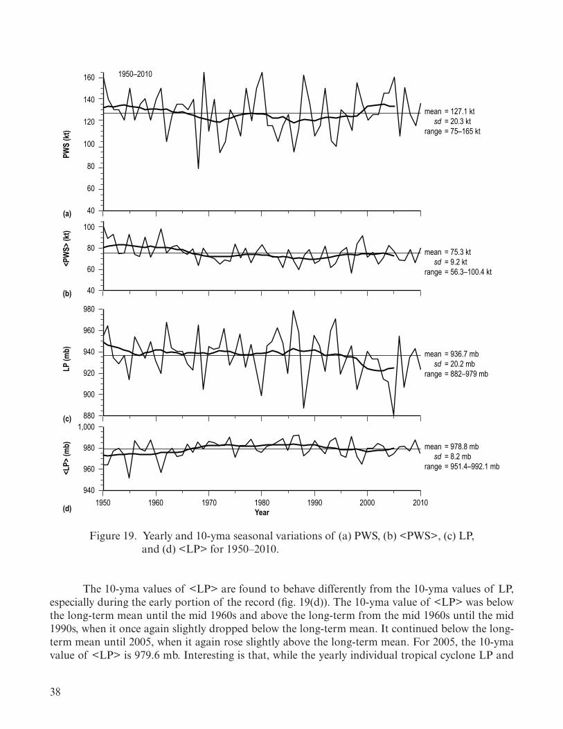
38

mean = 978.8 mb sd = 8.2 mbrange = 951.4–992.1 mb<L

P> (m

b) 980

1,000

960

9401950 1960 1970 1980 1990 2000 2010

Year(d)

mean = 75.3 kt sd = 9.2 ktrange = 56.3–100.4 kt

<PW

S> (k

t)

80

100

60

40(b)

mean = 127.1 kt sd = 20.3 ktrange = 75–165 kt

PWS

(kt)

1950–2010

80

100

120

140

160

60

40(a)

mean = 936.7 mb sd = 20.2 mbrange = 882–979 mbLP

(mb)

920

940

960

980

900

880(c)

Figure 19. Yearly and 10-yma seasonal variations of (a) PWS, (b) <PWS>, (c) LP, and (d) <LP> for 1950–2010.

The 10-yma values of <LP> are found to behave differently from the 10-yma values of LP, especially during the early portion of the record (fig. 19(d)). The 10-yma value of <LP> was below the long-term mean until the mid 1960s and above the long-term from the mid 1960s until the mid 1990s, when it once again slightly dropped below the long-term mean. It continued below the long-term mean until 2005, when it again rose slightly above the long-term mean. For 2005, the 10-yma value of <LP> is 979.6 mb. Interesting is that, while the yearly individual tropical cyclone LP and

39

PWS have shown evidence for considerable strengthening, especially during this second more active interval, overall the yearly mean seasonal <LP> and <PWS> have not demonstrated significant strengthening over time (see below). Hence, the observed variations in <LP> and <PWS> seem more likely due to a multidecadal variation rather than to long-term global warming.

Concerning the observation that the <PWS> has not demonstrated a significant strengthen-ing over time (due to long-term global warming), one can easily show this to be true using the t sta-tistic for independent samples106 and hypothesis testing. For example, during the earlier more active interval 1950–1965 (n = 16), <PWS> is found to average 82.90 kt, having sd = 9.46 kt; during the less active interval 1966–1994 (n = 29), <PWS> is found to average 71.71 kt, having sd = 6.88 kt; and dur-ing the current more active interval 1995–2010 (n = 16), <PWS> is found to average 75.69 kt, hav-ing sd = 9.49 kt. Comparing the earlier more active interval to the less active interval, one computes t = 4.562, which by hypothesis testing suggests that the two intervals are independent (at cl = 99.9%). Comparing the earlier and current more active intervals, one computes t = 2.694, which by hypoth-esis testing again suggests that the two intervals are likewise independent (cl = 98%). Comparing the current more active interval with the preceding less active interval, one computes t = 1.106, which by hypothesis testing suggests that the two intervals are essentially the same (i.e., one must accept the null hypothesis that there exists no statistically significant difference between the two interval means when using <PWS> as the basis for the strengthening of tropical cyclones over time). Hence, the first more active interval appears to be stronger than both the less active interval and the current more active interval (i.e., presently, on the basis of <PWS>, there is no statistical basis for the belief that tropical cyclones are increasing in strength with time).

Regarding the possibility that the number of tropical cyclones not attaining hurricane wind speed during the current more active interval has significantly increased, thereby skewing <PWS> to slightly lower values and, thus, making it appear that the earlier more active interval is the stron-ger, one finds that, on average, during the earlier more active interval 1950–1965, there were about 3.31 ± 1.78 tropical cyclones that did not attain hurricane wind speed (the ±1 sd prediction interval); during the less active interval 1966–1994, on average, there were about 4.17 ± 1.79 tropical cyclones that did not attain hurricane wind speed; and during the current more active interval 1995–2010, on average, there has been about 6.69 ± 2.30 tropical cyclones that did not attain hurricane wind speed. On the basis of the t statistic for independent samples and hypothesis testing, one finds that t = 1.546 when comparing the earlier more active interval with the less active interval, which by hypothesis testing suggests that the two intervals are essentially the same regarding the number of tropical cyclones that did not attain hurricane wind speed. However, when comparing the current more active interval with either the earlier more active interval or the less active interval, one finds t = 4.649 and t = 4.081, respectively, suggesting that indeed the number of tropical cyclones not attaining hurricane wind speed has substantially increased during the current more active interval. Hence, the lower <PWS> now being experienced appears to be due to the increased number of tropical cyclones not attaining hurricane wind speed.

Interestingly, if one examines the <PWS> for major hurricanes only for the three time inter-vals, one finds that the earlier more active interval had 58 major hurricanes having <PWS> = 117.16 ± 15.34 kt, the less active interval had 47 major hurricanes having <PWS> = 118.19 ± 18.75 kt, and the current more active interval has 61 major hurricanes having <PWS> = 120.90 ± 16.24 kt. On

40

the basis of the t statistic for independent samples and hypothesis testing, one finds t = 0.310 when comparing the earlier more active interval with the less active interval, t = 0.804 when comparing the less active interval with the current more active interval, and t = 1.290 when comparing the earlier more active interval with the current more active interval. Thus, although the <PWS> for major hur-ricanes has increased over time, the difference in the means is not yet statistically important, meaning that, presently, one cannot conclude that a strengthening of tropical cyclones has been demonstrated (possibly due to global warming).

Figure 20 displays scatter plots of 10-yma values of (a) LP versus PWS, (b) <LP> versus <PWS>, (c) <PWS> versus PWS, and (d) <LP> versus LP. Significant dfferences are readily appar-ent, especially when the values are separated into two groupings: early (ye, 1950–1989) and current (yc, 1990–2005). For example, for all comparisons, except <LP> versus LP, the inferred regression equations for yc are considered statistically important, being negative (inverse) correlations in fig-ure 20(a) and (b) and a positive (direct) correlation in figure 20(c). Similarly, for all comparisons, except LP versus PWS, the inferred regression equations for ye are considered statistically impor-tant, being negative (inverse) correlations in figure 20(b) and (d) and a positive (direct) correlation in figure 20(c). Interesting is the apparent shift found between ye and yc in figure 20(b). The ye line includes the earlier more active interval and the less active interval, while the yc line includes only the current more active interval. From figure 20(b), one could interpret the scatter plot as indicating that tropical cyclone seasons during the current interval tend to be of lower <LP> for a given <PWS>, as compared to the earlier interval, or, in contrast, that tropical cyclone seasons during the current interval tend to be of lower <PWS> for a given <LP>, as compared to the earlier interval, thereby begging the questions, is there a significant difference in the reliably between the early and current records regarding PWS, <PWS>, LP, and <LP>, or have the parametric relationships truly changed? (Both correlations—ye and yc—are, in fact, inferred to be statistically quite strong, having r = –0.98.)

The same can also be said for figure 20(c). That is, for a given PWS, the <PWS> values dur-ing the current interval are considerably lower than those found in the earlier interval, although the inferred correlation for the earlier interval is the stronger, having r = 0.95 as compared to r = 0.79.

Figure 21 depicts scatter plots of 10-yma values of each of the parameters against 10-yma values of <ONI> (left-most panels), <SOI> (middle-left panels), <NAO> (middle-right panels), and <AT> (right-most panels). Only the inferred regression line for the current interval (yc) is plotted. All correlations are inferred to be statistically important, with the stronger correlations usually being the ones against <AT>. Thus, for the current interval, higher (lower) PWS and <PWS> occur with higher (lower) <AT>, while lower (higher) LP and <LP> occur with higher (lower) <AT>. Like-wise, higher (lower) PWS and <PWS> occur with lower (higher) <ONI> and <NAO>, in particular the latter, while lower (higher) LP and <LP> occur with lower (higher) <ONI> and <NAO>. For <SOI>, higher (lower) PWS and <PWS> occur with higher (lower) <SOI>, while lower (higher) LP and <LP> occur with higher (lower) <SOI>. Thus, by monitoring the 10-yma values of the ENSO indices and the surface air temperature at Armagh Observatory, one might be able to better determine the likelihood of the occurrence of stronger tropical cyclones during the yearly hurricane season. As an example, if the 10-yma of <AT> = 10.02 ºC for 2006 (i.e., fd<AT>10 = 0, indicating the same value for <AT>10 in 2006 as was observed for 2005), then the 2006 values for (PWS)10, <PWS>10, (LP)10, and <LP>10 are, respectively, 131.2 ± 1.7 kt, 74.1 ± 0.9 kt, 926.5 ± 2.9 mb, and

41

<LP>

10

65 70 858075<PWS>10(b)

980

975

970

985ye = 1,045.9757 – 0.8814xr = –0.979, r2 = 0.957se = 1.724, cl >99.9%

yc = 1,045.5615 – 0.9123xr = –0.983, r2 = 0.966se = 1.389, cl >99.9%

<LP>

10

900 925 1,000975950(LP)10

(d)

980

975

970

985

ye = 1,425.0736 – 0.4744xr = –0.294, r2 = 0.086se = 3.458, cl >95%

yc = 818.6824 + 0.1720xr = 0.763, r2 = 0.583se = 6.375, cl <90%

yc

ye

(LP)

10

115 120 135130125(PWS)10(a)

950

925

900

975

1,000

ye = 929.0701 + 0.0888xr = 0.178, r2 = 0.032se = 2.633, cl <90%

yc = 1,095.5722 – 1.2887xr = –0.998, r2 = 0.996se = 1.759, cl >99.9%

<PW

S>10

115 120 135130125(PWS)10

(c)

75

70

65

80

85

ye = –31.0969 + 0.8486xr = 0.952, r2 = 0.907se = 1.386, cl >99.9%

yc = 41.5117 + 0.2476xr = 0.790, r2 = 0.624se = 1.016, cl >99.9%

yc

yc

ye

ye

ycye

Figure 20. Scatter plots: (a) (LP)10 vs. (PWS)10; (b) <LP>10 vs. <PWS>10; (c) <PWS>10 vs. (PWS)10; and (d) <LP>10 vs. (LP)10.

977.9 ± 0.6 mb (±1 se prediction intervals). This suggests that the 10-yma value for PWS in 2006 will remain above the long-term mean and that the 2011 value of PWS should be within the range 55 to 123 kt; the 10-yma value for <PWS> in 2006 will remain below the long-term mean and that the <PWS> value for 2011 should be within the range 80 to 116 kt; the 10-yma value for LP in 2006 will remain below the long-term mean and that the LP value for 2011 should be within the range 924 to 1,040 mb; and the 10-yma value of <LP> in 2006 will be near the long-term mean and that the 2011 value of <LP> should be within the range 937 to 961 mb. A higher 10-yma value of <AT> for 2006 will increase the likelihood of a higher PWS and <PWS> and a lower LP and <LP> in 2006 (and quite possibly in 2011), while a lower 10-yma value of <AT> for 2006 will increase the likeli-hood of a lower PWS and <PWS> and a higher LP and <LP> in 2006 (and quite possibly in 2011).

42

<LP>

10

–0.5 0 0.5<ONI>10(d)

980

975

970

985

yc = 977.385 + 10.095xr = 0.668, r2 = 0.447se = 1.170, cl >99.5%

yc = 978.100 + 8.996xr = 0.788, r2 = 0.620se = 0.890, cl >99.9%

yc

(LP)

10

(c)

950

925

975

1,000

yc = 922.926 + 55.917xr = 0.834, r2 = 0.696se = 4.027, cl >99.9%

yc

<PW

S>10

(b)

75

70

65

80

85

yc = 74.877 – 11.975xr = –0.736, r2 = 0.542se = 1.220, cl >99.8%

yc

(PW

S)10

(a)

125

120

115

130

135

yc = 133.817 – 42.420xr = –0.817, r2 = 0.668se = 3.286, cl >99.9%

yc

–5 0 5<SOI>10

yc = 977.577 – 0.623xr = –0.668, r2 = 0.446se = 1.621, cl >95%

yc

yc

–0.5 0 0.5<NAO>10

yc

yc = 927.260 + 46.062xr = 0.909, r2 = 0.826se = 3.093, cl >99.9%

yc = 923.135 – 3.829xr = –0.924, r2 = 0.854se = 3.014, cl >99.9%

yc

yc = 74.635 + 0.733xr = 0.729, r2 = 0.531se = 1.208, cl >99.8%

yc

yc = 133.689 + 2.919xr = 0.910, r2 = 0.828se = 2.389, cl >99.9%

yc

yc = 73.988 – 10.255xr = –0.833, r2 = 0.694se = 0.982, cl >99.9%

yc

yc = 130.512 – 34.771xr = –0.886, r2 = 0.785se = 2.638, cl >99.9% yc

yc

yc = 1,039.3603 – 6.1301xr = –0.839, r2 = 0.703se = 0.618, cl >99.9%

9 9.5 10<AT>10

yc

yc = 1,238.347 – 31.126xr = –0.960, r2 = 0.921se = 2.887, cl >99.9%

yc

yc = 5.851 + 6.816xr = 0.866, r2 = 0.749se = 0.754, cl >99.9%

yc = –106.946 + 23.763xr = 0.946, r2 = 0.895se = 1.689, cl >99.9%

yc

Figure 21. Scatter plots of (PWS)10, <PWS>10, (LP)10, and <LP>10 vs. left-most panels, <ONI>10; left-middle panels, <SOI>10; middle-right panels, <NAO>10; and right-most panels <AT>10.

43

Figure 22 shows the variation of the fd values of the 10-yma values of (a) PWS, (b) <PWS>, (c) LP, and (d) <LP>. Runs-testing suggests that fd(PWS)10 and fd(<LP>)10 are nonrandomly dis-tributed, having z = –4.80 and –2.21, respectively, and that fd(<PWS>)10 and fd(LP)10 are randomly distributed, having z = –1.71 and –1.13, respectively. A positive fd(PWS)10 value means that the 10-yma of PWS for 2006 will be >132.3 kt and that PWS for 2011 will be ≥113 kt (130 mph), while a negative value means that the 10-yma value of PWS for 2006 will be <132.3 kt and that PWS for 2011 will be ≤109 kt (125 mph). The 2006 value for fd(PWS)10 is expected to lie between –1.8 and 2.7, since these values result in PWS for 2011 of 75 and 165 kt, respectively, which are the previously observed extremes for PWS during the interval 1950–2010. Similarly, a positive fd(<PWS>)10 value means that the 10-yma of <PWS> for 2006 will be >72.6 kt and that <PWS> for 2011 will be ≥69.6 kt (80 mph), while a negative value means that the 10-yma value of <PWS> for 2006 will be <72.6 kt and that <PWS> for 2011 will be ≤65.6 kt (76 mph). The 2006 value for fd(<PWS>)10 is expected to lie between –0.57 and 1.64, since these values result in <PWS> for 2011 of 56.3 and 100.4 kt, respec-tively, which are the previously observed extremes for <PWS> during the interval 1950–2010. Like-wise, a positive fd(LP)10 value means that the 10-yma of LP for 2006 will be >925 mb and that LP for 2011 will be ≥954 mb, while a negative value means that the 10-yma value of LP for 2006 will be <925 mb and that LP for 2011 will be ≤950 mb. The 2006 value for fd(LP)10 is expected to lie between –3.5 and 1.35, since these values result in LP for 2011 of 882 and 979 mb, respectively, which are the previously observed extremes for LP during the interval 1950–2010. Lastly, a positive fd(<LP>)10 value means that the 10-yma of <LP> for 2006 will be >979.6 mb and that <LP> for 2011 will be ≥985.1 mb, while a negative value means that the 10-yma value of <LP> for 2006 will be <979.6 mb and that <LP> for 2011 will be ≤981.1 mb. The 2006 value for fd(<LP>)10 is expected to lie between –1.585 and 0.45, since these values result in PWS for 2011 of 951.4 and 992.1 mb, respectively, which are the previously observed extremes for <LP> during the interval 1950–2010.

2.6 Statistical Aspects of the Differences (Yearly Value Minus the 10-yma Value)

As mentioned in section 2.1, one can use the difference between the yearly value and the same year expected 10-yma value to crudely forecast the level of tropical cyclone activity during the cur-rent hurricane season. Figure 23 displays the variation of differences for (a) NTC, (b) NH, (c) NMH, and (d) NUSLFH. Recall that the difference is merely the yearly value minus the 10-yma value for the same year (i.e., d(x) = x – x10, where x is the parameter of interest). For 2005, d(NTC) = 28 – 15.3 = 12.7, d(NH) = 15 – 7.8 = 7.2, d(NMH) = 7 – 3.7 = 3.3, and d(NUSLFH) = 6 – 1.9 = 4.1. Runs-testing suggests that the all differences are distributed randomly, except the one for d(NTC).

Examination of figure 23(a) reveals that, for d(NTC), 39 of 56 years (70%) have differences within the range 0 ± 3 and 52 of 56 years (93%) have differences within the range 0 ± 5. During the current interval, 9 of 16 years (56%) and 14 of 16 years (88%), respectively, have differences within the same stated ranges. Hence, statistically speaking, one expects d(NTC) for 2006 to lie within these stated ranges, unless the year 2006 proves to be another statistical outlier year with respect to this parameter, thereby inferring NTC10 = 10 ± 3 or 10 ± 5 for 2006, where 10 is the known NTC value for 2006. However, such values imply NTC ≤5 for 2011 (based on NTC10 = 15). Because the usual fd(NTC)10 = 0.1 ± 0.3 (the ±1 sd prediction interval; see fig. 2), true for 49 of 55 years (89%) for the interval 1950–2004, and 10 of 15 years (67%) during the current interval 1990–2004, one expects NTC10 = 15.3 ± (0.1 ± 0.3) for 2006, or about 15.1–15.7, a range of values just outside-high

44

mean = 0.12 sd = 0.71range = –1.2 to 2.1fd

(<LP

> 10)

–3

–1.5

3

0

1.5

1950 1960 1970 1980 1990 2000Year(d)

mean = –0.44 sd = 1.79range = –5.3 to 2.8

fd(L

P 10)

–5

2.5

5

–2.5

0

(c)

mean = –0.14 sd = 0.77range = –1.9 to 1.5fd

(PW

S 10)

–2

2

1

–1

0

(b)

mean = 0.01 sd = 1.68range = –3.5 to 4.7fd

(PW

S 10)

1950–2004

–5

5

2.5

–2.5

0

(a)

Figure 22. Yearly variation of (a) fd(PWS10), (b) fd(<PWS>10), (c) fd(LP10), and (d) fd(<LP>10) for 1950–2004.

45

mean = 0.03 sd = 1.45range = –2.3 to 4.4

d(NU

SLFH

)

5

0

–51950 1960 1970 1980 1990 2000

Year(d)

1950–2005

na = 21nb = 35nra = 14

⇒ z = 0.29⇒ random distribution

mean = 0.15 sd = 1.71range = –2.1 to 3.9

d(NM

H)

5

0

–5(c)

na = 27nb = 29nra = 17

⇒ z=1.35⇒random distribution

mean = 0.10 sd = 2.43range = –4.0 to 7.2

d(NH

)

5

10

0

–5(b)

na = 29nb = 27nra = 15

⇒ z=0.27⇒ random distribution

mean = 0.14 sd = 3.34range = –5.1 to 12.7

d(NT

C)

0

5

10

15

–5

–10(a)

na = 29nb = 27nra = 19

⇒ z=2.39 ⇒nonrandom distribution

Figure 23. Yearly variation of (a) d(NTC), (b) d(NH), (c) d(NMH), and (d) d(NUSLFH) for 1950–2005.

the expected range deduced from the differences, values that suggest NTC = 7–19 for 2011. Given that the phase of ENSO probably will be in the neutral state (or perhaps LN-like) and that the majority of outlier years have occurred during the current interval, it appears likely then that the year 2011 will be another outlier year (with respect to this parameter), inferring fd(NTC)10 > 0 for 2005, (NTC)10 > 15.3 for 2006, and NTC ≥ 13 for 2011. (Recall that NTC10 must be ≥14.75 in 2006,

46

since that value implies NTC = 0 for 2011. Also, because NTC has never dipped below 4 over the past 61 years, NTC10 very probably will be ≥14.95. For NTC in 2011 to be equal to the long-term average of 11 tropical cyclones, NTC10 must be equal to 15.30, and for NTC in 2011 to be equal to the cur-rent average of 15 during this second more active interval, NTC10 must be equal to 15.50, inferring fd(NTC)10 = 0.2 for 2005.)

Because the distributions of d(NH), d(NMH), and d(NUSLFH) are all found to be randomly distributed (based on runs-testing), for convenience, the following discussion of the differences will be based on 50% and 90% prediction intervals, rather than specific difference values (i.e., ±3 or ±5). For example, for d(NH), the 50% prediction interval is about 0 ± 1.6 and the 90% prediction interval is about 0 ± 4.1. Examination of figure 23(b) reveals that 30 of 56 years (54%) have d(NH) = 0 ± 1.6 (5 of 16, or 31%, for the current interval) and 52 of 56 years (93%) have d(NH) = 0 ± 4.1 (14 of 16 years, or 88%, for the current interval). Hence, statistically speaking, one expects d(NH) for 2006 to lie within these same stated ranges, unless the year 2006 proves to be another statistical outlier year with respect to this parameter, inferring NH10 = 5 ± 1.6 or 5 ± 4.1 for 2006, where 5 is the NH for 2006. A value of NH10 = 7.70 in 2006 is required for NH = 3 in 2011 (NH = 3 being the lowest value observed for the past 61 years, having occurred in 1957, 1962, 1972, 1983, 1987, 1994, 1997, and 2009, many of these years being associated with EN episodes). A value of NH10 = 7.85 in 2006 is required for NH = 6 in 2011 (NH = 6 being the long-term mean for the interval 1950–2010), and a value of NH10 = 7.95 in 2006 is required for NH = 8 in 2011 (NH = 8 being the average during the current interval 1995–2010). It appears then that, based on d(NH), the value of NH10 in 2006 should be ≥7.70, possibly ≥7.95. Now, because the usual fd(NH)10 = 0 ± 0.2, true for 40 of 55 years (73%), or 9 of 15 years (60%) during the current interval, NH10 should be equal to about 7.8 ± 0.2 for 2006 (i.e., 7.6–8), inferring NH = 1–9 for 2011 (a higher NH10 in 2006 implies a higher NH in 2011, while a lower value of NH10 in 2006 implies a lower NH for 2011). Combining the difference and usual fd values, clearly, one expects NH10 = 7.85 ± 0.15 for 2006 and NH ≥ 3 in 2011 (i.e., NH = 3–9, possibly higher, given that the expected phase of ENSO is N or LN-like for 2011).

For d(NMH), the 50% and 90% prediction intervals are, respectively, about 0 ± 1.2 and 0 ± 2.9. Examination of figure 23(c) reveals that 27 of 55 years (49%) have d(NMH) = 0 ± 1.2 (7 of 16 years, 44%, for the current interval) and 50 of 55 years (91%) have d(NMH) = 0 ± 2.9 (14 of 16 years, 88%, for the current interval). Hence, statistically speaking, one expects d(NMH) for 2006 to lie within these same stated ranges, unless the year 2006 proves to be a statistical outlier year with respect to this parameter, inferring NMH10 = 2 ± 1.2 or 2 ± 2.9 for 2006 (i.e., NMH10 ≥ 0). A value of NMH10 = 3.6 in 2006 is the smallest value possible, since that value implies NMH = 0 in 2011. A value of NMH10 = 3.75 in 2006 yields NMH = 3 in 2011 (NMH = 3 being the long-term mean), while a value of NMH10 = 3.8 in 2006 yields NMH = 4 in 2011 (NMH = 4 being the average for the current interval). It appears then that, based on d(NMH), the value of NMH10 in 2006 should be ≥3.6, quite possibly larger. Now, because the usual fd(NMH)10 = 0 ± 0.2, true for 46 of 55 years (84%), or 11 of 15 years (73%) during the current interval, this suggests that NMH10 = 3.7 ± 0.2 for 2006, or about 3.5–3.9. Combining the difference and usual fd values, clearly, one expects NMH10 = 3.75 ± 0.15 (or higher) in 2006, inferring NMH = 0–6 in 2011. Given that the phase of ENSO will probably be in the neutral state (or perhaps LN-like), this seems to suggest that fd(NMH)10 > 0 for 2005, (NMH)10 > 3.7 for 2006, and NMH ≥ 3 for 2011.

47

For d(NUSLFH), the 50% and 90% prediction intervals are, respectively, about 0 ± 1 and 0 ± 2.5. Examination of figure 23(d) reveals that 33 of 55 years (60%) have d(NUSLFH) = 0 ± 1 (7 of 16 years, 44%, for the current interval) and 53 of 55 years (96%) have d(NUSLFH) = 0 ± 2.5 (14 of 16 years, 88%, for the current interval). Hence, statistically speaking, one expects d(NUSLFH) for 2006 to lie within these same stated ranges, unless the year 2006 proves to be a statistical outlier year with respect to this parameter, inferring NUSLFH10 = 0 ± 1 or 0 ± 2.5 for 2006 (i.e., NUSLFH10 ≥ 0). A value of NUSLFH10 = 1.9 in 2006 is the smallest value possible, since that value implies NUSLFH = 0 in 2011. A value of NUSLFH10 = 1.95 in 2006 yields NUSLFH = 1 in 2011 (NUSLFH = 1 being the most frequently observed yearly frequency), while a value of NUSLFH10 = 2.2 in 2006 yields NUSLFH = 6 in 2011 (NUSLFH = 6 being the largest observed yearly frequency). It appears then that, based on d(NUSLFH), the value of NUSLFH10 in 2006 will be ≥1.9. Now, because the usual fd(NUSLFH)10 = 0 ± 0.2, true for 50 of 55 years (91%), or 13 of 15 years (87%) during the current interval, this suggests that NUSLFH10 = 1.9 ± 0.2 for 2006, or about 1.7–2.1. Combining the differ-ence and usual fd values, clearly, one expects NUSLFH10 = 1.95 ± 0.05 (or higher) in 2006, inferring NUSLFH = 0–2 for 2011. Given that the phase of ENSO will probably be in the neutral state (or perhaps LN-like), this seems to suggest that fd(NUSLFH)10 > 0 for 2005, (NUSLFH)10 > 1.9 for 2006, and NUSLFH ≥ 1 for 2011. (Recall that over the past 61 years, there has never been a single occurrence of three consecutive years of NUSLFH = 0. Because NUSLFH = 0 in 2009 and 2010, NUSLFH ≥ 1 is highly anticipated for the 2011 hurricane season.)

Differences can also be employed for a crude estimation of the surface air temperature and ENSO indices, as well as the peak wind speed and lowest pressure values and latitude and longitude location onset values. Figure 24 displays the variation of the differences for (a) <AT>, (b) <ONI>, (c) <SOI>, and (d) <NAO>, and figures 25 and 26 depict the differences as related to the latitude and longitude location onset values and to the peak wind speed and lowest pressure values, respectively. Runs-testing suggests that all of the difference values are randomly distributed, except the one for d(<NAO>). (Discussion will be limited here to only the difference values for the surface air tem-perature and the ENSO indices since they appear to be useful factors for determining the frequency of tropical cyclones during a typical hurricane season. The differences as related to the latitude and longitude location onset values and to the peak wind speeds and lowest pressures are shown only for completeness.)

Examination of figure 24(a) reveals that, for d(<AT>), 27 of 56 years (48%) have d(<AT>) = –0.03 ± 0.27 ºC and 50 of 56 years (89%) have d(<AT>) = –0.03 ± 0.67 ºC (i.e., the 50% and 90% prediction intervals, respectively). Hence, statistically speaking, one expects d(<AT>) for 2006 to lie within these same stated ranges, unless the year 2006 proves to be a statistical outlier year with respect to this parameter, inferring <AT>10 = 10.43 ± (–0.03 ± 0.27) ºC or 10.43 ± (–0.03 ± 0.67) ºC for 2006, where 10.43 ºC is the <AT> for 2006. Therefore, based on d(<AT>), one expects <AT>10 to lie within the range 10.13 to 10.67 ºC (with 50% accuracy) or within the range 9.73 to 11.17 ºC (with 90% accuracy) in 2006. However, as previously noted, because fd(<AT>)10 = 0 ± 0.05 ºC (true for 40 of 55 years, or 73%, for the interval 1950–2004, and true for 7 of 15 years, or 47%, for the current interval 1990–2004), one expects <AT>10 = 10.02 ± 0.05 ºC in 2006, where 10.02 ºC is the 10-yma value of <AT> for 2005, inferring <AT> = 10.75 ± 1 ºC in 2011, a value about 1 ºC warmer (or more) than was seen in 2010 (8.74 ºC), possibly becoming a new record high for Armagh Obser-vatory (10.59 ºC is the present record high in 2007; a value of <AT>10 > 10.01 ºC in 2006 indicates a new record value in 2011).

48

mean = 0 sd = 0.31range = –0.83 to 0.60d(

<NAO

>)

0

0.5

1

–0.5

–11950 1960 1970 1980 1990 2000

Year(d)

1950–2005

na = 26nb = 25nra = 17

na = 26nb = 30nra = 12

na = 24nb = 27nra = 12

na = 31nb = 25nra = 15

⇒ z=2.08 ⇒ nonrandom distribution

mean = –0.19 sd = 6.45range = –10.8 to 11.4d(

<SOI

>)

–5

0

5

10

15

–10

–15(c)

⇒ z=–1.03 ⇒ random distribution

mean = 0 sd = 0.61range = –1.16 to 1.15

d(<O

NI>)

–0.5

0

0.5

1

1.5

–1

–1.5(b)

⇒ z=–0.66 ⇒ random distribution

mean = –0.03 sd = 0.40range = –0.85 to 0.80

d(<A

T>)

0

0.5

1

–0.5

–1(a)

⇒ z=0.32 ⇒ random distribution

Figure 24. Yearly variation of (a) d(<AT>), (b) d(<ONI>), (c) d(<SOI>), and (d) d(<NAO>) for 1950–2005.

49

mean = 0.37 sd = 5.65range = –9.0 to 12.4

d(<L

ONG>

)

0

5

10

15

–5

–101950 1960 1970 1980 1990 2000

Year(b)

1950–2005

na = 25nb = 31nra = 18

⇒z=2.00 ⇒random distribution

mean = 0.02 sd = 2.87range = –4.8 to 6.5

d(<L

AT>)

0

5

10

–5

–10(a)

na = 25nb = 31nra = 15

⇒z =0.38 ⇒random distribution

Figure 25. Yearly variation of (a) d(<LAT>) and (b) d(<LONG>) for 1950–2005.

For d(<ONI>) (fig. 24(b)), 22 of 51 years (43%) have d(<ONI>) = 0 ± 0.41 and 46 of 51 years (90%) have d(<ONI>) = 0 ± 1.02 (i.e., the 50% and 90% prediction intervals, respectively). Hence, statistically speaking, one expects d(<ONI>) for 2006 to lie within these same stated ranges, unless the year 2006 proves to be a statistical outlier year with respect to this parameter, inferring <ONI>10 = 0.25 ± 0.41 or 0.25 ± 1.02 for 2006, where 0.25 is the <ONI> for 2006. Therefore, based on d(<ONI>), one expects <ONI>10 to lie within the range –0.16 to 0.66 (with 50% accuracy) or within the range –0.77 to 1.27 (with 90% accuracy) in 2006. However, because fd(<ONI>)10 = 0 ± 0.05 (true for 34 of 50 years, or 68%, for the interval 1955–2004, and true for 12 of 15 years, or 80%, for the current interval 1990–2004), one expects <ONI>10 = 0.04 ± 0.05 in 2006 (i.e., about –0.01 to 0.09), inferring <ONI> = 2.56 ± 1 ºC for 2011.

For d(<SOI>) (fig. 24(c)), 23 of 56 years (41%) have d(<SOI>) = –0.19 ± 4.37 and 53 of 56 years (95%) have d(<SOI>) = –0.19 ± 10.82 (i.e., the 50% and 90% prediction intervals, respec-tively). Hence, statistically speaking, one expects d(<SOI>) for 2006 to lie within these same stated ranges, unless the year 2006 proves to be a statistical outlier year with respect to this parameter, infer-ring <SOI>10 = –1.9 – (–0.19 ± 4.37) or –1.9 – (–0.19 ± 10.82) for 2006, where –1.9 is the <SOI> for 2006. Therefore, based on d(<SOI>), one expects <SOI>10 to lie within the range –6.08 to 2.66 (with 50% accuracy) or within the range –12.53 to 9.11 (with 90% accuracy) in 2006. However, because

50

mean = –0.31 sd = 7.40range = –22.9 to 13.7

d(<L

P>)

30

0

–301950 1960 1970 1980 1990 2000

Year

1950–2005

(d)

na = 28nb = 28nra = 14

⇒ z = –0.27 ⇒ r andom distribution

mean = –0.87 sd = 19.28range = –52.3 to 35.8

d(LP

)

50

0

–50(c)

na = 30nb = 26nra = 14

⇒ z = –0.25 ⇒ random distribution

mean = 0.50 sd = 8.15range = –17.1 to 19.9

mean = 0.79 sd = 19.51range = –48.3 to 43.2

d(<P

WS>

)d(

PWS)

0

50

–50

–20

20

0

(b)

(a)

na = 28nb = 28nra = 16

⇒ z = 0.80 ⇒ random distribution

na = 29nb = 27nra = 18

⇒ z = 1.86 ⇒ random distribution

Figure 26. Yearly variation of (a) d(PWS), (b) d(<PWS>), (c) d(LP), and (d) d(<LP>) for 1950–2005.

fd(<SOI>)10 = 0 ± 0.5 (true for 30 of 55 years, or 55%, for the interval 1950–2004, and true for 10 of 15 years, or 67%, for the current interval 1990–2004), one expects <SOI>10 = 0.13 ± 0.5 in 2006 (i.e., about –0.37 to 0.63), inferring <SOI> = –1.5 ± 10 for 2011.

For d(<NAO> (fig. 24(d)), 33 of 51 years (65%) have d(<NAO>) = 0 ± 0.30 and 45 of 51 years (88%) have d(<NAO>) = 0 ± 0.50. Hence, statistically speaking, one expects d(<NAO>) for 2006 to lie within these same stated ranges, unless the year 2006 proves to be a statistical outlier year with

51

respect to this parameter, inferring <NAO>10 = –0.21 ± 0.3 or –0.21 ± 0.5 for 2006, where –0.21 is the <NAO> for 2006. Therefore, based on d(<NAO>), one expects <NAO>10 to lie within the range –0.51 to 0.09 or –0.71 to 0.29 in 2006. However, because fd(<NAO>)10 = 0 ± 0.05 (true for 45 of 55 years, or 82%, for the interval 1950–2004, and true for 14 of 15 years, or 93%, for the current inter-val 1990–2004), one expects <NAO>10 = –0.12 ± 0.05 in 2006 (i.e., about –0.17 to –0.07), inferring <NAO> = 1.18 ± 1 for 2011.

2.7 Estimating <AT>, <ONI>, <SOI>, and <NAO> for 2011 From Their Early Observed Monthly Values in 2011

Figure 27 displays the monthly values of (a) AT and (b) ONI for the early portion of 2011 (the filled circles), in comparison to the mean values and extremes for the interval 1995–2010. Through March 2011, AT appears to be progressing along the mean curve, suggesting that the yearly mean for 2011 will be about 10 ºC, up from the 2010 value of 8.74 ºC, but one that will not be record-breaking (i.e., an <AT> in 2011 <10.59 ºC). Also, ONI values appear to be slowly returning to more neutral-like values later in the year from its current LN-like values. Both AT and ONI values are within their 1995–2010 extreme limits, suggesting that, at least for this juncture, the year 2011 does not appear to be destined to be a year of record warmth or indicative of a prolonged LN episode. (Regarding AT, because the highest temperatures for the year typically occur in July and August, one must remain open to the possibility that the year 2011 could become a year of record warmth, at least, until tem-peratures for July and August are recorded.)

Figure 28 compares the monthly values of SOI for 2011 (through April) with the 1995–2010 mean and extreme values. Unlike AT and ONI, the SOI monthly values are currently higher than any of the previous SOI monthly values observed over the past 16 years. Is this an indication that the current ongoing LN will indeed persist longer than the usual spring ending of most ENSO events, perhaps, extending into summer or even persisting into next year?

Figure 29 compares the monthly values of NAO for 2011 (through April) with the 1995–2010 mean and extreme values. The behavior of NAO remained within the limits of the 1995–2010 extremes (like AT and ONI) during January through March; however, in April it moved well outside-high the upper extreme (positive) April value. Is this an indication that NAO will be positive in value for 2011?

Table 11 gives the inferred statistical regressions for estimating the yearly mean parametric values for the year 2011 based on monthly averages from January through August. As an exam-ple, AT for January 2011 measured 3.5 ºC. Based on the inferred correlation using the January value (i.e., table 11, using AT(1), having r = 0.569), one computes the 90% prediction interval to be <AT> = 9.65 ± 0.72 ºC for 2011. Based on the average (5.2 ºC) of the January (3.5 ºC) and February (6.9 ºC) values, one computes (i.e., table 11, using the AT(2), having r = 0.725) the 90% prediction interval to be <AT> = 9.96 ± 0.64 ºC for 2011, and so on. For <AT>, all inferred correlations are statistically important. For <ONI>, the inferred correlations do not become statistically important until ONI(6), meaning knowing the average ONI for January–June; for <SOI>, the inferred cor-relations do not become statistically important until SOI(5), meaning knowing the average SOI for January–May; and for <NAO>, the inferred correlations become statistically important at NAO(2),

52

mean (1995–2010) (0.06 °C)

lower extreme

EN-like

LN-like

upper extrememean (1995–2010) (10 °C)

lower extreme

upper extreme

ONI (

mon

thly

in °C

)AT

(mon

thly

in °C

)

–1.5

–1

–0.5

0

0.5

1

1.5

2

2.5

0

5

10

15

20

–2J F M A M J J A S O N D

Calendar Month(b)

(a)

Figure 27. Comparison of 2011 monthly values against the 1995–2010 monthly mean and extremes of (a) Armagh Observatory surface air temperature and (b) the Oceanic Niño Index.

53

mean (1995–2010) (0.5)

lower extreme

upper extreme

EN-like

LN-like

SOI (

mon

thly)

–25

–20

–15

–10

–5

0

5

10

15

20

25

30

–30J F M A M J J A S O N D

Calendar Month

Figure 28. Comparison of 2011 monthly values against the 1995–2010 monthly mean and extremes of the Southern Oscillation Index.

54

mean (1995–2010) (–0.14)

lower extreme

upper extreme

NAO

(mon

thly)

–2.5

–2

–1.5

–1

–0.5

1

1.5

2

2.5

3

–3J F M A M J J A S O N D

Calendar Month

0

0.5

Figure 29. Comparison of 2011 monthly values against the 1995–2010 monthly mean and extremes of the North Atlantic Oscillation Index.

55

Table 11. Inferred statistical regressions between <AT>, <ONI>, <SOI>, and <NAO> against their running monthly means based on 1995–2010.

Regression Equation r r×r se cl(%) 2011 ±50%PI ±90%PI<AT> = 8.911 + 0.211AT(1) 0.569 0.324 0.408 >95 9.65 0.28 0.72<AT> = 8.292 + 0.321AT(2) 0.725 0.526 0.366 >99.5 9.96 0.25 0.64<AT> = 7.941 + 0.353AT(3) 0.716 0.513 0.371 >99.5 9.97 0.26 0.65<AT> = 6.801 + 0.485AT(4) 0.768 0.590 0.352 >99.9 0.24 0.62<AT> = 5.748 + 0.563AT(5) 0.775 0.601 0.291 >99.9 0.20 0.51<AT> = 3.623 + 0.738AT(6) 0.794 0.631 0.331 >99.9 0.23 0.58<AT> = 0.683 + 0.965AT(7) 0.857 0.735 0.293 >99.9 0.20 0.52<AT> = –0.762 + 1.032AT(8) 0.897 0.805 0.320 >99.9 0.22 0.56

<ONI> = 0.054 + 0.158ONI(1) 0.317 0.100 0.579 <90 –0.15 0.40 1.02<ONI> = 0.058 + 0.183ONI(2) 0.338 0.114 0.575 <90 –0.16 0.40 1.01<ONI> = 0.059 + 0.217ONI(3) 0.358 0.128 0.570 <90 –0.19 0.39 1.00<ONI> = 0.058 + 0.271ONI(4) 0.397 0.157 0.561 <90 0.39 0.99<ONI> = 0.053 + 0.368ONI(5) 0.469 0.220 0.539 >90 0.37 0.95<ONI> = 0.040 + 0.509ONI(6) 0.570 0.325 0.502 >95 0.35 0.88<ONI> = 0.020 + 0.685ONI(7) 0.686 0.471 0.444 >99.5 0.31 0.70<ONI> = 0.001 + 0.866ONI(8) 0.802 0.643 0.365 >99.9 0.25 0.64

<SOI> = 0.334 + 0.138SOI(1) 0.237 0.056 6.281 <90 3.08 4.35 11.06<SOI> = 0.378 + 0.108SOI(2) 0.189 0.036 6.349 <90 2.79 4.39 11.18<SOI> = 0.380 + 0.159SOI(3) 0.258 0.067 6.246 <90 3.79 4.32 11.00<SOI> = 0.371 + 0.274SOI(4) 0.437 0.191 5.814 >90 6.20 4.02 10.24<SOI> = 0.697 + 0.432SOI(5) 0.565 0.319 5.334 >95 3.69 9.39<SOI> = 0.919 + 0.610SOI(6) 0.687 0.472 4.694 >99.5 3.25 8.27<SOI> = 0.871 + 0.826SOI(7) 0.797 0.635 3.908 >99.9 2.70 6.88<SOI> = 1.011 + 0.982SOI(8) 0.892 0.796 2.916 >99.9 2.02 5.14

<NAO> = –0.200 + 0.183NAO(1) 0.339 0.115 0.353 <90 –0.36 0.24 0.62<NAO> = –0.238 + 0.325NAO(2) 0.578 0.334 0.306 >98 –0.27 0.21 0.54<NAO> = –0.249 + 0.404NAO(3) 0.663 0.439 0.281 >99 0.00 0.19 0.49<NAO> = –0.236 + 0.587NAO(4) 0.759 0.577 0.244 >99.9 0.19 0.17 0.43<NAO> = –0.182 + 0.610NAO(5) 0.843 0.711 0.201 >99.9 0.14 0.35<NAO> = –0.128 + 0.686NAO(6) 0.888 0.789 0.172 >99.9 0.12 0.30<NAO> = –0.238 + 0.325NAO(7) 0.872 0.761 0.183 >99.9 0.13 0.32<NAO> = –0.238 + 0.325NAO(8) 0.873 0.763 0.183 >99.9 0.13 0.32

Note: The numbers in parentheses (e.g., (1), (2), (3), ...) refer to parametric values for January, (January + Febuary)/2, (January + Febuary + March)/3, ..., respectively).

56

meaning knowing the average NAO for January–February (which is presently known and indi-cates <NAO> = –0.27 ± 0.54 for 2011; using NAO(4), one computes the 90% prediction interval to be <NAO> = 0.19 ± 0.43 for 2011). As the year progresses, clearly, one can more accurately gauge the yearly parametric mean values, which can then be used to infer the likely 10-yma parametric values (and expected frequencies of tropical cyclones for 2011 and other ancillary parametric values) and differences for 2006, which in turn can be used to infer the fd parametric values for 2005.

57

3. SUMMARY

Between 1995 and 2010, inclusive, the mean yearly (seasonal) frequency of tropical cyclones in the North Atlantic Basin has been about 54% greater than what occurred during the earlier interval 1950–1994, the mean yearly frequency of hurricanes is about 41% greater, the mean yearly frequency of major (or intense) hurricanes is about 63% greater, and the mean yearly frequency of land-falling hurricanes along the U.S. coastline is about 30% greater. This enhanced level of activity appears to be driven by a multidecadal variation, although global warming also appears to contribute.

For the interval 1995–2010, the number of tropical cyclones has averaged about 15 storms per year, having an sd of about 5 storms per year and a range of 8 to 28 storms per year, with 9 of the 16 years (56%) having a frequency of 15 or more storms per year, including the years 1995, 2000, 2001, 2003, 2004, 2005, 2007, 2008, and 2010. The 10-yma value of the number of tropical cyclones per year possibly has attained a plateau of about 15 storms per year in the years 2003–2005.

During the same interval, the number of hurricanes has averaged about 8 storms per year, having an sd of about 3 storms per year and a range of 3 to 15 storms per year, with 4 of the 16 years (25%) having a frequency of 10 or more storms per year, including the years 1995, 1998, 2005, and 2010. The 10-yma value of the number of hurricanes per year possibly has attained a pla-teau of about 8 storms per year in the years 2000–2005.

Also, the number of major hurricanes has averaged about 4 storms per year, having an sd of about 2 storms per year and a range of 1 to 7 storms per year, with 7 of 16 years (44%) having a frequency of 5 or more storms per year, including the years 1995, 1996, 1999, 2004, 2005, 2008, and 2010. The 10-yma value of the number of major hurricanes possibly has attained a plateau of about 4 storms per year in the years 2000–2005, equal to that of the earlier interval 1950–1955, suggesting that, at least for major hurricanes, the behavior of the 10-yma values is consistent with the occur-rences of more active and less active episodes, where the earlier more active interval spanned about 1950–1965, the less active interval spanned about 1966–1994, and the current more active interval began about 1995 and continues through the present. (During the less active interval, one finds that only the year 1969 had NMH = 5. All other years had NMH ≤ 3.)

Lastly, the number of U.S. land-falling hurricanes has averaged about 2 strikes per year, hav-ing an sd of about 2 strikes per year and a range of about zero to 6 strikes per year, with the years 2004 and 2005 having 6 strikes per year and the years 2000, 2001, 2006, 2009, and 2010 having no strikes. For the 61-yr interval 1950–2010, there has never occurred three consecutive years of no strikes along the U.S. coastline by a hurricane; so, statistically speaking, one anticipates that the 2011 hurricane season will experience at least one U.S. land-falling hurricane.

From the Poisson distribution for the current more active interval 1995–2010, one easily com-putes P(r) = 63.7% for the expected frequency of 14 ± 3 for NTC during the 2011 hurricane season;

58

P(r) = 62.4% for the expected frequency of 8 ± 2 for NH; P(r) = 79.3% for the expected frequency of 3 ± 2 for NMH; and P(r) = 72.5% for the expected frequency of 1 ± 1 for NUSLFH. Because the ENSO phase is expected to be either neutral, or perhaps, LN-like, these expected seasonal frequen-cies could easily be exceeded. In fact, based on Poisson statistics, one computes P(r > 17) = 23.5% for NTC, P(r >10) = 19.4% for NH, P(r > 5) = 18.4% for NMH, and P(r > 2) = 27.5% for NUSLFH.

Based on the usual fd of the 10-yma parametric values, one anticipates fd(NTC)10, fd(NH)10, fd(NMH)10, and fd(NUSLFH)10 equal to 0 ± 0.1 for the year 2005, true for 28, 32, 36, and 42 of 55 years, respectively (but only 4, 4, 7, and 11 of 15 years, respectively, during the current more active interval). Presuming that the fd parametric values for 2005 are indeed equal to 0 ± 0.1, one expects the 10-yma parametric values for 2006 to be 15.3 ± 0.1, 7.8 ± 0.1, 3.7 ± 0.1, and 1.9 ± 0.1, respectively, inferring yearly frequencies for the year 2011 to be 11 ± 2, 5 ± 2, 2 ± 2, and 0 ± 2, respectively. How-ever, because the fd parametric values have usually been ≥0 during the current more active interval, seasonal frequencies could be slightly higher, possibly as high as 19 ± 2, 8 ± 2, 5 ± 2, and 1 ± 2, respec-tively. (On average, fd during the current more active interval has been about 0.39 ± 0.30, 0.17 ± 0.22, 0.15 ± 0.18, and 0.03 ± 0.18, respectively.)

Because the phase of the ENSO affects the yearly frequencies of tropical cyclones, with EN episodes being associated with a decrease in the yearly frequencies and LN episodes being associated with an increase in the yearly frequencies, knowing the phase of ENSO ahead of time allows one to adjust the forecast to one of either slightly lower frequencies when EN is in vogue or one of slightly higher frequencies when LN is in vogue. Because the phase of the ENSO is not expected to be that of EN during the 2011 hurricane season, one anticipates that the 2011 hurricane season likely will be near to above post-1995 averages, dependent upon whether the year 2011 is classified as N or LN.

In particular, based on the usual behavior of fd values of the ENSO indices, one expects <ONI>10, <SOI>10, and <NAO>10 for the year 2006 to be equal to about 0.04 ± 0.05, 0.13 ± 0.50, and –0.12 ± 0.05, respectively, which, if true, implies <ONI>, <SOI>, and <NAO> for the year 2011 to be, respectively, equal to –2.56 ± 1, 1.5 ± 10, and 1.18 ± 1. Such values, if true, suggest the occurrence of LN-like conditions during the 2011 hurricane season, inferring near to above tropical cyclone activity in the North Atlantic Basin this hurricane season, unless the year 2006 proves to be a statistical outlier year. (Through April 2011, <NAO> for 2011 appears likely to be about 0.19 ± 0.43; estimates for <ONI> and <SOI> are not yet statistically important, but will be by summer.)

The warming of the Earth’s atmosphere and oceans also contributes to increased frequencies and apparent strengthening of tropical cyclones. While there is a very strong correlation between 10-yma values of surface air temperature as measured at the Armagh Observatory (Northern Ire-land, 54.4º N., 6.6 ºW., elevation 64 m)) and 10-yma values of atmospheric concentration of CO2 as measured at Mauna Loa, Hawaii (19.5º N., 155.6 ºW., elevation 3,400 m), estimates of temperature deduced from the CO2 measurements have been higher than actual temperatures for 2003–2005, probably due to the prolonged sunspot minimum observed for the present sunspot cycle (2008–2010). Based on the projected value of the 10-yma of CO2 for 2006, one expects the 10-yma of <AT> to be about 10.24 ± 0.05 ºC in 2006 using the correlation for the current interval, or 10.07 ± 0.10 ºC using the correlation for the combined interval. Based on the fd value of the 10-yma of <AT>, one expects the 10-yma of <AT> to be about 10.02 ± 0.05 ºC, inferring a temperature of about

59

10.75 ± 1 ºC for 2011. Through March 2011, <AT> for 2011 appears likely to be about 9.97 ± 0.65 ºC (±90% prediction interval).

Warmer (cooler) temperatures tend to be associated with higher (lower) frequencies, lower (higher) latitude onset locations, more westerly (easterly) longitude onset locations, higher (lower) PWS and <PWS>, and lower (higher) LP and <LP> of tropical cyclones in the North Atlantic Basin. Likewise, N and LN-like conditions appear to be associated with higher (lower) frequencies, lower (higher) latitude onset locations, more westerly (easterly) longitude onset locations, higher (lower) PWS and <PWS>, and lower (higher) LP and <LP> of tropical cyclones in the North Atlan-tic Basin. El Niño conditions tend to be associated with the opposites of these parameters. During the current interval, the 10-yma value of the latitude onset location has been tightly bound to about 20.7º–21.8º N.

In conclusion, it appears likely that the 2011 hurricane season for the North Atlantic Basin will be one of continued near to above average activity, with at least one hurricane striking the U.S. coastline. El Niño conditions are not anticipated this hurricane season and the year 2011 appears to be on course for being warmer than last year.

60

REFERENCES

1. Landsea, C.W.: “A Climatology of Intense (or Major) Atlantic Hurricanes,” Mon. Wea. Rev., Vol. 121, p. 1703, 1993.

2. Landsea, C.W.; Nicholls, N.; Gray, W.M.; and Avila, L.A.: “Downward Trends in the Frequency of Intense Atlantic Hurricanes during the Past Five Decades,” Geophys. Res. Lett., Vol. 23, p. L1697, 1996.

3. Saunders, M.A.; and Harris, A.R.: “Statistical Evidence Links Exceptional 1995 Atlantic Hurricane Season to Record Sea Warming,” Geophys. Res. Lett., Vol. 24, p. L1255, 1997.

4. Wilson, R.M.: “Comment on ‘Downward Trends in the Frequency of Intense Atlantic Hurricanes during the Past Five Decades’ by C.W. Landsea et al.,” Geophys. Res. Lett., Vol. 24,

p. L2203, 1997.

5. Wilson, R.M.: “Deciphering the Long-Term Trend of Atlantic Basin Intense Hurricanes: More Active Versus Less Active during the Present Epoch,” NASA/TP—1998–209003, Marshall Space Flight Center, AL, 16 pp., http://trs.nis.nasa.gov/archive/00000460/, December 1998.

6. Wilson, R.M.: “Statistical Aspects of Major (Intense) Hurricanes in the Atlantic Basin during the Past 49 Hurricane Seasons (1950–1998): Implications for the Current Season,” Geophys. Res. Lett., Vol. 26, p. 2957, 1999.

7. Wilson, R.M.: “Decadal Trends of Atlantic Basin Tropical Cyclones (1950–1999),” NASA/TP—2001–210991, Marshall Space Flight Center, AL, 32 pp., <http://trs.nis.nasa.gov/archive/00000563/>, May 2001.

8. Goldenberg, S.B.; Landsea, C.W.; Mestas-Nuñez, A.M.; and Gray, W.M.: “The Recent Increase in Atlantic Hurricane Activity: Causes and Implications,” Science, Vol. 293, p. 474, 2001.

9. Wilson, R.M.: “Statistical Aspects of the North Atlantic Basin Tropical Cyclones: Trends, Natural Variability, and Global Warming,” NASA/TP—2007–214905, Marshall Space Flight Center, AL, 60 pp., <http://trs.nis.nasa.gov/archive/00000747/>,May 2007.

10. Nyberg, J.; Malmgren, B.A.; Winter, A.; et al.: “Low Atlantic Hurricane Activity in the 1970s and the 1980s Compared to the Past 270 Years,” Nature, Vol. 447, p. 698, 2007.

11. Wilson, R.M.: “An Estimate of North Atlantic Basin Tropical Cyclone Activity for 2008,” NASA/TP—2008–215471, Marshall Space Flight Center, AL, 38 pp., <http://trs.nis.nasa.gov/archive/00000788/>, August 2008.

61

12. Wilson, R.M.: “An Extended Forecast of the Frequencies of North Atlantic Basin Tropical Cyclone Activity for 2009,” NASA/TP—2009–215741, Marshall Space Flight Center, <http://trs.nis.nasa.gov/archive/00000800/>, March 2009.

13. Wilson, R.M.: “North Atlantic Basin Tropical Cyclone Activity in Relation to Temperature and Decadal-Length Oscillation Patterns,” NASA/TP—2009–215796, Marshall Space Flight Center, AL, 84 pp., <http://trs.nis.nasa.gov/archive/00000806/>, June 2009.

14. Wilson, R.M.: “An Estimate of the North Atlantic Basin Tropical Cyclone Activity for the 2010 Hurricane Season,” NASA/TP—2010–216429, Marshall Space Flight Center, AL, 44 pp., <http://trs.nis.nasa.gov/archive/00000822/>, May 2010.

15. Idso, S.B.; Balling, R.C.; and Cerveny, R.S.: “Carbon Dioxide and Hurricanes: Implications of Northern Hemispheric Warming for Atlantic/Caribbean Storms,” Meterol. Amos. Phys., Vol. 42, p. 259, 1990.

16. Bengtsson, L.; Botzet, M.; and Esch, M.: “Will Green-House Gas-Induced Warming over the Next 50 Years Lead to Higher Frequency and Greater Intensity of Hurricanes?” Tellus A, Vol. 48, p. 57, 1996.

17. Michener, W.K.; Blood, E.R.; Bildstein, K.L.; Brinson, M.M.; and Gardener, L.R.: “Climate Change, Hurricanes and Tropical Storms, and Rising Sea Level in Coastal Wetlands,” Ecol. Appl., Vol. 7, p. 770, 1997.

18. Shapiro, L.J.; and Goldenberg, S.B.: “Atlantic Sea Surface Temperatures and Tropical Cyclone Formation,” J. Climate, Vol. 11, p. 578, 1998.

19. Elsner, J.B.; Kara, A.B.; and Owens, M.A,: “Fluctuations in North Atlantic Hurricane Frequency,” J. Climate, Vol. 12, p. 427, 1999.

20. Landsea, C.W.; Pielke, R.A.; Mestas-Nuñez, A.M.; and Knaff, J.A.: “Atlantic Basin Hurricanes: Indices of Climatic Change,” Clim. Change, Vol. 42, p. 89, 1999.

21. Delworth, T.L.; and Knutson, T.R.: “Simulation of Early 20th Century Global Warming,” Science, Vol. 287, p. 2246, 2000.

22. Cione, J.J.; and Uhlhorn, E.W.: “Sea Surface Temperature Variability in Hurricanes: Implications with Respect to Intensity Change,” Mon. Wea. Rev., Vol. 131, p. 1783, 2003.

23. Houghton, J.: “Global Warming,” Rep. Prog. Phys., Vol. 68, p. 1343, 2005.

24. Trenberth, K.: “Uncertainty in Hurricanes and Global Warming,” Science, Vol. 308, p. 1753, 2005.

25. Pielke, Jr., R.A.; Landsea, C.; Mayfield, M.; et al.: “Hurricanes and Global Warming,” Bull. Amer. Meteor. Soc., Vol. 86, p. 1571, 2005.

62

26. Landsea, C.W.: “Meteorology: Hurricanes and Global Warming,” Nature, Vol. 438, p. E11, 2005.

27. Shepherd, J.M.; and Knutson, T.: “The Current Debate on the Linkage between Global Warming and Hurricanes,” Geogr. Compass, Vol. 1, p. 1, 2007.

28. Trenberth, K.E.; and Shea, D.J.: “Atlantic Hurricanes and Natural Variability in 2005,” Geophys. Res. Lett., Vol. 33, p. L122704, 2006.

29. Evan, A.T.; Dunion, J.; Foley, J.A.; et al.: “New Evidence for a Relationship between Atlantic Tropical Cyclone Activity and African Dust Outbreaks,” Geophys. Res. Lett., Vol. 33, p. L19813, 2006.

30. Anthes, R.A.; Corell, R.W.; Holland, G.; et al.: “Hurricanes and Global Warming — Potential Linkages and Consequences,” Bull. Amer. Meteor. Soc., Vol. 87, 2006.

31. Pielke Jr., R.; Landsea, C,; Mayfield, M.; et al.: “Reply to ‘Hurricanes and Global Warming –— Potential Linkages and Consequences,’” Bull. Amer. Meteor. Soc., Vol. 87, p. 628, 2006.

32. Elsner, J.B.; Tsonis, A.A.; and Jagger, T.H.: “High-Frequency Variability in Hurricane Power Dissipation and Its Relationship to Global Temperature,” Bull. Amer. Meteor. Soc., Vol. 87, p. 763, 2006.

33. Kravtsov, S.; and Spannagle, C.: “Multidecadal Climate Variability in Observed and Modeled Surface Temperatures,” J. Climate, Vol. 21, p. 1104, 2008.

34. Wang, S.-K.: “Global Warming and United States Landfalling Hurricanes,” Geophys. Res. Lett., Vol. 35, p. L02708, 2008.

35. Karlén, W.: “Recent Changes in the Climate: Natural or Forced by Human Activity,” AMBIO: A Journal of the Human Environment, Vol. 37, p. 483, 2008.

36. Arpe, K.; and Leroy, S.A.G.: “Atlantic Hurricanes — Testing Impacts of Local SSTs, ENSO, Stratospheric QBO — Implications for Global Warming,” Quatern. Intern., Vol. 195, p. 4, 2009.

37. Knight, J.R.: “The Atlantic Multidecadal Oscillation Inferred from the Forced Climate Response in Coupled General Circulation Models,” J. Climate, Vol. 22, p. 1610, 2009.

38. Mendoza, B.; and Pazos, M.: “A 22 Yr Hurricane Cycle and Its Relation with Geomagnetic Activity,” J. Atmos. Solar-Terr. Phys., Vol. 71, p. 2047, 2009.

39. National Hurricane Center, <http://www.nhc.noaa.gov/2010atlan.shtml>, accessed March 2011.

40. Klotzbach, P.J.; and Gray, W.M.: “Extended Range Forecast of Atlantic Seasonal Hurricane Activity and Landfall-Strike Probability for 2011,” Colorado State University, Fort Collins, CO, < http://typhoon.atmos.colostate.edu/forecasts/>, accessed April 2011.

63

41. Saunders, M..; and Lea, A.: “Extended Range Forecast for Atlantic Hurricane Activity in 2011,” U. College London, UK, <http://www.tropicalstormrisk.com>, accessed March 2011.

42. McElroy, E.E.: Business Statistics, 2nd ed., Holden-Day, Inc., San Francisco, p. 174, 1979.

43. Gray, W.M.: “Atlantic Seasonal Hurricane Frequency. Part I: El Niño and 30-mb Quasi-Biennial Oscillation Influences,” Mon. Wea. Rev., Vol. 112, p. 1649, 1984.

44. Gray, W.M.: “Atlantic Seasonal Hurricane Frequency. Part II: Forecasting Its Variability,” Mon. Wea. Rev., Vol. 112, p. 1669, 1984.

45. Wilson, R.M.: “On the Statistics of El Niño Occurrences and the Relationship of El Niño to Volcanic and Solar/Geomagnetic Activity,” NASA/TP–2948, Marshall Space Flight Center, AL, September 1989.

46. Wang, B.: “Interdecadal Changes in El Niño Onset in the Last Four Decades,” J. Climate, Vol. 8, p. 267, 1995.

47. Goldenberg, S.B.; and Shapiro, L.J.: “Physical Mechanisms for the Association of El Niño and West African Rainfall with Atlantic Major Hurricane Activity,” J. Climate, Vol. 9, p. 1169, 1996.

48. O’Brien, J.J.; Richards, T.S.; and Davis, A.C.: “The Effect of El Niño on U.S. Landfalling Hurricanes,” Bull. Amer. Meteor. Soc., Vol. 77, p. 773, 1996.

49. Trenberth, K.E.: “The Definition of El Niño,” Bull. Amer. Meteor. Soc., Vol. 78, p. 2771, 1997.

50. Wilson, R.M.: Evidence of Solar-Cycle Forcing and Secular Variation in the Armagh Observatory Temperature Record (1844–1992),” J. Geophys. Res., Vol. 103, p. 11,159, 1998.

51. Bove, M.C.; Elsner, J.B.; Landsea, C.W.; et al.: “Effect of El Niño on U.S. Landfalling Hurricanes, Revisited,” Bull. Amer. Meteor. Soc., Vol. 79, 1998.

52. Latif, M.; Anderson, M.; and Schneider, E.: “A Review of the Predictability and Prediction of ENSO,” J. Geophys. Res., Vol. 103, p. 14,375, 1998.

53. Wilson, R.M.: Statistical Aspects of ENSO Events (1950–1997) and the El Niño-Atlantic Intense Hurricane Activity Relationship,” NASA/TP—1998–209005, Marshall Space Flight Center, AL, 24 pp., <http://trs.nis.nasa.gov/archive/00000462/>, December 1998.

54. Wilson, R.M.: “Variation of Surface Air Temperatures in Relation to El Niño and Cataclysmic Volcanic Eruptions, 1796-1882,” J. Atmos. Solar-Terr. Phys., Vol. 61, p. 1307, 1999.

55. Pielke Jr., R.A.; and Landsea, C.W.: “La Niña, El Niño, and Atlantic Hurricane Damages in the United States,” Bull. Amer. Meteor. Soc., Vol. 80, 1999.

64

56. Wilson, R.M.: “El Niño during the 1990s: Harbinger of Climatic Change or Normal Fluctuation?” NASA/TP—2000–209960, Marshall Space Flight Center, AL, 12 pp., <http://trs.nis.nasa.gov/archive/00000513/>, February 2000.

57. Wilson, R.M.: “On the Bimodality of ENSO Cycle Extremes,” NASA/TP—2000–209961, Marshall Space Flight Center, AL, 24 pp., <http://trs.nis.nasa.gov/archive/00000514/>, February 2000.

58. Elsner, J.B.; and Kocher, B.: “Global Tropical Cyclone Activity: A Link to the North Atlantic Oscillation,” Geophys. Res. Lett., Vol. 27, p. L129, 2000.

59. Elsner, J.B.; Bossak, B. H.; and Niu, X.-F.: “Secular Changes to the ENSO-U.S. Hurricane Relationship,” Geophys. Res. Lett., Vol. 28, p. L4123, 2001.

60. Herbert, J.M.; and Dixon, R.W.: “Is the ENSO Phenomenon Changing as a Result of Global Warming?” Phys. Geogr., Vol. 23, p. 196, 2002.

61. Tartaglione, C.A.; Smith, S.R.; and O’Brien, J.B.: “ENSO Impact on Hurricane Landfall Probabilities for the Caribbean,” J. Climate, Vol. 16, p. 2925, 2003.

62. Tang, B.H.; and Neelin, J.D.: “ENSO Influence on Atlantic Hurricanes Via Tropospheric Warming,” Geophys. Res. Lett., Vol. 31, p. L24204, 2004.

63. Elsner, J.B.; and Jagger, T.H.: “A Hierarchial Bayesian Approach to Seasonal Hurricane Modeling,” J. Climate, Vol. 17, p. 2813, 2004.

64. Wilson, R.M.; and Hathaway, D.H.: “Examination of the Armagh Observatory Annual Mean Temperature Record, 1844–2004,” NASA/TP—2006–214434, Marshall Space Flight Center, AL, 24 pp., <http://trs.nis.nasa.gov/archive/00000727/>, July 2006.

65. Gray, W.M.: “Hurricanes and Climate Change: Assessing the Linkages following the 2006 Season,” Washington Roundtable on Science & Public Policy, George C. Marshall Institute, Washington, DC, 37 pp., October 11, 2006.

66. Smith, S.R.; Brolley, J.; O’Brien, J.B.; and Tartaglione, C.A.: “ENSO’s Impact on Regional U.S. Hurricane Activity,” J. Climate, Vol. 20, p. 1404, 2007.

67. Wilson, R.M.: “Decadal Variation of the Number of El Niño Onsets and El Niño-Related Months and Estimating the Likelihood of El Niño Onset in a Warming World,” NASA/TP—2009–215899, Marshall Space Flight Center, AL, 20 pp., <http://trs.nis.nasa.gov/archive/00000805/>, June 2009.

68. Wilson, R.M.: “Solar Cycle and Anthropogenic Forcing of Surface-Air Temperature at Armagh Observatory, Northern Ireland,” NASA/TP-2010-216375, Marshall Space Flight Center, AL, 28 pp., <http://trs.nis.nasa.gov/archive/00000819/>, March 2010.

65

69. Wilson, R.M.: “An Examination of the Hadley Sea-Surface Temperature Time Series for the Niño 3.4 Region,” NASA/TP-2010-216432, Marshall Space Flight Center, AL, 94 pp., <http://trs.nis.nasa.gov/archive/00000826/>, May 2010.

70. Lapin, L.L.: Statistics for Modern Business Decisions, 2nd ed., Harcourt Brace Jovanovich, Inc., New York, p. 624, 1978.

71. Climate Prediction Center/NCEP: “El Niño/Southern Oscillation (ENSO) Diagnostic Discussion,” April 6, 2011, <http://www.cpc.ncep.noaa.gov/products/analysis_monitoring/enso_advisory/ensodisc.pdf>, accessed April 2011.

72. NOAA Earth System Research Laboratory/ESRL: “The NOAA Annual Greenhouse Gas Index (AGGI),” September 10, 2010, <http://www.esrl.noaa.gov/gmd/aggi/>, accessed March 2011.

73. Handler, P.: “Possible Association between the Climatic Effects of Stratospheric Aerosols and Sea Surface Temperatures in the Eastern Tropical Pacific Ocean,” Intern. J. Climatol., Vol. 6, p. 31, 1986.

74. Chester, D.K.: “Volcanoes and Climate: Recent Volcanological Perspectives,” Progr. Phys. Geogr., Vol. 12, p. 1, 1988.

75. Handler, P.: “The Effect of Volcanic Aerosols on Global Climate,” J. Volcanol. Geothermal Res., Vol. 37, p. 233, 1989.

76. Handler, P.: “Volcanic Aerosols, El Niño and the Southern Oscillation,” Intern. J. Climatol., Vol. 10, p. 413, 1990.

77. Minnis, P.; Harrison, E.F.; Stowe, L.L.; Gibson, G.G.; Denn, F.M.; Doelling, D.R.; and Smith Jr., W.L.: “Radiative Climate Forcing by Mount Pinatubo Eruption,” Science, Vol. 259, p. 1411, 1993.

78. Handler, P.; and Andsager, K.: “El Niño, Volcanism, and Global Climate,” Human. Ecol., Vol. 22, p. 37, 1994.

79. de Silva, S.: “Eruptions Linked to El Niño,” Nature, Vol. 426, p. 239, 2003.

80. Willson, R.C.: “Measurement of Total Solar Irradiance and Its Variability,” Space Science Rev., Vol. 38, p. 203, 1984.

81. Willson, R.C.; Hudson, H.S.; Fröhlich, C.; and Brusa, R.W.: “Long-Term Downward Trend in Total Solar Irradiance,” Science, Vol. 234, p. 1114, 1986.

82. Fröhlich, C.: “Variability of the Solar ‘Constant’ on Time Scales of Minutes to Years,” J. Geophys. Res., Vol. 92, p. 796, 1987.

66

83. Hudson, H.S.: “Observed Variability of the Solar Luminosity,” Ann. Rev. Astron. Astrophys., Vol. 26, p. 473, 1988.

84. Hickey, J.R,; Alton, B.M.; Kyle, H.L.; and Hoyt, D.: “Total Solar Irradiance Measurements by ERB/Nimbus-7, A review of Nine Years,” Space Sci. Rev., Vol. 48, p. 321, 1988.

85. Willson, R.C.; and Hudson, H.S.: “The Sun’s Luminosity over a Complete Solar Cycle,” Nature, Vol. 351, p. 42, 1991.

86. Wilson, R.M.: “On the Variation of the Nimbus-7 Total Solar Irradiance,” NASA/TP 3316, Marshall Space Flight Center, AL, 20 pp., December 1992.

87. Butler, C.J.: Maximum and Minimum Temperatures at Armagh Observatory, 1844–1992, and the Length of the Sunspot Cycle,” Solar Phys., Vol. 152, p. 35, 1994.

88. Lean, J.; Beer, J.; and Bradley, R.: “Reconstruction of Solar Irradiance since 1610: Implications for Climate Change,” Geophys. Res. Lett., Vol. 22, p. 3195, 1995.

89. Butler, C.J.; and Johnston, D.J.: “A Provisional Long Mean Air Temperature Series for Armagh Observatory,” J. Atmos. Solar-Terr. Phys., Vol. 58, p. 1657, 1996.

90. Willson, R.C.: “Total Solar Irradiance Trend during Solar Cycles 21 and 22,” Science, Vol. 277, p. 1963, 1997.

91. Wilson, R.M.: “Volcanism, Cold Temperature, and Paucity of Sunspot Observing Days (1818-1858): A Connection?” NASA/TP-1998-208592, Marshall Space Flight Center, 36 pp., <http://trs.nis.nasa.gov/archive/00000459/>, August 1998.

92. Larkin, A.; Haigh, J.D.; and Dijavidnia, S.: “The Effect of Solar UV Irradiance Variations on Earth’s Atmosphere,” Space Sci. Rev., Vol. 94, p. 199, 2000.

93. Foukal, P.; Fröhlich, C.; Spruit, H.; and Wigley, T.M.L.: “Variations in Solar Luminosity and Their Effect on the Earth’s Climate,” Nature, Vol. 443, p. 161, 2006.

94. Lockwood, M.: “Solar Change and Climate: An Update in the Light of the Current Exceptional Solar Minimum,” Proc. R. Soc. A, Vol. 466, p. 303, 2010.

95. Svensmark, H.; and Friis-Christensen, E.: “Variation of Cosmic Ray Flux and Global Cloud Coverage – A Missing Link in Solar-Climate Relationships,” J. Atmos. Solar-Terr. Phys., Vol. 59, p. 1225, 1997.

96. Svensmark, H.: “Influence of Cosmic Rays on Earth’s Climate,” Phys. Rev. Lett., Vol. 81, p. 5027, 1998.

67

97. Pallé Bagó; and Butler, C.J.: “The Influence of Cosmic Rays on Terrestrial Clouds and Global Warming,” Astron. & Geophys., Vol. 41, p. 4.18, 2000.

98. Wagner, G.; Livingstone, D.M.; Marsarik, J.; et al.: “Some Results Relevant to the Discussion of a Possible Link between Cosmic Rays and the Earth’s Climate,” J. Geophys. Res., Vol. 106, p. 3381, 2001.

99. Carslaw, K.S.; Harrison, R.G.; and Kirkby, J.: “Cosmic Rays, Clouds, and Climate,” Science, Vol. 298, p. 1732, 2002.

100. Rahmstorf, S.; Archer, D.; Ebel, D.S.; et al.: “Cosmic Rays, Carbon Dioxide and Climate,” EoS, Vol. 85, p. 38, 2004.

101. Kristjánsson, J.E.; Kristiansen, J.; and Kaas, E.: “Solar Activity, Cosmic Rays, Clouds and Climate – An Update,” Adv. Space Res., Vol. 34, p. 407, 2004.

102. Christl, M.; Mangini, A.; Holzkämper, S.; and Spötl, C.: “Evidence for a Link between the Flux of Galactic Cosmic Rays and Earth’s Climate during the Past 200,000 Years,” J. Atmos. Solar-Terr. Phys., Vol. 66, p. 313, 2004.

103. Butler, C.J.; García Suárez, A.M.; Coughlin, A.D.S.; and Morrell, C.: Air Temperatures at Armagh Observatory, Northern Ireland, from 1796 to 2002,” J. Climatol., Vol. 25, p. 1055, 2005.

104. Kirkby, J.: “Cosmic Rays and Climate,” Surv. Geophys., Vol. 28, p. 333, 2007.

105. Usokin, I.G.; and Kovaltsov, G.A.: “Cosmic Rays and Climate of the Earth: Possible Connection,” Comptes Rendus Geosciences, Vol. 340, p. 441, 2008.

106. Lapin, L.L.: Statistics for Modern Business Decisions, 2nd ed., Harcourt Brace Jovanovich, Inc., New York, p. 484, 1978.

68

REPORT DOCUMENTATION PAGE Form ApprovedOMB No. 0704-0188

The public reporting burden for this collection of information is estimated to average 1 hour per response, including the time for reviewing instructions, searching existing data sources, gathering and maintaining the data needed, and completing and reviewing the collection of information. Send comments regarding this burden estimate or any other aspect of this collection of information, including suggestions for reducing this burden, to Department of Defense, Washington Headquarters Services, Directorate for Information Operation and Reports (0704-0188), 1215 Jefferson Davis Highway, Suite 1204, Arlington, VA 22202-4302. Respondents should be aware that notwithstanding any other provision of law, no person shall be subject to any penalty for failing to comply with a collection of information if it does not display a currently valid OMB control number.PLEASE DO NOT RETURN YOUR FORM TO THE ABOVE ADDRESS.

1. REPORT DATE (DD-MM-YYYY) 2. REPORT TYPE 3. DATES COVERED (From - To)

4. TITLE AND SUBTITLE 5a. CONTRACT NUMBER

5b. GRANT NUMBER

5c. PROGRAM ELEMENT NUMBER

6. AUTHOR(S) 5d. PROJECT NUMBER

5e. TASK NUMBER

5f. WORK UNIT NUMBER

7. PERFORMING ORGANIZATION NAME(S) AND ADDRESS(ES) 8. PERFORMING ORGANIZATION REPORT NUMBER

9. SPONSORING/MONITORING AGENCY NAME(S) AND ADDRESS(ES) 10. SPONSORING/MONITOR’S ACRONYM(S)

11. SPONSORING/MONITORING REPORT NUMBER

12. DISTRIBUTION/AVAILABILITY STATEMENT

13. SUPPLEMENTARY NOTES

14. ABSTRACT

15. SUBJECT TERMS

16. SECURITY CLASSIFICATION OF:a. REPORT b. ABSTRACT c. THIS PAGE

17. LIMITATION OF ABSTRACT 18. NUMBER OF PAGES

19a. NAME OF RESPONSIBLE PERSON

19b. TELEPHONE NUMBER (Include area code)

Standard Form 298 (Rev. 8-98)Prescribed by ANSI Std. Z39-18

An Estimate of the North Atlantic Basin Tropical Cyclone Activityfor the 2011 Hurricane Season

Robert M. Wilson

George C. Marshall Space Flight CenterMarshall Space Flight Center, AL 35812

National Aeronautics and Space AdministrationWashington, DC 20546–0001

Unclassified-UnlimitedSubject Category 47Availability: NASA CASI (443–757–5802)

Prepared by the Science and Exploration Research Office, Science and Mission Systems Office

M–1315

Technical Publication

NASA/TP—2011–216466

tropical cyclones, hurricanes, 2011 seasonal forecast, ENSO, North Atlantic Basin, climatic change, multidecadal variation, Armagh Observatory, surface air temperatures

01–06–2011

UU 78

NASA

U U U

Estimates are presented for the expected level of tropical cyclone activity for the 2011 North Atlantic Basin hurricane season. It is anticipated that the frequency of tropical cyclones for the North Atlantic Basin during the 2011 hurricane season will be near to above the post-1995 means. Based on the Poisson distribution of tropical cyclone frequencies for the current more active interval 1995–2010, one computes P(r) = 63.7% for the expected frequency of the number of tropical cyclones during the 2011 hurricane season to be 14 ± 3; P(r) = 62.4% for the expected frequency of the number of hurricanes to be 8 ± 2; P(r) = 79.3% for the expected frequency of the number of major hurricanes to be 3 ± 2; and P(r) = 72.5% for the expected frequency of the number of strikes by a hurricane along the coastline of the United States to be 1 ± 1. Because El Niño is not expected to recur during the 2011 hurricane season, clearly, the possibility exists that these seasonal frequencies could easily be exceeded. Also examined are the effects of the El Niño-Southern Oscillation phase and climatic change (global warming) on tropical cyclone seasonal frequencies, the variation of the seasonal centroid (latitude and longitude) location of tropical cyclone onsets, and the variation of the seasonal peak wind speed and lowest pressure for tropical cyclones.

STI Help Desk at email: help@sti.nasa.gov

STI Help Desk at: 443–757–5802

The NASA STI Program…in Profile

Since its founding, NASA has been dedicated to the advancement of aeronautics and space science. The NASA Scientific and Technical Information (STI) Program Office plays a key part in helping NASA maintain this important role.

The NASA STI Program Office is operated by Langley Research Center, the lead center for NASA’s scientific and technical information. The NASA STI Program Office provides access to the NASA STI Database, the largest collection of aeronautical and space science STI in the world. The Program Office is also NASA’s institutional mechanism for disseminating the results of its research and development activities. These results are published by NASA in the NASA STI Report Series, which includes the following report types:

• TECHNICAL PUBLICATION. Reports of completed research or a major significant phase of research that present the results of NASA programs and include extensive data or theoretical analysis. Includes compilations of significant scientific and technical data and information deemed to be of continuing reference value. NASA’s counterpart of peer-reviewed formal professional papers but has less stringent limitations on manuscript length and extent of graphic presentations.

• TECHNICAL MEMORANDUM. Scientific and technical findings that are preliminary or of specialized interest, e.g., quick release reports, working papers, and bibliographies that contain minimal annotation. Does not contain extensive analysis.

• CONTRACTOR REPORT. Scientific and technical findings by NASA-sponsored contractors and grantees.

• CONFERENCE PUBLICATION. Collected papers from scientific and technical conferences, symposia, seminars, or other meetings sponsored or cosponsored by NASA.

• SPECIAL PUBLICATION. Scientific, technical, or historical information from NASA programs, projects, and mission, often concerned with subjects having substantial public interest.

• TECHNICAL TRANSLATION. English-language translations of foreign

scientific and technical material pertinent to NASA’s mission.

Specialized services that complement the STI Program Office’s diverse offerings include creating custom thesauri, building customized databases, organizing and publishing research results…even providing videos.

For more information about the NASA STI Program Office, see the following:

• Access the NASA STI program home page at <http://www.sti.nasa.gov>

• E-mail your question via the Internet to <help@sti.nasa.gov>

• Fax your question to the NASA STI Help Desk at 443 –757–5803

• Phone the NASA STI Help Desk at 443 –757–5802

• Write to: NASA STI Help Desk NASA Center for AeroSpace Information 7115 Standard Drive Hanover, MD 21076–1320

NASA/TP—2011–

An Estimate of the North Atlantic Basin Tropical Cyclone Activity for the 2011 Hurricane SeasonRobert M. WilsonMarshall Space Flight Center, Marshall Space Flight Center, Alabama

June 2011

National Aeronautics andSpace AdministrationIS20George C. Marshall Space Flight CenterMarshall Space Flight Center, Alabama35812