SEEDS SURREY Surrey Energy Economics ENERGY Discussion paper Series ECONOMICS CENTRE

An Empirical Analysis of Energy Demand in Namibia

Glauco De Vita, Klaus Endresen

and Lester C. Hunt

July 2005

SEEDS 110 Department of Economics ISSN 1749-8384 University of Surrey

The Surrey Energy Economics Centre (SEEC) consists of members of the Department of Economics who work on energy economics, environmental economics and regulation. The Department of Economics has a long-standing tradition of energy economics research from its early origins under the leadership of Professor Colin Robinson. This was consolidated in 1983 when the University established SEEC, with Colin as the Director; to study the economics of energy and energy markets.

SEEC undertakes original energy economics research and since being established it has conducted research across the whole spectrum of energy economics, including the international oil market, North Sea oil & gas, UK & international coal, gas privatisation & regulation, electricity privatisation & regulation, measurement of efficiency in energy industries, energy & development, energy demand modelling & forecasting, and energy & the environment. SEEC also encompasses the theoretical research on regulation previously housed in the department's Regulation & Competition Research Group (RCPG) that existed from 1998 to 2004.

SEEC research output includes SEEDS - Surrey Energy Economic Discussion paper Series (details at www.seec.surrey.ac.uk/Research/SEEDS.htm) as well as a range of other academic papers, books and monographs. SEEC also runs workshops and conferences that bring together academics and practitioners to explore and discuss the important energy issues of the day.

SEEC also attracts a large proportion of the department’s PhD students and oversees the MSc in Energy Economics & Policy. Many students have successfully completed their MSc and/or PhD in energy economics and gone on to very interesting and rewarding careers, both in academia and the energy industry.

Enquiries: Director of SEEC and Editor of SEEDS: Lester C Hunt SEEC, Department of Economics, University of Surrey, Guildford GU2 7XH, UK. Tel: +44 (0)1483 686956 Fax: +44 (0)1483 689548 Email: L.Hunt@surrey.ac.uk www.seec.surrey.ac.uk

i

defg1111111111111111111111111111111111111111111111111111111111111 1111111111

Surrey Energy Economics Centre (SEEC)

Department of Economics

SEEDS 110 ISSN 1749-8384

___________________________________________________________

AN EMPIRICAL ANALYSIS OF ENERGY DEMAND IN NAMIBIA

Glauco De Vita, Klaus Endresen

and Lester C. Hunt

July 2005 ___________________________________________________________

This paper may not be quoted or reproduced without permission.

ii

ABSTRACT

Using a unique database of end-user local energy data and the recently developed Autoregressive Distributed Lag (ARDL) bounds testing approach to cointegration, we estimate the long-run elasticities of the Namibian energy demand function at both aggregated level and by type of energy (electricity, petrol and diesel) for the period 1980 to 2002. Our main results show that energy consumption responds positively to changes in GDP and negatively to changes in energy price and air temperature. The differences in price elasticities across fuels uncovered by this study have significant implications for energy taxation by Namibian policy makers. We do not find any significant cross-price elasticities between different fuel types. JEL Classification: Q41; Q42; Q48. Key Words: Energy demand; ARDL; Cointegration

1

An Empirical Analysis of Energy Demand in Namibia

G. De Vita*, K. Endresen** and L. C. Hunt***

*Oxford Brookes University Business School, Wheatley Campus, Oxford OX33 1HX, UK.

**Independent Energy Consultant. Private Bag 13303, Windhoek, Namibia.

***Surrey Energy Economics Centre (SEEC), Department of Economics, University of

Surrey, Guildford, Surrey GU2 7XH, UK.

1. Introduction

There are compelling reasons underlying the importance of research on energy demand in

developing countries. Although developing countries currently consume a limited share of the

world’s commercial energy, the faster income growth of their economies suggests that they

may soon come to consume the majority of the world’s energy (Dahl, 1994). The

International Energy Agency (IEA) predicts that developing countries will increase their share

of global oil consumption from 20.5% in 1999 to 35.8% in 2020 (IEA, 2002). Various authors

(see, for example, Levine et al., 1995) also point to the extensive investments required in

new generation capacity to meet the growing demand for electricity in developing countries.

For regions such as sub-Saharan Africa the investments necessary to produce the required

increase in all forms of commercial energy are major compared to traditional gross capital

formation in society and net capital inflows. Over-investments in energy infrastructure and

investments made long before they are needed, represent costly drains on scarce resources.

Under-investments, or investments made too late, can also carry significant economic costs.

With a significant potential for energy demand growth in the developing world, but an equally

great uncertainty over the time and magnitude of this growth, providing information that may

decrease this uncertainty should prove valuable to policy makers.

Despite the above, there is still a paucity of research on energy demand in the developing

world and, of the scarce literature that exists, only a small proportion presents formal

2

econometric studies of the response of energy consumption to changes in income, prices

and other relevant regressors. Moreover, most of these studies focus on Asia (see, for

example, Brenton, 1997; Pesaran et al., 1998; Pourgerami and von Hirschhaussen, 1991)

and Latin America (Balabanoff, 1994; Hunt et al., 2000; Ibrahim and Hurst, 1990; Edmonds

and Reilly, 1985) leaving a glaring gap for sub-Saharan Africa, and Namibia in particular (see

Table 1 for a summary of main empirical studies on energy demand in developing countries).

TABLE 1 HERE

Stage and Fleermuys (2001) examined energy use in Namibia for the period from 1995 to

1998, using annual data. The authors emphasise the lack of reliable energy statistics. Their

study is mainly a brief, descriptive overview of the structure of sectoral energy use.

Lundmark (2001), using annual data from 1980 to 1996, found no statistically significant

relationship between economic growth and consumption of electricity in Namibia. He did not

include other energies in his study. Stage (2002) attempted to carry out an input-output

analysis of the Namibian economy for the period 1980-1998. He was not able to obtain

continous long-run time series data, and instead picked two years for which annual data

were available. Nearly all the increased use of primary energy over his sample period was

attributed to the increase in households’ energy use. We assume that his household data are

based on estimates as there are no time series data on household energy usage in Namibia.

As evidenced above, the unavailability of good quality data is a constraint in the analysis of

the energy sector in African countries. In this paper we begin to fill this gap by undertaking

what is, to our knowledge, the first econometric study of the Namibian energy demand

function at aggregated level and by energy type, that uses high quality, quarterly end-user

data covering a relatively long period (1980 to 2002). This contribution adds to what has

gone before in several ways.

Previous econometric studies have in the main based their regressions only on the price and

income variables, and typically only for aggregate energy consumption or a single form of

3

energy. Here, we control for most of the variables that can be expected to influence energy

consumption, including air temperature, the HIV/AIDS incidence rate and, in the individual

energy type equations, the price of alternative fuels. Additionally, we are able to examine the

behaviour of energy consumption over the post-independence period (1990 to 2002), thus

controlling for the effect on energy demand of the Namibian transition from war to peace.

Several researchers use international prices rather than local prices when estimating energy

consumption in developing countries (see, for example, Gately and Huntington, 2002). This

may lead to misleading results since due to local import duties, consumer taxation, subsidy

and cross-subsidy schemes, most consumers may not experience the level of, or changes in,

world market prices (see also Griffin and Schulman, 2005). An equally important weakness in

many energy studies is the use of average rather than marginal prices (Woodland, 1993).

Where electricity is sold with an energy component (marginal price) and a capacity

component (fixed price component), the average price is in fact a function of consumption.

We use marginal prices.

Finally, many previous studies estimating income and price elasticities of energy demand for

developing countries have either ignored the need for testing the time-series properties of the

variables entering the energy demand function or have used the Engle and Granger (1987)

or Johansen (1988, 1991) cointegration methods, both of which presuppose that all the

series contain a unit root. A merit of the ARDL bounds testing approach (Pesaran and Shin,

1999; Pesaran et al., 2001) that we employ, is that it allows testing for cointegration when it

is not known with certainty whether the regressors are purely I(0), I(1) or cointegrated.

The remainder of this paper is set out as follows. In Section 2, an overview of the Namibian

energy sector is presented. In Section 3, the model and data used are discussed. Section 4

illustrates the ARDL bounds testing approach to cointegration that we employ. Section 5

4

reports the empirical results while Section 6 offers a discussion of the main findings and their

policy implications. The final section draws some conclusions.

2. The Namibian energy sector

Namibia has a well-established institutional framework for the energy sector. The Ministry of

Mines and Energy (MME) is responsible for national energy policy. Their mission is to

regulate the responsible development and sustainable utilization of Namibia’s (mineral and)

energy resources for the benefit of all Namibians. Nampower is the State-owned power utility

and has traditionally held a monopoly in electricity generation, import and transmission.

Although government policies allow for the establishment of independent power producers,

no such companies have yet been formed. The Electricity Control Board (ECB) was

established in 2000, and is the statutory regulatory body for generation, transmission,

distribution, supply, import and export of electricity (MME, 2000). The ECB issues licenses.

Local Authorities buy the electricity from Nampower, and perform the role of electricity

distributors to final consumers in municipal areas.

Energy Policy

Two processes relevant to the formulation of energy policy in Namibia took place between

1980 and 2002. Firstly, Namibia was transformed from being a colony to an independent

nation in 1990. Secondly, SWAPO changed from an independence movement in exile, to the

governing party of the new republic.

Prior to independence the energy policies of the colonial South African government were

supply orientated. The government of independent Namibia has, on the other hand, pursued

a more balanced energy policy, which also includes demand-orientated initiatives such as an

active rural electrification program. The new Government opened up Namibia’s interaction

with the outside world, and has been successful in attracting significant foreign investments

in oil and gas exploration. The two main energy policy objectives of the NDP1 were self-

5

sufficiency in electricity, and the completion of the rural electrification programme, both by

2010. The latter objective is critical to increase consumption of electricity since many

Namibians still do not have access to the grid. In 2001, the government’s Rural Electricty

Distribution Master Plan (REDMP) identified 2855 rural localities in Namibia. 87.1% of them

were not electrified. On the other hand, it is estimated that 75% of the urban population has

access to the grid (MME, 2001).

MME’s White Paper (WP) on Energy Policy in 1998 (MME, 1998) was a continuation of the

policy framework launched in the First National Development Plan (NDP1) in 1995 (NPC,

1995). Some of the goals in the WP are to establish effective governance systems to provide

a stable policy framework for the energy industry. In order to support social upliftment,

households shall have access to appropriate and affordable energy supplies. Government’s

target is that by 2010, 25% of all rural households shall be connected to the national grid (as

compared to a survey based estimate of 8% in 1997).

The most recent energy policy document is the energy chapter in the National Development

Plan 2 (NDP2) (covering the period 2001/2 – 2005/6), which reaffirms the WP’s objectives.

Investments will be made in generating plants, transmission lines, fuel depots and retail

outlets in order to improve socio-economic conditions in Namibia. Rural areas, where people

rely on traditional forms of energy, are to be the focus of this effort. NDP2 supports greater

use of alternative forms of energy, particularly where conventional energy services prove to

be too costly (NPC, 2002a).

6

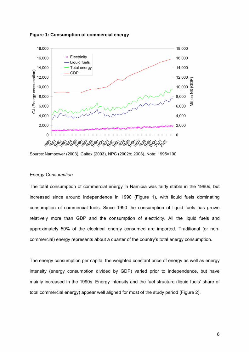
Figure 1: Consumption of commercial energy

0

2,000

4,000

6,000

8,000

10,000

12,000

14,000

16,000

18,000

1980

1981

1982

1983

1984

1985

1986

1987

1988

1989

1990

1991

1992

1993

1994

1995

1996

1997

1998

1999

2000

2001

2002

GJ

(Ene

rgy

cons

umpt

ion)

0

2,000

4,000

6,000

8,000

10,000

12,000

14,000

16,000

18,000

Mill

ion

N$

(GD

P)

ElectricityLiquid fuelsTotal energyGDP

Source: Nampower (2003), Caltex (2003), NPC (2002b; 2003). Note: 1995=100

Energy Consumption

The total consumption of commercial energy in Namibia was fairly stable in the 1980s, but

increased since around independence in 1990 (Figure 1), with liquid fuels dominating

consumption of commercial fuels. Since 1990 the consumption of liquid fuels has grown

relatively more than GDP and the consumption of electricity. All the liquid fuels and

approximately 50% of the electrical energy consumed are imported. Traditional (or non-

commercial) energy represents about a quarter of the country’s total energy consumption.

The energy consumption per capita, the weighted constant price of energy as well as energy

intensity (energy consumption divided by GDP) varied prior to independence, but have

mainly increased in the 1990s. Energy intensity and the fuel structure (liquid fuels’ share of

total commercial energy) appear well aligned for most of the study period (Figure 2).

7

Figure 2: Energy intensity and fuel structure

0.00

0.50

1.00

1.50

2.00

2.50

3.00

1980

1981

1982

1983

1984

1985

1986

1987

1988

1989

1990

1991

1992

1993

1994

1995

1996

1997

1998

1999

2000

2001

2002

MJ/

N$

70

72

74

76

78

80

82

%

Energy intensity (MJ/N$)Liquid fuels as % total energy

Source: NPC (various editions) and Caltex (2003).

Figure 3: Consumption of electricity and maximum demand capacity

50

100

150

200

250

300

350

400

450

1980

1981

1982

1983

1984

1985

1986

1987

1988

1989

1990

1991

1992

1993

1994

1995

1996

1997

1998

1999

2000

2001

2002

GW

h

50

100

150

200

250

300

350

400

450

MW

GWhMW

Source:Nampower(2003).

Consumption of electrical energy has grown less than the maximum demand capacity,

implying a decrease in the average load factor in Namibia (Figure 3). The consumption of

8

electrical energy has grown much in line with the national GDP and contrary to the decrease

in the marginal price for electrical energy.

Figure 4: Diesel and petrol consumption and prices

0

200,000

400,000

600,000

800,000

1,000,000

1,200,000

1,400,000

1,600,000

1,800,000

2,000,000

1980

1981

1982

1983

1984

1985

1986

1987

1988

1989

1990

1991

1992

1993

1994

1995

1996

1997

1998

1999

2000

2001

2002

GJ

0

50

100

150

200

250

300

350

400

450

500

Nc/

l

Diesel consumption (GJ)Petrol consumption (GJ)Diesel price (Nc/l)Petrol price (NC/l)

Source: Caltex (2003), Engen (2002), MME (2002).

The consumption of liquid fuels per capita has increased since independence, and more so

than GDP per capita. The real cost of liquid energy has generally fallen during the study

period. Diesel, followed by petrol, is the dominant liquid fuel in Namibia. The volumes of

kerosene and LPG are relatively negligible. Petrol and diesel consumption are generally

growing, but at different paces. This is possibly a result of differences in use. Petrol is only an

on-shore transport fuel. Diesel is used for automotive purposes (private vehicles, rail and all

types of trucks), offshore vessels and stationary motive power. The real prices of petrol and

diesel are closely related. When in 1999 prices started to rise, diesel consumption continued

to grow while the growth in petrol consumption levelled off (Figure 4).

9

Figure 5: Fuel consumption in peace and war

0

10

20

30

40

50

60

70

80

90

100

1987 1988 1989 1990 1991 1992 1993 1994 1995 1996 1997 1998 1999 2000

Mill

ion

litre

s

Government diesel consumption Jet fuel

Battle of Cuito Canavale Implementation of UN Resolution 435 commences

Independence (March 1990)

Source: Caltex (2003). Note: Data on jet fuel are not available before 1987. Data on government consumption shows that their use of diesel increased steadily from the late seventies until an all-time high in 1988. The battle of Cuito Canavale was a military turning point in the war.

Government’s consumption of diesel, and the overall use of jet fuel, dropped sharply after a

peace accord was reached for Namibia (Figure 5), implying that much of the previous

government’s fuel consumption was related to the war. By independence, energy

consumption reflected, for the first time in many years, the energy demand of a country at

peace and without extensive military activities.

3. Model and data

Our aggregated, long-run energy demand function is specified as follows:

edt= α + β1 yt + β2 pt + β3 xt + µt (1)

10

where edt is the consumption of energy, yt is GDP and pt is the price of energy. Lower case

letters denote log values. We estimate (1) for total national energy consumption and for the

consumption of each type of energy (electricity, petrol and diesel) using non seasonally

adjusted quarterly data for the entire 1980q1 to 2002q4 period as well as for the post-

independence sub-period 1990q1 to 2002q4. In addition to GDP and the price variable, all

our estimated regressions test for the significance of additional regressors (xt), namely, air

temperature, the HIV/AIDS incidence rate and, in the individual energy type equations, also

the price of alternative forms of energy.

Volume data of different energy forms are aggregated using heating values according to the

conversion factors reported in DUKES (UK Digest of Energy Statistics, 2001). When the

consumption of a combination of energy forms is estimated, the relative amount of energy

(expressed in Joules) is multiplied by the marginal price for that energy form in order to arrive

at the weighted marginal energy price.

Nampower’s internal accounting records are the source of data for aggregated consumption

of electricity as well as for marginal and average prices. Nampower’s sales to Local

Authorities are distributed to end-users at prices traditionally set by the individual Local

Authority. We obtained good quality end-user data from the large municipalities. These data

have been extracted from unpublished printed records held by the Municipalities of

Swakopmund, Walvis Bay, Windhoek and Tsumeb. These data represent about 50% of all

electricity consumed in Namibia. To track changes in energy tariffs charged by the Local

Authorities, we have retrieved most of the relevant copies of the Government Gazette from

libraries in Windhoek and Cape Town since the mid 1970s (Government Gazette, 1975 –

2002). The published tariffs include both energy tariffs (marginal prices) and demand

charges. We calculated the weighted marginal cost of electricity for all end-users in Namibia

by combining the tariffs for consumers located in Local Authorities and the weighted

Nampower tariffs for end-user consumer groups.

11

Various petrol companies supply liquid fuels to the Namibian market. Caltex in South Africa

serves as a secretariat for the petrol companies in Namibia and has generously made the

combined sales volumes statistics available to us (Caltex, 2003). The pump-price for a

certain liquid fuel is the same for all consumer groups in the same geographical area. But

diesel consumers in the fisheries, mining, agricultural and construction sectors can apply for

a sector-specific refund (rebate) for part of the road tax component of the pump price. The

marginal price for liquid fuels equals the ‘pump price’, and where applicable, the rebated

pump price for diesel. Post-independence price data were obtained from MME (2002), who

controls the prices for diesel and petrol. BP Namibia (2002) provided LPG price data while

Shell Namibia (2003) provided kerosene prices. The compilation of pre-independence diesel

and petrol prices, and most of the kerosene and LPG prices, was done by going through a

variety of records kept with the South African Petroleum Industry Association (SAPIA, 2002)

and petrol companies in Cape Town (Engen, 2002). Caltex’ volume data do not differentiate

between the different grades of petrol. The prices for the different grades are closely linked.

The correlation coefficient for changes in the prices for Super and Premium grade petrol was

99.66% for the period from 1971 to 1999, and 99.93% for Premium and Regular grade petrol.

We use price data for Premium grade petrol as representative of all octanes of petrol.

Namibia’s GDP per capita is one of the highest in Africa, and its Gini coefficient is one of the

highest in the world. Energy analysis based on consumption per capita when the Gini

coefficient is extreme is of limited relevance at the national level, unless the skew in income

(and energy consumption) distribution is either constant or if the pattern of change is known.

We therefore use total GDP rather than per capita. Quarterly GDP data are only available for

the period from 1993 to the end of 2002 (NPC, 2003). Given the high correlation (95%)

between annual GDP and the Consumer Price Index (CPI) for the period 1980 to 2002, we

used the Friedman (1962) interpolation technique to estimate the quarterly GDP data for the

12

period 1980 to 1993 based on CPI data for the same quarters. The official CPI is published

monthly on the website of the Bank of Namibia.

The HIV/AIDS epidemic is still in its infancy in Namibia but has the potential for devastating

demographic effects. There are no continuous time-series data for the HIV incidence rate in

Namibia. Observations have been recorded by ante-natal clinics, at bi-annual frequencies.

The available time series is short. We have interpolated the existing data (MHSS, 1999;

2000; 2001), and extrapolated back to the time the first incidence was recorded.

The Namibia Meteorological Services (2003) provided daily (mean minimum, mean and

mean maximum) temperature data for certain locations in Namibia. We use temperature data

from Windhoek as a proxy for national weighted average temperature. Windhoek, physically

located in the middle of the country, is also the economic centre of Namibia (about 30% of

the national electrical energy is consumed in Windhoek).

4. Methodology

Before cointegration methods were introduced, the ARDL framework was seen as the most

attractive approach for modeling energy demand relationships since it reflected the pattern

often seen in energy consumption, where sluggish adjustments in demand take time to fully

materialize. However, the advent of cointegration analysis, with its emphasis on retaining the

long-run information in the data by exploiting a cointegrating relationship (if found) among

variables in levels, has come to signify the overt dismissal of the traditional ARDL approach

(Bentzen and Engsted, 2001).

Although the Johansen (1988) method is by no means the only approach to cointegration, it

has enjoyed widespread adoption since its inception. The most obvious advantage of the

Johansen method is that it allows estimation of multiple cointegrating vectors where they

exist. Far too often, however, practitioners fail to recognize that the application of the

13

Johansen technique presupposes that the underlying regressors are all integrated of order

one (Pesaran et al., 2001). This is necessary because in the presence of a mixture of

stationary series and series containing a unit root, standard statistical inference based on

conventional likelihood ratio tests is no longer valid. Harris (1995), for example, notes that

the trace and maximum eigenvalue tests from the Johansen procedure may lead to

erroneous inferences when I(0) variables are present in the system since stationary series

are likely to generate spurious cointegrating relations with other variables in the model.

Significantly, Pesaran and Shin (1999) and Pesaran et al. (2001) developed a new ARDL

bounds testing approach for testing the existence of a cointegration relationship that is

applicable irrespective of whether the underlying series are I(0), I(1). This approach,

therefore, rehabilitates the ARDL framework while overcoming the problems associated with

the presence of a mixture of I(0) and I(1) regressors in a Johansen-type framework.

To implement this technique, we start by modelling equation (1) as a conditional ARDL-ECM:

tttttt

p

k

q

rrtrktkjt

n

jj

m

iiti

xpyedD

xpyxtccedt

ξππππϕ

φδβα

++++++

∆+∆+∆+∆++=∆

−−−−

= =−−−

==− ∑ ∑∑∑

14131211

0 00110 (2)

where c0 and c1 t are the intercept and time trend components. Despite its restrictive nature,

the latter is included to capture the effect of technical progress and other exogenous impacts

that are not measurable directly (see Hunt et al., 2003, for further discussion). Dt is a vector

of dummy variables included to allow for significant trend or level breaks (due to shocks in

prices or impacts related to the transition to independence) or pulses in the series (due to

outlier observations). The different types of dummies are explained through their notations,

and their significance reported in Tables 3 to 8. The dummy notation starts with the letter ‘D’

and is followed by three digits (XXX) referring to the year and the quarter. The last letter of

the dummy shows whether it refers to a trend break (TB), shift of level (L) or a pulse (P). Tc

14

represents the quarter when the trend break, level shift or pulse took place. t is the time axis.

DXXXL = 1 if t ≥ Tc and = 0 if t < Tc ; DXXXTB = t – Tc-1 if t ≥ Tc and = 0 if t < Tc; DXXXP = 1

if t = Tc, and = 0 otherwise.

ξt are assumed to be white noise error processes. The lag structure of the first difference

regressors is set to ensure an absence of serial correlation in the estimated residuals. We

report the order of the chosen ARDL process guided by the Schwarz Criterion (SC) for each

estimated equation in Tables 3 to 8.

Following Pesaran et al., (2001), we regard yt, pt and xt as ‘long-run forcing’ variables for edt,

in the sense that there is no feedback from the level of edt in (2). This assumption implies

weak exogeneity of the regressors, i.e. that the explanatory variables are not cointegrated

among themselves and that, therefore, the cointegrating rank (i.e. the number of

cointegrating vectors) is restricted to unity.

It should be emphasised at this point that in implementing this methodology, OLS estimation

of the ARDL-ECM (run using the Microfit 4 software package, see Pesaran and Pesaran,

1997) is merely an intermediate step necessary to undertake the bounds tests for

cointegration. Equation (2), therefore, is not aimed at the estimation of short-run elasticities,

which go beyond the scope of this paper.

The null hypothesis of ‘no cointegration’ is tested using an F-statistic for the joint significance

of the coefficients of the lagged levels in (2). Pesaran et al. (2001) prove that, under the null

hypothesis, the asymptotic distribution of the F-statistic is non standard irrespective of

whether the regressors are I(0) or I(1), and provide two adjusted critical values that constitute

upper and lower bounds of significance. If the F statistic exceeds the upper critical value we

can conclude that a long-run relationship exists. If the F statistic falls below the lower critical

value we cannot reject the null hypothesis of ‘no cointegration’. If the statistic lies within the

15

respective bounds, inference would be inconclusive. Critical values are also made available

to encompass a range of different drift and trend components.

Should a cointegrating relationship be found, the next step in implementing this methodology

is to estimate the conditional long-run model for edt, which can be obtained from the reduced

form solution of (2), when ∆ed=∆y=∆p=∆x=0:

tttt xpytedt ν+Θ+Θ+Θ+Θ+Θ= 54321 (3)

where Θ1= -c0/π1, Θ2= -c1/π1, Θ3= -π2/π1, Θ4= -π3/π1, Θ5= -π4/π1, and νt is an IID (0,σ2) error

process. These long-run coefficients, which form the focus of our empirical analysis, are

those reported in Tables 3 to 8.

6. Estimation results

While the ARDL bounds testing approach to cointegration allows regressors to be either I(0)

or I(1), it is still necessary to ensure that the dependent variable is I(1) in levels and that none

of the regressors is I(2) or higher. Accordingly, all variables were tested for unit root (UR). UR

testing was performed using Dickey-Fuller (DF) or Augmented Dickey-Fuller (ADF) tests for

series that did not display any apparent structural breaks. Since Perron (1989) demonstrated

that the ADF tests cannot reject the null hypothesis of a unit root against trend stationary

alternatives if the data generating process is one of stationary fluctuations around a trend

function with a one-time break, when visual inspection of the time series indicated a single

break point we employed the Perron (1989) UR test. Perron (1989) calculated critical values

for the autoregressive coefficient α~ in equation (4), for each of three cases which allow for an

exogenous break, at time t, in level, in rate of growth and in both level and rate of growth.

The critical values also account for alternative λs (with 10% intervals), where λ is a measure

of how far into the sample the break took place.

ttt yty εαβµ ~~~~1 +++= − (4)

16

The detailing of Perron’s (1989) test is beyond our scope, suffice to say that if the estimated

α~ in our UR testing of variables where one break is suspected is less than Perron’s critical

value (in absolute terms), the null hypothesis of a unit root is not rejected.

In the case of two structural break points, we employed the Lumdsaine and Papell (1997) UR

model given in (5):

∑=

−− +∆+++++++=∆k

itititttttt ycyDTDUDTDUty

112211 εαψωγθβµ (5)

where DU1t and DU2t are dummies for a mean shift occuring at times TB1 and TB2. DT1t

and DT2t are dummies for the corresponding trend-shifts. DU1t = 1 if t>TB1, DU2t = 1 if

t>TB2, DT1t = (t-TB1)1 if t > TB1, and DT2t = (t-TB2)1 if t > TB2. t = 1,…..,T. UR testing is

done by comparing the relevant estimated values from (5) with the relevant critical values

provided by Lumsdaine and Papell (1997).

The results of our UR testing are shown in Table 2. As a matter of interest, Table 2 also

reports the standard (A)DF test statistics and associated critical values in the cases in which

the UR test was done according to the Perron (P) or Lumsdaine and Papell (LP) tests. We

found that all dependent variables used in our estimations were I(1). With respect to the

regressors, GDP and air temperature were found to be I(0) while all other regressors

contained a unit root in levels. The finding of a mixture of I(1) and I(0) regressors is

particularly important to appreciate the merit of this methodology in that it confirms the use of

the ARDL bounds testing approach to cointegration as the most appropriate and reliable

estimation technique given the time series properties of our data.

TABLE 2 HERE

The results of the bounds testing (and the order of the ARDL processes) are reported for

each estimated regression in Tables 3 to 8. Since in all cases the computed bounds (F)

statistic is greater than the upper critical value, these tests confirm the existence of a

cointegrating relationship between the dependent variable and the regressors within each of

17

the estimated equations. Armed with this finding, we next proceed to build on it by estimating

the long-run models. Tables 3 to 8 also report several diagnostic tests, all of which suggest

an adequate model specification and high goodness of fit of the individual equations (for

more details see the Note at the bottom of Table 3).

TABLE 3 HERE

Table 3 reports the results of the estimation of the national consumption of all commercial

energies as a function of weighted total energy price, GDP, temperature and the dummy

D884L. All regressors are highly significant. National energy consumption appears to be

income elastic, price inelastic and sensitive to mean minimum temperature. Energy

consumption increases (or decreases) when temperature decreases (or increases). The

trend and level of the weighted marginal national energy price changed various times during

the sample period. Only the break in 2001q2 is significant, and then only in the bounds test

for the post-independence period. The HIV incidence rate was insignificant as an

explanatory variable and was therefore omitted from the preferred equation. The long-run

elasticities for price, GDP and temperature for the 1990q1 to 2002q4 period and the period

1980q1 to 2002q4 are similar. This implies that D884L sufficiently captures structural

changes around the time of independence.

TABLE 4 HERE

Table 4 shows that the significant explanatory variables for the total consumption of grid

electricity in Namibia are the price of electricity, GDP and mean minimum temperature.

When a low temperature gets even lower (or higher), more (or less) electrical energy is

consumed in Namibia. Changes in high temperatures do not normally have the same effect.

The long-run GDP elasticity is about twice the absolute value of the long-run price elasticity.

Diesel and kerosene prices were found to be insignificant. There are in other words no

cross-price elasticities between electricity, diesel and kerosene.

Electricity from the public grid could, in principle, be regarded as a potential alternative to

diesel and kerosene for the provision of various energy services. A consumer can, in

18

principle, choose to run a diesel auto-generator instead of drawing electricity from the grid.

Similarly, a household can choose to use kerosene lamps rather than electric bulbs. The

absence of significant cross-price elasticities between diesel and electricity is probably due

to the fact that the opportunity to switch between grid electricity and auto-generators is

limited in areas outside the municipalities. Where grid electricity is made available outside

municipal areas, farmers and companies do connect as they find grid power more reliable

than operating auto-generators. Auto-generators might then be kept for fall-back purposes, if

the grid supply were to be interrupted, but would in general not be used in an on/off fashion

depending on variations in the relative price between diesel and public electricity.

The amount of energy relevant for switching between grid electricity and kerosene for

lighting purposes as a result of variations in relative prices can only be marginal. The amount

of kerosene sold in Namibia during the last five years (litres converted to Joules = heating

values) is only 6.26% of the electricity consumed in the country (KWh converted to Joules).

The government of independent Namibia has pursued an active policy of making electricity

available in rural areas and to consumers that were deprived of this energy form during the

colonial dispensation. One might intuitively expect the implementation of this policy to be

reflected in a positive and significant time-trend in the estimation of the national consumption

of electricity. This is in fact not the case. The amount of electricity sold to rural areas,

although growing strongly, is small compared to consumption in urban areas. Hence, the

growth in rural electricity consumption does not have a major impact on national

consumption. The associated time-trend is not significant. The dummy reflecting

independence (INDDUM) was not significant.

As noted earlier in the paper, one can estimate national energy consumption per capita, or

include the size of the population as a regressor. We found that the high correlation (96.1)

between total population and national GDP caused multicollinearity problems. For the sake

19

of completeness, therefore, we also estimated a model of electricity consumption per capita

and found that the long-run elasticities were lower in the per capita case. This points to the

possible role of the growing size of the population as an explanatory variable for the

increased electricity consumption over time. But this cannot be proven without better data on

the rate of electrification (the proportion of the population actually connected to the electricity

grid) and the rate of change (if any) in income distribution. In Namibia, with so many people

living in subsistence economies, electricity or energy consumption per capita is possibly

nothing but a statistical concept with little relevance for meaningful demand analysis at the

national level. The 2R for the estimate of the electricity consumption per capita was much

lower (0.55) than the 2R for the aggregated electricity consumption (0.97). The regressors

were also less significant in the per capita model. For these reasons, the model for

aggregated national electricity consumption (Table 4) is our preferred model.

TABLE 5 HERE

As shown in Table 5, the consumption of petrol is found to be price and GDP elastic, but less

sensitive to temperature fluctuations. Comparing estimations for the entire period with the

post-independence period shows that the significant regressors are the same, with only

minor differences in their values. This supports that INDDUM picks up the effect on petrol

consumption of the transition from pre- to post-independence.

The high correlation between petrol and diesel prices creates problems of multicollinearity. It

is not possible to distinguish any effect on petrol consumption as a result of changes in

diesel prices. The same holds for the consumption of transport diesel as a function of petrol

prices. Unfortunately, sufficient data were not available for other potentially important

variables, such as the price indices for petrol and diesel vehicles, or the extent of the tarred

roads network. However, the good diagnostic results imply that the model adequately

estimates the demand for petrol in Namibia. Petrol is a transport fuel, and is not a substitute

20

to (or from), or complementary with, electricity and kerosene. The estimations found that the

prices for electricity and kerosene were not significant for the consumption of petrol.

Diesel was a major fuel for the war machine prior to independence, and we expected this to

influence the estimation of the diesel consumption for the entire period 1980q1 to 2002q4.

As shown in Table 6, the estimate for the diesel price elasticity has the expected sign but is

not significant. The mean maximum temperature variable was more significant than the

mean minimum temperature. When the low and the high temperatures were combined in the

same equation the mean minimum temperature was insignificant.

TABLES 6 & 7 HERE

As discussed earlier, a government policy is to refund part of the fuel tax to certain

consumers when their diesel consumption is related to non-transport purposes. We modelled

diesel consumption using the calculated weighted rebated diesel price, and, as an

alternative, the non-rebated pump price (Table 6). The resulting estimates were almost

identical and the price elasticity was insignificant in either case. The national weighted

rebated diesel price includes a large amount of non-rebated diesel (two thirds of total

consumption). The fact that neither the rebated nor the pump price is statistically significant

does not say anything about the effect of the rebate in the respective economic sectors.

Whether the rebate is important or not must be analyzed at the sectoral level. Table 7 shows

the estimated regression after the price variable was dropped.

Petrol is exclusively a transport fuel, while diesel is a multi-purpose fuel. Transport diesel is

used in all sectors, and is the dominant fuel for heavy goods and commodity transport in

addition to buses and trains. Petrol is the main fuel for private cars and smaller vans. The

national demand for petrol and diesel therefore respond differently to changes in price, GDP

and temperature variables.

TABLE 8 HERE

21

In Table 8 we limit estimation of diesel consumption to the post-independence period. The

value of the long-run GDP elasticity changes marginally, diesel price is still insignificant, and

the long-run elasticity for temperature is reduced. The peaceful post-independence situation

presents a different consumption pattern for diesel but despite this, the GDP elasticity does

not change much when the 1990q1-2002q4 period is estimated.

6. Discussion

The difference in elasticities for the various energies reflects the difference in services

provided by the various fuels. There are no significant cross-price elasticities for the various

energy forms. The lower 2R for diesel consumption probably reflects the fact that diesel has

a more diverse utilization than other fuels.

Our focus in this paper was on long-run elasticities. Our estimates of aggregated energy

consumption compare well with those per capita figures reported by Pesaran et al. (1998),

who also employed the ARDL bounds testing approach to cointegration. They found a mean

long-run income elasticity of 1.23 and a mean long-run price elasticity of –0.261. Our figures

for total energy consumption are 1.27 and –0.34 but we were able to control for temperature

as an exogenous variable. There are major variations among the 10 Asian countries studied

by Pesaran et al. (1998). Our income and price elasticities are closest to those of Thailand;

1.17 and –0.34 respectively. Both Namibia and Thailand are low middle income countries.

In her survey Dahl (1994) reports income elasticities of 0.69 to 1.68, and price elasticities of

-0.30 to –0.96 for the sub-Saharan region for alternative periods from 1960 to 1975. For the

period from 1970 to 1980 she reports an intermediate income elasticity of 1.28 and price

elasticity of –0.94 for Botswana, and 1.33 and -0.97, respectively, for Nigeria.

We found different price, GDP and temperature elasticities for the consumption of various

energy forms. Diesel has the highest long-run GDP and temperature elasticities (in absolute

22

values) (1.96 and –1.12 respectively). Petroleum has the highest long-run price elasticity (-

0.86), while electricity’s is lower (-0.30). Electricity has the lowest long-run GDP elasticity

(0.59), while petroleum’s (1.08) is between those of diesel and electricity.

Balabanoff (1994) reports income and price elasticities for electricity from South America

from the 1970s to the early 1990s. The estimates for Brazil were 1.73 and –0.43, and for

Columbia 1.88 and –0.18 respectively. Brenton (1997) found an expenditure elasticity for

electricity of 1 for middle income countries, and a price elasticity of –0.69. Electricity prices in

Namibia were for many years the lowest in the world. This could hinder the relevance of a

direct comparison of Namibian electricity elasticities with those from other continents.

Our estimated results for the consumption of electricity are in direct contradiction to those of

Lundmark (2001), who applied simple OLS in regressing Namibian electricity demand on

electricity and coal prices, and on GDP. He used annual data for the period 1980 to 1996.

None of his coefficients were significant, and the regression’s 2R was 0.789. The

comparison acts as a reminder of the need to apply appropriate data (he did not compile

end-user prices), to use a correct model (his coal prices are not relevant for the end-use of

electricity in Namibia), to employ a large sample (his estimation was only based on 17

observations), and a suitable methodology (Lundmark did not deal with the time-series

properties of the series).

A number of researchers (Sailor and Munoz, 1996; Al-Faris and Ghali, 1998; etc.) have

found that climatic variables play a significant role in the demand for energy. None of these

studies, however, relate to energy consumption in Africa. Low temperatures are in general

significant in our models for Namibia, while the significance of high temperatures is limited to

diesel consumption. This confirms that much of the commercial energy in Namibia is used for

producing heating rather than cooling services. Heating services are cheaper and more

accessible. Variations in low temperatures affect energy demand more than variations in high

23

temperatures. The lack of symmetry between the heating and cooling services also highlights

the difference between the energy demand function of Namibia vis-à-vis that of an OECD

country, where there is also high saturation of cooling appliances.

Our findings appear to have significant policy implications, particularly with respect to the

way in which taxation could help the Namibian government increase fiscal revenues and

regulate the level and/or structure of energy consumption. For example, if government

needed to increase its tax revenues, comparatively more tax could be charged on diesel than

on petrol since we found the price elasticity for diesel to be much lower than for petrol. It is in

practice difficult to have different energy taxes for all consumer groups as government may

not be able to control their sourcing of liquid fuels. One method used in certain European

countries is to mix different coloring agents into the diesel to be sold at different taxation

levels. This method has not been tried in Namibia and could prove useful for more selective

energy taxation and pricing. Additionally, the differences in price elasticities across fuels

uncovered by our empirical analysis provide valuable evidence for informing environmentally

motivated energy taxation, should the Namibian government wish to pursue this as a policy

objective.

7. Conclusions

In this paper we presented the first econometric study of Namibian energy demand at

aggregated level and by energy type, that uses high quality, quarterly end-user data covering

a relatively long period (1980-2002). Our results have shown that energy demand in Namibia

conforms to a priori expectations of a negative price elasticity and a positive GDP elasticity.

In most cases we also find a negative temperature elasticity.

Diesel has the highest GDP and temperature elasticities (in absolute terms). The price

elasticity for the consumption of petrol is much higher than that of electricity (in absolute

terms), while diesel does not display any significant price elasticity. The differences in price

24

elasticities across fuel types have clear implications for energy taxation by Namibian policy

makers. The consumption of electricity has the lowest GDP elasticity, while the GDP

elasticity for the consumption of petrol is between that of electricity and diesel.

We did not find any significant cross price elasticities between different energy forms.

Consumers appear to retain their fuel mix and consumption level. They seem to get ‘locked’

into a set of appliances and equipment for the provision of the energy services they require,

and do not easily break away from that pattern even if prices and income change.

Additionally, our results have also shown that the relatively recent but very high HIV

incidence rate in Namibia has not yet made its mark on energy consumption.

Notwithstanding the value of our findings, it should be borne in mind that energy demand

might assume different connotations in different economic sectors. Sectoral consumers do

not make optimal demand decisions under the same constraints and do not necessarily

demand the same services from the various energy forms. A sectoral analysis of the

Namibian demand for energy, therefore, offers a profitable avenue for future research.

25

References

Al-Faris, A.F. and Ghali, K.H., 1998. Environment-based forecasting of peak-load profiles for electricity consumption in the western United Arab Emirates. The Journal of Energy and Development 24 1, 1-15. Balabanoff, S., 1994. The dynamics of energy demand in Latin America. OPEC Review Winter, 467-488. Bentzen, J. and Engsted, T., 2001. A revival of the autoregressive distributed lag model in estimating energy demand relationships. Energy 26, 45-55. BP Namibia (2002). Namibian LPG prices. Unpublished database. BP Namibia. Windhoek. Brenton, P., 1997. Estimates of the demand for energy using cross-country consumption data. Applied Economics 29, 851-859. Caltex, 2003. Sales volumes of liquid fuels in Namibia 1979-2002. Unpublished database. Caltex, Cape Town. Dahl, C., 1994. A survey of energy demand elasticities for the developing world. The Journal of Energy and Development 17 1, 1- 47. DUKES (2001) UK Digest of Energy Statistics 2001. DTI, London. Edmonds, J. and Reilly, J.M., 1985. Global Energy: Assessing the Future. Oxford University Press, Oxford. Engen, 2002. Various sales data for petroleum, diesel and kerosene. Unpublished company records. Engen, Cape Town. Engle, R. and Granger, C., 1987. Co-integration and error correction: representation, estimation and testing. Econometrica 55 2, 251-276. Friedman, M., 1962. The interpolation of time series by related series. Journal of the American Statistical Association 57 December, 729-757. Gately, D. and Huntington, H.G., 2002. The asymmetric effects of change in price and income on energy and oil demand. Energy Journal 23 1, 19-55. Government Gazette (1975-2002). Government of the Republic of Namibia, Windhoek. Griffin, J.M. and Schulman, C.T., 2005. Price asymmetry in energy demand models: A proxy for energy-saving technical change? The Energy Journal 26 2, 1-21. Harris, R., 1995. Using Cointegration Analysis in Econometric Modelling. Prentice Hall, London. Hunt, L.C., Salgado, C. and Thorpe, A., 2000. The policy of power and the power of policy: Energy policy in Honduras. The Journal of Energy and Development 25 1, 1-36. Hunt, L.C., Judge, G. and Ninomiya, Y., 2003. ‘Modelling underlying energy demand trends’. Chapter 9 in L.C. Hunt (Ed.) Energy in a Competitive Market: Essays in Honour of Colin Robinson, Edward Elgar, May, pp. 140-174.

26

IEA, 2002. Key World Energy Statistics (2001 Edition). IEA, Paris. Ibrahim, I.B. and Hurst, C., 1990. Estimating energy and oil demand functions – A study of thirteen developing countries. Energy Economics 12, 93-101. Johansen, S., 1988. Statistical analysis of cointegration vectors. Journal of Economic Dynamics and Control 12, 231 –254. Johansen, S., 1991. Estimating and hypothesis testing of cointegration vectors in Gaussian vector autoregressive models. Econometrica 59 6, 1551-1580. Levine, M.D., Koomey, J.G., Price, L., Geller, G. and Nadel, S., 1995. Electricity end-use efficiencies: Experience with technologies, markets, and policies throughout the world. Energy 20 1, 37-61. Lumsdaine, R. and Papell, D., 1997. Multiple trend breaks and the unit-root hypothesis. Review of Economics and Statistics 19, 212-218. Lundmark, R., 2001. Changes in Namibia’s energy market. Scandinavian Journal of Development Alternatives and Area Studies 20 1-2, 103-112. MHSS, 1999. Report of the HIV Sentinel Sero Survey. Ministry of Health and Social Services, Windhoek. MHSS, 2000. Projecting the impact of HIV/AIDS in Namibia. Ministry of Health and Social Services, Windhoek. MHSS, 2001. Report of the HIV Sentinel Sero Survey. Ministry of Health and Social Services, Windhoek. MME, 1998. White Paper on Energy Policy. Ministry of Mines and Energy, Windhoek. MME, 2000. Electricity Act. Act 2 of 2000. Ministry of Mines and Energy, Windhoek. MME (2002) Controlled prices for Petrol and Diesel 1989-2002. Unpublished data files from the Ministry of Mines and Energy, Windhoek. Namibia Meteorological Services, 2003. Monthly temperature data for selected locations in Namibia. Unpublished. Ministry of Works, Transport and Communication, Windhoek. Nampower, 2003. Various internal sales and accounting data. Nampower, Windhoek. NPC, 1995. First National Development Plan (NDP 1) – Volume 1 – 1995/1996-1999/2000. National Planning Commission, Windhoek. NPC, 2002a. Volume 1: Macroeconomic, sectoral and cross-sectoral policies. Second National Development Plan – (NDP2). National Planning Commission, Windhoek. NPC, 2002b. National accounts 1980 – 2001. National Planning Commission, Windhoek. NPC, 2003. National Accounts 1994 – 2002. National Planning Commission, Windhoek. Perron, P., 1989. The great crash, the oil price shock, and the unit root hypothesis. Econometrica 57, 1361-1401. Pesaran, M.H. and Pesaran, B., 1997. Microfit 4.0. Oxford University Press, Oxford.

27

Pesaran, M.H., and Shin, Y., 1999. An autoregressive distributed-lag modelling approach to cointegration analysis, in: Strøm, S. (Ed.) Econometrics and Economic Theory in the 20th Century. Cambridge University Press, Cambridge. Pesaran, M.H., Smith, R. and Akiyama, T., 1998. Energy demand in Asian economies. Oxford University Press, Oxford. Pesaran, M.H., Shin, Y. and Smith, R.J., 2001. Bounds testing approaches to the analysis of level relationships. Journal of Applied Econometrics 16, 289-326. Pourgerami, A. and von Hirschhausen, C.R., 1991. Aggregate demand for energy and dynamics of energy elasticities in non-oil developing countries. The Journal of Energy and Development 14 2, 237-252. Sailor, D. and Munoz, R.J., 1996. Sensitivity of electricity and natural gas consumption to climate in the USA - methodology and results for eight states. Energy 22 10, 987-998. SAPIA, 2002. Price increases for petrol, diesel and kerosene. Unpublished data files. The South African Petroleum Industry Association, Cape Town. Shell Namibia, 2003. Paraffin prices in Grootfontein, Windhoek and Walvis Bay 1999-2002. Shell Namibia, Windhoek. Stage, J., 2002. Structural shifts in Namibian Energy Use: An input-output approach. The South African Journal of Economics 70 6, 1103-1125. Stage, J. and Fleermuys, F., 2001. Energy use in the Namibian economy from 1995 to 1998. Development Southern Africa 18 5, 423-441. Woodland, A.D., 1993. A micro-econometric analysis of the industrial demand for energy in New South Wales. Energy Journal 14 2, 57-89.

28

Table 1: Summary of elasticities from main studies on developing countries Long-run Short-run Country Period

Dep

ende

nt

varia

ble

(dem

and

for:

)

GD

P

(Inco

me)

Pric

e

Oth

er

GD

P

(Inco

me)

Pric

e

Sour

ce

Bangladesh 1.98 0.04 India 1.01 -0.07 Indonesia 1.56 -0.49 Korea 1.07 -0.14 Malaysia 2.21 -1.16 Pakistan 1.32 0.05 Philippines 0.84 -0.43 Sri Lanka 0.22 0.06 Taiwan 0.90 -0.13 Thailand 1.17 -0.34 Mean

19

73-1

990

E

nerg

y

1.23 .-0.26 Bangladesh 1.625 0.000 India 0.436 -0.033 Indonesia 1.286 -0.324 Korea 1.387 -0.203 Malaysia 3.318 -1.753 Pakistan 1.425 0.165 Philippines 1.187 -1.324 Sri Lanka 0.578 0.101 Taiwan 1.038 -0.005 Thailand 1.474 -0.375 Mean group estimate

19

73-1

990

Tr

ansp

ort s

ecto

r ene

rgy

1.375 -0.375

Bangladesh 1.252 -0.043 India 1.643 -0.005 Indonesia 1.187 -0.569 Korea 0.624 0.203 Malaysia 1.004 -0.286 Pakistan 2.947 -0.334 Philippines 1.654 -0.347 Sri Lanka 0.376 -0.363 Taiwan 0.811 -0.191 Thailand 1.629 -0.114 Mean group estimate

19

73-1

990

R

esid

entia

l ene

rgy

1.312 -0.135

Pes

aran

et a

l. (1

998)

Argentina Oil 1.98 -0.25 Argentina 1.00 n/a Brazil 1.73 -0.43 Chile 1.65 n/a Colombia 1.88 -0.18 Equador 1.95 n/a Peru

19

70-1

990

El

ectri

city

0.70 n/a

Bal

aban

off

(199

4)

Brazil 1.16 -0.15 India 1.56 n/a Morocco 1.03 n/a Phillipines 1.14 -0.17 Taiwan 1.24 -0.24 Algeria 0.89 -0.89 Egypt 0.85 -0.27 Indonesia

19

70s

– ea

rly

1980

s

Ene

rgy

1.19 n/a Ibra

him

and

Hur

st

(199

0)

29

Mexico 1.27 -0.12 Saudi Arabia 1.23 -0.24 Poor countries

-0.073 0.919(i)

Middle-income countries

-0.695 1.007(i)

Rich countries Dat

a co

llect

ed

in 1

980,

for 5

ye

ar in

terv

als

El

ectri

city

-0.704 0.877(i)

Bre

nton

(1

997)

(ii)

sub-Saharan Africa

1960-1975

1.67(iii)

-0.58(iii)

1.67 -0.06

Botswana 1.28(iii)

-0.94(iii)

Nigeria

1970-1980 1.33

(iii)-0.97

(iii)

Average of 50 developing countries

Ene

rgy

1.27 -0.33 0.53 -0.33 Dah

l (19

94)

Brazil 1.0 Colombia 0.8 Mexico 1.2 Venezuela 1.6 All LDCs

1970-1973

1.2 Brazil 1.1 Colombia 0.7 Mexico 2.0 Venezuela 0.5 All LDCs

1973-1978

E

nerg

y

1.4

Edm

onds

and

Rei

lly

(198

5)

Namibia 1980- 1996

Electricity -0.512(iv)

-0.863

Lund

mar

k (2

001)

Electricity 0.786 Honduras 1973- 1995 Petroleum 1.578

Hun

t et a

l. (2

000)

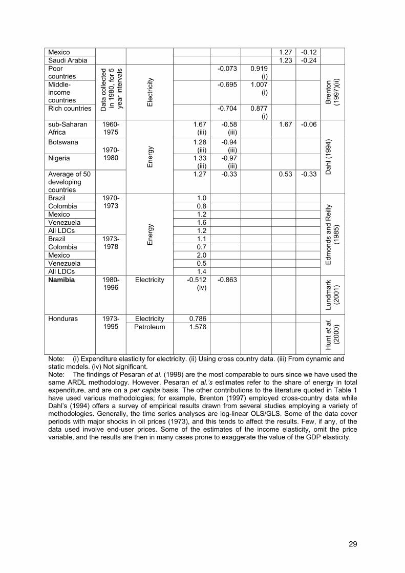
Note: (i) Expenditure elasticity for electricity. (ii) Using cross country data. (iii) From dynamic and static models. (iv) Not significant. Note: The findings of Pesaran et al. (1998) are the most comparable to ours since we have used the same ARDL methodology. However, Pesaran et al.’s estimates refer to the share of energy in total expenditure, and are on a per capita basis. The other contributions to the literature quoted in Table 1 have used various methodologies; for example, Brenton (1997) employed cross-country data while Dahl’s (1994) offers a survey of empirical results drawn from several studies employing a variety of methodologies. Generally, the time series analyses are log-linear OLS/GLS. Some of the data cover periods with major shocks in oil prices (1973), and this tends to affect the results. Few, if any, of the data used involve end-user prices. Some of the estimates of the income elasticity, omit the price variable, and the results are then in many cases prone to exaggerate the value of the GDP elasticity.

30

Table 2: Summary of UR testing

Level Variable

Test(*) Statistic Critical Value

Conclusion

National electricity consumption

ADF -3.326 -3.465 The variable is I(1)

National petrol consumption

ADF P

-2.3982.823

-3.463-4.04

The variable is I(1)

National diesel consumption

ADF P

-1.9560.639

-3.460-3.96

The variable is I(1)

National energy consumption

P ADF

3.6-2.787

3.74-3.464

The variable is I(1)

National marginal (weighted) electricity price

P ADF

-2.964-2.862

-4.17-3.467

The variable is I(1)

Diesel price P ADF

-2.0651.177

-3.99-3.482

The variable is I(1)

Rebated, national diesel price

ADF P

-1.8220.049

-3.461-3.8

The variable is I(1)

Petrol price LP ADF

-6.2940.803

-6.65-3.48

The variable is I(1)

Weighted national energy price

DF P

-2.1313.405

-3.467-4.04

The variable is I(1)

Rebated, national weighted energy price

DF -1.915 -3.461 The variable is I(1)

GDP P ADF

-5.083-3.545

-4.22-3.467

The variable is I(0)

Mean minimum temperature

ADF -4.048 -3.502a The variable is I(0)

Mean maximum temperature

ADF -1.805 -2.895 The variable is I(1)

Note: Unless otherwise stated, the critical values refer to the 95% significance level. Superscript a refers to the 99% level. (*) DF = Dickey-Fuller test. ADF = Augmented Dickey Fuller test. P = Perron’s test. LP = Lumsdaine and Papell’s test.

31

Table 3: National consumption of commercial energy Dependent variable: National energy consumption

1980Q1 – 2002Q4 1990Q1 – 2002Q4 Regressors: Estimate: T-ratio (Prob): Estimate: T-ratio

(Prob): Weighted national energy price

-0.344 -1.992 (0.050) -0.297 -1.985 (0.054)

Total GDP 1.266 5.596 (0.000) 1.286 9.228 (0.000)

Mean minimum temperature

-0.676 -2.696 (0.009) -0.240 -2.205 (0.034)

D012L 0.065 0.921 (0.363)

Intercept 8.802 3.580 (0.001) 6.739 3.148 (0.003)

Long

-run

ela

stic

ities

D884L -0.307 -2.614 (0.011) SEE 0.039 0.036

2R 0.962 0.956 DW-statistic 2.267 2.289 Serial correlation(χ4) 7.475 (0.130) 2.329 (0.675) Functional form(χ1) 1.020 (0.313) 0.857 (0.355) Normality(χ2) 1.425 (0.490) 0.259 (0.879)

Test

s an

d di

agno

stic

s

Heteroscedasticity (χ1) 0.598 (0.439) 1.874 (0.171) Order of the ARDL process (2,0,0,0) (1,0,0,0)

Bounds F statistic vs upper critical value

F 6.218 > 4.855 F 6.353 > 6.309a

Note: For Tables 3 to 8, the critical values of the bounds tests are taken from Pesaran and Pesaran (1997), Table F, p.478. Unless otherwise stated, all critical values refer to the 95% significance level. Where present, the superscript a denotes significance at the 99% level.

Note: For Tables 3 to 8, we also report the following statistics and diagnostic tests. SEE refers to

the Standard Error while 2R expresses the ratio of the explained sum of squares to the total

sum of squares (adjusted for degrees of freedom). Both are ‘goodness of fit’ measures, where SEE should be as small as possible and the 2R as close to unity as possible. The DW statistic refers to the Durbin Watson 0<d>4 test for serial correlation. As rule of thumb, if the statistic d is found to be around 2, one may assume that there is no first-order autocorrelation. Serial correlation refers to the Lagrange multiplier statistic, which specifically tests whether the disturbances are autocorrelated up to order 4. Functional form shows the result of Ramsey’s RESET test using the square of the fitted values. Normality shows the results of the testing of skewness and kurtosis of the residuals while Heteroscedasticity refers to the regression of squared residuals on squared fitted values to establish whether the disturbances have a constant variance. A ‘chi-square’ ( 2χ ) statistic is shown for each of the test statistics and the comparison with the critical values decides whether the regression passes the tests. The order is given in the notation p of pχ . At the 95% level of significance, the critical value is 3.84 for p = 1; 5.99 for p = 2, and 9.49 for p = 4. The number in brackets next to the individual chi-square statistic shows within what percentage of the distribution the individual statistic is found.

32

Table 4: National electricity consumption Dependent variable: National electricity consumption (1980q1-2002q4)

Regressors: Estimate: T-ratio (Prob): Weighted national marginal electricity price

-0.298 -3.042 (0.003)

Total GDP 0.589 5.160 (0.000)

Mean minimum temperature -0.356 -1.966 (0.053)

Long-run elasticities

Intercept 12.031 6.295 (0.000) SEE 0.034

2R 0.971 DW-statistic 1.784 Serial correlation(χ4) 4.493 (0.343) Functional form(χ1) 0.920 (0.338) Normality(χ2) 0.008 (0.996)

Tests and diagnostics

Heteroscedasticity(χ1) 2.191 (0.139) Order of the ARDL process (4,0,1,0) Bounds F statistic vs upper critical value F 5.881 > 4.855

33

Table 5: National consumption of petrol Dependent variable: National petrol consumption

1980q1 – 2002q4 1990q1 -2002q4 Regressors: Estimate: T-ratio

(Prob):Estimate:

T-ratio (Prob)

Petrol price -0.858 -3.803 (0.000)

-0.794

-2.441 (0.019)

Total GDP 1.081 5.786 (0.000)

0.957 7.474 (0.000)

Mean minimum temperature

-0.272 -1.909 (0.061)

-0.199

-1.650 (0.107)

Intercept 12.846 4.630 (0.000)

12.933 3.890 (0.000)

Long

-run

ela

stic

ities

INDDUM -0.311 -2.718 (0.008)

SEE 0.035 0.030 2R 0.978 0.952

DW-statistic 2.192 2.562 Serial correlation(χ4) 8.936 (0.063) 9.755 (0.045) Functional form(χ1) 0.338 (0.561) 0.262 (0.609) Normality(χ2) 1.249 (0.535) 1.386 (0.500)

Test

s an

d di

agno

stic

s

Heteroscedasticity(χ1) 0.477 (0.490) 6.270 (0.012) Order of the ARDL process (8,2,1,0) Bounds F statistic vs upper critical value

F 7.189 > 6.309a

Note: INDDUM = 1 for the period from 1980q1 to 1989q4, and = 0 otherwise.

34

Table 6: National consumption of diesel Dependent variable: National diesel consumption (1980q1-2002q4)

Rebated price Pump price Regressors: Estimate: T-ratio

(Prob):Estimate: T-ratio

(Prob): Rebated, weighted price -0.109 -0.458

(0.648)

Pump price -0.138 -0.565 (0.574)

Total GDP 2.075 4.992 (0.000)

2.077 4.957 (0.000)

Mean maximum temperature

-1.240 -2.306 (0.024)

-1.246 -2.294 (0.025)

Intercept 0.961 0.252 (0.802)

1.232 0.321 (0.749)

Long

-run

ela

stic

ities

D884L D851861L

-0.560

0.305

-3.308 (0.001)

1.465 (0.147)

-0.573

0.309

-3.249 (0.002)

1.475 (0.144)

SEE 0.066 0.066 2R 0.904 0.905

DW-statistic 2.258 2.259 Serial correlation(χ4) 7.195 (0.126) 7.115 (0.130) Functional form(χ1) 2.519 (0.112) 2.395 (0.122) Normality(χ2) 0.948 (0.623) 0.926 (0.629)

Test

s an

d di

agno

stic

s

Heteroscedasticity(χ1) 1.315 (0.252) 1.291 (0.256) Order of the ARDL process (3,0,0,0) (3,0,0,0) Bounds F statistic vs upper critical value

F 8.225 > 6.309a F 8.225 > 6.309a

35

Table 7: National consumption of diesel – without the price regressor Dependent variable: National diesel consumption (1980q1-2002q4)

Regressors: Estimate: T-ratio (Prob): Total GDP 1.961 5.536 (0.000) Mean maximum temperature -1.124 -2.412 (0.018) Intercept 0.707 0.247 (0.806)

Long

-run

el

astic

ities

D884L -0.534 -3.904 (0.000) SEE 0.067

2R 0.903 DW-statistic 2.185 Serial correlation(χ4) 6.487 (0.166) Functional form(χ1) 0.966 (0.326) Normality(χ2) 0.871 (0.647)

Heteroscedasticity(χ1) 2.678 (0.102) Order of the ARDL process (3,0,0) Bounds F statistic vs upper critical value F 9.786 > 7.815a

36

Table 8: Post-independence consumption of diesel Dependent variable: National diesel consumption (1990q1-2002q4)

Regressors: Estimate: T-ratio (Prob): GDP 1.856 11.562 (0.000) Mean maximum temperature -0.493 -2.076 (0.044)

Long-run elasticities

Intercept -0.987 -0.635 (0.529)

SEE 0.065 2R 0.933

DW-statistic 2.186 Serial correlation(χ4) 1.388 (0.846) Functional form(χ1) 0.071 (0.790) Normality(χ2) 0.122 (0.941)

Tests and diagnostics

Heteroscedasticity(χ1) 2.507 (0.113) Order of the ARDL process (1,0,0) Bounds F statistic vs upper critical value F 9.786 > 7.815a

Note: This paper may not be quoted or reproduced

without permission

Surrey Energy Economics Centre (SEEC) Department of Economics

University of Surrey Guildford

Surrey GU2 7XH

SURREY

ENERGY

ECONOMICS

DISCUSSION PAPER

SERIES

For further information about SEEC please go to:

www.seec.surrey.ac.uk