An Economic Assessment of Tourism in Kenya -...
72
STANDING OUT FROM THE HERD An Economic Assessment of Tourism in Kenya Public Disclosure Authorized Public Disclosure Authorized Public Disclosure Authorized Public Disclosure Authorized
Transcript of An Economic Assessment of Tourism in Kenya -...
An Econom
ic Assessm
ent of Tourism in K
enya STAN
DIN
G O
UT FR
OM
THE H
ERD
STANDING OUT
FROM THE HERD
An Economic Assessment of Tourism in Kenya
Delta Center, Menengai Road, Upper HillP. O. Box 30577 – 00100 Nairobi, KenyaTelephone: +254 20 293 7706www.worldbank.org
Pub
lic D
iscl
osur
e A
utho
rized
Pub
lic D
iscl
osur
e A
utho
rized
Pub
lic D
iscl
osur
e A
utho
rized
Pub
lic D
iscl
osur
e A
utho
rized


STANDING OUT
FROM THE HERD
An Economic Assessment of Tourism in Kenya

This volume is a product of the staff of the International Bank for Reconstruction and Development/ The World Bank. The findings, interpretations, and conclusions expressed in this paper do not necessarily reflect the views of the Executive Directors of The World Bank or the governments they represent. The World Bank does not guarantee the accuracy of the data included in this work. The boundaries, colors, denominations, and other information shown on any map in this work do not imply any judgment on the part of The World Bank concerning the legal status of any territory or the endorsement or acceptance of such boundaries.
Copyright Statement:
The material in this publication is copyrighted. Copying and/or transmitting portions or all of this work without permission may be a violation of applicable law. The International Bank for Reconstruction and Development/ The World Bank encourages dissemination of its work and will normally grant permission to reproduce portions of the work promptly.
For permission to photocopy or reprint any part of this work, please send a request with complete information to the Copyright Clearance Center, Inc., 222 Rosewood Drive, Danvers, MA 01923, USA, telephone 978-750-8400, fax 978-750-4470, http://www.copyright.com
All other queries on rights and licenses, including subsidiary rights, should be addressed to the Office of the Publisher, The World Bank, 1818 H Street NW, Washington, DC 20433, USA, fax 202-522-2422, e-mail [email protected].
Design: Robert Waiharo
Acknowledgements
Acronyms
CGE Computable General EquilibriumHVLD High-value Low-densityLVHV Low-value High-volume KICC Kenyatta International Convention CentreKNBS Kenya National Bureau of StatisticsKTB Kenya Tourism Board KWS Kenya Wildlife ServiceSAM Social Accounting MatrixVW Virtual Water WF Water FootprintWTTC World Travel and Tourism Council
This report was led by Apurva Sanghi (Lead Economist, World Bank) and Richard Damania (Lead Economist, World Bank), who along with Farah Manji (Consultant, World Bank), co-authored this
report. The project team comprised of Pasquale Scandizzo (Professor of Political Economy, University of Rome), Cataldo Ferrarese (Consultant, IFAD), as well as Maria Paulina (Ina) Mogollon (Senior Private Sector Development Specialist), and Sid Sapru (Consultant) from the World Bank’s Kenya Trade & Competitiveness Global Practice.
The team would also like to acknowledge the useful feedback received from the many tourism stakeholders in Kenya, particularly Agatha Juma (Head of Public-Private Dialogue, KEPSA, and former CEO of the Kenya Tourism Federation), Muriithi Ndegwa (former Managing Director of the Kenya Tourism Board), and Waturi Matu (Director, Business Environment, TradeMark East Africa), as well as the valuable suggestions from the following World Bank colleagues and peer reviewers: John Perrottet (Senior Private Sector Specialist), Claudia Sobrevila (Senior Environmental Specialist), Hermione Nevill (Senior Operations Officer) and Louise Twining-Ward (Senior Private Sector Specialist).
A special note of thanks goes to Dr. Richard Leakey and Professor Terry Ryan for their constructive criticism and support throughout.


Table of ContentsExecutive Summary ....................................................................................................................................................................... 1
Tourism in Kenya: More than Meets the Eye? ......................................................................................................................... 1Why this report? ..................................................................................................................................................................................... 1Methodology .............................................................................................................................................................................................. 1Structure of the report ........................................................................................................................................................................ 2A snapshot of findings ........................................................................................................................................................................ 2
How intricately is the tourism sector integrated into the Kenyan economy? ................................................ 3How important is tourism for the economy? .................................................................................................................... 4Which product line provides the greatest boost to GDP? .......................................................................................... 5Would reallocating water from irrigated agriculture to tourism yield economic payoffs? ..................... 6Do policies aimed at conservation and sustainable development also make economic sense? ......... 8
1. Kenya’s Tourism Sector: Changing Landscapes and Fortunes ................................................................................. 11Context ........................................................................................................................................................................................................ 11Challenges and opportunities ......................................................................................................................................................... 12Concluding comments ......................................................................................................................................................................... 17
2. The Big Question: How Vital is Tourism for the Kenyan Economy? ..................................................................... 19Context ........................................................................................................................................................................................................ 19Backward and forward linkages of the tourism sector ....................................................................................................... 20Impacts on GDP ........................................................................................................................................................................................ 21
Demand shocks: Decline in foreign demand ...................................................................................................................... 23Supply-side shocks ........................................................................................................................................................................... 23
Concluding comments ......................................................................................................................................................................... 25
3. Alternative Scenarios for Kenya’s Tourism Development: A Dynamic Assessment .................................. 27Context ........................................................................................................................................................................................................ 27Consequences of international tourism growth ................................................................................................................... 28Alternative strategies of tourism development .................................................................................................................... 31
Scenario 1: Investments in safari tourism ............................................................................................................................ 31Scenario 2: Infrastructural improvements in the business and beach tourism segments ........................ 34
Concluding comments ......................................................................................................................................................................... 35
4. Resource Rivalry: Water Allocation and the Impacts on Tourism ......................................................................... 37Context ........................................................................................................................................................................................................ 37Is water important for tourism? ...................................................................................................................................................... 39Water prices ............................................................................................................................................................................................. 41Concluding comments ......................................................................................................................................................................... 43
5. Conclusion ................................................................................................................................................................................................. 45
Annexes ................................................................................................................................................................................................................ 46References ......................................................................................................................................................................................................... 59

LIST OF FIGURES
Figure 1: Total contribution of travel and tourism to GDP (percent, 2015): Country comparison ..................... 3Figure 2: The tourism sector’s backward and forward linkages ........................................................................................ 4Figure 3: Impacts of the different categories of tourism on gross yearly income (KSH, millions) ................. 5Figure 4: Total contribution of travel and tourism to GDP (Percent, 2015) ................................................................... 12Figure 5: Tourist numbers in Kenya (2010-2014) ........................................................................................................................... 13Figure 6: (a) Tourist expenditure in Kenya (2010) ....................................................................................................................... 13Figure 6: (b) Expenditure per category ............................................................................................................................................ 14Figure 7: Tourism numbers and receipts – Kenya vs. Tanzania (2016) ............................................................................. 14Figure 8: Comparison of density of tourists at key safari attractions ........................................................................... 15Figure 9: The tourism sector’s backward and forward linkages ........................................................................................ 21Figure 10: Comparison between data and simulations of GDP growth (2010-2014) ................................................... 28Figure 11: Impacts of the simulation results on overall income (KSH, millions) .......................................................... 31Figure 12: Impact of investments in safari tourism on incomes (KSH, millions) ........................................................ 32Figure 13: Impact of investments in beach and business tourism on incomes (KSH, millions) ......................... 34Figure 14: Inter-annual variability of water supply – Country comparisons .................................................................. 37Figure 15: Efficiency of use of water withdrawn ........................................................................................................................... 38Figure 16: Shadow value of water as % of total value .............................................................................................................. 38Figure 17: Increase in GDP from improved water allocation .................................................................................................. 41Figure 18: Value-added impact of the two scenarios ................................................................................................................ 44Figure 19: Water footprint ........................................................................................................................................................................ 49
LIST OF TABLES
Table 1: Summary of simulation scenarios to illustrate the importance of tourism to Kenya’s economy .. 4Table 2: Alternative investment scenarios by tourism sector (KSH, millions) .......................................................... 6Table 3: Key travel and tourism performance indicators for Kenya, 2015 ................................................................... 12Table 4: Impacts of shocks on industry-wide tourism (Percent) ...................................................................................... 24Table 5: Impacts of shocks on income distribution (Percent) ........................................................................................... 25Table 6: Terminal year impact of tourism on economy activity levels (KSH, millions) ......................................... 29Table 7: Terminal year impact of tourism on real factor incomes (KSH, millions) ................................................ 30Table 8: Terminal year impact of tourism on gross incomes (KSH, millions) ............................................................. 30Table 9: Initial investments in tourism by sector .................................................................................................................... 31Table 10: (a) Safari tourism development scenario (KSH, millions) .................................................................................. 32Table 10: (b) Impact of safari tourism strategy on incomes (KSH, millions) ................................................................. 32Table 11: (a) Business and beach tourism scenario (KSH, millions) ................................................................................. 34Table 11: (b) Impact of business and beach tourism strategy on incomes (KSH, millions) ................................. 34Table 12: Water Footprint (water resources’ direct and indirect use) ............................................................................ 38Table 13: Blue water contribution to gross incomes ................................................................................................................ 39Table 14: Green Water Contribution to Gross Incomes ........................................................................................................... 39Table 15: Impact on activity levels of a 20% water shift from irrigated agriculture to hotels and lodges 40Table 16: Impact on value added of a 20% water shift from irrigated agriculture to hotels & lodges (KSH, millions) ............................................................................................................................................................................ 40Table 17: Impact on gross incomes of 20% water shift from irrigated agriculture to hotels & lodges (KSH, millions) ............................................................................................................................................................................ 41

Table 18: Change in factor prices .......................................................................................................................................................... 41Table 19: Impact on (real) value added of a 20% yearly increase in blue water prices for 7 years (KSH, millions) ................................................................................................................................................................................................. 42Table 20: A 5% discount NPV increase in incomes in response to a 20% yearly increase in blue water prices for 7 Years (KSH, millions) ........................................................................................................................................................................ 42Table 21: Effects on income formation of a 5% yearly increase in the supply of hotel services (KSH, billions) .. 47Table 22: Effects on income formation of a 5% yearly increase in the supply of lodge services (KSH, billions) .. 47Table 23: Alternative investment scenarios in the tourism value chain (5% increase spread over 7 years) (KSH, millions) ................................................................................................................................................................................................. 48Table 24: Value-added effects of scenario 1 (KSH, millions) .................................................................................................................. 48Table 25: Value-added effects of scenario 2 (KSH, millions) ................................................................................................................... 49Table 26: Kenya SAM—Backward and forward multipliers ....................................................................................................................... 52Table 27: Water footprint (direct and indirect use of water resources) ......................................................................................... 54Table 28: Water use by sector ................................................................................................................................................................................... 55Table 29: Gross incomes by natural resource sectors (KSH, millions) ............................................................................................... 55Table 30: Effects of water use on gross incomes by sector (KSH, millions) ................................................................................. 55Table 31: Water use by production sector (KSH, millions) ........................................................................................................................ 56Table 32: Impact of a 20% water transfer from irrigated agriculture to hotels and lodges (KSH, millions) ............ 58
LIST OF BOXESBox 1: Description of the CGE Model ............................................................................................................................................ 19Box 2: The dynamic CGE model ....................................................................................................................................................... 27Box 3: Water in the SAM and CGE models and some crucial definitions ................................................................. 50Box 4: Details of the CGE and the water multipliers ........................................................................................................... 51
J E c o n o m i c A s s e s s m e n t o f To u r i s m i n K e n y a
Tourism in Kenya: More than Meets the Eye: Today, the typical international tourist arrives in Kenya on a package tour that may include a safari, a visit to the beach, or both. Tourism is Kenya’s third largest source of foreign exchange, it dominates the service sector, and contributes significantly to employment.
Photo: Sarah Farhat

1S ta n d i n g O u t F r O m t h e h e r d
exeCuTive summAry
Tourism in Kenya: more than meets the eye?
In recent years, the prospects of Kenya’s tourism industry have been clouded
by a perfect storm of misfortunes – insecurity, growing global competition, and unsustainable tourism development. Security concerns, both within Kenya and globally, have dampened international visitor demand. At the same time, the industry has become globally more competitive as visitors grow more discerning and rival destinations in Africa develop and market their attractions more aggressively. While these challenges could be addressed through focused policy attention, of greater concern is evidence of often irreversible damage to sites that attract tourists. Overcrowding at popular destinations, combined with degradation of habitats and wildlife corridors, add to concerns about the sustainability of the industry’s development trajectory. A case in point is the plan to have the standard gauge railway run through the Nairobi National Park, the only national park to still exist within a city boundary. This plan has seen conservationists and the Kenya Railways Corporation lock horns, with concerns that it would destabilize the delicate balance between humans and wildlife.
Why this report? It is in this context that the potential and actual contribution of the tourism sector to the country’s development has been questioned, with claims that tourism contributes less to the Kenyan economy than commonly thought. There are differences of opinion both within the government and among stakeholders, with suggestions that the economic contribution and
impact of the tourism sector may be less than what is often assumed in policy discourse and that carrying capacity limits have been reached at the most popular tourist destinations. In contrast, industry advocates contend that the sector is a critical contributor to the economy and that safari tourism provides a win-win for both the economy and the environment by generating tourism revenues through the conservation of the country’s natural heritage and resources.
This report seeks to inform these crucial policy debates from a rigorous economic perspective. It attempts to assess the economic role of the tourism sector in the Kenyan economy using analytically advanced techniques. The issues that surround tourism development are especially significant in Kenya as choices will often have irreversible effects that warrant careful consideration. An alluring beach, for example, once contaminated or built over, can seldom be restored as a tourist attraction. Likewise, dissecting wildlife migration corridors diminishes populations, tourism appeal, and the earning potential of natural assets in ways that are often irreparable. Given the significant and long-term implications of such decisions, a rigorous economic assessment of the contribution of the tourism sector to the economy can assist in informed decision making and be beneficial to the Ministry of Tourism, the National Treasury, and the industry as a whole.
MethodologyThis study, drawing upon an established Computable General Equilibrium (CGE) approach tailored to the Kenyan economy, seeks to evaluate the tourism sector’s
2 E c o n o m i c A s s e s s m e n t o f To u r i s m i n K e n y a
contribution to the economy in a rigorous and credible manner. In particular, it computes the sector’s backward and forward economic linkages, its contributions to GDP, as well as traces the consequences of alternative tourism development scenarios. The study also explores how the sector’s growth prospects might be affected by changes in the allocation of water – an increasingly scarce natural resource in Kenya that is needed both for tourism, which is a water intensive industry, as well as a host of other needs including agriculture, the mainstay of livelihoods and employment in the country.
The CGE model is based on a social accounting matrix, with details of production, employment, and income distribution, as well as a number of environmental factors that may be of interest to tourism. The CGE is used to develop alternative scenarios where a supply or demand shock is applied to the tourism sector and the results are compared to a counterfactual baseline. With this technique, it is possible to approach the measurement of tourism’s contribution to the economy in a systematic way and to estimate both the direct and indirect contributions of the sector based on a clear set of hypotheses. Data for the CGE model and other chapters was sourced from available statistics, notably from the Kenya National Bureau of Statistics (KNBS) and the World Travel and Tourism Council (WTTC).
Structure of the reportThis report investigates four key issues: First, the analysis traces and quantifies the links between tourism and other sectors of the economy. Chapter 1 identifies linkages with sectors that provide inputs into tourism as well as sectors that benefit from the boost in demand generated by the industry (termed the backward and forward linkages respectively).
Second, the report examines the importance of tourism to the Kenyan economy through its contribution to GDP. The computable CGE is constructed to capture some of the key characteristics and interdependencies of the Kenyan economy. The results in Chapter 2 indicate that the effects on the economy depend on the cross-sectoral linkages. Hence, impacts on the economy differ depending on whether they emanate from changes in foreign tourist arrivals, changes in domestic tourist demand, oil price shocks, or foreign exchange shocks. Third, using a dynamic CGE, the analysis traces the consequences of alternative tourism development scenarios. Chapter 3 attempts to explore how long-term growth and poverty rates are affected with investments in the different segments of the tourism industry. Finally, recognizing that growth in the sector is dependent upon sustainable resource-use, Chapter 4 contributes to the analysis of alternative policy strategies by investigating policies for the allocation of water. This is a highly relevant, though much neglected issue as Kenya is amongst the most water scarce countries in Africa and also has a highly water intensive economy (when measured in per capita availability, Kenya is more water scarce than land, and projections suggest the former will get worse faster). The CGE model is also used to examine the growth consequences of reallocating water from the highly water-dependent tourism industry to other sectors of the economy.
A snapshot of findingsKenya has pioneered the development of tourism in Africa. At independence, the country was reliant on agricultural exports for its foreign exchange revenue and was exposed to the vagaries of commodity price cycles. Nature-based tourism provided an opportunity
Executive Summary
3S ta n d i n g O u t F r O m t h e h e r d
to diversify export revenues while playing to its natural comparative advantage. Today, tourism is the third largest source of foreign exchange in the country, it dominates the service sector (67 percent of the economy), and contributes significantly to employment (1. 5 million jobs), especially in rural areas where economic opportunities are limited.
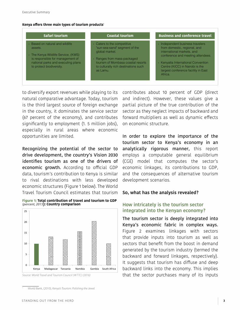
Recognizing the potential of the sector to drive development, the country’s Vision 2030 identifies tourism as one of the drivers of economic growth. According to official GDP data, tourism’s contribution to Kenya is similar to rival destinations with less developed economic structures (Figure 1 below). The World Travel Tourism Council estimates that tourism
contributes about 10 percent of GDP (direct and indirect). However, these values give a partial picture of the true contribution of the sector as they neglect impacts of backward and forward multipliers as well as dynamic effects on economic structure.
In order to explore the importance of the tourism sector to Kenya’s economy in an analytically rigorous manner, this report employs a computable general equilibrium (CGE) model that computes the sector’s economic linkages, its contributions to GDP, and the consequences of alternative tourism development scenarios.
So, what has the analysis revealed?
How intricately is the tourism sector integrated into the Kenyan economy?
The tourism sector is deeply integrated into Kenya’s economic fabric in complex ways. Figure 2 examines linkages with sectors that provide inputs into tourism as well as sectors that benefit from the boost in demand generated by the tourism industry (termed the backward and forward linkages, respectively). It suggests that tourism has diffuse and deep backward links into the economy. This implies that the sector purchases many of its inputs
Kenya offers three main types of tourism products1
Safari tourism Coastal tourism Business and conference travel
• Based on natural and wildlife assets.
• The Kenya Wildlife Service, (KWS) is responsible for management of national parks and executing plans to protect biodiversity.
• Caters to the competitive "sun-sea-sand" segment of the global market.
• Ranges from mass-packaged tourism of Mombasa coastal resorts to culturally rich destinations such as Lamu.
• Independent business travelers from domestic, regional, and international markets, and conference and meeting attendees.
• Kenyatta International Convention Centre (KICC) in Nairobi is the largest conference facility in East Africa.
Figure 1: Total contribution of travel and tourism to GDP (percent, 2015): Country comparison
Source: World Travel and Tourism Council (WTTC) (2016)
0Kenya Madagascar Tanzania Namibia Gambia South Africa
5
10
15
20
25
1 World Bank, (2010), Kenya’s Tourism: Polishing the Jewel.
Executive Summary

4 E c o n o m i c A s s e s s m e n t o f To u r i s m i n K e n y a
from domestic sources and is therefore highly integrated into the economy. More generally, compared to Tanzania2 and other countries, the backward multipliers in Kenya are strong, indicating that tourism is well integrated into the economic fabric of the country.
Non-irrigated agriculture has the highest forward linkages and hence gains the most from the generic increase in demand induced by tourism. In terms of forward linkages, there are predictable impacts on industries that are “close” to tourism such as agriculture (a key source of employment for the poor), trade, and transport, as well as surprising beneficiaries such as the education sector (Figure 2).
How important is tourism for the economy?
Since tourism in Kenya has such wide linkages across the economy, the economic impact or value of the sector will depend upon the source of change. Impacts will differ depending upon whether changes emerge due to an exogenous shock to the demand for tourism by foreigners, or exogenous shocks and changes to input costs or supplies, or due to some combination of shocks. To illustrate the importance of tourism to the economy, four hypothetical scenarios are considered to cover a range of possibilities (Table 1). The variety of scenarios explored suggest that tourism contributes between 8-14 percent to Kenya’s GDP, with highly pro-poor distributional impacts in rural areas.
Figure 2: The tourism sector’s backward and forward linkages
Source: Elaboration of Kenya SAM
00.5
11.5
22.5
33.5
44.5
5
Backward linkages Forward linkages
2 For example, in the case of exogenous investment and foreign account, the backward multiplier for tourism is 0.22 for Kenya against 0.18 for Tanzania (see Annex for details). This means that there is a greater impact in Kenya. For instance, $1 spent in Kenya induces a backward multiplier effect of 22 cents in Kenya but 18 cents in Tanzania.
Table 1: Summary of simulation scenarios to illustrate the importance of tourism to Kenya’s economy
Scenario number Scenario category Scenario category
1 Demand shock 80% decrease in foreign demand for tourism; capital is immobile
2 Demand shock 80% decrease in foreign demand for tourism; capital is immobile
3 Supply shock 80% decrease in foreign demand for tourism; capital is mobile
4 Supply shock 50% cost increase for both direct inputs and transport
Executive Summary

5S ta n d i n g O u t F r O m t h e h e r d
In the first two scenarios, there is assumed to be a decline in foreign tourist revenues. When foreign demand falls, tourism prices decline and this in turn stimulates a strong increase in domestic tourism, which partly compensates for fewer foreign tourists. The end result is a decrease in GDP of between 8 to 12 percent. The impacts fall disproportionately upon the rural poor whose incomes decline by over 10 percent. This partly reflects the links with non-irrigated agriculture, which is the primary employer of the rural poor. The next two scenarios consider supply-side shocks through cost increases. These suggest that GDP would decline by between 12 and 13 percent — a result that is robust to wide variations in the magnitude of the shocks. Again, the rural poor suffer the most with a striking 14 percent decline in their incomes. In sum, the analysis of these scenarios suggests that tourism is well integrated into the economy and makes a significant contribution, with benefits that accrue strongly to the rural poor.
While the results are to be interpreted with care because the simulated equilibria are rather distant from the baseline, they suggest that tourism is a key sector of the Kenyan economy and that its direct and indirect effects tend to be considerably larger than those credited by the national accounts.
Which product line provides the greatest boost to GDP?
The dynamic version of the CGE model investigates the consequences of equivalent growth in the safari, beach, business, and “other” categories of tourism resulting from an increase in foreign demand: foreign tourist demand (expenditure) is assumed to grow by 5 percent per year in each of the four categories.
The results show that all forms of tourism have broad economy-wide effects, though the sectoral impacts differ. The safari segment not only generates greater economic growth than each of the other forms of tourism, but would do more to address poverty problems and create rural economic opportunities. Safari tourism, alone or in combination with other forms of tourism, generates the highest GDP, with a plethora of indirect effects, especially on agriculture as the last ring of a well-developed domestic value chain. It also generates significantly greater household income as shown in Figure 3, and is also considerably more pro-poor than any of the other forms of tourism as a consequence of its closer linkages with the rural economy. In sum, when tracking the flow of expenditures through the economy, safari tourism is found to generate a greater level and spread of benefits across the economy. This is in part a consequence of the kinds of inputs purchased by this sector which have greater pro-poor benefits (for instance food purchases) and involve fewer imports than some of the other tourism sectors.
Figure 3: Impacts of the different categories of tourism on gross yearly income (KSH, millions)3
Source: Elaboration of Kenya SAM
0
20,000
40,000
60,000
80,000
100,000
120,000
140,000
160,000
Business
Rura
l poo
r
Rura
lno
n-po
or
Urb
an p
oor
Urb
anno
n-po
or
Ente
rpri
se
Gov
ernm
ent
Savi
ngs
and
inve
stm
ent
Wat
erre
sour
ces
Nat
ural
Capi
tal
Beach Safari Other
3 Enterprise refers to firm enterprises as classified in the SAM.
Executive Summary
6 E c o n o m i c A s s e s s m e n t o f To u r i s m i n K e n y a
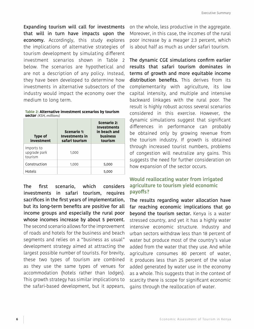
Expanding tourism will call for investments that will in turn have impacts upon the economy. Accordingly, this study explores the implications of alternative strategies of tourism development by simulating different investment scenarios shown in Table 2 below. The scenarios are hypothetical and are not a description of any policy. Instead, they have been developed to determine how investments in alternative subsectors of the industry would impact the economy over the medium to long term.
The first scenario, which considers investments in safari tourism, requires sacrifices in the first years of implementation, but its long-term benefits are positive for all income groups and especially the rural poor whose incomes increase by about 5 percent. The second scenario allows for the improvement of roads and hotels for the business and beach segments and relies on a “business as usual” development strategy aimed at attracting the largest possible number of tourists. For brevity, these two types of tourism are combined as they use the same types of venues for accommodation (hotels rather than lodges). This growth strategy has similar implications to the safari-based development, but it appears,
on the whole, less productive in the aggregate. Moreover, in this case, the incomes of the rural poor increase by a meager 2.3 percent, which is about half as much as under safari tourism.
The dynamic CGE simulations confirm earlier results that safari tourism dominates in terms of growth and more equitable income distribution benefits. This derives from its complementarity with agriculture, its low capital intensity, and multiple and intensive backward linkages with the rural poor. The result is highly robust across several scenarios considered in this exercise. However, the dynamic simulations suggest that significant differences in performance can probably be obtained only by growing revenue from the tourism industry. If growth is obtained through increased tourist numbers, problems of congestion will neutralize any gains. This suggests the need for further consideration on how expansion of the sector occurs.
Would reallocating water from irrigated agriculture to tourism yield economic payoffs?
The results regarding water allocation have far reaching economic implications that go beyond the tourism sector. Kenya is a water stressed country, and yet it has a highly water intensive economic structure. Industry and urban sectors withdraw less than 18 percent of water but produce most of the country’s value added from the water that they use. And while agriculture consumes 80 percent of water, it produces less than 25 percent of the value added generated by water use in the economy as a whole. This suggests that in the context of scarcity there is scope for significant economic gains through the reallocation of water.
Table 2: Alternative investment scenarios by tourism sector (KSH, millions)
Type of investment
Scenario 1: Investments in safari tourism
Scenario 2: Investments in beach and
business tourism
Imports to upgrade park tourism
1,000
Construction 1,000 5,000
Hotels 5,000
Executive Summary

7S ta n d i n g O u t F r O m t h e h e r dPhoto: Sarah Farhat

8 E c o n o m i c A s s e s s m e n t o f To u r i s m i n K e n y a
Allowing for a reallocation of water from irrigated agriculture to the tourism sector — or at least ensuring that supplies to the tourism sector are not diminished further — would yield high economic payoffs. The CGE model is used to explore the consequences of reallocating a small fraction (20 percent) of water from irrigated agriculture to tourism. The simulation results show that the effects on the economy are impressive. The productivity of water in tourism is high (roughly 50 KSH of product for each KSH worth of water) compared to that of agriculture (about 7.6 KSH). Since tourism generates more GDP, jobs, and rural incomes per drop of water withdrawn, this reallocation generates economic growth, higher rural incomes, and jobs. Moreover, given that the CGE analysis has shown that safari tourism generates the greatest economic growth, coupled with the fact that water is important for sustaining wildlife and ecosystems, the reallocation of water for tourism purposes would be beneficial for water-stressed Kenya. It is important to note that although the results are indicative rather than precise, they serve as a warning sign and highlight the need for a much more careful analysis of the future problems the country will face in allocating water more effectively. This is an issue that warrants greater policy discourse and deeper analysis. A number of such trade-offs are already being encountered, such as around Naivasha and Mombasa, and more will emerge in the near future as water demands increase as a result of population and economic growth, while supplies diminish, especially in key water sheds, as a consequence of climate change and habitat erosion.
Do policies aimed at conservation and sustainable development also make economic sense?
Tourism has emerged as a significant contributor to the Kenyan economy. The intensive modeling undertaken in this report suggests that the sector is deeply integrated into the economy and much of the direct and indirect activity that is induced by tourism generates significant benefits for the poor, especially in rural areas where poverty incidence is high. The safari tourism sector stands out in terms of its growth dynamism and ability to create rural economic opportunities. Thus, further expansion of this sub-sector seems warranted but it would need to be managed with considerable care.
Though tourism is an important economic driver today it faces numerous challenges in Kenya. There are deep risks that the current focus on tourist numbers rather than tourist revenue will undermine the industry and diminish the sector’s potential. Problems of congestion, overcrowding, and ecosystem degradation will inevitably worsen as more tourists crowd into diminishing and degraded habitats. Demand will eventually and inevitably decline for a visitor experience that is inferior to that offered at rival destinations. Much of Kenyan tourism is targeted at the spectrum of the market where profit margins are low and where volumes need to be high to break even. Somewhat ambitiously, Kenya’s Vision 2030 sets a target of five million tourists — which would require a four or five-fold increase in tourist numbers. Increased numbers of this magnitude would necessitate a substantial reduction in prices to attract visitors from competing market segments. Higher tourist numbers could result in lower
Executive Summary

9S ta n d i n g O u t F r O m t h e h e r d
tourist revenue if prices need to be reduced substantially to attract more visitors. It is more appropriate to target an increase in revenues from tourism rather than an increase in the number of tourists. Additionally, the popular safari destinations remain highly congested with signs of ecosystem distress and a deteriorating experience offered to tourists. This has perpetuated the dependence on low value-added segments of the market.4 Kenya operates within a globally competitive tourism industry, and it faces choices of which market segments to develop and how it can strategically compete for the global tourist dollar. In stark terms, there is a choice between the high-value low-density (HVLD) tourist market and the low-value high volume (LVHV) market. The former calls for restricting supply and targeting the high-end segment of the market, while the latter operates on slender margins, is intensely price competitive, and therefore needs to maximize volumes to make profits or break even. The latter, if unmanaged, can create a downward spiral of crowding and site degradation. Tanzania has been more successful in targeting the HVLD market, and it caters to a segment of the market where demand is relatively price inelastic; hence, it
can raise more revenue per tourist than Kenya. However, the HVLD approach is not suitable for every tourist destination and this will consequently call for a diversified approach to tourism development in Kenya, which requires a differentiated strategy that plays to the economic strengths of each attraction and asset.
Kenya’s alluring assets have created a robust tourism industry that appears to play a pivotal role in sustaining the livelihoods of the rural poor. To build upon this foundation, Kenya needs to play to the comparative advantage of each region and attraction. Going forward, the Government of Kenya (GoK) and tourism stakeholders may consider building and differentiating tourism by location (carrying capacity and accessibility), product (wildlife, beach, culture, conference, and adventure), and market segment (domestic, international, and conference). Given the variety of assets and the diversity of customers, products can be designed in multiple, interesting, and lucrative ways. The HVLD approach is not suitable for every tourist destination and this will consequently call for a diversified approach to tourism development in Kenya, and to optimize tourism as a source of economic dynamism.
4 A common sight at popular safari destinations is that of tourist vehicles queueing to view wildlife. The experience has often been compared to that of a zoo, lacking in both authenticity and quality, and as a result, few experienced wildlife enthusiasts visit Kenya’s most popular sites in peak season.
Executive Summary

10 E c o n o m i c A s s e s s m e n t o f To u r i s m i n K e n y a
Much of Kenyan tourism is targeted at the spectrum of the market where profit margins are low and where volumes need to be high to break even. Of great concern is the irreversible damage that could occur to natural habitats. Many of Kenya’s key tourist attractions are already under pressure and showing signs of degradation.
1
Photo: Sarah Farhat

11S ta n d i n g O u t F r O m t h e h e r d
Kenya’s Tourism sector: Changing Landscapesand FortunesContext
The tourism sector, especially nature-based tourism, has played a pivotal role
in shaping Kenya’s development fortunes. Tourism dominates the service sector (67 percent of the economy) and it is the third largest source of foreign exchange in the country; the World Travel Tourism Council estimates that it contributes about 10 percent of GDP, direct and indirect (as shown in Figure 3 above).5 Tourism is also a key part of the country’s economic strategy and is identified in Vision 2030 as one of the drivers of economic growth. However, the contribution of tourism to the economy — much of it derived from visits to national parks6 — is open to debate with some claiming that the sector’s contribution is actually much lower.
Kenya’s impressive tourism development is the product of early investments in protected areas and a tourism infrastructure that has drawn tourists to the country. At independence in 1963, Kenya derived the bulk of its foreign exchange from exports of tea and coffee. With declining commodity prices, the country turned to nature-based tourism, which offered an opportunity to diversify export revenues while playing to its natural comparative advantage. Today, the typical international tourist arrives on a package tour that may include a safari, a visit to the beach, or both.
Kenya offers three main types of tourism products: safari tours that vary in quality of service and price, coastal tourism that
typically caters to the highly competitive “sun — sea — sand” segment of the global market, and business and conference travel. Cultural heritage tourism activities are limited and offer potential for further development. Safari tourism is dependent on natural and wildlife assets, which are seasonal with peaks and valleys tied to animal migration patterns. Capacity is limited by the fragility of ecosystems, though there is little evidence that such constraints have influenced policies. Kenya’s coastal tourism offers products ranging from the mass-packaged tourism of Mombasa’s large coastal resorts to niche destinations. Business and conference travel is a segment with much potential. The Kenyatta International Conference Centre (KICC) in Nairobi has the largest conference chamber in East Africa and recently hosted nearly 40 heads of state and over 10,000 delegates during the Sixth Tokyo International Conference on African Development (TICAD). The Government has also recently announced plans to build a convention centre in the city of Mombasa. Moreover, Kenya is an international airline hub with direct access that far exceeds the capacity of any other country in East Africa.
There is recognition that some of the current products (e.g., nature-based tourism) are reaching their limits and there is a need to offer a more diverse set of experiences (such as conference tourism). There are encouraging trends in the industry. Local and international conference tourism has grown significantly,
5 Measuring the contribution of tourism to GDP is not a simple exercise since tourism involves a plurality of value chains that include travel, lodging, leisure activities, and many interlocking sectors and subsectors. For example, in the case of Italy, one of the world’s most sought out tourist destinations, the World Atlas estimates that tourism accounts for 19 percent of GDP, while the government declares “…the sector of tourism, including the activity it generates, contributes approximately one-third to the overall GDP by creating over one million jobs.” (http://www.esteri.it/mae/en/ministero/servizi/benvenuti_in_italia/conoscere_italia/economia.html).
6 World Travel and Tourism Council, (2012), Travel and Tourism Economic Impact 2012. Also see Figure 2.

12 E c o n o m i c A s s e s s m e n t o f To u r i s m i n K e n y a
and the Tourism Cabinet Secretary projects conference tourists will hit 130,000 by the end of 2016, up from 77,000 in 2015 and 44,000 in 2014.7 In November 2016, the government allocated Sh10 million to set-up a task force with the aim of developing a marketing strategy for conference tourism in Kenya.8 In addition, there has been a gradual increase in domestic tourism, helped by rising per capita incomes, which were responsible for the growth of the middle-class population, and there is considerable scope for expanding this market segment as shown in Figure 4.
Despite a diversifying economy and mounting challenges, tourism remains an important contributor to the Kenyan economy. Figure 4 illustrates that according to official GDP data, tourism’s contribution to Kenya is not dissimilar to rival destinations with less developed economic structures. These values give a partial picture of the true contribution of the sector as they neglect impacts of backward and forward multipliers as well as dynamic effects on economic structure. For instance, the bulk of tourists are international travelers, so variations in tourist numbers would impact external balances and the exchange rate with consequent effects in tradable goods sectors as well as the structure of the economy. It is well known that reliance on a single sector for exports (for example mining) can lead to an overvalued exchange rate that in turn impedes the development and competitiveness of other export industries9 unless the dominant exporter has deep and wide links in the rest of the economy. Capturing these trends calls for a dynamic CGE model that links each sector of the economy and allows for changes in economic
structure. These matters are addressed in greater detail in Chapters 2 and 3 of this report.
Challenges and opportunities
The short-term prospects for Kenyan tourism have been clouded by a perfect storm of misfortunes — domestic elections, insecurity, and unsustainable tourism development. Initially, security concerns surrounding the 2013 elections dampened visitor numbers. This was soon followed by the global economic slowdown
7 African Travel & Tourism Association, 23 August 2016. http://www.atta.travel/news/7129/conference-tourists-to-double-in-2016-in-kenya8 Business Daily, “Task force gets Sh10m to review Kenya’s tourism strategy,” November 9, 2016. http://www.businessdailyafrica.com/Taskforce-gets-Sh10-million-to-review-Kenya-
s-tourism-strategy/539546-3446864-6rtuhk/9 Termed the Dutch Disease.
Figure 4: Total contribution of travel and tourism to GDP (Percent, 2015)
Source: WTC (2016)
GDP share
Kenya Madagascar Tanzania Namibia Gambia South Africa0
5
10
15
20
25
Table 3: Key travel and tourism performance indicators for Kenya (2015)
Key Indicators 2015 (%)
Leisure travel spending as % of total travel spending 67.5
Business travel spending as % of total travel spending 32.5
Total tourism contribution to GDP (%) 9.9
Tourism contribution to exports (%) 14.9
Direct and Indirect (induced) employment (% total) 9.3
Direct and Indirect (induced) employment (% total) 6.2
Source: WTTC (2016)
Kenya Tourism Sector
13S ta n d i n g O u t F r O m t h e h e r d
in the Eurozone. In 2013, the damaging fire at Jomo Kenyatta International Airport and the much publicized attacks on the Westgate Mall in Nairobi added to these problems. The April 2015 massacre of college students in Garissa further fed perceptions of insecurity in the country. Despite these events, the Ministry of Tourism’s tourism diversification strategy has paid some dividends. The strategy is aimed at increasing tourism beyond coastal and wildlife safari destinations, increasing the diversity of tourism products, and increasing tourist arrivals from outside the US, UK, and Western Europe. Regarding the latter, there has since been a steady flow of tourists from Asia, albeit involving a more price–elastic (cost sensitive) segment of the market. In addition, in 2014, the government launched a Tourism Recovery Taskforce, headed by a private sector hotelier, charged with developing a comprehensive strategy for reviving tourism, including initiatives to improve security, develop infrastructure, and shift the perception of the country in foreign markets.10
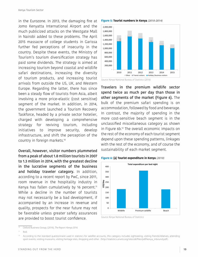
Overall, however, visitor numbers plummeted from a peak of about 1.8 million tourists in 2007 to 1.3 million in 2014, with the greatest decline in the lucrative segments of the business and holiday traveler category. In addition, according to a recent report by PwC, since 2011, room revenue in the hospitality industry in Kenya has fallen cumulatively by 16 percent.11 While a decline in the number of tourists may not necessarily be a bad development, if accompanied by an increase in revenue and quality, prospects for the near future may not be favorable unless greater safety assurances are provided to boost tourist confidence.
Travelers in the premium wildlife sector spend twice as much per day than those in other segments of the market (Figure 6). The bulk of the premium safari spending is on accommodation, followed by food and beverage. In contrast, the majority of spending in the more cost-sensitive beach segment is in the unclassified miscellaneous category as shown in Figure 6b.12 The overall economic impacts on the rest of the economy of each tourist segment depend upon these spending patterns, linkages with the rest of the economy, and of course the sustainability of each market segment.
Figure 5: Tourist numbers in Kenya (2010-2014)
Source: Kenya National Bureau of Statistics (2016)
-
200,000
400,000
600,000
800,000
1,000,000
1,200,000
1,400,000
1,600,000
1,800,000
2,000,000
2010 2011 2012 2013 2014 2015Other Transit visitors Holiday /business visitors
10 Oxford Business Group, (2016), The Report: Kenya 2016.11 Ibid.12 According to the standard questionnaire used in statistics for satellite accounts, this category includes sightseeing, visiting friends/relatives, attending
sport events, visiting museums, visiting heritage sites, shopping and other. (http://statistics.unwto.org/sites/all/files/pdf/kenya_inbound.pdf ).
Figure 6: (a) Tourist expenditure in Kenya (2010)
Source: Kenya National Bureau of Statistics
0Wildlife Premium wildlife Beach
50
100
150
200
250
300
350
400Total expenditure per bed night
US$
/day
Kenya Tourism Sector

14 E c o n o m i c A s s e s s m e n t o f To u r i s m i n K e n y a
The Kenyan tourism industry is at a crossroads and must make a strategic decision on how to develop its offerings. The industry has experienced negative medium-term trends with a decline in per capita spending, average length of stay, and hotel occupancy rates, although the last two variables show a reversal in the past few years.13 In part, this reflects the type of product that is now on offer and the emergence of competitors. The popular safari destinations remain highly congested and are increasingly targeted towards the low-margin tourist market. Despite the country’s policy of advocating spatial dispersion of tourism, marketing has continued to focus on the traditional attractions, thereby perpetuating concentration and the deterioration in the quality of the tourism products.14
Much of Kenyan tourism is targeted at the spectrum of the market where profit margins are low and where volumes need to be high to break even. While this may be a suitable
approach for some forms of tourism, it has consequences that need to be considered. Figure 7 below provides an instructive comparison between tourist numbers and revenues in Kenya and its nearest neighbor, Tanzania. Kenya and Tanzania offer similar tourism experiences — a safari that may be combined with a beach visit. According to a value chain analysis conducted by the World Travel and Tourism Council, Tanzania’s higher earnings per visitor are mostly attributable to lower congestion and its ability to attract travellers who are prepared to pay a higher price for a more authentic and exclusive wilderness experience. In other words, Tanzania caters to a segment of the market where demand is relatively price inelastic and hence it can raise more revenue per tourist than Kenya.15 There are signs though that this is changing as Tanzania also seeks to target tourist numbers; this would entail stronger competition with Kenya in the medium to short-term as both countries compete for the same niche with similar products.
Figure 6: (b) Expenditure per category
Source: Kenya National Bureau of Statistics (2016)
0102030405060
US$
708090
Beach
Acc
omm
odati
on
Food
and
beve
rage
s
Excu
rsio
n an
dpa
rk fe
es
Inla
nd t
rans
port
Out
of p
ocke
t e
xpen
ditu
re
Mis
cella
neou
s
Premium Wildlife Wildlife
13 According to the World Bank and the Kenya Economic Survey, in the years 2012-2014, tourist arrivals declined from 1.8 million to 1.3 million, while expenditure increased from $197 million to $206 million, with expenditure per-capita increasing from $108 to $153. Other accounts, such as a recent interview with the Minister of Tourism, suggest that earnings from foreign tourism had fallen to $870 million from a peak of $1.2 billion in 2011. (http://www.businessdailyafrica.com/Balala-sees-Kenya-tourism-recovering-in-2018/-/539546/3038300/-/xda2uf/-/index.html).
14 A common sight in the Masai Mara is that of tourists crowding around (say) a pride of lions, trying to get a good view. The experience has often been compared to that in a zoo, lacking in both authenticity and quality, and as a result few experienced wildlife enthusiasts visit Kenya’s most popular sites.
15 During the 2008–09 recession, tourist numbers plummeted across the globe, yet tourist numbers in Tanzania were largely unaffected (World Bank, 2016).
Figure 7: Tourism numbers and receipts – Kenya vs. Tanzania (2016)
Source: World Travel and Tourism Council (WTC) (2016)
0.0
0.2
0.4
0.6
0.8
1.0
1.2
1.4
0.0Kenya Tanzania
0.5
1.0
1.5
2.0
2.5
Visi
tor e
xpor
ts (B
, US$
)
Inte
rnati
onal
tour
ist a
rriv
als (
M)
Visitor exports (Billions, US$) International tourist arrivals (Millions)
Kenya Tourism Sector
15S ta n d i n g O u t F r O m t h e h e r d
Somewhat ambitiously, Kenya’s Vision 2030 sets a target of five million tourists — which would require a four or five-fold increase in tourist numbers. Increased numbers of this magnitude call for careful consideration of the economic and ecological consequences. A dramatic increase in tourist numbers would necessitate a substantial reduction in prices to attract visitors from competing market segments. Indeed, higher tourist numbers could well result in lower tourist revenue if prices need to be reduced (by a proportionately greater amount) to attract more visitors. Since the aim is to increase revenues, GDP, and local incomes, it is more appropriate to target an increase in revenues from tourism rather than an increase in the number of tourists.
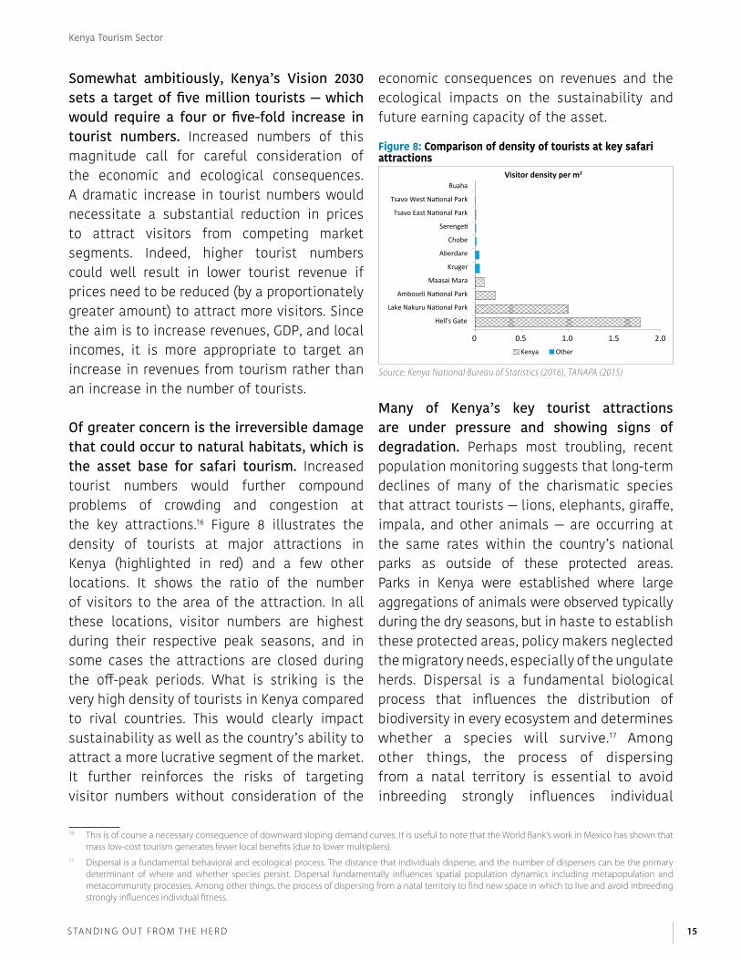
Of greater concern is the irreversible damage that could occur to natural habitats, which is the asset base for safari tourism. Increased tourist numbers would further compound problems of crowding and congestion at the key attractions.16 Figure 8 illustrates the density of tourists at major attractions in Kenya (highlighted in red) and a few other locations. It shows the ratio of the number of visitors to the area of the attraction. In all these locations, visitor numbers are highest during their respective peak seasons, and in some cases the attractions are closed during the off-peak periods. What is striking is the very high density of tourists in Kenya compared to rival countries. This would clearly impact sustainability as well as the country’s ability to attract a more lucrative segment of the market. It further reinforces the risks of targeting visitor numbers without consideration of the
economic consequences on revenues and the ecological impacts on the sustainability and future earning capacity of the asset.
Many of Kenya’s key tourist attractions are under pressure and showing signs of degradation. Perhaps most troubling, recent population monitoring suggests that long-term declines of many of the charismatic species that attract tourists — lions, elephants, giraffe, impala, and other animals — are occurring at the same rates within the country’s national parks as outside of these protected areas. Parks in Kenya were established where large aggregations of animals were observed typically during the dry seasons, but in haste to establish these protected areas, policy makers neglected the migratory needs, especially of the ungulate herds. Dispersal is a fundamental biological process that influences the distribution of biodiversity in every ecosystem and determines whether a species will survive.17 Among other things, the process of dispersing from a natal territory is essential to avoid inbreeding strongly influences individual
16 This is of course a necessary consequence of downward sloping demand curves. It is useful to note that the World Bank’s work in Mexico has shown that mass low-cost tourism generates fewer local benefits (due to lower multipliers).
17 Dispersal is a fundamental behavioral and ecological process. The distance that individuals disperse, and the number of dispersers can be the primary determinant of where and whether species persist. Dispersal fundamentally influences spatial population dynamics including metapopulation and metacommunity processes. Among other things, the process of dispersing from a natal territory to find new space in which to live and avoid inbreeding strongly influences individual fitness.
Figure 8: Comparison of density of tourists at key safari attractions
Source: Kenya National Bureau of Statistics (2016), TANAPA (2015)
0 0.5 1.0 1.5 2.0
Hell's Gate
Lake Nakuru Na nal Park
Amboseli Na nal Park
Maasai Mara
Kruger
Aberdare
Chobe
Serenge
Tsavo East Na nal Park
Tsavo West Na nal Park
RuahaVisitor density per m2
Kenya Other
Kenya Tourism Sector
16 E c o n o m i c A s s e s s m e n t o f To u r i s m i n K e n y a
fitness. As a result, wildlife depends as much on adjacent land as it does on the protected areas for continued viability. Pressures around Kenyan parks are affecting the wildlife in the parks. The way land outside of protected areas is utilized and managed will become a crucial determinant of the industry’s future. Expanding tourism to these areas remains among the most successful approaches that have been piloted — under the rubric of “ecological easements”. But the feasibility of this approach depends upon economic incentives and the opportunity costs of land.
Kenya operates within a globally competitive tourism industry, and faces choices of which market segments to develop and how to strategically compete for the global tourist dollar. In stark terms, there is a choice between the high-value low-density (HVLD) tourist market and the low-value high volume (LVHV) market. The former calls for restricting supply and targeting the high-end segment of the market, while the latter operates on thin margins, is intensely price competitive, and therefore needs to maximize volumes to make profits or break even.
The HVLD approach has several advantages for wildlife related tourism. High-value visitors are typically unaffected by turbulence in the global economy. During the 2008-2009 recession, tourist numbers plummeted across the globe, yet the high-value added tourist numbers in Tanzania were largely unaffected.18 In addition, low visitor numbers can minimize congestion at popular sites and preserve the economic value of the product by providing visitors with an authentic wilderness experience. This can
also avoid overcrowding, which has adverse ecological consequences that diminish the value of the product.
The HVLD approach is not suitable for every tourist destination and this will consequently call for a diversified approach to tourism development in Kenya. For HVLD tourism to succeed, a host of conditions must prevail: First, the product on offer must be rare or even unique. As a corollary, since such HVLD tourism assets are rare, by implication there is less competition, allowing for higher prices to be charged for the experience. HVLD tourism attracts people who care more about experience (for example, wilderness) and less about price (that is, more inelastic demand). This group might include the so-called high-net-worth individuals and also includes interest groups (hobbyists, birdwatchers, and climbers). Hence, not every destination in Kenya will fit into this category and there is a need for a differentiated strategy that plays to the economic strengths of each attraction and asset. Clearly, uncongested and more pristine parts of the wildlife sector can be developed for HVLD tourism in ways that deepen economic linkages, protect the ecosystem, and generate revenues. Much of beach tourism on the other hand remains highly competitive, though there are higher valued niche segments of the market. The sun-sea-sand product is widely available in almost every tropical coastal country, so competition is intense and consumer choices are determined by costs. A careful segmentation of the market based upon the economic potential and capacity of each asset will be needed to strike the right balance between volume, value, and sustainability.
18 World Bank, 2016.
Kenya Tourism Sector
17S ta n d i n g O u t F r O m t h e h e r d
Concluding comments
Tourism can be source of economic dynamism. This is evident from the experience of countries as diverse as Costa Rica, Switzerland, Bhutan, Australia, and New Zealand. Indeed, each of these countries has built upon its natural comparative advantage by playing to its strengths in ways that have maximized and sustained the value of its assets. Among these success stories, there has been recognition that revenues are generated from natural assets that can be degraded and depleted. Investors and decision makers with short horizons will have little incentive to consider the longer-term
consequences of asset depletion. Thus, there is a need for appropriate and sagacious policies, laws, and systems that assure stewardship and longer term sustainability of the asset. In addition, examples abound where tourism and the related investment incentives, when managed poorly, create “enclave industries” with few linkages to the rest of the economy. To maximize economic payoffs, incentives and economic policies are needed that promote linkages with the rest of the economy to boost employment, GDP, and incomes from the sector. This has been done in countries with success stories.
Kenya Tourism Sector

Tourism is a key sector of Kenya’s economy, with wide backward and forward linkages and pro-poor distributional impacts. After the transport and entertainment related sectors, a primary beneficiary of the sector is non-irrigated agriculture, which is a key source of employment for the poor.
2
Photo: Sarah Farhat
19S ta n d i n g O u t F r O m t h e h e r d
The Big Question: How vital is Tourism for the Kenyan economy? Context
This chapter investigates the importance of tourism to the Kenyan economy. It
recognizes that tourism is a major sector of the economy and that variations in the sector will have impacts that reverberate throughout the economy, with magnitudes that are defined
by the extent of linkages between sectors and the multiplier effects of each. To capture these trends, a standard Computable General Equilibrium (CGE) model of the Kenyan economy has been built. Box 1 provides a brief description of the model and the Annex discusses more technical details.
Box 1: Description of the CGE Model
The CGE was formulated using fixed input-output coefficients for intermediate inputs, linear expenditure systems for household consumption, and Cobb-Douglas specifications for demand for factors of production. Trade is modeled assuming that internationally tradable and non-tradable goods are imperfect substitutes.
The main structure of the model is based on the reasonable assumption that intermediate inputs are not substitutes for each other in production technology. The main features involve profit maximization by producers, utility maximization by households, mobility of labor, and competitive markets. It is a static and single-country CGE model extended to incorporate both national and international tourism and its relations with the other sectors and environmental variables.
Tourism is modeled as an industry providing a specific product and by distinguishing the different components of the domestic value chain. Foreign tourist demand is divided into four components: business, beach, safari, and ‘other’, the latter category being a miscellaneous category that includes the relatively new forms of ecological and domestic tourism.
The model has been calibrated using the SAM estimated for 2014 so that the model parameters are such that the CGE solution reproduces the 2014 data as a baseline reference. Two alternative closure rules have been used for the first experiments: (1) exogenous government expenditure with flexible exchange rate, and (2) fixed exchange rate with exogenous foreign trade. In both cases, closure rules are “Keynesian”, in the sense that they are compatible with less than full employment. Because the model is based on an extended Environmental SAM, it generates statistics of both GDP and green GDP (defined as GDP plus the additional value added imputable to the environmental components).
An important caveat must be noted when interpreting the results. Projecting future economic performance is a complex and hazardous endeavor. Future changes in economic structures, technological innovations, policies, political priorities, and consumer preferences cannot be known. As with all modeling exercises, the analysis is based on a litany of assumptions, driven by data availability and computational constraints. The exercise provides projections based upon hypothetical scenarios, not forecasts of the economy.
20 E c o n o m i c A s s e s s m e n t o f To u r i s m i n K e n y a
At the outset, it must be emphasized that as with any technique, the CGE approach carries both advantages and weaknesses. An advantage of CGE models is that they are well suited to capture inter-linkages between sectors of the economy. A second benefit is that CGE models can also be used for scenario analyses, especially in data sparse environments where statistical evidence is lacking. The major disadvantage of the approach is that the models and results remain highly sensitive to assumptions about functional forms and estimates of parameters concerning, for example, demand and supply functions, elasticities of substitution, and degree of non-linearity of model formulation. Furthermore, complexity of the models imply that interpretation of results are rendered difficult. Notwithstanding these caveats, the approach is arguably amongst the most robust and comprehensive ways of understanding sector linkages and determining their importance. The CGE built for this exercise draws upon a number of such models that have been developed for Kenya. Backward and forward linkages of the tourism sector
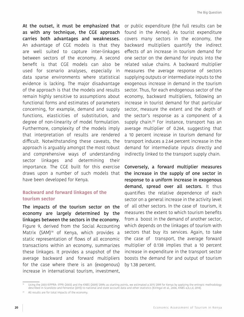
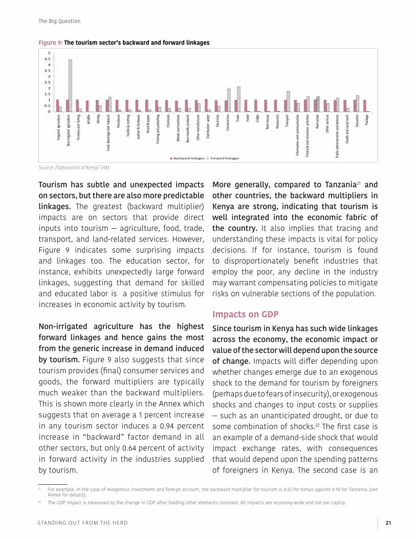
The impacts of the tourism sector on the economy are largely determined by the linkages between the sectors in the economy. Figure 9, derived from the Social Accounting Matrix (SAM)19 of Kenya, which provides a static representation of flows of all economic transactions within an economy, summarizes these linkages. It provides a snapshot of the average backward and forward multipliers for the case where there is an (exogenous) increase in international tourism, investment,
or public expenditure (the full results can be found in the Annex). As tourist expenditure covers many sectors in the economy, the backward multipliers quantify the indirect effects of an increase in tourism demand for one sector on the demand for inputs into the related value chains. A backward multiplier measures the average response of sectors supplying outputs or intermediate inputs to the exogenous increase in demand in the tourism sector. Thus, for each endogenous sector of the economy, backward multipliers, following an increase in tourist demand for that particular sector, measure the extent and the depth of the sector’s response as a component of a supply chain.20 For instance, transport has an average multiplier of 0.264, suggesting that a 10 percent increase in tourism demand for transport induces a 2.64 percent increase in the demand for intermediate inputs directly and indirectly linked to the transport supply chain.
Conversely, a forward multiplier measures the increase in the supply of one sector in response to a uniform increase in exogenous demand, spread over all sectors. It thus quantifies the relative dependence of each sector on a general increase in the activity level of all other sectors. In the case of tourism, it measures the extent to which tourism benefits from a boost in the demand of another sector, which depends on the linkages of tourism with sectors that buy its services. Again, to take the case of transport, the average forward multiplier of 0.138 implies that a 10 percent increase in expenditure in the transport sector boosts the demand for and output of tourism by 1.38 percent.
19 Using the 2003 KIPPRA- IFPRI (2003) and the KNBS (2009) SAMs as starting points, we estimated a 2015 SAM for Kenya by applying the entropic methodology described in Scandizzo and Ferrarese (2015) to national and state account data and other statistics (Kiringai et al., 2006, KNBS a,b,c,d, 2014).
20 All results are for total impacts of the economy.
The Big Question
21S ta n d i n g O u t F r O m t h e h e r d
Tourism has subtle and unexpected impacts on sectors, but there are also more predictable linkages. The greatest (backward multiplier) impacts are on sectors that provide direct inputs into tourism — agriculture, food, trade, transport, and land-related services. However, Figure 9 indicates some surprising impacts and linkages too. The education sector, for instance, exhibits unexpectedly large forward linkages, suggesting that demand for skilled and educated labor is a positive stimulus for increases in economic activity by tourism.
Non-irrigated agriculture has the highest forward linkages and hence gains the most from the generic increase in demand induced by tourism. Figure 9 also suggests that since tourism provides (final) consumer services and goods, the forward multipliers are typically much weaker than the backward multipliers. This is shown more clearly in the Annex which suggests that on average a 1 percent increase in any tourism sector induces a 0.94 percent increase in “backward” factor demand in all other sectors, but only 0.64 percent of activity in forward activity in the industries supplied by tourism.
More generally, compared to Tanzania21 and other countries, the backward multipliers in Kenya are strong, indicating that tourism is well integrated into the economic fabric of the country. It also implies that tracing and understanding these impacts is vital for policy decisions. If for instance, tourism is found to disproportionately benefit industries that employ the poor, any decline in the industry may warrant compensating policies to mitigate risks on vulnerable sections of the population. Impacts on GDPSince tourism in Kenya has such wide linkages across the economy, the economic impact or value of the sector will depend upon the source of change. Impacts will differ depending upon whether changes emerge due to an exogenous shock to the demand for tourism by foreigners (perhaps due to fears of insecurity), or exogenous shocks and changes to input costs or supplies — such as an unanticipated drought, or due to some combination of shocks.22 The first case is an example of a demand-side shock that would impact exchange rates, with consequences that would depend upon the spending patterns of foreigners in Kenya. The second case is an
Figure 9: The tourism sector’s backward and forward linkages
Source: Elaboration of Kenya SAM
0
0.5
1
1.5
2
2.5
3
3.5
4
4.5
5
Backward linkages Forward linkages
21 For example, in the case of exogenous investment and foreign account, the backward multiplier for tourism is 0.22 for Kenya against 0.18 for Tanzania (see Annex for details).
22 The GDP impact is measured by the change in GDP after holding other elements constant. All impacts are economy-wide and not per capita.
The Big Question

22 E c o n o m i c A s s e s s m e n t o f To u r i s m i n K e n y a
example of supply-side shocks whose impacts would depend on the extent to which cheap substitutes are available for Kenyan agricultural produce. Since the effects differ, broad generalizations about the “contribution” of tourism to the economy would be misleading. The source of change in the sector needs to be specified and the consequences inferred through the many linkages of tourism in the economy. Put simply, a statement such as “what is the contribution of tourism to GDP?” has little meaning unless one specifies the source and magnitude of the decline (or increase). A snapshot of a single point in time, in fact, as is done in national accounts, would not yield a measure of the real importance of tourism because it would neglect all dynamic and indirect effects on the economy.
To illustrate the importance of tourism to the economy, four hypothetical scenarios are considered to cover a range of possibilities. In the first two scenarios, there is assumed to be an 80 percent decline in foreign demand for tourism. This is arguably a relevant scenario given security concerns within Kenya, global turbulence, and rising foreign competition. Any of these factors could lead to changes in foreign tourist demand. The eventual impacts of an external shock of any kind will depend crucially upon how exchange rates are impacted. To capture the full range of possible outcomes two extreme cases are considered. In the first case it is assumed that capital is immobile (endogenous interest rates), and in the second case capital is assumed to be mobile (exogenous interest rates). The extent of capital mobility will influence a host of
relevant economic parameters such as capital that is available for investment, the exchange rate, and the distribution and level of factor demand in the economy.
In the third scenario it is assumed that the same level of contraction in tourism revenues is caused by a supply-side shock. In this scenario, there is an overall cost increase of 100 percent for direct inputs and 50 percent for transport. Once the shock occurs, the resources devoted to tourism accrue to other sectors (and are optimally allocated by the forces of demand and supply). A 100 percent increase in price is chosen because it yields approximately the same reduction of tourism revenue as a demand shock that causes a decline of 80 percent of foreign tourism (which is the hypothesis of the demand shock scenario). The impact of a supply-side shock on the economy, however, is different from the demand shock since it affects industry costs and induces changes in foreign tourist demand given that it affects the exchange rate (increase in the ratio of domestic to international prices). This in turn spreads the impacts of the industry cost increase to all sectors of the economy.
Finally, to test the robustness of the results, in the fourth scenario, the cost increase is assumed to be much lower, at 50 percent. This turns out to be equivalent to the GDP impact of a demand shock (under the capital mobility assumption). The results reinforce the conclusion that even when the final GDP impact is the same, the distributional and sectoral impacts differ depending upon the source of the shock.
The Big Question

23S ta n d i n g O u t F r O m t h e h e r d
Demand shocks: Decline in foreign demand
The overall results suggest that a demand shock (80 percent decline in foreign tourist revenue) would result in an 8 to 12 percent decline in GDP with impacts that are disproportionately felt by the rural poor. The results are summarized in columns 1 and 2 in Table 4 below. There is a fall in GDP of between 8 to 12 percent depending on whether capital is assumed to be internationally immobile (and interest rates endogenous) or internationally mobile (with interest rates exogenous). In both cases, when foreign demand falls, tourism prices decline, and this in turn stimulates a strong increase in domestic tourism, which partly compensates for fewer foreign tourists. But since foreign and domestic tourism are not perfect substitutes (foreigners spend more and differently), there is an overall decline in demand and GDP. The decline is more dramatic with mobile capital as lower returns to capital in Kenya induce a migration of capital overseas.
Table 5 charts the resulting distributional impacts. Clearly, the rural poor suffer the most and experience a 9 to 12 percent decline in their incomes. Overall, gross incomes drop by 10 to 15 percent. The clear implication of this exercise is that foreign tourism is a pro-poor source of rural income with non-trivial contributions to GDP. There is a decline in tax revenues too of
11 to 15 percent, which in turn could constrain the government’s capacity to neutralize the adverse impacts on the poor.
Supply-side shocks
Supply-side shocks of equivalent magnitude (on tourist industry revenue) have larger, adverse GDP impacts and distributional consequences. Two supply side shocks are considered (scenario 3 and 4). In scenario 3, tourism sector costs rise by 100 percent. This generates a loss in tourist revenue of the same magnitude as with the foreign demand shock considered earlier. In scenario 4, industry costs rise by about 50 percent (this induces a reduction in value added of the same magnitude as the demand shock with internationally mobile capital). In both cases, there is a reallocation of economic activity, with resources absorbed at the higher prices by other sectors. The results are summarized in columns 3 and 4 of Table 4. The impacts on the economy are now larger in both scenarios with 12-13 percent loss in GDP.
Moreover, despite the large differences in the cost increases assumed (100 percent in the first scenario versus 50 percent in the second), the difference in impact on GDP is trivially small (less than 1 percent point). This result has two implications: First, it suggests that the outcomes are reasonably robust to changes
Scenario number Scenario category Key assumptions
1 Demand shock 80% decrease in foreign demandfor tourism; capital is immobile
2 Demand shock 80% decrease in foreign demandfor tourism; capital is immobile
3 Supply shock 80% decrease in foreign demandfor tourism; capital is immobile
4 Supply shock 80% decrease in foreign demandfor tourism; capital is immobile
The Big Question

24 E c o n o m i c A s s e s s m e n t o f To u r i s m i n K e n y a
in costs, implying that the contribution of the tourism sector to GDP is in the range of 12 to 13 percent when changes originate from the supply side. Second, the result illustrates the self-correcting (equilibrating) feature of a general equilibrium system — price changes act as a shock absorber in a general equilibrium system. If a shock induces positive / negative multiplier effects, prices in the relevant sectors tend to increase / decrease, which in turn moderates the impacts of the shock. It is worth noting that the differences would be even smaller under the assumption of endogenous interest rates (and capital internationally immobile) since capital prices would also fall in response to the shocks. Thus, while increases in industry costs
disrupt the tourism value chain and all the value chains related to the tourism industry, as well as disrupts both the domestic and foreign tourist sub-sectors, the model suggests that the Kenyan economy exhibits a high level of resilience.
Table 5 shows that rural incomes fall by about 13 to 14 percent. Again, the pro-poor impacts of tourism emerge in this scenario too. One reason for this is shown in Figure 9 (above); observe that the biggest backward linkage is with non-irrigated agriculture — which is the source of employment of the poorest in Kenya. Tax and tariff revenues decline by about 30 percent in these scenarios.
Table 4: Impacts of shocks on industry-wide tourism (Percent)23
Value added components
Demand shock with capital internationally
immobile
Demand shock with capital internationally
mobile
Demand shock with capital internationally
mobile
Demand shock with capital internationally
mobile
Skilled labor 10.96 13.57 14.03 12.67
Semi-skilled labor 7.32 10.61 13.50 12.48
Unskilled labor 9.98 12.93 10.52 9.66
Capital 8.10 12.11 14.22 13.06
Land 3.88 6.79 7.04 6.44
Blue Water24 7.78 10.12 7.38 6.76
Green Water25 13.17 14.57 7.22 6.62
Non renewable natural resources 26.52 27.77 13.16 12.16
Savanna and forest habitat 15.34 18.26 12.72 11.74
Direct taxes 9.41 9.97 11.04 10.14
Import tariffs 6.23 10.29 11.05 10.14
Sales taxes 10.77 14.14 12.22 10.83
Green GDP 8.48 11.95 13.01 11.92
GDP 8.06 11.80 13.37 12.0Source: Elaboration of Kenya SAM
23 These are demand and supply shocks, and by industry we refer to value added. 24 Blue water is surface water.25 Green water is water held in soils and available for use by plants.
The Big Question
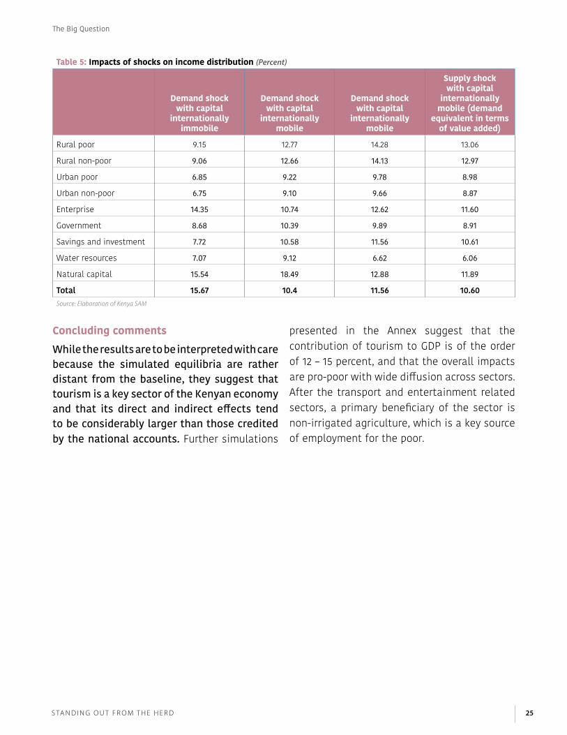
25S ta n d i n g O u t F r O m t h e h e r d
Table 5: Impacts of shocks on income distribution (Percent)
Demand shock with capital
internationally immobile
Demand shock with capital
internationally mobile
Demand shock with capital
internationally mobile
Supply shock with capital
internationally mobile (demand
equivalent in terms of value added)
Rural poor 9.15 12.77 14.28 13.06
Rural non-poor 9.06 12.66 14.13 12.97
Urban poor 6.85 9.22 9.78 8.98
Urban non-poor 6.75 9.10 9.66 8.87
Enterprise 14.35 10.74 12.62 11.60
Government 8.68 10.39 9.89 8.91
Savings and investment 7.72 10.58 11.56 10.61
Water resources 7.07 9.12 6.62 6.06
Natural capital 15.54 18.49 12.88 11.89
Total 15.67 10.4 11.56 10.60Source: Elaboration of Kenya SAM
Concluding comments
While the results are to be interpreted with care because the simulated equilibria are rather distant from the baseline, they suggest that tourism is a key sector of the Kenyan economy and that its direct and indirect effects tend to be considerably larger than those credited by the national accounts. Further simulations
presented in the Annex suggest that the contribution of tourism to GDP is of the order of 12 – 15 percent, and that the overall impacts are pro-poor with wide diffusion across sectors. After the transport and entertainment related sectors, a primary beneficiary of the sector is non-irrigated agriculture, which is a key source of employment for the poor.
The Big Question
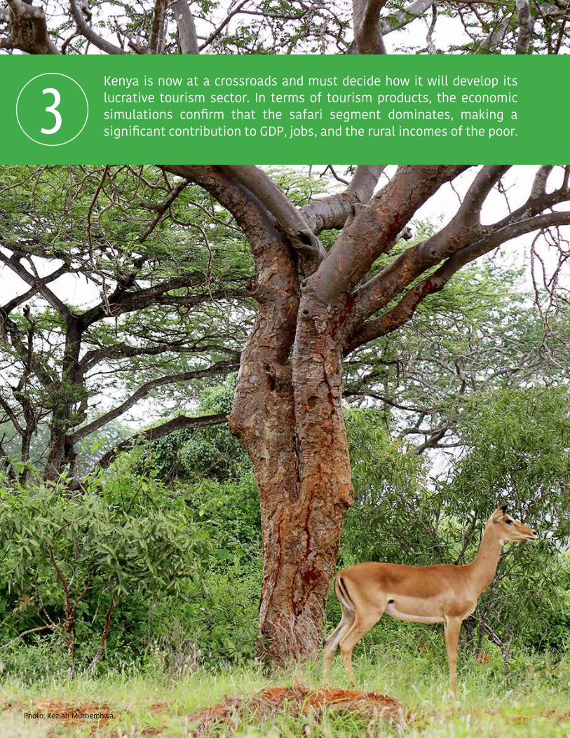
Kenya is now at a crossroads and must decide how it will develop its lucrative tourism sector. In terms of tourism products, the economic simulations confirm that the safari segment dominates, making a significant contribution to GDP, jobs, and the rural incomes of the poor.3
Photo: Keziah Muthembwa

27S ta n d i n g O u t F r O m t h e h e r d
Alternative scenarios for Kenya’s Tourism Development: A Dynamic AssessmentContext
The objective of this chapter is to explore the dynamic implications of different
growth strategies in the tourism sector on Kenya’s economic growth and the distribution of income. Typically, investments in sectors will be guided by the returns to investors and the availability of other inputs such as the supply of land or labor, that in turn determine the ability to respond to an increase in demand. As an example, if there is insufficient growth in labor supply, the responsiveness of a labor intensive industry to higher demand will be constrained. In the tourism context, these issues are especially relevant since the magnitude and nature of backward linkages vary between the different types of tourism (safari, beach, business, and other). Hence, the availability
of resources over time will determine how the economy responds to changes in any of these sub-sectors of tourism. The dynamic component is also important for policy decisions. Policies that neglect incentives to invest in a sector may end up being counterproductive if they dampen incentives and hence growth in the sector. To capture these features it is necessary to introduce a temporal dimension into the analysis, which calls for a dynamic CGE model, described briefly in Box 2 below.
To assess how well the dynamic model performs, it is instructive to compare projections with past outcomes. CGE models are not designed to capture short-term volatility, which is better analyzed through statistical modeling; instead, the CGE approach seeks to assess long-term growth trajectories.
Box 2: The dynamic CGE model
The task of introducing dynamic features in a CGE is conceptually straightforward but computationally complex. On the one hand, it amounts to replicating the static model over time periods – or equivalently adding a time subscript to the variables in the static model. On the other hand, solving intertemporal optimization problems are notoriously difficult, so the model needs to be simplified along a number of dimensions to be rendered tractable.
Recognizing these challenges, a recursive dynamic version of the static CGE model was developed with decision-making linked across periods. The model contains a capital updating module that allows capital to flow between sectors as a result of increased demand for capital goods in one period that leads to an increase in productive capacity in a future period. The lag between investment and increased production can be interpreted as the time it takes to build new capacity. The demand for investment is assumed to be a function of income and the price of capital.
Given these characteristics, the model generates a sequence of static equilibria, which reflect a path of continuous adjustment of the main economic variables. In turn, this can be seen as the result of the attempt of consumers and producers to respond to incentives by updating their decisions in light of the new evidence. To reflect this process, in each iteration, a new static equilibrium and a new SAM are computed as the basis for the computation of next period iteration.

28 E c o n o m i c A s s e s s m e n t o f To u r i s m i n K e n y a
The results for projections from 2010 - 2014 are shown in Figure 10 below, and suggest that the model tracks the trends in the Kenyan economy with reasonable accuracy, but as would be expected, fails to project short-term cyclical fluctuations.
Consequences of international tourism growth
The income and distributional consequences of further tourism development will vary depending upon the sub-sector of tourism that grows. Spending patterns amongst the different classes of tourists vary and the linkages with the rest of the economy also differ. To investigate the consequences of developing the different types of tourism, the first set of simulations consider four scenarios where foreign tourist demand (expenditure) is assumed to grow by 5 percent per year (roughly 20,000 million Kenyan Shillings) in each of the four categories of tourism: (i) business tourism, (ii) beach tourism, (iii) safari tourism, and (iv) other types of tourism.
All forms of tourism have broad economy-wide effects, though the sectoral impacts differ. Tables 6-8 present the summary results of the impact of the four different forms of tourism, considered as alternatives, on the economic activities for the terminal year of the simulation (which is fixed conventionally as the 15th year). While all forms of tourism appear to have comparable effects on the diversification of the economy and affect all sectors, there are significant differences too. Business tourism has a larger impact on growth and investment in hotels, trade, transportation, and package tours. In contrast, safari tourism appears to have a much higher impact on agriculture, both irrigated and non-irrigated, and investment in lodges. Impact on hotels is highest for the generic “other forms of tourism” category, which also appears to favor restaurant and trade.
The impacts on the economy are widespread, indicating a significant depth of the value chain of the different types of tourism. Safari tourism, alone or in combination with other forms of tourism, seems to dominate and generates the highest GDP, with a plethora of indirect effects, especially on agriculture26 as the last ring of a well-developed domestic value chain (Table 6). This type of tourism seems to be much more environmentally benign too and is less demanding in terms of water and other natural resources (savanna land and forests). Safari tourism also provides a boost to other natural resource sectors such as forestry and fishing and wildlife, as shown in Table 7. Its multiplier effect on the hotel component of the tourism industry, on the other hand, is limited, and the larger effect on this activity appears to originate from the “other” category, which
Figure 10: Comparison between data and simulations of GDP growth (2010-2014)
Source: Elaboration of the Kenya CGE model and Kenya National Bureau of Statistics
0
1
2
3
4
5
6
7
8
9
2011/2010 2012/2011 2013/2012 2014/2013
GDP
gro
wth
rate
(%)
GDP growth simulated GDP growth 2010-2014
26 The input output SAM coefficient of Safari Tourism for irrigated agriculture is about 0.014 (i.e. about 1 percent of total tourist expenditure), while for the other types of tourism it is only about 0.2 percent. This large difference is due to a higher direct consumption of fruits and vegetables, and to the fact that agriculture and safari tourism are complements (as agro-tourism) in an increasing number of Safari packages. See, for example: http://www.ecoadventuresafrica.com/safari/AgriTourism
Alternative Scenarios

29S ta n d i n g O u t F r O m t h e h e r d
Table 6: Terminal year impact of tourism on economy activity levels (KSH, millions)
Activity/SectorTypes of Tourism
Business Beach Safari Other
Irrigated agriculture 3,252 3,046 25,982 2,732
Non-irrigated agriculture 20,495 20,496 30,933 19,583
Forestry and fishing -30 -155 0.550 -129
Wildlife 141 138 2,059 130
Mining 5,902 5,098 7,918 5,073
Food, beverage and tobacco 11,049 12,090 11,879 11,116
Petroleum 1,072 1,214 1,757 843
Textile & clothing 1,174 1,007 1,523 1,018
Leather & footwear 203 164 0,374 167
Wood & paper 2,604 2,411 2,595 2,459
Printing and publishing 5,192 4,870 6,524 4,785
Chemicals 1,678 1,636 2,247 1,692
Metals and machines 1,560 1,463 2,090 1,489
Non metallic products 4,207 3,295 6,808 3,289
Other manufactures 11,922 11,288 12,277 11,395
Distribution water 3,117 2,706 11,330 2,778
Electricity 12,927 12,669 12,613 13,820
Construction 2,167 1,150 5,835 1,327
Trade 58,619 65,106 57,861 55,756
Hotel 28,608 25,403 12,820 39,552
Lodge 1,011 6,567 15,209 6,494
Rent house 13,814 20,185 3,467 19,278
Restaurant 23,164 21,092 19,012 20,860
Transport 136,180 124,230 114,067 122,516
Information and communication 10,085 9,551 9,426 9,548
Financial and insurance activities 18,675 19,798 18,013 18,888
Real estate 2,425 2,292 3,451 2,907
Other services 7,515 6,962 7,314 7,102
Public administration and defence 4,395 5,415 5,562 6,672
Health and social work 33,533 25,205 60,472 24,233
Education -505 889 -3,226 1,916
Package Tours 29,468 29,590 22,870 26,311
Total 455,620 446,871 491,611 445,600Source: Elaboration of the Kenya CGE model
Alternative Scenarios
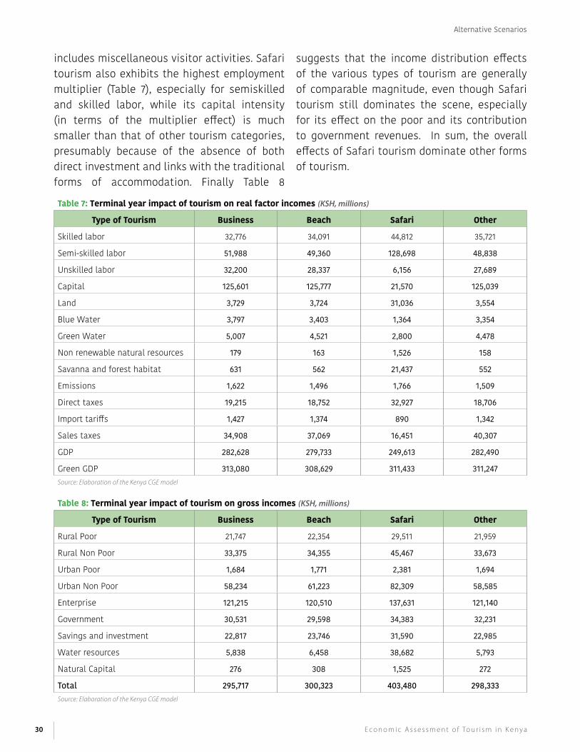
30 E c o n o m i c A s s e s s m e n t o f To u r i s m i n K e n y a
includes miscellaneous visitor activities. Safari tourism also exhibits the highest employment multiplier (Table 7), especially for semiskilled and skilled labor, while its capital intensity (in terms of the multiplier effect) is much smaller than that of other tourism categories, presumably because of the absence of both direct investment and links with the traditional forms of accommodation. Finally Table 8
suggests that the income distribution effects of the various types of tourism are generally of comparable magnitude, even though Safari tourism still dominates the scene, especially for its effect on the poor and its contribution to government revenues. In sum, the overall effects of Safari tourism dominate other forms of tourism.
Table 7: Terminal year impact of tourism on real factor incomes (KSH, millions)
Type of Tourism Business Beach Safari Other
Skilled labor 32,776 34,091 44,812 35,721
Semi-skilled labor 51,988 49,360 128,698 48,838
Unskilled labor 32,200 28,337 6,156 27,689
Capital 125,601 125,777 21,570 125,039
Land 3,729 3,724 31,036 3,554
Blue Water 3,797 3,403 1,364 3,354
Green Water 5,007 4,521 2,800 4,478
Non renewable natural resources 179 163 1,526 158
Savanna and forest habitat 631 562 21,437 552
Emissions 1,622 1,496 1,766 1,509
Direct taxes 19,215 18,752 32,927 18,706
Import tariffs 1,427 1,374 890 1,342
Sales taxes 34,908 37,069 16,451 40,307
GDP 282,628 279,733 249,613 282,490
Green GDP 313,080 308,629 311,433 311,247Source: Elaboration of the Kenya CGE model
Table 8: Terminal year impact of tourism on gross incomes (KSH, millions)
Type of Tourism Business Beach Safari Other
Rural Poor 21,747 22,354 29,511 21,959
Rural Non Poor 33,375 34,355 45,467 33,673
Urban Poor 1,684 1,771 2,381 1,694
Urban Non Poor 58,234 61,223 82,309 58,585
Enterprise 121,215 120,510 137,631 121,140
Government 30,531 29,598 34,383 32,231
Savings and investment 22,817 23,746 31,590 22,985
Water resources 5,838 6,458 38,682 5,793
Natural Capital 276 308 1,525 272
Total 295,717 300,323 403,480 298,333Source: Elaboration of the Kenya CGE model
Alternative Scenarios

31S ta n d i n g O u t F r O m t h e h e r d
The simulations suggest that safari tourism provides the more effective strategy for boosting growth throughout the economy as well as the incomes of the rural poor. As Figure 11 shows, the distributional impacts differ across the categories of tourism. Safari tourism generates significantly greater household income. It is also considerably more pro-poor than the other forms of tourism. This is perhaps a consequence of the closer linkages with the rural economy than those exhibited by other forms of tourism. In sum, if there is a choice to be made between developing the different types of tourism growth, the safari segment would not only generate greater economic growth but would do more to address poverty problems than the other forms of tourism.
Alternative strategies of tourism development
Expanding tourism will call for investments that will in turn have impacts upon the economy. Accordingly, this section further explores the implications of alternative strategies of tourism development by simulating different investment scenarios shown in Table 9. Needless to say, other scenarios involving “soft” investments could
be developed but are not considered in this exercise. The scenarios are structured as investment programs over a period of seven years and include an implementation phase of two years and an operational phase of five years. In addition to the physical investment, however, which is assumed to be just the start of the strategy, the scenarios differ because of the choice of the sector development patterns. Thus, while direct outlays for the investment are assumed to be the same, effective costs and benefits vary endogenously since further investments are generated and interact differently with the other economic variables. The backdrop is an economy that grows at an overall rate of 5 percent a year.
Scenario 1: Investments in safari tourism
The first scenario considers investments in safari tourism. Physical investment can take several forms but would in most cases include construction (roads, facilities, and services), some of which could be imported to cater to special tourist niches. This scenario is assumed to attract higher quality lower density tourists. Thus, in this scenario, it is assumed that in the first two years of implementation, a reduction of safari tourism occurs as a consequence of the temporary disruption of the safari facilities
Figure 11: Impacts of the simulation results on overall income (KSH, millions)
Source: Elaboration of the Kenya CGE model
Rura
l poo
r
Rura
l non
-poo
r
Urba
n po
or
Urba
n no
n-po
or
Ente
rpris
e
Gove
rnm
ent
Savi
ngs a
ndin
vest
men
t
Wat
er re
sour
ces
Natu
ral c
apita
l
160,000
140,000
120,000
100,000
80,000
60,000
40,000
20,000
0
Business Beach Safari Other
Table 9: Initial investments in tourism by sector (KSH, millions)
Type of investment
Scenario 1: Investments in safari tourism
Scenario 2: Investments in beach and
business tourism
Imports to upgrade park tourism 1,000
Construction 1,000 5,000
Hotel 5,000Source: Authors’ hypothesis
Alternative Scenarios

32 E c o n o m i c A s s e s s m e n t o f To u r i s m i n K e n y a
and an attempt to reorganize park tourism along new and more productive lines. These would include fewer package tours and more selective and secure ways of lodging and transportation.
This has the consequence of thinning tourism in the short-run, but boosting it in the medium-run. As Tables 10 (a) and (b) show, this scenario requires sacrifices in the first years of implementation. The Table shows that in the initial investment phase, when there is a build-up of investments, there is a slow-down of activity. In the long-term, however, benefits are positive for all income groups and especially
the rural poor, whose incomes increase by about 5 percent (Figure 12).
Figure 12: Impact of investments in safari tourism on incomes (KSH, millions)
Source: Elaboration of the Kenya CGE model
8,000
-6,000
-4,000
-2,000
0
2,000
4,000
6,000
8,000
Income effect of safari tourism strategy (yearly)
1 2 3 4 5 6 7
Rural Poor Rural Non Poor Urban Poor Urban Non Poor
KSH,
mill
ions
Year
Table 10: (a) Safari tourism development scenario (KSH, millions)
Year 1 2 3 4 5 6 7
Business tourism (international) -231 -292 366 619 916 501 273
Beach tourism (international) -139 -175 219 371 549 300 163
Safari tourism (international) -10,483 -10,611 10,764 16,302 21,940 11,071 5,586
Other tourism (international) -74 -93 117 198 293 160 87Source: Elaboration of the Kenya CGE model
(b) Impact of safari tourism strategy on incomes (KSH, millions)
Year 1 2 3 4 5 6 7
Rural poor -2,090.90 -1,021.6s3 1,033.41 1,573.90 2,132.08 1,083.55 548.85
Rural non-poor -3,225.25 -1,578.91 1,599.64 2,438.44 3,305.73 1,681.09 852.14
Urban poor -164.55 -80.87 81.72 124.63 169.23 86.28 43.76
Urban non-poor -5,687.67 -2,795.10 2,824.70 4,308.27 5,849.89 2,982.29 1,512.60
Baseline (A)Long Term Net Present
Value (NPV) (B/A)%
Rural poor (B) % (B/A) 4.8
Rural non-poor 1,378.728 66,686.7 4.8
Urban poor 91.246 3,422.9 3.8
Urban non-poor 3,200.049 118,327.9 3.7Source: Elaboration of the Kenya CGE model
Alternative Scenarios

33S ta n d i n g O u t F r O m t h e h e r dPhoto: Keziah Muthembwa
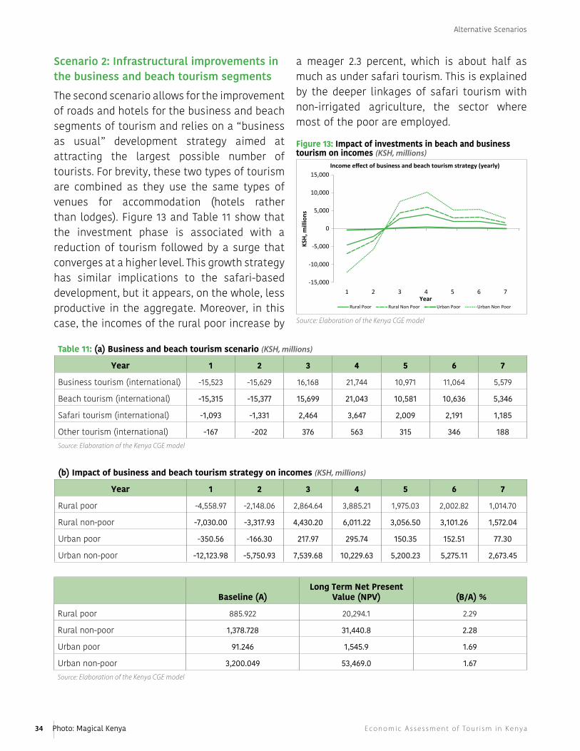
34 E c o n o m i c A s s e s s m e n t o f To u r i s m i n K e n y a Photo: Magical Kenya
Scenario 2: Infrastructural improvements in the business and beach tourism segments
The second scenario allows for the improvement of roads and hotels for the business and beach segments of tourism and relies on a “business as usual” development strategy aimed at attracting the largest possible number of tourists. For brevity, these two types of tourism are combined as they use the same types of venues for accommodation (hotels rather than lodges). Figure 13 and Table 11 show that the investment phase is associated with a reduction of tourism followed by a surge that converges at a higher level. This growth strategy has similar implications to the safari-based development, but it appears, on the whole, less productive in the aggregate. Moreover, in this case, the incomes of the rural poor increase by
a meager 2.3 percent, which is about half as much as under safari tourism. This is explained by the deeper linkages of safari tourism with non-irrigated agriculture, the sector where most of the poor are employed.
Figure 13: Impact of investments in beach and business tourism on incomes (KSH, millions)
Source: Elaboration of the Kenya CGE model
-15,000
-10,000
-5,000
0
5,000
10,000
15,000Income effect of business and beach tourism strategy (yearly)
1 2 3 4 5 6 7
KSH,
mill
ions
Rural Poor Rural Non Poor Urban Poor Urban Non Poor
Year
Table 11: (a) Business and beach tourism scenario (KSH, millions)
Year 1 2 3 4 5 6 7
Business tourism (international) -15,523 -15,629 16,168 21,744 10,971 11,064 5,579
Beach tourism (international) -15,315 -15,377 15,699 21,043 10,581 10,636 5,346
Safari tourism (international) -1,093 -1,331 2,464 3,647 2,009 2,191 1,185
Other tourism (international) -167 -202 376 563 315 346 188Source: Elaboration of the Kenya CGE model
(b) Impact of business and beach tourism strategy on incomes (KSH, millions)
Year 1 2 3 4 5 6 7
Rural poor -4,558.97 -2,148.06 2,864.64 3,885.21 1,975.03 2,002.82 1,014.70
Rural non-poor -7,030.00 -3,317.93 4,430.20 6,011.22 3,056.50 3,101.26 1,572.04
Urban poor -350.56 -166.30 217.97 295.74 150.35 152.51 77.30
Urban non-poor -12,123.98 -5,750.93 7,539.68 10,229.63 5,200.23 5,275.11 2,673.45
Baseline (A)Long Term Net Present
Value (NPV) (B/A) %
Rural poor 885.922 20,294.1 2.29
Rural non-poor 1,378.728 31,440.8 2.28
Urban poor 91.246 1,545.9 1.69
Urban non-poor 3,200.049 53,469.0 1.67Source: Elaboration of the Kenya CGE model
Alternative Scenarios

35S ta n d i n g O u t F r O m t h e h e r d
Concluding comments
Tourism appears to be a robust source of growth with diffuse impacts across the economy. The dynamic CGE simulations confirm earlier results that safari tourism dominates in terms of growth and more equitable income distribution benefits. The result is highly robust across several scenarios considered in this exercise. This derives from its complementarity with agriculture, its low capital intensity, and multiple and intensive backward linkages with the rural poor. However, the dynamic simulations suggest that significant differences in performance can probably be obtained only by growing revenue from the tourism industry. If growth is obtained through increased tourist numbers, problems of congestion and price decreases will neutralize any gains. This suggests the need for further consideration on how expansion of the sector occurs. It would have to entail combinations
that can judiciously exploit and preserve the comparative advantage and attraction of the various assets that bring tourists to Kenya.
Nonetheless, the results of this exercise need to be interpreted with care. They are conditioned by the choice of the terminal year, that is, by the assumption that the economy will be in a steady state at the year chosen as a final year for the simulations. Second, a number of simplifying assumptions are necessary to render the analysis feasible. Third, the simulations of tourism impact have been obtained against a backdrop of “business as usual for the other sectors”. It is impossible to project how investments in other sectors could either negate or complement the contribution of the tourism sector. Notwithstanding these caveats, the overarching conclusions of the numerous simulations remain consistent and appear to be robust.
Alternative Scenarios

36 E c o n o m i c A s s e s s m e n t o f To u r i s m i n K e n y a
Despite limited water resources, Kenya’s economy remains dependent upon water intensive sectors. Agriculture consumes much of the country’s water but it does so with much lower efficiency and job creating potential than other sectors, including tourism.4
Photo: Keziah Muthembwa

37S ta n d i n g O u t F r O m t h e h e r d
resource rivalry: Water Allocation and the impactson Tourism Context
As one of the most water scarce countries in the world, Kenya’s water availability
stands at a meagre 548 cubic metres (m3) of renewable freshwater27 per capita, significantly below the UN’s water scarcity marker of 1,000 cubic metres per capita. Scarcity of rainfall is compounded with large annual swings in precipitation. Rainfall ranges from as little as 250 mm over much of the country (about 80 percent) that is classified as arid or semi-arid, to more than 2,000 mm per year in isolated pockets in the high mountain areas — the “water towers” of Kenya. Few countries in the world, and none in the region (see Figure 14), experience such extreme inter-annual rainfall variability. As a result, the country endures the inconvenience of floods, as well as the ignominy of prolonged droughts. Unsurprisingly, the impacts fall disproportionately upon rain-fed farmers who, as is well known, constitute the bulk of the rural poor in the country.
The water towers are the source of more than 75 percent of the country’s renewable surface water resources. It is hard to overstate the economic significance of the water towers as a cheap source of water storage and supply, especially as water demands rise in sectors such as tourism and agriculture and because of the expanding needs of Kenya’s burgeoning cities. However, deforestation and encroachment have taken a severe toll on the region, with impacts on stream flow stability, water quality, and soils at higher elevations. UNEP has estimated that deforestation in one part of the water towers is responsible for the loss of 62 million cubic waters of surface water.29
Despite limited water resources, the economy remains dependent upon highly water intensive sectors. The agriculture sector extracts 80 percent of total renewable freshwater resources. Industry withdrawals are at 3 percent of total freshwater supplies, and municipal water supply accounts for the remainder 17 percent of water withdrawal. Tourism is also a thirsty sector in Kenya.30
In a water scarce country such as Kenya there is little by way of “surplus” water that is unused. Much of the water that is presumed to be unused in fact underpins the thirsty tourism industry or goes to subsistence farming. So while expanded irrigation is necessary and is rendered more desirable in the face of climate variability, it will not come without the need to consider trade-offs — such as allocating more
Figure 14: Inter-annual variability of water supply – Country comparisons
Source: WRI (2014)
Kenya
3.5
3
2.5
1.5
1
0.5
0Somalia Ethiopia Uganda South Sudan Rwanda
Inte
r-an
ual v
aria
bilit
y
4-5 Extremely high3-4 High2-3 Medium to high1-2 Low to medium0-1 Low
27 “Renewable freshwater supply” refers to total internal renewable surface water and groundwater resources. Per capital renewable freshwater supply statistics come from the Food and Agriculture Organization (FAO) AQUASTAT survey in 2007.
28 Often these swings in rainfall reflect the warming and cooling effects of the El Niño and the La Niña events in the Southern Pacific, but the correlation is not precise.
29 UNEP, 2012. 30 See Annex for details on SAM.

38 E c o n o m i c A s s e s s m e n t o f To u r i s m i n K e n y a
water from one sector to another, such as from irrigation to tourism. The issue is of relevance given the plans to expand irrigated agriculture. Going forward, such choices may need to be guided by paying greater attention to the economic payoffs from alternative water uses.
To gain a greater understanding of the ways in which water impacts the economy, it is necessary to explore the role of water in each of the significant sectors of the economy. This is achieved by introducing water in the Social Accounting Matrix (described in the Annex). The task is especially challenging as, unlike other commodities in the economy, water performs multiple economic functions — it serves as an economic input, a consumption good, and a renewable natural resource whose productivity
can be compromised. A preliminary attempt has been made to develop a CGE with water as part of a broader exercise on growth drivers
As in most other countries, the productivity of water used in agriculture is much lower than the productivity of water used in other sectors of the economy. Table 12 and Figure 15 below show the importance of water across different sectors of the economy (from the water component of the Social Accounting Matrix). It is instructive to note that while industry and urban sectors consume less than 18 percent of water, they produce the most value added from the water that they consume, and, while agriculture consumes 80 percent of water, it produces less than 25 percent of the value added generated by water use in the economy
Figure 15: Efficiency of use of water withdrawn(value per drop)
Source: Elaboration of Kenya SAM
0
1
2
3
4
5
6
7Value (KSH, million) per drop (m3)
Irrigated agriculture
Non Irrigated agriculture
Industry Services Mining
Figure 16: Shadow value of water as % of total value
Source: Elaboration of Kenya SAM
0
5
10
15
20
25
30Shadow value of water in total production
Agriculture Otherprimary
Industry Utilities Construction Tourism Services
Blue water Green water
Table 12: Water footprint (water resources’ direct and indirect use)
Million KSH
Value ratio (water as %
of production value) Million m3
Quantity to value ratio (m3/US$)
Total production
value (Million KSH)
Irrigated agriculture 28,874 36.30% 2,887.46 3.630 79,539.40
Non-irrigated agriculture 114,792 8.18% 114,792.08 8.178 1,403,673.04
Industry 34,792 3.01% 1,739.61 0.150 1,157,489.14
Services 153,154 4.50% 5,105.14 0.150 3,406,984.85
Mining 2,679 6.45% 2,679.06 6.451 41,529.19Source: Elaboration of Kenya SAM
Resource Rivalry

39S ta n d i n g O u t F r O m t h e h e r d
as a whole. This suggests the scope for possible economic gains through the reallocation of water. Any such, change would of course need to carefully consider impacts on the poor and the environment. There are however sub-sectors such as horticulture where returns may be higher but which cannot be identified with existing data. Figure 16 reinforces this message and shows the (shadow) value of water in total costs, estimated as opportunity costs. There is much variation in the ratios as well as the absolute shadow values in each sector, suggesting economic gains from reallocation of water across sectors.
Water (blue and green) plays a very significant role in the Kenyan economy. In the water geography and hydrology literature, “blue water” is defined as water extracted from aquifers, lakes and rivers, used by irrigated agriculture, and “green water” is the rainwater used by rain fed agriculture. In order to estimate the contribution of water to the economy, the impact of the use of blue and green water is simulated through the CGE model. Table 13 summarizes the results for blue water. Its impact on the economy is indeed highly significant, with a share of GDP in excess of 8 percent. As expected, the impact on incomes is especially high for the rural population and appears to be important for both for the rural and the
urban poor. Table 14 shows the analogous results for green water. Again, though smaller than in the blue water case, the contribution is significant, at almost 6 percent of GDP and with distributional impacts concentrated in the rural areas.
Is water important for tourism?
It is useful to examine the economic and distributional consequences of transferring water from the largest user of water (irrigation) to tourism, which is among the more efficient users of water. Tables 15-17 report the results of an experiment where 20 percent of the water is shifted from irrigated agriculture to hotels and lodges. This simulation aims to provide a general idea of the results of major resource reallocation and does not take into account the investment and other costs that such a shift would entail. Nevertheless, effects on the economy are impressive. The productivity of water in tourism is high (roughly 50 KSH of product for each KSH worth of water for hotels and lodges) compared to that of agriculture, at about 7.6 KSH. Hence, such a transfer will inevitably boost GDP so long as water availability is constrained.
Table 13: Blue water contribution to gross incomes (KSH, millions)
Baseline (A)
Impact (B)
Ratio (A/B) %
Rural poor 885,922 91,876 10,371
Rural non-poor 1,378,728 141,553 10,267
Urban poor 91,246 5,775 6,329
Urban non-poor 3,200,049 200,366 6,261
Total 5,555,945 439,571 7,912Source: Elaboration of the Kenya CGE model
Table 14: Green Water Contribution to Gross Incomes (KSH, millions)
Baseline (A)
Impact (B)
Ratio (A/B) %
Rural poor 885,922 65,562 7,400
Rural non-poor 1,378,728 101,018 7,327
Urban poor 91,246 4,137 4,533
Urban non-poor 3,200,049 143,501 4,484
Total 5,555,945 314,217 5,656Source: Elaboration of the Kenya CGE model
Resource Rivalry

40 E c o n o m i c A s s e s s m e n t o f To u r i s m i n K e n y a
The fall in the value of irrigated agriculture is more than compensated from the increase in the tourism industry as well as the consequent growth in the rest of the economy, including non-irrigated agriculture. Value added would increase for all factors, except for blue and green water, which would be used less intensively (Table 16). Income distribution effects
(Table 17) would be large and favor the poor and the rural population in general. Blue water and water resources (shadow) prices would also decline (Table 18) indicating a lower pull on natural resources. Table 18 also suggests that factor prices would tend to increase by about 8 percent.
Table 15: Impact on activity levels of a 20% water shift from irrigated agriculture to hotels and lodges (KSH, millions)
Baseline (A) Impact (B) Ratio (A/B) %
Irrigated agriculture -91,237 133,853 -68.16
Non-irrigated agriculture 116,245 1,553,870 7.48
Forestry and fishing 9,948 84,187 11.82
Industry 166,908 1,319,853 12.65
Utilities, construction & trade 279,118 1,672,585 16.69
Tourism-related Industries 665,554 916,443 72.62
Services 291,938 2,475,794 11.79Source: Elaboration of the Kenya CGE model
Table 16: Impact on value added of a 20% water shift from irrigated agriculture to hotels & lodges (KSH, millions)
Baseline (A) Impact (B) Ratio (A/B) %
Skilled labor 163,952 468,237 35.01
Semi-skilled labor 107,808 1,241,740 8.68
Unskilled labor 62,031 576,664 10.76
Capital 434,960 2,509,569 17.33
Land 18,410 279,935 6.58
Blue Water -18,954 57,081 -33.21
Green Water -6,587 71,621 -9.20
Non renewable natural resources 428 3,869 11.07
Savanna and forest habitat 1,799 16,275 11.06
Emissions 2,765 16,586 16.67
Direct taxes 43,352 341,061 12.71
Import tariffs 5,977 52,114 11.47
Sales taxes 68,109 521,342 13.06
Green GDP 840,700 5,815,033 14.46
GDP 743,810 4,735,084 15.71Source: Elaboration of the Kenya CGE model
Resource Rivalry

41S ta n d i n g O u t F r O m t h e h e r d
Water prices
Reallocating water to higher valued uses would generate significant increases in economic growth. There are several ways in which water can be reallocated. One is through administrative decree, another is by changing prices and the incentives to use water, or by a using a hybrid such as water permits that impose caps and regulate prices. The implications of water pricing are explored in Tables 19 and 20 and Figure 17. The tables report the results of a simulation where prices of blue water have been assumed to increase at 20 percent
a year for 7 years with the economy growing at 5 percent a year according to its historical pattern. As Table 19 shows, there is a temporary fall in unskilled labor wages, land rents, tariffs, and taxes for the first year. This is followed by a hefty increase in all real value added contributions thereafter. In terms of gross income growth (Table 20), the results appear even more favorable with income redistribution in favor of rural residents (especially rural poor) and water resources. In sum, as shown in other recent work, improving water allocations pays very high economic dividends in terms of economic growth and distribution.
Table 17: Impact on gross incomes of 20% water shift from irrigated agriculture to hotels & lodges (KSH, millions)
Baseline (A) Impact (B) Ratio (A/B) %
Rural poor 142,589 885,922 16.09
Rural non-poor 216,826 1,378,728 15.73
Urban poor 9,946 91,246 10.90
Urban non-poor 343,665 3,200,049 10.74
Enterprise 427,303 2,782,427 15.36
Government 127,666 1,150,557 11.10
Savings and investment 141,663 1,105,478 12.81
Water resources -37,831 128,702 -29.39
Natural Capital 1,799 16,066 11.20
Total 1373,625 10,739,176 12.79Source: Elaboration of the Kenya CGE model
Table 18: Change in Factor Prices
Baseline (A) %
Skilled labor 35.01
Semi-skilled labor 8.68
Unskilled labor 10.76
Capital 0.00
Land 6.58
Blue water -33.21
Green water 0.00
Implicit GDP deflator 8.6Source: Elaboration of the Kenya CGE model
Figure 17: Increase in GDP from improved water allocation
Source: Elaboration of the Kenya CGE model
0
20,000
40,000
60,000
80,000
100,000
120,000Increase in value-added in response to a 20% yearly increase in water prices
1 2 3 4 5 6 7
KSH,
mill
ions
YearGreen GDP GDP
Resource Rivalry

42 E c o n o m i c A s s e s s m e n t o f To u r i s m i n K e n y a
Table 19: Impact on (real) value added of a 20% yearly increase in blue water prices for 7 years (KSH, millions)
Year 1 Year 2 Year 3 Year 4 Year 5 Year 6 Year 7
Skilled labor 140 1,315 1,546 1,829 2,177 2,615 3,176
Semi-skilled labor 270 3,166 3,691 4,328 5,111 6,089 7,337
Unskilled labor -487 284 410 567 765 1,017 1,348
Capital 87 4,351 5,206 6,243 7,519 9,112 11,148
Land -328 459 538 634 753 903 1094
Blue water 3,741 6,629 8,366 10,732 14,017 18,684 25,484
Green water 3,290 6,896 8,877 11,592 15,385 20,801 28,733
Non renewable natural resources -3 8 12 16 22 29 39
Savanna and forest habitat -26 14 26 41 59 83 114
Emissions -29 24 31 39 48 61 76
Direct taxes -23 681 815 979 1,181 1,433 1,755
Import tariffs -40 51 63 78 96 118 147
Sales taxes -380 527 679 865 1,097 1,388 1,765
Green GDP 6,235 23,722 29,444 36,964 47,050 60,900 80,459
GDP 5,895 33,980 41,653 51,547 64,561 82,075 106,323Source: Elaboration of the Kenya CGE model
Table 20: A 5% discount NPV increase in incomes in response to a 20% yearly increase in blue water prices for 7 years (KSH, millions)
Baseline (A) NPV (B) B/A %
Rural poor 885,922 34,152 3.85
Rural non-poor 1,378,728 53,065 3.85
Urban poor 91,246 2,223 2.44
Urban non-poor 3,200,049 77,124 2.41
Enterprise 2,782,427 75,262 2.70
Government 1,150,557 24,530 2.13
Savings and investment 1,105,478 32,808 2.97
Water resources 128,702 159,515 123.94
Natural capital 16,066 615 3.83
Total 10,739,176 459,294 4.28Source: Kenya CGE model
Resource Rivalry
43S ta n d i n g O u t F r O m t h e h e r d
Concluding commentsThe results outlined in this chapter have far reaching economic implications that go beyond the role of tourism in the economy. Kenya is a water stressed country and yet it has a highly water intensive economic structure. Businesses therefore encounter both implicit and explicit costs when scarcity constraints begin to bind upon the economy. The impacts emerge in visible ways, for instance when agricultural productivity declines during periods of low rainfall, and in less visible and less obvious ways, when expansion of business is constrained, or when firms do not locate in a part of the country due to resource deficits.
A CGE approach is particularly well suited to explore the consequences of such structural resource deficits and the results for Kenya are noteworthy. Agriculture consumes much of the country’s water but it does so with much lower efficiency and job creating potential than other sectors of the economy, including tourism. Allowing for a reallocation of water to the tourism sector — or at least ensuring that supplies to the sector are not diminished further — would yield high economic payoffs. The results in this report are indicative and serve as a warning sign for greater caution and more careful analysis of the issues going forward.
Resource Rivalry

44 E c o n o m i c A s s e s s m e n t o f To u r i s m i n K e n y a Photo: Sarah Farhat

45S ta n d i n g O u t F r O m t h e h e r d
ConCLusion
Tourism has emerged as a source of economic dynamism in Kenya. The sector
is well integrated into the rest of the economy with strong links in the rural economy that are most prominent in safari tourism. A large number of simulations all confirm that the sector makes a significant contribution to GDP, rural incomes of the poor, and jobs.
Among the key sub-sectors of the industry, the safari tourism segment has emerged as the strongest growth driver as well as the most pro-poor segment. In part, this reflects the close links that prevail between safari tourism and non-irrigated agriculture, once again reinforcing the advantages of the close linkages of the sector.
Though tourism is an important economic driver today it faces numerous challenges in Kenya. There are deep risks that the current focus on tourist numbers rather than tourist revenue will undermine the industry and diminish the sector’s potential. Problems of congestion, overcrowding, and ecosystem degradation will inevitably worsen as more tourists crowd into diminishing and degraded habitats. Demand will eventually and inevitably decline for a visitor experience that is inferior to that offered at rival destinations.
Kenya is now at a crossroads and must decide how it will develop this lucrative sector. To build upon this foundation, Kenya needs to play to
the comparative advantage of each region and attraction. Going forward, the approach would differentiate tourism by location (carrying capacity and accessibility); product (wildlife, beach, culture, conference, and adventure); and market segment (domestic, International, and conference). Given the variety of assets and the diversity of customers, products can be designed in multiple, interesting, and lucrative ways. The sector also needs access to scarce resources such as water and land, and in turn needs to demonstrate appropriate stewardship of the country’s natural assets. Private and community conservancies are a pragmatic response to some of these challenges.
Finally, this report attempts to answer the big question of how important is tourism to Kenya’s economy through a rigorous, macro-economic lens, which captures backward and forward linkages between tourism and other parts of the economy. In answering this question, the report touches upon several important issues that are beyond the scope of this report but merit further in-depth analyses. For example, when it comes to Kenya playing to comparative advantage of each region and attraction, future work could specify in more granularity location, product, and market segment opportunities, particularly in the area of cultural / heritage tourism, or which safari tourism destinations Kenya should diversify into.

Annexes
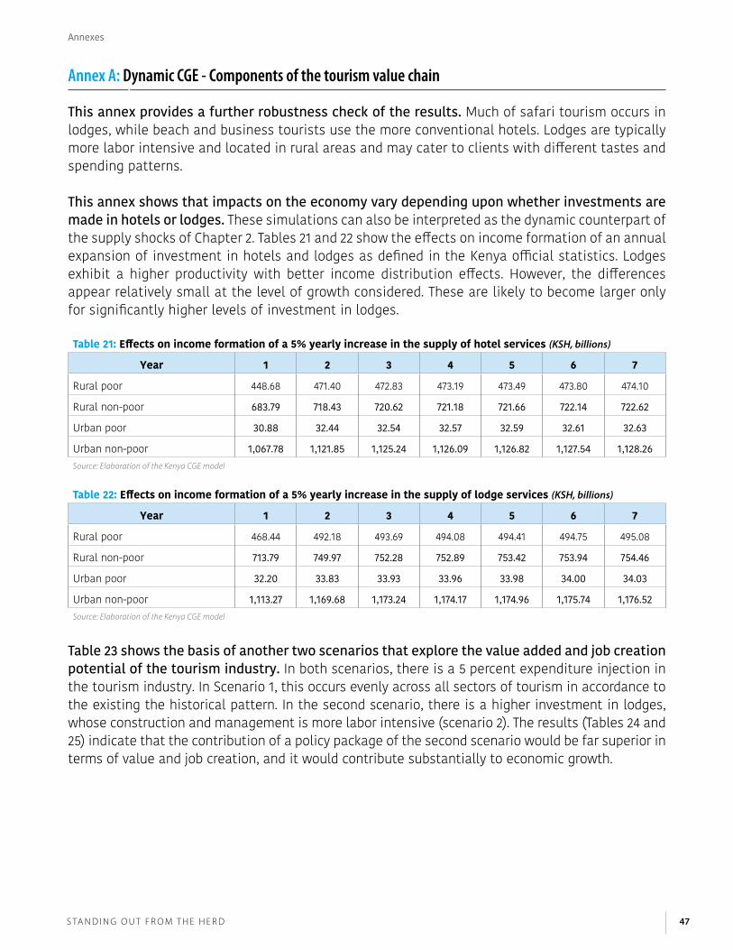
47S ta n d i n g O u t F r O m t h e h e r d
Annex A: Dynamic CGe - Components of the tourism value chain
This annex provides a further robustness check of the results. Much of safari tourism occurs in lodges, while beach and business tourists use the more conventional hotels. Lodges are typically more labor intensive and located in rural areas and may cater to clients with different tastes and spending patterns.
This annex shows that impacts on the economy vary depending upon whether investments are made in hotels or lodges. These simulations can also be interpreted as the dynamic counterpart of the supply shocks of Chapter 2. Tables 21 and 22 show the effects on income formation of an annual expansion of investment in hotels and lodges as defined in the Kenya official statistics. Lodges exhibit a higher productivity with better income distribution effects. However, the differences appear relatively small at the level of growth considered. These are likely to become larger only for significantly higher levels of investment in lodges.
Table 21: Effects on income formation of a 5% yearly increase in the supply of hotel services (KSH, billions)
Year 1 2 3 4 5 6 7
Rural poor 448.68 471.40 472.83 473.19 473.49 473.80 474.10
Rural non-poor 683.79 718.43 720.62 721.18 721.66 722.14 722.62
Urban poor 30.88 32.44 32.54 32.57 32.59 32.61 32.63
Urban non-poor 1,067.78 1,121.85 1,125.24 1,126.09 1,126.82 1,127.54 1,128.26Source: Elaboration of the Kenya CGE model
Table 23 shows the basis of another two scenarios that explore the value added and job creation potential of the tourism industry. In both scenarios, there is a 5 percent expenditure injection in the tourism industry. In Scenario 1, this occurs evenly across all sectors of tourism in accordance to the existing the historical pattern. In the second scenario, there is a higher investment in lodges, whose construction and management is more labor intensive (scenario 2). The results (Tables 24 and 25) indicate that the contribution of a policy package of the second scenario would be far superior in terms of value and job creation, and it would contribute substantially to economic growth.
Table 22: Effects on income formation of a 5% yearly increase in the supply of lodge services (KSH, billions)
Year 1 2 3 4 5 6 7
Rural poor 468.44 492.18 493.69 494.08 494.41 494.75 495.08
Rural non-poor 713.79 749.97 752.28 752.89 753.42 753.94 754.46
Urban poor 32.20 33.83 33.93 33.96 33.98 34.00 34.03
Urban non-poor 1,113.27 1,169.68 1,173.24 1,174.17 1,174.96 1,175.74 1,176.52Source: Elaboration of the Kenya CGE model
Annexes

48 E c o n o m i c A s s e s s m e n t o f To u r i s m i n K e n y a
Table 23: Alternative investment scenarios in the tourism value chain (5% increase spread over 7 years)(KSH, millions)
Scenario 1 Scenario 2
Total investment Share of total Total investment Share of total
Hotel 50,980 8.8% 51,000 8.8%
Lodge 16,448 2.8% 51,000 8.8%
Rent house 24,623 4.2% 24,623 4.2%
Restaurant 51,344 8.9% 51,344 8.9%
Transport 436,519 75.3% 401,947 69.3%
Total 579,914 100.0% 579,914 100.0%Source: Elaboration of the Kenya CGE model
Table 24: Value-added effects of scenario 1 (KSH, millions)
Year 1 2 3 4 5 6 7 8
Skilled labor 5,397 5,175 5,184 5,206 5,228 5,249 5,271 36,710
Semi-skilled labor 11,251 11,429 11,481 11,526 11,571 11,616 11,661 80,535
Unskilled labor 3,918 3,937 3,958 3,980 4,001 4,023 4,044 27,861
Capital 25,297 25,171 25,259 25,357 25,456 25,555 25,655 177,751
Land 1,002 993 1,000 1,008 1,016 1,023 1,031 7,072
Import tariffs 342 341 343 345 346 348 350 2,415
Sales taxes 3,410 3,385 3,407 3,431 3,454,89 3,479 3,503 24,072
GDP 50,619 50,431 50,632 50,852 51,073 51,294 51,515 356,416
Baseline (A)
Total Impact (over the seven year
period) (B)Ratio
(A/B) %
Skilled labor 468,237 36,710 7.84
Semi-skilled labor 1241,740 80,535 6.49
Unskilled labor 576,664 27,861 4.83
Capital 2509,569 177,751 7.08
Land 279,935 7,072 2.53
Import tariffs 52,114 2,415 4.63
Sales taxes 521,342 24,072 4.62
GDP 5649,601 356,416 6.31
Source: Elaboration of the Kenya CGE model
Annexes
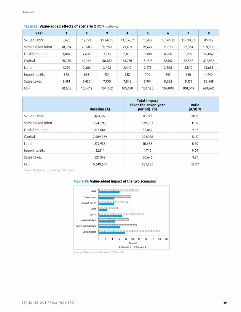
49S ta n d i n g O u t F r O m t h e h e r d
Table 25: Value-added effects of scenario 2 (KSH, millions)
Year 1 2 3 4 5 6 7 8
Skilled labor 5,693 12,793 13,242,13 13,356,37 13,452 13,546,32 13,638,83 85,722
Semi-skilled labor 10,964 20,583 21,258 21,481 21,679 21,873 22,064 139,903
Unskilled labor 3,887 7,636 7,913 8,015 8,108 8,200 8,292 52,052
Capital 25,250 49,168 50,782 51,278 51,717 52,152 52,588 332,936
Land 1,020 2,303 2,402 2,440 2,475 2,508 2,540 15,688
Import tariffs 343 698 724 732 740 747 755 4,740
Sales taxes 3,451 7,430 7,730 7,846 7,954 8,062 8,171 50,645
GDP 50,608 100,612 104,052 105,150 106,125 107,090 108,049 681,686
Baseline (A)
Total Impact (over the seven year
period) (B)Ratio
(A/B) %
Skilled labor 468,237 85,722 18.31
Semi-skilled labor 1,241,740 139,903 11.27
Unskilled labor 576,664 52,052 9.03
Capital 2,509,569 332,936 13.27
Land 279,935 15,688 5.60
Import tariffs 52,114 4,740 9.09
Sales taxes 521,342 50,645 9.71
GDP 5,649,601 681,686 12.07
Source: Elaboration of the Kenya CGE model
Figure 18: Value-added impact of the two scenarios
Source: Elaboration of the Kenya CGE model
GDP
Sales taxes
Import tariffs
Land
Capital
Unskilled labor
Semi-skilled labor
Skilled labor
Scenario 1
Percent0 2 4 6 8 10 12 14 16 18 20
Scenario 2
Annexes

50 E c o n o m i c A s s e s s m e n t o f To u r i s m i n K e n y a
This annex describes the manner in which water is integrated into the CGE model and the introduction of water into the SAM. The annex begins with a brief overview of the concepts that are relevant to exploring the effects of water in a general equilibrium context. To gain a greater understanding of the ways in which water impacts the economy, it is necessary to explore the role of water in each of the significant sectors of the economy that consume water. This is achieved by introducing water in the Social Accounting Matrix as described in the boxes below. This is followed by a description of the effects of water on the economy, beginning with the backward and forward linkages.
Annex B: Water in the CGe model
Box 3: Water in the SAM and CGE models and some crucial definitions
The incorporation of water into a SAM has traditionally been based on the idea of linking the input-output accounts with the natural system (see, for example, Isard (1969), Ayres & Kneese (1969), Daly (1968), Leontief (1970), and Victor (1972)). For water, as for other environmental goods, the methodology has followed a two stage process, consisting firstly in creating quantity based satellite accounts of the flows, and secondly integrating these flows into components of the income generation cycle by converting them into values.
The concept of Virtual Water (VW) was defined by Allan (1993, 1994) as the water embodied in a product; i.e., as the amount of water that is used to generate a given product. The Water Footprint (WF) of a sector, a region, or a country on the other hand is a closely related concept, which is defined as the volume of VW necessary for the satisfaction of one unit of final demand. The consumption pattern of different economies can thus be characterized by the direct and indirect withdrawal of water, taking into account the international water flow involved in commodity trade (Chapagain & Hoekstra (2004), Hoekstra & Hung (2002), and Hoekstra & Chapagain (2007).
In CGE models, water may be considered a factor of production (to produce something), as an intermediate input (a good not catering to final consumers), and a consumption good (caters to final demand). Furthermore, in the water geography and hydrology literature, “blue water” is defined as water extracted from aquifers, lakes and rivers, used by irrigated agriculture, and “green water” is the rainwater used by rain fed agriculture, while “grey water” is the amount of water needed to flush pollutants.
In some CGE models, water is treated only as a municipal good (Wittwer, 2009) by focusing on municipal water demands as intermediate inputs or final consumption goods where trade-offs between urban water demands and water for crop irrigation are of central concern. Treated water for urban use and untreated water for irrigation enter the production function both as an intermediate input and as a factor of production.
Annexes

51S ta n d i n g O u t F r O m t h e h e r d
Using the 2003 KIPPRA-IFPRI and the KNBS SAMs as starting points, an Environmental–Water Resources SAM is built for Kenya by applying the entropic methodology described in Scandizzo and Ferrarese (2015) to national and state account data and other statistics (Kiringai et al., 2006, KNBS a,b,c,d, 2014). These methods are based on the so called “maximum entropy econometrics” (Golan, Judge, and Miller (1996) and are able to handle the “ill-conditioned” estimation problems associated with the lack of the degrees of freedom typical of i-o matrices. The methods are very flexible in combining a variety of specific data with prior information and national accounts.
The matrix estimated contains a detailed natural resource account, including water resources, water distribution, and natural capital in various forms. The multipliers of this chapter correspond to the hypothesis that the rest of the world (including international tourists), investment, and the government are exogenous. Under this hypothesis, backward multipliers are on average 0.13, between a minimum of 0.06 for machinery to a maximum of more than 0.22 for distribution water, and highs of around 0.12-0.16 for agriculture, tourism, and most services.
For water, in particular, it turns out that for both blue and green water, backward multipliers are very high at about 0.237, or almost twice the average backward multiplier of the other sectors. This means that on average an increase in 1% of demand for water is met with a 0.237% increase in the demand for inputs from other sectors. Forward multipliers are also similar for blue and green water and are around 0.09, which is about 72% of the average forward multiplier. This implies a much weaker linkage of water with the sectors that are closer to the final consumer, with only a 0.09% of increase in water demand in response to an average 1% increase in all other sectors of the economy.
Natural resources usually have higher backward than forward multipliers as a consequence of the lower contribution to sector uses compared to their response to exogenous demand increases in terms of demand for conservation, renewal, and management.
Annexes

52 E c o n o m i c A s s e s s m e n t o f To u r i s m i n K e n y a
Annex C: Water estimates
Table 26: Kenya SAM—Backward and forward multipliers
Multiplier impacts of water
Forward multipliers Backward multipliers
Mean Rasmussen Mean Rasmussen
Skilled labor 0.210 1.602 0.170 1.297
Semi-skilled labor 0.477 3.642 0.170 1.301
Unskilled labor 0.175 1.335 0.165 1.269
Capital 0.862 6.581 0.114 0.886
Land 0.124 0.948 0.180 1.392
Blue water 0.093 0.714 0.237 1.842
Green water 0.094 0.720 0.237 1.869
Non-renewable natural resources 0.016 0.125 0.166 1.326
Water resources 0.203 1.551 0.221 1.784
Savanna and forest habitat 0.044 0.335 0.099 0.805
Emissions 0.020 0.156 0.015 0.125
Natural capital 0.028 0.211 0.114 0.913
Rural poor 0.276 2.105 0.167 1.339
Rural non-poor 0.422 3.221 0.165 1.330
Urban poor 0.039 0.296 0.167 1.356
Urban non-poor 0.834 6.368 0.142 1.160
Domestic tourist 0.051 0.391 0.146 1.193
Enterprise 0.864 6.594 0.101 0.831
Direct taxes 0.127 0.970 0.015 0.126
Import tariffs 0.035 0.269 0.015 0.124
Sales taxes 0.227 1.732 0.015 0.121
Irrigated agriculture (international) 0.094 0.721 0.168 1.297
Non irrigated agriculture (international) 0.113 0.859 0.170 1.323
Mining (international) 0.029 0.218 0.142 1.114
Food, beverage & tobacco (international) 0.037 0.282 0.111 0.875
Petroleum (international) 0.018 0.139 0.112 0.878
Textile & clothing (international) 0.019 0.146 0.112 0.873
Leather & footwear (international) 0.019 0.143 0.129 1.006
Printing & publishing (international) 0.020 0.152 0.067 0.524
Chemicals (international) 0.023 0.178 0.074 0.571
Metals & machines (international) 0.018 0.136 0.065 0.497
Non-metallic products (international) 0.016 0.122 0.144 1.076
Other manufactures (international) 0.026 0.202 0.121 0.905
Annexes

53S ta n d i n g O u t F r O m t h e h e r d
Multiplier impacts of water
Forward multipliers Backward multipliers
Mean Rasmussen Mean Rasmussen
Irrigated agriculture 0.047 0.356 0.168 1.258
Non-irrigated agriculture 0.494 3.768 0.170 1.285
Forestry & fishing 0.044 0.335 0.142 1.078
Poaching 0.016 0.122 0.142 1.083
Mining 0.029 0.224 0.145 1.107
Food, beverage & tobacco 0.227 1.730 0.112 0.862
Petroleum 0.041 0.313 0.112 0.857
Textile & clothing 0.040 0.305 0.112 0.850
Leather & footwear 0.021 0.164 0.129 0.976
Wood & paper 0.050 0.385 0.101 0.763
Printing & publishing 0.093 0.710 0.067 0.504
Chemicals 0.092 0.702 0.075 0.544
Metals & machines 0.041 0.315 0.065 0.467
Non-metallic products 0.025 0.191 0.149 1.036
Other manufactures 0.100 0.763 0.121 0.839
Distribution water 0.059 0.449 0.228 1.568
Electricity 0.075 0.570 0.130 0.929
Construction 0.021 0.159 0.130 0.927
Trade 0.296 2.258 0.143 1.010
Hotel 0.024 0.180 0.125 0.885
Lodge 0.018 0.138 0.124 0.872
Rent House 0.019 0.147 0.125 0.866
Restaurant 0.024 0.180 0.128 0.873
Transport 0.264 2.018 0.138 0.927
Information & communication 0.102 0.776 0.149 0.996
Financial & insurance activities 0.176 1.346 0.141 0.942
Real estate 0.151 1.156 0.149 0.987
Other services 0.101 0.772 0.147 0.967
Public administration & defence 0.036 0.271 0.137 0.897
Health & social work 0.041 0.316 0.161 1.020
Education 0.079 0.600 0.159 1.016
Package 0.015 0.117 0.154 1.000
Average production activities 0.075 1.000 0.129 1.000
Source: Elaboration of the Kenya CGE model
Annexes

54 E c o n o m i c A s s e s s m e n t o f To u r i s m i n K e n y a
Annex D: The water footprint
Using historical data on national accounts and data from a plurality of sources, we have estimated the SAM accounts for water. Table 27 below contains the results of the SAM estimates of water withdrawn directly and indirectly by each sector. These values measure the amount of water directly and indirectly withdrawn to sustain the final demand of the sector and, as relative indicators, the ratio between the water value and the sector final demand value (value ratio) and the water quantity and the final consumption value (quantity to value ratio). They can be therefore interpreted as indicators of the water footprints of each sector. As the comparison of figures shows, the apparent domination of the irrigated agricultural sector in terms of direct water withdrawals is mitigated by this water footprint measure.
When both direct and direct withdrawals are taken into account, several counterintuitive results follow: (i) traditional agriculture and mining are more water intensive than irrigated agriculture; and (ii) industrial sectors and services are less water intensive in terms of value to production ratio than services. We believe these results are new and highlight the importance of taking into account feedback effects when considering the footprint an economic activity. Stated simply, a sector that consumes less water than another may stimulate other more water-intensive types of economic activity that end up consuming a larger amount of water. This is why non-irrigated agriculture and mining have a larger water footprint than irrigated agriculture.
Table 27: Water footprint (direct and indirect use of water resources)
KSH, million
Value ratio (water as %
of production value) Million m3
Quantity to Value Ratio
(m3/US$)
Total Production
Value (KSH, million)
Irrigated agriculture 28,874.64 36.30 2,887.46 3.630 79,539.40
Non-irrigated agriculture 114,792.08 8.18 114,792.08 8.178 1,403,673.04
Industry 34,792.11 3.01 1,739.61 0.150 1,157,489.14
Services 153,154.12 4.50 5,105.14 0.150 3,406,984.85
Mining 2,679.06 6.45 2,679.06 6.451 41,529.19
Figure 19: Water footprint
Source:
Irrigatedagriculture
Non-irrigatedagriculture
Industry
Value ratio M2/US$
Services Mining
40
35
30
25
20
15
5
0
Annexes

55S ta n d i n g O u t F r O m t h e h e r d
Annex e: sAm water accounts showing the use of different types of water by sector
Table 28: Water use by sector
Irrigated agriculture
Non-irrigated agriculture
Forestry & fishing Wildlife Mining
KSH, millions
Blue water 17,323.29 0 0.00 319.25 292.76
Green water 0 17,986.75 61.35 0.00 0.00
Distribution water 60.76 891.22 0.00 0.00 68.02
Million Cubic Meters
Blue water 2,000.00 0 0 319.25 292.76
Green water 0 18,700.00 61.35 0 0
Distribution water 6.76 89.12 0 0 68.02
Table 29: Gross incomes by natural resource sectors (KSH, millions)
Blue water Green waterNon-renewable
natural resources Water resources
Blue water 0.00 0.00 778.87 23,615.73
Green water 0.00 0.00 0.00 28,615.83
Water resources 57,081.00 71,620.86 0.00 0.00
Distribution water 0.00 0.00 0.00 21,821.32
Total 57.081.00 71.620.86 778.87 74,052.88
Table 30: Effects of water use on gross incomes by sector (KSH, millions)
Rural poor Rural non-poor Urban poorUrban
non-poor Government
Blue water 297.60 379.45 30.91 0.00 0.00
Green water 869.27 76.87 0.00 0.00 0.00
Water resources 0.00 0.00 0.00 0.00 0.00
Distribution water 0.00 224.24 0.00 5,924.04 1.141.90
Total 1.166.86 680.56 30.91 5,924.04 1.141.90
Annexes
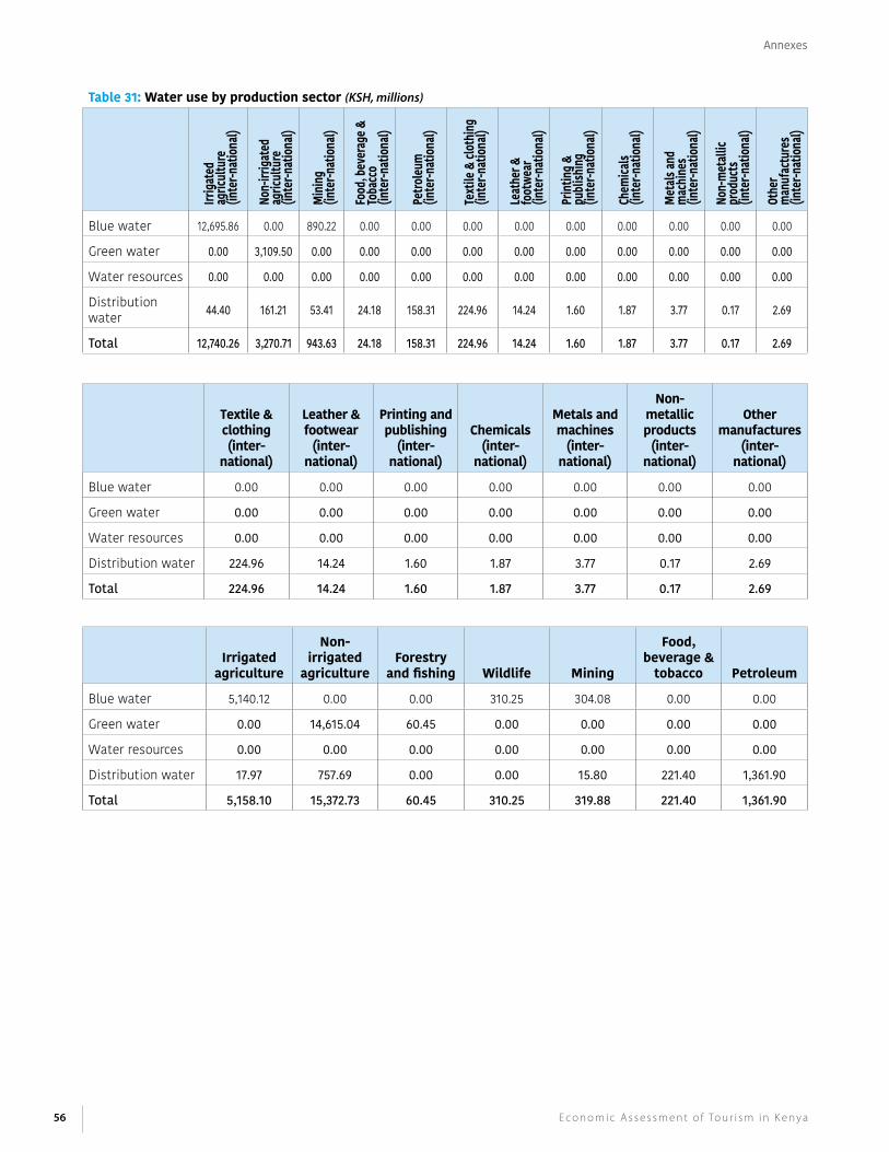
56 E c o n o m i c A s s e s s m e n t o f To u r i s m i n K e n y a
Table 31: Water use by production sector (KSH, millions)
Irrig
ated
ag
ricul
ture
(in
ter-n
atio
nal)
Non-
irrig
ated
ag
ricul
ture
(in
ter-n
atio
nal)
Min
ing
(inte
r-nat
iona
l)
Food
, bev
erag
e &
Toba
cco
(inte
r-nat
iona
l)
Petro
leum
(in
ter-n
atio
nal)
Text
ile &
clot
hing
(in
ter-n
atio
nal)
Leat
her &
fo
otw
ear
(inte
r-nat
iona
l)
Prin
ting
& pu
blish
ing
(inte
r-nat
iona
l)
Chem
icals
(inte
r-nat
iona
l)
Met
als a
nd
mac
hine
s (in
ter-n
atio
nal)
Non-
met
allic
pr
oduc
ts
(inte
r-nat
iona
l)
Othe
r m
anuf
actu
res
(inte
r-nat
iona
l)
Blue water 12,695.86 0.00 890.22 0.00 0.00 0.00 0.00 0.00 0.00 0.00 0.00 0.00
Green water 0.00 3,109.50 0.00 0.00 0.00 0.00 0.00 0.00 0.00 0.00 0.00 0.00
Water resources 0.00 0.00 0.00 0.00 0.00 0.00 0.00 0.00 0.00 0.00 0.00 0.00
Distribution water 44.40 161.21 53.41 24.18 158.31 224.96 14.24 1.60 1.87 3.77 0.17 2.69
Total 12,740.26 3,270.71 943.63 24.18 158.31 224.96 14.24 1.60 1.87 3.77 0.17 2.69
Textile & clothing (inter-
national)
Leather & footwear
(inter-national)
Printing and publishing
(inter-national)
Chemicals (inter-
national)
Metals and machines
(inter-national)
Non-metallic products
(inter-national)
Other manufactures
(inter-national)
Blue water 0.00 0.00 0.00 0.00 0.00 0.00 0.00
Green water 0.00 0.00 0.00 0.00 0.00 0.00 0.00
Water resources 0.00 0.00 0.00 0.00 0.00 0.00 0.00
Distribution water 224.96 14.24 1.60 1.87 3.77 0.17 2.69
Total 224.96 14.24 1.60 1.87 3.77 0.17 2.69
Irrigated agriculture
Non-irrigated
agricultureForestry
and fishing Wildlife Mining
Food, beverage &
tobacco Petroleum
Blue water 5,140.12 0.00 0.00 310.25 304.08 0.00 0.00
Green water 0.00 14,615.04 60.45 0.00 0.00 0.00 0.00
Water resources 0.00 0.00 0.00 0.00 0.00 0.00 0.00
Distribution water 17.97 757.69 0.00 0.00 15.80 221.40 1,361.90
Total 5,158.10 15,372.73 60.45 310.25 319.88 221.40 1,361.90
Annexes

57S ta n d i n g O u t F r O m t h e h e r d
Textile & clothing
Leather & footwear
Wood & paper
Printing & publishing Chemicals
Metals & machines
Non-metallic products
Other man-ufactures
Blue water 0.00 0.00 0.00 0.00 0.00 0.00 0.00 0.00
Green water 0.00 0.00 0.00 0.00 0.00 0.00 0.00 0.00
Water resources 0.00 0.00 0.00 0.00 0.00 0.00 0.00 0.00
Distribution water 1,402.51 23.49 184.57 25.69 16.47 39.87 1.67 29.02
Total 1,402.51 23.49 184.57 25.69 16.47 39.87 1.67 29.02
Distri-bution water Electricity
Construc-tion Trade Hotel Lodge
Rent House
Restau-rant
Blue water 12,637.91 0.00 0.00 0.00 0.00 0.00 0.00 0.00
Green water 19,828.26 0.00 0.00 0.00 0.00 0.00 0.00 0.00
Water resources 0.00 0.00 0.00 0.00 0.00 0.00 0.00 0.00
Distribution water 1,253.49 56.84 265.23 384.11 72.47 25.37 36.51 73.41
Total 33,719.66 56.84 265.23 384.11 72.47 25.37 36.51 73.41
Transport
Informa-tion &
communi-cation
Finan-cial and
insurance activities
Real es-tate
Other services
Public ad-ministra-tion and defence
Health & social
work Education
Blue water 0.00 0.00 0.00 0.00 0.00 0.00 0.00 0.00
Green water 0.00 0.00 0.00 0.00 0.00 0.00 0.00 0.00
Water resources 0.00 0.00 0.00 0.00 0.00 0.00 0.00 0.00
Distribution water 92.85 1,033.06 254.88 82.61 480.05 1,205.00 1,871.28 1,803.27
Total 92.85 1,033.06 254.88 82.61 480.05 1,205.00 1,871.28 1,803.27
Packagetourism
Business tourism (international)
Beach tourism (international)
Safari tourism (international)
Other tourism (international)
Blue water 0.00 0.00 0.00 0.00 0.00
Green water 0.00 0.00 0.00 4.445.63 0.00
Water resources 0.00 0.00 0.00 0.00 0.00
Distribution water 43.69 175.88 86.51 258.28 52.37
Total 43.69 175.88 86.51 4,703.91 52.37
Annexes

58 E c o n o m i c A s s e s s m e n t o f To u r i s m i n K e n y a
Annex F: effects of water transfer to tourism
Table 32: Impact of a 20% water transfer from irrigated agriculture to hotels and lodges (KSH, millions)
Impact (A) Baseline (B) Ratio (A/B) %
Irrigated agriculture -91,237.86 133,853 -68.16
Non-irrigated agriculture 116,245.10 11,553,870 7.48
Forestry & fishing 9,947.62 84,187 11.82
Wildlife 255.18 1,896 13.46
Mining 18,766.77 172,713 10.87
Food, beverage & tobacco 64,240.14 441,772 14.54
Petroleum 3,281.00 53,597 6.12
Textile & clothing 5,628.61 50,280 11.19
Leather & footwear 3,146.15 34,891 9.02
Wood & paper 8,689.17 58,116 14.95
Printing and publishing 19,639.76 137,929 14.24
Chemicals 11,684.12 101,682 11.49
Metals and machines 10,592.84 100,782 10.51
Non-metallic products 10,614.65 101,621 10.45
Other manufactures 29,392.07 239,183 12.29
Distribution water -557.68 43,508 -1.28
Electricity 70,668.34 176,434 40.05
Construction 64,852.27 683,530 9.49
Trade 144,154.65 769,114 18.74
Hotel 312,186.69 39,053 799.40
Lodge 281,785.01 12,373 2277.38
Rent House 1,181.85 18,606 6.35
Restaurant 2,521.94 39,577 6.37
Transport 63,911.52 773,604 8.26
Information & communication 37,357.19 259,815 14.38
Financial & insurance activities 92,556.40 459,857 20.13
Real estate 50,924.71 452,791 11.25
Other services 27,878.44 251,935 11.07
Public administration & defence 45,260.45 411,537 11.00
Health & social work 11,706.32 160,127 7.31
Education 26,254.30 479,733 5.47
Package 3,966.61 33,230 11.94
Total 1,276,616 5,405,625 23.62
Source: Elaboration of the Kenya CGE model
Annexes
59S ta n d i n g O u t F r O m t h e h e r d
Allan, J. A. (1994). “Overall perspectives on countries and regions.” In Water in the Arab World: Perspectives and Prognoses, ed. Rogers, P., and P. Lydon. Harvard University Press, Cambridge. Massachusetts.
Ayres, R.U., and A.V. Kneese. (1969). “Production, consumption and externalities.” American Economic Review (59): 282–297.
Berck, P.S. Robinson, and G. Goldman. (1991). “The Use of Computable General Equilibrium Models to Assess Water Policies.” In The Economics and Management of Water and Drainage in Agriculture, ed. Berck. P. S. Robinson, and G. Goldman, 489-509. Norwell. MA: Kluwer Academic Publishing.
Blien, U., and F. Graef. (1992). “ENTROP: A General Purpose Entropy Optimizing Method for the Estimation of Tables: The Weighting of Samples, the Disaggregation of Data, and the Development of Forecasts.”
Chapagain, A. K., and A.Y Hoekstra. (2004). “Water footprints of nations.” Value of Water Research Report Series No. 16. UNESCO-IHE Delft, The Netherlands.
Christie, L.E. Fernandes, H. Messerli, and L. Twining Ward. (2013). “Tourism in Africa: Harnessing Tourism for Growth and Improved Livelihoods.” The World Bank, Washington DC.
Daly, H.E. (1968). “On economics as life science.” The Journal of Political Economy 76 (3): pp. 392–406.
Dixon, P. B. (1990). “A General Equilibrium Approach to Public Utility Pricing: Determining Prices for a Water Authority.” Journal of Policy Modeling, 12(4): pp. 745-67.
Fadali, E., K. Rollins, and S. Stoddard. (2013). “Determining Water Values with Computable General Equilibrium Models.” Industrial Economics. Inc.
FAO. (2014). “FAOSTAT, Acquastat database for Kenya.”
Golan, A., G. Judge, and D. Miller. (1996). “Maximum Entropy Econometrics: Robust Estimation With Limited Data.” Chichester etc., Wiley.
Goodman, D.J. (2000). “More Reservoirs or Transfers? A Computable General Equilibrium Analysis of Projected Water Shortages in the Arkansas River Basin.” Journal of Agricultural and Resource Economics. 25(2): pp. 698-713.
Haberman, S.J. (1984). “Adjustment by minimum discriminant information.” The Annals of Statistics. 12/3, 971.
Harris, R. L. (2002). “Estimation of a regionalized Mexican Social Accounting Matrix.” TMD discussion papers 97. International Food Policy Research Institute (IFPRI).
Hoekstra, A., and A.K. Chapagain. (2007). “Water footprints of nations: Water use by people as a function of their consumption pattern.” Water Resources Management 21(1): 35-48.
Hoekstra, A.Y., and P.Q Chung. (2002). “Virtual water trade: a quantification of virtual water flows between nations in relation to international crop trade.” Value of Water Research Report Series No.11, IHE Delft.
reFerenCes

60 E c o n o m i c A s s e s s m e n t o f To u r i s m i n K e n y a
Horridge, M., P.B. Dixon, and M.T Rimmer. (1993). “Water Pricing and Investment in Melbourne: General Equilibrium Analysis with Uncertain Streamflow.” Centre of Policy Studies, Monash University.
Isard, W. (1969). General Theory: Social, political, economic, and regional, with particular reference to decision-making analysis. Cambridge: M.I.T Press.
Isard, W. (1969). “Some notes on the linkage of ecologic and economic systems.” Regional Science 22: pp. 85–96.
Kiringai, J., J. Thurlow, and B. Wanjala. (2006). “A 2003 Social Accounting Matrix (SAM) for Kenya.” Kenya Institute for Public Policy Research and Analysis, Nairobi, and International Food Policy Research Institute, Washington. D.C.
KNBS (Kenya National Bureau of Statistics). (2016). “Economic Survey 2016.”
KNBS. (2014a). “Gross Domestic Product by sectors.”
KNBS. (2014b). “Visitors Statistics.”
KNBS. (2014c). “Wage Employment by Industry.”
KNBS. (2014d). “Information on the Revised National Accounts.”
Leontief, W. (1970). “Environmental Repercussions and the Economic Structure: An Input-Output Approach.” Review of Economic Statistics. Vol.52: pp.262-277.
Letsoalo, A.T., et al. (2007). “Triple Dividends of Water Consumption Charges in South Africa.” Water Resources Research 43(5).
Ministry of Land, Housing and Urban Development. (2014). “Kenya National Housing Survey. 2012-2013.”
Oxford Business Group. (2016). The Report: Kenya 2016.
Robinson, S., and C. Gehlar. (1995). “Land, Water, and Agriculture in Egypt: The Economywide Impact of Policy Reform.” In TMD Discussion Paper No. 1. 1-50, Washington, D.C.: International Food Policy Research Institute.
Roson, R., and M. Sartori. (2010). “Water Scarcity and Virtual Water Trade in the Mediterranean.” Working Paper, Department of Economics Ca’ Foscari University, Venice, Italy.
Scandizzo, P.L., and C. Ferrarese. (2015). “Social Accounting Matrix: A new estimation methodology.” Journal of Policy Modeling 37 (1): pp. 14–34.
Scandizzo, P.L., and C. Ferrarese. (2015). “A CGE Model for Tanzania.” Technical Report. The World Bank.
Smith, C.A., A.J. Simon, and R.D. Belles. (2011). “Estimated Water Flows in 2005.” Livermore. CA: Retrieved from https://flowcharts.llnl.gov/.
Seung, C., J. Englin, and T. Harris. (1997). “Application of Computable General Equilibrium Model to Derive Impacts of Surface Water Reallocation Policy.” Journal of Agricultural and Resource Economics. 22(2): pp. 395-95.
References

61S ta n d i n g O u t F r O m t h e h e r d
Seung, C., T. Harris, and R. Narayanan. (1998). “A Computable General Equilibrium Approach to Surface Water Reallocation Policy in Rural Nevada.” American Journal of Agricultural Economics 80(5).
Seung, C., T. Harris, J. Englin, and N.R. Netusil. (2000). “Impacts of Water Reallocation: A Combined Computable General Equilibrium and Recreation Demand Model Approach.” Annals of Regional Science. 34(4): pp. 473-87.
Stone, R.N. (1962). “Multiple classifications in social accounting.” Bulletin de l’Institut International de Statistique 39 (3).
Stone, R.N. (1981). “The Relationship of Demographic Accounts to National Income and Product Accounts.”
UNEP and KFS. (2012). The Role and Contribution of Montane Forests and Related Ecosystem Services to the Kenyan Economy.
United Nations. “National Systems Accounting (SCN93).” New York.
United Nations. (2003). “Integrated environmental and economic accounting 2003.” Series F, No. 61, Rev 1.
Usami, Y. (2008). “A Note on Construction of a Regional Social Accounting Matrix with natural resource accounts: Linking Village/Industry Level Data to Regional Level Studies.” Osaka Prefecture University.
Uwakonye, M.N., G.S. Osho, and E.I.S. Ajuzie. (2010). “The Economic Impact Of Water Resource: Broken Bow Lake In Mccurtain County In Southeastern Oklahoma.” Journal of Business & Economics Research 8(46).
Victor, P. A. (1972). Pollution: Economy and Environment. London: George Allen and Unwin Ltd.
Watson, P. S., and S.D. Davies. (2011). “Modeling the Effects of Population Growth on Water Resources: A CGE Analysis of the South Platte River Basin in Colorado.” Annals of Regional Science 46(2): pp. 331-48.
Wilson, A. (1970). Entropy in Urban and Regional Modeling. London: Pion Ltd.
Wittwer, G. (2006). “Modelling Future Urban and Rural Water Requirements in a CGE Framework.” Centre of Policy Studies, Monash University.
World Bank. (2016). Tanzania’s Tourism Futures: Harnessing Natural Assets.
World Bank. (2010). Kenya’s Tourism: Polishing the Jewel.
World Travel & Tourism Council. (2016). “Travel & Tourism Economic Impact 2016, Kenya.”
World Travel & Tourism Council. (2016). “Travel & Tourism Economic Impact 2016, Tanzania.”
References

Delta Center, Menengai Road, Upper HillP. O. Box 30577 – 00100 Nairobi, KenyaTelephone: +254 20 293 7706www.worldbank.org