An Econometric Analysis Of the Determinants of

JOHANNES KEPLER

UNIVERSITY LINZ

Altenberger Straße 69

4040 Linz, Osterreich

www.jku.at

DVR 0093696

Submission by Yaya Idris, BSc. Submission at Department of Economics Supervisor Dr. Jochen Güntner July 2021

An Econometric Analysis

Of the Determinants of

the iReal Exchange Rate

in Nigeria

Master’s Thesis

to obtain the academic degree of

Master of Science

in the Master’s Program

Economics

ii

Abstract

This thesis undertakes anieconometric analysis ofideterminants of theireal exchange irate in

iNigeria employingiannual dataifrom 1981 to 2019. The virtualideterminants of itheireal iexchange

irate are identified resting on existing literature, namely theinominal exchange irate,imoney supply,

iinflation rate, real GDP, iforeign reserves, openness,iglobal oil price, external debt, and

igovernment expenditure. iThe time seriesiproperties were itested using theiADF and PP unit roots

itests of stationarity.iThe variables areitested foricointegration, andirelationship coefficients were

estimated using aniAutoregressive DistributediLag (ARDL)iapproach and ErroriCorrection Model

i(ECM). Empirical results confirmed that the inominal exchange irate, inflation irate, and real iGDP

are positivelyiand significantly related to theireal exchange irate. Atithe same time, ithe money

supply,iforeign reserves, andiexternal debt are negatively and significantly related to theireal

exchange irate in Nigeria.iThe thesis alsoifound that moneyisupply and global oil price have lagged

cumulative effects onithe realiexchange rate in Nigeria. It is,itherefore, recommendedithat the

icentral authority ishould try to control the macroeconomic variables that directlyiinfluence the real

iexchange rateifluctuation andiinstitute the ilimit withiniwhich the iexchange rate canifluctuate in

iNigeria.

iii

Statutory Declaration

I hereby declare that the thesis submitted is my own unaided work, that I have not used other than

the sources indicated, and that all direct and indirect sources are acknowledged as references.

This printed thesis is identical with the electronic version submitted.

Linz, July 2021

Place, Date

Yaya Idris, BSc.

iv

Acknowledgement

My profound gratitude goes to my Supervisor Dr. Jochen Güntner for his support, helpful

comments, and guidance at every stage of this thesis. He supervised this thesis diligently,

exceptionally patient with me and inspiring me a lot. Thank you for everything Prof!

I am grateful to the coordinators of the master thesis seminar: Dr. Martin Halla and Dr. Rene

Böheim for itheir valuable icomments and input idiscussions. The roles of all staff and course mates

in the department of Economics, University of Linz, are also acknowledged.

Many thanks to my family and friends who have shown great interest in my academic, and for their

moral support and encouragement.

Above all, I give all glory and honor to Almighty God for life, grace and favor granted to me.

v

Contents

1 Introduction 8

2 Literature Review 10

2.1 iExchange Rate iPolicy in Nigeria ……………………………………………….11

2.2 Theoretical Framework ………………………………………………………….22

2.3 Empirical Review ………………………………………………………………..28

3 Data Description 30

3.1 Data Sources ……….……………………………………………………………30

3.2 Definition of Variables ………………………………………………………….31

3.3 Unit Root Test ….……………………………………………………………….32

4 Methodology 34

4.1 Log Linear/Model Specification ..……………………………………………….34

4.2 ARDL Model Specification …...………………………………………...............35

4.3 ECM Model ….………………………………………………………………….36

5 Empirical Results 37

5.1 Cointegration Test ……………………………………………………………....37

5.2 Short-run Aspect of iReal Exchange iRate in Nigeria…………………………....39

5.3 Diagnostic Test …………………………………………………………………..42

6 Conclusion and Policy Recommendations 43

7 References 46

vi

List of Tables

1. Arrangement of Events iniExchange RateiManagementiin Nigeria …………………….17

2. Naira Exchange Rate Movementiin the ForeigniExchange Market………….…………..20

3. Definitions and Sources of Variables ..…………………………………………………..31

4. Stationarity Test of the Variables (ADF test and PP test) ……………………………….32

5. Results of BoundsiTest for Cointegration …………………………………………….38

6. Estimated Long iRun Coefficients using iARDL Approach …………………………...39

7. Error iCorrection Model iRepresentation for the iSelected ARDL Model …………..…..40

8. Diagnostic Tests for Underlying ARDL (1 1 2 1 0 1 2 0 1 1) Model …………………....42

List of Figures

1. Nominal Bilateral Exchange Rate of Nigeria Naira against US Dollar …..……………..18

2. Real Bilateral Exchange Rate of Nigeria Naira against US Dollar….…………………...19

3. Monthly Fluctuation in Exchange Rate over time………………………...……………...19

4. Plot of CUSUM Test for Coefficients Stability of ARDL Model………...……………...42

5. Plot of CUSUMSQ Test for Coefficients Stability of ARDL Model…..………………...43

8

1. Introductioni

Theireal exchangeirate has resulted in uncertainty in achieving macroeconomic objectives in many

economies globally, both in developed and developing countries. Unstable real exchange rates lead

to fluctuations in short-term capital flows, which subsequently affect Central Bank’s net foreign

assets. From a policy descriptive standpoint, the exchange rate is essentially related with the

economic growth. The ireal exchange irate is critical in controlling the home economy's broad

distribution of production and consumption between foreign andi domestic goods. (Oriavwote iand

Oyovwi, 2012).

The realiexchange rate is definedias the nominaliexchange rate that takes the inflation idifferentials

among countries into account. In the long run, it is defined as nominal exchange rate that is

adjusted by the iratio of the foreign iprice level to the domestic iprice level. Theidecline in theireal

exchange irate can be represented as the realiappreciation of theiexchange rate (Ahmet and

Mehtap, 1997). While the nominaliexchange rate indicates theivalue of a local currency initerms

of foreign money, the realiexchange rateiis a crucial relativeiprice thatidetermines trading

countries'iinternational competitiveness.

The exchange rate variability has long been a contentious topic in both theory and practice. One

of the remaining difficulties to be tackled is toiinvestigate theideterminants of theiequilibrium real

iexchange rate. The breakup of the Bretton-Wood system in 1970s caused many countries'

currency rates to fluctuate. As a result, economists and policymakers continue to concentrate their

efforts on empirical studies of exchange rates. The quest to know what can be done to limit the

fluctuation in the values of currencies has been the major challenge for policymakers across the

9

world. What factors determined the instability in the real currency values has been the significant

policy issue, and how it can be predicted has been the reasons for extensive empirical research

since the 1970s. Important advances in econometrics, combined with the growing availability of

high-quality data, have sparked a flood of empirical work on the exchange rate (Ajao and Igbekoyi,

2013).

So far, the research efforts imade by numerous researchers ito understand the ibehavior of

exchange irate have imet with only ilimited success. Because the equilibrium level of the currency

rate is not easily observable, the concept of currency fluctuations remains subjective. The question

of what brings about equilibrium level of exchange rate does not have a straightforward answer.

The most difficult empirical problem in macroeconomics is measuring theidegree ofiexchange

irate variability. The monetary authorities do not have absolute control over the changes of theireal

exchange rate. Only certain events, such asiforeign capital movement,iincreased productivity

owing to technical innovation, and changes in trade conditions, among other fundamentals, drive

changesiin the realiexchange rate (Ajao and Igbekoyi, 2013). According to the literature, real

exchange rate depreciation may have an unanticipated negative impact on the international trade

balance. Exchange rate depreciation and demand management strategies would be required to

effectively rectify the foreign disequilibrium balance.

In Nigeria, theiexchange rateiis a vital indicator. Its traditional role in the monetary policy

formulation is necessary because Nigeria is an import-dependent developing nation. Nigeria's main

monetary authority has used a variety of exchange rate measures to attain its price stability goal

on many times. The effectiveness of these policies, however, has remained a question mark. The

problem confronting the iexchange rate imanagement in Nigeria is still the inability toidetermine

10

the precise Naira iexchange rate, which iwould ensure ithe attainment iof domestic and external

balances simultaneously onia sustainableibasis. Despite various steps by the government to

maintain exchange rate constancy,ithe nairaiexchange rateito the US dollar depreciated throughout

the 1980s (Oriavwote and Oyovwi, 2012). The decline in foreign reserves, speculators' activities,

the recent economic meltdown, weak non-oil export earnings, oil earnings fluctuation, unguided

trade liberation policies, and expansionary economic policies, along with other factors, have all

been ascribed to the continuous decline in the value of the Naira.

This thesis investigates the factors that impact Nigeria’s real exchange rate, focusing on the years

1981 to 2019. The major goal of this thesis is just to present a model for determining ireal exchange

irates in Nigeria and to explore the influence of changes in likely macro - economic drivers of ithe

exchange rates. Other than this introductory section, the rest of this thesis is divided into five

sections. The first focused on a literature review, which comprises empirical literature, theoretical

literature, and institutional framework. The second deals with data description and variables

definition and construction, while the third is on methodology and model specifications. The fourth

focuses on the results and discussion of findings, including diagnostic tests. The last but not the

least section deals with the conclusion and policy recommendations of the thesis.

2. Literature Review

Several studies have been advanced to describe the fundamental determinants of real exchange in

the past. In Nigeria precisely, several empirical works have been undertaken to identify the

possible sources of real exchange rate fluctuation. Thisichapter examines relevant literature on the

iexchange rate policy, strategies, and management iniNigeria and reviewsithe empirical literature

11

on theireal exchange rate. The empirical literature would be divided into theoretical review and

empirical review accordingly.

2.1 Exchange Rate Policy in Nigeria

Many countries whose currencies do not serve as international currencies need to accumulate

foreign exchange through various means to import goods and services, which are primarily

required to promote growth and development. Nigeria falls into this category of countries, as its

currency cannot easily be converted and, as a result, must necessarily earn foreign exchange via

export, investment, or foreign loans to promote growth and towards enhancing the welfare of the

citizens. Therefore, the foreign exchange becomes a crucial resource to manage macroeconomic

stability and avoid external reserve problems efficiently.

One of the goals of public policy in Nigeria is to strengthen the currency rate, which is an important

system for controlling foreign reserves. To put it another way, any country's foreign currency

market is managed under the framework of a foreign exchange policy, “which according to

Obaseki (2001), is the total of the institutional framework and measures maintained to stabilize

the exchange rate towards its desired level to stimulate the productive sectors, ensure internal

balance, curtail inflation, improve the level of exports, and attract direct foreign investment and

other capital inflows” (Oladapo and Oloyede, 2014). The excessive volatility, ireal exchange irate

overvaluation, and the desire for aimechanism forimarket-determined rates whereithe

governmentiis the exclusive source of foreign exchange are the most important arguments that

emergeiin theidiscussion ofiexchange rates and administration in Nigeria. (Ajao & Igbekoyi 2013).

12

Nigeria has implemented several exchange rate regimes which can divided into a distinct period

of the formally pegged system between 1970 and 1985 to a flexible system under SAP (Structural

Adjustment Program) in 1986 and the period after SAP with lots of mixed methods of the exchange

rate. Within the following time frames, the evolution and pattern of currency rate control in Nigeria

can be examined.

The 1960-1986 Period

Theifounding of theiCentral Bank ofiNigeria in 1959 was the first step toward managing Nigeria's

currency rate. The CBN was created with the purpose of managing the country's currency to

achieve stable national currency. The Nigerian Pound was maintained at par with the pound

sterling by the Central Bank Ordinance of 1959, and the CBN was given authority for buying and

selling foreign currency in Nigeria. The exchange irate policy's specific aims during that time were

to equilibrate the ibalance of ipayments and maintain ithe value of external ireserves. Maintaining

a steady exchange rate was especially important at early stage after the independence, as a result

the Nigerian Naira was set at one to one with the British Pound.

Another fixed parity with the US Dollar was maintained until 1974, when it was replaced in 1976

by an independent exchange rate management policy that tied the Naira to either the US dollar or

the British pound sterling. A policy of stable Naira appreciation was implemented during this time.

Nigeria consistently ran considerable external surpluses in the balance of payments over the

period, which supported the Naira's appreciation. Due to the shifting prospects of Nigeria's

economic situation in the later half of 1976, a policy reversal in regulating the naira exchange rate

was implemented. The degree of exchange control was reduced in 1981, owing mostly to a better

13

balance of payments because of good developments in the global oil market. The final phase of

Nigeria's currency rate control regime was from 1982 to 1985. Export receipts were regularly fewer

than import settlements in foreign exchange. Due to the necessary reliance on short-term external

loans to cover trade deficits, this resulted in a decline in external reserves and the building of

external indebtedness.


The failure of the system to meet the exchange rate strategy's major objectives led to a policy shift

in 1987, when the Nigerian Naira was allowed to float. Between 1986 and 1993, the second-tier

foreign exchange market was adopted, resulting in the introduction of the ifloating exchange irate

system i(SFEM). Foreign exchange allocation and import license procedures were abolished with

the implementation of SAP, and foreign exchange transactions were submitted to market forces

via an auction system. The Naira was undervalued as a result of the new exchange rate regime,

which served to alleviate the overvaluation problem. When a foreigniexchange rate irises more

than iits equilibrium, itiis said to be overvalued, and wheniit depreciates more thaniits equilibrium,

it iis said to be undervalued (Aliyu, 2008).

As previously stated, exchange rate depreciation has resulted in a huge increase in the Naira pricing

of imported goods, which is expected to deter imports. Table 2 below shows that the exchange rate

was N4.02:US$1.00 a year after SAP was founded, but it depreciated to an average of N4.54,

N7.39, and N9.91 to US$1.00 in 1988, 1989, and 1991, respectively. In 1994 and 1995, it

depreciated further to N21.89:US$1.00 and N81.20:US$1.00, respectively.

14


The autonomous foreign currency market (AFEM) was established at the start of this period. The

exchange irate strategy had to be totally reversed in 1994, with the ireintroduction of a fixed

iexchange rate iregime, due to the continual depreciation ofithe currency. Deregulation was

temporarily halted in 1994 when the exchange rate was fixed, but it was resumed in 1995 with the

"guided deregulation” of the iforeign exchange imarket through exchange rate liberalization and

the creation of a dualiexchange irate mechanism (Oladapo & Oloyede, 2014). The Naira's

exchange rate was set at N21.8861 = US$1.00 under this new arrangement. The government was

forced to reestablish the market-based strategy under the independent foreign exchange market

from 1995 to 1999 due to the economy's poor performance at the conclusion of that year. The

exchange rate fell from a fixed rate of N21.8881:US$1.00 in 1994 to an all-time high of

N81.20:US$1.00 in 1995, only a year after it was fixed, and then fell further to N82.00:US$1.00

in 1997 and N102.10:US$1.00 in 2000.


With the advent of the interbank foreign currency market, this period began. iBetween 1999 and

i2001, the CBN returned to its pre-reform practice of trading iforeign iexchange at a fixed rate in

the iinterbank foreign iexchange market (IFEM), which was split iinto the iIFEM and ithe open

interbankimarket, whereibanks operated at easilyinegotiated exchange irates market. In the year

2001, the exchange rate in all markets depreciated. The Naira declined by 8.8 percent on average

during the IFEM, to N111.93:US$1.00. This was mostly due to a considerable increase iin import-

driven demand ifor foreign exchange as a result of higher government spending. Its overall foreign

exchange demand atithe IFEM for the year was $6.9 billion, up from $4.9ibillion in 1999. Between

15

Following the surplus liquidity caused byifiscal expansion, aiforeign exchange' crisis' erupted in

iApril 2001, when ithe CBNimade a minor adjustment toithe IFEM irate before successfully

mopping up ithe excessiliquidity. To ideal withithe crisis, the government sold enormous sums of

foreign currency,idepleting foreignireserves.

Theiparallel marketiexchange rate rose from iN140 to aniaverage of iN133ithroughout the rest of

2001 as a result of this and otheritighter monetaryipolicy measures, leaving a 21% disparity

ibetween the iofficial and analogous market prices. Between 2000 and 2005, it depreciated further

to N128.55. However, since 2003, the rate has been rather stable, with an increase between 2005

and 2008. The iCentral Bank resurrected the iDutch Auction iSystem (DAS) in 2002, a system that

attempted to introduce iSAP in the mid-1980s but failed. The ipremium between ithe parallel and

official rates has dropped dramatically since the present civilian administration removed ithe fixed

(nominal) exchange irate of the iAbacha period, from 28.98 percent to barely 9.83 percent.

The premium has decreased more when the DAS was implemented, to around 7.8%. This is

nevertheless high when compared to rates of less than 2% iin many other ideveloping countries. If

permitted to stay and perform correctly, the DAS should be able to drastically ireduce or eliminate

the iexchange irate premium. However, officials' fixation with maintaining ithe nominal exchange

rate's stability could be a stumbling blockiin allowing the pace to discover its true imarket value

i(Soludo, 2008). iThe average irate of the iNaira to the US appreciated iwith an average rate of

N128.10:US$1.00 at the iDutch Auction iSystem (DAS) iin 2006, based on recent idevelopments

in Nigerian currency rate policy.

16

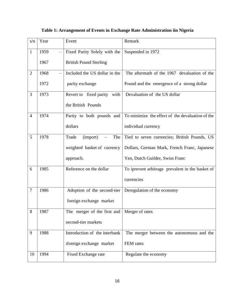
Table 1: Arrangement of Events iniExchange Rate Administration iin Nigeria

s/n Year Event Remark

1 1959 –

1967

Fixed Parity Solely with the

British Pound Sterling

Suspended in 1972

2 1968 –

1972

Included the US dollar in the

iparity exchange

iThe aftermath of the 1967 idevaluation of the

Pound and the iemergence of a istrong dollar

3 1973 Revertito fixediparity with

the British iPounds

iDevaluation of ithe US dollar

4 1974 Parity to both pounds and

dollars

To minimize ithe effect of ithe devaluation of the

individual currency

5 1978 Trade (import) – The

weighted ibasket of icurrency

approach.

Tied to seven currencies; British Pounds, US

Dollars, German Mark, French Franc, Japanese

Yen, Dutch Guilder, Swiss Franc

6 1985 Reference on the dollar To iprevent arbitrage iprevalent in the basket of

currencies

7 1986 iAdoption of the second-tier

iforeign exchange imarket

Deregulation of the economy

8 1987 The imerger of the first and

second-tier markets

Merger of rates

9 1988 Introduction of ithe interbank

iforeign exchange imarket

iThe merger between the autonomous and the

FEM rates

10 1994 iFixed Exchange rate iRegulate the economy

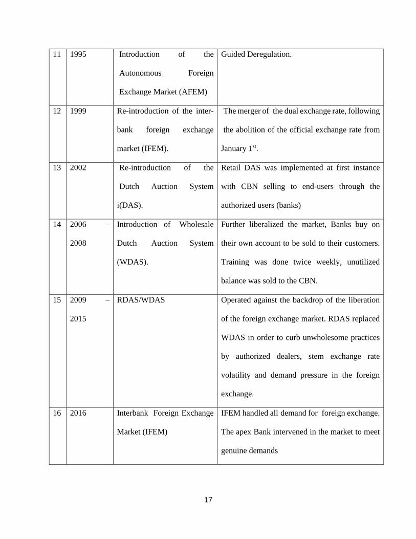
17

11 1995 iIntroduction of the

iAutonomous Foreign

iExchange Market (AFEM)

Guided Deregulation.

12 1999 Re-introduction of the inter-

bank foreign exchange

market (IFEM).

iThe merger of ithe dual exchange rate, following

ithe abolition of the official exchange rate from

January 1st.

13 2002 iRe-introduction of the

iDutch Auction System

i(DAS).

Retail DAS was implemented at first instance

with CBN selling to end-users through the

authorized users (banks)

14 2006 –

2008

Introduction of iWholesale

Dutch iAuction System

(WDAS).

Further liberalized the market, Banks buy on

their own account to be sold to their customers.

Training was done twice weekly, unutilized

balance was sold to the CBN.

15 2009 –

2015

RDAS/WDAS Operated against the backdrop of the liberation

of the foreign exchange market. RDAS replaced

WDAS in order to curb unwholesome practices

by authorized dealers, stem exchange rate

volatility and demand pressure in the foreign

exchange.

16 2016 Interbank iForeign Exchange

Market (IFEM)i

IFEM handled allidemand for iforeign exchange.

The apex Bank intervened in the market to meet

genuine demands

18

17 2016 –

2018

Flexible Exchange Rate

Interbank Market

Operates as a single market istructure through

ithe inter-bank/autonomous iwindow. The

Exchange Rate is market driven, FX Primary

dealers (FXPD) introduced.

Source: Central iBank of Nigeria (2007, 2009, 2016); CBN Press Releases, various Years”

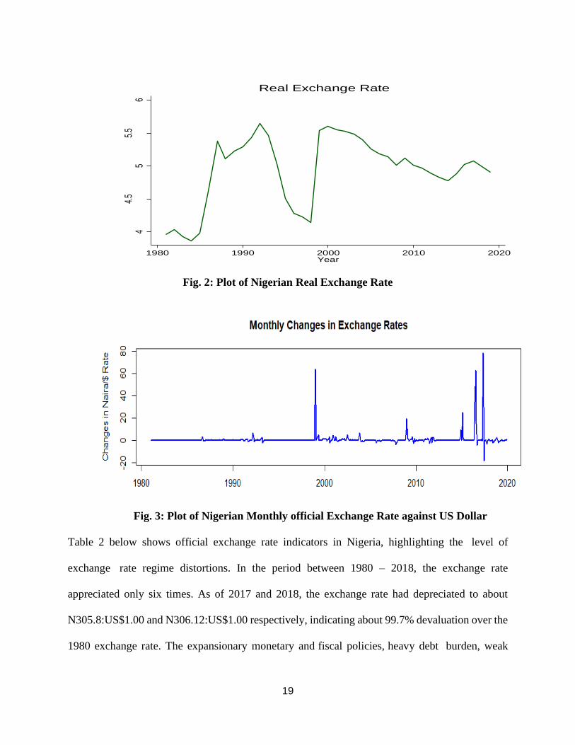
The currency rate of the Naira against the US Dollar has fallen by more than 800 percent since

Nigeria's independence, as shown in Figure 1. This means the Nigerian Naira is continuously

ilosing its value againsti Dollar. iThis situation iis almost true for the nature of Nigeria Naira

against iworldwide used iforeign currencies such as Euro, Pounds, Swiss, Franc, among others.

Fig. 1: Plot of Nigerian Nominal Exchange Rate

Figure 2 depicts the evolution of the Nigerian naira's real ibilateral exchange irate against the iUS

dollar from 1981 to 2019. Figure 3 reflects the month-to-month fluctuations in the Naira/Dollar

exchange irate showing ifrequent andi abrupt changes. We can observe frequent, sudden, and

haphazard ifluctuations in ithe exchange irate, with more ifluctuations in democratic iregimes than

military regimes, as democratic regime begins from 2009 till today.

02

46

lnnx

r

1980 1990 2000 2010 2020Year

Nominal Exchange Rate

19

Fig. 2: Plot of Nigerian Real Exchange Rate

Fig. 3: Plot of Nigerian Monthly official Exchange Rate against US Dollar

Table 2 below shows official exchange rate indicators in Nigeria, highlighting the ilevel of

exchange irate regime distortions. In the period between 1980 – 2018, the exchange rate

appreciated only six times. As of 2017 and 2018, the exchange rate had depreciated to about

N305.8:US$1.00 and N306.12:US$1.00 respectively, indicating about 99.7% devaluation over the

1980 exchange rate. The expansionary monetary andifiscal policies,iheavy debt iburden, weak

44.

55

5.5

6

lnrx

r

1980 1990 2000 2010 2020Year

Real Exchange Rate

20

iproduction base, over-reliance on the iimperfect foreign exchange imarket, input dependent

iproduction structure, ifragile export ibase, and weak non-oil export earnings, ifluctuations

inicrude oil revenues, an unguided itrade liberalization ipolicy,ispeculative activities, and

aggressive tactics (round-tripping) by authorized dealers, among other things, are all factors that

have been considered contributed to the misalignment of theireal exchange irate in Nigeria (Onoja,

2015)

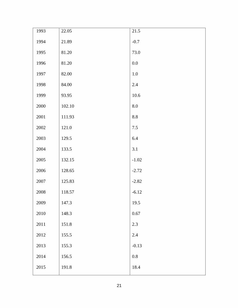
Table 2: Exchange Rate Movement in the Foreign Exchange Market.

Official Foreign Exchange Market

Year “(1) Rate (N:$) (2) Depreciation/Appreciation (%)

i1980

i1981

i1982

i1983

i1984

i1985

i1986

1987

1988

1989

1990

1991

i1992

0.55

0.62

0.67

0.72

0.76

0.89

2.02

4.02

4.54

7.39

8.04

9.91

17.30

-

11.2

7.5

6.94

5.26

14.6

55.9

49.8

11.5

38.6

9.3

19.9

42.7

21

i1993

i1994

i1995

i1996

i1997

i1998

i1999

i2000

i2001

i2002

i2003

i2004

i2005

i2006

i2007

i2008

i2009

i2010

i2011

i2012

i2013

i2014

i2015

22.05

21.89

81.20

81.20

82.00

84.00

93.95

102.10

111.93

121.0

129.5

133.5

132.15

128.65

125.83

118.57

147.3

148.3

151.8

155.5

155.3

156.5

191.8

21.5

-0.7

73.0

0.0

1.0

2.4

10.6

8.0

8.8

7.5

6.4

3.1

-1.02

-2.72

-2.82

-6.12

19.5

0.67

2.3

2.4

-0.13

0.8

18.4

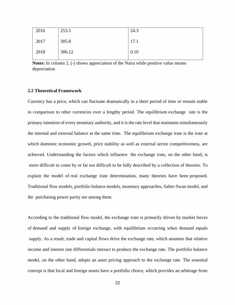
22

i2016

i2017

i2018

253.5

305.8

306.12

24.3

17.1

0.10

Notes: In column 2, (-) shows appreciation of the Naira while positive value means

depreciation

2.2 Theoretical Framework

Currency has a price, which can fluctuate dramatically in a short period of time or remain stable

in comparison to other currencies over a lengthy period. The equilibriumiexchange irate is the

primary intention of every monetary authority, and it is the rate level that maintains simultaneously

the internal and external balance atithe same time. iThe equilibrium exchange irate is the irate at

which domestic economic growth, price stability asiwell as external sector competitiveness, are

achieved. Understanding the factors which influence ithe exchange irate, on the other hand, is

imore difficult toicome by or far too difficult to beifully described by a collection of theories. To

explain the model ofireal exchange irate determination, many theories have beeniproposed.

Traditional flow models, portfolio balance models, monetary approaches, Salter-Swan model, and

the purchasing power parity are among them.

According to theitraditional flowimodel, the exchange irate is primarily driveniby marketiforces

ofidemand and supply ofiforeign exchange, with equilibrium occurring when demand equals

isupply. As a result, trade and capital flows drive the exchange rate, which assumes that relative

income and interest rate differentials interact to produce the exchange rate. The portfolio balance

model, on the other hand, adopts an asset pricing approach to the exchange rate. The essential

concept is that local and foreign assets have a portfolio choice, which provides an arbitrage from

23

expected returns and defines the exchange rate equilibrium. The monetary approach is based on

the idea that fluctuations in foreign exchange rates can be associated to changes in the demand and

supply of money in two countries. Variation in the exchange rate is attributed to factors such as

income and expected rates of return, as well as other factors that influence the supply and demand

for national currencies. The interest rate differentials, relative money supplies, and relative income

are the three primary drivers of the exchange rate, according to the monetary model since income

determines supply and demand for monies.

Cassel (1918) proposed the buying power parity hypothesis, which remains a useful way of

thinking about exchange rates today. According to this hypothesis, the exchange rates of two

countries will be equal to their respective national price levels. TheiPPP isifounded on LOOP, or

the law of oneiprice, whichistates that identical or similar items should cost the same in all nations

if transportation expenses, tradeibarriers, and quota constraints are abolished (Hakkio, 1992).

This theory asserts thatithe exchange rate between the currencies of any two countries should be

the same as theiratio of the two countries' general price levels, implying ithat exchange rates adapt

to compensate for pricing differences between countries.

The most basic and often used extension isibased on the concept of irelative purchasing ipower

parity (PPP), which holds thatithe equilibrium exchange irate is proportionate to the irelative

purchasingipower of the national currencies involved (Agherli et al. 1991). TheiPurchasing Power

iParity (PPP) hypothesisihas dominated policy debates,imodels, and empirical research for

decades. Changes in the inominal exchange rate are entirely offset (at least after a period) by

24

ichanges in ithe ratio of iforeign to domestic iprice levels, according to the hypothesis (Ajao and

Igbekoyi, 2012).

The final and theoretically more appealing approach is the Salter-Swan model, which attempts to

situate the equilibrium rate within real economic fundamentals. The strength of movements in ithe

equilibrium ireal exchange rate's ultimate determinants (also known as real exchange rate

fundamentals) affects the exchange rate. This approach is closely related to the iFundamental

Equilibrium iExchange Rate introduced by Ricci, iFerretti, and Lee (2008). The iFEER iis defined

as ithe real exchange irate that achievesiinternal and externalibalances at the same time. It iis one

of ithe most widely used ideas in calculating equilibrium ireal exchange rates. Fundamentals can

partially explain real exchange rate behavior over imedium to ilong time ihorizons, according to

experts.

Changes in ithe equilibrium ireal exchange irate are thought to represent, in certain situations,

equilibrium conditions brought about by fundamental changes (Edward, 1992). Real exchange rate

volatility is caused by a variety of reasons. Openness of an ieconomy, production, inflation, interest

rates, local and foreign imoney supply, iexchange rate iregime, and monetary authority

independence are some of ithese characteristics (Stancik, 2007). Each of these factors has varying

degrees of influence, depending on the economic situation of a given country. As a result, countries

in transition (such as Nigeria) are more exposed to these factors, which might have an impact on

monetary policy decisions. In his examination of developing Asia countries, Juthathip (2009)

found that the actual exchange rate is governed by five main fundamental determinants.

iProductivity differences, openness, iterms ofitrade, netiforeign assets, andigovernment ispending

are among them. It is possible to argue that ireal exchange irates in quickly changing countries

25

will be influenced by these ireal shocks. The extent to iwhich differentishocks affect ireal exchange

irate behavior, on the other hand, iis determinediby country-specific characteristics. The itypical

method ito real exchange irate equilibrium modeling is to express the theoretical relationship

ibetween the real exchange rate and theimost essential "fundamentals," or real variables, that

determine its fluctuations.

iBased on the extant iliteratures, the partial analyses of the major ifundamentals considered in this

thesis, especially in relation with theireal exchange rate are discussed asifollow.

The Real exchange Rate

The ireal exchange irate (rxr) is defined as the ibilateral nominal exchange irate that is the adjusted

by the ratio of ithe foreign iprice level (pf) to the domestic price index (P). It is expressed

mathematically as,

rxr = e P

Pf

In line with this definition, a rise inithe real exchange irate index indicates aireal depreciation,

while aifall indicates aireal appreciation. It is a dependent variable in this study.

iThe NominaliExchange Rate

The iprice of one icurrency in iterms of another country's currency is known as the inominal

exchange irate. The inominal exchangei rate growth rate is projected toihave aipositive partial sign

on the real exchange rate. As a result, an increase or reduction in the inominal exchange irate

causes a rise or fall in the real exchange rate. The capacity of inominal exchange rate ifluctuations

to effect theireal exchange irate will be determined by how well macroeconomic policies are

26

aligned with the nominal exchange rate's goal. One strategy for accelerating real exchange rate

adjustment could be to modify theinominal exchange irate.

The Money Supply

The partial effect of domestic imoney supply on ithe real exchange irate is projected to be negative.

All exchange rate itheories agree that increasing the local money supply will lead the domestic

currency to devalue; the only difference is the transmission mechanism. Money supply has a

negative irelationship with the iexchange rate, and a rise in the imoney supply icauses the domestic

icurrency to depreciate. The normal exchange rate and the effective exchange rate both rise when

monetary policy is tight. The econometric evidence of the imoney supply effect on ithe exchange

irate, on ithe other ihand, is diverse and inconclusive. The impact of monetary policy on ithe real

iexchange rate is determined iby whether it is expansionary or contractionary. A rise in the money

supply, which represents an expansionary imonetary policy, puts upward pressure on domestic

prices, causing the ireal exchange irate to appreciate. If inflation does not adjust immediately under

a floating rate system, the increase in money depreciates the exchange rate. Under the fixed

exchange rate regime, however, an increase in money will result in a devaluation of the currency.

The Rate of inflation

Because differing trends in national inflation rates commonly produce payments imbalances,

several studies have concluded that inflation rate movement is at ileast as iimportant as any other

factor in affecting ireal exchange irate volatility. Because ithe real exchange irate is determined

using the inominal exchange irate and the iprice level, itiis desirable to include the direct effect of

inflation. Excess domestic credit raises theiprice level, resulting in aireal exchange irate

27

appreciation. As a result, inflationiis linked toithe exchange irate of the home currency against

theiforeign currency.

Real Growth of Domestic Product (Real GDP)

It is generally expected that the lower the level of economic development, the less developed and

inefficient would be both the goods market and the factor markets. Import demand elasticities are

low because domestic replacements for imported commodities are not available. Furthermore,

there is little opportunity for changing trade products supply between domestic and international

markets. There thus would appear to be reasons why the equilibrium ireal exchange irate would

vary negatively wiheithe degree of economic development.

Trade Openness

The openness of ithe economy is usedi as a iproxy for the trade policy and its partial expected

effect on the ireal exchange irate is negative. The general view is that trade liberalization

characterized by reductions in tariffs and/or the elimination of quantitative restrictions will lead to

increased trade. A rise in OPN (i.e., more open) therefore results in a real exchange rate

depreciation. If the economy is more opened and protection is reduced, the demand for domestic

goods and their prices will fall, thus resulting to exchange rate depreciation. An elimination of

import duties allows importers to buy more foreign exchange for the same level of total

expenditures. The resulting increased foreign exchange demand under a free-floating exchange

rate iregime leads to a idepreciation of ithe real exchange irate. Under ifixed exchange irate

regimes, the conversion of more foreign currency into domestic currency leads to the expansion

28

of imoney supply, a rise in domestic iinflation and an appreciation of ithe real exchange irate

(Obadan, 1994).

Government Expenditure

In establishing the behavior of the equilibrium ireal exchange irate, the expected sign ofithis

variable could be ipositive or negative. iIncreased government spending boosts domestic demand

for both tradables and nontradables, with excess idemand for nontradables pushing up costs and

causingireal exchange irate appreciation. The ireal exchange irate, on the other hand, will

depreciate if a bigger share of government spending is spent on the itradable sector irather than

nontradables consumption.

2.3 Empirical Literature

Many factors influence ireal exchange irate volatility, and the attempt to understand these factors

has resulted in a great number of empirical studies ithat have already proven to be useful in ithe

literature. Many factors, including output, inflation, interest rate, money supply, an economy's

openness, and the exchange rate regime, are listed as causing variations in ithe real exchange irate.

Nonetheless, the extent ito which each of these elements has an impact varies and is dependent on

ithe economic situation of a certain country.

Edwards (1989) pioneered the fundamentals models of real exchange rate setting for

underdeveloped countries. He discovered that only real variables affect the ilong-run equilibrium

real exchange rate while building a model of real exchange irate determination for calculating

29

equilibrium value for a ipanel of 12 developing nations. Real and nominal factors, on ithe other

hand, explained ireal exchange rate variations.

Excess idomestic credit creation, openness, and technological progress significantly contribute to

ireal exchange irate appreciation, according to Siddiqui et al. (1996), while estimating the

determinants of ireal exchange irate for Pakistan. They also find that increases iin governmental

expenditures lead to depreciation iin real exchange irate. Also, both monetary and real sector

variables significantly influence the stability route idetermination of the ireal exchange irate.

Chowdhury (1999) uses OLS to investigate ithe extent to which ireal and inominal factors may

explain the evolution of the ireal exchange irate in Papua iNew Guinea from 1970 to 1994. The

findings reveal ithat nominal devaluation has a significant iimpact on ireal exchange irate behavior.

The ireal exchange irate of Papua iNew Guinea appreciates due to net capital flow, foreign aid,

expansionary imacroeconomic ipolicies, and trade irestrictions. That, 1% iincrease in capital flow,

trade restriction, excess imoney supply over GDP growth icauses the real GDP to appreciate iby

0.35%, 0.08%, and 0.05%, respectively.

Mungule (2004) used the cointegration itechnique to investigate ithe determinants of ithe real

exchange irate in Zambia. He identified a long-run equilibrium relationship between ithe real

exchange irate and the iterms of trade, icapital inflow, the economy's proximity, and surplus

isupply of domestic icredit (i.e., the fundamental determinants).

The real exchange irate is governed by five major ifundamental variables ithat represent medium

to long-run fundamentals, according to Juthathip (2009)'s findings ifor developing Asia.

30

Differential productivity, openness, terms of itrade, net iforeign assets, and government spending

are all factors considered.

Oriavwote (2012) empirically tests the impact of changes in virtual determinants of ithe real

exchange irate in Nigeria using dataifrom 1970 to 2010. The nominal effective exchange irate,

capital flow, Nigeria's openness to international commerce, and real GDP are all major factors of

Nigeria'sireal effective exchange irate, according to the research. The ECMifindings suggestithat

rising prices, capital flow, capital accumulation, and trade openness all strengthen Nigeria'sireal

effective exchange irate.

From 1981 to 2008, Ajao and Igbekoyi (2013) investigate the drivers of ireal exchange irate

volatility in iNigeria. An error correctionimodel was used to evaluate ithe various ideterminants of

ithe real exchange irate in Nigeria after the volatility was determined using ithe GARCH (1, 1)

technique. GARCH parameters suggest ithat real exchange irate volatility shocks in Nigeria are

quite persistent. For the iperiod under iconsideration, government spending, trade openness, real

exchange irate, and ireal interest rate are all important factors of ireal exchange irate volatility.

This thesis builds on previous research by econometrically assessing the macroeconomic

determinants of ithe real exchange irate in iNigeria from 1981 to 2019.

3. Data Description

3.1 Data Sources

The analysis is based on thirty-nine years of data coveringithe period from 1981 until 2019 to

examine theibehavior ofithe real exchange irate and the relationship with its macro-economic

determinants. The time series in annual frequency were obtained from various publications of the

31

World Bank (WBI), the Nigerian Central Bank (CBN), and the Organization of Petroleum

Exporting Countries (OPEC).

3.2 Definitions and Sources of Variables

Previous research has found that macroeconomic variables may determine the long irun

equilibrium ivalue of the ireal exchange rate. Based on the prior findings in the literature, the

following variables are likely to play a key role in explaining the real exchange rate. These are

precisely defined, proxied, and constructed in the Table 3 below.

Table 3: Definition and Sources of Variables

Variable Notation Construction Source

iNominal Exchange

Rate

NXR Bilateral iExchange rate of iNigeria Naira

against ithe US Dollar

Central iBank

of Nigeria

Real iExchange Rate RXR Nominal Exchange Rate/ratio of

Consumer iPrice Index

CBN

Money iSupply MS Broad Money World Bank

Inflation Rate INF Domestic Rate of Inflation World Bank

Total Output RGDP Real Gross iDomestic Product World Bank

iTrade Openness OPN Import + Export / Real GDP World Bank

Oil Price OILP Global Oil Price OPEC

Foreign Reserves FXR Total External Reserves Stock of Nigeria World Bank

External Debt EXD Total stock of external debt World Bank

Government

iExpenditure

GEXP Government Total Expenditure (recurrent

andi capital)

World Bank

Source: Researcher’s Compilation

32

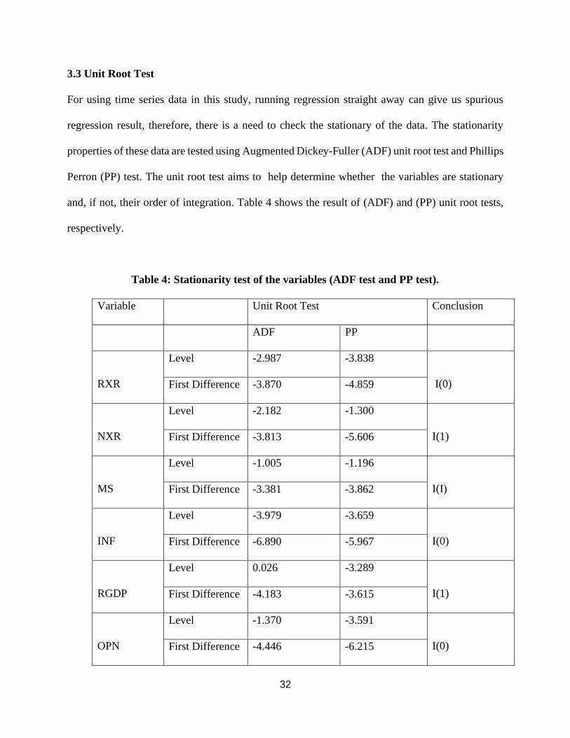
3.3 Unit Root Test

For using time series data in this study, running regression straight away can give us spurious

regression result, therefore, there is a need to check the stationary of the data. The stationarity

properties of these data are tested using Augmented Dickey-Fuller (ADF) unit root test and Phillips

Perron (PP) test. The unit root test aims to ihelp determine whether ithe variables are stationary

and, if not, their order of integration. Table 4 shows the result of (ADF) and (PP) unit root tests,

respectively.

Table 4: Stationarity test of the variables (ADF test and PP test).

Variable Unit Root Test Conclusion

ADF PP

RXR

Level -2.987 -3.838

I(0) First Difference -3.870 -4.859

NXR

Level -2.182 -1.300


MS

Level -1.005 -1.196

I(I) First Difference -3.381 -3.862

INF

Level -3.979 -3.659


RGDP

Level 0.026 -3.289


OPN

Level -1.370 -3.591


33

OILP

Level -1.027 -2.315

I(I) First Difference -4.706 -5.915

FXR

Level -1.097 -3.245


EXD

Level -2.262 -2.359


GEXP

Level -0.344 -2.039


iCritical

Value

1% -3.594 -4.159

5% -2.936 -3.504

10% -2.602 -3.182

Source: Researcher’s Compilation

Both methods generally agree and show that several of the variables are not stationary except real

exchange rate, inflation rate (INF), and trade openness (OPN) variables that are stationary in levels.

All other variables are stationary after taking the first difference. At the ifirst differencing, ithe

calculated iADF and iPP test statistics reject the unit root's null hypothesis when icompared with

their icorresponding critical ivalues at 5%. Hence, the ADF and PP tests show ithat all variables

are iintegrated of order 0 or order 1, i.e., I(0) or I(I). This implies that I can apply the ARDL

methodology for the model.

34

4. Methodology

4.1 Model Specification

The ireal exchange irate is represented as a ifunction of the inominal exchange rate, money supply,

inflation rate, real iGDP growth, foreign reserves, itrade openness, the global oil price, and the

stock of external idebt as follows, ibased on the theoretical background and data availability:

RXR = f (NXR, MS, INF, RGDP, OPN, OILP, FXR, EXD GEXP) …………. (1a)

Where,

RXR = Real Exchange Rate

NXR = Nominal Exchange Rate

MS = Money supply

INF = Inflation Rate

RGDP = Real GDP growth

OPN = Trade Openness,

OILP = Global Oil Price

FXR = Foreign Exchange Reserves

EXD = External Debt Stock

GEXP = Government Expenditure

For empirical estimation, the general functional form in equation (1a) is specified in the following

log linear regression:

lnRXRt = α0 + α1lnNXRt + α2lnMSt + α3lnINFt + α4lnRGDPt + α5lnOPNt + α6lnOILPt

+ α7lnFXRt + α8lnEXDt + α8lnGEXPt + εt

Where, α0 = Constant term εt = error/stochastic term, αi, i = (1, 2, …,9), the parameters to be

estimated.

35

It is possible that ithe relationship ibetween the ireal exchange irate on the left and its

macroeconomic factors on the right is not strictly contemporaneous. As a result, as shown in the

Autoregressive iDistributed Lag (ARDL) model below, the regression accounts for time lags in

the link between ithe real exchange irate and its macroeconomic drivers.

lnRXRt = α0 + Σα1ilnNXRt-i + Σα2ilnMSt-i + Σα3ilnINFt-i + Σα4ilnRGDPt-i + Σα5ilnOPNt-i

+ Σα6ilnOILPt-i + Σα7ilnFXRt-i + Σα8ilnEXDt-i + Σα9ilnGEXPt-i + εt .... (2)

The model's optimal lag length would be determined using the Schwarz Bayesian Information

Criteria (SBIC).

4.2 Cointegration Analysis

The Autoregressive distributive ilag (ARDL) approach ito cointegration is being used to establish

the ilong run itrelationship between ithe real exchange irate and its macroeconomic determinants.

This approach is preferred because it can ibe applied ifor series of different orders of integration,

it also allows iflexibility to incorporate ithe required inumber of lags ineeded to describe the

behaviour of the variable of interest, as well it also good for a lower sample size.

The cointegration ibetween the ireal exchange irate and the mentioned variables is investigated

using the ARDL bounds testing approach established by Pesaran et al (2001). For empirical

inquiry, this method simultaneously provides long and short run estimations. The error correction

representation of the ARDL model below (i.e., equation(4)) is required for the correct definition

36

of such a relationship that will reflect the short run variations that may have occurred in estimating

the long run cointegrating equation.

ΔlnRXRt = α0 + Σα1iΔlnNXRt-i + Σα2iΔlnMSt-i + Σα3iΔlnINFt-i + Σα4iΔlnRGDPt-i

+ Σα5iΔlnOPNt-i +Σα6iΔlnOILPt-i + Σα7iΔlnFXRt-i + Σα8iΔlnEXDt-i

+ Σα9iΔlnGEXPt-i + 𝛅1ilnRXRt-1 +𝛅2ilnNXRt-i + 𝛅3ilnMSt-i + 𝛅4ilnINFt-i

+ 𝛅5ilnRGDPt-i + 𝛅6ilnOPNt-i + 𝛅7ilnOILPt-i +𝛅8ilnFXRt-i + 𝛅9ilnEXDt-i

+ 𝛅10ilnGEXPt-i + εt …(4)

Where the parameters 𝛅 = (𝛅1, 𝛅2, 𝛅3, … ,𝛅10), are the long-run coefficients, and the parameters α =

(α1, α2, α3, …, α9), are to capture any short-run relationship in the main ARDL model.

ARDL ibounds testing method to cointegration is applied by comparing the value of F-test of

ilagged level variables ithrough variable addition itest with ithe critical bound presented by Pesaran

et al., (1996, 2001). The lower bound is ithe critical value ifor I(0) variables as well as ithe upper

ibound is for I(I) variables. If the computed value of the F-statistics above the upper ibound critical

value, there is evidence ifor the existence of ilong run connection between ithe variables. If the

value is lesser than the ilower critical bound, there is evidence of ino long run connection. If the

value of iF-statistic is in the middle of the upper ibound and lower ibound, then it iis inconclusive.

Once the existence of cointegration is proven, the estimation of long run ARDL model and an error

correction model (ECM) that covers short-run dynamics was carried out. This model is stipulated

as follows:

37

ΔlnRXRt = α0 + Σα1iΔlnNXRt-i + Σα2iΔlnMSt-i + Σα3iΔlnINFt-i + Σα4iΔlnRGDPt-i

+ α5iΔlnOPNt-i + Σα6iΔlnOILPt-i + Σα7iΔlnFXRt-i + Σα8iΔlnEXDt-i

+ Σα9iΔlnGEXPt-i + 𝛅ECM(-1) + εt …….(5)

The long-run relationshipibetween the right-hand side variables and the left-hand side variable is

captured by ECM (-1), and while εt isithe error term, the ECM (-1) iis the error icorrection term.

The short run impacts are assessed using the coefficients of ithe differenced terms (αi) whereas

ithe coefficient of ithe error correction iterm (𝛅) variable contains iinformation on whether ipast

values of variables have an impact on current values. The ECM coefficient's sign, magnitude, and

significance indicate how possible each variable is to return to equilibrium.

5. Empirical Results

5.1 Cointegration Test

The existence of cointegration is examined using the ARDL bounds testing approach. While this

approach does not restrict all variables to be of the equal order of integration, it also allows

flexibility in the required number of lags. It is arguably suitable when the sample size is small.

The computed F-statistic of the bounds test is stated in Table 5 below. The iresults reveal ithat the

calculated F-statistic of 12.171 which is more than the upper bound of the critical values at 5%

and 10%, as Pesaran et al. (1997) calculated. This is evidence ifor the ipresence of a cointegration

connection, which implies ithe rejection of the inull hypothesis of no cointegration.

38

Table 5: Result of Bounds Test for Cointegration

5% Critical Value 10% Critical Value

K I(0) I(I) I(0) I(I)

9 2.14 3.30 1.88 2.99

Computed F-statistic – F(LNREE│LNNEER, LNMS, LNINF, … , LNGEXP) = 12.171

I proceed to estimate equation (4) for the long-run elasticities because the computed F-statistics

are above the critical value, indicating the existence of a long-run relationship. Table 6 shows the

results of the selected optimal lag length for the ARDL model (1 1 2 1 0 1 2 0 1 1) using Schwarz

Bayesian Information Criteria (SBIC) with a maximum lag of 2.

The computed long-run coefficients reveal that ithe real exchange irate and its determinants have

ailong-run relationship. iThe real exchange irate is influenced by the inominal exchange irate,

imoney supply, inflation irate, real GDP, foreign currency reserves, and the stock of external debts

in the ilong run. At 1% and 5% levels, the coefficients of global oil price, government expenditure,

and economic openness are not statistically different from zero. In the ilong run, the inominal

exchange rate, real GDP and, inflation rate are positively and significantly associated to the ireal

exchange rate. iThis means that a i1% increase in these variables is related with an iincrease of

1.287%, 1.219%, and 2.309%, respectively, in the ireal exchange rate.

The foreign reserves, money supply, and external debt are inegatively and significantly related to

the ireal exchange rate. Implying that a 1% increase in each of these variables iis associated with

a decrease of 1.033%, 0.561%, and 0.776%, respectively, in the real exchange rate. This imeans

39

that in the case of Nigeria, increases in money supply, foreign exchange ireserves, and external

debt iresult in real exchange irate appreciation during the sample period. Within the selected period

of 1981-2019, the inominal exchange irate, inflation, and ireal GDP all contributed to a

idepreciation of the ireal exchange rate in Nigeria.

Table 6: Estimated Long Run Coefficients Using ARDL Approach

Regressor Coefficient Standard Error t-statistic Prob.

LnNXR 1.2874 .12354 10.42 0.000

LnMS -1.0327 .11426 -9.04 0.000

LnINF 1.2189 .38006 3.21 0.005

LnRGDP 2.3092 .59351 3.89 0.001

LnOPN -0.3209 .16304 -1.97 0.065

LnOILP -0.0039 .31207 -0.01 0.990

LnFXR -0.5613 .17644 -3.18 0.005

LnEXD -0.7261 .27261 -2.68 0.016

LnGEXP 0.2462 .13589 1.81 0.087

5.2 The Short-run Aspects of Real iExchange Rate in iNigeria

The ARDL model's error correction irepresentation captures the short-run analysis of ithe real

exchange irate. While the ECM is useful for estimating the irelationship between imacroeconomic

variables and ithe real exchange rate, the goal is to illustrate the speed with which the rate is

adjusting to its equilibrium state.

40

Table 7i shows the estimates of ithe error correction model's short-run coefficients, with an

evaluation of the results confirming that the overall fit of the model is satisfactory at R2 = 0.9208.

This means that the model's independent variables collectively accounted for 92.08 percent of the

overall variation in the ireal exchange rate, particularly the significant short- and ilong-run

relationship between ithe nominal and ireal exchange rates.

In the short irun, the inominal exchange rate, imoney supply, inflation, trade openness, oil price,

and foreign debt are all strongly linked to the ireal exchange rate. iIn the short irun, the lagged

values of money isupply and global oil price were also highly related to the ireal exchange rate.

The coefficient of ECM(-1), as could be observed in the table, is negative (-0.146) and highly

significant (0.006). This means that the model has a self-adjusting mechanism that aligns the

variable's short-run dynamics with its long-run values.

Table 7: Error Correction iModel Representation for ithe Selected ARDL iModel

Variable Coefficient Std. Error t-Statistic Prob.

C 1.41702 1.35054 1.05 0.308

ΔlnNXR 1.13633 0.04799 23.68 0.000

ΔlnMS -0.11777 0.04297 -2.74 0.000

ΔlnMS(-1) -0.13492 0.04966 -2.72 0.013

ΔlnINF 0.02240 0.00947 2.36 0.014

ΔlnOPN -0.07756 0.01679 -4.26 0.030

ΔlnOILP 0.08712 0.03383 2.57 0.000

ΔlnOILP(-1) -0.04748 0.02195 -2.16 0.019

ΔlnEXD -0.12349 0.03458 -3.57 0.044

ECM (-1) -0.14560 0.04669 -3.12 0.006

R2 = 0.9982 Akaike Info Criterion = -10.615

Adj R2 = 0.9964 Schwarz Criterion = -5.726

Log likelihood = 106.6061 F-statistic(18, 18) = 144.71

Durbin-Watson = 2.4852 Prob (F-statistic) = 0.0000

41

Most of the variables with statistically significant long-run coefficients also have statistically

significant short-run coefficients. In ithe short run, ithe real exchange irate is positively and

significantly related to the inominal exchange irate, inflation irate, and global oil price. A 1%

increase iin the oil price, nominal exchange irate, and inflation rate in the preceding year, is related

with increases in the ireal exchange irate of 1.136 percent, 0.022 percent, and 0.087 percent,

respectively, indicating a depreciation of ithe real exchange irate in the ishort run.

In the ishort run, a rise in the money isupply is related with a decrease in the ireal exchange rate,

both immediately and after one iyear. In the ishort run, an iincrease in external debt is related with

a decrease in the ireal exchange irate, as is observed in the long run. An iincrease in the lagged

value of oil price relates to a idecrease in ithe real exchange irate, also in ithe short run. iThe real

exchange irate appreciates the following year when the money supply and global oil price rise in

a particular year. It can be seen that in ithe long and short run, both monetary policy in iterms

of money isupply, and fiscal policy in terms of external debts can be exploited to effect the

equilibrium ireal exchange rate.

It is also worth noting that ithe nominal exchange irate and the ireal exchange irate in Nigeria are

linked. In both ithe long and short run, a idepreciation of ithe nominal exchange irate leads to a

depreciation of the ireal exchange rate. Nigeria's real exchange fluctuation would be stabilized by

effective control and management measures to stable the nominal exchange rate.

42

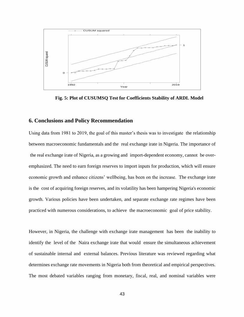
5.3. Diagnostic tests

There is no evidence of serial correlation or heteroscedasticity in the model, according to the

diagnostic test results (Table 8), and normality is not rejected. Since (P-value = 0.4226 > 0.05),

the variance of the residuals is constant, as per the heteroscedasticity test. The Jarque-Bera test of

normality shows that the model's residuals are normally distributed (P-value = 0.478 > 0.05). As

displayed in Figures 4 and 5, the cumulative sum of recursive residuals (CUSUM) and the

cumulative sum of squares of recursive residuals (CUSUMSQ) are within the critical boundaries

for the 5%, suggesting ithat the model's coefficients are constant across the sample period. As a

result, the model is clearly not mis-specified.

Table 8: Diagnostic tests for underlying ARDL ( 1 1 2 1 0 1 2 0 1 1) model

Fig. 4: Plot of CUSUM Test for Coefficients Stability of ARDL Model

Chi2 Statistic’s value p Value

Breusch-Godfrey LM test Serial correlation

Jarque-Bera test Normality

Breusch-Pagan-Godfrey: Heteroscedasticity

2,944

0.50

37.00

0.0862

0.478

0.4226

CUSU

M

Year

CUSUM lower upper

1981 2019

0 0

43

Fig. 5: Plot of CUSUMSQ Test for Coefficients Stability of ARDL Model

6. Conclusions and Policy Recommendation

Using data from 1981 to 2019, the goal of this master’s thesis was to investigate ithe relationship

between macroeconomic fundamentals and the ireal exchange irate in Nigeria. The importance of

ithe real exchange irate of Nigeria, as a growing and iimport-dependent economy, cannot ibe over-

emphasized. The need to earn foreign reserves to import inputs for production, which will ensure

economic growth and enhance citizens’ wellbeing, has been on the increase. iThe exchange irate

is the icost of acquiring foreign reserves, and its volatility has been hampering Nigeria's economic

growth. Various policies have been undertaken, and separate exchange rate regimes have been

practiced with numerous considerations, to achieve ithe macroeconomic igoal of price stability.

However, in Nigeria, the challenge with exchange irate management ihas been ithe inability to

identify the ilevel of the iNaira exchange irate that would iensure the simultaneous achievement

of sustainable internal andi external balances. Previous literature was reviewed regarding what

determines exchange rate movements in Nigeria both from theoretical and empirical perspectives.

The most debated variables ranging from monetary, fiscal, real, and nominal variables were

CUSU

M sq

uare

d

Year

CUSUM squared

1992 2019

0

1

44

selected and analyzed to achieve the purpose of this investigation. The nominal exchange rate,

foreign reserves, money supply, inflation rate, real GDP, trade openness, external debt,

government expenditure, and global oil price are all variables in my model. The data on these

variables were subjected to the Augmented Dickey-Fuller (ADF) and Philips Perron (PP) tests to

look for unit roots. Apart from the ireal exchange irate, inflation, and openness, which are

stationary in levels, both techniques indicate that many variables are simply stationary in

differences.

The Autoregressive Distributed Lag (ARDL) bounds testing approach was used to assess the long-

run connection between the variables. iThe real exchange irate and the stated macroeconomic

fundamentals have a long-run irelationship, as per my findings. In the long run, ithe real exchange

rate iis influenced by the money supply, inflation rate, real GDP, foreign exchange reserves,

nominal exchange irate, and stock of external debts. During the period 1981-2019, the coefficients

of global oil price, government expenditure, and economic openness are not statistically

significant. The short-run aspects were examined using the ARDL's error correction

representation, and the results show that ithe nominal exchange irate, inflation rate, and global oil

price are all positively and significantly related to the ireal exchange rate. The increase in external

debt, money supply, and global oil price, instead, leads to ireal exchange irate appreciation.

As a result, it is suggested that the government should try and control these variables that have a

direct effect on real exchange rate variations. A limit on how much the exchange rate can fluctuate

should also be established. Since inflation has been identified as one of the causes linked to real

exchange rate depreciation, measures aimed at stabilizing the inflation rate should be implemented.

45

iThere is also a ineed for a review of the trade liberalization, which permitted all kinds of goods to

be imported into the country, resulting in heavy pressure on iforeign exchange ireserves and ithe

exchange rate. The sourcing, disbursement, and pricing of foreign exchange should be considered

as a significant part of the country's major policy objectives, with a particular focus on diversifying

the sources of foreign exchange inflow, particularly enhancing the supply of foreign exchange

from the non-oil sector, and effective demand management.

The productive sector should continue to receive priority in foreign exchange disbursement with

appropriate control measures to avoid round-tripping practice to the parallel market. Since the

investment inflow will generate more foreign reserves for the country, there is a need to encourage

an enabling environment that promotes investment into the country. The sectors such as

agricultural, mining, and industrial sectors should be reformed toward encouraging exports and

increasing investment inflows.

It is also suggested that efforts be made to enhance the consumption of goods produced in Nigeria,

including the use of locally sourced raw materials by Nigerian enterprises in order to boost foreign

exchange revenues. This implies that local industries should be encouraged to source their raw

materials locally (Oladapo, F. & Oloyede, J.A, 2014).

46

7. References

Adewuyi, A.O (2005). Trade and exchange rate policy reform and export performance of the real

sector: the case of Nigeria. Selected papers for the 2005 Annual Conference of the Nigeria

Economic Society.

Ahmet, N.K & Mehtap, K (1997). The real Exchange rate Definitions and calculation.

Central Bank of the iRepublic of Turkey: Research Department. No: 97/1

Ajao, M.G & Igbekoyi, O.E (2013). The iDeterminants of Real iExchange Rate Volatility in

Nigeria: Academic Journal of Interdisciplinary Studies. Vol 2, No. 1

Aliyu, S.U.R, (2008). Exchange iRate Volatility and Export iTrade in Nigeria: An Empirical

investigation. An MPRA paper No. 13490

Balassa, B. (1964). The iPurchasing Power iParity Doctrine: A reappraisal. Journal of iPolitical

Economy, 72, 584-96. http://dx.doi.org/10.1086/258965

Boniface, A. (2012). iDeterminants of Real Exchange Rate in iPapua New Guinea. Working iPaper

BPNGWP2012/04. Bank of Papua iNew Guinea Port Moresby iPapua New Guinea

Central bank of Nigeria (2019). The iforeign exchange imarket and its management in Nigeria:

CBN Briefs, 2001 edition.

Chowdhury, M.B. (1999). The iDeterminants of iReal exchange rate iin Papua New iGuinea. Asia

iPacific Press ISSN 1441-9858, ISBN 0 7315 3618 5.

Edwards, S. (1994). Real and imonetary determinants of ireal exchange rate ibehaviour: theory

and evidence from developing countries. Institute for iInternational Economics, Washington

Ewubare, D.B and Merenini, C.D (2019). The Effect of Exchange Rate Fluctuation on Foreign

Trade-in Nigeria. International Journal of Scientific Research and Engineering

Development-– Volume 2 Issue 1.

Ibrahim U.A & Muazu A. (2020): Effect of Bureau De Change Establishment on the Stability of

iExchange Rates in Nigeria. European Journal of Business and Management. Vol.12,No.6,

Juthathip, J. (2009). Equilibrium iReal Exchange rate iMisalignment and iExport Performance in

http://dx.doi.org/10.1086/258965

47

Developing Asia: ADB iEconomics, Working Paper No. 15.

Mungule, K.O. (2004) The ideterminants of Real iExchange Rate in Zambia. African Economic

iResearch Consortium, Paper 146 Nairobi.

Obadan, M.I (1994). Foreign Exchange management and Stability of the Nigerian Economy,

1976-2016 CBN Bullion Vol. 40 No. 1-40.

Obaseki, P.J (2001). Meeting the foreign exchange needs of the ireal sector of the iNigerian

economy. A paper presented at the CBN Second Monetary Policy forum on the Theme:

Exchange Rate Determination and Foreign Exchange management in Nigeria, February 7.

Oladapo, F & Oloyede, J.A (2014). Foreign Exchange Management and the Nigerian Economic

Growth (1960 – 2012): Published by European Centre for Research Training and

Development UK

Onoja, J. E. (2015). A Dynamic Analysis of the Impact of Capital Flight on Real Exchange rate in

Nigeria. IOSR Journal of Economic and Finance. Volume 6. Issue 1, PP 31-35

Onwughai, E.A. (2010). Covid-19 and the Nigerian Economy: Evidence from the Foreign

Exchange Rate.

Oriavwote, V.E & Oyovvwi, D.O (2012). The Determinants of Real Exchange Rate in Nigeria:

International Journal of Economics and Finance, Vol. 4, No. 8, 2012

Pesaran, H.M., Shin, Y. & Smith, R.J. (2001). Bound Testing Approach to the analysis of Long-

Run Relationships. Working Paper. University of Cambridge.

Ricci, L.A., Forretti, G.M, and Lee, J. (2008). Real exchange irate and Fundamentals: Across-

Country Perspective, IMF Working Paper.

Sharmila, T. & Bangi, S. (2010). Stock Price and Foreign Exchange Rate in Malaysian Context

Solomon, T.N. (2015). The Effect Of Foreign Exchange Rate Fluctuations On Export Earnings:

Evidence From Flower Industry In Kenya. A research project submitted to the university

of nairobi

48

Stancik, J. (2007). iDeterminants of iExchange Rate Volatility: The Case of the New EU

Members’. iCzech iJournal of iEconomics and iFinance 56(9&10)56-56-72.

Wamukhoma, W.O (2013). The iEffect of Foreign Exchange Rate iFluctuations on Horticultural

Export iEarnings in Kenya.

Wasiu, A.Y., et al., (2019). Determinants of iExchange Rate in iNigeria: A Comparison of the

Official and Parallel Market Rates: Research Gate,

https://www.researchgate.net/publication/337297446

Williamson, J. (1994). Estimates of FEERs in estimating equilibrium Exchange Rate by J.

Williamson (ed): Washington, Institute of International Economics.

An Econometric Analysis Of the Determinants of

Documents

Transcript of An Econometric Analysis Of the Determinants of