
An atom trap trace analysis (ATTA) system for … atom trap trace analysis (ATTA) system for...
142
An atom trap trace analysis (ATTA) system for measuring ultra-low contamination by krypton in xenon dark matter detectors Tae Hyun Yoon Submitted in partial fulfillment of the requirements for the degree of Doctor of Philosophy in the Graduate School of Arts and Sciences COLUMBIA UNIVERSITY 2013
Transcript of An atom trap trace analysis (ATTA) system for … atom trap trace analysis (ATTA) system for...
An atom trap trace analysis (ATTA) system formeasuring ultra-low contamination by krypton in
xenon dark matter detectors
Tae Hyun Yoon
Submitted in partial fulfillment of the
requirements for the degree
of Doctor of Philosophy
in the Graduate School of Arts and Sciences
COLUMBIA UNIVERSITY
2013

c©2013
Tae Hyun Yoon
All Rights Reserved

ABSTRACT
An atom trap trace analysis (ATTA) system formeasuring ultra-low contamination by krypton in
xenon dark matter detectors
Tae Hyun Yoon
The XENON dark matter experiment aims to detect hypothetical weakly interacting mas-
sive particles (WIMPs) scattering off nuclei within its liquid xenon (LXe) target. The trace
85Kr in the xenon target undergoes β-decay with a 687 keV end point and 10.8 year half-
life, which contributes background events and limits the sensitivity of the experiment. In
order to achieve the desired sensitivity, the contamination by krypton is reduced to the
part per trillion (ppt) level by cryogenic distillation. The conventional methods are not
well suited for measuring the krypton contamination at such a low level. In this work, we
have developed an atom trap trace analysis (ATTA) device to detect the ultra-low kryp-
ton concentration in the xenon target. This project was proposed to the National Science
Foundation (NSF) as a Major Research Instrumentation (MRI) development [Aprile and
Zelevinsky, 2009] and is funded by NSF and Columbia University.
The ATTA method, originally developed at Argonne National Laboratory, uses standard
laser cooling and trapping techniques, and counts single trapped atoms. Since the isotopic
abundance of 85Kr in nature is 1.5 × 10⁻¹¹, the 85Kr/Xe level is expected to be ∼ 10−23,
which is beyond the capability of our method. Thus we detect the most abundant (57%)
isotope 84Kr, and infer the 85Kr contamination from their known abundances. To avoid
contamination by krypton, the setup is tested and optimized with 40Ar which has a similar
cooling wavelength to 84Kr.
Two main challenges in this experiment are to obtain a trapping efficiency high enough
to detect krypton impurities at the ppt level, and to achieve the resolution to discriminate
single atoms. The device is specially designed and adjusted to meet these challenges. After

achieving these criteria with argon gas, we precisely characterize the efficiency of the system
using Kr-Xe mixtures with known ratios, and find that ∼90 minutes are required to trap
one 84Kr atom at the 1-ppt Kr/Xe contamination.
This thesis describes the design, construction, and experimental results of the ATTA
project at Columbia University.

Table of Contents
1 The XENON experiment 1
1.1 Evidence of dark matter . . . . . . . . . . . . . . . . . . . . . . . . . . . . . 1
1.1.1 Rotation curves of galaxies . . . . . . . . . . . . . . . . . . . . . . . 1
1.1.2 Galaxy clusters . . . . . . . . . . . . . . . . . . . . . . . . . . . . . . 2
1.1.3 Cosmic microwave background . . . . . . . . . . . . . . . . . . . . . 5
1.2 Dark matter searches . . . . . . . . . . . . . . . . . . . . . . . . . . . . . . . 6
1.2.1 Weakly interacting massive particles (WIMPs) . . . . . . . . . . . . 6
1.2.2 Detection strategies . . . . . . . . . . . . . . . . . . . . . . . . . . . 8
1.3 XENON dark matter experiment . . . . . . . . . . . . . . . . . . . . . . . . 9
1.3.1 Liquid xenon as a WIMP detection medium . . . . . . . . . . . . . . 9
1.3.2 Principle of the XENON dark matter experiment . . . . . . . . . . . 11
1.3.3 The XENON100 detector . . . . . . . . . . . . . . . . . . . . . . . . 13
1.4 Background in XENON100 . . . . . . . . . . . . . . . . . . . . . . . . . . . 15
1.4.1 Background sources . . . . . . . . . . . . . . . . . . . . . . . . . . . 15
1.4.2 Removal of 85Kr from xenon . . . . . . . . . . . . . . . . . . . . . . 18
2 Atomic properties 22
2.1 Argon . . . . . . . . . . . . . . . . . . . . . . . . . . . . . . . . . . . . . . . 22
2.1.1 40Ar . . . . . . . . . . . . . . . . . . . . . . . . . . . . . . . . . . . . 23
2.2 Krypton . . . . . . . . . . . . . . . . . . . . . . . . . . . . . . . . . . . . . . 25
2.2.1 85Kr . . . . . . . . . . . . . . . . . . . . . . . . . . . . . . . . . . . . 27
2.2.2 84Kr . . . . . . . . . . . . . . . . . . . . . . . . . . . . . . . . . . . . 30
i

2.3 Xenon . . . . . . . . . . . . . . . . . . . . . . . . . . . . . . . . . . . . . . . 30
3 Basic concepts 32
3.1 Light forces on atoms . . . . . . . . . . . . . . . . . . . . . . . . . . . . . . 32
3.2 Optical molasses . . . . . . . . . . . . . . . . . . . . . . . . . . . . . . . . . 35
3.2.1 Principle of optical molasses . . . . . . . . . . . . . . . . . . . . . . . 35
3.2.2 The Doppler limit of optical molasses . . . . . . . . . . . . . . . . . 37
3.3 Zeeman slowing . . . . . . . . . . . . . . . . . . . . . . . . . . . . . . . . . . 39
3.4 Magneto-optical trap . . . . . . . . . . . . . . . . . . . . . . . . . . . . . . . 41
4 Experimental apparatus 44
4.1 Laser system . . . . . . . . . . . . . . . . . . . . . . . . . . . . . . . . . . . 45
4.2 Vacuum system . . . . . . . . . . . . . . . . . . . . . . . . . . . . . . . . . . 49
4.3 RF discharge source . . . . . . . . . . . . . . . . . . . . . . . . . . . . . . . 50
4.3.1 Possible excitation methods . . . . . . . . . . . . . . . . . . . . . . . 50
4.3.2 RF discharge resonator . . . . . . . . . . . . . . . . . . . . . . . . . 52
4.4 Transverse cooling of the atomic beam . . . . . . . . . . . . . . . . . . . . . 54
4.5 Zeeman atom slower . . . . . . . . . . . . . . . . . . . . . . . . . . . . . . . 57
4.5.1 Design . . . . . . . . . . . . . . . . . . . . . . . . . . . . . . . . . . . 57
4.5.2 Construction . . . . . . . . . . . . . . . . . . . . . . . . . . . . . . . 64
4.5.3 Field measurements . . . . . . . . . . . . . . . . . . . . . . . . . . . 65
4.6 Magneto-optical trap . . . . . . . . . . . . . . . . . . . . . . . . . . . . . . . 68
4.7 Laser shutter . . . . . . . . . . . . . . . . . . . . . . . . . . . . . . . . . . . 73
5 Cooling and trapping 76
5.1 Source cooling . . . . . . . . . . . . . . . . . . . . . . . . . . . . . . . . . . . 76
5.2 CCD camera calibration . . . . . . . . . . . . . . . . . . . . . . . . . . . . . 79
5.3 Consumption rate of argon . . . . . . . . . . . . . . . . . . . . . . . . . . . 81
5.4 Atomic flux . . . . . . . . . . . . . . . . . . . . . . . . . . . . . . . . . . . . 82
5.5 Magneto-optical trap of argon . . . . . . . . . . . . . . . . . . . . . . . . . . 85
ii

6 Single atom detection 89
6.1 Avalanche photodiode . . . . . . . . . . . . . . . . . . . . . . . . . . . . . . 89
6.2 Optics . . . . . . . . . . . . . . . . . . . . . . . . . . . . . . . . . . . . . . . 90
6.3 Background noise . . . . . . . . . . . . . . . . . . . . . . . . . . . . . . . . . 94
6.3.1 Light intensity locking PID controller . . . . . . . . . . . . . . . . . 97
6.3.2 Background fluctuation . . . . . . . . . . . . . . . . . . . . . . . . . 98
6.4 Single atom signal . . . . . . . . . . . . . . . . . . . . . . . . . . . . . . . . 101
7 Krypton abundance measurement 106
7.1 Measurement of krypton in argon gas . . . . . . . . . . . . . . . . . . . . . 107
7.2 Consumption rate of xenon gas . . . . . . . . . . . . . . . . . . . . . . . . . 108
7.3 Source efficiency versus pressure . . . . . . . . . . . . . . . . . . . . . . . . 109
7.4 Xenon gas with high krypton contamination . . . . . . . . . . . . . . . . . . 110
7.4.1 Xenon bottle 1 . . . . . . . . . . . . . . . . . . . . . . . . . . . . . . 110
7.4.2 Xenon bottle 2 . . . . . . . . . . . . . . . . . . . . . . . . . . . . . . 112
7.5 Calibration for krypton in xenon studies . . . . . . . . . . . . . . . . . . . . 113
7.5.1 Pure xenon gas from PraxAir . . . . . . . . . . . . . . . . . . . . . . 115
7.5.2 12 ppm krypton mixture . . . . . . . . . . . . . . . . . . . . . . . . . 115
7.5.3 0.75 ppm krypton mixture . . . . . . . . . . . . . . . . . . . . . . . . 116
7.5.4 System efficiency for krypton in xenon . . . . . . . . . . . . . . . . . 117
7.6 Xenon extraction from the XENON detector . . . . . . . . . . . . . . . . . 117
8 Conclusion 119
Bibliography 120
iii

List of Figures
1.1 Measured rotation curve of the NGC 6503 galaxy. . . . . . . . . . . . . . . . 2
1.2 Galaxy cluster Abell 370. . . . . . . . . . . . . . . . . . . . . . . . . . . . . 3
1.3 Composite images of the matter in galaxy cluster 1E 0657-56 (bullet cluster)
and MACS J0025.4-1222. . . . . . . . . . . . . . . . . . . . . . . . . . . . . 4
1.4 The cosmic microwave background (CMB) from 15.5 months of Planck data. 5
1.5 The angular power spectrum of temperature fluctuations measured by Planck. 6
1.6 The co-moving number density Y and the resulting thermal relic density of
a 100 GeV dark matter particle as a function of temperature T and time t. 7
1.7 Scintillation mechanism in LXe and different processes that can lead to the
quenching of scintillation light. . . . . . . . . . . . . . . . . . . . . . . . . . 11
1.8 Operation principle of the dual-phase XENON100 detector. . . . . . . . . . 12
1.9 Schematic of the XENON100 dark matter detector. . . . . . . . . . . . . . . 14
1.10 Results on the spin-independent WIMP-nucleon scattering cross section from
XENON100. . . . . . . . . . . . . . . . . . . . . . . . . . . . . . . . . . . . . 15
1.11 Schematic of the XENON100 purification system and image of the gas panel. 16
1.12 Cryogenic distillation column used to separate krypton. . . . . . . . . . . . 17
1.13 Differential scattering rates of weakly interacting massive particles (WIMPs)
and decay rates of 85Kr. . . . . . . . . . . . . . . . . . . . . . . . . . . . . . 19
1.14 Cryogenic distillation column used to separate krypton. . . . . . . . . . . . 20
2.1 Grotrian diagram of argon. . . . . . . . . . . . . . . . . . . . . . . . . . . . 24
2.2 Grotrian diagram of krypton. . . . . . . . . . . . . . . . . . . . . . . . . . . 28
2.3 Global accumulated 85Kr inventory and the annual emissions. . . . . . . . . 29
iv

3.1 Magnitude of the scattering force exerted on an atom via atom-photon inter-
action. . . . . . . . . . . . . . . . . . . . . . . . . . . . . . . . . . . . . . . . 35
3.2 Schematic of atom-photon interaction for an atom moving toward the light
source. . . . . . . . . . . . . . . . . . . . . . . . . . . . . . . . . . . . . . . . 36
3.3 Optical molasses force as a function of atom velocity along the axis of light
propagation. . . . . . . . . . . . . . . . . . . . . . . . . . . . . . . . . . . . . 37
3.4 Diagram of the energy level according to atom velocity and magnetic field in
a Zeeman slower. . . . . . . . . . . . . . . . . . . . . . . . . . . . . . . . . . 40
3.5 Schematic of three dimensional magneto-optical trap (MOT) . . . . . . . . 42
4.1 Schematic of the atom trap trace analysis (ATTA) system. . . . . . . . . . . 44
4.2 Photo of the atom trap trace analysis (ATTA) system at Columbia University. 45
4.3 Schematic of a Littman-Metcalf external cavity diode laser (ECDL) . . . . 46
4.4 Schematic of the laser system. . . . . . . . . . . . . . . . . . . . . . . . . . . 47
4.5 Schematic of the vacuum system. . . . . . . . . . . . . . . . . . . . . . . . . 50
4.6 Excitation schemes for 84Kr atom. . . . . . . . . . . . . . . . . . . . . . . . 51
4.7 Cross section of the RF discharge source. . . . . . . . . . . . . . . . . . . . 52
4.8 Image of the helical coil RF resonator. . . . . . . . . . . . . . . . . . . . . . 53
4.9 Glowing plasma discharge of argon and xenon gas by a helical coil resonator. 54
4.10 Schematic of the first transverse cooling setup. . . . . . . . . . . . . . . . . 55
4.11 First-stage transverse cooling efficiency as a function of the laser intensity. . 56
4.12 Relevant energy levels when external field B is applied, and relative transition
strengths for 3P2 and 3D3 states. . . . . . . . . . . . . . . . . . . . . . . . . 58
4.13 Design field for the Zeeman slower with a 310 MHz red detuned laser. . . . 59
4.14 Velocity trajectories in the Zeeman slower. . . . . . . . . . . . . . . . . . . . 61
4.15 Transverse divergence for the highest captured velocity groups of krypton
and argon. . . . . . . . . . . . . . . . . . . . . . . . . . . . . . . . . . . . . . 63
4.16 A square copper tube was welded for water cooling. . . . . . . . . . . . . . 64
4.17 Measurement of the Zeeman slower field in the longitudinal direction. . . . 66
4.18 Velocity trajectory of Kr evaluated based on the measured Zeeman slower field. 67
4.19 Atom trajectories in the one dimensional magneto-optical trap (MOT). . . 68
v

4.20 Winding the magneto-optical trap (MOT) coil and MOT field measurement. 69
4.21 Magneto-optical trap (MOT) field and its derivative in the z-direction. . . . 70
4.22 Magneto-optical trap (MOT) field and its derivative in the x-direction. . . . 71
4.23 Chamber and coils for the magneto-optical trap (MOT). . . . . . . . . . . . 72
4.24 Custom-made laser shutter to mechanically switch laser beam. . . . . . . . 74
4.25 Photodiode signal for opening and closing of the shutter. . . . . . . . . . . . 75
5.1 Maxwell-Boltzmann distributions for argon and krypton beams. . . . . . . . 77
5.2 Capture fractions of the Zeeman slower as a function of temperature . . . . 78
5.3 Schematic of fluorescence detection with the camera. . . . . . . . . . . . . . 80
5.4 Pressure in the reservoir decreases linearly with time as the gas is consumed. 81
5.5 Consumption rates of argon gas for different pressures in the source chamber. 82
5.6 Schematic of the fluorescence measurement in the 1st transverse cooling (TC)
chamber. . . . . . . . . . . . . . . . . . . . . . . . . . . . . . . . . . . . . . . 83
5.7 Histogram of atomic densities as a function of position. . . . . . . . . . . . 85
5.8 Loading and decay plots for the argon MOT. . . . . . . . . . . . . . . . . . 87
6.1 Prototype schematic of the APD failsafe circuit. . . . . . . . . . . . . . . . . 90
6.2 Schematic of the single atom detection system. . . . . . . . . . . . . . . . . 91
6.3 Beam trace and transverse aberration from the OSLO simulation. . . . . . . 92
6.4 Photo of the single atom detection system. . . . . . . . . . . . . . . . . . . . 93
6.5 MOT image taken at the position of the APD. . . . . . . . . . . . . . . . . 94
6.6 Single atom signals captured by the APD with a high background fluctuation. 95
6.7 Laser intensity measurements at several locations. . . . . . . . . . . . . . . 96
6.8 Schematic of the intensity locking proportional-integral-derivative (PID) cir-
cuit. . . . . . . . . . . . . . . . . . . . . . . . . . . . . . . . . . . . . . . . . 97
6.9 Relative laser intensity with and without the PID intensity locking box. . . 99
6.10 Standard deviation of background noise. . . . . . . . . . . . . . . . . . . . . 100
6.11 Single atom signals measured by the APD with several integration times. . 102
6.12 Single argon atom signals measured by the APD. . . . . . . . . . . . . . . . 103
6.13 Histogram of lifetimes of 74 trapped argon atoms. . . . . . . . . . . . . . . 104
vi

7.1 Helical coil resonators for the argon vapor cell and the krypton vapor cell. . 106
7.2 Consumption rates of xenon gas for different pressures in the source chamber. 109
7.3 Relative source efficiency for krypton in xenon gas in the function of the
source pressure. . . . . . . . . . . . . . . . . . . . . . . . . . . . . . . . . . . 110
7.4 Schematic of the gas inlet system and image of a krypton chamber and its
connections. . . . . . . . . . . . . . . . . . . . . . . . . . . . . . . . . . . . . 114
7.5 A pipette to extract and carry xenon gas from the XENON100 detector. . . 118
vii

List of Tables
1.1 A series of XENON dark matter experiments. . . . . . . . . . . . . . . . . . 13
1.2 Summary of the predicted electronic recoil background . . . . . . . . . . . . 18
2.1 Physical properties of argon. . . . . . . . . . . . . . . . . . . . . . . . . . . 23
2.2 Energy levels of neutral argon. . . . . . . . . . . . . . . . . . . . . . . . . . 25
2.3 Physical properties of krypton. . . . . . . . . . . . . . . . . . . . . . . . . . 26
2.4 Energy levels of neutral krypton. . . . . . . . . . . . . . . . . . . . . . . . . 27
2.5 Physical properties of xenon. . . . . . . . . . . . . . . . . . . . . . . . . . . 31
4.1 Beam properties for each stage of the experiment. . . . . . . . . . . . . . . 48
4.2 Zeeman slower specifications. . . . . . . . . . . . . . . . . . . . . . . . . . . 67
4.3 Magneto-optical trap (MOT) specifications. . . . . . . . . . . . . . . . . . . 73
5.1 Velocity distributions for gases of particles (1D and 3D) and for a thermal
beam. . . . . . . . . . . . . . . . . . . . . . . . . . . . . . . . . . . . . . . . 79
5.2 Consumption rates of argon gas for different pressures in the source chamber. 82
5.3 Characteristics of fluorescent atoms at five different laser frequencies. . . . . 84
5.4 Contribution of each stage to the loading rate. . . . . . . . . . . . . . . . . 86
5.5 Characteristics of the ATTA system with argon. . . . . . . . . . . . . . . . 88
6.1 Transmission measurements of the bandpass filter as a function of the inci-
dence angle. . . . . . . . . . . . . . . . . . . . . . . . . . . . . . . . . . . . . 92
6.2 Contribution of each component to the background noise in APD measure-
ments with argon gas. . . . . . . . . . . . . . . . . . . . . . . . . . . . . . . 95
viii

6.3 Comparison of the laser modes for trapping and detecting. . . . . . . . . . . 101
7.1 Consumption rates of krypton gas for different pressures in the source chamber.108
7.2 Relative source efficiency for krypton in xenon gas as a function of the source
pressure at a -20 dBm RF power. . . . . . . . . . . . . . . . . . . . . . . . . 109
7.3 Mass components in the first bottle of xenon gas analyzed by the RGA. . . 111
7.4 Mass components in the second bottle of xenon gas analyzed by the RGA. . 113
7.5 Specified impurity levels of the xenon bottle from PraxAir. . . . . . . . . . 113
ix

Acknowledgments
I would like to express the deepest appreciation to my advisor, Prof. Tanya Zelevinsky,
who gave me support, guidance, and inspiration with kindness and patience throughout the
life of this work. I am also grateful to Prof. Elena Aprile for planning this project and
providing insightful advice. It was a great pleasure to study and work with thoughtful and
enthusiastic professors.
Through this project, I enjoyed working with great colleagues, Claire Allred, Andre
Loose, and Luke Goetzke. Their passion and efforts motivated me to pursue the goal. In
addition, many thanks Prof. Philip Kim for concern and help along the way, to Kyungeun
Lim for help in writing thesis. I also thank the thesis committee members, Prof. Chee Wei
Wong and Prof. Rachel Rosen, for their interest and feedback on my thesis.
Finally, this journey would not have been possible without the dedicated support and
love of my family. Special thanks to my wife Jihae Shin, my daughter Yireh Yoon, and my
parents. Above all, I thank God who made it all happen.
x

CHAPTER 1. THE XENON EXPERIMENT 1
Chapter 1
The XENON experiment
Various astronomical observations over the last few decades suggest the presence of invisible
components, which accounts for a large portion of the total energy density in our universe.
One of them, dark energy, has a gravitationally repulsive property and helps explain the
acceleration of the expansion of the universe. Another component, dark matter, is gravita-
tionally attractive and observable only through gravitational and weak forces. According to
the recent data from the Planck mission, the universe consists of 68.3% dark energy, 26.8%
dark matter, and 4.9% ordinary matter [Ade et al., 2013].
Finding dark matter is one of the most important open problems in both astrophysics
and particle physics. Currently, many groups around the world are attempting to detect
dark matter with direct and indirect methods. In this chapter, we review the evidence
and detection strategies for dark matter, then the focus shifts to the XENON dark matter
search and its background noise sources.
1.1 Evidence of dark matter
1.1.1 Rotation curves of galaxies
Galactic rotation curves are the most convincing and direct evidence for dark matter
[Bertone et al., 2005]. The velocity of particles as a function of their trajectory radius
can be obtained by observing the redshift of the 21 cm hyperfine transition line of hydrogen
[Begeman et al., 1991].

CHAPTER 1. THE XENON EXPERIMENT 2
In Newtonian dynamics, this circular velocity is expressed as
v(r) =
√GM(r)
r(1.1)
whereM(r) = 4π∫ρ(r)r2dr is the mass inside radius r, and ρ(r) is the mass density profile.
From this equation, one can predict that velocities fall as v(r) ∝ r−1/2 beyond the visible
stellar disk. Measured rotation curves, however, exhibit a flat behavior at large distances,
implying the existence of a dark halo with the mass density ρ(r) ∝ 1/r2 beyond the stellar
disk. A typical example of galactic rotation curves is shown in Fig. 1.1, from the spiral
galaxy NGC 6053.
Figure 1.1: Measured rotation curve of the NGC 6503 galaxy as a function of radius r (left).
The contributions of gas, disk and dark matter are expressed by the dotted, dashed, and
dash-dotted lines, respectively. Figure (left) from [Begeman et al., 1991]. Picture of NGC
6503 spiral galaxy (right). Pink-colored regions mark where stars have recently formed in
NGC 6503’s swirling spiral arms. Image credit (right): ESA/Hubble and NASA.
1.1.2 Galaxy clusters
A galaxy cluster is a structure consisting of hundreds of galaxies bound by gravity. The
evidence for dark matter can be found in several aspects at the scale of galaxy clusters.

CHAPTER 1. THE XENON EXPERIMENT 3
In 1933, Zwicky measured the velocity dispersion of galaxies in the Coma cluster, and
derived the mass of the cluster using the virial theorem. The calculated mass was 400 times
larger than the value expected from their luminosity and the solar mass-to-luminosity ratio.
Zwicky inferred the presence of invisible matter, and referred it as Dunkle Materie, ’dark
matter’ [Zwicky, 1933].
In the 1960s, rocket flights detected X-ray emission from the direction of the Virgo
cluster, the closest cluster to our galaxy [Friedman et al., 1967]. High temperature plasma
heated by the gravitational potential well in galaxy clusters becomes a source of bremsstrahlung
X-ray emission. One can estimate the mass of the cluster from this emission, using the fact
that the amount of emitted X-rays is proportional to the plasma density squared. The mass
estimate of the galaxy cluster Abell 2029 from the Chandra X-ray observation indicates that
unseen matter dominates the mass of the cluster [Lewis et al., 2003].
Figure 1.2: Image of galaxy cluster Abell 370 taken by the Hubble Space Telescope Advanced
Camera. Image credit: NASA, ESA, the Hubble SM4 ERO Team and ST-ECF.
Gravitational lensing is another tool at the scale of clusters. According to general
relativity, any matter with non-zero mass warps spacetime, and light which goes straight
along this spacetime is deflected. This process is analogous to light deflection by optical

CHAPTER 1. THE XENON EXPERIMENT 4
lenses. In case that the observer, the lens, and the object are aligned in a straight line, the
light source appears as a ring around the object. If there is any misalignment, the image will
appear as segments of arcs. The strength of gravitational lensing is determined by the mass
of the lens, and the distances between the observer, the lens, and the object. Figure. 1.2
shows a picture of the galaxy cluster Abell 370, one of the first galaxy clusters where
gravitational lensing was observed. Several arcs in this image indicate the phenomenon of
gravitational lensing.
Figure 1.3: The matter in galaxy cluster 1E 0657-56 well-known as the “bullet cluster”(left)
and MACS J0025.4-1222 (right), shown as composite images. Image credit (left): X-ray
(NASA/CXC/CfA/ M.Markevitch et al.; Lensing Map (NASA/STScI; ESO WFI; Mag-
ellan/U.Arizona/ D.Clowe et al.); Optical (NASA/STScI; Magellan/U.Arizona/D.Clowe
et al.); Image credit (right): X-ray (NASA/CXC/Stanford/S. Allen); Optical/Lensing
(NASA/STScI/UC Santa Barbara/M. Bradac).
“Bullet Cluster (1E 0657-558)” directly demonstrates the presence of dark matter [Clowe
et al., 2004; Clowe et al., 2006]. It consists of two colliding galaxy clusters. As two clusters
come into collision, the ordinary matter in the clusters interacts and slows down. On the
other hand, the dark matter does not participate in any interaction and passes through
without interruption. This results in separation of ordinary matter and dark matter after
the collision. Figure 1.3 shows the visible mass distribution (pink) obtained by its X-ray
signature, and the mass distribution (blue) inferred from gravitational lensing. The later

CHAPTER 1. THE XENON EXPERIMENT 5
discovered galaxy cluster MACS J0025.4-1222 also confirms this explanation [Bradac et al.,
2008].
1.1.3 Cosmic microwave background
In 1963, Arno Penzias and Robert Wilson unexpectedly discovered the cosmic microwave
background (CMB) while studying signals from the Milky Way galaxy [Penzias and Wilson,
1965]. The CMB is almost uniform in all directions (2.72548 K), but has tiny spacial
irregularities (0.00057 K) [Fixsen, 2009]. Assuming that the thermal variation by quantum
fluctuation in a small region of space has expanded to the size of the current universe
as the Big Bang model predicts, the expectations are well consistent with the observed
irregularities of the CMB. Figure 1.4 shows the CMB image acquired by the Planck space
telescope. The primordial fluctuations in this image are the seeds of all current structures:
the stars and galaxies. In Fig. 1.5, the temperature fluctuation from Planck is analyzed
Figure 1.4: The cosmic microwave background (CMB) from 15.5 months of Planck data,
imprinted on the sky when the universe was 380,000 years old. Tiny fluctuations give rise
to formation of large-scale structure. Credit: ESA and the Planck Collaboration.
at different angular scales. The data extremely well agree with what ΛCDM model, which
contains the cosmological constant and cold dark matter, predicts. Several peaks in the
power spectrum are called acoustic peaks. The amplitude and position of the peaks depend

CHAPTER 1. THE XENON EXPERIMENT 6
on a number of cosmological parameters like the physical baryon density Ωbh2, the physical
cold dark matter density ΩCDMh2, and the dark energy density ΩΛ. The derived parameter
values from Planck are Ωbh2 = 0.022068 ± 0.00033, ΩCDMh
2 = 0.1196 ± 0.0031, and ΩΛ =
0.686 ± 0.020 [Ade et al., 2013].
Figure 1.5: The angular power spectrum of temperature fluctuations measured by Planck.
The red dots are Planck’s observations, and the green curve shows the standard model of
the Big Bang cosmology. Credit: ESA and the Planck Collaboration.
1.2 Dark matter searches
1.2.1 Weakly interacting massive particles (WIMPs)
The Standard Model of particle physics has been successful in explaining a wide range of
phenomena experimentally investigated. On the other hand, it faces some challenges: It
requires the bare mass of the Higgs boson to be fine-tuned to cancel very large quantum
corrections, which is an unnatural ad hoc procedure. While the Standard Model describes
the electromagnetic, weak, and strong nuclear interactions, gravity is not properly included.

CHAPTER 1. THE XENON EXPERIMENT 7
Furthermore, it does not provide any proper candidates for dark matter or dark energy. The
supersymmetry model (SUSY) is an elegant extension of the Standard Model, proposing
that every particle has a superpartner, with identical properties but whose spin differs by
a half-integer from that of the original particle. The problems with the Standard Model
mentioned above can be solved by SUSY. Particularly, it postulates the existence of weakly
interacting massive particles (WIMPs) as candidates for non-baryonic dark matter.
Figure 1.6: The co-moving number density Y and resulting thermal relic density ΩX of a
100 GeV dark matter particle as a function of temperature T (bottom) and time t (top).
The solid contour is for an annihilation cross section that yields the correct relic density,
and the shaded regions are for cross sections that differ by 10, 102, and 103 from this value.
The dashed contour is the number density of particle that remains in thermal equilibrium.
Figure from [Feng, 2010].
WIMPs are predicted to have mass in the range from 10 GeV to few TeV, and they
interact with ordinary matter via the weak nuclear force and gravity. They do not interact
through electromagnetic or strong nuclear forces. Thus WIMPs are dark and invisible.
The most promising WIMP candidate is the neutralino, the lightest stable supersymmetric
particle [Jungman et al., 1996].

CHAPTER 1. THE XENON EXPERIMENT 8
The WIMP hypothesis is based on the assertion that dark matter is a thermal relic of
the Big Bang. The high energy in the early universe made energy and mass switch from
one form to the other freely according to Einstein’s mass-energy equivalence, E = mc2.
As the universe expands, it cools and loses the energy required to create particle pairs.
Thus, the number of dark matter particles drops exponentially as e−mχ/T where T is the
temperature of the universe and mχ is the dark matter particle’s mass. In addition, as the
universe grows, the gas of dark matter particles becomes so dilute that they don’t interact
with and annihilate each other. Then the dark matter particles freeze out to their thermal
relic density [Feng, 2010], which is estimated by
Ωχh2 ≃ 3× 10⁻²⁷ cm3 s−1
〈σAv〉, (1.2)
where 〈σv〉 is the thermal average of the total annihilation cross section of the particle
multiplied by its velocity. Figure 1.6 shows the thermal relic density. When a dark matter
particle is assumed to have weak interactions, the annihilation cross section is computed to
be 〈σv〉 ∼ α2(100GeV)−2 ∼ 10−25cm3 s−1, for α ∼ 10−2. This is remarkably close to the
value thought for dark matter in the universe [Jungman et al., 1996], and it is referred to
as the ‘WIMP miracle’.
1.2.2 Detection strategies
Searches for WIMPs are divided into three classes: indirect detection, direct detection,
and detection in particle colliders. Indirect detection methods search for the products of
WIMP annihilation or decay where they are concentrated, such as centers of galactic halos
or the center of the Sun. Currently, several experiments aim to find various annihilation
products: cosmic rays, gamma rays and neutrinos [Carr et al., 2006; Bertone, 2010]. The
Fermi gamma-ray space telescope searches for gamma rays from dark matter annihilation,
while the PAMELA experiment and the Alpha magnetic spectrometer on the International
Space Station observe positrons. Experiments including AMANDA, IceCube [Abbasi et al.,
2011], and ANTARES [Ageron et al., 2011] aim to detect signals in the form of high-energy
neutrinos.
Direct detection experiments look for signals from the scattering events of WIMPs off
atomic nuclei inside a detector. They usually operate in deep underground laboratories

CHAPTER 1. THE XENON EXPERIMENT 9
to protect them from cosmic radiation and to reduce background. The sensitivity of di-
rect detection has improved by more than three orders of magnitude over the past two
decades [Gaitskell, 2004; Bertone, 2010]. There are several technologies for direct detection
of WIMPs. Cryogenic detectors, operating at temperatures below 100 mK to limit thermal
noise, detect the phonon signals produced from elastic collisions between dark matter par-
ticles and crystal atoms such as germanium. The experiments CDMS [Ahmed et al., 2010],
CRESST [Angloher et al., 2012], and EDELWEISS [Armengaud et al., 2012] make use
of cryogenic detection. Liquid noble gas detectors detect scintillation light produced when
WIMPs interact with nuclei of the target material, liquid xenon (LXe) or liquid argon (LAr).
These experiments include XENON, LUX [McKinsey et al., 2010], ArDM [Marchionni et
al., 2011], and DarkSide [Alton et al., 2009].
Another way to find dark matter is to create it in a laboratory. The Large Hadron
Collider (LHC) will reach a center of mass energy of 14 TeV after an upgrading procedure
to be completed in 2015. Then the existence of new particles at this energy level can be
tested. Because a WIMP will pass through the detector due to its negligible interactions
with matter, the existence of WIMPs could be inferred from missing energy and momentum,
provided all the other collision products are accounted for [Kane and Watson, 2008]. These
experiments could detect WIMPs created in high-energy collision, but positive results of
direct detection experiments are still required to convince us that enough of them exist in
the galaxy to account for all the dark matter signatures.
1.3 XENON dark matter experiment
1.3.1 Liquid xenon as a WIMP detection medium
The XENON dark matter search experiment uses liquid xenon targets to detect nuclear
recoils that WIMPs produce in rare interactions with them. One of the most important
characteristics of a medium in detection of radiation is its capacity to transform the energy
absorbed into measurable signals, while stopping incident radiation. Interactions in general
depend on the type of incident particle [Aprile and Doke, 2010]. Among liquid rare gases
suitable for radiation detection, LXe has the highest atomic number (54) and density (∼3

CHAPTER 1. THE XENON EXPERIMENT 10
g/cm3) at a modest boiling temperature. These help LXe stop penetrating radiation very
efficiently. LXe produces both charge carriers and scintillation photons in response to
radiation. This is a unique feature of LXe, shared only with liquid argon (LAr) among
liquid rare gases [Aprile and Doke, 2010].
During the interactions with radiation, both direct excitation of atoms and electron-ion
recombination lead to the formation of excited dimers, Xe2*. Scintillation light is produced
when these excited dimers decay to the ground state. Thus the scintillation photons in LXe
originate in two separate processes involving excited atoms (Xe*) and ions (Xe+), both
produced by ionizing radiation:
Xe∗ +Xe → Xe∗2, (1.3)
Xe+ +Xe → Xe+2 ,
Xe+2 + e− → Xe∗∗ +Xe,
Xe∗∗ → Xe∗ + heat,
Xe∗ +Xe → Xe∗2,
(1.4)
Xe∗2 → 2Xe + hv. (1.5)
Equation 1.3 shows the production of Xe∗2 from an excited atom, and Eq. 1.4 shows the
production processes from an ionized atom. The emitted vacuum ultraviolet (VUV) scin-
tillation photons (Eq. 1.5) have wavelengths centered at 178 nm with a width of 14 nm
[Jortner et al., 1965].
At high ionization densities, a quenching mechanism called ”bi-excitonic collisions” could
play a role [Hitachi, 2005]:
Xe∗ +Xe∗ → Xe∗∗2 → Xe + Xe+ + e−. (1.6)
An electron-ion pair and a neutral atom are produced in a collision of two excited atoms.
The electron generated in Eq. 1.6 recombines with an ion and leads to a production of an
exited atom. This process results in two excited atoms producing only one photon. Fig-
ure 1.7 describes the scintillation processes and the possible quenching mechanism.
In addition to scintillation, the energy deposited by radiation leads to the production
of electron-ion pairs, excited atoms, and free electrons. The number of electron-ion pairs

CHAPTER 1. THE XENON EXPERIMENT 11
Eionization
excitation
Xe++ e−
+Xe
Xe+2
recombination
escape electrons
+e−
Xe∗∗+Xe
Xe∗∗2
+Xe∗
bi-excitonic
quenching
Xe∗
+Xe
Xe∗2
2Xe
178 nmsinglet (3 ns)
2Xe
178 nmtriplet (27 ns)
Figure 1.7: Scintillation mechanism in LXe (black) and different processes that can lead to
the quenching of scintillation light (gray). Figure from [Plante, 2012].
produced per unit absorbed energy is called the ionization yield. LXe has the largest
ionization yield of all liquid noble gases. The produced electron-ion pairs tend to recombine
to form neutral atoms again. For the correct measurement of the ionization yield, an
external electric field is required to collect electrons and ions separately [Aprile and Doke,
2010].
1.3.2 Principle of the XENON dark matter experiment
The XENON dark matter experiment employs a dual-phase (liquid-gas) time projection
chamber (TPC) to simultaneously measure the scintillation light at a few keVee (keV
electron equivalent) [Aprile et al., 2006] and ionization at the single electron level. The
schematic of the XENON dark matter detector and the detection principle are shown in
Fig. 1.8. The detector has a grounded cathode grid on the bottom, a gate grid a few mm
below the liquid-gas interface, and an anode grid a few mm above the interface. A negative
potential applied to the cathode produce an electric field in the LXe volume to drift the
generated electrons to the gas xenon (GXe) volume. A stronger electric field between the

CHAPTER 1. THE XENON EXPERIMENT 12
gate grid and the anode extracts the electrons into the gas phase. Two photomultiplier
tube (PMT) arrays, one below the cathode and one above the anode, detect the signals
generated in the detector.
Figure 1.8: Operation principle of the dual-phase XENON100 detector (left). The wave-
forms of a nuclear recoil event (right, top) and electronic recoil (right, bottom). Figure
from [Aprile et al., 2012b].
The scintillation light directly produced by radiation, or the prompt scintillation signal
(S1), is detected by the PMTs immediately. On the other hand, the ionized electrons are
drifted upward by the electric field and produce scintillation light in the gas xenon volume.
This signal is referred to as the proportional scintillation signal (S2) and is also detected by
the PMTs. The finite drift velocity of the electrons causes a time difference between the S1
and the S2 signals, which is used in estimating the vertical coordinate of the interaction.
Electronic recoils, which are from gamma and beta background events, and nuclear recoils,
which are from WIMP and neutron events, have different S2/S1 ratios (Fig. 1.8 (right)).
This feature allows a rejection of the majority of the gamma and beta particle background
with an efficiency around 99.5 % at 50 % nuclear recoil acceptance [Aprile et al., 2012b].

CHAPTER 1. THE XENON EXPERIMENT 13
1.3.3 The XENON100 detector
The XENON dark matter experiments are operated at the INFN Laboratori Nazionali del
Gran Sasso (LNGS) underground laboratory. Table 1.1 summarizes the series of three
recent XENON experiments. In this subsection, we address the XENON100 detector and
its subsystems.
Table 1.1: A series of XENON dark matter experiments [Aprile et al., 2012a; Aprile et al.,
2010].
Period of Operation LXe mass [kg] Sensitivity
XENON10 2005 - 2007 25 8.8× 10−44 cm2 for 100 GeV/c2
XENON100 2007 - 2013 165 2× 10−45 cm2 for 55 GeV/c2
XENON1T 2015 - 2.2× 10³ 2.0× 10−47 cm2 for 50 GeV/c2
XENON100 was designed to increase the fiducial mass by a factor of ten and to reduce
the electromagnetic background by two orders of magnitude, compared to its predecessor
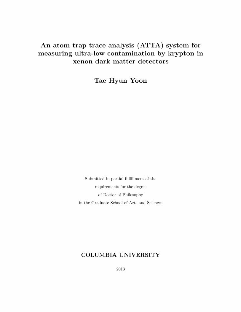
XENON10. A drawing of the XENON100 dark matter detector is shown in Fig. 1.9. The
cylindrical XENON100 TPC of 30.5 cm height and 15.3 cm radius contains an active target
of 65 kg surrounded by 105 kg of LXe active veto. The walls made of 24 panels of polyte-
trafluoroethylene (PTFE, Teflon) circumscribe the cylindrical volume and separate it from
an active LXe veto shield. PTFE is an electrical insulator and a good reflector for the VUV
scintillation light [Yamashita et al., 2004].
XENON100 detects the scintillation signal and the proportional signal using 1 inch
square Hamamatsu R8520-06-Al PMTs, selected for low radioactivity and high quantum
efficiency. The top PMT array where 98 PMTs are held in a concentric PTFE structure
is placed above the target in the xenon gas. The bottom PMT array which consists of 80
PMTs arranged as closely as possible is located below the cathode, immersed in the LXe.
As a LXe dark matter experiment is operated at cryogenic temperatures, a reliable cooling
system with long-term stability is required. For this purpose, XENON100 uses a pulse tube
refrigerator (PTR) Iwatani PC150, driven by a 6.5 kW helium compressor. The cooling
power for this combination is measured to be 200 W at 170 K [Aprile et al., 2012b].
CHAPTER 1. THE XENON EXPERIMENT 14
Figure 1.9: Schematic of the XENON100 dark matter detector. Figure.re from [Aprile et
al., 2012b]

CHAPTER 1. THE XENON EXPERIMENT 15
]2WIMP Mass [GeV/c6 7 8 910 20 30 40 50 100 200 300 400 1000
]2W
IMP-
Nuc
leon
Cro
ss S
ectio
n [c
m
-4510
-4410
-4310
-4210
-4110
-4010
-3910
]2WIMP Mass [GeV/c6 7 8 910 20 30 40 50 100 200 300 400 1000
]2W
IMP-
Nuc
leon
Cro
ss S
ectio
n [c
m
-4510
-4410
-4310
-4210
-4110
-4010
-3910
]2WIMP Mass [GeV/c6 7 8 910 20 30 40 50 100 200 300 400 1000
]2W
IMP-
Nuc
leon
Cro
ss S
ectio
n [c
m
-4510
-4410
-4310
-4210
-4110
-4010
-3910
DAMA/I
DAMA/Na
CoGeNT
CDMS (2010/11)EDELWEISS (2011/12)
XENON10 (2011)
XENON100 (2011)
COUPP (2012)
SIMPLE (2012)
ZEPLIN-III (2012)
CRESST-II (2012)
XENON100 (2012)observed limit (90% CL)
Expected limit of this run:
expectedσ 2 ± expectedσ 1 ±
Figure 1.10: Results on the spin-independent WIMP-nucleon scattering cross section from
XENON100. Figure from [Aprile et al., 2012a]
The data from XENON100 lead to the upper limit on the spin independent WIMP-
nucleon cross section (σSI) with a minimum at 2×10−45 cm2 for a 55 GeV/c2 WIMP mass,
which corresponds to the present best experimental upper limit set on σSI [Aprile et al.,
2012a]. Figure 1.10 describes the results from XENON100 and a set of other experiments
for comparison. The next generation LXe experiment, XENON1T, is currently under con-
struction. XENON1T projects the cross section σSI upper limit of 2.0 × 10−47 cm2 at 50
GeV/c2 with a 2.2 ton LXe target.
1.4 Background in XENON100
1.4.1 Background sources
As XENON100 aims to improve the sensitivity compared to XENON10, the reduction of
the background is critical. In the detector, WIMPs scatter off xenon nuclei and produce low
energy nuclear recoils. Nuclear recoils of similar energy can also be produced by neutrons
passing through the detector, whereas gamma rays and electrons lead to electronic recoils.
As previously mentioned, electronic recoils are distinguished from nuclear recoils via the

CHAPTER 1. THE XENON EXPERIMENT 16
S1/S2 ratio. XENON100 rejects more than 99% of electronic recoils at 50% nuclear recoil
acceptance [Aprile et al., 2010; Aprile et al., 2011]. Despite this rejection efficiency, a
small fraction of electronic recoils may statistically leaks into the nuclear recoil region and
resemble a WIMP signal.
The presence of impurities such as oxygen or other electro-negative impurities in LXe
decreases the size of both S1 and S2 signals. Therefore, xenon in the detector is purified by
recirculating the xenon gas through a high temperature zirconium getter (SEAS MonoTorr
PS3-MT3-R/N-1/2) (Fig. 1.11). While the GXe circulates, impurities in the xenon gas
chemically bond to the getter material and dissipate. LXe extracted from the bottom of
the detector vessel evaporates in the gas line and passes through the getter by a double
diaphragm pump (KNF N143.12E) at a rate of about 5 standard liter per minute (SLPM)
[Aprile et al., 2012b].
Controller
Buffer
Recirculation
Bypass
to Detectorfrom Detector
Port
to Storage
high−TGetter
Pump
Pumping
Flow−
Figure 1.11: Schematic of the XENON100 purification system (left, figure from [Aprile et
al., 2012b]) and image of the gas panel (right). The arrows in the schematic indicate gas
flow in the detector operation.

CHAPTER 1. THE XENON EXPERIMENT 17
During the commissioning phase of XENON100, the detector was heated to 50C, the
temperature limit set by the PMTs, to speed up the purification process before the first
filling with LXe. In the meantime, a residual gas analyzer (RGA) monitored the detector
vacuum. Then the detector was cleaned with hot GXe at a 2 atm pressure, as xenon is
known as a good solvent due to its polarizability [Rentzepis and Douglass, 1981]. The pu-
rification was performed for several weeks by reheating the detector while the warm xenon
gas passed through the getter. During this process, decrease of the water content from ∼500
part per billion (ppb) to 1 ppb level was monitored with a dedicated detector (Tigeroptics
HALO) using the spectral absorption technique [Aprile et al., 2012b].
Energy [keV]0 500 1000 1500 2000 2500 3000
]1
ke
V1
da
y1
Ra
te [
ev
en
ts k
g
410
310
210
data (Fall 2009, no veto cut)
MC (total)
Kr, 120 ppt)85
MC (
Bq/kg)µRn, 21 222MC (
y)2110×=2.111/2
, Tββ νXe 2136
MC (
Pb214
Ac228
Bi214
Bi214
Cs137 Co
60
Co60
K40Tl
208
Tl208
Mn54
Figure 1.12: Energy spectra of the background from measured data and Monte Carlo sim-
ulations in a 30 kg fiducial volume without a veto cut (thick red solid line). Cosmogenic
activation of LXe is not included. The energy spectra of 85Kr and 222Rn decays in LXe
are shown with the thin blue solid and dotted lines, respectively. The thin black dashed
histogram shows the theoretical spectrum of the 2ν double beta decay of 136Xe, assuming
a half-life of 1.1× 10²² years. Figure from [Aprile et al., 2011].
Electronic recoil backgrounds in XENON100 are mainly caused by several sources: ra-
dioactive contamination of the materials of the detector and the shield, intrinsic radioactiv-
ity in the LXe medium, and the decays of 222Rn and its progeny inside the detector shield.
All detector components were selected to minimize the contamination by radioactive mate-
rials. The electronic recoil background of XENON100 is estimated by GEANT4 simulations

CHAPTER 1. THE XENON EXPERIMENT 18
with details of geometry and materials. Figure 1.12 shows the simulated background in a
30 kg fiducial volume with the measured data [Aprile et al., 2010]. In the low energy re-
gion, below 700 keV, the simulated background shows good agreement with the measured
background.
While the background stemming from radioactive materials in the detector and shield
materials can be reduced by a fiducial volume cut, the intrinsic background from radioactive
isotopes in the LXe is a fundamental limitation to the experiment sensitivity. Table 1.2
presents predicted electronic recoils from the detector and shield materials and the intrinsic
radioactive impurities in the energy region of interest. In the 30 kg fiducial volume, 85Kr
contributes∼30% to the total background without veto cut and 55% when a veto coincidence
is applied below a threshold energy of 100 keV. In other words, 85Kr becomes the dominant
source of the electronic recoil background after selecting an optimized fiducial volume and
an active veto cut [Aprile et al., 2011].
Table 1.2: Summary of the predicted electronic recoil background: rate of single scatter
events in the energy region below 100 keV, before S2/S1 discrimination. The veto cut with
an average energy threshold of 100 keV has been applied. Table from [Aprile et al., 2011].
Predicted rate [×10−3 events·kg−1·day−1·keV−1]
Volume 62 kg target 40 kg fiducial 30 kg fiducial
Veto cut none active none active none active
Detector and shield materials 137.22 75.30 12.89 3.42 7.22 2.02
222Rn in the shield (1 Bq/m3) 5.95 1.72 0.92 0.16 0.16 0.02
85Kr in LXe (150 ppt of natKr) 2.90 2.90 2.90 2.90 2.90 2.90
222Rn in LXe (21 µBq/kg) 1.04 0.51 0.56 0.38 0.53 0.37
All sources 147.11 80.43 17.27 6.86 10.81 5.31
1.4.2 Removal of 85Kr from xenon
Radioactive decay of 85Kr results in beta particle, with maximum energy of 687 keV, and
this is the major source of electronic recoils in XENON100 as discussed in Sec. 1.4.1. 85Kr

CHAPTER 1. THE XENON EXPERIMENT 19
is artificially created in nuclear fission, and makes up ∼ 10−11 of the total krypton isotopes.
The properties of krypton and specifically 84Kr will be discussed in more detail in Sec. 2.2.
Xenon gas extracted from the atmosphere contains krypton impurities at a part per million
(ppm) level after distillation and absorption-based chromatography.
E [keVee]1 10 210 310
Rat
e [e
vent
s/kg
/keV
ee/d
ay]
-1110
-1010
-910
-810
-710
-610
-510
-410
-310
-210
-110, 50% efficiency) 2 cm-45=2x10
SIσWIMP (M=50GeV,
, 50% efficiency) 2 cm-47=5x10SI
σWIMP (M=50GeV,
100 ppt Kr/Xe (after 99.5% rejection)
1 ppt Kr/Xe (after 99.5% rejection)
Figure 1.13: Differential scattering rates of weakly interacting massive particles (WIMPs)
and decay rates of 85Kr for XENON100 and XENON1T sensitivity goals.
The xenon gas used for XENON100 has been purified by a commercial cryogenic distil-
lation plant (Spectra Gases Co.) to reduce the krypton concentration level to ∼ 10 ppb.
This concentration level still needs to be reduced by a factor of 100 as krypton impuri-
ties at the 100 part per trillion (ppt) level in the xenon gas would contribute a rate of
∼ 2 × 10⁻³ events × kg × keVee−1 × day−1 from 85Kr [Aprile et al., 2011]. The expected
rates of WIMP events for XENON100 and XENON1T are shown in Fig. 1.13, along with
the rates of electronic recoils due to 85Kr. The blue solid line indicates the Kr/Xe level
required to achieve the projected sensitivity of the XENON100 experiment, 100 ppt, and
the green dashed line presents that for XENON1T, 1 ppt.
As XENON100 is the first low background experiment using a large quantity of LXe, a

CHAPTER 1. THE XENON EXPERIMENT 20
Figure 1.14: Cryogenic distillation column used to separate krypton (left, figure from [Aprile
et al., 2012b]) and an image of the setup (right). The XENON column has a height of about
3 m.
krypton contamination at ultra-low levels is critical to the sensitivity of the experiment. In
order to further reduce krypton impurities in the xenon, a small-scale cryogenic distillation
column was integrated into the XENON100 system underground. The column is designed
to reduce the krypton concentration by a factor of 1000 in a single pass, at a purification
speed of 1.8 SLPM (or 0.6 kg/h). A schematic and an image of the cryogenic distillation
column are shown in Fig. 1.14. The xenon gas is cooled using a cryocooler before entering
the column at half height. A thermal gradient is kept constant using a heater at the bottom
of the column and a cryocooler at the top. Due to the different boiling temperatures of
krypton (120 K at 1 atm) and xenon (165 K), a krypton-enriched mixture stays at the top
of the column and a krypton-depleted one at the bottom. The high krypton concentration
xenon is separated by freezing it into a gas bottle, and the purified xenon at the bottom is
used for the experiment [Lim, 2013].
After installation and the initial commissioning run of the new column, the second

CHAPTER 1. THE XENON EXPERIMENT 21
distillation of the full xenon inventory was performed in the summer of 2009. For the
commissioning run, the krypton concentration in xenon was measured with a delayed coin-
cidence analysis at 143+135−90 ppt (90% CL) [Aprile et al., 2010], which agrees with the value
inferred from a comparison of the measured background spectrum with a Monte Carlo sim-
ulation [Aprile et al., 2011]. In the second science run [Aprile et al., 2012a], the krypton
contamination was lowered to (19 ± 4 ppt), measured by ultrasensitive rare gas mass spec-
troscopy. This agrees with the value (18 ± 8 ppt) derived from the analysis of delayed β-γ
coincidences associated with the 85Kr beta decay. The krypton contamination of xenon
samples, recently drawn from the XENON100 detector, was measured to be below 1 ppt
from a mass spectroscopic technique [Lindemann and Simgen, 2013].
CHAPTER 2. ATOMIC PROPERTIES 22
Chapter 2
Atomic properties
This work aims to determine the ppt-level contamination by krypton in the xenon sample
from the XENON dark matter experiment. Argon gas is used to avoid contamination by
krypton for the testing phase. The three relevant elements, argon, krypton, and xenon, are
noble gases with a full outer shell of valence electrons in the ground state, leading to several
common properties. Prior to describing the atom trap trace analysis (ATTA) system, the
properties of these elements are presented in this chapter.
2.1 Argon
Argon, whose atomic number is 18, was discovered by Lord Rayleigh and Sir William Ram-
say in 1894. Argon exists in a gas phase at standard temperature and pressure (STP) with
the melting point of 83.80 K and the boiling point of 87.30 K at 1 atm. It is the third most
common gas in air, making up 0.93% of the earth’s atmosphere [Haynes, 2013]. Argon has 3
stable and 21 unstable isotopes with the electron configuration of 1s22s22p63s23p6. Table 2.1
describes physical properties of argon and the abundances of its selected isotopes. Argon
is inert and it is not known to form any stable compounds at room temperature [Haynes,
2013]. Table 2.2 displays some excited states of argon and their electronic configurations
with energies, and the energies of each state are also drawn in Fig. 2.1.
Argon is produced industrially by the fractional distillation of liquid air, and is widely
used where an inert gas is needed since it is the most abundant and cheapest noble gas.

CHAPTER 2. ATOMIC PROPERTIES 23
Table 2.1: Physical properties of argon.
Property Value
Atomic number Z 18
Molar mass 39.948 g mol−1
Isotopic properties 36Ar (0.337 %, stable), 38Ar (0.063 %, stable)
39Ar (trace, β− decay, t1/2=35 d)
40Ar (99.6 %, stable)
41Ar (synthetic, β− decay, t1/2 = 109.34 min)
Gas density (273.15 K, 1 atm) 1.784 g cm−3
Liquid density (87.30 K, 1 atm) 1.40 g cm−3
Melting point (1 atm) 83.80 K
Boiling point (1 atm) 87.30 K
Triple point 83.81 K, 0.68 atm, 3.08 g cm−3
Critical point 150.87 K, 48.34 atm, 1.155 g cm−3
The property of plasma discharge makes argon used in electric light bulbs and in fluorescent
tubes based on plasma discharge. It is also used in arc welding and cutting to protect the
weld or cut area from atmospheric contamination. In scientific applications, some direct
dark matter searches such as ArDM use argon as the target material to interact with weakly
interacting massive particles (WIMPs).
2.1.1 40Ar
As mentioned in the first part of this chapter, we use 40Ar for testing and optimizing the
system before detecting 84Kr in the xenon sample. 40Ar, containing 18 protons and 22
neutrons, is the most common isotope (99.6% of all argon in nature), and has an atomic
mass of 39.9624. This isotope is produced via decay of 40K, which is a radioactive isotope
of potassium with a half-life of 1.25 × 10⁹ years. About 88.8% of the time, naturally
occurring 40K transforms to stable 40Ca by emitting a β particle and an antineutrino. In
the other cases (11.2%), it decays to stable 40Ar by electron capture with a gamma ray

CHAPTER 2. ATOMIC PROPERTIES 24
Energy Levels of Argon
Energy [eV]
0
12.
13.
Singlet Triplet
s p s p
1S
2P3/24s[3/2]1
2P1/24s[1/2]1
2P3/24p[5/2]2
2P3/24p[3/2]2
2P3/24p[1/2]0
2P3/24s[3/2]2
2P1/24s[1/2]0
2P3/24p[3/2]2
2P3/24p[5/2]3
2P3/24p[1/2]0
1.527361 eV
Figure 2.1: Grotrian diagram of argon. The black arrow indicates the transition used for
cooling and trapping.

CHAPTER 2. ATOMIC PROPERTIES 25
Table 2.2: Energy levels of neutral argon.
Electron Configuration Spin Configuration 2S+1Ljnl[K]J Energy [eV]
3s23p6 0
3s23p54s1 triplet 2P3/24s[3/2]2a 11.548354
3s23p54s1 singlet 2P3/24s[3/2]1 11.623592
3s23p54s1 triplet 2P1/24s[1/2]0 11.723160
3s23p54s1 singlet 2P1/24s[1/2]1 11.828071
3s23p54p1 triplet 2P3/24p[1/2]1 12.907015
3s23p54p1 singlet 2P3/24p[1/2]0 13.273038
3s23p54p1 triplet 2P3/24p[5/2]3a 13.075715
3s23p54p1 singlet 2P3/24p[5/2]2 13.094872
3s23p54p1 singlet 2P3/24p[3/2]2 13.153143
3s23p54p1 triplet 2P3/24p[3/2]1 13.171777
a Transition between these two levels is used for cooling and detection.
and a neutrino or rarely by emitting a position and a neutrino. This decay ratio is used to
determine radiometric dates for geological events [McDougall, 1999].
2.2 Krypton
Krypton is an element in the group of noble gases, with an atomic number 36. Ramsay
and Travers discovered krypton in 1898 in the residue left after liquid air had nearly boiled
away [Haynes, 2013]. Krypton is present in the air at the ∼1 ppm level, and has 6 stable
isotopes and 30 unstable isotopes. Table 2.3 shows physical properties of krypton with a
list of selected isotopes. Ground state krypton has an electron configuration of 3d104s24p6
containing that of the ground state argon. The configurations of several excited states and
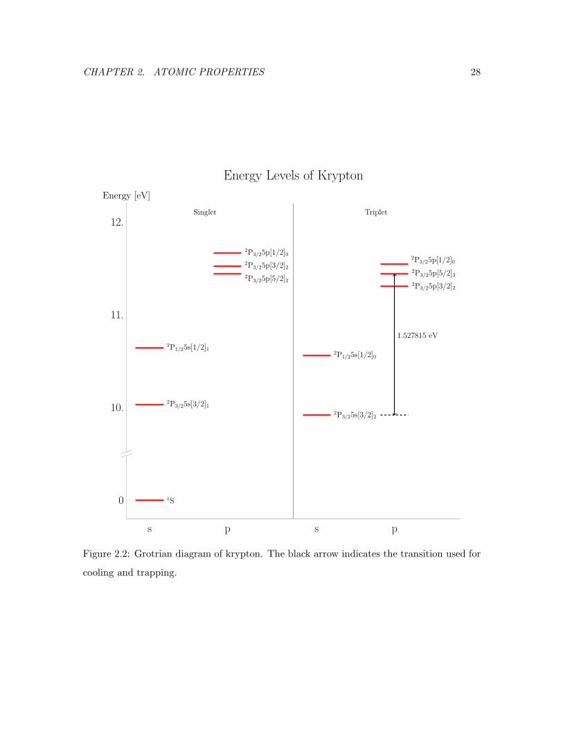
their energies are listed in Tab. 2.4, and Fig. 2.2 shows the energy diagram.
Krypton, characterized by its several sharp emission lines including the brilliant green
and orange, is used in lighting like other noble gases. Ionized krypton gas discharges appear
whitish due to its multiple emission lines. Using this feature, krypton can be used in

CHAPTER 2. ATOMIC PROPERTIES 26
Table 2.3: Physical properties of krypton.
Property Value
Atomic Number Z 36
Molar mass 83.798 g mol−1
Isotopic Abundance 78Kr (0.35 %, β+ decay, t1/2 > 1.1× 10²⁰ y)
79Kr (0.35 %, ǫ β+ γ decay, t1/2 = 35.04 h)
80Kr (2.25 %, stable)
81Kr (trace, ǫ γ decay, t1/2 = 2.29 × 10⁵ y)
82Kr (11.6 %, stable)
83Kr (11.5 %, stable)
84Kr (57.0 %, stable)
85Kr (trace, β− decay, t1/2 = 10.765 y)
86Kr (17.3 %, stable)
Gas density (273 K, 1 atm) 3.749 g cm−3
Liquid density (165.05 K, 1 atm) 2.413 g cm−3
Melting point (1 atm) 115.79 K
Boiling point (1 atm) 119.93 K
Triple point 115.775 K, 0.722 atm, 3.08 g cm−3
Critical point 209.42 K, 54.28 atm, 1.155 g cm−3

CHAPTER 2. ATOMIC PROPERTIES 27
photographic projection lamps as a brilliant white light source. The relative abundance of
krypton versus hydrogen can be used by astronomers to measure how much nucleosynthesis
has taken place in any region of interstellar space [Cartledge et al., 2008]. One of the
stable isotopes, 86Kr, was used for definition of the fundamental unit of length. In 1960,
the General Conference on Weights and Measures (Confrence Gnrale des Poids et Mesures,
CGPM) defined the meter based on the wavelength of 86Kr radiation. (In 1983, it was
replaced with the length of the path traveled by light in vacuum during a time interval of
1/299,792,458 s [Taylor and Thompson, 2008].)
Table 2.4: Energy levels of neutral krypton.
Electron Configuration Spin Configuration 2S+1Ljnl[K]J Energy [eV]
4s24p6 0
4s24p55s1 triplet 2P3/25s[3/2]2a 9.915231
4s24p55s1 singlet 2P3/25s[3/2]1 10.032400
4s24p55s1 triplet 2P1/25s[1/2]0 10.562413
4s24p55s1 singlet 2P1/25s[1/2]1 10.643634
4s24p55p1 triplet 2P3/25p[1/2]1 11.303454
4s24p55p1 singlet 2P3/25p[1/2]0 11.666027
4s24p55p1 triplet 2P3/25p[5/2]3a 11.443046
4s24p55p1 singlet 2P3/25p[5/2]2 11.444655
4s24p55p1 singlet 2P3/25p[3/2]2 11.526115
4s24p55p1 triplet 2P3/25p[3/2]1 11.545822
a Transition between these two levels is used for cooling and detection.
2.2.1 85Kr
85Kr, containing 49 neutrons and 36 protons, is produced mainly by fission of uranium and
plutonium in nuclear reactors and released during chopping and dissolution of fuel rods in
nuclear reprocessing, and the interaction of cosmic rays with stable 84Kr also generates a
small quantity of 85Kr. Currently, artificially produced 85Kr overwhelms the cosmogenic
CHAPTER 2. ATOMIC PROPERTIES 28
Energy Levels of Krypton
Energy [eV]
0
10.
11.
12.Singlet Triplet
s p s p
1S
2P3/25s[3/2]1
2P1/25s[1/2]1
2P3/25p[5/2]2
2P3/25p[3/2]2
2P3/25p[1/2]0
2P3/25s[3/2]2
2P1/25s[1/2]0
2P3/25p[3/2]2
2P3/25p[5/2]3
2P3/25p[1/2]0
1.527815 eV
Figure 2.2: Grotrian diagram of krypton. The black arrow indicates the transition used for
cooling and trapping.

CHAPTER 2. ATOMIC PROPERTIES 29
production of 85Kr. This isotope is the most abundant man-made radioisotope in the
troposphere [Schroder et al., 1971]. 85Kr, once released into the atmosphere, diminishes
only via radioactive decay where it transforms into 85Rb with a half-life of 10.76 years and
a maximum energy of 0.687 MeV (Tab. 2.3). The global atmospheric content has been
continuously increasing since the installation of reprocessing plants for nuclear fuel in the
early 1950s and reached 5.5×10¹⁵ Bq at the end of 2009 [Ahlswede et al., 2013]. Figure 2.3
shows the increase of the global 85Kr inventory with time. The current isotopic abundance
of 85Kr in the atmosphere is at the level of 10−11.
Figure 2.3: Global accumulated 85Kr inventory (radioactive decay accounted for) and the
annual emissions. The emissions unit is PBq = 1015 Bq = 1015 s−1. Figure from [Ahlswede
et al., 2013].
The radioactive properties of 85Kr, combined with accumulated data of its global ob-
servations since the 1950s, allow us use the isotope as a tracer in environmental samples.
Researchers use 85Kr to estimate the age of young groundwater (< 40 years). For a ground-
water system with small dispersion, the age of groundwater can be estimated directly from
85Kr activity [Ekwurzel et al., 1994]. Global observation of 85Kr is used to calibrate and
examine atmospheric transport models [Levin and Hesshaimer, 1996], and a temporal and
CHAPTER 2. ATOMIC PROPERTIES 30
spatial concentration of 85Kr gives an indication of a nuclear leak accident or an undeclared
plutonium stockpile [Hippel et al., 1985].
85Kr has several industrial applications. For example, 85Kr is allowed to diffuse into
extremely small cracks, where the atoms are trapped and detected by normal photographic
techniques. This method is called krypton gas penetrant imaging [Glatz, 1996]. Another
usage of 85Kr is as an additive in arc discharge lamps. It is known that the presence of 85Kr
in discharge tubes makes the lamps easy to ignite by reducing their starting voltage [Linde
Electronics and Specialty Gases, 2010].
2.2.2 84Kr
84Kr is the most abundant krypton isotope with the natural abundance of 57%. In this
experiment, 84Kr is detected to take advantage of its large abundance. 84Kr is stable and
thus has no decay products. It contains 48 neutrons and 36 protons, which leads to the
atomic mass of 83.9115.
2.3 Xenon
Xenon, a heavy noble gas with an atomic number of 54, was first found by Ramsay and
Travers in 1898 in the residue left after evaporating liquid air components. Xenon is a
colorless, odorless monatomic gas under STP as the other noble gases. It is present at
about one part in twenty million in the atmosphere [Haynes, 2013]. Xenon consists of 9
stable isotopes and 35 unstable isotopes that radioactively decay. Physical properties of
xenon and its isotopes are summarized in Tab. 2.5. Though Xe gas is generally inert, a
few chemical reactions are known such as the formation of xenon hexafluoroplatinate, the
product of platinum hexafluoride and xenon [Bartlett, 1962]. The electron configuration of
the ground state xenon is 5s24d105p6 containing that of the ground state krypton. Xenon
is obtained as a byproduct of the separation of air into oxygen and nitrogen. The resulting
liquid oxygen mixture contains both krypton and xenon, which are extracted by fractional
distillation, and at the last stage, xenon is extracted from the krypton-xenon mixture by
distillation. The typical price of xenon is about 1000 $/kg; its rarity makes it much more

CHAPTER 2. ATOMIC PROPERTIES 31
expensive than other noble gases [Plante, 2012].
Table 2.5: Physical properties of xenon. Table from [Plante, 2012].
Property Value
Atomic Number Z 54
Molar mass 131.29 g mol−1
Isotopic Abundance 124Xe (0.095%, β+ decay, t1/2 > 4.8× 10¹⁶ y)
126Xe (0.89%, stable), 129Xe (26.4%, stable)
130Xe (4.07%, stable), 131Xe (21.2%, stable)
132Xe (26.9%, stable)
134Xe (10.4%, β− decay, t1/2 > 1.1× 10¹⁶ y)
136Xe (8.86%, β− decay, t1/2 = 2.11 × 10²¹ y)
Gas density (273.15 K, 1 atm) 5.8971 g cm−3
Liquid density (165.03 K, 1 atm) 3.057 g cm−3
Melting point (1 atm) 161.4 K
Boiling point (1 atm) 165.03 K
Triple point 161.31 K, 0.805 atm, 3.08 g cm−3
Critical point 289.74 K, 57.65 atm, 1.155 g cm−3
Xenon has a number of applications despite its high price. Xenon excited by an electrical
discharge creates a characteristic blue glow. It is used in gas-discharge lamps such as xenon
flash lamps, arc lamps, and plasma displays. Xenon-containing dimers (Xe2, XeCl, XeF,
etc.) are used in excimer lasers to provide stimulated emission. In science, xenon is used in
calorimeters for measurements of gamma rays and as a medium for dark matter searches
such as XENON and LUX.

CHAPTER 3. BASIC CONCEPTS 32
Chapter 3
Basic concepts
In this experiment, we cool and trap atoms of interest to count their number in a given
quantity of carrier atoms. Standard cooling and trapping methods used here are based
on the interaction between light and nearly two-level atoms. In this chapter, we review
the basic principle of light-atom interaction and the details of each cooling and trapping
techniques: transverse cooling, Zeeman slowing, and magneto-optical trapping.
3.1 Light forces on atoms
An atom in the presence of light can be described by the time-dependent Schrodinger
equation
ih∂Ψ
∂t= HΨ, (3.1)
where H is the Hamiltonian operator. The Hamiltonian has the time independent field-free
atomic part, H0, and the time dependent atom-light interaction part, HI . Thus, H =
H0 +HI .
For a two-level atom and no external field, the Hamiltonian is time independent in the
Schrodinger picture, and the Schrodinger equations for each level are
H0ψ1(~r) = E1ψ1(~r),
H0ψ2(~r) = E2ψ2(~r),(3.2)
where E1 and E2 are the energies of the levels. Then we can express the wavefunction time

CHAPTER 3. BASIC CONCEPTS 33
evolution as
Ψ(~r, t) = c1 ψ1(~r) e−iE1t/h + c2 ψ2(~r) e
−iE2t/h
= c1 |1〉 e−iω1t + c2 |2〉 e−iω2t, (3.3)
where ω1 = E1/h and ω2 = E2/h.
An electric field ~E due to the light produces the perturbation term
HI = −~d · ~E, (3.4)
where ~d is the electric dipole moment ~d = −e ~r. From this Hamiltonian, the Rabi frequency
Ω is defined as
Ω =〈2|~d · ~E|1〉
h. (3.5)
Now, we introduce the density matrix
ρ = |Ψ〉〈Ψ| =(c1c2
)(c∗1 c∗2
)=
ρ11 ρ12
ρ21 ρ22
. (3.6)
The diagonal elements ρ11 and ρ22 are the populations of the states |1〉 and |2〉. The off-
diagonal elements, called coherences, represent the response of the system at the driving
frequency. Then Eq. 3.1 can be written as
ihdρ
dt= [H, ρ] . (3.7)
For convenience, we define new variables
u = ρ12 + ρ21,
v = −i(ρ12 − ρ21),
w = ρ11 − ρ22,
(3.8)
where ρ12 ≡ ρ12 exp(−iδt) and ρ21 ≡ ρ21 exp(iδt). Here, δ = ωl − ω0 is the detuning of the
light, ωl is the light frequency, and ω0 = (E2 − E1)/h is the atomic transition frequency.
The atoms in the excited state decay to the ground state and emit photons, both via
stimulated and spontaneous emission. The process of spontaneous emission can be in-
troduced phenomenologically as ρ22(t) = ρ22 exp(−Γt), where Γ is the atomic transition

CHAPTER 3. BASIC CONCEPTS 34
linewidth. Equation 3.1 with the effect of spontaneous emission yields the following equa-
tions:
u = δv − Γ
2u,
v = −δu+Ωω − Γ
2v,
w = −Ωv − Γ(ω − 1).
(3.9)
These are the optical Bloch equations. For the steady state case (t ≫ Γ−1), their solution
is
u
v
w
=
1
δ2 +Ω2 + Γ2/4
Ωδ
ΩΓ/2
δ2 + Γ2/4
(3.10)
By inserting this solution into the definition of w in Equation 3.8, we can derive the popu-
lation ρ22 of the excited state,
ρ22 =1− w
2=
Ω2/4
δ2 +Ω2 + Γ2/4
=1
2
I/Isat1 + I/Isat + (2δ/Γ)2
. (3.11)
In the second line of Equation 3.11 we introduced a new variable, the saturation intensity
Isat, which is defined asI
Isat=
2Ω2
Γ2≡ s0, (3.12)
where s0 is the on-resonance saturation parameter.
Now we can obtain an expression for the photon scattering rate in atom-light interac-
tions. The scattering rate is expressed as
Rscatt = Γρ22 =Γ
2
s01 + s0 + (2δ/Γ)2
. (3.13)
When a ground state atom absorbs a photon and is excited to an upper energy level,
the momentum of the photon is transferred to the atom, and the atom receives a kick in
the direction of the photon’s propagation. When the excited atom returns to the original
state via stimulated emission, the emitted photon has the same direction as the absorbed
photon, and as a result, the overall momentum change of the atom during this cycle is zero.
When the excited atom decays via spontaneous emission, however, a photon is emitted in
CHAPTER 3. BASIC CONCEPTS 35
a random direction. Therefore, the momentum change due to spontaneous emissions will
cancel out, and only effects from photon absorption are accumulated after a large number of
cycles. This results in the scattering force, and its magnitude is a product of the incoming
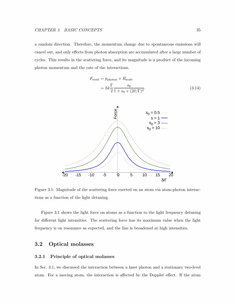
photon momentum and the rate of the interactions.
Fscatt = pphoton ×Rscatt
= hkΓ
2
s01 + s0 + (2δ/Γ)2
. (3.14)
-20 -15 -10 -5 0 0 5 10 15 20
For
ce
δ/Γ
s0 = 0.5s = 1
s0 = 3s0 = 10
Figure 3.1: Magnitude of the scattering force exerted on an atom via atom-photon interac-
tions as a function of the light detuning.
Figure 3.1 shows the light force on atoms as a function to the light frequency detuning
for different light intensities. The scattering force has its maximum value when the light
frequency is on resonance as expected, and the line is broadened at high intensities.
3.2 Optical molasses
3.2.1 Principle of optical molasses
In Sec. 3.1, we discussed the interaction between a laser photon and a stationary two-level
atom. For a moving atom, the interaction is affected by the Doppler effect. If the atom

CHAPTER 3. BASIC CONCEPTS 36
is moving toward the light source with velocity v (Fig. 3.2), the frequency of the laser
appears blue-shifted to the atom, ωl → ωl + kv. In other words, the atomic resonance
appears at ω0 → ω0 − kv to the photon. We take the latter notation in the rest part of this
thesis. The Doppler effect modifies the scattering force Fscatt(ωl−ω0) to Fscatt(ωl−ω0+kv).
ωl
Incident lightTwo-level atom
ω0
v
Figure 3.2: Schematic of atom-photon interaction for an atom moving toward the light
source.
Optical molasses are set up by two counterpropagating laser beams that have the same
frequency and intensity. When an atom moves with velocity v along the light propagation
axis, the net force on the atom is expressed as the sum of the scattering forces from each
laser,
Fmolasses = Fscatt(ωl − ω0 − kv)− Fscatt(ωl − ω0 + kv). (3.15)
For a low velocity condition, satisfying kv ≪ Γ, this equation can be rewritten as
Fmolasses ≃[Fscatt(ωl − ω0)− kv
∂F
∂ω
]−[Fscatt(ωl − ω0) + kv
∂F
∂ω
]
= −2∂F
∂ωkv. (3.16)
We define a new coefficient
α ≡ 2k∂F
∂ω= 4hk2s0
−2δ/Γ
[1 + s0 + (2δ/Γ)2]2. (3.17)
Then Eq. 3.16 is written in the form
Fmolasses = −αv, (3.18)
where α is an effective damping coefficient that is analogous to a mechanical viscous damper
in a damped harmonic oscillator setup.

CHAPTER 3. BASIC CONCEPTS 37
For
ce
Velocity
Figure 3.3: Optical molasses force as a function of atom velocity along the axis of light
propagation. Blue lines are forces due to each counterpropagating light beam, and the
green line is the net force.
Figure 3.3 shows the force exerted on an atom in optical molasses as a function of
the atom’s velocity. We see that the net force (green line) is almost linear in the small
velocity region as Eq. 3.18 indicates. The force grows with velocity in this region. Beyond
a certain threshold velocity, however, the net force falls and the optical molasses does not
work properly.
3.2.2 The Doppler limit of optical molasses
The concept discussed in Sec. 3.2.1 seems to imply that any atoms with small velocities
can be cooled to the absolute zero. In reality, however, this does not happen. Concomitant
heating in the optical molasses prevents the atoms from cooling down below a certain
temperature. In this section, we estimate the temperature limit of one dimensional optical
molasses at low light intensities.
When momentum is transferred from a photon to an atom or vice versa, not only the

CHAPTER 3. BASIC CONCEPTS 38
atomic momentum but also ts energy changes. The energy change equals the recoil energy
Erecoil =p2photon2M
=h2k2
2M, (3.19)
whereM is the atomic mass. The recoil energy occurs for both absorption and spontaneous
emission, hence the atom will gain an energy of 2Erecoil in each scattering event. Since the
scattering rate from two beams is 2Rscatt, the overall heating rate becomes 4RscattErecoil.
From Newton’s second law of motion, the cooling rate in optical molasses is expressed
asd
dt(1
2Mv2) =Mv
dv
dt= −αv2 = vFmolasses. (3.20)
The cooling rate should be same as the heating rate in steady state. From this condition,
we obtain the relation
vFmolasses = 4RscattErecoil,
4hk2s02|δ|/Γ
[1 + s0 + (2δ/Γ)2]2v2 = 4
h2k2
2M
Γ
2
s01 + s0 + (2δ/Γ)2
. (3.21)
Evaluation of Eq. 3.21 yields the kinetic energy of the atom
Ekinetic =hΓ
8(2|δ|Γ
+Γ
2|δ| ). (3.22)
The on-resonance saturation parameter s0 has been neglected here since we deal with only
the low intensity case, s0 = I/Isat ≪ 1. Equation 3.22 has its minimum value of hΓ/4 at
δ = Γ/2. We use the equipartition theorem 12Mv2 = 1
2kBTD to derive the temperature
corresponding to this kinetic energy,
TD =hΓ
2kB, (3.23)
where kB is the Boltzmann constant. The Doppler cooling limit or Doppler temperature TD
indicates the lowest temperature that can be achieved with optical molasses [Foot, 2005].
For electric-dipole atomic transitions, typical TD values are sub-millikelvin [Metcalf and
van der Straten, 1999]. For example, by inserting the linewidth of 84Kr 5.56 MHz, into
Eq. 3.23, we evaluate the Doppler temperature TD = 133.4 µK, which corresponds to the
atomic velocity v = 11.5 cm/s from the equipartition theorem.

CHAPTER 3. BASIC CONCEPTS 39
3.3 Zeeman slowing
For decelerating a one dimensional atomic beam, one can simply use a counter propagating
light beam. The light frequency should be red-shifted to match the Doppler shift due to the
atoms’ velocity. This method works well for atoms with a narrow velocity range, but has
its limit in that the magnitude of the Doppler effect changes as atoms are slowed. Different
light frequencies are required for the different atom velocities. This can be accomplished
by sweeping the laser frequency rapidly, which is called the chirp cooling [Prodan and
Phillips, 1984]. This method has an obvious disadvantage that slowed atoms arrive in
pulses separated by the sweeping period. W. Phillips and H. Metcalf came up with an
ingenious way to solve this problem using a spatially varying magnetic field [Phillips and
Metcalf, 1982].
In the presence of a magnetic field ~B, the Hamiltonian for a free atom is
H = H0 +HB . (3.24)
HB is a perturbation Hamiltonian from the magnetic field,
HB = −~µ · ~B, (3.25)
where ~µ is the magnetic moment of the atom. This perturbation shifts the atomic transition
energy by ∆E = µ′B. In other words, the effective transition frequency changes as ω0 →ω0+µ
′B/h. µ′ is the effective magnetic moment for the transition, defined as µ′ ≡ (g2M2−g1M1)µB, where µB is the Bohr magneton, g1,2 is the Lande g-factor, and M1,2 is the
magnetic quantum number. The splitting of a spectral line due to the energy shifts by a
magnetic field is the Zeeman effect. In this context, let us consider the case of a Zeeman
slower with a red-detuned light. Then the term µ′B/h is required to be negative, which is
accomplished by a transition with ∆M = −1.
A varying magnetic field B along the atomic beam axis shifts the transition frequency
so that the Zeeman effect compensates for the change of Doppler shift. This apparatus
is known as a Zeeman slower. The varying magnetic field is traditionally achieved by
a tapered solenoid, and recently an apparatus using permanent magnets was developed
[Ovchinnikov, 2008; Reinaudi et al., 2012]. Taking into account the effect of this magnetic

CHAPTER 3. BASIC CONCEPTS 40
field and the Doppler effect from varying velocities, we obtain a modified scattering force
FZS(ωl − ω0 + kv(z) − µ′B(z)/h). This means that the Zeeman shift by the magnetic field
should obey the condition
ω0 = ωl + kv(z)− µ′B(z)
h. (3.26)
Figure 3.4 (top) shows this relation for the atomic energy level, as well as the working
principle of a Zeeman slower. Figure 3.4 (bottom) is a schematic of the apparatus.
hωl z
Energy
|µ′B(z)|
kv(z)
hω0xxxxxxxxxxxxxxxxxxxxxxxxxxxxxxxxxxxxxxxxxxxxxxxxxxxxxxxxxxxxxxxxxxxxxxxxxxxxxxxxxxxxxxxxxxxxxxxxxxxxxxxxxxxxxxxxxxxxxxxxxxxxxxxxxxxxAtomicbeam Red shifted
laser
Tapered solenoid
Figure 3.4: Diagram of the energy level in a Zeeman slower (top) and schematic of the
apparatus using tapered solenoid to produce the varying magnetic field (bottom). As an
atom is decelerated, the Doppler shift decreases and the larger Zeeman effect compensates
for this decrease.
From Newtonian mechanics, the velocity at position z satisfies the relation v20 − v(z)2 =
2az, where v0 is the initial velocity at the entrance of the Zeeman slower. For the constant
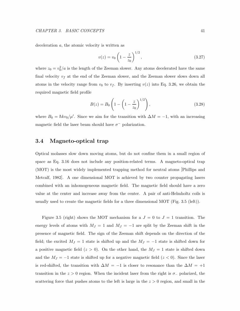
CHAPTER 3. BASIC CONCEPTS 41
deceleration a, the atomic velocity is written as
v(z) = v0
(1− z
z0
)1/2
, (3.27)
where z0 = v20/a is the length of the Zeeman slower. Any atoms decelerated have the same
final velocity vf at the end of the Zeeman slower, and the Zeeman slower slows down all
atoms in the velocity range from v0 to vf . By inserting v(z) into Eq. 3.26, we obtain the
required magnetic field profile
B(z) = B0
(1−
(1− z
z0
)1/2), (3.28)
where B0 = hkv0/µ′. Since we aim for the transition with ∆M = −1, with an increasing
magnetic field the laser beam should have σ− polarization.
3.4 Magneto-optical trap
Optical molasses slow down moving atoms, but do not confine them in a small region of
space as Eq. 3.16 does not include any position-related terms. A magneto-optical trap
(MOT) is the most widely implemented trapping method for neutral atoms [Phillips and
Metcalf, 1982]. A one dimensional MOT is achieved by two counter propagating lasers
combined with an inhomogeneous magnetic field. The magnetic field should have a zero
value at the center and increase away from the center. A pair of anti-Helmholtz coils is
usually used to create the magnetic fields for a three dimensional MOT (Fig. 3.5 (left)).
Figure 3.5 (right) shows the MOT mechanism for a J = 0 to J = 1 transition. The
energy levels of atoms with MJ = 1 and MJ = −1 are split by the Zeeman shift in the
presence of magnetic field. The sign of the Zeeman shift depends on the direction of the
field; the excited MJ = 1 state is shifted up and the MJ = −1 state is shifted down for
a positive magnetic field (z > 0). On the other hand, the MJ = 1 state is shifted down
and the MJ = −1 state is shifted up for a negative magnetic field (z < 0). Since the laser
is red-shifted, the transition with ∆M = −1 is closer to resonance than the ∆M = +1
transition in the z > 0 region. When the incident laser from the right is σ− polarized, the
scattering force that pushes atoms to the left is large in the z > 0 region, and small in the

CHAPTER 3. BASIC CONCEPTS 42
y
x
z
I
I
+
−
σ−
σ+
σ+
σ−
z
Energy
BB
0 0
-1
-11
1
σ+
σ−
MJMJ
J = 1
J = 0
ωlω0
Figure 3.5: Schematic of a three dimensional magneto-optical trap (MOT) (left), and prin-
ciple of one dimensional MOT (right).
z < 0 region. Similarly, the σ+ polarized laser from the left pushes atoms in the z < 0
region more than atoms in the z > 0 region. The imbalance of these forces drives atoms to
the center of the trap.
The scattering force with the Zeeman effect and the Doppler shift is FZS(ωl −ω0+ kv+
µ′B/h), same as for a Zeeman slower. In a one dimensional MOT, the forces from two
counter propagating lasers lead to the net force on the atoms;
FMOT = F σ+
scatt(ωl − ω0 − kv +µ′B
h)− F σ−
scatt(ωl − ω0 + kv − µ′B
h) (3.29)
When the magnetic field is a linear function of the position, B(z) = Az, this equation
becomes
FMOT = F σ+
scatt(ωl − ω0 − kv(z) +µ′
hAz)− F σ−
scatt(ωl − ω0 + kv − µ′
hAz)
≃ −2∂F
∂ωlkv + 2
∂F
∂ω0
µ′
hAz
= −2∂F
∂ωl(kv +
µ′
hAz)
= −βv − κz, (3.30)
where β ≡ 2(∂F/∂ωl)k and κ ≡ βµ′A/kh. In the third line, we used the relation ∂F/∂ωl =
−∂F/∂ω0, since δ = ωl−ω0. The last line has the form of a harmonic oscillator force, where

CHAPTER 3. BASIC CONCEPTS 43
β is the viscous damping coefficient, and κ is the spring constant. The first term reduces
the atom velocity and the second term confines the atoms in the center of the trap.
Typically, a MOT collects atoms prepared by a Zeeman slower for a high loading rate.
The capture velocity of a MOT - the maximum atom velocity that the MOT can trap -
can be estimated from the maximum FMOT and the trap laser beam diameter d using the
equation v20 − v2f = 2as, where s is the displacement:
v2c = 2FMOT
M
d
2. (3.31)
Additionally, we can estimate the temperature of the trapped atoms from the MOT size,
using the equipartition theory of a harmonic oscillator:
mv2rms = κz2rms = kBT. (3.32)

CHAPTER 4. EXPERIMENTAL APPARATUS 44
Chapter 4
Experimental apparatus
The experiment is operated in Pupin Hall, the Physics Department building at Columbia
University. For the experiment, we insulated windows in the room with aluminum coated
bubble wraps, and covered them with sheets of black paper to block sunlight. An air
conditioning system maintains the room temperature at 19 ± 1C for a stable operation of
the diode laser.
Figure 4.1: Schematic of the atom trap trace analysis (ATTA) system. A radio frequency
(RF) discharge source excites atoms to the metastable state while a cold finger cools them.
Three transverse cooling stages (TC1, TC2, and TC3) collimate the atomic beam, and
a Zeeman slower reduces the longitudinal velocity of the atoms. The decelerated atoms
are captured in a magneto-optical trap (MOT) and detected via their fluorescence. The
directions of laser beams (red arrows) and the atomic beam (blue arrow) are shown.

CHAPTER 4. EXPERIMENTAL APPARATUS 45
Figure 4.1 shows the schematic of our experimental device, known as an atom trap trace
analysis (ATTA) system. The main part of the setup is built on an optical table (ThorLabs
PTR12108, 6 ft × 4.1 ft). The picture of the entire system is shown in Fig. 4.2. The design
and construction of each component is explained in this chapter.
Figure 4.2: Photo of the atom trap trace analysis (ATTA) system at Columbia University.
The axis of the system has a slope of 20.5 from the horizontal surface to fit the table space.
4.1 Laser system
One diode laser provides all the required light for trapping and detecting krypton and
argon atoms. We employ a custom-built external cavity diode laser (ECDL) in the Littman-
Metcalf configuration (Fig. 4.3 (left)), which contains a diffraction grating and an adjustable
mirror [Liu and Littman, 1981]. This configuration has an advantage that the direction of
the output beam is fixed, compared to the Littrow configuration which uses only a grating.
An anti-reflection coated diode (Sacher SAL-0840-060) contained in the external cavity
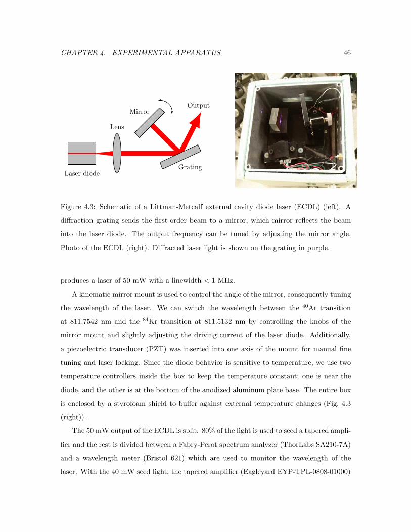
CHAPTER 4. EXPERIMENTAL APPARATUS 46
Laser diode
Lens
Mirror
Grating
Output
Figure 4.3: Schematic of a Littman-Metcalf external cavity diode laser (ECDL) (left). A
diffraction grating sends the first-order beam to a mirror, which mirror reflects the beam
into the laser diode. The output frequency can be tuned by adjusting the mirror angle.
Photo of the ECDL (right). Diffracted laser light is shown on the grating in purple.
produces a laser of 50 mW with a linewidth < 1 MHz.
A kinematic mirror mount is used to control the angle of the mirror, consequently tuning
the wavelength of the laser. We can switch the wavelength between the 40Ar transition
at 811.7542 nm and the 84Kr transition at 811.5132 nm by controlling the knobs of the
mirror mount and slightly adjusting the driving current of the laser diode. Additionally,
a piezoelectric transducer (PZT) was inserted into one axis of the mount for manual fine
tuning and laser locking. Since the diode behavior is sensitive to temperature, we use two
temperature controllers inside the box to keep the temperature constant; one is near the
diode, and the other is at the bottom of the anodized aluminum plate base. The entire box
is enclosed by a styrofoam shield to buffer against external temperature changes (Fig. 4.3
(right)).
The 50 mW output of the ECDL is split: 80% of the light is used to seed a tapered ampli-
fier and the rest is divided between a Fabry-Perot spectrum analyzer (ThorLabs SA210-7A)
and a wavelength meter (Bristol 621) which are used to monitor the wavelength of the
laser. With the 40 mW seed light, the tapered amplifier (Eagleyard EYP-TPL-0808-01000)

CHAPTER 4. EXPERIMENTAL APPARATUS 47
Figure 4.4: Schematic of the laser system.
produces 1.1 W of light that follows the characteristics of the seed light. Two isolators
(Conoptics 700) after the ECDL and the tapered amplifier prevent any reflected laser from
going backward into the diode. After the beam is properly shaped with lenses, the light is
sent through a single-mode polarization maintaining (PM) fiber. This is done to selectively
transfer the lowest-order laser mode and decouple any alignment drifts before the fiber
from the rest of the experiment. These optical components are set up on a damped optical
breadboard to isolate them from any vibrations of the table. The fiber ultimately provides
an output of around 550 mW to the cooling and trapping parts of the experiment.
After the fiber, 20 mW of the laser is split off and sent to a laser locking setup. The
light beams for transverse cooling, longitudinal slowing, trapping, and detecting atoms have
different powers and detunings from the atomic resonance, as detailed in Tab. 4.1. In order
to set the required detunings, the light from the PM fiber is passed through three acousto-
optic modulators (AOM). Each AOM acts as a transmission grating: the zeroth order beam
has zero frequency shift and the higher order beams have frequency shifts that depend on
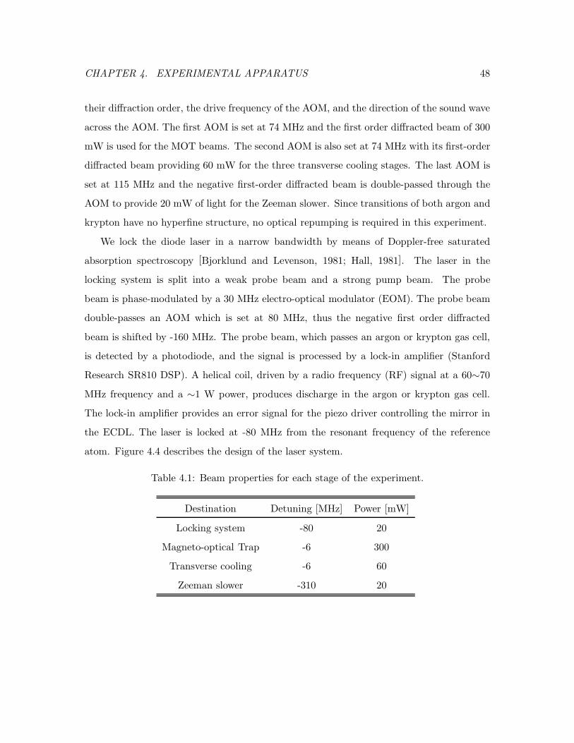
CHAPTER 4. EXPERIMENTAL APPARATUS 48
their diffraction order, the drive frequency of the AOM, and the direction of the sound wave
across the AOM. The first AOM is set at 74 MHz and the first order diffracted beam of 300
mW is used for the MOT beams. The second AOM is also set at 74 MHz with its first-order
diffracted beam providing 60 mW for the three transverse cooling stages. The last AOM is
set at 115 MHz and the negative first-order diffracted beam is double-passed through the
AOM to provide 20 mW of light for the Zeeman slower. Since transitions of both argon and
krypton have no hyperfine structure, no optical repumping is required in this experiment.
We lock the diode laser in a narrow bandwidth by means of Doppler-free saturated
absorption spectroscopy [Bjorklund and Levenson, 1981; Hall, 1981]. The laser in the
locking system is split into a weak probe beam and a strong pump beam. The probe
beam is phase-modulated by a 30 MHz electro-optical modulator (EOM). The probe beam
double-passes an AOM which is set at 80 MHz, thus the negative first order diffracted
beam is shifted by -160 MHz. The probe beam, which passes an argon or krypton gas cell,
is detected by a photodiode, and the signal is processed by a lock-in amplifier (Stanford
Research SR810 DSP). A helical coil, driven by a radio frequency (RF) signal at a 60∼70
MHz frequency and a ∼1 W power, produces discharge in the argon or krypton gas cell.
The lock-in amplifier provides an error signal for the piezo driver controlling the mirror in
the ECDL. The laser is locked at -80 MHz from the resonant frequency of the reference
atom. Figure 4.4 describes the design of the laser system.
Table 4.1: Beam properties for each stage of the experiment.
Destination Detuning [MHz] Power [mW]
Locking system -80 20
Magneto-optical Trap -6 300
Transverse cooling -6 60
Zeeman slower -310 20

CHAPTER 4. EXPERIMENTAL APPARATUS 49
4.2 Vacuum system
The system is maintained at ultra-high vacuum to prevent the metastable atoms from scat-
tering off background atoms. The vacuum system is composed of the following components:
a sample reservoir, a source chamber, three transverse cooling chambers, and a magneto-
optical trap chamber. Each stage is differentially pumped down so that the source chamber
has a higher pressure and the MOT chamber has a relatively low pressure. A schematic of
the vacuum system in shown in Fig. 4.5.
Argon, xenon, and krypton bottles are connected to the reservoir via regulators. The
reservoir is pumped down by a turbopump system (Pfeiffer Vacuum TSU 071 E, pumping
speed 59 l/s for nitrogen) including a dry diaphragm pump when the system is not in
operation. A valve to the pump is closed when the reservoir is filled with gas for operation.
We fine-control the gas flow from the reservoir to the system using a stainless steel ultra-fine
leak valve (Lesker VZLVM267) installed between the reservoir and the source chamber. The
source chamber is connected to the first TC chamber via a custom made copper gasket with
a 0.25” hole for the purpose of differential pumping. A turbopump (Pfeiffer Vacuum TMU
262 P, pumping speed 210 l/s for nitrogen) pumps down the first transverse cooling chamber
and the source chamber. The first and second transverse cooling chambers are separated
by a gate valve, which is open only when the system is running. A turbopump (Pfeiffer
Vacuum HiPace 80, pumping speed 67 l/s for nitrogen) is used to pump down the second
transverse cooling chamber. A differential pumping tube with a radius 0.32 cm connects the
second transverse cooling chamber and the Zeeman slower. Another turbopump (Pfeiffer
Vacuum TMU 262 P) is used to maintain vacuum in the MOT chamber. These three
turbopumps are backed by a main pump station which has a turbopump and a diaphragm
pump. Pneumatic valves are on the outputs of the three turbopumps so that we can break
the vacuum to the backing pump station while maintaining vacuum in the system. A failsafe
circuit was built to close the valves automatically in the case of a power failure.
To monitor the pressure, we use combined Pirani/cold-cathode gauges (PIG) (Pfeiffer
Vacuum PKR 251, PKR 261, and KIR 270) at each stage. Additionally, a pressure trans-
ducer (Stellar Technology GT1600-25A0331) with a quoted accuracy of 0.1% is used to
detect a high pressure in the reservoir, and a capacitive manometer (Pfeiffer Vacuum CMR

CHAPTER 4. EXPERIMENTAL APPARATUS 50
Figure 4.5: Schematic of the vacuum system. The vacuum is monitored by a pressure
transducer (D), capacitive manometer (C), combined Pirani/cold cathode gauges (PIG),
and a residual gas analyzer (RGA)
365) with a quoted accuracy of 0.5% was attached in the source chamber for the precise
pressure measurement, which is necessary to keep the consumption rate constant. A residual
gas analyzer (RGA) (Extorr Inc. XT200) also monitors the pressure in the MOT chamber
via mass spectrometry. When the system is not in operation, the vacuum is maintained at
∼ 10−7 torr in the source chamber, low 10−8 torr in the second transverse cooling chamber,
and low 10−9 torr in the MOT chamber. The gas flow is monitored and controlled via the
pressure in the source chamber, which is usually in the range of 0.01 ∼ 0.1 mtorr.
4.3 RF discharge source
4.3.1 Possible excitation methods
Because of the absence of lasers with sufficiently short wavelengths resonant with tran-
sitions from the ground state of krypton, we use a transition from the metastable state
5s[3/2]2 (3P2) to 5p[5/2]3 (3D3) for trapping and detecting. For this purpose, we first need
to excite ground state atoms to the metastable state, with the energy of 9.9 eV above the
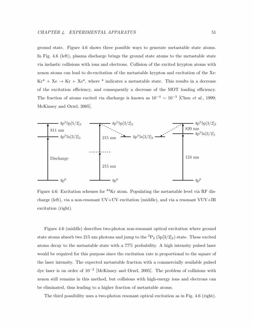
CHAPTER 4. EXPERIMENTAL APPARATUS 51
ground state. Figure 4.6 shows three possible ways to generate metastable state atoms.
In Fig. 4.6 (left), plasma discharge brings the ground state atoms to the metastable state
via inelastic collisions with ions and electrons. Collision of the excited krypton atoms with
xenon atoms can lead to de-excitation of the metastable krypton and excitation of the Xe:
Kr* + Xe → Kr + Xe*, where * indicates a metastable state. This results in a decrease
of the excitation efficiency, and consequently a decrease of the MOT loading efficiency.
The fraction of atoms excited via discharge is known as 10−4 ∼ 10−3 [Chen et al., 1999;
McKinsey and Orzel, 2005].
4p6
4p55s[3/2]2
4p55p[5/2]3
Discharge
811 nm
4p6
4p55p[3/2]2
215 nm
215 nm 4p55s[3/2]2
4p6
4p55p[3/2]2
4p55s[3/2]1
820 nm
124 nm
Figure 4.6: Excitation schemes for 84Kr atom. Populating the metastable level via RF dis-
charge (left), via a non-resonant UV+UV excitation (middle), and via a resonant VUV+IR
excitation (right).
Figure 4.6 (middle) describes two-photon non-resonant optical excitation where ground
state atoms absorb two 215 nm photons and jump to the 3P2 (5p[3/2]2) state. These excited
atoms decay to the metastable state with a 77% probability. A high intensity pulsed laser
would be required for this purpose since the excitation rate is proportional to the square of
the laser intensity. The expected metastable fraction with a commercially available pulsed
dye laser is on order of 10−2 [McKinsey and Orzel, 2005]. The problem of collisions with
xenon still remains in this method, but collisions with high-energy ions and electrons can
be eliminated, thus leading to a higher fraction of metastable atoms.
The third possibility uses a two-photon resonant optical excitation as in Fig. 4.6 (right).

CHAPTER 4. EXPERIMENTAL APPARATUS 52
A 124 nm laser excites ground state atoms to the 5s[3/2]1 state, then a 820 nm laser is used
to bring up these atoms to the 5p[3/2]2 state. Atoms in this state decay to the metastable
state with a 77% probability as discussed in the previous paragraph. While the resonant
interaction in this scheme allows a high efficiency (on order of ∼ 10−2) [Young et al., 2002],
this system requires two additional wavelengths and increases complexity.
4.3.2 RF discharge resonator
Figure 4.7: Cross section of the RF discharge source. The gas expands through an AlN
tube which is cooled by a cold finger. A plasma is generated by an RF signal applied to the
copper coil, producing metastable atoms. Temperature is monitored by a Pt100 platinum
resistive temperature sensor.
In this experiment, we use the discharge method to produce metastable atoms. A helical
resonator creates discharge, where the design parameters are based on Refs. [Macalpine and
Schildknecht, 1959; Chen et al., 2001]. The schematic is shown in Fig. 4.7. The resonator
consists of a helical coil and a brass shield; 18 American wire gauge (AWG) bare copper
wire was used in making the coil. The coil has a length of 7.6 cm and an inner diameter
of 3.4 cm, containing 16 windings. One end of the coil is connected to the shield, which is
11.1 cm long with an inner diameter of 6.34 cm, and the other end is connected to the RF

CHAPTER 4. EXPERIMENTAL APPARATUS 53
power wire. A Macor ceramic spacer supports the coil, and prevents it from sagging due to
gravity.
During operation, the source is cooled by a pulse tube refrigerator (Iwatani PDC08)
to reduce the atomic velocity, which results in a higher capture fraction by the Zeeman
slower. The atoms flow through an aluminium nitride (AlN) tube inside the resonator coil.
The thermally conductive and electrically insulating property of AlN allows efficient cooling
without an effect on plasma discharge. A platinum resistive thermometer Pt100 reads the
temperature at the end of the tube. There is a viewport on the back side of the source for
observing the discharge status. Figure 4.8 shows the picture of the assembled source.
Figure 4.8: Image of the helical coil RF resonator.
A voltage controlled oscillator generates the RF signal to the resonator. A small amount
of this power is split off and used for signal monitoring by a spectrum analyzer (Hameg
Instruments HMS1000), and the main part of the signal is amplified by an RF amplifier
(Mini-Circuits ZHL-50W-52-S). A SubMiniature version A (SMA) cable transfers the output
signal of the amplifier into the source. The impedances of the amplifier and the source needs
to be matched carefully for the best performance of the source [Sukenik and Busch, 2002].

CHAPTER 4. EXPERIMENTAL APPARATUS 54
When switching on the plasma source, we increase the RF power until the source lights,
then reduce the power to find the best system efficiency, as the source has a hysteresis
property. As long as the efficiency remains stable, the minimal power is preferred to re-
duce heating, subsequently reducing the atomic velocity. The performance of the source
depends on many parameters: frequency and power of the RF signal, source pressure, and
temperature inside the chamber. We empirically find the optimal parameters maximizing
the excitation efficiency, which is monitored via the MOT intensity. The typical operating
parameters are ∼15 W of applied RF power at ∼115 MHz, at a pressure of ∼0.1 mtorr
and temperature of ∼160 K. The discharge colors of argon gas and xenon gas are shown in
Fig. 4.9.
Figure 4.9: Glowing plasma discharge of argon gas (left) and xenon gas (right) by a helical
coil resonator.
4.4 Transverse cooling of the atomic beam
Three transverse cooling stages in the ATTA system collimate the atomic beam using optical
molasses with 6 MHz red detuned lasers. These stages significantly enhance the loading
rate of the MOT.

CHAPTER 4. EXPERIMENTAL APPARATUS 55
The first transverse cooling chamber has four windows of a 9.5 cm diameter in 6” flanges.
Since the argon beam has the most probable velocity of ∼300 m/s, and the krypton beam
∼200 m/s at the operating temperature, the atoms pass the interaction region quickly.
The longer the interaction between atom and light, the higher the collimation efficiency.
Therefore we extend the interaction region by reflecting the laser multiple times between
two flat mirrors as Fig. 4.10 (left) shows. This allows the longer interaction times, ans has
an advantage of a high laser intensity compared to expanding the beam size with fewer
reflections. The laser beam is slightly focused to compensate for the decrease of laser power
due to absorption by atoms and losses at window surfaces. The interaction time with the
laser is 3× 10⁻⁴ s for the argon beam, and 5× 10⁻⁴ s for the krypton beam. This will allow
each argon atom to experience ∼ 2× 10³ scatters, and krypton atom ∼ 3× 10³ scatters at
the laser intensity of a few Isat.
Atomic
beam
-6 MHz red
shifted laser
Mirror
Mirror
Figure 4.10: Schematic (left) and photo (right) of the first transverse cooling setup. The
−6 MHz detuned laser is reflected multiple times between two mirrors and sets up optical
molasses.
Figure 4.10 (right) shows the setup of the first transverse cooling stage. Two fiber optic
cables deliver the light to the vertical and horizontal axes. Each light beam is expanded to a
1 cm diameter by a telescope, and has an intensity of ∼5 mW/cm2. This intensity balances
the efficiency and the amount of laser power used. The efficiency of the first transverse

CHAPTER 4. EXPERIMENTAL APPARATUS 56
cooling is shown in Fig. 4.11 as a function of the laser intensity. We adjust the laser beam
paths with the mirrors and fiber optic mounts to optimize the transverse cooling efficiency,
which is monitored via the MOT intensity.
Laser Intensity [mW/cm^2]0.5 1 1.5 2 2.5 3 3.5 4 4.5 5
Effi
cien
cy
0
1
2
3
4
5
6
The 1st TC efficiency versus laser intensity
Figure 4.11: First-stage transverse cooling efficiency as a function of the laser intensity,
measured with the horizontal beam only.
The atomic beam leaving the first transverse cooling chamber is further collimated by
the second transverse cooling stage. The output laser is first expanded to a 0.5 cm diameter
by a telescope, then extended along one axis by two convex cylindrical lenses, for a final
size of 0.5 cm × 3 cm and an intensity of 3 mW/cm2. The chamber has windows in 2.75”
flanges allowing the laser beam to pass through. A mirror on the other side of vacuum cross
reflects the laser perpendicularly so that the two beams counterpropagate. At first, this
stage was designed for a bow-tie configuration with only one laser beam, but later changed
to a retro-reflecting configuration with two beams due to difficulty in aligning.
The third transverse cooling stage was installed following the Zeeman slower since scat-
tering inside the slower makes the atomic beam disperse before reaching the MOT chamber.
As the longitudinal velocity of the atomic beam is reduced by the Zeeman slower, sufficient

CHAPTER 4. EXPERIMENTAL APPARATUS 57
interaction time can be achieved with a small size beam. Thus a 1.33” cube is used for the
third transverse cooling chamber. The output light from a fiber optic cable is expanded to
a 1 cm diameter at a 3 mW/cm2 intensity. Since the atoms are slowed to the final velocity
of 30 m/s, the atoms experience an interaction time with the light of 3 × 10⁻⁴ s, which is
similar to the case of the first transverse cooling.
4.5 Zeeman atom slower
4.5.1 Design
In the Zeeman slower, a spatially tuned magnetic field B along the atomic beam keeps
a red-detuned slowing laser beam always near resonance. In this subsection, we find the
optimal Zeeman slower design.
Deceleration from the light pressure force in a Zeeman slower is expressed as
a(v, z) =F (v, z)
m= − hkΓ
2m
s0(z)
1 + s0(z) +
(δ + kv(z) − µ′B(z)/h
Γ/2
)2. (4.1)
In the denominator, the relation of Eq. 3.26 was used. As introduced in Sec. 3.3, µ′ is the
effective magnetic moment of the transition, µ′ = µB(MeJ g
eJ −Mg
J ggJ ), where g and e refer
to ground and excited states [Metcalf and van der Straten, 1999]. The Lande g-factor is
given by
gJ = 1 +J(J + 1) + S(S + 1)− L(L+ 1)
2J(J + 1), (4.2)
such that gJ(3P2) = 3/2 and gJ (
3D3) = 4/3.
Possible transitions between 3P2 and 3D3 are described in Fig. 4.12 with energy levels
shifted by the Zeeman effect. The strength of a transition is given by the square of the
transition dipole moment,
µeg = e(−1)Le+S−MeJ
√(2Jg + 1)(2Je + 1)
×
Le Je Sg
Jg Lg 1
Jg 1 Je
MgJ q −M e
J
〈αeLe ||r||αgLg〉 , (4.3)
where q is the light polarization, and α represents all properties of the state besides its orbital
angular momentum. When it comes to the transition of our interest, 3P2 - 3D3, all terms
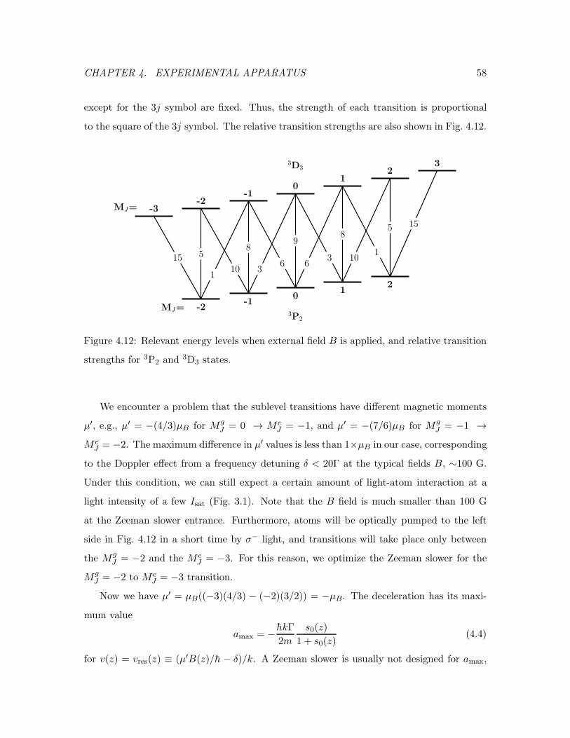
CHAPTER 4. EXPERIMENTAL APPARATUS 58
except for the 3j symbol are fixed. Thus, the strength of each transition is proportional
to the square of the 3j symbol. The relative transition strengths are also shown in Fig. 4.12.
58
98
5
15
110 3
6 63 10
1
15
MJ= -2-1
01
2
MJ= -3-2
-10
12
3
3P2
3D3
Figure 4.12: Relevant energy levels when external field B is applied, and relative transition
strengths for 3P2 and 3D3 states.
We encounter a problem that the sublevel transitions have different magnetic moments
µ′, e.g., µ′ = −(4/3)µB for MgJ = 0 → M e
J = −1, and µ′ = −(7/6)µB for MgJ = −1 →
M eJ = −2. The maximum difference in µ′ values is less than 1×µB in our case, corresponding
to the Doppler effect from a frequency detuning δ < 20Γ at the typical fields B, ∼100 G.
Under this condition, we can still expect a certain amount of light-atom interaction at a
light intensity of a few Isat (Fig. 3.1). Note that the B field is much smaller than 100 G
at the Zeeman slower entrance. Furthermore, atoms will be optically pumped to the left
side in Fig. 4.12 in a short time by σ− light, and transitions will take place only between
the MgJ = −2 and the M e
J = −3. For this reason, we optimize the Zeeman slower for the
MgJ = −2 to M e
J = −3 transition.
Now we have µ′ = µB((−3)(4/3) − (−2)(3/2)) = −µB. The deceleration has its maxi-
mum value
amax = − hkΓ2m
s0(z)
1 + s0(z)(4.4)
for v(z) = vres(z) ≡ (µ′B(z)/h − δ)/k. A Zeeman slower is usually not designed for amax,

CHAPTER 4. EXPERIMENTAL APPARATUS 59
since any imperfections will result in atoms that are too fast to decelerate. Instead, we
design for a(z) = ǫamax(z), with 0 < ǫ < 1. By inserting a(z) = ǫamax(z) into Eq. 4.1, we
derive the velocity trajectory
vǫ(z) = vres(z)−Γ
2k
√[1 + s0(z)]
1 − ǫ
ǫ. (4.5)
Now we need the optimal value of s0 and ǫ. The damping coefficient of the scattering
force α ≡ −∂F (v)/∂v ∝ s0/(1 + s0)2 is maximized at s0 = 1. The strength of the decel-
eration force F (v) ∝ s0/(1 + s0) monotonically increases 0 → 1 with increasing s0, and
reaches half-strength at s0 = 1. The product F (v)×∂F (v)/∂v is maximized at s0 = 2. The
cooling is proportional to ∂F (v)/∂v, and the best cooling is achieved if ∂2F (v)/∂v2 = 0.
This condition is satisfied when ǫ = 2s0/(1 + s0). When s0 = 2, ǫ = 0.75. To account for
experimental imperfections of the Zeeman slower, we design the Zeeman slower for ǫ = 0.65.
Figure 4.13: Design field for the Zeeman slower with a 310 MHz red detuned laser.
The final velocity is set to vf = 15 m/s, which should be well within the capture range
of the krypton and argon MOTs. An atom is then accelerated toward the Zeeman slower
entrance such that the backward velocity evolves as
dvb(z′)
dz′=ab(z
′)
v(z′), (4.6)

CHAPTER 4. EXPERIMENTAL APPARATUS 60
where the backward acceleration ab = ǫ|amax(Kr)| and z′ is the backward coordinate along
the Zeeman slower. The Kr parameters are used in the expression for ab(z′) because the
efficiency is most crucial for krypton. Inverting the coordinate z′ → z we obtain a velocity
trajectory, V (z). The design magnetic field B(z) is then
B(z) =h[δ0 + kvres(z)]
µ
=h
µ
(δ0 + kV (z) +
Γ
2
√[1 + s0(z)]
1 − ǫ
ǫ
). (4.7)
As shown in Fig. 4.13, the choice of δ0 = −310 MHz corresponds to all positive values of B
inside the Zeeman slower.
Finally, the v(z) trajectories for either krypton or argon are calculated starting from the
initial velocity v0, and applying the deceleration
a(z) = −0.65
0.75
hkΓ
2m
s0(z)
1 + s0(z) +
(δ0 + kv(z) − µB(z)/h
Γ/2
)2, (4.8)
where the prefactor of 0.65/0.75 ≈ 0.87 allows for the experimental imperfections of B(z).
The Zeeman slower length lZS = 75 cm is constrained by the table size, and the above
assumptions lead to the Zeeman slower capture velocities vc(Kr) ≈ 245 m/s, vc(Ar) ≈ 250
m/s. The velocity trajectories for argon and krypton beams are plotted in Fig. 4.14.
Based on the geometry of the vacuum system, the MOT is 15 cm from the optical
window for the Zeeman slower light, and a 75 cm Zeeman slower region begins another 25
cm further. Over this 1.15 m span, we focus the light so that it decreases from a ∼1.2 cm
diameter at the window to a ∼0.6 cm diameter at the Zeeman slower differential pumping
tube exit. This provides a small amount of transverse cooling, and compensates for the light
power decrease through absorption. Roughly, this gives a ∼1 cm diameter light beam at the
Zeeman slower exit. Given s0 = 1.5 and Isat = 1.4 mW/cm2, the Zeeman slower requires
an optical power of only ∼2 mW. A telescope with one concave lens and one convex lens is
carefully aligned so that the light beam is expanded to an appropriate diameter (> 1.2 cm)
and focused gently as designed above.
For a temperature T (in Kelvin), the thermal velocity for each species is v ≡√kBT/m.
The fraction of the atoms with a velocity v below the Zeeman slower capture velocity vc is

CHAPTER 4. EXPERIMENTAL APPARATUS 61
Figure 4.14: Velocity trajectories of argon (top) and krypton (bottom) in the Zeeman slower.
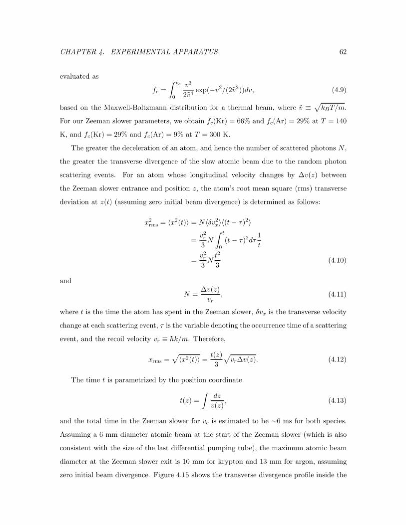
CHAPTER 4. EXPERIMENTAL APPARATUS 62
evaluated as
fc =
∫ vc
0
v3
2v4exp(−v2/(2v2))dv, (4.9)
based on the Maxwell-Boltzmann distribution for a thermal beam, where v ≡√kBT/m.
For our Zeeman slower parameters, we obtain fc(Kr) = 66% and fc(Ar) = 29% at T = 140
K, and fc(Kr) = 29% and fc(Ar) = 9% at T = 300 K.
The greater the deceleration of an atom, and hence the number of scattered photons N ,
the greater the transverse divergence of the slow atomic beam due to the random photon
scattering events. For an atom whose longitudinal velocity changes by ∆v(z) between
the Zeeman slower entrance and position z, the atom’s root mean square (rms) transverse
deviation at z(t) (assuming zero initial beam divergence) is determined as follows:
x2rms = 〈x2(t)〉 = N〈δv2x〉〈(t− τ)2〉
=v2r3N
∫ t
0
(t− τ)2dτ1
t
=v2r3Nt2
3(4.10)
and
N =∆v(z)
vr, (4.11)
where t is the time the atom has spent in the Zeeman slower, δvx is the transverse velocity
change at each scattering event, τ is the variable denoting the occurrence time of a scattering
event, and the recoil velocity vr ≡ hk/m. Therefore,
xrms =√
〈x2(t)〉 = t(z)
3
√vr∆v(z). (4.12)
The time t is parametrized by the position coordinate
t(z) =
∫dz
v(z), (4.13)
and the total time in the Zeeman slower for vc is estimated to be ∼6 ms for both species.
Assuming a 6 mm diameter atomic beam at the start of the Zeeman slower (which is also
consistent with the size of the last differential pumping tube), the maximum atomic beam
diameter at the Zeeman slower exit is 10 mm for krypton and 13 mm for argon, assuming
zero initial beam divergence. Figure 4.15 shows the transverse divergence profile inside the

CHAPTER 4. EXPERIMENTAL APPARATUS 63
Zeeman slower.
Figure 4.15: Transverse divergence for the highest captured velocity groups of krypton (245
m/s) and argon (250 m/s). The maximum divergence appears to be ∼2.2 mm radius over
the 75 cm Zeeman slower length for krypton and ∼3.4 mm for argon. The atomic beam
is expected to continue expanding on the way to the MOT, in the absence of transverse
cooling.
After the Zeeman slower, the beam will continue to expand as it travels ∼24 cm to the
MOT. The beam must clear the 1.5 cm inner diameter of the Zeeman slower tube, and
ideally be < 2 cm diameter by the time it reaches the MOT. For vc, the transverse velocity
at the Zeeman slower exit is given by
v2x, rms = 〈v2x〉 = N〈δv2x〉 =Nv2r3, (4.14)
vx, rms = vr
√N
3=
√∆vzvr
3, (4.15)
where vx, rms is ∼0.67 m/s for krypton and ∼0.98 m/s for argon. Thus, assuming a 15 m/s
slowed atom velocity and a 24 cm free propagation length, we obtain the total atom beam

CHAPTER 4. EXPERIMENTAL APPARATUS 64
diameters at the MOT of 3.2 cm for krypton and 4.5 cm for argon. The third transverse
cooling after the Zeeman slower is needed to compensate for this expansion.
4.5.2 Construction
We built the Zeeman slower in the traditional tapered solenoid design. The coil was designed
to have 18 longitudinal sections, and each section has one more layer of winding than the
previous section, e.g. the first section has one layer and the second section has two layers.
An exception is that the last section has 14 layers more than the previous one to produce
the sharp peak of the B field at the end of the Zeeman slower as shown in Fig. 4.13. Each
layer consists of a single, continuous 18 AWG kapton encapsulated copper wire starting at
a copper plate, and ending at a particular length, depending on the section number. A
square copper tube was welded on the plate to remove the dissipated heat.
Figure 4.16: A copper plate on which a square copper tube was welded for water cooling
(left). Zeeman slower winding on a lathe (right).
An aluminum pipe with a 1.5” outer diameter was used as a frame. We used a lathe for
winding and secured the first and last ∼1.5” of each layer with Loctite five min epoxy. After
a layer was wound and epoxied at both ends, we applied two coats of electrically insulating
varnish (Lakeshore VGE-7031). The first coat was allowed to dry before the second was
applied. This serves the dual purpose of insulating and minimizing the indentations between
the wires. The actual length of the Zeeman slower is 77.6 cm, which generates the desired

CHAPTER 4. EXPERIMENTAL APPARATUS 65
B field trajectory of 75 cm. The total length of the wire is ∼1975 m, and its weight is ∼15
kg.
The field profile from the Zeeman slower geometry is expressed as
B(z) =µ0NI
2
18∑
j=1
z − zij√
r2j + (z − zij )2−
z − zfj√r2j + (z − zfj )
2
, (4.16)
where zij and zfj are the coordinates of the beginning and end of the jth layer respectively,
I is the current, N is the winding number per unit length, and rj is the radius of the jth
layer. This field is shown with a green line in Fig. 4.17.
4.5.3 Field measurements
After the Zeeman slower was built, we measured the axial magnetic field using a custom
made gaussmeter which is based on the A1301 chip. An Ametek DLM 600 150-4 regulated
power supply provided current to the Zeeman slower. The gaussmeter was positioned in
the center of a nylon rod, which was held coaxially with the tube (to within ∼1mm) by a
teflon spacer. A motor driven piston (Firgelli Automation FA-400-L-12-24) pushed the rod
through the tube at a nearly constant rate while the gaussmeter was measuring the field.
The output from the gaussmeter was digitized by a National Instruments Data Acquisition
(DAQ) card. Data acquisition was started/stopped when the motor was started/stopped.
Thus we obtained the B field as a function of position. As the piston’s range is 61 cm, we
swept from one end and from the other end separately and merged the two in order to cover
the full range.
The first field measurement showed that the peak on the side of the copper plate was
not as sharp as the simulated field. We modified the coil by disconnecting the last section
and adding narrower layers of wire onto the outer layer. Since the radii of the new layers
are quite large (due to the thickness of the inner layers), a higher current is required than
what is needed for the rest of the slower. For this reason, we used a separate power supply
for the new outer layer to find the optimal current setting. The currents from the two
supplies were adjusted carefully to match the simulated B field. The currents of 0.67 A for
the inner coil and 2.73 A for the outer coil yield the best agreement with the simulation

CHAPTER 4. EXPERIMENTAL APPARATUS 66
Position [cm]0 20 40 60 80 100
B F
ield
[G]
0
20
40
60
80
100
120
140
160
180
200
Figure 4.17: Measurement of the Zeeman slower field in the longitudinal direction. The di-
rection of the atomic beam is defined as positive. The solid red line shows the ideal magnetic
field; the dashed green line shows the calculated magnetic field from the Zeeman slower de-
sign; black dots show the measured magnetic field. The fluctuations of the measured fields
are due to the internal fluctuations of the gaussmeter.

CHAPTER 4. EXPERIMENTAL APPARATUS 67
Figure 4.18: Velocity trajectory of Kr evaluated based on the measured Zeeman slower field.
(Fig. 4.17). The velocity trajectory for a krypton atom is simulated based on this measured
B field along the Zeeman slower (Fig. 4.18).
Once the optimized current values were found, a potentiometer was connected to dis-
tribute a current from a single power supply into the inner and outer layers with the above
fixed ratio for permanent use. Specifications for operating the Zeeman slower are summa-
rized in Tab. 4.2.
Table 4.2: Zeeman slower specifications.
Inner coil Outer coil Total
Length of wire [m] ∼1200 ∼360 ∼1560
Resistance [Ω] 2.97 0.88 3.85
Voltage across coil [V] 1.96 2.40
Current [A] 0.66 2.73
Heat dissipated [W] 1.27 8.88 10.2

CHAPTER 4. EXPERIMENTAL APPARATUS 68
4.6 Magneto-optical trap
A pair of anti-Helmholtz coils produce magnetic fields for three dimensional MOT as dis-
cussed in Sec. 3.4. The design of the coil was based on generating a magnetic field gradient
of 10 G/cm in the vertical (z) direction with a 30 A current. These numbers are confirmed
from the trajectories simulated for argon and krypton atoms in a one-dimensional MOT
(Fig. 4.19), that are derived from Eq. 3.4. For a laser diameter of 4 cm, the capture velocity
for argon is 35 m/s, and for krypton is 30 m/s. This indicates that the longitudinally de-
celerated atoms from the Zeeman slower, with a velocity of 15 m/s, are properly captured
by our MOT.
Figure 4.19: Atom trajectories in the one dimensional magneto-optical trap (MOT) for Ar
(left) and Kr (right). The simulation uses Parameters s0 = 5, δ/γ = −1, and dB/dz = 11
G/cm.
Both top and bottom MOT coils have nine layers on aluminum cylinders, and each layer
has nine windings. The z-component of the generated magnetic field along the z-axis (the
axis of coil winding) is simulated by
Bz(z) =µ0I
2
8∑
i=0
8∑
j=0
(r0 + id)2
((r0 + id)2 + (z − (z0 + jd))2)1.5− (r0 + id)2
((r0 + id)2 + (z + (z0 + jd))2)1.5,
(4.17)
where µ0 is the vacuum permeability, I is the current, r0 is the radius of the cylinder, d is
the thickness of the coil, z is the distance referenced to the center of the MOT, and i, j

CHAPTER 4. EXPERIMENTAL APPARATUS 69
indicate ith winding of the jth layer. The plots of this B field and its derivative are shown
in Fig. 4.21.
Figure 4.20: Winding the magneto-optical trap (MOT) coil (left) and MOT field measure-
ment (right).
We built the MOT coils using copper wire from S&W Wire. It has a circular hollow
inside a square cross section conductor to allow water to flow through the conductor and
remove the dissipated heat from the coil. Its kapton taped surface insulates the conductor.
We used the same lathe as for the Zeeman slower to wind the MOT coil, and varnished each
layer to ensure insulation (Fig. 4.20 (left)). Care must be taken to protect the insulated
surface from scratching during winding, since the wire is thick and stiff compared to the
wire of the Zeeman slower. After winding, JB Weld was applied on the outer layer to secure
the coil.
The MOT coils were brought to an optical table after construction, and set in the de-
signed geometry without the vacuum chamber for the magnetic field measurement. Due to
the complexity of the geometry, we manually positioned the gaussmeter instead of using
the motor driven piston (Fig. 4.20 (right)). The measured B field in the z-direction and

CHAPTER 4. EXPERIMENTAL APPARATUS 70
its derivative at the current of 30 A are shown in Fig. 4.21. As simulated, the coils have
its maximum B field of ∼120 G,and the dB/dz value at the MOT center is ∼11 G/cm.
Figure 4.22 shows the measured B field and its derivative along the x-axis, which is per-
pendicular to the z axis and the Zeeman slower axis. The magnitudes along the x-axis are
about half of those in the z axis, as predicted from geometry.
Position [cm]-20 -10 0 10 20
B F
ield
[G]
-100
-50
0
50
100
Position [cm]-20 -10 0 10 20
dB/d
z [G
/cm
]
-10
-5
0
5
10
Figure 4.21: Magneto-optical trap (MOT) field (top) and its derivative (bottom) in the
z-direction. Blue line is the simulation from the coil geometry, crosses are the measured
values, and red line is a fit to a high order polynomial equation.
We used Solidworks to design the chamber suitable for both trapping and detecting, and
it was custom-built by Kimball Physics. The chamber has four 4.5” flanges for detection,
six 2.75” flanges for trapping lasers, and two 1.33” flanges for the Zeeman slower window
and the connection to the vacuum system. We applied a low-outgassing black paint (AZ
Technologies MLS-85SB) to the inner surface of the chamber to avoid light reflections. Thus,
the surface is required to adhere the paint well. To choose the surface type, we tested the
paint with three samples of different surface finishes from Kimball physics. The finishes are
rough (Black Beauty sand, of unknown size), medium (blasted with #10 glass powder), and

CHAPTER 4. EXPERIMENTAL APPARATUS 71
Position [cm]-10 -5 0 5 10
B F
ield
[G]
-40
-20
0
20
40
Position [cm]-10 -5 0 5 10
dB/d
z [G
/cm
]
-8-7-6-5-4-3-2-10
Figure 4.22: Magneto-optical trap (MOT) field (top) and its derivative (bottom) in the x-
direction. Crosses are the measured values, and red line is a fit to a high order polynomial
equation.

CHAPTER 4. EXPERIMENTAL APPARATUS 72
highly polished. The paint adheres better to rougher surfaces, but still adheres reasonably
well to the highly polished finish. No flaking is observed, regardless of application thickness.
The highly polished finish was selected to avoid the possibility that gas is trapped between
the paint and the rough surface layer. We painted the chamber in a clean room at Columbia
University, which has a low level of environmental pollutants. However, it turned out that
the paint on the surface flakes off slightly after several weeks of operation.
As the windows should not be heated over 150C, we first baked the chamber closed
with blank flanges at a temperature ∼400C for a week, then the blank flanges were re-
placed with anti-reflection coated windows while nitrogen gas flushes the system to prevent
water and air from adhering to the walls during the process. After the windows installed,
the chamber was baked again at a lower temperature. An optical breadboard, which is 30
cm above the table, supports the MOT chamber and the optical components (Fig. 4.23).
One side of the breadboard was cut to avoid eddy currents induced by the MOT current
switching.
Figure 4.23: Chamber and coils for the Magneto-optical trap (MOT).
A power supply (Ametek DLM 600 150-4) provides the required current to the two
MOT coils connected in series. The hollow inside the wire is connected to a temperature
recirculating chiller (Thermo Scientific NESLAB Merlin M150) for water cooling. Addi-

CHAPTER 4. EXPERIMENTAL APPARATUS 73
tionally, three pairs of Helmholtz coils were added around the chamber to fine control the
zero point of the magnetic field, and consequently the position of the MOT, which is crit-
ical for alignment of the single atom detection system. Table 4.3 summarizes the MOT
specifications.
Table 4.3: Magneto-optical trap (MOT) specifications.
Top coil Bottom coil Total
Length of wire [m] ∼30 ∼30 ∼60
Resistance [Ω] 0.05 0.05 1.01
Voltage across coil [V] 1.48 1.48 2.98
Current [A] 27.9 27.9 27.9
Power dissipated [W] 41.4 41.4 82.8
The laser beam for the MOT is expanded to a 2 cm radius, and split into three beams
by beam splitting cubes. In our setup, the vertical beam has twice the power of horizontal
beams. As we discussed above, the polarization of each beam should be set for σ− transi-
tions, so λ/4 waveplates are used to adjust beam polarizations before and after the chamber
for each pair of beams. Three irises in front of the chamber adjust the sizes of the MOT
beams, which is useful in controlling background level for a good resolution of single atom
signals.
4.7 Laser shutter
Studies of the MOT loading and decaying are necessary for a detailed MOT characterization.
To obtain practical loading and decay plots, it is required to switch on and off the MOT
quickly so that the transition time does not affect the results. Switching the MOT can
be achieved by several methods: switching the MOT coil current, the trapping laser, the
Zeeman slower coil current, the Zeeman slower laser, or the atomic beam. Switching the
currents may introduce inductance problems, and switching the Zeeman slower involves a
possibility that residual slowed atoms in the system flow into the MOT after the Zeeman
slower is turned off. However, a very small fraction of atoms are still trapped even without

CHAPTER 4. EXPERIMENTAL APPARATUS 74
Figure 4.24: Custom-made laser shutter to mechanically switch on and off the Zeeman
slower laser. It is normally closed (left) without any driving signal, and is open (right)
while a 24 V input voltage is being applied.
the Zeeman slower. Blocking the atomic beam mechanically inside the vacuum would be
ideal since it eliminates the light scattered off the atomic beam in the trap chamber [Du,
2003], but this requires a relatively complex setup compared to other methods. We used a
mechanical shutter to block the Zeeman slower laser in this measurement.
The shutter consists of a solenoid relay (P&B Electronics T90N1D-12) that comes with a
small metal contact opposite an electromagnet. This contact was removed so the full beam
diameter could fit through the slot. Removing the contact increases the closing distance
between the two magnets, so the relay requires more voltage to function properly. A DAQ
card (National Instruments PCI Express 6321) and a terminal block (National Instruments
SCB-68) generate the driving signal of 5 V, which is converted to a 24 V signal by a custom-
made driver. The process is controlled with a C++ code using National Instrument DAQmx
library. Figure 4.25 shows the shutter when it is closed and open.
For testing, the shutter was placed in a laser path and a photodiode recorded the laser
power while the shutter switched on and off. The photodiode signal versus time is plotted in
Fig. 4.25, which shows that the opening delay is consistently longer than the closing delay.
The bounce in the optical signal can be avoided with careful alignment; if the light is too
near the closing stop, the bounce will be apparent. The shutter opens and closes sufficiently

CHAPTER 4. EXPERIMENTAL APPARATUS 75
Time [s]-0.2 -0.15 -0.1 -0.05 0 0.05 0.1 0.15 0.2 0.25
Pho
toio
de S
igna
l [V
]
0
1
2
3
4
5
6
7
8
9
10
Shutter Signals
Figure 4.25: Photodiode signal with time for opening (solid blue line) and closing (dashed
red line) of the shutter. The trigger signal is transmitted to the shutter at t = 0 for both
cases.
quickly that we did not see a marked effect from the transition.

CHAPTER 5. COOLING AND TRAPPING 76
Chapter 5
Cooling and trapping
One of the main challenges of this experiment is to achieve the loading rate that is high
enough to detect a part per trillion (ppt) level of krypton contamination within a reasonable
amount of time. A low loading rate would require a longer measurement time, which results
in stricter requirements on long-term system stability. We incorporated several stages to
increase the loading efficiency, and all the stages were adjusted and optimized carefully.
Argon gas was used for testing and optimization to avoid krypton contamination prior to
measuring xenon samples. This chapter deals the optimization processes for a high loading
efficiency, and characterizes in samples of trapped argon atoms.
5.1 Source cooling
As discussed in Sec. 4.5, the Zeeman slower can decelerate argon atoms with velocity below
250 m/s, and krypton atoms with velocity below 245 m/s. At equilibrium, particle velocity
distributions in gases can be described by the Maxwell-Boltzmann (MB) law, if atoms
or molecules have no internal structure and interact via other particles only via elastic
collisions. From the Boltzmann energy distribution, one can derive the one-dimensional
velocity distribution f(v),
f(v) =1√2πv
exp
(− v2
2v2
), (5.1)
where
v ≡√kBT
M. (5.2)
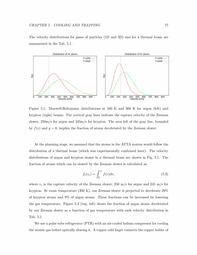
CHAPTER 5. COOLING AND TRAPPING 77
The velocity distributions for gases of particles (1D and 3D) and for a thermal beam are
summarized in the Tab. 5.1.
0 100 200 300 400 500 600 700 800 900
f(v)
Velocity [m/s]
Distribution of Ar atoms
T=160KT=300K
0 100 200 300 400 500 600 700 800 900
f(v)
Velocity [m/s]
Distribution of Kr atoms
T=160KT=300K
Figure 5.1: Maxwell-Boltzmann distributions at 160 K and 300 K for argon (left) and
krypton (right) beams. The vertical gray lines indicate the capture velocity of the Zeeman
slower, 250m/s for argon and 245m/s for krypton. The area left of the gray line, bounded
by f(v) and y = 0, implies the fraction of atoms decelerated by the Zeeman slower.
At the planning stage, we assumed that the atoms in the ATTA system would follow the
distribution of a thermal beam (which was experimentally confirmed later). The velocity
distributions of argon and krypton atoms in a thermal beam are shown in Fig. 5.1. The
fraction of atoms which can be slowed by the Zeeman slower is calculated as
fc(vc) =
∫ vc
0
f(v)dv, (5.3)
where vc is the capture velocity of the Zeeman slower; 250 m/s for argon and 245 m/s for
krypton. At room temperature (300 K), our Zeeman slower is projected to decelerate 29%
of krypton atoms and 9% of argon atoms. These fractions can be increased by lowering
the gas temperature. Figure 5.2 (top, left) shows the fraction of argon atoms decelerated
by our Zeeman slower as a function of gas temperature with each velocity distribution in
Tab. 5.1.
We use a pulse tube refrigerator (PTR) with an air-cooled helium compressor for cooling
the atomic gas before optically slowing it. A copper cold finger connects the copper holder of

CHAPTER 5. COOLING AND TRAPPING 78
Figure 5.2: Capture fraction of the Zeeman slower for 1D, 3D gases and for a beam of argon
atoms (top, left) and the relative intensity of magneto-optical trap (MOT) in the function
of temperature. Solid lines are the calculated capture fraction, and black dots are measured
MOT intensities, the data points are fitted to the distribution of 1D gas (top, right), 3D
gas (bottom, left), and beam (bottom, right). The data are independently scaled to the
level of each distribution curve.
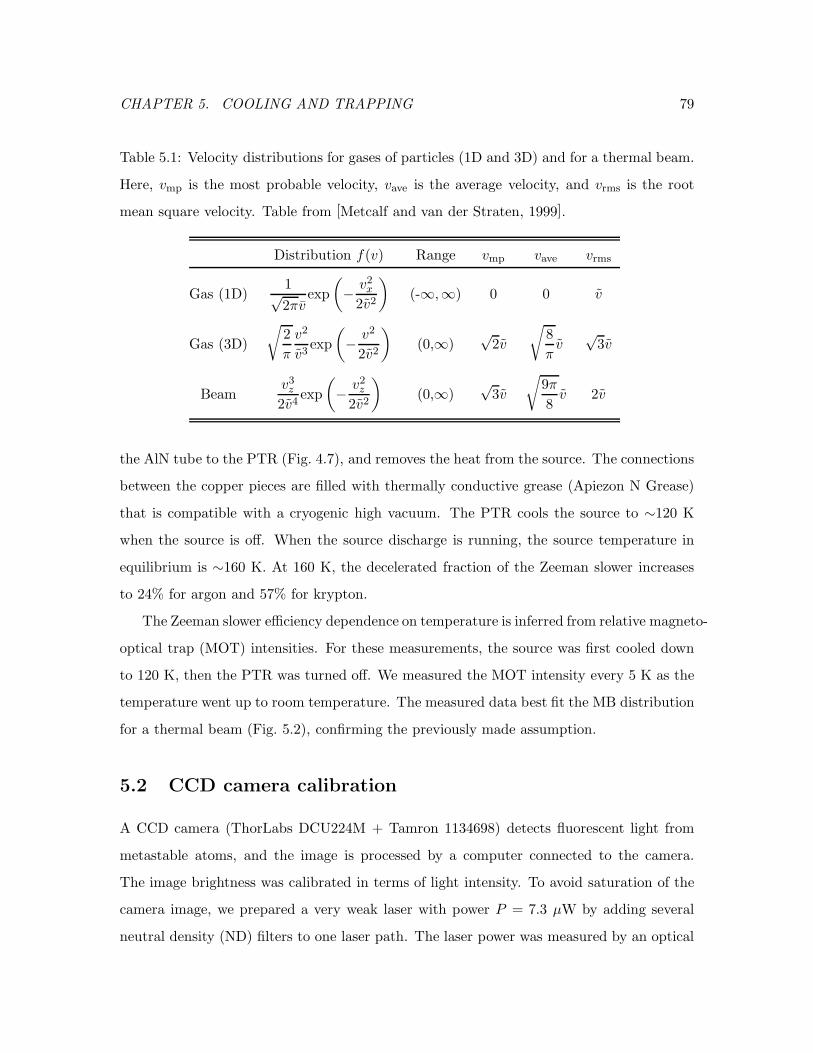
CHAPTER 5. COOLING AND TRAPPING 79
Table 5.1: Velocity distributions for gases of particles (1D and 3D) and for a thermal beam.
Here, vmp is the most probable velocity, vave is the average velocity, and vrms is the root
mean square velocity. Table from [Metcalf and van der Straten, 1999].
Distribution f(v) Range vmp vave vrms
Gas (1D)1√2πv
exp
(− v2x2v2
)(-∞,∞) 0 0 v
Gas (3D)
√2
π
v2
v3exp
(− v2
2v2
)(0,∞)
√2v
√8
πv
√3v
Beamv3z2v4
exp
(− v2z2v2
)(0,∞)
√3v
√9π
8v 2v
the AlN tube to the PTR (Fig. 4.7), and removes the heat from the source. The connections
between the copper pieces are filled with thermally conductive grease (Apiezon N Grease)
that is compatible with a cryogenic high vacuum. The PTR cools the source to ∼120 K
when the source is off. When the source discharge is running, the source temperature in
equilibrium is ∼160 K. At 160 K, the decelerated fraction of the Zeeman slower increases
to 24% for argon and 57% for krypton.
The Zeeman slower efficiency dependence on temperature is inferred from relative magneto-
optical trap (MOT) intensities. For these measurements, the source was first cooled down
to 120 K, then the PTR was turned off. We measured the MOT intensity every 5 K as the
temperature went up to room temperature. The measured data best fit the MB distribution
for a thermal beam (Fig. 5.2), confirming the previously made assumption.
5.2 CCD camera calibration
A CCD camera (ThorLabs DCU224M + Tamron 1134698) detects fluorescent light from
metastable atoms, and the image is processed by a computer connected to the camera.
The image brightness was calibrated in terms of light intensity. To avoid saturation of the
camera image, we prepared a very weak laser with power P = 7.3 µW by adding several
neutral density (ND) filters to one laser path. The laser power was measured by an optical
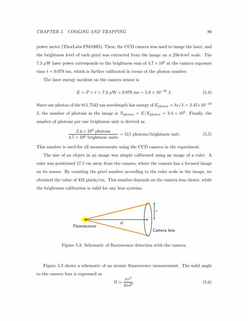
CHAPTER 5. COOLING AND TRAPPING 80
power meter (ThorLabs PM100D). Then, the CCD camera was used to image the laser, and
the brightness level of each pixel was extracted from the image on a 256-level scale. The
7.3 µW laser power corresponds to the brightness sum of 4.7× 10⁶ at the camera exposure
time t = 0.079 ms, which is further calibrated in terms of the photon number.
The laser energy incident on the camera sensor is
E = P × t = 7.3 µW× 0.079 ms = 5.8 × 10⁻¹⁰ J. (5.4)
Since one photon of the 811.7542 nm wavelength has energy of Ephoton = hc/λ = 2.45×10⁻¹⁹
J, the number of photons in the image is Nphoton = E/Ephoton = 2.4 × 10⁹. Finally, the
number of photons per one brightness unit is derived as
2.4× 10⁹ photons
4.7 × 10⁶ brightness units= 511 photons/brightness unit. (5.5)
This number is used for all measurements using the CCD camera in the experiment.
The size of an object in an image was simply calibrated using an image of a ruler. A
ruler was positioned 17.5 cm away from the camera, where the camera has a focused image
on its sensor. By counting the pixel number according to the ruler scale in the image, we
obtained the value of 432 pixels/cm. This number depends on the camera lens choice, while
the brightness calibration is valid for any lens systems.
Camera lens
d
r
Fluorescence
Figure 5.3: Schematic of fluorescence detection with the camera.
Figure 5.3 shows a schematic of an atomic fluorescence measurement. The solid angle
to the camera lens is expressed as
Ω ≃ πr2
4πd2, (5.6)

CHAPTER 5. COOLING AND TRAPPING 81
where r is the radius of the camera lens and d is the distance from the fluorescence source
to the camera lens. Using the value derived in Eq. 5.5 and camera parameters, we estimate
the number of atoms as
Natom = Brightness× 1
511× 1
Ω× 1
Rscatt× 1
texp× 1
G, (5.7)
where Rscatt is the scattering rate in Eq. 3.13 at the given light intensity and detuning, texp
is the exposure time, and G is the gain setting of the camera.
5.3 Consumption rate of argon
Figure 5.4: Pressure in the reservoir decreases linearly with time as the gas is consumed.
The pressure in the source chamber is maintained at 0.81 mtorr.
The gas consumption rate is defined as the number of atoms per second that come
into the system from the reservoir. To estimate the consumption rate of the source, we
filled the reservoir with argon gas and let it flow out into the source chamber through the
fine leak valve. The pressure in the reservoir was measured every two minutes (Fig. 5.4),
and the pressure change per unit time, dP (t)/dt, was derived. During the measurement,
the pressure at the source chamber was carefully maintained at a fixed level in order to
determine the consumption rate as a function of source pressure. The time derivative of
the ideal gas equation is (dP
dt
)V =
(dN
dt
)kBT, (5.8)

CHAPTER 5. COOLING AND TRAPPING 82
where V it the reservoir volume and N is the number of atoms. Then the consumption rate
is
C = −dN
dt=
dP
dt
V
kT. (5.9)
Table 5.2: Consumption rates of argon gas for different pressures in the source chamber.
Source chamber pressure [mtorr] 0.61 0.70 0.81 1.00
Consumption rate [1016 s−1] 5.8 6.5 7.8 9.2
The consumption rate was measured at several pressures in the source chamber around
0.8 mtorr, where the efficiency of the argon discharge is optimized. By inserting the esti-
mated reservoir volume V = 6.3× 10⁻⁴ m3 and the gas temperature T = 290 K, we obtain
consumption rates presented in Tab. 5.2, which are also plotted in Fig. 5.5.
Figure 5.5: Consumption rates of argon gas for different pressures in the source chamber.
The consumption rate increases linearly with the source chamber pressure. The gray region
shows 1 σ confidence interval.
5.4 Atomic flux
The study of the metastable atomic flux at the first transverse cooling stage together with
the consumption rate and the MOT loading rate characterizes the excitation efficiency of

CHAPTER 5. COOLING AND TRAPPING 83
the source and the cooling and trapping efficiency of the system. To measure the flux, a
fluorescence laser (~x) was set perpendicular to the atomic beam direction (~z), and the CCD
camera observed the fluorescence light from a horizontally transverse direction (~y). The
scheme of the measurement is shown in Fig. 5.6.
Figure 5.6: Schematic of the fluorescence measurement in the 1st transverse cooling (TC)
chamber.
Images were taken for several laser detunings, and the position and intensity of the
fluorescence light were analyzed in each image. The pressure in the source chamber was
maintained at 0.81 mtorr during the measurement. At various detunings, the laser interacts
with atoms that have corresponding velocities determined by the Doppler effect
f = f0 −∆f = (1− ∆v
c)f0, (5.10)
where f is the laser frequency. The fluorescence is located at x = 1.37 mm for the laser
locked to a detuning of ∆f = −5.61 MHz. With this detuning and Eq. 5.10, the transverse
velocity of the fluorescent atoms is derived as
vx = ∆v = c∆f
f0= 4.55 m/s. (5.11)
Since the horizontal distance z is much larger than the diameter of the AlN tube, we
assume that the atomic beam disperses from a single point (the end of the tube). Then we
have the relationvxx
=4.55 m/s
1.37 mm= 3.32 × 10³/s (5.12)

CHAPTER 5. COOLING AND TRAPPING 84
from the triangular geometry. Using this relation, the transverse atomic velocities at each
detuning atoms are derived in Tab. 5.3. It also allows us to estimate the longitudinal velocity
of the atomic beam,
vz = 85.3 mm× vxx
= 283 m/s. (5.13)
With the MB distribution of a thermal beam, the most probable velocity of 283 m/s leads
to the gas temperature of 129 K.
Table 5.3: Characteristics of fluorescent atoms at five different laser frequencies.
Position x [mm] Velocity vx [m/s] Relative intensity Atom density [106 mm−3]
0.45 1.5 100.0 5.83
5.25 17.5 72.0 4.20
9.30 31.0 42.8 2.50
12.15 40.5 29.7 1.73
14.85 49.5 21.3 1.24
The number of atoms in the fluorescence region is obtained from Eq. 5.7, then we
estimate the atom density n, using the laser beam size. The calculated atom densities are
presented in Tab. 5.3 and plotted in Fig. 5.7.
To estimate the atomic flux, the density n(x) has to be integrated over the cross sectional
area. By fitting a Gaussian distribution to the calculated atom densities, we determine the
atom density profile as a function of the distance from center,
f(x) = A exp
(− x2
2σ2
), (5.14)
where A = 5.4× 106 cm−3, and σ = 8.09 mm. Integrating Eq. 5.14 over the x-y plane gives
the linear density
nz =
∫∞
0
∫ 2π
0
f(x) dθ dx = 2πA σ2 = 2.22 × 107cm−1. (5.15)
Finally, the product of the longitudinal velocity (Eq. 5.13) and the linear density (Eq. 5.15)
determines the metastable atomic flux
Flux = vz × nz = 6.3× 10¹¹/s. (5.16)

CHAPTER 5. COOLING AND TRAPPING 85
Position [mm]-15 -10 -5 0 5 10 15
]-3
cm
6A
tom
ic d
ensi
ty [x
10
0
1
2
3
4
5
6
1st TC Fluorescence
Figure 5.7: Histogram of atomic densities as a function of position. The five data points at
positive values of x are measured, and are reflected through the origin for visualization.
Given the gas consumption rate at the 0.81 mtorr source chamber pressure (Tab. 5.2),
Eq. 5.16 yields the excitation efficiency of the discharge source of ∼ 10−5 for argon, which is
slightly lower than that in previous studies [Chen et al., 1999; McKinsey and Orzel, 2005].
5.5 Magneto-optical trap of argon
The argon MOT is observed by a CCD camera through a window in a 6” flange of the
MOT chamber. The camera is located 17.5 cm away from the center of the MOT chamber
on the optical table, resulting in a solid angle of 8.3 × 10⁻⁴ to the camera lens. From the
brightness sum of the MOT image, the number of trapped atoms is inferred using Eq. 5.7.
Since the frame speed of the CCD camera (30 frames/s) is not fast enough, a photodiode
(ThorLabs DET36A) is employed to read the MOT intensity through another window. The
output voltage from the photodiode is directly calibrated to the atom number derived from
the CCD camera.
For the maximum loading rate, all system parameters were carefully adjusted. During
optimization, the system efficiency was inferred via the number of trapped atoms which can

CHAPTER 5. COOLING AND TRAPPING 86
be observed in real time while deriving the loading rate requires additional measurements.
It turns out that the number of atoms is a good indicator of the loading rate in our case
(Eq. 5.18). Table 5.4 summarizes the contribution of each stage to signal enhancement. It
is more challenging to adjust the third transverse cooling stage than the first two because
the residual fields from the MOT and the Zeeman slower contribute unexpected Zeeman
shifts to the transition energy.
The Zeeman slower current was readjusted to find the brightest MOT from the current
previously determined by the field measurement, 0.67 A for the inner coil and 2.73 A for
the outer coil (Sec. 4.5.3). We obtained the new optimal currents of 0.66 A for the inner coil
and 3.17 A for the outer coil. The difference may be due to the residual field of the MOT
coil or the actual MOT capture velocity being different from the designed exit velocity of
the Zeeman slower (15 m/s). With the Zeeman slower off, we barely see any MOT image
from the CCD camera, but a small number of trapped atoms can be observed by single
atom detection.
Table 5.4: Contribution of each stage to the loading rate.
Stage Increase factor Notes
Source cooling 4
1st transverse cooling (TC) 20 4.5× 4.5
2nd TC 2
3rd TC 1.2
Zeeman slower >1000
The number of trapped atoms is modeled by
dN(t)
dt= L− N(t)
τ− βN(t)2, (5.17)
where L is the loading rate, τ is the mean trap lifetime, and β is the quadratic collision term.
The second term on the right-hand side represents the loss from collisions with background
atoms, and the third term indicates the loss from collisions between trapped atoms. If the
MOT volume expands with a fixed density when the number of trapped atoms increases,

CHAPTER 5. COOLING AND TRAPPING 87
Time [s]2.5 2.55 2.6 2.65 2.7 2.75
Num
ber
of a
tom
s
0
1
2
3
4
5
6
7
8
9610×
Loading measurement
Time [s]0.1 0.2 0.3 0.4 0.5 0.6 0.7
Num
ber
of a
tom
s
0
1
2
3
4
5
6
7
8
9
10610×
Number of trapped atoms
Figure 5.8: Loading (top) and decay (bottom) plots for the argon MOT. Black dots are
data, and red lines are fits to the solution of Eq. 5.18.

CHAPTER 5. COOLING AND TRAPPING 88
as is the case here, Eq. 5.17 is modified to
dN(t)
dt= L− N(t)
τ− βnN(t), (5.18)
where n is the fixed atom density [Steane et al., 1992; Marcassa et al., 1993]. Solving
Eq. 5.18 yields the solution
N(t) =L
1
τ+ βn
+ c1 exp
[−(1
τ+ βn
)t
], (5.19)
where c1 is a coefficient. Especially, when L = 0, the solution is
N(t) = N0
(1− exp
[−(1
τ+ βn
)t
]), (5.20)
where N0 is the equilibrium number of trapped atoms.
Table 5.5: Characteristics of the ATTA system with argon.
Parameters Values
Trapped atom number 8× 10⁶
Consumption rate 7.8× 10¹⁶ s−1
Metastable atom flux 6.3× 10¹¹ s−1
Source efficiency 0.8× 10⁻⁵
Loading rate 1.5× 10⁸ s−1
Overall efficiency 1.9× 10⁻⁹
Figure 5.8 shows the loading and decay plots for the argon MOT. Fitting Eq. 5.20 to
the decay data determines the values of the constant N0 and coefficients τ = 0.47 s and
βnc = 9.7/s. By inserting these into Eq. 5.18 in steady state, i.e., dN(t)/dt = 0, we obtain
the loading rate LAr = 1.79×10⁸/s. Taking into account the factor of 2.1 from the efficiency
enhancement of the Zeeman slower for krypton and assuming that other properties of the
system remain the same, we expect the krypton loading rate LKr = 3.76× 10⁸/s. Thus, the
loading rate for 1 ppt krypton contamination would be LKr−1ppt = 3.76× 10⁻⁴/s, implying
that it should take 78 minutes on average to load one trapped atom. The characteristics of
the argon MOT are summarized in Tab. 5.5.

CHAPTER 6. SINGLE ATOM DETECTION 89
Chapter 6
Single atom detection
It is essential to have the ability to detect single atom signals in order to measure trace
contaminations. The trapped atoms in the MOT are detected by the fluorescence light they
emit due to the MOT laser beams. In our MOT, one trapped argon atom emits ∼ 107
photons/s at sufficiently high laser intensities. To detect single atoms, we are required to
collect as many photons as possible with minimized background. The single atom detection
system was designed for this purpose. In this chapter, we discuss design and testing of this
system.
6.1 Avalanche photodiode
We use an avalanche photodiode (APD, Perkin-Elmer single photon counting module SPCM-
AQRH-12) to detect single atom signals. It has a quantum efficiency of 45% at 830 nm
and a dark count of 500 Hz according to the manufacturer’s specification. The measured
dark count in our lab is ∼300 s−1. The active area of the APD has a 180 µm diameter.
With a 50 Ω load, the APD generates a 2.5 V TTL pulse of a 15 ns width as each photon
is detected [Elmer, 2007].
As it is known that the single photon counting module (SPCM) can be damaged by
exposure to a 106 counts/s level of light for more than a few milliseconds [Gordon and
Selvin, 2003], we developed a failsafe circuit to protect the APD from overexposure using
a microcontroller (Arduino ATmega328). The schematic of the circuit is shown in Fig. 6.1.

CHAPTER 6. SINGLE ATOM DETECTION 90
Since the ATmega328 is not fast enough to count pulses at megahertz rates, the failsafe
circuit employs an external counter, 74LS590. The LS590 has an 8-bit binary counter that
feeds an 8-bit storage register, enabling the count value to be transferred to the register and
the counter cleared while the register is being read out. When the count rate exceeds 300
kHz, the circuit shuts off automatically and a red LED lights up. The failsafe also relays the
generated APD signal to a DAQ card (National Instruments PCI Express 6321) connected
to a computer. The signal is displayed and recorded in units of photons/s by a National
Instrument LabView program.
Figure 6.1: Prototype schematic of the APD failsafe circuit. Figure from [Gordon and
Selvin, 2003].
6.2 Optics
Figure 6.2 shows the sketch of our single atom detection system. The system was carefully
designed to efficiently gather the emitted photons from trapped atoms while filtering out any
background photons. The background comes from various sources: ambient light entering
through the chamber windows, fluorescence light from the atomic beam, and the MOT
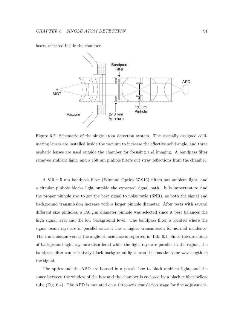
CHAPTER 6. SINGLE ATOM DETECTION 91
lasers reflected inside the chamber.
27.0 mm
Aperture
Bandpass
Filter
150 um
Pinhole
APD
MOT
Vacuum
Figure 6.2: Schematic of the single atom detection system. The specially designed colli-
mating lenses are installed inside the vacuum to increase the effective solid angle, and three
aspheric lenses are used outside the chamber for focusing and imaging. A bandpass filter
removes ambient light, and a 150 µm pinhole filters out stray reflections from the chamber.
A 810 ± 5 nm bandpass filter (Edmund Optics 67-916) filters out ambient light, and
a circular pinhole blocks light outside the expected signal path. It is important to find
the proper pinhole size to get the best signal to noise ratio (SNR), as both the signal and
background transmission increase with a larger pinhole diameter. After tests with several
different size pinholes, a 150 µm diameter pinhole was selected since it best balances the
high signal level and the low background level. The bandpass filter is located where the
signal beam rays are in parallel since it has a higher transmission for normal incidence.
The transmission versus the angle of incidence is reported in Tab. 6.1. Since the directions
of background light rays are disordered while the light rays are parallel in the region, the
bandpass filter can selectively block background light even if it has the same wavelength as
the signal.
The optics and the APD are housed in a plastic box to block ambient light, and the
space between the window of the box and the chamber is enclosed by a black rubber bellow
tube (Fig. 6.4). The APD is mounted on a three-axis translation stage for fine adjustment,
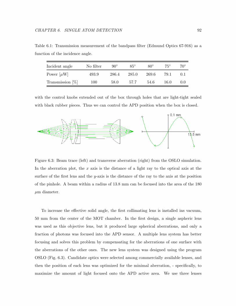
CHAPTER 6. SINGLE ATOM DETECTION 92
Table 6.1: Transmission measurement of the bandpass filter (Edmund Optics 67-916) as a
function of the incidence angle.
Incident angle No filter 90 85 80 75 70
Power [µW] 493.9 286.4 285.0 269.6 79.1 0.1
Transmission [%] 100 58.0 57.7 54.6 16.0 0.0
with the control knobs extended out of the box through holes that are light-tight sealed
with black rubber pieces. Thus we can control the APD position when the box is closed.
Figure 6.3: Beam trace (left) and transverse aberration (right) from the OSLO simulation.
In the aberration plot, the x axis is the distance of a light ray to the optical axis at the
surface of the first lens and the y-axis is the distance of the ray to the axis at the position
of the pinhole. A beam within a radius of 13.8 mm can be focused into the area of the 180
µm diameter.
To increase the effective solid angle, the first collimating lens is installed ins vacuum,
50 mm from the center of the MOT chamber. In the first design, a single aspheric lens
was used as this objective lens, but it produced large spherical aberrations, and only a
fraction of photons was focused into the APD sensor. A multiple lens system has better
focusing and solves this problem by compensating for the aberrations of one surface with
the aberrations of the other ones. The new lens system was designed using the program
OSLO (Fig. 6.3). Candidate optics were selected among commercially available lenses, and
then the position of each lens was optimized for the minimal aberration, - specifically, to
maximize the amount of light focused onto the APD active area. We use three lenses

CHAPTER 6. SINGLE ATOM DETECTION 93
instead of four, which is adopted in other groups [Alt, 2002; YanQiang et al., 2012], due
to the limited space inside the vacuum. The OSLO simulation shows that our system has
almost the same performance as a quadruple lens system. We expect that photons inside
the radius of 13.5 mm on the surface of the in-vacuum objective can be focused properly
by the optics. An aperture with a 13.5 mm diameter is mounted to block any light outside
this area since background is large than the signal in that region. This leads to the useful
solid angle of 1.8%.
Figure 6.4: Photo of the single atom detection system.
For the alignment of the MOT and the optics, a CMOS camera (ThorLabs DCC1545M)
is located at the position of the APD and observes the MOT through the optics. Once we
find a good MOT image from the CMOS camera, the camera is replaced with the APD
and the box is closed for the APD single atom detection. If all the signals are focused and
detected ideally, the CMOS camera image is expected to be ∼10 times brighter than the
CCD camera image by considering the solid angles. In reality, we see a factor of ∼4 when
the system alignment is good. Figure 6.5 shows images taken by the CMOS camera with
the single lens objective and the triple lenses objective. One can clearly see that the latter
produces much better focusing.

CHAPTER 6. SINGLE ATOM DETECTION 94
Figure 6.5: MOT image taken at the position of the APD with a single in-vacuum lens
(left) and triple in-vacuum lenses (right). The red circles indicate the active area of the
APD (diameter of 180 µm). The brightness of the two images is not to scale.
6.3 Background noise
In the APD signal, the background fluctuation is the major obstacle to discriminating single
atoms as shown in Fig. 6.6. We measured the background signal from each potential source
with argon gas to study the properties of the background (Tab. 6.2). The actual values
vary depending on the laser properties and the discharge source behavior at the time of
operation, but the largest contribution is always due to laser reflections inside the chamber.
Next, fluorescence from the argon beam produces ∼20% of the background, and this will
automatically vanish for the krypton measurement in a xenon sample due to the very small
fraction of krypton in the xenon gas.
There are two ways to remove the background fluctuation: suppressing the background
itself and stabilizing the fluctuation. The former approach is achieved by the bandpass filter
and the iris mentioned in Sec. 6.2. Regarding the latter approach, stabilizing the intensity
of the MOT laser can reduce the background fluctuation because the reflected laser makes
the largest contribution to the background.
The laser intensity was measured versus time at several locations to study fluctuations

CHAPTER 6. SINGLE ATOM DETECTION 95
Figure 6.6: Single atom signals captured by the APD with a high background fluctuation.
Our signals are ∼5 kHz high, but fluctuation of the background noise makes it difficult to
discriminate each atom.
Table 6.2: Contribution of each component to the background noise in APD measurements
with argon gas.
Background source Signal size [kHz] Relative size [%]
Dark count 0.3 1.4
Ambient light 1.1 5.0
Laser scattering 16.6 75.5
Atomic beam fluorescence 4.0 18.2
Total 22.0 100

CHAPTER 6. SINGLE ATOM DETECTION 96
and decide how to reduce them (Fig. 6.7). The external cavity diode laser (ECDL) is quite
stable, and the tapered amplifier introduces a small amount of fluctuation. The fiber optic
after the amplifier generates fluctuations of a ∼2% magnitude, and these fluctuations remain
in the MOT laser. The root mean square fluctuations of each data trace are 0.084 × 10⁻³,
1.2× 10⁻³, 7.5× 10⁻³, and 7.8× 10⁻³, respectively.
Time [s]0 50 100 150 200 250 300
Inte
nsity
0.975
0.98
0.985
0.99
0.995
1
1.005
1.01
1.015
1.02
1.025
Normalized Laser Intensity
Time [s]0 50 100 150 200 250 300
Inte
nsity
0.975
0.98
0.985
0.99
0.995
1
1.005
1.01
1.015
1.02
1.025
Normalized Laser Intensity
Time [s]0 50 100 150 200 250 300
Inte
nsity
0.975
0.98
0.985
0.99
0.995
1
1.005
1.01
1.015
1.02
1.025
Normalized Laser Intensity
Time [s]0 50 100 150 200 250 300
Inte
nsity
0.975
0.98
0.985
0.99
0.995
1
1.005
1.01
1.015
1.02
1.025
Normalized Laser Intensity
Figure 6.7: Laser intensity measurements at several locations. All data traces are normalized
to the average intensity. The data are taken directly after the diode laser (top, left), after
the amplifier (top, right), after the fiber optic cable (bottom, left), and after passing through
the chamber (bottom, right)

CHAPTER 6. SINGLE ATOM DETECTION 97
6.3.1 Light intensity locking PID controller
We employ a custom-made proportional-integral-derivative (PID) controller to stabilize the
MOT laser intensity [Meyrath, 2005]. A small fraction of the MOT laser light is split off
before the expansion and used for intensity locking. The PID controller consists of three
subcircuits containing an operational amplifier (Fig. 6.8). In the first subcircuit, a pho-
todiode produces a voltage corresponding to the incoming laser power and a BNC input
defines the set point to which the light should be stabilized. The second subcircuit is the
actual PID loop which generates the control signal, and the third subcircuit ensures that
the output of the circuit has the correct sign.
Figure 6.8: Schematic of the intensity locking proportional-integral-derivative (PID) circuit.
The controller output is expressed in the form of
u(t) = Kp e(t) +Ki
∫ t
0
e(τ)dτ +Kdd
dte(t)
≡ Kp
[e(t) +
1
Ti
∫ t
0
e(τ)dτ + Tdd
dte(t)
], (6.1)
where Kp is the proportional gain, Ki is the integral gain, Kd is the derivative gain, Ti is
the integration time constant, Td is the derivative time constant, and e is the error (defined
as the set point minus the process value). In our circuit design, the above parameters are

CHAPTER 6. SINGLE ATOM DETECTION 98
determined as
Kp =R2
R1,
Ti = R1C2,
Td = R2C1. (6.2)
The output signal is used as control of an attenuator which determines the power of the
drive signal to the acousto-optic modulator (AOM) and consequently the output frequency-
shifted laser power.
The ideal values of each component in the circuit are predicted by the Ziegler-Nichols
method [Ziegler and Nichols, 1942]. We tested the controller with several sets of parameters
near the theoretically predicted values and found the proper set of components. For the test
of the PID controller, we measured the intensity of the MOT laser beam with and without
the controller working. Figure 6.9 shows the measured intensities with a normalized scale.
The amplitude fluctuation decreases from∼2% to less than 0.5% by using the PID controller.
There are still fluctuations on a short time scale, but fluctuations on a long time scale (∼10
s) are mostly removed.
6.3.2 Background fluctuation
Despite the PID controller performance, the APD signal still contains significant fluctua-
tions. An APD measurement of laser scattering shows properties of the background signal.
We assume the following in this measurement. If the background is from instability of the
laser intensity, the background fluctuation should be proportional to the background size.
In other words,
σ(N) = A×N, (6.3)
where N is the number of photons and A is a coefficient. On the other hand, if the back-
ground is from shot noise, which is a statistical fluctuation of random photon arrival times,
the background fluctuation follows Poisson the distribution,
σ(N) =√N. (6.4)

CHAPTER 6. SINGLE ATOM DETECTION 99
Figure 6.9: Relative laser intensity with and without the PID intensity locking box. The
blue dots are the data without the PID controller, and the red dots are taken with the PID
controller.

CHAPTER 6. SINGLE ATOM DETECTION 100
In the measurement, we adjusted the MOT laser power so that the magnitude of each
APD signal is 1×10⁴/s, 2×10⁴/s, or 3×10⁴/s at a 300 ms APD integration time. Here, the
unit implies the number of detected photons per second. The photon counts were measured
for five minutes in each case and the standard deviations were derived. The actual number
of photons detected in a single measurement can be expressed as the measured signal times
the integration time. For example, with an APD signal of 1 × 10⁴/s at 300 ms, the actual
counted number of photons is N = 1× 10⁴/s× 300 ms = 3× 10³.
Photon number0 1000 2000 3000 4000 5000 6000 7000 8000 9000 10000
Pho
ton
num
ber
0
20
40
60
80
100
Scattered Laser
Ambient Light
Shot Noise
Fit Function
Figure 6.10: Standard deviation of background noise. The black solid line shows shot noise
σ(N) =√N , and red triangles and the blue circles show the standard deviation of the
measured background noise from scattered lasers and ambient light, respectively.
Figure 6.10 shows the derived standard deviations in the function of the number of
detected photons. The APD signal from ambient light was also measured and processed for
comparison. The black solid line in the plot indicates the shot noise level (Eq. 6.4). The
standard deviation of the signal from ambient light very well agree with the shot noise curve.
The data from laser scattering are also close to the curve, but show a small gap as the photon
number increases. The data can be described by an equation σ(N) =√N + 0.00089 ×N ,

CHAPTER 6. SINGLE ATOM DETECTION 101
which is shown as a green dashed line. This implies that the background fluctuation is
mostly from shot noise with a small fraction coming from instability of the laser intensity.
In this case, it is not possible to remove the fluctuation by stabilizing the laser intensity
since shot noise is inevitable at a given background level. Thus, we are required to reduce
the size of the background itself to lower its fluctuation.
For this purpose, we employ another laser operation mode for detection, which is dif-
ferent from the mode used for trapping [Du, 2003]. The detection mode is characterized by
a small laser beam size and a low intensity compared to the trapping mode laser. During
the transition from the trapping to the detection mode, the size of the background from
the reflected laser decreases proportionally to the MOT laser intensity, while the fluores-
cence rate decreases by a relatively small amount (∼25%). As a result, the background
noise is reduced significantly with a comparable signal size. The two laser modes must be
switched rapidly to detect single atoms with a high loading rate during a measurement. The
characteristics of the two laser modes are summarized in Tab. 6.3. The switching has not
yet been attempted because the measurements described below indicate that the detection
mode produces a higher loading efficiency for krypton atoms in xenon gas (Sec. 7.5.1).
Table 6.3: Comparison of the laser modes for trapping and detecting.
Trapping laser Detecting laser
Beam diameter [cm] 3 1
Beam intensity [mW/cm2] 2×(8+8+16) a 2×(2+2+8) a
Total beam power [mW] 452 13
Scattering rate [s−1] b 1.57 × 10⁷ 1.18 × 10⁷
a The values in parentheses are beam intensities of lasers in the x, y, and z directions.
b At a detuning of -5.95 MHz, both argon and krypton have the same scattering rates.
6.4 Single atom signal
The integration time of the APD is also an important factor in determining the signal shape.
At a short integration times, the number of detected photons N in the measurement process

CHAPTER 6. SINGLE ATOM DETECTION 102
Figure 6.11: Single atom signals measured by the APD with several different integration
times: 20 ms (top, left), 70 ms (top, right), 100 ms (bottom, left), and 300 ms (bottom,
right). Single atom signals have good resolution in the cases of 70 ms and 100 ms.
is small, which leads to a low signal to noise ratio (SNR) (Fig. 6.11 (top, left)) expressed as
SNR =N
∆N≃ N√
N=
√N. (6.5)
On the other hand, there is an advantage that the APD can detect atoms that decay shortly
after they are trapped. As the integration time increases, more photons are detected during
the measurement time, which results in a better SNR. However, there is a higher possibility
that an atom escapes the trap within the integration time. This will lead to a smaller signal
size, and consequently make single atom discrimination ambiguous (Fig. 6.11 (bottom,
right)). The measurements shown in Fig. 6.11 indicate that the APD signal is optimal for
integration times of ∼ 70− 100 ms.
For the measurement of single argon atoms, we used the detection mode and set the
APD integration time to 20 ms. All transverse cooling beams were switched off and only

CHAPTER 6. SINGLE ATOM DETECTION 103
Time [s]0 5 10 15 20 25 30 35 40 45 50
AP
D S
igna
l [K
Hz]
20
25
30
35
40
45
APD measurement
0 20 40 60 80 100 120 140 160 180 200
[kH
z]
20
25
30
35
40
45
Histogram in 30 bins
Figure 6.12: Single argon atom signals measured by the APD (top). The dashed lines
indicate the values 2.20 × 10⁴ /s , 2.93 × 10⁴ /s, 3.66 × 10⁴ /s, and 4.39 × 10⁴ /s. The
histogram of these data shows peaks for the background, one atom, two atoms, and three
atoms (bottom).

CHAPTER 6. SINGLE ATOM DETECTION 104
a small fraction of the Zeeman slower light was used, to reduce the loading rate enough
to see single atoms. Figure 6.12 (top) shows the single argon atom signals measured for
50 seconds. In this plot, data for nearby four points are averaged to give the best signal
shape, which results in the same conditions as the integration time of 80 ms. One, two, and
three atoms are clearly distinguishable. The background level is 2.2× 10⁴ photons/s, and a
single atom signal is 7.3× 10⁴ photons/s. This is also represented in a histogram (Fig. 6.12
(bottom)), where the measured data are classified into 30 bins. Since it is not likely that two
atoms are trapped at the same time or in a quick succession for the krypton measurement
in a real xenon sample, single atom discrimination should be more straightforward.
[s]0 0.5 1 1.5 2 2.5 3 3.5
0
5
10
15
20
25
30
35
40
45
Histogram in 7 bins
Figure 6.13: Histogram of lifetimes of 74 trapped argon atoms. The black line is the graph
of the decay rate, −dN/dt = (35/0.7 s) e−t/0.7s. The value of N0 = 35 is determined by
fitting the data.
Additionally, the mean lifetime of trapped atoms is derived from the single atom signals.
The trapped atoms decay according to the relation
N(t) = N0 e−t/τ , (6.6)
where τ is the mean trap lifetime. This is valid when only one atom is trapped at a time,
i.e., when there are no interatomic collisions. We directly measured the lifetimes of 74 single
CHAPTER 6. SINGLE ATOM DETECTION 105
atoms and obtained the mean value of τ ∼ 0.7 s. The reason for the difference from 0.47
s, which is derived in Sec. 5.5, is that the vacuum level in the MOT chamber was slightly
higher than usual at this time. From Eq. 6.6, the decay rate is
− dN
dt=N0
τe−t/τ . (6.7)
The measured data in a histogram roughly agree with the predicted exponential decay rate
(Fig. 6.13).
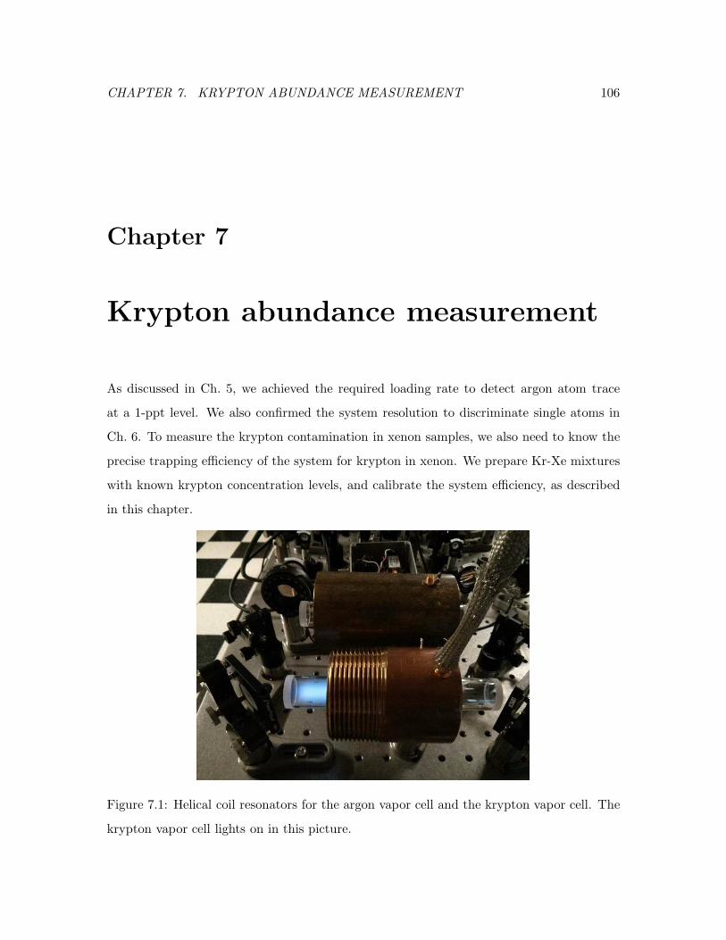
CHAPTER 7. KRYPTON ABUNDANCE MEASUREMENT 106
Chapter 7
Krypton abundance measurement
As discussed in Ch. 5, we achieved the required loading rate to detect argon atom trace
at a 1-ppt level. We also confirmed the system resolution to discriminate single atoms in
Ch. 6. To measure the krypton contamination in xenon samples, we also need to know the
precise trapping efficiency of the system for krypton in xenon. We prepare Kr-Xe mixtures
with known krypton concentration levels, and calibrate the system efficiency, as described
in this chapter.
Figure 7.1: Helical coil resonators for the argon vapor cell and the krypton vapor cell. The
krypton vapor cell lights on in this picture.

CHAPTER 7. KRYPTON ABUNDANCE MEASUREMENT 107
The system can be switched from argon trapping to krypton trapping by simply changing
the trapping laser wavelength by locking to a krypton reference cell. In the laser stabilization
system, two helical coil resonators, installed in parallel, contain a krypton vapor cell and
an argon vapor cell. We can select the paths of the probe and pump beams using flipping
mirror mounts. The angle of the grating inside the external cavity diode laser (ECDL) is
carefully adjusted with three knobs on its mount to set the wavelength range of the output
laser suitable for each transition, and the input current to the diode laser is slightly adjusted
so that the laser output is mode-hop free. As the krypton vapor cell discharge is driven
at a 70 MHz frequency (60 MHz for the argon cell), the frequency of the driving signal is
adjusted before connecting to the krypton resonator. Now the laser locks to the frequency
that is 80 MHz red-detuned from the resonant frequency of the krypton transition (λ0 =
811.5132 nm).
7.1 Measurement of krypton in argon gas
As a commissioning run of the krypton trap, we first tested the argon gas that has been used
for system adjustment. The single atom detection system was aligned using argon MOT,
then the locking frequency was changed to the krypton transition as explained above. The
detection mode was used for both trapping and detection in this measurement, which means
the loading efficiency is 1/20 of the maximum. During the measurement, the pressure in
the source chamber was maintained at 0.8 mtorr, corresponding to the consumption rate of
8× 10¹⁶/s (Sec. 5.2).
We detected 13 trapped atoms in the APD signal during a 35 minute measurement,
obtaining the loading rate of 6.2× 10⁻³ atoms/s. The trapping efficiency of the system for
krypton in argon gas has not been directly investigated. If we assume that the efficiency for
krypton in argon is same as that for argon, the krypton contamination is estimated from
the previously measured loading rate of the argon MOT and the above data by
LKr = 1.79 × 10⁸/s× 2.1 × 1
20× 0.57× Kr
Ar
= 6.2× 10⁻³/s, (7.1)
where 1.79 × 10⁸/s is the loading rate of argon MOT, 2.1 is the predicted capture ratio

CHAPTER 7. KRYPTON ABUNDANCE MEASUREMENT 108
enhancement of our Zeeman slower for krypton, 1/20 is the efficiency decrease due to using
the trapping mode, and 0.57 is the isotopic abundance of 84Kr. Solving Eq. 7.1 gives the
krypton concentration in the argon gas of 5.8× 10⁻¹⁰ (580 ppt).
If the measured trapping efficiency of the system for krypton in xenon (discussed in
Sec. 7.5) is assumed in this case, the estimated krypton concentration level, Kr/Ar, is 15
ppt. In order to derive the precise value of Kr/Ar, we need to measure the trapping efficiency
of the system for krypton in argon gas using Kr-Ar mixtures with known ratios, as we do
for krypton in xenon gas. Since the purpose of this project is to determine krypton level in
xenon gas, not in argon, further investigations of the accurate Kr/Ar value have not been
carried out. This measurement does confirm that our ATTA system works properly in the
sense of its ability to trap trace atoms in a noble gas sample and count single atoms.
7.2 Consumption rate of xenon gas
Prior to trapping krypton atoms in xenon gas, we measured the consumption rate of xenon
gas at source pressures of 0.2 mtorr to 0.8 mtorr, where the xenon discharge is active, in
the same way as discussed in Sec. 5.3. The measured consumption rates are presented in
Tab. 7.1, and plotted in Fig. 7.2. The consumption rate of xenon is about 30 % lower than
that of argon gas at the same source pressure, which is explained by the larger mass of
xenon atoms. According to the Maxwell-Boltzmann distribution for a three dimensional
gas, xenon has the most probable velocity of 193 m/s at the room temperature, while argon
has 349 m/s.
Table 7.1: Consumption rates of krypton gas for different pressures in the source chamber.
Source chamber pressure [mtorr] 0.20 0.50 0.61 0.71 0.80
Consumption rate [1016 s−1] 1.8 3.6 4.1 4.7 5.5

CHAPTER 7. KRYPTON ABUNDANCE MEASUREMENT 109
Figure 7.2: Consumption rates of xenon gas for different pressures in the source chamber.
The consumption rate increases linearly with the source chamber pressure.
7.3 Source efficiency versus pressure
The fraction of atoms that are excited by the source discharge is sensitive to the source
pressure, but it is difficult to predict the behavior theoretically. Table 7.2 presents the
relative source efficiency as a function of gas pressure, inferred from the number of atoms
detected by the APD. It is also plotted in Fig. 7.3. We find no clear relation between the
efficiency and the source pressure, but the measured data are repeatable and reliable.
Table 7.2: Relative source efficiency for krypton in xenon gas as a function of the source
pressure at a -20 dBm RF power.
Source pressure [mtorr] 0.10 0.15 0.20 0.25 0.31 0.35
Relative intensity 27 61 55 73 77 100
Source pressure [mtorr] 0.41 0.45 0.51 0.56 0.62
Relative intensity 70 68 66 64 50

CHAPTER 7. KRYPTON ABUNDANCE MEASUREMENT 110
Figure 7.3: Relative source efficiency for krypton in xenon gas in the function of the source
pressure. Blue circles are data at a −20 dBm RF power, and red circles are data at a −14
dBm RF power.
7.4 Xenon gas with high krypton contamination
A bottle of xenon gas from the XENON group at Nevis Laboratory of Columbia University
was first used for the measurement of the system efficiency for krypton in xenon gas. It
turned out to be unusable for calibration due to its high krypton level. Then another
xenon bottle was tested and it also showed too high a krypton concentration. Although
the measurements with these two bottles of xenon gas do not give us an accurate system
efficiency, they are still useful in cross-checking our calibration of the krypton concentration.
This section briefly reviews the results from these measurements.
7.4.1 Xenon bottle 1
In this test, we used a bottle of xenon gas that originated from the distillation column at
Nevis Laboratory. Since the history of the bottle was not tracked carefully, there was no
information about its krypton level. Roughly, a ppm krypton contamination was expected
before the trial. The source pressure was maintained at 0.20 mtorr, leading to a gas con-

CHAPTER 7. KRYPTON ABUNDANCE MEASUREMENT 111
sumption rate of 1.8 × 10¹⁶/s (Tab. 7.1). Operation with this xenon gas produced a large
number of trapped atoms, sufficient to form a MOT visible by a CCD camera, indicating
that the xenon bottle contains much more krypton than we expected. Calibration through
single atom detection is still possible by controlling the loading rate by a known factor, but
it involves a higher uncertainty in case of such a large loading rate.
In the image of the CCD camera, the brightness of the krypton MOT is 1/10 of that of
an argon MOT produced at the same setting. This ratio can be interpreted as a ratio of
loading rates for a large number of trapped atoms according to Eq. 5.17. ∼1 % of difference
in scattering rates between krypton and argon is ignored here. Using the system efficiency
for krypton in xenon, determined in Sec. 7.5, the krypton concentration level in the xenon
gas is estimated by1
10= 2.1 × 16.2 × 0.55 × 0.57 × Kr
Xe, (7.2)
where 1/10 is the ratio of the measured krypton loading rate compared to the argon loading
rate, 2.1 is the capture ratio enhancement for the Zeeman slower for krypton compared to
argon, 16.2 is the enhancement of the source efficiency for krypton at the source pressure
of 0.35 mtorr, 0.55 is the ratio of source efficiency between 0.20 mtorr and 0.35 mtorr, and
0.57 is the isotopic abundance of 84Kr. Equation 7.2 yields
Kr
Xe= 9.3× 10⁻³. (7.3)
This krypton level greatly exceeds our expectation.
Table 7.3: Mass components in the first bottle of xenon gas analyzed by the RGA.
Mass 1 2 14 16 17 18 28 44 64-68
Portion [%] 0.72 0.48 2.76 0.48 0.96 5.40 31.89 0.12 11.15
Mass 84 128 129 130 131 132 134 136 Total
Portion [%] 0.96 0.72 11.96 1.68 9.59 12.23 4.68 4.20 100.0
A residual gas analyzer (RGA) monitored the masses of the gas components in the
MOT chamber to verify the estimate in Eq. 7.3. The mass distribution was measured
with and without the gas flow into the system, and the background was subtracted. The

CHAPTER 7. KRYPTON ABUNDANCE MEASUREMENT 112
long distances and the vacuum pumps between the reservoir and the RGA may introduce
some errors to the data. Masses between 128 to 135 are xenon isotopes, and the masses of
64-68 indicate the xenon cracks in Tab. 7.4. The RGA data show that the gas inside the
bottle consists of 56% xenon, 32% molecular nitrogen, 5% water, 1% 84Kr, and other traces,
which means much higher impurities than expected. Although the RGA did not find other
krypton isotopes due to their low abundances, the krypton level in the bottle is derived to
1.7% according to the natural abundance of 84Kr. This is close to the estimated value from
the MOT brightness, 0.93%. The difference can arise from the uncertainty of the RGA
measurement or from different source efficiencies for xenon gas containing impurities such
as nitrogen and water.
7.4.2 Xenon bottle 2
Since the xenon bottle in Sec. 7.4.1 was not suitable for single atom detection, we ob-
tained another bottle of xenon from Nevis Laboratory, used for cold trap experiment in
the XENON group. The test was done at a 0.45 mtorr source pressure, corresponding to
a gas consumption rate of 1.8 × 10¹⁶/s (Tab. 7.1). This time, a visible krypton MOT was
formed again, with a lower intensity. The loading rate of the krypton MOT is estimated
to be 0.006 times that of argon MOT from our argon gas. The krypton level in the xenon
bottle is calculated in the same way as in Sec. 7.4.1,
0.006 = 2.1× 16.2 × 0.68× 0.57 × Kr
Xe, (7.4)
where 0.006 is the ratio of the measured krypton loading rate to the argon loading rate,
2.1 is the capture ratio enhancement for the Zeeman slower for krypton compared to argon,
16.2 is the enhancement of the source efficiency for krypton at the source pressure of 0.35
mtorr, 0.68 is the ratio of source efficiency between 0.45 mtorr and 0.35 mtorr, and 0.57 is
the isotopic abundance of 84Kr. From Eq. 7.4, Kr/Xe is calculated to be
Kr
Xe= 4.6× 10⁻⁴, (7.5)
i.e., 460 ppm.
The RGA was again used to analyze the masses of the gas components in the gas bottle
(Tab. 7.4). Xenon makes up 46%, and water 30% of the gas. The RGA data do not show

CHAPTER 7. KRYPTON ABUNDANCE MEASUREMENT 113
Table 7.4: Mass components in the second bottle of xenon gas analyzed by the RGA.
Mass 2 17 18 28 32
Portion [%] 5.52 8.29 29.83 4.42 2.21
Mass 44 64-68 129 131 132 Sum
Portion [%] 3.87 14.37 12.71 7.73 11.05 100.0
any components at the mass of krypton, which makes sense since the estimated krypton
level, 4.6 × 10⁻⁴, is too small for RGA scanning. For system calibration via single atom
detection, xenon gas less contaminated by krypton is required.
7.5 Calibration for krypton in xenon studies
After trials in Sec. 7.4, we purchased a bottle of commercial xenon gas (PraxAir) for calibra-
tion of the system efficiency for krypton in xenon. The company guarantees the minimum
purity of xenon above 99.999 % and the krypton concentration at ∼10 ppb. Table 7.5 shows
impurity levels specified in the certificate of analysis. Pure krypton gas used to make Kr-Xe
mixtures is from Spectra Gases Inc.
Table 7.5: Specified impurity levels of the xenon bottle from PraxAir.
Components Oxygen Nitrogen THC Water CO2 Krypton Ar, H2
Concentration [ppb] 100 440 100 100 100 10 400
The gas mixing system consists of a 201 cm3 chamber where krypton gas is filled and
a 221 cm3 reservoir where krypton and xenon gases are mixed (Figure. 7.4). Including the
volume of connections to each of them, the confinement volumes of the krypton chamber
and the mixing region are 260 cm3 and 766 cm3, respectively. To prepare Kr-Xe mixtures
at arbitrary concentrations, all connections to the krypton chamber, except for one to the
krypton gas bottle, are closed, and krypton gas is introduced at a low pressure. The pressure
of the krypton gas is monitored by a capacitive manometer (Pfeiffer Vacuum CMR 365)
connected to the krypton chamber. Then the connection to the krypton bottle is closed and

CHAPTER 7. KRYPTON ABUNDANCE MEASUREMENT 114
the remaining krypton gas outside the krypton chamber is pumped out through a bypassing
pipe. Once the pressure is close to the asymptotic limit, the xenon gas bottle and the valve
between the reservoir and the krypton chamber are opened, and the krypton and xenon
gases are mixed by dispersion. A pressure transducer is used to read the pressure in the
gas mixing region.
Figure 7.4: Schematic of the gas inlet system and image of the krypton chamber and its
connections. Krypton gas in the small krypton chamber is mixed with xenon gas in the
reservoir. A pressure transducer (D) and a capacitive manometer (C) monitor the pressure
in the reservoir and in the mixing volume, respectively (left). A fine leak valve controls the
amount of krypton gas in the krypton chamber (right).
In this section, we determine the trapping efficiency of our system for krypton in xenon
gas, based on single atom measurement with two different Kr-Xe mixtures. This is the last
test required prior to measuring krypton contamination in xenon samples. Additionally,
the krypton level in the xenon gas from PraxAir is estimated from these measurements.

CHAPTER 7. KRYPTON ABUNDANCE MEASUREMENT 115
7.5.1 Pure xenon gas from PraxAir
Before measurements with Kr-Xe mixtures, the pure xenon gas from PraxAir was tested.
At the time of this measurement, the loading rate measured with argon MOT was half of
the maximum. Additionally, all transverse cooling stages were switched off to reduce the
loading rate, since a ppb level of krypton is expected to generate too many trapped atoms.
The source was maintained at a 0.20 mtorr pressure, corresponding to the consumption rate
of 1.8× 10¹⁶/s.
The APD detected 52 trapped atoms in 20 minutes, leading to the loading rate of
4.3× 10⁻²/s. By adjusting this number to the optimized setting of our system, we have the
loading rate
LPraxAir = 4.3× 10⁻²/s× 2× 12× 1
0.55= 1.88/s (+25%
−22%), (7.6)
where 4.3 × 10⁻²/s is the measured loading rate, 2 is from the non-optimized loading rate
at the time of the measurement with an uncertainty of ±3%, 12 is the transverse cooling
enhancement factor with an uncertainty of ±5%, and 1/0.55 is the ratio of source efficiency
between 0.20 mtorr and 0.35 mtorr with an uncertainty of ±10%.
7.5.2 12 ppm krypton mixture
The krypton chamber was filled with krypton gas at 2.2 mtorr, then mixed with xenon gas
at 15.4 torr in the mixing region, leading to a 12 ppm (±5%) Kr/Xe level estimated from
the specified volumes of each region. The source was operated at the pressure of 0.2 mtorr,
i.e., the consumption rate of 1.8× 10¹⁶/s. For single atom detection, the loading rate needs
to be reduced by a known amount for the reason discussed in Sec. 7.5.1. For this purpose,
the Zeeman slower laser was partially blocked with a small aperture, and all transverse
cooling stages were blocked. Additionally, one transverse cooling laser was used in a one
way configuration to push the atomic beam.
The time taken to find 100 single atoms from the APD signal was measured to be 147
seconds, which is equivalent to 0.68 atoms/s. By compensating for the efficiency decrease
CHAPTER 7. KRYPTON ABUNDANCE MEASUREMENT 116
mentioned above, the loading rate for a 12 ppm Kr/Xe gas is estimated as
L12ppm Kr = 0.68 /s× 1
0.3× 12× 3
2× 1
0.03× 1
0.55
= 2.47 × 10³ /s (+32%−26%
), (7.7)
where 0.68/s is the measured loading rate, 1/0.3 is due to the non-optimized loading rate
at the time of the measurement with an uncertainty of ±3%, 12 is the transverse cooling
enhancement factor with an uncertainty of ±5%, 3/2 is the effect of the one way laser
pushing the atomic beam with an uncertainty of ±3%, 1/0.03 is compensation of the small
aperture on the Zeeman slower laser with an uncertainty of ±8%, and 1/0.55 is the ratio of
source efficiency between 0.20 mtorr and 0.35 mtorr with an uncertainty of ±10%.
From Eq. 7.7, the loading rate of a 1-ppt Kr/Xe gas is
L1ppt Kr = 2.06× 10⁻⁴/s (+39%−30%
). (7.8)
This loading rate implies that 81 minutes are required to detect one trapped atom from a
1-ppt Kr/Xe gas. Comparing this to the loading rate of the PraxAir xenon gas, 1.88/s, the
krypton level in the xenon gas is estimated to be 9.1 ppb.
7.5.3 0.75 ppm krypton mixture
For the next measurement, a 0.75 ppm (±5%) Kr/Xe mixture was prepared by filling the
krypton chamber with krypton gas and the reservoir with xenon gas at 57.0 torr in the
mixing region. The source pressure was 0.2 mtorr as before, and the loading rate of the
argon MOT was at the maximum value. The overall loading rate was controlled by switching
off transverse cooling stages and partially blocking the Zeeman slower laser.
We found 24 trapped atoms in 150 seconds from APD measurement, indicating the
loading rate of 0.16 atoms/s. Adjustment for the optimal setting predicts the best loading
rate of the 0.75 ppm Kr/Xe mixture as
L0.75ppm Kr = 0.16/s × 12× 1
0.03× 1
0.55
= 1.16 × 10²/s (+25%−21%
), (7.9)
where 0.16/s is the measured loading rate, 12 is the enhancement by transverse cooling with
an uncertainty of ±5%, 1/0.03 is compensation of the small aperture on the Zeeman slower

CHAPTER 7. KRYPTON ABUNDANCE MEASUREMENT 117
laser with an uncertainty of ±8%, and 1/0.55 is the ratio of source efficiency between 0.20
mtorr and 0.35 mtorr with an uncertainty of ±10%.
Equation 7.9 implies that the loading rate for a 1 ppt Kr/Xe gas is
L1ppt Kr = 1.55 × 10⁻⁴ /s (+30%−25%
), (7.10)
corresponding to a measurement time of 108 minutes to detect one trapped atom. This
measurement indicates in a 12.1-ppb krypton level of the PraxAir xenon gas.
7.5.4 System efficiency for krypton in xenon
By averaging results from the 12 ppm and 0.75 ppm Kr/Xe mixtures, we have a loading
rate for 1 ppt krypton contamination in xenon gas,
L1ppt Kr = 1.80 × 10⁻⁴ /s (+35%−28%
). (7.11)
With this loading rate, the average time required to find one trapped atom from a 1 ppt
Kr/Xe sample is estimated to be 92 minutes, which is a reasonable amount of time since
we can expect ∼6 atoms for a one-day measurement.
The krypton level in the PraxAir xenon gas is also calculated from the derived loading
rate byKr
Xe= 10−12 × LPraxAir
L1ppt Kr= 1.04 × 10⁻⁸ (+21%
−17%), (7.12)
i.e., 10.4 ppb. This number is very close to the impurity level specified by the company, 10
ppb.
7.6 Xenon extraction from the XENON detector
As the trapping efficiency of our ATTA system for krypton in xenon is determined (Sec. 7.5),
we are ready to measure the krypton level in a xenon sample from the XENON100 detector,
which is the goal of this project. A gas container, called ‘gas pipette’, was built to extract
and carry the xenon sample from the INFN Laboratori Nazionali del Gran Sasso (LNGS)
to the laboratory at Columbia University.
The gas pipette consists of a one liter stainless steal vessel (MDC 43000-2000), an all-
metal ultra-fine leak valve (Lesker VZLVM940R), and a shutoff valve as shown in Fig. 7.5.

CHAPTER 7. KRYPTON ABUNDANCE MEASUREMENT 118
Figure 7.5: A pipette to extract and carry xenon gas from the XENON100 detector.
Two valves are employed to make sure that the piece is leak-tight. After the pipette was
assembled, it was baked at 300 C for several days to remove water and other impurities,
and shipped to the LNGS.

CHAPTER 8. CONCLUSION 119
Chapter 8
Conclusion
As described in this thesis, we have built an atom trap trace analysis (ATTA) system to
measure krypton contamination levels in the XENON dark matter detectors. The ATTA
system traps and counts the contaminant atoms within the target, using standard cooling
and trapping techniques, including transverse cooling, Zeeman slowing, and a magneto-
optical trap (MOT).
By carefully optimizing the system, we achieved the loading efficiency required to detect
krypton contamination in xenon samples within a reasonable amount of measurement time.
Fluorescence photons emitted from trapped atoms are detected by an avalanche photodiode
(APD). With a specially designed optical system, we obtained a signal-to-noise ratio (SNR)
sufficient to discriminate single atoms signals from background noise.
The precise system efficiency for krypton in xenon gas was determined by testing the
system with Kr-Xe mixtures at 0.75 ppm and 12 ppm. With the measured system effi-
ciency, we expect to find one trapped 84Kr atom at a 1-ppt Kr/Xe level in a ∼90 minute
measurement. A test with commercial xenon gas, whose krypton level is specified as ∼10
ppb, estimates a 10.6-ppb krypton concentration, validating that our ATTA apparatus.
The system is ready for measurements when a xenon sample is available upon termina-
tion of the current dark matter detection run. The achieved loading efficiency is acceptable
for a measurement of a 1-ppt krypton contamination, but the higher efficiency will allow us
more precise result from a short-time measurement. Additionally, as XENON1T aims for
a sub-ppt krypton level in its xenon target, increase of the system efficiency is desired for

CHAPTER 8. CONCLUSION 120
future. There are several approaches for the efficiency improvement.
As discussed in Sec. 6.3.2, using the detection mode laser beam decreases the loading
efficiency by 1/20 compared to the trapping mode beam. By switching two modes quickly,
we can compensate for the decrease while maintaining the low background for the APD
detection. Due to the loss of the detection period from mode switching, the actual en-
hancement will be less than by a factor of 20, but we still expect ∼10. The two modes
can be switched by splitting one MOT laser beam into the trapping and detection beams,
and blocking/unblocking each beam using mechanical shutters. It can also be done by a
commercial laser power controller.
Increasing the gas cooling power will lead to more atoms below the capture velocity of
the Zeeman slower, improving the Zeeman slower efficiency. Building a new Zeeman slower
with a longer length can increase the capture fraction. However, these methods are not
able to increase the system efficiency significantly since the capture fraction of the Zeeman
slower already reached 66%.
For a long-term plan, an optical excitation methods discussed in Sec. 4.3.1 will allow
us to reach a higher excitation efficiency as well as stabilize the source behavior. The
non-resonant UV+UV excitation method (Fig. 4.6 (middle)) is under discussion, where the
215 nm wavelength is obtained from a diode or Ti:Sapphire laser by nonlinear frequency
conversion. We expect the enhancement by a factor of up to 100 from the modification.

BIBLIOGRAPHY 121
Bibliography
[Abbasi et al., 2011] R. Abbasi, Y. Abdou, T. Abu-Zayyad, J. Adams, et al. Measurement
of the atmospheric neutrino energy spectrum from 100 gev to 400 tev with icecube. Phys.
Rev. D, 83:012001, 2011.
[Ade et al., 2013] P. A. R. Ade, N. Aghanim, C. Armitage-Caplan, M. Arnaud, et al. Planck
2013 results. XVI. Cosmological parameters. ArXiv, 1303.5076, 2013.
[Ageron et al., 2011] M. Ageron, J.A. Aguilar, I. Al Samarai, A. Albert, et al. ANTARES:
The first undersea neutrino telescope. Nuclear Instruments and Methods in Physics Re-
search Section A, 656(1):11 – 38, 2011.
[Ahlswede et al., 2013] Jochen Ahlswede, Simon Hebel, J. Ole Ross, Robert Schoetter, et al.
Update and improvement of the global krypton-85 emission inventory. Journal of Envi-
ronmental Radioactivity, 115:34–42, 2013.
[Ahmed et al., 2010] Z. Ahmed, D. S. Akerib, S. Arrenberg, C. N. Bailey, et al. Dark Matter
Search Results from the CDMS II Experiment. Science, 327(5973):1619–1621, 2010.
[Alt, 2002] Wolfgang Alt. An objective lens for efficient fluorescence detection of single
atoms. Optik - International Journal for Light and Electron Optics, 113(3):142 – 144,
2002.
[Alton et al., 2009] D. Alton, D. Durben, M. Keeter, K. Zehfus, et al. DarkSide-50: A
direct search for dark matter with new techniques for reducing background. Technical
report, 2009.
BIBLIOGRAPHY 122
[Angloher et al., 2012] G. Angloher, M. Bauer, I. Bavykina, A. Bento, et al. Results from
730 kgdays of the CRESST-II Dark Matter search. The European Physical Journal C,
72(4):1–22, 2012.
[Aprile and Doke, 2010] E. Aprile and T. Doke. Liquid xenon detectors for particle physics
and astrophysics. Reviews of Modern Physics, 82(3):2053–2097, 2010.
[Aprile and Zelevinsky, 2009] E. Aprile and T. Zelevinsky. Instrument development for
liquid xenon dark matter searches: an atom trap trace analysis system to measure ultra-
low krypton contamination in xenon. NSF award, #0923274, 2009.
[Aprile et al., 2006] E. Aprile, C. E. Dahl, L. de Viveiros, R. J. Gaitskell, et al. Simultaneous
measurement of ionization and scintillation from nuclear recoils in liquid xenon for a dark
matter experiment. Phys. Rev. Lett., 97:081302, 2006.
[Aprile et al., 2010] E. Aprile, K. Arisaka, F. Arneodo, A. Askin, et al. First dark matter
results from the XENON100 experiment. Phys. Rev. Lett., 105:131302, 2010.
[Aprile et al., 2011] E. Aprile, K. Arisaka, F. Arneodo, A. Askin, et al. Study of the electro-
magnetic background in the XENON100 experiment. Physical Review D, 83(8):082001,
2011.
[Aprile et al., 2012a] E. Aprile, M. Alfonsi, K. Arisaka, Arneodo, et al. Dark matter results
from 225 live days of XENON100 data. Phys. Rev. Lett., 109:181301, 2012.
[Aprile et al., 2012b] E. Aprile, K. Arisaka, F. Arneodo, A. Askin, et al. The XENON100
dark matter experiment. Astroparticle Physics, 35(9):573 – 590, 2012.
[Armengaud et al., 2012] E. Armengaud, C. Augier, A. Benoˆ, L. Berge, et al. Search
for low-mass WIMPs with EDELWEISS-II heat-and-ionization detectors. Phys. Rev. D,
86:051701, 2012.
[Bartlett, 1962] N Bartlett. Xenon hexafluoroplatinate(V) Xe+[PtF6]−. Proc. Chem. Soc.,
page 218, 1962.

BIBLIOGRAPHY 123
[Begeman et al., 1991] K. G. Begeman, A. H. Broeils, and R. H. Sanders. Extended rotation
curves of spiral galaxies: dark haloes and modified dynamics. Mon. Not. R. Astr. Soc.,
249:523–537, 1991.
[Bertone et al., 2005] Gianfranco Bertone, Dan Hooper, and Joseph Silk. Particle dark
matter: evidence, candidates and constraints. Physics Reports, 405(5-6):279–390, 2005.
[Bertone, 2010] Gianfranco Bertone. The moment of truth for WIMP dark matter. Nature,
468(7322):389–93, 2010.
[Bjorklund and Levenson, 1981] G. C. Bjorklund and M. D. Levenson. Sub-Doppler
frequency-modulation spectroscopy of I2. Phys. Rev. A, 24:166–169, 1981.
[Bradac et al., 2008] Marusa Bradac, Steven W. Allen, Tommaso Treu, Harald Ebeling,
et al. Revealing the properties of dark matter in the merging cluster macs j0025.41222.
The Astrophysical Journal, 687(2):959, 2008.
[Carr et al., 2006] J. Carr, G. Lamanna, and J. Lavalle. Indirect detection of dark matter.
Reports on Progress in Physics, 69(8):2475, 2006.
[Cartledge et al., 2008] Stefan I. B. Cartledge, J. T. Lauroesch, David M. Meyer, Ulysses J.
Sofia, et al. Interstellar krypton abundances: The detection of kiloparsec-scale differences
in galactic nucleosynthetic history. The Astrophysical Journal, 687(2):1043, 2008.
[Chen et al., 1999] C. Y. Chen, Y. M. Li, K. Bailey, T. P. O’Connor, et al. Ultrasensitive
isotope trace analyses with a magneto-optical trap. Science, 286(5442):1139–41, 1999.
[Chen et al., 2001] C. Y. Chen, K. Bailey, Y. M. Li, T. P. O’Connor, et al. Beam of
metastable krypton atoms extracted from a rf-driven discharge. Rev. Sci. Inst., 72(1):271–
272, 2001.
[Clowe et al., 2004] Douglas Clowe, Anthony Gonzalez, and Maxim Markevitch. Weak-
lensing mass reconstruction of the interacting cluster 1e 0657558: Direct evidence for the
existence of dark matter. The Astrophysical Journal, 604(2):596, 2004.

BIBLIOGRAPHY 124
[Clowe et al., 2006] Douglas Clowe, Marusa Bradac, Anthony H. Gonzalez, Maxim Marke-
vitch, et al. A direct empirical proof of the existence of dark matter. The Astrophysical
Journal Letters, 648(2):L109, 2006.
[Du, 2003] Xu Du. Realization of radio-krypton dating with an atom trap. PhD thesis,
Northwestern University, 2003.
[Ekwurzel et al., 1994] Brenda Ekwurzel, Peter Schlosser, William M. Smethie, L. Niel
Plummer, et al. Dating of shallow groundwater: Comparison of the transient tracers
3H/3He, chlorofluorocarbons, and 85Kr. Water Resources Research, 30(6):1693–1708,
1994.
[Elmer, 2007] Perkin Elmer. Single Photon Counting Module SPCM-AQRH series data
sheet. Fremont, CA, 2007.
[Feng, 2010] Jonathan L. Feng. Dark matter candidates from particle physics and methods
of detection. Annual Review of Astronomy and Astrophysics, 48(1):495–545, 2010.
[Fixsen, 2009] D. J. Fixsen. The temperature of the cosmic microwave background. The
Astrophysical Journal, 707(2):916, 2009.
[Foot, 2005] C.J. Foot. Atomic physics. Oxford master series in physics. Oxford University
Press, 2005.
[Friedman et al., 1967] H. Friedman, E. T. Byram, and T. A. Chubb. Distribution and
variability of cosmic X-ray. Science, 156:374–378, 1967.
[Gaitskell, 2004] Richard J. Gaitskell. Direct detection of dark matter. Annual Review of
Nuclear and Particle Science, 54(1):315–359, 2004.
[Glatz, 1996] Joseph Glatz. Krypton gas penetrant imaging – a valuable tool for ensuring
structural integrity in aircraft engine components. Materials Evaluation, 54:1352–1362,
1996.
[Gordon and Selvin, 2003] Matthew P. Gordon and Paul R. Selvin. A microcontroller-based
failsafe for single photon counting modules. Review of Scientific Instruments, 74(2):1150,
2003.

BIBLIOGRAPHY 125
[Hall, 1981] J. L. Hall. Optical heterodyne saturation spectroscopy. Applied Physics Letters,
39(9):680, 1981.
[Haynes, 2013] William M. Haynes, editor. CRC handbook of chemistry & physics. CRC
Press, 94th edition, 2013.
[Hippel et al., 1985] Frank Von Hippel, David H Albright, and Barbara G Levi. Stopping
the production of fissile materials for weapons. Scientific American, 253:40–47, 1985.
[Hitachi, 2005] Akira Hitachi. Properties of liquid xenon scintillation for dark matter
searches. Astroparticle Physics, 24(3):247–256, 2005.
[Jortner et al., 1965] Joshua Jortner, Lothar Meyer, Stuart A. Rice, and E. G. Wilson.
Localized excitations in condensed Ne, Ar, Kr, and Xe. The Journal of Chemical Physics,
42(12):4250, 1965.
[Jungman et al., 1996] Gerard Jungman, Marc Kamionkowski, and Kim Griest. Supersym-
metric dark matter. Physics Reports, 267(56):195–373, 1996.
[Kane and Watson, 2008] Gordon Kane and Scott Watson. Dark matter and LHC: What
is the connection? Modern Physics Letters A, 23(26):2103–2123, 2008.
[Levin and Hesshaimer, 1996] Ingeborg Levin and Vago Hesshaimer. Refining of atmo-
spheric transport model entries by the globally observed passive tracer distributions of 85
krypton and sulfur hexafluoride (SF6). Journal of Geophysical Research, 101(16):745–755,
1996.
[Lewis et al., 2003] Aaron D. Lewis, David A. Buote, and John T. Stocke. Chandra obser-
vations of a2029: The dark matter profile down to below 0.01rvir in an unusually relaxed
cluster. The Astrophysical Journal, 586(1):135, 2003.
[Lim, 2013] Kyungen Lim. XENON100 Dark Matter Search : Scintillation Response of
Liquid Xenon to Electronic Recoils. PhD thesis, Columbia University, 2013.
[Linde Electronics and Specialty Gases, 2010] Linde Electronics and Specialty Gases. Mul-
tipurpose analog PID controller. Technical report, The Linde Group, 2010.

BIBLIOGRAPHY 126
[Lindemann and Simgen, 2013] S. Lindemann and H. Simgen. Krypton assay in xenon at
the ppq level using a gas chromatographic system combined with a mass spectrometer.
ArXiv, 1308.4806, 2013.
[Liu and Littman, 1981] Karen Liu and Michael G. Littman. Novel geometry for single-
mode scanning of tunable lasers. Opt. Lett., 6(3):117–118, 1981.
[Macalpine and Schildknecht, 1959] W. W. Macalpine and R. O. Schildknecht. Coaxial
resonators with helical inner conductor. Proc. IRE, 47:2099, 1959.
[Marcassa et al., 1993] L. Marcassa, V. Bagnato, Y. Wang, C. Tsao, et al. Collisional loss
rate in a magneto-optical trap for sodium atoms: Light-intensity dependence. Phys. Rev.
A, 47:R4563–R4566, 1993.
[Marchionni et al., 2011] A Marchionni, C Amsler, A Badertscher, V Boccone, et al. ArDM:
a ton-scale LAr detector for direct Dark Matter searches. Journal of Physics: Conference
Series, 308(1):012006, 2011.
[McDougall, 1999] Ian McDougall, editor. Geochronology and thermochronology by the
40Ar/39Ar method. New York : Oxford University Press, 2nd edition, 1999.
[McKinsey and Orzel, 2005] D.N. McKinsey and C. Orzel. Radioactive krypton background
evaluation using atom counting. Nuclear Instruments and Methods in Physics Research
Section A: Accelerators, Spectrometers, Detectors and Associated Equipment, 545(12):524
– 531, 2005.
[McKinsey et al., 2010] D N McKinsey, D Akerib, S Bedikian, A Bernstein, et al. The LUX
dark matter search. Journal of Physics: Conference Series, 203(1):012026, 2010.
[Metcalf and van der Straten, 1999] H.J. Metcalf and P. van der Straten. Laser cooling and
trapping. Graduate Texts in Contemporary Physics. Springer-Verlag GmbH, 1999.
[Meyrath, 2005] Todd P. Meyrath. Multipurpose analog PID controller. Technical report,
University of Texas at Austin, 2005.
[Ovchinnikov, 2008] Y. B. Ovchinnikov. A permanent Zeeman slower for Sr atomic clock.
The European Physical Journal Special Topics, 163(1):95–100, 2008.

BIBLIOGRAPHY 127
[Penzias and Wilson, 1965] A. A. Penzias and R. W. Wilson. A measurement of excess
antenna temperature at 4080 Mc/s. The Astrophysical Journal, 142:419–421, 1965.
[Phillips and Metcalf, 1982] William D. Phillips and Harold Metcalf. Laser deceleration of
an atomic beam. Phys. Rev. Lett., 48:596–599, 1982.
[Plante, 2012] Guillaume Plante. The XENON100 dark matter experiment: design, con-
struction, calibration and 2010 search results with improved measurement of the scin-
tillation response of liquid xenon to low-energy nuclear recoils. PhD thesis, Columbia
University, 2012.
[Prodan and Phillips, 1984] John V. Prodan and William D. Phillips. Chirping the light-
fantastic? Recent NBS atom cooling experiments. Progress in Quantum Electronics,
8(34):231 – 235, 1984.
[Reinaudi et al., 2012] G. Reinaudi, C. B. Osborn, K. Bega, and T. Zelevinsky. Dynamically
configurable and optimizable Zeeman slower using permanent magnets and servomotors.
J. Opt. Soc. Am. B, 29(4):729–733, 2012.
[Rentzepis and Douglass, 1981] P. M. Rentzepis and D. C. Douglass. Xenon as a solvent.
Nature, 293:165, 1981.
[Schroder et al., 1971] J. Schroder, K. O. Munnich, and D. H. Ehhalt. Krypton-85 in the
troposphere. Nature, 233(29):614, 1971.
[Steane et al., 1992] A. M. Steane, M. Chowdhury, and C. J. Foot. Radiation force in the
magneto-optical trap. J. Opt. Soc. Am. B, 9(12):2142–2158, 1992.
[Sukenik and Busch, 2002] C. I. Sukenik and H. C. Busch. A rf discharge cell for saturated
absorption spectroscopy of metastable argon. Rev. Sci. Inst., 73(2):493–494, 2002.
[Taylor and Thompson, 2008] Barry Taylor and Ambler Thompson. The international sys-
tem of units (si). Technical report, NIST, 2008.
[Yamashita et al., 2004] M. Yamashita, T. Doke, K. Kawasaki, J. Kikuchi, and S. Suzuki.
Scintillation response of liquid Xe surrounded by PTFE reflector for gamma rays. Nuclear

BIBLIOGRAPHY 128
Instruments and Methods in Physics Research Section A: Accelerators, Spectrometers,
Detectors and Associated Equipment, 535(3):692 – 698, 2004.
[YanQiang et al., 2012] Guo YanQiang, Li Gang, Zhang YanFeng, Zhang PengFei, et al.
Efficient fluorescence detection of a single neutral atom with low background in a micro-
scopic optical dipole trap. Science China Physics, Mechanics & Astronomy, 55(9):1523,
2012.
[Young et al., 2002] L. Young, D. Yang, and R. W. Dunford. Optical production of
metastable krypton. Journal of Physics B: Atomic, Molecular and Optical Physics,
35(13):2985, 2002.
[Ziegler and Nichols, 1942] J. G. Ziegler and N. B. Nichols. Optimum settings for automatic
controllers. Trans. ASME, 64:759–768, 1942.
[Zwicky, 1933] F. Zwicky. Spectral displacement of extra galactic nebulae. Helv. Phys.
Acta, 6:110–127, 1933.