Alkaline Surfactant Polymer Enhanced Oil Recovery Process · Alkaline Surfactant Polymer Enhanced...

RICE UNIVERSITY

Alkaline Surfactant Polymer Enhanced Oil Recovery Process

by

Shunhua Liu

DOCTOR OF PHILOSOPHY

DECEMBER, 2007

RICE UNIVERSITY


by Shunhua Liu

A THESIS SUBMITTED

IN PARTIAL FULFILLMENT OF THE REQUIREMENTS FOR THE DEGREE

DOCTOR OF PHILOSOPHY

APPROVED, THESIS COMMITTEE:

Dr. Clarence A. Miller, Louis Calder Professor of Chemical Engineering, Co-chair

Dr. George J. Hirasaki, A. J. Hartsook Professor of Chemical Engineering, Co-chair

Dr. Walter G. Chapman, William W. Akers Professor of Chemical Engineering

Dr. Mason B. Tomson, Professor of Civil and Environmental Engineering

Maura C. Puerto, Complimentary Visiting Scholar in Chemical Engineering

HOUSTON, TEXAS

January, 2008

i

ABSTRACT


by

Shunhua Liu

This thesis improves the understanding of the Alkaline Surfactant Polymer (ASP)

enhanced oil recovery process in order to optimize the ASP operational strategy. The

conventional oil recovery methods leave large amounts of oil in the reservoir. ASP

process is considered as a promising method for enhanced oil recovery. This dissertation

reveals the ASP characteristics by using phase behavior, interfacial tension, surfactant

consumption and numerical simulation techniques. The flooding experiments that I

performed show that my ASP strategies successfully recover the oil trapped after

waterflooding.

The optimal salinity varies when either synthetic surfactant concentration or

Water Oil Ratio (WOR) changes in ASP system. In this thesis, these results could be

collapsed to a single curve for each synthetic surfactant/crude oil combination in which

the optimal salinity depends only on the molar ratio of natural soap to synthetic surfactant,

or soap fraction of total soap plus surfactant.

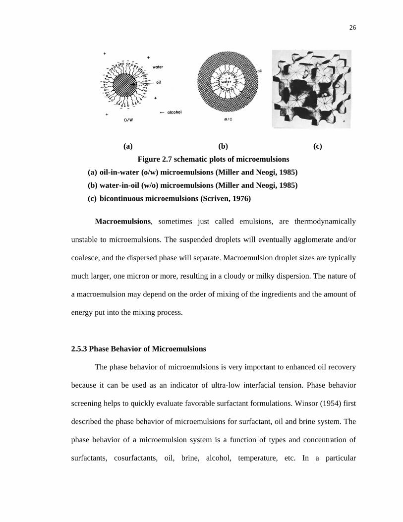
The ASP system studied here has a much wider low IFT region (< 0.01 mN/m)

than the system without alkali. In much of the Winsor I region where an oil-in-water

microemulsion coexists with excess oil, a second surfactant-containing phase was seen to

exist in colloidal form. This colloidal dispersion plays an important role in reaching the

ultra-low tension. A new protocol, which significantly reduces the time that is required to

ii

reach equilibrium, is developed to assure that enough of the dispersed material is initially

present to achieve low tensions but not so much as to obscure the oil drop during IFT

measurements.

Surfactant retention is one of the most significant barriers to the commercial

application of ASP. It was found that Na2CO3 but not NaOH or Na2SO4, can substantially

reduce adsorption of anionic surfactants on carbonate formations, especially at low

salinities.

A one-dimensional numerical simulator was developed to model the ASP process.

By calculating transport of water, oil, surfactant, soap, salt, alkali and polymer, the

simulations show that a gradient in soap-to-surfactant ratio develops with conditions

shifting from over-optimum ahead of the displacement front to under-optimum behind

the displacement front. This gradient makes the process robust and permits injection at

conditions well below optimal salinity of the synthetic surfactant, thereby reducing

adsorption and improving compatibility with polymer.

More than 95% of waterflood residual oil was recovered in ASP sand pack

experiments at ambient temperature with a slug containing a partially hydrolyzed

polyacrylamide polymer and only 0.2 wt% of a particular anionic surfactant blend. The

simulator predicts recovery curves in agreement with those found in the flooding

experiments.

iii

ACKNOWLEGEMENTS

I am very grateful as a graduate student at Rice University. I would like to express

my sincere appreciation to my two advisors, Professor Clarence A. Miller and Professor

George J. Hirasaki for their guidance, inspiration, and assistance. Their wisdom and

authoritative knowledge have helped me a lot throughout these years.

I want to give special thanks to Maura C. Puerto for her valuable recommendation,

suggestion and help.

I appreciate Professor Mason Tomson and Professor Walter Chapman for serving

on my thesis committee.

Many research staffs, graduates and undergraduates have contributed with their

experimental work and/or valuable ideas to this thesis. I want to especially thank Leslie

Zhang for teaching me phase behavior and IFT experimental skills, Brent Biseda for

making a lot of adsorption and IFT measurements, Dick Chronister for repairing old

spinning drop machine and other experimental apparatus, Will Knowles for helping me

with the BET analysis. I also want to thank to Arjun Kurup, Wei Yan, Busheng Li,

Tianmin Jiang, Robert Li, Jie Yu, Nick Parra-Vasque for all their help with the laboratory

experiments. Many other students and research staff in Dr. Miller’s and Dr. Hirasaki’s

laboratories have offered me help and their friendships too. I am grateful to this group of

people.

I would give many thanks to Dr. Gary Pope and Dr. Mojdeh Delshad, as well as

their students at University of Texas at Austin, for those valuable suggestions on DOE

iv

projects. I also thank Dr. Varadarajan Dwarakanath from Chevron, Professor Kishore

Mohanty and his student at University of Houston for the discussions.

I acknowledge U.S. DOE and Consortium on Processes in Porous Media at Rice

University for the financial support. Thanks to Stepan, Kirk Raney from Shell Chemical

for providing surfactant chemicals and SNF Company for polymer.

At the end, I would like to thank my family for their support and encouragement.

v

TABLE OF CONTENTS

List of Figures ......................................................................................................................x

List of Tables .................................................................................................................. xvii

Chapter1: Introduction .........................................................................................................1

1.1: General background and motivation.......................................................................1

2.2: Summary of chapters ..............................................................................................3

Chapter 2: Concepts and Techniques on Alkaline Surfactant Polymer Process..................5

2.1: Enhanced Oil Recovery ..........................................................................................5

2.2: Concepts on Alkaline surfactant polymer Process .................................................7

2.2.1 Darcy’s Law....................................................................................................7

2.2.2 Interfacial Tension ..........................................................................................9

2.2.3 Wettability.......................................................................................................9

2.2.4 Capillary Pressure .........................................................................................11

2.2.5 Flooding and Imbibition ...............................................................................12

2.3: Enhanced Oil Recovery Mechanisms ...................................................................12

2.4: Alkali Enhanced Oil Recovery .............................................................................16

2.5: Surfactant Enhanced Oil Recovery.......................................................................20

2.5.1 Surfactants.....................................................................................................21

2.5.2 Surfactant Micelle and Microemulsion.........................................................23

2.5.3 Phase Behavior of Microemulsions ..............................................................26

2.5.4 Phase Behavior and Interfacial Tension .......................................................30

2.5.5 Surfactant Retention......................................................................................32

2.5.5.1 Surfactant Adsorption on Mineral Surface ..........................................32

2.5.5.2 Surfactant Precipitation........................................................................33

2.5.5.3 Phase Trapping.....................................................................................34

2.5.6 Co-solvents in Surfactant Process.................................................................36

2.5.7 Cationic Surfactant Flooding ........................................................................37

2.6: Mobility Control in Enhanced Oil Recovery........................................................38

vi

2.6.1 Polymer Process............................................................................................38

2.6.2 Foam Process ................................................................................................40

2.7: Alkaline Surfactant Polymer Enhanced Oil Recovery .........................................40

2.8: Numerical Simulation ...........................................................................................43

Chapter 3: Phase Behaviors of Alkaline Surfactant System..............................................45

3.1: Materials ...............................................................................................................45

3.1.1 Surfactant Selection ......................................................................................45

3.1.2 Crude Oils .....................................................................................................48

3.1.3 Other Chemicals............................................................................................48

3.2: Soap Extraction for crude oils ..............................................................................49

3.3: Phase behavior Experimental Procedure ..............................................................51

3.4: Phase behavior Results .........................................................................................52

3.4.1 Phase Behavior of PBB and NI Blend ..........................................................52

3.4.2 Phase Behavior of Yates and NI Blend.........................................................58

3.4.3 Phase Behavior of SWCQ and NI Blend ......................................................62

3.4.4 Phase Behavior of Pure Hydrocarbons and NI Blend...................................63

3.4.5 Birefringence of MY4-NI Blend system.......................................................67

Chapter 4: Interfacial Tension (IFT) Properties of Alkaline Surfactant System ...............69

4.1: IFT Measurement Methods...................................................................................69

4.1.1 Pendant Drop Method...................................................................................69

4.1.2 Spinning Drop Method .................................................................................72

4.2: Interfacial Tension of Crude Oil and Brine ..........................................................74

4.3: Interfacial Tension of Alkaline Surfactant Systems .............................................75

4.3.1 Interfacial Tension and Colloidal Dispersion of Alkaline Surfactant System..

................................................................................................................................75

4.3.2 Spinning Drop IFT Experimental Protocol for Alkaline Surfactant Crude

System ...................................................................................................................80

4.3.3 Width of Low IFT Region of Alkaline Surfactant System ..........................83

4.3.4 Correlation between Phase Behavior and IFT .............................................84

vii

4.3.5 Dynamic IFT and equilibrium IFT ..............................................................89

Chapter 5: Chemical Consumptions of Alkaline Surfactant Process.................................92

5.1: Static Adsorption of Surfactant.............................................................................92

5.1.1 Static Adsorption Experimental Procedure...................................................92

5.1.2 Static Adsorption Results for Anionic surfactant .........................................93

5.1.2.1 TC Blend..............................................................................................93

5.1.2.2 Test of Other Potential Determining Ions............................................95

5.1.2.3 Surfactant Adsorption on Different Surface Area ...............................96

5.1.2.4 NI Blend...............................................................................................98

5.1.2.5 Adsorption of Nonionic Surfactant and Anionic Surfactant..............103

5.2: Dynamic Adsorption of Surfactant .....................................................................105

5.2.1 Dynamic Adsorption Experimental Procedure ...........................................106

5.2.2 Dynamic Adsorption Model .......................................................................107

5.2.3 Dynamic Adsorption of Anionic Surfactant ...............................................111

5.3: Sodium Carbonate Consumption by Gypsum ....................................................116

Chapter 6: Simulation and Optimization of Alkaline Surfactant Polymer Process .........119

6.1: One-dimensional Simulator ................................................................................119

6.1.1 Assumptions and Models............................................................................120

6.1.1.1 Surfactant and Soap Partitioning .......................................................121

6.1.1.2 Interfacial Tension .............................................................................123

6.1.1.3 Surfactant Adsorption ........................................................................125

6.1.1.4 Aqueous Phase Viscosity...................................................................125

6.1.1.5 Fractional Flow ..................................................................................127

6.1.2 Equations and Calculation Procedure .........................................................128

6.2: Characteristics of Alkaline Surfactant Polymer process.....................................130

6.2.1 Concentration Profiles and Soap to Surfactant Gradient with Large Slug .130

6.2.2 Width of Ultra-low Tension Region ...........................................................134

6.2.3 Injection Solution Viscosity........................................................................138

6.2.4 Effect of Dispersion ....................................................................................140

viii

6.2.5 Optimum Operational Region.....................................................................143

6.2.5.1 Wide low tension assumption with 0.5 Pore Volume Surfactant Slug ....

........................................................................................................................145

6.2.5.2 Wide low tension assumption with 0.2 Pore Volume Surfactant Slug ....

........................................................................................................................150

6.2.5.3 Narrow low tension assumption with 0.5 & 0.2 Pore Volume

Surfactant Slug...............................................................................................154

6.2.6 Salinity Gradient in ASP.............................................................................158

6.2.6.1 Salinity Gradient for Large Dispersion and Small Surfactant Slug...158

6.2.6.2 Salinity Gradient for Over-optimum 0.2 PV surfactant with Small

Dispersion ......................................................................................................160

6.2.7 Summary of Simulations.............................................................................162

Chapter 7: Alkaline Surfactant Polymer Flooding...........................................................163

7.1: Flooding Experimental Procedure ......................................................................163

7.2: Alkaline Surfactant Polymer Flooding for Yates Oil .........................................165

7.3: The Problem of Phase Separation of Injection Solution.....................................173

7.4: Alkali Surfactant Flooding Process for High Viscosity Oil ...............................175

Chapter 8: Conclusions and Future Work........................................................................180

8.1: Conclusions.........................................................................................................180

8.1.1 Phase Behaviors of Alkaline Surfactant System (Chapter 3) .....................180

8.1.2 Interfacial Tension Properties of Alkaline Surfactant System (Chapter 4) 181

8.1.3 Chemical Consumptions (Chapter 5)..........................................................182

8.1.4 Characteristics of Alkaline Surfactant Polymer Process (Chapter 6) .........183

8.1.5 Alkaline Surfactant Polymer Flooding (Chapter 7) ....................................184

8.2: Alkaline Surfactant Polymer Process Design Strategy.......................................185

8.3: Future Work........................................................................................................187

References........................................................................................................................189

Appendices.......................................................................................................................199

ix

A: Anionic Surfactant Potentiometric Titration.........................................................199

B: Simulation Cases Table.........................................................................................203

C: One-dimensional Simulator Codes .......................................................................207

x

LIST OF FIGURES

Number Page

2.1. Force balance at three phase contact line .................................................................10

2.2. Capillary desaturation curves for sandstone cores ...................................................14

2.3. Schematic of alkali recovery process .......................................................................17

2.4. Classification of surfactants and examples ..............................................................23

2.5. Schematic definition of the critical micelle concentration.......................................24

2.6. Interfacial Tension as a function of surfactant concentration ..................................25

2.7. Schematic plots of microemulsions..........................................................................26

2.8. Microemulsion ternary phase diagram for different salinity....................................27

2.9. Effect of salinity on microemulsion phase behavior ................................................29

2.10. Interfacial tension and solubilization parameter versus salinity ..............................30

3.1. Possible structures of C16-17-(PO)7-SO4 and C15-18 Internal Olefin Sulfonate

(IOS).........................................................................................................................46

3.2. Effect of added NaCl on phase behavior of 3 wt% solutions of N67/IOS mixtures

containing 1 wt% Na2CO3........................................................................................47

3.3. Soap extraction behaviors and acid numbers by soap extraction and non-aqueous

phase titration ...........................................................................................................50

3.4. Phase behavior is a function of WOR and surfactant concentration for PBB and NI

blend at ambient temperature ...................................................................................54

3.5. Optimum salinity of NI blend as a function of WOR and surfactant concentration

for PBB oil ...............................................................................................................55

3.6. Optimum salinity of NI blend as a function of natural soap/synthetic surfactant

mole ratio for PBB oil ..............................................................................................56

3.7. Relationship of optimum salinity and soap mole fraction by difference acid number

for NI Blend and PBB oil .........................................................................................57

xi

3.8. Salinity scan for 0.2% NI blend, 1% Na2CO3 with MY4 crude oil for WOR=3 at

ambient temperature. x = wt.% NaCl.......................................................................58

3.9. Optimum salinity of NI blend as a function of WOR and surfactant concentration

for Yates oil ..............................................................................................................59

3.10. Optimum salinity of NI blend as a function of natural soap/synthetic surfactant

mole ratio for Yates oil.............................................................................................60

3.11. Relationship of optimum salinity and soap mole fraction by difference acid number

for NI Blend and Yates oil .......................................................................................61

3.12. WOR scan for 0.2% NI blend/ 1% Na2CO3 / 2% NaCl with Yates crude oil at

ambient temperature .................................................................................................61

3.13. Salinity scan for 0.2% NI blend, 1% Na2CO3 with SWCQ crude oil for WOR=9 at

ambient temperature. x = wt. % NaCl......................................................................62

3.14. Optimum Salinity vs soap/ surfactant ratio for Yates and SWCQ...........................63

3.15. Phase behavior of Octane with 1.0% NI blend/ 1% Na2CO3/ x% NaCl, WOR=3...64

3.16. Optimum salinity vs the carbon number of the synthetic oil for NI surfactant with 1

% Na2CO3.................................................................................................................65

3.17. Phase behavior of Octane with 1.0% NI blend / 1% Na2CO3 / x% NaCl / 4% SBA,

WOR=3 ....................................................................................................................66

3.18. Phase behavior of Octane with 1.0% NI blend / 1% Na2CO3/ 3.4% NaCl/ x% SBA,

WOR=3 ....................................................................................................................66

3.19. Optimum salinity vs SBA amount for 1.0% NI blend / 1% Na2CO3 / WOR=3 ......67

3.20. Appearance of 0.2% NI blend / 1% Na2CO3 / x% NaCl, WOR=3:1, 24 hours

mixing, 40 days settling under polarized light .........................................................67

3.21. Viscosities of 0.2% NI / 1% Na2CO3/ 3.2% NaCl at varied shear rates ..................68

4.1. Pendant drop apparatus ............................................................................................70

4.2. A typical pendant drop image acquired by camera ..................................................71

4.3. Schematic of the spinning drop method...................................................................72

4.4. Spinning drop apparatus...........................................................................................73

4.5. Transient crude oil/brine IFT ...................................................................................74

xii

4.6. Dependence of Interfacial tension on settling time of 0.2 % NI blend / 1% Na2CO3 /

2.0 % NaCl ...............................................................................................................75

4.7. View of dispersion region near interface for sample from Yates oil and PBB oil...76

4.8. Colloidal dispersion in spinning drop measurement (0.2 % NI blend / 1%

Na2CO3/2% NaCl/Yates oil, 4 hours’ settling sample)...........................................78

4.9. Microstructure of colloidal dispersion and lower phase microemulsion .................79

4.10. Photos of spinning drop of IFT of 0.2% NI blend / 1% Na2CO3 / 2% NaCl/Yates

oil/WOR=3 at different time ....................................................................................80

4.11. View of cloud of dispersed material nearly obscuring drop at far left but not that at

right during spinning drop experiment.....................................................................80

4.12. Step 6 in protocol reduces the time to reach the equilibrium for 0.2 % NI blend/1%

Na2CO3/Yates oil/x% NaCl/WOR=3 .......................................................................82

4.13. IFT for salinity scan of 0.2% NI blend/1% Na2CO3/Yates/x% NaCl /WOR=3 with

different settling times and procedures ....................................................................83

4.14. IFT for 0.2% NI blend/Yates oil/WOR=3 with and without Na2CO3......................84

4.15. Solubilization ratios for 0.2% NI blend//1% Na2CO3/Yates oil/WOR=3................85

4.16. Comparison the IFT predicted from solubilization ratios and measured IFT for

0.2% NI blend//1% Na2CO3/Yates oil/WOR=3.......................................................86

4.17. Solubilization ratios for 0.2% NI blend /1% Na2CO3/Midland Farm oil/WOR=3 ..87

4.18. Comparison the IFT predicted from solubilization ratios and measured IFT for

0.2% NI blend//1% Na2CO3/ Midland Farm/WOR=3 .............................................87

4.19. Solubilization ratios for 0.2% NI blend//1% Na2CO3/PBB oil/WOR=24 ...............88

4.20. IFT predicted from solubilization ratios for 0.2% NI blend//1% Na2CO3/PBB

oil/WOR=24 .............................................................................................................89

4.21. Dynamic IFT of fresh Yates oil and 0.2% NI Blend / 1% Na2CO3 / 1% NaCl .......90

5.1. Adsorption on powdered dolomite of TC blend with/without Na2CO3 ...................94

5.2. Adsorption of TC blend on dolomite with hydroxyl ion and sulfate ion .................95

5.3. Adsorption of TC blend on different samples by using surface area .......................97

5.4. Adsorption of TC blend on different samples by using porous media weight.........97

xiii

5.5. Adsorption of N67 on calcite powder (17.9 m2/g) with or without 1 % Na2CO3 and

with no NaCl ...........................................................................................................98

5.6. Adsorption of IOS on calcite powder (17.9 m2/g) with or without 1 % Na2CO3 and

with no NaCl ............................................................................................................99

5.7. Adsorption of NI blend on calcite as a function of NaCl content with and without 1

wt% Na2CO3...........................................................................................................100

5.8. Test of threshold concentration of Na2CO3 for the adsorption ..............................101

5.9. Adsorption of NI blend on calcite at 5% NaCl with different Na2CO3..................102

5.10. Contour of Maximal Adsorption (mg/m2) for NI Blend on calcite........................103

5.11. Comparison the adsorption on silica sand between nonionic surfactant and anionic

surfactant ................................................................................................................104

5.12. Comparison the adsorption on dolomite powder between nonionic surfactant and

anionic surfactant ...................................................................................................105

5.13. Schematic Experimental Apparatus .......................................................................106

5.14. Dynamic Adsorption of TC Blend in silica sand column ......................................112

5.15. Dynamic Adsorption of CS 330 in dolomite core..................................................113

5.16. Adsorption of TC blend in dolomite sand column without Na2CO3......................114

5.17. Adsorption of TC blend in dolomite sand column with Na2CO3 ...........................115

5.18. Relationships between retardation and CaSO4 fraction in porous medium

(porosity=0.3).........................................................................................................117

6.1. Contour of Partition Coefficient.............................................................................122

6.2. IFT Contour used in simulation based on measured IFTs (mN/m) for NI blend and

Yates.......................................................................................................................123

6.3. Comparison between simulation and experimental IFT ........................................124

6.4. Contour of aqueous phase viscosity (for Flopaam 3330).......................................126

6.5. Fractional flow changes with saturation at different IFT (Aqueous phase viscosity =

Oleic phase viscosity).............................................................................................128

6.6. Concentration profiles of example case (0.5 PV) ..................................................133

6.7. IFT and soap to surfactant ratio profiles of example case (0.5 PV).......................133

6.8. Oil Saturation Profile of example case (0.5 PV)....................................................133

xiv

6.9. Soap and surfactant effluent history of example case ............................................132

6.10. Oil effluent history of example case ......................................................................133

6.11. IFT Contour of two suppositional low IFT region assumptions ............................135

6.12. IFT simulation curves with different low IFT regions ...........................................136

6.13. Comparison of profiles between different low IFT region assumptions…............137

6.14. Comparison of profiles between varied injecting solution viscosities ...................139

6.15. Oil Fractional Flow vs. Saturation at IFT=0.001dyne/cm (Oil viscosity =19.7

cp)….......................................................................................................................140

6.16. Comparison of profiles between dispersions after 0.5 PV with large surfactant slug

(0.5PV) ...................................................................................................................141

6.17. Comparison of profiles between dispersions with large surfactant slug (0.2PV) ..142

6.18. Distance Time Diagram for different surfactant slug and dispersion ....................143

6.19. Contour of recovery factor at 2.0 PV with 0.5 PV surfactant slug size (wide low

IFT assumption) .....................................................................................................145

6.20. Profiles for an under-optimum case with 0.5 PV surfactant slug size wide low

tension assumption (Acid No.=0.2mg/g, surfactant concentration=0.14%, injection

salinity=1.0%) ........................................................................................................146

6.21. Profiles for an optimum case with 0.5 PV slug size and wide low tension

assumption (Acid No.=0.2mg/g, surfactant concentration=0.14%, injection

salinity=2.0%) ........................................................................................................148

6.22. Profiles for an over-optimum case with 0.5 PV slug size and wide low tension


salinity=4.0%) ........................................................................................................149

6.23. Contour of recovery factor at 2.0 PV with 0.2 PV surfactant slug size (wide low

tension assumption)................................................................................................150

6.24. Profiles for an under-optimum case with 0.2 PV surfactant slug size wide low

tension assumption (Acid No.=0.2mg/g, surfactant concentration=0.14%, injection

salinity=1.0%) ........................................................................................................151

6.25. Profiles for a near optimum case with 0.2 PV slug size and wide low tension


salinity=2.0%) ........................................................................................................152

xv

6.26. Profiles for an over-optimum case with 0.2 PV slug size and wide low tension


salinity=4.0%) ........................................................................................................153

6.27. Contour of recovery factor at 2.0 PV with 0.5 PV surfactant slug size (narrow low


6.28. Contour of recovery factor at 2.0 PV with 0.2 PV surfactant slug size (narrow low


6.29. Comparison of slug size with narrow low tension assumption (Acid No.=0.2mg/g,

surfactant concentration=0.14%, injection salinity=5.0%) ....................................157

6.30. Comparison of salinity gradient and constant salinity with large dispersion.........159

6.31. Distance-time diagrams of salinity gradient and constant salinity with large

dispersion ...............................................................................................................160

6.32. Comparison of salinity gradient and constant salinity for small surfactant slug at

over-optimum condition.........................................................................................160

6.33. Distance-time diagrams of salinity gradient and constant salinity for over-optimum

conditions ...............................................................................................................161

7.1. Schematic Experimental Apparatus for flooding ...................................................165

7.2. Oil flooding and water flooding for Yates oil ........................................................166

7.3. Oil Recovery of Water Flooding in Dolomite Sand Pack......................................166

7.4. Photos of ASP flooding for Yates in dolomite pack at different injecting pore

volumes ..................................................................................................................167

7.5. Oil Recovery of ASP Flooding for Yates oil in Dolomite Sand Pack ...................168

7.6. Effluent of ASP Flooding in Dolomite Sand Pack.................................................168

7.7. Pressure drop during ASP flood for Yates oil in dolomite sand pack....................170

7.8. Effluent of ASP Flooding for Yates oil in Dolomite Sand Pack............................170

7.9. Photos of ASP flooding for Yates oil in silica pack at different injecting pore

volumes ..................................................................................................................171

7.10. Oil Recovery of ASP Flooding for Yates oil in Silica Sand Pack .........................171

7.11. Pressure drop during ASP flood for Yates oil in dolomite sand pack....................172

7.12. Effluent of ASP Flooding for Yates oil in Dolomite Sand Pack............................172

xvi

7.13. Photos showing behavior during unsuccessful ASP flood of silica sand pack where

phase separation due to polymer has occurred.......................................................173

7.14. Pressure drop during ASP flood in silica sand pack where phase separation due to

polymer has occurred .............................................................................................174

7.15. Phase separation caused by increasing NaCl content for aqueous solution of 0.5

wt% NI blend, 1 wt% Na2CO3 and 0.5 wt% polymer ..........................................175

7.16. Photos of ASP Foam flooding for PBB in silica pack at different injecting pore

volumes ..................................................................................................................177

7.17. Oil Recovery of ASP Foam Flooding for PBB oil in Silica Sand Pack ................177

7.18. Pressure drop during ASP Foam flood for PBB oil in silica sand pack.................178

7.19. A possible mechanism for ASP foam process .......................................................179

8.1. Key parameters for a commercial ASP process .....................................................185

xvii

LIST OF TABLES Number Page

5.1. Summarization of dynamic adsorption experiments’ condition and results ..........116

6.1. Simulation parameters of the example case ...........................................................131

7.1. Formulation for ASP solution for Yates oil flooding.............................................167

1

Chapter 1

INTRODUCTION

This chapter provides the general background and motivation of this thesis. The

summary of the following chapters is also presented.

1.1 General background and motivation

In the near future, there is no economical, abundant substitute for crude oil in the

economies of the world. Maintaining the supply to propel these economies requires both

developing additional crude oil reserves and improving oil recovery from the present

reservoirs. The oil recovery methods that are commonly used include pressure depletion

and waterflooding. Oil production by means of pure pressure depletion may result in an

oil recovery less than 20% of original oil in place (OOIP), depending on the initial

pressure and the compressibility of the fluids (Green and Willhite, 1998). And on

average, water flooding whose purpose, in part, is to maintain reservoir pressure to

recover more oil, leaves approximately two thirds of the OOIP as unswept and residual

oil in reservoir for further recovery (Wardlaw, 1996). In fractured, oil-wet reservoirs, this

number might be higher.

Alkaline surfactant polymer (ASP) process is considered as a potential method for

enhanced oil recovery (Nelson et al., 1984). Clark et al. (1988) considered four enhanced

recovery methods, conventional waterflooding (40% OOIP), polymer-augmented

waterflooding (40% OOIP), an alkaline-polymer waterflooding (40% OOIP) and an

2

alkaline-surfactant-polymer (ASP) flooding (56% OOIP), for the West Kiehl field in

USA. They claimed that the ASP process could extend field life and increase ultimate

recovery dramatically. Olsen et al. (1990) performed coreflood experiments by using

fresh oil-wet, carbonate, Upper Edwards reservoir core material (Central Texas). Their

results indicated that alkaline-surfactant-polymer flooding has a much better post-water-

flood recovery than alkaline-polymer flooding and polymer flooding. By using a

reservoir simulator (UTCHEM) with detailed chemical mechanism modeled, Delshad et

al. (1998) predicted oil recovery of the Karamay field, an onshore oil field in China.

Among water, alkaline, surfactant-polymer, and alkaline-surfactant-polymer flooding,

alkaline-surfactant-polymer flooding provided the best recovery result with 24% of OOIP

incremental oil recovery over waterflooding.

The field performance of the alkali surfactant process in the United States has

been demonstrated by field tests performed by Shell (Falls et al., 1992) and Surtek (Wyatt

et al., 1995). Operators of a Surtek project in Wyoming have reported very low

incremental costs of $1.60 to $3.50 per bbl of incremental oil produced.

In recent years, research on alkaline surfactant polymer flooding has attracted

more interest (Hirasaki, 2002; Xie, 2004; Seethepalli, 2004). However, alkaline

surfactant process is not a simple combination of alkali process and surfactant process.

The mechanisms of ASP are not fully understood so that it is difficult to optimize an ASP

operational strategy. The goals of this thesis are

(1) Find out the controlling factor for the optimum conditions of alkaline surfactant

system by phase behavior and interfacial tension experiments.

(2) Develop and improve the experimental techniques for alkali surfactant systems.

3

(3) Understand the characteristics of ASP flooding process.

(4) Optimize ASP process.

(5) Confirm the ASP flooding design by 1-D flooding experiments.

1.2 Summary of chapters

This thesis is organized into eight chapters, including this introduction chapter.

Chapter 2 describes the extensive background on this thesis. The EOR process

and some chemical recovery mechanisms are reviewed, especially for the alkaline

surfactant polymer system. The technical information related to ASP process, such as

the transport in porous media, phase behavior, is also introduced.

Chapter 3 presents results on phase behavior for alkali surfactant system. The

soap to surfactant ratio is introduced to correlate the optimum salinity, water oil ratio

and surfactant concentrations. This relation is shown to be very important for

understanding the characteristics of alkali surfactant systems.

Chapter 4 investigates the interfacial tension (IFT) properties for brine crude oil

system with or without alkaline surfactant. It shows the contamination test should be

done for crude oil before further studies. An IFT measurement protocol for alkali

surfactant system is developed. Experimental studies show that Huh’s correlation can be

used to predict IFT by phase behavior tests.

Chapter 5 provides results on the chemical consumption of alkaline surfactant

process. The adsorption of anionic surfactants on carbonate media is extensively studied

4

with both static and dynamic experiments. Nonionic and anionic surfactant adsorption

on silica sand is also shown in this chapter. Alkali consumption by gypsum is discussed

at the end of this chapter.

Chapter 6 discusses the characteristics of alkali surfactant polymer process by

using a one-dimensional ASP simulator developed during this work, which includes the

experimental results from previous chapters. The optimized operational area for ASP

process is introduced based on this study.

Chapter 7 shows the ASP flooding results with the formulation designed with

experimental and simulation results in previous chapters. Good recovery is achieved

with the optimized design.

Chapter 8 is devoted to the conclusions of this thesis and recommendations for

future research work.

5

Chapter 2

Concepts and Techniques on Alkaline-Surfactant-Polymer

Process

This chapter provides the concepts and techniques background and reviews the

previous work related to alkaline-surfactant-polymer process. It begins with general

information on enhanced oil recovery (EOR), concepts in alkaline-surfactant-polymer

(ASP) process and EOR mechanisms. The general properties and phase behaviors of

alkali, surfactant, polymer and oil, which are very important to evaluate an ASP process,

are also discussed. Successful numerical simulations, which can describe the ASP

process, will help us understand ASP characteristics. This is at the end of this chapter.

2.1 Enhanced Oil Recovery

Enhanced oil recovery (EOR), which is also called tertiary recovery, is the oil

recovery by injecting a substance that is not present in the reservoir. There are three main

categories of EOR: thermal, gas, and chemical methods. Each main category includes

some individual processes (Lake, 1989; Green and Willhite, 1998).

Thermal methods, such as injecting steam, recover the oil by introducing heat into

the reservoir. Thermal methods rely on several displacement mechanisms to recover oil.

The most important mechanism is the reduction of crude viscosity with increasing

6

temperature. Thermal recovery continues to be an attractive means of maximizing the

value and reserves from heavy oil assets (Greaser 2001). However, the viscosity

reduction is less for lighter crude oil. Therefore, thermal methods are not nearly so

advantageous for light crudes.

Gas methods, particularly carbon dioxide (CO2), recover the oil mainly by

injecting gas into the reservoir. Gas methods sometimes are called solvent methods or

miscible process. Currently, gas methods account for most EOR production and are very

successful especially for the reservoirs with low permeability, high pressure and lighter

oil (Lake, 1989; Green and Willhite, 1998). However, gas methods are unattractive if the

reservoir has low pressure or if it is difficult to find gas supply.

Chemical methods include polymer methods, surfactant flooding, foam flooding,

alkaline flooding etc. The mechanisms of chemical methods vary, depending on the

chemical materials added into the reservoir. The chemical methods may provide one or

several effects: interfacial tension (IFT) reduction, wettability alteration, emulsification,

and mobility control. Thomas (1999) stated that the technical limitations of chemical

flooding methods were insufficient understanding of the mechanisms involved and the

lack of scale-up criteria. Furthermore, the process should be cost-effective. ASP process

is among the chemical methods. It is considered to be the most promising chemical

method in recent years because it is possible to achieve interfacial tension reduction,

wettability alteration, and mobility control effectively with the combination of alkali,

surfactant and polymer. However, the understanding of ASP characteristics is inadequate

so that it is difficult to optimize the ASP strategy.

7

2.2 Concepts on Alkaline-surfactant-polymer Process

To describe the mechanisms of ASP process, some principal concepts are

discussed below.

2.2.1 Darcy’s Law

A porous medium consists of a matrix containing void spaces or pores. Typically

many of the pores are interconnected, allowing fluid flow to occur. Soils, rocks, sand,

etc., are the examples of porous media. We can macroscopically use the

phenomenological Darcy Law, which was originally developed by Henry Darcy

(chevalier Henri d’Arcy) in 1856, to describe the flow through a porous medium.

Consider a porous medium of absolute permeability k , into which a fluid with

viscosity μ is injected by applying a flow potential Φ across the matrix. The superficial

flow rate u is given by Darcy’s equation:

Φ∇⋅−=μku (2.1)

where the permeability k , a quantity only depending on the geometry of the medium,

describes the ability of the fluid to flow through the porous medium.

Φ is the flow potential, which is defined as

∫−=ΦD

D

dDgp0

ρ (2.2)

where ρ is the density of the fluid, g is the acceleration of gravity

D is depth with respect to some datum such as the mean sea level.

Darcy’s equation can be derived from the Navier-Stokes Equation for the

Newtonian fluids by neglecting the inertial terms. For the high Reynolds number flow

8

where the inertial terms in the Navier-Stokes equation will have significant effect,

Darcy’s equation needs some correction. For ASP applications, the Darcy’s equation is

accurate enough because low Reynolds number situations are typically found in

petroleum reservoirs.

Darcy’s equation is a macroscopic equation originally derived for one phase flow.

When it is applied to the multi-phase flow, some problems will arise. The capillary

pressure between two different phases will cause some differences in their local pressure

gradients. Moreover, the permeability of each phase depends on the local saturation of

the fluids. To describe the multi-phase flow correctly, we should incorporate these effects

into Darcy’s equation as:

ww

wrww

Skku Φ∇•−=

μ)(

(2.3)

oo

oroo

Skku Φ∇•

⋅−=

μ)(

(2.4)

woc ppP −= (2.5)

where k⋅kri is the effective permeability of the porous medium to phase i, which is

the product of the intrinsic permeability k and the relative permeability kri.

The relative permeability kri is a function of fluid saturation Si, it may be a

function of other phases in three phase flow.

Pc is the capillary pressure, which is also a function of saturation.

Si is the saturation of each phase.

The mobility of each phase λi is defined as

i

irii

Skkμ

λ)(⋅

= (2.6)

9

Mobility ratio is defined as the ratio of mobility behind and ahead of a displacing

front (Lake, 1989). If a mobility ratio greater than unity, it is called an unfavorable ratio

because the invading fluid will tend to bypass the displaced fluid. It is called favorable if

less than unity and called unit mobility ratio when equal to unity.

2.2.2 Interfacial Tension

Interfacial tension (IFT) is a force per unit length parallel to the interface, i.e.,

perpendicular to the local density or concentration gradient (Miller & Neogi, 1985). It is

also defined as the excess free energy per unit area in the thermodynamic approach. Both

definitions, energy per unit area and force per unit length, are dimensionally equivalent.

The qualitative explanation for the interfacial tension comes from the anisotropic tensile

stress in the interfacial region. The interfacial tension can be changed by temperature,

salinity etc., and surfactants can produce significant interfacial tension decreases.

Equation 2.7 is the Young-Laplace equation that is the basis of measuring

interfacial tension by various techniques such as sessile bubble method, pendant bubble

method, or spinning drop method

σHpp BA 2−=− (2.7)

where and are two bulk phase pressures, 2H: the mean curvature of interface, Ap Bp

σ : Interfacial tension between two fluid phases.

2.2.3 Wettability

Wettability is the preference of one fluid to spread on or adhere to a solid surface

in the presence of other immiscible fluids (Craig, 1971). The wettability of a crude oil-

10

brine-rock system can have a significant impact on flow during oil recovery, and upon

the volume and distribution of the residual oil (Morrow, 1990). Wettability depends on

the mineral ingredients of the rock, the composition of the oil and water, the initial water

saturation, and the temperature. Wettability can be quantified by measuring the contact

angle of oil and water on silica or calcite surface or by measuring the characteristics of

core plugs with either an Amott imbibition test or a USBM test. Contact angle tests for

wettability are widely used. Figure 2.1 illustrates the force balance for contact angle tests.

The equilibrium contact angle is defined by equation (2.8).

wsosow σσθσ −=cos (2.8)

where θ: equilibrium contact angle.

σow: interfacial tension between oil and water phases,

σws: surface energy between water and substrate,

σos: surface energy between phase oil and substrate,

Fig. 2.1 Force balance at three phase contact line

An advancing contact angle is the contact angle measured through water phase

when water is the displacing phase. The receding angle is the opposite: it is the contact

angle measured through water phase when water is the displaced phase. Wettability of a

11

rock is usually defined as preferentially water-wet, intermediate-wet, or preferentially oil-

wet according to the value of water advancing contact angle (Morrow, 1991).

2.2.4 Capillary Pressure

Capillary pressure is the most basic rock-fluid characteristic in multiphase

flows. It is defined as the difference between the pressures in the non-wetting and wetting

phases as the equation (2.9) shows. It is related with the interfacial tension, wettability

and the curvature of boundaries between different homogeneous phases. By using the

Young-Laplace equation, capillary pressure for a circular tube can be calculated by

equation (2.10), assuming a spherical interface:

wnwc PPP −= (2.9)

RPc

θσ cos2= (2.10)

where Pc: capillary pressure,

Pnw: pressure in the nonwetting phase,

Pw: pressure in the wetting phase,

σ: Interfacial tension between two fluid phases,

θ: Contact angle, measured in wetting phase,

R: radius of the tube.

2.2.5 Flooding and imbibition

Flooding is the technique of increasing oil recovery from a reservoir by injection

of water or other liquid, such as alkaline solution, surfactant solution etc., into the

12

formation to drive the oil to production well. Water flooding is also known as secondary

oil recovery. The pressure gradient is the driving force for flooding.

Imbibition is a fluid flow process in which the wetting phase saturation increases

and the non-wetting phase saturation decreases. It is also defined as the process of

increasing wetting phase saturation into a porous media. Spontaneous imbibition refers to

imbibition with no external pressure driving the phase into the rock. In a water-wet

reservoir, during water-flood, water will spontaneously imbibe into smaller pores to

displace oil, but in an oil-wet reservoir, capillary forces inhibit spontaneous imbibition of

water.

This thesis focuses on the flooding process. But spontaneous imbibition is still a

very useful method when flooding is not effective such as fractured reservoir with low

permeability matrix.

2.3 Enhanced Oil Recovery Mechanisms

Based on the overall materials balance of the reservoir, the overall oil recovery

efficiency can be defined as:

reservoirinyoringinalloilofAmountredecoveroilofAmount

NN

E pro == (2.11)

where N is the Original Oil in place,

Np is the cumulative oil recovered after the recovery process.

The overall efficiency consists of volumetric sweep efficiency Evo and

displacement efficiency Edo as the equation (2.12) shows.

dovoro EEE = (2.12)

13

The volumetric sweep efficiency Evo is the fraction of the volume swept by the

displacing agent to total volume in the reservoir (Lake, 1989). It depends on the selected

injection pattern, character and locations of the wells, fractures in the reservoir, position

of gas-oil and oil-water contacts, reservoir thickness, heterogeneity, mobility ratio,

density difference between the displacing and the displaced fluid, and flow rate etc.

Usually, sweep efficiency can be decomposed as the product of areal sweep efficiency

and vertical sweep efficiency. Areal sweep efficiency represents the fraction of total

formation area swept by the injected displacing agent; vertical sweep efficiency denotes

the fraction of the total formation volume in the vertical plane swept by the injected

displacing agent. Poor sweep will significantly reduce the total recovery efficiency and

increase recovery costs by increasing the volume of displacing agent required. Sweep

efficiency can be greatly improved with mobility control methods, such as polymers,

foams and WAG process (alternate water and gas injection). The polymer in ASP process

could significantly increase the sweep efficiency.

The displacement efficiency Edo is the ratio of the amount of oil recovered to the

oil initially present in the swept volume. It can be expressed in terms of saturation as the

equation (2.13).

oi

oroido S

SSE

−= (2.13)

where Soi is the initial oil saturation,

Sor is the residual oil saturation after oil recovery process.

The displacement efficiency is a function of time, liquid viscosities, relative

permeabilities, interfacial tensions, wettabilities and capillary pressures. Even if all the oil

were contacted with injected water during waterflooding, some oil would still remain in

14

the reservoir. This is due to the trapping of oil droplets by capillary forces due to the high

interfacial tension (IFT) between water and oil. The capillary number Nvc is a

dimensionless ratio of viscous to local capillary forces, often defined as in (2.14). The

viscous force will help oil mobilization, while the capillary forces favor oil trapping

(Lake, 1989).

σμvNvc = (2.14)

where v is velocity,

μ is viscosity

σ is interfacial tension.

Capillary Number Nvc

Figure 2.2 Capillary Desaturation Curves for Sandstone Cores (Delshad, 1986, Lake, 1989)

Figure 2.2 shows capillary desaturation curves (CDC) that plot residual saturation

of oil versus a capillary number on a logarithmic x-axis (Delshad, 1986, Lake, 1989).

From figure 2.2, increasing capillary number reduces the residual oil saturation. The

15

residual oil saturations for both nonwetting and wetting cases are roughly constant at low

capillary numbers. Above a certain capillary number, the residual saturation begins to

decease. This phenomenon indicates that large capillary number is beneficial to high

displacement efficiency because the residual oil fraction becomes smaller. Capillary

number must be on the order of 10-3 in order to reduce the residual oil saturation to near

zero. Since it is difficult to increase the fluid viscosity or flow rate by several magnitudes,

the most logical way to increase the capillary number is to reduce the IFT. Injection flow

rates into a reservoir are often on the order of 1 ft/day and water’s viscosity is around 1

cp. Therefore, the IFT should be below 10-2 mN/m so that capillary number is around 10-3.

The principal objective of the ASP process is to lower the interfacial tension so that the

displacement efficiency will be improved. The capillary desaturation curve in figure 2.2

will be used in the simulation in this thesis

If the driving force is gravity force or centrifugal force, Bond number, which is

defined as in (2.15.a), is used (Hirasaki et al, 1990). Similar to capillary number, larger

Bond number will be beneficial to high oil recovery.

σρΔ

=kgN Bo

(2.15.a)

where k is permeability

g is the gravity acceleration or centrifuging acceleration

Δρ is the density difference between oleic and aqueous phases

Pope et al. (2000) proposed a trapping number, which essentially combines the

effects of capillary number and Bond number. The definition of trapping number is

shown in equation 2.15.b.

16

σρ )( PgKNT

∇+Δ⋅=

(2.15.b)

where NT is the trapping number

2.4 Alkali Enhanced Oil Recovery

An alkali is a base which produces hydroxide ions (OH-) when dissolved in water

or alcohol. The alkali compounds that have been considered for oil recovery can generate

high pH and include sodium hydroxide, sodium carbonate, sodium silicate, sodium

phosphate, ammonium hydroxide etc.

Oil recovery mechanisms in alkali flooding are complicated and there is a

divergence of opinion on the governing principles. There are at least eight postulated

recovery mechanisms (deZabala et al., 1982, Ramakrishnan and Wasan, 1983). These

include emulsification with entrainment, emulsification with entrapment, emulsification

with coalescence, wettability reversal, wettability gradients, oil-phase swelling,

disruption of rigid films, and low interfacial tensions. The existence of different

mechanisms should be attributed to the chemical character of the crude oil and the

reservoir rock. Different crude oils in different reservoir rock can lead to widely disparate

behavior when they contact alkali under dissimilar environments such as temperature,

salinity, hardness concentration, and pH. However, all the researchers agree on the fact

the acidic components in the crude oil are the most important factor for alkali flooding.

The alkali technique can be distinguished from other recovery methods on the

basis that the chemicals promoting oil recovery are generated in situ by saponification.

17

The acid number of a crude oil, which is one of the most important quantities in the alkali

flooding, characterizes the amount of natural soap that can be generated by the addition

of alkali. Acid number is defined as the milligrams of potassium hydroxide (KOH) that

is required to neutralize one gram of crude oil (deZabala, 1983). It has long been

recognized that carboxylic acids are constituents of most crude oil. Seifert and Howell

(1969) isolated numerous aromatic carboxylic acids from the California Midway Sunset

crude oil. Farmanian et al (1979) found similar results for other California crudes and

suggested that phenolics and porphyrins might act as co-surfactants.

Figure 2.3 Schematic of alkali recovery process (deZabala, 1982)

Several investigators have proposed chemical models for the alkali-oil-rock

chemistry. Figure 2.3 demonstrates one model by deZabala (deZabala, 1982). In this

figure, HAo denotes the acid in oil phase, and HAw the acid in aqueous phase. Some

experimental results (Ramakrishnan and Wasan, 1983; Borwankar et al., 1985) supported

this alkali-oil chemistry model. The deficiency of hydrogen ions, which are consumed by

18

the hydroxyl ions in the aqueous phase, will promote the generation of the soap (Aw-),

which is an anionic surfactant other than synthetic surfactant.

The generated Aw- ions will adsorb at oil-water interfaces and can lower

interfacial tension. Jennings et al (1974) investigated the IFT of a large number of crude

oil samples with NaOH solutions of different concentration by using the pendant drop

method at ambient temperature. They reported that despite a few oil samples which

changed only a little in IFT, many samples showed a very low IFT at only one alkali

concentration, while others displayed very low IFT over a broad range of alkali

concentrations. Cooke et al. (1974) also found the addition of alkali could lower

interfacial tension between oil and water. For many systems with low interfacial tension,

IFT value was observed to be smaller than 0.001mN/m. Ramakrishnan and Wasan (1983)

found that the IFT between oil and water are sensitive to both NaOH concentration and

salinity, and the minimum IFT can be obtained in the concentration range of 0.01-0.1wt%

NaOH. Qutubuddin et al. (1984) also found that the ultra-low interfacial tensions were

observed with a suitable NaOH concentration which includes the high pH and electrolyte

strength. The coexistence of soap and synthetic surfactant (Nelson, 1984) is the key

factor of alkaline-surfactant process characteristics, which will be described in detail in

this thesis.

Wettability also plays an important role in oil recovery. Wettability reversal will

produce fluid redistribution in the pore space, which may be very beneficial for oil

recovery (Morrow, 1990). In the original wetting state of the medium, the nonwetting

phase occupies large pores, and the wetting phase occupies the small pores. If the

wettability of a medium is reversed, the wettabilty of large pores changes from oil wet to

19

water wet. The phenomenon that high-pH chemicals can alter the wettability has been

known for several decades (Wagner and Leach, 1959, Emery et al., 1970, Ehrlich et al.,

1977, Olsen et al., 1990). For the oil-wet carbonate reservoirs, imbibition of water occurs

only when the wettability changed from oil-wet to water-wet.

Depending on the rock mineralogy, alkali can interact with reservoir rock in

several ways, which include surface exchange and hydrolysis, congruent and incongruent

dissolution reactions, and insoluble salt formation by reaction with hardness ions in the

fluid and those exchanged from rock surface (Somerton and Radke 1983). Among those

alkali-rock (clay) interactions, the reversible sodium/hydrogen-base exchange (equation

2.16) is a very important mechanism of alkali consumption and cannot be neglected, as

shown in Figure 2.3.

OHNaMOHNaHM 2+⇔++ −+ (2.16)

Where M denotes a mineral-base exchange site.

Furthermore, alkali can be used as a material to lower surfactant adsorption in

alkaline-surfactant recovery process. This adsorption reduction effect will be

demonstrated in Chapter 5.

There are many alkali candidates for enhanced oil recovery, which include

sodium hydroxide, sodium orthophosphate, sodium carbonate, and sodium silicate.

Cheng (1986) made a comparative evaluation of chemical consumption during the

alkaline flooding. The comparisons indicated that sodium carbonate might be a good

candidate for the alkali flooding. Because of its buffering effect, sodium carbonate had

less consumption and shorter alkali breakthrough times than the other alkalis. And

20

sodium carbonate is more compatible with carbonate formations. Cheng also found that

sodium carbonate has less permeability damage compared to hydroxide and silicate. By

comparing the sodium carbonate with sodium hydroxide and sodium silicate, Burk (1987)

found that sodium carbonate is much less corrosive for sandstone. Compared to other

alkalis, sodium carbonate is the least expensive. Also, sodium carbonate suppresses

multivalent ion concentration which causes large surfactant consumptions as shown in

2.5.5. In chapter 5, sodium carbonate is shown to reduce the adsorption of anionic

surfactant on calcite and dolomite while sodium hydroxide does not have this surfactant

adsorption reduction effect. Sodium carbonate also retards the degradation of some

anionic surfactant, e.g. sulfates, by increasing the pH. Therefore, sodium carbonate is a

good candidate for the alkali flooding in oil recovery and will be chosen as the alkali in

this thesis.

As an anionic surfactant, the soap has its own optimum salinity which is usually

different from the reservoir salinity. Synthetic surfactant is needed to adjust the optimum

salinity. Nelson et al. (1984) first introduced this idea and named it as “Co-Surfactant

Enhanced Alkaline Flooding”. In recent years, the combination of alkali and synthetic

surfactant is usually called alkaline-surfactant process and almost all alkali processes are

now associated with surfactant.

2.5 Surfactant Enhanced Oil Recovery

Surface active agents, usually called as surfactants, have at least one hydrophilic

and at least one hydrophobic group in the same molecule. Because of this character that

can significantly lower the interfacial tensions and alter wetting properties, surfactants are

21

considered as good enhanced oil recovery agents since 1970s (Healy and Reed, 1974).

The cost of surfactant is the major limiting factor and precluded use of surfactant

processes when the crude oil price was under $20 per barrel until recent years. Lowering

the surfactant consumption is very important for a successful surfactant process.

2.5.1 Surfactants

Surfactants are energetically favorable to be located at the interface rather than in

the bulk phase (Miller and Neogi, 1985). A surfactant molecule has at least one

hydrophilic group and at least one hydrophobic group. The surfactant molecule usually is

presented by a “tadpole” symbol. While the hydrophilic portion is usually called head,

the hydrophobic portion (usually hydrocarbon chain) is named tail. The hydrophilicity of

a surfactant is determined by the structure of the head and tail, e.g. the hydrocarbon chain

length, the number of branches in chain etc., and the functional groups, e.g. ethoxylated

group or propoxylated group etc. Surfactant molecules prefer to aggregate in solutions to

form phases such as micellar solutions, microemulsions, and lyotropic liquid crystals.

According to the charge of the head group, surfactants are categorized into four

groups: anionic, cationic, nonionic, and zwitterionic surfactants as Figure 2.4 shows.

Anionic surfactants, which include soap, are negatively charged and the counter

ions are usually small cations such as sodium ion, potassium ion, ammonium ion. They

are the most used surfactants in the oil recovery process because of their relatively low

adsorption in sandstone and clays, stability and relatively cheap price. Anionic surfactant

would have high adsorption for carbonate formation as shown in Chapter 5. Zhang et al.

(2006) found that sodium carbonate reduces the adsorption of anionic surfactants on

22

carbonate minerals, so the anionic surfactant consumption will be much less than what is

expected without presence of sodium carbonate. Thus, this thesis will focus on anionic

surfactant flooding.

Cationic surfactants are positive charged. Because they are highly adsorbed by the

anionic surfaces of clays and sand, they are not popular choices for oil recovery in

sandstone. However, some research with cationic surfactants has been carried out in

recent years for carbonate reservoirs. It will be discussed in Section 2.5.7.

Nonionic surfactants do not form ionic bonds. The ether groups of nonionic

surfactants will form hydrogen bonds with water so that nonionic surfactants exhibit

surfactant properties. These chemicals derive their polarity from having an oxygen-rich

portion of the molecule at one end and a large organic portion at the other end. The

oxygen component is usually derived from short polymers of ethylene oxide or propylene

oxide. As in water, the oxygen provides a dense electron-rich atom that gives the entire

molecule a local negative charge site that makes the whole molecule polar and able to

participate in hydrogen bonding with water. In chapter 5, the adsorption of a nonionic

surfactant is tested because it may be a good candidate for the CO2 foam oil recovery

process.

Amphoteric surfactants may contain both positive and negative charges. These

surfactants have not been tested in oil recovery.

23

Figure 2.4 Classification of surfactants and examples (Akstinat, 1981)

2.5.2 Surfactant micelle and microemulsion

At very low concentration, the surfactant molecules in the solution disperse as

monomers, so that monomer concentration is equal to surfactant concentration. Due to

their surface-active character, the monomers will accumulate and form a monolayer at

interface of water and adjacent fluids such as oil or air. The monomers begin to associate

among themselves to form micelles when the surfactant concentration increases to a

certain value. Micelle is an aggregation of molecules which usually consists of 50 or

more surfactant molecules. The Critical Micelle Concentration (CMC) is defined as the

lowest concentration above which monomers cluster to form micelles. Above the CMC,

further increasing surfactant concentration will only increase the micelle concentration

and not change monomer concentration much. A plot of surfactant monomer

concentration versus total surfactant concentration is shown as Figure 2.5. In this plot, the

micelles are simplified as spheres. In the actual situation, the structures of the micelles

are not static and can take on various forms.

24

Fig. 2.5 Schematic definition of the critical micelle concentration (Lake, 1989)

Critical Micelle Concentration (CMC) is one of the most important quantities for

a surfactant solution. The IFT of the aqueous solution of a pure surfactant does not

change much beyond the CMC, while it will dramatically decrease with the increase of

surfactant concentration below the CMC. As figure 2.6 shows, the sudden change in the

slope of the plot is located at CMC. Also it is found that many properties of the bulk

solution, e.g., density, solubility, osmotic pressure, electrical resistance, light scattering

properties, detergency, etc., will change in the vicinity of CMC. Temperature is also

crucial for forming micelle. At very low temperatures, surfactants remain mainly in a

crystalline state and are in equilibrium with small amounts of dissolved monomer. CMC

can be reached only when the temperature is high enough so that there are enough

monomers in the solution. The temperature effect will not be further investigated in this

thesis.

25

Figure 2.6 Interfacial Tension as a function of surfactant concentration (Miller and Neogi, 1985)

If water is the solvent, surfactant solutions with concentrations above CMC can

dissolve considerably larger quantities of organic materials than can pure water or

surfactant solutions at concentrations below the CMC because the interior of the micelles

is capable of solubilizing the organic compounds. Similarly, micelles in a hydrocarbon

solvent will solubilize water and enhance the water solubility in the solution significantly.

When there is a large amount of solubilized materials, which may be either oil-in-water

or water-in-oil, the solution is frequently called a microemulsion. A microemulsion is a

thermodynamically stable dispersion of oil and water, which contains substantial amounts

of both and which is stabilized by surfactant. Microemulsions are typically clear

solutions, as the droplet diameter is approximately 100 nanometers or less. The interfacial

tension between the microemulsion and excess phase can be extremely low. The final

microemulsion state will not depend on order of mixing, and energy input only

determines the time it will take to reach the equilibrium state. Figure 2.7 shows schematic

diagrams of microemulsions.

26

(a) (b) (c)

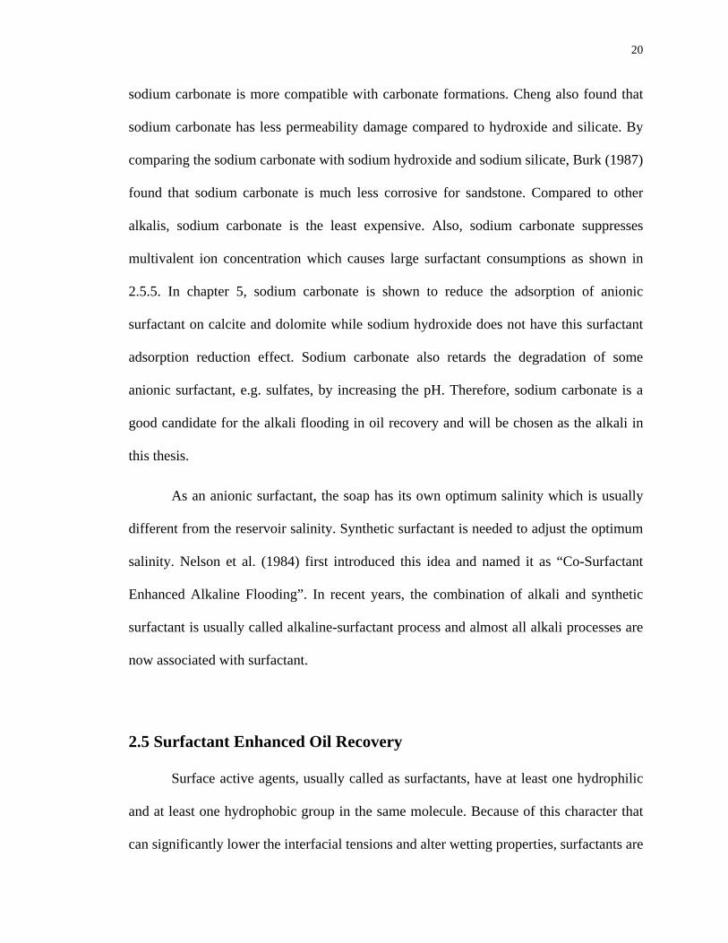
Figure 2.7 schematic plots of microemulsions

(a) oil-in-water (o/w) microemulsions (Miller and Neogi, 1985)

(b) water-in-oil (w/o) microemulsions (Miller and Neogi, 1985)

(c) bicontinuous microemulsions (Scriven, 1976)

Macroemulsions, sometimes just called emulsions, are thermodynamically

unstable to microemulsions. The suspended droplets will eventually agglomerate and/or

coalesce, and the dispersed phase will separate. Macroemulsion droplet sizes are typically

much larger, one micron or more, resulting in a cloudy or milky dispersion. The nature of

a macroemulsion may depend on the order of mixing of the ingredients and the amount of

energy put into the mixing process.

2.5.3 Phase Behavior of Microemulsions

The phase behavior of microemulsions is very important to enhanced oil recovery

because it can be used as an indicator of ultra-low interfacial tension. Phase behavior

screening helps to quickly evaluate favorable surfactant formulations. Winsor (1954) first

described the phase behavior of microemulsions for surfactant, oil and brine system. The

phase behavior of a microemulsion system is a function of types and concentration of

surfactants, cosurfactants, oil, brine, alcohol, temperature, etc. In a particular

27

microemulsion system containing an ionic surfactant, the concentration of the electrolyte,

or the salinity, will be an important impact factor on phase behavior.

Figure 2.8 Microemulsion ternary phase diagram for different salinity

(Adapted from Healy et al, 1976)

Ternary phase diagrams, a convenient tool for describing the microemulsion

phase behavior (Healy, et al., 1976; Nelson and Pope, 1978), exhibit how salinity changes

the phase behavior. With varying salinity, the phase behavior of microemulsions can be

divided into three classes, lower-phase microemulsion, upper phase microemulsion and

28

middle phase microemulsion. Figure 2.8 illustrates the relationship between salinity and

phase behavior.

The main mechanism by which salinity affects microemulsion phase behavior

with ionic surfactants is the electrostatic forces, for instance those between charged

surfactant head groups in surfactant films covering the surfaces of microemulsion drops.

These forces will spontaneously change the curvature of the drops, which, in turn,

determines the type and solubilization capacity of the microemulsions. At low salinities,

the microemulsion is an oil-in-water microemulsion that coexists with nearly pure excess

oil. Since the density of this kind of microemulsion is larger than the oil, it is below the

oil so that this microemulsion is called “lower phase” microemulsion. Also, it is named

as Winsor type I, or type II(-) because the slope of the tie lines of lower phase

microemulsion is negative. In this microemulsion, the radius of microemulsion drop will

become larger and solubilization of oil will be enhanced with increase of salinity, i.e., the

repulsion between the charged head groups decreases.

When the salinities are very high, the electrostatic forces from the electrolytes

will change the sign of the drop curvature so that the water-in-oil microemulsion forms. It

is called an “upper phase” microemulsion because the microemulsion is lighter that the

water and above the water phase. The upper phase microemulsion is also named type II

(+) or Winsor type II. Opposite to the “lower phase” microemulsion, the drop size and

drop radius decrease with increasing salinity.

At intermediate salinities, three phases are present. A microemulsion is formed in

equilibrium with both excess oil and brine. This microemulsion, which is called “middle

phase” microemulsion, contains almost all the surfactants in the system. Similarly,

29

middle phase microemulsion is also named type III, or Winsor type III. This type of

microemulsion is of great importance in enhanced oil recovery because of its ultra-low

interfacial tension that we will mention in the next section. The middle phase structure is

complicated and has attracted many researchers. Scriven (1976) postulated that the

middle phase has a bicontinuous structures (see, Figure 2.7 (c)). Theoretical models and

some experimental observations were made to develop the bicontinuous microemulsion

models (Burauer S. et al., 2003). The bicontinuous structure is similar to a consolidated

porous medium where both the solid and pore space are continuous, although, of course

much smaller. Since both the oleic phase and aqueous phase are continuous, the

interfacial tensions between the middle phase and either excess brine or excess oil are

very low.

To visualize the microemulsion change, figure 2.9 shows a typical example of

how phase behavior changes with salinity.

NaCl concentration increases

System containing a petroleum sulfonate surfactant, a short-chain alcohol, oil and brine

NaCl concentration increases

System containing a petroleum sulfonate surfactant, a short-chain alcohol, oil and brine

Figure 2.9 Effect of salinity on microemulsion phase behavior (Miller and Neogi, 1985)

30

2.5.4 Phase Behavior and Interfacial Tension

Healy and Reed (1974, 1976, and 1977) first developed an empirical correlation

between the microemulsion phase behavior and the interfacial tension as figure 2.10

illustrates. Solubilization ratios were introduced to describe the microemulsion phase

behavior.

I II

Figure 2.10 Interfacial tension and solubilization parameter versus salinity

(Reed and Healy, 1977)

Figure 2.10 represents the corresponding behavior of the solubilization parameters

and IFT with different salinity. In the upper part this figure, σmo is the IFT between the

microemulsion and the excess oil phase, and σmw is the IFT between the microemulsion

and water phase. In type I region, moσ is high and mwσ does not exist; while in type II

region, moσ does not exist and mwσ is high. In type III region, moσ and mwσ are of the

31

similar magnitude with very low value. The salinity where the two tensions are equal is

called the optimum salinity, which is one of the most significant quantities in the

surfactant flooding process. As discussed in 2.3, if interfacial tension is small, capillary

number will be large enough to let the residual oil saturation goes to zero. This is one of

the main mechanisms for enhanced oil recovery with surfactants. Healy and Reed (1977)

also confirmed that the optimum salinity was the same as the salinity for maximum oil

recovery by core flooding experiments. Clearly, one of the goals of surfactant flooding in

enhanced oil recovery is to have the surfactant at the displacement front near optimum

conditions.

The solubilization parameter Vo/Vs is defined as the volumetric ratio of

solubilized oil to surfactant, and Vw/Vs is water to surfactant in the microemulsion phase.

In the lower part of figure 2.10, Vo/Vs increases with salinity, while Vw/Vs decreases

with salinity. At optimum salinity, the amount of oil and brine solubilized in the

surfactant phase are approximately equal. This is also another definition of optimum

salinity. Also equal contact angles could be found at the optimum salinity (Reed and

Healy, 1984).

Huh (1979) derived a theoretical relationship between solubilization ratio and IFT.

Huh’s theory predicts that the IFT varies with the inverse square of the solubilization

ratio as 2.17. In Huh’s equation, C=0.3 is a good approximation for most crude oils and

microemulsions. Glinsmann (1979) experimentally validated this relationship. In chapter

4, IFT experimental results substantiate this equation.

( )2/ si VVC

=σ i = water or oil (2.17)

32

As shown in chapter 4, the IFT measurement between microemulsion and water

and/or crude oil is time consuming and more difficult than the phase behavior

observations. Sometimes, it is almost impossible to measure the IFT between some crude

oil and its lower phase microemulsion. By using phase behavior observation and

measurements of the solubilization ratios, it is much simpler and faster to estimate the

IFT of the oil/water/microemulsion system, especially for the surfactant screening. Of

course, it is always worth verifying the IFT measurement if a good formulation is

identified by phase behavior.

2.5.5 Surfactant Retention

To have a successful commercial application of surfactant process, the surfactant

retention should be minimized. Surfactants may be retained through these mechanisms:

adsorption, precipitation, ion exchange and phase trapping (Green and Willhite, 1998).

2.5.5.1 Surfactant adsorption on mineral surface

Due to the different mineralogy, most solid surfaces, including reservoir rocks,

are charged. While silica may be negatively charged, calcite, dolomite and clay may have

positive charge on their surfaces at neutral pH. The most important cause of ionic

surfactants adsorbing onto a solid is often the electrical interaction between the charged

solid surface and surfactant ions, which can be explained by electrical double layer theory

(Wesson and Harwell, 2000). Sometimes, surfactant adsorption is presented as the

amount of surfactant adsorbed per unit solid weight versus equilibrium surfactant

33

concentration. It is better to use the amount of surfactant adsorbed per unit of solid

surface area to describe the surfactant adsorption. Lake (1989) suggested that the

Langmuir-type isotherm of adsorption could describe surfactant adsorption. The

surfactant adsorption will not increase when critical micelle concentration (CMC) of the

surfactant is reached. The adsorption model of Wesson and Harwell (2000) also supports

this Langmuir adsorption except their model is more subtle when the surfactant

concentration is less than CMC.

The amount of adsorbed surfactant depends on the surfactant character (the

surfactant type, the structure of the chain), the rock properties (surface charge), pH,

potential determining ion in solution and salinity. The pH may alter the surface charge to

change the adsorption amount; the salinity may change the electrical potential of surface

sites for the adsorption. For example, Glover (1978) showed that retention increased

linearly with salinity at low salt concentrations and departed from linearity with higher

retentions above a critical salinity. Hirasaki and Zhang (2002) found that the potential

determining ions (CO32-) can change the surface charge and reduce the anionic surfactant

adsorption on calcite. Grigg and Bai (2005) found that a decreasing order of a surfactant

(CD1045) adsorption density (mg/g) onto the five powdered minerals is: montmorillonite,

dolomite, kaolinite, silica and calcite. However, the surface area of their mineral was not

reported. Chapter 5 will discuss surfactant adsorption further.

2.5.5.2 Surfactant Precipitation

In hard brines, the presence of divalent cations causes surfactant precipitation as

equation 2.18 shows.

34

↓→+ +−2

22 MRMR (2.18)

where R- is the anionic surfactant;

MR2 is the surfactant-divalent cation complex that has a low solubility in brine.

This reaction leads to retention. Factors that influence the precipitation of anionic

surfactants include cation valence, salt concentration, surfactant concentration, alcohol

concentration, temperature, etc (Green and Willhite, 1998). When oil is present, it can

compete for surfactant; that is, addition of oil can reduce (in some cases completely

eliminate) surfactant precipitation. Also the precipitate must compete with the micelles

for the surfactants (Somasundaran et al., 1979). Celik (1982) proved that surfactant

precipitation increases with surfactant concentration at low concentration. But it will re-

dissolve because the micelles will take up multivalent ions, causing redissolution of the

precipitation. Addition of alcohol increases the solubility of a surfactant when the

alcohol/surfactant ratio is sufficiently high (Green and Willhite, 1998). Also, the

ethoxylate (EO) and propoxylate (PO) groups will help the surfactant to have tolerance to

divalent cations typically present in reservoir brines. In this thesis, the surfactants

considered have EO and PO groups, so that they have high tolerance to divalent cations.

Thus, precipitation will not be discussed further in this thesis.

2.5.5.3 Phase Trapping

This form of retention is strongly affected by the phase behavior. Surfactants may

exist in the oil phase, and oil phase could be trapped as residual oil (Green and Willhite,

1998). Phase trapping can contribute significantly to surfactant retention and should

35

always be avoided. Glover et al. (1979) found that the onset of phase trapping with a

surfactant-flooding process generally occurred at higher salt concentrations because it

would form upper-phase microemulsion so that the surfactant would be trapped in the

residual oil. Divalent cations are shown to influence microemulsion phase behavior

strongly so that the phase trapping may occur at low divalent ion concentration compared

to mono-valent ion concentration.

At lower hardness level, the multivalent cation will react with the anionic

surfactant to form a monovalent cation that can chemically exchange with cations

originally bound to the reservoir clays (Hill and Lake, 1978) as (2.19) and (2.20).

++− →+ MRMR 2 (2.19)

++ +−→+− NaClayMRMRClayNa (2.20)

This form of retention is reversible with both M2+ and surfactant concentration.

Other researchers (Hirasaki, 1982; Hirasaki and Lawson, 1986) found that ion exchange

of the cations (Na+, Ca2+) with both the clays and the surfactant micelles is much more

important for the surfactant retention. A system in which the preflood, slug, and drive

have the same sodium and calcium injected concentration can have a significant increase

in the calcium concentration in the surfactant bank and a significant decrease in calcium

concentration in the drive because of ion exchange. Thus, the salinity of the surfactant

flood will be over optimum salinity and form upper-phase microemulsion, i.e. the

surfactant will reside in the oil phase and does not move with the flooding front.

Krumrine (1982) proposed that the addition of alkali would reduce the concentration of

36

hardness ions that may cause surfactant retention. Therefore, ASP will have little

surfactant retention due to ion exchange.

A trapped, upper-phase microemulsion may be remobilized by flushing with

sufficiently lower salinity to cause an in-situ change to a middle- or lower-phase micro-

emulsion (Hirasaki et al., 1983). As shown in this thesis, ASP process has a lower-phase

region behind the surfactant front, i.e. the surfactant is partition into lower-phase and

remobilized again. Thus, ASP process minimizes the retention by phase trapping with the

lower-phase microemulsion region after surfactant front.

2.5.6 Co-solvents in surfactant process

Co-solvents, normally low molecular weight alcohols, are frequently used in

surfactant process. In many surfactant systems, especially at high surfactant or low

temperature conditions, high viscosity liquid crystals, emulsions and gels are observed

(Healy and Reed 1974; Miller & Neogi, 1985). These phases with large viscosities will

be trapped in the porous medium so that the surfactants can not propagate in reservoirs.

The most important reason for using alcohols is to inhibit the formation of those high

viscosity phases (Sanz and Pope, 1995). There are still some other reasons to use alcohol

in surfactant process. The optimum salinity can be adjusted by alcohol. The type and

concentration of alcohols change the optimum salinities (Salter, 1978; Lelanne-Cassou et

al., 1983). Trushenski (1977) claimed that alcohol can eliminate the polymer-surfactant

incompatibility. The presence of alcohol helps to reduce the emulsion coalesce time(Sanz

and Pope, 1995).

37

However, introducing alcohols into surfactant process also has significant

negative effects. Alcohols always raise the minimum interfacial tension (IFT) as well as

decrease the solubilization ratios. This IFT incremental effect by alcohol is detrimental to

oil recovery because IFT reduction is the main mechanism for surfactant enhanced oil

recovery. Foam is unstable when alcohol is present (Li, 2006). It is difficult to use foam

as mobility control where there is alcohol. Adding alcohol also increases the chemical

cost and makes the surfactant process more complicated because of this additional

component. Because of these harmful properties, it is better to have an alcohol-free

formulation for oil recovery. Sanz and Pope (1995) found that the alcohol could be

eliminated in several conditions. This thesis uses the blend of branched alcohol propoxy

sulfates and internal olefin sulfonate to avoid the need for alcohol. Although alcohol will

not be further discussed in this thesis, we still should remember that alcohols are quite

effective to eliminate viscous phases.

2.5.7 Cationic Surfactant Flooding

While anionic surfactants are the most used surfactants in oil recovery processes,

other surfactants, especially the cationic surfactants, have been considered (Austad and

Milter, 1997; Austad et al., 1998; Standnes and Austad, 2000; Standnes et al., 2002,

2003, Strand, 2004). Unlike anionic surfactant flooding, the main mechanism of cationic

surfactant flooding is wettability alteration. The mechanism of wettability alteration is the

formation of ion-pairs between the positively charged surfactant monomers and

negatively charged adsorbed material, mainly carboxylic groups. The resulting desorption

makes the rock surface more water-wet, and water will spontaneously imbibe into the

38

matrix due to capillary effect. The desorbed material may exist in the micelles, or in the

oil phase in the form of ion-pairs. Standnes and Austad (2000) also found that cationic

surfactant adsorption is low in low-permeable chalk.

2.6 Mobility Control in Enhanced Oil Recovery

The purpose of mobility control is to change the mobility ratio to a favorable

number so that the injected fluid will not bypass the displaced fluid, i.e. crude oil in

reservoir. Because it is not economically practical to change the properties of the crude

oil or the permeability of the reservoir, most mobility control methods change the

properties of injected fluid. The commonly used mobility control agent is polymer

because it can significantly increase the apparent viscosity of the injected fluid. Foam is

also a good mobility control method with water, surfactant and gas. Because low

surfactant concentrations are used and much of the injected material is gas, the cost of

chemical for foam can be much less than the polymer. However, foam is more

complicated than the polymer applications and the mechanism of foam transport in

porous media is still not fully understood (Yan, 2006). Water-alternating-gas (WAG) is

also used to control the mobility in some gas enhanced oil recovery process.

2.6.1 Polymer process

Addition of polymer will increase the viscosity of aqueous phase, so that the

mobility of aqueous phase decreases. Thus the mobility ratio will be lower with polymer.

Unlike the surfactant, the presence of polymer will not decrease residual oil saturation

39

with a few exceptions (Wang et al., 2000). But it will greatly increase sweep efficiency.

If the waterflooding mobility ratio is high, the reservoir heterogeneity is serious, or

combination of these two happens, polymer flooding will be useful (Lake 1989). Yang et

al. (2006) found that an incremental recovery over water flooding of more than 20%

OOIP can be obtained by injection of high molecular weight, high concentration polymer

solution in Daqing field.

When polymer is used in surfactant flooding, it can also provide the mobility

control at the low IFT front. Otherwise, the front is not stable and will finger and

dissipate. Falls et al. (1992) tested an alkaline-surfactant process without using polymer

within the White Castle Field, Louisiana. Although this process exhibited a displacement

efficiency of virtually 100%, it recovered only 38% of the waterflooding residual oil in

the reservoir as true tertiary oil due to the absence of mobility control. This thesis shows

that maintaining the mobility is also very important for ASP flooding. Even when the

residual oil saturation is zero, the oil recovery will be small without a favorable mobility

ratio.

Two types polymers, polyacrylamide and polysaccharide, are commonly used in

enhanced oil recovery (Sorbie, 1991). Polyacrylamides used in polymer EOR processes,

normally are partially hydrolyzed polyacrylamides (HPAM). Thus, the HPAM is

negatively charged, as is the anionic surfactant. Shupe (1981) tested the effect of pH,

dissolved oxygen, salinity and hardness on HPAM polymer stability. HPAM has been

used in about 95% of the reported polymer tests (Lake, 1989). The commonly used

polysaccharide is xanthan gum, which is a bacterial polysaccharide. Compared to HPAM,

xanthan gum has a more rigid structure than HPAM and relatively nonionic. These

40

properties make it relatively insensitive to salinity and hardness. However, it is

susceptible to bacterial degradation after it has been injected into the field. In this thesis,

only HPAM is used as the polymer.

2.6.2 Foam process

Foam is a two-phase system in which a relatively large volume of gas is dispersed

in a small volume of liquid (Patton et al., 1983). In porous media, the liquid phase of

foam is continuous and at least some part of the gas phase of foam is made discontinuous

by thin liquid films (Hirasaki, 1989). The presence of discontinuous gas in foam not only

reduces the gas mobility but also reduces the liquid saturation and relative permeability

and hence raises liquid phase apparent viscosity. One of the main reason that apparent

viscosity of gas phase increases is that an extra force is required to push thin liquid films

(lamellae) through pore throats of porous media. Also the viscous shear stresses in the

thin films between the pore walls of porous media and gas interface increases the

apparent viscosity (Nguyen et al., 2000). Foam can be stabilized by some surfactants. If

foam can successfully replace the polymer as the mobility control agent, it may reduce

the chemical cost for the surfactant process (Yan, 2006).

2.7 Alkaline-Surfactant-Polymer Enhanced Oil Recovery

Currently, alkaline-surfactant-polymer (ASP) is considered as the most promising

chemical method in enhanced oil recovery because it integrates the advantages of alkali,

surfactant and polymer. In recent years, there have been several field pilot tests using

41

ASP in USA (Pitts et al., 2006), India (Pratap and Gauma, 2004) and China (Wang et al.,

1997; Qiao et al., 2000; Li et al., 2003; Yang 2003; Chang et al., 2006). However, the

mechanisms of the alkaline-surfactant flooding are still not fully understood. Most

investigators agree that the key issues for the alkaline-surfactant flooding are IFT

reduction at low surfactant concentration, wettability alteration, low adsorption of

surfactant by alkali, and mobility control.

Like surfactant process, IFT reduction is considered as one of the most important

factors in alkaline-surfactant flooding (Falls et al., 1992; Arihara, et al., 1999). Krumrine

et al. (1982) found that low IFT could be achieved with several alkaline chemicals and

dilute surfactant systems. With the addition of a small amount of surfactant to the

alkaline solution, the interfacial tension can become lower than with either surfactant or

alkali alone (Schuler et al., 1989). Rudin and Wasan (1992) claimed that the organic acid

amount in the oil has significant effect on the IFT reduction of alkaline-surfactant-oil

system. They found that at low acid concentrations, the addition of an alkali to the added

surfactant solution would only make interfacial tension increase. But at medium to high

acid concentrations, the addition of an alkali can produce ultralow interfacial tension.

They also observed that the addition of alcohol (isobutanol) could shift the minimum in

IFT and reduce the time needed to achieve equilibrium interfacial tension. Nasr-El-Din

and Taylor (1992; 1996) found the alkali-surfactant mass ratio changes the time to

achieve minimum IFT by using dynamic IFT measurement. Hirasaki and Zhang (2003)

found that there were optimum conditions for the IFT reduction by changing the

concentration of alkali and surfactants. Seethepalli et al. (2004) identified that some

42

anionic surfactants could lower the IFT with a West Texas crude oil to very low values

(<10-2 mN/m).

Many other researchers also found that the ultra-low IFT existed in the alkaline-

surfactant systems and would be the main reason for enhanced oil recovery (Nelson et al.,

1984; Martin et al., 1985; Olsen et al., 1990; French and Burchfield, 1990; Baviere et al.,

1995; Gao et al., 1995, 1996; Al-Hashim et al., 1996; Arihara et al., 1999; Vargo et al.,

2000; Hirasaki and Zhang, 2003, Zhang et al. 2006). One of the biggest differences

between ASP process and surfactant process is that ASP has two surfactants, synthetic

surfactant that is injected and the natural soap created by the alkali in situ. Due to the

different hydrophilic properties, they have different optimum salinities. This is one of the

crucial factors of the process. This thesis will illustrate this relationship and try to use

this characteristic to optimize the ASP process.

In addition to low interfacial tension, wettability alteration is also considered as

an important factor for ASP recovery mechanism. As discussed section 2.4, the addition

of alkali may result in wettability alteration. ASP process inherits this effect of alkaline

flooding. Recent studies showed that alkali with dilute surfactant solution can change the

wettability. Some successful imbibition experiments substantiated the results (Xie and

Morrow, 2001; Hirasaki, and Zhang, 2003; Adibhatla and Mohanty, 2006). In this thesis,

the wettability alteration will not be further discussed. We still should keep in mind that

wettability alteration is very important for alkaline-surfactant EOR, especially for the

fractured, oil-wet reservoir which spontaneous imbibition might be more suitable than

flooding process.

43

As discussed in 2.5.5, the presence of alkali also reduces the consumption of

surfactant. It has long been recognized that alkali can reduce the surfactant adsorption.

Many experimental results showed mitigation of the surfactant adsorption by alkali.

Polymer in ASP will act as the mobility control agent as shown. With the synergetic

effect of alkali, surfactant and polymer, ASP process shows a great potential for

enhanced oil recovery.

2.8 Numerical Simulation

Numerical simulation is very important to evaluate a process before the actual

application because it will save time, cost and effort. And the numbers and complexities

of flooding experiments can be minimized with numerical simulation. Thus, it is

necessary to build a model to simulate the ASP process besides carrying out the

experiments. With a good ASP numerical simulation, it will help the researchers to

understand the characteristics of the ASP process.

Pope and Nelson (1978) developed a 1-D numerical simulator for surfactant

enhanced oil recovery. Now it has been extended to include other chemical processes and

to 3-D as UTCHEM (Delshad et al., 2002; Zerpa et al., 2004; John et al., 2005; Anderson

et al., 2006). There are several commercial reservoir simulators, such as ECLIPSE by

Schlumberger, VIP® and Nexus® by Halliburton. Several major oil and gas companies

develop so called "in-house" packages for themselves, such as CHEARS by Chevron,

Empower by ExxonMobil. However, most simulators do not include natural soap which

is one of the most important factors in ASP. UTCHEM models the natural soap as an

44

additional surfactant (Delshad et al., 1998). But it does not distinguish the natural soap

from the injected synthetic surfactant. The simulation in this thesis includes soap and its

effect on the optimum salinity for ASP. Although it is a simple 1-D model so that it is

faster and will not have many numerical convergence problems, it illustrates the

characteristics of the ASP process and helps us to understand and optimize the process.

45

Chapter 3

Phase Behaviors of Alkali-Surfactant System

This chapter presents the phase behavior experiments, also known as emulsion

screening test, conducted for this research. The objective of phase behavior studies is to

determine the optimum salinity by observing the alkali-surfactant-crude oil samples.

Different oil samples are tested to illuminate the alkaline-surfactant phase behaviors.

3.1 Materials

3.1.1 Surfactant Selection

The surfactants used in the phase behavior experiments are the blends of 4:1

weight ratio (active material) of Neodol 67-7PO sulfate (N67) from Stepan and C15-18

internal olefin sulfonate (IOS) from Shell chemical. In this thesis, this blend is also called

NI Blend.

Sulfates are selected because of the low cost of ethoxylated and propoxylated

sulfates compared to the corresponding sulfonates. The ethoxy (EO) and propoxy (PO)

groups give the possibility to tailor the surfactant molecules for oil recovery (Osterloh,

and Jante, 1992; Aoudia et al., 1995; Wu et al., 2005; Levitt et al., 2006). The EO and PO

groups can also raise the tolerance to divalent ions (Osterloh, and Jante, 1992). However,

sulfate will hydrolyze at high temperature (> 60 °C) with the presence of an ester linkage

(Aoudia et al., 1995). In this thesis, all the experiments are at room temperature so that

46

sulfates can be used. The hydrophobe for this Neodol 67-7PO sulfate is a 16 to 17 chain

with an average of 1.5 methyl groups randomly positioned (Annual DOE Report, 2006).

The branched chain is introduced to decrease the formation of ordered structure, e.g.

liquid crystals. An approximate structure of a C16-17 7PO sulfate molecule generated by a

space filling, free-energy minimizing model is shown in Figure 3.1 (a).

Sulfonates have been considered and tested for surfactant EOR process for several

decades. Unlike the sulfates, sulfonates are thermally stable at much higher temperatures

(Salter, 1986). The sulfonate used in this thesis is C15-18 internal olefin sulfonate (IOS).

The internal olefin will have an overall size of C15 to C18 and a range of internal,

double-bond positions such that sulfonation with SO32- will produce a variety of products.

This is also expected to minimize the formation of ordered structures such as liquid

crystals and gels (Annual DOE Report, 2004). The hydroxyl alkane sulfonate form of a

C15-18 IOS is shown in Figure 3.1 (b).

Figure 3.1 Possible structures of (a) C16-17-(PO)7-SO4 (b) C15-18 Internal Olefin Sulfonate (IOS) (Annual DOE Report, 2006)

47

The NI blend is selected because it exhibited the most promising performance

with Yates and Midland Farm oils (Annual DOE Report, 2006; Zhang et al., 2006; Levitt

et al., 2006). This blend has good solubility behavior without forming liquid crystals or

gels. Another reason to choose the NI blend is that NI blend can be injected as a single

phase solution at ambient temperature at high salinities as shown in figure 3.2. It is very

important to keep the ASP solution as one phase to avoid highly viscous phases. Figure

3.2 shows that NI blend has much higher salt tolerance than IOS or N67 by itself. Liu et

al. (2006) also reported that the surfactant blend will increase the calcium tolerance for

surfactant.

Phase boundary

Precipitate of surf.

Clear solution2 clear phases

Cloudy solution

3 % surfactant + 1% Na2CO3 , 1 week

%N

aCl

0123456789

10

IOS-15/18 N67-7PO S1:1 4:1

N67-7PO S:IOS-15/18 (w/w)

9:1

1-Phase Region

**

**

Multi-Phase Region

Phase boundary

Precipitate of surf.

Clear solution2 clear phases

Cloudy solution

3 % surfactant + 1% Na2CO3 , 1 week

%N

aCl

0123456789

10

IOS-15/18 N67-7PO S1:1 4:1

N67-7PO S:IOS-15/18 (w/w)

9:1

1-Phase Region

**

**

Multi-Phase Region

Figure 3.2 Effect of added NaCl on phase behavior of 3 wt% solutions of N67/IOS mixtures containing 1 wt% Na2CO3. (Liu et al., 2006)

48

3.1.2 Crude Oils

Yates crude (MY) oil and PBB crude oil have been extensively investigated in

this chapter. MY represents the crude oil with low acid number (0.2 mg KOH/gram oil by

Fan and Buckley, 2006) and moderate viscosity (19 cp at ambient temperature); PBB is

the oil with much higher acid number (4 mg KOH/gram oil) and high viscosity (266 cp at

ambient temperature). A few samples with Shell White Castle Q-sand (SWCQ) oil (1.5

mg KOH/gram oil and 2.8 cp) and synthetic oils (octane, decane, dodecane) were also

tested. The synthetic oils are from Sigma-Aldrich.

3.1.3 Other Chemicals

Deionized (DI) water: Deionized (DI) water with conductivity of 4-7 μS/cm was

used for all experimental solutions.

Sodium carbonate: Sodium carbonate from Fisher, is ≥99.8% pure with less than

0.005% calcium. Sometimes, the sodium carbonate solution has to be filtered because of

a very small amount of precipitation.

Sodium chloride: Sodium chloride, which adjusts the electrolyte strength, is a

Fisher product. It is enzyme grade with ≥99.9% sodium chloride.

Sodium hydroxide: Sodium hydroxide, which is used in soap extraction, is also a

Fisher product with 98.5% sodium hydroxide.

Isopropyl alcohol: Isopropyl alcohol (IPA), which is used in soap extraction, is a

Fisher product with ≥99% IPA.

49

3.2 Soap Extraction for crude oils

As discussed in Chapter 2, natural soap, which is an anionic surfactant, will be

generated by the saponification of the acidic components in the crude oil with alkali.

Thus, the soap amount, or the natural surfactant concentration, is a very important value

for phase behavior study. Usually, acid number determined by non-aqueous phase

titration (Fan and Buckley, 2006) is used to estimate the soap amount (Zhang & Hirasaki,

2006). However, short chain acids, which also react with alkali, may not behave like

surfactant because they are too hydrophilic. Also phenolics and porphyrins in crude oil

will consume alkali and will not change the interfacial properties as much as surfactant.

Asphaltenes and/or resins may have carboxylate functional groups but not be extracted

into the aqueous phase. Total acid number determined by non-aqueous phase titration

could not distinguish the acids that can generate natural soap and those that can consume

alkali without producing surfactant. Therefore, another method that can obtain the soap

amount is introduced.

Since the anionic surfactant can be accurately determined by potentiometric

titration (See Appendix A) with Benzethonium Chloride (hyamine 1622), it is reasonable

to use this method to find the natural soap amount. Since this potentiometric titration is

for aqueous phase, the soap should be extracted into aqueous phase as the first step. As an

anionic surfactant, the natural soap may stay in the oleic phase and form upper-phase

microemulsion when the electrolyte strength is high. To extract the soap into aqueous

phase, NaOH was used to keep the pH high with low electrolyte strength. Also isopropyl

alcohol was added to make the system hydrophilic so that soap will partition into aqueous

phase. The extraction procedure is shown as below:

50

1. Mix crude oil, 0.1 M NaOH solution and isopropyl alcohol (IPA) together. The

weight ratio is 1 (oil): 3 (NaOH): 0.44 (IPA). This ratio was chosen because it assures

the NaOH is enough to react with the acid in the oil and still keep pH around 13.

2. Shake the sample well by hand for 1 or 2 minutes and keep on shaking sample by a

rotating shaker for 24 hours.

3. Settle the sample until the water oil interface does not change.

4. Sample the aqueous phase and determine the aqueous phase surfactant concentration

by potentiometric titration with hyamine. (for PBB, the sample is never settled, and

entire emulsion was used for titration)

5. Use mass balance to calculate the acid number.

0.34 0.16 0.37* 0.75 2.2** 4.8

Midland Farm Minas Mars Yates White Castle PBB

~0 0.02 0.10 0.14 0.65 1.25

3 grams oil with 9 grams 0.1 M NaOH and ~1.3 gram IPA

Acid Number (mg KOH/gram oil) by soap extraction

Acid numbers (mg KOH/gram oil) by non-aqueous phase titration* (Yang, 2000) **(Falls et al., 1992)

OMF CM Mars Yellow MY SWCQ PBB

Figure 3.3 Soap extraction behaviors and acid numbers by soap extraction and

non-aqueous phase titration.

51

Figure 3.3 shows the photos of soap extraction and compares the acid number

determined by soap extraction and non-aqueous phase titration. Six different crude oils

were tested. Since those acids that can not generate soap will not detected by the

potentiometric titration, the acid numbers obtained by the soap extraction are less than the

acid numbers determined by non-aqueous phase titration as expected. There is no general

ratio between those two acid numbers, i.e., the natural soap amount of an oil can not be

determined just by non-aqueous phase titration. Oils with high acid number by non-

aqueous phase titration usually have high soap content. But it is not always true. For

example, the higher acid number of Midland Farm by non-aqueous phase titration is 0.34

mg KOH/ g, which is higher than Minas oil (0.16 mg KOH/g) and close to Mars (0.37 mg

KOH/g). But no soap can be found by soap extraction for Midland Farm, while the Minas

is 0.02 mg KOH/g and Mars is 0.10 mg KOH/g by the soap extraction. The other

interesting observation is that the color of the aqueous phase indicates how much soap

has been extracted. Darker aqueous phase indicates higher extracted soap. This is

reasonable because naphthenic acids are colored and also higher soap concentration will

help dissolve more oil into the aqueous phase so that the aqueous phase will be darker.

3.3 Phase behavior Experimental Procedure

The concentrated stock solutions of surfactant, sodium carbonate and sodium

chloride were prepared before mixing them together. All solutions were made by weight

percentage. By mixing the stock solutions and DI water in different ratios, the solutions

over a range of salinities were made. The solutions should be made in this order:

52

1. Sodium chloride and sodium carbonate stock(s)

2. De-ionized water

3. Surfactant stock(s) which has been mixed as NI blend

This order was chosen because the surfactant solution will precipitate or have

phase separation problems at high salinity. The tips of 5 ml glass pipettes from Fisher

Brand® or similar pipettes were sealed by acetylene and oxygen flame with VICTOR®

torch. Then, the surfactant solutions and crude oils were mixed at a specific Water Oil

Ratio (WOR) into these pipettes. After the mixing procedure, the other ends of the

pipettes were sealed so that water and volatiles in crude oil will stay in the samples.

Afterwards, the samples were shaken well by hand for 1 or 2 minutes and put on a

rotating shaker for 24 hours to provide adequate mixing. Finally, they were arranged on

the racks to settle in an upright position. Photos were taken to record the phase behaviors

which would be used to calculate the solubilization ratios. The oil water interface changes

with settling time. The equilibrium phase behavior was usually achieved after 7 days

because no further changes were observed in the interface positions, i.e. phase volumes.

In the next section about phase behavior results, all the phase behavior results are

equilibrium.

3.4 Phase behavior Results

3.4.1 Phase Behavior of PBB and NI Blend

Fig. 3.4 (b) illustrates variation of phase behavior with NaCl concentration for

alcohol-free solutions containing 0.2 wt% (active) NI blend and 1 wt% Na2CO3 mixed

53

with PBB crude oil at a water-to-oil (WOR) ratio of 24 and stored at ambient temperature

for 40 days. Hereafter, all the surfactant, sodium carbonate and sodium chloride

concentrations are based on aqueous solutions. The concentration of Na2CO3 was chosen

as 1% because this concentration will assure the low surfactant adsorption even with the

consumption of surfactant by acid in crude oil as shown in Chapter 5. The photos for

those samples were taken after 40 days because such a long time assures that the

equilibrium is achieved. In fact, no further changes for the interfaces of those samples

were observed after 10 days. At 4.8 % NaCl, it is lower phase microemulsion (Winsor I)

because the aqueous phase volume is greater than its initial volume. As discussed in

Chapter 2, the incremental volume in the lower phase is due to the solubilization of oil by

the surfactant in aqueous phase. When the salinity is at 5.2% NaCl, it is upper phase

microemulsion (Winsor II) because the swelled oleic phase indicates that surfactant is in

oleic phase and solubilizes water. It is difficult to observe the classical Winsor type III

region for crude oil system with such a low surfactant concentration (0.2%). Phase

behavior with crude oil and low surfactant concentration often changes from Winsor I to

Winsor II directly. Therefore, the optimum salinity is located as the salinity between the

highest Winsor I salinity and the lowest Winsor II salinity. Therefore, the optimum

salinity of Figure 3.4 (b) is around 5.0% NaCl. Optimum salinities for other samples were

similarly determined as shown in figure 3.4(a) and 3.4(c).

Figure 3.4 also represents that optimum salinity is a function of both surfactant

concentration and WOR for PBB and NI blend. Fig 3.4 (a) is around 3.2 % NaCl at 0.05

% surfactant concentration with all the other conditions identical to Figure 3.4 (b). And

54

the optimum salinity is between 2.4 and 3.0% with WOR at 3 with all the other

conditions identical to Figure 3.4 (b).

0.2%24,

0.2%24,

X= 2.0 2.2 2.4 2.6 2.8 3.0 3.4 % X= 1.0 1.6 2.0 2.4 3.0 3.2 %X= 4.0 4.4 4.8 5.0 5.6 6.0 %

NI blend,WOR=

1% Na2CO3/X% NaCl

NI blend,WOR=3,

1% Na2CO3/X% NaCl

0.05% NI blend,WOR=

1% Na2CO3/X% NaCl

Optimum Salinity Figure 3.4 Phase behavior is a function of WOR and surfactant concentration for

PBB and NI blend at ambient temperature.

The optimum salinities for other surfactant concentrations and WORs are also

plotted in Figure 3.5. The point with 0% surfactant concentration in figure 3.5 indicates

that the optimum salinity for soap is around 0.8% NaCl. And optimum salinity for PBB

and NI blend without any Na2CO3 is around 7.5 % NaCl. It is consistent with figure 3.5

that the optimum salinity increases to above 6% NaCl with presence of 1% Na2CO3 when

both surfactant concentration and WOR are high. From figure 3.5, the optimum salinity

can be increased by raising either the surfactant concentration or WOR. The similarity

between raising the surfactant concentration and increasing WOR is that the ratio of

natural soap to synthetic surfactant deceases. It is reasonable that the soap to surfactant

55

ratio is the parameter that determines the optimum salinity. Figure 3.6 shows that the

dependence of optimum salinity on surfactant concentration and WOR can be correlated

with natural soap/synthetic surfactant mole ratio. The three curves with different WORs

in figure 3.4 collapse into one curve as shown in figure 3.5. The soap amount is based on

the soap extraction. When soap to surfactant ratio is low, i.e., surfactant is dominant, the

optimum salinity goes to the optimum salinity of the surfactant (~6.5% NaCl + 1%

Na2CO3); while when the ratio is high, i.e., soap is dominant, the optimum salinity is

close to the optimum salinity of soap (~0.8% NaCl + 1% Na2CO3). The fact that optimum

salinity is a function only of the soap/surfactant ratio is a very important property for the

alkali surfactant crude oil system. And this property is very beneficial to design a

successful ASP process, as will be shown in Chapter 6.

Figure 3.5 Optimum salinity of NI blend as a function of WOR and surfactant concentration for PBB oil.

56

0

1

2

3

4

5

6

7

8

1.E-02 1.E-01 1.E+00 1.E+01 1.E+02Soap/Synthetic Surfactant

Opt

imal

NaC

l Con

c, %

WOR=9WOR=3WOR=24

Acid Number of PBB=1.2 mg/g oilby soap extraction

Ratio=∞

Figure 3.6 Optimum salinity of NI blend as a function of natural soap/synthetic surfactant mole ratio for PBB oil.

Since soap amount can be determined by either soap extraction or non-aqueous

phase titration, it is a question which number should be chosen to calculate the soap

amount. It is known that optimum salinity of orthoxylene sulfonate mixtures can be

characterized by a mixing rule (Bourrel and Schechter, 1988) as shown in equation (3.1).

Some experimental results show that this relationship fits the experimental data quite well

(Puerto and Gale, 1977). UTCHEM also used this equation as a mixing rule for all the

anionic surfactants.

∑=i

iimix OptXOpt )log()log( (3.1)

where Xi is the mole fraction of surfactant i.

Optmix is the optimum salinity of surfactant mixture

Opti is the optimum salinity of surfactant i

57

Since soap is also an anionic surfactant, it is reasonable to assume that the blend

of soap and synthetic anionic surfactant might follow the same mixing rule. For alkali

surfactant system, equation (3.1) can be simplified as:

)OptXsoapOptXsoapOpt surfactantsoap log(*)1()log(*)log( −+= (3.2)

where Xsoap is the mole fraction of natural soap.

ttanSurfacSoapSoapXsoap+

=

The straight lines in figure 3.7(a) and 3.7(b) present equation (3.2). Both figures

show the relationship of optimum salinity and soap mole fraction. Figure 3.7(a) uses the

number from non-aqueous phase titration to calculate soap fraction, while figure 3.7(b)

gets the soap fraction by soap extraction. The acid number from soap extraction gives a

much better agreement between the theoretical mixing rule and experimental data. Thus,

acid number from the soap extraction is the better choice to evaluate the optimum salinity

of alkaline surfactant systems.

0.1

1

10

100

0 0.2 0.4 0.6 0.8 1Xsoap

Opt

imal

Sal

inity

Opt vs Soap Fraction (theory)Opt vs Soap Fraction (exp)

(a) Non-aqueous phase titration

Acid number= 4.8 mg KOH /g

Opt

. Sal

inity

(%N

aCl)

0.1

1

10

100

0 0.2 0.4 0.6 0.8 1Xsoap

Opt

imal

Sal

inity

Opt vs Soap Fraction (theory)Opt vs Soap Fraction (exp)O

pt. S

alin

ity (%

NaC

l)

(b) Soap extraction by NaOH


Figure 3.7 Relationship of optimum salinity and soap mole fraction by difference acid number for NI Blend and PBB oil.

58

3.4.2 Phase Behavior of Yates and NI Blend

Compared to PBB, the Yates crude oil is lower acid number oil (0.75mg

KOH/gram oil from non-aqueous phase titration). The phase behavior samples of 0.2%

NI blend/1% Na2CO3/ x% NaCl at WOR of 3:1 are shown in figure 3.8. In this series, the

optimum salinity is between 3.2% NaCl and 3.6% NaCl with presence of 1% Na2CO3. In

the lower phase microemulsion region, the color of Yates lower phase is much lighter

than the PBB sample because the soap in Yates is much less than that in PBB.

x= 0.2 0.8 1.4 2.0 2.6 3.2 3.6 4.0 4.5 5.0x= 0.2 0.8 1.4 2.0 2.6 3.2 3.6 4.0 4.5 5.0

Figure 3.8 Salinity scan for 0.2% NI blend, 1% Na2CO3 with MY4 crude oil for WOR=3 at ambient temperature. x = wt.% NaCl.

Optimum salinity of NI blend for Yates oil is still a function of WOR and

surfactant concentration as shown in figure 3.9. Similar to PBB, raising either surfactant

concentration or WOR will increase the optimum salinity.

59

0

1

2

3

4

5

6

0.01 0.10 1.00 10.00Surfactant (NI Blend) Concentration (%)

Opt

imal

NaC

l Con

c, %

WOR=3WOR=1WOR=1/3

with 1 % Na2CO3

Figure 3.9 Optimum salinity of NI blend as a function of WOR and surfactant concentration for Yates oil.

Figure 3.10 illustrates the correlation of optimum salinity of NI blend as a

function of soap to synthetic surfactant ratio. The optimum salinity depends only on the

soap to surfactant ratio like the PBB oil. The gray curve in figure 3.10 shows the

optimum salinity curve of TC blend and Yates oil (Zhang et al. 2006). TC blend is 1:1

(wt) blend of TDA-4PO (iso-tridecyl 4 propoxylate sulfate from Stepan) and CS-330

(dodecyl 3 ethoxylated sulfate from Stepan). For Yates oil, NI blend is better than TC

blend because the optimum salinity of NI blend is much closer to the formation brine

salinity than TC blend.

From figures 3.6 and 3.10, the optimum salinities of NI blend for PBB and Yates

without soap are different, as are the soap optimum salinities for PBB and Yates. As

shown in figure 3.10, different surfactants for the same oil have different optimum curves.

However for a given surfactant and crude oil, the optimum salinity depends only on soap

to surfactant ratio. This is very useful because the researchers don’t need hundreds scans

to determine the optimum salinities of different surfactant concentrations and WORs.

60

With only with a few salinity scans, the optimum salinities of arbitrary surfactant

concentration and WOR samples can be predicted by the optimum salinity curves such as

those of figure 3.6 and figure 3.10.

02468

101214

1.E-02 1.E-01 1.E+00 1.E+01Soap/Synthetic surfactant Mole Ratio

Opt

imal

NaC

l Con

c., %

WOR=3 WOR=1 WOR=1/3

Yates Acid No.=0.2

TC BlendNI Blend

Formation brine salinity ~1% NaCl

Yates Acid Number =0.14

from soap extraction

Figure 3.10 Optimum salinity of NI blend as a function of natural soap/synthetic surfactant mole ratio for Yates oil.

For NI blend and Yates system, the acid number from soap extraction has a better

agreement with the mixing rule as figure 3.11 shows. By using the soap amount estimated

from soap extraction, all the data for NI blend and Yates oil follow the mixing rule

correlation used in previous work on surfactant EOR. The NI blend and Yates system, as

well as the NI blend and PBB oil shown in figure 3.7, demonstrates again that it is better

to use the acid number from the soap extraction to correlate the optimum salinity of

alkaline surfactant systems.

61

0.1

1

10

0 0.2 0.4 0.6 0.8 1Xsoap

optim

al s

alin

ity (%

NaC

l

Opt vs Soap Fraction (theory)Opt vs Soap Fraction (exp)0.1

1

10

0 0.2 0.4 0.6 0.8 1Xsoap

optim

al s

alin

ity (%

NaC

l

Opt vs Soap Fraction (theory)Opt vs Soap Fraction (exp)

(a) Non-aqueous phase titration

Acid number= 0.75 mg KOH /gO

pt. S

alin

ity (%

NaC

l)

Opt

. Sal

inity

(%N

aCl)

(b) Soap extraction by NaOH


Figure 3.11 Relationship of optimum salinity and soap mole fraction by difference acid number for NI Blend and Yates oil.

All the previous phase behavior scans are conducted by changing salinity with

fixing WOR. If salinity is fixed and WOR is changed, it is expected that there is an

optimum WOR for a specific salinity.

WOR= 9 4 3 1.5 1.0 2/3 1/4 1/9

Figure 3.12 WOR scan for 0.2% NI blend/ 1% Na2CO3/ 2% NaCl with Yates crude oil at ambient temperature.

62

Figure 3.12 shows the WOR ratio scan for 0.2% NI blend/1% Na2CO3/ 2.0 %

NaCl and Yates oil. It seems that the optimum WOR for this condition is between 1.5 and

3.0. This optimum WOR also can be predicted from figure 3.10 through the soap to

surfactant ratio. The predicted WOR value by figure 3.10 is around 1.5. This result is

consistent with the conclusion that the optimum salinity for alkali surfactant crude oil

system depends only on the soap to surfactant ratio.

3.4.3 Phase Behavior of SWCQ and NI Blend

Crude oils other than Yates, such as SWCQ and OMF were also investigated with

the NI blend. Figure 3.13 shows the White Castle system with WOR = 9. It is found that

the sample (2.0%NaCl) forms a middle layer as the traditional Winsor III region after 40

days settling unlike the PBB and Yates.

X= 0.0 1.0 1.6 2.0 2.4 3.0 %

Figure 3.13 Salinity scan for 0.2% NI blend, 1% Na2CO3 with SWCQ crude oil for WOR=9 at ambient temperature. x = wt. % NaCl.

63

Like the Yates and PBB, reducing the WOR decreases the optimum salinity.

When the WOR is 3 and all the other conditions remain the same, no middle phase was

observed. But from the color of lower phase, the optimum salinity decreases to 0.9%

NaCl. No more SWCQ oil scans were made because of the lack of SWCQ oil. Figure

3.14 plots the two SWCQ optimum salinity points the same way of figure 3.10. The soap

amount of this system can be calculated by the acid number (0.65mg KOH/g oil). The

black curve in figure 3.14 is the optimum salinity vs soap/surfactant ratio curve for Yates

crude oil. Figure 3.14 indicates that the White Castle oil and NI blend system does not

follow the curve of Yates and NI blend.

0

1

2

3

4

5

1.E-02 1.E-01 1.E+00 1.E+01Soap/Synthetic Surfactant

Opt

imal

NaC

l Con

c, %

SWCQ, WOR=9SWCQ, WOR=3NI Blend for Yates curve

Both Yates and SWCQ samplesare with 1 % Na2CO3

Figure 3.14 Optimum Salinity vs soap/ surfactant ratio for Yates and SWCQ

3.4.4 Phase Behavior of Pure Hydrocarbons and NI Blend

Three alkanes, octane, decane and dodecane, were tested with 1.0% NI blend / 1%

Na2CO3 / x% NaCl. The phase behavior of octane samples is shown in figure 3.15. The

64

optimum salinity is around 3.4% NaCl. The optimum salinities for decane and dodecane

are 5.2% and 7.0% NaCl respectively. Figure 3.16 shows the optimum salinity versus the

carbon number of the refined oil for NI surfactant with 1 % Na2CO3. This result may

explain why the optimum salinity of NI blend for Yates and PBB are different. The Yates

oil has optimum salinity near that of decane and PBB oil near that of dodecane.

X= 3.0 3.2 3.4 3.6 3.8 4.0 5.0 6.0 7.0 %

interface

interface

Figure 3.15 Phase behavior of Octane with 1.0% NI blend / 1% Na2CO3 / x% NaCl, WOR=3

65

Optimum Sainilty vs Refined Oil Carbon number

012345678

6 8 10 12Carbon number of refined oil

Opt

imum

Sal

inity

(Wt%

Na

14

C

Figure 3.16 Optimum salinity vs the carbon number of the refined oil for NI surfactant with 1 % Na2CO3

Introducing alcohol can significantly change the optimum salinity as figure 3.17

shows. These octane samples are with 3.4% NaCl, which is the optimum salinity for

octane and with large volume middle layer. If the middle layer at the optimum salinity is

emulsion, the introduction of SBA will let the emulsion settle and coalesce. Several

Secondary Butanol Alcohol (SBA) concentrations were tested. The middle layer keeps

opaque until the SBA concentration reaches 2%. However, it seems the presence of SBA

lowers the optimum salinity. With 2.0% SBA and 4.0% SBA, the samples are clearly

over-optimum. Figure 3.18 shows the same scan as figure 3.15 except with 4.0% SBA

added. The optimum salinity goes down from 3.4% NaCl to 2.4% NaCl. Figure 3.19

shows the effect on optimum salinity of different SBA concentration.

66

X= 0.1 0.2 0.6 1.0 2.0 4.0 % SBA

interface

Figure 3.17 Phase behavior of Octane with 1.0% NI blend / 1% Na2CO3 / 3.4%

NaCl/ x % SBA, WOR=3

X= 1.8 2.0 2.2 2.4 2.6 3.0 4.0 %

interface

Figure 3.18 Phase behavior of Octane with 1.0% NI blend / 1% Na2CO3 / x %

NaCl/ 4% SBA, WOR=3

67

2

2.5

3

3.5

0 1 2 3 4 5Secondary Butanol Alcohol (%)

Opt

imal

Sal

inity

Figure 3.19 Optimum salinity vs SBA amount for 1.0% NI blend / 1% Na2CO3 / Octane /WOR=3

3.4.5 Birefringence of MY4-NI Blend system

x= 0.2 0.8 1.4 2.0 2.6 3.2 3.6 4.0 4.5 5.0

Figure 3.20 Appearance of 0.2% NI blend / 1% Na2CO3 / x% NaCl, WOR=3:1,

Birefringence was observed in the 0.2% NI blend salinity scan at 1% Na2CO3,

WOR=3, as shown in figure 3.20. There is strong birefringence for the sample with 3.2 %

68

NaCl, which is close to the optimum condition. Birefringence might indicate that liquid

crystalline material is present. The lamellar liquid crystalline phase might be expected

near optimum salinity where spontaneous curvature of the surfactant films is near zero.

Some liquid crystalline phases are very viscous and may not propagate through porous

media. Several experiments were done using different viscometers. With both the

Brookfield Couette viscometer and the RDA III cone and plate rheometer, the viscosities

of the birefringent lower phase at 3.2% NaCl for different shear rates were measured.

Figure 3.21 indicates that this birefringent solution is a Newtonian fluid with roughly the

viscosity of water. The viscosity is 1.07 cP ± 0.07 at shear rates of 100-1000 s-1. For

lower shear rates (< 60 sec-1) uncertainty in viscosity increases owing to less accuracy in

measuring torques, but it never exceeds ±20%. Thus, the sample with strong

birefringence is not highly viscous. It may be that liquid crystalline material is dispersed

(perhaps along with some oil drops) in the lower phase microemulsion. But it won’t

affect the viscosity. No birefringence was observed for PBB oil and SWCQ oil probably

because the phases were so dark in those systems that it could be observed.

Viscosity vs Shear rate

0.00

0.20

0.40

0.60

0.80

1.00

1.20

0 100 200 300 400Shear rate(1/sec)

Visc

osity

(cp)

Figure 3.21 Viscosities of 0.2% NI / 1% Na2CO3/ 3.2% NaCl at varied shear rates

69

Chapter 4

Interfacial Tension Properties of Alkaline Surfactant System

This chapter shows the IFT properties of alkaline surfactant system. An

equilibrium spinning drop IFT measurement protocol for alkaline surfactant system is

provided. Experimental results show that there is much wider low IFT region in alkali

surfactant system than in the system without alkali. The correlation of IFT and phase

behavior is also discussed in this chapter.

4.1 IFT Measurement Methods

There are many IFT measurement methods, such as capillary rise, Wilhelmy

plate, Du Noüy Ring method, spinning drop, pendant/sessile drop, maximum bubble

pressure method, etc. (Miller and Neogi, 1985; Holmberg, 2001). In this thesis, pendant

drop is used for measuring relatively high tension samples (above 1 mN/m); spinning

drop is for the low tension samples.

4.1.1 Pendant Drop Method

The pendant drop method, which is based on geometric analysis of the interface

of the drop, is performed on a drop of liquid surrounded by the other phase. This method

is widely used in determining the relatively high IFT system because the pendant drop is

70

not stable at ultra-low tension. Lin and Hwang (1994) tried to measure ultra-low tensions

with pendant drop method, but it is still very difficult to measure the tension that is less

than 10-2 mN/m. A typical crude oil/brine interfacial tension is around 20-30 mN/m.

Pendant drop method is very accurate in this tension area. Therefore, it is chosen to

measure the measure crude oil/brine interfacial tensions.

Figure 4.1 Pendant drop apparatus

Figure 4.1 is the pendant drop apparatus. The micro-syringe, optical cell and a

Javelin video camera sit on a Ramé-Hart optical bench. During the pendant drop

measurement, the syringe is filled with the crude oil and the optical cell is filled with

brine. A U-shaped needle is connected to the micro syringe and is submerged by the

brine. The volume of oil drop can be controlled by manipulating the micro syringe. The

size of oil drop affects the measurement accuracy. Larger size will give more accurate

result. However, it is difficult to hold larger size drop for longer duration. Thus, a

compromise drop size should be selected. The other factor that influences the

experiments’ accuracy is the needle size. It should be chosen to be approximately equal

71

to the capillary constant a (Adamson, 1976) in equation (4.1). The needle diameter

should be as close as possible to match the capillary constant so that a more accurate IFT

can be measured.

ga

)( ρσΔ

= (4.1)

where σ is the interfacial tension between oil and brine

Δρ represents the density difference between the two fluids.

The light source behind the optical cell provides the illumination. The light

intensity is adjusted by the Olympus transformer. The Javelin camera takes the pictures

of the pendant drop, which are transferred to the computer. Figure 4.2 is a typical pendant

drop image acquired by the camera. The software in the computer digitizes the picture

and fits the interface curve with Young-Laplace equation. Finally, the IFTs are computed

based on the curve-fitting.

Oil drop surrounded by Brine

Oil drop

Needle

Figure 4.2 A typical pendant drop image acquired by camera

72

4.1.2 Spinning Drop Method

Spinning drop method is generally known as a good IFT measurement for ultra-

low tension system. In this method, two immiscible fluids are placed in a capillary tube,

which is rotated, as shown in figure 4.3. Fluid A is the less dense fluid, while fluid B is

more dense fluid. The centrifugal field generated by rotation forces the less dense fluid to

stay in the center of the capillary tube to form an elongated drop. The configuration of the

drop is determined by the balance of the centrifugal force and interfacial tension force.

The centrifugal force elongates the drop, while the IFT suppresses this elongation to

minimize the interfacial area. For a cylindrical drop whose length is at least four times

greater than its radius, the following expression is often used to calculate IFT

4

32rρωσ Δ= (Miller and Neogi, 1985) (4.2)

where σ: interfacial tension,

Δρ: density difference of the two fluids,

ω: rotation rate,

r: the radius of the less dense drop.

Figure 4.3 Schematic of the spinning drop method (Adapted form Miller and Neogi, 1985)

73

Figure 4.4 shows the spinning drop apparatus. During the spinning drop

measurement, the capillary tube with two fluids is located in the spinning tube holder,

which can provide temperature control. A Motormatic® motor, which is controlled by the

Model 300 Tensiometer, Model 300, rotates the capillary tube. The rotating speed can be

manipulated and read by the tensiometer. With the synchronous light source, a Javelin

video camera acquires the image of the spinning drop and transfers it to the monitor. The

diameter of the spinning drop can be read on the monitor and the pictures of spinning

drop can be recorded by the recorder. The diameter read on the monitor is not the exact

diameter of the spinning drop because of the refraction of light by more dense fluid. By

measuring the refractive index of more dense fluid, usually the aqueous phase, the actual

diameter of the spinning drop can be calculated by dividing the value read on the monitor

by the refractive index. With the densities of the two fluids, the IFT can be calculated by

equation (4.2)

Figure 4.4 Spinning drop apparatus

74

4.2 Interfacial Tension of Crude Oil and Brine

To investigate the interfacial properties of crude oil and brine, the crude oil

sample should be representative without any contamination, such as emulsion breaker,

scale inhibitor, or rust inhibitor. It is necessary to test oil contamination as the first step.

Measuring transient interfacial tension at crude oil and brine interface by pendant drop

method is a simple way to test for contamination.

0

5

10

15

20

25

30

35

40

45

0.1 1 10 100 1000time(min)

IFT

(mN

/m)

Midland Farm (Not contaminated) Midland Farm (Contaminated)Yates (MY4, Not contaminated) Yates (MY1, Contaminated)Dodecane

Figure 4.5 Transient crude oil/brine IFT

Four crude oil samples and one synthetic oil sample were tested at ambient

temperature. The measured dodecane (99 %+) and brine sample value is around 43

mN/m, which is close to the literature value 50 mN/m (Zeppieri et al. 2001). The

difference of the experimental value and literature value may come from the impurities in

75

the oil. The contaminated crude oil samples have much lower IFT than those that were

not contaminated. The IFT of contaminated Yates oil is 5 mN/m; while the value of

uncontaminated sample is around 25 mN/m. Midland Farm oil has similar result.

Contaminated oil IFT is 7 mN/m, while the uncontaminated IFT is the same magnitude as

uncontaminated Yates oil. Because impurities significantly change the IFT and other

properties, it is very important to test the oil for contamination before further studying it.

4.3 Interfacial Tension of Alkali Surfactant Systems

4.3.1 Interfacial Tension and Colloidal Dispersion of Alkali Surfactant System

As discussed in Chapter 2, achieving ultra-low tension is the main mechanism to

recover the oil. To optimize an alkali surfactant process, it is very important to study the

IFT properties of the system.

1.E-03

1.E-02

1.E-01

1.E+00

0 100 200 300 400 500 600 700Time, minutes

IFT,

mN

/m

2 hours' settling 4 hours' settling 1 hour's settling8 hours' settling 24 hours' settling

Figure 4.6 Dependence of IFT on settling time of 0.2 wt% NI blend / 1% Na2CO3

/ 2.0% NaCl.

76

For the phase behavior scan of 0.2 wt% NI blend / 1% Na2CO3 / x% NaCl (see

figure 3.6), it was found that below optimal salinity, measured tensions between the

lower phase and excess oil depended on the settling time between the end of the mixing

process and the sampling of the lower phase (well below the interface) and excess oil as

figure 4.6 illustrates. From this figure, low tensions below 0.01 mN/m could be achieved

only for settling times of about four hours or less. Similar phenomena were observed in

TC blend and Yates oil system (Zhang, 2006). IFT went up more than an order of

magnitude when settling time is increased.

Figure 4.7 View of dispersion region near interface for sample from Yates oil and

PBB oil.

Observation of those Yates oil samples with different settling times reveals that

there is a thin layer of a colloidal dispersion formed with longer settling time as shown in

the left part of figure 4.7. After 4 hours settling, no colloidal dispersion was observed;

while after 23 days settling, a layer settled between the excess oil and lower phase

77

microemulsion. The colloidal dispersion is not simply a collection of drops with the same

composition as the crude oil that have not yet coalesced with the excess oil phase because

the colloidal dispersion will not coalesced either by much longer settling time (>12

months) or by centrifuging. More important, the presence of colloidal dispersion affects

IFT, so its composition must be different from oil. The colloidal dispersion might be a

microemulsion phase with higher ratio of oil to brine than the lower phase. For the same

surfactant concentration, the volume of colloidal dispersion was significantly greater at

WOR=1, which contained more soap and less surfactant. This result implies that the

amount of colloidal dispersed material is related to the soap amount. Not only the Yates

oil, but the PBB oil samples also have similar colloidal dispersion as the right part of

figure 4.7 shows. The brightness of the PBB sample has been raised so that the colloidal

dispersion can be distinguished from the lower phase. The colloidal dispersion was also

observed in the lower phase region of SWCQ oil as well. The colloidal dispersion can

also be observed during spinning drop interfacial tension measurements for samples with

Yates oil whose settling time is no longer than 4 hours. Figure 4.8 shows that during

spinning drop tension measurement of 0.2 % NI blend/1% Na2CO3 /2% NaCl after 4

hours settling time, there are three regions: aqueous phase, middle layer (colloidal

dispersion) and oil. For the samples with longer settling time, the low tensions could be

achieved if the colloidal dispersion was added into the system. This also indicates that the

colloidal dispersion is necessary for reaching ultra-low tensions at under-optimum

conditions.

78

Aqueous Phase

Oil drop

Colloidal dispersion

Figure 4.8 Colloidal dispersion in spinning drop measurement after 2 hours

spinning (0.2 % NI /1% Na2CO3/2% NaCl/Yates oil, 4 hours’ settling sample).

The microstructures of colloidal dispersion and lower phase microemulsion are

different as figure 4.9 shows. The sample was the alkaline/surfactant solution which

contained 0.2% NI blend, 1% Na2CO3 and 2% NaCl mixed with Yates oil (WOR=3).

After 24 hours mixing, the lower phase was sampled by syringe and put into spinning

tube to centrifuge. The colloidal dispersion and clear lower phase separated after

centrifuging in the tensiometer. These two regions were sampled and sealed into different

capillary chambers. The photos were taken under the microscope. In the colloidal

dispersion, the concentration of dispersed drops is much more than that in clear lower

phase. The sizes of most drops in colloidal dispersion are around 1 micron. In the clear

lower phase, there are a few vesicles. Those vesicles are not oil drops because they did

not settle after centrifuging.

79

Vesicles

Colloidal Dispersion Lower phase microemulsion

Figure 4.9 Microstructure of colloidal dispersion and lower phase microemulsion (0.2 % NI blend/1% Na2CO3/2% NaCl/Yates oil)

Figure 4.10 shows how the drop diameter changes during the spinning drop

measurement, which indicates that IFT changes. It is also evidence that colloidal

dispersion has the key role for low tension. When colloidal dispersion covers the oil drop,

the low tension is reached. However, too much colloidal dispersion will obscure the oil

drop during the spinning drop measurement. An example of the this obscuring effect is

shown in Figure 4.11, where the oil drop at the far left is almost invisible in the colloidal

dispersion cloud.

Based on this relationship of colloidal dispersion and interfacial tension, a

protocol given in the next section was developed to assure that enough of the colloidal

dispersion was initially present in the lower phase sample to achieve low tensions but not

so much as to obscure the oil drop during the spinning drop measurement.

80

Figure 4.10 Photos of spinning drop of IFT of 0.2% NI blend / 1% Na2CO3 / 2%

NaCl/Yates oil/WOR=3 at different time

Figure 4.11 View of cloud of dispersed material nearly obscuring drop at far left

but not that at right during spinning drop experiment

4.3.2 Spinning Drop IFT Experimental Protocol for Alkali Surfactant Crude System

The results in previous section show that colloidal dispersion is very important for

the IFT measurement. And the spinning oil drop cannot be seen if the colloidal dispersion

surrounds the oil drop and extends to the end of the tube. The oil drops in figures 4.10

81

and 4.11 can be seen because the amount of colloidal dispersion is no more than the

amount of oil drop. The colloidal dispersion needs time to coalesce with and occupy the

oil-water interface. It’s better to let the oil drop and the colloidal dispersion settle in the

spinning tube for some time before the spinning experiments. Otherwise, a longer

spinning time is needed to reach equilibrium IFT.

A standard protocol, which can quickly provide reproducible equilibrium IFT

values, is introduced. Some aspects of the protocol such as the rotation, settling, and pre-

equilibration times of steps 2, 3, and 6 are specific for the NI blend and Yates oil system,

but the basic procedure should be useful in other systems with similar behavior. The

spinning drop IFT experiments should be conducted as follows:

1. Mix the crude oil with the alkaline surfactant solutions containing 0.2% NI

blend, 1% Na2CO3 and varied salinities at WOR = 3.

2. Rotate the mixture for 24 hours to reach equilibrium.

3. After letting the mixture settle for 4 hours, take samples of oleic and aqueous

phases into different syringes.

4. Since these samples may continue to settle and the settling time in the two

syringes may be different, shake them before the IFT spinning drop measurement, so that

they can be considered as the same sample that was obtained after 4 hours settling.

5. Put some of the aqueous phase (but no oil) into the capillary tube for the

spinning drop device and centrifuge it in the device. Remove some of the colloidal

dispersion from the central portion of the capillary tube because the sample will be too

dark if too much colloidal dispersion is left. The remaining colloidal dispersion should

82

have slightly less volume than the volume of the excess oil drop that is added into the

spinning drop tube.

6. Inject an equilibrated excess oil drop into the vertically oriented tube and let it

settle for some time (~12 hours), so that the colloidal dispersion can equilibrate with the

oil and the lower phase microemulsion.

7. Begin the spinning drop IFT measurement.

Step 5 is to make sure that the colloidal dispersion is enough to achieve low

tension without obscuring the oil drop. Step 6 is to reduce the time that is needed to reach

the equilibrium low tension as shown in figure 4.12. Without step 6, it took at least 3

hours (0% NaCl) to reach the equilibrium IFT. By applying step 6, less than 30 minutes

was needed to reach the equilibrium.

1.E-03

1.E-02

1.E-01

1.E+00

0 100 200 300 400 500Time, minutes

IFT

( mN

/m)

2% NaCl with step 6 2% NaCl without step 60% NaCl with step 6 0% NaCl without step 6

Figure 4.12 Step 6 in protocol reduces the time to reach the equilibrium for 0.2 %

NI blend/1% Na2CO3/Yates oil/x% NaCl/WOR=3

83

Figure 4.13 just shows again that low tensions are not seen if the colloidal

dispersion is absent due either to long settling times or to the complete removal after

centrifuging the aqueous phase and concentrating the colloidal dispersion in the spinning

drop device before adding an oil drop. The two lower curves indicate that step 6 of the

protocol that is the pre-equilibration of oil drop and aqueous phase in the spinning drop

tube before spinning will not affect the equilibrium IFT value. This step just can

significantly reduce the time to reach equilibrium as in Figure 4.12.

1.E-03

1.E-02

1.E-01

1.E+00

0 1 2 3 4 5Salinity(% NaCl)

IFT(

mN

/m)

1 day settling & remove all colloidal dispersion by centrifuge4 hours settling in step 3 & with step 64 hours settling in step 3 & no step 623 days settling in step 3 & no step 640 days settling in step 3 & no step 6

Figure 4.13 IFT for salinity scan of 0.2% NI blend/1% Na2CO3/Yates/x% NaCl /WOR=3 with different settling times and procedures.

4.3.3 Width of Low IFT Region of Alkali Surfactant System

The generation of soap will significantly change the width of low tension region

as figure 4.14 shows. IFT values without presence of Na2CO3 were below 0.01 mN/m

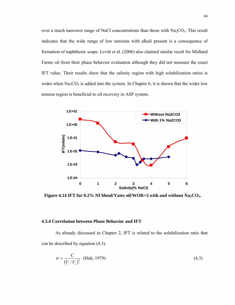
84

over a much narrower range of NaCl concentrations than those with Na2CO3. This result

indicates that the wide range of low tensions with alkali present is a consequence of

formation of naphthenic soaps. Levitt et al. (2006) also claimed similar result for Midland

Farms oil from their phase behavior evaluation although they did not measure the exact

IFT value. Their results show that the salinity region with high solubilization ratios is

wider when Na2CO3 is added into the system. In Chapter 6, it is shown that the wider low

tension region is beneficial to oil recovery in ASP system.

1.E-04

1.E-03

1.E-02

1.E-01

1.E+00

1.E+01

0 1 2 3 4 5Salinity(% NaCl)

IFT(

mN

/m

6

)

Without Na2CO3With 1% Na2CO3

Figure 4.14 IFT for 0.2% NI blend/Yates oil/WOR=3 with and without Na2CO3.

4.3.4 Correlation between Phase Behavior and IFT

As already discussed in Chapter 2, IFT is related to the solubilization ratio that

can be described by equation (4.3).

( )2/ si VVC

=σ (Huh, 1979) (4.3)

85

where σ : Interfacial tension (IFT)

Vi/Vs: Solubilization ratio

C: A constant with a typical value of 0.3.

The solubilization ratio (Vo/Vs) is the ratio of solubilized oil volume to surfactant

volume present (excluding soap) for the under-optimum samples. The volume of

solubilized oil can be measured by the difference between the volume of the initial oil in

the sample and that of the excess oil phase after equilibration. It represents a composite

value for the combined lower or middle phase microemulsion and colloidal dispersion

phase. As figure 4.15 shows for the salinity scan of 0.2% NI blend//1% Na2CO3/Yates

oil/WOR=3, solubilization ratio (Vo/Vs) increases from about 7 at 2% NaCl to about 20 at

3.4% NaCl, just below optimal salinity. For over-optimal samples, a similar calculation

can be made to obtain the value (Vw/Vs). Similar values were found for a scan with 0.5

wt% NI blend except that the salinities were higher with optimal salinity approximately

4.5% NaCl because the soap-to-surfactant ratio was smaller (Liu et al., 2006).

1

10

100

1000

2 2.5 3 3.5 4NaCl, %

Solu

biliz

atio

n ra

tio Vw/Vs

Vo/Vs

Figure 4.15 Solubilization ratios for 0.2% NI blend//1% Na2CO3/Yates

oil/WOR=3

86

In Huh’s correlation, (Vo/Vs) is used for calculating the IFT between

microemulsion and excess phase when the salinities are below the optimum condition and

(Vw/Vs) is used as the solubilization ratio when the salinities are above the optimum

condition. With the solubilization ratios and Huh’s correlation, the predicted IFT values

are shown in figure 4.16. The experimental IFT values are in good agreement with the

predicted values from solubilization ratios except at 3.6%-3.8% NaCl where the

measured value is higher. However, the measured value is ultra-low (around 10-3 mN/m)

and can mobilize oil.

1.E-04

1.E-03

1.E-02

1.E-01

2.0 2.5 3.0 3.5 4.0

NaCl, %

IFT,

mN

/m

.

Chun-huh Correlation

Spinning drop measurement

Figure 4.16 Comparison the IFT predicted from solubilization ratios and

measured IFT for 0.2% NI blend//1% Na2CO3/Yates oil/WOR=3

The solubilization ratios of 0.2% NI blend/1% Na2CO3/Midland Farm oil and

WOR=3 samples were also measured by phase behavior scan as shown in figure 4.17.

And the predicted IFT values and measured IFT values are shown in figure 4.18. Similar

to Yates oil, IFT from the solubilization ratios and the measured IFT are very close to

each other.

87

The results for Yates and Midland Farm oil indicate that IFT can be estimated by

measuring the solubilization ratios with phase behavior samples. For the PBB oil sample,

PBB Solubility Ratios after 40 days Settling (WOR=24, 0.2% NI)

1

10

100

1000

4 4.5 5 5.5 6x% NaCl (+ 1% Na2CO3)

Vw/V

s

1

10

100

1000

Vo/V

s

Vw/Vs Vo/Vs

Figure 4.17 Solubilization ratios for 0.2% NI blend//1% Na2CO3/Midland Farm

oil/WOR=3

1.E-04

1.E-03

1.E-02

1.E-01

1.0 1.5 2.0 2.5 3.0 3.5 4.0 4.5 5.0NaCl, %

IFT,

mN

/m

Chun-huh Correlation

Spinning drop measurement

Figure 4.18 Comparison the IFT predicted from solubilization ratios and measured IFT for 0.2% NI blend//1% Na2CO3/Midland Farm/WOR=3

88

the lower phases for under-optimum region are too dark to see through in the spinning

drop instrument. As a result, the oil drop diameter could not be measured because the

drop is obscured. Then, an alternative method to get the IFT value is with solubilization

ratios by observing the phase behavior samples. Also, it is much faster to obtain IFT by

using solubilization ratios than by spinning drop measurement. Figure 4.19 shows the

solubilization ratios of 0.2% NI blend/1% Na2CO3/PBB oil and WOR=24. Figure 4.20 is

the estimated IFT values from by the solubilization ratios in figure 4.19. The width of the

low tension region is from 4.0% NaCl to 5.5% NaCl. Because of the difficulties in

accurately measuring the phase volume with such a high WOR (24), salinities lower than

4.0% NaCl or higher than 6.0% NaCl were not included in figure 4.19. The lowest IFT

value at optimum condition is still around 10-3 mN/m. This result suggests that NI blend

is also a good IFT reduction agent for PBB oil.

1

10

100

1000

4 4.5 5 5.5x% NaCl (+ 1% Na2CO3)

Solu

biliz

atio

n ra

tio

V w/V s

V o/V s

6

Figure 4.19 Solubilization ratios for 0.2% NI blend//1% Na2CO3/PBB

oil/WOR=24

89

1.00E-04

1.00E-03

1.00E-02

1.00E-01

1.00E+00

4 4.5 5 5.5 6x% NaCl (+ 1% Na2CO3)

IFT

(mN

m)

Figure 4.20 IFT predicted from solubilization ratios for 0.2% NI blend//1%

Na2CO3/PBB oil/WOR=24

4.3.5 Dynamic IFT and equilibrium IFT

All the previous IFT measurements are equilibrium IFT measurements, i.e., the

surfactant solution and crude oil has been mixed and reached equilibrium before the

spinning drop measurement. However, many researchers have used dynamic IFT

measurement, in which a fresh crude oil drop is directly injected into spinning tube with

the alkali surfactant solution. If dynamic IFT is for surfactant system without alkali, it

might be possibly correct because the optimum condition is not a function of water oil

ratio for pure surfactant system. However, it is not suitable for alkali surfactant system

because optimum salinity is a function of water oil ratio, as discussed in the previous

chapter. If dynamic method is used, it is applicable only for very high water oil ratio

because the system consists of only a single oil drop and a whole tube of alkali surfactant

90

solution. Furthermore, the natural soap is generated at the oil water interface due to the

reaction of alkali and naphthenic acid in the oil drop, and the soap and surfactant will

transfer to aqueous phase or stay in oleic phase depending on the phase behavior. In

many cases, this effect will cause a transient ultra-low tension because soap and

surfactant will be at the interface for some time and then desorbed. Figure 4.21 shows an

example for dynamic IFT. A fresh oil drop was injected into a spinning tube full of 0.2%

NI Blend, 1% Na2CO3 and 1% NaCl solution at ambient temperature. In this case, it is

under-optimum phase behavior because water oil ratio is very high so that the soap to

surfactant ratio is very low. The soap is generated at oil water interface and transfers to

the aqueous phase. At 20 minutes, most soap was at interface so that an ultra-low tension

was observed. When soap left the interface and went to the aqueous phase, the IFT

bounced up by approximately two orders of magnitude. IFT will be low at equilibrium

only when the aqueous solution is near optimum conditions for the surfactant.

Dynamic IFT of fresh oil and 0.2%NI-1%Na2CO3-1%NaCl

1.E-04

1.E-03

1.E-02

1.E-01

1.E+00

0 50 100 150 200 250 300Time, minutes

IFT,

mN

/m

Figure 4.21 Dynamic IFT of fresh Yates oil and 0.2% NI Blend / 1% Na2CO3 /

1% NaCl

91

In some papers, existence of a transient ultra-low IFT was reported to be an

adequate criterion for a good surfactant formulation. As figure 4.21 shows, it is not

correct because the real equilibrium IFT might be much higher. In the reservoir, it is not a

transient minimal IFT but the equilibrium IFT that generates high capillary number

because of the time scale of flooding process. It takes years to finish a flooding process.

Therefore, equilibrium IFT as discussed in the previous sections should be used for

designing alkali surfactant processes.

92

Chapter 5

Chemical Consumptions of Alkali Surfactant Process

An ASP process is feasible only when the cost of chemical consumptions is small.

It is very crucial to limit the chemical consumptions, such as surfactant adsorption, alkali

precipitation. This chapter shows how to measure and control the chemical consumptions.

As discussed in Chapter 2, surfactant adsorption is very important for the

surfactant consumption. In this section, both static and dynamic experiments are

performed to evaluate the adsorption of surfactant on dolomite. The static test is the

bottle test for surfactant adsorption on porous media by shaking and settling. The

dynamic experiments are the flow experiments where the breakthrough of the surfactants

is compared with that of a non-adsorbing tracer, which is chloride ion determined by

conductivity measurement in this research.

5.1 Static Adsorption of Surfactant

5.1.1 Static Adsorption Experimental Procedure

The static adsorption experiments were performed in the following procedure.

The initial surfactant solution has a fixed concentration that can be accurately determined

by Potentiometric titration (See Appendix A) with Benzethonium Chloride (hyamine

93

1622). Then the surfactant solution was mixed with the porous medium, such as calcite

powder or dolomite powder, at varied weight ratios in centrifuge tubes. If the powder

amount is large so that the powder agglomerates, the Branson® Sonifier 450 can be used

to sonicate the powder and solution mixture for at least 1 minute. After the powder was

well dispersed in the solution, the samples were put on a rotating shaker and shaken for at

least 24 hours. Afterwards, the samples were centrifuged at 3000 rpm for at least 30

minutes. Finally, the equilibrium surfactant concentrations of the liquid phase were

determined again by potentiometric titration. By comparing the initial and equilibrium

surfactant concentration, the amount of surfactant adsorbed on the surface can be

obtained. Because the porous media surface area can be determined by BET adsorption,

surfactant adsorption density was calculated. Three carbonate porous medium samples

with different surface areas were tested. The three samples are calcite powder

(SOCAL31® from Solvay Performance Chemicals, BET area: 17.9 m2/gram), dolomite

powder (Carpool® from Earth Safe Organics, BET area: 1.7 m2/gram) and dolomite sand

(from Unimin corporation, BET area: 0.3 m2/gram).

5.1.2 Static Adsorption Results for Anionic surfactant

Two surfactant formulations, NI blend and TC blend, which have been introduced

in Chapter 3, are used to test anionic surfactant adsorption on carbonate.

5.1.2.1 TC Blend

The adsorption of TC blend on dolomite with or without sodium carbonate is

shown in Figure 5.1. The initial surfactant concentration was fixed at either 0.05% or

0.1% (active material). The specific surface area of dolomite powder determined by the

94

BET adsorption is 1.7m2/gram dolomite powder. The adsorption isotherm in the absence

of sodium carbonate is similar to a Langmuir adsorption isotherm with a plateau

adsorption of about 0.002 mmol/m2 or 1.2 mg (surfactant)/gram (dolomite). Addition of

0.2-0.4 M sodium carbonate reduced the adsorption by a factor of 10 and the saturation

plateau is about 2×10-4 mmol/m2 or around 0.1 mg (surfactant)/gram (dolomite). This

result is consistent with previous results in the adsorption of TC blend on calcite powder,

which show sodium carbonate can significantly reduce the adsorption (Hirasaki and

Zhang, 2002). The reduction of adsorption may be attributed to change surface charge to

negative charge by the addition of carbonate ion, which is a constituent ion of carbonate

formation and is a potential determining ion.

0.0

0.2

0.4

0.6

0.8

1.0

1.2

0.00 0.02 0.04 0.06 0.08 0.10 0.12Surfactant Concentration (Wt%)

Ads

orpt

ion

Den

sity

(m

g/m

2 )

WithNa2CO3(0.2M,0.3M,0.4M)

Figure 5.1 Adsorption on powdered dolomite of TC blend with/without Na2CO3

95

5.1.2.2 Test of Other Potential Determining Ions

Other potential determining ions were tested for the adsorption of TC blend on the

same dolomite powder (BET 1.7m2/gram). Hydroxyl ion can change the zeta potential of

the carbonate/brine interface from positive charge to negative charge by raising the pH

(Thompson and Pownall, 1989).

0.0

0.2

0.4

0.6

0.8

1.0

1.2

0.00 0.02 0.04 0.06 0.08 0.10 0.12Residual Surfactant Concentration (Wt%)

Ads

orpt

ion

Den

sity

(m

g/m

2 )

Surfactant only

With 0.1 M NaOH

With 0.1M NaOH+0.15M Na2SO4

Figure 5.2 Adsorption of TC blend on dolomite with hydroxyl ion and sulfate ion

Hydroxyl ion can change the pH so that the zeta potential of the carbonate/brine

interface changes from positive charge to negative charge (Thompson and Pownall, 1989).

In a fractured chalk formation, Austad and Strand et al. (2005) used sulfate ion to alter

the surface potential of chalk surface. However, either hydroxyl ion or sulfate ion could

not decrease the surfactant adsorption on dolomite surface. As figures 5.2 shows, the

adsorption amount on dolomite surface with these ions is the same as those without any

96

potential determining ion. It seems that between carbonate, hydroxyl and sulfate ions,

only carbonate ion can reduce the adsorption on the dolomite surface.

5.1.2.3 Surfactant Adsorption on Different Surface Area

Surface area of the porous media has remarkable effect on the surfactant

adsorption. As mentioned in the previous part, three carbonate porous medium samples

with different surface areas were tested. They are calcite powder (17.9 m2/gram),

dolomite powder (1.7 m2/gram) and dolomite sand (0.3 m2/gram). Figure 5.3 shows that

the adsorptions of TC blend on the three samples are close to each other if the adsorption

is calculated by using surfactant adsorption amount per porous media surface area.

However, if the adsorption is calculated by using surfactant adsorption amount per

porous media weight as in figure 5.4, the adsorptions on the three samples are very

different, even though the mineralogy of the three samples is similar. These results imply

that it is the surface area, not the weight, of the porous media that should be used to

compare the adsorption. For static adsorption experiments, samples with larger surface

areas will adsorb more surfactant, so that it is more accurate for adsorption measurement

because the difference between the residual surfactant concentration after the surfactant

and solid mixing and initial surfactant concentration is significant. Thus, the calcite

powder was used in the static adsorption experiments hereafter.

97

0.0

0.2

0.4

0.6

0.8

1.0

1.2

0.00 0.02 0.04 0.06 0.08 0.10 0.12

Surfactant Concentration (Wt%)

Ads

orpt

ion

Den

sity

(mg/

m 2 )

Adsorption of dolomite powder (1.7m2/g)

Adsorption of dolomite sand (0.3m2/g)

Adsorption of calcite powder (17.9m2/g)

Figure 5.3 Adsorption of TC blend on different samples per surface area

0

2

4

6

8

10

12

14

16

18

20

0.00 0.02 0.04 0.06 0.08 0.10 0.12

Surfactant Concentration (Wt%)

Ads

orpt

ion

dens

ity (m

g/g)

Adsorption of dolomite powder (1.7m2/g) without alkali

Adsorption of dolomite sand (0.3m2/g) without alkali

Adsorption of calcite powder (17.9m2/g)

Figure 5.4 Adsorption of TC blend on different samples by using weight of porous media

98

5.1.2.4 NI Blend

As introduced in Chapter 3, NI blend is a mixture of N67 and IOS. The adsorption

isotherms of N67 and IOS on calcite powder for solutions containing no NaCl and either

0% or 1% Na2CO3 are shown in figure 5.5 and 5.6. Similar to TC blend, the adsorptions

of both N67 and IOS were greatly reduced around an order of magnitude by addition of

Na2CO3 because carbonate ions reverse the charge of the calcite surface from positive to

negative so that anionic surfactant ions are repulsed (Zhang et al, 2005).

0.0

0.5

1.0

1.5

2.0

2.5

3.0

3.5

0.00 0.02 0.04 0.06 0.08 0.10 0.12 0.14Surfactant Concentration (%)

Ads

orpt

ion

Den

sity

, mg/

m 2

0% NaCl, 0% Na2CO3 0% NaCl, 1% Na2CO3

Figure 5.5 Adsorption of N67 on calcite powder (17.9 m2/g) with or without 1 % Na2CO3 and with no NaCl.

99

0.0

0.5

1.0

1.5

2.0

2.5

3.0

3.5

0.00 0.02 0.04 0.06 0.08 0.10 0.12 0.14Surfactant Concentration (%)

Ads

orpt

ion

Den

sity

, mg/

m 2

0% NaCl, 0% Na2CO3 0% NaCl, 1% Na2CO3

Figure 5.6 Adsorption of IOS on calcite powder (17.9 m2/g) with or without 1 % Na2CO3 and with no NaCl.

Adsorption is approximately 2.8 and 3.0 mg/m2 in the plateau regions for the

respective surfactants in the absence of Na2CO3, corresponding to 0.47 and 0.23

nm2/molecule, assuming a uniform monolayer. The latter number (for IOS) is close to

the area of a single straight hydrocarbon chain. Since this surfactant consists of a mixture

of molecules with the sulfonate group located at various places along the hydrocarbon

chain, the adsorbed molecules are twin-tailed. As a result, their area per molecule should

be about twice that of a single chain, and it seems likely that an adsorbed bilayer exists in

the plateau region. Bilayers often form for adsorption of surfactant ions on surfaces of

opposite charge at concentrations near and above the critical micelle concentration

(CMC). This is because bilayers expose a polar surface, which has a low free energy with

the aqueous phase. The arrangement of adsorbed molecules for N67 is not clear.

100

Figure 5.7 shows adsorption isotherms of the NI blend on calcite powder at

different NaCl concentrations with and without 1 wt% Na2CO3. In the absence of NaCl

adsorption is comparable to that of N67 or IOS alone. As NaCl concentration increases,

the beneficial effect of Na2CO3 is reduced, presumably because the screening effect of the

additional electrolyte decreases electrostatic repulsion between surfactant ions in solution

and the calcite surface. Nevertheless, Na2CO3 reduces adsorption by more than a factor

of three for 3 wt% NaCl.

0.0

0.5

1.0

1.5

2.0

2.5

3.0

3.5

0.00 0.05 0.10 0.15Surfactant Concentration (Wt%)

Ads

orpt

ion

Den

sity

, m

g/m

2

5% NaCl, 0% Na2CO3 5% NaCl with 1.21% Na2CO33% NaCl, 0% Na2CO3 3% NaCl, 1.21% Na2CO30% NaCl, 0% Na2CO3 0% NaCl, with 1.0%Na2CO3

Figure 5.7 Adsorption of NI blend on calcite as a function of NaCl content with and without 1 wt% Na2CO3.

In the previous static adsorption experiments, approximately 1% Na2CO3 was

used as adsorption reduction agent. It is also important to know how much Na2CO3 is

needed to have this adsorption reduction effect. The threshold of Na2CO3 concentration at

which the adsorption reduction effect occurs is shown as figure 5.8. The initial surfactant

101

concentration is fixed at 0.06% without any NaCl, but the Na2CO3 concentration is

varied. The ratio of calcite powder and surfactant solution was also fixed and the two

were mixed. Then the residual surfactant concentration after mixing was measured. It is

found that the adsorption changes with the Na2CO3 concentration as shown by figure 5.8.

The adsorption reduction effect seemed the same when the Na2CO3 concentration was

higher than 0.1 %, i.e., further increasing the Na2CO3 concentration does not further

decrease the surfactant adsorption. However, the adsorption will increase as the Na2CO3

concentration deceases when it is lower than 0.1%. From this result, the lowest alkali

concentration for lowering the surfactant adsorption on calcite should be higher than

0.1% Na2CO3. Figure 5.9 indicates that with 5% NaCl, increasing the Na2CO3

concentration more than 0.18% will not further decrease the surfactant adsorption.

However, the threshold concentration could be lower since data were not obtained

between 0 and 0.18% Na2CO3.

0.00

0.05

0.10

0.15

0.20

0.25

0.30

0 0.1 0.2 0.3 0.4 0.5 0.6%Na2CO3

Ads

orpt

ion

Den

sity

, m

g/m

2

Figure 5.8 Test of threshold concentration of Na2CO3 for the adsorption.

102

0.0

0.5

1.0

1.5

2.0

2.5

3.0

3.5

0.00 0.05 0.10 0.15Surfactant Concentration (%Wt)

Ads

orpt

ion

Den

sity

, mg/

m 2

5% NaCl, 0% Na2CO3 5% NaCl with 0.178% Na2CO35% NaCl with 0.404% Na2CO3 5% NaCl with 1.21% Na2CO3

Figure 5.9 Adsorption of NI blend on calcite at 5% NaCl with different Na2CO3.

By summarizing those data in figures 5.7 to 5.9 and additional experiments with

different NaCl and Na2CO3 concentrations, the contours of plateau adsorption for NI

blend are plotted as Figure 5.10. This plot shows that the domain with surfactant

adsorption less than 1 mg/m2 is: [Na2CO3]>0.2% and [NaCl] <3%. Hence, it’s better to

perform the alkali-surfactant process with this anionic surfactant (NI blend) in this

concentration range for low surfactant adsorption.

103

Figure 5.10 Contour of Plateau Adsorption (mg/m2) for NI Blend on calcite.

5.1.2.5 Adsorption of Nonionic Surfactant and Anionic Surfactant

Nonionic surfactant is not generally considered as a candidate for surfactant EOR

process because its adsorption on sandstone formation is very large comparing to anionic

surfactant. A nonionic surfactant, Nonylphenol-12EO-3PO (from Harcros Chem), was

tested in the same static procedure as the anionic surfactant except the UV-vis spectrum

was used to determine the nonionic surfactant concentration. The UV (ultra-violet)

absorbent peak of this surfactant is at 277nm. There is a linear relationship between the

absorbency at 277 nm and surfactant concentration when the concentration is less than

0.2 wt% so that the surfactant concentration can be accurately measured.

104

0.0

0.1

0.2

0.3

0.4

0.5

0.6

0.7

0.8

0.9

0.00 0.02 0.04 0.06 0.08 0.10 0.12

Surfactant Concentration(Wt%)

Ads

orpt

ion

Den

sity

(mg/

m 2 ) Nonylphenol-12EO-3PO on silica

Plateau184 Å2/molecule.

CS330 on silica5000 Å2/molecule

Figure 5.11 Comparison the adsorption on silica sand between nonionic

surfactant and anionic surfactant

Figure 5.11 shows that this nonionic surfactant has much higher adsorption on

silica sand (from US Silica®, BET area: 3.6mg/gram) than the anionic surfactant (CS330)

as expected. The high nonionic surfactant adsorption on silica surface is because the

hydrogen bond between the nonionic surfactant and silica surface will help the nonionic

surfactant attach the surface of silica because silica surface also has hydroxyl group.

However, on dolomite surface, hydrogen bond between the carbonate surface and

nonionic surfactant is not expected. Thus carbonate surface will not attract the nonionic

surfactant. As figure 5.12 illustrates, the adsorption of nonionic surfactant is much lower

than that of anionic surfactant in the absence of Na2CO3 and is in the same magnitude of

105

that of anionic surfactant with presence of Na2CO3. This result indicates that the nonionic

surfactant is also a candidate for carbonate formations from the adsorption point of view.

0.0

0.2

0.4

0.6

0.8

1.0

1.2

0.00 0.02 0.04 0.06 0.08 0.10 0.12 0.14

Residual Surfactant Concentration(Wt%)

Ads

orpt

ion

Den

sity

(mg/

m2 )

Anionic surfactant on dolomite without alkali, plateau=83 Å2/molecule

Nonionic surfactant on dolomite plateau=714 Å2/molecule

Anionic surfactantwith Na2CO3(0.2M,0.3M,0.4M)plateau = 830 Å2/molecule

Figure 5.12 Comparison the adsorption on dolomite powder between nonionic

surfactant and anionic surfactant.

5.2 Dynamic Adsorption of Surfactant

Dynamic adsorption experiment measures the surfactant adsorption by surfactant

flooding in one dimensional sand pack or core. By comparing the breakthrough history of

surfactant and non-adsorbing tracer, the adsorption can be determined. Although the

dynamic method is much more complicated and takes much longer time than the static

adsorption method, it is still widely used to estimate the surfactant consumption because

it is analogous to the actual surfactant flooding process (Griggs and Bai, 2005).

106

Furthermore, the dynamic method can provide the information about the kinetic effects of

adsorption.

5.2.1 Dynamic Adsorption Experimental Procedure

Dynamic adsorption experiments on the silica sand, dolomite sand and dolomite

cores were performed in a one-foot column packed with sand. The experimental

apparatus diagram is shown in figure 5.13.

Syringe Pump

1-d column

Computer

(Monitoring pressure)

Surfactant solution

with NaCl

Sample Collection

Figure 5.13 Schematic Experimental Apparatus

The experimental procedure is:

1. Fill the column with formation brine.

2. Inject the surfactant solution into the column by the pump; the solution also

contains sodium chloride as a non-absorbing tracer.

3. Collect the effluent at different times and measure the concentration of the

surfactant and sodium chloride to obtain the breakthrough curves of the two components

107

4. For the silica sand pack, isobutyl alcohol and de-ionized water are used to wash

the column for the next experiment. For dolomite sand pack or dolomite cores, the

column is repacked with fresh dolomite sand for the next experiment because the

adsorbed surfactant could not be totally removed by the washing process.

In the experiment, the conductivity of the solution was used to measure the NaCl

concentration, and potentiometric titration was used to measure the surfactant

concentration as in the static experiments. Because the ionic surfactant may affect the

conductivity of the water, an auxiliary experiment was performed to determine whether

this effect would introduce error in measuring the NaCl for the surfactant and NaCl

concentration used here. The results showed that there was not a significant error induced

by the ionic surfactants. Furthermore, equations (5.1) for NaCl concentration less than 0.5

wt%, which were obtained from the experiments, can be used to calculate the NaCl

concentration. In the dynamic experiments, the NaCl concentration can be obtained by

measuring the diluted effluent.

[Conductivity]= 16905*[NaCl Wt%]+ 30±140. or [NaCl Wt%]= 5.92*10-5*[Conductivity]- 2*10-3±8*10-3 (5.1)

5.2.2 Dynamic Adsorption Model

In order to obtain the adsorption by analyzing the breakthrough history, a

dynamic adsorption model is introduced in this section. Below is a brief description of

the one dimensional adsorption model. The major assumptions of the model are:

1. No velocity in the r and θ directions, i.e., one-dimensional flow

108

2. The adsorption isotherm can be approximated with a constant slope over the

range of concentration studied, i.e., the adsorption is linear with the local concentration.

The actual adsorption is a Langmuir type isotherm as shown in those static adsorption

isotherms, e.g. figure 5.7. This assumption is made so that an analytical solution can be

obtained.

3. The physical properties, such as viscosities and densities etc., do not change

with any component concentration of the solute.

4. The dispersion coefficient Kl is assumed to be proportional to velocity and the

velocity is constant, i.e. the dispersion is constant.

5. The medium is homogeneous.

With these assumptions, the mass conservation equation with adsorption is as

follows:

2

2

)1(xcK

xcu

tc

l ∂∂

=∂∂

+∂∂

+ φβφ x>0, t>0 (5.2)

where φ is the porosity.

Kl is the dispersion coefficient.

The cord slope of the adsorption isotherm with respect to the reduced

concentration is denoted by β. β can be calculated from the static adsorption isotherm by

using the equation (5.3). Because the actual surfactant adsorption isotherm is not a linear

isotherm, the chord on the isotherm between zero and local concentration was used as the

β.

isos Sk

cc

ρφφβ )1( −

== (5.3)

where φ is the porosity of the porous medium

109

ρdolomite is the density of the porous medium

S is the BET surface area of the porous medium

kiso is the cord slope of the isotherm plot from static adsorption isotherms

The concentration is transformed to a reduced concentration that has a range

between 0 and 1. Hereafter, the concentration used here is the dimensionless

concentration. Thus the boundary conditions and the initial conditions are:

c (x, 0) =cIC=0, x>0

c (0, t) =cBC=1, t>0

0),( =∞∂∂ txc , t>0

By using interstitial velocity v=u/φ, the differential equation can be translated to:

2

2

)1()1( xcK

xcv

tc l

∂∂

+=

∂∂

++

∂∂

ββ (5.4) In the absence of dispersion, the analytical solution to this differential equation is

an indifferent step wave with a velocity equal to )1/( β+v . Thus the cord slope of the

adsorption isotherm describes the retardation of the concentration wave. By transforming

the variables, this partial difference equation (PDE) can be reduced into an ordinary

difference equation (ODE).

0ddC2

dCd2

2

=η

η+η where β

βη

+

+−

=

141

tK

vtx

l

(5.5)

By integrating the ODE, the solution obtained is:

)(erfc2121

21

0

2

ηηπ

ηη =

⎥⎥⎦

⎤

⎢⎢⎣

⎡−= ∫ − deC

(5.6)

110

With the characteristic system length L, the distance variable will be made

dimensionless with respect to L. Thus the non-dimensional variable η is:

)1(Pet2

)1(tx

D

DD

β+

β+−

=η

(5.7)

where ,LxxD /= ALuAttD φ/= and lKLvPe /= .

The effluent history, i.e., the concentration history at xD=1 can be obtained. And

the retardation of the break-through curve can be expressed as β. If the nonabsorbent

tracer and adsorbing solute break-through curves coincide, then β=0, that is no adsorption

occurred for the component measured.

Since the data obtained are the effluent history, the value of β and Peclet number

(Pe) can be calculated by following manipulation. From the relation of the

complementary error function to the cumulative Gaussian probability distribution, the

slope of adsorption isotherm and the Peclet number can be estimated by the mean and

standard deviation of a Gaussian distribution. The cumulative Gaussian probability

distribution is given by the following formula:

⎥⎦

⎤⎢⎣

⎡⎟⎟⎠

⎞⎜⎜⎝

⎛+=

21

21}{ uerfyP (5.8)

σμ−

=yu (5.9)

uy σμ += (5.10)

where μ and σ are the mean and standard deviation of the Gaussian distribution.

Recall that the effluent concentration is given by equation (5.6) as.

111

] where

)1(2

)1(1

β

βη

+

+−

=

Pet

t

D

D

(5.11) [ )(121)(

21 ηη erferfcC −==

Next the variables are transformed such that the transformed variables are a

cumulative Gaussian distribution. First, transform C such that it has the same dependence

on the error function as the Gaussian distribution.

[ ] PCerf ⇒−=+ 1)(121 η

(5.12)

The argument of the error function should map the independent variables:

2)1(2

1

)1(2

)1(1

)1( u

Pet

t

Pet

t

xD

D

D

D

D ⇒+

−+=

+

+−

==β

β

β

βη and ytt

D

D ⇒−1

Finally, the expressions for μ and σ are: βμ −= and Peβσ +

≈12

.

From the experimental data c and the tD, Pe, y and η can be calculated. With y and

η, μ and σ can be calculated by linear regression. Then β and Pe are obtained.

Since the exact porosities of the sand packs or cores are unknown, they should be

determined first. The fact that there is no adsorption for NaCl in the sand or the dolomite

can be used to estimate the porosity. For the NaCl data, a pore volume is guessed at first,

and then the μ and σ are calculated based on the guessed pore volume. Because β equals

zero for no adsorption case, the porosity for which β=0 would be the actual porosity. The

porosity (0.34) calculated by this method is close to the porosity that comes from the

weight method (0.35). With the calculated porosity, we can obtain the β and Peclet

112

Number by using the linear regression for the surfactant data. The simulation curve also

can be plotted with the calculated β and Peclet Number.

5.2.3 Dynamic Adsorption of Anionic Surfactant

Figure 5.14 shows the break-through curve and simulation curve of TC blend in

silica sand.

0.00.10.20.30.40.50.60.70.80.91.0

0.0 0.5 1.0 1.5 2.0 2.5 3.0

Injected Volume (PV)

Dim

ensi

onle

ss C

once

ntra

tion

Experimental Data for NaCl

Experimental Data forCS330+TDA-4POSimulation Curve forCS330+TDA-4POSimulation Curve for NaCl

0.1% CS330+0.1%TDA-4PObeta=0.04±0.04PV=49±1mlPorosity=0.329±0.008

Figure 5.14 Dynamic Adsorption of TC Blend in silica sand column

From this plot, no significant adsorption for TC blend is found in the silica sand

(From US Silica® BET: 0.25 mg/g) packed column because the break-through curves of

the two components (NaCl and surfactant) superimpose each other. Also this one-

dimensional model can simulate this displacement experiment very well. The value of β

is only 0.04, which also indicates that the adsorption amount is very small. The two

components of TC blend, TDA-4PO and CS330, were also tested by the dynamic method

113

respectively. Both β values of these two surfactants are 0.02, which is also quite small.

The reason that the adsorption of anionic surfactant is negligible on the silica surface is

due to the negatively charged interface of brine/silica, which repels the negatively

charged surfactant by electrostatic forces.

0.00.10.20.30.40.50.60.70.80.91.0

0.0 0.5 1.0 1.5 2.0 2.5 3.0


Dim

ensi

onle

ss C

once

ntra

tion


Experimental Data for CS330

Simulation Curve for CS330

Simulation Curve for NaCl

0.1%CS330beta=0.27±0.04PV=21.6±0.4mlPorosity=0.171±0.003

Figure 5.15 Dynamic Adsorption of CS 330 in dolomite core

On dolomite surface, the dynamic adsorption of the anionic surfactant is much

greater. Figure 5.15 shows the break-through curve and the simulation curve of CS330

and NaCl in the dolomite core from Yates (permeability is 122~284 md; porosity is

0.171±0.003). The break-through curve for CS330 has some lag compared with the

break-through of NaCl. This means the dolomite core adsorbs a certain amount of

surfactant so that it breaks through later. From the simulation result, β is estimated as

β=0.27±0.04, which is much larger than that in the silica sand pack. Because the core

samples are not identical and the BET surface area of the core could not be measured,

114

crushed dolomite sand will be used as an alternative carbonate media for the remaining

dynamic adsorption experiments.

As mentioned in previous section, the surface area of crushed dolomite sand that

was determined by the BET adsorption is 0.3 m2/gram sand. With the porosity and

dolomite density, β can be calculated by using equation (5.3), assuming the adsorption

density, i.e., the adsorption amount per active surface area is not changed. Then, the

adsorption from the static method and dynamic method can be compared as shown in

figure 5.16. The break-through curve and the simulation curve of the surfactant mixture

and NaCl for dolomite sand pack column (porosity is 0.34) are plotted in Figure 5.16.

0.0

0.1

0.2

0.3

0.4

0.5

0.6

0.7

0.8

0.9

1.0

0.0 0.5 1.0 1.5 2.0 2.5 3.0Injected Volume (PV)

Dim

ensi

onle

ss C

once

ntra

tion

Expr. 2 Data for NaClExpr.2 Data for SurfactantSimulation for Expr.2 SurfactantSimulation for Expr.2 NaClExpr.1 Data for NaClExpr.1 Data for SurfactantSimulation for Expr. 1 SurfactantSimulation for Expr.1 NaClcalculated from isotherm

Expr. 2v=12 feet/daybeta=0.22±0.03

0.1%CS330+0.1%TDA-4POExpr. 1v=1.2 feet/daybeta=0.34±0.03 Cl-

Expr. 2

Calculated from dolomite isothermbeta=0.40

Expr. 1

Figure 5.16 Adsorption of TC blend in dolomite sand column without Na2CO3

Figure 5.16 points out that the adsorption of surfactant on dolomite sand is

significant. It also demonstrates that the adsorption of surfactants is not an instantaneous

process and depends on the flow rate. At a high interstitial velocity of 12 feet/day

115

(β=0.22), the retardation is much smaller than that at 1.2 feet/day (β=0.34). Even at the

lower flow rate, β is less than that calculated from the static adsorption isotherm

(β=0.40).

0.0

0.1

0.2

0.3

0.4

0.5

0.6

0.7

0.8

0.9

1.0

0.0 0.5 1.0 1.5 2.0 2.5 3.


Dim

ensi

onle

ss C

once

ntra

tion

0


Experimental Data for Surfactant

Simulation Curve for Surfactant

Simulation Curve for NaCl

0.1%CS330+0.1%TDA-4PO +0.3MNa2CO3

beta=0.07±0.04v=1.2 feet/day

Figure 5.17 Adsorption of TC blend in dolomite sand column with Na2CO3

Similar to what was found in static adsorption, the addition of sodium carbonate

can significantly reduce surfactant adsorption, as shown in Figure 5.17. At the same slow

flow rate, β is reduced from 0.34 to 0.07 by adding 0.3 M Na2CO3.

Table 5.1 summarizes the dynamic adsorption results.

116

Porous Media From Permeability Porosity Pore

volume Inject

Surfactant Flow rate

Retardation β

Silica sand (BET:

0.2m2/g)

US Silica Ottawa

Foundry ~120 darcy

0.329 ±0.008

49±1ml

CS330 (0.1%)

8 feet/day 0.02 ±0.03

Silica sand (BET:

0.2m2/g)

US Silica Ottawa

Foundry ~120 darcy

0.329 ±0.008

49±1ml TDA-4PO

(0.1%) 8

feet/day 0.02 ±0.03

Silica sand (BET:

0.2m2/g)

US Silica Ottawa

Foundry ~120 darcy

0.329 ±0.008

49±1ml TC Blend

(0.2%) 8

feet/day 0.04 ±0.04

Dolomite core

Marathon Oil

Company

122~284 md

0.171 ±0.003

21.6±0.4 ml

CS330 (0.1%)

5 feet/day 0.27 ±0.03

Dolomite sand BET:

0.3m2/g

Unimin corporation ~40 darcy

0.335 ±0.008

50±1ml

TC Blend (0.2%)

1.2 feet/day 0.34 ±0.03

Dolomite sand (BET:

0.3m2/g


0.338 ±0.008

50±1ml

TC Blend (0.2%)

12 feet/day 0.22 ±0.03

Dolomite sand (BET:

0.2m2/g)


0.337 ±0.008

50±1ml

TC Blend (0.2%) Na2CO3 (0.3M)

1.2 feet/day 0.07 ±0.04

Table 5.1 Summarization of dynamic adsorption experiments’ condition and

results.

5.3 Sodium carbonate consumption by gypsum

Pure calcite does not consume much alkali. However, the consumption of alkali in

carbonate reservoir may be a crucial problem because of the precipitation reaction of

alkali with gypsum or anhydrite. Because the solubility products of CaCO3 and CaSO4

are 4.96*10-9 and 7.10*10–5 respectively (CRC Handbook, 68th Edition), it is a serious

problem to apply Na2CO3 as the alkali candidate in the presence of gypsum or anhydrite

because of the precipitation reaction shown as equation (5.13).

−− +↓→+ 2434

23 SOCaCOCaSOCO (5.13)

117

By using the same analysis as in dynamic surfactant adsorption, figure 5.18 shows

the retardation for a porous medium with porosity 0.3. It illustrates that the retardation is

significant. For a 0.1M (~1%) Na2CO3, the concentration usually being considered for oil

recovery processes, the retardation is around 0.7 PV for the condition that 0.1% of the

porous medium is CaSO4. Although the propagation velocity of sodium carbonate can be

increased by raising the injection alkali concentration, the total amount of alkali

consumption will not change. It is impractical to solve this problem by increasing the

sulfate ion concentration through adding Na2SO4 because of the tremendous difference

between the two solubility products. Although this calculation is approximate because

they are based on room temperature value of solubility products and neglect activity

coefficients, the point made here is that other alkali should be considered when gypsum is

present.

1.E-03

1.E-02

1.E-01

1.E+00

1.E+01

1.E+02

1.E+03

1.E+04

0 0.2 0.4 0.6 0.8 1Na2CO3 injection concentration (mol/L)

Ret

arda

tion

Tim

e (P

V)

All the medium is CaSO410% of the medium is CaSO41% of the medium is CaSO4

0.1% of the medium is CaSO40.01% of the medium is CaSO4

Figure 5.18 Relationships between retardation and CaSO4 fraction in porous

medium (porosity=0.3)

118

NaHCO3 with Na2SO4 may be a potential choice for the situation with CaSO4.

NaHCO3 has much lower carbonate ion concentration and additional sulfate ions can

decrease calcium ion concentration in the solution. However, this method is not

applicable again. The concentration of CO32- is around the one hundredth the

concentration of NaHCO3 for a NaHCO3 solution so that large amount Na2SO4 is needed

to avoid precipitation of CaCO3. For a 0.1M NaHCO3 solution, the carbonate ion

concentration is around 1.0*10-3 M, and we need 14 M Na2SO4 to prevent the

precipitation of CaCO3.

The other alkali candidate is NaOH with Na2SO4 since the solubility product of

Ca(OH)2 is 4.68*10-6. The reaction between NaOH with Na2SO4 is shown as equation

(5.14). The minimum Na2SO4 concentration that restrains the Ca(OH)2 precipitation can

be calculated by equation (5.15). For a 0.1 M NaOH solution, 0.15 M Na2SO4 is needed

to suppress the calcium ion concentration so that no Ca(OH)2 will precipitate. Higher

Na2SO4 is necessary with higher NaOH concentration. However, the adsorption of

anionic surfactant will not decreased by NaOH formulation.

4224 )(2 SONaOHCaCaSONaOH +⇔+ (5.14)

2

)(

224 ][*15][][

2

4 −−− == OHKK

OHSOOHspCa

spCaSO (5.15)

Some organic alkalis, such as sodium citrate, sodium metaborate, might be the

alternate choices when gypsum is present because calcium citrate or calcium metaborate

has larger solubility product than calcium sulfate. Further studies should be done in this

area.

119

Chapter 6

Simulation and Optimization of Alkaline Surfactant Polymer

Process

A one-dimensional simulator was developed and used in this chapter to show

characteristics of ASP process with the IFT properties of alkali–surfactant system shown

in previous chapters.

6.1 One-dimensional Simulator

The synergic effect of synthetic surfactant and soap are very important for the

success of ASP process as shown in the phase behavior and interfacial tension results in

Chapters 3 and 4. However, because current reservoir simulators do not include soap

component, they do not have the capacity to evaluate the characteristics of the ASP

process. In order to understand the ASP process, a one-dimensional, two phase, multi-

componential simulator was developed to calculate the profiles and oil recovery as a

function of process variables. In this simulator, the main relationships are as follows:

(1) Phase behavior and interfacial tension are functions of alkali，electrolyte (NaCl),

surfactant and natural soap concentrations,

(2) Fractional flow curves are functions of interfacial tension, phase saturation and

viscosity of each phase,

120

(3) Surfactant adsorption is a function of surfactant concentration in aqueous phase, alkali

concentration and salinity,

(4) Natural soap is generated from the naphthenic acids contacted by the alkali,

(5) Physical dispersion is described by convective dispersion, i.e, proportional to velocity

(6) Aqueous phase viscosity is a function of electrolyte (NaCl) and polymer

concentration,

(7) A single parameter is used to describe the alkali consumptions, such as the

precipitation reaction between injected Na2CO3, CaSO4 that resides in the reservoir and

the calcium ions in the formation brine, reaction between alkali and clays etc.

6.1.1 Assumptions and Models

The basic assumptions of the model are as follows:

1. The system is one-dimensional and homogeneous in permeability and porosity.

2. Local equilibrium exists everywhere.

3. Capillary pressure is negligible.

4. The system is one-dimensional and horizontal. Thus there is no gravity effect.

5. The system has eight components. They are water (1), oil (2), synthetic surfactant (3),

natural soap (4), electrolyte (NaCl) (5), alkali (Na2CO3) (6), polymer(7), naphthenic acid

(8). The numbers behind the chemicals are the indices that were used in the simulator and

will be used for the future discussion in the thesis.

6. Two mobile phases are: aqueous phase (1), oleic phase (2). For example, cij is the

concentration of component i in phase j.

121

7. All the chemicals except water and oil are assumed to occupy negligible volume and

are treated as tracers.

Additional assumptions also required for this simulator are discussed below.

6.1.1.1 Surfactant and Soap Partitioning

Since this simulator is a two-phase model, there must be a partitioning of

chemicals between the oleic and aqueous phases. The partition coefficient of the

component i is defined as equation (6.1).

1

2

i

iCi c

cK = (6.1)

where ci1 is the concentration in aqueous phase for component i

ci2 is the concentration in oleic phase for component i

In the simulator, electrolyte (NaCl), alkali and polymer are assumed to be totally

in the aqueous phase, i.e. 0=CiK , when i=5, 6 or 7. The undissociated naphthenic acid is

assumed to be totally in oleic phase, i.e., 08 =CK . Naphthenic acid changes to soap when

it contacts alkali.

The partitioning for the surfactant and soap is not that simple and depends on the

phase behavior, which is a function of the salinity (concentration of electrolyte) and the

soap/surfactant mole ratio. The partition of soap and surfactant is unity at the optimum

condition. For over-optimum conditions, most of the surfactant and soap are in the oleic

phase so that the partition coefficients of soap and surfactant are larger than unity for

over-optimum conditions. Similarly when phase behavior is under-optimum, the partition

coefficients of soap and surfactant are less than the unity. The optimum curve at which

122

the partition of soap and surfactant is unity is given in figure 3.10. It shows dependence

of optimum salinity on soap/surfactant ratio for the NI blend and Yates oil as discussed in

Chapter 3. The partition coefficients and between oil and aqueous phases for

the soap and surfactant are assumed to be same and are calculated by the following

empirical equations (6.2-a) and (6.2-b). Hereafter, is used as either or .

3CK 4CK

K Part 3CK 4CK

Above optimum salinity: (6.2-a) )1/*(210 −= optSalSal

partK

Below optimum salinity: (6.2-b) )/1(*210 optSalSal

partK −=

where Sal is the local salinity,

Salopt is the optimum salinity based on local soap to surfactant ratio. It is

calculated as (6.3) as discussed in Chapter 3.

ctant_Opt)SurfaXsoapOptSoapXsoapSalopt log(*)1()_log(*)log( −+= (6.3)

10-3

103

102

101

10-1

10 -2

1

1

1

K>>1

K<<1

10-3

103

102

101

10-1

10 -2

1

1

1

K>>1

K<<1

(a) (b)

(a) Salinity (%NaCl) vs Soap to surfactant ratio (b) (Injected Salinity/Soap Optimum Salinity) vs Soap Fraction

Figure 6.1 Contour of Partition Coefficient

123

Kpart is unity at optimal salinity. Recovery predicted by the simulator was found to

be relatively insensitive to the detailed expression for calculating except that

numerical instabilities were encountered if varied too rapidly near optimum

conditions. Figures in 6.1 are the contour plots for partition coefficient . Figures

6.1(a) and 6.1(b) are actually equivalent with different axis.

PartK

K

PartK

Part

6.1.1.2 Interfacial Tension

The interfacial tension is a crucial factor for ASP process. To calculate the IFT at

different conditions, IFT contour plots as shown in figures 6.2 are constructed as follows.

Figures 6.2(a) and 6.2(b) are equivalent with different axis. Based on the lowest

measured IFT shown figure 4.13 in Chapter 4, IFT was taken to be 0.001 mN/m along the

entire optimum curve which is the same optimum curve when surfactant and soap

partition coefficient equals unity, i.e., equation (6.3).

10

1010

10

10-3 -2

-2

-1

-1

Soap/surfactant =0.34

1010

10

10

10

-3

-2

-2

-1

-1

Soap Fraction =0.25

(a) (b)

(a) Salinity (%NaCl) vs Soap to surfactant ratio (b) (Injected Salinity/Soap Optimum Salinity) vs Soap Fraction

Figure 6.2 IFT Contour used in simulation based on measured IFTs (mN/m) for

NI blend and Yates

124

For a soap to surfactant ratio of 0.34 or soap fraction of 0.25, where optimal

salinity is approximately 3.5% NaCl, the point in the under-optimum region on the IFT

contour for 0.01 mN/m was estimated to be at 2.0% NaCl, using experimental data in

Chapter 4. This choice is conservative because IFT values near 0.01 mN/m were seen at

even lower salinities, according to figure 4.13. However, emulsions present at these low

salinities prevented confirmation of the low tensions by solubilization ratio

measurements. In the over-optimum region IFT was taken to be 0.01 mN/m at 4.0%

NaCl for the same soap/surfactant ratio. Here too the choice is conservative because

measured IFT values were near 0.01 mN/m at higher salinities, but emulsions precluded

estimates of solubilization parameter. For the same soap/surfactant ratio IFT was taken

to be 0.1 mN/m at 0.5% and 5.0% NaCl. These choices are also conservative.

Simulation results were insensitive to the exact location of the 0.1 mN/m IFT contours.

Points on the IFT contours for other soap/surfactant ratios were located by assuming that

a particular IFT, e.g., 0.01 mN/m, was the same percentage below (or above) the optimal

1.E-03

1.E-02

1.E-01

1.E+00

1 1.5 2 2.5 3 3.5 4Salinity (% NaCl)

IFT

(mN

/m)

IFT Experimental results with 1% Na2CO3

Simulation curve (wide low IFT region)

Figure 6.3 Comparison between simulation and experimental IFT

125

value as when the ratio was 0.35. The equations used to calculate IFT are shown in the

Appendix C, FindIFT.m. The comparison between the IFT curve used in simulation and

experimental IFT is shown in figure 6.3.

6.1.1.3 Surfactant Adsorption

The assumption for surfactant adsorption is Langmuir-type adsorption with two

parameters (cmax, H) as equation (6.4).

31max

31max3

cH

ccc

C ads

+= (6.4)

where cmax is the maximal adsorption amount (adsorption plateau),

H is the initial slope of the isotherm, i.e., Henry’s law coefficient. In the

simulation, H = 4 is used.

cmax is a function of the concentrations of NaCl (c51) and Na2CO3 (c61) as

discussed in Chapter 5. The contour map in figure 5.9 in Chapter 5 is used for calculate

cmax.

6.1.1.4 Aqueous Phase Viscosity

The viscosity of aqueous phase determines the mobility ratio, which is very

important for a successful ASP process. The aqueous phase viscosity is adjusted by

changing the polymer concentration. As a non-Newtonian, shear thinning fluid, the

polymer solution viscosity decreases with increasing rate of shear. As reported in Annual

DOE Report 2005, the polymer (Flopaam 3330) is only mildly shear thinning at the

126

salinity of interest. When shear rate is below 100 sec-1, the viscosity is almost constant.

Thus, the viscosity at 69.5 sec-1 is used as a benchmark value for the simulation.

Experimental results (DOE Report 2005) show that the viscosity of polymer solution at

69.5 sec-1 is a function of polymer concentration and salinity as figure 6.4 shows.

Figure 6.4 Contour of aqueous phase viscosity (for Flopaam 3330 shear rate

69.5 sec-1) (DOE Report 2005)

In this figure, c71 represents the concentration of polymer. When the salinity is

less than 1% NaCl, lower salinity leads to higher viscosity: but when the salinity is larger

than 1% NaCl, there is not much change on the viscosity by further increasing salinity.

Aqueous phase viscosity will be calculated according to figure 6.4. The calculation

equations are shown in appendix C, FindVis.m.

127

6.1.1.5 Fractional flow

The fractional flow curve is a function of residual oil saturations and relative

permeabilities, which are determined by IFT. Residual saturation is calculated by

equations 6.5, which is similar to the approach used by Pope and Nelson (1978).

S1r =0, S2r =0 when IFT<0.005 mN/m

( )[ ]([ 3.2/)(log13.0

3.2/)(log13.0

102

101

IFTSIFTS

r

r

+∗=+∗=

)] when 0.005dyne/cm<IFT<1 mN/m (6.5)

S1r =0.3, S2r =0.3 when IFT>1 mN/m

where S1r is the residual saturation of aqueous phase and S2r is the residual saturation of

oleic phase.

The relative permeabilities are calculated as follows:

( )( )rr

jrjjR SS

SSS

211 −−

−=

j=1,2 (6.6)

EjjR

orjrj Skk = j=1,2 (6.7)

3.0/)3.0)(1( 21 rorw

orw

or Skkk −−+= (6.8-a)

3.0/)3.0)(1( 12 roro

oro

or Skkk −−+= (6.8-b)

where is end point permeability of water, is end point permeability of oil. o orwk

rok

0.1=Ej when IFT<0.005 mN/m

)(log*6/15.1 10 IFTEj += when 0.005 mN/m<IFT<1 mN/m (6.9)

5.1=Ej when IFT>1 mN/m

With these equations, the fractional flow curve can be calculated as (6.10)

128

2211

111 //

/μμ

μ

rr

r

kkkf+

= (6.10)

where μi is the viscosity of phase i,

At high IFT, the above parameters are for a water-wet system. Figure 6.5 shows

the fractional flow changes with saturation at different IFT by assuming aqueous phase

and oleic phase have same viscosity.

Figure 6.5 Fractional flow changes with saturation at different IFT

(Aqueous phase viscosity = Oleic phase viscosity)

6.1.2 Equations and Calculation Procedure

Given the above assumptions, the continuity equations for each component i

(Pope and Nelson, 1978) are:

129

2

2)(xC

KxF

Aq

tCC i

liiadsi

∂∂

=∂∂

+∂+∂

φ (6.11)

Dimensionless equations (6.15) can be derived from equation (6.11) by using

dimensionless variables (6.12-6.14).

LxxD = (6.12)

tLA

qtD φ= (6.13)

ll

LAK

LqPeαφ

== Peclet Number

(6.14)

2

21)(

D

i

D

i

D

iadsi

xC

PexF

tCC

∂

∂=

∂∂

+∂+∂

(6.15)

where Ci is the overall concentration of component i. 2211 ** ScScC iii +=

Ciads is the adsorbed concentration of component i

Fi is the overall fractional flow of component i. 2211 ** fcfcF iii +=

Equations (6.15) are solved numerically by explicit finite difference with

upstream weighting of fractional flow. The computational procedure is as follows:

1. For a given C1(water saturation), C2(oil saturation, i.e., 1- C1) and other compositions

Ci, cij in each grid block can be calculated by partition calculation if the component i

is not adsorbed. For adsorbing component, it is solved by Newton-Raphson iteration

with the relationships of partition and adsorption. For the first time step, it starts with

initial conditions.

2. Optimum salinity is determined from the local soap fraction. Thus, IFT of each grid

block is calculated with cij calculated in step 1.

3. The residual saturation and relative permeability are solved with IFT calculated in

130

step 2. Thus the overall fractional flow Fi is calculated.

4. Equations (6.15) are used to calculate the overall concentration of each component

5. Steps 1 to 5 are repeated until the simulation is done.

6.2.1 C

lues of

the sand pack displacement experiments which will be shown in the next chapter.

with overall fractional flow Fi for the next time step.

6.2 Characteristics of Alkali-Surfactant-Polymer process

oncentration Profiles and Soap to Surfactant Gradient with Large Slug

An example of ASP process is presented with the parameters in table 6.1. In this

base case, surfactant concentration is 0.2% NI Blend, the surfactant slug size is 0.5 pore

volume, and the initial reservoir salinity as well as all injection fluids are at 2% NaCl.

This simulation example is an illustration of oil recovery by injecting alkali, surfactant

and polymer slugs. The initial condition of this example is after waterflooding, i.e., the

oil saturation is the residual oil saturation after water flooding. The value of dt/dx of 0.05

was used. This value is the largest value where stability could be maintained during the

finite difference calculations. For dt/dx = 0.1, sometimes there was an instability problem.

Similarly the choice of 100 grid blocks reflects the smallest number for which the

solution does not change significantly with increasing number of grid blocks. The

dynamic surfactant adsorption breakthrough curve shown in Chapter 5 shows the

dispersion of the 1-D sand pack. When the simulator was used to match the results, a

Peclet number of 500 was obtained. Other parameters are chosen based on the va

131

Initial Oil Saturation

Formation Brine Acid No. of Crude oil Injection Na2CO3 concentration

Injection Salinity

0.3 2.0% NaCl 0.2 mg KOH/g 1.0% 2.0% NaCl

Surfactant concentration

Surfactant Slug Size

Injection Polymer Conc. (Flopaam 3330S)

Injection solution viscosity:

Crude Oil viscosity

0.2% (NI blend) 0.5 PV 5000 ppm 40 cp 19.7 cp

Polymer adsorption

Surfactant Adsorption

Surfactant retardation due to adsorption β1 *

Polymer retardation due to adsorption β2 *

Peclet No

20 μg/g 0.2 mg/g 0.03 0.01 500

Optimum salinity of pure soap

Optimum salinity of pure surfactant

IFT assumption NX (Grid block No.) dt/dx

0.5% NaCl 5.0% NaCl Wide low IFT region 100 0.05

Table 6.1 Simulation parameters of the example case

Figure 6.6 shows the concentration profiles of the example case after 0.5 pore

volume. From this plot, the soap front is ahead of the surfactant because the surfactant

propagation rate is slower than the alkali due to surfactant adsorption and the soap

propagation in the oil phase ahead of the surfactant front. Thus ahead of alkali and

surfactant front, there is the type II (over-optimum) region because soap is dominant and

local salinity is higher than the optimum salinity of soap. In this region, the soap to

surfactant ratio is very high. Well behind the surfactant front, there is a type I (under-

optimum) region because surfactant is dominant when little or no natural soap resides in

this region. Here the local salinity is lower than the optimum salinity of surfactant. In the

type I region, the soap to surfactant ratio is very small. Thus, a soap/surfactant ratio

gradient is generated. This soap/surfactant ratio gradient has following merits: (1) It

assures that the process passes through the optimum region; (2) It retards surfactant that

moves into the soap-dominant region ahead of the major surfactant bank because this

surfactant partitions into the oil phase, (3) Surfactant will not be phase trapped behind the

surfactant bank since the surfactant is in the aqueous phase. To achieve such a gradient,

the electrolyte strength of the injected fluids needs to be between the optimum salinities

132

of natural soap and synthetic surfactant so that the process passes from over-optimum

condition ahead of the front, to optimal at the displacement front, and under-optimum

behind the front.

Figure 6.7 shows the IFT and soap to surfactant ratio profiles at 0.5 PV. The soap

to surfactant ratio gradient is shown in this plot as discussed. The minimum low tension

is found at the location where the soap to surfactant ratio is the optimal value when

salinity is 2% NaCl.

Figure 6.8 shows the oil saturation profile at 0.5 PV for the same example case. In

this figure, the initial oil saturation is the waterflood residual oil saturation (30%). The

residual oil saturation after ASP was close to zero and an oil bank is generated.

Figure 6.9 shows the effluent histories of surfactant and soap. Figure 6.10 shows

the effluent history of oil. Figures 6.9 indicates that soap breaks through earlier than the

surfactant as expected because of the soap to surfactant ratio gradient. Oil bank breaks

through even ahead of the soap, which is desirable because the oil produced before soap

breaks through is clean and free of emulsion problems. The final recovery efficiency of

the example case is 96%, i.e., nearly all the oil has been recovered.

133

Oil Bank

Initial Oil Saturation

Residual oil after ASP flooding

Figure 6.8 Oil Saturation Profile of example case (0.5 PV)

Concentration Profiles (Time= 0.5 PV)

0

1

2

3

4

5

6

0 0.2 0.4 0.6 0.8 1Dimensionless Distance (XD)

0

1

2

3

4

5

6Synthetic SurfactantNatural SoapPolymerAlkali

x 10-3

Poly

mer

Con

cent

ratio

n

C4 (O

verall Soap Concentration)

Alkali (*0.1)

x 10-3

C3

(Ove

rall

Surf

acta

nt C

once

ntra

tion) Polymer

Natural Soap

Surfactant

Alkali

Figure 6.6 Concentration profiles of example case (0.5 PV)

Opt. soap/surfactant at 2% NaCl

Figure 6.7 IFT and soap to surfactant ratio profiles of example case (0.5 PV)

134

Figure 6.10 Oil effluent history of example case

Figure 6.9 Soap and surfactant effluent history of example case

6.2.2 Width of Ultra-low Tension Region

As discussed in Chapter 4, the alkali-surfactant-crude oil system studied has wider

ultra-low IFT region than is usually observed in the synthetic surfactant systems in the

absence of naphthenic soaps. Simulations with different low IFT regions are conducted in

this section. A medium width IFT example whose contour is shown as figure 6.11(a) is

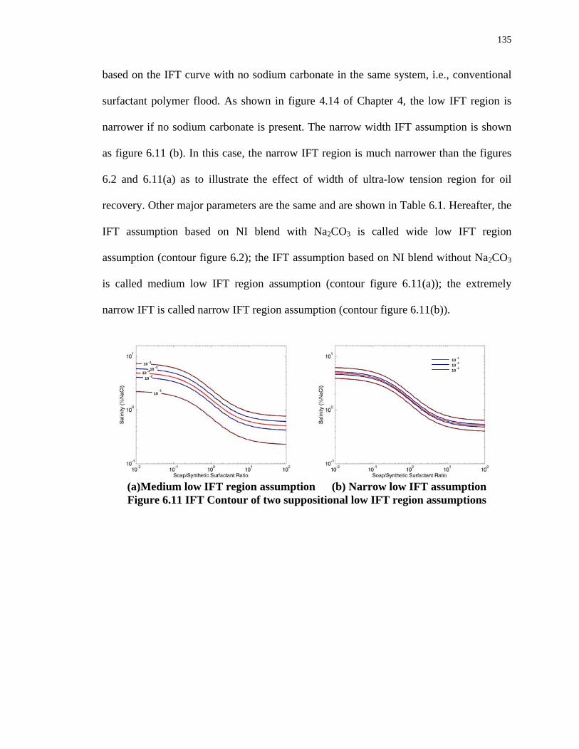
135

based on the IFT curve with no sodium carbonate in the same system, i.e., conventional

surfactant polymer flood. As shown in figure 4.14 of Chapter 4, the low IFT region is

narrower if no sodium carbonate is present. The narrow width IFT assumption is shown

as figure 6.11 (b). In this case, the narrow IFT region is much narrower than the figures

6.2 and 6.11(a) as to illustrate the effect of width of ultra-low tension region for oil

recovery. Other major parameters are the same and are shown in Table 6.1. Hereafter, the

IFT assumption based on NI blend with Na2CO3 is called wide low IFT region

assumption (contour figure 6.2); the IFT assumption based on NI blend without Na2CO3

is called medium low IFT region assumption (contour figure 6.11(a)); the extremely

narrow IFT is called narrow IFT region assumption (contour figure 6.11(b)).

1010

10

10

10-3-2

-2

-1

-1

1010 -2

10 -3

-1

(a)Medium low IFT region assumption (b) Narrow low IFT assumption Figure 6.11 IFT Contour of two suppositional low IFT region assumptions

136

1.E-03

1.E-02

1.E-01

1.E+00

0 1 2 3 4 5 6Salinity (% NaCl)

IFT

(mN

/m)

Simulation Curve (wide low IFT region)Simulation Curve (medium low IFT region)Simulation Curve (narrow low IFT region)

Soap to surfactant ratio =0.34

Figure 6.12 IFT simulation curves with different low IFT regions

Figure 6.12 shows the IFT versus salinity with different low IFT assumptions

when soap to surfactant ratio is 0.34. The minimum IFT value, i.e., the IFT values at

optimum are the same (10-3 mN/m). But the widths of low IFT region with different

assumptions are different.

The simulation results show that the recovery was 96% with wide low IFT region

and only 84% and 72% with medium and narrow low IFT region respectively. This result

can be explained by figure 6.13. The plots at left show the surfactant, soap, IFT, soap to

surfactant ratio and oil saturation profiles respectively for the wide low IFT region when

the dimensionless time equals 0.5 PV. The plots in the middle and at right show the same

profiles at same time but with medium and narrow IFT region. The width of the low

tension region (<10-2 mN/m) in the left profile is around 0.1 dimensionless distance,

while that of the low tension region in the right profile is only 0.03 dimensionless

distance. The oil saturation in the left profile is much less than that in the right profile.

Narrow low IFT region will have less recovery because oil is trapped when the IFT

increases. When the low IFT region is wide, less oil is trapped after the low tension

137

region. Thus, with the wide low IFT region in the alkali-surfactant system, higher oil

recovery can be achieved for a larger range of salinities. High salinities can cause

polymer-surfactant phase separation and lead to high surfactant and/or polymer retention.

With the wide low tension region and soap to surfactant gradient, high recovery can be

achieved by injecting at salinities well below the optimal value for the synthetic

surfactant such that the surfactant and polymer will coexist in the same phase.

Recovery=72%Recovery=96%

Narrow low IFT regionWide low IFT region

(NI blend with Na2CO3) Recovery=84%

Medium low IFT region (NI blend w/o Na2CO3)

Figure 6.13 Comparison of profiles between different low IFT region

assumptions

Another interesting phenomenon is the soap and surfactant concentration peak at

surfactant front when the IFT region is narrow. The generation of this peak is due to the

soap to surfactant gradient. As discussed in the previous section, soap and surfactant

ahead of low IFT region are retarded, while soap and surfactant behind the low IFT

138

region move forward with the velocity of aqueous phase. The accumulation of soap and

surfactant makes this peak. This effect is more significant when there is more trapped oil,

e.g., the narrow IFT case. Therefore, the displacement front of the ASP is a self-

sharpening process similar to the salinity gradient (Hirasaki et al., 1983). However, the

back of the surfactant slug can be a spreading wave.

6.2.3 Injection Solution Viscosity

Another factor for ASP is the injection solution viscosity. As figure 6.14 shows,

the injection solution viscosity can change the oil recovery significantly. The wide low

tension region was used in the two cases of figure 6.14. All major parameters except the

injection solution viscosity are the same as shown in Table 6.1. The plots in 6.14 show

the surfactant, soap, IFT, soap to surfactant ratio and oil saturation profiles respectively

when the dimensionless time equals 0.5 PV as in figure 6.13. The difference between

these plots is that the left plots are calculated by using 40 cp as the injection solution

viscosity, while the right plots use 24 cp as the injection solution viscosity.

The IFT profiles of these two conditions are similar to each other. However, the

oil saturation profiles are different, thus the oil recoveries are different. The injection

solution viscosity has a significant effect on recovery because it is related to mobility

ratio. Because the oil fractional flow increases with increasing aqueous phase viscosity,

the oil in the low tension region can be displaced in less distance before the IFT increases.

139

injecting solution viscosity=24cpinjecting solution viscosity=40cpRecovery =95% Recovery =86%

Figure 6.14 Comparison of profiles between varied injecting solution viscosities

Figure 6.15 illustrates this effect. Lower aqueous phase viscosity, i.e., higher

mobility ratio, has lower oil recovery even with wide low IFT region because it takes a

greater distance to displace the oil before the IFT increases. Thus, the injection solution

viscosity should be high enough to obtain high oil recovery. The fractional flow curve in

Figure 6.15 indicates that the displacement front should be a shock. However, the

simulation model includes dispersion. A self-sharping wave in the presence of dispersion

is not a shock but rather a wave of constant width (Pope, Lake and Helfferich, 1978)

140

Figure 6.15 Oil Fractional Flow vs. Saturation at IFT=0.001dyne/cm

(Oil viscosity =19.7 cp)

6.2.4 Effect of Dispersion

In the previous section, a Peclet number of 500 was chosen by matching the 1-D

sand pack adsorption experiments. However, the dispersion can be much larger, i.e., the

Peclet number can be much smaller, in the field due to the reservoir heterogeneity than

the 1-D sand experiments. Figure 6.16 shows the effect of dispersion for large surfactant

slug size.

141

Recovery=95%Recovery=96%Peclet No. = 500 Peclet No. = 50

Figure 6.16 Comparison of profiles between dispersions after 0.5 PV with large

surfactant slug (0.5PV)

The plots in 6.16 show the surfactant, soap, IFT, soap to surfactant ratio and oil

saturation profiles respectively when the dimensionless time equals 0.5 PV as in figure

6.13. The difference between these plots is that the left figures are calculated with Peclet

number 500, while the right figures use Peclet number 50. Peclet number 50 is chosen

because it represents the field scale dispersion for a distance of 1 km (Lake, 1989).

Because of the larger dispersion, the concentration profiles of the case with Peclet

number 50 change more gradually than the profiles of the case with Peclet number 500.

The surfactant front travels even faster and there is a longer soap concentration tail after

the surfactant front due to the high dispersion. This effect causes the soap to surfactant

142

ratio to change more gradually, so that the low IFT area in the profiles is even wider even

though the same low tension versus salinity relationship was used in both simulations.

This counteracts the effect of larger dispersion which may be expected to reduce the oil

recovery. The two cases have similar oil recovery. Therefore, the self-sharpening effect

of ASP helps to counteract the unfavorable larger dispersion when surfactant slug size is

large.

Recovery=57%Recovery=96%Peclet No. = 500 Peclet No. = 50

Figure 6.17 Comparison of profiles between dispersions with small surfactant

slug (0.2PV)

As shown in figure 6.17, the recovery factor changes much with dispersion when

the surfactant slug size is as small as 0.2 PV. From 6.17, the displacement front travels

slower when dispersion is large. Figure 6.18 is the distance-time diagram that illustrates

143

the difference between large and small surfactant slug. When surfactant slug size is large

(0.5 PV), the displacement front propagates at similar velocities with different dispersion.

However, when surfactant slug is small (0.2 PV), the displacement front seems not to

propagates any more after 0.3 PV with large dispersion. It is because the surfactant

concentration in the surfactant slug decreases significantly with large dispersion and

small surfactant slug. This makes the local soap to surfactant ratio larger so that more

surfactant partitions into the oleic phase and is retarded. In the section 6.2.6, the recovery

can be significantly improved by using salinity gradient.

Distance_Time Diagram

00.10.20.30.40.50.60.70.80.9

1

0 0.2 0.4 0.6 0.8 1 1.2 1.4T (PV)

X

Displacement Front 0.2 PV Surfactant, Pe=500) Unit Slope after 0.2 PVDisplacement Front (0.5 PV Surfactant, Pe=500) Unit Slope after 0.5 PVDisplacement Front (0.5 PV Surfactant, Pe=50) Unit SlopeDisplacement Front (0.2 PV surfactant, Pe=50)

Figure 6.18 Distance Time Diagram for different surfactant slug and dispersion

6.2.5 Optimum Operational Region

As shown in the previous section, the soap to surfactant ratio gradient in ASP

process assures that the process passes the optimum condition at the displacement front if

144

the injection salinity is between that of soap and surfactant. But that does not mean high

recovery can be achieved by injecting at any salinity between optimum salinity of soap

and surfactant for any conditions. A number of simulations were conducted with

different naphthenic soap concentrations, injected surfactant concentrations and salinity

(Appendix B). As figure 6.19 shows, the percent recovery of the waterflood residual oil

was contour plotted as a function of a characteristic soap fraction at the surfactant front as

abscissa and the injected dimensionless salinity as the ordinate. To make the contour plot

consistent, the recovery efficiency is the oil recovery at 2.0 pore volumes. The soap

fraction at the surfactant front and dimensionless salinity are defined as equation (6.16)

and (6.17). The soap fraction is volume of soap in an element of pore volume at initial Sor

as a fraction of surfactant plus soap if the initial brine is replaced by surfactant solution to

be injected.

)1(**

*_

orsurfactantorsoap

orsoap

SCSCSC

FractionSoap−+

= (6.16)

where Csoap is the soap molar concentration. KOHMWNoAcidCsoap _/._=

Sor is initial oil saturation,

Csurfactant is injection surfactant molar concentration,

SoapofSalinityOptimumSalinitySalinityessDimensionl

____ = (6.17)

Since the optimum salinity of pure soap in this case is 0.5% NaCl, the value of

dimensionless optimum salinity of pure surfactant is 10 because optimum salinity of pure

surfactant is 5% NaCl.

145

6.2.5.2 Wide low tension assumption with 0.5 Pore Volume Surfactant Slug

90%

70%

50%

30%

Optimum Curve

30%

50%70%

90%

Acid No.=0.2mg/g, surfactant concentration=0.14%, salinity=1.0% NaCl (figure 6.20)



Figure 6.19 Contour of recovery factor at 2.0 PV with 0.5 PV surfactant slug size

(wide low IFT assumption)

From figure 6.19 in which the surfactant slug size is 0.5 pore volume with wide

low IFT assumption, high oil recovery can be achieved by following the optimum curve

which is determined by the phase behavior experiments. The optimum salinity line on the

plot is that for characteristic soap fraction based on figure 3.10 that gives optimum

conditions. When the injected salinity is more than the calculated optimum salinity, the

recovery factor will drop off very quickly when the salinity reaches a certain high value.

This is because of surfactant retardation and retention with over-optimum conditions.

146

Nearly all the surfactant is trapped in the oil phase and will not propagate any more. The

recovery efficiency falls off more gradually when the injected salinity is less than the

calculated optimum salinity.

Figure 6.20 Profiles for an under-optimum case with 0.5 PV surfactant slug size

wide low tension assumption (Acid No.=0.2mg/g, surfactant concentration=0.14%, injection salinity=1.0%)

Figure 6.20 shows the typical profiles for the under-optimum case at time 0.5 and

1.0 pore volume after initial injection for a 0.5 PV surfactant slug size with wide low IFT

147

assumption. This case is with 0.2 mg/g acid number, 0.14% surfactant so that the soap

fraction for this case is 0.42, for which the dimensionless optimum salinity is 3.8, or the

optimum salinity is 1.9 % NaCl. The injection salinity for figure 6.20 is 1.0 % NaCl so

that it is an under-optimum case as shown as the green point in figure 6.19. The recovery

efficiency for this condition is 89.5%.

Similar to the base case profiles, the soap front is ahead of the surfactant, and a

soap to surfactant gradient is generated during this ASP process in figure 6.20. The IFT

value is high at the soap front (where soap is generated) because of the over-optimum

condition; it is also very high at the rear of the surfactant slug because it is under-

optimum. There is a low IFT optimum region which displaces the oil. The lowest tension

is located at the optimum soap to surfactant ratio when salinity is 1% NaCl. The profiles

in figure 6.20 indicate that 0.5 PV surfactant slug size is larger than needed. The

surfactant profile shows that there is still a lot of surfactant present behind the IFT

minimum. However, IFT in this region is too high to displace the oil remaining there.

Figure 6.21 shows the same case as that in figure 6.20 except the injection salinity

is 2.0% NaCl which is near the optimum curve. The recovery efficiency for this condition

is 98.1%. The concentration and IFT profiles are similar to the under-optimum case, and

the slug again is much larger than needed. The IFT value (~0.02 mN/m) in the surfactant

slug in this case is lower than that (0.1mN/m) in under-optimum cases. The reason that

optimum condition has a higher recovery is because it has moderately low IFT at the

injection point (XD=0). Figures 6.20 and 6.21 show that the recovery efficiency does not

change much in going from optimum to under-optimum conditions.

148

Figure 6.21 Profiles for an optimum case with 0.5 PV slug size and wide low

tension assumption (Acid No.=0.2mg/g, surfactant concentration=0.14%, injection salinity=2.0%)

Figure 6.22 shows the over-optimum case with injection salinity 4.0 % NaCl. The

recovery efficiency is 100% after 2.0 PV. The low propagation velocity of low tension

region is because the higher salinity results in higher partition coefficient and thus slower

surfactant propagation. This is typically seen in the over-optimum surfactant flood

(Nelson, 1978). Although it shows higher recovery in this case, it may not desirable due

149

to large surfactant slug required (0.5 PV). When the surfactant slug becomes less, the

recovery will drop significantly, (see small slug results in the next section). The effect of

surfactant-polymer phase separation was not modeled. This effect could have made the

over-optimum case much worse.

Figure 6.22 Profiles for an over-optimum case with 0.5 PV slug size and wide low


150

6.2.5.2 Wide low tension assumption with 0.2 Pore Volume Surfactant Slug

If the surfactant slug size is reduced to 0.2 pore volumes, the recovery contour

plot is shown as figure 6.23. Compared to figure 6.19, the contour shape in the under-

optimum part does not change much but that in the over-optimum part changes a lot. This

effect can be explained by figures 6.24, 6.25 and 6.26, which are the counterparts of

figures 6.20 to figure 6.22 but with smaller slug size`.

90%

70%

50%

30%

Optimum Curve

30%50%70%

90%





(wide low tension assumption)

The under-optimum conditions in figure 6.24 are the same as that of figure 6.20

except the surfactant slug size is 0.2 pore volume. The recovery factor for this condition

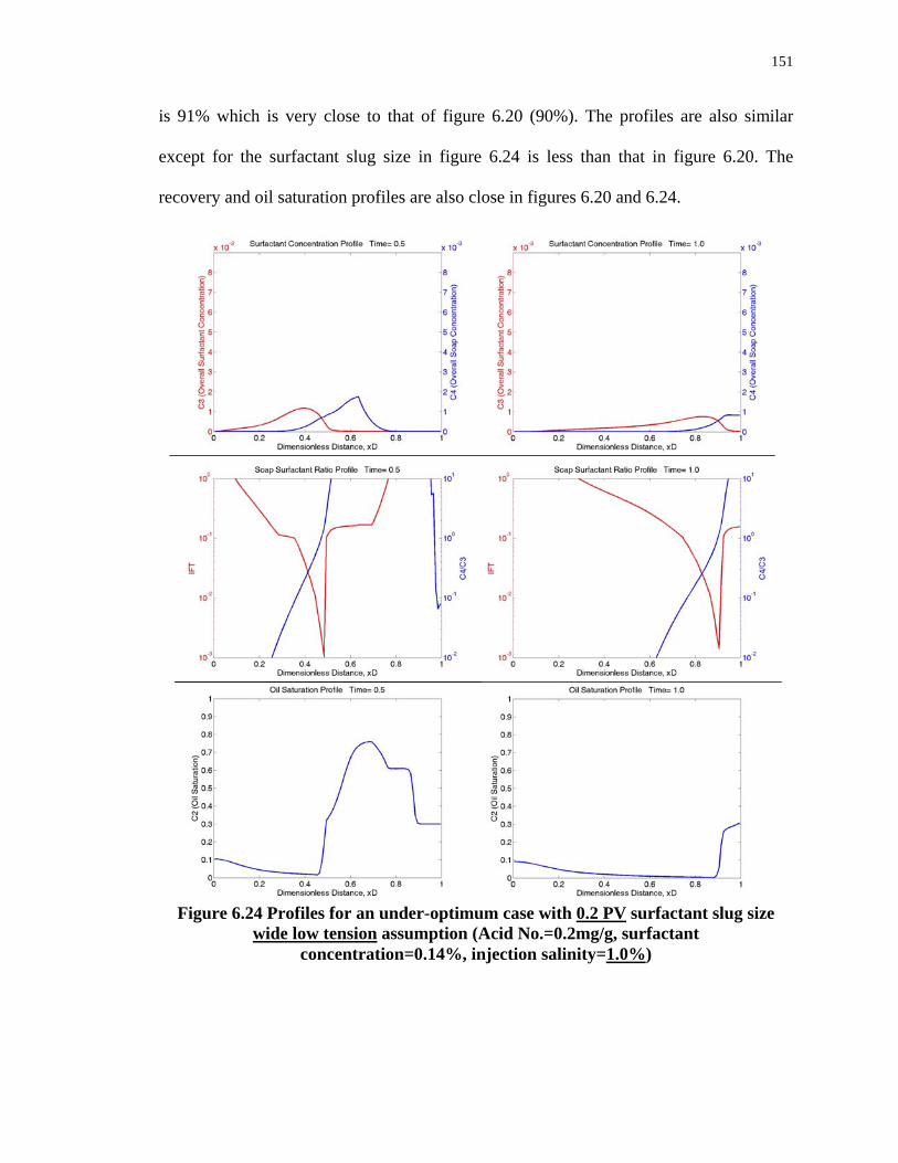
151

is 91% which is very close to that of figure 6.20 (90%). The profiles are also similar

except for the surfactant slug size in figure 6.24 is less than that in figure 6.20. The

recovery and oil saturation profiles are also close in figures 6.20 and 6.24.

Figure 6.24 Profiles for an under-optimum case with 0.2 PV surfactant slug size

wide low tension assumption (Acid No.=0.2mg/g, surfactant concentration=0.14%, injection salinity=1.0%)

152

Figure 6.25 with 0.2 PV surfactant slug near optimum is the counterpart to figure

6.21 with 0.5 PV surfactant slug for the optimum condition (2% NaCl). The recovery

factor for figure 6.25 is 98.4% while that for figure 6.20 is 98.1%. Similar to the under-

optimum cases, the slug size does not change the recovery much.

Figure 6.25 Profiles for a near optimum case with 0.2 PV slug size and wide low


153

Figure 6.26 Profiles for an over-optimum case with 0.2 PV slug size and wide low


For over-optimum case with 4% NaCl, the recovery changes much as shown in

Fig. 6.26. The case with 0.2 pore volume surfactant slug shown in figure 6.26 has only

62.6% oil recovery. Compared to figure 6.22, the surfactant travels much slower with 0.2

PV surfactant slug than with 0.5 PV slug. At time equals 1.0 pore volume after injection,

the surfactant front is only at XD=0.5, while in 0.5 PV surfactant slug case, the surfactant

154

front is at XD=0.7. This is because soap and surfactant is trapped in the oil phase when at

over-optimum case and with a small slug, there is not enough surfactant to lower the soap

to surfactant ratio enough to transfer the soap and surfactant into the aqueous phase. With

a small slug and constant salinity, it’s better to operate the ASP process at or slightly

below the optimum salinity as calculated by the soap fraction. Below optimum condition,

surfactant retardation and retention is less a problem and interfacial tension remains

moderately low valued in the Winsor I conditions because of the presence of naphthenic

soap. As a result, the recovery will stay high and change more gradually with salinity. If

the salinity is not constant, i.e. a salinity gradient is used, the recovery can be improved.

This will be further discussed in section 6.26.

It is possible for someone to design with over-optimum conditions if a large

water/oil ratio is used to determine optimum salinity. The results here suggest that the

injection salinity should be designed using water/oil ratio corresponding to (1-Sor)/Sor.

6.2.5.3 Narrow low tension assumption with 0.5 & 0.2 Pore Volume Surfactant Slug

As discussed in section 6.2.2, the width of low tension region changes the

recovery significantly. However, the wide low tension might not be general; at least it is

not valid for zero soap condition. Figure 6.27 and figure 6.28 plot the recovery contours

for the case with narrow low tension assumption for 0.5 pore volume and 0.2 pore

volume surfactant slug respectively.

155

70%50%

30%

Optimum Curve 30%

50%70%

90%

90%


(narrow low tension assumption)

70%

50%

30%

Optimum Curve

30%

50%

70%

90%

90%


(narrow low tension assumption)

156

It seems that high recovery is reached at optimum salinity of soap with pure soap

or at optimum salinity or surfactant with pure surfactant. These results are reasonable

because they are either alkali flood (soap fraction=1.0) or surfactant flood (soap

fraction=0) at their exact optimum condition. In the other area, moderately high recovery

(>70%) can be achieved by following the optimum curve line. Higher recovery can be

achieved by increasing the injection fluid viscosity as discussed in section 6.2.3 because

it allows more oil to be displaced by highly viscous water before the IFT increases.

However, it will increase the cost and reduce the injectivity for the reservoir applications.

From figure 6.27, high recovery can also be achieved at salinity close to the

optimum salinity of surfactant by using 0.5 pore volume surfactant slug size with low

soap fraction number. This can be explained by figure 6.29, which compares the profiles

with 0.2 and 0.5 pore volume surfactant slug sizes. Other conditions, such as acid number

and surfactant concentration, salinity, are the same. The injection salinity is exactly at

optimum salinity of surfactant (5.0% NaCl). From figure 6.28, the ultra low tension can

be achieved when soap is displaced and surfactant is dominant. In this case, the width of

low tension region will not affect the low tension width in the reservoir since the

reservoir salinity is at the optimum salinity of surfactant. The upper right region with

90% oil recovery in contour figure 6.29 can be regarded as the transition area from

surfactant process to ASP process. For the ASP process with very low acid component or

very high surfactant concentration, it is similar to traditional surfactant process and

should be operated at the optimum condition of surfactant if salinity is to be maintained

constant as in this study. But if the ASP process is operated at this condition, operator

157

should aware that the surfactant propagation rate is very slow and it works only with

large surfactant slug.

0.2 PV surfactant slug (recovery=30%) 0.5 PV surfactant slug (recovery=88%) Figure 6.29 Comparison of slug size with narrow low tension assumption (Acid

No.=0.2mg/g, surfactant concentration=0.14%, injection salinity=5.0%)

158

6.2.6 Salinity Gradient in ASP

Previous sections in this chapter show the constant salinity cases. In this section,

the benefit of the salinity gradient will be shown.

6.2.6.1 Salinity Gradient for Large Dispersion and Small Surfactant Slug

As discussed in section 6.2.4, large dispersion and small surfactant slug causes

low recovery with constant salinity. As shown in figure 6.17 and 6.18, the displacement

front of large dispersion and small surfactant slug is significantly retarded so that the

recovery is poor. To improve the recovery, a salinity gradient is applied. In this salinity

gradient case, the initial salinity is 4% NaCl, the salinity in the 0.2 PV surfactant slug is

2% and the drive salinity is 1% NaCl. It is found that the recovery of the salinity gradient

case is 98% even with large dispersion (Pe=50), while the recovery of constant salinity is

only 57% with large dispersion. Figure 6.30 compares the profiles of the constant salinity

(2% NaCl) and this salinity gradient design with large dispersion. Although the surfactant

and soap profiles look similar, the displacement front of the salinity gradient case is faster

than that of the constant salinity. This is because more soap and surfactant partition into

aqueous phase with low salinity at the same soap to surfactant ratio. In addition to the

soap to surfactant ratio gradient, the salinity gradient further improves the recovery.

159

Salinity gradient Constant salinity (2% NaCl)Recovery = 98% Recovery = 57%

Figure 6.30 Comparison of salinity gradient and constant salinity with large

dispersion

Figure 6.31 is the distance-time diagram for the salinity gradient case and

constant salinity case. Figure 6.31 shows that the displacement front sweeps the whole

area and recovers almost all the oil with the salinity gradient, while the displacement

front of constant salinity stops propagating after 0.3 PV such that the recovery is poor.

160

Distance_Time Diagram for small surfactant slug and large dispersion

00.10.20.30.40.50.60.70.80.9

1

0 0.2 0.4 0.6 0.8 1 1.2 1.4 1.6T (PV)

X

Unit SlopeDisplacement Front (0.2 PV Surfactant slug with salinity gradient)Displacement Front (0.2 PV surfactant with constant salinity)Unit Slope after 0.2 PV

Figure 6.31 Distance-time diagrams of salinity gradient and constant salinity with

large dispersion (Pe=50)

6.2.6.2 Salinity Gradient for Over-optimum 0.2 PV surfactant with Small Dispersion

The poor recovery of the over-optimum case shown in figure 6.26 can also

improved by this salinity gradient. For the over-optimum case with constant 4% NaCl,

the recovery is only 63%. If a low salinity (1% NaCl) drive, rather than the 4% NaCl, is

injected. The recovery is improved to 99.5%. The profiles of the constant salinity over-

optimum case and the salinity gradient case are shown in figure 6.32. Figure 6.33 is the

distance time diagrams. Figure 6.33 shows that salinity gradient makes the displacement

front travel fast so that it can propagates through the reservoir, while the displacement

front of constant salinity of over-optimum case is retarded and stops propagation after 1

PV. Figure 6.33 also shows the reason that large surfactant slug of over-optimum case

can give the good recovery. It is because large surfactant slug keeps the drive front away

from the displacement front so that the displacement front can sweep the whole reservoir.

161

Small surfactant slug (0.2 PV)Salinity Gradient =4% NaCl +1% NaCl drive

Recovery=99.5%Recovery=63%

Small surfactant slug (0.2 PV)Constant Salinity =4% NaCl

Figure 6.32 Comparison of salinity gradient and constant salinity for small

surfactant slug at over-optimum condition (small dispersion)

Distance_Time Diagram

0

0.1

0.2

0.3

0.4

0.5

0.6

0.7

0.8

0.9

1

0 0.2 0.4 0.6 0.8 1 1.2 1.4T (PV)

X

Unit Slope

Displacement Front (0.5 PV Slug, constant salinity, 4% NaCl) Drive front with Unit Slope (0.5 PV slug)

Displacement Front (0.2 PV Slug, constant, Salinity, 4% NaCl)

Displacement Front (0.2 PV Slug with salinty gradient, 4 1% NaCl)

Drive front with Unit Slope (0.2 PV slug)

Drive front with Unit Slope (0.2 PV slug) Figure 6.33 Distance-time diagrams of salinity gradient and constant salinity for

over-optimum conditions (small dispersion)

162

6.2.7 Summary of Simulations

The simulation shows a soap to surfactant ratio gradient is generated in the ASP

process. This gradient not only assures the profile of passing through the optimal

condition where the low IFT is achieved, but also makes ASP a robust process because

surfactant that moves ahead into the soap-dominant region ahead of the major surfactant

bank is retarded and surfactant behind the displacement front travels at the velocity close

to the aqueous phase.

Narrow low IFT region will have less recovery because oil will be trapped again

when the IFT increases. When the low IFT region is as wide as the experimental values

for Yates oil and NI blend, less oil will be trapped after the low tension region. Thus, it is

favorable to have the ASP formulation with wide low IFT region.

The injection solution viscosity has significant effect on recovery. Lower aqueous

phase viscosity, i.e., higher mobility ratio, has lower oil recovery even with wide low IFT

region. It is because oil fractional flow is less even in the low IFT region where the

residual oil saturation is zero. Oil will be trapped again after the low tension region.

There is an optimum operation region for ASP process, which can be determined

if the initial natural soap content is known. For a certain surfactant concentration, good

recovery can be achieved in a certain range of salinity which follows the relationship of

optimum salinity and soap to surfactant ratio.

With significant dispersion, the recovery for small surfactant slug may be

significantly less than that for the large surfactant slug, even at optimum conditions.

With salinity gradient, ASP process could work well with small surfactant slug

and large dispersion.

163

Chapter 7

Alkali Surfactant Polymer Flooding

Based on the phase behavior, IFT, adsorption and simulation results, ASP

flooding experiments were designed. Results are presented in this chapter. The flooding

experiments can be used to demonstrate those important mechanisms that have been

identified and incorporated in the simulator in previous chapters and provide the

directions for the real field test.

7.1 Flooding Experimental Procedure

The ASP solution used in the flooding experiments is the NI blend and the

polymer (polyacrylamide, CS 3330® from SNF Inc.). The general mixing procedure for

ASP solution is as follows:

1. Mix sodium chloride and sodium carbonate with DI water

2. Add surfactant into solution before adding polymer.

3. Using the magnetic stirrer, establish a vortex in the surfactant solution in step 2 that

just reaches the stir bar. Sprinkle the desiccated polymer powder on the shoulder of

the vortex just slowly enough to prevent clumping of the polymer. Adding the

polymer too fast will form gel which is very difficult to dissolve.

164

4. Continue stirring the polymer solution until all polymer particles appear to be fully

hydrated and dissolved. This may take 30-60 minutes. Visual examination should

show that no turbity exists. Continue stirring for an additional 30 minutes to let the

solution hydrate.

The flooding experimental apparatus shown in figure 7.1 is similar to what is used

in dynamic surfactant adsorption experiments except the pump is the HPLC pump

(ISCO® Model 2350) because high injection pressure is needed due to the high viscosity

fluids. The other difference is that the one foot long sand pack is vertical so that the

gravity will help to stabilize the oil-brine interface.

The ASP flooding experiments were conducted by the following procedure:

1. CO2 was injected into the sand pack so that it was saturated with CO2 with no air left.

2. Brine with 2% NaCl was injected at the velocity 0.5 ml/min (interstitial velocity = 14

ft/day) until the column was saturated by the brine. The objectives of step 1 and 2 is

to eliminate the air that will be trapped in the column

3. Crude oil was injected at the velocity 0.5 ml/min (interstitial velocity = 14 ft/day)

until the oil broke through.

4. The oil-saturated column was placed into a 60 °C oven for 60 hours. The purpose of

this aging procedure was to change the wettabilty of the substrate (dolomite) to

mixed-wet.

5. After aging, brine with 2 % NaCl was pumped into the column at velocity 0.5 ml/min

(interstitial velocity = 14 ft/day) until there was no oil in the effluent.

6. The ASP solution is injected at velocity around 1 ft/day.

165

HPLC Pump

1-d column

Computer

(Monitoring pressure)

Sample Collection

Figure 7.1 Schematic Experimental Apparatus for flooding

7.2 Alkaline Surfactant Polymer Flooding for Yates Oil

The ASP flooding for Yates oil was performed on a 35 darcy dolomite sand (from

Unimin Corp.) pack. Figure 7.2 shows the photos for Yates oil flooding and water

flooding before the ASP flooding. the left one in figure 7.2 is the oil flooding after 0.1

Pore Volume (PV). The oil cut was 100% immediately after breakthrough. The oil

saturation after the oil flooding was 0.98. The right five photos illustrate the water

flooding at different pore volumes injected. The cumulative oil recovery and the

fractional flow of oil at the outlet are shown in figure 7.3. In this figure, the oil saturation

is 0.177 (Sor=0.177) after 3.2PV was injected. Further injection of water would not be

expected to recover much more oil.

166

Oil Flooding Water Flooding

Aged in 60ºC for 60 hours

0.1PV 0.3PV 0.5PV 1.0 PV 2.0PV 3.0PV Figure 7.2 Oil flooding and water flooding for Yates oil

Water flooding

0.00.10.20.30.40.50.60.70.80.91.0

0.0 0.5 1.0 1.5 2.0 2.5 3.0 3.5

Pore Volumes

Cum

ulat

ive

Oil

Rec

over

y/ O

OIP

0.00.10.20.30.40.50.60.70.80.91.0

Oil

Cut

Cumulative Oil Recovery Oil Cut

Figure 7.3 Oil Recovery of Water Flooding in Dolomite Sand Pack (OOIP: Original Oil in Place)

After water-flooding, ASP process was implemented on the dolomite sand pack.

A 0.50 PV slug of ASP solution was injected into the sand pack followed by a 1.0 PV

167

polymer drive. The formulation of alkaline-surfactant-polymer solution is shown in Table

7.1. The viscosity of ASP solution was 45.1 cp at the shear rate of 66 sec-1. The reason

that such high viscosity was used is that the crude oil viscosity was 19.4 cp. The polymer

drive consists of 5000 ppm polymer and 2.0% NaCl.

Chemicals Concentration Alkali (Na2CO3) 1.0 %

NaCl 2.0% Surfactant (NI Blend ) 0.2%

Polymer (Flopaam 3330) 5000ppm

Table 7.1 Formulation for ASP solution for Yates oil flooding

0.05 0.10 0.15 0.20 0.25 0.30 0.35 0.40 0.45 0.50 0.55 0.60 0.65 0.70 0.75 0.90 1.50

Injecting Pore Volumes

Figure 7.4 Photos of ASP flooding for Yates in dolomite pack at different injecting pore volumes

The photos in figure 7.4 represent how the oil bank forms and propagates during

the ASP process. Figure 7.5 shows the cumulative oil recovery and the fractional flow of

produced oil. And the effluent of the flooding at different pore volumes is shown in

figure 7.6. The oil bank breaks though at 0.8 PV. The surfactant breaks through at around

168

0.99 PV because lower phase micro-emulsion can be found at that time. The incremental

oil recovery is 98.1% and the oil recovery without emulsion is 61.3%. There may be

some oil in the aqueous phase because the color of the aqueous phase of some effluent is

brown.

0.0

0.2

0.4

0.6

0.8

1.0

0.0 0.2 0.4 0.6 0.8 1.0 1.2 1.4 1.6 1.8 2.0

Pore Volumes

Incr

emen

tal O

il .

Rec

over

y/R

OIP

0.0

0.2

0.4

0.6

0.8

1.0

Oil

Cut


SurfactantSlug

PolymerDrive

SurfactantBreakthrough

Figure 7.5 Oil Recovery of ASP Flooding for Yates oil in Dolomite Sand Pack

(ROIP: Residual Oil in place)

0.09 0.27 0.45 0.63 0.81 0.99 1.17 1.35 1.53 1.71 1.89 2.070.18 0.36 0.54 0.72 0.90 1.08 1.26 1.44 1.62 1.80 1.98

Effluent Pore Volumes0.09 0.27 0.45 0.63 0.81 0.99 1.17 1.35 1.53 1.71 1.89 2.07

0.18 0.36 0.54 0.72 0.90 1.08 1.26 1.44 1.62 1.80 1.98

Effluent Pore Volumes

Figure 7.6 Effluent of ASP Flooding in Dolomite Sand Pack

The history of pressure drop is shown in figure 7.7. The pressure increases with

the injection because the surfactant slug and polymer drive were designed to have a

169

favorable mobility ratio. The pressure became stable and did not increase any more after

the surfactant broke through because the whole column was occupied by the surfactant

slug and polymer drive which have nearly identical viscosities. Further injecting polymer

solution did not change the apparent viscosity of the system.

0

0.5

1

1.5

2

2.5

3

3.5

0 0.2 0.4 0.6 0.8 1 1.2 1.4 1.6

Pore Volume (PV)

Pres

sure

diff

eren

ce (p

si)

Surfactant Slug

Polymer Drive

Surfactant Breakthrough

Figure 7.7 Pressure drop during ASP flood for Yates oil in dolomite sand pack.

The one-dimensional simulator described in Chapter 6 was used to simulate this

experiment. Figure 7.8 compares the simulation results and the experimental results. This

plot shows the simulation result matches the experimental results quite well.

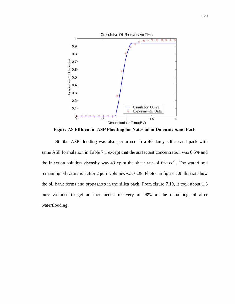
170

Figure 7.8 Effluent of ASP Flooding for Yates oil in Dolomite Sand Pack

Similar ASP flooding was also performed in a 40 darcy silica sand pack with

same ASP formulation in Table 7.1 except that the surfactant concentration was 0.5% and

the injection solution viscosity was 43 cp at the shear rate of 66 sec-1. The waterflood

remaining oil saturation after 2 pore volumes was 0.25. Photos in figure 7.9 illustrate how

the oil bank forms and propagates in the silica pack. From figure 7.10, it took about 1.3

pore volumes to get an incremental recovery of 98% of the remaining oil after

waterflooding.

171

Figure 7.9 Photos of ASP flooding for Yates oil in silica pack at different injecting pore volumes

0.0

0.2

0.4

0.6

0.8

1.0

0.0 0.2 0.4 0.6 0.8 1.0 1.2 1.4 1.6Pore Volumes

Incr

emen

tal O

il

Rec

over

y/R

OIP

0.0

0.2

0.4

0.6

0.8

1.0

Oil

Cut


SurfactantSlug

PolymerDrive

SurfactantBreakthrough

Figure 7.10 Oil Recovery of ASP Flooding for Yates oil in Silica Sand Pack


The pressure drop history is shown as figure 7.11, in which the final pressure drop

is close to that of figure 7.7. Figure 7.12 also shows that the simulation result matches the

172

experimental results with the exception of the early oil production. The early oil

breakthrough in this experiment is because the remaining oil saturation after

waterflooding is slightly greater than the residual oil saturation after water flooding.

0

0.5

1

1.5

2

2.5

3

3.5

0 0.2 0.4 0.6 0.8 1 1.2 1.4 1.6

Pore Volume

Pres

sure

diff

eren

ce (p

si)

Surfactant Slug

Polymer Drive


Figure 7.11 Pressure drop during ASP flood for Yates oil in silica sand pack.

Figure 7.12 Effluent of ASP Flooding for Yates oil in silica sand pack

173

7.3 The Problem of Phase Separation of Injection Solution

The phase behavior experiments of NI blend and Yates oil show that the optimal

salinity for NI blend and Yates is around 5% NaCl with 1% Na2CO3 without the presence

of soap. If an experiment was run at salinity close to the optimal salinity of NI blend

itself, the recovery might be even better than with the previous 2% NaCl, according to the

phase behavior experiments without presence of polymer.

0 PV 0 .17 PV 0 .33 PV 0 .5 PV 0 .67 PV 0 .83 PV 1 .0PV 2 .0 PV Figure 7.13 Photos showing behavior during unsuccessful ASP flood of silica sand

pack where phase separation due to polymer has occurred.

Another ASP flooding was done at the same condition as in figure 7.9 except the

injection salinity was 4.0% NaCl. Before injection, the ASP solution with 4% NaCl

looked a bit turbid while the 2% NaCl ASP solution was clear. As figure 7.13 shows, no

distinct oil bank was found after injection. There is significant amount of oil that

propagated behind surfactant front. The mobilized oil appears to be behind the surfactant

front as if there was lack of mobility control.

174

0

5

10

15

20

25

30

0 0.5 1 1.5

Pore Volume

Pres

sure

Diff

eren

ce (p

si

2

)Surfactant Slug Polymer Drive


Figure 7.14 Pressure drop during ASP flood in silica sand pack where phase

separation due to polymer has occurred.

Moreover, the pressure drop shown in figure 7.14 indicates that the pressure drop

rose to 25 psi, which was around 10 times of that in figure 7.11. This implies that there is

a more viscous phase in the experiment of figure 7.13 since the flow rates were same in

both experiments. After one week settling of the ASP solutions with different salinities,

phase separation can be observed in the sample with 4% NaCl, as seen in the right figure

in Figure 7.15. There is a separated layer in that sample. This separated layer must be a

highly viscous polymer-rich phase that caused the high pressure drop. Before the polymer

drive was injected, the highly viscous polymer-rich phase might adhere at the sand pack

entrance. The polymer-lean phase of newly injected ASP solution might have to break

past the polymer-rich gel so that the pressure drop sharply oscillated. After the polymer

drive was injected, the pressure drop significantly increased because the highly viscous

polymer-rich phase dissolve in the polymer drive due to absence of surfactant. Thus, the

175

injected solution should be a clear, one-phase system in ASP flooding system. Otherwise,

phase separation may occur during the flooding process. Lowering injection salinity

would be a good way to avoid the phase separation. This is one of the benefits of ASP

process. The flooding salinity does not need to be at the exact optimum salinity of

synthetic surfactant.

0.5% NI Blend

0.5% Flopaam 3330S,

2% NaCl, 1% Na2CO3

0.5% NI Blend

0.5% Flopaam 3330S,

4% NaCl, 1% Na2CO3

Separate layer

Figure 7.15 Phase separation caused by increasing NaCl content for aqueous

solution of 0.5 wt% NI blend, 1 wt% Na2CO3 and 0.5 wt% polymer.

7.4 Alkali Surfactant Flooding Process for High Viscosity Oil

It is very difficult to maintain a favorable mobility ratio for high viscosity oil, e.g.,

PBB oil (266cp). According to the simulation for highly viscous oil, the oil recovery will

be only around 40% even with 5000 ppm polymer. To recover this highly viscous oil,

mobility control method other than the polymer should be considered. An ASP

176

experiment with co-injection gas was performed on silica sand pack as shown in figure

7.16. The oil saturation initially in the column was 0.36 which is the remaining oil after 6

pore volume waterflooding. The ASP process started with 0.3 pore volume injection with

ASP solution (NIP: 0.5% NI blend and 5000 ppm polymer) at 1 ft/day as used for Yates

oil. The salinity is 1%NaCl with 1% Na2CO3. This salinity is chosen because there is

more soap in PBB than in the Yates oil so that the optimum injection salinity is lower as

shown in the Chapter 6. There is some oil displaced by the ASP solution. However, there

is still much oil left and no oil bank formed due to the unfavorable mobility ratio. After

0.3 pore volume, slugs of 0.1 pore volume air and 0.1 pore volume ASP solution were

alternately injected at 20 ft/day. Such a high injection rate is to maintain the pressure that

can generate strong foam (Yan, 2006). From figure 7.16, it is obvious that much trapped

oil was displaced by the alternate injection of air and ASP solution. After 0.8 PV, slugs of

0.1 pore volume air and 0.1 pore volume IOS solution (0.5% IOS, 1% NaCl, 1% Na2CO3)

were alternately injected at 20 ft/day. The IOS solution was chosen because IOS is a

strong foamer so that it will show high apparent viscosity and generate good mobility

ratio (Yan, 2006). Figure 7.16 indicates that the trapped oil continuously be displaced by

the foam drive even without using a polymer drive.

Figure 7.17 shows the oil broke through at 0.6 pore volume. An incremental

recovery of 93% of the remaining oil after waterflooding was reached at around 2.0 pore

volume. A certain amount of oil solubilized in the aqueous effluent was not measured and

not included in this recovery number. The actual recovery might be even higher. Figure

7.18 is the pressure history of this flooding. The highest pressure drop is around 2.5 psi.

177

NIP

0 0.05 0.1 0.15 0.2 0.3 0.4 0.5 0.6 0.7 0.8 0.9 1.0 1.1 1.2 1.3 1.4 1.5 1.6 1.7 1.8 2.0Injecting Pore Volumes

NIP: 0.5% NI, 5000ppm Polymer, 1% NaCl, 1% Na2CO3IOS: 0.5% IOS, 1% NaCl, 1% Na2CO3

NIP

1 foot/day

Air AirAir Air Air AirAir AirNIP IOS IOS IOS IOS IOS IOS

20 foot/day

Figure 7.16 Photos of ASP Foam flooding for PBB in silica pack at different injecting pore volumes.

0.0

0.1

0.2

0.3

0.4

0.5

0.6

0.7

0.8

0.9

1.0

0.0 0.2 0.4 0.6 0.8 1.0 1.2 1.4 1.6 1.8 2.0 2.2 2.4 2.6 2.8Pore Volumes

Cum

ulat

ive

Oil

Rec

over

y

0.0

0.1

0.2

0.3

0.4

0.5

0.6

0.7

0.8

0.9

1.0

Oil

Cut

Cumulative Oil Recovery Oil Cut Figure 7.17 Oil Recovery of ASP Foam Flooding for PBB oil in Silica Sand Pack


178

Pressure drop of ASPF flooding for PBB oil

0.0

0.5

1.0

1.5

2.0

2.5

3.0

0.0 0.1 0.2 0.3 0.4 0.5 0.6 0.7 0.8 0.9 1.0 1.1 1.2 1.3 1.4 1.5 1.6 1.7 1.8 1.9 2.0

Pore Volume (PV)

Pres

sure

diff

eren

ce (p

si)

NIP

NIP

1 foot/day

Air AirAir Air Air AirAir AirNIP IOS IOS IOS IOS IOS IOS

20 foot/daySurfactant- alternating-air

Figure 7.18 Pressure drop during ASP Foam flood for PBB oil in silica sand pack

This result shows that alternative injection of ASP solution and gas can recover

high viscosity oil that could not be recovered by ASP itself. The mechanisms of this

surfactant gas process are still not fully understood and need further study. One

speculation for the mechanism is shown at figure 7.19. The local pressure gradient ∇P at

the bubble front may be much greater than the average because the pressure difference in

the bubble (ΔPb) is quite small and the pressure drop along the bubble (ΔPL) will be

concentrated at the bubble front. Also the presence of IOS still significantly reduces the

interfacial tension although it is not as good as NI blends. Some foam studies (Yan, 2006,

Li, 2006) show that gas saturation can achieve very large values with surfactant than the

conditions without presence of surfactant. Since gas saturation becomes larger, it might

help to reduce the oil saturation. To verify those mechanisms, more studies are needed.

179

L

Flow direction

ΔPL

ΔPb≈ 0 ΔPb≈ 0

δ

LPPP LL Δ

>>Δ

≈∇δ

Figure 7.19 A possible mechanism for ASP foam process

180

Chapter 8

Conclusions and Future Work

In this chapter, the conclusions and recommendations for future work are

presented.

8.1 Conclusions

8.1.1 Phase Behaviors of Alkali-Surfactant System (Chapter 3)

Alkali can react with acids in crude oil to form natural soap, which acts as anionic

surfactant. However, natural soap usually is too hydrophobic and optimal salinity is very

low. The addition of synthetic surfactant can significantly increase the optimum salinity.

Alkaline surfactant phase behavior is a function of salinity, surfactant concentration, and

water oil ratio (WOR). The optimum salinity depends on soap to surfactant ratio for both

low acid number oil (Yates) and high acid number oil (PBB). However, the shape of the

optimum salinity curve depends on the oil and surfactant. Different oils and surfactants

may have different curves. With the acid number determined by soap extraction with

alkali, the mixing rule developed by Bourrel and Schechter for orthoxylene sulfonate

mixtures can be used to characterize the alkaline surfactant optimum salinity. This is

because soap extraction with alkali only measures the soaps that have surface active

properties. From the pure hydrocarbons phase behavior, the optimum salinity is also a

181

function of refined oil carbon number. Introducing SBA can change the optimum salinity.

For NI blend and Yates oil, birefringent material is observed in the microemulsion near

optimum salinity. However, it does not affect the viscosity of the microemulsion phase.

8.1.2 Interfacial Tension Properties of Alkali Surfactant System (Chapter 4)

Crude oils may be contaminated by emulsion breaker, scale inhibitor, or rust

inhibitor. Before any phase behavior or IFT experiments, contaminated oil should be

screened out by pendant drop or any other IFT measurement. The IFT of uncontaminated

oil and brine should be above 20 mN/m.

For alkaline surfactant system, a spinning drop IFT measurement procedure

which can reach the equilibrium IFT quickly was introduced. By using this method, the

equilibrium IFT can be reached in less than 60 minutes while the commonly used

methods may take as long as 10 hours. In the alkaline surfactant system, the colloidal

dispersion plays an important role in producing the low IFT. The colloidal dispersion

might be a microemulsion phase with higher ratio of oil to brine than the lower phase so

that it behaviors like the middle phase in the classical surfactant behavior. Thus a much

wider low tension region can be achieved with the presence of the colloidal dispersion.

Experimental IFT measurements show that the alkaline surfactant system investigated

here has a wider low IFT region than that for the same system without Na2CO3.

Huh’s correlation can be used to predict IFT of alkali surfactant system from the

solubility ratio according the experimental data. Thus, IFT values of those systems for

which spinning drop measurement is not easy to conduct can be estimated. It also saves

182

time and manpower by just making phase behavior samples instead of also conducting

spinning drop measurements.

Dynamic measurement for unequilibrated phases provides the IFT only for very

large water to oil ratios and does not provide enough information for designing alkali

surfactant processes because the optimum condition for alkali surfactant system is a

function of water oil ratio. The IFT between pre-equilibrated phases should be used for

designing alkali surfactant processes.

8.1.3 Chemical Consumption (Chapter 5)

Na2CO3 substantially reduces adsorption of anionic surfactants (TC blend, NI

blend) on carbonate surfaces (calcite, dolomite), especially at low salinities. This is

because the carbonate ion is the potential determining ion for carbonate surface that can

change the surface charge. To have the surfactant adsorption reduction effect, Na2CO3

concentration should be larger than 0.1 %. However, hydroxyl ion and/or sulfate ion can

not significantly reduce the anionic surfactant adsorption.

When comparing the surfactant adsorption for different systems, adsorption per

surface area of porous media should be used although the adsorption per weight of solid

is usually used in the field.

Nonionic surfactants have much higher adsorption on sandstone surface than

anionic surfactants. But initial experiments indicate that the adsorption of nonionic

surfactant on calcite is much lower than that of anionic surfactant without presence of

Na2CO3 and is of the same magnitude of that of anionic surfactant with presence of

183

Na2CO3. Thus, nonionic surfactants might be candidates for use in carbonate formations

from the adsorption point of view.

Dynamic core flood can measure the surfactant adsorption by comparing the

breakthrough curve of surfactant and non-adsorbing tracer. It also shows that the

presence of Na2CO3 reduces surfactant adsorption. The dynamic core flood indicates that

the adsorption of surfactants is not an instantaneous process and depends on the flow rate.

Thus, a low flow rate (< 1 foot/day) should be used if using dynamic core flood to

estimate the equilibrium surfactant adsorption.

If gypsum or anhydrites are present in the reservoir, Na2CO3 and/or NaHCO3 can

not be used as the alkali agent because of precipitation of CaCO3. Other alkali should be

considered.

8.1.4 Characteristics of Alkali Surfactant Polymer Process (Chapter 6)

A one-dimensional numerical simulator was developed in this work to model the

ASP process. Simulation shows that a gradient in soap-to-surfactant ratio develops during

the ASP process and propagates through the reservoir. This gradient assures the profile of

passing through the optimal condition where the ultra-low IFT is achieved. Furthermore,

this gradient makes ASP a robust process because surfactant that moves ahead into the

soap-dominant region is retarded and surfactant behind the displacement front travels

close to the velocity of the aqueous phase. The soap to surfactant gradient also helps to

mitigate the effect of larger dispersion.

184

The width of the low IFT region is a key factor for ASP recovery. Narrow low

IFT region will have less recovery because oil will be trapped again when the IFT

increases. When the low IFT region is as wide as the experimental values for Yates oil

and NI blend, less oil will be trapped after the low tension region.

The injection solution viscosity has significant effect on recovery. Lower aqueous

phase viscosity, i.e., higher mobility ratio, has lower oil recovery even with wide low IFT

region. Oil will be trapped again as the low tension region moves ahead.

There is an optimum operation region for ASP process, which can be determined

if the initial natural soap content is known. For a certain surfactant concentration, good

recovery can be achieved in a range of salinity which follows the relationship of optimum

salinity and soap to surfactant ratio.

ASP process could work well either with small surfactant slug or large dispersion.

8.1.5 Alkali Surfactant Polymer Flooding (Chapter 7)

Experimental results show that the ASP process with only 0.2% surfactant

recovers 98% of the oil that is trapped after water-flooding in both dolomite sand pack

and silica sand pack. The simulator can match the experimental data. High salinity can

cause the phase separation of injected ASP solutions. This may result in loss of mobility

control. For highly viscous oil, e.g. the 260 cp PBB oil, oil recovery is poor due to the

poor mobility ratio. It is not economic and difficult to achieve favorable mobility ratio by

increasing polymer concentration for viscous oil. Initial experimental results show that

185

alternative injection of ASP solution and gas, which generates foam, can recover high

viscosity oil that could not recovered by ASP itself.

8.2 Alkaline Surfactant Polymer Process Design Strategy

The key parameters for designing a good ASP strategy are shown in figure 8.1.

LiteratureReview

Phasebehavior

Test Floods

OtherLabtests Simulation

PilotTest

CommercialProject

S P S S*1

Adsorption S P*2

Phase Trapping P S

S S P

P P

P P P

Lab work P Primary method

Pilot test S Secondary or Supplemental method

Commercial project

*1 Other Methods include IFT measurement, natural soap measurements etc.

*2 Other methods include static adsorption, single phase core flood

*3 Other operational issues include chemical mixing, produced emulsion treatment etc.

Operational Strategy andEconomic Estimation

Remaining Oil Saturation forWaterfloods and ASP

P

Key Parameter RequiredASP Chemical Optimization(alkali, surfactant, polymer)

Other Operational Issues*3

Surfactantconsumption

P

Figure 8.1 Key parameters for a commercial ASP process

Based on figure 8.1, the optimization procedure for a successful commercial ASP

project is provided as the following steps:

1. By reviewing the literature, alkali, surfactant candidates for the crude oil of interest

are chosen for the phase behavior test.

186

2. By phase behavior test, the formulations with favorable phase behaviors, such as high

solubility ratio, high salt tolerance, high compatibility with alkali and polymer, are

selected. Meanwhile, the correlation of optimum salinity with soap to surfactant ratio,

which is essential information for the ASP simulation, can be obtained by the phase

behavior test. The phase behavior also provides the information of over-optimum

condition that is related to the phase trapping. Also the phase behavior test can be

used as the guide for the operational issues such as surfactant and polymer mixing

methods, produced emulsion treatment. The phase behavior tests have been discussed

in Chapter 3.

3. Interfacial tension measurement not only testifies whether the low tension is achieved,

but also assures that the correlation that will be used in the simulation is correct.

Many investigators trust the IFT measurement more than the value estimated from the

phase behavior. The special aspects of IFT measurement for alkali surfactant system

have been described in detail in Chapter 4.

4. The surfactant consumption can be estimated by both static adsorption test and

dynamic adsorption test. The adsorption tests, which are described in Chapter 5, also

provide the adsorption parameters for simulation. Steps 2, 3 and 4 are the lab tests for

ASP and can be carried out at the same time.

5. With the data collected in steps 2, 3 and 4, the one-dimensional simulation can be

conducted to optimize the predicted flood performance and select conditions for flood

experiments, as shown in Chapter 6.

6. The flood experiments, which are described in Chapter 7, will verify the flooding

capability of the designed formulation. It provides the information about the residual

187

oil saturation after waterflood and ASP flood. These two values are very important

for the future field simulations. The flooding results also help to tune up simulation

parameters by matching the history data.

7. The next step will be the pilot test and field simulation before the commercial projects.

This part is not included in this thesis. However, several pilots based on the strategies

are ongoing now.

8.3 Future Work

The phase behavior results in this thesis are at ambient temperature. High

temperature phase behavior studies should be conducted for ASP system. More phase

behavior experiments should be conducted to test if the relation of optimum salinity and

soap to surfactant ratio applies to other crude oils and surfactants.

The colloidal dispersions are observed both in Yates oil and PBB oil. Also wide

low IFT regions are found in these two oils by either measuring the IFT or estimating by

Huh’s correlation. Other alkali surfactant crude oil systems should be investigated to see

whether colloidal dispersion and wide IFT are general characteristics of ASP process.

The mass transport model for dynamic IFT of fresh oil and alkali surfactant is also an

interesting research project that will help people to further understand the ASP process.

Na2CO3 can significantly reduce the anionic surfactant adsorption on carbonate

formation provided gypsum is not present. When gypsum is present, other surfactant

adsorption reduction alkalis, such as sodium citrate or sodium metaborate, should be

tested.

188

Three dimensional reservoir simulations for ASP should be investigated.

UTChem can be a good platform because it includes many physical and chemical

features of surfactant. With three-dimensional reservoir simulator for ASP, the soap to

surfactant ratio idea can be tested in the field scale.

The flooding experiments in this thesis are one-dimensional experiments which

only show the effects of displacement efficiency. Multi-dimensional flooding will be

valuable because the flooding results represent both displacement and sweep efficiency.

With the known displacement efficiency from the one-dimensional flooding, the sweep

enhanced effect by ASP can be evaluated with multi-dimensional flooding. It is also

valuable to conduct the floods with reservoir cores at reservoir conditions such as

temperature.

For highly viscous oil, experimental results show foam seems to be a good

candidate for mobility control. However, the mechanism of foam in ASP process is not

well known yet. More flooding experiments, as well as some mechanism studies of oil

displacement by foam, are needed for future ASP foam applications.

189

REFERENCES

Adibhatla, B. and Mohanty, K. K., “Oil Recovery from Fractured Carbonates by Surfactant-Aided Gravity Drainage: Laboratory Experiments and Mechanistic Simulations,” SPE 99773, presented at SPE/DOE Symposium on Improved Oil Recovery, 22-26 April, Tulsa, Oklahoma Adamson, A. W., Physical Chemistry of Surfaces, 3rd ed., John Wiley & Sons, New York, 1976. Akstinat, M.H., “Surfactants for EOR Process in High-Salinity Systems: Product Selection and Evaluation,” in Enhanced Oil Recovery, F.J. Fayers (ed.) New York: Elsevier, 1981. Al-Hashim, H. S., Obiora, V., Al-Yousef, H. Y., Fernandez, F., and Nofal, W., “Alkaline Surfactant Polymer Formulation for Saudi Arabian Carbonate Reservoirs,” SPE 35353, presented at the Tenth Symposium on Improved Oil Recovery, Tulsa, OK, April 1996. Anderson, G.A., Delshad, M., King C.B., Mohammadi H., and Pope G.A., “Optimization of Chemical Flooding in a Mixed-Wet Dolomite Reservoir,” SPE 100082, presented at the SPE/DOE Symposium on Improved Oil Recovery, Tulsa, Oklahoma, April 2006. Annual Technical Report on Surfactant Based Enhanced Oil Recovery and Foam Mobility Control; prepared for U.S. DOE (DE-FC26-03NT15406), Rice University, Houston, TX (July 2005). Annual Technical Report on Surfactant Based Enhanced Oil Recovery and Foam Mobility Control; prepared for U.S. DOE (DE-FC26-03NT15406), Rice University, Houston, TX (June 2006). Aoudia, M., Wade, W. H., and Weerasooriya, V.: "Optimum Microemulsions Formulated with Propoxylated Tridecyl Alcohol Sodium Sulfates," Journal of Dispersion Science and Technology, 16(2) 1995, 115-135. Arihara, N., Yoneyama, Akita, Y., and Lu, X., “Oil Recovery Mechanisms of Alkali-Surfactant-Polymer Flooding,” SPE 54330, presented at the 1999 SPE Asia Pacific Oil and Gas Conference and Exhibition, Jakarta, Indonesia, Apr. 1999. Austad, T., and Milter, J., “Spontaneous Imbibition of Water into Low Permeable Chalk at Different Wettabilities Using Surfactants,” SPE 37236 presented at the International Symposium on Oilfield Chemistry, Houston, 1997. Austad, T., Matre, B., Milter, J., Sævareid, A., and Ǿyno, L., “Chemical Flooding of Oil Reservoirs 8. Spontaneous Oil Expulsion from Oil- and Water-wet Low Permeable Chalk

190

Material by Imbibition of Aqueous Surfactant Solutions,” Colloids and Surfaces A., 137, 117-129, 1998. Austad, T., Strand S., Høgnesen E.J., Zhang P., “Seawater as IOR Fluid in Fractured Chalk,” SPE 93000, presented at SPE International Symposium on Oilfield Chemistry, 2-4 February 2005, Woodlands, Texas Baviere, M., Glenat, P., Plazanet, V., and Labrid, J., “Improved EOR by Use of Chemicals in Combination”, SPERE, 187-193, Aug. 1995. Bourrel, M., and Schechter, R. S, Microemulsions and related systems, Surfactant Science Series, V. 30, Marcel Dekker, Inc., New York, 1988. Burauer, S., Belkoura L., Stubenrauch C., Strey R., “Bicontinuous microemulsions revisited,” Colloids and Surfaces A, 228 (2003) 159–170. Burk, J. H., “Comparison of Sodium Carbonate, Sodium Hydroxide, and Sodium Orthosilicate for EOR,” SPERE, 9-16, Feb. 1987. Celik, M. S., Manev, E. D., and Somasundaran, P., “Sulfonate Precipitation-Redissolution-Reprecipitation in Inorganic Electrolytes,” in Interfacial Phenomena in Enhanced Oil Recovery, AIChE Symposium Series 212, 78, 86-96, 1982. Chang, H. L., Zhang, Z. Q., Wang, Q. M., Xu, Z. S., Guo, Z. D., Sun, H. Q., Cao, X. L., and Qiao, Q., “Advances in Polymer Flooding and alkaline/Surfactant/Polymer Processes as Developed and Applied in the People’s Republic of China,” Journal of Petroleum Technology, 84-89, February 2006. Cheng, K. H., “Chemical Consumption During Alkaline Flooding: A Comparative Evaluation,” SPE 14944, presented at the 5th Symposium on Enhanced Oil Recovery of the Society Petroleum Engineers and the Department of Energy, Apr. 1986. Clark, S. R., Pitts, M. J., and Smith, S. M., “Design and Application of an Alkaline-Surfactant-Polymer Recovery System to the West Kiehl Field”, SPE 17538 presented at the SPE Rocky Mountain Regional Meeting, Casper, WY, May 1988. Cooke, C. E., Williams, R. E., and Kolodzie, P. A., “Oil Recovery by Alkaline Waterflooding”, Journal of Petroleum Technology, 1365-1374, Dec. 1974. Craig, F. F. Jr., The Reservoir Engineering Aspects of Waterflooding, Monograph V. 3 of Henry L. Doherty series, Society of Petroleum Engineers of AIME, Dallas, 1971. CRC Handbook of Chemistry and Physics, 68th ed., F-315, CRC Press, Boca Raton, FL, 1987.

191

Delshad, M. et al. “Effect of Capillary Number on the Residual Saturation of a Three-Phase Micellar Solution,” SPE 14911, Symposium on EOR in Tulsa, OK, April, 1986. Delshad, M., Han, W., Pope, G.A., Sepehrnoori, K., Wu, W., Yang, R., Zhao, L., “Alkaline/Surfactant/Polymer Flood Predictions for the Karamay Oil Field,” SPE 39610, SPE/DOE Improved Oil Recovery Symposium, 19-22 April 1998, Tulsa, Oklahoma Delshad, M., Asakawa, K., Pope, G. A., Sepehrnoori K., “Simulations of Chemical and Microbial Enhanced Oil Recovery Methods,” SPE 75237, presented at SPE/DOE Improved Oil Recovery Symposium, Tulsa, Oklahoma, 13-17 April, 2002. deZabala, E. F. et al., “A Chemical Theory for Linear Alkaline Flooding,” SPEJ, 245-258, Apr. 1982. Ehrlich, R, and Wygal, R. J., “Interrelation of Crude Oil and Rock Properties with the Recovery of Oil by Caustic Waterflooding,” SPEJ, 263-270, Aug. 1977. Emery, L. W., Mungan, N., and Nicholson, R. W., “Caustic Slug Injection in the Singleton Field,” Journal of Petroleum Technology, 1569-1576, Dec. 1970. Falls, A. H., Thigpen, D. R., Nelson, R. C., et al., “A Field Test of Cosurfactant-Enhanced Alkaline Flooding,” SPE 24117, presented at the SPE/DOE 8th Symposium on Enhanced Oil Recovery, Tulsa, OK, 1992. Fan, T. and Buckley, J. S., “Acid Number Measurements Revisited,” SPE 99884, presented at the SPE/DOE Symposium on Improved Oil Recovery in Tulsa, Oklahoma, 22-26 April 2006. Farmanian, P. A. et al., “ Participation of Selective Native Petroleum fractions in Lowering Interfacial Tensions of Aqueous Alkaline System,” in Chemistry of Oil Recovery, ACS Symposium Series 91, R. T. Johansen and R. L. Berg (eds.), 103-114, Washington, D. C., 1979. French, T. R., and Burchfield, T. E., “ Design and Optimization of Alkaline Flooding Formulations”, SPE 20238 presented at the SPE/DOE Seventh Symposium on Enhanced Oil Recovery, Tulsa, OK, 1990. Gao, S., Li, H., and Li, H., “Laboratory Investigation of Combination of Alkali/Surfactant/Polymer Technology for Daqing EOR”, SPERE, 194-197, Aug. 1995. Gao, S., Li, H., Yang, Z., Pitts, M. J., Surkalo, H., and Wyatt, K., “Alkaline/Surfactant/Polymer Pilot Performance of the West Central Saertu, Daqing Oil Field”, SPERE, 181-188, Aug. 1996. Glinsmann, G.R., “Surfactant Flooding with Microemulsions Formed in situ- Effect of Oil Characteristics,” SPE 8326, 54th Annual Fall Technical Conference and Exhibition of

192

the Society of Petroleum Engineers of AIME, held in Las Vegas, Nevada, September 23-26, 1979. Glover, C. J., Puerto, M. C., Maerker, J. M., and Sandvik, E. L., “Surfactant Phase Behavior and Retention in Porous Media,” SPEJ, 183-193, June, 1979. Greaser, G. R., and Ortiz J. R., “New Thermal Recovery Technology and Technology Transfer for Successful Heavy Oil Development,” SPE 69731, presented at the 2001 SPE International Thermal Operations and Heavy Oil Symposium held in Porlamar, Margarita Island, Venezuela, 12-14 March 2001. Green, D. W., and Willhite, G. P., Enhanced Oil Recovery, SPE Textbook Series Vol. 6, SPE inc., Richardson, TX, 1998. Grigg, R.B. and Bai B., “Sorption of Surfactant Used in CO2 Flooding onto Five Minerals and Three Porous Media,” SPE 93100, SPE International Symposium on Oilfield Chemistry, Woodlands, Texas, 2-4 February, 2005. Healy, R. N. and Reed, R. L.: “Physicochemical Aspects of Microemulsion Flooding,” SPEJ, (October 1974), 491-501. Healy, R. N., Reed, R. L., and Stenmark, D. G., “Multiphase Microemulsion Systems,” SPEJ, 147-160, 1976. Healy, R. N., Reed, R. L.: “Immiscible Microemulsion Flooding,” SPEJ, April 1977, 129-139. Hill, H. J. and Lake, L. W., “Cation Exchange in Chemical Flooding: Part3- Experimental,” SPEJ, 18(1978), 445-456. Hirasaki, G. J., “Ion Exchange with Clays in the Presence of Surfactant,” SPEJ, 181-191, Apr., 1982. Hirasaki, G. J., Lawson, J.B., “An Electrostatic Approach to the Association of Sodium and Calcium with Surfactant Micelles,” SPE 10921, SPERE, 119-130, Mar., 1986. Hirasaki, G. J, “The steam-foam process,” Journal of Petroleum Technology, May1989, 449-456, SPE 19505. (Full-length article is SPE 19518; it is supplement to paper 19505. while not published, this paper passed through peer review with the published paper and is available in SPE e-Library.) Hirasaki, G. J., Rohan, J. A., Dubey, S. T., and Niko, H., “Wettability Evaluation During Restored-State Core Analysis,” SPE 20506, presented at the 65th Annual Tech. Conf. Of SPE, New Orleans, LA, Sept. 1990.

193

Hirasaki, G.J., van Domselaar, H.R., Koninklijke, Nelson, R.C., “Evaluation of the Salinity Gradient Concept in Surfactant Flooding”, SPEJ, 486-500, June, 1983. Hirasaki, G. J., and Zhang, D. L., “Surface Chemistry of Oil Recovery from Fractured, Oil-Wet, Carbonate Formations,” SPE 80988, presented at the SPE International Symposium on Oilfield Chemistry, Houston, TX, Feb. 2003. Holmberg, K., Handbook of applied surface and colloid chemistry, Chichester, New York, Wiley, 2001. Volume 1 & 2. Huh, C., “Interfacial-Tensions and Solubilizing Ability of a Microemulsion Phase that Coexists with Oil and Brine,” JCIS 71 (2): 408-426 1979. Jayanti, S., Britton, L. N., Dwarakanath, V., and Pope, G. A.: "Laboratory Evaluation of Custom Designed Surfactants to Remediate NAPL Source Zones," Environmental Science and Technology, (December 2002), 5491. John, A., Han, C., Delshad, M., Pope, G.A., and Sepehrnoori, K., “A New Generation Chemical-Flooding Simulator,” SPEJ, 206-216, June 2005. Koperna G.J., Melzer L.S., and Kuuskraa V.A., “Recovery of Oil Resources From the Residual and Transitional Oil Zones of the Permian Basin,” SPE 102972, SPE Annual Technical Conference and Exhibition, San Antonio, Texas, USA. September 2006. Krumrine, P. H., Falcone, J. S., and Campbell, T. C., “Surfactant Flooding 1: The Effect of Alkaline Additives on IFT, Surfactant Adsorption, and Recovery Efficiency”, SPEJ, 503-513, Aug. 1982. Lake, L. W., Enhanced Oil Recovery, Prentice-Hall, Englewood Cliffs, NJ, 1989. Lelanne-Cassou, C., Schechter R. S., et al., “Binary Surfactant Mixtures for Minimizing Alcohol Co-solvent Requirements,” SPE 12035, ATCE in San Francisco, CA. October, 1983. Levitt, D.B., Jackson A.C., Heinson C., Britton L.N., Malik T. and Dwarakanath V., and Pope G.A., “Identification and Evaluation of High-Performance EOR Surfactants,” SPE 100089, presented at SPE/DOE Symposium on Improved Oil Recovery, 22-26 April 2006, Tulsa, Oklahoma, USA. Li, B., “Surfactant/foam enhanced aquifer contacting and modeling for aquifer remediation,” PhD Thesis, Rice University, 2006. Li, H., Liao, G., Han, P., Yang, Z., Wu, X., Chen, G., Xu, D., Jin, P., “Alkaline/Surfactant/Polymer (ASP) commercial Flooding Test in central Xing2 Area of Daqing Oilfield,” SPE 84896, presented at the SPE International Improved Oil Recovery Conference in asia Pacific in Kuala Lumpur, Malaysia, 20-21 October 2003

194

Lin, S., and Hwang, H., “Measurement of Low Interfacial Tension by Pendant Drop Digitization”, Langmuir, 10, 4703-4709, 1994. Martin, F. D., and Oxley, J. C., and Lim, H., “Enhanced Recovery of a “J” Sand Crude Oil with a Combination of Surfactant and Alkaline Chemicals”, SPE 14293 presented at the 60th Annual Technical Conference and Exhibition of SPE, Las Vegas, NV, Sep. 1985. Mayer, E. H., Berg, R. L., Carmichael, J. D., and Weinbrandt, R. M., “Alkaline Injection for Enhanced Oil Recovery—A Status Report”, Journal of Petroleum Technology, 209-221, Jan. 1983. Miller, C. A., and Neogi, P., Interfacial Phenomena, Surfactant Science Series, V. 17, Marcel Dekker, Inc., New York, 1985. Morrow, N. R., “Wettability and Its Effect on Oil Recovery,” Journal of Petroleum Technology, 1476-1484, Dec. 1990. Morrow, N. R. (ed.), Interfacial Phenomena in Petroleum Recovery, Marcel Dekker, Inc., New York, 1991. Nelson, R. C., and Pope, G. A., “Phase Relationships in Chemical Flooding,” SPEJ, 325-338, 1978. Nelson, R.C., Lawson, J. B., Thigpen, D. R. and Stegemeier, G. L., “Co-Surfactant Enhanced Alkaline Flooding,” SPE 12672, 1984. Nguyen, Q.P., Alexandrov A. V., Zitha P. L., Currie P. K., “Experimental and Modeling Studies on Foam in Porous Media: A Review,” SPE 58799, presented at SPE International Symposium on Formation Damage Control, Lafayette, Louisiana, February 2000. Olsen, D. K., Hicks, M. D., Hurd, B. G., Sinnokrot, A. A., and Sweigart, C. N., “Design of a Novel Flooding System for an Oil-Wet Central Texas Carbonate Reservoir,” SPE20224, presented at the SPE Seventh Symposium on Enhanced Oil Recovery, Tulsa, OK, 1990. Osterloh, W. T., and Jante, M. J. Jr., “Surfactant Polymer Flooding with Anionic PO/EO Surfactant Microemulsions Containing Polyethylene Glycol Additives,” SPE 24151, presented at the Eighth Symposium on Enhanced Oil Recovery, Tulsa, OK, April 1992. Patton, J. T., Holbrook, S. T., and Hsu, W., “Rheology of Mobility Control Foams,” SPEJ, June 1983, 456-60

195

Pitts, M. J., Dowling, P., Wyatt K., Surkalo, H., Adams C., “Alkaline-Surfactant-Polymer Flood of the Tanner Field,” SPE 100004, presented at the 2006 SPE/DOE Symposium on Improved Oil Recovery in Tulsa, Oklahoma, 22-26 April 2006. Pope, G.A., Lake, L.W., Helfferich, F.G., “Cation Exchange in Chemical Flooding: Part 1--Basic Theory Without Dispersion,” SPEJ, December 1978, 418-434 Pope, G. A., Nelson, R.C., “A Chemical Flooding Compositional Simulator,” SPEJ, October 1978, 339-354 Pope, G. A., Wu, W., Narayanaswamy, G., Delshad, M., Sharma, M. M. and Wang, P., “ Modeling Relative Permeability Effects in Gas-Condensate Reservoirs with a New Trapping Model,” SPERE&E , 3 (2), 171-178, 2000. Pratap, M., Gauma M. S., “Field Implementation of Alkaline-Surfactant-Polymer (ASP) Flooding: A maiden effort in India,” SPE 88455, presented at the SPE Asia Pacific Oil and Gas Conference and Exhibition in Perth, Australia, 18-20 October 2004. Puerto, M.C., Gale, W.W., “Estimation of Optimal Salinity and Solubilization Parameters for Alkylorthoxylene Sulfonate Mixtures,” SPEJ, 193-200, June 1977. Qiao, Q., Gu, H., Li, D., and Dong, L., “The Pilot Test of ASP Combination Flooding in Karamay Oil Field,” SPE 64726 presented at the International Oil and Gas Conference and Exhibition in China, Beijing, China, Nov. 2000. Qutubuddin, S., Miller, C. A., and Fort, T., Jr. “Phase Behavior of pH-Dependent Microernulsions,” Journal of Colloid and Interface Science, Vol. 101, No. 1, September 1984. Ramakrishnan, T. S., and Wasan, D. T., “Alkaline Waterflooding-A Model for interfacial Activity of Acidic Crude Oil/Caustic Systems,” SPE 10716, presented at the Third Symposium on Enhanced Oil Recovery of the Society of Petroleum Engineers, Tulsa, Okalahoma, 1982. Ramakrishnan, T. S., and Wasan, D. T., “A Model for Interfacial Activity of Acidic Crude Oil/Caustic Systems for Alkaline Flooding,” SPEJ, 602-612, Aug. 1983. Rao, D. N., “Wettability Effects in Thermal Recovery Operations,” SPERE&E 2 (5), October 1999. Reed, R. L., and Healy, R. N., “Contact Angles for Equilibrated Microemulsion Systems,” SPEJ, 342-350, Jun. 1984. Rudin, J., and Wasan, D. T., “Mechanisms for Lowering of Interfacial Tension in Alkali/Acidic Oil Systems: Effect of Added Surfactant”, Ind. Eng. Chem. Res., 31, 1899-1906, 1992.

196

Salter, S. J., “Selection of Pseudo-Components in Surfactant-Oil-Brine-Alcohol System,” SPE 7056, presented at the 1978 SPE Improved Oil Recovery Symposium, Tulsa, April 16-19. Sanz, C.A. and Pope, G.A., “Alcohol-Free Chemical Flooding: From Surfactant Screening to Coreflood Design,” SPE 28956, Proceedings of the SPE International Symposium on Oilfield Chemistry, San Antonio, TX, February 14-17, (1995). Scriven, L. E., “Equilibrium Bicontinuous Structure,” Nature, 263 (5573), 123-125, 1976. Seethepalli, A., Adibhatla, B., and Mohanty K. K., “Wettability Alteration during Surfactant Flooding of Carbonate Reservoirs,” SPE 89423 presented at the SPE/DOE 14th Symposium on Improved Oil Recovery, Tulsa, OK, April 2004. Seifert, W. K., and Howells, W. G., “Interfacially Active Acids in a California Crude Oil,” Ana. Chem., 41 (4), 554-568, 1969. Shuler, P. J., Kuehne, D. L., and Lerner, R. M., “Improving Chemical Flood Efficiency with Micellar/Alkaline/Polymer Processes,” Journal of Petroleum Technology, 80-88, Jan. 1989. Shupe, R. D., “Chemical Stability of Polyacrylamide Polymers,” Journal of Petroleum Technology, August 1981, 1513-1529. Sorbie, K. S., Polymer Improved Oil Recovery, Blackie and Son Ltd, London, 1991. Somerton, W.H., and Radke, C.J., “Role of Clays in the Enhanced Recovery of Petroleum from Some California Sands,” Journal of Petroleum Technology, 643-654, March 1983. Somasundaran, P., Celik, M., Goyal, A., and Manev, E., “The Role of Surfactant Precipitation and Redissolution in the Adsorption of Sulfonate on Minerals ”, SPE 8263, presented at the 54th Annual Technical Conference and Exhibition of the Society of Petroleum Engineers, Las Vegas, Nevada, 1979. Sorbie, Kenneth, Polymer Improved Oil Recovery, Blackie and Son Ltd, Glasgow, 1991. Spinler, E. A., and Baldwin, B. A., “Surfactant Induced Wettability Alteration in Porous Media”, Surfactants: Fundamentals and Applications in the Petroleum Industry, Schramm, L. L., ed., Cambridge University Press, Cambridge, 2000. Standnes, D. C., and Austad, T., “Wettability Alteration in Low-permeable Chalk. Mechanism for Wettability Alteration from Oil-wet to Wet-wet Using Surfactants,” 6th International Symposium on Reservoir Wettability and Its Effect on Oil Recovery, Socorro, NM, 2000.

197

Standnes, D. C., Nogaret, L. A. D., Chen, H. L., and Austad, T., “An Evaluation of Spontaneous Imbibition of Water into Oil-Wet Carbonate Reservoir Cores Using a Nonionic and a Cationic Surfactant,” Energy & Fuels, 16, 1557-1564, 2002. Standnes D. C., Austad T., “Wettability alteration in carbonates - Low-cost ammonium surfactants based on bio-derivatives from the coconut palm as active chemicals to change the wettability form oil-wet to water-wet conditions,” Colloid Surface A 218 (1-3): 161-173, May, 2003 Thomas, S., Ali, SMF, “Status and assessment of chemical oil recovery methods,” Energy Sources 21 (1-2): 177-189 JAN-MAR 1999 Thompson, D.W. and Pownall, P.G.: “Surface Electrical Properties of Calcite,” Journal of Colloid and Interface Science 131(74), August 1989 Trushenski, S. P., “Micellar Flooding: Sulfonate-Polymer Interaction,” in Improved Oil Recovery by Surfactant and Polymer Flooding, D. O. Shah and R. S. Schecter New York: Academic Press, 1977. Vargo, J., Turner, J., Vergnani, B., Pitts, M. J., Wyatt, K., Surkalo, H., and Patterson, D., “Alkaline-Surfactant-Polymer Flooding of the Cambridge Minnelusa Field”, SPERE&E, 3 (6), 552-557, Dec. 2000. Wang D., Cheng J., Yang Q., Gong W., Li Q., Chen F., “Viscous-Elastic Polymer Can Increase Microscale Displacement Efficiency in Cores”, SPE 63227, SPE Annual Technical Conference and Exhibition, 1-4 October 2000, Dallas, Texas Wang, D., Zhang, Z., Cheng, J., Yang, J., Gao, S., and Li., L., “Pilot Tests of Alkaline/Surfactant/Polymer Flooding in Daqing Oil Field,” SPERE, 229-233, Nov., 1997. Wagner, O. R., and Leach, R. O., “Improving Oil displacement Efficiency by wettability Adjustment”, Petroleum Transactions, AIME, 216, 65-72, 1959. Wardlaw, N. C., “Factors Affecting Oil Recovery from Carbonate Reservoirs and Prediction of Recovery”, in Carbonate Reservoir Characterization: A Geologic- Engineering Analysis, Part II, Chilingarian, G. V., Mazzullo, S. J., and Rieke, H. H., ed., Elsevier, New York, 867, 1996. Wesson, L. L., and Harwell, J. H., “Surfactant Adsorption in Porous Media”, Surfactants: Fundamentals and Applications in the Petroleum Industry, Schramm, L. L., ed., Cambridge University Press, Cambridge, 2000. Winsor, P. A., Solvent Properties of Amphiphilic Compound, Butterworths, London (1954).

198

Wu, Y., Shuler, P., Blanco, M., Tang, Y., Goddard, W. A.: “A Study of Branched Alcohol Propoxylate Sulfate Surfactants for Improved Oil Recovery,” SPE 95404, presented at the 2005 Annual Technical Conference and Exhibition, Dallas, Texas Xie, X. and Morrow, N.R.: “Oil Recovery by Spontaneous Imbibition From Weakly Water-Wet Rocks,” Petrophysics, 42(4), 313, 2001 Yan, W., “Foam for mobility control in alkaline/surfactant enhanced oil recovery process,” Ph. D. Thesis, Rice University, December 2006. Yang, F., Wang, D., Wang, G., Sui X., Liu W., Kan C., “Study on High Concentration Polymer Flooding to Further Enhance Oil Recovery,” SPE 101202, presented at 2006 SPE ATCE in San Antonio, Texas, 24-27 September 2006. Yang, S. S., “Mechanisms of wettability for crude oil/brine/mica system,” PhD Thesis, Rice University, 2000. Yang, X., Liao, G., Han, P., Yang, Z., Yao, Y., “An Extended field Test Study on Alkaline-surfactant-polymer flooding in Beiyiduanxi of Daqing Oilfield,” SPE 80532, presented at the SPE Asia Pacific Oil and Gas Conference and Exhibition in Jakarta, Indonesia, 15-17 April 2003 Zeppieri, S., Rodriguez, J., Lopez de Ramos, A. L., “Interfacial Tension of Alkane + Water Systems”, J. Chem. Eng. Data, 2001, 46(5), 1086-1088 Zerpa L. E., Queipo, N. V., Pintos, S., Salager, J., “An Optimization Methodology of Alkaline-Surfactant-Polymer Flooding Processes Using Field Scale Numerical Simulation and Multiple Surrogates,” SPE 89387, presented at SPE/DOE Symposium on Improved Oil Recovery, Tulsa, Oklahoma, 17-21 April 2004. Zhang, D.L., “Surfactant-enhanced oil recovery process for a fractured, oil-wet carbonate reservoir,” PhD Thesis, Rice University, 2006. Zhang, D. L., Liu, S., Puerto, M., Miller, C. A., Hirasaki, J., “Wettability Alteration and Spontaneous Imbibition in Oil-Wet Carbonate Formations,” Journal of Petroleum Science and Engineering, Volume 52, Issues 1-4, June 2006, 213-226 Zhang, D. L., Liu, S., Yan, W., Puerto, M., Hirasaki, J., Miller, C. A., “Favorable Attributes Of Alkali-Surfactant-Polymer Flooding,” SPE 99744, presented at the SPE/DOE Symposium on Improved Oil Recovery in Tulsa, Oklahoma, 22-26 April 2006.

199

Appendix A

Anionic Surfactant Potentiometric Titration

A.1 Equipments and Chemicals

1. Electrode: pHoenix Surfactant Combination Electrode, from pHoenix

Electrode Co. (Cat. No. SUR1502).

2. Automatic Titrator: Metrhom Titrino Model 716, from Brinkman Instruments.

3. Titrant: Benzethonium Chloride (Hyamine 1622), from Gallord-Schlesinger

Industries Inc., standard 0.004 M solution (Cat. No. 192233F), or prepared by

crystalline solid (250g, Cat. No. 560162Y).

4. Standard Anionic Surfactant Solution (for standardizing the titrant): 0.01

M sodium lauryl sulfate (sodium dodecyl sulfate), from pHoenix Electrode Co. (Cat.

No. SURAS02).

5. Sample Additive (to keeps electrodes clean): Diluted Triton X-100, from

pHoenix Electrode Co. (Cat. No. SURIS01)

6. Electrode Rinse Solutions: 0.005 M HCl.

7. Other Equipments: 50-100 ml beaker, Magnetic stirrer, Balance

A.2 Titration Procedure

1. Prepare a solution of benzethonium chloride with approximately 0.004 M (If the

standard 0.004 M solution is used, go to step 5). A titrant should be dilute enough

to yield a measurable titration volume, about half volume of the titrator burette

that stocks the titrant. For a 10 ml burette, the desired titrant volume used is 5 ml.

200

Titrant consumption should not be less than 1 ml, nor greater than 10 ml. either of

which will result in large errors.

2. Weigh about 2 gram standard 0.01M SDS solution into a 100 ml beaker and dilute

to approximately 60 ml with deionized water.

3. Immerse the surfactant specific electrode in the solution of analyte. Add one or

two drops of a 1% solution of Triton X-100. Commence stirring using a magnetic

stirrer. Make sure there is not any air bubble adsorbing to the electrode.

4. Begin adding hyamine solution using the automatic titrator until the maximum

rate of voltage change is passed. The titrator will automatically find the end point

(inflection point) and stop automatically. Calculate the hyamine concentration as

follows (assume the density of the standard SDS solution is 1 g/ml):

VtWsCsNt *

= (A.1)

Where Nt: normality of titrant, M;

Cs: concentration of standard SDS solution, 0.01 M;

Ws: weight of standard SDS solution, g;

Vt: volume of titrant consumed, ml.

5. Weigh enough samples in the 100 ml beaker so that the titrant consumption is

about 5 ml.

6. Same as step 3.

7. Same as step 4, but the equation used to calculate sample surfactant concentration

is:

WsampVtNtCsamp *

= (A.2)

201

Where Csamp: sample concentration, M

Nt: normality of titrant, M;

Vt: volume of titrant consumed, ml.

Wsamp: weight of the sample, g;

Here, the volume of the sample is assumed to the same as its weight. If the sample

density deviates far from 1 g/ml, then actual volume of the sample should be used instead

of its weight.

202

Appendix B

Simulation Cases Table 1 Aci d Sor Aci d No. Soap Conc.

( Mol / L)Sur f .conc. ( %)

Sur f act antconc. ( Mol / L)

Sur f .Fr ac. 1

Soapf r ac. 1

Sal i ni t y( %NaCl )

r ecover yef f . ( %)

Di mensi onl esssal i ni t y

St or e f ol derNewdi mensi onl ess sal .

Sl ugVol ume( PV)

Low 0. 3 0. 02 3. 57E- 04 1 1. 50E- 02 0. 99 0. 01 5. 50% 77. 12% 111. 11%Low Aci d- 1 11. 0 0. 70Low 0. 3 0. 02 3. 57E- 04 1 1. 50E- 02 0. 99 0. 01 5. 00% 100. 00% 100. 00%Low Aci d- 2 10. 0 0. 70Low 0. 3 0. 02 3. 57E- 04 1 1. 50E- 02 0. 99 0. 01 4. 00% 100. 00% 77. 78%Low Aci d- 3 8. 0 0. 50Low 0. 3 0. 02 3. 57E- 04 1 1. 50E- 02 0. 99 0. 01 3. 00% 100. 00% 55. 56%Low Aci d- 4 6. 0 0. 50Low 0. 3 0. 02 3. 57E- 04 1 1. 50E- 02 0. 99 0. 01 2. 00% 76. 01% 33. 33%Low Aci d- 5 4. 0 0. 50Low 0. 3 0. 02 3. 57E- 04 1 1. 50E- 02 0. 99 0. 01 1. 00% 39. 99% 11. 11%Low Aci d- 6 2. 0 0. 50Low 0. 3 0. 02 3. 57E- 04 1 1. 50E- 02 0. 99 0. 01 0. 50% 23. 52% 0. 00%Low Aci d- 7 1. 0 0. 50Low 0. 3 0. 02 3. 57E- 04 1 1. 50E- 02 0. 99 0. 01 0. 00% 13. 08% - 11. 11%Low Aci d- 8 0. 0 0. 50Low 0. 3 0. 02 3. 57E- 04 0. 1 1. 50E- 03 0. 91 0. 09 5. 50% 75. 34% 111. 11%Low Aci d- 9 11. 0 0. 50Low 0. 3 0. 02 3. 57E- 04 0. 1 1. 50E- 03 0. 91 0. 09 5. 00% 100. 00% 100. 00%Low Aci d- 10 10. 0 0. 50Low 0. 3 0. 02 3. 57E- 04 0. 1 1. 50E- 03 0. 91 0. 09 4. 00% 100. 00% 77. 78%Low Aci d- 11 8. 0 0. 50Low 0. 3 0. 02 3. 57E- 04 0. 07 1. 05E- 03 0. 87 0. 13 3. 00% 100. 00% 55. 56%Low Aci d- 12 6. 0 0. 50Low 0. 3 0. 02 3. 57E- 04 0. 07 1. 05E- 03 0. 87 0. 13 2. 00% 84. 36% 33. 33%Low Aci d- 13 4. 0 0. 50Low 0. 3 0. 02 3. 57E- 04 0. 07 1. 05E- 03 0. 87 0. 13 1. 00% 78. 15% 11. 11%Low Aci d- 14 2. 0 0. 50Low 0. 3 0. 02 3. 57E- 04 0. 07 1. 05E- 03 0. 87 0. 13 0. 50% 41. 14% 0. 00%Low Aci d- 15 1. 0 0. 50Low 0. 3 0. 02 3. 57E- 04 0. 07 1. 05E- 03 0. 87 0. 13 0. 01% 13. 49% - 10. 89%Low Aci d- 16 0. 0 0. 50Low 0. 3 0. 02 3. 57E- 04 0. 1 1. 50E- 03 0. 91 0. 09 3. 00% 99. 98% 55. 56%Low Aci d- 17 6. 0 0. 50Low 0. 3 0. 02 3. 57E- 04 0. 1 1. 50E- 03 0. 91 0. 09 2. 00% 76. 59% 33. 33%Low Aci d- 18 4. 0 0. 50Low 0. 3 0. 02 3. 57E- 04 0. 1 1. 50E- 03 0. 91 0. 09 1. 00% 57. 81% 11. 11%Low Aci d- 19 2. 0 0. 50Low 0. 3 0. 02 3. 57E- 04 0. 1 1. 50E- 03 0. 91 0. 09 0. 50% 43. 16% 0. 00%Low Aci d- 20 1. 0 0. 50

Mi d 0. 3 0. 2 3. 57E- 03 0. 1 1. 50E- 03 0. 49 0. 51 2. 00% 98. 63% 33. 33%Mi d Aci d 1 4. 0 0. 50Mi d 0. 3 0. 2 3. 57E- 03 0. 1 1. 50E- 03 0. 49 0. 51 1. 00% 93. 36% 11. 11%Mi d Aci d 2 2. 0 0. 50Mi d 0. 3 0. 2 3. 57E- 03 0. 1 1. 50E- 03 0. 49 0. 51 0. 01% 13. 06% - 11. 00%Mi d Aci d 3 0. 0 0. 50Mi d 0. 3 0. 2 3. 57E- 03 0. 1 1. 50E- 03 0. 49 0. 51 5. 00% 53. 09% 100. 00%Mi d Aci d 4 10. 0 0. 50Mi d 0. 3 0. 2 3. 57E- 03 0. 1 1. 50E- 03 0. 49 0. 51 5. 50% 25. 41% 111. 11%Mi d Aci d 5 11. 0 0. 50Mi d 0. 3 0. 2 3. 57E- 03 0. 1 1. 50E- 03 0. 49 0. 51 4. 00% 100. 00% 77. 78%Mi d Aci d 6 8. 0 0. 50Mi d 0. 3 0. 2 3. 57E- 03 0. 1 1. 50E- 03 0. 49 0. 51 0. 50% 89. 96% 0. 00%Mi d Aci d 7 1. 0 0. 50Mi d 0. 3 0. 2 3. 57E- 03 0. 1 1. 50E- 03 0. 49 0. 51 3. 00% 100. 00% 55. 56%Mi d Aci d 8 6. 0 0. 50Mi d 0. 3 0. 2 3. 57E- 03 0. 07 1. 05E- 03 0. 41 0. 59 1. 00% 95. 01% 11. 11%Mi d Aci d 9 2. 0 0. 50Mi d 0. 3 0. 2 3. 57E- 03 0. 07 1. 05E- 03 0. 41 0. 59 0. 50% 94. 06% 0. 00%Mi d Aci d 10 1. 0 0. 50Mi d 0. 3 0. 2 3. 57E- 03 0. 07 1. 05E- 03 0. 41 0. 59 0. 00% 13. 08% - 11. 11%Mi d Aci d 11 0. 0 0. 50Mi d 0. 3 0. 2 3. 57E- 03 0. 14 2. 10E- 03 0. 58 0. 42 2. 00% 98. 05% 33. 33%Mi d Aci d 12 4. 0 0. 50Mi d 0. 3 0. 2 3. 57E- 03 0. 14 2. 10E- 03 0. 58 0. 42 3. 00% 100. 00% 55. 56%Mi d Aci d 13 6. 0 0. 50Mi d 0. 3 0. 2 3. 57E- 03 0. 14 2. 10E- 03 0. 58 0. 42 4. 00% 100. 00% 77. 78%Mi d Aci d 14 8. 0 0. 50Mi d 0. 3 0. 2 3. 57E- 03 0. 14 2. 10E- 03 0. 58 0. 42 5. 00% 88. 95% 100. 00%Mi d Aci d 15 10. 0 0. 50Mi d 0. 3 0. 2 3. 57E- 03 0. 14 2. 10E- 03 0. 58 0. 42 5. 50% 33. 07% 111. 11%Mi d Aci d 16 11. 0 0. 50Mi d 0. 3 0. 2 3. 57E- 03 1 1. 50E- 02 0. 91 0. 09 0. 01% 13. 08% - 10. 89%Mi d Aci d 17 0. 0 0. 50Mi d 0. 3 0. 2 3. 57E- 03 1 1. 50E- 02 0. 91 0. 09 0. 50% 34. 54% 0. 00%Mi d Aci d 18 1. 0 0. 50Mi d 0. 3 0. 2 3. 57E- 03 1 1. 50E- 02 0. 91 0. 09 1. 00% 52. 69% 11. 11%Mi d Aci d 19 2. 0 0. 50Mi d 0. 3 0. 2 3. 57E- 03 1 1. 50E- 02 0. 91 0. 09 2. 00% 80. 72% 33. 33%Mi d Aci d 20 4. 0 0. 50Mi d 0. 3 0. 2 3. 57E- 03 1 1. 50E- 02 0. 91 0. 09 3. 00% 100. 00% 55. 56%Mi d Aci d 21 6. 0 0. 50Mi d 0. 3 0. 2 3. 57E- 03 1 1. 50E- 02 0. 91 0. 09 4. 00% 100. 00% 77. 78%Mi d Aci d 22 8. 0 0. 70Mi d 0. 3 0. 2 3. 57E- 03 1 1. 50E- 02 0. 91 0. 09 5. 00% 100. 00% 100. 00%Mi d Aci d 23 10. 0 0. 70Mi d 0. 3 0. 2 3. 57E- 03 1 1. 50E- 02 0. 91 0. 09 5. 50% 77. 09% 111. 11%Mi d Aci d 24 11. 0 0. 70

Mi d 0. 3 0. 2 3. 57E- 03 0. 035 5. 25E- 04 0. 26 0. 74 0. 01% 12. 74% - 10. 89%Mi d Aci d 25 0. 0 0. 50Mi d 0. 3 0. 2 3. 57E- 03 0. 035 5. 25E- 04 0. 26 0. 74 0. 50% 97. 84% 0. 00%Mi d Aci d 26 1. 0 0. 50Mi d 0. 3 0. 2 3. 57E- 03 0. 05 7. 50E- 04 0. 33 0. 67 1. 00% 97. 56% 11. 11%Mi d Aci d 27 2. 0 0. 50Mi d 0. 3 0. 2 3. 57E- 03 0. 05 7. 50E- 04 0. 33 0. 67 2. 00% 99. 10% 33. 33%Mi d Aci d 28 4. 0 0. 50Mi d 0. 3 0. 2 3. 57E- 03 0. 05 7. 50E- 04 0. 33 0. 67 3. 00% 100. 00% 55. 56%Mi d Aci d 29 6. 0 0. 50Mi d 0. 3 0. 2 3. 57E- 03 0. 05 7. 50E- 04 0. 33 0. 67 4. 00% 57. 60% 77. 78%Mi d Aci d 30 8. 0 0. 50Mi d 0. 3 0. 2 3. 57E- 03 0. 05 7. 50E- 04 0. 33 0. 67 5. 00% 20. 99% 100. 00%Mi d Aci d 31 10. 0 0. 50Mi d 0. 3 0. 2 3. 57E- 03 0. 05 7. 50E- 04 0. 33 0. 67 5. 50% 16. 70% 111. 11%Mi d Aci d 32 11. 0 0. 50Mi d 0. 3 0. 2 3. 57E- 03 0. 14 2. 10E- 03 0. 58 0. 42 1. 00% 89. 46% 11. 11%Mi d Aci d 33 2. 0 0. 50Mi d 0. 3 0. 2 3. 57E- 03 0. 14 2. 10E- 03 0. 58 0. 42 0. 50% 80. 66% 0. 00%Mi d Aci d 34 1. 0 0. 50Mi d 0. 3 0. 2 3. 57E- 03 0. 14 2. 10E- 03 0. 58 0. 42 0. 01% 13. 08% - 10. 89%Mi d Aci d 35 0. 0 0. 50Mi d 0. 3 0. 2 3. 57E- 03 0. 05 7. 50E- 04 0. 33 0. 67 0. 01% 12. 58% - 10. 89%Mi d Aci d 36 0. 0 0. 50Mi d 0. 3 0. 2 3. 57E- 03 0. 05 7. 50E- 04 0. 33 0. 67 0. 50% 95. 93% 0. 00%Mi d Aci d 37 1. 0 0. 50

Mi d 0. 3 0. 2 3. 57E- 03 0. 14 2. 10E- 03 0. 58 0. 42 0. 01% 13. 08% - 10. 89%Mi d Aci d 38 0. 0 0. 20Mi d 0. 3 0. 2 3. 57E- 03 0. 14 2. 10E- 03 0. 58 0. 42 0. 50% 84. 44% 0. 00%Mi d Aci d 39 1. 0 0. 20Mi d 0. 3 0. 2 3. 57E- 03 0. 14 2. 10E- 03 0. 58 0. 42 1. 00% 91. 42% 11. 11%Mi d Aci d 40 2. 0 0. 20Mi d 0. 3 0. 2 3. 57E- 03 0. 14 2. 10E- 03 0. 58 0. 42 2. 00% 98. 39% 33. 33%Mi d Aci d 41 4. 0 0. 20Mi d 0. 3 0. 2 3. 57E- 03 0. 14 2. 10E- 03 0. 58 0. 42 3. 00% 99. 54% 55. 56%Mi d Aci d 42 6. 0 0. 20Mi d 0. 3 0. 2 3. 57E- 03 0. 14 2. 10E- 03 0. 58 0. 42 4. 00% 62. 57% 77. 78%Mi d Aci d 43 8. 0 0. 20Mi d 0. 3 0. 2 3. 57E- 03 0. 14 2. 10E- 03 0. 58 0. 42 5. 00% 21. 44% 100. 00%Mi d Aci d 44 10. 0 0. 20Mi d 0. 3 0. 2 3. 57E- 03 0. 14 2. 10E- 03 0. 58 0. 42 5. 50% 17. 33% 111. 11%Mi d Aci d 45 11. 0 0. 20

203

Appendix B




Sur f .Fr ac. 1

Soapf r ac. 1





Por eVol ume

Hi gh 0. 3 1. 2 2. 14E- 02 0. 3 4. 50E- 03 0. 33 0. 67 0. 50% 93. 74% 0. 00%hi gh aci d 8 1. 0 0. 50Hi gh 0. 3 1. 2 2. 14E- 02 0. 3 4. 50E- 03 0. 33 0. 67 1. 00% 97. 85% 11. 11%hi gh aci d 7 2. 0 0. 70Hi gh 0. 3 1. 2 2. 14E- 02 0. 3 4. 50E- 03 0. 33 0. 67 3. 00% 100. 00% 55. 56%hi gh aci d 6 6. 0 0. 70Hi gh 0. 3 1. 2 2. 14E- 02 0. 3 4. 50E- 03 0. 33 0. 67 4. 00% 69. 47% 77. 78%hi gh aci d 5 8. 0 0. 70Hi gh 0. 3 1. 2 2. 14E- 02 0. 3 4. 50E- 03 0. 33 0. 67 2. 00% 99. 57% 33. 33%hi gh aci d 4 4. 0 0. 70Hi gh 0. 3 1. 2 2. 14E- 02 0. 3 4. 50E- 03 0. 33 0. 67 0. 01% 13. 08% - 10. 89%hi gh aci d 3 0. 0 0. 50Hi gh 0. 3 1. 2 2. 14E- 02 0. 3 4. 50E- 03 0. 33 0. 67 5. 00% 36. 21% 100. 00%hi gh aci d 2 10. 0 0. 70Hi gh 0. 3 1. 2 2. 14E- 02 0. 3 4. 50E- 03 0. 33 0. 67 5. 50% 20. 78% 111. 11%hi gh aci d 1 11. 0 0. 70Hi gh 0. 3 1. 2 2. 14E- 02 0. 08 1. 20E- 03 0. 12 0. 88 0. 01% 13. 08% - 10. 89%hi gh aci d- 17 0. 0 0. 50Hi gh 0. 3 1. 2 2. 14E- 02 0. 08 1. 20E- 03 0. 12 0. 88 0. 50% 99. 30% 0. 00%hi gh aci d- 18 1. 0 0. 50Hi gh 0. 3 1. 2 2. 14E- 02 0. 3 4. 50E- 03 0. 33 0. 67 4. 00% 17. 88% 77. 78%hi gh aci d- 19 8. 0 0. 20Hi gh 0. 3 1. 2 2. 14E- 02 0. 3 4. 50E- 03 0. 33 0. 67 3. 00% 37. 14% 55. 56%hi gh aci d- 20 6. 0 0. 20Hi gh 0. 3 1. 2 2. 14E- 02 0. 3 4. 50E- 03 0. 33 0. 67 1. 00% 97. 99% 11. 11%hi gh aci d- 21 2. 0 0. 20Hi gh 0. 3 1. 2 2. 14E- 02 0. 3 4. 50E- 03 0. 33 0. 67 2. 00% 99. 58% 33. 33%hi gh aci d- 22 4. 0 0. 20Hi gh 0. 3 1. 2 2. 14E- 02 0. 3 4. 50E- 03 0. 33 0. 67 5. 00% 14. 41% 100. 00%hi gh aci d- 23 10. 0 0. 20Hi gh 0. 3 1. 2 2. 14E- 02 0. 3 4. 50E- 03 0. 33 0. 67 5. 50% 14. 04% 111. 11%hi gh aci d- 24 11. 0 0. 20

Hi gh 0. 3 1. 2 2. 14E- 02 1. 5 2. 25E- 02 0. 71 0. 29 0. 01% 13. 08% - 10. 89%hi gh aci d 9 0. 0 0. 50Hi gh 0. 3 1. 2 2. 14E- 02 1. 5 2. 25E- 02 0. 71 0. 29 0. 50% 57. 57% 0. 00%hi gh aci d 10 1. 0 0. 50Hi gh 0. 3 1. 2 2. 14E- 02 1. 5 2. 25E- 02 0. 71 0. 29 1. 00% 81. 93% 11. 11%hi gh aci d 11 2. 0 0. 50Hi gh 0. 3 1. 2 2. 14E- 02 1. 5 2. 25E- 02 0. 71 0. 29 2. 00% 95. 48% 33. 33%hi gh aci d 12 4. 0 0. 50Hi gh 0. 3 1. 2 2. 14E- 02 2. 1 3. 15E- 02 0. 77 0. 23 3. 00% 100. 00% 55. 56%hi gh aci d 13 6. 0 0. 50Hi gh 0. 3 1. 2 2. 14E- 02 2. 1 3. 15E- 02 0. 77 0. 23 4. 00% 100. 00% 77. 78%hi gh aci d 14 8. 0 0. 50Hi gh 0. 3 1. 2 2. 14E- 02 2. 1 3. 15E- 02 0. 77 0. 23 5. 00% 100. 00% 100. 00%hi gh aci d 15 10. 0 0. 50Hi gh 0. 3 1. 2 2. 14E- 02 2. 1 3. 15E- 02 0. 77 0. 23 5. 50% 68. 43% 111. 11%hi gh aci d 16 11. 0 0. 50

Hi gh 0. 3 1. 2 2. 14E- 02 1. 5 2. 25E- 02 0. 71 0. 29 3. 00% 100. 00% 55. 56%hi gh aci d 25 6. 0 0. 50Hi gh 0. 3 1. 2 2. 14E- 02 1. 5 2. 25E- 02 0. 71 0. 29 4. 00% 100. 00% 77. 78%hi gh aci d 26 8. 0 0. 50Hi gh 0. 3 1. 2 2. 14E- 02 1. 5 2. 25E- 02 0. 71 0. 29 5. 00% 100. 00% 100. 00%hi gh aci d 27 10. 0 0. 50Hi gh 0. 3 1. 2 2. 14E- 02 1. 5 2. 25E- 02 0. 71 0. 29 5. 50% 56. 79% 111. 11%hi gh aci d 28 11. 0 0. 50

Hi gh 0. 3 1. 2 2. 14E- 02 0. 08 1. 20E- 03 0. 12 0. 88 1. 00% 99. 63% 11. 11%hi gh aci d 29 2. 0 0. 50Hi gh 0. 3 1. 2 2. 14E- 02 0. 08 1. 20E- 03 0. 12 0. 88 2. 00% 74. 03% 33. 33%hi gh aci d 30 4. 0 0. 50Hi gh 0. 3 1. 2 2. 14E- 02 0. 08 1. 20E- 03 0. 12 0. 88 3. 00% 21. 01% 55. 56%hi gh aci d 31 6. 0 0. 50Hi gh 0. 3 1. 2 2. 14E- 02 0. 08 1. 20E- 03 0. 12 0. 88 4. 00% 14. 34% 77. 78%hi gh aci d 32 8. 0 0. 50Hi gh 0. 3 1. 2 2. 14E- 02 0. 08 1. 20E- 03 0. 12 0. 88 5. 00% 13. 62% 100. 00%hi gh aci d 33 10. 0 0. 50Hi gh 0. 3 1. 2 2. 14E- 02 0. 08 1. 20E- 03 0. 12 0. 88 5. 50% 13. 43% 111. 11%hi gh aci d 34 11. 0 0. 50

Hi gh 0. 3 1. 2 2. 14E- 02 2. 1 3. 15E- 02 0. 77 0. 23 0. 01% 13. 08% - 10. 89%hi gh aci d 35 0. 0 0. 50Hi gh 0. 3 1. 2 2. 14E- 02 2. 1 3. 15E- 02 0. 77 0. 23 0. 50% 48. 76% 0. 00%hi gh aci d 36 1. 0 0. 50Hi gh 0. 3 1. 2 2. 14E- 02 2. 1 3. 15E- 02 0. 77 0. 23 1. 00% 72. 87% 11. 11%hi gh aci d 37 2. 0 0. 50Hi gh 0. 3 1. 2 2. 14E- 02 2. 1 3. 15E- 02 0. 77 0. 23 2. 00% 92. 54% 33. 33%hi gh aci d 38 4. 0 0. 50

Hi gh 0. 3 1. 2 2. 14E- 02 0. 2 3. 00E- 03 0. 25 0. 75 0. 01% 13. 08% - 10. 89%hi gh aci d 39 0. 0 0. 50Hi gh 0. 3 1. 2 2. 14E- 02 0. 2 3. 00E- 03 0. 25 0. 75 0. 50% 96. 56% 0. 00%hi gh aci d 40 1. 0 0. 50Hi gh 0. 3 1. 2 2. 14E- 02 0. 2 3. 00E- 03 0. 25 0. 75 1. 00% 98. 91% 11. 11%hi gh aci d 41 2. 0 0. 50Hi gh 0. 3 1. 2 2. 14E- 02 0. 2 3. 00E- 03 0. 25 0. 75 2. 00% 99. 68% 33. 33%hi gh aci d 42 4. 0 0. 50Hi gh 0. 3 1. 2 2. 14E- 02 0. 2 3. 00E- 03 0. 25 0. 75 3. 00% 96. 11% 55. 56%hi gh aci d 43 6. 0 0. 50Hi gh 0. 3 1. 2 2. 14E- 02 0. 2 3. 00E- 03 0. 25 0. 75 4. 00% 32. 64% 77. 78%hi gh aci d 44 8. 0 0. 50Hi gh 0. 3 1. 2 2. 14E- 02 0. 2 3. 00E- 03 0. 25 0. 75 5. 00% 16. 29% 100. 00%hi gh aci d 45 10. 0 0. 50Hi gh 0. 3 1. 2 2. 14E- 02 0. 2 3. 00E- 03 0. 25 0. 75 5. 50% 15. 06% 111. 11%hi gh aci d 46 11. 0 0. 50Hi gh 0. 3 1. 2 2. 14E- 02 0. 3 4. 50E- 03 0. 33 0. 67 0. 50% 93. 75% 0. 00%hi gh aci d 47 1. 0 0. 20Hi gh 0. 3 1. 2 2. 14E- 02 0. 3 4. 50E- 03 0. 33 0. 67 0. 01% 13. 08% - 10. 89%hi gh aci d 48 0. 0 0. 20Hi gh 0. 3 1. 2 2. 14E- 02 0. 08 1. 20E- 03 0. 12 0. 88 0. 01% 13. 08% - 10. 89%hi gh aci d 49 0. 0 0. 20Hi gh 0. 3 1. 2 2. 14E- 02 0. 08 1. 20E- 03 0. 12 0. 88 0. 50% 99. 30% 0. 00%hi gh aci d 50 1. 0 0. 20Hi gh 0. 3 1. 2 2. 14E- 02 0. 08 1. 20E- 03 0. 12 0. 88 1. 00% 99. 51% 11. 11%hi gh aci d 51 2. 0 0. 20Hi gh 0. 3 1. 2 2. 14E- 02 0. 08 1. 20E- 03 0. 12 0. 88 2. 00% 18. 94% 33. 33%hi gh aci d 52 4. 0 0. 20Hi gh 0. 3 1. 2 2. 14E- 02 0. 08 1. 20E- 03 0. 12 0. 88 3. 00% 13. 83% 55. 56%hi gh aci d 53 6. 0 0. 20Hi gh 0. 3 1. 2 2. 14E- 02 0. 08 1. 20E- 03 0. 12 0. 88 4. 00% 13. 31% 77. 78%hi gh aci d 54 8. 0 0. 20Hi gh 0. 3 1. 2 2. 14E- 02 0. 08 1. 20E- 03 0. 12 0. 88 5. 00% 13. 10% 100. 00%hi gh aci d 55 10. 0 0. 20Hi gh 0. 3 1. 2 2. 14E- 02 0. 08 1. 20E- 03 0. 12 0. 88 5. 50% 13. 05% 111. 11%hi gh aci d 56 11. 0 0. 20Hi gh 0. 3 1. 2 2. 14E- 02 2. 1 3. 15E- 02 0. 77 0. 23 0. 01% 13. 08% - 10. 89%hi gh aci d 57 0. 0 0. 20Hi gh 0. 3 1. 2 2. 14E- 02 2. 1 3. 15E- 02 0. 77 0. 23 0. 50% 49. 11% 0. 00%hi gh aci d 58 1. 0 0. 20Hi gh 0. 3 1. 2 2. 14E- 02 2. 1 3. 15E- 02 0. 77 0. 23 1. 00% 74. 07% 11. 11%hi gh aci d 59 2. 0 0. 20Hi gh 0. 3 1. 2 2. 14E- 02 2. 1 3. 15E- 02 0. 77 0. 23 2. 00% 93. 75% 33. 33%hi gh aci d 60 4. 0 0. 20Hi gh 0. 3 1. 2 2. 14E- 02 2. 1 3. 15E- 02 0. 77 0. 23 3. 00% 100. 00% 55. 56%hi gh aci d 61 6. 0 0. 20Hi gh 0. 3 1. 2 2. 14E- 02 2. 1 3. 15E- 02 0. 77 0. 23 4. 00% 100. 00% 77. 78%hi gh aci d 62 8. 0 0. 20Hi gh 0. 3 1. 2 2. 14E- 02 2. 1 3. 15E- 02 0. 77 0. 23 5. 00% 70. 87% 100. 00%hi gh aci d 63 10. 0 0. 20Hi gh 0. 3 1. 2 2. 14E- 02 2. 1 3. 15E- 02 0. 77 0. 23 5. 50% 30. 23% 111. 11%hi gh aci d 64 11. 0 0. 20

204

Appendix B




Sur f .Fr ac. 1

Soapf r ac. 1





Por eVol ume

No Sur 0. 3 0. 02 3. 57E- 04 0 0. 00E+00 0. 00 1. 00 0. 50% 70. 91% 0. 00%No Sur - 1 1. 0 0. 50No Sur 0. 3 0. 2 3. 57E- 03 0 0. 00E+00 0. 00 1. 00 0. 50% 99. 73% 0. 00%No Sur - 2 1. 0 0. 50No Sur 0. 3 1. 2 2. 14E- 02 0 0. 00E+00 0. 00 1. 00 0. 50% 100. 00% 0. 00%No Sur - 3 1. 0 0. 50No Sur 0. 3 1. 2 2. 14E- 02 0 0. 00E+00 0. 00 1. 00 1. 00% 33. 69% 11. 11%No Sur - 4 2. 0 0. 50No Sur 0. 3 1. 2 2. 14E- 02 0 0. 00E+00 0. 00 1. 00 2. 00% 13. 04% 33. 33%No Sur - 5 4. 0 0. 50No Sur 0. 3 1. 2 2. 14E- 02 0 0. 00E+00 0. 00 1. 00 3. 00% 13. 03% 55. 56%No Sur - 6 6. 0 0. 50No Sur 0. 3 1. 2 2. 14E- 02 0 0. 00E+00 0. 00 1. 00 5. 00% 13. 02% 100. 00%No Sur - 7 10. 0 0. 50No Sur 0. 3 1. 2 2. 14E- 02 0 0. 00E+00 0. 00 1. 00 5. 50% 13. 02% 111. 11%No Sur - 8 11. 0 0. 50No Sur 0. 3 1. 2 2. 14E- 02 0 0. 00E+00 0. 00 1. 00 0. 00% 13. 08% - 11. 11%No Sur - 9 0. 0 0. 50

No Soap 0. 3 0 0. 00E+00 0. 2 3. 00E- 03 1. 00 0. 00 5. 00% 100. 00% 100. 00%No Soap- 1 10. 0 0. 50No Soap 0. 3 0 0. 00E+00 0. 2 3. 00E- 03 1. 00 0. 00 3. 00% 100. 00% 55. 56%No Soap- 2 6. 0 0. 50No Soap 0. 3 0 0. 00E+00 0. 2 3. 00E- 03 1. 00 0. 00 2. 00% 75. 98% 33. 33%No Soap- 3 4. 0 0. 50No Soap 0. 3 0 0. 00E+00 0. 2 3. 00E- 03 1. 00 0. 00 1. 00% 39. 98% 11. 11%No Soap- 4 2. 0 0. 50No Soap 0. 3 0 0. 00E+00 0. 2 3. 00E- 03 1. 00 0. 00 0. 50% 22. 81% 0. 00%No Soap- 5 1. 0 0. 50No Soap 0. 3 0 0. 00E+00 0. 2 3. 00E- 03 1. 00 0. 00 5. 50% 77. 00% 111. 11%No Soap- 6 11. 0 0. 50No Soap 0. 3 0 0. 00E+00 0. 2 3. 00E- 03 1. 00 0. 00 0. 00% 13. 08% - 11. 11%No Soap- 7 0. 0 0. 50

Nar r ow I FT wi t h 0. 2 PVAci d Sor Aci d No. Soap Conc.



Sur f .Fr ac. 1

Soapf r ac. 1





Por eVol ume





No Soap 0. 3 0 0. 00E+00 0. 2 3. 00E- 03 1. 00 0. 00 0. 01% 13. 08% - 10. 89%No Soap 8 0. 0 0. 20No Soap 0. 3 0 0. 00E+00 0. 2 3. 00E- 03 1. 00 0. 00 0. 50% 13. 06% 0. 00%No Soap 9 1. 0 0. 20No Soap 0. 3 0 0. 00E+00 0. 2 3. 00E- 03 1. 00 0. 00 1. 00% 12. 99% 11. 11%No Soap 10 2. 0 0. 20No Soap 0. 3 0 0. 00E+00 0. 2 3. 00E- 03 1. 00 0. 00 2. 00% 26. 77% 33. 33%No Soap 11 4. 0 0. 20No Soap 0. 3 0 0. 00E+00 0. 2 3. 00E- 03 1. 00 0. 00 3. 00% 37. 42% 55. 56%No Soap 12 6. 0 0. 20No Soap 0. 3 0 0. 00E+00 0. 2 3. 00E- 03 1. 00 0. 00 4. 00% 43. 78% 77. 78%No Soap 13 8. 0 0. 20No Soap 0. 3 0 0. 00E+00 0. 2 3. 00E- 03 1. 00 0. 00 5. 00% 100. 00% 100. 00%No Soap 14 10. 0 0. 20No Soap 0. 3 0 0. 00E+00 0. 2 3. 00E- 03 1. 00 0. 00 5. 50% 76. 43% 111. 11%No Soap 15 11. 0 0. 20

205

Appendix B

Simulation Cases Table 4 Nar r ow I FT wi t h 0. 20 PVAci d Sor Aci d No. Soap Conc.



Sur f .Fr ac. 1

Soapf r ac. 1





Por eVol ume

No Sur 0. 3 1. 2 2. 14E- 02 0 0. 00E+00 0. 00 1. 00 0. 01% 13. 10% - 10. 89%No Sur 17 0. 0 0. 20No Sur 0. 3 1. 2 2. 14E- 02 0 0. 00E+00 0. 00 1. 00 0. 50% 96. 45% 0. 00%No Sur 16 1. 0 0. 20No Sur 0. 3 1. 2 2. 14E- 02 0 0. 00E+00 0. 00 1. 00 1. 00% 33. 75% 11. 11%No Sur 15 2. 0 0. 20No Sur 0. 3 1. 2 2. 14E- 02 0 0. 00E+00 0. 00 1. 00 2. 00% 13. 04% 33. 33%No Sur 14 4. 0 0. 20No Sur 0. 3 1. 2 2. 14E- 02 0 0. 00E+00 0. 00 1. 00 3. 00% 13. 03% 55. 56%No Sur 13 6. 0 0. 20No Sur 0. 3 1. 2 2. 14E- 02 0 0. 00E+00 0. 00 1. 00 4. 00% 13. 02% 77. 78%No Sur 12 8. 0 0. 20No Sur 0. 3 1. 2 2. 14E- 02 0 0. 00E+00 0. 00 1. 00 5. 00% 13. 02% 100. 00%No Sur 11 10. 0 0. 20No Sur 0. 3 1. 2 2. 14E- 02 0 0. 00E+00 0. 00 1. 00 5. 50% 13. 02% 111. 11%No Sur 10 11. 0 0. 20


Mi d 0. 3 0. 2 3. 57E- 03 0. 1 1. 50E- 03 0. 49 0. 51 1. 50% 75. 95% 22. 22%Mi d Aci d 63 3. 0 0. 20Mi d 0. 3 0. 2 3. 57E- 03 0. 1 1. 50E- 03 0. 49 0. 51 1. 20% 74. 66% 15. 56%Mi d Aci d 64 2. 4 0. 20Mi d 0. 3 0. 2 3. 57E- 03 0. 1 1. 50E- 03 0. 49 0. 51 1. 80% 79. 09% 28. 89%Mi d Aci d 65 3. 6 0. 20Mi d 0. 3 0. 2 3. 57E- 03 0. 1 1. 50E- 03 0. 49 0. 51 1. 60% 77. 14% 24. 44%Mi d Aci d 66 3. 2 0. 20Mi d 0. 3 0. 2 3. 57E- 03 0. 1 1. 50E- 03 0. 49 0. 51 1. 90% 77. 04% 31. 11%Mi d Aci d 67 3. 8 0. 20Mi d 0. 3 0. 2 3. 57E- 03 0. 1 1. 50E- 03 0. 49 0. 51 1. 90% 79. 26% 31. 11%Mi d Aci d 68 3. 8 0. 20

Nar r ow I FT 0. 5 PVAci d Sor Aci d No. Soap Conc.



Sur f .Fr ac. 1

Soapf r ac. 1





Por eVol ume

No Soap 0. 3 0 0. 00E+00 0. 2 3. 00E- 03 1. 00 0. 00 0. 01% 13. 08% - 10. 89%No Soap 16 0. 0 0. 50No Soap 0. 3 0 0. 00E+00 0. 2 3. 00E- 03 1. 00 0. 00 0. 50% 13. 07% 0. 00%No Soap 17 1. 0 0. 50No Soap 0. 3 0 0. 00E+00 0. 2 3. 00E- 03 1. 00 0. 00 1. 00% 13. 04% 11. 11%No Soap 18 2. 0 0. 50No Soap 0. 3 0 0. 00E+00 0. 2 3. 00E- 03 1. 00 0. 00 2. 00% 27. 00% 33. 33%No Soap 19 4. 0 0. 50No Soap 0. 3 0 0. 00E+00 0. 2 3. 00E- 03 1. 00 0. 00 3. 00% 37. 81% 55. 56%No Soap 20 6. 0 0. 50No Soap 0. 3 0 0. 00E+00 0. 2 3. 00E- 03 1. 00 0. 00 4. 00% 44. 27% 77. 78%No Soap 21 8. 0 0. 50No Soap 0. 3 0 0. 00E+00 0. 2 3. 00E- 03 1. 00 0. 00 5. 00% 100. 00% 100. 00%No Soap 22 10. 0 0. 50No Soap 0. 3 0 0. 00E+00 0. 2 3. 00E- 03 1. 00 0. 00 5. 50% 77. 00% 111. 11%No Soap 23 11. 0 0. 50




206

Appendix B

Simulation Cases Table 5

Nar r ow I FT 0. 5 PVAci d Sor Aci d No. Soap Conc.



Sur f .Fr ac. 1

Soapf r ac. 1





Por eVol ume


* The plotting files plotsmall2.m (including effluent history) and plotsmall3.m (profiles)

are stored in the stored folders for each case.

207

Appendix C

One-dimensional simulator Matlab Code

All the .m files should be in the same folder, and ASP2.m is the main program.

1. ASP2.m

%Main program %Index of subscript: % 1. Water or Aqueous Phase % 2. Oil or Oleic Phase % 3. Synthetic Surfactant % 4. Natural Soap % 5. Salinity (%NaCl) % 6. Alkali % 7. Polymer % 8. Naphthenic Acids % 9. Alkali Consumption factor %Assumptions: % 1.KC4=k4k3*KC3, and k4k3=1. Kaver=KC3*(C3/C3+C4)+KC4*C4/(C3+C4), % and Kaver is determined by the optimal salinity vs. (C4/C3) curve % 2.The concentration of surfactant, soap and NaCl... is small and treated as tracer % 3.Fractional flow is calculated by the IFT % 4.Surfactant=NI blend. % 5.Surfactant adsorption parameters comes from the static isotherm. For this system, the % adsorption is only related to the aqueous phase concentration of surfactant. % 6.Forward Difference. % 7.water and salt(salinity) do not dissolve in the oil; and the oil has no solubility in the % aqueous phase. % 8.Assume all the components have the same dispersion terms. % 9.The viscosity depends on the polymer concentration and NaCl % concentration. % 10.non-dimensional clear all %Load optimal Ratio to Salinity curve. Surfactant parameters global optRS Ssoap Ssur CMC k4k3 adsfact3 adsfact4 C3max load optRS.dat; Ssoap=interp1(optRS(:,1),optRS(:,2),1e10,'linear','extrap'); Ssur=interp1(optRS(:,1),optRS(:,2),1e-10,'linear','extrap'); CMC=5e-4; %Critical Micelle Concentration %Data loading Area Sor=0.3; %Initial Oil Saturation Acid_No=0.2; c42o=Acid_No/56*0.667; %c42o is the initial condition(Initial soap concentration in the oleic %phase,~=Acid No.*0.667/56). FBSal=1.65; %Formation Brine Salinity(%) k4k3=1; %k4k3=KC4/KC3 dens=2.6; %density of substrate: g/cm3 BETS=0.3; %BET surface Area: m2/g adsden3=0.2; %Adsorption density of surfactant adsden4=0; %Adsorption density of soap SurMol=500; %molecular weight of Surfactant g/mol SoapMol=500; %molecular weight of Soap g/mol adsfact3=5.0; %adsorption factor for the surfactant adsfact4=0; %adsorption factor for the soap C3max=0.2e-3; Reactfact=SoapMol/106/2; %Background Conditions for NX, dx ,dt/dx etc. NX=100;

208

dx=1/NX; dtdx=0.1; dt=dtdx*dx; c31_1=0.001; % c31 is the injecting concentration of the surfactant. T3slug_1=0.00; % T3slug_1 define when the finite surfactant slug begins. c31_2=0.001; T3slug_2=0.1; % T3slug_2 define when the finite surfactant slug turns off. c31_3=0.001; T3slug_3=0.2; T3slug_4=0.5; c51_1=FBSal; c51_2=2.0; c51_3=2.0; T5slug_1=0.01; % T5slug_1 define when the finite NaCl slug concentration change T5slug_2=1.0; % T5slug_3 define when the drive NaCl slug concentration begins c61=0.01; T6slug_1=0.00; % T6slug define when the finite alkali slug begins. T6slug_2=3.0; % T6slug define when the finite alkali slug turns off. c9=0e-3; % Alkali consumption factor c71=0.0032; T7slug_1=0.00; % T6slug define when the finite polymer slug begins. T7slug_2=2.00; % T6slug define when the finite polymer slug turns off. c7s=20e-5; % c7s=10ug/g=0.01mg/g T=0.1; % To get the profile at time N*T Tfinal=2.0; % Time to stop the process NNN=round(Tfinal/dt); X=[dx/2.:dx:1.0-dx/2.]'; % Coordinate X for plot Kdis=0.005; % Disersion term % End of Input Area %Initialize variables C2Old=ones(length(X),1); C2Old=Sor*C2Old; F2=C2Old; F3=F2; F4=F2; F5=F2; F6=F2; F7=F2; F8=F2; IFT=F2; C3Old=zeros(length(X),1); c31Old=C3Old; c32Old=c31Old; C3Newm=c31Old; C4Old=ones(length(X),1); C4Old=C4Old*c42o*Sor; c41Old=c31Old; C8Old=C4Old; if Sor==0 c42Old=C4Old; c82Old=C8Old; else c42Old=C4Old/Sor; c82Old=C8Old/Sor; end KC3=C3Old; KC4=KC3; C5Old=ones(length(X),1)*FBSal*(1-Sor); c51Old=FBSal*ones(length(X),1); C6Old=C3Old;

209

c61Old=C6Old*0; C7Old=C3Old; c71Old=C7Old*0; C7s=c7s*ones(length(X)); C4Old=0*C4Old; C9=ones(length(X),1)*c9; %Initialize IFT profile for k=1:NX IFT(k)=FindIFT (C3Old(k),C4Old(k),c51Old(k)); end for i=1:NNN %2/dt is to compare with the MOC method %differential functions for k=1:NX % IFT(k)=FindIFT(C3Old(k),C4Old(k),Salinity,optRS,Ssur,Ssoap); Muwater=Findvis(c71Old(k),c51Old(k)); f1(k)=FindFrac(IFT(k),(1-C2Old(k)),Muwater); F2(k)=(1-f1(k)); F3(k)=f1(k)*c31Old(k)+(1-f1(k))*c32Old(k); F4(k)=f1(k)*c41Old(k)+(1-f1(k))*c42Old(k); F5(k)=f1(k)*c51Old(k); F6(k)=f1(k)*c61Old(k); F7(k)=f1(k)*c71Old(k); F8(k)=F2(k)*c82Old(k); if k==1 if (T3slug_2>=(dt*i) & T3slug_1<=(dt*i)) C3New(k)=C3Old(k)-dtdx*(F3(k)-c31_1)+Kdis*dtdx/dx*(C3Newm(2)-C3Newm(1)); %C3New(k)=C3Old(k)-dtdx*(F3(k)-c31)+Kdis*dtdx/dx*(C3Old(2)+c31-2*C3Old(1)); elseif (T3slug_3>=(dt*i) & T3slug_2<(dt*i)) C3New(k)=C3Old(k)-dtdx*(F3(k)-c31_2)+Kdis*dtdx/dx*(C3Newm(2)-C3Newm(1)); elseif (T3slug_4>=(dt*i) & T3slug_3<(dt*i)) C3New(k)=C3Old(k)-dtdx*(F3(k)-c31_3)+Kdis*dtdx/dx*(C3Newm(2)-C3Newm(1)); else C3New(k)=C3Old(k)-dtdx*(F3(k)-0)+Kdis*dtdx/dx*(C3Newm(2)+0-2*C3Newm(1)); end if (T5slug_1 <= (dt*i) & T5slug_2 >=(dt*i)) %c51=c51_1+(c51_2-c51_1)*(dt*i/T5slug_1); C5New(k)=C5Old(k)-dtdx*(F5(k)-c51_2)+Kdis*dtdx/dx*(C5Old(2)-C5Old(1)); elseif(T5slug_1 > dt*i) C5New(k)=C5Old(k)-dtdx*(F5(k)-c51_1)+Kdis*dtdx/dx*(C5Old(2)-C5Old(1)); else C5New(k)=C5Old(k)-dtdx*(F5(k)-c51_3)+Kdis*dtdx/dx*(C5Old(2)-C5Old(1)); end if (T6slug_2>=(dt*i) & T6slug_1<=(dt*i)) C6New(k)=C6Old(k)-dtdx*(F6(k)-c61)+Kdis*dtdx/dx*(C6Old(2)-C6Old(1)); else C6New(k)=C6Old(k)-dtdx*(F6(k)-0)+Kdis*dtdx/dx*(C6Old(2)+0-2*C6Old(1)); end if (T7slug_2>=(dt*i) & T7slug_1<=(dt*i)) C7New(k)=C7Old(k)-dtdx*(F7(k)-c71)+Kdis*dtdx/dx*(C7Old(2)-C7Old(1)); else C7New(k)=C7Old(k)-dtdx*(F7(k)-0)+Kdis*dtdx/dx*(C7Old(2)+0-2*C7Old(1)); end C2New(k)=C2Old(k)-dtdx*(F2(k)-0)+Kdis*dtdx/dx*(C2Old(2)-C2Old(1)); C4New(k)=C4Old(k)-dtdx*(F4(k)-0)+Kdis*dtdx/dx*(C4Old(2)-C4Old(1)); C8New(k)=C8Old(k)-dtdx*(F8(k)-0)+Kdis*dtdx/dx*(C8Old(2)-C8Old(1)); elseif k==NX C2New(k)=C2Old(k)-dtdx*(F2(k)-F2(k-1))+Kdis*dtdx/dx*(C2Old(k-1)-C2Old(k)); C3New(k)=C3Old(k)-dtdx*(F3(k)-F3(k-1))+Kdis*dtdx/dx*(C3Newm(k-1)-C3Newm(k)); C4New(k)=C4Old(k)-dtdx*(F4(k)-F4(k-1))+Kdis*dtdx/dx*(C4Old(k-1)-C4Old(k)); C5New(k)=C5Old(k)-dtdx*(F5(k)-F5(k-1))+Kdis*dtdx/dx*(C5Old(k-1)-C5Old(k)); C6New(k)=C6Old(k)-dtdx*(F6(k)-F6(k-1))+Kdis*dtdx/dx*(C6Old(k-1)-C6Old(k)); C7New(k)=C7Old(k)-dtdx*(F7(k)-F7(k-1))+Kdis*dtdx/dx*(C7Old(k-1)-C7Old(k)); C8New(k)=C8Old(k)-dtdx*(F8(k)-F8(k-1))+Kdis*dtdx/dx*(C8Old(k-1)-C8Old(k)); else C2New(k)=C2Old(k)-dtdx*(F2(k)-F2(k-1))+Kdis*dtdx/dx*(C2Old(k-1)+C2Old(k+1)-2*C2Old(k));

210

C3New(k)=C3Old(k)-dtdx*(F3(k)-F3(k-1))+Kdis*dtdx/dx*(C3Newm(k-1)+C3Newm(k+1)-2*C3Newm(k)); C4New(k)=C4Old(k)-dtdx*(F4(k)-F4(k-1))+Kdis*dtdx/dx*(C4Old(k-1)+C4Old(k+1)-2*C4Old(k)); C5New(k)=C5Old(k)-dtdx*(F5(k)-F5(k-1))+Kdis*dtdx/dx*(C5Old(k-1)+C5Old(k+1)-2*C5Old(k)); C6New(k)=C6Old(k)-dtdx*(F6(k)-F6(k-1))+Kdis*dtdx/dx*(C6Old(k-1)+C6Old(k+1)-2*C6Old(k)); C7New(k)=C7Old(k)-dtdx*(F7(k)-F7(k-1))+Kdis*dtdx/dx*(C7Old(k-1)+C7Old(k+1)-2*C7Old(k)); C8New(k)=C8Old(k)-dtdx*(F8(k)-F8(k-1))+Kdis*dtdx/dx*(C8Old(k-1)+C8Old(k+1)-2*C8Old(k)); end end %Calculate the equilibrium condition, partition is related to IFT, and %add the adsorption terms. %add the reaction of alkali and soap. for j=1:NX c51New(j)=C5New(j)/(1-C2New(j)); %The reactions---- alkali and soap,alkali comsumption if (C6New(j)~=0 & C8New(j)~=0 &C9(j)~=0) if (C6New(j) < C9(j)) C9(j)=C9(j)-C6New(j); C6New(j)=0; elseif (C6New(j) < (C8New(j)/Reactfact+C9(j))) C4New(j)=C4New(j)+Reactfact*(C6New(j)-C9(j)); C8New(j)=C8New(j)-Reactfact*(C6New(j)-C9(j)); C6New(j)=0; C9(j)=0; else C6New(j)=C6New(j)-C8New(j)/Reactfact-C9(j); C4New(j)=C4New(j)+C8New(j); C8New(j)=0; C9(j)=0; end elseif (C9(j)==0) if (C6New(j) < C8New(j)/Reactfact) C4New(j)=C4New(j)+C6New(j)*Reactfact; C8New(j)=C8New(j)-C6New(j)*Reactfact; C6New(j)=0; else C6New(j)=C6New(j)-C8New(j)/Reactfact; C4New(j)=C4New(j)+C8New(j); C8New(j)=0; end end c61Old(j)=C6New(j)/(1-C2New(j)); if (C7New(j) >= C7s(j)) C7New(j)=C7New(j)-C7s(j); C7s(j)=0; else C7s(j)=C7s(j)-C7New(j); C7New(j)=0; end if (C7New(j) < eps) C7New(j)=0; end c71Old(j)=C7New(j)/(1-C2New(j)); if (C2New(j) > eps) c82Old(j)=C8New(j)/C2New(j); else c82Old(j)=0; end %if i==10 % if j==9 % i % j % end %end if (C2New(j)>eps) if (C3New(j)<eps & C4New(j)<eps) c31New(j)=0; c41New(j)=0;

211

c32New(j)=0; c42New(j)=0; elseif (C3New(j)<eps) c31New(j)=0; c41New(j)=0; c32New(j)=C3New(j)/C2New(j); c42New(j)=C4New(j)/C2New(j); elseif (C4New(j)<eps) c31New(j)=C3New(j)/(1-C2New(j)); %This is c31New without adsorption c41New(j)=C4New(j)/(1-C2New(j)); bb=c31New(j)-C3max/adsfact3-C3max/(1-C2New(j)); c31New(j)=0.5*(bb+(bb^2+4*c31New(j)*C3max/adsfact3)^0.5); %This is with Langmuir adsorption c32New(j)=0; c42New(j)=0; else [KC3(j), KC4(j), c31New(j), c41New(j), C3ads(j), C4ads(j)]=FindKads(C2New(j),C3New(j),C4New(j),c51New(j)); c32New(j)=c31New(j)*KC3(j); c42New(j)=c41New(j)*KC4(j); end else if adsfact3~=0 c31New(j)=0.5*(-(C3max-C3New(j))+sqrt((C3max-C3New(j))^2+4*C3max/adsfact3*C3New(j))); else c31New(j)=C3New(j); end c41New(j)=C4New(j); c32New(j)=0; c42New(j)=0; end % Generate new IFT profile C3Newm(j)=c31New(j)*(1-C2New(j))+c32New(j)*C2New(j); C4Newm(j)=c41New(j)*(1-C2New(j))+c42New(j)*C2New(j); IFT(j)=FindIFT (C3Newm(j),C4Newm(j),c51New(j)); end %flowout is to save the effluent history of f if i~=0 flowout2(i,1)=F2(NX); flowout5(i,1)=F5(NX); flowout6(i,1)=F6(NX); flowout7(i,1)=F7(NX); if (c31New(NX) == 0 & C2New(NX) ~= 0) flowout3(i,1)=c31New(NX)*(1-F2(NX))+C3New(NX)/C2New(NX)*F2(NX); flowout4(i,1)=c41New(NX)*(1-F2(NX))+C4New(NX)/C2New(NX)*F2(NX); else flowout3(i,1)=c31New(NX)*(1-F2(NX))+KC3(NX)*c31New(NX)*F2(NX); flowout4(i,1)=c41New(NX)*(1-F2(NX))+KC4(NX)*c41New(NX)*F2(NX); end end CUM2=(sum(C2New)-sum(C2Old))*dx; CUM3=(sum(C3New)-sum(C3Old))*dx; if (T3slug_4>=(dt*i)) if (i~=1) if (T3slug_2>=(dt*i) & T3slug_1<=(dt*i)) TRANS3=(c31_1-flowout3(i-1))*dt; elseif (T3slug_3>=(dt*i) & T3slug_2<(dt*i)) TRANS3=(c31_2-flowout3(i-1))*dt; else TRANS3=(c31_3-flowout3(i-1))*dt; end else TRANS3=c31_1*dt; end else TRANS3=-flowout3(i-1)*dt; end if CUM3~=0 RMASS3(i)=TRANS3/CUM3;

212

else RMASS3(i)=TRANS3-CUM3; end %Update all profiles c31Old=c31New; c41Old=c41New; c32Old=c32New; c42Old=c42New; c51Old=c51New; C2Old=C2New; C3Old=C3New; C4Old=C4New; C5Old=C5New; C6Old=C6New; C7Old=C7New; C8Old=C8New; % Save & Plot profiles at different time if i==round(T/dt) pause figure(1) [AX,H1,H2] = plotyy (X,c31New,X,c41New); title(['Surfactant Concentration Profile Time=',num2str(T)]) xlabel('Dimensionless Distance, xD') set(get(AX(1),'Ylabel'),'String','c31 (Surfactant Concentration in aqueous phase)','Color','r') set(get(AX(2),'Ylabel'),'String','c41 (Soap Concentration in aqueous phase)','Color','b') set(AX(1),'YColor','r') set(AX(2),'YColor','b') set(H1,'Color','r') set(H2,'Color','b') prof1=[X c31New' c41New' C3New' C4New' C2New' c51New' IFT C6New' C7New']; save prof1.dat prof1 /ascii figure(2) [AX,H1,H2] = plotyy (X,C3New,X,C4New); title(['Surfactant Concentration Profile Time=',num2str(T)]) xlabel('Dimensionless Distance, xD') set(get(AX(1),'Ylabel'),'String','C3 (Overall Surfactant Concentration)','Color','r') set(get(AX(2),'Ylabel'),'String','C4 (Overall Soap Concentration)','Color','b') set(AX(1),'YColor','r') set(AX(2),'YColor','b') set(H1,'Color','r') set(H2,'Color','b') figure(3) for i=1:length(c31New) if (c31New(i)==0) c31New(i)=eps^2; C3New(i)=eps; end if (c41New(i)==0) c41New(i)=eps; end end Ratioca=c41New./c31New; RatioCT=C4New./C3New; [AX,H1,H2] = plotyy (X,IFT,X,RatioCT); axis(AX(1),[ 0 1 0 10]) axis(AX(2),[ 0 1 0 10]) title(['Soap Surfactant Ratio Profile Time= 0.1']) xlabel('Dimensionless Distance, xD') set(get(AX(1),'Ylabel'),'String','IFT','Color','r') set(get(AX(2),'Ylabel'),'String','C4/C3','Color','b') set(AX(1),'YColor','r','YTickMode','auto') set(AX(2),'YColor','b','YTickMode','auto') set(H1,'Color','r') set(H2,'Color','b') figure(4)

213

plot (X,C2New) title(['Oil Saturation Profile Time=',num2str(T)]) xlabel('Dimensionless Distance, xD') ylabel('C2 (Oil Saturation)') end if i==round(2*T/dt) prof1=[X c31New' c41New' C3New' C4New' C2New' c51New' IFT C6New' C7New']; save prof2.dat prof1 /ascii end if i==round(3*T/dt) prof1=[X c31New' c41New' C3New' C4New' C2New' c51New' IFT C6New' C7New']; save prof3.dat prof1 /ascii end if i==round(4*T/dt) prof1=[X c31New' c41New' C3New' C4New' C2New' c51New' IFT C6New' C7New']; save prof4.dat prof1 /ascii end if i==round(5*T/dt) prof1=[X c31New' c41New' C3New' C4New' C2New' c51New' IFT C6New' C7New']; save prof5.dat prof1 /ascii end if i==round(6*T/dt) prof1=[X c31New' c41New' C3New' C4New' C2New' c51New' IFT C6New' C7New']; save prof6.dat prof1 /ascii end if i==round(7*T/dt) prof1=[X c31New' c41New' C3New' C4New' C2New' c51New' IFT C6New' C7New']; save prof7.dat prof1 /ascii end if i==round(8*T/dt) prof1=[X c31New' c41New' C3New' C4New' C2New' c51New' IFT C6New' C7New']; save prof8.dat prof1 /ascii end if i==round(9*T/dt) prof1=[X c31New' c41New' C3New' C4New' C2New' c51New' IFT C6New' C7New']; save prof9.dat prof1 /ascii end if i==round(10*T/dt) prof1=[X c31New' c41New' C3New' C4New' C2New' c51New' IFT C6New' C7New']; save prof10.dat prof1 /ascii end if i==round(11*T/dt) prof1=[X c31New' c41New' C3New' C4New' C2New' c51New' IFT C6New' C7New']; save prof11.dat prof1 /ascii end if i==round(12*T/dt) prof1=[X c31New' c41New' C3New' C4New' C2New' c51New' IFT C6New' C7New']; save prof12.dat prof1 /ascii end if i==round(13*T/dt) prof1=[X c31New' c41New' C3New' C4New' C2New' c51New' IFT C6New' C7New']; save prof13.dat prof1 /ascii end if i==round(14*T/dt) prof1=[X c31New' c41New' C3New' C4New' C2New' c51New' IFT C6New' C7New']; save prof14.dat prof1 /ascii end if i==round(15*T/dt) prof1=[X c31New' c41New' C3New' C4New' C2New' c51New' IFT C6New' C7New']; save prof15.dat prof1 /ascii end if i==round(16*T/dt) prof1=[X c31New' c41New' C3New' C4New' C2New' c51New' IFT C6New' C7New']; save prof16.dat prof1 /ascii end if i==round(17*T/dt) prof1=[X c31New' c41New' C3New' C4New' C2New' c51New' IFT C6New' C7New']; save prof17.dat prof1 /ascii end

214

if i==round(18*T/dt) prof1=[X c31New' c41New' C3New' C4New' C2New' c51New' IFT C6New' C7New']; save prof18.dat prof1 /ascii end if i==round(19*T/dt) prof1=[X c31New' c41New' C3New' C4New' C2New' c51New' IFT C6New' C7New']; save prof19.dat prof1 /ascii end if i==round(20*T/dt) prof1=[X c31New' c41New' C3New' C4New' C2New' c51New' IFT C6New' C7New']; save prof20.dat prof1 /ascii end if i==round(21*T/dt) prof1=[X c31New' c41New' C3New' C4New' C2New' c51New' IFT C6New' C7New']; save prof21.dat prof1 /ascii end if i==round(22*T/dt) prof1=[X c31New' c41New' C3New' C4New' C2New' c51New' IFT C6New' C7New']; save prof22.dat prof1 /ascii end if i==round(23*T/dt) prof1=[X c31New' c41New' C3New' C4New' C2New' c51New' IFT C6New' C7New']; save prof23.dat prof1 /ascii end if i==round(24*T/dt) prof1=[X c31New' c41New' C3New' C4New' C2New' c51New' IFT C6New' C7New']; save prof24.dat prof1 /ascii end if i==round(25*T/dt) prof1=[X c31New' c41New' C3New' C4New' C2New' c51New' IFT C6New' C7New']; save prof25.dat prof1 /ascii end if i==round(26*T/dt) prof1=[X c31New' c41New' C3New' C4New' C2New' c51New' IFT C6New' C7New']; save prof26.dat prof1 /ascii end if i==round(27*T/dt) prof1=[X c31New' c41New' C3New' C4New' C2New' c51New' IFT C6New' C7New']; save prof27.dat prof1 /ascii end if i==round(28*T/dt) prof1=[X c31New' c41New' C3New' C4New' C2New' c51New' IFT C6New' C7New']; save prof28.dat prof1 /ascii end if i==round(29*T/dt) prof1=[X c31New' c41New' C3New' C4New' C2New' c51New' IFT C6New' C7New']; save prof29.dat prof1 /ascii end end pause t=[dt:dt:NNN*dt]'; histo=[t flowout3]; figure(5) [AX,H1,H2] = plotyy (t,flowout3,t,flowout4); title(['Effluent History']) xlabel('Dimensionless Time(PV)') set(get(AX(1),'Ylabel'),'String','Effluent Surfactant Concentration','Color','r') set(get(AX(2),'Ylabel'),'String','Effluent Soap Concentration','Color','b') set(AX(1),'YColor','r') set(AX(2),'YColor','b') set(H1,'Color','r') set(H2,'Color','b') figure (6) plot(t,flowout2)

215

title('Effluent History') xlabel('Dimensionless Time(PV)') ylabel('Effluent Oil Saturation') prof1=[X c31New' c41New' C3New' C4New' C2New' c51New' IFT C6New' C7New']; save proffinal.dat prof1 /ascii prod=[t flowout3 flowout4 flowout2 RMASS3' flowout5 flowout6 flowout7]; save prod.dat prod /ascii %Set up Optimal salinity vs C4/C3 Ratio curve clear all %curve shape parameters Ratio=logspace(-5,5); Xsoap=Ratio./(1+Ratio); %NI=Xsoap*0.5+(1-Xsoap)*5.0; logNI=Xsoap*log(0.5)+(1-Xsoap)*log(5); optS=exp(logNI); semilogx(Ratio,optS) xlabel('Ratio,C4/C3') ylabel('Optimal Salinity') optRS=[Ratio' optS']; save optRS.dat optRS /ascii

2. Setopt_New.m

%Set up Optimal salinity vs C4/C3 Ratio curve clear all %curve shape parameters Ratio=logspace(-5,5); Xsoap=Ratio./(1+Ratio); %NI=Xsoap*0.5+(1-Xsoap)*5.0; logNI=Xsoap*log(0.5)+(1-Xsoap)*log(5); optS=exp(logNI); semilogx(Ratio,optS) xlabel('Ratio,C4/C3') ylabel('Optimal Salinity') optRS=[Ratio' optS']; save optRS.dat optRS /ascii

3. FindIFT.m

%Compute Interfacial Tension from the surfactant/Soap Ratio function IFT=FindIFT(C3,C4,Sal) global optRS Ssur Ssoap CMC IFT0=25; IFTlow=1e-3; IFTMAX=25; IFTMAX_soap=0.5; if C3==0 C3=eps^2; end R=C4/C3; if (R>1000) R=1000; end OptSal=interp1(optRS(:,1),optRS(:,2),R,'linear','extrap'); %Wide IFT at type I region, narrow IFT at type II region if (OptSal >Sal) SalRatio=OptSal/Sal; if (SalRatio<2.0)

216

IFT=(10)^(SalRatio)*1e-4; elseif (SalRatio<4.0) IFT=(3.1623)^(SalRatio)*1e-3; else IFT=1.2^(SalRatio)*0.0482; if IFT>IFTMAX_soap IFT=IFTMAX_soap; end end else SalRatio=Sal/OptSal; if (SalRatio<1.0555) IFT=(1e18)^(SalRatio)*1e-21; elseif (SalRatio<1.2551) IFT=(1e5)^(SalRatio)*0.53e-7; else IFT=2^(SalRatio)*0.0419; if IFT>IFTMAX_soap IFT=IFTMAX_soap; end end end %if R>100 % IFT=IFTMAX_soap; %end lowbound=CMC/1000; %if C3+C4< low bound , the IFT will be IFTMAX. if ((C3+C4) < CMC) factor1=log10((C3+C4)/lowbound); IFT=exp(log(IFTMAX)+1/3*factor1*(log(IFT)-log(IFTMAX))); end if (IFT>IFTMAX) IFT=IFTMAX; elseif (IFT<1e-3) IFT=1e-3; end

4. FindKads.m

% From C2, C3, C4, we can get the Kaver and adsorption of surfactant and soap function [KC3, KC4, c31, c41, C3ads, C4ads]=FindKads(C2,C3,C4,Salinity) % k4k3=KC4/KC3, we can use this to get KC3 and KC4 %Newton Method for both c3 and c4 are adsorbed %Return the value of K3,K4,C3ads,C4ads,c31,c41 global optRS Ssoap Ssur CMC k4k3 adsfact3 adsfact4 C3max % Initial Guess for c31, c41-----c31(1), c31+deltac31,c41+deltac41--------c31(2-5) delX=1e-3; c310=0.5*C3/(1-C2); c410=0.5*C4/(1-C2); c31=[c310 c310+delX*C3 c310]; c41=[c410 c410 c410+delX*C4]; C3ads=FindC3ads(c31,c41,Salinity); C4ads=FindC4ads(c31,c41,Salinity); C3M=C3-C3ads; C4M=C4-C4ads; if C3M < eps C3M=eps; end if C4M <eps C4M=eps; end Kaver=findK(C3M,C4M,Salinity); Kaver=Kaver(1); Kaver0=Kaver; KC3=Kaver/(1+(k4k3-1)*(C4M/(C3M+C4M))); %Kaver=(C3/(C3+C4))*KC3+(C4/(C3+C4))*KC4 KC4=k4k3*KC3; if (Kaver>100)

217

% When Kaver is larger, adsorption won't affect the calculation much. KC3=Kaver/(1+(k4k3-1)*(C4/(C3+C4))); KC4=k4k3*KC3; c31=C3/(1-C2+C2*KC3); c41=C4/(1-C2+C2*KC4); C3ads=FindC3ads(c31,c41,adsfact3); C4ads=FindC4ads(c31,c41,adsfact4); c32=(C3-C3ads-c31*(1-C2))/C2; c42=(C4-C4ads-c41*(1-C2))/C2; KC3=c32/c31; KC4=c42/c41; else %Set up Newton method f3=C3-c31*(1-C2)-c31.*KC3*C2-C3ads; f4=C4-c41*(1-C2)-c41.*KC4*C2-C4ads; F=[f3(1);f4(1)]; error1=abs(f3(1))+abs(f4(1)); error2=1; Iter=0; % Enter the loop while (error1 > 1.1e-8 & error2>0 & Iter < 100) Kaver0=Kaver; %Compute Jacobian J(1,1)=(f3(2)-f3(1))/(delX*C3); J(1,2)=(f3(3)-f3(1))/(delX*C4); J(2,1)=(f4(2)-f4(1))/(delX*C3); J(2,2)=(f4(3)-f4(1))/(delX*C4); Jinv=inv(J); CC=[c31(1);c41(1)]-Jinv*F; if (CC(1)<0) CC(1)=0; end % if (CC(2)<0) % CC(2)=0; %end c310=c31(1); c410=c41(1); c31=[CC(1) CC(1)+delX*C3 CC(1)]; c41=[CC(2) CC(2) CC(2)+delX*C4]; C3ads=FindC3ads(c31,c41,adsfact3); C4ads=FindC4ads(c31,c41,adsfact4); C3M=C3-C3ads; C4M=C4-C4ads; Kaver=findK(C3M,C4M,Salinity); KC3=Kaver/(1+(k4k3-1)*(C4M/(C3M+C4M))); %Kaver=(C3/(C3+C4))*KC3+(C4/(C3+C4))*KC4 KC4=k4k3*KC3; f3=C3-c31*(1-C2)-c31.*KC3*C2-C3ads; f4=C4-c41*(1-C2)-c41.*KC4*C2-C4ads; F=[f3(1);f4(1)]; error1=abs(f3(1))+abs(f4(1)); error2=abs(Kaver-Kaver0); Iter=Iter+1; end c31=c31(1); c41=c41(1); C3ads=C3ads(1); C4ads=C4ads(1); % error2=0 means the diffrence of Kaver is small if (error2==0) if Kaver<1e-3 C3ads=FindC3ads(c31,c41,Salinity); C4ads=FindC4ads(c31,c41,Salinity); c31=(C3-C3ads)/(1-C2); c41=(C4-C4ads)/(1-C2); KC3=0; KC4=0; elseif Kaver>1e3 c31=(C3)/(1-C2+C2*KC3); c41=(C4)/(1-C2+C2*KC4);

218

C3ads=FindC3ads(c31,c41,Salinity); C4ads=FindC4ads(c31,c41,Salinity); end end if (Iter >99) c31=(c310+c31(1))/2; c41=(c410+c41(1))/2; C3ads=FindC3ads(c31,c41,Salinity); C4ads=FindC4ads(c31,c41,Salinity); C3M=C3-C3ads; C4M=C4-C4ads; KC3=(C3M-c31*(1-C2))/C2/c31; KC4=(C4M-c41*(1-C2))/C2/c41; Kaver=(C3M/(C3M+C4M))*KC3+(C4M/(C3M+C4M))*KC4; end end

5. FindK.m

%Compute Partition from the surfactant/Soap Ratio function Kaver=FindK(C3,C4,Sal) %load optRS.dat; %Ssoap=interp1(optRS(:,1),optRS(:,2),1e10,'linear','extrap'); %Ssur=interp1(optRS(:,1),optRS(:,2),1e-10,'linear','extrap'); global optRS Ssur Ssoap if C3==0 C3=eps^2; end R=C4/C3; if R >100 R=100; end OptSal=interp1(optRS(:,1),optRS(:,2),R,'linear','extrap'); %SalRatio=Sal./OptSal; if (Sal(1)>OptSal(1)) SalRatio=Sal./OptSal; Kaver=(1e2).^(SalRatio)*0.01; else SalRatio=OptSal./Sal; Kaver=1./((1e2).^(SalRatio)*0.01); end

6. FindVis.m

%Find Viscosity %Calculate viscosity from the concentration of polymer(Flopaam) function viscosity=Findvis(c71,Salinity) N=length(c71); for i=1:N factor=((3.536/(Salinity+0.3443)^2+5)/5)^(c71(i)/0.0015); viscosity(i)=factor*(6.119e7*c71(i)^2.523+1); end

7. FindFrac.m

% Compute the fractional flow from the interfacial tension function f1=FindFrac(IFT,S1,Muwater) Swc=0.3; Sorw=0.3; nw=1.5; no=1.5;

219

krw0=0.1; kro0=0.4; Muoil=19; % Oil viscosity input if (IFT>1) S1r=Swc; S2r=Sorw; elseif (IFT<0.005) S1r=0; S2r=0; nw=1.0; no=1.0; else S1r=Swc*(1+(log10(IFT)/2.3010)); S2r=Sorw*(1+(log10(IFT)/2.3010)); nw=1.5+1.0/6*log10(IFT); no=nw; end if S1<S1r SR=0; elseif S1>(1-S2r) SR=1; else SR=(S1-S1r)/(1-S1r-S2r); end kr10=krw0+(1-krw0)*(Sorw-S2r)/Sorw; kr20=kro0+(1-kro0)*(Swc-S1r)/Swc; if SR==0 f1=0; elseif SR==1; f1=1; else kr1=kr10*SR^nw; kr2=kr20*(1-SR)^no; M=kr10*Muoil/(kr20*Muwater); % Mobility Ratio f1=1/(1+1/M*((kr2/kr20)/(kr1/kr10))); end

8. Findc3ads.m

%Compute the Surfactant Adsorption amount from aqueous phase concentration c31,c41 function c3ads=FindC3ads(c31,c41,Salinty) global CMC adsfact3 C3max N=length(c31); for i=1:N c3ads(i)=C3max*c31(i)/(C3max/adsfact3+c31(i)); end

9. Findc4ads.m

%Compute the Soap Adsorption amount from aqueous phase concentration c31,c41 function c4ads=FindC4ads(c31,c41,Salinity) global CMC adsfact4 N=length(c31); for i=1:N if c41(i)<CMC c4ads(i)=adsfact4*c41(i); else c4ads(i)=adsfact4*CMC; end end

220

10. Plotsmall2.m

% Plotting program clear load prof5.dat prof=prof5; load prod.dat titletime='0.5'; X=prof(:,1); c31New=prof(:,2); c41New=prof(:,3); C3New=prof(:,4); C4New=prof(:,5); C2New=prof(:,6); c51New=prof(:,7); IFT=prof(:,8); C6New=prof(:,9); C7New=prof(:,10); t=prod(:,1); flowout3=prod(:,2); flowout4=prod(:,3); flowout2=prod(:,4); load optRS.dat figure(1) [AX,H1,H2] = plotyy (X,c31New,X,c41New); title(['Surfactant Concentration Profile Time= ', titletime],'FontSize',16) xlabel('Dimensionless Distance, xD','FontSize',16) set(get(AX(1),'Ylabel'),'String','c31 (Surfactant Concentration in aqueous phase)','Color','r','FontSize',16) set(get(AX(2),'Ylabel'),'String','c41 (Soap Concentration in aqueous phase)','Color','b','FontSize',16) set(AX(1),'YColor','r','YTickMode','auto','yLim',[0 0.005],'FontSize',16) set(AX(2),'YColor','b','YTickMode','auto','yLim',[0 0.005],'FontSize',16) set(H1,'Color','r','LineWidth',2) set(H2,'Color','b','LineWidth',2) figure(2) [AX,H1,H2] = plotyy (X,C3New,X,C4New); title(['Surfactant Concentration Profile Time= ', titletime],'FontSize',16) xlabel('Dimensionless Distance, xD','FontSize',16) set(get(AX(1),'Ylabel'),'String','C3 (Overall Surfactant Concentration)','Color','r','FontSize',16) set(get(AX(2),'Ylabel'),'String','C4 (Overall Soap Concentration)','Color','b','FontSize',16) set(AX(1),'yLim',[0 0.009],'YTickMode','auto','YColor','r','FontSize',16) set(AX(2),'yLim',[0 0.009],'YTickMode','auto','YColor','b','FontSize',16) set(H1,'Color','r','LineWidth',2) set(H2,'Color','b','LineWidth',2) figure(3) for i=1:length(c31New) if (c31New(i)==0) c31New(i)=eps^2; C3New(i)=eps; end if (c41New(i)==0) c41New(i)=eps; end end Ratioca=c41New./c31New; RatioCT=C4New./C3New; [AX,H1,H2] = plotyy (X,IFT,X,RatioCT); axis(AX(1),[ 0 1 0 10]) axis(AX(2),[ 0 1 0 10]) title(['Soap Surfactant Ratio Profile Time= ', titletime],'FontSize',16) xlabel('Dimensionless Distance, xD','FontSize',16) set(get(AX(1),'Ylabel'),'String','IFT','Color','r','FontSize',16) set(get(AX(2),'Ylabel'),'String','C4/C3','Color','b','FontSize',16) set(AX(1),'YColor','r','yLim',[0.001 1],'YTickMode','auto','YScale','log','FontSize',16) set(AX(2),'YColor','b','yLim',[0.01 10],'YTickMode','auto','YScale','log','FontSize',16)

221

set(H1,'Color','r','LineWidth',2) set(H2,'Color','b','LineWidth',2) figure(4) plot (X,C2New,'LineWidth',2) title(['Oil Saturation Profile Time= ', titletime],'FontSize',16) xlabel('Dimensionless Distance, xD','FontSize',16) ylabel('C2 (Oil Saturation)','FontSize',16) set(gca,'FontSize',16) axis([ 0 1 0 1]) figure(5) [AX,H1,H2] = plotyy (t,flowout3,t,flowout4); title(['Effluent History'],'FontSize',16) xlabel('Dimensionless Time(PV)','FontSize',16) set(get(AX(1),'Ylabel'),'String','Effluent Surfactant Concentration','Color','r','FontSize',16) set(get(AX(2),'Ylabel'),'String','Effluent Soap Concentration','Color','b','FontSize',16) set(AX(1),'YTickMode','auto','YColor','r','FontSize',16) set(AX(2),'YTickMode','auto','YColor','b','FontSize',16) set(H1,'Color','r','LineWidth',2) set(H2,'Color','b','LineWidth',2) figure (6) plot(t,flowout2,'LineWidth',2) title('Effluent History','FontSize',16) xlabel('Dimensionless Time(PV)','FontSize',16) ylabel('Effluent Oil Fractional Flow','FontSize',16) set(gca,'FontSize',16) axis([ 0 t(length(t)) 0 1]) figure(7) OptSalPro=interp1(optRS(:,1),optRS(:,2),RatioCT,'linear','extrap'); plot(X,OptSalPro,X,c51New) title(['Salinity Profile Time= ', titletime],'FontSize',16) xlabel('Dimensionless Distance, xD','FontSize',16) ylabel('Salinity (%)','FontSize',16) legend('Optimal Salinity Profile', 'Salinity Profile') set(gca,'FontSize',16) figure(8) plot (X,C6New./(1-C2New),'LineWidth',2) title(['Alkali Concentration Profile Time= ', titletime],'FontSize',16) xlabel('Dimensionless Distance, xD','FontSize',16) ylabel('c61 (Alkali Concentration)','FontSize',16) set(gca,'FontSize',16) figure(9) c71New=C7New./(1-C2New); for i=1:length(c71New) VisProf(i)=Findvis(c71New(i),c51New(i)); end [AX,H1,H2] = plotyy (X,c71New,X,VisProf); title(['Polymer Concentration & Aqueous Phase Viscosity Profile Time= ', titletime],'FontSize',16) xlabel('Dimensionless Distance, xD','FontSize',16) set(get(AX(1),'Ylabel'),'String','c71 (Polymer Concentration)','Color','r','FontSize',16) set(get(AX(2),'Ylabel'),'String','Aqoeous Phase Viscosity (cp)','Color','b','FontSize',16) set(AX(1),'yLim',[0 0.006],'YTickMode','auto','YColor','r','FontSize',16) set(AX(2),'yLim',[0 60],'YTickMode','auto','YColor','b','FontSize',16) set(H1,'Color','r','LineWidth',2) set(H2,'Color','b','LineWidth',2) figure(11) global CMC adsfact3 C3max adsfact4 k4k3 Muoil=19.7; adsfact3=4.0; C3max=0.2e-3; adsfact4=0; CMC=5e-4; k4k3=1;

222

for i=1:length(C2New) Muwater(i)=Findvis(C7New(i)/(1-C2New(i)),c51New(i)); if (C2New(i)>eps) if (C3New(i)<eps & C4New(i)<eps) c31New(i)=0; c41New(i)=0; c32New(i)=0; c42New(i)=0; elseif (C3New(i)<eps) c31New(i)=0; c41New(i)=0; c32New(i)=C3New(i)/C2New(i); c42New(i)=C4New(i)/C2New(i); elseif (C4New(i)<eps) c31New(i)=C3New(i)/(1-C2New(i)); %This is c31New without adsorption c41New(i)=C4New(i)/(1-C2New(i)); bb=c31New(i)-C3max/adsfact3-C3max/(1-C2New(i)); c31New(i)=0.5*(bb+(bb^2+4*c31New(i)*C3max/adsfact3)^0.5); %This is with Langmuir adsorption c32New(i)=0; c42New(i)=0; else [KC3(i), KC4(i), c31New(i), c41New(i), C3ads(i), C4ads(i)]=FindKads(C2New(i),C3New(i),C4New(i),c51New(i)); c32New(i)=c31New(i)*KC3(i); c42New(i)=c41New(i)*KC4(i); end else if adsfact3~=0 c31New(i)=0.5*(-(C3max-C3New(i))+sqrt((C3max-C3New(i))^2+4*C3max/adsfact3*C3New(i))); else c31New(i)=C3New(i); end c41New(i)=C4New(i); c32New(i)=0; c42New(i)=0; end % Generate new IFT profile C3Newm(i)=c31New(i)*(1-C2New(i))+c32New(i)*C2New(i); C4Newm(i)=c41New(i)*(1-C2New(i))+c42New(i)*C2New(i); IFT(i)=FindIFT(C3Newm(i),C4Newm(i),c51New(i)); [kr10(i),kr20(i),nw(i),no(i),SR(i)]=Findrelativep(IFT(i),1-C2New(i),Muwater(i)); Mobility(i)=kr10(i)*SR(i)^nw(i)/Muwater(i)+kr20(i)*(1-SR(i))^no(i)/Muoil; end [AX,H1,H2] = plotyy (X,c71New/0.316*0.5,X,Mobility); title(['Polymer and Mobility Profile Time= ', titletime],'FontSize',16) xlabel('Dimensionless Distance, xD','FontSize',16) set(get(AX(1),'Ylabel'),'String','Polymer Concentration','Color','r','FontSize',16) set(get(AX(2),'Ylabel'),'String','Mobility (krw/Muwater + kro/Muoil)','Color','b','FontSize',16) set(AX(1),'yLim',[0 0.005],'YTickMode','auto','YColor','r','FontSize',16) set(AX(2),'yLim',[0 0.2],'YTickMode','auto','YColor','b','FontSize',16) set(H1,'Color','r','LineWidth',2) set(H2,'Color','b','LineWidth',2)

Alkaline Surfactant Polymer Enhanced Oil Recovery Process · Alkaline Surfactant Polymer Enhanced...

Documents

Transcript of Alkaline Surfactant Polymer Enhanced Oil Recovery Process · Alkaline Surfactant Polymer Enhanced...