Scholars' Mine Scholars' Mine

Masters Theses Student Theses and Dissertations

Fall 2014

Data analysis and summary for surfactant-polymer flooding Data analysis and summary for surfactant-polymer flooding

based on oil field projects and laboratory data based on oil field projects and laboratory data

Pratap D. Chauhan

Follow this and additional works at: https://scholarsmine.mst.edu/masters_theses

Part of the Petroleum Engineering Commons

Department: Department:

Recommended Citation Recommended Citation Chauhan, Pratap D., "Data analysis and summary for surfactant-polymer flooding based on oil field projects and laboratory data" (2014). Masters Theses. 7323. https://scholarsmine.mst.edu/masters_theses/7323

This thesis is brought to you by Scholars' Mine, a service of the Missouri S&T Library and Learning Resources. This work is protected by U. S. Copyright Law. Unauthorized use including reproduction for redistribution requires the permission of the copyright holder. For more information, please contact scholarsmine@mst.edu.

DATA ANALYSIS AND SUMMARY FOR SURFACTANT-POLYMER FLOODING

BASED ON OIL FIELD PROJECTS AND LABORATORY DATA

by

PRATAP D. CHAUHAN

A THESIS

Presented to the Faculty of the Graduate School of the

MISSOURI UNIVERSITY OF SCIENCE AND TECHNOLOGY

In Partial Fulfillment of the Requirements for the Degree

MASTER OF SCIENCE IN PETROLEUM ENGINEERING

2014

Approved by

Dr. Baojun Bai, Advisor

Dr. Mingzhen Wei

Dr. Ralph Flori

2014

PRATAP CHAUHAN

All Rights Reserved

iii

ABSTRACT

Enhanced oil recovery screening is considered as an important first step towards

evaluating a potential EOR technique for a candidate reservoir. A vast amount of research

is continuously been conducted in EOR. Therefore, it is imperative to update the

screening criteria regularly.

This study involves updating the screening criteria for surfactant polymer

flooding for field projects dataset and laboratory dataset. Many of the screening criteria

for surfactant-polymer flooding in the literature were achieved on the basis of data

collected from the EOR surveys published biennially in Oil & Gas Journals. However,

these datasets contain problems like missing data and inconsistent data. Data quality has

not been addressed in the previous works in the literature on screening criteria. The

objective of this study was to update achieve a range for 42 surfactant-polymer projects

after the data. Another comprehensive work of this study was to establish a range for

laboratory dataset consisting of 200 experiments.

Box-plots and Cross-plots were used to study the dataset for special cases or

inconsistent data. Histograms and box-plots were used to exhibit the distribution of each

parameter and present the range of the dataset.

Eventually, the ranges for field projects were compared with the screening criteria

previously published in the literature. Also, the developed screening criteria for

laboratory work were compared with the developed screening criteria for oilfield

projects.

iv

ACKNOWLEDGMENTS

This thesis would not have been possible without the help and constant support of

my advisor Dr. Baojun Bai. I thank him for accepting me as one of his graduate student

and constantly guiding me, with utmost patience to become a better engineer.

I am also thankful to my research committee members Dr. Mingzhen Wei and Dr.

Ralph Flori for providing their timely guidance.

I would also like to mention my sincere thanks to my friends in US, especially,

Ronak V. Shah, Poda, Laxmikanth and Paul, as well as friends back home for constantly

motivating me to publish this work.

And last but not the least, I would like to sincerely acknowledge my mother and

grandmother, without whose blessings pursuing an engineering degree would not have

been possible.

v

TABLE OF CONTENTS

Page

ABSTRACT ....................................................................................................................... iii

ACKNOWLEDGMENTS ................................................................................................. iv

LIST OF ILLUSTRATIONS .................................................................................................... vii

LIST OF TABLES………………………………………………………………………..xi

SECTION

1. INTRODUCTION ....................................................................................................... 1

2. LITERATURE REVIEW ............................................................................................ 3

2.1 EOR- CONCEPT AND TYPES ........................................................................... 3

2.1.1. Concept.. ................................................................................................... 3

2.1.2. EOR Classification and Description. ........................................................ 3

2.2 EOR CURRENT STATUS & FUTURE OPPORTUNITIES .............................. 5

2.3 CHEMICAL EOR ................................................................................................ 6

2.4 SURFACTANT .................................................................................................... 8

2.4.1. TYPES OF SURFACTANTS.: ............................................................... 10

2.5 MICROEMULSION AND CMC ...................................................................... 13

2.6 PHASE BEHAVIOR ......................................................................................... 16

2.6.1. PHASE BEHAVIOR OBSERVATION.. .............................................. 21

vi

2.7 SURFACTANT RETENTION .......................................................................... 23

2.8 SURFACTANT MECHANISMS ..................................................................... 25

2.8.1. Interfacial Tension.. ................................................................................ 25

2.9 SURFACTANT FLOODING AND TYPES ..................................................... 29

2.9.1. Micellar/ Polymer Flooding.. .................................................................. 29

2.9.2. Alkaline Surfactant Polymer (ASP) Flooding.. ...................................... 30

2.10 SURFACTANT EVALUATION ...................................................................... 31

3. RESULTS AND DISCUSSIONS ............................................................................. 35

3.1 FIELD PROJECTS ........................................................................................... 35

3.1.1. Data Cleaning........................................................................................... 35

3.1.2. Missing Data. ........................................................................................... 37

3.1.3. Data Problem Detection. .......................................................................... 38

3.1.4 Methods to Display Data. ......................................................................... 48

3.2 LABORATORY DATA .................................................................................... 56

3.2.1. Data Analysis. .......................................................................................... 59

4. SUMMARY AND CONCLUSION .......................................................................... 77

4.1 SUMMARIZING THE FIELD AND LABORATORY DATASET ................. 77

4.2 CONCLUSION…………………………………………………………………82

BIBLIIOGRAPHY………………………………………………………………………80

VITA…………….……………………………………….................................................91

vii

LIST OF ILLUSTRATIONS

Page

Figure 2.1 Types of EOR Methods ..................................................................................... 4

Figure 2.2 Structure of a Surfactant molecule .................................................................... 9

Figure 2.3 Structure of a surfactant micelle ........................................................................ 9

Figure 2.4 Types of Surfactants ........................................................................................ 11

Figure 2.5 Diagram showing structure of Gemini surfactant molecule ............................ 12

Figure 2.6 Micelles Left: oil-in water, Right: water-in oil ............................................... 15

Figure 2.7 Formation of Micelles from monomers ........................................................... 15

Figure 2.8 Graphical representation of relationship between CMC and Micelles ............ 16

Figure 2.9 Winsor type I system ....................................................................................... 18

Figure 2.10 Winsor type II system .................................................................................... 19

Figure 2.11 Winsor type III system ................................................................................. 19

Figure 2.12 Effect of changing salinity on type III system ............................................... 20

Figure 2.13 Micro-emulsion type changes with increasing salinity to the right ............... 21

Figure 2.14 Solubilization and Optimal salinity graphs ................................................... 22

Figure 2.15 Surface adsorption on the rock surface ......................................................... 24

Figure 2.16 IFT between Oil, gas and brine phases .......................................................... 26

Figure 2.17 Capillary Desaturation Curve (CDC) ............................................................ 28

viii

Figure 2.18 Micellar/ Polymer flooding injection profile ................................................. 30

Figure 3.1 World surfactant-polymer flooding projects ................................................... 36

Figure 3.2 Schematic of a box-plot ................................................................................... 39

Figure 3.3 Cross-plot of reservoir temperature vs. depth (left) and temp. box-plot ......... 40

Figure 3.4 Box-plot of Depth ............................................................................................ 41

Figure 3.5 Cross-plot of porosity vs. permeability (left) and permeability box-plot ........ 42

Figure 3.6 Reservoir porosity box-plot ............................................................................. 43

Figure 3.7 Cross-plot of oil viscosity vs. oil gravity (left) and oil gravity box-plot ......... 44

Figure 3.8 Oil viscosity box-plot ...................................................................................... 45

Figure 3.9 Box-plot of brine salinity................................................................................. 46

Figure 3.10 Box-plot of brine hardness ............................................................................ 46

Figure 3.11 Cross-plot of oil saturation (start) vs. oil saturation (end)............................. 47

Figure 3.12 Box-plot of Oil saturation (End).................................................................... 48

Figure 3.13 Reservoir temperature range of the dataset ................................................... 49

Figure 3.14 Reservoir depth range of the dataset ............................................................. 50

Figure 3.15 Porosity range of the dataset.......................................................................... 50

Figure 3.16 Reservoir permeability range of the dataset .................................................. 51

Figure 3.17 Oil viscosity range of the dataset................................................................... 52

Figure 3.18 Oil gravity range of the dataset ..................................................................... 53

Figure 3.19 Oil saturation (start) range of the dataset ...................................................... 53

ix

Figure 3.20 Oil saturation (end) distribution of the dataset .............................................. 54

Figure 3.21 Left- Right-Box plots of all the field project parameters .............................. 55

Figure 3.22 Laboratory surfactant-polymer flooding experiments from 1970-2013 ........ 56

Figure 3.23 Distribution of types of surfactants used in laboratory dataset ..................... 57

Figure 3.24 Types of cores used in laboratory dataset...................................................... 58

Figure 3.25 Schematic of a box-plot ................................................................................. 60

Figure 3.26 Cross plot of oil viscosity vs. oil gravity ....................................................... 60

Figure 3.27 Oil viscosity histogram (left) and oil viscosity box-plot (right) .................... 61

Figure 3.28 Oil gravity histogram (left) and oil gravity box-plot (right) .......................... 62

Figure 3.29 Cross-plot of core permeability and core porosity ........................................ 63

Figure 3.30 Core porosity histogram (above) and core porosity box-plot (below) .......... 64

Figure 3.31 Core permeability histogram (above) and core perm. box-plot (below) ....... 65

Figure 3.32 Surfactant slug concentration histogram (left) and box-plot (right) .............. 66

Figure 3.33 Surfactant slug size histogram (left) and box-plot (right) ............................. 67

Figure 3.34 Polymer drive concentration histogram (left) and box-plot (right) ............... 68

Figure 3.35 Polymer drive slug size histogram (left) and box-plot (right) ....................... 69

Figure 3.36 IFT between oil-water-surfactant system histogram and box-plot ................ 70

Figure 3.37 Dynamic adsorption histogram (left) and box-plot (right) ............................ 71

Figure 3.38 Static adsorption box-plot .............................................................................. 71

Figure 3.39 Brine salinity histogram (right) and box-plot (left) ....................................... 72

x

Figure 3.40 Brine hardness histogram (left) and box-plot (right) ..................................... 73

Figure 3.41 Temperature histogram (left) and box-plot (right) ........................................ 74

Figure 3.42 Cross plot of surfactant concentration vs. tertiary oil recovery (%Sor) ......... 75

Figure 3.43 Tertiary oil recovery histogram (right) and box-plot (left) ........................... 76

Figure 3.44 Residual oil saturation box-plot……………………………………………..76

xi

LIST OF TABLES

Page

Table 2.1 Summary of funding for Chemical Flooding projects (1974-1993) ................. 7

Table 2.2 Examples of different types of Surfactants .................................................... 11

Table 2.3 Screening guide for surfactant-polymer flooding ........................................... 34

Table 2.4 Screening guide for surfactant-polymer flooding ........................................... 34

Table 3.1 Data unavailable for each parameter in the dataset ........................................ 37

Table 4.1 Summary of ranges for surfactant-polymer flooding for field dataset ........... 79

Table 4.2 Summary of ranges for surfactant-polymer flooding for Lab. dataset ........... 81

1. INTRODUCTION

Oil recovery processes have been traditionally classified as Primary, Secondary

and Tertiary. This classification of oil recovery methods is not necessarily chronological,

for instance a reservoir having heavy oil will be deemed unworthy for primary recovery

and waterflooding, hence tertiary methods (EOR) would be used for extraction (Paul

Willhite et al., 1998). This makes the classification dubious. However, the words Tertiary

Oil Recovery and Enhanced Oil Recovery (also referred here in as ‘EOR’) have been

used interchangeably.

The 19th century witnessed discoveries of major oilfields in regions such as the

Slope of Alaska, the North Sea, Indonesia, the South American continent and needless to

say the Middle East. However, all the major oil reservoirs have started to witness a

decline in production and increase in water-cut (Avg. water-cut increased from 75% to

80% between 1999-2004) and oil companies have been compelled to think out of their

comfort zone, which has given rise to unconventional oil recovery methods. EOR

methods fall under the category of these Unconventional methods. The scope of EOR

methods is emphasized when nearly 2/3rd of the oil in the reservoir is left un-extracted

after primary and secondary methods. US, alone has a massive 351 billion barrels out of

a 536 billion barrels (OOIP) of oil which remains trapped in the reservoir rock after the

conventional methods have been applied. Moreover, Gulf of Mexico has a whopping 40

billion barrels of remaining oil in place. These facts shed some light on the promising

future that lies ahead for various EOR methods. Hence, there has been a vast amount of

2

research, both in Field and in Laboratory being carried out to improve the efficiency of

EOR methods. The research in EOR spiked up impressively in 1980’s as the oil prices

increased exponentially. However, since then most of the EOR methods are sparsely used

as the oil price kept fluctuating. Although, the recent stability in oil prices has initiated a

good amount of research which would help fill the technology gaps that hamper the

efficiency with which the EOR methods are applied. This suggests that the frequency

with which EOR methods are applied depends majorly on the oil price. Also, for a

successful EOR operation, it is imperative that the overall cost of the operation does not

exceed the cost of the total oil extracted with its help. Hence, evaluation of the EOR

methods remains a key factor in their success.

This study is an attempt to evaluate one of the EOR methods called as Surfactant-

Polymer Flooding. It aims at evaluation of Surfactants and to infer a suitable Screening

Criteria for the same.

3

2. LITERATURE REVIEW

2.1 EOR- CONCEPT AND TYPES

2.1.1. Concept. Paul and Willhite (1998) describe EOR as the process of injecting

one or more than one fluids which are not present in the reservoir to increase the

production of residual oil or remaining oil after primary and secondary recovery. These

injected fluids sometimes also assist the primary energy in the reservoir. The injected

fluids interact with the rock-oil system physically or chemically to maximize the recovery

of oil.

IOR (Improved Oil Recovery) is often mistaken to be a term identical to EOR.

Although, IOR includes all the processes which come under EOR, it is more of a holistic

term which includes all the other methods which improve the recovery of oil in any way.

Hence, IOR will also encompass processes such as Hydraulic Fracturing or Infill Drilling

to name a few.

2.1.2. EOR Classification and Description. EOR methods are classified into five

different categories as mentioned below mobility-control, miscible, chemical, thermal

and other processes (MEOR).

Mobility-control: Increase Volumetric Sweep Efficiency by achieving favorable

mobility-ratio of the oil-water system and decreasing relative permeability of water. This

is achieved by increasing the viscosity of water by adding viscous polymer to it or by

4

reducing mobility of gas by foam flooding to avoid viscous fingering. Can improve

sweep efficiency of Surfactant flooding system.

Miscible: Includes injection of any material which mixes with the reservoir oil to

form a fluid which flows with ease to the wells due to the improved mobility of the

system. The first-contact-miscible (FCM) process acquires miscibility at the first contact

with oil. Modification in the system is achieved when the injected phase acquires

miscibility from multiple contacts with the oil (MCM). It is generally gases like CO2

which are injected that result in reduction of the viscosity of oil after miscibility is

achieved.

Figure 2.1 Types of EOR Methods (NTNU 2009)

5

Thermal: Includes injection of materials like steam, hot water or combustible gas

(In-situ combustion). Thermal EOR processes use thermal energy to increase the

recovery of oil. The oil’s viscosity is reduced by the increase in temperature due to

thermal energy. Steam methods are generally classified as cyclic steam simulation and

steam drive. In-situ combustion involves burning a certain volume of gas to generate heat

which vaporizing lighter parts of oil and reduction in oil viscosity.

MEOR: Microbes ferment hydrocarbons and produce by-products that are useful

in the recovery of oil. MEOR uses the mechanism of channeling oil through preferred

pathway in the reservoir by plugging off small channels so that oil is forced to migrate

through larger pore spaces. Nutrients like sugar, phosphates or nitrates are injected to

stimulate growth of microbes and aid their performance. The microbes generate

surfactants and carbon dioxide that help to displace oil.

Chemical: Includes injection of chemicals which create desirable phase-behavior

changes and there-by increase the recovery of oil. Although, polymer invariably increases

the sweep-efficiency, the main mechanism by which recovery is achieved is decreasing

the IFT between the displacing fluid and oil forcing the system to flow.

2.2 EOR CURRENT STATUS & FUTURE OPPORTUNITIES

A considerable portion of current world oil production comes from mature fields

and the rate at which mature fields are replaced by newly discovered fields is negligible.

To meet the ever increasing demand of oil throughout the world, the unconventionally

recoverable oil left behind in the discovered reservoirs produced economically by EOR

methods will be a challenge and play a key role in shaping the oil industry in future.

6

EOR methods have experienced an increasing interest, albeit the declining oil

prices since 2008. The use of Thermal and Gas methods has been on a constant rise, as

seen in Canada. Chemical methods have shown a constant decline in field application

since 1980’s. However, there have been a conclusive amount of pilot projects and

laboratory research to keep the interest in chemical methods intact. China has seen the

highest number of chemical projects carried out while France, US and India have also

seen a few projects.

2.3 CHEMICAL EOR

Chemical EOR include tertiary techniques, which are based on application of

chemical compounds and chemical processes relevant to the part of displacement

mechanism of the reservoir oil. The mechanisms of chemical flooding include IFT

reduction, wettability alteration, and mobility control.

Although, it is predicted that the world oil demand will nose dive from 60%

(present) to 15% (2100), the fact remains that in all 250-260 billion tons of oil will be

used to meet the world demand in years to come (University of Miskolc).

Chemical floods are basically classified into 3 types namely, polymers,

surfactants and alkaline. The methods such as alkaline surfactant polymer flooding

(ASP), Low tension water flooding (LTWF) and surfactant imbibition in carbonate

reservoirs have been developed by the courtesy of research being carried out since the

stroke of 21st century. The research has increased exponentially over the years due to

diminishing conventional reserves, advances in technology and better understanding of

failed projects. In the past and current century China has emerged as the leading country

in the application of chemical EOR methods. Although, the USA has seen a fairly decent

7

amount of chemical EOR projects in different oil producing states of the country. The

following figures below show the history of different chemical projects in the US and

shows the total oil production due to chemical methods in China respectively.

Although, the application of chemical methods on large scale is not been

advocated by the oil companies, a vast amount of research is being conducted to

continuously to improve these methods. An imperative part of this research is being

dedicated to the improvement of the recovery efficiency of such methods. New methods

like surfactant imbibition, ASP are still at the nascent stage. Foam flooding is another

chemical method which has emerged recently. However, research also needs to be carried

out in using low concentrations of chemicals. Low concentration utilization will help the

economics by reducing the cost of chemicals from the outset.

Energy Research and Development Administration (ERDA) now known as

Department of Energy (DOE), have provided a vast amount of funding for chemical

methods. The following table shows the amount of funding attributed towards chemical

flooding methods (1974-1993).

Table 2.1 Summary of funding for Chemical Flooding projects (1974-1993)

Type Number Funding (USD)

Alkaline 4 5,493,403

Surfactant 3 65,005,101

Polymer 18 13,116,283

Total 75 85,828,787

8

2.4 SURFACTANT

The word surfactant stands for the portmanteau of the words ‘Surface’ and

‘Active’. Surfactants are amphiphilic in nature. It has an affinity to a polar medium

(water) and a non-polar medium (hydrocarbon). The dual affinity of surfactant molecules

result in a mono-layer between two mediums (Schramm. et. al., 2003). This mono-layer

causes a decrease in interfacial tension (IFT) and forms a micro-emulsion between oil

and water, this micro-emulsion, with low IFT moves with ease thorough the pore space.

The surfactant molecule consists of a hydrophilic head and a hydrophobic tail

(Figure 2.2). The hydrophobic tail (can be either straight or branched) of the surfactant

molecule interacts more strongly with the oil molecules while the hydrophilic head has

more affinity towards the water molecule (solvation). The solubility of the surfactant

molecule depends on the hydrophilic to lipophilic ratio (HLB). This ratio characterizes

the tendency of surfactant to solubilize in either oil or water and form water in oil or oil

in water emulsions respectively. For instance, higher HLB results in the surfactant

molecule being more soluble in oil system and forms water in oil emulsion (Paul

Willhite. et al., 1998). Many such surfactant molecules combine together and form

micelles. The oil molecules form the interior of the micelle while the exterior or the

hydrophilic head of the micelle clings to the water molecules (Figure 2.3).

The hydrophilic head of the surfactant molecule is a characteristic parameter in

defining the types of surfactant, classified as anionic, cationic, non-ionic and zwitterionic

(Schramm. et. al., 2003).

9

Figure 2.2 Structure of a Surfactant molecule (Paul Willhite. et al. 1998)

Figure 2.2 above shows a surfactant molecule with its hydrophilic head and

hydrophobic tail, while figure 2.3 below shows a micelle structure, once surfactant

molecules unite. The micelles attribute toward forming micro-emulsions with low IFT

values.

Figure 2.3 Structure of a surfactant micelle (Schramm. et al. 2003)

Hydrophobic tail Hydrophilic head

10

2.4.1. Types of Surfactants. Surfactants are classified on the basis of the ionic

charge of the hydrophillic head of the surfactant as follows:

Anionic: As the name suggests anionic surfactants have a negative head group.

These negatively charged surfactants help in lowering the IFT and can be manufactured

economically. Their biggest advantage lies in their resistant nature to retention which can

be attributed to the negative charge of the head group. As the head group is negatively

charged, these surfactants repel against the negatively charged interstitial clay. Due to

such advantageous properties, anionic surfactants are widely used in EOR techniques.

Internal Olefin Sulfonate (IOS), an anionic surfactant, shows good tenacity against high

temperature. Such surfactants can be used in reservoirs having high temperature since the

stability of the surfactant will remain intact. A vast amount of research has been carried

out on IOS surfactants as potential tools in surfactant flooding. Blending of various

anionic surfactants to arrive at the best surfactant slug is an idea which has come forward

in the 21st century. Levitt et al. studied a blend of IOS and propoxy sulfate and found

promising laboratory results.

Non-ionic: These surfactants have a head group which has no ionic charge, hence

the name non-ionic surfactants. These surfactants are generally used as co-surfactants,

albeit after the chromatographic separation effects between the surfactants and the co-

surfactants are studied. Common examples include alcohol, ester, ethers, etc.

Cationic: These are positively charged surfactants. These surfactants are

occasionally used for EOR as they are adsorbed at the surface of interstitial clay due to

the negative charge of the clay minerals and the positive charge of the

11

Figure 2.4 Types of Surfactants (Schramm et al. 2000)

surfactant molecule, this causes attraction between the two which results in loss of

expensive surfactant from adsorption. The lower permeability reservoirs might add to

their retention by phase trapping.

Table 2.2 Examples of different types of Surfactants (Schramm et al. 2003)

Non-ionic

Anionic

Cationic

Zwitterionic

12

Zwitterionic (Amphoteric): These surfactants have a negative as well as a

positive group head as shown in figure 2.5. Zwitterionic surfactants are known for their

robust structure, high tolerance to salinity and temperature (Alhasan Fuseni et al. 2013).

Needless to say, these surfactants are used in harsh reservoirs and have immense potential

for EOR in future. A healthy amount of research is already underway (Zhou Xianmin et

al. 2012, Bataweel et al. 2012).

Figure 2.5 Diagram showing structure of Gemini surfactant molecule (Bo Gao et al.2013)

Besides these four general surfactant types, there also exist a few other less used

surfactants like Viscoelastic surfactants (VES) and Gemini surfactants. Gemini

surfactants are described as dimeric surfactants as the surfactant molecules have two head

13

groups and two tails per surfactant molecule, which are linked by spacer group (Shramm.

et al. 2000). Developed in late 1980s and early 1990s, these surfactants can either be

Cationic, Anionic, Non-ionic or Zwitterionic Gemini depending on the hydrophilic head

of the surfactant molecule. The great advantage of Gemini surfactants over single-tail,

single-head surfactants is that, they have low Critical Micelle Concentration (about an

order of magnitude) (CMC) and can be used in low permeability reservoirs. They also

exhibit high surface activity, better stability, low IFT at CMC and high hard-water

tolerance. Figure 2.5 shows the basic structure of a Gemini surfactant molecule.

2.5 MICROEMULSION AND CMC

The term micro-emulsion was first used by Schluman et.al in 1977. These micro-

emulsions form colloidal solution. The use of the word micro-emulsion was in debate

after it was coined, Shinoda’s and Kunieda’s work stands a case in point. According to

Healy and Reed, a micro-emulsion is defined as a stable, translucent micellar solution of

oil, water that may contain electrolytes and one or more aphiphilic compounds

(surfactant, alcohol) (Healy and Reed, 1974).

Micro-emulsions contain micelles that solubilize the immiscible phase with the

solvent in the micro-emulsion solution. These micelles are called as swollen micelles.

With the right amount of concentration of micro-emulsions, a significant amount of oil

can be solubilized.

At low concentration of a surfactant in a solution, the surfactant molecules are

dispersed randomly. These random surfactant molecules are called as monomers.

However, as the concentration of the surfactant molecules increases, they start

aggregating together to make the insoluble phase soluble. The coalesced surfactant

14

molecules form a sphere, like a droplet of a liquid substance, which are called as

micelles. These micelles later form a micro-emulsion.

The micelles only start forming after a certain value of a surfactant concentration.

This value is called the Critical Micelle Concentration of a given surfactant. Once, the

concentration has reached CMC and micelles are formed, the surfactant monomers stop

getting dispersed in the solution but start getting added into the micelles. This is an

important phenomenon when surfactants are used in EOR techniques. This can be

explained by stating that after reaching CMC the surfactant injection should be stopped

as the added surfactant will only aggregate with micelles and not contribute to further IFT

reduction. Adding more surfactant to the solution after achieving CMC will cause its

wastage and increase the expenditure of the EOR project.

When a surfactant is added to the immiscible phases of water and oil, they form

micelles which convert the immiscible phases into a single solution. The single solution

formed can either be water in oil type or oil in water type. This helps in increasing the

microscopic sweep efficiency. Microscopic sweep efficiency as the name suggests

increases the mobility of the oil bank formed by the surfactant micelles on the scale of

pore spaces. This simply means that the solution of water and oil moves with more ease

in the pore spaces of the reservoir.

15

Figure 2.6 Micelles Left: oil-in water, Right: water-in oil (Paul & Willhite., 1998)

Figure 2.6 shows 2 different types of micro-emulsions a surfactant can form with

the oil-water system, while figure 2.7 exhibits the formation of micelle at critical micelle

concentration of surfactants.

Figure 2.7 Formation of Micelles from monomers (Paul & Willhite., 1998)

16

Figure 2.8 Graphical representation of relationship between CMC and Micelles

2.6 PHASE BEHAVIOR

Phase behavior studies of surfactants slugs to evaluate the robustness and IFT

reduction capacity were carried out in the era of 1980s and 1990s (Puig J. E. et al. 1979,

Hall A. C. 1980). Micro-emulsion systems between oil, water and surfactant can be

designed which have ultralow IFT’s (order of magnitude 10-3 dynes/cm). This is one of

the mechanisms of surfactant flooding.

Phase behavior studies are tedious as the micro-emulsion systems are sensitive to

the structure and concentration of surfactant slug (which includes surfactant, co-

surfactant (usually an alcohol or another surfactant), oil and brine water), temperature and

17

pressure. Phase behavior studies evaluate regions where solubilization caused by micelles

is maximum and the micro-emulsion is least affected by the above mentioned parameters.

In literature, there are not any universally accepted mathematical equations which can be

used to evaluate the phase behavior studies of surfactant. This results in laboratory

evaluation of the micro-emulsions, where micro-emulsion structures are studied

experimentally. The results obtained from the experiments are produced in the form of

graphs which can be used in different computer softwares (for instance UTCHEM) to

create mathematical model.

Healy and Reed in 1974 studied the phase behavior of surfactants with the help of

ternary diagrams. The concept of ternary diagram was introduced on the basis of the

principle that the micro-emulsion at least consist of three components namely, oil, water

and surfactant. The most ideal system was considered to have these three phases after the

equilibrium between the three components was achieved. The system with an ideal

amount of all the three phases was a stabilized one. There exist three types of scenarios

for a system. The type of system will depend on how the phase behavior changes take

place while the three phases try to achieve equilibrium. These three types are Winsor type

I, Winsor type II and Winsor type III. Winsor type I forms a lower phase equilibrium

region, which means the lower phase micro-emulsion attains equilibrium with the oil

above it. This type is also referred as Winsor type II-, where II means that two phases

exist in the system. In this system the solubility of the surfactant is more towards the

brine region (lower phase) as there is an electro-static force acting continuously between

the surfactant ions and the uneven distribution of water dipole (O- H+). The water dipole

moment results in solubilization of surfactant in the brine region due to which IFT of the

18

system remains high. Only a small amount of oil is seen in the solubilized region. Winsor

type II system exists when surfactants solubilize the upper phase region of the system

with the lower excessive brine phase region. This type also has only two phases co-

existing together. The lower region phase is purely aqueous with brine water and the

upper solubilized phase with excessive oil. This type will not reduce the IFT adequately

for the oil to be produced. Winsor type III shows a co-existence of water, oil and

surfactant in the micro-emulsion. When the solution reaches type III state equilibrium is

established between the three phases mentioned above and results in the formation of an

oil bank in the middle region occupied by the micro-emulsion. Winsor type III is

considered the most productive as it reduces the IFT to the least value when compared to

the other 2 types. The varying salinity conditions from the optimal salinity requirement

cause variations in the type III system.

Figure 2.9 Winsor type I system (salager et al., 1979)

19

Figures 2.9, 2.10 and 2.11 show the winsor types behavior I, II and III

respectively. Winsor type III behavior is considered the most ideal of the micro-

emulsions a surfactant can form with an oil-water system.

Figure 2.10 Winsor type II system (salager et al., 1979)

Figure 2.11 Winsor type III system (salager et al., 1979

20

Healy and Reed and Healy et.al. studied the effect of salinity on the phase

behavior of a micro-emulsion. It was found that the stability of three phase micro-

emulsion which has the lowest value of IFT exists only for a selected range of salinity

and the mid-point of this range was the value called as optimum salinity value (S*).

Optimum salinity gives the right amount of density to the micro-emulsion to solubilize

required amount of water and oil in the middle region. However, if the salinity is more

than the optimal salinity, the micro-emulsion region witnesses change from the required

type III system and transform’s into type I or type II with increase or decrease in salinity

respectively (Figure 2.12)

Figure 2.12 Effect of changing salinity on type III system (Paul & Willhite 1998)

21

Figure 2.12 as explained shows the effect of salinity on the Winsor type micro-

emulsion formed by surfactants and figure 2.16 shows the actual test done to check the

effect of salinity on the ability of surfactant to form micro-emulsions.

Figure 2.13 Micro-emulsion type changes with increasing salinity to the right (Ted Davis

et al., 1980)

2.6.1. Phase Behavior Observation. Phase behavior testing is an important part

of the screening process of surfactants. Phase behavior testing is carried out for a

surfactant at a particular temperature, hydrocarbon and surfactant concentration.

Generally, a small quantity (usually 2ml) of sample of oil-water-surfactant

mixture is pipetted into a long pipette (usually 5 ml) and then placed in an oven with a

specific temperature set to match the reservoir temperature. After the temperature is

reached the pipettes are inverted several times. The solutions in the pipettes are later

studied to observe the phase behavior.

22

The solution is studied to observe the changes in the micro-emulsion region. It is

also studied to observe the changes in Winsor types the micro-emulsion system goes

through. The salinity is kept on increasing in small intervals to study the effect of salinity

and parameters like Optimal salinity (S*) and Solubilization ratio (σ*) are measured

through graphs. For a given system of oil-surfactant-water, solubilization ratio is the

volume oil and water being solubilized by a unit amount of surfactant (Paul & Willhite

1998). Figure 2.14 from a DOE report of surfactant evaluation shows the graphical

method of obtaining the value of S* and σ*.

Figure 2.14 Solubilization and Optimal salinity graphs (Hirasaki et al., DOE report 2004)

23

2.7 SURFACTANT RETENTION

Surfactant retention occurs due to adsorption, phase trapping or precipitation.

Adsorption of surfactants on the solid-substrate of the rock (especially in carbonate

reservoirs) is one of the important factors in determining the success of a surfactant

flooding process. A great amount of surfactant is lost due to adsorption which results in

increasing the cost of the project and rendering the flooding impractical. In a typical

project half or more of the total project expenditure is attributed to the surfactant cost (K.

O. Meyers et al. 1981). Therefore, surfactant adsorption studies are imperative in a

surfactant chemical EOR method project.

Surfactant retention by precipitation is generally caused by the temperature effects

on the surfactants. Precipitation occurs due to the dissolution of surfactant elements into

salts (Kleppe J and Skjeveland S.M 1992). Therefore it is essential to design a surfactant

which is robust enough against dissolution in salt. Here, the pH of the surfactant plays a

major impact on the resultant adsorption. Hardness which is generally considered as the

concentration of divalent ions (Ca2+, Mg2+) also is an important parameter controlling the

amount of surfactant adsorption. Diffusion of surfactants on pores of a rock (phase

trapping) also causes surfactant retention (Cuong T. Q Dang et al., 2011).

Adsorption mainly occurs due to the charged head groups of solid surface and the

charged hydrophilic head of the surfactant (Figure 2.15). Generally, a single monomer of

surfactant is adsorbed on the rock surface rather than micelles being adsorbed as a whole.

(Somasundaram et al., 2000). Adsorption of surfactants depends on the surfactant type,

concentration, molecular weight, pH, salinity and importantly on reservoir heterogeneity.

Langmuir adsorption isotherms (or simply adsorption isotherms) are used right

from 1980’s (EOR boom period) till today (J. F. Scamehorn et al., 1980, Cuong T. Q

24

Dang et al., 2011). The isotherm curve is a plot of Surfactant adsorption Vs Surfactant

concentration.

These curves generally show a steep rise in the surfactant adsorption, occurring

when the surfactant is in the Winsor type I and type II region. Once, the surfactant

concentration hits the CMC value, the adsorption remains fairly constant as shown by

most of the curves. This region is called a plateau and is of considerable importance. The

CMC value is usually 100 times more than the surfactant concentration at the start of

injection and the aim of adsorption isotherms is to note the adsorption value at the CMC

since this is the highest adsorption value the surfactant slug attains. Hence, these factors

suggest that the shape of the curve below CMC value has little impact on the total

surfactant adsorption (Cuong T. Q Dang et al., 2011).

F.

Figure 2.15 Surface adsorption on the rock surface (Cuong T. Q Dang et al., 2011)

25

The aforementioned adsorption curve is derived from the experiments carried out

in the laboratories, where a surfactant under test is exposed to the reservoir rock (either

crushed or in the form of a core). Static adsorption method comprises of crushed rock

pieces being placed in a small tubes along with surfactants. The temperature is varied to

notice its role in surfactant adsorption. The liquid/solid system is then well mixed by

centrifugation and random hand agitation.

Dynamic adsorption method consists of rock cores being flooded with surfactant

slug to study the adsorption. The surfactant concentration is gradually increased until

CMC is reached and the curve shows a remarkable plateau.

2.8 SURFACTANT MECHANISMS

Surfactants reduce the IFT between oil and water by emulsifying them. It also

results in wettability changes from oil wet to water wet used in surfactant imbibition EOR

in fractured carbonate reservoirs. Reduction in IFT results in an enhanced microscopic

displacement efficiency. To have a desired volumetric sweep efficiency (mobility

control), polymers are added after injecting surfactants. This method is called as

Surfactant/Polymer EOR.

2.8.1. Interfacial Tension. Interfacial tension or IFT is the contractile tendency at

the liquid-liquid interface (for instance oil/water) when the two immisicible liquids are in

contact. It is the force per unit length which is required against the contractile forces to

create more surface area (Paul & Willhite, 1998). In reservoir rocks the oil and brine IFT

is between 20-30 dynes/cm as shown in figure 2.16. Due to such high IFT the residual oil

saturation and remaining oil saturation of the reservoir is higher. Surface active agents

like surfactants can be used to reduce the IFT by creating more surface area at the

26

junction of the two liquids. This will increase the microscopic displacement efficiency of

the reservoir and reduce the residual oil saturation.

Figure 2.16 IFT between Oil, gas and brine phases (Yildiray Cinar et al., 2005)

Capillary number is the ratio of viscous forces over capillary forces (Saffman and

Taylor 1958). In literature, there are many other definitions of capillary number.

Mathematically it is denoted by Nc.

27

Nc = vµ/σ

Where:

Nc is capillary number

V is the effective velocity

µ is the viscosity of the displacing fluid

σ is the IFT between oil and water

CDC is an ideal method to co-relate residual oil saturation to the physical

properties (like capillary forces, IFT) on a microscopic sclae (pore scale) (Bashiri A. et

al., 2011). Taber in 1979 showed that, the inversely proportion relationship between

capillary number and IFT can be used as a method to decrease the residual oil saturation.

CDC which show that when capillary number is increased the residual oil saturation

decreases. He also suggested that the capillary number of the reservoir system after

waterflooding is somwhere close to 10-7. The low value of capillary number after

waterflooding can be increases if surfactants are used in the water system (LTWF) which

will reduce the IFT of the system and in turn increase the capillary number. CDC are

plots of ROS Vs Nc as shown in the figure 2.17.

28

Figure 2.17 Capillary Desaturation Curve (CDC) (Lake, 1989)

The viscous forces, directly proportional to the capillary number depend on the

permeability of the reservoir, the applied pressure drop and the viscosity of the displacing

fluids while the capillary forces depend on the IFT of oil and water, wettability

conditions and pores geometry (M. Delshad et al., 1986). The aforementioned parameters

on which the viscous and capillary forces depend suggest that increasing the viscous

forces to increase the capillary number is not feasible (for instance, there is always a

danger of damaging or fracturing the formation if the viscosity of the displacing fluid is

more than the fracture pressure of the formation. IFT is measured with the help of

spinning drop tensiometer (V.J. Kremesec et al., 1988).

29

2.9 SURFACTANT FLOODING AND TYPES

Surfactant flooding Surfactant flooding is broadly classified into two namely,

Micellar-polymer (Surfactant polymer flooding) and Alkaline-Surfactant-Polymer

flooding (ASP) (Paul & Willhite, 1998). Any deviation from the aforementioned methods

is subtle, for instance, surfactants can be added to water while waterflooding to decrease

the capillary forces between the injected water and oil resulting in better recovery

efficiency. This method is called as low tension water-flooding (Gogarty W.B., 1978).

Second subtle change from the main method is by adding foam instead of polymer for

mobility control purposes.

Despite of few subtleties, the above mentioned two methods remain the

imperative methods which have been piloted and also implied on a large scale in a few

reservoirs. These surfactant flooding methods and their application is described

extensively in the following sections.

2.9.1. Micellar/ Polymer Flooding. A micellar/polymer flooding operation

employs a micellar solution consisting of oil, water, surfactant and small amounts of

other chemicals like, co-surfactants (alcohol, other surfactants) polymer. These chemicals

together make the micellar/ polymer flooding slug. This method is also called as Micro

emulsion flooding and Surfactant-polymer flooding (Sara T. et al., 1992).

A Micro-emulsion of oil/surfactant/water exists in the form of drops of the size of

microns. Hence, this method improves the microscopic efficiency of the reservoir.

Micellar/polymer method was first used and patented for Marathon oil co. by Gogarty

and Tosch known as Maraflood. The injection profile of the method consists of injecting

a pre-flush (to achieve the desired salinity environment), followed by micellar slug

30

(surfactant, co-surfactant, electrolyte), which is followed by polymer solution along with

drive water. Figure 2.18 below shows the injection profile of the flooding method.

Figure 2.18 Micellar/ Polymer flooding injection profile (Sara T. et al., 1992)

The method establishes low IFT between oil and water and forms an oil bank

which is eventually produced.

2.9.2. Alkaline Surfactant Polymer (ASP) Flooding. Alkaline surfactant

flooding method comprises of injecting alkaline (NA2CO3, KOH) followed by surfactant

and polymer. The main objectives of the method are to reduce the loss of surfactants by

retention, changing the wettability and reducing the IFT of the fluids. Alkaline chemicals

reduce the surfactant retention, increase the pH value and also react with the acidic

content of hydrocarbons (Naphthenic acids) to generate more surfactants in the reservoir.

The intensity with which the alkaline substance reacts with the acids depends on the acid

number of the hydrocarbons. The Polymer noticeably is used to improve the mobility

31

conditions. They provide the necessary volumetric efficiency to the system. Extensive

research is been carried out in ASP methods at the turn of 21st century. Field applications

are noticeable in the USA and on a large scale in China.

HA + OH- A- + H2O

Where, A- is the soap component formed

HA- Naphthenic acid component

2.10 SURFACTANT EVALUATION

Screening criteria of any EOR method is considered as the first step towards

evaluating a successful EOR project. Virtually since three decades, EOR techniques have

been evaluated as new technologies emerge in the EOR industry. Due to this emergence

in technology it is critical to always keep the screening criteria updated. Screening

criteria is extremely important as the first step to any EOR evaluation as a massive

amount of money is invested to apply an EOR method. Hence, to avoid the risk of a

failure every EOR method is carefully evaluated for a particular set of oil and reservoir

properties (Hite 2004). The objective of a screening criteria operation is to impeccably

estimate a specific range on reservoir and oil properties in which various EOR methods

are applicable (Paul & Willhite, 1998).

Surfactant evaluation is carried out to test the efficacy of a single surfactant or a

mixture of various surfactants. Surfactant structure, concentration and suitable values of

oil properties like oil viscosity, brine salinity, reservoir temperature, formation

mineralogy are various parameters for which the surfactant is evaluated (Hirasaki et al.,

32

2004). The surfactant type is hampered and limited by the reservoir temperature and

salinity (Paul and Willhite, 1998).

According to Hirasaki et al., surfactant evaluation must take into account the

chemical/physical conditions in reservoirs, economic factors, commercial availability of

surfactants and type of surfactant method applied. It is important to evaluate the

surfactant to check its interaction with the type of reservoir rock. For instance, the

physical properties of the sandstone rock vary when compared with carbonate rocks.

Hence, different surfactant methods are evaluated for these rocks. Sandstone rocks are

generally not fractured while carbonate reservoirs mostly have a fracture network.

Surfactant imbibition method is evaluated for carbonate rocks. It is also important to

know the aqueous phase chemistry of the reservoir and its interaction with surfactant. In

order to study the aforementioned relationship, surfactants are characterized by the

optimal salinity (S*) (at which the surfactant are the most stable) for different

hydrocarbon specimen. Solubilization parameter estimates the level of IFT reached at the

optimal conditions. In surfactant evaluation, surfactants are monitored for formation of

viscous gel or liquid crystals which change the micro-emulsion composition and hamper

favorable IFT values and eventually the recovery factor.

Over the past 20 years, many researchers have developed and published technical

screening criteria for different EOR techniques. Table 2.3 shows the screening criteria for

surfactant flooding published by different researchers. The EOR screening studies

presented by Brasher and Kuuskraa (1978) had a dataset of 200 EOR pilot projects in the

USA. They analyzed the data from both a technical and an economic perspective.

Carcoana (1982) presented screening criteria for some EOR techniques; these criteria

33

were based on the pivotal knowledge of reservoir properties and the results obtained from

commercial applications of EOR techniques in Romanian oil fields. Taber (1983, 1997)

proposed screening criteria based on field data and oil recovery mechanisms for

commonly applied EOR techniques. This study considered the 1996 Worldwide EOR

Survey to summarize the criteria. Taber’s criteria that are relevant surfactant flooding

include that the maximum oil viscosity should be less than 35 cP, and reservoir

permeability should be greater than 10 md. He presented these screening criteria both

graphically and in tables. Goodlett et al. (1986) presented screening criteria based on a

summary of previously published screening criteria for chemical, gas injection, thermal,

and microbial EOR techniques. Al Bahar et al. (2004) illustrated criteria for each EOR

technique based on the literature and his own experience. He utilized software to evaluate

the suitability of these criteria for EOR processes at 81 reservoirs in Kuwait. In addition,

a novel improved hydrocarbon recovery (IHR) screening methodology has been

developed to identify the appropriate process for any number of reservoirs. (Table 2.3 &

Table 2.4 show only the criteria for Surfactant-Polymer flooding). Subsequently, a range

for field and laboratory data was established considering the reservoir and fluid

parameters. The work also included salinity and hardness parameters for which are

imperative for chemical flooding. Also, the laboratory dataset included parameters such

as IFT, surfactant adsorption and surfactant concentration which are important in defining

the success of surfactant-polymer flooding.

34

Table 2.3 Screening guide for surfactant-polymer flooding

Author

Published

year

Oil

Gravity,

°API

Oil

Viscosity,

cP

Oil

Saturatioin

Start, %

Permeability,

md

Brashear 1978 >25 <20 25 >20

Carcoana 1982 >25 <30 30 >35

Peter H. 1984

<30

>40

Goodlett 1986 >25 <30 30 >40

Taber 1997 >20 <35 >35 >40

Al-Bahar 2004

>50

Aldasani & Bai 2010 22-39 3-15.6 43.5-53 50-60

Table 2.4 Screening guide for surfactant-polymer flooding

Author

Porosity,

%

Temperature,

°F Depth, ft

Salinity,

ppm

Hardness,

ppm

Brashear >20 <200

<50,000 <1000

Carcoana >20 <180 <7000

Peter H.

<200

<100,000

Goodlett >20 <200 <9000 <140,000

Taber

<200

Al-Bahar

<158

<50,000 <1000

Aldasani

& Bai 16-16.8 122-155 625-5300

35

3. RESULTS AND DISCUSSIONS

A dataset consisting of Surfactant-Polymer field projects (Micellar-Polymer,

Micro-emulsion projects) from worldwide EOR survey biennially published in the Oil &

Gas Journal was established. The authenticity of the data collected from the Oil & Gas

Journal was verified from SPE publications on the respective projects. Eventually, the

dataset acquired consisted of 42 field projects. Additionally, the study comprised of

dataset from laboratory work carried out in surfactant-polymer flooding. The laboratory

dataset consisted of 200 experiments which were acquired from SPE literature (onepetro)

dedicated toward these experiments. The following work explains the data analysis and

range established from the acquired field and laboratory dataset.

3.1 FIELD PROJECTS

3.1.1. Data Cleaning. The quality of data collected plays a major role in

establishing a genuine screening criteria result for any EOR process. The collected data

might contain problems that can affect the quality of dataset, in particular, duplicate

projects, missing data, inconsistent data and special cases.

The problem of duplicate and inconsistent information in the dataset was solved

by referring to the SPE work published on the field projects. All the published work

referred therefore, provided an authentic dataset of field projects free from inconsistent

and duplicate information. The special cases were however, analyzed by studying the

relationship between box-plots and cross-plots for the different parameters.

36

Finally, the distribution of Surfactant-Polymer flooding projects applied in

different countries is shown in figure 3.1. It can be conferred from the figure that

approximately 79% of the field projects were applied in USA.

Figure 3.1 World surfactant-polymer flooding projects (From Oil & Gas Journal EOR

surveys)

The remaining 9 field projects were applied in Germany, France, Indonesia,

England, Russia and China with 3 field projects in China, 2 in France, while the

remaining countries conducted 1 field project each.

33, 79%2, 5%

1, 2%

1, 2%

1, 2%

1, 2%

3, 8%

USA

France

GERMNY

Indonsia

England

Russia

China

37

3.1.2. Missing Data. Some fields in the dataset were missing one or more pieces

of information. The missing data included °API gravity, Oil Saturation (start and end),

salinity and hardness. Table 3.1 shows details of the missing information which were

ignored in the analysis.

Table 3.1 shows the aforementioned parameters which were missing in the field

projects in the dataset. It provides with the percentage value of each missing parameters

along with the number of available and unavailable data for the same parameters. Brine

hardness had the most amount of missing data with the percentage of 69.00%.

Table 3.1 Data unavailable for each parameter in the dataset

Parameter Data

available

Data

unavailable

Data missing

Percentage

Oil gravity (°API) 39 3 07.00%

Brine Salinity 23 19 45.00%

Brine Hardness 13 29 69.00%

Oil Saturation

(Start)

36 6 14.00%

Oil Saturation

(End)

18 24 57.00%

Depth 41 1 2%

Oil gravity (°API) 39 3 7.00%

Porosity (%) 41 1 2

38

3.1.3. Data Problem Detection. The dataset was analyzed for special cases and a

few inconsistent data. To interpret these problems, basic diagrams viz. box plots and

cross plots were used.

Box-Plot: In descriptive statistics box-plot is a quick and efficient way to analyze

the data. It helps in visually summarizing the data and spot the special cases. The special

cases for a given parameter are the values which lie segregated from the majority of the

data-points. The box-plot also gives the range of the values which fall between the

minimum and maximum limit. It is divided into 5 parts. The characteristic features of a

box-plot can be explained as follows.

1. The lowest value (minimum)

2. The highest value (maximum)

3. The mean value (Average data value)

4. The first quartile (25th percentile)

5. The second quartile (50th percentile)

6. The third quartile (75th percentile)

39

Figure 3.2 Schematic of a box-plot

Figure 3.2 is a depiction of a box-plot with its characteristic features. The figure

explains the concept of special cases, which are values larger and smaller than the upper

and the lower limit of the data respectively. The upper limit of the data is calculated as

1.5 the interquartile range plus the 75th quartile, while the lower limit as 1.5 times the

interquartile range minus the 25th quartile. The interquartile range is the difference

between the 75th quartile and the 25th quartile. The mean is the dot at the center of the

plot.

Cross-Plot: A Cross-plot is an X-Y plot which is used to interpret a relationship

between two different parameters. It is a plot with scattered points which follow a

specific trend. Hence, a trend-line is achieved which shows the trend of the scattered data

of the two parameters. A cross-plot combines well with the box-plots of the two

40

parameters and helps in better understanding of the data-points which lie separated from

the majority of the points.

Figure 3.3 shows a cross-plot of temperature vs. depth to the left and temperature

box-plot to the right. Generally, the temperature of a formation depends on the depth with

temperature increasing with depth as the geo-thermal gradient increases with depth.

It can be inferred from the box-plot of temperature (figure 3.3, right) that all the

temperature values of the fields lie below the upper limit of 214.75 which is denoted by

the solid black line. These values did not show inconsistency with depth as shown in the

cross-plot of temperature vs. depth. The upper limit in the temperature box-plot exceeded

Figure 3.3 Cross-plot of reservoir temperature vs. depth (left) and temperature box-plot

(right)

0

50

100

150

200

250

0 2000 4000 6000 8000

TE

MP

, °F

DEPTH, Ft0

50

100

150

200

250

TEMP, °F

41

Figure 3.4 Box-plot of Depth

the maximum value of the temperature due to the mathematical formula of

[Q3+1.5*(interquartile)] by which it is calculated. The field project applied in Sloss area

of Nebraska was considered as a unique project for its high temperature value. The other

2 temperature values of 191°F and 185°F close to the maximum value were recorded for

the reservoirs in Arkansas. The field names were Wesgum and Lewisville respectively.

Figure 3.4 depicts the box-plot of the reservoir depths for 40 field projects with the

maximum value of 7500 feet and a minimum value of 475 feet. The maximum value was

recorded for the field of East Coalinga Extension in California, USA while the minimum

value was for St. Johnson field of Illinois, USA.

0

1000

2000

3000

4000

5000

6000

7000

8000

9000

10000

DEPTH, Ft

42

Figure 3.5 Cross-plot of porosity vs. permeability (left) and permeability box-plot (right)

Figure 3.5 above shows a cross-plot relationship of porosity vs. permeability to

the left and the permeability box-plot for permeability values in the dataset. Values of 5

field projects exceeded the upper limit value of 1050.3md. These field projects were

applied in Bell Creek, USA (2 field projects) and three field projects in China (2 in

Shengli and 1 in Bohai Bay) with permeability values of 1050, 1218 for Bell Creek field

and 1320, 2000 and 1300 md for oil fields in China respectively. Three field projects of

viz. Chateaurenard, (France), Westblock 4 in Germany and Handil oilfield in Indonesia

had reservoir permeability values of 1000md, approximately 50md less than the upper

limit. However, these values were still higher than the permeability values for the

majority of field projects. All these projects were conducted in unconsolidated sand

formations which are highly permeable. These were the special cases which were not

0

200

400

600

800

1000

1200

1400

0 10 20 30 40

PE

RM

., m

d

POROSITY, %0

100200300400500600700800900

100011001200130014001500160017001800190020002100

PERM., md

43

included in defining the final range of permeability for SP flooding as all the other

projects were carried out in sandstone reservoirs. Figure 3.6 shows a porosity box-plot for

forty one porosity values. The upper limit and the lower limit of the plot are depicted,

with the upper limit above the maximum value whisker and lower limit below the

minimum value whisker.

Figure 3.6 Reservoir porosity box-plot.

The porosity box-plot showed a wide spread between 11 and 34%. The upper and

lower limit of the plot was higher than the maximum and lower than the minimum values

respectively. This was attributed to the formula with the help of which these values are

calculated.

0

5

10

15

20

25

30

35

40

POROSITY, %

44

Figure 3.7 Cross-plot of oil viscosity vs. oil gravity (left) and oil gravity box-plot (right)

Figure 3.7 shows a cross-plot between oil viscosity and oil gravity and oil gravity box-

plot to the right. Three oil viscosity values lie away from the trend shown by the majority

of the values. These values of 40 cP, 25 cP and 30 cP were of the field projects applied in

Chateaurenard, France and Willmington, USA. Bohai Bay off-shore project was

conducted for oil viscosity of 30 cP. Chateaurenard reservoir had a high viscosity oil as

the oil had no dissolved solution gas which made the oil thick. The oil also contained a

large amount of paraffinic content. Similarly, the oil in Willmington reservoir was

stripped of solution gas. The waterflooding history of the reservoir also attributed to the

increase in viscosity of the oil. Since, low temperature water was injected in the reservoir

during waterflooding, the temperature of the reservoir dropped considerably thereby,

increasing the viscosity of the oil.

Similarly, it can also be inferred from figure 3.8, which is box-plot of oil

viscosity, that two field projects with reservoir oil viscosity of 25, 30, 40, 45 and 50 cP.

0

5

10

15

20

25

30

35

40

45

0 10 20 30 40 50

VIS

CO

SIT

Y, cP

OIL GRAVITY, °API0

10

20

30

40

50

60

API°

45

These values were higher than the upper limit of 24.0785 cP with a maximum value of 50

cP observed in the Shengli oilfield (Northwest block) in China.

Figure 3.8 Oil Viscosity box-plot

Figure 3.9 and figure 3.10 show box-plots for Brine salinity and brine hardness

respectively. Brine Salinity values showed a wide range from 400ppm to a maximum of

160,000ppm. Field projects in Loudon, Wichita and Manvel reservoir of USA had high

salinity values than the majority of the values in the dataset. A minimum value of

400ppm was of the reservoir brine of Chateaurenard, France oilfield. The upper limit was

calculated to be 175,350ppm which was

0

10

20

30

40

50

60

VISCOSITY, cP

46

Figure 3.9 and 3.10 Box-plot of brine salinity (left) and brine hardness box-plot (right)

Figure 3.10 is a box-plot of brine hardness vs. brine salinity and a box-plot of

brine hardness to the right. As seen from the box-plot 8 values from the 13 brine hardness

values lie in the range of 13-231 ppm. Five hardness values were observed to be above

1000ppm. Three of these values are of the field projects applied at Salem, North-

Burbank and Manvel all in the USA, with the brine hardness values of 3800, 6530 and

2400 ppm respectively. Brine hardness value of 3000ppm and 4000ppm were observed in

the fields of Eldorado and Loudon located in Kansas and Illinois states of the United

States. Brine hardness is the concentration of divalent ions (Ca2+ and Mg2+ in the brine).

Brine hardness is an important parameter and has to be studied as high concentration of

divalent ions in the brine results in the precipitation of the surfactant slug and affects its

stability. This eventually, increases the cost of the entire Surfactant-Polymer flooding

project.

0

20000

40000

60000

80000

100000

120000

140000

160000

180000

200000

SALINITY, ppm

1

10

100

1000

10000

HARDNESS,

ppm

47

Figure 3.11 Cross-plot of oil saturation (start) vs. oil saturation (end) (left) and Oil

saturation (start) box-plot (right)

Figure 3.11 shows a cross-plot of oil saturation (start) vs oil saturation (end) and a

box-plot of oil saturation start values in the dataset. Also, figure 3.12 shows a box-plot of

oil saturation end values. On the X-axis we have the oil saturation start value and on the

Y-axis, oil saturation end values were plotted. The cross-plot has a line which passes

from the minimum value of 0 to the maximum value of 60. Any point over this line

would mean that the oil saturation end value is more than the oil saturation value at the

start of Surfactant-polymer project, which cannot be possible. It can be inferred from the

cross-plot that no project showed such inconsistency. However, the Surfactant-polymer

project applied at the Botthamsall field in the United Kingdom shows a high final oil

saturation value of 50% (also seen in the box-plot- Figure 3.12). This was attributed to

the low permeability of the reservoir (6md) which caused high retention of the chemical

slug. The box-plot of Oil saturation start shows 2 field projects in Arkansas- USA with

0

10

20

30

40

50

60

0 10 20 30 40 50 60

OIL

SA

T. E

ND

, %

OIL SAT. START, %

0

20

40

60

80

100

120

OIL SAT.

START, %

48

values of 87% and 96%. These high values suggest that the water-flooding recovery from

these reservoirs was low.

Figure 3.12 Box-plot of Oil saturation (End)

3.1.4 Methods to Display Data. After analyzing the data for special cases and

consistency for different parameters, the dataset values were displayed with the help of

histograms and box-plots.

Histograms: Histograms are used to display dataset values graphically and show

data points in specified ranges. They also show the frequency of the data on the Y-axis

and the parameters being measured on the X-axis.

0

10

20

30

40

50

60

OIL SAT. END, %

49

Figure 3.13 shows a histogram of reservoir temperature of the dataset. It shows

that the Surfactant-polymer chemical flooding is implemented in different ranges of

reservoir temperature from 65-200°F. It also shows that the minimum value of reservoir

temperature at which surfactant-polymer flooding method was implemented at 65°F,

while highest was at 200°F. The highest peak was observed between 65-80°F.

Approximately, 71% of the temperature values lied between 70-120°F.

Figure 3.13 Reservoir temperature range of the dataset

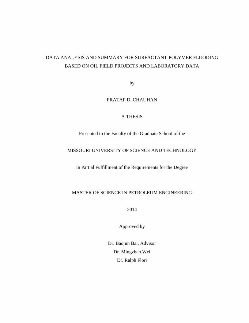
Figure 3.14 below shows a histogram of reservoir depth for 41 surfactant-polymer

chemical flooding projects. The figure shows that the peak for reservoir depth is between

1000-2000 feet. The majority of the values fall between the reservoir’s depths of 500-

1211

7

43

23

0

2

4

6

8

10

12

14

65-80 80-100 100-120 120-140 140-160 160-180 180-200

No. of

Pro

ject

s

TEMP. °F

50

2000 ft, with more than 50% of the values falling in this range. Only 1 project lies

between the highest value range of 7000 and 7500 ft.

Figure 3.14 Reservoir depth range of the dataset

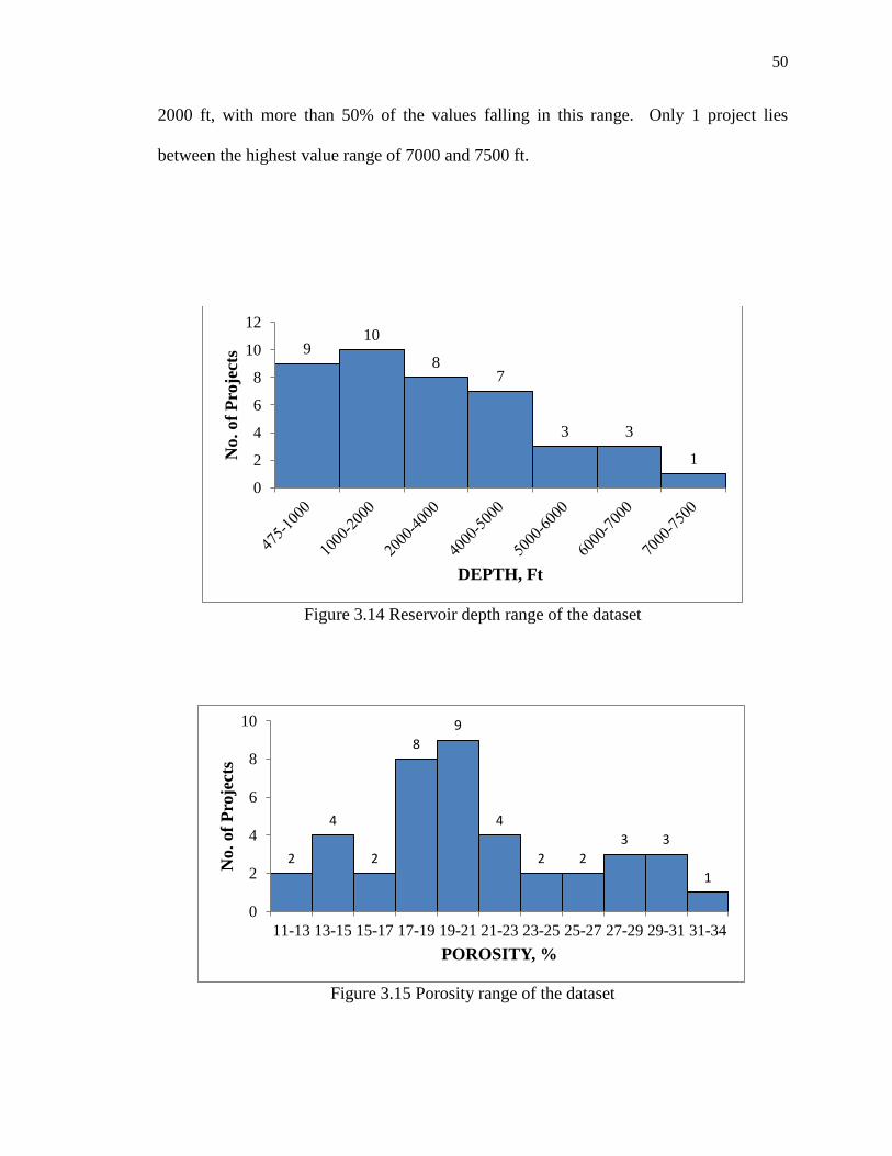
Figure 3.15 Porosity range of the dataset

910

87

3 3

1

0

2

4

6

8

10

12

No. of

Pro

ject

s

DEPTH, Ft

2

4

2

8

9

4

2 2

3 3

1

0

2

4

6

8

10

11-13 13-15 15-17 17-19 19-21 21-23 23-25 25-27 27-29 29-31 31-34

No. of

Pro

ject

s

POROSITY, %

51

Figure 3.15 shows a histogram of reservoir porosity of the dataset for 40 field

projects. The highest frequency porosity lies between 17 to 23%. Approximately 52% of

the porosity values lie in this range. The maximum porosity value of 34% is shown

between 31-34%.

Figure 3.16 Reservoir permeability range of the dataset

Figure 3.16 shows a histogram of reservoir permeability of sandstone formations.

The permeability range is across 35 field projects. 7 permeability values of reading above

1000md were excluded as special cases. These fields had high values as they consisted of

unconsolidated formation. Majority of the permeability values lie in the range of 6-

150md. Approximately 71% of the permeability values lie between 10-150md. The

minimum value of 6md was of the reservoir in Bothamsall field of the United Kingdom.

7

9

7

3

1 1

32

0

2

4

6

8

10

No. of

Pro

ject

s

PERMEABILITY, md

52

Figure 3.17 Oil viscosity range of the dataset

Figure 3.17 shows a histogram of oil viscosity of the dataset across 42 field

projects. The figure is shows high frequency to the left. The highest peak is for the range

of 3-6 cP. Approximately, 72% of the viscosity values are in the 0-12 cP range. Few oil

viscosity values ranged from 21-50 cP, with the maximum value of 50 cP. The values of

45 and 50 cP were observed for the field projects conducted in China.

Figure 3.18 shows a histogram of oil gravity °API of the dataset across 39 field

projects. It can be inferred from the histogram that most of the values lie in the range of

28-42°API suggesting that Surfactant-Polymer flooding projects are generally applied in

reservoirs containing light oil. The distribution, as can be seen is skewed to the left.

Approximately, 72% of the oil gravity values lie between the 28-41° API range.

10

14

5

3

12

12 2 2

0

2

4

6

8

10

12

14

16

0-3 3-6 6-9 9-12 12-15 15-18 18-21 21-30 30-40 40-50

No. of

Pro

ject

s

VISCOSITY, cP

53

Figure 3.18 Oil gravity range of the dataset

Figure 3.19 shows the histogram for oil saturation (start). The dataset for oil

saturation (start) comprise of 35 field projects. The highest peak in the distribution lies

between 30% and 35%. The diagram is skewed to the right. Also, 66% of the data values

fall between 30 and 40%. This is usually the residual oil saturation at the end of water-

flooding.

Figure 3.19 Oil saturation (start) range of the dataset

12

3

6

8

6

8

5

0

2

4

6

8

10

17-20 20-24 24-28 28-32 32-36 36-38 38-42 42-46

No. of

Pro

ject

s

API°

1

13

9

54

2

0

2

4

6

8

10

12

14

25.4 30-35 35-40 40-45 45-50 50-60

No. of

Pro

ject

s

OIL SAT. START, %

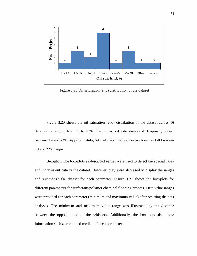
54

Figure 3.20 Oil saturation (end) distribution of the dataset

Figure 3.20 shows the oil saturation (end) distribution of the dataset across 16

data points ranging from 10 to 28%. The highest oil saturation (end) frequency occurs

between 19 and 22%. Approximately, 69% of the oil saturation (end) values fall between

13 and 22% range.

Box-plot: The box-plots as described earlier were used to detect the special cases

and inconsistent data in the dataset. However, they were also used to display the ranges

and summarize the dataset for each parameter. Figure 3.21 shows the box-plots for

different parameters for surfactant-polymer chemical flooding process. Data value ranges

were provided for each parameter (minimum and maximum value) after omitting the data

analyses. The minimum and maximum value range was illustrated by the distance

between the opposite end of the whiskers. Additionally, the box-plots also show

information such as mean and median of each parameter.

1

3

2

6

1

3

1 1

0

1

2

3

4

5

6

7

10-13 13-16 16-19 19-22 22-25 25-28 30-40 40-50

No. of

Pro

ject

s

Oil Sat. End, %

55

Figure 3.21 Left- Right-Box plots of Reservoir temperature, Depth, Oil viscosity, Oil

gravity, Reservoir porosity & permeability, Brine Salinity & Hardness, Oil saturation

start & end

0

50

100

150

200

250

TEMP, °F

0

1000

2000

3000

4000

5000

6000

7000

8000

DEPTH,

Ft

0.1

1

10

100

VISCOSITY, cP

0

10

20

30

40

50

API°

0

5

10

15

20

25

30

35

40

POROSITY, %

0

100

200

300

400

500

600

PERM., md

0

50000

100000

150000

200000

SALINITY,

ppm

1

10

100

1000

10000

HARDNESS,

ppm

0

10

20

30

40

50

60

70

OIL SAT.

START, %

0

10

20

30

40

50

60

OIL SAT.

END, %

56

Figure 3.21 shows box-plots of all the important parameters of the field projects.

The box-plots show the mean and median values of all the parameters along with the

minimum and maximum values denoted by the whiskers.

3.2 LABORATORY DATA

Most of the screening criteria work which has been published so far consists of

field projects and pilot projects for various EOR processes. However, continuous

laboratory research is been carried out to improve EOR processes. A good amount of

research is also carried out in Surfactant-polymer chemical flooding process.

A dataset of laboratory work was established comprising of experiments for

Surfactant-polymer flooding method. The dataset source comprised of information

obtained from various publications in the SPE literature of onepetro. The dataset includes

different experiments published to study properties and efficiency of surfactant-polymer

flooding. All the injection experiments were carried out in various cores to study the

efficiency of the flood for oil recovery.

Figure 3.22 Laboratory surfactant-polymer flooding experiments from 1970-2013

46, 23%

53, 26%41, 21%

60, 30%

Year 1970-1980

Year 1980-1990

Year 1990-2000

Year 2000-2013

57

Figure 3.22 shows the distribution of laboratory work on surfactant-polymer

flooding carried out over the years. It shows the number of experiments which were

conducted from 1970-2013. The turn of 20th century saw the most number of experiments

carried out to check the efficiency of SP flooding. Sixty experiments in our dataset were

executed in the years 2000 to 2013. Also, 99 experiments took place from 1970 to 1990,

which is EOR boom period.

Figure 3.23 shows the different surfactants which were used in the experiments to

establish a surfactant slug. Including the 4 basic surfactants such as Anionic, Non-ionic,

Cationic, and Zwitterionic surfactants, there emerged a class of Bio-surfactants, which

are generated through microbes and bacteria. The pie-chart (figure 3.22), illustrates the

percentage and number of experiments conducted in each category. Zwitterionic dataset

was the smallest as this class of surfactants was only recently proposed for research.

Figure 3.23 Distribution of types of Surfactants used in laboratory dataset

159, 79%

9, 5%

14, 7%

4, 2%

14, 7%

Anionic

Cationic

Non-ionic

Zwitterionic

Bio-surfactant

58

Conventional, anionic surfactants were used in most of the experiments, resulting

in the biggest dataset. Over 79% of 200 experiments used anionic surfactants to study

their effect on oil recovery.

Figure 3.24 depicts the type of polymers used in the dataset. It shows the

percentage and number of 4 different types of polymer viz. Hydrolyzed polyacrylamide,

xanthan gum, bio-polymer and associating polymer used in the experiments. HPAM was

the most common polymer used; while only a few experiments were conducted using a

new emerging class of Associating polymer.

Figure 3.24 Types of Cores used in the Laboratory dataset

Sandstone cores, sandpacks and carbonate cores were the 3 major types of cores

used in the tests. More than 80% of the tests were conducted in the sandstone cores

including Berea, Bentheimer, Briarhill and Reservoir cores. Few tests (14%) were

169, 84%

27, 14% 4, 2%

Sandstone

Sandpack

Carbonate

59

conducted in sandpacks, while even fewer were conducted in non-fractured carbonate

cores.

3.2.1. Data Analysis. Data analysis included representing the data with the help

of box-plots, histograms and cross plots.

Cross plots were used to analyze the related parameters for example, core porosity

vs. core permeability, the Oil viscosity vs. Oil gravity, Oil recovery (% of residual oil

saturation after water-flooding) vs. Surfactant slug concentration and oil viscosity.

In descriptive statistics, a box-plot is a statistical way to graphically describe a

group of numerical data by their quartiles. The box-plot used in this study divides the set

of data into 6 parts as follows.

1. The lowest value (minimum)

2. The highest value (maximum)

3. The mean value (Average data value)

4. The first quartile (25th percentile)

5. The second quartile (50th percentile)

6. The third quartile (75th percentile)

Figure 3.25 shows a schematic of a box-plot used to display the data. Histograms,

as previously used to depict the range of different reservoir and oil parameters for field

projects, were also used to observe the range of different laboratory parameters.

60

Figure 3.25 Schematic of a box-plot

Figure 3.26 shows a cross-plot of oil viscosity vs. oil gravity of the crude oil used

in different tests. One test, as is evident by the diagram showed oil viscosity of 376 cP

and gravity of 16.5°F. A test using such heavy oil was conducted to study the efficiency

of the surfactant-polymer flooding process in heavy oil reservoirs of Canada.

Figure 3.26 Cross plot of Oil viscosity vs. oil gravity

0

50

100

150

200

250

300

350

400

0 10 20 30 40 50

Oil

Vis

cosi

ty, cP

Oil Gravity, API°

61

It shows a very few data-points as some experiments used crude oil with same oil

viscosity and oil gravity. Also, many experiments only mentioned the oil viscosity and

not the oil gravity °API.

Figure 3.27 Oil viscosity histogram (left) and oil viscosity box-plot (right)

Figure 3.27 depicts the histogram and box-plot of oil viscosity values used in the

experiments. The lowest oil viscosity value was of 0.5cP while the highest oil viscosity

value was of 550cP, which is denoted by the >32 bar in the histogram. It can be inferred

from such high oil viscosities that the surfactant-polymer flooding is being tested for

recovery efficiency of heavy crude oil, to increase the application range of the method.

3

34

57

13

5 5

0

10

20

30

40

50

60

0.5 1.25-4 4-8 8-16 16-32 >32

No. of

Exp

erim

ents

OIl VISCOSITY, cP

0.1

1

10

100

1000

VISCOSITY,

cP

62

Figure 3.28 Oil Gravity histogram (left) and oil gravity box-plot (right)

Figure 3.28 shows the range of oil gravity °API with the help of histogram and

the box-plot. The minimum value was 14.5° API and further the low values observed

were between the values of 14.5 to 20°API. Such low values were observed for the

experiments in which heavy crude oil with high viscosity were used. The new proposed

class of zwitterionic (amphoteric) surfactants was tested for recovery in heavy oil

reservoirs. A few experiments were conducted for a crude oil with viscosity of 75cP. An

Alkoxy Carboxylate surfactant with large hydrophobic tail was used to check its stability

in the presence of high viscosity oil. Oil recovery results for these experiments showed

promising results.

4 3 4 4

39

20

8

0

5

10

15

20

25

30

35

40

45

No. of

Exp

erim

ents

OIL GRAVITY, API°

0

5

10

15

20

25

30

35

40

45

50

Oil Gravity,

API°

63

Figure 3.29 Cross-plot of core permeability vs. core porosity

Figure 3.29 shows a cross-plot of core permeability vs. core porosity. The data-

points show a consistent relationship between the porosity and permeability values.

However, five peremeability values lie on the higher side, over 1000md. These high

permeability values were observed for sandpacks. Sandpacks are the loosely packed

grains of sand which are generally used to observe the behaviour of the chemical slug in

the formation and its interaction when it comes in contact with the crude oil. The

minimum value observed in the cross-plot was of 106 md of reservoir core.

0

5

10

15

20

25

30

35

40

45

0 1000 2000 3000 4000 5000 6000

Poro

sity

, %

Permeability, md

64

Figure 3.30 Core porosity histogram (above) and core porosity box-plot (below)

Figure 3.30 represents the range of core porosity with the help of a histogram and

a boxplot. As we study the diagram, it can be inferred that the highest peak of core

porosities was observed in the range of 18 to 22. Approximately, 76 percent of the

porosity values lie between 14-26%. The lowest value of porosity observed was of

1

5

1

22

41

27

2

911

0

5

10

15

20

25

30

35

40

45

No. of

Exp

erim

ents

POROSITY, %

0

5

10

15

20

25

30

35

40

45

POROSITY, %

65

6.47%. This value was the porosity value measured for a reservoir core. The porosity

box-plot shows a spread of porosity values between 6.47 to 41%, with the mean at

23.9%.

Figure 3.31 permeability histogram (above) and permeability box-plot (below)

1 0

8

15

31

48

30

911

1 1 2

0

10

20

30

40

50

60

No. of

Exp

erim

ents

PERMEABILITY, md

0

1000

2000

3000

4000

5000

6000

PERMEABILITY,

md

66

Figure 3.31 shows the distribution of permeability values for the different cores

used in the tests. It can be concluded from the histogram and permeability box-plot that

the permeability values are spread over a wide range from 9.8md to over 5000md.

Majority of the values in the dataset lie between 70 and 800. However, the permeability

values vary significantly from one core to other core, for instance, one of the reservoir

core permeability was 2668md, while most of the reservoir cores had permeability values

of less than 1000md. Also, the high permeability values (greater than 1000md) are

observed for sandpacks and few Bentheimer cores.

Figure 3.32 Surfactant slug concentration histogram (left) and box-plot (right)

Figure 3.32 gives the range for surfactant slug concentration used in the tests in

2

12 13

24

32

28

17

30

8

35

1

0

5

10

15

20

25

30

35

No. of

Exp

erim

ents

SURFACTANT CONC., ppm

1

10

100

1000

10000

100000

SURFACTANT

CONC., ppm

67

our dataset. Majority of the values lie in the range of 5000 to 40,000 parts per million

(ppm). Approximately 77% of the 175 surfactant concentration values lie in the

aforementioned range. It can also be inferred that a few values are as low as 2.8ppm.

Concentrations of bio-surfactants used in a few experiments had a range of 2.8ppm to

41ppm. The box-plot of surfactant slug concentration shows a mean of 20,355.6ppm.

High concentration of surfactant slug (over 50,000ppm) in the subset was observed for

tests which used surfactant blend of petroleum sulfonate and non-ionic surfactant. The

concentration measured was a combination of these surfactants.

Figure 3.33 Surfactant slug size histogram (left) and box-plot (right)

1

19

33

61

24

41

0

10

20

30

40

50

60

70

0.03 0.03-0.1 0.1-0.3 0.3-0.5 0.5-1 1-2 2-3

No. of

Exp

erim

ents

SURFACTANT SLUG SIZE, PV0

0.5

1

1.5

2

2.5

3

3.5

SURFACTANT PV

68

Figure 3.33 depicts the range of surfactant slug size in terms of pore volume

injected. The surfactant slug size of the subset ranged from 0.03 to 3. As can be inferred

from the plots, majority of the values lie between 0.041 and 0.9. The surfactant slug size

over 1PV were used in bio-surfactant tests.

Figure 3.34 Polymer drive concentration histogram (left) and box-plot right

Figure 3.34 illustrates the range of polymer drive concentration (parts per million)

with the help of a histogram and box plot. Majority of the tests were conducted with

polymer concentration of 800 to 2000 ppm. 74 of the 121 values in the subset lie in this

2 4 2

64

30

85 4 3

0

10

20

30

40

50

60

70

No. of

Exp

erim

ents

POLYMER DRIVE CONC., ppm

0

1000

2000

3000

4000

5000

6000

POLYMER

CONC., ppm

69

range. Few values in the dataset were high in the range of 4000-5000ppm. These were

bio-polymer concentrations.

Figure 3.35 Polymer drive slug size histogram (left) and box-plot (right)

Figure 3.35 gives the range of polymer drive slug size in terms of total pore

volume injected. The minimum value observed in the dataset was 0.35 PV while the

maximum value observed was 2.8 PV. Majority of the values in this subset were in the

range of 0.5PV to 1.5 PV. The maximum slug size of 2.8 PV was observed for a test

conducted in reservoir sandstone core to achieve a favourable mobility ratio.

14

20

46

13

0

5

10

15

20

25

30

35

40

45

50

0.35 0.35-0.5 0.5-0.9 1-1.5 1.5-1.7 >3

No. of

Exp

erim

ents

POLYMER DRIVE, PV

0

0.5

1

1.5

2

2.5

3

POLYMER,

PV

70

Figure 3.36 IFT between oil-water-surfactant system histogram (left) and box-plot (right)

Figure 3.36 shows the interfacial tension (IFT) values between oil-surfactant-

water system. It can be inferred that the IFT values in the dataset had a wide spread from

0.0001 dynes/cm to 4.2 dynes/cm. The higher IFT values were observed for the oil-

surfactant-water system in which bio-surfactants were used. Also, as can be interpreted

from the IFT box-plot, the mean of the subset 0.274 dynes/cm because of these high

values ranging from 1 dynes/cm to 4.2 dynes/cm.

Figure 3.37 shows the range of dynamic adsorption of anioinic surfactants on

sandstone adsorbent. The adsorption was measured in terms of milligrams of surfactant

adsorbed per gram of adsorbent. Majority of the adsorption values ranged from 0.1mg/g

to 0.6mg/g. Few of the surfactants had high surfactant adsorption, ranging from 1 mg/g to

4.2 mg/g. These were observed for reservoir sandstone cores, where adsorption increases

due to reservoir heterogenity.

1

32

38

12

4 5 53 2 2 2 2

0

5

10

15

20

25

30

35

40

No. of

Exp

erim

ents

IFT, dynes/cm

0.00001

0.0001

0.001

0.01

0.1

1

10

IFT,

dynes/cm

71

Figure 3.37 Dynamic adsorption histogram (left) and box-plot (right)

Figure 3.38 Static adsorption box-plot

1

4

13

11

13 13

21

0

21

21

0

2

4

6

8

10

12

14

No. of

Exp

erim

ents

DYNAMIC ADSORPTION, (mg/g)

0.01

0.1

1

10

DYNAMIC

ADSORPTION,mg/g

0

10

20

30

40

50

60

70

Static Adsorption, mg/g

72

Figure 3.38 shows the range of static adsorption of anionic surfactants on

kaolinite adsorbent. It can be inferred from the box-plot that the adsorption ranges from

0.4 mg/g to as high as 66.1 mg/g. When compared with dynamic adsorption, static

adsorption has higher values. This can be attributed to kaolinite adsorbent used in the

static adsorption experiments. Since clay has higher surface area than sandstone, more

surfactant is adsorbed on it.

Figure 3.39 Brine salinity histogram (right) and box-plot (left)

Figure 3.39 shows the brine salinity distribution with the help of a histogram and

a box-plot. It can be inferred from the graph that the minimum and maximum values for

2 1

22

13

17

13

33

8 8

17

1

12

4

0

5

10

15

20

25

30

35

No. of

Exp

erim

ents

BRINE SALINITY, ppm

0

50000

100000

150000

200000

250000

BRINE

SALINITY,

ppm

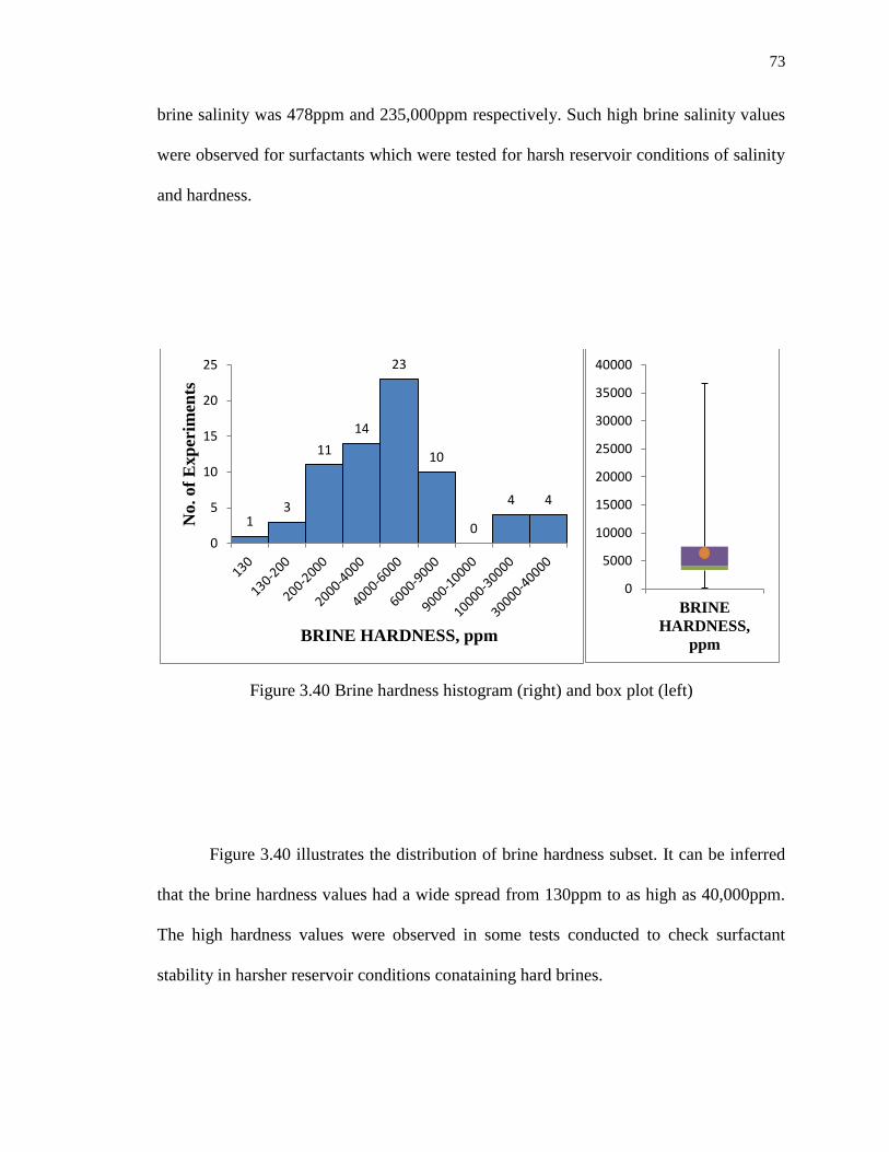
73

brine salinity was 478ppm and 235,000ppm respectively. Such high brine salinity values

were observed for surfactants which were tested for harsh reservoir conditions of salinity

and hardness.

Figure 3.40 Brine hardness histogram (right) and box plot (left)

Figure 3.40 illustrates the distribution of brine hardness subset. It can be inferred

that the brine hardness values had a wide spread from 130ppm to as high as 40,000ppm.

The high hardness values were observed in some tests conducted to check surfactant

stability in harsher reservoir conditions conataining hard brines.

13

11

14

23

10

0

4 4

0

5

10

15

20

25

No. of

Exp

erim

ents

BRINE HARDNESS, ppm

0

5000

10000

15000

20000

25000

30000

35000

40000

BRINE

HARDNESS,

ppm

74

Figure 3.41 Temperature histogram (left) and box plot (right)

Figure 3.41 shows the range of temperatures under which the experiments were

conducted. The values show a wide range of spread between 20°C to 177°C. It can be

inferred from the figure that few experiments were conducted under high temperatures

for instance; one test was conducted at a temperature of 177°C (350°F) to test the

stability of surfactant (akyl aryl sulfonate) at such high temperature.

Figure 3.42 illustrates a cross plot of Surfactant slug concentration (parts per

million) vs. the tertiary oil recovery of fraction of oil in place after waterflooding for all

the tests performed. The oil recovery, as can be concluded varies significantly from core

to core. This prominent difference between oil recoveries for the cores can be attributed

to the type of cores being used to check the efficiency of the surfactant-polymer flooding.

Berea sandstone cores, Briarhill sandstone cores, Bentheimer sandstone cores were used

in most of the tests. These standard cores are more homogenous than the reservoir cores.

3

51

29

42

15 14

72

9

2 10

10

20

30

40

50

60

No. of

Exp

erim

ents

TEMPERATURE, °C

0

20

40

60

80

100

120

140

160

180

200

TEMPERATURE, °C

75

Figure 3.42 Cross-plot of surfactant concentration vs. tertiary oil recovery (after

waterflooding)

Low residual oil recovery in the reservoir cores was attributed to the

heterogeneity of the rock, which affected the stability of the chemical slug which resulted

in higher surfactant retention (adsorption) and affected the micro-emulsion phase, which

in turn affected the size of the oil bank formed. Surfactant slug concentration injected in

the cores also affected the tertiary oil recovery. For example, in tests where low

concentration of bio-surfactants was used, the oil recovery was poor. However, when

high concentration of surfactants (47,600 ppm) was injected in a core, all of the residual

oil was recovered as indicated by the cross-plot above. Figure 3.43 shows the range of

percentage of tertiary oil recovery after waterflooding. The values of the subset had a

wide spread between 19.5% to 100% tertiary oil recovery. Most of the low oil recoveries

0

20

40

60

80

100

120

0 10000 20000 30000 40000 50000 60000 70000 80000 90000

Ter

tiary

oil

rec

over

y,

%

Surfactant Concentration, ppm

76

were observed for reservoir sandstone cores, while higher tertiary oil recoveries were

measured for more homogenous Berea sandstones, Briarhill sandstones.

Figure 3.43 Tertiary oil recovery histogram (right) and box-plot (left)

Figure 3.44 Residual oil saturation box-plot

1

8 7

14

1923

38

33

24

0

5

10

15

20

25

30

35

40

No. of

Exp

erim

ents

TERTIARY OIL RECOVERY, %Sor

0

10

20

30

40

50

60

70

80

90

100

TERTIARY OIL

RECOVERY, %

0

10

20

30

40

50

60

RESIDUAL OIL

SATURATION,

%

77

4. SUMMARY AND CONCLUSION

After, detailed representation of both field and laboratory datasets, the established

summary was presented in the following section. Summary for field projects was

compared to the previous work. Eventually, a comparison was made between the

established ranges of laboratory and field datasets.

4.1 SUMMARIZING THE FIELD DATASET

Table 4.2 below gives the range for surfactant-polymer flooding on the basis of

statistical analysis for a cleaned dataset. The summary includes all the parameters which

eventually decide success or failure of a surfactant-polymer flooding project. The

statistical parameters used to define the range were mean, median, standard deviation,

minimum and maximum values.

The ranges for the parameters was eventually compared with the previous work

and the differences were noted.

1. The concluded summary of oil gravity had a range from 17°API to 45°API.

Brasear (1978), Carcaoana (1982) and Goodlett (1986) suggested a value

greater than 25°API, while Taber (1997) suggested a value to be greater than

20°API. Aldasani and Bai gave a range of 22°API to 39°API, with and

average value of 34.8°API.

78

2. Oil viscosity in the study has a range of 0.32cP to 50cP, while authors like

Caracoana (1982), Peter H. (2984) and Goodlett (1986) suggested a value less

than 30cP. On the other hand, Taber (1997) suggested a value of less than

35cP for oil viscosity. Aldasani and Bai concluded a range of 15.6 to 3 cP and

a mean of 9.3cP.

3. Temperature range in the study was from 65°F to 200°F. Most of the authors

suggested the value to be less than 200°F (Table 2.3), while Caracoana (1982)

and Al-Bahar (2004) suggested a value less than 180°F and 158°F

respectively. The temperature range differed from previous work conducted

by Aldasani and Bai, as they concluded a range of 122-155°F with a mean of

138.5°F

4. Depth range was concluded to be between 475 ft to 7500ft which differed

from the values of less than 7000ft and 9000ft suggested by Caracoana (1982)

and Goodlett (1986) respectively.

5. Porosity value ranged from 11 to 34% in the study. However, Brashear

(1978), Caracoana (1982) and Goodlett (1986) suggested a value of greater

than 20%.

6. Permeability range was concluded to be between 6md and 500md. This range

differed from the value proposed by most of the authors. Brashear (1978),

Caracoana (1982), Peter H. (1984), Goodlett (1986), Taber (1997) and Al-

Bahar (2004) suggested a value greater than 20md, 35md, 40md, 40md, 40md

and 50md respectively.

79

Table 4.1 Summary of ranges for surfactant-polymer flooding for field dataset

Parameters

Mean Median

Standard

Deviation Minimum Maximum

Oil Gravity, °API 34.8 35 6.9 17 45

Oil Viscosity, cP 10.8 5 12.7 0.32 50

Temperature, °F 109.4 100 38.7 65 200

Depth, ft

3088 2200 2062 475 7500

Porosity, %

21.5 20 5.6 11 34

Permeability, md 150.9 103 135.64 6 500

Oil saturation start, % 39 40 8 25.4 58

Oil saturation end, % 22.7 20 9.6 10 50

Brine salinity, ppm 40,508 16,500 43,833 400 160,000

Brine hardness, ppm 1559 70 2166 13 6530

7. The minimum oil saturation start value in the dataset was 25.4%. This differed

from the values suggested by Brashear (1978), Caracoana (1982), Goodlett

(1986), Al-Bahar (2004), which were 25%, 30%, 30% and 35% respectively.

Taber (1997) suggested a value of greater than 35%. Aldasani and Bai gave a

higher range of 43.5 to 53.

80

8. The maximum salinity value in the dataset was 160,000ppm which differed

from the maximum salinity values of 50,000ppm, 100,000, 140,000 and

50,000 proposed by Brashear, Peter H., Goodlett and Al-Bahar respectively.

The study on laboratory dataset showed a distinct difference than the field project

dataset for surfactant-polymer flooding. The statistical data for different parameters have

different ranges for laboratory dataset. Table 4.2 shows parameters like oil viscosity, oil

gravity, temperature, porosity, permmeability, oil saturation start (residual oil saturation),

tertiary oil recovery by surfactant-ploymer flooding, surfactant concentration, brine

salinity, IFT and adsorption. IFT, surfactant adsorption and surfactant concentration were

3 parameters studied for laboratory dataset. A comparison between the field project

dataset and laboratory dataset follows.

1. The obvious difference between maximum oil viscosities of field maximum

(50cP) and laboratory criteria (550cP) was due to the use of new emerging

visco-elastic surfactants used for recovery of heavy oil. Laboratory dataset

contained an experiment which was tested for recovery of oil of viscosity

376cP. A new class of surfactants called Zwitterionic (amphoteric) surfactant

was used in this experiment. Both the experiments were successful in terms of

tertiary oil recovery.

81

Table 4.2 Summary of ranges for surfactant-polymer flooding for Lab. dataset

Parameters

Mean Median

Standard

Deviation Minimum Maximum

Oil Gravity, °API 30.5 30.6 6.6 14.5 44

Oil Viscosity, cP 16.3 5.2 61.4 0.5 550

Temperature, °C 46 42 23.3 20 177

Porosity, %

22.9 20 7.8 6.47 41

Permeability, md 657 529.5 845 9.8 5415

Oil Saturation (Start) 35.8 36 5.9 15.1 55

Oil Saturation (end) 12.5 11.45 8.3 0.5 38

Surfactant

Concentration, ppm 20355.6 16000 17755 2.8 80000

Surfactant

slug Size, PV

0.48 0.45 0.42 0.03 3

IFT, dynes/cm 0.274 0.005 0.79 0.0001 4.2

Adsorption, mg/g-

Dynamic 0.55 0.34 0.78 0.027 4.51

Static

25.57 20.7 19.38 0.4 66.1

Brine Salinity, ppm 81154 50000 83294 478 350000

Brine Hardness, ppm 6398 4050 7989 130 36633

Polymer Drive size,

PV 1.05 1 0.46 0.35 2.8

2. Maximum temperature value for field range was 185°F (85°C), which was

Polymer Drive

Conc. ppm

1718 1500 1057 350 5500

Tertiary Oil

Recovery, (%Sor) 69.7 75 19.59 19.5 100

82

far less than the value of 177°C (351°F) observed in laboratory range.

Experiment for high temperature resistant surfactant for steam assisted

surfactant-polymer flooding was conducted and was fairly successful in

recovering the residual oil after waterflooding.

3. Permeability and porosity maximum values differed from 30% and 500md

(0.5 D) to 48% and 5.5 D (5415md) for field and laboratory criteria

respectively. This difference was due to the highly permeable sandpacks used

in laboratory experiments. A new method of gravity stable surfactant flooding

for horizontal wells with high vertical permeability was tested sucessfully

using sandpacks.

4. Maximum residual oil saturation value varied from 58% for field range to

55% for laboratory range. This difference was noted as heavy oil resulted in

poor waterflooding recovery and a class of new surfactants was tested for

tertiary oil recovery of such heavy oil reservoirs in Canada.

5. Brine salinity and brine hardness maximum values for field were 160,000 and

6,530 ppm. However, for laboratory the values were 350,000 ppm and 36,633.

Such high maximum salinity and hardness values were due to the laboratory

research carried out to test the stability of surfactants and yield a low IFT

value at the same time in highly saline and hard brines.

4.2 CONCLUSION

1. This work gives a detailed description of steps followed to give an updated range

for surfactant-polymer flooding on a field and laboratory scale.

83

2. The field dataset was checked for special cases and inconsistent values for various

parameters with the help of histograms and box-plots.

3. Ranges for different imperative laboratory parameters were presented graphically

using histograms and box-plots.

4. Eventually, field ranges were compared with the previous work published in the

literature and sought for differences.

5. Laboratory and field ranges were compared and their differences were explained.

84

BIBLIOGRAPHY

1. Enhanced Oil Recovery- Don W. Green & Paul Willhite (1998)

2. E. Manrique et.al., Norwegian University of Science and technology- Chemical

flooding projects for enhanced oil recovery (2010)

3. Istvan Lakatos et. al., University of Miskolc, Role of conventional and

Unconventional hydrocarbons in the 21st century: comparison of resources,

reserves, recovery factors and Technologies. (2009)

4. Department of Energy (DOE), Chemical flooding projects for unconventional

hydrocarbons (1993)

5. Schramm L. L., Surfactants fundamental and application in petroleum industry,

(2000)

6. Levitt D.B., Identification and evaluation of high-performance EOR surfactant

(University of Texas- Austin, 2006)

7. Gary Walker (DOE), Increasing heavy oil reserves in the Willmington oilfield

through advanced reservoir characterization and thermal production technologies.

(Annual report, March 31, 2000)

8. Alhasan Fuseni (Saudi Aramco), Phase behavior and interfacial tension properties

of an amphoteric surfactant for EOR application. (2013)

9. Jean-Louis Salager, Surfactant types and uses. (2002)

10. Xianmin Zhou et. al. Adsorption of an amphoteric surfactant onto permeable

carbonate rocks. (2013)

11. Bataweel, M. A., Yadhalli Shivaprasad, A., & Nasr-El-Din, H. A. (2012, January

1). Low-Tension Polymer Flooding Using Amphoteric surfactant in High

Salinity/High Hardness and High Temperature Conditions in Sandstone Cores.

Society of Petroleum Engineers. doi:10.2118/155676-MS

85

12. Gao, B., & Sharma, M. M. (2013, June 6). A New Family of Anionic Surfactants

for Enhanced-Oil-Recovery Applications. Society of Petroleum Engineers.

doi:10.2118/159700-PA

13. Healy, R. N., & Reed, R. L. (1974, October 1). Physsicochemical Aspects of

Microemulsion Flooding. Society of Petroleum Engineers. doi:10.2118/4583-PA

14. Wade, W. H., Morgan, J. C., Schechter, R. S., Jacobson, J. K., & Salager, J. L.

(1978, August 1). Interfacial Tension and Phase Behavior of Surfactant Systems.

Society of Petroleum Engineers. doi:10.2118/6844-PA

15. J Salager, J. L., Morgan. C., Schechter, R. S., Wade, W. H., & Vasquez, E. (1979,

April 1). Optimum Formulation of Surfactant/Water/Oil Systems for Minimum

Interfacial Tension or Phase Behavior. Society of Petroleum Engineers.

doi:10.2118/7054-PA

16. Winsor P. A. Binary and Muticomponent solution of amphiphilic compunds.

Solubalization and the formation, structure and theoretical significance of liquid

crystalline solutions (1967).

17. Thomas, S. (2006, January 1). Chemical EOR: The Past - Does It Have a Future?

(Russian). Society of Petroleum Engineers.

18. Salter, S. J. (1977, January 1). The Influence Of Type And Amount Of Alcohol

On Surfactant-Oil-Brine Phase Behavior And Properties. Society of Petroleum

Engineers. doi:10.2118/6843-MS

19. Li, R. F., Le Bleu, R. B., Liu, S., Hirasaki, G. J., & Miller, C. A. (2008, January

1). Foam Mobility Control for Surfactant EOR. Society of Petroleum Engineers.

doi:10.2118/113910-MS

20. Trogus, F. J., Sophany, T., Schechter, R. S., & Wade, W. H. (1977, October 1).

Static and Dynamic Adsorption of Anionic and Nonionic Surfactants. Society of

Petroleum Engineers. doi:10.2118/6004-PA

21. Schamehorn, J. F., Schechter, R. S., Wade W.H. (1981, April 22). Adsorption of

Surfactants on Mineral oxide Surfaces from Aqueous Solutions.

86

22. Ziegler, V. M., & Handy, L. L. (1981, April 1). Effect of Temperature on

Surfactant Adsorption in Porous Media. Society of Petroleum Engineers.

doi:10.2118/8264-PA

23. Dang, C. T. Q., Chen, Z. J., Nguyen, N. T. B., Bae, W., & Phung, T. H. (2011,

January 1). Development of Isotherm Polymer/Surfactant Adsorption Models in

Chemical Flooding. Society of Petroleum Engineers. doi:10.2118/147872-MS

24. Davis, H. T., & Scriven, L. E. (1980, January 1). The Origins Of Low Interfacial

Tensions For Enhanced Oil Recovery. Society of Petroleum Engineers.

doi:10.2118/9278-MS

25. Cinar, Y., & Orr, F. M. (2004, January 1). Measurement of Three-Phase Relative

Permeability with IFT Variation. Society of Petroleum Engineers.

doi:10.2118/89419-MS

26. Delshad, M., Delshad, M., Bhuyan, D., Pope, G. A., & Lake, L. W. (1986,

January 1). Effect of Capillary Number on the Residual Saturation of a Three-

Phase Micellar Solution. Society of Petroleum Engineers. doi:10.2118/14911-MS

27. Bashiri, A., & Kasiri, N. (2011, January 1). Properly Use Effect of Capillary

Number on Residual Oil Saturation. Society of Petroleum Engineers.

doi:10.2118/150800-MS

28. Sheng, J. J. (2013, April 19). A Comprehensive Review of Alkaline-Surfactant-

Polymer (ASP) Flooding. Society of Petroleum Engineers. doi:10.2118/165358-

MS

29. Wei, H. (2012, January 1). Molecular Design Synthesis and Simulation on a

Novel Gemini Surfactant for EOR From Low Permeability Reservoirs. Society of

Petroleum Engineers. doi:10.2118/160854-MS

30. Gogarty, W. B. (1978, August 1). Micellar/Polymer Flooding An Overview.

Society of Petroleum Engineers. doi:10.2118/7041-PA

31. Hite, J. R., & Bondor, P. L. (2004, January 1). Planning EOR Projects. Society of

Petroleum Engineers. doi:10.2118/92006-MS

87

32. Manrique, E. J., Thomas, C. P., Ravikiran, R., Izadi Kamouei, M., Lantz, M.,

Romero, J. L., & Alvarado, V. (2010, January 1). EOR: Current Status and

Opportunities. Society of Petroleum Engineers. doi:10.2118/130113-MS

33. Thomas, S., & Ali, S. M. F. (1992, August 1). Micellar-Polymer Flooding: Status

And Recent Advances. Petroleum Society of Canada. doi:10.2118/92-08-05

34. Hirasaki, G. J., Miller, C. A., & Puerto, M. (2008, January 1). Recent Advances in

Surfactant EOR. Society of Petroleum Engineers. doi:10.2118/115386-MS

35. Brashear, J. P., & Kuuskraa, V. A. (1978, September 1). The Potential and

Economics of Enhanced Oil Recovery. Society of Petroleum Engineers.

doi:10.2118/6350-PA

36. Carcoana, A. N. (1982, January 1). Enhanced Oil Recovery in Rumania. Society

of Petroleum Engineers. doi:10.2118/10699-MS

37. Putz, A., Chevalier, J. P., Stock, G., & Philippot, J. (1981, April 1). A Field Test

of Microemulsion Flooding, Chateaurenard Field, France. Society of Petroleum

Engineers. doi:10.2118/8198-PA

38. Aguey, O. J. (1982, January 1). Field Performance Analysis of Micellar Polymer

Pilot Flood. Society of Petroleum Engineers. doi:10.2118/10732-MS

39. Gupta, S. P. (1984, February 1). Compositional Effects on Displacement

Mechanisms of the Micellar Fluid Injected in the Sloss Field Test. Society of

Petroleum Engineers. doi:10.2118/8827-PA

40. Staub, H. L. (1981, January 1). Results Of A Micellar-Polymer Flood In A

Flooded-Out, Low Gravity Reservoir. Society of Petroleum Engineers.

doi:10.2118/9791-MS

41. Aho, G. E., & Bush, J. (1982, January 1). Results of the Bell Creek Unit

&apos;A&apos; Micellar-Polymer Pilot. Society of Petroleum Engineers.

doi:10.2118/11195-MS

42. Hamaker, D. E., & Frazier, G. D. (1978, January 1). Manvel Enhanced Recovery

Pilot Design And Implementation. Society of Petroleum Engineers.

doi:10.2118/7088-MS

88

43. Cooper, M. N., Southworth, R. A., Walsh, D. M., & Morgan, J. C. (1985, January

1). Field Experience In The Bothamsall Surfactant Flood Project. Society of

Petroleum Engineers. doi:10.2118/13990-MS

44. Luo, P., Wu, Y., & Huang, S.-S. S. (2013, June 11). Optimized Surfactant-

Polymer Flooding for Western Canadian Heavy Oils. Society of Petroleum

Engineers. doi:10.2118/165396-MS

45. Lu, J., Britton, C., Solairaj, S., Liyanage, P. J., Kim, D. H., Adkins, S., … Pope,

G. A. (2012, January 1). Novel Large-Hydrophobe Alkoxy Carboxylate

Surfactants for Enhanced Oil Recovery. Society of Petroleum Engineers.

doi:10.2118/154261-MS

46. Ziegler, V. M. (1988, May 1). Laboratory Investigation of High Temperature

Surfactant Flooding. Society of Petroleum Engineers. doi:10.2118/13071-PA

47. Morvan, M., Degre, G., Beaumont, J., Dupuis, G., Zaitoun, A., Al-maamari

Rashid Salim, … Al-Sharji, H. H. (2012, January 1). Optimization of

Viscosifying Surfactant Technology for Chemical EOR. Society of Petroleum

Engineers. doi:10.2118/154053-MS

48. Bae, J. H., & Petrick, C. B. (1986, November 1). Glenn Pool Surfactant Flood

Pilot Test: Comparison of Laboratory and Observation-Well Data. Society of

Petroleum Engineers. doi:10.2118/12694-PA

49. Murtada, H., & Marx, C. (1982, December 1). Evaluation of the Low Tension

Flood Process for High-Salinity Reservoirs-Laboratory Investigation Under

Reservoir Conditions. Society of Petroleum Engineers. doi:10.2118/8999-PA

50. Pope, G. A., Weerasooriya, U. P., & Lu, J. (2013, April 8). Stability Investigation

in Low-Tension Surfactant Floods. Society of Petroleum Engineers.

doi:10.2118/164090-MS

51. Sarma, H. K., Maini, B. B., & Jha, K. (1998, July 1). Evaluation of Emulsified

Solvent Flooding For Heavy Oil Recovery. Petroleum Society of Canada.

doi:10.2118/98-07-06

52. Stournas, S. (1983, January 1). Brine-Resistant Sulfonate Surfactants for

Enhanced Oil Recovery. Society of Petroleum Engineers. doi:10.2118/11773-MS

64.

89

53. Lu, J., Weerasooriya, U. P., Solairaj, S., Kim, D. H., Liyanage, P. J., Pope, G. A.,

… Britton, C. (2013, March 26). Recent Technology Developments in

Surfactants and Polymers for Enhanced Oil Recovery. International Petroleum

Technology Conference. doi:10.2523/16425-MS

54. Nguyen, P.-T., Do, B.-P. H., Pham, D.-K., Nguyen, Q.-T., Dao, D.-Q. P., &

Nguyen, H.-A. (2012, January 1). Evaluation on the EOR Potential Capacity of

the Synthesized Composite Silica-Core/ Polymer-Shell Nanoparticles Blended

with Surfactant Systems for the HPHT Offshore Reservoir Conditions. Society of

Petroleum Engineers. doi:10.2118/157127-MS

55. Ibrahim, Z. B., Manap, A. A. A., Hamid, P. A., Hon, V. Y., Lim, P. H., & Wyatt,

K. (2006, January 1). Laboratory Aspect of Chemical EOR Processes Evaluation

for Malaysian Oilfields. Society of Petroleum Engineers. doi:10.2118/100943-

MS

56. Bouabboune, M., Hammouch, N., & Benhadid, S. (2006, January 1). Comparison

Between Micro-Emulsion and Surfactant Solution Flooding Efficiency for

Enhanced Oil Recovery in TinFouye Oil Field. Petroleum Society of Canada.

doi:10.2118/2006-058

57. Maudgalya, S., Knapp, R. M., McInerney, M. J., Folmsbee, M., & Nagle, D. P.

(2005, January 1). Tertiary Oil Recovery With Microbial Biosurfactant

Treatment of Low-Permeability Berea Sandstone Cores. Society of Petroleum

Engineers. doi:10.2118/94213-MS

58. Michels, A. M., Djojosoeparto, R. S., Haas, H., Mattern, R. B., van der Weg, P.

B., & Schulte, W. M. (1996, August 1). Enhanced Waterflooding Design With

Dilute Surfactant Concentrations for North Sea Conditions. Society of Petroleum

Engineers. doi:10.2118/35372-PA

59. Najurieta, H. L., Galacho, N., Chimienti, M. E., & Illiano, S. N. (2001, January

1). Effects of Temperature and Interfacial Tension in Different Production

Mechanisms. Society of Petroleum Engineers. doi:10.2118/69398-MS

60. Tabary, R., Douarche, F., Bazin, B., Lemouzy, P. M., Moreau, P., & Morvan, M.

(2012, January 1). Design of a Surfactant/Polymer Process in a Hard Brine

Context: A Case Study Applied to Bramberge Reservoir. Society of Petroleum

Engineers. doi:10.2118/155106-MS

90

61. Hill, H. J., Reisberg, J., 10& Stegemeier, G. L. (1973, February 1). Aqueous

Surfactant Systems For Oil Recovery. Society of Petroleum Engineers.

doi:.2118/3798-PA

62. Wasan, D. T., Shah, S. M., Aderangi, N., Chan, M. S., & McNamara, J. J. (1978,

December 1). Observations on the Coalescence Behavior of Oil Droplets and

Emulsion Stability in Enhanced Oil Recovery. Society of Petroleum Engineers.

doi:10.2118/6846-PA

63. Al-Adasani, A., & Bai, B. (2010, January 1). Recent Developments and Updated

Screening Criteria of Enhanced Oil Recovery Techniques. Society of Petroleum

Engineers. doi:10.2118/130726-MS

91

VITA

Pratap Chauhan earned his under graduate degree (B.Sc.) in Geology from

University of Pune, Maharashtra, India in spring 2009. He earned a master’s degree in

Petroleum Technology (M.Sc) from University of Pune in the spring of 2011. In August,

2014, he received his Master in Petroleum Engineering degree from Missouri University

of Science and Technology.