Alireza Ashayer April, 2019 Director of Thesis: Dr. Nasseh ...

MODELING AND PREDICTION OF CRYPTOCURRENCY PRICES USING MACHINE

LEARNING TECHNIQUES

by

Alireza Ashayer

April, 2019

Director of Thesis: Dr. Nasseh Tabrizi

Major Department: Department of Computer Science

With the introduction of Bitcoin in the year 2008 as the first practical decentralized cryptocurrency,

the interest in cryptocurrencies and their underlying technology, Blockchain, has skyrocketed. Their

promise of security, anonymity, and lack of a central controlling authority make them ideal for users

who value their privacy. Academic research on machine learning, Blockchain technology, and their

intersection have increased significantly in recent years. Specifically, one of the interest areas for

researchers is the possibility of predicting the future prices of these cryptocurrencies using

supervised machine learning techniques. In this thesis, we investigate their ability to make one day

ahead price prediction of several popular cryptocurrencies using five widely used time-series

prediction models. These models are designed by optimizing model parameters, such as activation

functions, before settling on the final models presented in this thesis. Finally, we report the

performance of each time-series prediction model measured by its mean squared error and accuracy

in price movement direction prediction.

MODELING AND PREDICTION OF CRYPTOCURRENCY PRICES USING MACHINE

LEARNING TECHNIQUES

A Thesis

Presented to the Faculty of the Department of Computer Science

East Carolina University

In Partial Fulfillment of the Requirements for the Degree

Master of Science in Software Engineering

by

Alireza Ashayer

April, 2019

MODELING AND PREDICTION OF CRYPTOCURRENCY PRICES USING MACHINE LEARNING

TECHNIQUES

SIGNATURE PAGE

by

Alireza Ashayer

APPROVED BY:

DIRECTOR OF

THESIS: _____________________________________________________________________________________

Nasseh Tabrizi, PhD

COMMITTEE MEMBER: _______________________________________________________________________

Krishnan Gopalakrishnan, PhD

COMMITTEE MEMBER: _______________________________________________________________________

Sergiy Vilkomir, PhD

CHAIR OF THE DEPARTMENT

OF COMPUTER SCIENCE: _________________________________________________________________

Venkat N. Gudivada, PhD

DEAN OF THE

GRADUATE SCHOOL: ________________________________________________________________________

Paul J. Gemperline, PhD

This thesis is dedicated to my parents.

DEDICATION

SIGNATURE PAGE .................................................................................................................................................. iii

DEDICATION .......................................................................................................................................................... iv

LIST OF TABLES ..................................................................................................................................................... vii

LIST OF FIGURES .................................................................................................................................................. viii

Chapter 1 Introduction ........................................................................................................................................... 1

Chapter 2 Related Works ....................................................................................................................................... 4

2.1 Distribution by Year ......................................................................................................................................... 5

2.2 Distribution by Type ......................................................................................................................................... 6

2.3 Distribution by Machine Learning Technique ................................................................................................... 7

2.3.1 Linear Regression ................................................................................................................................... 8

2.3.2 Logistic Regression ................................................................................................................................. 8

2.3.3 Bayesian Regression ............................................................................................................................... 9

2.3.4 Naïve Bayes ............................................................................................................................................ 9

2.3.5 Feed-forward Artificial Neural Network ............................................................................................... 10

2.3.6 Convolutional Neural Network ............................................................................................................. 10

2.3.7 Recurrent Neural Network ................................................................................................................... 11

2.3.8 Support Vector Machine ...................................................................................................................... 11

2.3.9 Random Forest ..................................................................................................................................... 12

2.3.10 Gradient Boosting ............................................................................................................................ 12

2.4 Conclusion ...................................................................................................................................................... 13

Chapter 3 Modeling ............................................................................................................................................. 14

3.1 Time-Series Prediction Models ....................................................................................................................... 15

3.1.1 Autoregressive Model .......................................................................................................................... 15

3.1.2 AutoRegressive Integrated Moving Average (ARIMA) .......................................................................... 16

3.1.3 Exponential Smoothing ........................................................................................................................ 17

3.1.4 Feed-forward Neural Network ............................................................................................................. 18

3.1.5 Long Short-Term Memory .................................................................................................................... 20

3.2 Cryptocurrencies ............................................................................................................................................ 20

3.3 Dataset and Tools .......................................................................................................................................... 21

Chapter 4 Results ................................................................................................................................................. 23

4.1 Lag Scatter Plot .............................................................................................................................................. 23

4.2 Autocorrelation Plot ....................................................................................................................................... 25

4.3 Performance and Discussion .......................................................................................................................... 27

4.3.1 Bitcoin .................................................................................................................................................. 27

4.3.2 Ethereum ............................................................................................................................................. 28

4.3.3 Bitcoin Cash .......................................................................................................................................... 28

4.3.4 Dash ..................................................................................................................................................... 29

4.3.5 Litecoin ................................................................................................................................................. 30

4.3.6 Monero ................................................................................................................................................ 31

Chapter 5 Conclusion ........................................................................................................................................... 33

References ........................................................................................................................................................... 35

LIST OF TABLES

Table 2.1: List of papers by year, type, and machine learning technique ........................................ 7

Table 3.1: List of selected cryptocurrencies .................................................................................. 21

Table 4.1: Bitcoin Results ............................................................................................................. 27

Table 4.2: Ethereum Results ......................................................................................................... 28

Table 4.3: Bitcoin Cash Results .................................................................................................... 29

Table 4.4: Dash Results ................................................................................................................. 30

Table 4.5: Litecoin Results ............................................................................................................ 31

Table 4.6: Monero Results ............................................................................................................ 32

LIST OF FIGURES

Figure 2.1: Distribution of articles by year. ..................................................................................... 6

Figure 2.2: Distribution of articles by type ...................................................................................... 6

Figure 3.1: Neural network architecture. ....................................................................................... 18

Figure 3.2: Mathematical model if a single neuron. ...................................................................... 19

Figure 4.1: Lag scatter plot of six cryptocurrencies. ..................................................................... 24

Figure 4.2: Autocorrelation plot of six cryptocurrencies. .............................................................. 26

Chapter 1

Introduction

In November 2008, Bitcoin systematic structural specification [1] was published by an unknown

person or group of people using the pseudonym Satoshi Nakamoto. Since then, despite the

introduction of thousands of new cryptocurrencies and many fluctuations in its price, Bitcoin is still

the most popular and the most valuable cryptocurrency in the world. At the time of writing this

thesis, Bitcoin has a total market capitalization of more than 71 billion U.S. dollars. Additionally,

the combined market capitalization of all active cryptocurrencies, including Bitcoin, is more than

140 billion U.S. dollars [2].

Even though published research [3] [4] on similar concepts existed before the invention of

Bitcoin, the novelty of Bitcoin and ensuing cryptocurrencies is that they solve the double-spending

problem without having a central authoritative source. All transactions are stored in a distributed

public ledger, called Blockchain, which is computationally impractical to alter. Although it was

originally introduced to solve the double spending problem in digital currencies, Blockchain

technology has since been used for other application fields such as database systems [5] and

decentralized web [6] [7].

Machine learning and its associated fields have made notable advances in recent years [8]. Some

of these technological breakthroughs have led to the creation or improvement of products that are

2

used by billions of people worldwide [9]. Since the advent of machine learning research and its

related technologies, many researchers have focused their efforts on applying these new techniques

on financial markets. Stock market prediction [10] and manipulation detection [11] are a few

examples of a large body of research in this field. Cryptocurrencies are also considered to be a

financial asset by many users, and a considerable amount of research that has been applied to

financial markets can also be applied to this field.

Since the invention of Blockchain technology about a decade ago, most of the published research

in this area has been concentrated on non-technological aspects of Blockchain technology such as

legal issues and its role in criminal activities [12]. Given the novelty of Blockchain technology and

rapid advances in machine learning techniques, research on their union is still less mature and

broader compared to many other research areas. Consequently, the existing articles in this area must

be reviewed to help researchers better understand the current research landscape.

In this thesis, we have reviewed and classified papers that involve applications of machine

learning in Blockchain technology. Since cryptocurrencies were first introduced in the year 2008,

our scope has been limited to papers published between 2008 and 2018. We will discuss the research

methodologies used in this study and show the result of our analysis of reviewed papers and their

classifications. Furthermore, we present the conclusion, limitations, and implications of this study

and discuss areas that have the potential for future research.

After reviewing related published research, we present our study on applying time-series

prediction models on cryptocurrency prices. The models we used for our study are autoregression,

AutoRegressive Integrated Moving Average (ARIMA), exponential smoothing, feed-forward

neural network, and Long Short-Term Memory (LSTM). These models are built on data from the

3

daily closing prices of six popular cryptocurrencies with the goal of predicting the next day closing

price of each of them.

Research Contribution: Using empirical techniques that are applied to historical data obtained

from cryptocurrency exchanges, this thesis quantitatively shows the performance of machine

learning techniques when used with the goal of predicting future prices of cryptocurrencies. The

process used to build and analyze these models has been scripted in order to ensure the replication

of the results presented.

Chapter 2

Related Works

The contents of this chapter have been submitted [13] to IEEE International Conference on

Blockchain. The motivation for this review is to understand the trend of Blockchain research with

respect to the machine learning field by studying and reviewing published articles. This

understanding can help other researchers and practitioners with insight into the current state and

future direction of research in this field. Given this motivation, we will review and verify the

distribution of research papers by their year of publication and classify the research papers by the

machine learning techniques used. To provide a comprehensive review of research papers, the

following electronic research databases were used:

• Science Direct

• IEEE Xplore

• ACM Digital Library

• Springer Link

• PLOS One

• arXiv

• Proquest

5

• Google Scholar

The search was performed based on seven keywords and their mutations: “cryptocurrency”,

“Bitcoin”, “Ethereum”, “Blockchain”, “machine learning”, “neural network”, and “artificial

intelligence”. The abstract of each paper was reviewed, and papers that were certainly not related

to both Blockchain and machine learning were deleted. In case a paper’s relevance could not be

established with certainty by reading the abstract, or potential relevance could be discerned from

the abstract, full text of the paper was reviewed.

Since research on Blockchain is a rather new field, the number of relevant peer-reviewed

published journal papers is not sufficient to limit the scope of this survey to them. Hence, in this

review paper, we chose to widen the inclusion criteria by including journal papers, conference

papers, high-quality research reports, and working papers. In this review paper, the origin of each

reviewed paper is clearly marked, and researchers can make the decision to include or exclude

papers that are from each category.

We selected a total of 20 papers and classified them by year of publication, paper type, and

machine learning techniques. The details and results of this classification are discussed in the

following sections.

2.1 Distribution by Year

The distribution of articles by year of publication between 2008, the year Bitcoin was introduced,

and July 2018 is shown in Figure 2.1. As it is apparent from Figure 2.1, the first paper that applied

machine learning techniques to Blockchain technology was published [13] six years after the

introduction of Blockchain as part of the Bitcoin whitepaper in 2008 [1]. Since then, there has been

a significant increase in the number of published papers. Over half of the papers, most of them

6

working papers, are from the last six months. This increase in popularity is a clear indication that a

significant number of researchers are now focusing their research in this field.

Figure 2.1: Distribution of articles by year.

2.2 Distribution by Type

We have included research papers of different types in our review paper to give a better insight on

the research landscape in this field. Figure 2.2 shows the type of articles that were reviewed in this

survey.

Figure 2.2: Distribution of articles by type

0

2

4

6

8

10

12

2008 2009 2010 2011 2012 2013 2014 2015 2016 2017 2018

0

1

2

3

4

5

6

7

8

Working Paper Conference Paper Journal Paper Research Report

7

2.3 Distribution by Machine Learning Technique

In this section, we cover machine learning techniques and algorithms that were used in papers that

we have reviewed. Most of these techniques and the way they are used are covered in the following

sections. The complete list of papers and machine learning techniques used is presented in Table

2.1.

Table 2.1: List of papers by year, type, and machine learning technique

Reference Year Type Machine learning techniques

A. Greaves and B. Au

[14]

2015 Research Report Linear Regression, Logistic Regression, Support

Vector Machines, Multilayer Perceptron

S. Colianni, S. Rosales

and M. Signorotti [15]

2015 Research Report Logistic Regression, Naïve Bayes, Support Vector

Machines

C. Lamon, E. Nielsen

and E. Redondo [16]

2017 Research Report Logistic Regression, Naïve Bayes, Support Vector

Machines

H.S. Yin and R.

Vatrapu [17]

2017 Conference Paper Random Forests, Extremely Randomized Forests,

Bagging, Gradient Boosting

B. Ly, D. Timaul, A.

Lukanan, J. Lau and E.

Steinmetz [18]

2018 Conference Paper Deep Neural Networks

D. Shah and K. Zhang

[13]

2014 Conference Paper Bayesian Regression

S. Valenkar, S. Valecha

and S. Maji [19]

2018 Conference Paper Bayesian Regression, Random Forest

Z. Jiang and J. Liang

[20]

2017 Conference Paper Convolutional Neural Network

W. Chen, Z. Zheng, J.

Cui, E. Ngai, P. Zheng

and Y. Zhou [21]

2018 Conference Paper Extreme Gradient Boosting

S. McNally, J. Roche

and S. Caton [22]

2018 Conference Paper Recurrent Neural Network, Long Short Term

Memory

H. Jang and J. Lee [23] 2018 Journal Paper Bayesian Neural Network

N. Indera, I. Yassin, A.

Zabidi and Z. Rizman

[24]

2018 Journal Paper Multilayer Perceptron, Particle Swarm Optimization

Y. B. Kim, J. G. Kim,

W. Kim, J. H. Im and T.

Kim [25]

2016 Journal Paper Averaged One-dependence Estimators

L. Pichl and T. Kaizoji

[26]

2017 Journal Paper Multilayer Perceptron

8

M. Nakano, A.

Takahashi and S.

Takahashi [27]

2018 Working Paper Multilayer Perceptron

L. Alessandretti, A.

ElBahrawy, L. M.

Aiello and A.

Baronchelli [28]

2018 Working Paper Long Short Term Memory, Extreme Gradient

Boosting

T. Guo and N. Antulov-

Fantulin [29]

2018 Working Paper Temporal Mixture Model

T. R. Li, A. S.

Chamrajnagar, X. R.

Fong, N. R. Rizik and

F. Fu [30]

2018 Working Paper Extreme Gradient Boosting

A. B. Kurtulmus and K.

Daniel [31]

2018 Working Paper Generic

T.-T. Kuo and L. Ohno-

Machado [32]

2018 Working Paper ModelChain

2.3.1 Linear Regression

This technique is a linear approach to modeling the relationship between a dependent variable and

one or more independent variables. It works by estimating unknown model parameters from input

data using linear predictor functions. The linear fit is usually calculated by minimizing the mean

squared error between the predicted and actual output [13].

Authors in [13] used linear regression in order to investigate the predictive power of Blockchain

network-based features on the future price of Bitcoin. Using this machine learning model, they were

able to predict the price direction of Bitcoin, one hour in the future, with 55% accuracy.

2.3.2 Logistic Regression

Logistic regression measures the relationship between the dependent variable and one or more

independent variables. It uses a logistic function to estimate probabilities of a categorical dependent

9

variable, unlike linear regression which is suitable for continuous variables. Logistic regression uses

Maximum Likelihood Estimation to formulate the probabilities [13].

Three research reports [13] [14] [15] use logistic regression for the purpose of predicting price

fluctuations for cryptocurrencies. The authors [13] used this model in order to predict the price of

Bitcoin for one hour in the future.

2.3.3 Bayesian Regression

In Bayesian regression, linear regression is formulated using probability distribution rather than

point estimates. Therefore, the response is not estimated as a single value but is assumed to be

drawn from a probability distribution. This approach is especially useful when the amount of data

is limited, or some prior knowledge can be used in creating the model [33].

Shah and Zhang [18] used Bayesian regression in their study in order to predict the price

variations of Bitcoin and create a profitable cryptocurrency trading strategy. Their strategy is able

to nearly double the investment in a Bitcoin portfolio in less than 60 days when running against real

trading data from cryptocurrency exchanges.

2.3.4 Naïve Bayes

This probabilistic classifier works by applying Bayes theorem with the assumption that features are

independent of each other. This classifier is usually applied to text classification and sentiment

analysis problems. It uses maximum likelihood estimation to maximize the joint likelihood of the

data [15].

Two research reports [14] [15] have used this technique for creating predictive models based on

data from cryptocurrencies. In the study by [14], the authors reported the possibility of identifying

10

Bitcoin price movements based on Twitter sentiment analysis. Further research by [15] expanded

on the previous study by including data from daily news headline data and adding another

cryptocurrency called Ethereum to their model.

2.3.5 Feed-forward Artificial Neural Network

Multilayer Perceptron (MLP) is a class of feed-forward artificial neural network that has at least

three layers of nodes. Each node in an MLP, except the input nodes, is a neuron that uses a nonlinear

activation function in order to operate. The activation function defines the output of each neuron

for each set of inputs and training is performed by backpropagation which is a generalization of the

least mean squares algorithm.

Pichl and Kaizoji [26] performed a volatility analysis on Bitcoin price time-series and used MLP

to predict daily log returns. In their analysis, they used an MLP with two hidden layers and utilized

the past 10-day moving window for daily log return sampling as their predictors. In another study

[27], the authors used a seven-layered neural network in order to improve buy and hold trading

strategy. They used technical indicators with intervals of 15 minutes as their input data and were

able to achieve the best return by comparing four different patterns of artificial neural networks.

Others including [24] utilized non-linear autoregressive with exogenous inputs MLP as their

Bitcoin price forecasting model. Furthermore, they used Particle Swarm Optimization in order to

optimize several parameters of their model which gave them the ability to predict Bitcoin prices

more accurately.

2.3.6 Convolutional Neural Network

Convolutional Neural Network (CNN) [34] is a type of feed-forward artificial neural network that

is inspired by biological processes. Hidden layers of this network typically consist of convolutional

11

layers, among other types. Each convolutional hidden layer applies a convolutional operation to the

input and then passes the result to the next layer. Even though it is mostly applied to analyzing

visual imagery, some researchers have successfully used it for time-series analysis.

In a study [20], authors present a model-less convolutional neural network that uses the price

history data of a set of 220 different cryptocurrencies. They tried to find the optimal weights for a

portfolio that maximizes the accumulative return in the long run. The performance of their model

outperforms three different benchmarks and three other portfolio management algorithms.

2.3.7 Recurrent Neural Network

Recurrent Neural Network (RNN) is a category of artificial neural networks where connections

between nodes form a directed graph along a sequence which allows the network to exhibit dynamic

temporal behavior for a time sequence. Long short-term memory networks [34] are a special kind

of RNN that are capable of learning long-term dependencies which makes them suitable for time-

series prediction, such as cryptocurrency price trends.

Researchers in [22] used LSTMs in order to predict price movements of Bitcoin. Their research

shows that LSTMs are able to reach a classification accuracy of 52% in predicting the future

direction of Bitcoin prices. Further research by [28] analyzed daily data for 1681 cryptocurrencies

and used LSTM networks to build a predictive model for each cryptocurrency which gave them the

ability to devise a trading strategy that outperforms standard benchmarks.

2.3.8 Support Vector Machine

Support Vector Machines (SVM) are non-probabilistic binary linear classifiers that are used for

classification and regression analysis. SVMs are commonly used in text categorization, image

classification, and handwriting recognition. In the Blockchain and cryptocurrency field, a number

12

of researchers have applied SVMs for the purpose of predicting Bitcoin and other cryptocurrency

prices [13] [14] [15]. All of these studies have shown that other models are more accurate at

predicting the Bitcoin price compared to SVMs.

2.3.9 Random Forest

Random forest operates by creating a large number of decision trees at training time and outputting

either the mode of the classes or mean prediction of the individual trees. Due to their structure,

compared to decision trees, random forests are less prone to overfitting to their data set. They are

quick to train, require less input preparation, and provide an implicit feature selection by indicating

their importance [35].

Yin and Vatrapu [16] conducted a study in order to estimate the proportion of cyber-criminal

entities in the Bitcoin ecosystem. They tried 13 different supervised learning classifiers and found

the random forest and extremely randomized forests to be two of the four best performing

classifiers. Furthermore, authors of [19] have proposed a method to predict Bitcoin prices based on

Bayesian regression and random forests learning techniques.

2.3.10 Gradient Boosting

Gradient boosting is a technique for both regression and classification problems. It produces a

prediction model that is an ensemble of weak prediction models such as decision trees. Four

different research studies have used gradient boosting and related techniques, such as extreme

gradient boosting, in order to create predictive models of cryptocurrency prices [28] [30], estimate

the proportion of cyber-criminal entities in the Bitcoin ecosystem [16], and detect Ponzi schemes

in the Ethereum market [21].

13

2.4 Conclusion

Machine learning and Blockchain technology have both attracted the attention of academics and

practitioners and their applications in the real world are becoming increasingly visible to everyone.

With the goal of understanding the trend of machine learning techniques used in the Blockchain

technology, we have identified 20 research papers published between 2008 and 2018 in this chapter.

We hope this study provides practitioners and researchers with insight and future direction on these

emerging technologies.

The results of the review presented in this chapter have several significant implications. In the

ten-year time period of this review, more than half of the total research was done in the last six

months. Based on this fact, interest in applying machine learning techniques on Blockchain

technology is growing significantly. Since the applications of Blockchain technology are growing

rapidly, this trend will clearly continue in coming years.

Chapter 3

Modeling

The contents of this chapter have been submitted [40] to IEEE Transactions on Services Computing.

Our goal in this study is to make a price prediction for one day into the future based on price data

from the past twenty days moving window. Furthermore, for the purpose of this study, we use the

daily closing price of each cryptocurrency as our data points. In our dataset, the price history goes

back to the first day that the cryptocurrency was listed on a coin-exchange platform. All prices are

reported in U.S. dollars and were retrieved from public cryptocurrency exchanges.

We implemented five prediction models for each cryptocurrency. Each model is trained on the

data from the daily closing price history of that cryptocurrency except the last hundred days. Then,

each model tries to predict the next day closing price of the cryptocurrency after being given twenty

consecutive days’ worth of closing price data. This process is repeated for each day in the last

hundred days. After having one hundred unique results for each day, we calculate the final model

performance by averaging the results from each day in the last hundred days that the model has

made a prediction.

In addition to the five models previously mentioned, to have a benchmark to understand our

results, we also applied a simple persistence model on our data. This model predicts that the closing

15

price of a cryptocurrency is exactly equal to its value in the previous day. This model gives us a

baseline with which we can compare the performance of more complex models.

3.1 Time-Series Prediction Models

In our study, we identified five models that are commonly used for the purpose of time-series

prediction. Each model has been built from scratch for each cryptocurrency. In order to enable a

comparison between our models, we used the same model parameters across different

cryptocurrency. In the following sections, we will discuss each model individually.

3.1.1 Autoregressive Model

In an autoregressive model, one or several observations from previous time steps are used as input

(predictor) to a linear regression model that predicts the value of the target variable at the next time

step. When using this model, we are assuming that the target variable depends linearly on its own

previous values.

This model has the ability to capture different time-series components and features while being

a highly interpretable model. On the other hand, this model is known to be sensitive to outliers in

data. The autoregressive model of order 𝑝 or 𝐴𝑅(𝑝) is defined in Equation (1).

𝑋𝑡 = ∑𝜑𝑗𝑋𝑡−𝑗 + 𝑤𝑡

𝑝

𝑗=1

(1)

In Equation (1), 𝑋𝑡 is the price at day t, 𝜑1, … , 𝜑𝑝 are the coefficients of the model, and white

noise error term is 𝑤𝑡~𝑁(0, 𝜎2). The autoregressive model establishes that the time-series value at

time 𝑡 is a linear combination of the 𝑝 previous values with the addition of the noise term.

16

In order to estimate the coefficients, or in other words to train the model, several methods can

be used. A common method to train linear regression models is the ordinary least squares procedure

[33]. But this method is known to yield biased estimates when using autoregression since the model

errors are correlated with past, current, and future values of the regressor. Another common way to

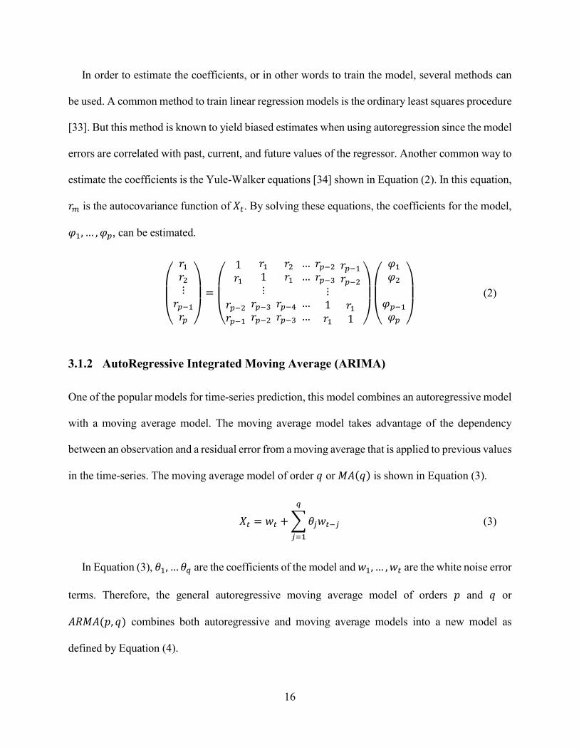
estimate the coefficients is the Yule-Walker equations [34] shown in Equation (2). In this equation,

𝑟𝑚 is the autocovariance function of 𝑋𝑡. By solving these equations, the coefficients for the model,

𝜑1, … , 𝜑𝑝, can be estimated.

(

𝑟1𝑟2⋮𝑟𝑝−1𝑟𝑝 )

=

(

1𝑟1

𝑟𝑝−2 𝑟𝑝−1

𝑟11⋮


𝑟2𝑟1


… … … …


⋮1𝑟1

𝑟𝑝−1𝑟𝑝−2 𝑟11

)

(

𝜑1𝜑2

𝜑𝑝−1𝜑𝑝 )

(2)

3.1.2 AutoRegressive Integrated Moving Average (ARIMA)

One of the popular models for time-series prediction, this model combines an autoregressive model

with a moving average model. The moving average model takes advantage of the dependency

between an observation and a residual error from a moving average that is applied to previous values

in the time-series. The moving average model of order 𝑞 or 𝑀𝐴(𝑞) is shown in Equation (3).

𝑋𝑡 = 𝑤𝑡 +∑𝜃𝑗𝑤𝑡−𝑗

𝑞

𝑗=1

(3)

In Equation (3), 𝜃1, … 𝜃𝑞 are the coefficients of the model and 𝑤1, … , 𝑤𝑡 are the white noise error

terms. Therefore, the general autoregressive moving average model of orders 𝑝 and 𝑞 or

𝐴𝑅𝑀𝐴(𝑝, 𝑞) combines both autoregressive and moving average models into a new model as

defined by Equation (4).

17

𝑋𝑡 =∑𝜑𝑗𝑋𝑡−𝑗

𝑝

𝑗=1

+∑𝜃𝑗𝑤𝑡−𝑗

𝑞

𝑗=1

+ 𝑤𝑡 (4)

The ARIMA model is a generalization of the ARMA model and is defined by Equation (5). In

this equation, the degree of differencing, d, is the number of times the data have had its past values

subtracted. B is the lag operator that is used to access previous observations using the formula

𝐵𝑘𝑋𝑡 = 𝑋𝑡−𝑘 . The coefficients for this model can be obtained using the smoothed periodogram

method [35].

(1 −∑𝜑𝑗𝑋𝑡−𝑗

𝑝

𝑗=1

) (1 − 𝐵)𝑑𝑋𝑡 = (1 +∑𝜃𝑗𝑤𝑡−𝑗

𝑞

𝑗=1

)𝑤𝑡 (5)

3.1.3 Exponential Smoothing

Even though it’s not usually considered to be a popular model for time-series prediction, it has been

used successfully in the past for time-series prediction in financial markets [33] [34]. Exponential

smoothing predicts future values by calculating the weighted average of past observations, with the

weights decaying exponentially as it gets to older observations. The exponential smoothing model

is defined in Equation (6) where 𝛼 is the smoothing constant, a value from 0 to 1, and 𝑆𝑡 is the

smoothed statistic. When 𝛼 is close to zero, the smoothing happens more slowly and the model

gives greater weight to older observations in the data. The best value for 𝛼 is the one that results in

the smallest mean squared error for the data. A popular method to find the optimal value of 𝛼 is the

Levenberg–Marquardt algorithm [38].

𝑆𝑡 = 𝛼𝑋𝑡 + (1 − 𝛼)𝑆𝑡−1 (6)

18

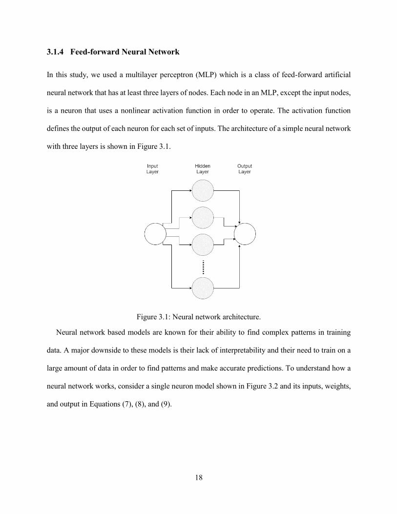
3.1.4 Feed-forward Neural Network

In this study, we used a multilayer perceptron (MLP) which is a class of feed-forward artificial

neural network that has at least three layers of nodes. Each node in an MLP, except the input nodes,

is a neuron that uses a nonlinear activation function in order to operate. The activation function

defines the output of each neuron for each set of inputs. The architecture of a simple neural network

with three layers is shown in Figure 3.1.

Figure 3.1: Neural network architecture.

Neural network based models are known for their ability to find complex patterns in training

data. A major downside to these models is their lack of interpretability and their need to train on a

large amount of data in order to find patterns and make accurate predictions. To understand how a

neural network works, consider a single neuron model shown in Figure 3.2 and its inputs, weights,

and output in Equations (7), (8), and (9).

19

Figure 3.2: Mathematical model if a single neuron.

𝑖𝑛𝑝𝑢𝑡 = 𝑋 = [𝑋0, 𝑋1, … , 𝑋𝑛] (7)

𝑤𝑒𝑖𝑔ℎ𝑡𝑠 = 𝜃 = [𝜃0, 𝜃1, … , 𝜃𝑛] (8)

𝑜𝑢𝑡𝑝𝑢𝑡 = ℎ(𝑥) = 𝑓(∑𝑋𝑘𝜃𝑘

𝑛

𝑘=0

) (9)

The dimension of the input is n – 1 since 𝑋0 is commonly used as the biased input. In order to

train the model, the weights, 𝜃, are initially set to a small value close to zero. When the input is sent

through the model, it is initially multiplied by the initial weights and the output is calculated based

on it. When the weighted sum of the input exceeds a predefined threshold value, the neuron outputs

a value which will be given to the activation function for mapping the value to the final output of

the neuron. This process is repeated for all neurons in the model, until the final output is calculated

in the output neuron. Based on the cost function associated with the model, if the calculated cost is

too high, backpropagation algorithm [39] is used to modify the weights of neurons with the goal of

decreasing the final cost.

20

3.1.5 Long Short-Term Memory

Recurrent Neural Network (RNN) is a category of artificial neural networks where connections

between nodes form a directed graph along a sequence which allows the network to exhibit dynamic

temporal behavior for a time sequence. Long short-term memory networks (LSTM) [35] are a

special kind of RNNs that are capable of learning long-term dependencies which makes them

suitable for time-series prediction, such as cryptocurrency price trends.

The main feature of LSTM networks is that each neuron can hold a state, with the ability to

remove or add information to the state as regulated by custom structures called gates. These gates

are built based on a sigmoid neural net layer and a pointwise multiplication operation. A sigmoid

layer outputs a value between zero and one which corresponds to the amount of each component

let through. An LSTM network contains three gates that regulate and control the state of the neuron.

The first step in an LSTM process is to decide what information to throw away from the cell

state. This decision is made by the forget gate based on the previous output and the current input.

The next step is to decide the new state of the neuron which is controlled by another gate called the

input gate based on the previous state and the new input. The final step is to calculate the final

output of the neuron by filtering the updated state. The output gate will make this decision based

on the updated state of the cell and the current input while keeping a copy of it for the next input.

3.2 Cryptocurrencies

In this study, we selected six different cryptocurrencies based on their popularity, availability of

historic price data, and market cap. These cryptocurrencies are Bitcoin, Ethereum, Bitcoin Cash,

Dash, Litecoin, and Monero. Table 3.1 presents these cryptocurrencies with their trading symbols,

number of data points, and the dates from which the data is included.

21

Table 3.1: List of selected cryptocurrencies

3.3 Dataset and Tools

The dataset for this study was obtained from Coin Metrics [41]. The dataset contains the closing

price history of 13 cryptocurrencies in comma-separated values format (CSV). The dataset is

updated daily from several exchanges and it contains some invalid data points that must be either

removed or fixed to make sure that models are working with proper data.

In order to read and use the dataset, Pandas framework [42] for Python programming language

is utilized. This framework reads a comma-separated values file and converts it to a DataFrame, a

two-dimensional heterogeneous tabular data structure, with the ability to iterate or breaking of the

file into chunks. After selecting relevant columns from the DataFrame, an algorithm was

implemented to iterate over and identify rows that contain missing or invalid data. With the help of

another dataset [43], many rows with either missing or invalid data were fixed. In rare cases were

22

both datasets didn’t have valid data for a row, that row and all previous rows were removed from

the dataset to make sure that models are built on continuous and valid data.

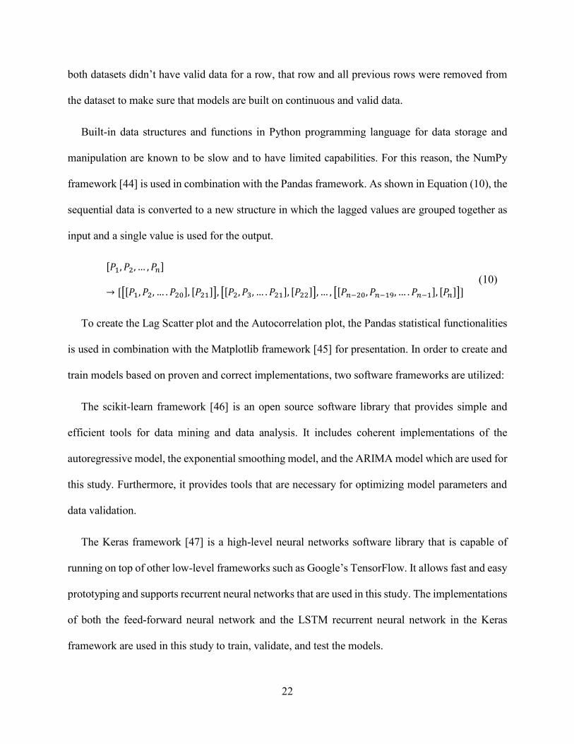
Built-in data structures and functions in Python programming language for data storage and

manipulation are known to be slow and to have limited capabilities. For this reason, the NumPy

framework [44] is used in combination with the Pandas framework. As shown in Equation (10), the

sequential data is converted to a new structure in which the lagged values are grouped together as

input and a single value is used for the output.

[𝑃1, 𝑃2, … , 𝑃𝑛]

→ [[[𝑃1, 𝑃2, … . 𝑃20], [𝑃21]], [[𝑃2, 𝑃3, … . 𝑃21], [𝑃22]],… , [[𝑃𝑛−20, 𝑃𝑛−19, … . 𝑃𝑛−1], [𝑃𝑛]]] (10)

To create the Lag Scatter plot and the Autocorrelation plot, the Pandas statistical functionalities

is used in combination with the Matplotlib framework [45] for presentation. In order to create and

train models based on proven and correct implementations, two software frameworks are utilized:

The scikit-learn framework [46] is an open source software library that provides simple and

efficient tools for data mining and data analysis. It includes coherent implementations of the

autoregressive model, the exponential smoothing model, and the ARIMA model which are used for

this study. Furthermore, it provides tools that are necessary for optimizing model parameters and

data validation.

The Keras framework [47] is a high-level neural networks software library that is capable of

running on top of other low-level frameworks such as Google’s TensorFlow. It allows fast and easy

prototyping and supports recurrent neural networks that are used in this study. The implementations

of both the feed-forward neural network and the LSTM recurrent neural network in the Keras

framework are used in this study to train, validate, and test the models.

Chapter 4

Results

After selecting models and preparing the data, we trained each model on the daily closing price data

for each cryptocurrency. We tried to optimize the parameters of each model to minimize the mean

squared error on our training data while preventing overfitting. Two performance metrics for each

model were measured: mean squared error and the accuracy of the model in predicting the direction

of price movement for the next day. To enable a meaningful comparison between the mean squared

error value among different cryptocurrencies, daily closing prices were normalized before being

used by the models.

4.1 Lag Scatter Plot

Since we have assumed that our observations have a relationship with the previous observations, it

is useful to explore the relationship using a lag scatter plot. In Figure 4.1, the scatter plot of six

cryptocurrencies are shown. In each plot, the horizontal axis indicates the price of the

cryptocurrency at time t and the vertical axis represents the price at t + 1. In all plots, points are

clustered along the diagonal line, indicating that there is a positive correlation relationship between

the closing price of a cryptocurrency and its lagged values.

24

Figure 4.1: Lag scatter plot of six cryptocurrencies.

25

4.2 Autocorrelation Plot

To quantify the strength and type of the relationship between prices with different lag values, the

autocorrelation plots of the selected cryptocurrencies are presented in Figure 4.2. The

autocorrelation number is a value between -1 and 1. The sign of this number indicates a negative or

positive correlation respectively. A value close to zero indicates a weak correlation, whereas a value

closer to 1 or -1 indicates a strong correlation.

By analyzing Figure 4.2, it is evident that there is a strong correlation among the most selected

cryptocurrencies for lag values less than 20. This value is useful in configuring the models,

especially the linear ones. Also, it is clear that there is no seasonality in our data and therefore there

is no need to remove it before feeding the data into our models.

26

Figure 4.2: Autocorrelation plot of six cryptocurrencies.

27

4.3 Performance and Discussion

In this section, the performance of each cryptocurrency is presented based on each model’s mean

squared error and price direction prediction accuracy. Accuracy is defined as the percentage of days

where each model has predicted the right price movement direction.

4.3.1 Bitcoin

The dataset for the daily price history of Bitcoin includes records from April 28th, 2013 to November

9th, 2018, with 2023 data points. The first 1923 data points were used for model training and

validation and the rest were used for testing.

Based on the results presented in Table 4.1, the lowest mean squared error rate among different

models is achieved by the ARIMA model, which outperforms all other models by this measurement.

The price direction prediction accuracy of the LSTM model is at 53% which is better than the

performance achieved by other models. Depending on the user goal, both the ARIMA model and

the LSTM model are suitable for the task of predicting the next-day price of Bitcoin.

Table 4.1: Bitcoin Results

28

4.3.2 Ethereum

The dataset for the daily price history of Ethereum includes records from August 7th, 2015 to

November 9th, 2018, with 1191 data points. The first 1091 data points were used for model training

and validation and the rest were used for testing.



The price direction prediction accuracy of the feed-forward neural network model is at 55% which

is better than the performance achieved by other models. Depending on the user goal, both the

ARIMA model and the feed-forward neural network model are suitable for the task of predicting

the next-day price of Ethereum.

Table 4.2: Ethereum Results

4.3.3 Bitcoin Cash

The dataset for the daily price history of Bitcoin Cash includes records from August 3rd, 2017 to

November 9th, 2018, with 464 data points. The first 364 data points are used for model training and

validation and the rest is used for testing.

29

Based on results presented in Table 4.3, the lowest mean squared error rate among different

models is achieved by the exponential smoothing model, which outperforms all other models by

this measurement. The price direction prediction accuracy of the ARIMA model is at 54% which is

better than the performance achieved by other models. Depending on the user goal, both the

ARIMA model and the exponential smoothing model are suitable for the task of predicting the next-

day price of Bitcoin Cash.

Table 4.3: Bitcoin Cash Results

4.3.4 Dash

The dataset for the daily price history of Dash includes records from February 14th, 2014 to





The price direction prediction accuracy of the LSTM model is at 57% which is better than the

performance achieved by other models. Depending on the user goal, both the ARIMA model and

the LSTM model are suitable for the task of predicting the next-day price of Dash cryptocurrency.

30

Table 4.4: Dash Results

4.3.5 Litecoin

The dataset for the daily price history of Litecoin includes records from April 28th, 2013 to




models is achieved by the feed-forward neural network model, which outperforms all other complex

models by this measurement. Also, the price direction prediction accuracy of this model is at 58%

which is better than the performance achieved by other models. Based on these observations, the

feed-forward neural network model is suitable for the task of predicting the next-day price of

Litecoin cryptocurrency.

31

Table 4.5: Litecoin Results

4.3.6 Monero

The dataset for the daily price history of Monero includes records from May 21st, 2014 to November

9th, 2018, with 1634 data points. The first 1534 data points were used for model training and

validation and the rest were used for testing.


models is achieved by the simple persistence model, which outperforms all other complex models

by this measurement. The price direction prediction accuracy of the ARIMA model is at 60% which

is better than the performance achieved by other models. Depending on the user goal, both the

ARIMA model and the simple persistence model are suitable for the task of predicting the next-day

price of Monero cryptocurrency.

32

Table 4.6: Monero Results

Chapter 5

Conclusion

Machine learning and the Blockchain technology have both attracted the attention of academics and

practitioners in recent years. Their applications in the real world are becoming increasingly visible

to everyone, from self-driving cars to anonymous cryptocurrency-based payment systems that are

commonly used worldwide. The goal of this study is to provide a better understanding of the

performance of common time-series prediction models on cryptocurrencies to researchers and

practitioners.

The results of the study presented in this thesis have several significant implications. First,

complex models for predicting the future prices of cryptocurrencies, and to a larger extent any

financial asset, are not always better than a simple persistence model. On average, the ARIMA

model has the best performance when measured by the mean squared error rate. When it comes to

predicting the direction of price movement, neural network-based models, such as LSTM, have a

better performance.

There are several areas of this study that can be expanded for future research. Utilizing more

data by using the intra-day prices of cryptocurrencies can give researchers new insights in this area.

Furthermore, applying other machine learning techniques that have not been investigated by this

34

study can be a great topic for future research. Some of these techniques are, but not limited to,

hidden Markov models, modular neural networks, and dynamic neural networks.

References

[1] S. Nakamoto, "Bitcoin: A Peer-to-Peer Electronic Cash System," 2008.

[2] "Coin Market Cap," [Online]. Available: https://coinmarketcap.com/currencies/bitcoin/.

[Accessed 16 06 2018].

[3] D. Bayer, S. Haber and W. S. Stornetta, "Improving the Efficiency and Reliability of Digital

Time-Stamping," in Springer, New York, NY, 1993.

[4] S. Haber and W. S. Stornetta, "How to time-stamp a digital document," Journal of Cryptology,

vol. 3, no. 2, pp. 99-111, 1991.

[5] "BigchainDB," [Online]. Available: bigchaindb.com. [Accessed 16 06 2018].

[6] "Namecoin," [Online]. Available: namecoin.org/. [Accessed 16 06 2018].

[7] "Steemit," [Online]. Available: steemit.com. [Accessed 16 06 2018].

[8] M. I. Jordan and T. M. Mitchell, "Machine learning: Trends, perspectives, and prospects,"

Science, vol. 349, no. 6245, pp. 255-260, 2017.

[9] "Machine Learning - Facebook Research," Facebook, [Online]. Available:

research.fb.com/category/machine-learning/. [Accessed 16 06 2018].

36

[10] T. Kimoto, K. Asakawa, M. Yoda and M. Takeoka, "Stock market prediction system with

modular neural networks," in IJCNN International Joint Conference on Neural Networks, San

Diego, 1990 .

[11] J. Zhai, Y. Cao and X. Ding, "Data analytic approach for manipulation detection in stock

market," Review of Quantitative Finance and Accounting, vol. 50, no. 3, pp. 897-932, 2018.

[12] M. Holub and J. Johnson, "Bitcoin research across disciplines," The Information Society, vol.

34, no. 2, pp. 114-126, 2018.

[13] A. Ashayer and N. Tabrizi, "Comprehensive Literature Review on Machine Learning

Techniques used in Blockchain Technology," Submitted to IEEE International Conference

on Blockchain , Atlanta, USA, 2019.

[14] D. Shah and K. Zhang, "Bayesian regression and Bitcoin," in 52nd Annual Allerton

Conference on Communication, Control, and Computing, Monticello, 2014.

[15] A. Greaves and B. Au, "Using the Bitcoin Transaction Graph to Predict the Price of Bitcoin,"

2015.

[16] S. Colianni, S. Rosales and M. Signorotti, "Algorithmic Trading of Cryptocurrency Based on

Twitter Sentiment Analysis," 2015.

[17] C. Lamon, E. Nielsen and E. Redondo, "Cryptocurrency Price Prediction Using News and

Social Media Sentiment," 2017.

37

[18] H. S. Yin and R. Vatrapu, "A first estimation of the proportion of cybercriminal entities in the

bitcoin ecosystem using supervised machine learning," in 2017 IEEE International

Conference on Big Data, Boston, 2017.

[19] B. Ly, D. Timaul, A. Lukanan, J. Lau and E. Steinmetz, "Applying Deep Learning to Better

Predict Cryptocurrency Trends," in Midwest Instruction and Computing Symposium, Duluth,

2018.

[20] S. Velankar, S. Valecha and S. Maji, "Bitcoin Price Prediction using Machine Learning," in

20th International Conference on Advanced Communication Technology, Chuncheon-si

Gangwon-do, 2018.

[21] Z. Jiang and J. Liang, "Cryptocurrency Portfolio Management with Deep Reinforcement

Learning," in Intelligent Systems Conference (IntelliSys), London, 2017.

[22] W. Chen, Z. Zheng, J. Cui, E. Ngai, P. Zheng and Y. Zhou, "Detecting Ponzi Schemes on

Ethereum: Towards Healthier Blockchain Technology," in World Wide Web Conference,

Lyon, 2018.

[23] S. McNally, J. Roche and S. Caton, "Predicting the Price of Bitcoin Using Machine Learning,"

in 26th Euromicro International Conference on Parallel, Distributed and Network-based

Processing (PDP), Cambridge, 2018.

[24] H. Jang and J. Lee, "An Empirical Study on Modeling and Prediction of Bitcoin Prices With

Bayesian Neural Networks Based on Blockchain Information," IEEE, vol. 6, pp. 5427-5437,

2017.

38

[25] N. Indera, I. Yassin, A. Zabidi and Z. Rizman, "Non-linear Autoregressive with Exogeneous

input (narx) bitcoin price prediction model using PSO-optimized parameters and moving

average technical indicators," Journal of Fundamental and Applied Sciences, vol. 9, no. 3S,

p. 791, 2018.

[26] Y. B. Kim, J. G. Kim, W. Kim, J. H. Im and T. Kim, "Predicting Fluctuations in

Cryptocurrency Transactions Based on User Comments and Replies," PLOS ONE, vol. 11,

no. 8, p. e0161197, 2016.

[27] L. Pichl and T. Kaizoji, "Volatility Analysis of Bitcoin Price Time Series," Quantitative

Finance and Economics, vol. 1, no. 4, pp. 474-485, 2017.

[28] M. Nakano, A. Takahashi and S. Takahashi, "Bitcoin Technical Trading With Artificial

Neural Network," 2018.

[29] L. Alessandretti, A. ElBahrawy, L. M. Aiello and A. Baronchelli, "Machine Learning the

Cryptocurrency Market," 2018.

[30] T. Guo and N. Antulov-Fantulin, "Predicting short-term Bitcoin price fluctuations from buy

and sell orders," 2018.

[31] T. R. Li, A. S. Chamrajnagar, X. R. Fong, N. R. Rizik and F. Fu, "Sentiment-Based Prediction

of Alternative Cryptocurrency Price Fluctuations Using Gradient Boosting Tree Model,"

2018..

[32] A. B. Kurtulmus and K. Daniel, "Trustless Machine Learning Contracts; Evaluating and

Exchanging Machine Learning Models on the Ethereum Blockchain," 2018.

39

[33] T.-T. Kuo and L. Ohno-Machado, "ModelChain: Decentralized Privacy-Preserving

Healthcare Predictive Modeling Framework on Private Blockchain Networks," 2018.

[34] A. Ashayer and N. Tabrizi, "Modeling and Prediction of Cryptocurrency Prices Using

Machine Learning Techniques," Submitted to IEEE Transactions on Services Computing,

2019.

[35] M. Stone and R. J. Brooks, "Continuum regression: cross-validated sequentially constructed

prediction embracing ordinary least squares, partial least squares and principal components

regression," Journal of the Royal Statistical Society: Series B (Methodological), vol. 52, no.

2, pp. 237-258, 1990.

[36] S. Theodoridis, "Chapter 1. Probability and Stochastic Processes," in Machine Learning: A

Bayesian and Optimization Perspective, Academic Press, 2015, pp. 9-51.

[37] V. A. Reisen, "Estimation of the fractional difference parameter in the ARIMA (p, d, q) model

using the smoothed periodogram," Journal of Time Series Analysis, vol. 15, no. 3, pp. 335-

350, 1994.

[38] M. Varga, "FORECASTING COMMODITY PRICES WITH EXPONENTIAL

SMOOTHING," E+M Ekonomie a Management, no. 3, pp. 94-97, 2008.

[39] J. I. Hansen, "Triple exponential smoothing; a tool for common stock price prediction,"

ProQuest Dissertations and Theses, p. 51, 1970.

[40] J. J. Moré, in The Levenberg-Marquardt algorithm: implementation and theory, Springer,

1978, pp. 105-116.

40

[41] R. Hecht-Nielsen, "Theory of the backpropagation neural network," in Neural networks for

perception, Elsevier, 1992, pp. 65-93.

[42] S. Hochreiter and J. Schmidhuber, "Long short-term memory," Neural computation, vol. 9,

no. 8, pp. 1735--1780, 1997.

[43] "Coin Metrics," [Online]. Available: https://coinmetrics.io/. [Accessed November 2018].

[44] "The Pandas Project," [Online]. Available: https://pandas.pydata.org/. [Accessed November

2018].

[45] "Bitcoin Charts," [Online]. Available: http://api.bitcoincharts.com/v1/csv/. [Accessed

November 2018].

[46] "NumPy," [Online]. Available: http://www.numpy.org/. [Accessed November 2018].

[47] "Matplotlib," [Online]. Available: https://matplotlib.org/. [Accessed November 2018].

[48] "scikit-learn," [Online]. Available: https://scikit-learn.org. [Accessed November 2018].

[49] "Keras," [Online]. Available: https://keras.io/. [Accessed November 2018].

[50] W. Koehrsen, "Introduction to Bayesian Linear Regression," [Online]. Available:

https://towardsdatascience.com/introduction-to-bayesian-linear-regression-e66e60791ea7.

[Accessed 16 7 2018].

[51] Y. LeCun, P. Haffner, L. Bottou and Y. Bengio, "Object recognition with gradient-based

learning," in Shape, contour and grouping in computer vision, Berlin, Heidelberg, Springer,

1999, pp. 319-345.

41

[52] R. Caruana, N. Karampatziakis and A. Yessenalina, "An empirical evaluation of supervised

learning in high dimensions," in ICML, 2008.

Alireza Ashayer April, 2019 Director of Thesis: Dr. Nasseh ...

Documents

Transcript of Alireza Ashayer April, 2019 Director of Thesis: Dr. Nasseh ...