1 INTRODUCTION

Algorithm Based Validation of a Simplified Elevator GroupController Model

Thomas Bartz–Beielstein∗ Sandor Markon† Mike Preuss∗

∗Universtitat DortmundD-44221 Dortmund, Germany

{tom,preuss}@LS11.cs.uni-dortmund.de

†FUJITEC Co.Ltd. World Headquarters28-10, Shoh 1-chome, Osaka, Japan

markon@rd.fujitec.co.jp

1 Introduction

Today’s urban life cannot be imagined without elevators. The central part of an elevatorsystem, the elevator group controller, assigns elevator cars to service calls in real-time whileoptimizing the overall service quality, the traffic throughput, and/or the energy consumption.The elevator supervisory group control (ESGC) problem can be classified as a combinato-rial optimization problem [Bar86, SC99, MN02]. It reveals the same complex behavior asmany other stochastic traffic control problems, i.e. materials handling systems (MHS) withautomated guided vehicles (AGVs).

Due to many difficulties in analysis, design, simulation, and control, the ESGC problemhas been studied for a long time. First approaches were mainly based on analytical approachesderived from queuing theory, whereas currently computational intelligence (CI) methods andother heuristics are accepted as state of the art [CB98, MN02, SWW02].

In this article we will propose a validation methodology for a simplified ESGC system, thesequential ring (S-ring). The S-ring is constructed as a simplified model of an ESGC systemusing a neural network (NN) to control the elevators. Some of the NN connection weights canbe modified, so that different weight settings and their influence on the ESGC performancecan be tested. The performance of one specific weight setting ~x is based on simulations ofspecific traffic situations, which automatically lead to stochastically disturbed (noisy) fitnessfunction values f(~x). The determination of an optimal weight setting ~x∗ is not trivial, since itis difficult to find an efficient strategy that modifies the weights without generating too manyinfeasible solutions, and to judge the performance or fitness f(~x) of one ESGC configuration.

The S-ring was introduced as a benchmark problem to enable a comparison of ESGCalgorithms, independently of specific elevator configurations [BFM00, Bey01]. Results from

1

CORE Metadata, citation and similar papers at core.ac.uk

Provided by Eldorado - Ressourcen aus und für Lehre, Studium und Forschung

2 2 THE ELEVATOR SUPERVISORY GROUP CONTROL PROBLEM

the S-ring, obtained with low computational costs, should be transferable to more complicateESGC models.

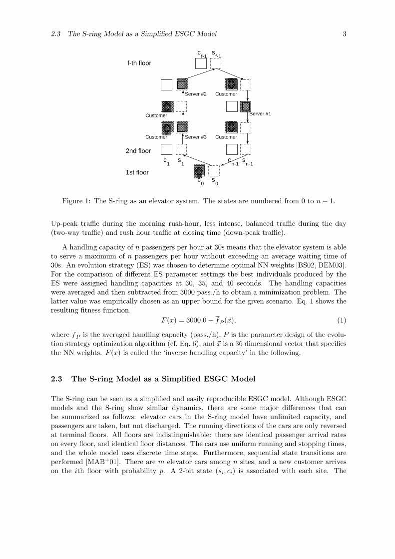
In the following, we will present different techniques to answer the question whether theS-ring is a simplified, but valid ESGC simulation model. We propose a new validation method-ology that takes the optimization algorithm for the simulation model into account. Tuning theoptimization algorithm on the simplified simulation model results in a good parameter settingfor the optimization algorithm, that is also applicable to the complex simulation model. Thus,improved algorithm parameter settings obtained from simulation results on the S-ring shouldbe transferable to real ESGC problems. S-ring simulations might give valuable hints for theoptimization of highly complex elevator group controller optimization tasks. The elements ofthis algorithm based validation method are shown in Fig. 2.

This paper is organized as follows: in Section 2, the ESGC problem is introduced. Section 3discusses different validation techniques. A concrete numerical example is presented in Sec. 4.Section 5 gives a summary and an outlook.

2 The Elevator Supervisory Group Control Problem

2.1 Elevator Control

We introduce one specific instance of the ESGC problem, a so-called destination call system.In traditional elevators customers can only press a button to request up or down service. Theychoose the exact destination after entering the elevator car. In a destination call system,the desired destination can be chosen at a terminal before entering the elevator car [BEM03].Fujitec, one of the world’s leading elevator manufacturers developed a controller that is trainedby use of a set of fuzzy controllers. Each controller represents control strategies for differenttraffic situations [Mar95]. The NN structure and the neural weights determine a concretecontrol strategy. The network structure as well as many of the weights remain fixed, onlysome of the weights on the output layer can be modified and optimized. A discrete-eventbased elevator group simulator is used to compute the controller’s performance. This ESGCsimulation model will be referred to as the ‘lift model’ (or simply ‘lift’) throughout the rest ofthis paper.

The identification of globally optimal weights is a highly complex task since the topologyof the fitness function is highly non-linear and highly multi-modal. It is stochastically dis-turbed due to the nondeterminism of service calls, and dynamically changing with respect totraffic loads. Gradient based optimization techniques cannot be applied successfully to thisoptimization problem. The computational effort for single simulator runs limits the maximumnumber of fitness function evaluations to the order of magnitude 104.

2.2 The Lift Model as an Optimization Problem

The objective function considered here is the average waiting time of all passengers servedduring a simulated elevator movement. Different traffic patterns occur during this simulation:

2.3 The S-ring Model as a Simplified ESGC Model 3

c0

s0

c1

s1

cn-1

sn-1

cf-1

sf-1

1st floor

2nd floor

f-th floor

Server #1

Server #2

Server #3Customer

Customer

Customer

Customer

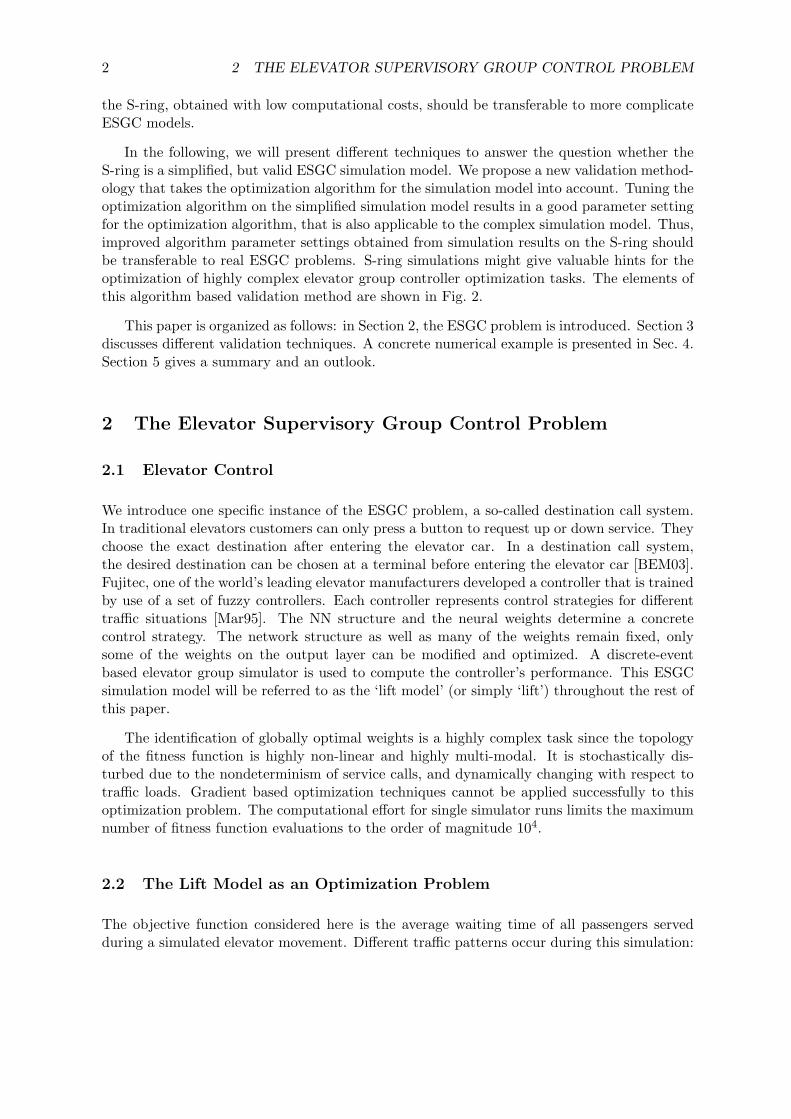
Figure 1: The S-ring as an elevator system. The states are numbered from 0 to n− 1.

Up-peak traffic during the morning rush-hour, less intense, balanced traffic during the day(two-way traffic) and rush hour traffic at closing time (down-peak traffic).

A handling capacity of n passengers per hour at 30s means that the elevator system is ableto serve a maximum of n passengers per hour without exceeding an average waiting time of30s. An evolution strategy (ES) was chosen to determine optimal NN weights [BS02, BEM03].For the comparison of different ES parameter settings the best individuals produced by theES were assigned handling capacities at 30, 35, and 40 seconds. The handling capacitieswere averaged and then subtracted from 3000 pass./h to obtain a minimization problem. Thelatter value was empirically chosen as an upper bound for the given scenario. Eq. 1 shows theresulting fitness function.

F (x) = 3000.0− fP (~x), (1)

where fP is the averaged handling capacity (pass./h), P is the parameter design of the evolu-tion strategy optimization algorithm (cf. Eq. 6), and ~x is a 36 dimensional vector that specifiesthe NN weights. F (x) is called the ‘inverse handling capacity’ in the following.

2.3 The S-ring Model as a Simplified ESGC Model

The S-ring can be seen as a simplified and easily reproducible ESGC model. Although ESGCmodels and the S-ring show similar dynamics, there are some major differences that canbe summarized as follows: elevator cars in the S-ring model have unlimited capacity, andpassengers are taken, but not discharged. The running directions of the cars are only reversedat terminal floors. All floors are indistinguishable: there are identical passenger arrival rateson every floor, and identical floor distances. The cars use uniform running and stopping times,and the whole model uses discrete time steps. Furthermore, sequential state transitions areperformed [MAB+01]. There are m elevator cars among n sites, and a new customer arriveson the ith floor with probability p. A 2-bit state (si, ci) is associated with each site. The

4 2 THE ELEVATOR SUPERVISORY GROUP CONTROL PROBLEM

Figure 2: Elements of algorithm based validation. The simplification of the complex model isvalid if the optimization algorithm reveals a similar behavior on the corresponding complexoptimization problem and the corresponding simplified problem.

following vector describes the state at time t of the S-ring:

[s0(t), c0(t), . . . , sn−1(t), cn−1(t)] ≡ x(t) ∈ X = {0, 1}2n.

The si bit is set to 1 if a server is present on the ith floor, otherwise it is set to 0. The sameapplies to the ci bits: they are set to 1 if at least one customer is waiting on the ith floor. Thesites are not updated synchronously, an updating cycle is decomposed into n steps as follows:The state evaluation is sequential, scanning the sites from n− 1 to 0, then again around fromn− 1. At each time step, one triplet ξ ≡ (ci, si, si+1) is updated, the updating being governedby the stochastic state transition rules, and by the ‘policy’ π : X → {0, 1}.

2.4 The S-Ring Model as an Optimization Problem

The S-ring model can be used to define an optimal control problem, by equipping it with anobjective function Q (here E is the expectation operator):

Q(n, m, p, π) = E(∑

ci

). (2)

Thus Q can be read as the expected number of floors with waiting customers. For givenparameters n, m, and p, the system evolution depends only on the policy π, thus this can bewritten as Q = Q(π). The optimal policy is defined as

π∗ = arg minπ

Q(π). (3)

5

The basic optimal control problem, referred to in the following as the S-ring optimizationproblem (S-ring problem), is to find π∗ for given parameters n, m, and p. The exact perfor-mance of a particular policy cannot be determined, it must be estimated. Problems related tooptimization via simulation are discussed in [BINN01].

3 The S-Ring Model as a Valid ESGC Model

In the following we will present standard validation techniques for simulation models. Wewill differentiate between model verification and model validation. Although verificationand validation of simulation models are related in some sense, we will consider validationonly [LK00, BINN01]. Classical validation processes are used to produce a model that repre-sents a given system behavior. This model should be accurate enough that it can be used asa representative of the real system.

We will extend these techniques by introducing a new approach, that takes the choice ofan optimization algorithm into account. Let the random variable Y denote the result of asimulation run or some measure of system performance in stochastic simulation. The goal of‘optimization via simulation’ is to minimize or maximize its expectation E(Y )[BINN01]. Weconsider optimization algorithms to define equivalence classes for optimization problems: anoptimization algorithm reveals the same behavior if applied to problems of the same equivalenceclass. Since the behavior of an optimization algorithm can be determined by running thesimulation, we can state: Simulation models are equivalent, if their corresponding optimizationproblems belong to the same equivalence class. Therefore we will distinguish models (e.g. the S-ring model) and their related problems (e.g. the S-ring problem). The validation of simulationmodels can be transfered to the question: are their corresponding optimization problemsequivalent?

3.1 Standard Validation Techniques

The complete validation process requires subjective and objective comparisons of the modelto the real system. Subjective comparisons are judgments of experts (‘face validity’), whereasobjective tests compare data generated by the model to data generated by the real system.We will discuss objective tests only, for subjective tests, the reader is referred to [BINN01].Building a model that has a high face validity, validating the model assumptions, and compar-ing the model input-output transformations to corresponding input-output transformationsfor the real system can be seen as three widely accepted steps of the validation process [NF67].In the following we will consider input-output transformations only. The model is viewed asthe function:

f : (X, D) → Y (4)

Thus values of the uncontrollable input parameters X and values of the controllable decisionvariables (or of the policy) D are mapped to the output measures Y .

The model can be run using generated random variates Xi to produce the simulation-generated output measures. E.g. the S-ring model takes a policy and a system configuration

6 3 THE S-RING MODEL AS A VALID ESGC MODEL

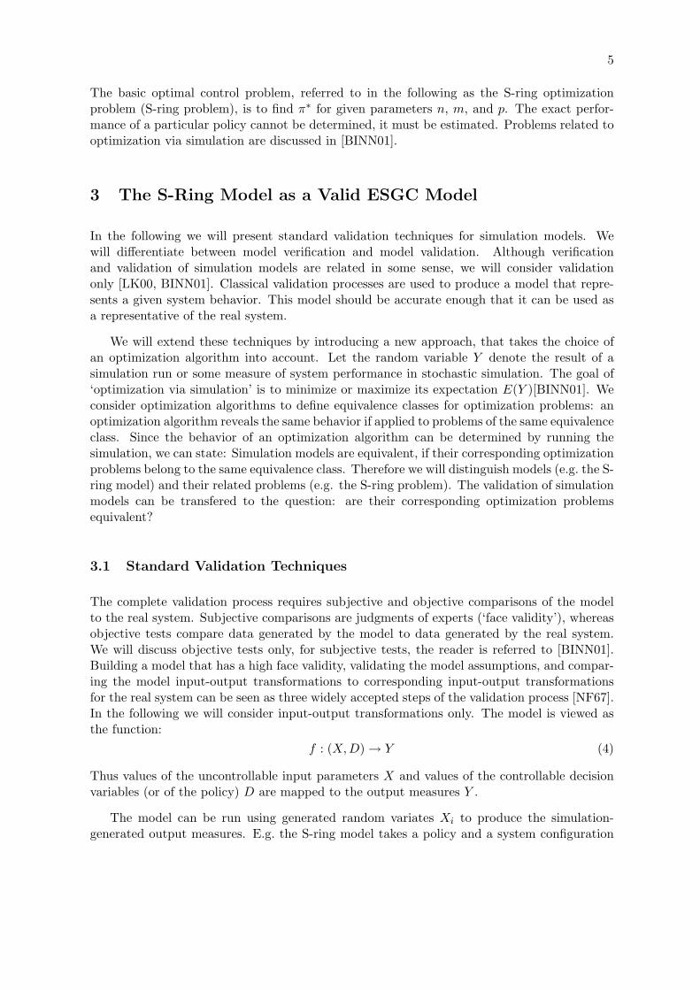
Table 1: DoE parameter setting for ESSymbol Parameter Typical Values Low Medium High

µ number of parent indi-viduals

10 . . . 100 5 12 19

ν = λ/µ offspring-parent ratio 1 . . . 10 2 4 6nσ number of standard

deviations1 . . . D - 1 -

τ0 global mutation pa-rameter

1/√

2√

D - 1/√

2√

D -

τi individual mutationparameter

1/√

2D - 1/√

2D -

κ age 1 . . .∞ 1 ∞ρ mixing number µ - 2 -R1 recombination opera-

tor for object vari-ables

{discrete} - {discrete} -

R2 recombination opera-tor for strategy vari-ables

{intermediate} - {intermediate} -

and determines the expected average number of floors with waiting customers in the systemusing the generated random variates that determine a customer arrival event.

If real system data is available, a statistical test of the null hypothesis can be conducted:

H0 : E(Y ) = µ is tested against H1 : E(Y ) 6= µ, (5)

where µ denotes the real system response and Y the simulated model response.

3.2 Algorithm Based Validation

Our goal is to show that the S-ring model is a valid ESGC-model. The first step in thealgorithm based validation (ABV) approach requires the selection of an optimization algorithm.Evolution strategies (ES), that are applicable to many optimization problems, have been chosenin the following [BS02]. Our approach is based on the assumption that specific problemsrequire specific algorithm parameter settings [WM97]. Algorithm based validation (ABV) isrelated to parameter tuning, but has to be distinguished from parameter control [EHM99].Parameter control deals with parameter values that are changed during the optimization run,whereas parameter tuning refers to exogenous algorithm parameters to be selected before theoptimization run is started [BS02]. Including the optimization algorithm into the validationprocess, we propose the following methodology [FL01]:

I. Tuning: The parameter setting of an optimization algorithm for one specific problem canbe tuned in the following manner [Bei03]. The S-ring simulation output is the expectedaverage number of floors with waiting customers (minimization problem). Therefore, wecan define the performance Q of a policy π for a given S-ring setting S := (n, m, p) ∈ S

3.2 Algorithm Based Validation 7

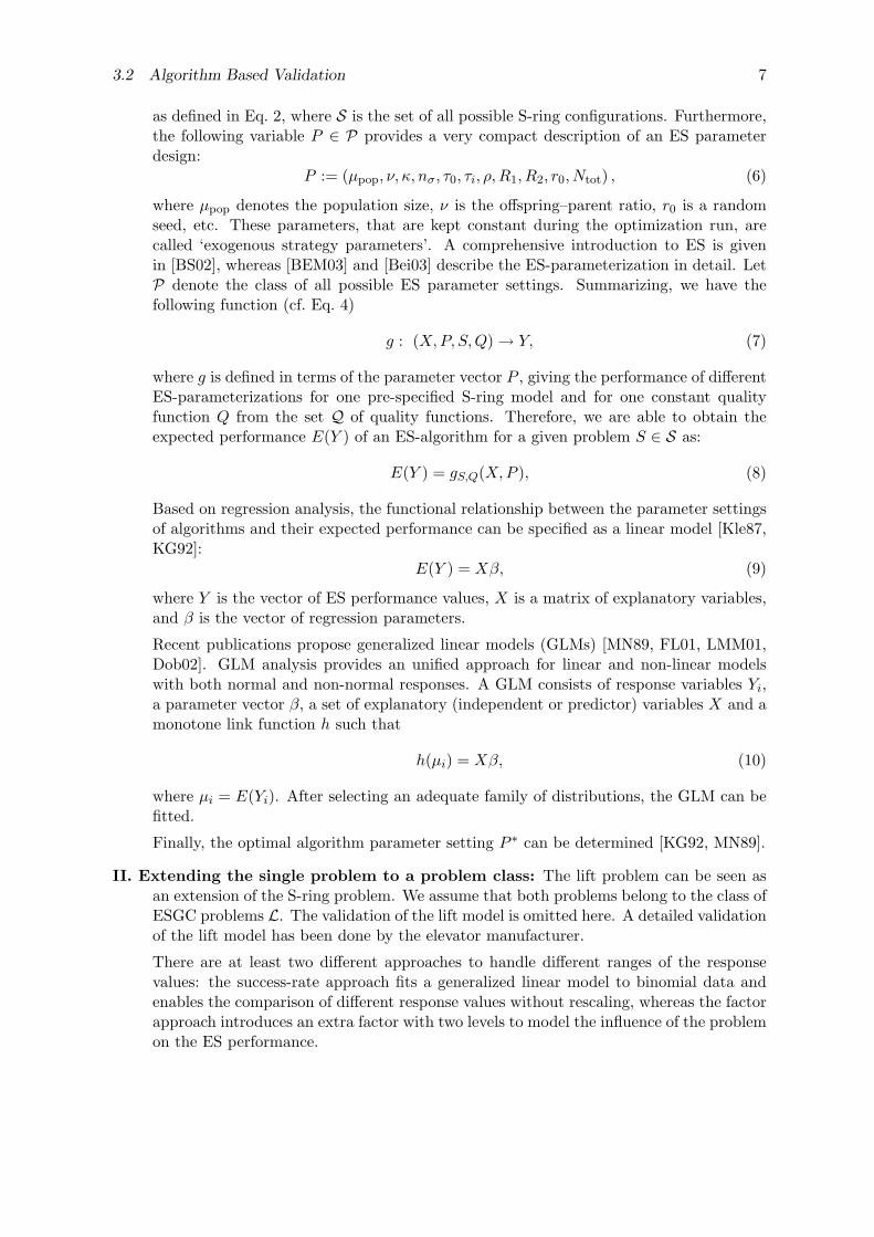
as defined in Eq. 2, where S is the set of all possible S-ring configurations. Furthermore,the following variable P ∈ P provides a very compact description of an ES parameterdesign:

P := (µpop, ν, κ, nσ, τ0, τi, ρ, R1, R2, r0, Ntot) , (6)

where µpop denotes the population size, ν is the offspring–parent ratio, r0 is a randomseed, etc. These parameters, that are kept constant during the optimization run, arecalled ‘exogenous strategy parameters’. A comprehensive introduction to ES is givenin [BS02], whereas [BEM03] and [Bei03] describe the ES-parameterization in detail. LetP denote the class of all possible ES parameter settings. Summarizing, we have thefollowing function (cf. Eq. 4)

g : (X, P, S, Q) → Y, (7)

where g is defined in terms of the parameter vector P , giving the performance of differentES-parameterizations for one pre-specified S-ring model and for one constant qualityfunction Q from the set Q of quality functions. Therefore, we are able to obtain theexpected performance E(Y ) of an ES-algorithm for a given problem S ∈ S as:

E(Y ) = gS,Q(X, P ), (8)

Based on regression analysis, the functional relationship between the parameter settingsof algorithms and their expected performance can be specified as a linear model [Kle87,KG92]:

E(Y ) = Xβ, (9)

where Y is the vector of ES performance values, X is a matrix of explanatory variables,and β is the vector of regression parameters.

Recent publications propose generalized linear models (GLMs) [MN89, FL01, LMM01,Dob02]. GLM analysis provides an unified approach for linear and non-linear modelswith both normal and non-normal responses. A GLM consists of response variables Yi,a parameter vector β, a set of explanatory (independent or predictor) variables X and amonotone link function h such that

h(µi) = Xβ, (10)

where µi = E(Yi). After selecting an adequate family of distributions, the GLM can befitted.

Finally, the optimal algorithm parameter setting P ∗ can be determined [KG92, MN89].

II. Extending the single problem to a problem class: The lift problem can be seen asan extension of the S-ring problem. We assume that both problems belong to the class ofESGC problems L. The validation of the lift model is omitted here. A detailed validationof the lift model has been done by the elevator manufacturer.

There are at least two different approaches to handle different ranges of the responsevalues: the success-rate approach fits a generalized linear model to binomial data andenables the comparison of different response values without rescaling, whereas the factorapproach introduces an extra factor with two levels to model the influence of the problemon the ES performance.

8 3 THE S-RING MODEL AS A VALID ESGC MODEL

(−1,−1) (−1,1)

(−a,0) (0,0) (a,0)

(1,1)(−1,1)

(0,a)

(0,−a)

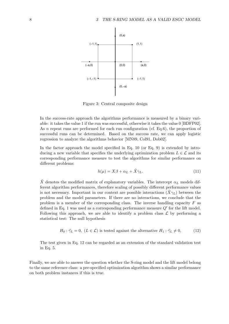
Figure 3: Central composite design

In the success-rate approach the algorithms performance is measured by a binary vari-able: it takes the value 1 if the run was successful, otherwise it takes the value 0 [BDFP02].As n repeat runs are performed for each run configuration (cf. Eq.6), the proportion ofsuccessful runs can be determined. Based on the success rate, we can apply logisticregression to analyze the algorithms behavior [MN89, Col91, Dob02].

In the factor approach the model specified in Eq. 10 (or Eq. 9) is extended by intro-ducing a new variable that specifies the underlying optimization problem L ∈ L and itscorresponding performance measure to test the algorithms for similar performance ondifferent problems:

h(µ) = Xβ + αL + XγL. (11)

X denotes the modified matrix of explanatory variables. The intercept αL models dif-ferent algorithm performances, therefore scaling of possibly different performance valuesis not necessary. Important in our context are possible interactions (XγL) between theproblem and the model parameters. If there are no interactions, we conclude that theproblem is a member of the corresponding class. The inverse handling capacity F asdefined in Eq. 1 was used as a corresponding performance measure Q′ for the lift model.Following this approach, we are able to identify a problem class L by performing astatistical test: The null hypothesis

H0 : ~γL = 0, (L ∈ L) is tested against the alternative H1 : ~γL 6= 0, (12)

The test given in Eq. 12 can be regarded as an extension of the standard validation testin Eq. 5.

Finally, we are able to answer the question whether the S-ring model and the lift model belongto the same reference class: a pre-specified optimization algorithm shows a similar performanceon both problem instances if this is true.

9

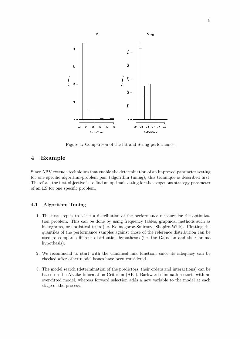
Figure 4: Comparison of the lift and S-ring performance.

4 Example

Since ABV extends techniques that enable the determination of an improved parameter settingfor one specific algorithm-problem pair (algorithm tuning), this technique is described first.Therefore, the first objective is to find an optimal setting for the exogenous strategy parameterof an ES for one specific problem.

4.1 Algorithm Tuning

1. The first step is to select a distribution of the performance measure for the optimiza-tion problem. This can be done by using frequency tables, graphical methods such ashistograms, or statistical tests (i.e. Kolmogorov-Smirnov, Shapiro-Wilk). Plotting thequantiles of the performance samples against those of the reference distribution can beused to compare different distribution hypotheses (i.e. the Gaussian and the Gammahypothesis).

2. We recommend to start with the canonical link function, since its adequacy can bechecked after other model issues have been considered.

3. The model search (determination of the predictors, their orders and interactions) can bebased on the Akaike Information Criterion (AIC). Backward elimination starts with anover-fitted model, whereas forward selection adds a new variable to the model at eachstage of the process.

10 4 EXAMPLE

4. From the final model we get estimates of the regression coefficients that are used todetermine an improved strategy parameter setting P ∗.

A numerical example will be given in the next subsection to demonstrate how parameter tuningcan be extended to study equivalence classes.

Table 2: Output generated in R for the GLM, Sec. 4.2Estimate Std. Error t value Pr(>|t|)

(Intercept) 0.4014 0.0017 231.75 0.0000Lift −0.3715 0.0011 −353.50 0.0000

P:poly(R, 2)1 −0.0002 0.0019 −0.10 0.9202P:poly(R, 2)2 0.0009 0.0010 0.86 0.3891

R:K-1 −0.0022 0.0004 −5.62 0.0000R:K1 −0.0000 0.0004 −0.01 0.9889

R:poly(P, 2)1 −0.0009 0.0035 −0.26 0.7967R:poly(P, 2)2 −0.0109 0.0024 −4.61 0.0000

poly(R, 2)1:K1 0.0157 0.0219 0.72 0.4735poly(R, 2)2:K1 −0.0191 0.0191 −1.00 0.3183

P:R:K-1 0.0001 0.0000 7.11 0.0000

4.2 Equivalence Classes for Problems

A central composite design (CCD) depictured in Fig. 3 was used to set up the experiments. Thecorresponding ES parameter settings are shown in Tab. 1. Histograms of the best fitness valueobtained during an optimization run can be used as a starting point to answer the questionwhether two problems L1 and L2 are in the same equivalence class. The histograms of theperformance function for the lift and the S-ring problem are shown in Fig. 4. Both histogramsshow assymetric empirical distributions that appear similar. Therefore a generalized linearmodel that is based on the Gamma distribution and the canonical link is used in the followinganalysis. A factor L with two levels {Sring, Lift} is introduced to check for interactions betweenalgorithm parameters and L. The model algebra introduced by Wilkinson and Rogers will beused to describe the regression model [WR73]: A+B+A:B reads ‘effect of factor A plus effect offactor B plus interaction between A and B’ and can be abbreviated as A*B. Starting from theoverfitted model with three factor interactions we perform a backward elimination procedure.The function stepAIC provided by the statistical software package R was used to automate thefirst steps in the process of model selection. R’s dropterm function was used to select significantterms manually. If P denotes the number of parent individuals, R the parent-offspring ratio,and K the age, the final model reads

Y ∼ Function + P : poly(R, 2) + R : K + R : poly(P, 2) + K : poly(R, 2) + P : R : K, (13)

and will be written in the following as Y ∼ Function+ model. The model coefficients, thatcan be used for algorithm tuning, are shown in Tab. 2. The last column in Tab. 2 shows thatthere are no significant interactions between the problem L and other factors.

11

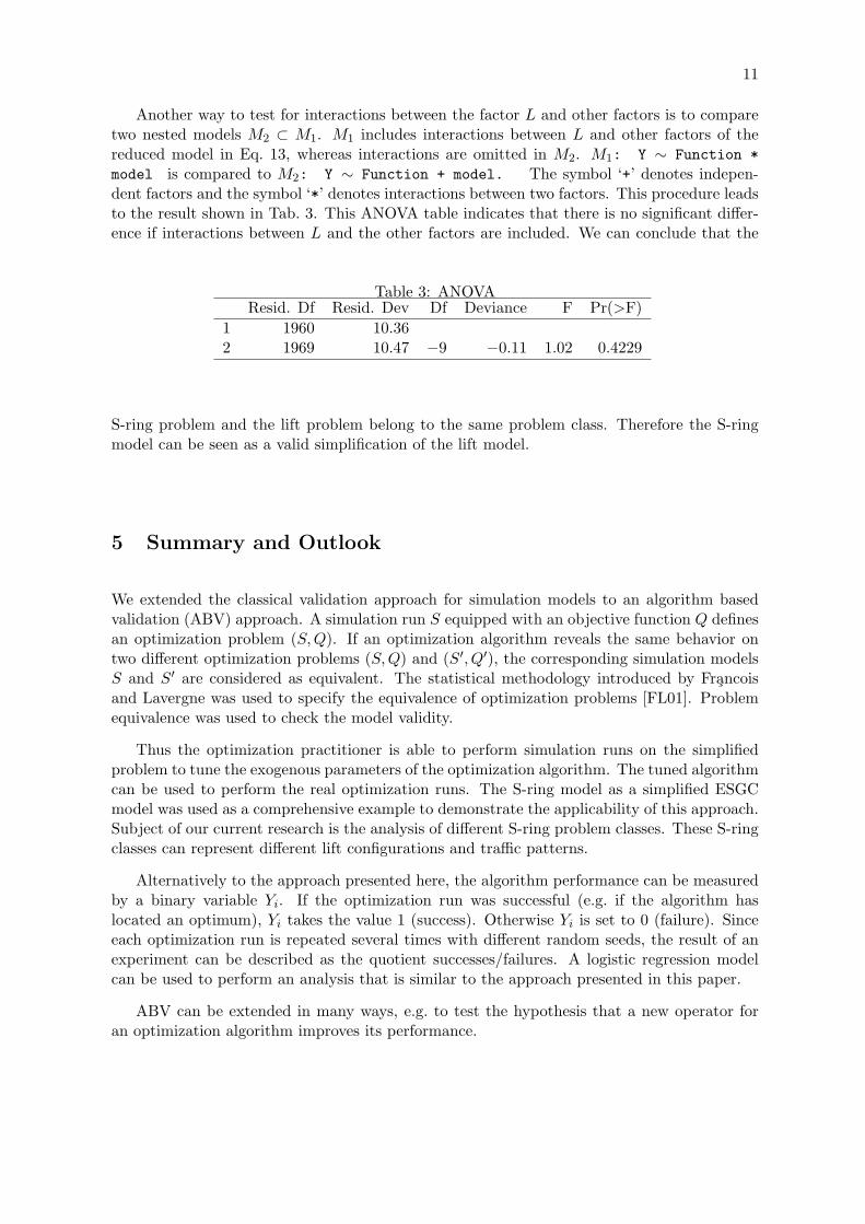
Another way to test for interactions between the factor L and other factors is to comparetwo nested models M2 ⊂ M1. M1 includes interactions between L and other factors of thereduced model in Eq. 13, whereas interactions are omitted in M2. M1: Y ∼ Function *model is compared to M2: Y ∼ Function + model. The symbol ‘+’ denotes indepen-dent factors and the symbol ‘*’ denotes interactions between two factors. This procedure leadsto the result shown in Tab. 3. This ANOVA table indicates that there is no significant differ-ence if interactions between L and the other factors are included. We can conclude that the

Table 3: ANOVAResid. Df Resid. Dev Df Deviance F Pr(>F)

1 1960 10.362 1969 10.47 −9 −0.11 1.02 0.4229

S-ring problem and the lift problem belong to the same problem class. Therefore the S-ringmodel can be seen as a valid simplification of the lift model.

5 Summary and Outlook

We extended the classical validation approach for simulation models to an algorithm basedvalidation (ABV) approach. A simulation run S equipped with an objective function Q definesan optimization problem (S, Q). If an optimization algorithm reveals the same behavior ontwo different optimization problems (S, Q) and (S′, Q′), the corresponding simulation modelsS and S′ are considered as equivalent. The statistical methodology introduced by Francoisand Lavergne was used to specify the equivalence of optimization problems [FL01]. Problemequivalence was used to check the model validity.

Thus the optimization practitioner is able to perform simulation runs on the simplifiedproblem to tune the exogenous parameters of the optimization algorithm. The tuned algorithmcan be used to perform the real optimization runs. The S-ring model as a simplified ESGCmodel was used as a comprehensive example to demonstrate the applicability of this approach.Subject of our current research is the analysis of different S-ring problem classes. These S-ringclasses can represent different lift configurations and traffic patterns.

Alternatively to the approach presented here, the algorithm performance can be measuredby a binary variable Yi. If the optimization run was successful (e.g. if the algorithm haslocated an optimum), Yi takes the value 1 (success). Otherwise Yi is set to 0 (failure). Sinceeach optimization run is repeated several times with different random seeds, the result of anexperiment can be described as the quotient successes/failures. A logistic regression modelcan be used to perform an analysis that is similar to the approach presented in this paper.

ABV can be extended in many ways, e.g. to test the hypothesis that a new operator foran optimization algorithm improves its performance.

12 REFERENCES

References

[Bar86] G. Barney. Elevator Traffic Analysis, Design and Control. Cambridg U.P., 1986.

[BDFP02] T. Beielstein, J. Dienstuhl, C. Feist, and M. Pompl. Circuit design using evolu-tionary algorithms. In David B. Fogel, Mohamed A. El-Sharkawi, Xin Yao, GarryGreenwood, Hitoshi Iba, Paul Marrow, and Mark Shackleton, editors, Proceedingsof the 2002 Congress on Evolutionary Computation CEC2002, pages 1904–1909.IEEE Press, 2002.

[Bei03] T. Beielstein. Tuning evolutionary algorithms. Technical Report 148/03, Univer-sitat Dortmund, 2003.

[BEM03] T. Beielstein, C.P. Ewald, and S. Markon. Optimal elevator group controlby evolution strategies. In Proc. 2003 Genetic and Evolutionary ComputationConf. (GECCO’03), Chicago, Berlin, 2003. Springer.

[Bey01] H.-G. Beyer. The Theory of Evolution Strategies. Natural Computing Series.Springer, Heidelberg, 2001.

[BFM00] Th. Back, D. B. Fogel, and Z. Michalewicz, editors. Evolutionary Computation 1– Basic Algorithms and Operators. Institute of Physics Publ., Bristol, 2000.

[BINN01] J. Banks, J. S. Carson II, B. L. Nelson, and D. M. Nicol. Discrete Event SystemSimulation. Prentice Hall, 2001.

[BS02] H.-G. Beyer and H.-P. Schwefel. Evolution strategies – A comprehensive introduc-tion. Natural Computing, 1:3–52, 2002.

[CB98] R.H. Crites and A.G. Barto. Elevator group control using multiple reinforcementlearning agents. Machine Learning, 33(2-3):235–262, 1998.

[Col91] D. Collett. Modelling Binary Data. Chapman and Hall, 1991.

[Dob02] A.J. Dobson. An Introduction to Generalized Linear Models. Chapman and Hall,2nd edition, 2002.

[EHM99] A.E. Eiben, R. Hinterding, and Z. Michalewicz. Parameter control in evolutionaryalgorithms. IEEE Trans. on Evolutionary Computation, 3(2):124–141, 1999.

[FL01] O. Francois and C. Lavergne. Design of evolutionary algorithms – a statisticalperspective. IEEE Transactions on Evolutionary Computation, 5(2):129–148, April2001.

[KG92] J. .P. C. Kleijnen and W. Van Groenendaal. Simulation - A Statistical Perspective.Wiley, Chichester, 1992.

[Kle87] J. Kleijnen. Statistical Tools for Simulation Practitioners. Marcel Dekker, NewYork, 1987.

[LK00] A.M. Law and W.D. Kelton. Simulation Modelling and Analysis. McGraw-HillSeries in Industrial Egineering and Management Science. McGraw-Hill, New York,3rd edition, 2000.

REFERENCES 13

[LMM01] S.L. Lewis, D.C. Montgomery, and R.H. Myers. Examples of designed experimentswith nonnormal responses. Journal of Quality Technology, 33(3):265–278, July2001.

[MAB+01] S. Markon, D.V. Arnold, T. Back, T. Beielstein, and H.-G. Beyer. Thresholding– a selection operator for noisy ES. In J.-H. Kim, B.-T. Zhang, G. Fogel, andI. Kuscu, editors, Proc. 2001 Congress on Evolutionary Computation (CEC’01),pages 465–472, Seoul, Korea, May 27–30, 2001. IEEE Press, Piscataway NJ.

[Mar95] S. Markon. Studies on Applications of Neural Networks in the Elevator System.PhD thesis, Kyoto University, 1995.

[MN89] P. McCullagh and J.A. Nelder. Generalized Linear Models. Chapman and Hall,2nd edition, 1989.

[MN02] S. Markon and Y. Nishikawa. On the analysis and optimization of dynamic cellularautomata with application to elevator control. In The 10th Japanese-GermanSeminar, Nonlinear Problems in Dynamical Systems, Theory and Applications.unknown, Noto Royal Hotel, Hakui, Ishikawa, Japan, September 2002.

[NF67] T.H. Naylor and J.M. Finger. Verification of computer simulation models. Man-agement Science, 2:B92–B101, 1967.

[SC99] A.T. So and W.L. Chan. Intelligent Building Systems. Kluwer A.P., 1999.

[SWW02] H.-P. Schwefel, I. Wegener, and K. Weinert, editors. Advances in ComputationalIntelligence – Theory and Practice. Natural Computing Series. Springer, Berlin,2002.

[WM97] D.H. Wolpert and W.G. Macready. No free lunch theorems for optimization. IEEETransactions on Evolutionary Computation, 1(1):67–82, 1997.

[WR73] G. N. Wilkinson and C. E. Rogers. Symbolic description of factorial models foranalysis of variance. 22(3):392–399, 1973.