Simplified Parallel Domain Traversal

Wesley Kendall∗, Jingyuan Wang∗, Melissa Allen†, Tom Peterka‡, Jian Huang∗, andDavid Erickson§

∗ Department of Electrical Engineering and Computer Science, The University of Tennessee, Knoxville† Department of Civil and Environmental Engineering, The University of Tennessee, Knoxville

‡ Mathematics and Computer Science Division, Argonne National Laboratory§ Computational Earth Sciences Group, Oak Ridge National Laboratory

ABSTRACTMany data-intensive scientific analysis techniques requireglobal domain traversal, which over the years has beena bottleneck for efficient parallelization across distributed-memory architectures. Inspired by MapReduce and othersimplified parallel programming approaches, we have de-signed DStep, a flexible system that greatly simplifies effi-cient parallelization of domain traversal techniques at scale.In order to deliver both simplicity to users as well as scalabil-ity on HPC platforms, we introduce a novel two-tiered com-munication architecture for managing and exploiting asyn-chronous communication loads. We also integrate our de-sign with advanced parallel I/O techniques that operate di-rectly on native simulation output. We demonstrate DStepby performing teleconnection analysis across ensemble runsof terascale atmospheric CO2 and climate data, and we showscalability results on up to 65,536 IBM BlueGene/P cores.

KeywordsData-Intensive Analysis, Parallel Processing, Parallel Parti-cle Tracing, Atmospheric Ensemble Analysis

1. INTRODUCTIONDomain traversal is the ordered flow of information

through a data domain and the associated processing thataccompanies it. It is a series of relatively short-range andinterleaved communication/computation updates that ulti-mately results in a quantity computed along a spatially- ortime-varying span. When the domain is partitioned amongprocessing elements in a distributed-memory architecture,domain traversal involves a large number of information ex-changes among nearby subdomains accompanied by localprocessing of information prior to, during, and after thoseexchanges. Examples include computing advection in flowvisualization; and global illumination, particle systems, scat-tering, and multiple scattering in volume visualization.

A capability to flexibly analyze scientific data using paral-lel domain traversal at scale is much needed but still funda-

Permission to make digital or hard copies of all or part of this work forpersonal or classroom use is granted without fee provided that copies arenot made or distributed for profit or commercial advantage and that copiesbear this notice and the full citation on the first page. To copy otherwise, torepublish, to post on servers or to redistribute to lists, requires prior specificpermission and/or a fee.SC11 November 12-18, 2011, Seattle, Washington, USACopyright 2011 ACM 978-1-4503-0771-0/11/11 ...$10.00.

mentally new to many application scientists. For example,in atmospheric science, the planet-wide multi-physics mod-els are becoming very complex. Yet, to properly evaluatethe significance of the global and regional change of anygiven variable, one must be able to identify impacts outsidethe immediate source region. One example is to quantifytransport mechanisms of climate models and associated in-teractions for CO2 emitted into the atmosphere at specificlocations in the global carbon cycle. Uncertainty quantifi-cation of ensemble runs is another example.

Parallelization of domain traversal techniques acrossdistributed-memory architectures is very challenging in gen-eral, especially when the traversal is data dependent. Forexample, numerical integration in flow advection dependson the result of the previous integration step. Such datadependency can make task parallelism the only option forparallel acceleration; however, at large scale (e.g. tens ofthousands of processes), when each particle trace could po-tentially traverse through the entire domain, one must dealwith complexities of managing dynamic parallelism of com-munication, work assignment, and load balancing.

In this work, we provide application scientists with a sim-plified mode of domain-traversal analysis in a general envi-ronment that transparently delivers superior scalability. Wecall our system DStep. In particular, we note DStep’s novelability to abstract and utilize asynchronous communication.Since today’s HPC machines commonly offer multiple net-work connections per node paired with direct memory access(DMA), asynchronous communication is a viable strategyfor hiding transfer time. Asynchronous exchanges, however,can easily congest a network at large process counts. Wefound that efficient buffer management paired with a two-tiered communication strategy enabled DStep to efficientlyoverlap communication and computation at large scale. Us-ing fieldline tracing as a test of scalability, DStep can ef-ficiently handle over 40 million particles on 65,536 cores, aproblem size over two orders of magnitude larger than recentstudies in 2009 [23] and 2011 [21].

Along with abstracting complicated I/O and communica-tion management, DStep also provides a greatly simplifiedprogramming environment that shares similar qualities asthose of MapReduce [7] for text processing and Pregel [19]for graph processing.

The simplicity of our approach paired with the scalableback end has allowed us to write succinct and expressivecustom data analysis applications using DStep. As a re-sult, atmospheric scientists have a new way to evaluate thelongitudinal dependence of inter-hemispheric transport; for

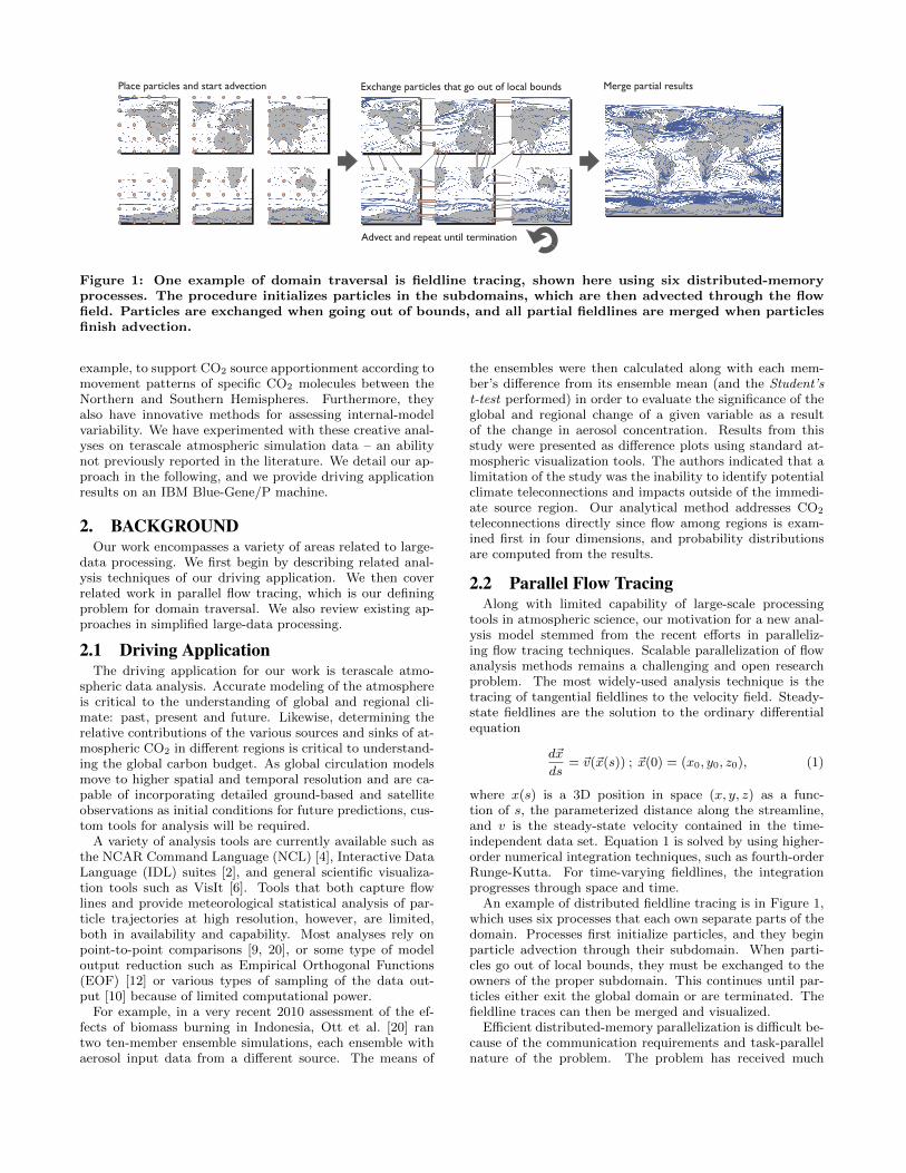
Exchange particles that go out of local bounds Merge partial results

Advect and repeat until termination

Place particles and start advection

Figure 1: One example of domain traversal is fieldline tracing, shown here using six distributed-memoryprocesses. The procedure initializes particles in the subdomains, which are then advected through the flowfield. Particles are exchanged when going out of bounds, and all partial fieldlines are merged when particlesfinish advection.

example, to support CO2 source apportionment according tomovement patterns of specific CO2 molecules between theNorthern and Southern Hemispheres. Furthermore, theyalso have innovative methods for assessing internal-modelvariability. We have experimented with these creative anal-yses on terascale atmospheric simulation data – an abilitynot previously reported in the literature. We detail our ap-proach in the following, and we provide driving applicationresults on an IBM Blue-Gene/P machine.

2. BACKGROUNDOur work encompasses a variety of areas related to large-

data processing. We first begin by describing related anal-ysis techniques of our driving application. We then coverrelated work in parallel flow tracing, which is our definingproblem for domain traversal. We also review existing ap-proaches in simplified large-data processing.

2.1 Driving ApplicationThe driving application for our work is terascale atmo-

spheric data analysis. Accurate modeling of the atmosphereis critical to the understanding of global and regional cli-mate: past, present and future. Likewise, determining therelative contributions of the various sources and sinks of at-mospheric CO2 in different regions is critical to understand-ing the global carbon budget. As global circulation modelsmove to higher spatial and temporal resolution and are ca-pable of incorporating detailed ground-based and satelliteobservations as initial conditions for future predictions, cus-tom tools for analysis will be required.

A variety of analysis tools are currently available such asthe NCAR Command Language (NCL) [4], Interactive DataLanguage (IDL) suites [2], and general scientific visualiza-tion tools such as VisIt [6]. Tools that both capture flowlines and provide meteorological statistical analysis of par-ticle trajectories at high resolution, however, are limited,both in availability and capability. Most analyses rely onpoint-to-point comparisons [9, 20], or some type of modeloutput reduction such as Empirical Orthogonal Functions(EOF) [12] or various types of sampling of the data out-put [10] because of limited computational power.

For example, in a very recent 2010 assessment of the ef-fects of biomass burning in Indonesia, Ott et al. [20] rantwo ten-member ensemble simulations, each ensemble withaerosol input data from a different source. The means of

the ensembles were then calculated along with each mem-ber’s difference from its ensemble mean (and the Student’st-test performed) in order to evaluate the significance of theglobal and regional change of a given variable as a resultof the change in aerosol concentration. Results from thisstudy were presented as difference plots using standard at-mospheric visualization tools. The authors indicated that alimitation of the study was the inability to identify potentialclimate teleconnections and impacts outside of the immedi-ate source region. Our analytical method addresses CO2

teleconnections directly since flow among regions is exam-ined first in four dimensions, and probability distributionsare computed from the results.

2.2 Parallel Flow TracingAlong with limited capability of large-scale processing

tools in atmospheric science, our motivation for a new anal-ysis model stemmed from the recent efforts in paralleliz-ing flow tracing techniques. Scalable parallelization of flowanalysis methods remains a challenging and open researchproblem. The most widely-used analysis technique is thetracing of tangential fieldlines to the velocity field. Steady-state fieldlines are the solution to the ordinary differentialequation

d�x

ds= �v(�x(s)) ; �x(0) = (x0, y0, z0), (1)

where x(s) is a 3D position in space (x, y, z) as a func-tion of s, the parameterized distance along the streamline,and v is the steady-state velocity contained in the time-independent data set. Equation 1 is solved by using higher-order numerical integration techniques, such as fourth-orderRunge-Kutta. For time-varying fieldlines, the integrationprogresses through space and time.

An example of distributed fieldline tracing is in Figure 1,which uses six processes that each own separate parts of thedomain. Processes first initialize particles, and they beginparticle advection through their subdomain. When parti-cles go out of local bounds, they must be exchanged to theowners of the proper subdomain. This continues until par-ticles either exit the global domain or are terminated. Thefieldline traces can then be merged and visualized.

Efficient distributed-memory parallelization is difficult be-cause of the communication requirements and task-parallelnature of the problem. The problem has received much

recent attention. Yu et al. [27] demonstrated visualiza-tion of pathlets, or short pathlines, across 256 Cray XTcores. Time-varying data were treated as a single 4D uni-fied dataset, and a static prepartitioning was performed todecompose the domain into regions that approximate theflow directions. The preprocessing was expensive, however,less than one second of rendering required approximately 15minutes to build the decomposition.

Pugmire et al. [23] took a different approach, opting toavoid the cost of preprocessing altogether. They chose acombination of static decomposition and out-of-core dataloading, directed by a master process that monitors loadbalance. They demonstrated results on up to 512 CrayXT cores, on problem sizes of approximately 20 K parti-cles. Data sizes were approximately 500 M structured gridcells, and the flow was steady.

Peterka et al. [21] avoided the bottleneck of having onemaster and instead used static and dynamic geometric par-titioning strategies for achieving desirable load balance. Theauthors showed that simple static round-robin partition-ing schemes outperformed dynamic partitioning schemes inmany cases because of the extra data movement overhead.They showed scalability results up to 32 K Blue Gene/Pcores on steady and time-varying datasets on problem sizesof approximately 120 K particles.

Because parallel particle tracing is one of the most well-defined domain traversal problems in visualization, we use itas the primary test case. However, beyond this test case, ouroverall goal is to create a design for general domain traver-sal problems. The novelty of our work is to improve usereffectiveness by allowing them to write succinct and pow-erful analysis applications, and by transparently acheivingscalability at large scale without the need of detailed under-standing of each parallel systems’ unique aspects. Hence,a comparison solely about performance against algorithmsmentioned in this section is beyond the scope of this work.

2.3 Simplified Large-Scale Data ProcessingMany large data processing problems have been solved

by allowing users to write serial functional programs whichcan be executed in parallel. The defining example isGoogle’s MapReduce [7], which provides a simple program-ming framework for data parallel tasks. Users implementa map() and reduce() function. The map() function takesan arbitrary input and outputs a list of intermediate [key,value] pairs. The reduce() function accepts a key and a listof values associated with the key. Reducers typically mergethe values, emitting one or zero outputs per key. Outputvalues can then be read by another MapReduce application,or by the same application (i.e. an iterative MapReduce).

While the programming interface is restricted, MapRe-duce provides a powerful abstraction that alleviates pro-gramming burdens by handling the details of data parti-tioning, I/O, and data shuffling. The power offered to usersby this abstraction has advocated new approaches at solv-ing large-scale problems in industrial settings [8]. There arealso systems that have implemented MapReduce on top ofMPI [13, 22] as well as multi-GPU architectures [25].

The profound success of MapReduce in industry has in-spired its use in scientific settings. Tu et al. [26] designed Hi-Mach, a Molecular Dynamics trajectory analysis frameworkbuilt on top of MapReduce. The authors extended the origi-nal MapReduce model to support multiple reduction phases

for various time-varying analysis tasks, and they showedscalability up to 512 cores on a Linux cluster. Kendall etal. [14] also performed time-varying climatic analysis taskson over a terabyte of satellite data using an infrastructuresimilar to MapReduce. The authors showed scalability up to16 K Cray XT4 cores and total end-to-end execution timesunder a minute.

Although MapReduce is useful for data-parallel tasks,many problems are not inherently data parallel and aredifficult to efficiently parallelize with MapReduce. Graphprocessing is one class of problems that fit in this cate-gory. Malewicz et al. introduced Pregel [19], a program-ming framework and implementation for processing large-scale graphs. In contrast with MapReduce, a process inPregel has the ability to communicate to neighbors basedon the topology of the graph. Users are required to imple-ment various functions that operate on a per-vertex basis.The authors showed that the model was expressive enoughto perform many popular graph algorithms, and to also scaleacross thousands of cores in a commodity cluster.

Like Pregel, we have found that allowing a restricted formof communication provides a much more flexible model fordata traversal. In contrast, DStep and our analysis needs arecentered around spatiotemporal scientific datasets. Allow-ing arbitrary traversal through a domain, while powerful formany tasks, can easily introduce high communication vol-umes that do not have a structured form such as a graph.

3. DSTEP - SIMPLIFIED PARALLEL DO-MAIN TRAVERSAL

Our analysis approach and implementation, DStep, isbuilt primarily on two functions: dstep() and reduce(). Thedstep() function is passed an arbitrary point in a spatiotem-poral domain. Given this point, steppers (those executingthe dstep() function) have immediate access to a localizedblock of the domain which surrounds the point. During theglobal execution of all steppers (the traversal phase), eachstepper has the ability to implicitly communicate with oneanother by posting generic data to a point in the domain.In contrast to MPI, where processes communicate to othersbased on rank, this abstraction is more intuitive for domaintraversal tasks, and it also allows for flexible integration intoa serial programming environment. In other words, DStepprograms do not have awareness of other processes.

The reduce() function is identical to that of MapReduce.We found that after the traversal phase, data-parallel oper-ations were important for many of our collaborators’ needs.For example, one operation is reducing lat-lon points to com-pute monthly averages and vertical distribution statistics.

3.1 DStep APIThe API of DStep promotes a similar design to that of

MapReduce. Users define functions that take arbitrary dataas input, and data movement is guided by emit functions.Two functions are defined by the user:

dstep(point, block, user data) – Takes a point tuple fromthe dataset ([x, y, z, t]), the enclosing block subdomain,and user data associated with the point.

reduce(key, user data[ ]) – Takes a key and list of associateduser data.

Three functions are called by the user program:

emit dstep(point, user data) – Takes a point tuple belong-ing to any part of the domain and arbitrary user data.The data is sent to the proper part of the domain,where it may continue traversal.

emit reduce(key, user data) – Takes a key and associateduser data. All user data values associated with a keyare sent to a reducer.

emit write(user data) – Takes arbitrary user data, which isstored to disk.

Using this API, the dstep() function of our fieldline tracingproblem shown in Figure 1 could be written as:

function dstep(point, block, user data)if user data.empty() then

user data.key = point � Key equals trace startuser data.trace size = 0 � Initialize trace size

end ifFieldline trace � Initialize partial fieldline tracewhile user data.trace size < MaxTraceSize do

trace.append(point)point = RK4(point, block) � Runge-Kuttauser data.trace size++if !block.contains(point) then

� Post new point when going out of boundsemit dstep(point, user data)break

end ifend whileemit reduce(user data.key, trace) � Partial result

end function

In this example, fieldlines are computed using fourth-order Runge-Kutta integration. During tracing, steppersemit points to other subdomains when tracing goes out ofbounds, and they also emit partial fieldlines for reduce().The reduce() function would then be responsible for merg-ing partial fieldlines (as shown in Figure 1).

The user data variable allows users to pass around arbi-trary data for analysis purposes. In fact – although not rec-ommended because of performance reasons – the user couldalso pass the entire computed fieldline to other steppers in-stead of reducing partial results.

3.2 DStep Application InstantiationThere are three aspects to instantiating a DStep appli-

cation, each of which can be controlled programmaticallyor by XML configuration files. The first is data input. Inthe spirit of designs such as MapReduce and NoSQL (i.e.avoiding data reorganization before analysis), DStep man-ages input of native application datasets. This ability hasbeen crucial to our user and application needs, which (inour case) has allowed us to abstract the management ofthousands of multi-variable netCDF files. Furthermore, wehave observed that our scientists are often only interestedin analyzing subsets of their datasets at a given time. Be-cause of this observation, which is common in many set-tings [24], we allow users to specify input as compound rangequeries. For example, users may specify a range query of[0 ≤ X ≤ 100]&&[0.2 ≤ CO2 ≤ 0.4] to filter all of thepoints that have anX and CO2 value within the given range.This approach integrates elegantly into our design, and each

dstep(point, block, user_data)

S0 S1 S2 S3

reduce(key, values[ ])

R0 R1 R2

MPI-I/O

emit_dstep()

emit_reduce()

emit_write()

Query blocks

Partition and read

Figure 2: Data flow using DStep. Data movement,primarily directed by emit functions, is shown byarrows. Computational functions and associatedworkers are enclosed in blocks.

point matching the user query is simply passed as the pointparameter to the dstep() function.

The second aspect is data output. As we will explainlater, users simply specify a directory for output, and DSteputilizes a custom high-level format which can easily be readin parallel by another DStep application or parsed seriallyinto other scientific formats.

The final aspect is job configuration. Although we ul-timately want to hide partitioning and parallel processingdetails, we allow users to specify job configurations for ob-taining better performance on different architectures. Oneparameter of the job configuration is the partitioning granu-larity. Users can specify how many blocks should be assignedto each of the workers, and our system handles round-robindistribution of the blocks. For data replication, we allowusers to specify an elastic ghost size. Instead of explicitlystating a ghost size for each block, DStep will automati-cally adjust the ghost size to fit within a specified memorythreshold.

3.3 DStep Data FlowGiven our API and the design of application instantiation,

we illustrate the entire data flow of DStep in Figure 2. Avolumetric scientific dataset is partitioned into blocks, whichare assigned to steppers. Input to dstep() comes from query-ing these blocks, and it also comes from other steppers thatcall emit dstep(). Data from emit reduce() are shuffled toreducers. Similar to [26], we also allow reducers to performmultiple reduction steps for more sophisticated analysis. Re-ducers or steppers may store data with emit write().

The most difficult data flow complexity is introduced byemit dstep(). Users can induce voluminous and sporadiccommunication loads with this function call. We have de-signed a two-tiered communication architecture to managethis intricate data flow. We overview the general implemen-tation surrounding this data flow (the DStep Runtime) inthe following, and we provide comprehensive details of ourcommunication strategy.

get_next_work()execute_work()exchange_work()

queue<Work> incoming, outgoingworker_stateapplication_state

Worker Superclass

Block Input

PnetCDF, HDF5

MPI-I/O

MPI

Protocol Buffers

Partition GroupMessage

Comm Pool

UnstructuredOutput

Boost

ThreadPool

Stepper Reducer Communicator Writer

Only used by steppers Only used by writers

Used by all workers Open-source module

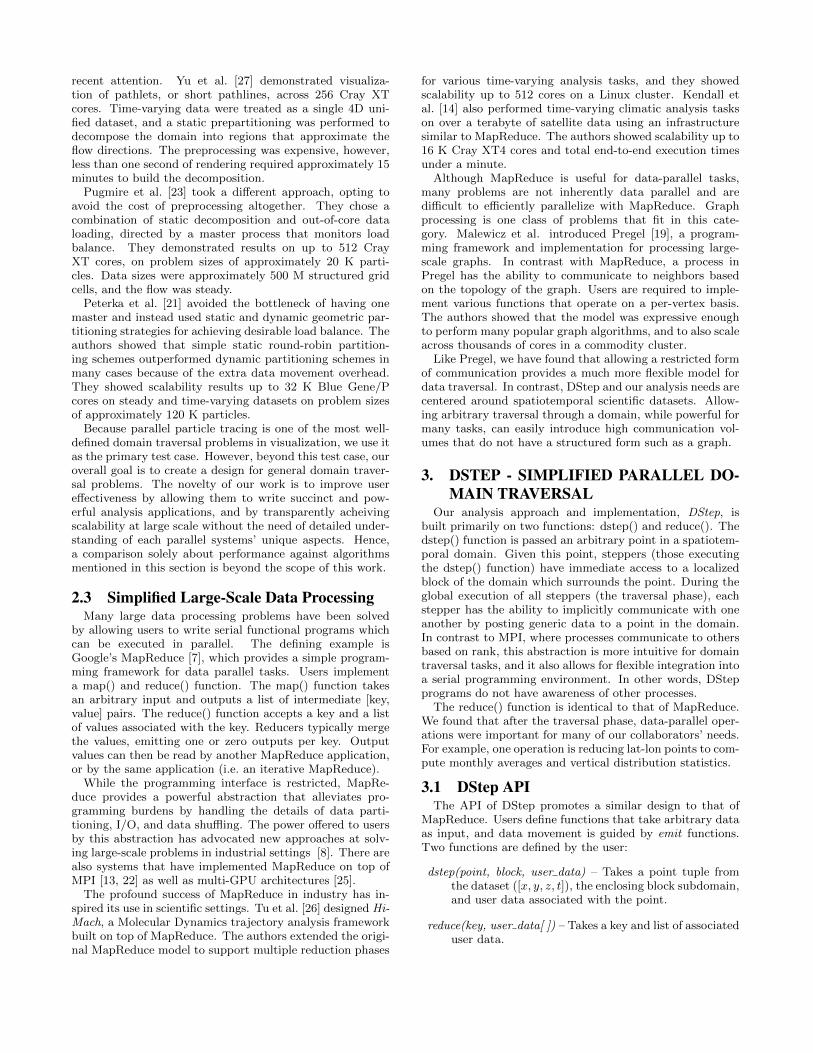
Figure 3: The software design of DStep is shown,with open-source modules in gray and custom com-ponents in other colors.

4. THE DSTEP RUNTIMEThe DStep Runtime is a C++ hybrid threaded/MPI exe-

cution system that is designed to perform complex domaintraversal tasks on large scientific datasets directly after sim-ulation. In contrast with industrial scenarios that leveragelarge commodity clusters for batch jobs [7], we designed ourimplementation to leverage HPC architectures for scientificanalysis scenarios.

4.1 Software ArchitectureA general overview of the DStep software stack is illus-

trated in Figure 3. Components are shown in a bottom-upfashion with open-source tools in gray and our componentsin other colors.

DStep utilizes up to four different types of workers perMPI process: steppers, reducers, communicators, and writ-ers. The Worker Superclass specifies three virtual functionsfor work scheduling, which manage the inherited incomingand outgoing work buffers. This management is describedin detail in the next subsection. The general responsibilitiesof the workers are as follows.

Stepper – Steppers own one or more blocks from a staticround-robin distribution of the domain. They are re-sponsible for reading the blocks, processing the user’squery on each block, sending the queried input todstep(), and sending any input from other steppersto dstep().

Reducer – Reducers own a map of keys that have an associ-ated array of values. They are responsible for sendingthis input to reduce() when the traversal phase hasfinished.

Communicator – As we will describe later, communicationhappens in a group-based manner. The sole responsi-bility of communicators is to act as masters of a workergroup, managing worker/application state and routingany long-range messages to other groups.

Writer – Writers manage data sent to the emit write()function and use a fixed functionality for data output.We note that we also provide the user to override awrite() function for sending output to other channelssuch as sockets.

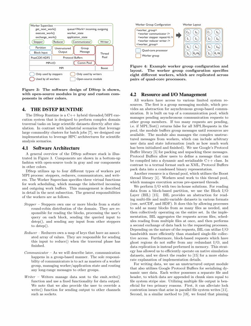
Worker Group Configuration

<worker_group> <worker communicator /> <worker stepper repeat=6 /> <worker reducer writer /></worker_group>

Worker Layout

C0 S0

S1 S2

S3 S4

S5 R0W0

C1 S6

S7 S8

S9 S10

S11 R1W1

Quad-core processor

Worker group

Figure 4: Example worker group configuration andlayout. The worker group configuration specifieseight different workers, which are replicated acrosspairs of quad-core processors.

4.2 Resource and I/O ManagementAll workers have access to various limited system re-

sources. The first is a group messaging module, which pro-vides an abstraction for asynchronous group-based commu-nication. It is built on top of a communication pool, whichmanages pending asynchronous communication requests toother group members. If too many requests are pending,i.e. if MPI Test() returns false for all MPI Requests in thepool, the module buffers group messages until resources areavailable. The module also manages the complex unstruc-tured messages from workers, which can include arbitraryuser data and state information (such as how much workhas been initialized and finished). We use Google’s ProtocolBuffer library [5] for packing and unpacking these messages.Protocol Buffers allow users to define a message that canbe compiled into a dynamic and serializable C++ class. Incontrast to a textual format such as XML, Protocol Bufferspack data into a condensed binary representation.

Another resource is a thread pool, which utilizes the Boostthread library [1]. Workers send work to this thread pool,which manages execution across pre-spawned threads.

We perform I/O with two in-house solutions. For readingdata from a block-based partition, we use the Block I/OLayer (BIL) [15]. BIL provides an abstraction for read-ing multi-file and multi-variable datasets in various formats(raw, netCDF, and HDF). It does this by allowing processesto add as many blocks from as many files as needed, andthen collectively operating on the entire set. In the imple-mentation, BIL aggregates the requests across files, sched-ules reading from multiple files at once, and then performsa second exchange of data back to the requesting processes.Depending on the nature of the requests, BIL can utilize I/Obandwidth more efficiently than standard single-file collec-tive access. Furthermore, block-based requests which haveghost regions do not suffer from any redundant I/O, anddata replication is instead performed in memory. This strat-egy has allowed us to efficiently operate on native simulationdatasets, and we direct the reader to [15] for a more elabo-rate explanation of implementation details.

For writing data, we use an unstructured output modulethat also utilizes Google Protocol Buffers for serializing dy-namic user data. Each writer possesses a separate file andheader, to which data are appended in chunk sizes equal tofile system stripe size. Utilizing multiple file output is ben-eficial for two primary reasons. First, it can alleviate lockcontention issues that arise in parallel file system writes [11].Second, in a similar method to [18], we found that pinning

In

Out

In

Out

In

Out

In

Out

In

Out

In

Out

In

Out

In

Out

In

Out

S0

S1

C0

S0

S1

C0

S0

S1

C0

In

Out

In

Out

In

Out

In

Out

In

Out

In

Out

In

Out

In

Out

In

Out

S0

S1

C0

S0

S1

C0

S0

S1

C0

In

Out

In

Out

In

Out

In

Out

In

Out

In

Out

In

Out

In

Out

In

Out

C1

S2

S3

C1

S2

S3

C1

S2

S3

In

Out

In

Out

In

Out

In

Out

In

Out

In

Out

In

Out

In

Out

In

Out

C1

S2

S3

C1

S2

S3

C1

S2

S3

Work message

Work and worker state message

Work and application state message

Worker group

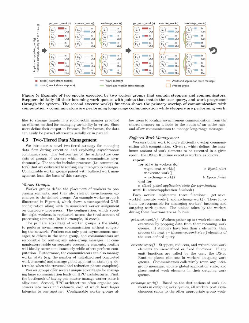
Figure 5: Example of two epochs executed by two worker groups that contain steppers and communicators.Steppers initially fill their incoming work queues with points that match the user query, and work progressesthrough the system. The second execute work() function shows the primary overlap of communication withcomputation - communicators are performing long-range communication while steppers are performing work.

files to storage targets in a round-robin manner providedan efficient method for managing variability in writes. Sinceusers define their output in Protocol Buffer format, the datacan easily be parsed afterwards serially or in parallel.

4.3 Two-Tiered Data ManagementWe introduce a novel two-tiered strategy for managing

data flow during execution and exploiting asynchronouscommunication. The bottom tier of the architecture con-sists of groups of workers which can communicate asyn-chronously. The top tier includes processes (i.e. communica-tors) that are dedicated to routing any inter-group messages.Configurable worker groups paired with buffered work man-agement form the basis of this strategy.

Worker Groups.Worker groups define the placement of workers to pro-

cessing elements, and they also restrict asynchronous ex-changes to the defined groups. An example worker group isillustrated in Figure 4, which shows a user-specified XMLconfiguration along with its associated worker assignmenton quad-core processors. The configuration, which speci-fies eight workers, is replicated across the total amount ofprocessing elements (in this example, 16 cores).

The primary advantage of worker groups is the abilityto perform asynchronous communication without congest-ing the network. Workers can only post asynchronous mes-sages to others in the same group, and communicators areresponsible for routing any inter-group messages. If com-municators reside on separate processing elements, routingwill ideally occur simultaneously while others perform com-putation. Furthermore, the communicators can also manageworker state (e.g. the number of initialized and completedwork elements) and manage global application state (e.g. de-termine when the traversal and reduction phases complete).

Worker groups offer several unique advantages for manag-ing large communication loads on HPC architectures. First,the bottleneck of having one master manage worker state isalleviated. Second, HPC architectures often organize pro-cessors into racks and cabinets, each of which have largerlatencies to one another. Configurable worker groups al-

low users to localize asynchronous communication, from theshared memory on a node to the nodes of an entire rack,and allow communicators to manage long-range messages.

Buffered Work Management.Workers buffer work to more efficiently overlap communi-

cation with computation. Given �, which defines the max-imum amount of work elements to be executed in a givenepoch, the DStep Runtime executes workers as follows:

repeatfor all w in workers do

w.get next work(�) � Epoch startw.execute work()w.exchange work() � Epoch finish

end for� Check global application state for termination

until Runtime::application finished()

Each worker implements three functions: get nextwork(�), execute work(), and exchange work(). These func-tions are responsible for managing workers’ incoming andoutgoing work queues. The actions taken by the workersduring these functions are as follows:

get next work(�) –Workers gather up to � work elements forexecution by popping data from their incoming workqueues. If steppers have less than � elements, theyprocess the next �− incoming work.size() elements ofthe user-defined query.

execute work() – Steppers, reducers, and writers pass workelements to user-defined or fixed functions. If anyemit functions are called by the user, the DStepRuntime places elements in workers’ outgoing workqueues. Communicators collectively route any inter-group messages, update global application state, andplace routed work elements in their outgoing workqueues.

exchange work() – Based on the destinations of work ele-ments in outgoing work queues, all workers post asyn-chronous sends to the other appropriate group work-

ers. If resources are not available, i.e. if the commu-nication pool has too many pending requests, workerssimply retain work in their outgoing work queues. Ifany worker has new state information, it is posted tothe communicator of the group. Similarly, if the com-municator has new application state information, it isposted to all of the group workers. After sends areposted, workers poll and add any incoming messagesto their incoming work queue.

Execution is designed such that workers sufficiently over-lap communication and computation without overloadingthe network. Furthermore, � is chosen to be sufficiently large(≈250) such that enough computation occurs while incom-ing asynchronous messages are buffered by the network.

We provide a thorough example of two epochs of execu-tion in Figure 5. For simplicity, we only use two groupswith communicators and steppers, and we show executionof functions in a synchronous manner. We note, however,that synchronization only happens among communicatorsduring execute work().

The user starts by executing their application with theDStep environment and providing a query as input. In thefirst epoch, steppers’ incoming work queues are filled with� query results. The incoming work is then sent to dstep(),which calls emit dstep() for each element in this example.Work elements are placed in steppers’ outgoing work queuesand then exchanged. In the example, S0 and S2 both havework elements that need to be sent to steppers outside thegroup (which is posted to their respective communicators)and inside the group (which is posted directly to them).

In the second epoch, querying happens in the same man-ner, with S1 and S3 appending queried elements to queuesthat already include incoming work from others. Steppersperform execution similar to the previous epoch, and com-municators exchange work and update the application state.Exchange occurs similar to the previous epoch, except com-municators now post any new application state informationand inter-group work messages from the previous epoch.

The entire traversal phase completes when the number ofinitialized dstep() tasks equal the number completed. Thereducers, although not illustrated in our example, wouldthen be able to execute work elements that were added totheir incoming work queues from emit reduce() calls. In arelated fashion to steppers, reducers also maintain state in-formation since they have the ability to proceed throughmultiple reduction phases.

In contrast to the synchronous particle tracing strategypresented in [21] and the strategy that used a single masterin [23], we have found this hybrid and highly asynchronousstrategy to be beneficial to our data demands. We demon-strate the performance of the DStep Runtime in the contextof our driving application – terascale atmospheric analysis.

5. DRIVING APPLICATION RESULTSOur initial user need was the ability to analyze telecon-

nections and perform internal-model variability studies. Ateleconnection can generally be described as a significantpositive or negative correlation in the fluctuations of a fieldat widely separated points. We provide an overview of ourdataset, the technical use case of our analysis problem, andthen driving results in inter-hemisphere exchange. We thenprovide a performance evaluation of our application.

March 2000

January 2000

SourceDestination

Densely seed source area

Advect particles through time

Quantitatively analyze destination during advection

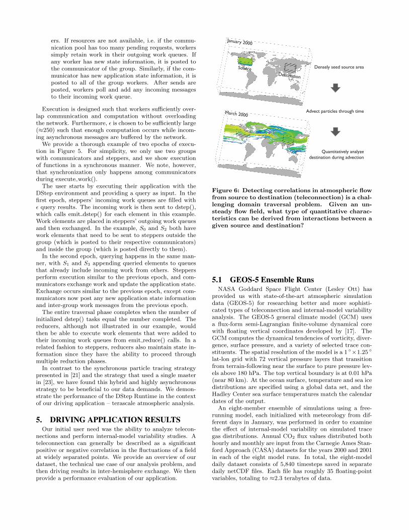
Figure 6: Detecting correlations in atmospheric flowfrom source to destination (teleconnection) is a chal-lenging domain traversal problem. Given an un-steady flow field, what type of quantitative charac-teristics can be derived from interactions between agiven source and destination?

5.1 GEOS-5 Ensemble RunsNASA Goddard Space Flight Center (Lesley Ott) has

provided us with state-of-the-art atmospheric simulationdata (GEOS-5) for researching better and more sophisti-cated types of teleconnection and internal-model variabilityanalysis. The GEOS-5 general climate model (GCM) usesa flux-form semi-Lagrangian finite-volume dynamical corewith floating vertical coordinates developed by [17]. TheGCM computes the dynamical tendencies of vorticity, diver-gence, surface pressure, and a variety of selected trace con-stituents. The spatial resolution of the model is a 1 ◦×1.25 ◦

lat-lon grid with 72 vertical pressure layers that transitionfrom terrain-following near the surface to pure pressure lev-els above 180 hPa. The top vertical boundary is at 0.01 hPa(near 80 km). At the ocean surface, temperature and sea icedistributions are specified using a global data set, and theHadley Center sea surface temperatures match the calendardates of the output.

An eight-member ensemble of simulations using a free-running model, each initialized with meteorology from dif-ferent days in January, was performed in order to examinethe effect of internal-model variability on simulated tracegas distributions. Annual CO2 flux values distributed bothhourly and monthly are input from the Carnegie Ames Stan-ford Approach (CASA) datasets for the years 2000 and 2001in each of the eight model runs. In total, the eight-modeldaily dataset consists of 5,840 timesteps saved in separatedaily netCDF files. Each file has roughly 35 floating-pointvariables, totaling to ≈2.3 terabytes of data.

Average CO fossil fuel until arrival (ppm)2Time until arrival (days)

0 30 60 0 0.000183 0.000367

January

July

Ensemble 1 Ensemble 2 Ensemble 1 Ensemble 2

January

July

A

B

C

D

Figure 7: Three-dimensional direct volume renderings of the time until arrival and average CO2 concentrationsfrom January and July in two GEOS-5 ensemble runs. The circled areas are explained in Section 5.3.

5.2 Technical Use CaseThe technical requirements of our studies involved quan-

titatively assessing relationships among the flows from dif-ferent sources to different destinations. Figure 6 illustratesthe general problem and approach. Given an unsteady flowfield and an initial source of flow (the United States), howcan we assess the relationships of the flow with respect to adestination area (China in this example)? While a visualiza-tion method such as fieldline rendering can be used (such asin this example), it is difficult for the user to quantitativelyassess the relationship. For example, our collaborators wereinterested in the following analyses:

Time Until Arrival – Starting from the source at variouspoints in time, how long does it take for the flow fieldto reach the destination?

Residence Time – Once the flow enters the destination, howlong does it reside in the area before exiting?

Average CO2 Until Arrival – What is the concentration ofvarious CO2 properties along the path to the destina-tion area?

Internal-Model Variability – Given these quantitative anal-yses, how can they be used in a manner for assessingvariability of models with different initial conditions?

Along with these initial challenges, another need from ourusers was the ability to operate in four dimensions. TheGEOS-5 dataset has a time-varying hybrid-sigma pressuregrid, with units in meters per second in the horizontal layersand Pascals per second in the vertical direction. Dealingwith this grid in physical space involves adjusting for thecurvilinear structure of the lat-lon grid and then utilizinganother variable in the dataset to determine the pressurethickness at each voxel. Our collaborators were unawareof any tools that could process the flow of their grid usingall four dimensions, and we wrote a custom Runge-Kuttaintegration kernel for this purpose.

The dstep() function of our application is similar to theexample from Section 3, with the exception that particlescarry statistics during integration. After each Runge-Kuttastep, the particles perform the following function:

function update particle(particle)if particle.in destination() then

if particle.has already arrived() thenparticle.residence time += StepSize

elseparticle.time until arrival = particle.timeparticle.residence time = 0

end ifelse

particle.co2 accumulation += particle.co2end if

end function

The particles are then reduced based on their starting gridpoint and the month from which they began tracing. Thereduce function then performs point-wise operations of thedaily data, averaging it into monthly values. The reduce()function operates in the following manner:

function reduce(key, particles[ ])Result model results[NumModels]for all p in particles[ ] do

� Compute monthly averages for each modelmodel results[p.model].update stats(p)

end forfor all r in model results[ ] do

emit write(r) � Store statisticsend for

end function

Once finished, the computed statistics may then be ren-dered and compared with standard point-based techniques.

5.3 Application Impact – Studying Inter-Hemisphere Exchange

We used the previously described application to analyzethe effects of the flow field from lower levels of the NorthernHemisphere to the lower levels of the Southern Hemisphere.The interaction of the two areas is important since the dis-tributions of heat, moisture, CO2 and other chemical tracersare critically dependent on exchange between the Northernand Southern Hemispheres. We first used DStep to queryfor the lower 22 pressure layers of the Northern Hemisphere,and particle tracers were initialized from each queried point.The destination location was set to the lower 22 pressurelayers of the Southern Hemisphere.

Since our dataset has a relatively short time span (twoyears), we focused on small-scale interactions. Specifically,we only saved particles which reached the destination areain under two months. Particles were emitted in five day timeintervals for the first year of each model, and each particlewas allowed to travel for a year. Before hitting the desti-nation area, particles accumulated CO2 information at eventime samplings and used this to compute the average con-centrations along the trace. Once hitting the target destina-tion, particles then accumulated residence time informationuntil exiting the area. If particles exited the area or did notreach it within two months, they were terminated.

We gathered interesting observations using the time un-til arrival and CO2 concentrations. Three-dimensional ren-derings of these characteristics from January and July intwo of the ensemble runs are shown in Figure 7. The timeuntil arrival starting from January shows interesting prop-erties right along the border of the hemispheres. BetweenSouth America and Africa (circle A), one can observe a gapwhere the particles take up to two months to reach theSouthern Hemisphere. In contrast to the surrounding ar-eas, where particles almost immediately reach the SouthernHemisphere, this area is a likely indicator of exchange. Ex-amining the CO2 concentration at this gap (circle D), onecan also observe that the particles traveled through areaswith much higher CO2 concentration.

Time until arrival also shows interesting characteristics inJuly. In the summer months, the jet stream is located closerto border of the United States and Canada. It appears tobe directing many of the particles eastward, which then gointo an area of strong downward flow. This downward flowis more apparent in the second ensemble (circle C), resem-bling the shape of a walking cane. The scientists believedthis area could potentially be responsible for much of the in-teraction that is occurring between the area around the jetstream and the Southern Hemisphere. When observing theCO2 July rendering, one can observe that many of the mainCO2 emitters potentially carry more CO2 into the SouthernHemisphere.

One can also arrive at conclusions from visually compar-ing the ensembles. For example, a structure appears overCanada in January of ensemble two (circle B), but not inensemble one. For a closer look, we computed the probabil-ity that a given lat-lon point over all of the queried verti-cal layers made it to the Southern Hemisphere within twomonths. We plotted the absolute differences in probabilityin Figure 8. Color represents the model which had higherprobability, and the opacity of color is modulated by theabsolute difference to highlight differences between the en-sembles. One can observe that in January near the Hawai-

January July

Ensemble 1 Ensemble 2

Figure 8: Differences between two ensemble runsare revealed by examining their probability distri-butions in the vertical direction. Color indicates theensemble that had a higher probability of flow trav-eling from the Northern to Southern Hemispherewithin two months. The opacity of this color is mod-ulated by the absolute difference between the twoensembles, revealing the areas that are different.

ian area of the Pacific Ocean, particles have a much higherprobability of reaching the Southern Hemisphere in ensem-ble one. As mentioned before, one can also see the structurefrom ensemble two appearing over Canada in January. InJuly, the models appear to have similar probabilistic char-acteristics, which could potentially mean that the ensemblesare converging through time.

5.4 Performance EvaluationWe have evaluated performance of the DStep Runtime in

the context of our driving application. Our testing environ-ment is Intrepid, an IBM BlueGene/P supercomputer at Ar-gonne National Laboratory. Intrepid contains 40,960 nodes,each containing four cores. We used virtual node mode onIntrepid, which treats each core as a separate process. Wealso used Intrepid’s General Parallel File System (GPFS) forstorage and I/O performance results.

We used five variables in the GEOS-5 application. Threevariables are horizontal wind and vertical pressure velocities.One variable provides the vertical grid warping, and the lastvariable is the CO2 fossil fuel concentration. The dataset isstored in its original netCDF format across 5,840 files. Thefive variables total to approximately 410 GB.

For inter-hemisphere analysis, the application issued aquery for the lower 22 vertical layers of the Northern Hemi-sphere. We strided the queried results by a factor of two ineach spatial dimension and performed this query for the firstyear of each of the eight ensemble runs in five day intervals.The application initialized approximately 40 million queriedparticles, which could be integrated up to a year before ter-mination. Many of the particles, however, would be cut offafter two months of integration if they had not yet arrivedin the Southern Hemisphere.

The tests utilized a worker group of 16 workers that con-sisted of 15 steppers on separate cores. Reducers, writers,and communicators were placed on the 16th core of eachgroup. Although reducers and writers could potentially in-terfere with the routing performance of the communicators,this application had small reduction and data output re-quirements. In total, approximately 400 MB of informationwere written by the application.

Each worker was configured to own two blocks from thedomain and could use up to 128 MB of memory. Becauseof the memory restrictions, models were processed one at

10

100

1,000

10,000

1 K 2 K 4 K 8 K 16 K 32 K 64 K

Tim

e (

seconds)

Processes

Total Time

Total Time

Instantiation

Optimal Scaling1,870

165

(a) Total Time (log-log scale)

100

1,000

10,000

1 K 2 K 4 K 8 K 16 K 32 K 64 K

0

0.2

0.4

0.6

0.8

1

Bandw

idth

(M

B/s

)

Percenta

ge o

f IO

R

Processes

Read Bandwidth

Bandwidth

Percent of IOR

(b) Read Bandwidth (log-log scale)

45

50

55

60

65

70

75

80

85

90

1 K 2 K 4 K 8 K 16 K 32 K 64 K

Byte

s (G

B)

Processes

Total Bytes Communicated

(c) Bytes Communicated

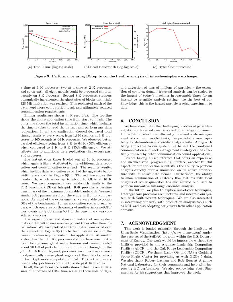
Figure 9: Performance using DStep to conduct entire analysis of inter-hemisphere exchange.

a time at 1 K processes, two at a time at 2 K processes,and so on until all eight models could be processed simulta-neously on 8 K processes. Beyond 8 K processes, steppersdynamically incremented the ghost sizes of blocks until their128 MB limitation was reached. This replicated much of thedata, kept more computation local, and ultimately reducedcommunication requirements.

Timing results are shown in Figure 9(a). The top lineshows the entire application time from start to finish. Theother line shows the total instantiation time, which includesthe time it takes to read the dataset and perform any datareplication. In all, the application showed decreased totaltiming results at every scale, from 1,870 seconds at 1 K pro-cesses to 165 seconds at 64 K processes. We observed betterparallel efficiency going from 8 K to 64 K (50% efficiency)when compared to 1 K to 8 K (35% efficiency). We at-tribute this to additional data replication that occurs past8 K processes.

The instantiation times leveled out at 16 K processes,which again is likely attributed to the additional data repli-cation and communication overhead. The reading results,which include data replication as part of the aggregate band-width, are shown in Figure 9(b). The red line shows thebandwidth, which scales up to about 10 GB/s at 16 Kcores. We have compared these bandwidth results to theIOR benchmark [3] on Intrepid. IOR provides a baselinebenchmark of the maximum obtainable bandwidth. We usedsimilar IOR parameters from the study in [16] for compar-isons. For most of the experiements, we were able to obtain50% of the benchmark. For an application scenario such asours, which operates on thousands of multivariable netCDFfiles, consistently obtaining 50% of the benchmark was con-sidered a success.

The asynchronous and dynamic nature of our systemmakes it difficult to measure component times other than ini-tialization. We have plotted the total bytes transferred overthe network in Figure 9(c) to better illustrate some of thecommunication requirements of this application. At smallerscales (less than 16 K), processes did not have much extraroom for dynamic ghost size extension and communicatedabout 90 GB of particle information in total throughout thejob. At 16 K and beyond, processes have much more roomto dynamically resize ghost regions of their blocks, whichin turn kept more computation local. This is the primaryreason why job times continue to scale past 16 K cores.

In all, the performance results showed that – even at datasizes of hundreds of GBs, time scales at thousands of days,

and advection of tens of millions of particles – the execu-tion of complex domain traversal analysis can be scaled tothe largest of today’s machines in reasonable times for aninteractive scientific analysis setting. To the best of ourknowledge, this is the largest particle tracing experiment todate.

6. CONCLUSIONWe have shown that the challenging problem of paralleliz-

ing domain traversal can be solved in an elegant manner.Our solution, which can efficiently hide and scale manage-ment of complex parallel tasks, has provided a new capa-bility for data-intensive scientific analysis tasks. Along withbeing applicable to our system, we believe the two-tieredcommunication and work management strategy can be effec-tively utilized by other communication-bound applications.

Besides having a user interface that offers an expressiveand succinct serial programming interface, another fruitfulaspect for our application scientists is the ability to performanalysis directly after a simulation on its native architec-ture with its native data format. Furthermore, the abilityto allow combination of unsteady flow features with localanalysis of scalar quantities has also allowed our users toperform innovative full-range ensemble analysis.

In the future, we plan to explore out-of-core techniques,heterogeneous processor architectures, and integrate our sys-tem with fault-tolerant techniques. We are also interestedin integrating our work with production analysis tools suchas NCL and also adopting early users from other applicationdomains.

7. ACKNOWLEDGMENTThis work is funded primarily through the Institute of

Ultra-Scale Visualization (http://www.ultravis.org) underthe auspices of the SciDAC program within the U.S. Depart-ment of Energy. Our work would be impossible without thefacilities provided by the Argonne Leadership ComputingFacility (ALCF) and the Oak Ridge Leadership ComputingFacility (OLCF). We thank Lesley Ott and NASA GoddardSpace Flight Center for providing us with GEOS-5 data.We also thank Robert Latham and Rob Ross at ArgonneNational Laboratory for their comments and help with im-proving I/O performance. We also acknowledge Scott Sim-merman for his suggestions that improved the work.

8. REFERENCES[1] Boost C++ libraries. http://www.boost.org.[2] IDL: Interactive data language.

http://www.ittvis.com/idl.[3] IOR benchmark.

http://www.cs.sandia.gov/Scalable_IO/ior.html.[4] NCL: NCAR command language.

http://www.ncl.ucar.edu.[5] Protocol Buffers: Google’s data interchange format.

http://code.google.com/p/protobuf.[6] Visit: Software that delivers parallel interactive

visualization. https://wci.llnl.gov/codes/visit.[7] Jeffrey Dean and Sanjay Ghemawat. Mapreduce:

Simplified data processing on large clusters. In OSDI‘04: Sixth Symposium on Operating System Designand Implementation, 2004.

[8] Jeffrey Dean and Sanjay Ghemawat. Mapreduce:Simplified data processing on large clusters.Communications of the ACM, 51:107–113, January2008.

[9] D. J. Erickson, R. T. Mills, J. Gregg, T. J. Blasing,F. M. Hoffman, R.J. Andres, M. Devries, Z. Zhu, andS. R. Kawa. An estimate of monthly global emissionsof anthropogenic CO2: The impact on the seasonalcycle of atmospheric CO2. Journal of GeophysicalResearch, 113, 2007.

[10] D. Galbally, K. Fidkowski, K. Willcox, andO. Ghattas. Non-linear model reduction foruncertainty quantification in large-scale inverseproblems. International Journal for NumericalMethods in Engineering, 81(12):1581–1608, 2010.

[11] Kui Gao, Wei keng Liao, Arifa Nisar, Alok Choudhary,Robert Ross, and Robert Latham. Using subfiling toimprove programming flexibility and performance ofparallel shared-file i/o. International Conference onParallel Processing, pages 470–477, 2009.

[12] A. Hannachi, I. T. Jolliffe, and D.B. Stephenson.Empirical orthoghonal functions and relatedtechniques in atmospheric science: A review.International Journal of Climatology, 27:1119–1152,2007.

[13] T. Hoefler, A. Lumsdaine, and J. Dongarra. Towardsefficient mapreduce using MPI. In Recent Advances inParallel Virtual Machine and Message PassingInterface, 16th European PVM/MPI Users’ GroupMeeting. Springer, Sep. 2009.

[14] Wesley Kendall, Markus Glatter, Jian Huang, TomPeterka, Robert Latham, and Robert Ross. Terascaledata organization for discovering multivariate climatictrends. In SC ‘09: Proceedings of ACM/IEEESupercomputing 2009, Nov. 2009.

[15] Wesley Kendall, Jian Huang, Tom Peterka, RobLatham, and Robert Ross. Visualization viewpoint:Towards a general I/O layer for parallel visualizationapplications. IEEE Computer Graphics andApplications, 31(6), Nov./Dec. 2011.

[16] Samuel Lang, Philip Carns, Robert Latham, RobertRoss, Kevin Harms, and William Allcock. I/Operformance challenges at leadership scale. In SC ‘09:Proceedings of ACM/IEEE Supercomputing 2009,2009.

[17] S-J Lin. A “vertically lagrangian” finite-volume

dynamical core for global models. Monthly WeatherReview, 132:2293–2307.

[18] Jay Lofstead, Fang Zheng, Qing Liu, Scott Klasky,Ron Oldfield, Todd Kordenbrock, Karsten Schwan,and Matthew Wolf. Managing variability in the I/Operformance of petascale storage systems. In SC ‘10:Proceedings of ACM/IEEE Supercomputing 2010,2010.

[19] Grzegorz Malewicz, Matthew H. Austern, Aart J.CBik, James C. Dehnert, Ilan Horn, Naty Leiser, andGrzegorz Czajkowski. Pregel: A system for large-scalegraph processing. In Proceedings of the 2010International Conference on Management of Data,SIGMOD ’10, pages 135–146, 2010.

[20] L. Ott, B. Duncan, S. Pawson, P. Colarco, M. Chin,C. Randles, T. Diehl, and E. Nielsen. Influence of the2006 Indonesian biomass burning aerosols on tropicaldynamics studied with the GEOS-5 AGCM. Journalof Geophysical Research, 115, 2010.

[21] Tom Peterka, Robert Ross, B. Nouanesengsey,Teng-Yok Lee, Han-Wei Shen, Wesley Kendall, andJian Huang. A study of parallel particle tracing forsteady-state and time-varying flow fields. In IEEEInternational Parallel and Distributed ProcessingSymposium (IPDPS), May 2011.

[22] Steven J. Plimpton and Karen D. Devine. Mapreducein mpi for large-scale graph algorithms. 2011.

[23] Dave Pugmire, Hank Childs, Christoph Garth, SeanAhern, and Gunther H. Weber. Scalable computationof streamlines on very large datasets. In Proceedings ofthe 2009 ACM/IEEE conference on Supercomputing,2009.

[24] Kurt Stockinger, John Shalf, Kesheng Wu, and E. WesBethel. Query-Driven Visualization of Large DataSets. In Proceedings of IEEE Visualization 2005, pages167–174. IEEE Computer Society Press, October2005. LBNL-57511.

[25] Jeff Stuart and John Owens. Multi-GPU MapReduceon GPU clusters. In IEEE International Parallel andDistributed Processing Symposium (IPDPS), May2011.

[26] Tiankai Tu, Charles A. Rendleman, David W.Borhani, Ron O. Dror, Justin Gullingsrud, Morten Ø.Jensen, John L. Klepeis, Paul Maragakis, PatrickMiller, Kate A. Stafford, and David E. Shaw. Ascalable parallel framework for analyzing terascalemolecular dynamics simulation trajectories. InProceedings of the 2008 ACM/IEEE conference onSupercomputing, SC ’08, 2008.

[27] Hongfeng Yu, Chaoli Wang, and Kwan-Liu Ma.Parallel hierarchical visualization of large time-varying3d vector fields. In Proceedings of the 2007ACM/IEEE conference on Supercomputing, SC ’07,pages 1–24, 2007.