Alexander Litvinenko, Quanti cation Center, KAUST · PDF fileFast and cheap approximation of...

Fast and cheap approximation of large covariancematrices by the hierarchical matrix technique

Alexander Litvinenko,Extreme Computing Research Center and Uncertainty

Quantification Center, KAUST(joint work with M. Genton, Y. Sun and D. Keyes)

Center for UncertaintyQuantification


Center for Uncertainty Quantification Logo Lock-up

http://sri-uq.kaust.edu.sa/

http://sri-uq.kaust.edu.sa/

4*

The structure of the talk

1. Hierarchical matrices [Hackbusch 1999]: Low-rank matrices,cluster tree, block cluster tree and admissibility condition, costand storage, (www.hlib.org)

2. Matern covariance function

3. Uncertain parameters of the covariance function:

3.1 Uncertain covariance length3.2 Uncertain smoothness parameter

4. Identification of these parameters via maximizing thelog-likelihood.




2 / 54

4*

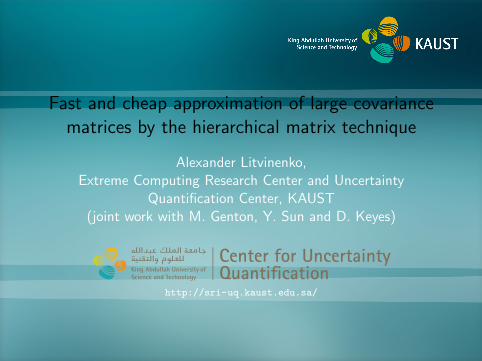
Motivation for H-matrices

Ax = b

Iterative methods: Jacobi, Gauss- Seidel, SOR, ...Complexity O(#iters · n) or O(#iters · n2), number of iteration isproportional to

√cond(A).

Direct solvers: Gaussian elimination, domain decompositions, LU,...Cost of A−1 is O(n3)

If A is structured (diagonal, Toeplitz, circulant) then can apply e.g.FFT with O(nlogn), but if not ?What if you need not only x = A−1b, but f (A)(e.g. A−1, expA, sinA, signA, ...)?




3 / 54

4*

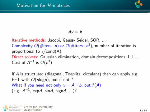
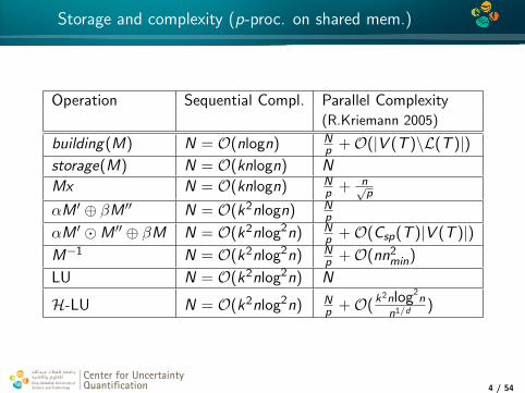
Storage and complexity (p-proc. on shared mem.)

Operation Sequential Compl. Parallel Complexity(R.Kriemann 2005)

building(M) N = O(nlogn) Np +O(|V (T )\L(T )|)

storage(M) N = O(knlogn) N

Mx N = O(knlogn) Np + n√

p

αM ′ ⊕ βM ′′ N = O(k2nlogn) Np

αM ′ M ′′ ⊕ βM N = O(k2nlog2n) Np +O(Csp(T )|V (T )|)

M−1 N = O(k2nlog2n) Np +O(nn2

min)

LU N = O(k2nlog2n) N

H-LU N = O(k2nlog2n) Np +O(k

2nlog2n

n1/d )




4 / 54

4*

Matern function for different parameters

[Whittle’63, D. Simpson, Finn Lindgren, Havard Rue, D. Bolin,...]

−2 −1.5 −1 −0.5 0 0.5 1 1.5 20

0.05

0.1

0.15

0.2

0.25

Matern covariance (nu=1)

σ=0.5, l=0.5

σ=0.5, l=0.3

σ=0.5, l=0.2

σ=0.5, l=0.1

−2 −1.5 −1 −0.5 0 0.5 1 1.5 20

0.05

0.1

0.15

0.2

0.25

nu=0.15

nu=0.3

nu=0.5

nu=1

nu=2

nu=30




5 / 54

4*

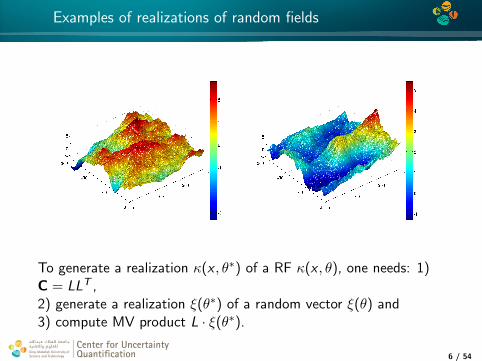
Examples of realizations of random fields

To generate a realization κ(x , θ∗) of a RF κ(x , θ), one needs: 1)C = LLT ,2) generate a realization ξ(θ∗) of a random vector ξ(θ) and3) compute MV product L · ξ(θ∗).




6 / 54

4*

Hierarchical (H)-matrices

Introduction into Hierarchical (H)-matrix technique




7 / 54

4*

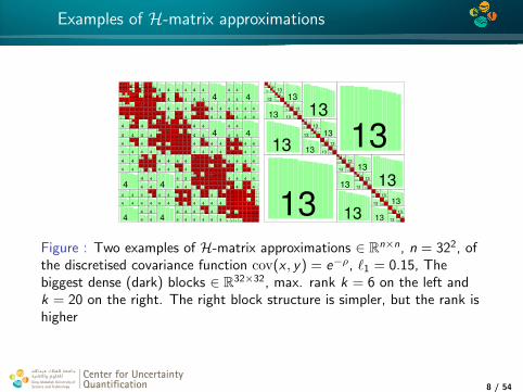
Examples of H-matrix approximations

25 20

20 20

20 16

20 16

20 20

16 16

20 16

16 16

4 4

20 4 32

4 4

16 4 32

4 20

4 4

4 16

4 4

32 32

20 20

20 20 32

32 32

4 3

4 4 32

20 4

16 4 32

32 4

32 32

4 32

32 32

32 4

32 32

4 4

4 4

20 16

4 4

32 32

4 32

32 32

32 32

4 32

32 32

4 32

20 20

20 20 32

32 32

32 32

32 32

32 32

32 32

32 32

32 32

4 44 4

20 4 32

32 32 4

4 4

32 4

32 32 4

4 4

32 32

4 32 4

4 4

32 32

32 32 4

4

4 20

4 4 32

32 32

4 4

432 4

32 32

4 4

432 32

4 32

4 4

432 32

32 32

4 4

20 20

20 20 32

32 32

4 4

20 4 32

32 32

4 20

4 4 32

32 32

20 20

20 20 32

32 32

32 4

32 32

32 4

32 32

32 4

32 32

32 4

32 32

32 32

4 32

32 32

4 32

32 32

4 32

32 32

4 32

32 32

32 32

32 32

32 32

32 32

32 32

32 32

32 32

4 4

4 4 44 4

20 4 32

32 32

32 4

32 32

4 32

32 32

32 4

32 32

4 4

4 4

4 4

4 4 4

4 4

32 4

32 32 4

4 4

4 4

4 4

4 4 4

432 4

32 32

4 4

4 4

4 4

4 4

4 4 432 4

32 32

32 4

32 32

32 4

32 32

32 4

32 32

4 4

4 4

4 4

4 4

4 20

4 4 32

32 32

4 32

32 32

32 32

4 32

32 32

4 32

44 4

4 4

4 4

4 4

4 4

32 32

4 32 4

44 3

4 4

4 4

4 4

432 32

4 32

4 4

44 4

4 4

4 4

4 4

32 32

4 32

32 32

4 32

32 32

4 32

32 32

4 32

44 4

4 4

20 20

20 20 32

32 32

32 32

32 32

32 32

32 32

32 32

32 32

4 4

20 4 32

32 32

32 4

32 32

4 32

32 32

32 4

32 32

4 20

4 4 32

32 32

4 32

32 32

32 32

4 32

32 32

4 32

20 20

20 20 32

32 32

32 32

32 32

32 32

32 32

32 32

32 32

4 4

32 32

32 32 4

4 4

32 4

32 32 4

4 4

32 32

4 32 4

4 4

32 32

32 32 4

432 32

32 32

4 4

432 4

32 32

4 4

432 32

4 32

4 4

432 32

32 32

4 4

32 32

32 32

32 32

32 32

32 32

32 32

32 32

32 32

32 4

32 32

32 4

32 4

32 4

32 32

32 4

32 4

32 32

4 32

32 32

4 32

32 32

4 4

32 32

4 4

32 32

32 32

32 32

32 32

32 32

32 32

32 32

32 32

25 11

11 20 12

1320 11

9 1613

13

20 11

11 20 13

13 3213

13

20 8

10 20 13

13 32 13

1332 13

13 32

13

13

20 11

11 20 13

13 32 13

13

20 10

10 20 12

12 3213

13

32 13

13 32 13

1332 13

13 32

13

13

20 11

11 20 13

13 32 13

1332 13

13 3213

13

20 9

9 20 13

13 32 13

1332 13

13 32

13

13

32 13

13 32 13

1332 13

13 3213

13

32 13

13 32 13

1332 13

13 32

Figure : Two examples of H-matrix approximations ∈ Rn×n, n = 322, ofthe discretised covariance function cov(x , y) = e−ρ, `1 = 0.15, Thebiggest dense (dark) blocks ∈ R32×32, max. rank k = 6 on the left andk = 20 on the right. The right block structure is simpler, but the rank ishigher




8 / 54

4*

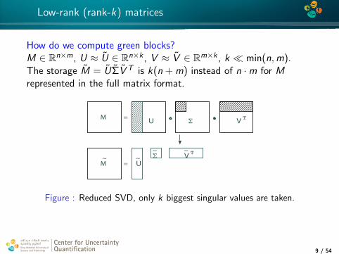
Low-rank (rank-k) matrices

How do we compute green blocks?M ∈ Rn×m, U ≈ U ∈ Rn×k , V ≈ V ∈ Rm×k , k min(n,m).The storage M = UΣV T is k(n + m) instead of n ·m for Mrepresented in the full matrix format.

VU ΣT=M

UVΣ∼

∼ ∼ T

=M∼

Figure : Reduced SVD, only k biggest singular values are taken.




9 / 54

4*

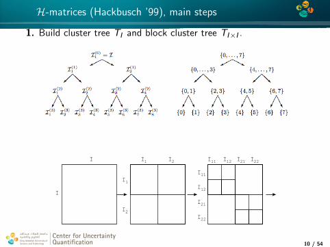
H-matrices (Hackbusch ’99), main steps

1. Build cluster tree TI and block cluster tree TI×I .

I

I

I I

I

I

I I I I1

1

2

2

11 12 21 22

I11

I12

I21

I22




10 / 54

4*

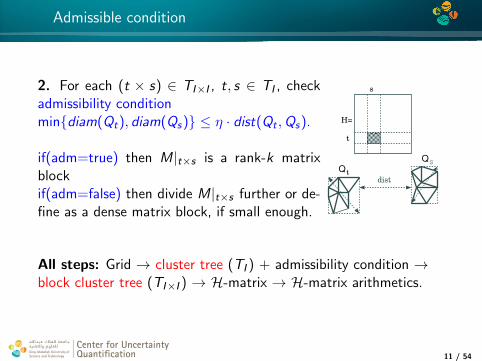
Admissible condition

2. For each (t × s) ∈ TI×I , t, s ∈ TI , checkadmissibility conditionmindiam(Qt), diam(Qs) ≤ η · dist(Qt ,Qs).

if(adm=true) then M|t×s is a rank-k matrixblockif(adm=false) then divide M|t×s further or de-fine as a dense matrix block, if small enough.

Q

Qt

S

dist

H=

t

s

All steps: Grid → cluster tree (TI ) + admissibility condition →block cluster tree (TI×I ) → H-matrix → H-matrix arithmetics.




11 / 54

4*

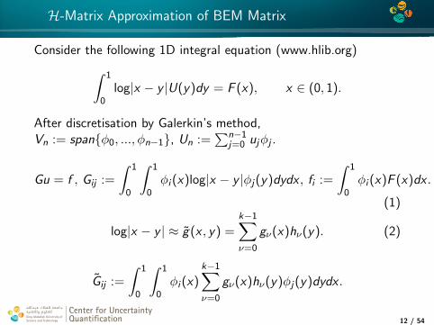
H-Matrix Approximation of BEM Matrix

Consider the following 1D integral equation (www.hlib.org)∫ 1

0log|x − y |U(y)dy = F (x), x ∈ (0, 1).

After discretisation by Galerkin’s method,Vn := spanφ0, ..., φn−1, Un :=

∑n−1j=0 ujφj .

Gu = f , Gij :=

∫ 1

0

∫ 1

0φi (x)log|x − y |φj(y)dydx , fi :=

∫ 1

0φi (x)F (x)dx .

(1)

log|x − y | ≈ g(x , y) =k−1∑ν=0

gν(x)hν(y). (2)

Gij :=

∫ 1

0

∫ 1

0φi (x)

k−1∑ν=0

gν(x)hν(y)φj(y)dydx .




12 / 54

4*

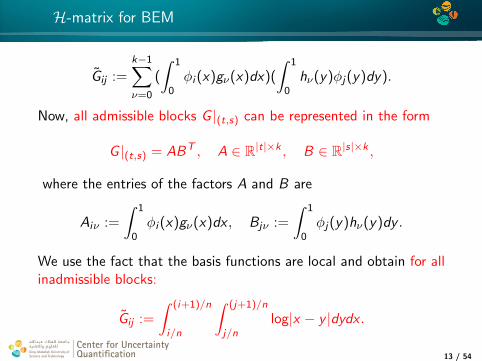
H-matrix for BEM

Gij :=k−1∑ν=0

(

∫ 1

0φi (x)gν(x)dx)(

∫ 1

0hν(y)φj(y)dy).

Now, all admissible blocks G |(t,s) can be represented in the form

G |(t,s) = ABT , A ∈ R|t|×k , B ∈ R|s|×k ,

where the entries of the factors A and B are

Aiν :=

∫ 1

0φi (x)gν(x)dx , Bjν :=

∫ 1

0φj(y)hν(y)dy .

We use the fact that the basis functions are local and obtain for allinadmissible blocks:

Gij :=

∫ (i+1)/n

i/n

∫ (j+1)/n

j/nlog|x − y |dydx .




13 / 54

4*

Numerical experiments with H-matrices

Computing time, storage of an H-matrixapproximation of a covariance matrix




14 / 54

4*

H - Matrices, storage and computing time

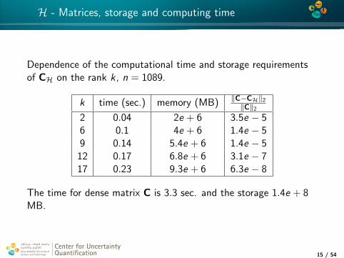
Dependence of the computational time and storage requirementsof CH on the rank k , n = 1089.

k time (sec.) memory (MB) ‖C−CH‖2

‖C‖2

2 0.04 2e + 6 3.5e − 56 0.1 4e + 6 1.4e − 59 0.14 5.4e + 6 1.4e − 5

12 0.17 6.8e + 6 3.1e − 717 0.23 9.3e + 6 6.3e − 8

The time for dense matrix C is 3.3 sec. and the storage 1.4e + 8MB.




15 / 54

4*

H - Matrices, dependence on cov. lengths

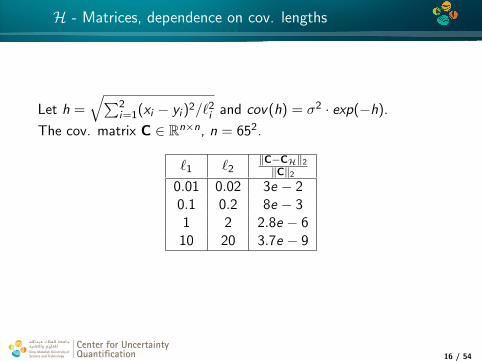
Let h =√∑2

i=1(xi − yi )2/`2i and cov(h) = σ2 · exp(−h).

The cov. matrix C ∈ Rn×n, n = 652.

`1 `2‖C−CH‖2

‖C‖2

0.01 0.02 3e − 20.1 0.2 8e − 31 2 2.8e − 6

10 20 3.7e − 9




16 / 54

4*

Memory and computational times

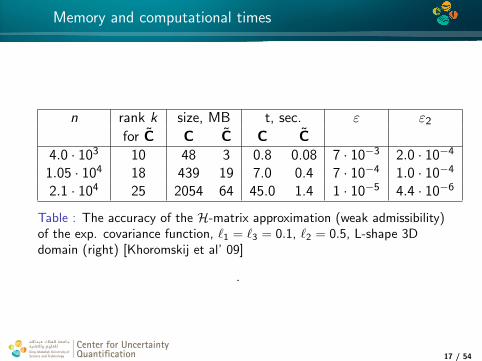
n rank k size, MB t, sec. ε ε2

for C C C C C4.0 · 103 10 48 3 0.8 0.08 7 · 10−3 2.0 · 10−4

1.05 · 104 18 439 19 7.0 0.4 7 · 10−4 1.0 · 10−4

2.1 · 104 25 2054 64 45.0 1.4 1 · 10−5 4.4 · 10−6

Table : The accuracy of the H-matrix approximation (weak admissibility)of the exp. covariance function, `1 = `3 = 0.1, `2 = 0.5, L-shape 3Ddomain (right) [Khoromskij et al’ 09]

.




17 / 54

4*

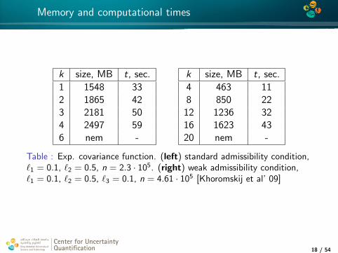
Memory and computational times

k size, MB t, sec.

1 1548 332 1865 423 2181 504 2497 596 nem -

k size, MB t, sec.

4 463 118 850 22

12 1236 3216 1623 4320 nem -

Table : Exp. covariance function. (left) standard admissibility condition,`1 = 0.1, `2 = 0.5, n = 2.3 · 105. (right) weak admissibility condition,`1 = 0.1, `2 = 0.5, `3 = 0.1, n = 4.61 · 105 [Khoromskij et al’ 09]




18 / 54

4*

Time and storage cost on the problem size n

time (sec.) memory (MB)

n C C C C ε

332 0.14 0.01 9.5 0.7 4.3 · 10−3

652 2.6 0.05 1.4 · 102 3.5 3.7 · 10−3

1292 −− 0.24 nem 16 −−2572 −− 1 nem 64 −−

Table : Dependence of the computational time and storage cost on theproblem size n, rank k = 5, cov(x , y) = e−ρ, `1 = `2 = 1, domainG = [0, 1]2.




19 / 54

4*

Identifying uncertain parameters

It was an additional materialLet us come to the main topic:Identifying uncertain parameters




20 / 54

4*

Identifying uncertain parameters

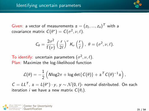
Given: a vector of measurements z = (z1, ..., zn)T with acovariance matrix C (θ∗) = C (σ2, ν, `).

Cθ =2σ2

Γ(ν)

( r

2`

)νKν

( r

`

), θ = (σ2, ν, `).

To identify: uncertain parameters (σ2, ν, `).Plan: Maximize the log-likelihood function

L(θ) = −1

2

(N log2π + log detC (θ)+ zTC (θ)−1z

),

C = LLT , z = L(θ∗) · y , y ∼ N (0, I )- normal distributed. On eachiteration i we have a new matrix C (θi ).




21 / 54

4*

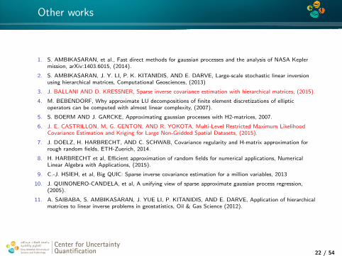
Other works

1. S. AMBIKASARAN, et al., Fast direct methods for gaussian processes and the analysis of NASA Keplermission, arXiv:1403.6015, (2014).

2. S. AMBIKASARAN, J. Y. LI, P. K. KITANIDIS, AND E. DARVE, Large-scale stochastic linear inversionusing hierarchical matrices, Computational Geosciences, (2013)

3. J. BALLANI AND D. KRESSNER, Sparse inverse covariance estimation with hierarchical matrices, (2015).

4. M. BEBENDORF, Why approximate LU decompositions of finite element discretizations of ellipticoperators can be computed with almost linear complexity, (2007).

5. S. BOERM AND J. GARCKE, Approximating gaussian processes with H2-matrices, 2007.

6. J. E. CASTRILLON, M. G. GENTON, AND R. YOKOTA, Multi-Level Restricted Maximum LikelihoodCovariance Estimation and Kriging for Large Non-Gridded Spatial Datasets, (2015).

7. J. DOELZ, H. HARBRECHT, AND C. SCHWAB, Covariance regularity and H-matrix approximation forrough random fields, ETH-Zuerich, 2014.

8. H. HARBRECHT et al, Efficient approximation of random fields for numerical applications, NumericalLinear Algebra with Applications, (2015).

9. C.-J. HSIEH, et al, Big QUIC: Sparse inverse covariance estimation for a million variables, 2013

10. J. QUINONERO-CANDELA, et al, A unifying view of sparse approximate gaussian process regression,(2005).

11. A. SAIBABA, S. AMBIKASARAN, J. YUE LI, P. KITANIDIS, AND E. DARVE, Application of hierarchicalmatrices to linear inverse problems in geostatistics, Oil & Gas Science (2012).




22 / 54

4*

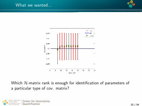
What we wanted...

Which H-matrix rank is enough for identification of parameters ofa particular type of cov. matrix?




23 / 54

4*

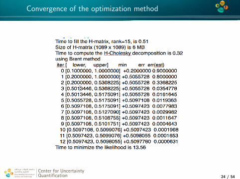
Convergence of the optimization method




24 / 54

4*

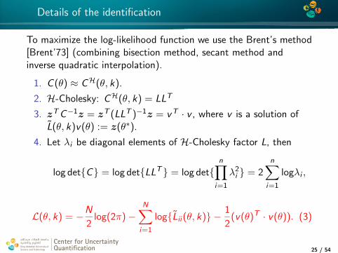
Details of the identification

To maximize the log-likelihood function we use the Brent’s method[Brent’73] (combining bisection method, secant method andinverse quadratic interpolation).

1. C (θ) ≈ CH(θ, k).

2. H-Cholesky: CH(θ, k) = LLT

3. zTC−1z = zT (LLT )−1z = vT · v , where v is a solution ofL(θ, k)v(θ) := z(θ∗).

4. Let λi be diagonal elements of H-Cholesky factor L, then

log detC = log detLLT = log detn∏

i=1

λ2i = 2

n∑i=1

logλi ,

L(θ, k) = −N

2log(2π)−

N∑i=1

logLii (θ, k) − 1

2(v(θ)T · v(θ)). (3)




25 / 54

0 10 20 30 40−4000

−3000

−2000

−1000

0

1000

2000

parameter θ, truth θ*=12

Log−

likelih

ood(θ

)

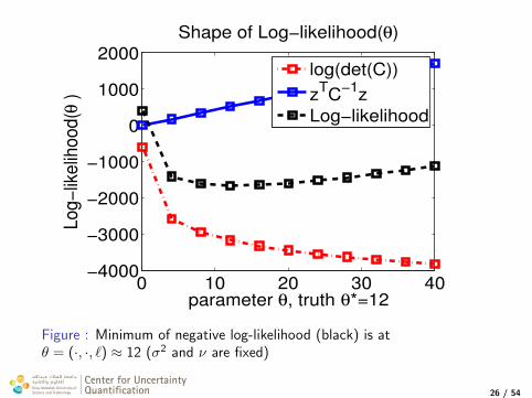
Shape of Log−likelihood(θ)

log(det(C))

zTC

−1z

Log−likelihood

Figure : Minimum of negative log-likelihood (black) is atθ = (·, ·, `) ≈ 12 (σ2 and ν are fixed)




26 / 54

4*

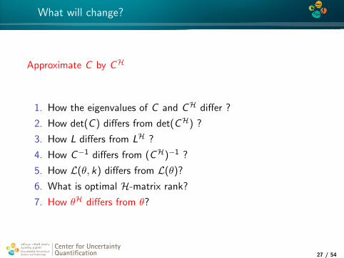
What will change?

Approximate C by CH

1. How the eigenvalues of C and CH differ ?

2. How det(C ) differs from det(CH) ?

3. How L differs from LH ?

4. How C−1 differs from (CH)−1 ?

5. How L(θ, k) differs from L(θ)?

6. What is optimal H-matrix rank?

7. How θH differs from θ?




27 / 54

4*

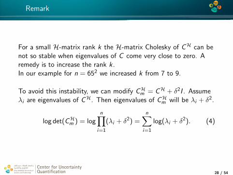
Remark

For a small H-matrix rank k the H-matrix Cholesky of CH can benot so stable when eigenvalues of C come very close to zero. Aremedy is to increase the rank k .In our example for n = 652 we increased k from 7 to 9.

To avoid this instability, we can modify CHm = CH + δ2I . Assumeλi are eigenvalues of CH. Then eigenvalues of CHm will be λi + δ2.

log det(CHm ) = logn∏

i=1

(λi + δ2) =n∑

i=1

log(λi + δ2). (4)




28 / 54

4*

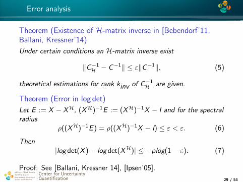
Error analysis

Theorem (Existence of H-matrix inverse in [Bebendorf’11,Ballani, Kressner’14)

Under certain conditions an H-matrix inverse exist

‖C−1H − C−1‖ ≤ ε‖C−1‖, (5)

theoretical estimations for rank kinv of C−1H are given.

Theorem (Error in log det)

Let E := X − XH, (XH)−1E := (XH)−1X − I and for the spectralradius

ρ((XH)−1E ) = ρ((XH)−1X − I) ≤ ε < ε. (6)

Then|log det(X )− log det(XH)| ≤ −plog(1− ε). (7)

Proof: See [Ballani, Kressner 14], [Ipsen’05].Center for UncertaintyQuantification



29 / 54

4*

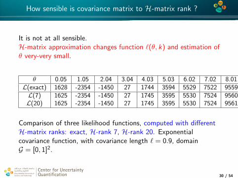
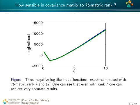
How sensible is covariance matrix to H-matrix rank ?

It is not at all sensible.H-matrix approximation changes function `(θ, k) and estimation ofθ very-very small.

θ 0.05 1.05 2.04 3.04 4.03 5.03 6.02 7.02 8.01 9 10L(exact) 1628 -2354 -1450 27 1744 3594 5529 7522 9559 11628 13727L(7) 1625 -2354 -1450 27 1745 3595 5530 7524 9560 11630 13726L(20) 1625 -2354 -1450 27 1745 3595 5530 7524 9561 11630 13725

Comparison of three likelihood functions, computed with differentH-matrix ranks: exact, H-rank 7, H-rank 20. Exponentialcovariance function, with covariance length ` = 0.9, domainG = [0, 1]2.




30 / 54

4*

How sensible is covariance matrix to H-matrix rank ?

0 5 10−5000

0

5000

10000

15000

θ

−lo

glik

elih

ood

Figure : Three negative log-likelihood functions: exact, commuted withH-matrix rank 7 and 17. One can see that even with rank 7 one canachieve very accurate results.




31 / 54

4*

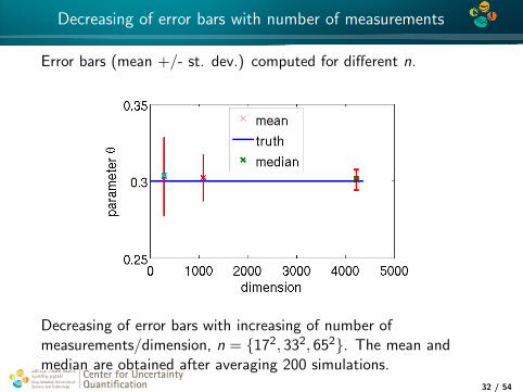
Decreasing of error bars with number of measurements

Error bars (mean +/- st. dev.) computed for different n.

Decreasing of error bars with increasing of number ofmeasurements/dimension, n = 172, 332, 652. The mean andmedian are obtained after averaging 200 simulations.




32 / 54

4*

Difference between two distributions, computed with C and CH

Kullback-Leibler divergence (KLD) DKL(P‖Q) is a measure of theinformation lost when distribution Q is used to approximate P:

DKL(P‖Q) =∑i

P(i) lnP(i)

Q(i), DKL(P‖Q) =

∫ ∞−∞

p(x) lnp(x)

q(x)dx ,

where p, q densities of P and Q. For multi-variate normaldistributions (µ0,Σ0) and (µ1,Σ1)

2DKL(N0‖N1) = tr(Σ−11 Σ0)+(µ1−µ0)TΣ−1

1 (µ1−µ0)−k− ln

(det Σ0

det Σ1

)




33 / 54

4*

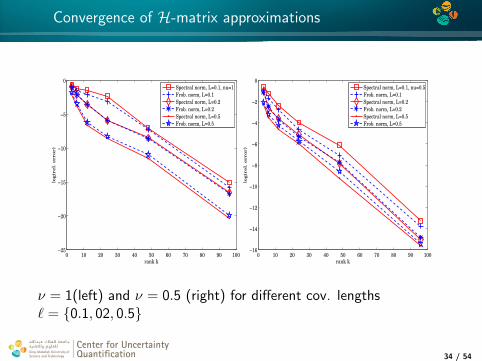
Convergence of H-matrix approximations

0 10 20 30 40 50 60 70 80 90 100−25

−20

−15

−10

−5

0

rank k

log(r

el.

error)

Spectral norm, L=0.1, nu=1

Frob. norm, L=0.1

Spectral norm, L=0.2

Frob. norm, L=0.2


Frob. norm, L=0.5

0 10 20 30 40 50 60 70 80 90 100−16

−14

−12

−10

−8

−6

−4

−2

0

rank k

log(r

el.

error)

Spectral norm, L=0.1, nu=0.5

Frob. norm, L=0.1


Frob. norm, L=0.2


Frob. norm, L=0.5

ν = 1(left) and ν = 0.5 (right) for different cov. lengths` = 0.1, 02, 0.5




34 / 54

4*

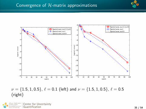
Convergence of H-matrix approximations

0 10 20 30 40 50 60 70 80 90 100−16

−14

−12

−10

−8

−6

−4

−2

0

rank k

log(r

el.

error)

Spectral norm, nu=1.5, L=0.1

Spectral norm, nu=1

Spectral norm, nu=0.5

0 10 20 30 40 50 60 70 80 90 100−22

−20

−18

−16

−14

−12

−10

−8

−6

−4

−2

rank k

log(r

el.

error)

Spectral norm, nu=1.5, L=0.5

Spectral norm, nu=1

Spectral norm, nu=0.5

ν = 1.5, 1, 0.5, ` = 0.1 (left) and ν = 1.5, 1, 0.5, ` = 0.5(right)




35 / 54

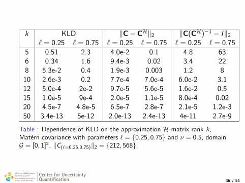
k KLD ‖C− CH‖2 ‖C(CH)−1 − I‖2

` = 0.25 ` = 0.75 ` = 0.25 ` = 0.75 ` = 0.25 ` = 0.75

5 0.51 2.3 4.0e-2 0.1 4.8 636 0.34 1.6 9.4e-3 0.02 3.4 228 5.3e-2 0.4 1.9e-3 0.003 1.2 8

10 2.6e-3 0.2 7.7e-4 7.0e-4 6.0e-2 3.112 5.0e-4 2e-2 9.7e-5 5.6e-5 1.6e-2 0.515 1.0e-5 9e-4 2.0e-5 1.1e-5 8.0e-4 0.0220 4.5e-7 4.8e-5 6.5e-7 2.8e-7 2.1e-5 1.2e-350 3.4e-13 5e-12 2.0e-13 2.4e-13 4e-11 2.7e-9

Table : Dependence of KLD on the approximation H-matrix rank k,Matern covariance with parameters ` = 0.25, 0.75 and ν = 0.5, domainG = [0, 1]2, ‖C(`=0.25,0.75)‖2 = 212, 568.




36 / 54

4*

Conclusion

I Covariance matrices can be approximated in H-matrix format.

I Influence of H-matrix approximation error on the estimatedparameters is small.

I With application of H-matricesI we extend the class of covariance functions to work with,I allows non-regular discretization of the covariance function on

large spatial grids.

I With the maximizing algorithm we are able to identify bothparameters: covariance lengths ` and the smoothness ν




37 / 54

4*

Future plans

I ECRC, center of D. Keyes: Parallel H-Cholesky on differentarchitectures → very large covariance matrices on complicategrids

I Apply H-matrices for

1. Kriging estimate s := CsyC−1yy y

2. Estimation of variance σ, is the diagonal of conditional cov.matrix Css|y = diag

(Css − CsyC−1

yy Cys

),

3. Gestatistical optimal design ϕA := n−1traceCss|y ,

ϕC := cT(Css − CsyC−1

yy Cys

)c ,

I Identify all three parameters (σ2, `, ν) simultaneously

I Compare with the Bayesian Update (H. Matthies, H. Najm,K. Law, A. Stuart et al)




38 / 54

4*

Literature

1. PCE of random coefficients and the solution of stochastic partialdifferential equations in the Tensor Train format, S. Dolgov, B. N.Khoromskij, A. Litvinenko, H. G. Matthies, 2015/3/11, arXiv:1503.032102. Efficient analysis of high dimensional data in tensor formats, M. Espig,W. Hackbusch, A. Litvinenko, H.G. Matthies, E. Zander Sparse Grids andApplications, 31-56, 40, 20133. Application of hierarchical matrices for computing the Karhunen-Loeveexpansion, B.N. Khoromskij, A. Litvinenko, H.G. Matthies, Computing84 (1-2), 49-67, 31, 20094. Efficient low-rank approximation of the stochastic Galerkin matrix intensor formats, M. Espig, W. Hackbusch, A. Litvinenko, H.G. Matthies,P. Waehnert, Comp. & Math. with Appl. 67 (4), 818-829, 2012

5. Numerical Methods for Uncertainty Quantification and Bayesian

Update in Aerodynamics, A. Litvinenko, H. G. Matthies, Book

”Management and Minimisation of Uncertainties and Errors in Numerical

Aerodynamics” pp 265-282, 2013




39 / 54

4*

Acknowledgement

1. Lars Grasedyck (RWTH Aachen) and Steffen Boerm (UniKiel) for HLIB (www.hlib.org)

2. KAUST Research Computing group, KAUST SupercomputingLab (KSL)

3. Stochastic Galerkin library (sglib from E. Zander). Type inyour terminalgit clone git://github.com/ezander/sglib.git

To initialize all variables, run startup.m You will find:generalised PCE, sparse grids, (Q)MC, stochastic Galerkin, linearsolvers, KLE, covariance matrices, statistics, quadratures(multivariate Chebyshev, Laguerre, Lagrange, Hermite ) etc

There are: many examples, many test, rich demos




40 / 54

4*

Additional information

Additional information




41 / 54

4*

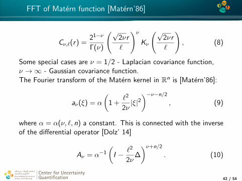
FFT of Matern function [Matern’86]

Cν,`(r) =21−ν

Γ(ν)

(√2νr

`

)νKν

(√2νr

`

), (8)

Some special cases are ν = 1/2 - Laplacian covariance function,ν →∞ - Gaussian covariance function.The Fourier transform of the Matern kernel in Rn is [Matern’86]:

aν(ξ) = α

(1 +

`2

2ν|ξ|2)−ν−n/2

, (9)

where α = α(ν, `, n) a constant. This is connected with the inverseof the differential operator [Dolz’ 14]

Aν = α−1

(I − `2

2ν∆

)ν+n/2

. (10)




42 / 54

4*

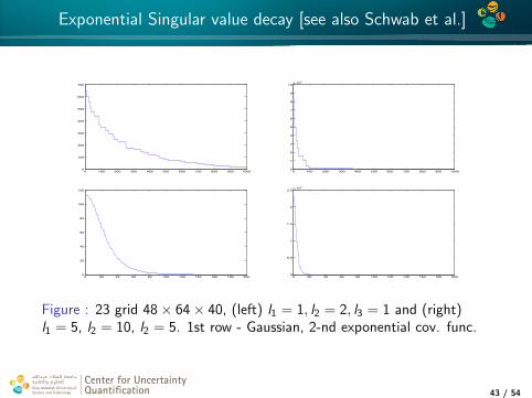
Exponential Singular value decay [see also Schwab et al.]

0 100 200 300 400 500 600 700 800 900 10000

100

200

300

400

500

600

700

0 100 200 300 400 500 600 700 800 900 10000

1

2

3

4

5

6

7

8

9

10x 10

4

0 20 40 60 80 100 120 140 160 180 2000

20

40

60

80

100

120

0 20 40 60 80 100 120 140 160 180 2000

0.5

1

1.5

2

2.5x 10

4

Figure : 23 grid 48× 64× 40, (left) l1 = 1, l2 = 2, l3 = 1 and (right)l1 = 5, l2 = 10, l2 = 5. 1st row - Gaussian, 2-nd exponential cov. func.




43 / 54

4*

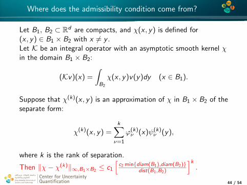
Where does the admissibility condition come from?

Let B1, B2 ⊂ Rd are compacts, and χ(x , y) is defined for(x , y) ∈ B1 × B2 with x 6= y .Let K be an integral operator with an asymptotic smooth kernel χin the domain B1 × B2:

(Kv)(x) =

∫B2

χ(x , y)v(y)dy (x ∈ B1).

Suppose that χ(k)(x , y) is an approximation of χ in B1 × B2 of theseparate form:

χ(k)(x , y) =k∑ν=1

ϕ(k)ν (x)ψ(k)

ν (y),

where k is the rank of separation.

Then ‖χ− χ(k)‖∞,B1×B2 ≤ c1

[c2 mindiam(B1),diam(B2)

dist(B1,B2)

]k.




44 / 54

4*

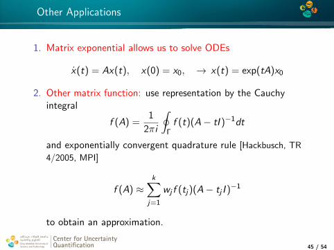
Other Applications

1. Matrix exponential allows us to solve ODEs

x(t) = Ax(t), x(0) = x0, → x(t) = exp(tA)x0

2. Other matrix function: use representation by the Cauchyintegral

f (A) =1

2πi

∮Γ

f (t)(A− tI )−1dt

and exponentially convergent quadrature rule [Hackbusch, TR

4/2005, MPI]

f (A) ≈k∑

j=1

wj f (tj)(A− tj I )−1

to obtain an approximation.




45 / 54

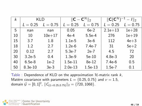
k KLD ‖C− CH‖2 ‖C(CH)−1 − I‖2

L = 0.25 L = 0.75 L = 0.25 L = 0.75 L = 0.25 L = 0.75

5 nan nan 0.05 6e-2 2.1e+13 1e+2810 10 10e+17 4e-4 5.5e-4 276 1e+1915 3.7 1.8 1.1e-5 3e-6 112 4e+318 1.2 2.7 1.2e-6 7.4e-7 31 5e+220 0.12 2.7 5.3e-7 2e-7 4.5 7230 3.2e-5 0.4 1.3e-9 5e-10 4.8e-3 2040 6.5e-8 1e-2 1.5e-11 8e-12 7.4e-6 0.550 8.3e-10 3e-3 2.0e-13 1.5e-13 1.5e-7 0.1

Table : Dependence of KLD on the approximation H-matrix rank k,Matern covariance with parameters L = 0.25, 0.75 and ν = 1.5,domain G = [0, 1]2, ‖C(L=0.25,0.75)‖2 = 720, 1068.




46 / 54

4*

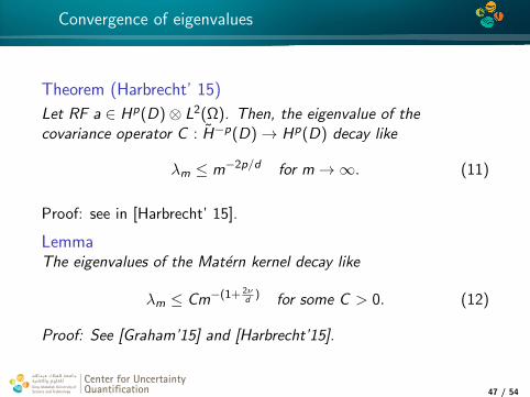
Convergence of eigenvalues

Theorem (Harbrecht’ 15)

Let RF a ∈ Hp(D)⊗ L2(Ω). Then, the eigenvalue of thecovariance operator C : H−p(D)→ Hp(D) decay like

λm ≤ m−2p/d for m→∞. (11)

Proof: see in [Harbrecht’ 15].

LemmaThe eigenvalues of the Matern kernel decay like

λm ≤ Cm−(1+ 2νd

) for some C > 0. (12)

Proof: See [Graham’15] and [Harbrecht’15].




47 / 54

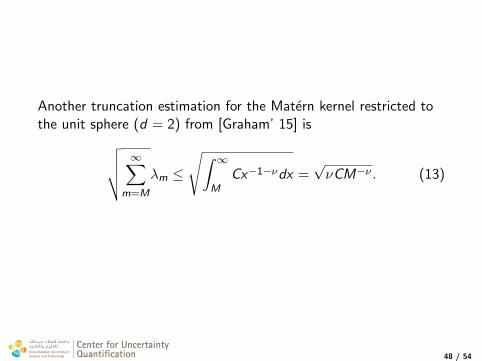
Another truncation estimation for the Matern kernel restricted tothe unit sphere (d = 2) from [Graham’ 15] is√√√√ ∞∑

m=M

λm ≤

√∫ ∞M

Cx−1−νdx =√νCM−ν . (13)




48 / 54

4*

Matern Fields (Whittle, 63)

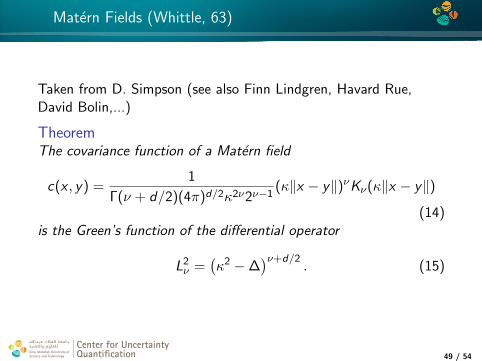
Taken from D. Simpson (see also Finn Lindgren, Havard Rue,David Bolin,...)

TheoremThe covariance function of a Matern field

c(x , y) =1

Γ(ν + d/2)(4π)d/2κ2ν2ν−1(κ‖x − y‖)νKν(κ‖x − y‖)

(14)is the Green’s function of the differential operator

L2ν =

(κ2 −∆

)ν+d/2. (15)




49 / 54

4*

Gaussian Field and Green Function

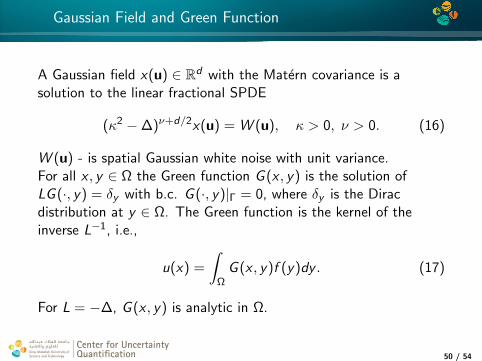
A Gaussian field x(u) ∈ Rd with the Matern covariance is asolution to the linear fractional SPDE

(κ2 −∆)ν+d/2x(u) = W (u), κ > 0, ν > 0. (16)

W (u) - is spatial Gaussian white noise with unit variance.For all x , y ∈ Ω the Green function G (x , y) is the solution ofLG (·, y) = δy with b.c. G (·, y)|Γ = 0, where δy is the Diracdistribution at y ∈ Ω. The Green function is the kernel of theinverse L−1, i.e.,

u(x) =

∫Ω

G (x , y)f (y)dy . (17)

For L = −∆, G (x , y) is analytic in Ω.




50 / 54

4*

Bridge between numerical methods for PDEs and covariance

How we can use this bridge between numerical methods for PDEsand covariance ?See, e.g. [Bebendorf, Hackbusch 02,] Existence of H-matrixapproximation of the inverse FE-matrix of elliptic operators withL∞-coefficients. The Green functions of uniformly elliptic operatorcan be approximated by degenerate functions giving rise to theexistence of blockwise low-rank approximants of FEM inverses.




51 / 54

4*

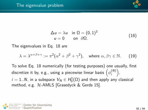
The eigenvalue problem

∆u = λu in Ω = (0, 1)3

u = 0 on ∂Ω.(18)

The eigenvalues in Eq. 18 are

λ = λα+β+γ := π2(α2 + β2 + γ2), where α, βγ ∈ N. (19)

To solve Eq. 18 numerically (for testing purposes) one usually, first

discretize it by, e.g., using a piecewise linear basis(φ

(N)i

),

i = 1..N, in a subspace VN ∈ H10 (Ω) and then apply any classical

method, e.g. H-AMLS [Grasedyck & Gerds 15].




52 / 54

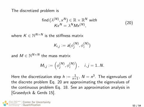
The discretized problem is

find (λ(N), xN) ∈ R× RN with

KxN = λNMx (N),(20)

where K ∈ NN×N is the stiffness matrix

Ki ,j := a(φ(N)j , φ

(N)i )

and M ∈ NN×N the mass matrix

Mi ,j :=(φ

(N)j , φ

(N)i

), i , j = 1..N.

Here the discretization step h := 1n+1 , N = n3. The eigenvalues of

the discrete problem Eq. 20 are approximating the eigenvalues ofthe continuous problem Eq. 18. See an approximation analysis in[Grasedyck & Gerds 15].




53 / 54

4*

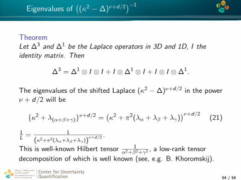
Eigenvalues of((κ2 −∆)ν+d/2

)−1

TheoremLet ∆3 and ∆1 be the Laplace operators in 3D and 1D, I theidentity matrix. Then

∆3 = ∆1 ⊗ I ⊗ I + I ⊗∆1 ⊗ I + I ⊗ I ⊗∆1.

The eigenvalues of the shifted Laplace (κ2 −∆)ν+d/2 in the powerν + d/2 will be

κ2 + λ(α+β+γ)ν+d/2 =(κ2 + π2(λα + λβ + λγ)

)ν+d/2(21)

1L = 1

(κ2+π2(λα+λβ+λγ))ν+d/2 .

This is well-known Hilbert tensor 1α2+β2+γ2 , a low-rank tensor

decomposition of which is well known (see, e.g. B. Khoromskij).




54 / 54

Alexander Litvinenko, Quanti cation Center, KAUST · PDF fileFast and cheap approximation of...

Documents

Transcript of Alexander Litvinenko, Quanti cation Center, KAUST · PDF fileFast and cheap approximation of...