
Agi4x44PreProcess
29
Agi4x44Preprocess Pedro Lopez-Romero October 31, 2011 1 Package Overview The Agi4x44PreProcess package has been designed to read Agilent 4 x 44 gene expression arrays data files into R [3] for its pre-processing using other Biocon- ductor functions. The package needs plain text files exported by the Agilent Feature Extraction 9.1.3.1 (or later version) image analysis software (AFE) [1]. The pre-processing steps implemented in the package are the following: 1.- read the target file 2.- read the array samples 3.- Background correction and Normalization between samples 4.- Filtering Probes by Quality Flag 5.- Summarizing of Replicated Probes 6.- Creating and ExpressionSet object with the processed data The package also contains other utilities that allow the user to explore the architecture of the chip in terms of probe replication and gene replication. Agi4x44PreProcess contains standard graphical utilities to evaluate the qual- ity of the data. These graphics might help the users to decide what sort fore- ground and background signal, amongst those provided by the AFE, they want to use in their analysis, and what background signal correction and normaliza- tion method between samples they want to perform. Finally, Agi4x44PreProcess also generates the files DataSet.gct and Pheno- types.cls that are used by the Gene Set Enrichment Analysis tool (GSEA) [5]. Agi4x44PreProcess employees the corresponding Bioconductor annotation packages (human: ”hgug4112a.db”; mouse: ”mgug4122a.db”) to assign to each probe the ACCNUM, SYMBOL, ENTREZID, DESCRIPTION, GO TERMS AND GO IDS. The annotacion package that is going to be used should be loaded into the R session. In our example we used the hgug4112a.db annotation package. The annotation package can be loaded using library > library("hgug4112a.db") The package allows choosing between different alternatives in each of the pre- processing steps. Currently only the plain text files exported by AFE are sup- ported. To read these files into R the Rpackagelimma function read.maimages [4] is used. The user can choose the foreground signal (gProcessedSignal or gMeanSignal) and the background signal for the background correction (gBG- MedianSignal or gBGUsed). It also decides the methods for the Background 1
description
hummm
Transcript of Agi4x44PreProcess

Agi4x44Preprocess
Pedro Lopez-Romero
October 31, 2011
1 Package Overview
The Agi4x44PreProcess package has been designed to read Agilent 4 x 44 geneexpression arrays data files into R [3] for its pre-processing using other Biocon-ductor functions. The package needs plain text files exported by the AgilentFeature Extraction 9.1.3.1 (or later version) image analysis software (AFE) [1].The pre-processing steps implemented in the package are the following:
1.- read the target file 2.- read the array samples 3.- Background correctionand Normalization between samples 4.- Filtering Probes by Quality Flag 5.-Summarizing of Replicated Probes 6.- Creating and ExpressionSet object withthe processed data
The package also contains other utilities that allow the user to explore thearchitecture of the chip in terms of probe replication and gene replication.
Agi4x44PreProcess contains standard graphical utilities to evaluate the qual-ity of the data. These graphics might help the users to decide what sort fore-ground and background signal, amongst those provided by the AFE, they wantto use in their analysis, and what background signal correction and normaliza-tion method between samples they want to perform.
Finally, Agi4x44PreProcess also generates the files DataSet.gct and Pheno-types.cls that are used by the Gene Set Enrichment Analysis tool (GSEA) [5].
Agi4x44PreProcess employees the corresponding Bioconductor annotationpackages (human: ”hgug4112a.db”; mouse: ”mgug4122a.db”) to assign to eachprobe the ACCNUM, SYMBOL, ENTREZID, DESCRIPTION, GO TERMSAND GO IDS. The annotacion package that is going to be used should beloaded into the R session. In our example we used the hgug4112a.db annotationpackage. The annotation package can be loaded using library
> library("hgug4112a.db")
The package allows choosing between different alternatives in each of the pre-processing steps. Currently only the plain text files exported by AFE are sup-ported. To read these files into R the Rpackagelimma function read.maimages
[4] is used. The user can choose the foreground signal (gProcessedSignal orgMeanSignal) and the background signal for the background correction (gBG-MedianSignal or gBGUsed). It also decides the methods for the Background
1

correction (”none”, ”half”, ”normexp”) and for the Normalization between ar-rays (”none”, ”quantile”, ”vsn”). The backgroundCorrect and normalizeBe-
tweenArrays Rpackagelimma functions [4] have been used. If the user wantsto use other methods implemented in backgroundCorrect and in normalize-
BetweenArrays but not incorporated in the Agi4x44PreProcess package, theycan easily call any of these functions externally. The users also choose if theywant to filter out the probes that do not reach a minimum of quality, which isalso established by the user. In this sense we can be more or less demanding infunction of the data in hand (low number of replicates probably demands beingmore restrictive about quality limits). There is a final summarization step thatcollapse the non-control replicated probes into a single value. The users can alsoskip the Summarization step in order to use all the probes being replicated ornot. Finally the processed data is stored in an RGList that can be transformedinto an ExpressionSet. The ExpressionSet object can be used to statisticallyanalyze the data (differential expression, functional analysis, etc) using otheranalytical packages such as limma.
2 Target File
We have to specify the experimental conditions under which the data have beengenerated in a target file, where each sample is related with an experimentalgroup. This is done in a plain text file that can be loaded into R using theAgi4x44PreProcess function read.targets.
First we load the package and then we read the target file
# NOT RUN #
> library("Agi4x44PreProcess")
> targets=read.targets(infile="targets.txt")
# NOT RUN #
The function read.target returns a data.frame object similar to this:
> library("Agi4x44PreProcess")
> data(targets)
> targets
FileName Treatment GErep Subject Array
Ast Ast.txt st 1 A 1
Bst Bst.txt st 1 B 1
Aunst Aunst.txt unst 2 A 1
Bunst Bunst.txt unst 2 B 1
In the target file, the fields Filename, Treatment and GErep are mandatory.The Filename specifies the name of the files, the Treatment specify which level of
2

the treatment corresponds the FileName. Other variables might also be includedif the users want to use them in further downstream statistical analysis. In ourgiven example, we have human cells that have been treated with BMP2 that areto be compared with untreated cells, so in our design we consider a Treatmenteffect with two levels, Stimulated and Unstimulated. We have collected tworeplicates of each treatment level and both treatments have been applied tocells of the same individuals, that is, the design have been blocked by Subject.As we only have two levels of the blocking variable subject, this kind of designis normally known as a paired design. To consider the paired design in futuredownstream analysis, using limma for instance, we have to add a subject variablethat relates the individual with its sample. The GErep is a redundant variablethat mirrors the Treatment variable using a numeric code, i.e., each treatmentlevel (Stimulated an Unstimulated) is also codified numerically by being n thenumber of levels of the treatment effect. We have included the Array variable asan example of other sort of variables that we may want to use. In this case, theArray variable refers to platform where the sample has been hybridized. Recallthat the Agilent 4x44 platforms allows the hybridization of 4 different samplesonto the same platform. In our example, as long as we have only 4 sampleshybridized on the same platform the inclusion of this variable does not makeany sense, since all the samples have been hybridized on the same platform, butif we had more samples hybridized on different platforms we could consider theplatform (Array) as a blocking variable, using designs such as complete blockdesigns or incomplete block designs.
3 Reading the data
The chips were scanned using the Agilent G2567AA Microarray Scanner Sys-tem (Agilent Technologies) with the extended dynamic range option turned on.Image analysis and data collection were carried out using the Agilent FeatureExtraction 9.1.3.1. (AFE) [1]. For the background signal the AFE was set touse the spatial detrend surface value that estimate the noise due to a systematicgradient on the array and whose computation is based on a Loess algorithm.Details of how the spatial detrend algorithm works can be found in the AFEreference guide.
Currently only the plain text files exported by AFE are supported. Toread these files into R the limma function [4] read.maimages is used. In ourexample, use real data from Agilent 4x44 Human chips. However, for the sakeof reducing the disk space storing the original data have been trimmed, leaving12,015 features out of the 45,015 that should be found on a Human Agilent4x44 chip. Despite of this, the data example is perfectly valid to illustrate allthe features and performance of the functions included in the package, althoughsome of the functions regarding counting replicated probes, etc will producenumbers that will not coincide with the real data.
To read the files we use the read.AgilentFE function:
3

# NOT RUN #
> dd=read.AgilentFE(targets, makePLOT=FALSE)
# NOT RUN #
The result will be an RGList similar to this:
> data(dd)
> class(dd)
[1] "RGList"
attr(,"package")
[1] "limma"
> dim(dd)
[1] 12015 4
The RGList contains the following slots
> names(dd)
[1] "R" "G" "Rb" "Gb" "targets" "genes" "other"
The data stored in the RGList are the following:
variable datadd$R gProcessedSignaldd$G gMeanSignaldd$Rb gBGMedianSignaldd$Gb gBGUsed
dd$targets File namesdd$genes$ProbeName Probe Namedd$genes$GeneName Gene Name
dd$genes$SystematicName Systematic Namedd$genes$Description Description Namedd$genes$Sequence 60 bases Sequence
dd$genes$ControlType FLAG to specify the sort of featuredd$other$gIsWellAboveBG FLAG IsWellAboveBG
dd$other$gIsFound FLAG IsFounddd$other$gIsSaturated FLAG IsSaturated
dd$other$gIsFeatPopnOL FLAG IsFeatPopnOLdd$other$gIsFeatNonUnifOL FLAG IsFeatNonUnifOL
dd$other$chr coord CHR coordinate from Agilent data files
4
The MeanSignal is the Raw mean signal of the spot. The ProcessedSig-nal is the signal processed by AFE [1]. It contains the Multiplicatively De-trend Background Subtracted Signal if the detrending is selected and it helps.If the detrending does not help, the ProcessedSignal will be the BackgroundSubtracted Signal. The BGMedianSignal is the Median local background sig-nal. The BGUsed depends on the scanner settings for the type of backgroundmethod and the setting for the spatial detrend. Usually, the Background Sig-nal Used is the sum of the local background + the spatial detrending surfacevalue computed by the AFE software. To view the values used to calculate thisvariable using different background signals and settings of spatial detrend andglobal background adjust [1].
The dd$targets contain the name of the files equal to those in target file. Thedd$genes$ProbeName, dd$genes$GeneName, dd$genes$SystematicName, anddd$genes$Description provide the mappings to dd$genes$ProbeName accordingto Agilent. In the Agi4x44PreProcess, if an annotation package exists, the fieldsSystematicName, GeneName and Description are replaced, respectively, by thecorresponding ACCNUM, SYMBOL and DESCRIPTION obtained from thecorresponding annotation package.
The AFE attach to each feature a flag that identifies different quantificationerrors of the signal. These quantification flags can be used to filter out signalsthat do not reach a minimum established criterion of quality. We will come backagain to the filtering process in the section 8.
The dd$other$chr coord variable contains the chromosomal coordinates pro-vided by the Agilent manufacturer. These coordinates are used by the functiongenes.rpt.agi to create links to the ENSEMBL data base for the different probesinterrogating the same gene. See section 6.
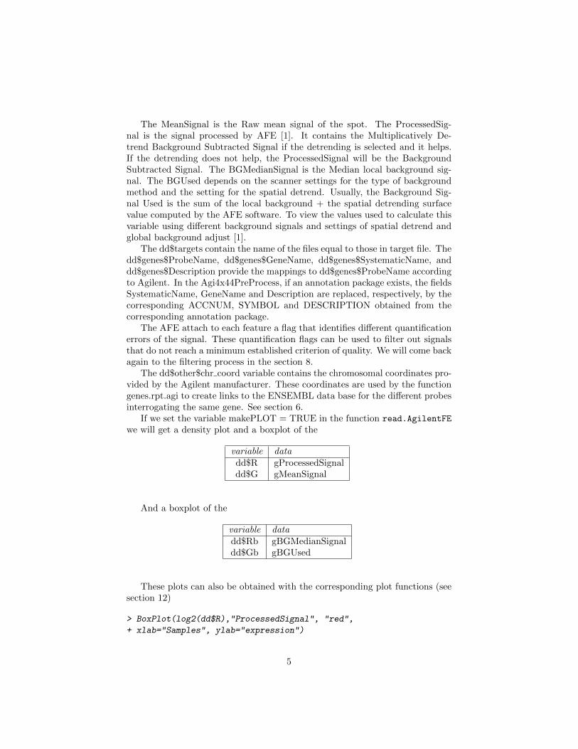
If we set the variable makePLOT = TRUE in the function read.AgilentFE
we will get a density plot and a boxplot of the
variable datadd$R gProcessedSignaldd$G gMeanSignal
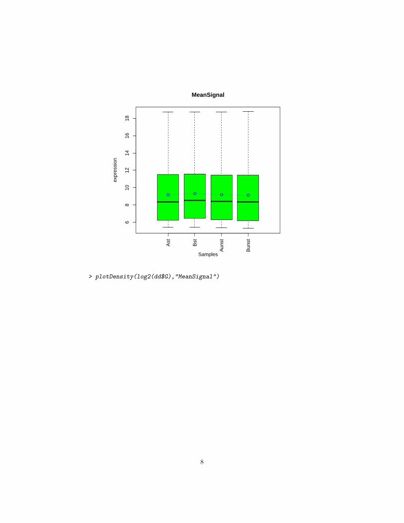
And a boxplot of the
variable datadd$Rb gBGMedianSignaldd$Gb gBGUsed
These plots can also be obtained with the corresponding plot functions (seesection 12)
> BoxPlot(log2(dd$R),"ProcessedSignal", "red",
+ xlab="Samples", ylab="expression")
5

● ● ● ●
Samples
expr
essi
on
Ast
Bst
Aun
st
Bun
st
510
15
● ● ● ●
ProcessedSignal
> plotDensity(log2(dd$R),"ProcessedSignal")
6

5 10 15 20
0.00
0.05
0.10
0.15
0.20
N = 12015 Bandwidth = 0.5587
Den
sity
ProcessedSignal
AstBstAunstBunst
> BoxPlot(log2(dd$G),"MeanSignal", "green",
+ xlab="Samples", ylab="expression")
7
● ● ● ●
Samples
expr
essi
on
Ast
Bst
Aun
st
Bun
st
68
1012
1416
18
● ● ● ●
MeanSignal
> plotDensity(log2(dd$G),"MeanSignal")
8

5 10 15 20
0.00
0.05
0.10
0.15
0.20
0.25
N = 12015 Bandwidth = 0.4342
Den
sity
MeanSignal
AstBstAunstBunst
> BoxPlot(log2(dd$Gb),"BGUsed", "orange",
+ xlab="Samples", ylab="expression")
9
●●
●
●
Samples
expr
essi
on
●●●●●●●●●●●●●●●●●●●
●●●●
●●●●
●●●●●
●●●
●●
●●●
●●
●●●
●●●
●●●
●●●
●●●●●
●●●●●●
●●●●
●●●
●●●●
●●●
●●●●
●●●
●●●●
●●●
●●●●
●●●
●●●●
●●●●
●●●●
●●●●
●●●●
●●●●
●●●●
●●●●
●●●●
●●●●
●●●●●●●●●●●●●●●●●●●●●●●●●●●●●●●●●●●●●●●●●●●●●●●●
●●●●●●●●●●●●●●●●●●●●●●●●●●●●●●●●●●●●●●●●●●●●●●●●
●●●●●●●●●●●●●●●●●●●●●●●●●●●●●●●●●●●●●●●●●●●●●●●
●●●●●●●●●●●●●●●●●●●●●●●●●●●●●●●●●●●●●●●●●●●●●●●●
●●●●●●●●●●●●●●●●●●●●●●●●●●●●●●●●●●●●●●●●●●●●●●●●
●●●●●●●●●●●●●●●●●●●●●●●●●●●●●●●●●●●●●●●●●●●●●●
●●●●●●●●●●●●●●●●●●●●●●●●●●●●●●●●●●●●●●●●●●●●●●●●
●●●●●●●●●●●●●●●●●●●●●●●●●●●●●●●●●●●●●●●●●●●●●●●
●●●●●●●●●●●●●●●●●●●●●●●●●●●●●●●●●●●●●●●●●●●●●●●●
●●●●●●●●●●●●●●●●●●●●●●●●●●●●●●●●●●●●●●●●●●●●●●●
●●●●●●●●●●●●●●●●●●●●●●●●●●●●●●●●●●●●●●●●●●●●●●●●
●●●●●●●●●●●●●●●●●●●●●●●●●●●●●●●●●●●●●●●●●●●●●●
●●●●●●●●●●●●●●●●●●
●●●●●●●●●●●●●●●●●
●●●●●●●●●●●●●●●●●
●●●●●●●●●●●●●●●●●
●●●●●●●●●●●●●●●●●
●●●●●●●●●●●●●●●●
●●●●●●●●●●●●●●●●●
●●●●●●●●●●●●●●●●●
●●●●●●●●●●●●●●●●●
●●●●●●●●●●●●●●●●
●●●●●●●●●●●●●●●●●
●●●●●●●●●●●●●●●●
Ast
Bst
Aun
st
Bun
st
5.9
6.0
6.1
6.2
6.3
●●
●
●
BGUsed
> BoxPlot(log2(dd$Rb),"BGMedianSignal", "blue",
+ xlab="Samples", ylab="expression")
10

● ● ● ●
Samples
expr
essi
on
●
●●●●●●●●●●●●●●●●●●●●●●●●●●●●●●●●●●●●●●●●●●●●●●●●●●●●●●●●●●
●●●●●●●●●●●●●●●
●●●●●●●●●●●●●●●●●●●●●●●●●●●●●●●●●
●
●●●●●●●●●
●
●●
●
●
●
●
●
●
●
●●
●
●●●●●●●●●●●●●
●●
●●
●
●
●
●●●
●
●
●●
●●
●
●●
●
●
●
●●●●●●●●●●●●●●●●●●●●●●●●●●●●●●●●●●●●
●
●●●●●●●●●●●●●●●●●●●●●●●●●●●●●●●●●●●●●●●●●●●●●●●●●●●
●
●●
●●●●●●●●●●●●●●●●●●●●
●
●●●●
●●●●●●●●●●●●●●●●●●●●●●●●●●●●●●●●●●●●●●●●●●●●●●●●●●●●●●●●●●
●
●●
●
●●●●●
●●●
●●●●●●●●●●●●●
●
●●●●●●●●●●●●●●●●●●●●●●●●
●
●
●
●●●
●
●●
●
●
●●●
●
●
●●
●
●
●●●●●●●●●●●●●●●●●●
●●●●●●●●●●
●●●●●●●●●●●●●●●●●●●●●●●●●●●●●●●●●●●●●●●●●●●
●●●●●●●●●●●●
●
●●●●●●●●●●
●
●●●●●●
●
●●
●
●●●●●
●
●●●●●●●●●●●●●●●
●
●●●●●●●●●●
●
●●●●●●●●●●
●●●●●●●●●
●
●●●
●
●●●
●
●●●●●●
●
●
●
●
●
●
●●
●
●●●
●
●
●
Ast
Bst
Aun
st
Bun
st
46
810
1214
16
● ● ● ●
BGMedianSignal
4 Replicated Probes
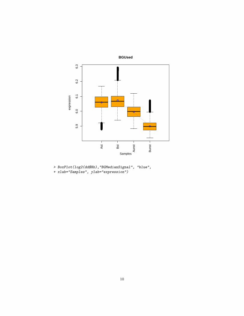
The Agilent arrays contains a number of non-control probes replicated up toten times which are spread across the array. This allows computing the %CV (percent of the coefficient of variation) for each array. Agi4x44PreProcessincorporates a specific function, CV.rep.probes, that allows the identification ofthe non-control replicated probes (we call them Probe Sets) and the computationof their coefficient of variation (% CV). The CV is computed for every set ofreplicated probes. Within each array, the median of the CV of every probe-set is reported as the CV of the array. A lower median CV indicates a betterreproducibility of the array. The CV can be used as a measured of the qualityof the arrays and it can help to detect a sample that deviates from the rest asan erroneous one. This measure is also reported by the QC report of AFE. TheCV.rep.probes function also writes a file (Probe.Sets.txt) that contains the non-control replicated probes, along with its PROBE ID, the number of replicates,the ACCNUM code, the SYMBOL code, the DESCRIPTION of the gene, andthe % CV of the probe in each array. The CVs are also given in a boxplot.
> CV.rep.probes(dd,"hgug4112a.db",
+ foreground="MeanSignal", raw.data=TRUE,
+ writeR=FALSE, targets)
11
------------------------------------------------------
Non-CTRL Replicated probes
foreground: MeanSignal
FILTERING BY ControlType FLAG
RAW DATA: PROBES AFTER ControlType FILTERING: 11259
------------------------------------------------------
REPLICATED NonCtrl Probes 207
UNIQUE probes 10836
DISTRIBUTION OF REPLICATED NonControl Probes
reps
1 2 3 4 5
79 63 46 15 4
# REPLICATED (redundant) probeNames 423
------------------------------------------------------
MEDIAN % CV
Ast Bst Aunst Bunst
1.041 0.878 0.948 1.107
------------------------------------------------------
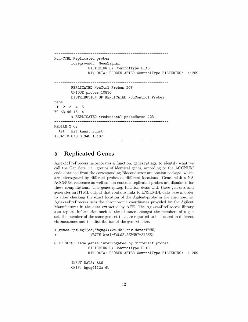
5 Replicated Genes
Agi4x44PreProcess incorporates a function, genes.rpt.agi, to identify what wecall the Gen Sets, i.e. groups of identical genes, according to the ACCNUMcode obtained from the corresponding Bioconductor annotation package, whichare interrogated by different probes at different locations. Genes with a NAACCNUM reference as well as non-controls replicated probes are dismissed forthese computations. The genes.rpt.agi function deals with these gen-sets andgenerates an HTML output that contains links to ENSEMBL data base in orderto allow checking the exact location of the Agilent-probe in the chromosome.Agi4x44PreProcess uses the chromosome coordinates provided by the AgilentManufacturer in the data extracted by AFE. The Agi4x44PreProcess libraryalso reports information such as the distance amongst the members of a genset, the member of the same gen set that are reported to be located in differentchromosomes and the distribution of the gen sets size.
> genes.rpt.agi(dd,"hgug4112a.db",raw.data=TRUE,
+ WRITE.html=FALSE,REPORT=FALSE)
GENE SETS: same genes interrogated by different probes
FILTERING BY ControlType FLAG
RAW DATA: PROBES AFTER ControlType FILTERING: 11259
INPUT DATA: RAW
CHIP: hgug4112a.db
12

PROBE SETS (NON-CTRL prob rep. x 10): 207
GEN-SETS (REPLICATED GENES): 537
PROBES in gen-sets: 1115
Be aware that may be non-control replicated probes that interrogate thesame gene in the same location, and the very same gene might be interrogatedby other probe at different chromosomal location.
6 Background Correction and Normalization be-tween arrays
To make direct comparisons of data coming from different chips it is importantto remove sources of variation of non biological nature that may exists betweenarrays. Systematic non-biological differences between chips become apparentin several obvious ways especially in labelling and in hybridization, and biasthe relative measures on any two chips when we want to quantify the differ-ences in treatment of two samples. Normalization is the attempt to compensatefor systematic technical differences between chips, to see more clearly the sys-tematic biological differences between samples. First the data are backgroundcorrected. We produced a Background Subtracted Signal. The Background Sig-nal Used depends on the scanner settings for the type of background methodand the settings for spatial detrend. Usually, the Background Signal Used is thesum of the Local Background Signal + the Spatial Detrending Surface Valuecomputed by the scanner software. For the Background correction we use thebackgroundCorrect function of the limma package with options ”half”, ”norm-exp”. This function is designed to produce positive corrected intensities. First,any intensity which is less than 0.5 is reset to be equal to 0.5. Besides, and offsetvalue (normally 50) is used. This offset adds a constant to the intensities beforelog-transforming, so that the log ratios are shrunk towards zero at the lowerintensities. After background correction, data are normalized between arraysusing the limma function normalizeBetweenArrays with options ”quantile”,”vsn”.
For the foreground signal, the user can choose between the ”MeanSignal”andthe ”ProcessedSignal”and between the ”BGMedianSignal”and the ”BGUsed”forthe background signal that may be used in the background correction. The usermay want to have a look at different plots of the intensities (density plots, etc...) in order to decide what signal they want to use in their analysis. The”MeanSignal” is the Raw mean signal of the feature. The ”ProcessedSignal”is the signal processed by the AFE. The ”BGMedianSignal” is the Median lo-cal background signal. The ”BGUsed” depends on the scanner settings for thetype of background method and the setting for the spatial detrend. Usually,the BGUsed is the sum of the local background + the spatial detrending surfacevalue computed by the AFE software. The limma function ”backgroundCorrect”is used for the background correction. This function is designed to producedpositive intensities. Any intensity which is less than 0.5 is reset to be equal
13

to 0.5. Additionally, a constant of 50 (normally) is used as an offset that it isadded to the intensities before the log transformation. The effect of the offsetaddition is to shrunk log ratios to zero at the lower intensities and thus reducingthe variability of the log-ratios for low intensity spots. The optimal choice forthe offset is the one which makes the variability of the log-ratios as constant aspossible across the range of intensity values (Smyth, G. in BioC mailing List).If the ’half’ method is chosen for the background correction, the method willsubtract the chosen BACKGROUND signal to the chosen FOREGROUND sig-nal, to produce positive corrected intensities according to the ”half” method.If the ”normexp” method is selected, then a convolution of normal and expo-nential distributions is fitted to the foreground intensities using the backgroundintensities as a covariate, and the expected signal given the observed foregroundbecomes the corrected intensity. See limma user guide for details.
> ddNORM=BGandNorm(dd,BGmethod="half",NORMmethod="quantile",
+ foreground="MeanSignal",background="BGMedianSignal",
+ offset=50,makePLOTpre=FALSE,makePLOTpost=FALSE)
BACKGROUND CORRECTION AND NORMALIZATION
foreground: MeanSignal
background: BGMedianSignal
BGmethod: half
NORMmethod: quantile
OUTPUT in log-2 scale
------------------------------------------------------
If we set the variables makePLOTpre = TRUE and makePLOTpost =TRUE, a density Plot, a boxplot differentiating negative controls from the restof the signals, and MA plot identifying the different kind of features, and aRelative Log Expression plot (RLE) [2] are constructed using the data beforeand after normalization, respectively. The same plots can be obtained callingthe respective Agi4x44PreProcess plotting functions. See section 12.
Usually, we prefer to normalize the data before filtering probes out. Most ofthe probes that are going to be filtered out are going to be the ones that are notdistinguishable from the background signal. Normally these are probes that arenot expressed in the biological system under study and will be filtered out butit is interesting to keep these signal values to perform the normalization usingthe maximum amount of information as possible.
7 Filtering Probes
The Agilent Feature Extraction software provides for each feature a flag thatidentifies different quantification errors of the signal. The quantification flags
14
can be used to filter out signals that didn’t reach a minimum criterion of qualityestablished by the user. The data are filtered at a feature level according to thefollowing criteria.
a) To keep features within the dynamic range of the scanner: For a spot =xi across all the samples, we demand that at leas p % of the probes of the spotxi in at least one experimental condition had a quantification flag denoting thatthe signal is distinguishable from background. The same criterion is appliedindependently for the ”IsFound” flag and for the saturation of the signal.
b) To keep features that are of good quality, for each probe we filtered outthe probe that had more than y % of the replicates in at least one experimentalcondition with a flag indicating presence of Outliers. The function returns anRGList containing with the FILTERED data eliminated
In order to allow the tracking of features that may have been filtered outfrom the original raw data, the following files are given:
RawDataNOCtrl.txt: contains all the features included in the array oncethe internal controls were removed. Internal controls were removed prior to anypre-processing step.
IsNOTWellAboveBG.txt: contains the features that were filtered out be-cause they were not distinguishable from the local background signal. We usesa Boolean flag indicating if a feature is WellAboveBackground (Flag = 1) or not(Flag = 0). A feature reaches a Flag = 1 if IsPosAndSignif and additionally thegBGSubSignal is greater than 2.6*g(r)BG SD.
IsPosAndSignif uses a Boolean flag, established via a 2-sided t-test, indicatesif the mean signal of a feature is greater than the corresponding background. 1indicates Feature is positive and significant above background
IsNOTFound.txt: contains the features that were filtered out because t heywere NOT FOUND. A feature is considered Found if two conditions are true:1) the difference between the feature signal and the local background signal ismore than 1.5 times the local background noise and 2) the spot diameter is atleast 0.30 times the nominal spot diameter. A Boolean variable is used to flagfound features. 1 = IsFound
IsSaturated.txt: contains the probes that are saturated. A feature is satu-rated IF 50 % of the pixels in a feature are above the saturation threshold. 1 =Saturated
IsFeatNonUnifOL.txt: contains the features that are considered a Non Uni-formity Outlier. A feature is non-uniform if the pixel noise of feature exceedsa threshold established for a uniform> feature. 1 indicates Feature is a non-uniformity outlier.
IsFeatPopnOL.txt: contains the features that are considered a PopulationOutlier. A feature is a population outlier if its signal is less than a lower thresh-old of exceeds an upper threshold determined using a multiplier (1.42) times theinterquartile range of the population. 1 indicates Feature is a population outlier
IsNOTWellAboveNEG.txt: Besides, for each feature we can demand a min-imum signal value that have to be reached at least for a p % of the replicatesof the features in one of the experimental conditions. The minimum limit is es-tablished as Mean Negative Controls + 1.5*(Std. dev.Negative Controls). Nor-
15

mally, after filtering by the WellAboveBG and IsFound criteria, all the probesare well above negative controls.
In addition to all these files indicated above we have added the ACCNUM,GENE SYMBOL, the ENTREZID reference and the gene DESCRIPTION thatmap to each manufacturer probe code in the corresponding annotation package.
In the filter.probes function, the management about which filtering processare done is controlled by the following logical variables:
control, wellaboveBG, isfound, wellaboveNEG, sat, PopnOL, NonUnifOLand nas. These logical variables are set to TRUE if we want to accomplish aspecific filtering step, remove controls, well above background, well above nega-tive controls, saturation, population outliers, non uniform outliers and removingNAs, respectively.
The variables that control the filtering process are:limISF: for a given feature xi across samples, is the minimum % of probes of
spots for that feature that is demanded to remain in a experimental conditionwith a isfound-FLAG = 1 (Is Found).
limNEG: for a given feature xi across samples, is the minimum % of spotsfor that feature that is demanded to remain in a experimental condition with aintensity > Limit established for negative controls (Mean + 1.5 x SD).
limSAT: for a given feature xi across samples, is the minimum % of spotsfor that feature that is demanded to remain in a experimental condition with asaturation-FLAG = 0 (Non Saturated).
limPopnOL: for a given feature xi across samples, is the minimum % ofspots for that feature that can be seen in an experimental condition with asaturation-FLAG = 1 (Is Pop OL).
limNonUnifOL: for a given feature xi across samples, is the minimum %of spots for that feature that can be seen in an experimental condition withsaturation-FLAG = 1 (Is Non Uni OL).
limNAS: for a given feature xi across samples, is the minimum % of NAsspots for that feature that is demanded to remain in an experimental condition.
> ddFILT=filter.probes(ddNORM,
+ control=TRUE,
+ wellaboveBG=TRUE,
+ isfound=TRUE,
+ wellaboveNEG=TRUE,
+ sat=TRUE,
+ PopnOL=TRUE,
+ NonUnifOL=T,
+ nas=TRUE,
+ limWellAbove=75,
+ limISF=75,
+ limNEG=75,
+ limSAT=75,
+ limPopnOL=75,
+ limNonUnifOL=75,
16

+ limNAS=100,
+ makePLOT=F,annotation.package="hgug4112a.db",flag.counts=T,targets)
FILTERING PROBES BY FLAGS
FILTERING BY ControlType FLAG
------------------------------------------------------
PROBES BEFORE FILTERING: 12015
PROBES AFTER ControlType FILTERING: 11259
RAW DATA WITHOUT CONTROLS OUT : 11259
------------------------------------------------------
FILTERING BY IsWellAboveBG filterFLAG
FLAG FILTERING OPTIONS - FLAG OK = 1 - limWellAbove: 75 %
PROBES BEFORE FILTERING: 11259
PROBES AFTER QC FILTERING: 7926
IsNOTWellAboveBG OUT : 3333
------------------------------------------------------
FILTERING BY gIsFound filterFLAG
FLAG FILTERING OPTIONS - FLAG OK = 1 - limISF: 75 %
PROBES AFTER gIsFound FILTERING: 7605
IsNOTFound OUT : 321
------------------------------------------------------
FILTERING BY WellAboveNeg filterWellAboveSIGNALv2 ~ FLAG
FLAG FILTERING OPTIONS - limNEG: 75 %
Limit computed as MeanNeg + 1.5 x (SDNeg)
Limit: 6.23 6.01 5.96 6
PROBES AFTER WellAboveNeg FILTERING: 7605
WellAboveNeg OUT : 0
------------------------------------------------------
FILTERING BY gIsSaturated filterFLAG
FLAG FILTERING OPTIONS - FLAG OK = 0 - limSAT: 75 %
PROBES AFTER gIsSaturated FILTERING: 7605
IsSaturated OUT : 0
------------------------------------------------------
FILTERING BY gIsFeatPopnOL filterFLAGall
FLAG FILTERING OPTIONS - FLAG OK = 0 - limPopnOL: 75 %
PROBES AFTER gIsFeatPopnOL FILTERING: 7582
IsFeatPopnOL OUT : 23
------------------------------------------------------
17

FILTERING BY gIsFeatNonUnifOL filterFLAGall
FLAG FILTERING OPTIONS - FLAG OK = 0 - limNonUnifOL: 75 %
PROBES AFTER gIsFeatPopnOL FILTERING: 7582
IsFeatNonUnifOL OUT : 0
------------------------------------------------------
FILTERING BY NAs
FLAG FILTERING OPTIONS - limNAS: 100 %
PROBES BEFORE NAs FILTERING: 7582
probes with ANY NAS: 0
PROBES AFTER NAs FILTERING: 7582
------------------------------------------------------
COUNT FLAG gIsWellAboveBG
PROBES DISTRIBUTION across exp.cond. WITH (FLAG OK) gIsWellAboveBG = 1
probeFLAG
2 3 4
29 371 7182
------------------------------------------------------
COUNT FLAG gIsFound
PROBES DISTRIBUTION across exp.cond. WITH (FLAG OK) gIsFound = 1
probeFLAG
2 3 4
89 643 6850
------------------------------------------------------
COUNT FLAG gIsSaturated
PROBES DISTRIBUTION across exp.cond. WITH (FLAG OK) gIsSaturated = 0
probeFLAG
3 4
1 7581
------------------------------------------------------
COUNT FLAG gIsFeatPopnOL
PROBES DISTRIBUTION across exp.cond. WITH (FLAG OK) gIsFeatPopnOL = 0
probeFLAG
2 3 4
2 29 7551
------------------------------------------------------
COUNT FLAG gIsFeatNonUnifOL
PROBES DISTRIBUTION across exp.cond. WITH (FLAG OK) gIsFeatNonUnifOL = 0
probeFLAG
2 3 4
1 20 7561
------------------------------------------------------
> dim(ddFILT)
18

[1] 7582 4
If we set the variables makePLOT = TRUE a density Plot, a boxplot, and aRelative Log Expression (RLE) plot are constructed using the filtered data. Thesame plots can be obtained calling the respective Agi4x44PreProcess plottingfunctions. See section 12.
8 Summarizing
Normally, the Agilent 4 x 44 chips contain a set of non-control probes that arereplicated up to ten times. These probes are spread over the chip and allowsmeasuring the chip reproducibility in terms of the coefficient of variation (%CV)in such a way that lower CV indicates a better reproducibility of the array.
These replicated probes can be seen as a sub-sampling or pseudo-replicationof the same experimental unit, i.e. for the same sample and array (confounded)a given 60 mer sequence is replicated. The same probes within the array arecorrelated and its variability should be mainly due to differences in labelling,hybridization and array location. For the eventual statistical analysis we canleave the replicate probes as they are, and analyze them independently to eachother. This will have the inconvenient of having different results for the sameprobe that eventually will have to be condensed into a single one to make adecision about the differential expression of the gene that the probe is inter-rogating. We could take into account the sub sampling by a statistical modelthat includes a term that consider the replication of the probes. The strategyadopted in Agi4x44Preproces is to produce, for each set of replicated probes,a unique probe value obtained by computing the median of the intensities ofthe probes belonging to the replicated probe set. This has been implemented inthe summarize.probe function. This function uses an RGList as an input and itproduces another RGList where each set of replicated non-control probes havebeen collapsed into a single value. Normally, the input RGList is the ”filtereddata”, but other RGLists can be used as inputs. This summarization processcould affect to the estimated prior value and prior degrees of freedom for theresidual variance of the genes when using eBayes in the limma package. How-ever, since the number of replicated probes is extremely low in comparison tothe total number of probes in the array, this effect is very small.
This is an optional step that produces the processed data that can be ana-lyzed. If this step is not performed, the filtered data are the one that has to beanalyzed.
> ddPROC=summarize.probe(ddFILT, makePLOT=FALSE, targets)
SUMMARIZATION OF non-CTRL PROBES
SUMMARIZED DATA: 7246 4
------------------------------------------------------
19

If we set the variables makePLOT = TRUE a density Plot, a boxplot, aRelative Log Expression (RLE) plot, MVA plots and a hierarchical cluster plotare constructed using the summarized data. The same plots can be obtainedcalling the respective Agi4x44PreProcess plotting functions. See section 12.
9 Creating an ExpressionSet object
The build.eset function creates an instance of class ExpressionSet object froman RGList. Usually this function is applied to an RGList object containing theprocessed data, but certainly other RGList objects can be employed.
> esetPROC=build.eset(ddPROC, targets, makePLOT=FALSE,
+ annotation.package="hgug4112a.db")
If we set the variables makePLOT = TRUE it makes a heatmap with the100 greater variance genes, a ’hierarchical cluster’ with all the genes and a pcaplot. The same plots can be obtained calling the respective Agi4x44PreProcessplotting functions. See section 12. The following plots show the esetPROCdata.
The information contained in the ExpressionSet object can be written in afile, ProcessedData.txt, using the function write.eset. This function also writesthe mappings of the Agilent PROBE ID with the ACCNUM, SYMBOL, EN-TREZID and DESCRIPTION fields, using the corresponding annotation pack-age.
# NOT RUN
> write.eset(esetPROC,ddPROC,"hgug4112a.db",targets)
# NOT RUN
10 mappings
The function build.mappings creates a data.frame that contains by rows thePROBE IDs and by columns contains ”ACCNUM”,”SYMBOL”,”ENTREZID”,”DESCRIPTION”,”GO.Id” and ”GO.Terms” for each probe. Mappings are ex-tracted from the corresponding annotation package. Usually this function isapplied to an Expression Set object containing the processed data
# NOT RUN
> mappings=build.mappings(esetPROC,"hgug4112a.db")
20

> names(mappings)
# NOT RUN
11 GSEA outputs
The function gsea.files generates the files ”DataSet.gct” and ”Phenotypes.cls”that are used by the Gene Set Enrichment Analysis tool (GSEA) [5]
# NOT RUN
> gsea.files(esetPROC,targets,"hgug4112a.db")
# NOT RUN
12 Plotting Functions
We have implemented in Agi4x44PreProcess some diagnostic plots. These arefunctions to produce boxplots (Boxplot and boxplotNegCtrl), density plots(plotDensity), MA plots (MVAplotMEDctr and MVAplotMED), Relative LogExpression plots (RLE), heatmaps (HeatMap), hierarchical cluster of samples(hierclus) and PCA plots (PCAplot). Let us see some examples:
12.1 Boxplot
> BoxPlot(log2(dd$G),"MeanSignal","green",
+ xlab="Samples",ylab="expression")
12.2 boxplotNegCtrl
> boxplotNegCtrl(dd,Log2=FALSE, channel="G")
21

● ● ● ●
Samples
expr
s
Ast
Bst
Aun
st
Bun
st
68
1012
1416
18
●●
●
●●●●●● ●●
Ast
Bst
Aun
st
Bun
st
68
1012
1416
18
● ● ● ●
Neg Ctrl & Genes
The functions, Boxplot and boxplotNegCtrl, construct a boxplot using theintensities of each sample The Boxplot uses as input a matrix in log2 scalewhereas the boxplotNegCtrl uses an RGList. In this case we have to pass tothe boxplotNegCtrl functions two arguments that indicates if the signal in theRGList on which the boxplot is base is in log2 scale (Log2=TRUE) or not(Log2=FALSE). The ”channel” argument specifies on which signal the boxplotis based on. If ”channel = R”, then the data stored in dd$R is used, if channelis missing or ”channel = G” then the data stored in dd$G is used. In theboxplotNegCtrl the gene signals and the signals of the negative controls areseparated in the plot. This allows studying if the relative comparison betweenthe signals of the gene features and the negative controls.
12.3 plotDensity
This function creates a density plot with the intensities of the arrays
> plotDensity(log2(dd$G),"Density Plot example")
12.4 MVAplotMEDctr
It creates a MA plots using a synthetic array as a reference. i.e., the M valueis computed for every spot as the difference between the spot in the array and
22

the same spot averaged over the whole set of arrays. Every kind of feature isidentified with different colour. As in the ”boxplotNegCtrl” we have to give the”channel” argument to specify on which signal the MA is based. The functionalso produces a short report giving information about how many spots of eachkind (REPLICATED NON-CTRL, POSITIVE CTRL, NEGATIVE CTRL andSTRUCTURAL) there are inside the chip. This function is normally applied toRaw data.
> par(mfrow=c(2,2),ask=TRUE)
> MVAplotMEDctrl(dd,"MVA example",channel="G")
12.5 MVAplotMED
It creates a MA plots using a ”synthetic” array as a reference but it does notdistinguish the different sort of spots. The function can be used to evaluate theperformance of the Normalization process.
> par(mfrow=c(2,2))
> MVAplotMED(dd$G,"red","MVA example")
12.6 RLE
This function produces for each sample a Boxplot that displays the RelativeLog Expression (RLE) [2]. The RLE is computed for every spot in the arrayas the difference between the spot and the median of the same spot across allthe arrays. As the majority of the spots are expected not to be differentiallyexpressed, the plot should show boxplots centred on zero and all of them havingthe approximately the same dispersion. An array showing greater dispersionthan the other, or being not centred at zero could have quality problems.
> par(mfrow=c(1,1))
> RLE(log2(dd$G),"RLE example ","orange")
>
23

● ● ● ●
Samples
M
●●
●●
●
●
●
●●
●●
●●
●
●
●
●
●
●
●
●
●●●●
●●
●
●
●●●
●●
●●●
●
●
●
●●
●
●
●●
●
●
●
●
●
●
●
●
●
●●
●
●●●●●
●
●
●
●
●
●
●●
●
●
●
●●
●●●
●
●●
●●
●
●
●
●
●●●●
●●●●
●●
●
●
●
●●●●
●
●●
●●●
●
●●●
●
●●●
●
●
●
●
●●
●
●
●●
●
●
●
●
●●
●
●●
●
●
●
●
●
●●●●
●
●
●
●
●
●
●
●
●●●
●●
●
●●
●●●
●●
●
●
●●
●
●
●
●
●
●●
●
●
●
●
●
●●●
●
●
●●
●●●●
●●●
●
●●●●●●
●
●
●
●●
●●
●
●●●●●
●
●
●●
●
●
●
●
●
●●●
●●●
●
●●
●
●
●●
●●
●
●●
●
●●●●●
●●
●
●
●
●
●
●●●
●
●●
●
●
●
●●●
●
●●●●
●
●●●●
●
●
●
●●●●
●●●●
●
●●●●●
●
●
●●
●●●
●
●
●
●
●
●
●
●●
●
●
●
●
●
●
●●
●
●
●
●
●
●
●●●●●●●
●
●
●
●
●●
●
●
●
●●
●●
●
●
●
●●
●
●
●
●●●
●
●
●
●●●
●
●
●●
●
●●●●●
●●
●●●
●
●●●
●
●●
●●●
●
●
●
●
●●●●
●
●
●
●●
●●●●●●●
●
●●
●●
●
●●●
●●●●
●
●
●●●●●
●
●
●
●
●
●●●●●
●
●
●●●
●
●
●●
●●
●
●
●
●
●●
●●●●
●
●●●●●
●●
●
●
●
●
●
●●●●●
●
●●
●
●
●
●
●
●●●
●●●
●●
●
●
●●●
●●●●
●
●
●
●●●
●●●●
●
●
●
●
●
●
●
●●●●
●●
●●
●●●●●
●
●●
●
●●
●●
●●
●●●●
●
●
●
●
●●
●
●
●
●
●
●
●
●
●●
●●●
●
●
●●●
●
●
●●
●
●
●
●
●
●
●●
●
●●
●
●
●●●●
●
●
●●
●●●
●
●
●
●●
●
●
●●●●●●●●●
●
●
●●●
●
●
●
●
●
●
●
●●
●●
●
●●●●
●
●●●●●●●
●
●●●
●
●
●
●●
●
●●
●
●●
●●●
●●
●●●
●
●
●●
●
●
●●
●
●●
●●
●
●●
●
●
●●
●●
●
●
●●●●●●
●
●
●
●●●
●
●●
●
●
●
●
●●
●
●
●
●●
●●
●●
●
●
●
●
●●●●
●●●
●
●
●●
●
●
●●
●●●
●●●
●●●
●
●●●●●
●●
●●
●
●●●
●
●●●
●
●●●●
●●
●●
●
●
●
●
●●●
●●●
●●●
●
●
●
●
●
●
●
●
●●
●●
●●
●●●●●●●●
●
●●
●
●
●
●●
●
●
●
●
●
●
●
●●
●
●●●
●●●●
●
●
●
●
●●
●
●●
●
●●●
●
●
●●
●
●
●
●
●
●
●●●
●
●
●
●●●●
●●●●
●●●
●
●
●●
●
●●●●
●
●
●
●●
●
●
●●●
●
●●●●●
●●
●
●
●
●
●
●●
●●●●●●
●
●
●
●●●
●
●
●●
●
●●
●●●
●
●
●
●
●
●
●●
●
●
●●
●
●
●●
●●
●●
●●
●
●
●
●
●
●
●●
●
●
●
●●●●
●
●
●
●
●●
●●
●
●●
●
●
●●
●
●●●
●
●●●●
●
●
●●●
●
●
●
●
●
●●●
●
●
●●
●●
●
●
●●●
●●●●
●●●
●
●
●●●
●
●
●
●
●
●●
●
●
●
●
●
●
●
●
●
●●●
●●
●
●
●●
●
●
●
●
●
●
●●
●
●
●
●
●●●
●●
●●
●
●
●
●
●●
●●●
●
●
●●
●
●●●
●●
●●
●●
●
●●●●
●
●●●
●●
●●●
●
●●
●●
●
●
●
● ●●
●
●
●
●●●
●
●
●
●●
●
●
●●
●●
●
●
●●●●
●
●
●●
●
●●
●
●
●
●
●
●●
●●
●
●●
●
●
●●●●●●
●
●●●
●
●
●●●●
●●
●
●●●
●
●
●
●
●
●●
●●
●
●
●
●●
●
●●
●
●
●
●
●
●●●
●●●
●●●●
●
●
●
●
●
●
●
●
●●
●
●
●●
●●●●●●
●●●
●●●●
●
●●
●
●●
●
●●●
●●
●●●
●●
●
●
●●●
●●
●
●
●
●
●
●
●●
●
●●●
●
●
●
●●●●●
●
●●
●
●
●●●●
●
●
●●●●
●●
●
●●
●
●●●●
●
●●
●
●
●
●●
●
●
●
●
●●●●●
●
●●●
●
●●
●●
●●
●●
●
●●
●
●●
●●●●
●●●●●●
●
●
●●●
●
●●
●
●
●
●●●
●
●
●
●
●
●●
●●●
●
●
●
●
●●●●●●●
●
●
●●
●
●●
●●●
●
●●
●
●
●
●●●
●
●
●●●●
●
●
●●●●
●
●
●●●●
●
●
●
●●●●
●
●
●
●●
●●
●
●
●
●●●●
●
●
●●
●●●●
●●●
●●
●
●●
●●●●
●
●●●
●●●
●
●
●
●
●●
●●●●●
●
●
●
●●
●●●
●
●●●
●
●
●
●●
●●●●
●
●●
●●●
●●●●
●●
●
●●
●●●●
●
●
●
●
●
●
●
●
●●
●●●●
●
●
●
●
●●
●●●
●●●●●
●
●
●
●●●
●
●●●
●●
●
●
●
●
●
●
●
●
●
●
●
●
●
●●
●
●
●●●●
●
●●
●
●●
●
●
●
●●●●
●
●
●
●
●●
●
●
●
●●●●●
●
●●
●
●●
●
●●●●●
●●
●●●●●
●
●●
●
●●
●
●
●
●
●
●●●●●●●●
●●
●●
●●●●●●
●●●
●
●
●
●●
●●
●
●
●
●
●
●●
●
●●
●
●●
●
●
●
●●
●
●
●
●
●
●●●
●●
●●
●
●
●
●
●
●●
●●●
●●●●
●●
●
●
●
●
●
●
●
●
●
●●
●●●
●
●
●●●
●
●●●●
●●●
●
●
●●
●
●
●●●
●
●●
●
●●●
●●
●
●
●
●
●
●
●
●
●●●
●
●●●
●
●●●
●
●●
●●
●
●
●
●
●
●
●
●
●●
●
●●●
●
●
●
●
●
●●●
●
●●
●
●●●
●
●
●●●
●
●
●
●
●
●●●●●
●
●●●
●●●
●●●
●●●
●●●
●●●
●●
●
●
●
●
●●
●●
●
●●●●
●●
●
●
●●●●
●
●●
●
●●●
●
●
●
●●
●●●
●
●
●
●
●●
●
●
●
●
●
●
●
●●
●
●
●
●●
●●●●
●
●
●
●
●●
●●
●
●
●
●
●●●
●
●
●●●
●
●
●
●●
●
●●●●
●●
●
●
●
●●
●
●●
●
●
●
●
●
●●●
●●●●●●●●
●●●●
●●
●
●
●●
●
●
●
●
●
●●●
●
●
●●●●●
●
●
●
●●
●●●●
●
●
●
●●
●
●
●
●●
●
●
●●●
●●
●●
●●
●
●
●
●
●
●●
●●●
●
●●
●●●●●
●●●●●
●
●
●
●
●
●
●●
●
●
●
●●
●
●●
●●●
●
●
●
●
●●●●●
●
●●
●
●
●
●
●
●●
●
●
●●
●●
●
●
●●●
●●●
●
●●
●
●
●●
●
●
●
●●●●
●
●●●●●
●
●
●
●●
●
●●
●●●
●
●
●●●●
●
●
●●
●●●
●
●●
●●●●
●●
●
●●●
●
●
●
●●●
●●
●
●
●
●●●
●●
●
●
●
●
●
●
●
●
●
●
●
●
●
●
●
●●
●
●●
●
●
●
●
●
●
●
●
●
●●
●●●
●
●
●●●
●
●
●
●
●●●●●●
●
●●●
●
●
●
●
●
●
●
●
●●●
●●
●
●
●●
●
●●
●
●
●
●●●
●●
●
●
●●
●●
●●●
●
●●●
●
●
●
●
●●
●●●●●
●●
●
●●●
●●
●
●
●●●●
●
●
●
●●●
●
●
●●
●
●
●
●
●
●
●
●
●
●
●
●
●
●
●●●
●
●
●
●
●
●
●●●●●●●●●●
●
●●
●●
●●●●●●●●
●
●●●
●●●●
●
●
●●●
●
●●
●
●●
●●●●
●
●●●●
●
●●●●
●
●
●
●●
●
●
●
●●
●●
●
●
●
●
●
●
●●●
●●
●●●
●
●●
●
●●●●●●●
●●
●
●
●●
●
●
●●
●
●●
●●
●●
●
●●●
●
●
●
●
●●
●
●
●●
●●
●
●
●
●●●●
●●
●
●
●
●
●
●●
●●●
●
●
●
●●●
●●●
●●
●
●
●
●●●●●
●
●●●
●
●●
●
●●●●●
●
●●●
●
●
●●
●
●●●
●
●
●
●
●
●
●●●
●
●
●●
●
●
●●●●
●
●●
●
●●●
●●
●●●
●
●
●
●
●
●●●●●●●
●
●●
●●
●
●
●
●
●
●●●
●
●
●●
●●
●●
●
●
●
●
●●●●
●●●
●
●
●
●
●●
●
●●
●
●●
●
●●
●
●●●●
●
●
●
●
●
●●●●
●
●
●●●●●
●
●
●●
●●●
●●
●
●
●
●●
●
●
●
●●
●●
●
●
●
●
●
●
●
●
●●
●
●
●●●●●●●●●●●
●●
●
●
●●●
●
●
●●
●●●●
●
●
●●●
●
●●●
●
●●●●●●
●
●●
●
●●
●●
●●●
●●●
●
●●●●●●●●
●●●
●
●●
●●
●●●●●
●
●
●
●
●
●
●
●
●
●
●●●
●
●
●●
●●
●
●●
●●●
●●●
●
●
●
●
●
●●
●
●●
●●
●
●
●
●
●●
●●●
●●●●
●
●
●
●
●
●
●●
●●
●
●●●
●
●
●●●
●●●
●●●●
●
●●
●
●
●
●
●
●
●●
●●
●●
●●
●
●
●
●●●●●●●●●●●●●●
●
●
●●
●
●
●
●
●●
●●
●
●
●
●
●●●
●●●
●●●●
●
●●
●●
●
●
●
●●
●
●
●●
●
●
●
●●●
●
●●
●
●●●●
●●●●●
●●
●
●●●
●
●●
●
●
●●●●
●●
●
●
●
●●●●
●●●
●
●
●
●●
●
●
●
●
●●●
●●
●
●●
●
●●●
●
●
●
●
●●
●
●●
●
●●●●●●
●●●
●●
●●
●
●
●
●
●
●
●
●●
●●●
●●
●●
●
●
●●
●
●
●●
●●●●
●●●
●●●●●
●
●
●
●●
●●
●
●●
●●
●
●●●
●●
●
●●
●●
●
●●
●
●
●
●
●
●
●
●
●
●●●
●●
●●
●●
●
●●
●●
●
●
●●●●●
●
●
●●
●●
●
●
●
●
●
●●●
●
●●
●
●
●
●●●●●●
●
●
●
●●
●●
●
●●
●
●
●●●
●
●
●
●
●●●
●
●
●
●
●●
●
●
●
●
●
●
●
●●
●
●●●●●●
●
●●
●
●
●
●
●
●●
●●●
●●●
●●
●●
●
●
●
●●
●
●●
●●
●
●
●
●●●●
●●●
●
●
●●
●●●
●●
●
●
●
●●
●
●
●
●
●
●●●●
●
●
●
●
●
●
●
●●●●
●
●●●
●
●●
●
●
●
●
●
●
●●
●
●●
●
●
●
●●
●
●●
●
●●
●
●
●
●
●
●●
●
●●
●
●●●●
●
●
●●
●●
●
●
●●●
●●
●
●
●●
●
●●
●
●
●
●
●
●
●●●●
●
●●●●
●
●●
●
●
●
●●
●
●
●
●
●●
●
●
●●
●
●●
●
●●
●●●
●
●●
●●
●
●
●
●
●
●
●
●
●
●●●
●●●
●●●●●
●●
●●●
●
●
●
●●
●
●
●●
●
●●
●
●●
●●●
●●●
●
●
●
●●
●
●●●●
●●
●
●●
●
●
●
●
●
●
●●●
●
●
●●●●
●
●●
●
●
●
●●
●●●●
●●●
●
●●
●
●
●
●
●
●●
●
●
●
●
●
●
●●●●●
●●●●
●
●
●●
●
●
●
●●
●
●
●
●
●
●●●
●
●●●●
●●●
●
●
●●
●●●
●●
●
●
●
●
●
●●
●●●
●
●●●●●●●●●●
●
●
●●●
●
●●
●
●●
●●
●●
●
●
●
●
●●●
●●
●●
●
●
●●●●
●
●●●
●●
●●●●
●●
●●●
●
●
●●●●
●●
●
●
●
●●●●●
●
●●●
●●
●●●●●
●
●
●●●
●
●
●
●
●●●●
●●
●●
●
●
●●
●●●●
●●●●
●●
●
●
●
●
●
●
●
●●
●
●
●
●
●
●
●
●
●
●●
●●
●
●●●●
●
●
●
●
●
●
●
●●●●
●●●●●●●●
●
●●●●●
●●
●●
●●●
●
●●
●●●●
●
●
●
●
●
●●
●
●●
●
●
●●●
●
●
●
●
●
●
●
●●
●
●
●
●●
●
●
●
●
●
●
●
●
●
●●●●●●●●●●
●
●
●
●
●
●
●
●
●
●
●●●
●
●●●
●
●
●
●●
●●
●
●●●
●
●●●●●
●
●
●
●●●
●●
●
●
●
●
●
●
●
●
●
●
●
●●
●
●
●
●
●●
●
●●●
●
●
●●
●
●
●
●
●
●
●
●
●
●●●
●●●●
●
●
●
●●
●
●●
●●
●
●
●
●
●
●●
●
●
●
●
●
●●●
●●
●
●
●
●●●
●●
●
●
●
●●●●●
●
●
●
●
●●●●●●
●
●●●●
●●
●●
●
●
●●
●●●●●●●
●●
●●
●
●●
●
●●
●
●
●
●●
●
●
●
●
●
●
●
●
●
●
●
●●●●●●●
●●
●●
●
●●
●
●
●
●
●●●●●●●●
●
●●
●●●
●
●
●
●
●
●
●
●
●
●
●
●
●
●
●
●
●
●●
●
●
●
●
●●
●
●
●●
●
●
●
●●●●
●●●
●
●
●●
●
●
●
●●●
●
●
●
●
●
●
●●●●●
●●
●●●
●
●
●
●●
●
●
●●
●
●
●
●
●●●
●
●●
●
●●●●●●●
●●
●●●
●
●●
●
●●
●●●●
●
●
●
●●
●
●
●
●
●●
●
●
●
●
●
●
●
●
●●
●
●
●●
●
●
●●●●●●
●
●●
●
●●●●●
●
●
●
●●
●
●
●
●●●●
●
●●
●●●
●●
●●
●
●●
●●
●
●●●
●
●●
●●
●●●
●
●●
●
●
●●
●
●
●●
●
●
●
●●●
●
●●
●
●
●●
●
●●●●
●
●●
●
●
●
●
●●
●●●
●●●
●
●
●●●●
●
●
●
●
●●●●
●●
●
●●
●●●●●●
●
●
●
●
●●
●
Ast
Bst
Aun
st
Bun
st
−2
02
46
810
● ● ● ●
RLE example
12.7 HeatMap
This function creates a HeatMap graph using the heatmap.2 function of thegplots package. The plot is created for the number of highest variance genesindicated in the argument ”size” of the function.
> HeatMap(exprs(esetPROC),size=100,"100 High Var genes")
24

Ast
Aun
st
Bun
st
Bst
A_23_P7727A_23_P154806A_23_P256956A_23_P167129A_32_P11262A_23_P42257A_23_P82868A_23_P71037A_23_P125233A_23_P119943A_23_P300070A_23_P158775A_24_P649327A_23_P154130A_23_P337242A_23_P415021A_23_P33759A_24_P127661A_32_P123966A_23_P128215A_23_P164650A_23_P141005A_23_P48513A_23_P78265A_23_P211212A_23_P218225A_23_P164289A_23_P70307A_23_P39465A_23_P160286A_23_P98167A_23_P132619A_23_P34915A_24_P299474A_23_P34233A_23_P31006A_24_P912136A_23_P24004A_23_P115261A_24_P185854A_32_P4595A_23_P19142A_32_P204795A_23_P119023A_32_P83049A_23_P97606A_23_P251043A_32_P167511A_32_P215676A_24_P117294A_23_P421379A_23_P212779A_32_P103955A_24_P926783A_23_P57036A_24_P272845A_23_P114903A_32_P53524A_23_P315364A_23_P26965A_24_P55496A_23_P139786A_32_P192842A_23_P86283A_23_P111583A_23_P5875A_23_P94434A_23_P43238A_32_P190404A_23_P89665A_23_P354308A_23_P116557A_23_P389692A_23_P95070A_24_P940999A_23_P165219A_32_P121334A_23_P212688A_32_P175557A_32_P150836A_32_P227027A_24_P342312A_32_P66222A_23_P18684A_32_P111072A_23_P166848A_23_P136787A_24_P934583A_23_P40574A_23_P164958A_32_P23731A_23_P149562A_24_P34199A_24_P227927A_32_P164246A_23_P83403A_32_P188193A_23_P11800A_23_P121657A_24_P418203
6 10 14Value
015
30
Color Keyand Histogram
Cou
nt 100 High Var genes
100 high variance genes
12.8 hierclus
This function makes a hierarchical cluster of the samples using the hclust
function of the stats package. If the argument sel = TRUE it selects the ”size”highest variance genes for the plot.
> data(targets)
> GErep=targets$Gerep
> hierclus(exprs(esetPROC),GErep,methdis="euclidean",
+ methclu="complete",sel=FALSE,size = 100)
>
25

Ast
Aun
st
Bst
Bun
st
2530
3540
45
hclust (*, "complete")d
Hei
ght
H.CLUST EUCLIDEAN − all genes
12.9 PCAplot
This function makes a PCA plot of the sample space using the plotPCA of theaffycoretools package.
> data(targets)
> PCAplot(esetPROC,targets)
13 Parameter File
It is convenient to write the pre-processing settings that we want to use in thepre-processing in a parameter file. The parameter file can be a plain text filewhere the specific values for the variables used in Agi4x44PreProcess are defined.This file can be loaded into R using source, source(”AGI4x44PreProcess.param.txt”).An example of this sort of file is provided below.
# OVERALL parametersannotation.package=”hgug4112a.db”foreground=”MeanSignal”background=”BGMedianSignal”# READING THE Target Fileinfile=”targets.txt”# READING THE DATA (RGList)makePLOT.rAg=TRUE
26
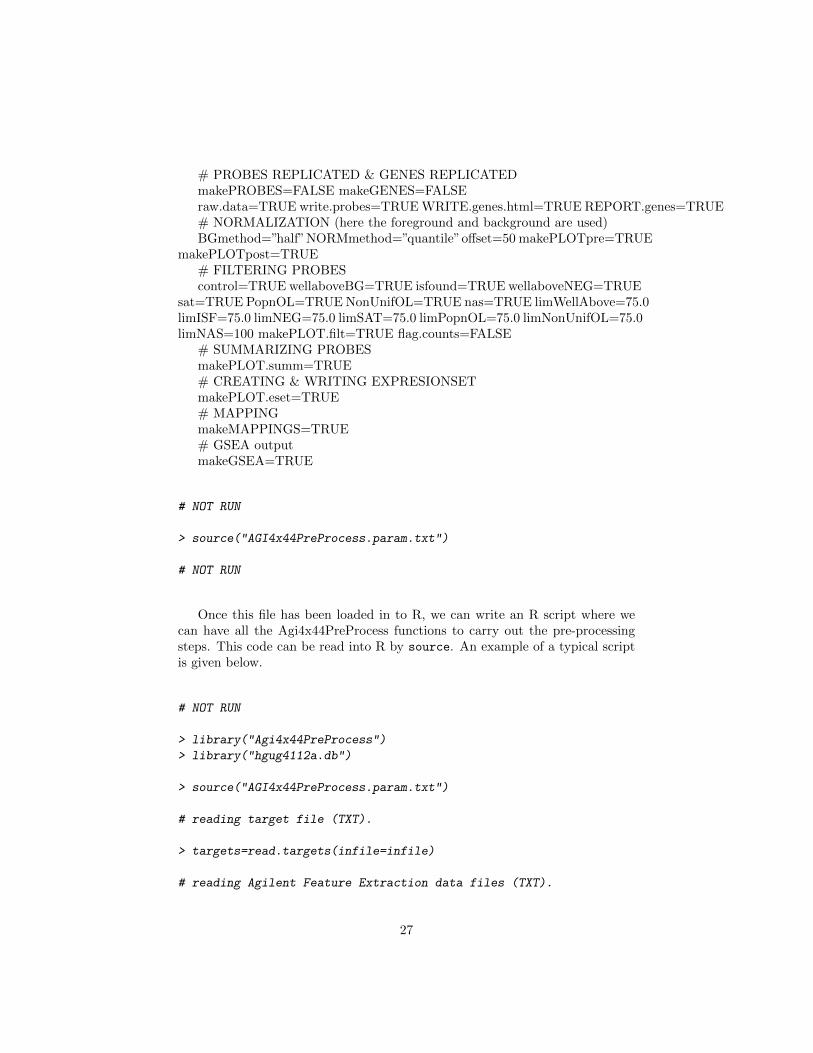
# PROBES REPLICATED & GENES REPLICATEDmakePROBES=FALSE makeGENES=FALSEraw.data=TRUE write.probes=TRUE WRITE.genes.html=TRUE REPORT.genes=TRUE# NORMALIZATION (here the foreground and background are used)BGmethod=”half”NORMmethod=”quantile”offset=50 makePLOTpre=TRUE
makePLOTpost=TRUE# FILTERING PROBEScontrol=TRUE wellaboveBG=TRUE isfound=TRUE wellaboveNEG=TRUE
sat=TRUE PopnOL=TRUE NonUnifOL=TRUE nas=TRUE limWellAbove=75.0limISF=75.0 limNEG=75.0 limSAT=75.0 limPopnOL=75.0 limNonUnifOL=75.0limNAS=100 makePLOT.filt=TRUE flag.counts=FALSE
# SUMMARIZING PROBESmakePLOT.summ=TRUE# CREATING & WRITING EXPRESIONSETmakePLOT.eset=TRUE# MAPPINGmakeMAPPINGS=TRUE# GSEA outputmakeGSEA=TRUE
# NOT RUN
> source("AGI4x44PreProcess.param.txt")
# NOT RUN
Once this file has been loaded in to R, we can write an R script where wecan have all the Agi4x44PreProcess functions to carry out the pre-processingsteps. This code can be read into R by source. An example of a typical scriptis given below.
# NOT RUN
> library("Agi4x44PreProcess")
> library("hgug4112a.db")
> source("AGI4x44PreProcess.param.txt")
# reading target file (TXT).
> targets=read.targets(infile=infile)
# reading Agilent Feature Extraction data files (TXT).
27
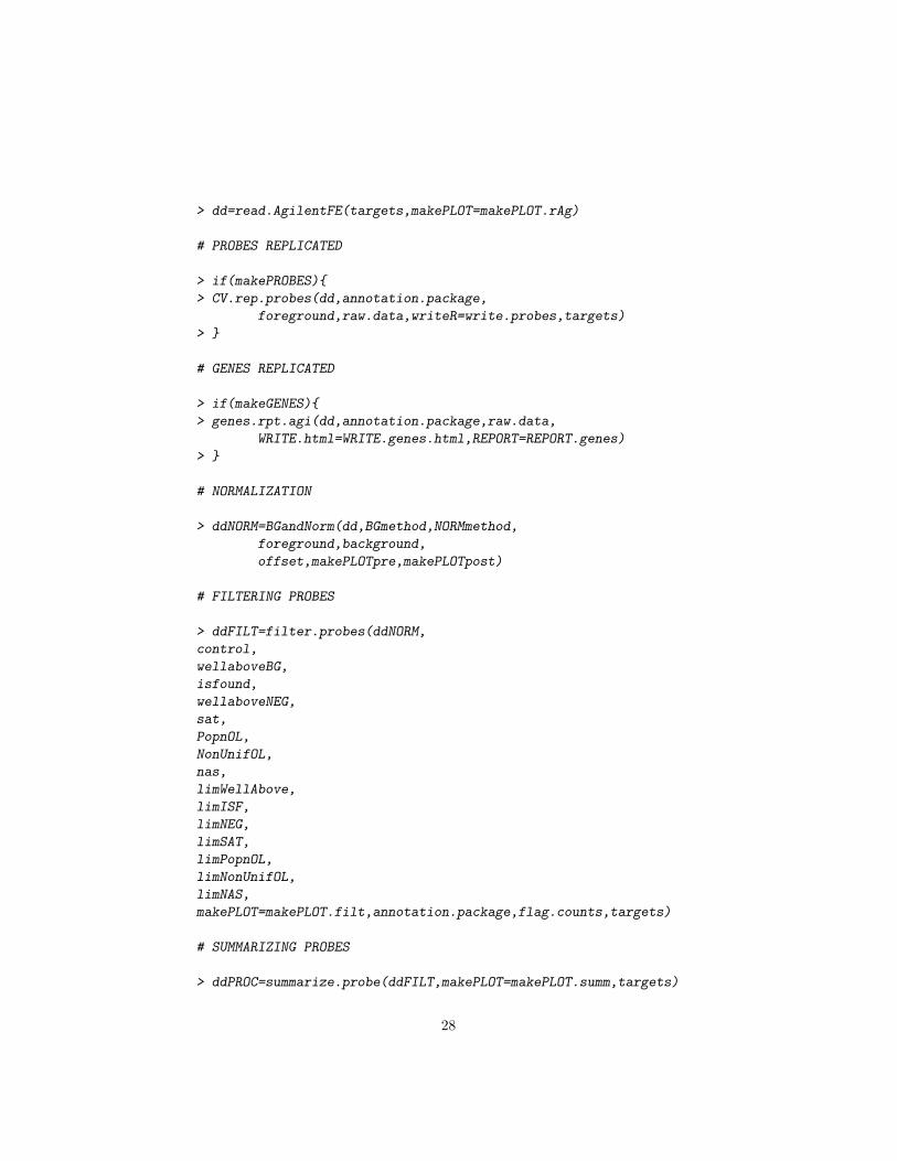
> dd=read.AgilentFE(targets,makePLOT=makePLOT.rAg)
# PROBES REPLICATED
> if(makePROBES){
> CV.rep.probes(dd,annotation.package,
foreground,raw.data,writeR=write.probes,targets)
> }
# GENES REPLICATED
> if(makeGENES){
> genes.rpt.agi(dd,annotation.package,raw.data,
WRITE.html=WRITE.genes.html,REPORT=REPORT.genes)
> }
# NORMALIZATION
> ddNORM=BGandNorm(dd,BGmethod,NORMmethod,
foreground,background,
offset,makePLOTpre,makePLOTpost)
# FILTERING PROBES
> ddFILT=filter.probes(ddNORM,
control,
wellaboveBG,
isfound,
wellaboveNEG,
sat,
PopnOL,
NonUnifOL,
nas,
limWellAbove,
limISF,
limNEG,
limSAT,
limPopnOL,
limNonUnifOL,
limNAS,
makePLOT=makePLOT.filt,annotation.package,flag.counts,targets)
# SUMMARIZING PROBES
> ddPROC=summarize.probe(ddFILT,makePLOT=makePLOT.summ,targets)
28

# CREATING EXPRESIONSET OBJECT
> esetPROC=build.eset(ddPROC,targets,makePLOT=makePLOT.eset,
annotation.package)
# WRITING EXPRESIONSET OBJECT: ProcessedData.txt
> write.eset(esetPROC,ddPROC,annotation.package,targets)
# MAPPING
> if(makeMAPPINGS){
> mappings=build.mappings(esetPROC,annotation.package)
> }
# GSEA OUTPUTS
> if(makeGSEA){
> gsea.files(esetPROC,targets,annotation.package)
> }
# NOT RUN
References
[1] Agilent. Agilent Feature Extraction Reference Guide, 2007.
[2] B. Bolstad, F. Collin, J. Brettschneider, K. Simpson, L. Cope, R. Irizarry,and T.P. Speed. Quality Assesement of Affymetrix GeneChip Data, pages397–420. Springer, New York, 2005.
[3] R Development Core Team. R: A language and environment for statisticalcomputing. R Foundation for Statistical Computing, Vienna, Austria, 2005.ISBN 3-900051-07-0.
[4] Gordon K Smyth. Limma: linear models for microarray data, pages 397–420.Springer, New York, 2005.
[5] Aravind Subramanian, Pablo Tamayo, Vamsi K Mootha, Sayan Mukherjee,Benjamin L Ebert, Michael A Gillette, Amanda Paulovich, Scott L Pomeroy,Todd R Golub, Eric S Lander, and Jill P Mesirov. Gene set enrichment anal-ysis: a knowledge-based approach for interpreting genome-wide expressionprofiles. Proc Natl Acad Sci U S A, 102(43):15545–15550, Oct 2005.
29


