AFIT/GOR/ENS/93M- 18

AD-A262 492 DT""S... •I•ELECTE

APR 5 190C

BRADLEY FIGHTING VEHICLE GUNNERY:An Analysis of Engagement Strategies

for the M242 25-mm Automatic Gun

THESIS

James G. RileyCaptain, USA

AFIT/GOR/ENS/9 3M- 18

Reproduced FromBest Available Copy

Approved for public release; distribution unlimited

93-07016.93 4 02 1 A.1 I;l lEiim _

;. 4 000/10 o6/73

THESIS APPROVAL

STUDENT: Captain James G. Riley CLASS: GOR 93-M

THESIS TITLE: BRADLEY FIGHTING VEHICLE GUNNERY: AnAnalysis of Engagement Strategies for the M242 25-mmAutomatic Gun

DEFENSE DATE: 26 FEB 93

COMMITTEE: NAME/DEPARTMENT SIGNATURE

Co-Advisor Lt Col Kenneth W. Bauer/EN

Co-Advisor Prof. Daniel E. Reynolds/ENC

AcCesion For

NTIs CRA&.

/n UnbutincLd 0

ByDIIiu~n

A11,daIbii~ty Codes

Avdif ;dlidor

D is Spectai

AFIT/GOR/ENS/93M-18

BRADLZY FIGHTING VEHICLE GUNNERY:An Analysis of Engagement Strategies

for the M242 25-mm Automatic Gun

THESIS

Presented to the Faculty of the School of Engineering

of the Air Force Institute of Technology

Air University

In Partial Fulfillment of the

Requirements for the Degree of

Master of Science in Operations Research

James G. Riley, B.S.

Captain, USA

March 1993

Approved for public release; distribution unlimited

Preface

The purpose of this research was to improve Bradley

Gunnery procedures. The study of engagement strategies was

undertaken to provide additional guidance for the structure

of the 25-mm point target engagement.

A model, based on established US Army Material Systems

Analysis Activity (AMSAA) methodology, was used to simulate

the gunnery process and provide data output in order to

analyze various strategies and procedures. Although limited

to the single stationary BMP-type target engagement, the

results of the analysis provide definite insight into the

structure of an efficient and effective 25-mm engagement.

I wish to credit COL John T.D. Casey with the

inspiration for this study. A true student of the Bradley

and gunnery in particular, COL Casey taught me to question,

analyze, and improve the methods and tools of our chosen

profession. I would also like to thank Mr. Ken Hilton and

Donna Quirido of AMSAA for their invaluable technical

assistance in the development of this thesis. My thesis

committee, LTC Kenneth Bauer and Prof. Dan Reynolds deserve

special thanks for guiding me through the thesis ordeal and

keeping an open mind when exposed to "Army stuff." Lastly,

I am forever indebted to my wife Kathy and two sons,

Jonathan and Scott, for their patience, understanding and

constant support.

James G. Riley

ii.

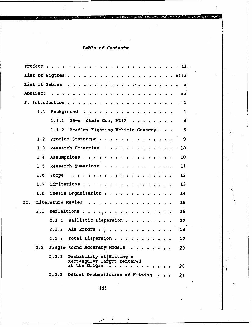
rable of Contents

Preface . . . . . . . . . . . . . . . . . . . . . . . ii

List of Figures . . . . . . . . . . . . . . . . . . . . viii

List of Tables .. . . . . . . . . .x

Abstract . . . . . . . . . . . . .. . . . . . . xi

I. Introduction . . . . . . . . . . 1

1.1 Background . . . . . . . .... 1

1.1.1 25-mm Chain Gun, M242 ........ 4

1.1.2 Bradley Fighting Vehicle Gunnery . . . 5

1.2 Problem Statement. .............. 9

1.3 Research Objective 10

1.4 Assumptions . . . e o 10

1.5 Research Questions . . . . . . . . . . o 11

1.6 Scope . . . . . . . . . . . . . . . . . 12

1.7 Limitations . . .. . . . . . ... .. . 13

1.8 Thesis Organization . . . . . . . . . . . . . 14

II. Literature Review o o o .. . . . . . . . . . . 15

2 . 1 D e f i n i t i o n s . . . \ .0 ' * . * * . * . . . 1 6

2.1.1 Ballistic Dispersion . .. . . . 17

2.1.2 Aim Errors \............. 18

2.1.3 Total Dispers on ... 1.. ... 9

2.2 Single Round Accuracy Models . . . . . . . . 20

2.2.1 Probability of Hitting aRectangular Ta get Centeredtthe Origin .. . . . . . 20at th r g n . . . . . . . . . . . ... 0

2.2.2 Offset Probabilities of Hitting . . . 21

iii

- /

2.2.3 Approximation Methods . . . . . . . . 22

2.2.3.1 Polya-Williams . . . . . . . . 22

2.2.3.2 von Neumann-Carlton DiffuseTarget Concept . . . . . . . . 22

2.3 Multiple Round Hit Probabilities . . . . . . 24

2.3.1 The Diffuse-Target ApproximationMethod 24

2.3.2 Markov Dependent Rounds Model . . . . 26

2.3.3 Simulation methods. . . . . . . . . . 27

2.4 Conclusion . . . . . ... . 31

III. Model Formulation . . . . . . . . . . . . . . . . 32

3.1 Introduction ................. 32

3.2 Simulat-.on Methods . . . . . . . . . . . . . 33

3.3 Simulation Model POINT TARGET ENGAGEMENT . . 34

3.3.1 Main Program... .... . .... . 34

3.3.2 Sensing Rounds and Bursts . . . . . . 35

3.3.3 Range-in . . . . . . . . . . 36

3.3.4 KillingBursts............ 37

3.3.5 Fire for Effect ........... 38

3.4 A Methodology for Estimating Quasi-Combat Dispersions for AutomaticWeapons 39

3.4.1 Development Test (DT) Digpersions . . 39

3.4.2 First Round Hit Probability . . . . . 40

3.5 Point Target Engagement Simulation ModelDocumentation # 43

3.5.1 Engagement Strategy . . . . . 45

3.5.2 Target Characteristics . . . . . . . . 45

3.5.3 Statistical Counters . . . . . . . . . 48

iv

N

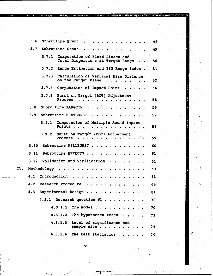
3.6 Subroutine Event .. . ......... 48

.3.7 Subroutine Sense .. ....... ... . 49

3.7.1 Computation of Fixed Biases andTotal Dispersions at Target Range . . 50

3.7.2 Range Estimation and ISU Range Index . 513.7.3 Calculation of Vertical Miss Distance

on the Target Plane .... . . .. 52

3.7.4 Computation of Impact Point ..... 54

3.7.5 Burst on Target (BOT) AdjustmentProcess . . . 55

3.8 SubroutineRANGEIN ............. 6

3.9 Subroutine FRSTBURST ............ 57

3.9.1 Computation of Multiple Round ImpactPoints . . . . . . . . . . . . . . . . 58

3.9.2 Burst on Target (BOT) AdjustmentProcess . . . . . . . . . . . . . . 59

3.10 Subroutine KILLBURST . . ....... . . . 60

3.11 Subroutine EFFECTS .............. 61

3.12 Validation and Verification • • • ..... 61

IV, Methodology . . . . 63

4.1 Introduction 63

4.2 Research Procedure . ............ 63

4.3 Experimental Design . 64

4.3.1 Research question #1 .......... 70

4.3.1.1 The model ........... 70

4.3.1.2 The hypotheses tests ..... 73

4.3.1.3 Level of significance andsample size ......... 74

4.3.1.4 The test statistics ...... 74

v

4.3.1.5 Multiple Comparisons . . . . . 75

4.3.2 Research Question #2 . . . . . . . . . 76

4.3.2.1. The model . . . . . . . . . . 76

4.3.2.2 The hypotheses test . . . . . . 77

4.3.2.3 Level of significance andsample size. .. . ... . .. 77

4.3.2.4 The test statistic . . . . . . 77

4.3.2.5 Multiple Comparisons . . . . . 78

4.3.3 Model Adequacy .... .... 78

V. RESULTS . . . . . . . . .. . . . .. . . . . . . . . . 80

5.1 Research Questionl .. ..1. . 80

5.1.1 Influence of YAKIMA Aim PointAdjustment Algorithm ... . . . . . .. 81

5.1.2 Firing Mode Influences . . . . . . . . 86

5.1.3 Influence of Engagement Strategies . . 87

5.2 Research Questionl12 . .. .0. .. . . .. 88

5.3 Model Adequacy . . . . . . . . . . . . . . . 88

V1. CONCLUSIONS AND RECOMMENDATIONS . . . . . . . . . 90

6.1 Engagement Strat teyg. . ..... 90

6.2 Battlesight Versus Precision Gunnery . . . . 94

6.3 Fire for Effect Bursts . . . . . . . . . . . 97

6.4 Recommendations for Further Study . . . . . . 99

Appendix A: Simulation Model Flowcharts . . . . . . . 100

Appendix B: POINT TARGET ENGAGEMENT Simulation ModelComputer Code . . . . o . . . . . . . . . 114

Appendix C: Fixed Bias and Rando.-i DispersionRegression Equations . . . . . . . . . . . 130

Appendix D: Analysis of Shotgun Model A~swt~ption . 136

vi

Bibliography .. . . . . . . . . . . . . . . . . . . . 140

vii

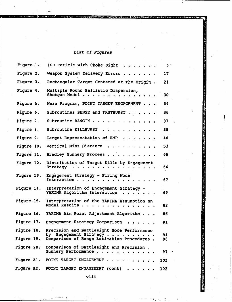
List cf Figures

Figure 1. ISU Reticle with Choke Sight . . . . . . . 6

Figure 2. Weapon System Delivery Errors . . . . . . . 17

Figure 3. Rectangular Target Centered at the Origin . 21

Figure 4. Multiple Round Ballistic Dispersion,Shotgun Model ...... ......... 30

Figure 5. Main Program, POINT TARGET ENGAGEMENT . . . 34

Figure 6. Subroutines SENSE and FRSTBURST . . . . .. 36

Figure 7. Subroutine RANGIN . ........ .... 37

Figure 8. Subroutine KILLBURST . . . . . ... . . . . 38

Figure 9. Target Representation of BMP . . . . ... 46

Figure 10. Vertical Miss Distance . . . . . . . . . . 53

Figure 11. Bradley Gunnery Process . ... . . . . . . . 65

Figure 12. Distribution of Target Kills by EngagementStrategy . . . . . . . . . . . . . . . . . 66

Figure 13. Engagement Strategy - Firing ModeInteraction n . ...... 67

Figure 14. Interpretation of Engagement Strategy -

YAKIMA Algorithm Interaction . . . . . . . 69

Figure 15. Interpretation of the YAKIMA Assumption onModel Results...... . . . . . . . . . 82

Figure 16. YAKIMA Aim Point Adjustment Algorithm . . . 86

Figure 17. Engagement Strategy Comparison . . . . . . 91

Figure 18. Precision and Battlesight Mode Performanceby Engagement Strategy . . . . . . . . . . 94

Figure 19. Comparison of Range Estimation Procedures . 96Figure 20. Comparison of Battlesight and Precision

Gunnery Performance . ........... 97

Figure Al. POINT TARGET ENGAGEMENT . . . . . . . . . . 101

Figure A2. POINT TARGET ENGAGEMENT (cont) . . . . . . 102

viii

S. .... _-

Figure A3. Subroutine EVENT . . . . . . . . . . 103

Figure A4. Subroutine EVENT (cont) . . . . . . . . . . 104

Figure A5.* Subroutine EVENT (cont) . . . . . . . . . . 105

Figure A6. Subroutine SENSE . . . ... . . . . . . . . 106

Figure A7. Subroutine SENSE (cont) . . . ....... 107

Figure A8. Subroutine RANGIN ............. 108

Figure A9. Subroutine FRSTBURST ........... 109

Figure A10. Subroutine FRSTBURST (cont) . .o. . . . o 110

Figure All. Subroutine FRSTBURST (cont) . o . o .. . 111

Figure A12. Subroutine KILLBURST ...... . . .. 112

Figure A13. Subroutine KILLBURST (cont) ....... 113

Figure C1. Scatter Plot of Fixed Bias Data ...... 132

Figure C2. Scatter Plot of Total Dispersion Data ... 134

Figure D1. Time Series Plot of Vertical Axis ImpactCoordinates . . . . . .. . . . . .. . . . 138

Figure D2. Time Series Plot of Horizontal Axis ImpactCoordinates . . . . . . 139

ix

List of Tables

Table 1 First Round Hit Probability -

M791 APDS Ammunition 25-mm M242 Gunversus 2.3 x 2.3 Meter Target ..... 29

Table 2 25-mm DT Dispersion Estimates . . . . . 40

Table 3 Input Values to PHI for 25-mm APDS-TM791 Round Fired From M242 Gun Mountedon SFVS . . . . . . . . . . . . . . . . 42

Table 4 Target Attributes ........... 45

Table 5 Visible Width (m) of a BMP Oriented at VariedAngles . . . . . . . . . . . . . . . . . 47

Table 6 RESULTS FROM PHi Fixed Biases and TotalDispersions . . . . . . . . . . . . . . 50

Table 7 Cumulative Range-in Probabilities andAverage Niumber of Range-in Rounds . . . 85

Table 8 Tukey's Studentized Range (HSD) Test . . 87

Table 9 Target Hits by Burst Length . . . . . . 88

x

Abstract

This thesis studies various engagement strategies for

the Bradley Fighting Vehicle's 25-mm automatic gun firing

APDS-T ammunition against a BMP-type target. The Army

currently provides only the broadest guidance for the

structure of the 25-mm point target engagement which results

in the employment of an assortment of strategies throughout

the Bradley community. The goal of this research was to

determine if a best method exists.

Bradley gur-^-y is a complex set commander/gunner

interactions which can be difficult to represent with the

analytic models commonly found in the literature. A model,

based on the simulation methods used by the US Army Material

Systems Analysis Activity (AMSAA), was developed to simulate

the gunnery process in order to analyze the effects of

firing a set pattern of single sensing rounds and multiple

round bursts for the purpose of 'killing' the target.

Analysis of variance techniques were used to

characterize the effects of engagement strategies, precision

and battlesight firing modes, and the burst on target (BOT)

direct fire adjustment technique on the simulated Bradley

gunnery process. Based on these results, conclusions and

recommendations concerning the structure of the 25-mm point

target engagement are discussed.

Ix

BRADLEY FIGHTING VEHICLE GUNNERY

AN ANALYSIS OF ENGAGEMENT STRATEGIZES FOR THE 25-MM GUN

Z. Introduction

1.1 Background

New technology and doctrinal concepts have changed the

face of the Army. Our senior planners envision that the

nature of modern warfare will lead to future battles of

unprecedented scope and intensity. To meet this challenge

the Army identifies three essential components to superior

performance in combat: superb soldiers and leaders; a sound

doctrine for fighting; and the finest weapons and supporting

equipment available.

First and foremost, well trained and well led soldiers

are the key to victory in future battles just as they have

been in the past. The Army places a premium on recruiting

quality soldiers and providing the most realistic and

demanding training available.

To tell their soldiers 'how to fight', the Army has

developed AirLand Battle Doctrine. As described in Field

Manual (FM) 100-5, AirLand Battle "reflects the structure of

modern warfare, the dynamics of combat power, and the

application of the classical principles of war to

contemporary battlefield requirements" (7:9). A key aspect

of this doctrine is its focus on combined arms operations;

the coordinated use of Armor, Infantry, Field Artillery,

Army Aviation, and Air Force Close Air Support (CAS) to

1

/

maximize the tremendous lethality of numerous weapon systems

and destroy the enemy.

To provide the best weapons and equipment for American

soldiers to fight with on the modern battlefield, the Army

has developed new systems for eech of the major combat arms:

the Ml Abrams main battle tank; the AH-64 Apache attack

helicopter; the multiple launch rocket system (MLRS); and,

the subject of this research, the M2 Bradley infantry

vehicle. (7:5-7)

The Bradley Fighting Vehicle (BFV) is a fully-track d

armored combat vehicle armed with two Tube-launched,

Optical-tracked, Wire-guided (TOW) anti-tank missile

launchers, a 25-mm bushmaster chaingun, and a 7.62mm coax

machine gun. It is also capable of carrying a six man

infantry squad inside. As a weapons platform, the Bradley

can engage and destroy all known armor threats out to 3750

meters using the TOW missile. The 25-mm chaingun can fire

two types of ammunition: armor piercing discarding sabo

(APDS) with an effective range of 1700 meters and

high-explosive incendiary (HEI-T) with an effective range of

3000 meters, allowing it to engage lightly armored vehicles,

unarmored vehicles, or suppress crew served weapons

positions. The coax machine gun has an effective range of

900 meters and can be used to engage dismounted infantry or

suppress crew served weapons positions. As a personnel

carrier, the Bradley provides excellent protection for the

2

infantry squad from indirect and small arms fire. The squad

can also quickly dismount to perform traditional infantry

missions.

The Bradley was originally designed as the replacement

for the M113 family of armored personnel carriers which were

the primary means of transportation for infantry personnel

assigned to heavy divisions during the late 60s and the 70s.

Two events changed the original concept.

In 1967, the Soviets fielded the BMP (Bronevaya

Maschina Piekhota); a fully tracked armored amphibious

infantry combat vehicle with a turret mounted 73mm

smoothbore gun and a 7.62mm coax machine gun. Additionally,

a turret mounted launching rail for the SAGGER anti-tank

guided missile provided the BMP with the capability to

effectively engage tanks out to 3000 meters. It also had a

troop compartment for eight infantrymen complete with firing

ports which allowed them to fire their assault rifles from

inside. The BMP represented a transition from the 'armored

- personnel carrier' to the 'infantry combat vehicle' in the

Soviet and most Warsaw Pact armies. The Soviets appeared to

have a revolutionary new capability to wage rapid combined

arms offensive operations with tanks, self-propelled

artillery, and the BMP. The second event was the 1973 Yom

Kippur War. During the war, anti-tank guided missiles

(ATGM) proved to be extremely effective tank killers at

ranges beyond 3000 meters. In an effort to offset the

3

I

perceived Soviet advantage with the BMP and capitalize on

existing ATGM tachnology, the Bradley design was altered to

incorporate the TOW missile system and create an effective

match for the BMP. The original one-man turret design gave

way to a two-man version to allow the mounting of a twin TOW

launcher. The sophisticated sighting system for the TOW was

integrated, which also greatly enhanced the engagement

capabilities of the 25-mm gun. The troop compartment shrank

as a result, thereby cutting the number of infantrymen from

eleven to six. It was generally believed, however, that the

improved firepower of the new configuration was an

acceptable tradeoff. (9:185-201)

1.1.1 25-mm Chain Gun, 1242. The main armament of the

Bradley Fighting Vehicle (BFV) is a 25-mm, fully automatic,

externally powered bushmaster chain gun. It is used to

destroy lightly armored vehicles: specifically the BMP

(5:1_2). The gun is capable of firing two types of

ammunition; armor-piercing discarding sabot with tracer

(APDS-T) and high-explosive incendiary with tracer (HEI-T).

APDS-T is the appropriate ammunition for engagements against

the BMP. At one time, it was commonly believed that six

APDS-T rounds impacting on a BMP would render it combat

ineffective. In addition to these six rounds, two

additional sensing rounds were allocated for a total of

eight rounds per single engagement. For training purposes,

the same number of rounds (8) are allocated for each

4

I' ,/

engagement; however, the number of hits required to simulate

a 'kill, is reduced to three rounds (4:10_47). The 25-mm is

also capable of three rates of fire: (1) single shot - as

fast as the Bradley Commander or gunner can pull the

trigger, (2) low rate - 100 rounds per minute, plus or minus

25 rounds, and (3) high rate - 200 rounds per minute, plus

or minus 25 rounds. In the broadest terms, an engagement

strategy is a specific combination of single shots and/or

multiple round bursts totaling eight, fired at a particular

rate in order to destroy an identified target.

The sighting and weapons control component for the

25-mm gun is the Integrated Sight Unit (ISU).

The gunner and commander use the integrated sight unitto locate, identify, range and engage targets day andnight. The ISU is moved with the turret in azimuth andfollows weapons elevation by means of a servo drivenmirror that is electrically linked to the selectedweapon's rotor movement. ... In gun mode, the mirrorfollows the gun rotor elevation/depression. 25-mmboresight adjustments in elevation movea the mirror toalign with the 25-mm. Azimuth adjustment moves theaiming reticle ... The sighting mirror is furtheradjusted for superelevation by dialing in estimatedrange. (Superelevation is used to maintain weaponaccuracy by adjusting the mirror line-of-sight inelevation to allow for trajectory of the selectedammunition.) ... The gunner's estimate of range isdialed into the sight which lowers the weapon torealign on target. Superelevation is stepped in 200meter increments and is displayed in the gunner's andcommander's eyepieces ... (8:44).

1.1.2 Bradley Fighting Vehicle Gunnery.

Unfortunately, range to the target must be visually

estimated. The Bradley gunner's or commander's ability to

accurately determine the range to a target is dependent on

5

the tactical situation. In a defensive scenario several

passive range determining methods can greatly increase the

crews capability. Target reference points, at known

distances within an established sector of fire, allow the

crew to quickly and accurately range the target. The

reticle within the ISU also has a horizontal ranging stadia

(choke sight) which can be used to determine the range to

BMP type vehicles. The stadia lines are horizontally spaced

to represent the visual size of a 1.8 meter high vehicle at

various ranges from 500 to 3000 meters. Figure 1.

RETICLE

LEADLINES SGTCHOKE"

SIGH

AMMO

INDEX SELECTED

RANGE

Figure 1. ISU Reticle with Choke Sight

6/

- ~ I .-.-----

A final method makes use of the relationship between

the reticle in standard military binoculars and the mil unit

of angular measurement. A quick reference table with

various mil and range relationships is commonly used by

Bradley commanders~ to determine the range to a vehicle

target identified with binoculars. The principal drawback

to these methods is the amount of time required to apply

them. Because defensive operations usually provide a higher

degree of concealment and protection from enemy fir e, the

time is usually available. FM 23-1, Bradley Fighting

Vehicle Gunnery, specifically limits the use of these

methods to the defense (4:3_17-3_21). Offensive operations

are entirely different: time is absolutely critical!

FM 23-1 also defines two types of fire commands which

reflect either a defensive or offensive engagement:-

precision and battle sight.

Precision fire is the most accurate type of directf ire. Precision gunnery techniques should be used onlywhen time permits, such as when the (Bradley) vehicleis in a defensive position or in an overwatch position...once a target is acquired, the Bradley commander

issues a precision fire command. Once the gunner orBradley commander has identified the target, he rangesto the target as accurately as possible and announcesthat range. ... Battle sight is a gunnery techniquethat can be used in a most-dangerous surprisesituation. it is not as accurate as precision gunnerytechniques; but battle sight gunnery is the quickestway to engage the enemy before he can fire. (4:4_5)

Battles ight is a planned engagement that assumes the

most likely threat is the BMP and the most likely range to

that threat will be 1200 meters. The first assumption is

7

obvious. The second attempts to make the best use of the

.ballistic characteristics of the APDS-T round. The ISU and

the gun are zeroed to this range to give the highest

probability of a first round hit. Zeroing procedures adjust

the ISU reticle to establish a definite relationship betw een

the trajectory of a particular round and the line of sight

to the target at a specific range (4:2_1). The range

assumption leaves a large opportunity for error between the

'actual range to a threat target and 1200 meters. if the

crew is able to determine that the range to the identified

target exceeds 1400 meters, FM 23-1 recom~mends that the

gunner index 1600 meters (extended battlesight) to increase

the probability of a first round hit. The nature of the

future battlefield may be the limiting factor on the crew's

ability to do so.

Bradley platoons must be prepared to move and torapidly engage .multiple targets. Platoons will beoperating within irregular battle lines. Depending onthe tactical situation and the area of operations,Threat targets will be intermixed with friendly andneutral (civilian) vehicles. ... Survival depends on

---the platoon's ability to search for, acquire, classify,confirm, and rapidly engage Threat targets. Bradleyplatoons must take advantage of the situation and firefirst. (5:3_1)

This type of 'pressure packed' environment creates some

doubt as to whether even this minimal amount of range

estimation will take place. Although ranging errors can

also creep into a defensive engagement, they would logically

be much smaller as long as one of the various range

determination methods is used. To correct for these

8

\/

inherent ranging errors a direct fire adjustment technique

called burst on target is most often used.

Burst on target (BOT) uses the observed impact of the

rounds from a combination of single shots (sensing rounds)

and multiple shots (killing bursts) to guide the strike of

the round onto the target. If the first round fired at a

target fails to hit it, the gunner and vehicle commander,

observe where the round strikes in relation to the target

and convert the relationship into an executable correction

for the original point of aim. Corrections are normally

given relative to the size of the target; "up 1/2 target

form, right one target form", etc. The adjustment procedure

is repeated until a round impacts on the target, at which

time the verbal correction is replaced by the command

"target". This command directs the gunner to continue to

engage the target with 3!-5 round bursts until it is

destroyed or the command "cease fire" is given. Fach of

these killing bursts are also observed and corrected as

necessary (4:4_19).

1.2 Problem Statement

FM 23-1 currently provides only the broadest guidance

for the structure of the 25-mm point target engagement.

"The gunner fires a sensing round, announces his observation

and adjusts rounds by BOT. The gunner then fires a three to

five-round burst on the target. He continues firing bursts

9

-- , - i -

until the target is destroyed or the command CEASE FIRE is

given (4:4_12)." Consequently, every Bradley unit has

developed it's own 'engagement strategy': a specific

combination of single shots and/or multiple round bursts

totaling eight, fired at a particular rate in order to

destroy an identified target. The effectiveness of possible

engagement strategies and those currently in use throughout

the Army may vary significantly and should be evaluated.

1.3 Research Objective

The purpose of this research is to identify the best

engagement strategy for the 25-mm gun, if one exists, so

that Bradley gunners will become more efficient at engaging

and destroying threat targets.

1.4 Assumptions

The underlying assumption of the Bradley 25-zri point

target engagement is that eight rounds is the appropriate

number required to kill a single BMP. The Army Material

Systems Analysis Activity (AMSAA) is currently quoted as the

source for this estimate of eight rounds per BMP target.

According to analyst Donna Quirido, AMSAA does not provide

or support any such estimate (30). The true source of this

estimate is currently unknown.

Despite the questionable validity of the eight rounds

to kill a BMP estimate, this number will be the assumed

10

.*"- ." - • ,\ i ; - I

length, in rounds fired, of a point target engagement.

Bradley gunnery training and evaluation outlined in FM 23-1

revolves around this number. Until this estimate is

officially modified, any analysis of engagement strategies

must reflect this current 'truth.' Operationally, the crew

will undoubtedly continue to fire at the target until the

desired effect is achieved. FM 23-1 states that "the

minimum standard is to achieve a mobility or firepower kill.

the Threat vehicle can no longer move under its own

power. .. (or) can no longer use its weapon systems"

(5:4_32). It is assumed that a gunner will 'expand' the

initial eight round engagement with repeated multiple round

bursts of equal length until the desired target effect is

obtained.

1.5 Research Questions

Based on the assumptions noted above, the research will

focus on answering the following questions: 1. What is the

best engagement strategy for the Bv'V 25-mm firing APDS-T

ammunition at a EMP type point target? 2. What is the most

efficient burst size for expanding the initial engagement

strategy to achieve the desired target effect? The first

question deals with the first eight rounds fired at the

target, either in training or in real battle. The second

question addresses the operational environment, where kill

effect on an actual armored vehicle determines the end of

the engagement. The answer to these questions will provide

additional training guidance to Bradley units as they

prepare for their wartime missions during gunnery exercises.

1.6 Scope

This research will focus on the point target engagement

using the M791 APDS-T round. The newer M919

armor-piercing, fin stabilized discarding sabot with tracer

round (APFSDS-T) lacks sufficient live-fire testing to be

included in this analysis. The increased muzzle velocity

and maximum effective range (classified) of the 919 round

may produce significantly different results or merely extend

the target range considerations. Based on unclassified

information about the new round in Armed Forces Journal

International;

Ballistically identical to the M791 ... , the M919allows -he Bradley to defeat thicker armor at greaterrange than previous rounds. (As a result of) ...improved depleted uranium (DU) penetrator andpropellant technologies for the round. (19:22)

the latter assumption appears to be the case.

The M792 HEI-T round will not be considered. The

round-to-round random dispersion of the HEI-T is

significantly greater than that of APDS-T which would

presumably lead to significantly different results

(2:11-12). Since HEI-T is predominately used for

suppression, no attempt will be made to determine an overall

best engagement strategy for both types of ammunition.

12

Every effort will be made to consider all feasible

engagement strategies. A letter submitted to the January-

February issue of INFANTRY magazine requested input from the

Bradley community so that no engagement strategy currently

in use will be inadvertently ov3rlooked (32:1).

Based on the assumption regarding additional killing

bursts fired after the initial eight Lounds to achieve a

desired target effect, the research will include an analysis

of three, four, and five round burst patterns to determine

if the length of burst is significant. Bursts of more than

five rourds will not be evaluated based on readily available

ea(uunition considerations.

1.7 Limitations

The model used in this research will simulate the 25-mm

point target engagement of a stationary Bradley Fighting

Vehicle against a BMP sized stationary target only. With

its fully stabilized gun, the Bradley is certainly capable

of effectively engaging targets while ctationary and on the

move. Threat vehicles will also be either stationary or

moving on the battlefield creating :"merous stati~nary-on-

moving and moving-on-moving types of engagements. However,

the single scenario used in this research should p ovide an

indication as to whether the use of a particular er gagement

strategy might be advantageous. The enumerable combinations

of moving and stationary aspects could then be simulated,

13

N

perhaps in the Unit Conduct of Fire Trainer (UCOFT)

environmerit, to determine if the use of a set engagement

strategy remains feasible and/or warranted.

1.8 Thesis Organization

Chapter 2 is a literature review that summarizes

pertinent information about weapon systems modeling and

simulation. Chapter 3 discusses formulation of the

simulation model. It also provides detailed documentation

of the simulation and discussion of the algorithms used to

model the 25-mm engagement process. Chapter 4 reviews the

research methodology and evaluation of model results.

Chapter 5 presents the analysis and findings from the model

output. Lastly, Chapter 6 concludes the thesis and presents

recommendations for further study.

14

N o .

II. Literature Review

The purpose of this literature review is to research

weapon systems modeling techniques in order to develop a

detailed and accurate model representation of the 25-mm gun

system. This model will be the analytic tool used to

compare and eventually rank various engagement strategies.

Obviously, conclusions drawn from an invalid model would be

of no use to the Army. Bradley gunnery techniques were

described in Chapter 1. The discussion covered the topic

only to the level necessary to understand how the vehicle

crew functions during an engagement. The technical aspects

of the 25-mm gun system were also addressed in detail

sufficient to outline the key functions to be modeled and

how the gun/sighting system works. The modeling methods for

the various factors represented in the Bradley gun Isystem

will be outlined without extensive historic or theoretical

background. The methods presented are those generally

accepted by the Army Material Development and Readiness

Command, summarized in DARCOM Pamphlet 706-101, and should

therefore not require a more rigorous theoretical

justification (6). The review is divided into three major

parts: definitions, single round accuracy modeling, and

multiple round accuracy modeling. The first section will

define the various terms and concepts involved in weapon

systems modeling and ballistics. The second section will

15

focus on basic models that determine whether a single round

fired will hit the target, while the last section will

address models for engagements in which multiple rounds are

fired at a single target.

2.1 Definitions

In his Lecture Notes in High Resolution Combat

Modelling, James K. Hartman notes that

two basic principles are invoked in nearly all accuracymodels: 1. Weapon accuracy can be adequatelydescribed by considering the projectile impact point tobe a random variable. 2. The Normal probabilitydistribution is a good model for the random impactpoints. (15:7_2)

There are numerous components to the weapon delivery errors

which are described by the normal distribution. Figure 2

graphically shows the various error components of weapon

system accuracy.

Yx

S Point -

Round Impect Poin

T ,JA,tud AJ=r Po,,t(U.-)

Figure 1. Weapon System Delivery Errors

16

//-~ i '.7

2.1.1 Ballistic Dispersion. In his article, On the

Computation of Hit Probability, Hermann Josef Helgert

states,

ballistic dispersion is the combined effect ofround-to round variation in shell manufacture, powderweight, moisture content and temperature, andshort-term variations in the state of the atmosphere atthe instant of firing. In this list must be included afactor peculiar to guns mounted on unstable platformssuch as ships, namely round-to-round variations inrange and deflection caused by transitional motion ofthe gun barrel at the instant of firing, and the natureof the recoil of guns mounted on such unstable,platforms. It is commonly assumed, and there is goodsupporting experimental evidence, that ballisticdispersion is a Gaussian rakndom process with zero meanand negligible correlation between rounds. (16:670)

Ballistic Dispersions are thus defined by the relations:

Var~x Wo~ (1

Vax (y) -o, 2

2.1.2 Aim Errors. Aiming errors are errors in

determining the correct gun elevation and azimuth required

for the round fired to hit the Doctrinal Aim Point.

The Doctrinal Aim Point is the center of the visible target

area. The Actual Aim Point is the point on or near the

target where the weapon is aimed at the instant of trigger

pull. Aiming errors are the difference between the two

points. They are further categorized as systematic errors

and time varying errors. The total aim error in the

horizontal (x) and vertical (y) axes about the Doctrinal Aim

Point for the Ith shot can be expressed as:

17

u1-u(t 1 )+ u(b) (3)

v1-v(t.) + v(b,) (4)where u(b) = x component of systematic error (bias)

v(b) - y component of systematic error (bias)u(t) - x component of time variable errorv(t) = y component of time variable error

Errors in determining the range to a target or the

correct location of the visible center mass point are

systematic. Helgert states:

The net effect of the systematic errors is to imparta constant bias to the center of the impact points ofthe rounds. One's lack of knowledge of the exact valueof the constant is expressed by taking it to be asample function from another Gaussian random processwith zero mean ... (16:670)

The time varying errors in gun elevation 'and azimuth

are due to the gunner's inability to hold his aim point

steady throughout the engagement or in the case of. the

Bradley, stabilization inaccuracies. According to Helgert:

These errors give rise to aim-wander, a term thatderives from the fact that the path traced by theintersection of the gun barrel mean line of sight and aplane perpendicular to it would, as a function of time,appear to be wandering in a more or less randomfashion. The effect of the resulting sequence of aimpoints at the target is another .riearly Gaussian processwith time-varying means and auto-correlation functions.

Aim wander ... is the cause of the well knownround-to-round cýrrelation of impact points that mayexist in high-rate-of-fire guns. (16:670-571)

This time varying comI onent of aiming error, or assumptions

regarding it, are a si ificant aspect of modeling multiple\

round bursts of fire. It is assumed that ballistic

dispersion and aim errors (systematic and time varying) are

independent and also additive (16:671).

18

7 -.-

2.1.3 Total Dispersion. Based on the assumption that

the distribution of rounds is approximately Normal, the

probability density function (pdf) describes the coordinate

components of total dispersion (6:13_6):

f(X) [1/ (y-70) 1 exp [- (x-u) I/(2a)2 (5)f(Y) [I/ (V/-7Cy) ] exp[- (y-v) 2/(2a• ] V

where

u - x coordinate of Actual Aim Point

v - y coordinate of Actual Aim Point

2.2 Single Round Accuracy Models

Single round hit probability models are categorized as

either centered aim point or offset aim point in DARCOM

PAMPHLET 706-101 depending on whether aiming errors are

equal or not equal to zero. The pamphlet also presents the

models in terms of either circular or rectangular target

form. (6:141-1420) Since the BMP silhouette most closely

approximates a rectangular target, only the equations of

this form will be covered here. However, Frank E. Grubbs,

of the US Army Ballistic Research Laboratories, asserts that

the computed probability of hitting a circular target is not

significantly different from the results assuming a

rectangular target for many practical applications, *since

available vulnerability data or lethality data or other

19

input information may lead to some lack of precision anyway"

(14:58).

2.2.1 Probability of Hitting a Rectangular Target

Centered at the Origin. Figure 3 depicts a rectangular

target where the Actual Aim Point is the true center of

mass. Aiming errors are assumed to be zero.

Round Impat Point

Acatua Mmn Point Deflilanc Dispeuiaa(0.0) (CFA crOy)

Figure 2. Rectangular Target Centered at the Origin

The chance of hitting a rectangular target centered at the

origin is the product of equations (5) and (6) integrated

over their respective coordinate intervals (6:14 4).

I.,,

2.2.2 Offset Probabilities of Hittinug. Offset aim

point models take ballistic dispersion as well as systematic

aiming errors into consideration. Figure 2 depicted this

more probable engagement situation. If the coordinates of

20

the Actual Aim Point are known the hit probability model

becomes (6:14_17):

(&-)I/a, (b-$l/u

p(h)- [1/(2n)] f f exp[-tx2 +y2 )/2]dxdy (8)

Unfortunately, the aim point at trigger pull ir hardly ever

known, consequently Grubb notes that if credible aim error

estimates exist, the total aiming error expressed as

standard deviations may be included in equation (8) to

obtain a solution (14:57).

2.2.3 Approximation Methods. The probability models

presented thus far appear fairly simple, however, "the

mechenics associated with the integration are extremely

cumbersome and no closed form solution is available"

(16:673). Two of the most common approximate solution

methods are the Polya-Williams Approximation and the von

Neumann-Carlton Diffuse Target Concept.

2.2.3.1 Polya-Williams. The Polya-Williams

Approximation relates

the actual probability content of the normaldistribution to an exponential function by comparingprobabilities of hitting a square target with that of acircular target of the same area. (6:14_5)

The resulting approximation to the truncated normal

integral has a maximum relative error of 0.0075. Using

Polya-Williams, an approximate solution to equation (7) can

be calculated by (6:14_6):

where

21

p(h) [(1-exp [-2a/ X(:o~i J}-exp [-2b/ (72) )])]1/ (9)

a = half-target width

b = half-target height

2.2.3.2 von Neumann-Carlton Diffuse Target

Concept. According to the summary in DARCOM-P 706-101

(6:14_12-14_17)

the so-called 'diffuse target' concept of von Neumannand Carlton involves the use of the normal or Gaussiandistribution function over infinite limits toreplace and diffuse' the target, thereby avoidingthe complication of truncating the normal integral.consider a target, e.g., a square one, of area A on onehand and then on the other a negative squareexponential fall-off function of the Gaussian formwhich is. to I integrated over infinite limits togive the art. A. That is, the elementary area, dxdy,is weighted by such a function and then integrated. Byequating the area A of the (square target to the areafor the integral, we have

A-f jexp [- (x 2 +y 2 ) / (2k 2) 1 dxGy (10)-- -.

where k is a constant to be determined. We findimmediately that

A-21ck 2 k--/U2c (11)

Hence, the function which 'diffuses' over infinitelimits to give the desired target area A is

exp [_- (x 2 +y 2 )/A] , -ODx, y&OO (12)

This function is unity at the target center, x - y 0,and decreases to zero as the values of x, or y, orboth, increase beyond bounds. Then, for a circularnormal delivery distribution, the probability ofhitting the 'target' becomes

22

"K 4>7 79 . 7 ..... .. -.... .

p(h) -:1 (27o 2 ) f fexp [- (x 2 +y 2 ) (2k 2 )] exp [ (x 2 ÷y 2 ) / (202)] dxdy

-k 2/(k 2+a2) - A/(A+27[0 2 )(13)

It is also noted that the von Neumann-Carlton approximation

should only be used when the total delivery error is many

times larger than the target area A (6:14_17).

2.3 Multiple Round Hit Probabilities

Most of the literature concerning multiple round hit

probabilities provide results concerning the probability of

one hit given that several rounds are fired. Since the

25-mm requires three hits to destroy a target, the desired

results are: What is the probability of 1,2,..,5 hits given

that a burst of between three and five rounds is fired?

Helgert states "it is possible in principle to compute the

probability distribution of the number of hits" (16:673)

with the equation:

P (1 2 1 d f ff ... "T T

ffe f,(1" 12'"" I,) dx('i) dyi.) dx(l2) dy(i 2 )...dX(i( dyly ) (14)T

where

k = Number of rounds (1) in the burst

! - Area of the target

As before, however, there is no closed-form solution for

this equation. The three most common methods for modeling

multiple round hits involve the von Neumann-Charlton diffuse

23

I,-

target approximation, an assumption of Markov-dependence

between the rounds fired, or simulating the rounds within

the burst separately (15:9_7-9_11; 6:20_16).

2.3.1 The Diffuse-Target Approximation Method.

Multiple rounds tend to exhibit round-to-round dependencies

which must be adequately captured by the model. As noted

earlier, one of the sources of this round-to-round dependent

behavior may be the time variable aiming error. However, as

Helgert points out

if ballistic dispersion is much larger than the time- .varying error, the latter may be ignored (and) ... thes.ower the rate of fire, the less will be thecorrelation between individual aim points and,therefore, between round impact points. (16:674)

The diffuse target approximation method allows the auto-

correlated aim points to be captured, however, simplifying

assumptions which consider the time varying error to have

zero mean and constant correlation can be made.

As in the single shot application of paragraph 2.2.3.,

a weighting function is applied to the integrand of equation

(14) and the limits of integration are extended to infinity.

The weighting function used is the two-parameter Gaussian

form (11:675-677):

- p

24

:, ý j.

V\

g•,(i,i 2,...,i•)- exp [X2 (x2(i1)/c.÷y2(i)I/c"] (15)

where for a rectangular target with sides 2w and 2h

c,-2h//vW

The approximate solution to equation (14) becomes:

Ph (iI ,i -... ik) - 2 AX+A I [-1/2 2-AY+z -1/2

where

A = the covariance matrices for the x and y componentsof the possible target impact points

u = matrices for the x and y components of the time-varying mean aim points

I = the identity matrix

Helgert concludes that:

Whenever the target dimensions are small compared to .the total dispersion in the impact points of therounds, the diffuse-target method of analysisprovides an excellent approximation to the hitdistribution. (16:677)

Unfortunately, this method remains quite complex and does

not allow for a direct representation of the BOT air. point

adjust process between single and multiple round bursts

(16:674-677).

2.3.2 Harkov Dependent Rounds Model. Helgert,

Hartman, and DARCOM Pamphlet 706-101 present models where

the round-to-round dependence within a burst is described by

25

-. . .- ,

a.Markov Chain. (16:680-684; 15:99-911; 6:20_21) The

assumption is made that the probability of a round hitting

the target is only dependent on whether the round

immediately preceding it hit the target.

If the conditional probabilities ... are independent ofi, the sequence of rounds forms a homogeneous,irreducible Markov chain with ... k-step conditionalhit probability: (16:682)

I H M1 0 p 1-P (18)H 0 p3 1-p1

M 0P A -P0j

or the equivalent

p(NI HI-_)- p + (1-p) (p1 -p 0 ) k (19)

I p(H•Ix 1-) -p(H 1 1M1_)Iji (20)

where

p, - the chance of hi t on i th round if the (i-l ) st round is a hi tpo - the chance of hi t on i th round i f the (i- 1) s t round is a missP " Po/ (1-P, +Po)H- hitM - miss

J. S. Rustagi along with R. C. Srivastava and Richard

Laitinen respectively present two methods for estimating the

parameters in the Markov dependent firing distribution using

either maximum likelihood estimates or the method of

moments. Both methods make use of the probability

26A

___________________________- /i .. '

.,\ .. , .

distribution of the number of Bernoulli trials required to

obtain a preassigned number of successes. If the sequences

of the trials are completely known, the maximum likelihood

estimates can be used. However, if only the total number of

rounds fired to obtain w hits is known, the method of

moments approch can be used to estimate the desired

parameters (34:1222-1227; 33:918-923).

2.3.3 Simulation methods. Hartman notes that the

"complexity" of the von Neumann-Carlton and Markov

approaches "can be avoided almost trivially if we can afford

to simulate each round separately" (15:9_8). A common

simulation model is the 'shotgun' or 'two-distribution'

model which assumes that total aiming error is constant for

all the rounds fired within a burst. The underlying

procedure, as listed by Hartman, for models of this type is:

1.) Sample once from the aim error distribution todetermine the actual aim point, (u,v), to be used incommon for all N rounds.2.) For each of the N rounds, sample from theballistic error distribution giving the error (x,y) andcompute the actual impact point for (each) round i as(u+xi,v+yi).3.) For each of the N rounds, do target geometrycomputations to determine whether round I hit thetarget ... (15:9_8-9_9)

Ground Warfare Division (GWD), AMSAA currently uses

this method to represent the Bradley 25-mm cannon in their

HITPROB2 simulation model. The Ground Warfare Division has

responsibility for conducting firepower analysis of the

Bradley Fighting Vehicle against threat lightly armored

vehicles. Their results serve as inputs fu: U.S. Army

27

............................... ..... &,.j

TRADOC models in the form of hit probabilities, kills per

burst, and single shot kill.probabilities. This effort is

conducted in four phases; first round delivery, subsequent

fire delivery, projectile lethality, and overall

effectiveness during an engagement. The first two phases

are of particular interest in this research.

The purpose of the first phase is twofold; to predict

first round hit probabilities for the 25-mm round throughout

the spectrum of potential engagement ranges an• determine

the need for a range-in process. The range-.n process is

defined as:

The process used by gunners to adjust fire on thetarget. The range-in process is necessary for weaponsystems with limited fire control, since the gunnermust correct for errors associated with target rangeestimation, vehicle cant, wind, system biases, etc. .The gunner achieves more accurate fire byladjusting theaimpoint in response to the perceived impact locationof the preceding round. (29:1-2)

AMSAA uses the PH1 model for this analysis whilh will be

discussed in greater detail in Chapter 3. First round hit

probabilities for the M791 APDS round, as determined by PHl,/

are listed in Table 1. The relatively low probability of a

first round hit beyond 1000 meters supports the need for a

range-in process in Bradley 25-mm gunnery.

28

- .•

Table 1

First Round Hit Probability- M791 A-DS Ammunition25-mm M242 Gun versus 2.3 x 2.3 Meter Target

(2:16)

Range (m) Hit Probability

400 0.92

800 0.74

1000 0.58

1200 0.43

1500 0.26

1600 0.22

2000 0.11

The purpose of the second phase is to evaluate the

range-in and the fire-for-effect processes. As previously

defined, the fire for effect process reflects the successive

firing of multiple round bursts at the target until the

desired level of destruction is achievel. The HITPROB2

model is used to determine the distribution of expected

range-in rounds and the fire-for-effect burst dispersions.

The burst dispersions are the sum of the burst-to-burst and

within-burst dispersions using the 'shotgun' or 'two-

distribution' model noted above. See Figure 4.

29

÷.-

-d 7

., \

I.

Wthifrbwgs

Witbin-buist/ /cW m oD.paion (nV)

Dbpeasion

Figure 4. Multiple Round Ballistic Dispersion, Shotgun Model

Within-burst dispersions are the point of impact

variation about an aim point for the N successive rounds in

the burst. Burst-to-burst dispersions are the variation in

the average center of impact for a group of bursts. AMSAA

assumes that a five-round burst is used throughout the fire

for effect process which is invalid and may prove to be

significant based on this research. (29:1-3; 2:7-8, 13-18)

Hartman notes that the simulation approach, despite

requiring more computation, has several advantages. Actual

target geometry, aspect angle, and degree of defilade/cover /

can be used. The impact point can be computed relative to

the doctrinal aim point for the particular target type, as

opposed to always assuming the center of visible target

mass. And finally, since the actual impact point is

computed, the assumption can be made that target misses are

sensed which allows the round-to-round or burst-to-burst

30

J- I. - I" "-"- .... -/--4

adjustment process to also be modeled. (15:7_26-7_27)

2.4 Conclusion

The Bradley 25-mm gun is a complex system to model in

that it requires a %ange-in proceso Lco effectively 5ngige

most targets. While this is not unique, given a similar

requirement for most machine guns and indirect fire weapons,

the Bradley's combination of limited, ready to fire,

ammunition and vulnerability when exposed to return anti-

armor fires requires an extremely quick and efficient

engagement procesf. The accepted procedure, as discussed in

Chapter 1, employs a combination of single rounds and

multiple round bursts. The vast majority of the literature

on weapon systems modeling deals with separate single and

multiple round hit probability computations. While these

modeling methods will accurately represent the ballistics

and accuracy of the 25-mm gun, only the simulation approach

appears to offer the means to capture the burst on target

adjustment techniques which are the heart of effective

Bradley gunnery.

31

I--

IZI. Model Formulation

3.1 Introduction

This chapter discusses the simulation model formulation

and the techniques used to represent the various physical

aspects of the 25-mm point target engagement. The

simulation approach will be discussed and justified as an

appropriate solution method for the problem, followed by a

general overview of the simulation model, POINT TARGET

ENGAGEMENT. The overview will show how the model represents

the various aspects of the actual engagement process.

The model has a SLAM based program shell with FORTRAN 7subroutines. Each of these routines will be described and

documented in order to highlight process logic and how it

represents a given aspect of the point target engagement.

Flow charts and computer code for the model are presented as

Appendices A and B.

In most cases, the techniques used throughout the

subroutines are those commonly used by AMSAA, Ground Warfare

Division to represent the 25-mm gun system. A portion of

Ground Warfare Division Interim Note G-156 will be ,

reproduced to explain the underlying methodology used

throughout the simulation model. The relevant algorithms

will be presented along with their underlying theoretical

basis.

32

... _ .--- .... . -. . /" ,,• .. .

3.2 Simulation Methods

The simulation solution method for a symbolic model

according to James K. Hartman, Lecture Notes in High

Resolution Combat Modelling,

is the solution method which can best deal withcomplex, dynamic, high resolution models of force-on-force combat where simplifying assumptions wouldseriously distort the model's representation of thereal world system. (15:1_15-1_16),

A model of the Bradley gunnery process certainly seems to

fit into this category. As outlined in Chapter 1, a single

25-mm point target engagement involves a complex set of

interactive commander/gunner procedural steps. The

implementation of a specific engagement strategy, as opposed

to merely firing an eight round continuous burst at the

target, further complicates a model representation of the

process. The analytic solution techniques outlined in

Chapter 2 will not allow a faithful representation of the

true system. Hartman states,

simulation is extensively used in military analysisbecause simulation models are the only models wnich caninclude the numerous heterogeneous systems and thecomplex interactions of force-on-force combat.(15:1-17)

The procedures used by AMSAA to simulate weapon systems

accuracy lend themselves to the requirements of this -

research. Single and multiple round impact points are

computed based on the system's inherent dispersions, biases,

and ballistic errors. Since the actual impact points are

computed, misses that do not impact on the target can be

33

- / .

sensed. Simulation offers the most realistic and useful

solution method for the research questions.

3.3 Simulation Model POINT TARGET ENGAGEMENT

The simulation model, POINT TARGET ENGAGEMENT, is

designed to represent the Bradley Fighting Vehicle engaging

a BMP type target with the 25-mm automatic gun, Figure 5.

POINT TARGET ENGAGEMENT

INPUT: OUTPUT:

Il**A61l1l7 S7ATIIGY # OF SIT$

I S• S I 0I1| I OF 11I51l

4 •IOUND M ST? S OF T7ISIf KILLS

S INC16180 Flll M KOVNO::S

fill To eBll s$

UFV W1111111 CANNOI N Tamely110 It10 MITERI

TAlSi SUT Ki lA INI FO I I T A D ,I IIT N | I1 1 1

T 24117 KILL

SIMULATION MODEL

Figure 5. Main Program, POINT TARGET ENGAGEMENT

3.3.1 Main Program. As depicted, the simulation

executes a designated engagement strategy, for instance (1 -

4 - 3), against a BMP type target, of random visible size

and range. The three phases of the strategy are executed

34

//

sequentially as they would by a live gunner/commander crew

with the results of each round fired related back for

appropriate corrective actions similar to actual BOT

procedures. The simulation records total number of target

hits and whether the target suffered a three round kill.

The firing processes are captured in three subroutines

that represent a first sensing round or burst, a possible

subsequent single sensing round, and multiple round

'killing, bursts.

3.3.2 Sensing Rounds and Bursts. An engagement beginsIwith the gunner firing either a sensing round or a multiple

round burst. Figure 6 depicts this process as represented

by the simulation. The target has been detected and

evaluated by the crew and the commander has made the

decision to engage it with the 25mm. The commander gives

his fire command while he and the gunner perform their

individual preparatory actions. The model subroutines SENSEIand FRSTBURST perform the crew actions as listed, simulate

the ballistics of the round(s) and return the results to the

main program.

35

TARGET ENGAGEMENT PROCESSFIRST ROUND

1. 41011|T AIIAI 0T1I A ITII I It:

Figre . Sbounes SENSEN ad 1. ESTIA RSTEMAT3 R In. filn eg mn strteg may incd a

aim poNint prio Ito fiin a1014 C0il urs; heenggeen

strteg {l- 1- 3- 3 fo exmpl . ThRET gunerAppiesTC

S$. 11U RAISE INDEXGoUIll IDENTIFIES

CON: FIRII--.- 4. AIM POINT / *

the ai pection. FIgeST 1Oy ItandirTesa

1. 10T CORRECTiOn

Figure 6. Subroutines SENSE and FRSTBURST

3.3.3 Range-itn. An engagement strategy may include a

second single sensing round to further improve the gunner's

aim point prior to firing a 'kill' burst; the engagement

strategy fl1-i - 3 - 3} for example. The gunner applies

the aim point correction given by the commander and fires a

single round. The BOT process is repeated based on the

observed impact of the round. Figure 7 shows this

continuation of the range-in process and its representation

within the simulation.

36

TARGET ENGAGEMENT PROCESSSECOND ROUND

1IMULATION:8.I. c li POINT

$ . DOn OR LEFT . ISECOND ROUND BALLIITICS

CO: ! OINtC NMA LF •I DOT CORRECTIONSII •~~1 41IT i "

Figure 7. Subroutine RANGIN

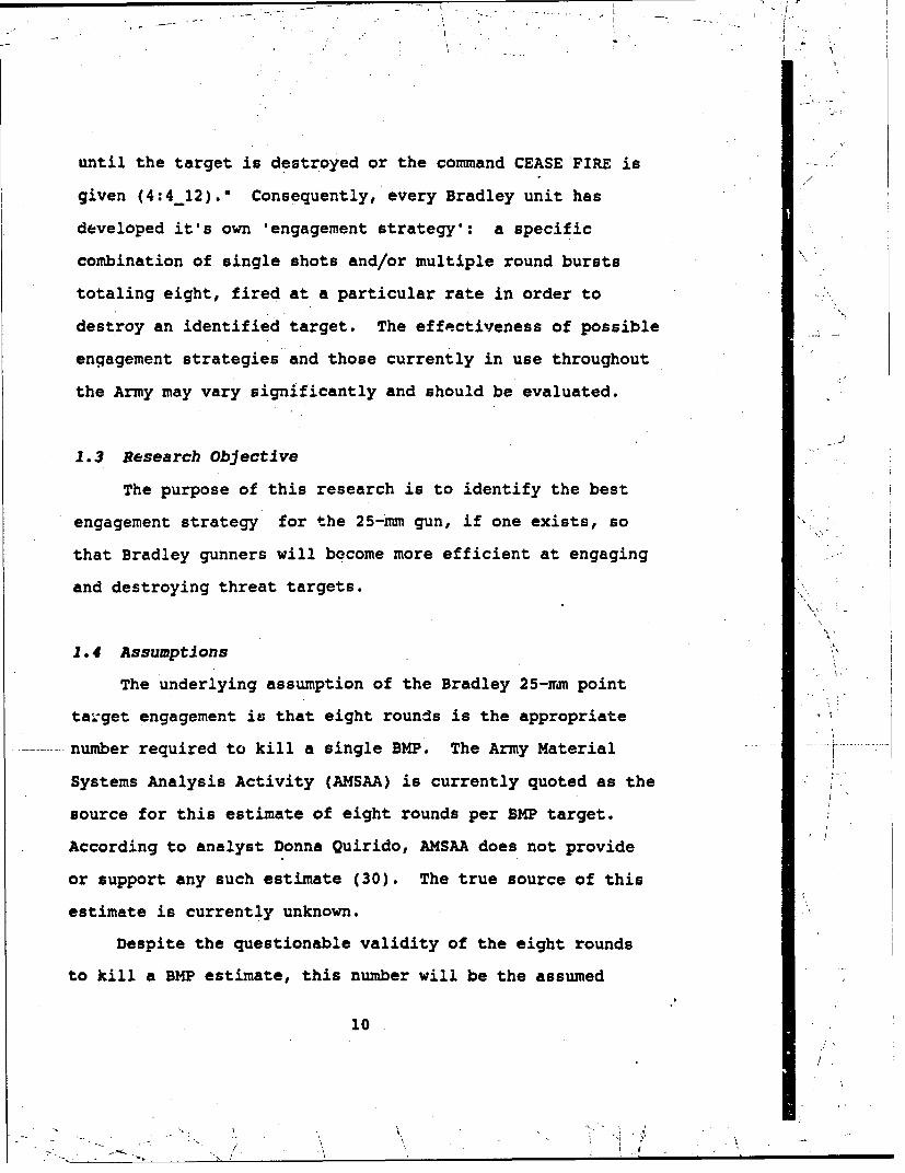
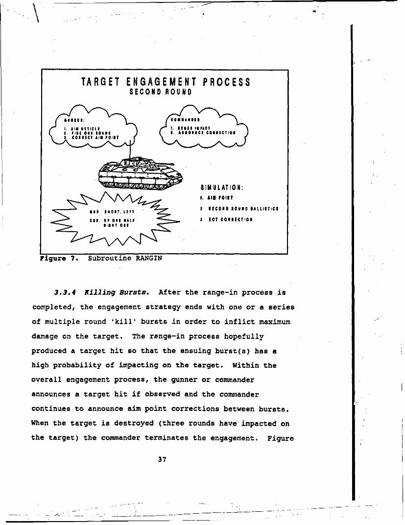
3.3.4 Killing Bursts. After the range-in process is

completed, the engagement strategy ends with one or a series

of multiple round 'kill' bursts in order to inflict maximum

damage on the target. The range-in process hopefully

produced a target hit so that the ensuing burst(s) has a

high probability of impacting on the target. Within the

overall engagement process, the gunner or commander

announces a target hit if observed and the commander

continues to announce aim point corrections between bursts.

When the target is destroyed (three rounds have impacted on

the target) the commander terminates the engagement. Figure

37

-.. . . . . . . . .

8 represents this portion of the engagement and details the

aspects captured by the simulation.

TARGET ENGAGEMENT PROCESS /KILL BURSTS

... $1l INFPA OTS1, 01 1C Al P IN isl l~ 114111111111 OI

' •SIM ULATION:

S. ,1. A,, POINT/

1 1 A 1111[ . M ULT IP L E I O U ID IA L L I IT IC I'

Coo: Bill ? all| NA.F . ACT CORSICTI O/

C f 4. TA10ET &ILL ,

Figure 8. Subroutine KILLBURST

3.3.5 "Fire for Effect. Three rounds impacting on an

actual BMP will probably not result in a mobility or /

firepower kill. The actual estimated numbers are

classified. To achieved the desired level of target

destruction, the Bradley crew will continue to fire multiple

round bursts. As roted, it is assumed these bursts will be

equal in length. The EFFECTS subroutine uses the same 4.

processes as KILLBURST to represent this continuation of the

initial eight round engagement strategy. In order to .'-7

produce a common performance measure for the different x/

38

/

burst lengths, the simulation fires 60 rounds using each of

the three, four, or five round burst patterns.

3.4 A Methodology for Estimating Quasi-Combat Dispersionsfor Automatic Weapons.

The tactical error of the M242 25-mm Hughes chain gunmounted in the Bradley Fighting Vehicle System (BFVS) firingthe M791 APDS-T, and M792 HEI-T rounds will be defined byresidual errors. The term residual error used throughout

refers to the standard deviation about the adjustedcenters of impact of many bursts over many replications. Itincludes all sources of error. This residual error includesprimarily the effects of adjustment between bursts as wellas the effects of ranging in.

3.4.1 Development Test (DT) Dispersions. The DTdispersion tests of the 25-mm M242 weapon were conducted atAberdeen Proving Ground (APG) between April 1978 and June1980. Both hard stand testing of the 25-mm weapon andammunition, and entire weapon system testing from the BFVS.were conducted. The hardstand estimates were based on bothmann barrel and weapon firings which were combined after thestatistical analysis indicated no significant differences.The vehicle testing was conducted under both stationary andmoving firer conditions firing against both stationary andmoving (crossing) targets. The weapon station has astabilization system which allows a high degree of accuracywhen firing on the move. The DT dispersion testing for theBFVS Al vehicle was conducted in Oct-Dec 1984 and is theprimary source for 25-mm dispersions.

These highly controlled'tests were fired using expertcivilian gunners from the Combat Systems TestinS Activity(CSTA), formerly known as Material Testing Directorate (MTD)at APG. The weapon was zeroed at 1000 zm'eters before eachfired test condition. Time-to-fire was\not an element ofthe test. The dispersions are representative of weapon-round repeatability performed under ideal test conditions,and are not necessarily a good representation of thedispersions which would be obtained in a combat situation.The DT dispersions are shown in Table 2. The burst firedispersions are defined with the *shotgun" or "2distribution" model which implies that ea h round in a burstis equally likely to hit the target. The within burstdispersions are the standard deviations about thecoordinates of each round within a burst considering azimuth(AZ) and elevation (EL) independently. The burst-to-burstdispersions are the standard deviations about the centers of

39

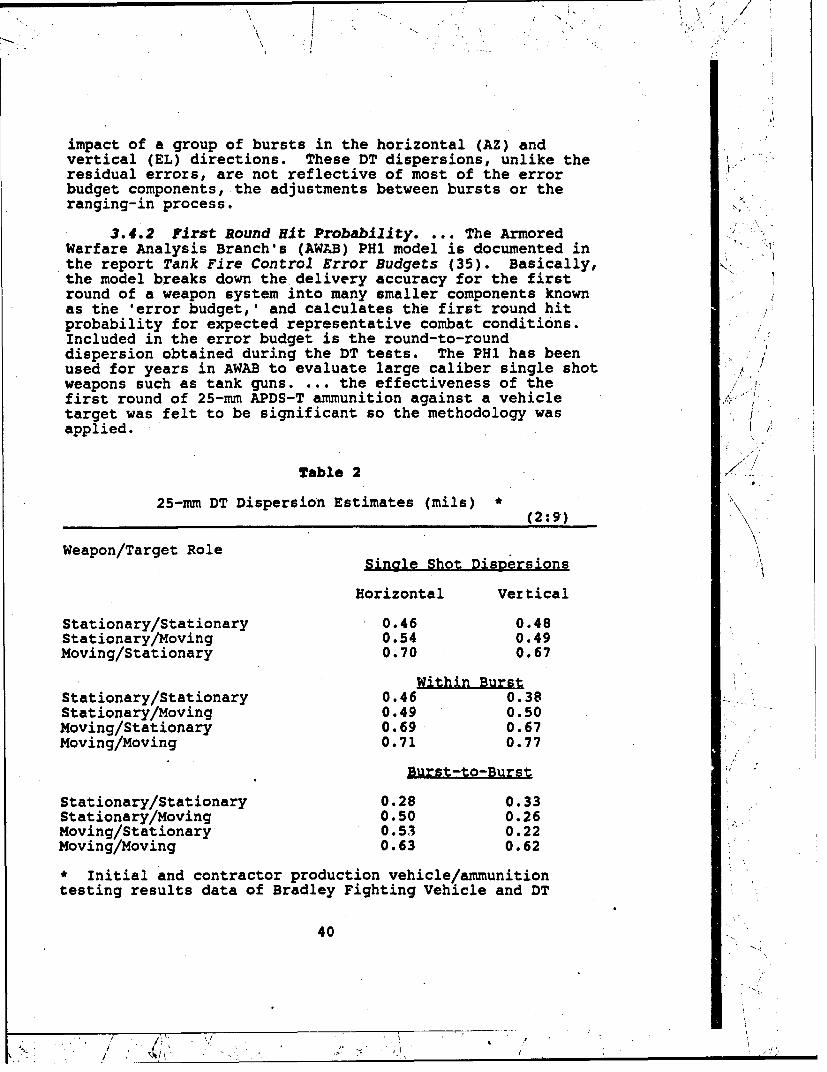
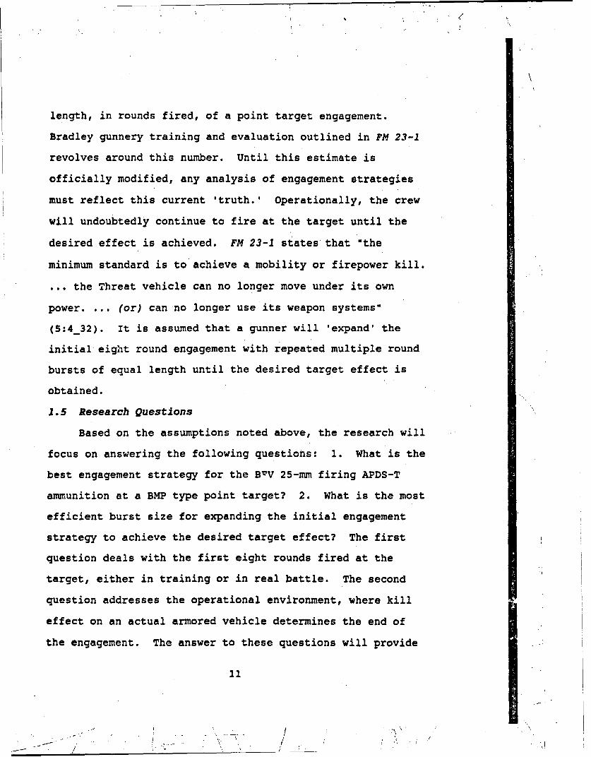
impact of a group of bursts in the horizontal (AZ) andvertical (EL) directions. These DT dispersions, unlike theresidual errors, are not reflective of most of the errorbudget components, the adjustments between bursts or theranging-in process.

3.4.2 First Round Hit Probability. ... The ArmoredWarfare Analysis Branch's (AWAB) PHI model is documented inthe report Tank Fire Control Error Budgets (35). Basically, Kthe model breaks down the delivery accuracy for the first ¶

round of a weapon system into many smaller components knownas the 'error budget,' and calculates the first round hitprobability for expected representative combat conditions.Included in the error budget is the round-to-rounddispersion obtained during the DT tests. The PHI has beenused for years in AWAB to evaluate large caliber single shotweapons such as tank guns. ... the effectiveness of thefirst round of 25-mm APDS-T ammunition against a vehicletarget was felt to be significant so the methodology wasapplied.

Table 2 7

25-mm DT Dispersion Estimates (mils) '(2:9)

Weapon/Target RoleSingle Shot Dispersions

Horizontal Vertical

Stationary/Stationary 0.46 0.48Stationary/Moving 0.54 0.49Moving/Stationary 0.70 0.67

Within BurstStationary/Stationary 0.46 0.38Stationary/Moving 0.49 0.50Moving/Stationary 0.69 0.67Moving/Moving 0.71 0.77

Burst-to-Burst

Stationary/Stationary 0.28 0.33Stationary/Moving 0.50 0.26Moving/Stationary 0.53 0.22Moving/Moving 0.63 0.62

* Initial and contractor production vehicle/ammunitiontesting results data of Bradley Fighting Vehicle and DT

40

/ 4 -.

" / ' ' ~ f...

testing of BFVS Al. AP ammo fired at 100 rds/min in fiveround bursts ...

The PH1 combines the fixed horizontal and verticalbiases of the weapon system with the total dispersions toproduce a first round hit probability. The fixed biases arethe surar.ation of the effects due to parallax (the horizotl.tiland vertical distances from the gunner's sight to the gunbarrel), and horizontal drift of the round caused by spin ofthe projectile. For the APDS-T round, values for parallaxand drift are 0 at (1200) meters since the gunner zeroes theweapon at that range.

The total horizontal (I1) and vertical (V) dispersionsare the root sum squared combinations of the random errors(H+V) and variable biases (H+V). The random errors are theroot sum squared combinations of round-to-round dispersions(H+V) and quasi-combat lay errors (H+V). The round-to-rounddispersions were taken from the stationary BFVS versusstationary target portion of the DT tests (Table 2). Thequasi-combat lay error is attributed to the gunner'sinability to lay the crosshair of a telescopic sight on thedesired aimpoint in a stressed situation. The gunner givesup some precision for a savings in time-to-fire the firstround. This error, which is based on a US time stress testand accepted by a NAIO committee, has been used for manyyears and is valid for any weapon system using a similartelescopic sight.

There are many components which are root sum squaredtogether to produce the variable biases (H+V). Thesecomponents and the values used for the current BFVS firecontrol system are listed in Table 3. Descriptions of thesecomponents can be found in Shiflett's report (35). Thelargest sources of error are range estimation error, cant,and jump. The range estimation error is 17 percent of range

-- for the BFVS fire control with its crude stadia rangefinder. This number is based on test data from similar tankstudies. ... The 17 percent range estimation error is by farthe largest source of error within the total error budgetfor ranges greater than 1000 meters. Cant error is theerror in placing a weapon so that its elevation trunions arelevel resulting in and incorrect aim. The nominal value offive degrees is the largest source of error for thehorizontal variable bias, especially at longer ranges.The occasion-to-occasion jump variable bias is caused bysuch things as tube vibration or angular rotation duringprojectile travel, projectile dynamic and aerodynamicunbalance, and tube bend from uneven heating of the barrel.Additional contributors to jump peculiar to the BFVS may bebacklash, synchronization, removal and replacement of thewiapons from the turret causing loss of boresight, and

41

Integrated Sight Unit (ISU) problems. This occasion-to-occasion jump may vary from occur in both horizontal andvertical directions. ... (2:7-13)

The results from PHI provide the fixed horizontal/vertical

biases and total horizontal/vertical dispersions of the 25-

mm weapons system according to range and will be used in the

simulation model to determine where the first round hits on

the target plane.

/

Table 3

Input Values to PHI for 25-mm APDS-T M791 Round Fired FromM242 Gun Mounted on BFVS .

Zeroed a. 1200 meters(2:11)

H = Horizontal

V = Vertical

Fixed Biases (Meters)/Range (m) Q

Parallax H - -0.6472 0V = -0.4399 0

Drift H = 0.0000 0.18

Random Errors

Round-to-Round Dispersion (H/V) = 0.46/0.48 mils(Stationary/Stationary)Quasi-Combat Lay Error (H+V) = 0.3 meters + 0.05 mils

Variable Biases

Cant (H+V) = 5.0 DegreesRange Estimation Error (V) - 17.0 PercentJump (H) - 0.62 Mils

(V) = 0.33 MilsCrosswind (H) = 11.0 Feet/

Second

Fire Control (H) - 0.11(V) - 0.2 Mils

42

'"/

.\ .• , ->.. , , • ~ ~~~... ;\• -- \",J

• " . ...

Muzzle Velocity Variation (V) = 23.4 Feet/Second

Range Wind (V) = 11.0 Feet/Second

Air Temperature (V) = 8.0 Deg FAir Density (V) = 1.5 PercentOptical Path Bending (V) = 0.03 MilsZeroing (Includes all below) (H+V

Cant (H+V) - 5.0 DegreesRange Estimation Error (V) - 17.0 PercentJump (H) = 0.62 Mils

(V) - 0.3 MilsCrosswind (H) = 11.0 Feet/

SecondFire Control (H) - 0.11 Milseo

(V) - 0.2 MilsMuzzle Velocity Variation (V) = 23.4 Feet/

SecondRange Wind (V) = 11.0 Feet/

SecondAir Temperature (V) = 8.0 Deg FAir Density (V) = 1.5 PercentOptical Path Bending (V) = 0.03 MilsGroup Center of Impact (GCI)(H+V)= 0.21 Mils I'

Observation of GCI (H+V) - 0.05 Mils

3.5 Point Target Engagement Simulation Model Documentation.

As previously defined, an engagement is a combination

of single shots and/or multiple round bursts totaling eight,

fired at a particular rate in order to destroy an identified

target. The engagement strategy further distinguishes a

specific pattern for these eight zounds. Point Target

Engagement models this process. The simulation is

structured to represent the various forms an engagement

strategy might take. It is assumed, based on the ten second

time standard established in FM 23-1 for a single target

engagement, that the shoot-look-shoot nature of Bradley

43

I II

' - I : -"". "" --

gunnery requires an engagement to be limited to four

combinations of single and multiple round bursts. The SLAM

based network provides the basic structure of the simulated

engagement. Ar entity within the simulation represents a

target. Each target is assigned an engagement strategy,

range and width characteristics, and a set of statistical

counters in the form of attributes. See Table 4. The

target processes through four EVENT nodes which represent

the specified combination of single and multiple round

bursts fired and the accompanying adjustment of the reticle

aim point based on BOT between bursts. After each burst is

fired, the target is evaluated to determine if it has been

killed. When the target has been completely engaged with

eight rounds it continues to the COLCT nodes which count the

number of target hits, misses, and kills. The simulation

conducts 100 point target engagements. A flowchart of POINT

TARGET ENGAGEMENT is shown in Figures Al and A2, Appendix A.

44

Table 4

Target Attributes

ATRIB(1) = Number of rounds in first burst

ATRIB(2) = Number of rounds in second burst

ATRIB(3) = Number of rounds in third burst

ATRIB(4) = Number of rounds in fourth burst

ATRIB(5) = Mode: Battlesight of Precision

ATRIB(6) = Range to target

ATRIB(7) = Target aspect (width)

ATRIB(8) = Location of round/burst on horizontal axis

ATRIB(9) = Location of round/burst on vertical axis

ATRIB(10) = Number of target hits

ATRIB(11) = Number of target misses

ATRIB(12) = Target Kill ( > 3 target hits )

3.5.1 Engagement Strategy. Five attributes

distinguish an engagement strategy; attributes one through

four specify the number of rounds the gun will fire in each

of the four possible bursts and attribute five designates

whether the target is engaged in precision or battlesight

mode.

3.5.2 Target Characteristics. Attribute six assigns

the target a range from a uniform distribution between 800

and 1800 meters using SLAM's internal random number

generating capability. It is assumed that the majority of

45

* ----

.-'- , A

engageable targets would present themselves uniformly

between these two ranges without regard to the doctrinal

planning factors of mission, enemy, troops, terrain, and

time (METT-T) which would normally be expected to refine the

range possibilities. Attribute seven assigns the target a

width from a uniform distribution between 2.94 meters (full

frontal) and 6.74 meters (full flank).ý This is a

conservative representation of the full range of possible

target aspects which will be used in an attempt to capture

the non-rectangular nature of the BMP as a target,

especially the area created by the 57 degree frontal slope.

BMP-Type TargetS/ .................... ...... / i............... ................................

29 T 1o• ,, , ,6, / 76.74m -

Figure 9. Target Representation of BMP

According to research conducted by Mike S. Perkins, of

Litton Systems, Inc., "the visible total width of a BMP is

larger between 45 and 90 degrees than it is at 90 degrees

(24:4)." Table 5 lists the complete range of BMP total

visible width as it corresponds to angular orientation to Z'

46

the observer. Note that at 65 degrees the width of the BMP

is actually 7.35 meters,, however, the area near the frontal

slope should not be considered as true target area. While

not geometrically precise, the chosen representation limits

the inflated hit probabilities which would result if the

full range of target aspects were used.

Table 5

Visible Width (mn) of a BMP Oriented at Varied Angles

(24:5)

Target angle Visible front Visible side Visible total-(degrees) width (mn) width (mn) width (mn)

0 2.40.00 2.94

5 2.9.3 0.59 3.52

10 2.90 1.17 4.07

15 2.84 1.74 4.58

20 2.76 2.31 5.07

25 2.66 2.85 5.51

30 2.55 3.37 5.92

35 2.41 3.87 6.27

40 2.25 4.33 6.58

45 2.08 4.77 6.84

50 1.89 5.16 7.05

55 1.69 5.52 7.21

60 1.47 5.84 7.31

65 1.24 6.11 7.35

47

70 1.01 6.33 7.34

75 0.76 6.51 7.27

80 0.51 6.64 ý7.15

85 0.26 6.71 6.97.

90 0.00 6.74 6.74

3.5.3 Statistical Counters.' The simulation tracks the

impact of each round or the center of each multiple round

burst fired at the target using attributes eight and nine to

represent the impact location on the horizontal and vertical-

axis respectively. Conditional ACTIVITIES following each

return from subroutine EVENT records which burst fired

actually killed the target. The number of target hits are

collected from attribute ten, target misses from attribute

eleven, and target kills from attribute twelve.

3.6 Subroutine Event

Subroutine Event controls the seven possible burst

patterns that make up an engagement strategy:

1. No rounds are fired.

2. Single first round burst is fired.

3. Single second round burst is fired.

4. Multiple first round burst is fired. ~

5. Multiple second round burst is fired.

6. Multiple third round burst is fired.

7. Multiple fourth round burst is fired.

48

These seven patterns can be combined to capture all of the

proposed engagement strategies. Based on the designated

engagement strategy, Subroutine Event calls the appropriate

FORTRAN subroutine to represent the type of burst fired and

returns the results of that burst back to the main program.

A flowchart of E¶TENT is shown in. Figures A3 -A5.

3. 7 Subroutine Sense

Subroutine SENSE, Figures A6 -A7, represents a first

single sensing round fired at the target. The aimpoint is

the center of the visible target defined by the standard BMP

target height of 2.2 meters and the variable target width

generated by the main program, Point Target Engagement. The

muzzle of the gun is assumed to be at the same height as the

center of the target. According to Herrmann, in Exterior

Ballistics 1935, "in any practical case the angle of

position is so small that no distinction need be made*

between a gun located above/below the target center and one

which is at the same height. (17:17) The subroutine is

divided into five distinct steps:

1. Computation of First Round Fixed Biases and TotalDispersions.

2. Range Estimation and ISU Index Procedure.3. Calculation of Vertical Miss Distance (VMD).4. Calculation of the Impact Point of the Round.5. Calculation of Aim Point Correction.

on completion of these steps, SENSE determines the number of

target hits, target misses, and the new target aim point and

returns this information to the main program.

49

3.7.1 Computation of Fixed Biases and Total

Dispersions at Target Range. First round fixed biases (FBH,

FBV) and total dispersions (DISPH, DISPV) from PH1 are used

to determine where the first round impacts on the target

plane. The results from PH1 for 100 meter increments

between ranges of 200 and 2000 meters are found in Table 6,

Table 6

RESULTS FROM PH1Fixed Biases and Total.Dispersions (mils)

(31:1-2)

RANGE (M) DISPH DISPV FBH FBV

400 1.2121 1.1081 -1.6926 -1.1202500 1.1190 1.0137 -0.8045 -0.5228600 1.0670 0.9673 -0.5800 -0.3734700 1.0369 0.9485 -0.4182 -0.2667800 1.0198 0.9477 -0.2955 -0.1867900 1.0112 0.9596 -0.1989 -0.1245

1000 1.0084 0.9815 -0.1205 -0.07471100 1.0100 1.0113 -0.0553 -0.03391200 1.0150 1.0479 0.0000 0.00001300 1.0229 1.0906 0.0477 0.02871400 1.0332 1o1389 0.0895 0.05331500 1.0456 1.1922 0.1266 0.07471600 1.0601 1.2505 0.1599 0.09331700 1.0764 1.3135 0.1901 0.10981800 1.0945 1.3810 0.2178 0.12451900 1.1142 1.4531 0.2433 0.13762000 1.1356 1.5297 0.2670 0.1494

Within the subroutine, a linear regression model for each of

these dependent error variables is used to estimate the

biases and dispersions at the appropriate target range.

Computation of the regression models are covered in Appendix

50

C, however, their R-squared values are .9738, .9703, .8715,

and .9880 respectively.

FBH - -1.7834 + .00227RG - 6.453E-07RG2 (21)

FBV- -1. 17336 + .00152RG- 4.424E-07RG2 (22)

DISPR- 1.31464 - 4.955E-O4RG + 2.033E-07RG2 (23)

DISPV- 1.20873 - 5.813E-04 + 3.712E-07RG2 (24)

3.7.2 Range Estimation and ISU Range Index. The

engagement can be fired in either the precision or

battlesight mode. Range estimation is inherent to both of

these firing modes. As previously noted, FM 2L-1 identifies

two battlesight indexes; 1200 for targets within 1400 meters

and 1600 for targets exceeding 1400 meters. It further

recommends a quick range estimation procedure using the

horizontal lead lines to determine when the target lies

within or outside the critical 1400 meter range. (5:3_19-

3_20, 3_28-3_29) It is assumed that the average gunner can

adequately use this method to determine the correct

battlesight range index. The AMSAA standard 17% range

estimation error will therefore be applied to precision and

battlesight engagements since the stadia sight is used in

both methods for range estimation (2:6,10; 18). Given RN3

is a normally distributed random number and the Percent

51

., \ \

/

Range Error (PRE) equals 17 percent, the estimated range is

defined as:

RGEST - RANGE'PRE'RN3 + RANGE (25)

The ISU index range in the precision mode is the

closest 200 meter increment to the estimated range. Based

on conversations with Master Gunners from the Bradley

Gunnery offices at both Fort Benning and Fort Knox, as well

as the authors personal experience, it is assumed that most

gunners would rather index low so their first round, if it

misses, will impact in the dirt. This creates a more

definite signature on which to base their BOT correction

(13). Precision mode index range (INDEX) is defined as:

INDEX - 2 (AINT(RGEST/200)) (26)

The FORTRAN intrinsic function AINT(al) is used to represent

the assumption that the gunner would index the next lowest

range from his estimate.

3.7.3 Calculation of Vertical Hiss Distance on the

Target Plane. Targets will very rarely present themselves

at ranges which correspond exactly to the index settings

available to the ISU. Therefore, even if the effects of

fixed biases and variable dispersions were ignored, most

first rounds would fail to hit the gunner's aim point. To

evaluate whether a particular round impacted on the visible

target plane, the vertical miss distance from the target

52

' "." [ ... ... . •... . • 7 ... . •I-•

center must be estimated. in his book, Exterior Ballistics

1935, Herrmann presents a method for determining this

distance for short ranges using a projectile's angle of

fall. "The angle of fall is the angle between the

horizontal plane (horizontal line from the gun to the point

of aim) and the tangent to the trajectory at the point of

fall" (17:6-7). See Figure 10.

T

/ /0 X H S,

Figure 10. Vertical Miss Distance 4

In Figure 10 the 25-mm gun is located at 0 and a BMP

type target is located at range OH = X. The aim point is

assumed to be at H; the center of target visible mass. The

trajectory OH, representing the gun shooting at a target at

the exact index range, has a point of fall at H and angle of

fall w. The trajectory OH', represents the gun shooting

with an index range greater than the true range to the

target. The point of fall for this trajectory is HO and the

angle of fall is w'. 2' represents the point where the round

crosses the vertical plane of the target. The value of h is

given exactly by the relation h = SO tan z, in which z is

the angle THOH. This angle is unknown, but it appears that

53

v is approximately equal to z, and that h can be defined by

'the relation:

h - S' tan(w (27)W

in which w is the angle of fall corresponding to the true

.target range. Herrmann states: "Although no rigorous proof

of equality between the angles w and z is available, it has

been established by exhaustive comparative solutions that

these angles are indeed very nearly equal in any practical

situation." (17:270) Equation (27) will be used within the

simulation to determine vertical miss distance VMD (18;

17:268-270). Angle of fall values for 25-mm APDS-T

ammuni.tion comes from Ballistics ResearchLaboratory data

dated November 1983 (1:1-2).

3.7.4 Computation of Impact Point. ISENSE now

determines where the round hits on the tarzget plane. The

aim point (XAIM,YAIM) is the center of the predefined

rectangular target. For the first round only the first

round fixed biases and total dispersions derived from PHi

along with the vertical miss distance are used to determine

the impact point. Letting RMI and RN2 be normally

distributed random numbers (N(O,1)), the equations used to

determine the impact coordinates (XA,YA) for the first round

are:

XA - XAIM+ FBHOR + RNI'DH (28)

54

; ... . ' I

, ' "- .. . I

YA- YAIM + VAM + FBVEP + RN2"IV (29)

whereVMD = Vertical Miss Distance

FBHOR = Fixed Biases HorizontalFBVER = Fixed Biases Vertical

DH = Total Dispersions HorizontalDV = Total Dispersions Vertical

The X and Y miss distances become:

XMISSD - XA - XAIM (30)

YMISSD - YA - YAIM (31)

The subroutine evaluates these miss distances against the

target critical area to determine if a hit has occurred.

The target critical area (XLIM,YLIN)is defined by the

relations:

XLIM - TGTW/2 (32)

YLIM - TGTH/2 (33)

where

TGTW = Target width

TGTH = Target height

The number of hits (NHITS) and misses (NMISS) are recorded.

3.7.5 Burst on Target (BOT) AdjLstment Process. As

previously defined BOT is a direct fire adjustment technique

in which the gunner and vehicle commander observe where the

round strikes in relation to the target and convert the

relationship into an executable correction for the original

55

- 1• .. I-• " - \

point of aim. The currently accepted method for modeling

this process is based on data obtained from the YAKIMA

firing test conducted in support of the Infantry Warfare

Analysis Branch's (IWAB) BUSHMASTER study. However,

only the 20mm M139 gun mounted on an XM701 having GE(Weapons Contractor: General Electric) stabilizationwas fired at YAKIMA. The data provided is consideredto be 'ball park' for the 20-30mm MICV (MechanizedInfantry Combat Vehicle) systems, but obviously cannotbe guaranteed to be applicable to the current BFVS.The maximum range utilized in the test was 1800 meters.Extrapolation beyond 2000 meters may be risky. (2:18)

While further analysis is warranted to verify its

representation of the actual BOT correction distribution,

the YAKIMA method will be used throughout this simulation

model. The YAKIMA data quantifies the correction of miss

distances in terms of mean percent correction and standard

deviation. The final mean correction was 0.4 of the miss

distance with a standard deviation of 0.7. The correction

algorithm is defined as:

XA - (0.4 + 0.7RN1)XMISSD + XATM (34)

/YA - (0.4 + 0.7RtN2) YMISSD + YAIM (35)

where XA and YA represent the coordinates of the next round

impact point. A flowchart of SENSE is shown in Figures A6 -

A7.

A

3.8 Subroutine RANGEIN

Subroutine RANGEIN represents the firing of a second

single sensing round at the target. It uses the new impact

56

1k

/''\

SY p -" " - . -"

point generated by subroutine SENSE and incorporates the

weapon system's round-to-round dispersion factors to compute

the second round impact point. RANGEIN uses the DT test

round-to-round dispersions to determine the weapon system

delivery error for the second round. Using random numbers

RNI and RN2, the round-to-round delivery errors are defined

by the equations:

SDXERR - RNI • SDXZZ (36)

SDYERR - RN2 * SDYZZ (37)

The delivery errors are used to compute the impact

coordinates of the round based on the aim point (XA,YA) from

SENSE:

XA - XA + SDXERR (38)

YA - YA + SD YERR (39)

The subroutine determines whether the round hit or misses

the target and applies the YAKIMA adjustment method using

the previously defined algorithms; Equations (34) and (35).

The number of target hits, target misses and new target

impact point are returned to the main program. A flowchart

of RANGEIN is shown in Figure A9.

3.9 Subroutine FRSTBURST

Subroutine FRSTBURST represents the firing of a

multiple round burst without a prior sensing round. It uses

57

- .\

the same procedural steps as subroutine SENSE, but

incorporates the burst-to-burst and within-burst dispersions

of the weapon system into the calculation of the individual

round impact points. The DT test values for these "\

dispersions are used. As noted in the description of the DT

test, the within-burst dispersions are defined by the

'shotgun' model which implies that each round within the

burst has an equal probability of hitting the target. An

analysis of individual round impact data obtained during

live-fire testing conducted by Ground Warfare Division,

AMSAA confirmed that there is no significant auto-

correlation or systematic dependence between :-ounds. (13)

The results of this analysis are included in Appendix D.

Modeling a multiple round burst requires that two of

the processes defined in SENSE be modified: computation of

impact points and aim point adjustment.

3.9.1 Computation of Multiple Round Impact Points.

Subroutine FRSTBURST must compute and evaluate the impact

point of each round fired in the burst to determine if it

hit the target. Since these are the first rounds fired at

the target, the first round fixed biases and total

dispersions derived from PH1 along with the vertical miss

distance are used to determine the impact points using the

same equations (28) and (29) defined in SENSE . FRSTBURST

uses the DT test round-to-round and the within-burst

dispersions to determine the weapon system delivery errors

58

/ A

for each round. Using random numbers .I and RN2, the

round-to-round and within-burst de livery errors are defined

as:

SDXERR - RN1 SDXZZ (40)

SDYERR - RN2 SDXZZ (41)

//SCXERR - RN1 SCXSS (42)

/

SCYEER - RN2 SCYSS (43)

The delivery errors are used to compute the impact

coordinates of the individual rounds by adding them to the

impact points XA and YA determined with equations (28) and

(29):

XAFER - XA + SDXERR + SCXERR (44)

YAFER - YA + SDYERR + SCYERR (45)

The subroutine determines whether each round hit or misses

the target and accumulates the totals to return to the main

program.

3.9.2 Burst on Target (BOT) Adjustment Process.

FRSTBURST uses the YAKIMA adjustment algorithm, however, the

adjustment is applied to the burst center of impact. It is

assumed that gunners and Bradley commanders would evaluate

the location of the combined burst impacts as opposed to

identifying a single round, first or last round perhaps, on

which to base their BOT correction. The burst center of

59

impact is defined as the mean impact coordinates for the

number of rounds in the burst:

XA = SMXIXN/RS (46)

YA . SmI NRES (47)/

whereNRBS = Number of rounds in the burst

SMX = Sum of horizontal axis impact coordinatesSMY = Sum of vertical axis impact coordinates

The YAKIMA adjustment algorithm is applied the center of

impact using equations (34) and (35) defined above. A

flowchart of FRSTBURST is shown in Figures A10 - A12.

3.10 Subroutine KILLBURST

Subroutine KILLBURST represents the multiple round

burst(s) a gunner uses to kill the target. The range in

process has technically ended, although it is assumed that

the gunner and Bradley commander will continue to use BOT to

fine tune the-round impacts on the target. KILLBURST uses

the same methodology as subroutine SENSE, but incorporates

the burst-to-burst and within-burst dispersions of the

weapon system into the calculation of the individual round

impact points. The DT test values for these dispersions are

used and applied in the same manner as in subroutine

FRSTBURST. The BOT adjustment process is modeled using the

YAKIMA algorithm as defined by equations (46), (47), (34)

and (35) in FRSTBURST. The resulting accumulated target

60

hits, target misses and adjusted aim point coordinates are

then returned to the main program. A flowchart of KILLBURST

is shown in Figures A13 - A14.

3.11 Subroutine EFFECTS

Subroutine EFFECTS uses the same procedures as

KILLBURST. A DO-loop is added to allow the firing of a

designated number of multiple round bursts.

3.12 Validation and Verification

As noted earlier, POINT TARGET ENGAGEMENT uses

virtually the same structure and algorithms as AMSAA's

HITPROB2 model to represent the Bradley 25-mm gun systent.

Whereas HITPROB2 is a replications model, the simulation in

this research is designed to model single discrete

engagements. Delivery error parameters within the

simulation are based on accredited AMSAA data from their PHl

model. The vertical miss distance algorithm was modified

slightly because the AMSAA version could not be documented.

The resulting calculations, documented from Herrmann (17),

will probably provide a more conservative estimate.

The SLAM based shell of the model allowed for a logical

and systematic verification process. Using a single target

replication, several engagements were created round by round

to test the shoot-look-adjust-shoot representation of the

61

gunnery process. This iterative approach confirmed the

following:

a. Target range and aspect changed with each new

engagement.

b. Firing mode selection occurred and resulted in

different first round impact points.

c. Single and multiple round burst locations were

recorded.

d. The aim point correction process resulted in

improved impact points for subsequent rounds.

e. The statistical counters functioned properly.

Complete validation of the simulation is impossible,

however, the outputs appear to be credible and consistent

with AMSAA's results in other but related Bradley studies

(2:16,36; 18; 29).

62

ZV. Nethodology

4.1 Introduction

This chapter discusses the methodology that will be

used to answer the research questions: 1. What is the best

engagement strategy for the BFV 25-mm firing APDS-T

ammunition at a BMP type point target? 2. What is the most

efficient burst size for expanding the initial engagement

strategy to achieve the desired target effect? An outline

of the proposed research process is presented followed by a

description of the experimental design used to analyze the

model outputs. The selected measures of effectiveness (MOE)

will be discussed along with a theoretical description of

the output analysis techniques to be used in determining

relative performance.

4.2 Research Procedure

The research effort began with a literature review of

weapon system modeling, summarized in Chapter 2, to identify

techniques appropriate for representing the Bradley's 25-mm

gun. The AMSAA model HITPROB2 provided the basic structure

for a simulation designed to answer the specific research

questions. AMSAA was reviewing two aspects of this model,

the Aim and Aimpoint Adjustment (AAA) algorithm and

ballistic dispersion parameters, which would impact similar

portions of the research specific simulation.

63

/.\

They conducted live-fire testing using M791 ammunition

during the period 12-16 September 1992, the results of which

were included as appropriate (12:1,6; 13).

Since there are numerous engagement strategies possible

and known to be in use throughout the Army, a letter

requesting input from the Bradley community was submitted to

the January-February 1993 issue of INFANTRY magazine. The

responses from this inquiry will be added to the strategies

known from the author's personal experience and evaluated

using the simulation model.

The results were evaluated using the statistical

procedures outlined below.

4.3 Experimental Design

The model, POINT TARGET ENGAGEMENT, simulates the

Bradley gunnery process. It provides output data, which

represents quantitative measures of 25-nun gunnery

performance, in the form of a probability distribution of

accumulated target hits or alternatively total targets

killed. The random variation inherent in Bradley gunnery

performance is influenced by a number of factors, some whic h

can be controlled and some that cannot. See Figure 11.

64

Controllable Factors:- Engagement Strategy- Firing Mode

Dependent Response:-Targets Killed

E - Target Hits

Uncontrollable Factors:- Range to the Target- Range Estimation Error- Delivery Errors- YAKIMA Adjustment Algorithm

Figure 11. Bradley Gunnery Process

Each of the input factors influences the performance of

the gunnery process to some degree. Of the controllable

factors depicted, the engagement strategy used during a

single BMP-type target engagemen~t is the focus of the two

research questions. We would li e to determine if the

influence or effect of using a particular engagement

strategy significantly improves gnnery performance or if

some engagement strategies are si ificantly better than

others. Figure 12 shows the type sf relationship we hope to

capture.

65

Engagemient StrategiesA a

Usa U1, d U, U*

Target Kills

Figure 12. Distribution of Target Kills by EngagementStrategy

However, because firing mode, precision/battlesight, is /also a controllable aspect of gunnery, we must also

determine its significance and whether an interactive

relationship exists between engagement strategy and firing

mode. It is assumed that gunnery performance in precision

mode will be better than in battlesight mode. The

additional accuracy in estimating the location of the target

found in precision mode procedures should result in a higher

level of target hits/kills regardless of the engagement

strategy used. However, if an inte.Ljctive relationship

exists between firing mode and engagement strategy, the

anticipated improvement between firing modes would change

depending on the engagement strategy used. Figure 13

graphically shows the two possible situations.

66

//

D CT T

Taretll e g/q ,n

C D

CE

Figure 13 EnagmetStategy -Firing Mode Interaction"

In Figure 13a, there is no interaction present. Target

kills increase uniformly as the firing mode changes from

battlesight to precision mode. In Figure 13b, interaction

* I

is present. Target kills still increase as the firirg mode

changes, but the increases differ according to theengagement strategy used.

The YAKIMA Aim Point Adjustment Algorithm, although

considered as uncontrollable factor in that it models

relative human performance, is also a point of concern for

this research. It has been identified as the weak link in

AMSAA's HITPROB2 model and therefore must be considered a

question mark in the validity of POINT TARGET ENGAGEMENT as

well. (29:3; 2:18) An additional research question istherefore: If the YAKIMA method is wrong, how does a change

to the algorithm influenclhefo interpretation of the model's

results? For the purpose of experimentation, this factor

67

- /" \

• ,,

can be fixed at various levels in order to test the

significance of the YAKIMA algorithm as a contributing

factor and whether it will interact with the engagement

strategy factor as well. A strong interaction would

indicate that our results must be interpreted based on an

assumption that the YAKIMA algorithm is correct. Refer to

Figure 14.

70 S 70 a

A A60 s

0 -- A T0-* IE

C

40- 40-

F~~fr~~g (a) IkQMd

To"g lam Twig lKlNwMAodlhm

70 a 70--T B

AA

a0 so

A E

40- 40-

MV Mode f *f

Figure 14. Interpretation of Engagement Strategy -YAKIMA

Algorithm Interaction

68

Figure 14a shows the potential effect of the YAKIMA

algorithm as a significant factor wihu interaction. The

change to the algorithm produces a uniform improvement for

each of the engagement strategies. The model, under these

conditions, would be considered sensitive to the algorithm

assumption, however, the relative performance of the

engagement strategies would remain consistent for all forms

of the aim point adjustment algorithm. Figure 14b shows how

the presence of a strong interaction between the YAKIMA

algorithm assumption and engagement strategy would

complicate and confuse the analysis. The amount of

improvement depends on both the change in the algorithm and

the particular engagement strategy.

These three factors, engagement strategy, firing mode,

and aim point adjustment algorithm, will be used to quantify

or explain a portion of the total variance within modeled

gunnery performance. The remaining "actors depicted in

Figure 11, range to the targets, range estimation error, and

weapons delivery errors, are assumied to be uncontrollable

and remain sources of unexplained variance in the gunnery

process.

The various statistical tests conducted to answer these

research questions are applications of analysis of variance

methods. Analysis of variance (ANOVA) models are

statistical tools for studying the relation between one or

more independent variables and a dependent response

69

Af

variable. ANOVA methods allow us to characterize the ii-various sources of variance in the Bradley gunnery process

and determine how a single factor or combination of factors

influence relative performance. A multifactor study, in

which the effects of two or more factors are investigated

simultaneously, is used to answer the first research

question and to perform the sensitivity analysis on the

YAKIMA algorithm assumption. The second research question

is addressed using a single factor study. The designs for

these experiments follow. -

4.3.1 Research question #1: What is the best'

engagement strategy for the BFV 25-mm firing APDS-T

ammunition at a BMP-type point target?

As discussed above, in order to answer this question we

must determine if any interactions exist that will

complicate the analysis of how the various engagement

strategies effect performance. For this reason, tests for

two and three factor interactions are conducted first. The

goal is to isolate the engagement strategy factor and

determine whether one particular strategy or a group of

stra egies will maximize the mean number of target kills.

4.3.1.1 The model. Target kills will be the

dependent variable. As defined in FM 23-1, success for a

BMP-t e single target engagement in Bradley gunnery is the

3-round 'kill' (5:11_5). Additional rounds impacting on the

target, while certainly relevant in an actual combat duel

70-I\

- *1* / ;-~K ,/ '

with a BMP, have no real meaning in the training

environment. This aspect of the initial eight-round

engagement strategy will not be evaluated.

The independent variables or factors are engagement

strategy, firing mode, and aim point adjustment algorithm.

The following seven engagement strategies will be evaluated

as levels of the main factor:

A. 1 - 1 - 1 - 5 E. 1 - 2 - 5B. 1 - 2 -4 F. 1- 3 -4C. 1- 1 -3 -3 G. 2- 3 -3D. 1-2-2-3 2

The strategy (1 - 4 - 3) was dropped from the model because

it proved to be statistically equal to (1 - 3 - 4) using . '

target kills as an MOE.

There are 35 possible combinations of eight rounds

under the assumption that no more than four sl~oot-look-

adjust-shoot procedures were feasible within the ten second

time constraint for a single target engagement specified in

FM 23-1 (5:11_29). These seven strategies were selected

from those possible based on the author's gunnery

experiences as the commander of a Bradley equipped infantry

company and conversations with Master Gunners from Fort

Knox, Yentucky and the Bradley Proponency Office at Fort

Benning, Georgia (13). This list may not include every

strategy currently in use throughout the Army, but merely

the most common as they could be determined by the author.

-7

71

S* . . , . . . . _

The second factor, firing mode, will be categorized at

two levels according to either precision (P) or battlesight

(B) engagement procedures. ..

The third independent factor represents the YAKIMA aim

point adjustment algorithm. The factor will be tested at

three levels reflecting the algorithm as it currently

appears in POINT TARGET ENGAGEMENT and the algorithm with a

higher and lower mean correction value. The assumption is

that the YAKIMA algorithm either over- or underestimates the

average Bradley crew's ability to apply BOT adjustment

procedures. The resulting test levels for the algorithm

are:

L XA - (0O. 7 + O. 7 RN1) XMISSD + XAIM%1YA - (0.7 + 0.7RN1) YMISSD + YAIM (.8

M -XA - (0.4 ÷0.7RN1)XMfISSD + XAIM (49)YA - (0.4 +0.7RN1) YMISSD + YA IM

H - XA - (0.2 + 0.7RNI)XMISSD+XAIM (50/YA - (0.2 +0.7RN2) YMISSD+ YArIM

The remaining factors which influence gunnery

performance; range to the target, range estimation error,

and weapon system delivery errors are assumed to be captured

in the error term.

The linear statistical model is therefore:

* ~+ z i + j +yk +( ij +(y) k + y) t+ (ry) jke.,, (5 1)

72

where the factor effects are defined by

-- engagement strategy A ... GS- firing mode P or Byk - algorithm L , M or H

() ij- strategy/mode interaction(T)k •- strategy/algorithm interaction(y)j .- mode/algorithm interaction

(TPY)ijk - strategy/mode/algorithm interaction- random error for all 1 replications

4.3.1.2 The hypotheses tests. Seven tests are

possible using the three-factor model, however, only six are

of particular interest.

1. Do engagement strategy and algorithm interact?

H0 : (-rY)I" - 0 for all i,k (52)He: at least one (y)ik * 0 .

2. Do firing mode and algorithm interact?

Ho: I 3y)jk - 0 for all j,k (53)Ha: at least one (Py)jk * 0

3. Do engagement strategy and firing mode interact?

Ho: (T) " 0 for all i,j (54)Ha: at least one (P) Ij o 0

4. Are the effects of the algorithms significant?

Ha: at least one yk7 0 (55)

5. Is there a difference between firing in precision and

battlesight mode?

H: at least one P.* 0

73

6. Are the engagement strategies different?

Ho: '& - A T • g- 0 (57)Ha: at least one T., 0

4.3.1.3 Level of significance and sample size.

Sample size for the experiment was determined using the

power approach as outlined by Neter, Wasserman, and Kutner

in Applied Linear Statistical Models (21:846). A single

simulation run results in the number of tazgets killed out

of 100 possible. There are 42 treatment combinations based

on seven engagement strategies, two firing modes, and 3

levels of the algorithm factor. In order to detect a one

standard deviation difference in. the main effects, while

limiting the risk of making a TYPE I error to .05 and a TYPE

II error to .30, 144 replications for each of these

treatment combinations are appropriate.

4.3.1.4 The test statistics. The total sums of

squares for this model can be decomposed into the sums of

squares for each factor, two-way interaction, three way

interaction and the sum of squares due to error.

SST - SSatzategy + SSode + SS 1goithm + SSratey/md."+ SS&CeaCgy/a'gorfthm + SSd,/g,.th (58)"+ SSaezategy/ode/algor1thm + SSEr

The associated degrees of freedom are:

strategy: (7-1) -6mode: (2-1) -1

algorithm: (3-1)-2strategy/mode: (7-1) (2-1) -6

strategy/algorithm: (7-1) (3-1) -12mode/algorithm: (2-1) (3-1) -2

strategy/mode/algorithm: (7-1) (2-1) (3-1) -12Error: (7) (2) (2) (72-1) -6006Total: (7) (2) (2) (144)-1-6047

74

Each sum of squares dixided by its respective degrees

of freedom is the mean square. Under the assumption that

the model, equation (51), is adequate and that the error

terms are normally and inJependently distributed with

constant variance, the following ratios of mean squares form

the appropriate test statistics:

1. Do engagement strategy and algorithm interact?

FO - NS~trate/alfrit (59)MSH

2. Do firing mode and algorithm interact?

F - MSE•e/algoritth (60)MSW

3. Do engagement strategy and firing mode interact?

F, - Msatzaegy/mo (61)MSE

4. Are the effects of the algorithms significant?

MS1g'chFO- Malgzih %62)MSE

5. Is there a difference between firing in precision and

battlesight mode?

F, - MSm.. (63)MSE

6. Are the engagement strategies different?

FO - Mt.ragy (64)

4.3.1.5 Multiple Comparisons. Should the tests

above indicate the engagement strategies are not the same,

multiple pairwise comparison tests of the factor mean

75

S.>

responses, or if interactions exist the treatment level

means, will indicate their specific differences. Neter,

Wasserman, and Kutner point out the following limitations of

simple comparison of means testing.

1. The confidence coefficient 1 - a applies only to a

particular estimate, not to a series of estimates.

2. The confidence coefficient 1 - a is appropriateonly if the estimate was not suggested by the data.(21:579)

The Tukey HSD procedure will be used for these tests in

order to hold the family confidence coefficient constant at

.95 (21:580-583, 837).

4.3.2 Research Question 12. What is the most

efficient burst size for expanding the initial engagement

strategy to achieve the desire target effect?

A fire for effect phase to an engagement assumes that

the initial eight rounds resulted in at least one target

hit. Based on that assumption, the only controllable factor

which might influence the Bradley gunnery process is the

length of the killing burst. A single factor ANOVA

experiment provides the means to compare the three burst

,lengths and determine if a 'best' kill burst exists within

the limitations of this research.

4.3.2.1. The model. The second research question

will be analyzed using the accumulated target hits out of 60

total rounds as the dependent variable. without addressing

the classified estimates of how many APDS-T rounds are

76

required to neutralize the various BMP versions, the

accumulated number of target hits appears to be an adequate

measure of effectiveness.

The single factor is the length of the killing burst in

number of rounds. The three factor levels are: A = 3

round burst; B = 4 round burst; C = 5 round burst.

The linear statistical model is therefore:

Y•j - p. +ejjk (65)

where

Tj - burst length a ... cejj - random error for all j replications

4.3.2.2 The hypotheses test.

Are the effects of the bursts different?

Ho: a " b" •" 0(66)Ha: at least one - 1 #., 0

4.3.2.3 Level of significance and sample size.

Sample size for the experiment was also determined using the

power approach. In order to detect a one standard deviation

difference in the main effects, while limiting the risk of

making a TYPE I error to .05 and a TYPE II error to .10, 27

replications are appropriate for this single factor

experiment.

4.3.2.4 The test statistic. The total sums of

squares for the model can be decomposed into the sum of

77

vc-

squares for the single factor and the sum of squares due to

error.

SST -SSb=,a + SS, (67)

where the associated degrees of freedom are:

burst: (3-1) -2Error: (27-3) -24Total: (27-1) -26

Each sum of squares divided by its respective degrees.

of freedom is the mean square. Under the assumption that

the model, equation (65), is adequate and that the error

terms are normally and independently distributed with

constant variance, the following ratio of mean squares form

the appropriate test statistic:

F,, M~bra~,(68)Fo MS,

4.3.2.5 Multiple Comparisons. Should the test

above indicate the mean number of hits according to burst

length are not the same, the Tukey HSD procedure also will

be used for multiple pairwise comparisons in order to hold

the family confidence coefficient constant at .95 (21:580-

583).

4.3.3 Model Adequacy. The inferences gained from the

ANOVA methods can only be used if the underlying models

prove adequate. The two ANOVA model assumptions will be

checked using residual analysis. A normal probability plot

of residuals will be used to determine if the error terms

78

are normally and independently distributed. The constant

variance assumption will be verified using plots of the

residuals versus the fitted response values and engagement

strategies. (20:210-213; 21:609-611,613-614)

79

LS

V. RESULTS

This chapter summarizes and discusses the results from

the experimental design outlined in Chapter 4. The

discussion is divided into two parts which correspond to

Research Questions 1 and 2. The results are addressed in

relatively generic terms, with only limited explanation as

to how they relate to Bradley gunnery techniques. Specific

conclusions about the practical ¶ignificance of the findings

and their potential impact on gunnery will be discussed in

Chapter 6.

5.1 Research Question 11. What is the best engagement

strategy for the BFV 25-mm firing APDS-T ammunition at a

BMP-type target?

Eight hypothesis tests were purposed in order to answer

this question. The first four determine if any significant

interactions exist; the presence of which would complicate

the analysis. Specifically, the tests determine the \ /

sensitivity of model results to changes in the YAKIMA Aim

Point Adjustment Algorithm. Based on the results of these

tests, the fifth test checks the significance of using the

precision versus battlesight mode of target engagement. The

final test, as well as follow-on multiple comparison tests,

focus on determining if a 'best' engagement strategy exists.

The ANOVA table below summarizes the results.

80

-':i

/ .

//

Analysis of Variance Procedure

Dependent Variable: TARGET KILLS

Sum of Mean FSource DF Squares Square Value Pr >F

Model 41 192133.2 4686.2 215.8 0.0001

STRATEGY 6 89522.6 14920.4 687.2 0.0001ALGORITHM 2 88102.2 44051.1 2028.9 0.0001MODE 1 6812.8 6812.8 313.8 0.0001ALGORITHM*STRATEGY 12 5780.7 481.7 22.2 0.0003ALGORITHM*MODE 2 1700.9 850.5 39.2 0.0001MODE*STRATEGY 6 113.1 18.9 0.9 0.5463ALGOR*MODE*STRATEGY 12 100.8 .4 0.4 0.9687

Error 6006 130399.8 21.7

Total 6047 322533.0

5.1.1 Influence of YAKIMA Aim Point Adjustment

Algorithm. Assumptions concerning the validity of the

Yakima algorithm will significantly influence the

conclusions that may be drawn from this research. Although

the three-way interaction (algorithm/mode/strategy) is not

significant, the ANOVA results show a significant

interaction of the algorithm factor with both firing mode

and engagement strategy. The main factor effect is also

highly significant. As noted in Chapter 4, the presence of

an interaction between the algorithm factor and engagement

strategy means that the model results are not robust to

changes to the aimpoint adjustment algorithm. As a result,

the engagement strategies may only be evaluated within a

specific level of the algorithm factor. Interpretation of

the model's sensitivity to the YAKIMA algorithm assumption

81

S~/

can be enhanced using a graphic representation. See Figure

15.

7I0-- SION BATaLESGT 70

, C I IC,I 'D I 'c .

GsA ' D3 'A/( 65

P BY

C I

55 3 ' 0/5

A ' 0 C'

3'--

ALI A:

I I I

Fgr15. Inepetto ofteYKM supin onoe

I '

Results

The graphs highlight the dramatic and intuitive

influence changes to the algorithm factor levels have on

overall performance regardless of the various engagement

procedures employed. This represents the influence of the

main factor effect. An average aim point correction of 30

percent of target miss distance (L) yields extremely low

results in relation to an average correction of either 60

percent (M) or 80 percent (H).

82

- -

Changes to the algorithm levels have a greater

influence on performance in the battlesight •iode than in

precision mode as evidenced by the steeper slope of the

connecting lines. This result is also intuitive.

Battlesight procedures depend on a relatively conservative

GO/NO GO type of range to target estimation. The resulting

ISU index range of either 1200 or 1600 meters creates an

inherently larger initial aiming error. In contrast, the

additional accuracy in target range estimation using

precision gunnery procedures decreases the initial miss

distance due to aim error. Therefore, the required aim

point adjustments in the battlesight mode will usually be

larger and more significantly affected by the accuracy of

the adjustment procedure. It should be noted, however, that

as the adjustment procedures improve, the difference in

relative performance between firing modes is less

pronounced. The mean target kills over all engagement

strategies for each combination of algorithm and firing mode

are listed below.

Level of Level of MeanALGORITHM MODE TARGET KILLS

H P 62.95

H B 62.02

M P 60.05

M B 58.11

L P 55.00

L B 51.49

83

The algorithm/engagement strategy interaction also

exhibits a reasonable set of trends which the graphs

highlight. As the aim point algorithm improves in accuracy

those engagement strategies which consist of four shoot-

look-adjust-shoot combinations and/or employ more than one

sensing round show a more dramatic improvement in the number

of target kills. The slope of the connecting lines for

these strategies (A, B, C, D) are much steeper. Since the

range-in process is extended in these strategies, the aim

point has been further refined prior tQ firing the first

killing burst; resulting in an improved hit probability for

these subsequent bursts. This result i• consistent with

AMSAA's findings using the HITPROB2 model to determine a

distributioi, for the number of rounds required to range-in

targets at various fixed ranges. Table 17 shows AMSAA

estimates for the probability of range-in based on tA.e

number of sensing rounds fired and the average number of

rounds required to range-in targets at various ranges.

84

TABLE 7

Cumulative Range-in Probabilitiesand

Average Number of Range-in Rounds(18:6-7)

Range Number of Range in Rounds Average I1 2 3 Required

800 0.952 0.979 0.991 1.2

1200 0.813 0.904 0.947 1.8

1600 0.619 0.772 .0.867 2.6

2000 0.444 0.625 0.754 3.5

The results depicted in Figure 15 also lead the

research directly back to the YAKIMA algorithm itself. As

noted in Chapter 3, AMSAA's documentation states that the

YAKIMA method

quantifies the correction of miss distance. Thequantities calculated are the mean percent correctionof the miss distance on the preceding round, and thestandard deviation thereof. ... The final meancorrection was 0.4D with a standard deviation of 0.7Dwhere correction is the adjustment made. (2:18)(emphasis added)

The coded algorithm, however, actually calculates the impact

coordinates for the next round based on a mean correction of

60 percent rather than 40 percent. See Figure 16.

YAW

YAKIA Documsntato

Coaeme Aim Point

YAIMA Codtto

(---Ca)C Ai POW imlUn'. X ).YAM2 Poin fo ahm

ACYWSSD) Yakina Mim Point

A4 mmat AlOSr mi __-XA(1). YA(1)

"+ iT round

AOUSSD)Impact Point

Figure 16. YAKIMA Aim Point Adjustment Algorithm

The author's practical Bradley gunnery experience leads

to the assumption that the coded algorithm is a more

accurate representation of an average Bradley crew's ability

to apply BOT adjustment procedures. The remainder of the

results presented will be based on that assumption. The

obvious discrepancy between the coded algorithm and the

written documentation only serves to place additional

emphasis on understanding the potential influence of the

YAKIMA algorithm proving to be incorrect.

5.1.2 Firing Mode Influences. The ANOVA results

indicate that the difference in performance between

precision and battlesight mode engagements is statistically

significant. As noted above, however, the level of

86

N4 I.

significance is also dependent on the accuracy of the aim

point adjustment algorithn. Further, the results show no

significant interaction between firing mode and engagement

strategy.

5.1.3 Influence of Engagement Strategies. The ANOVA

table shows a significant difference exits between the

various engagement strategies. The nature of these

differences become apparent from the results of multiple

pairwise comparisons using the Tukey Honestly Significant

Difference (HSD) method. Based on the assumption that the

curr;,it YAKIMA algorithm is correct, only the comparisons of

factor level means for the M level of the algorithm factor

are presented. See Table 8.

TABLE 8

Tukey's Studentized Range (HSD) Test

Alpha= 0.05 df= 2002 MSE= 21.7116Critical Value of Studentized Range= 4.171Minimum Significant Difference= 0.8894

Means with the same letter are not significantly different.

STRATEGY Tukey Grouping Mean

1-2-2-3 (D) A 63.16A

1-1-3-3 (C) A 62.90

1-1-1-5 (A) B 60.88B

1-3-4 (F) B 60.72

1-1-2-4 (B) C 59.47

1-2-5 (E) D 55.20

2-3-3 (G) E 51.24

87

5.2 Research Ouestlon-12. What is the most efficient burst

size-for expanding the initial engagement strategy to

achieve the desired target effect?

The single hypothesis test purposed to answer this

question evaluates whether A significant difference in mean

target hits occurs using three, four, or five round killing

bursts during the extended fire for effect stage of an

engagement. Statistical tests proved unnecessary after

compiling the data from the experiment. The mean difference

was so large, that statistical significance was not a

question. Tab2e 9 summarizes the results. They indicate

that a very significant difference exists between the burst

lengths.

TABLE 9

Target Hits by Burst Length

Burst Mean GroupLength Target Hits Standard Deviation

3 30.263 0. 0288

4 40.273 0.0294

5 50.276 0.0240

5.3 Model Adequacy

The ANOVA model used for the tests above appears to be

adequate. The normal probability plot was unremarkable.

88

- ~~~TP 7. "1-~>

Plots of the residuals versus the fitted response values

displayed no systematic patterns that would indicate that an

assumption of constant variance was inappropriate. Given

the general robustness of ANOVA to small departures from the

model assumptions, there exists no reason to question the

aptness of the model or its results.

89

VI . CONVCLUSIONS AND RFCOMI4ENDATIONS

This chapter will discuss the experimental results in

response to the research questions and, where appropriate,

draw conclusions which relate the gunnery process as

simulated by the model POINT TARGET ENGAGEMENT to actual

techniques and procedures. Based on these conclusions as

well as the limited scope of this research, recommendations

for further study will also be included.

In the introduction to his book, Design and Analysis of

Experiments, Montgomery states:

once the data has been analyzed, the experimenter mustdraw practical conclusions about the results andrecommend a course of action. ... Just because twoexperimental conditions produce mean responses that arestatistically different, there is no assurance thatthis difference is large enough to have any practicalvalue. (20:11,13)

This distinction will guide the comments which follow.

6.1 Engagement Strategy

The results indicate a definite ordering of engagement

- .strategies. Figure 17 is a bar chart which shows the

relative performance of the seven tested strategies. The

appearance of significant difference between the strategies

is obvious, however, the range of mean target kills from the

*best' to the 'worst' strategy is only twelve targets. The

difference between the top two groups of statistically

significant strategies is only two targets. A quick

90

practical answer to the first research question might seem

to be: There is no best engagement strategy. Despite these

initial observations, several additional considerations

revealed by the results may provide a greater level of

insight and lead to a totally different conclusion.

PERFORMANCE BY ENGAGEMENT STRATEGY

TARGETS

6004

SMTRTEGY -

Figure 17. Engagement Strategy Comparison

Time is also an important aspect Of an engagement which

was only considered indirectly in this research under the

assumption that only four shoot-look-adjust-shoot iterations

were feasible. The two best strategies in the results

employ four iterations; while one of the next two ranking

strategies, {1-3-4}/{1-4-3}, uses only `-hree iterations.

There is an obvious time versus accuracy tradeoff that must

91

be resolved. However, two additional issues should be

considered: moving targets and the BOT adjustment process.

An identified limitation of this research is that only

stationary Bradley versus stationary BMP targets are

considered. Moving target engagements add the complicating

factor of an aim point which must lead the target to

compensate for the movement. Simple in concept, but often

difficult in practice, the application of lead rules to

various combinations of target speeds and target aspect

angles are reecommended by FM 23-1 (5:4_28-4_21). The

logical assumption, supported by a similar trend in the

results of this research, is that strategies with four

iterations or which employ more than one single sensing

round will be more successful. Thus, engagement strategies

{1-1-3-3} and {1-2-2-3) may be more clearly superior if

moving targets are considered.

A more subtle conclusion can be drawn from the results

of the YAKIMA algorithm sensitivity analysis. The YAKIMA

algorithm models the BOT direct fire adjustment procedure.

Whether its estimate of average Bradley crew performance is

accurate or not, the algorithm correctly captures the

physical process. If the remainder of the POINT TARGET

ENGAGEMENT model is assumed to be a valid or at least a

credible representation of the Bradley 2!-mm gun system, the

trends reflected by the engagement strategy/algorithm

interaction may suggest similar results in actual Bradley

92

crew performance. As the mean accuracy of tho correction

algorithm changed from 30 to 80 percent, engagement

strategies with four iterations showed a greater degree of

improvement. The strategy {1-1-1-5) displayed the most

dramatic overall improvement, however, the use of three

single sensing rounds seems extreme. Strategies {1-1-3-3}

and {l-2-2-3} were consistently the best across the entire

range of correction algorithm accura:y.

BOT techniques are highly trainable at the unit level

using the Unit Conduct of Fire Trainer (UCOFT) which is a

crew interactive Bradley gunnery simulator. Given the

assumption of model validity, as a crew's proficiency

increases through training, the use of either engagement

strategy {l-1-3-31 or {1-2-2-3) seems to provide the

greatest potential for an accompanying improvement in

overall gunnery performance.

The quick answer to the first research question

suggested above is clearly inappropriate. The model results

as well as inferences drawn from them lead to the

conclusion, considered both statistically and practically

sound, that the best engagement strategies are {1-1-3-3} and

(1-2-2-3). This conclusion should be verified, however, by

further study which includes both moving targets and a

time/accuracy trade-off analysis.

93

6.2 Rattlesight Versus Precision Gunnery.

The results clearly show that the difference

between firing in precision mode and battlesight mode is

statistically significant. Figure 18 shows a comparison

between precision and battlesight mode results.

PRECISION VS BAT'LESIGHT PERFORMANCE

- PRW~ISON AIEGHTARGETS

65

co-.22

2 5- 1 2

, 3

STRATEGY

Figure 18. Precision and Battlesight Mode Performance byEngagement Strategy

The mean difference across all strategies is only two

target kills. The most likely explanation for the limited

difference in performance is that any additional accuracy in

range estimation using precision gunnery procedures are all

but canceled out by the comparatively imprecise 200 meter

94

increments o: •e ISU range index knob. Here the quick

practical answer appears to be appropriate. The same issues

of time of the engagement, moving targets, and crew BOT

proficiency can be used to further argue that there is no

practical difference between the two procedures.

It was noted in Chapter I that the principal drawback

to the range estimation procedures required in precision

gunnery was the aznount of time required to employ them. Use

of the choke sight to estimate target range involves a

procedure totally distinct from placing the sight reticle on

the visible cen'ter mass of the target. In contrast, the

range estimation procedure used to determine whether the

battlesight range index should be 1200 or 1600 is based on

the appearance of the target in relation to the sight

reticle itself. See Figure 19.

95

PIecon F.maon Procediur Baftdesght Esimadn Proedure

Dedlon: Index 1200 Ded•: Ide"x 1200

Figure 19. Comparison of Range Estimation Procedures

The choke sight procedure obviously takes more time.

The time difference will also probably increase if the

target is moving. A time/accuracy trade-off analysis could

determine the significance ot the two procedures on overall

performance, however it is reasonable to assume that the

performance margin would narrow.

The margin of difference also decreased as the accuracy

of the model's aim point algorithm improved. The mean

difference closed from three targets at algorithm level (L)

to just one target at level (H). See Figure 20.

96

Preduion va PaIisslgtd Mod Frfotnwnoby MgorhVri le"

LIL

L M H

Figure 20. Comparison of Battlesight and Precision GunneryPerformance

Based again on the assumption that the model is a

credible representation of the true gunnery process, the

trend in the results lead to the conclusion that battlesight

gunnery procedures should be used at all times. The

assumptions noted in the development of this conclusion

concerning time/accuracy trade-off and moving target

engagements should be verified by additional study.

6.3 Fire for Effect Bursts

In response to Research Question #2, the results

clearly indicate that five rounds is the best burst length

in terms of cumulative accuracy during the extended fire for

effect phase of an engagement. This seems to indicate that

the cumulative character of the burst-to-burst and with-in

burst dispersions are not overly large in comparison to the

97

size of the target. There is obviously not a loss in

accuracy using a five round burst, that firing a shorter

burst would overcome by fine tuning the aim point once a

target hit occurs. The results probably also reflect a

'over-correction, effect which impacts more heavily as the

number of aimpoint corrections increase. In reality,

gunners also develop the ability to 'walk, longer bursts

into the center of the target which could make the

difference in relative performance even more significant.

This effect was noted in the results of a live-fire test

conducted by AMSAA from 11-15 September 1992 (13). Whether

this technique significantly improves the accuracy of either

three, four or five round bursts has not been determined.

It may be feasible for a five round bursts, but not for

three and four round bursts.

A logical extension to this research involves

determining what is the trade-off in time versus number of

total rounds expended to achieve a mobility or firepower

kill using each of the burst lengths. This study would

involve working with the classified estimates of 25-nun

APDS-T lethality against the several EMP variants in use

throughout the world. -The utility of this effort is limited

and probably not warranted.

6.4 Recommendations for Further Study

The recommendations in sections 1 and 2 above are

98

worthy of additional research. The conclusions based on

results and inferences to this point will probably not prove

compelling to the Bradley Community at large. The

conclusion that precision gunnery is izpractical will be

especially controversial. The inclusion of elapsed time and

moving targets to the engagement process would either dispel

criticism or disprove the conclusions of this research. Two

possible approaches could be used.

The POINT TARGET ENGAGEMENT model could be modified to

include the aspects of time and movement. The SLAM based

shell of the simulation seems to be capabla of handling this

modification, however, another simulation language may be

more appropriate. This approach has the continued problem

of model accreditation.

A second approach is to conduct the experiment using

the Unit Conduct of Fire Trainer (UCOFT).' Based on its use

throughout the Army for gunnery sustainment training, the

UCOFT simulator has developed a high level of at least face-

validity. It has the capability to produce and perfectly

replicate any number of moving and stationary engagement

combinations while maintaining real time measures of crew

and weapon system performance. A study of this type would

undoubtedly require the cooperation and support of the

Bradley Proponent at Fort Benning, Georgia.

99

S- ....-

, . • - . . ..

Appendix A: Simulation Model Flowcharts

This appendix contains the flowcharts for the POINT

TARGET ENGAGEMENT simulation model.

100

C A RE AT E •

< TARGET >KILL IF

SET ENGAGEMENT STRATEGY Y

SET TARGET CHARACTER ISTI7CS aZ CTB IjL.1 1SET TARGET COUNTERS CALLEEVENT

TO ZERO

CALL E OLE BURST

FIRLECT URTIL

NOO

TART KILL I

YESS

CLETBURST #3KL

_ / •IICALL EVENT CL VN

[IE Z!4UUR87T IR 4H BURST

RETURN

II 0

101

7 -

NOQ TARGET KILL 7

YES

COLLECT BURST

0 4 KILL

COLLECT

4 STATISTICS

102

SENSING ROUND ? SET NRBS

@4

YESI

1=CA

ST B URST

EIURST

FIRE 1ST ROUND4

SENSING ROUND ? -

SET NRBS

103

~~~~CALLRAENCAL'I KILL BURST

FIE ND RUNDFIRE BURST

"- _

:FIR

S ET NRBS

"KILL BURST

104

]/

2 -- -

/

ýR7B

:KILL BDURST

LFIRE URST

105

' " - - - N-- "- -

CALLSENSE

COMPUTE FIXED BIASES

AND TOTAL DIPERSIONSAT TARGET RANGE

CONVERT BIASES AND

FIRST ROUND DISPERSIONS RGEST 1400FROM MILS TO METERS

INITIATE RGESTo..,1400 IXAIM a 0 4 I = E2

VAIM - 0 194 4EDEFINE CRITICAL AREA

XLIM = TGTW/2 0YLIM * TGTH/2

COMPUTE RANGE ESTIMATERGEST = RANGE*PREoRN3*RANGE

I PRECISION

MODE ? DETERMINE INDEX RANGEINDEX a (AINT(RGEST/200)).2

BATTLESIGHTl 4 4

106

DETERMINE ANGLE OF FALL___________NXR1 *INDEX ADD FIXED BIASES ANDNXR2 - NXR1+1 TOTAL DISPERSIONS FOR

FIRST ROUND ANDCOMPUTE IMPACT POINT

AMM ?XA a XAIM+FBHOR+RN1*DHYA a YAIM+VMD.FBVER+RN2-DV

IPRi *1 IRJ XISS D a XA-XAIM

ANGLEF a ANGFAL(IPRJPNXR1)

CONVERT ANGLE OF FALL NFROM MILS TO RADIANS

ANGLER - PI-ANGLEF/3200YE IHT NTSý

CALCULATE VERTICAL MISS C S.

DISTANCE ON TARGET PLANE(+ - HIGH, - -LOW) ADJUST SOT

VMD - (INDEX'100-RANGE)* YAKIMA TEST DATATAN(ANGLER) ALGORITHM

XA - (.4+RNI*.7)-XMISSD.XAIM4 VA - (.4.RN2-.7)-YMISSD+YAIM

RETURN

107

INITIHATEXAIM - 0.VAIM - 0 CALCULATE MISS

DISTANCESXMISSD) - XA-XAIM

_________________YMISSD w YA-YAIM

CONVERT DISPERSIONSFROM MILS TO METERS

DEFINE CRITICAL AREA ABS(YMISSD).GT.YLIMXLIM *TGT W/2YLIM *TGTH/2

YE NIT HIS1COMPUTE IMPACT POINT INMISS *NMISS-11

FOR SUBSEQUENTSINGLE ROUND '

ADJUST BOTYAKIMA TEST DATA

DEFINE ROUND-TO- ALGORITHMROUND DISPERSIONS XA *(.4+RNI*.7)-XMISSD+XAIM

SDXERR - RN1*SDXZZ VA (.4+RN2-.7)*YMISSD+YAIM

_______RETURN

DEFINE IMPACT POINTFOR SECOND ROUND

XA - XA#SDXERRVA - YA.oSDYERR

108

4(

CALLFIR ST BU RST

COMPUTE FIXED BIASES,TOTAL AND WITHIN BURST

DISPERSIONS

CONVERT BIASES, FIRST RND,

AND WITHIN BURST DISPERSIONS RGEST 1400

FROM MILS TO METERS

REST '1400 INDEX 120 1DEFINE CRITICAL AREA

XLIM - T'rWI2YLIM - TGTH/2

!COMPUTE RANGE ESTIMATE

RGEST - RANGE.PRE*RN3*RANG-

I PRECISION

MODE ? DETERMINE INDEX RANGE

INDEX (AINT(RGEST/200)).2

BATTLESIGHT I

0 0109

DETERMINE ANGLE OF FALLNXR1 * INDEX ADD FIXED BIASES ANDNXR2 I NXRI÷I TOTAL DISPERSIONS FORNXR2 XR1+1FIRST RO UND

HEI-T XA a XAIM.FBHOR.RN1.DH

AM ? YA @ YAIM÷VMD.FBVER÷RN2.DV

APDS-T COMPUTE IMPACT POINTS

FOR ROUNDS WITHINBURST

INITIALIZE

ANGLEF a ANGFAL(IPRJ,NXR1) CENTER OF BURST

SMX • 0SMY - 0

CONVERT ANGLE OF FALLFROM MILS TO RADIANS

ANGLER - PI-ANGLEF/32004CALCULATE VERTICA'. MISS

DISTANCE ON TARGET PLANE(# a HIGH, - a LOW)

VMD * (INDEX100-RANGE)" 5

TA N(ANGLER)

110

DEFINE ROUND-TO-ROUND AND BURST-TO 400BURST DISPERSIONS. CONTINUESCXERR - RNI*SCXSSSCYERR - RN2*SCYSS

SDXERR - RN1.SDXSSSDYER * N2~SYSSCALCULATE CENTER

OF IMPACT OF BURST_________________XA - SMX/NRBS

DEFINE IMPACT POINTS 1VA - SMY/NRBSFOR EACH ROUND7

XAFER * XA-&SCXERR .YAFER *YA.SCYERR CALCULATE MISS

.SDYERR DISTANCES______XMISSD - XA-XAIM

Y MISSD - AVI

ABS(XAFER).GT.XLIM ADJUST ROTYAKIMA TEST DATAABS(VAFER).GT.YLIMALOIH

XA *(.4.RNI-.7)-XMISSD-XAIM

YES IN ITS HIT-11 VA *(.4.RN2-.7)-YMISSD.VAIM

INMISS - NMISS.1RETURN

ACCUMULATE IMPACTSSMX - SMX-&XAFERSMY - SMY+YAFER

INITIATEDEFINE ROUND-TO-INITIATEROUND AND BURST-TO

XAIM - 0 BURST DISPERSIONSVAIM - 0

SCXERR - RNI*SCXSSISCYERR - RN2*SCYSS

_____________________SDXERR - RNI*SD'XSS

CONVERT BURST-TO SURS7T SDYERR - RN2*SDYSS

AND WITHIN BURST DISPERSIONSFROM MILS TO METERS ___________

DEFINE IMPACT POINTSFOR EACH ROUND

XAFER * XA*SCXERRDEFINE CRITICAL AREA *SDXERR

XLIM *TGTW/2 YAFER *YA*SCYERR

YLIM *TGTHI2 *SDYERR

COMPUTE IMPACT POINTSFOR ROUNDS WITHIN

BURST ABSSXAFER).GT.XLIM

INITIALIZECENTER OF BURSTYE HT NHIl

$MX - NIS uS1

SMY - 0

ACCUMULATE IMPACTSSMX - SMX*XAFER

< D 400SMY

- SMY+YAFER

112

(CON T INU E

CALCULATE CENTEROF IMPACT OF BURSTIXA w SMX/NRBS

VA - SMY/NABS

CALCULATE MISSDISTANCES

XMISSD - XA-XAIMYMISSD - VA-YAIM

ADJUST BOTYAKIMA TEST DATA

ALGORITHMXA a(.4*RNI..7)'.XMISSD+XAIM

VA *(.4.RN2..7).YMISSDiYAIM

RETURN

113

Appendix B: POINT TARGET ENGAGEMENT Simulation ModelComputer Code

This appendix contains the SLAM II and FORTRAN computercode for the simulation model POINT TARGET ENGAGEMENT. Themodel has a SLAM II main program with seven FORTRANsubroutines.

114

-- .... . ,.I. --- . ., . - -

GEN,RILEY,POINT TGT ENGAGEMENT,9/25/92,301,,,,Y/1,72;LIMITS, ,13,50;SEEDS ,4367651( 1) ,6121137 (2) ,9375295(3);NETWORK;;CREATE 100 TARGETS

CREATE,5.. ,100;

ATII)-NME FRONSI IS US

;ATRIB(1) - NUMBER OF ROUNDS IN FIRSTD BURST;ATRIB(2) - NUMBER OF ROUNDS IN SECOND BURST;ATRIB(3) - NUMBER OF ROUNDS IN THIRTH BURST

;ATRIB(5) - MODE: BATTLESIGHT OR PRECISION;ATRIB(6) - RANGE TO TARGET;ATRIB(7) - TARGET ASPECT (WIDTH);ATRIB(8) - LOCATION OF ROUND/BURST ON HORIZONTAL AXIS;ATRIB(9) - LOCATION OF ROUND/BURST ON VERTICAL AXIS

- ATRIB(10) - NUMBER OF HITS OF TARGET- ATRIB(11) - NUMBER OF MISSES OF TARGET;ATRIB(12) - TARGET KILL

ASSIGN,ATRIB(1)1l.,ATRIB(2)1l.,ATRIB(3)=3.,ATRIB(4)=3.,ATRIB(5)0O.,ATRIB(6)=UNFRM(800. ,1800.),ATRIB(7 )=UNFRM(2 .94, 6. 74),ATRIB(8)0O.,ATRIB(9)0O.,ATRIB(10)0O.,ATRIB(11)=0.,ATRIB(12)=0.;

ACT;EVENT,2,1; FIRE FIRST SENSING ROUND/BURST

ACT/1,,ATRIB(10).GE.1.,K1; BURST 1 HITACT;

B2 EVENT,3,1; FIRE SUBSEQUENT SENSE ROUND/BURST

ACT/2,,ATRIB(10).GE.3.AND.ATRIB(12).EQ.0,K2; B2 KILLACT;

B3 EVENT,6,1; FIRE SUBSEQUENT SENSE ROUND/BURST

ACT/3,,ATRIB(10).GE.3.AND.ATRIB(12).EQ.0,K3; B3 KILL

ACT;

B4 EVENT,7,1; FIRE SUBSEQUENT SENSE ROUND/BURST

ACT, ,ATRIB(4) .EQ.0. ,STAT;

115

ACT/4.t,ATRIB(10).GE.3.AND.ATRIB(12).EQ.OIK4; B4 KILLACT,,,STAT;

Ki GOON11;ACT, ...B2;

K(2 ASSIGN,ATRIB(12)=1; TARGET KILL ON SECOND ROUND/BURSTACT, ,,B3;

K(3 ASSIGN,ATRIB(12)=1; TARGET KILL ON THIRD BURSTACT,, ,B4;

K4 ASSIGN,ATRIB(1.2)=1; TARGET KILL ON FOURTH BURST

STAT COLCTATRIB(6),TARGET RANGE;COLCTATRIB(7) ,TARGET WIDTH;COLCT,ATRIB(10),NUMBER OF HITS;COLCT,ATRIB(11),NUMBER OF MISSES;COLCTATRIB(12) ,TARGET KILL;ACT,,ATRIB(12).EQ.O,TM;ACT;ASSIGN,ATRIB( 13)=3;ASSIGN,ATRIB( 1O)=O;ASSIGN,ATRIB( 11)=O;EVENT, 8,1;ACT;COLCT,ATRIB(1O),NUMBER OF HITS 3;ASSIGN,ATRIB( 13)=4;ASSIGN,ATRIB( 1O)=O;

- ~ASSIGN,ATRIB( 11 )=O;EVENT, 8,1;ACT;COLCT,ATRIB(10),NUMBER OF HITS 4;ASSIGN,ATRIB( 13)=5;ASSIGN,ATRIB( 1O)=O;ASSIGN,ATRIB( 11 )=O;EVENT, 8,1;ACT;

--COLCT,ATRIB(1O),NUMBER OF HITS 5;___TM -TERM;

END;FIN;

116

*2345678g112345678921234567893123456789412345678951234567896

* SLAM II FORTRAN SUBROUTINES

* PROGRAM MAIN

PROGRAM MAINDIMENSION NSET(10000)INCLUDE' SLAM$DIR:PARAM. INC'COMMON/SCOM1/ATRIB(100),DD(100),DDL(100),DTNOW,II,MFA,

+MSTOP,NCLNR,NCRDR,NPRNT,NNRUN,NNSET,NTAPE,SS(100),+SSL(100) ,TNEXT,TNOW,XX(100)COMMON QSET(10000)EQUIVALENCE (NSET(1),QSET(1))NNSET=10000NCRDR=5NPRNT= 6NTAPE=7NPLOT=2CALL SLAMSTOPEND

*********************SUBROUTINE******** EVENT

SUBSUBROUTINEEEVENT

INCLUDE ISLAM$DIR:PAR.AM. INC6

COMMON/SCOM1/ATRIB(100),DD(100),DDL(100),DTNOW,II,MFA,+MSTOP,NCLNR,NCRDR,NPRNT,NNRUN,NNSET,NTAPE,SS(100),+SSL(100) ,TNEXT,TNOW,XX(100)

N COMMON /A/TGTH,PI,RN1,RN2,RN3,NRBSCOMMON /B/SDXZSDYZ,SCXS,SCYS,SDXS,SDYSCOMMON /C/XAIM,YAIM,ANGFAL(4,50),PRE,SPACE,PCTCOMMON /D/XMISSD,YMISSD,VMDCOMMON /BIAS/FBH, FBV, DISPH, DISPVREAL RANGE, MODE, TGTW, NHITS, NMISS, XA, YAEQUIVALENCE(RANGE,ATRIB(6)), (MODE,ATRIB(5)),

+(TGTW4,ATRIB(7)),(NHITS,ATRIB(1O)),(NMISS,ATRIB(11)),+(XA,ATRIB(8)),(YA,ATRIB(9))P..Nl=RNORM(O.,l. ,1)RN2=RNORM(O. ,1.,2)RN3=RJNORM(O. ,1.,3)GO TO (1,2,3,4,5,6,7,8),1

1 RETURN2 NRBS=ATRIB(1)

CALL SENSERETURN

3 NRBS=ATRIB(2)CALL RANGE INRETURN

117

- -I

•4 4 NRBS=ATRIB(1)

CALL FRSTBURSTRETURN

5 NRBS=ATRIB(2)CALL KILLBURSTRETURN

6 NRBS=ATRIB(3)CALL KILLBURSTRETURN

7 NRBS=ATRIB(4)CALL KILLBURSTRETURN

8 NRBS=ATRIB(13)CALL EFFECTSRETURNEND

************ * * * ************* *** *d** *****************

SUBROUTINE SENSE

INCLUDE ISLAM$DIR:PARAM.INC'COMMON/SCOMI/ATRIB(100),DD(100),DDL(100),DTNOW,II,MFA,

+MSTOP,NCLNR,NCRDR,NPRNT,NNRUN,NNSET,NTAPE,SS(100),+SSL(100),TNEXTTNOW,XX(100)

COMMON /A/TGTH,PI,RN1,RN2,RN3,NRBSCOMMON /B/SDXZ,SDYZ,SCXS,SCYS,SDXS,SDYSCOMMON /C/XAIM,YAIM,ANGFAL(4,50),PRE,SPACE,PCT

* COMMON /D/XMISSD,YMISSD,VMDCOMMON /BIAS/FBH,FBV,DISPH,DISPVREAL RANGE, MODE, TGTW, NHITS, NMISS, XA, YAEQUIVALENCE (RANGE,ATRIB(6)),(MODE,ATRIB(5)),

"K+(TGTW>,ATRIB(7)),(NHITS,ATRIB(10)),(NMISS,ATRIB(II)),+(XA,ATRIB(8)),(YA,ATRIB(9))

* 25mm api-t nov 83 data

Sdata(angfal(l,j),j=1,50)/.283,.573,.873,1.18,1.50,1.84,2.18,2.54,2.91,3.30,3.70,4.11,4.54,4.99,5.45,5.94,6.44,6.96,7.51,8.07,8.67,9.28,9.93,10.6,11.3,12.04,12.81,13.61,14.46,15.35,16.30,17.26,18.29,19.38,20.53,21.74,23.01,24.36,25.78,27.28,28.86,30.54,32.32,34.20,36.19,38.31,40.56,42.95,45.49,48.19/

* 25mm heit 26 nov 83 data

data(angfal(2,j),j=1,50)/.44,.94,1.52,2.18,2.95,3.83,4.85,6.03,7.41,9.01,10.88,13.07,15.63,18.64,22.16,26.31,31.19,36.88,43.35,50.53,58.36,66.77,75.70,85.11,95.01,105.42,116.34,127.82,139.87,152.54,165.84,179.82,194.5,209.9,226.06,243.02,260.78,279.38,298.85,319.19,340.43,362.60,385.69,409.72,434.70,460.63,487.51,515.34,544.12,573.84/

"118

I

a -

†††††††††††††††††††††††††††††††††††††††††.

* FIRST SINGLE SENSE ROUND* ASSUME MUZZLE HEIGHT = HEIGHT OF ORIGINAL AIMPOINT

C THE ORIGINAL AIMPOINT IS THE CENTER OF THE TARGET (0,0)=C (XAIM,YAIM) WITH A FIRST ROUND RANGE-IN FIXED BIAS OFC (FBH,FBV)C AND A TOTAL FIRST ROUND DISPERSION OF (DISPH,DISPV).

-- : C DISPERSIONS AND BAISES IN MILSC SDXZ,SDYZ - RANGIN DISP I.E. SINGLE SHOT DISP;

SDXZ=.46SDYZ=.48

C SDXS,SDYS - FIRE FOR EFFECT DISP BURST-TO-BURST;SDXS=.28SDYS=.33

C SCXS,SCYX FIRE FOR EFFECT DISP WITH-IN BURST DISPSCXS=.46SCYS=.38

XAIM=0.YAIM=O.TGTH=2.2PI=3.14159265359IPRJ=1

* COMPUTE FIXED BIAS AND TOTAL DISPERSION AT TGT RANGE

FBH=-1.78346+0.00227*RANGE-6.453E-07*RANGE**2FBV=-1.17336+0.00152*RANGE-4.424E-07*RANGE**2DISPH=1.31464-4.955E-04*RANGE+2.033E-07*RANGE**2D::SPV=1.20870-5.813E-04*RANGE+3.712E-07*RANGE**2

* CONVERT DISPERSIONS TO METERSSDXZZ=RANGE*PI*SDXZ/3200.SDYZZ=RANGE*PI*SDYZ/3200.FBHOR=RANGE*PI*FBH/3200.FBVER=RANGE*PI*FBV/3200DH=RANGE*PI*DISPH/3200.DV=RANGE*PI*DISPV/3200.

TARGET CRITICAL AREAXLIM=TGTW/2.YLIM=TGTH/2.

* RANGE ESTIMATION ERROR IS 17%* INDEX RANGE IS CLOSEST 200M INCREMENT IN PRECISION MODE* INDEX RANGE IS 12 FOR RGEST LESS THAN 1400M IN* BATTLESIGHT MODE* INDEX RANGE IS 16 FOR RGEST GREATER THAN 1400M IN* BATTLESIGHT MODE

119

S ,- ' .' : .. t. :' ... .: • ,. ...•. " .• /!"-, . . .. '- i .. - .. ' " •/ ,

- 1 , ' / , -. , . .. . . _-. -. • .

PRE =.17

RGEST=RANGE *PRE*PN3+RANGEIF(MODE.EQ.0)GO TO 20INDEX=(AINT(RGEST/200) )*2GO TO 25

20 IF(RGEST.LE.1400)INDEX=12IF(RGEST.GT. 1400)INDEX=16

* CALCULATE ANGLE OF FALL TO INDEXED RANGE25 NXR1=INDEX

ANGLEF=ANGFAL( IPRJ,NXR1)

* CONVERT ANGLE OF FALL FROM MILS TO RADIANSANGLER=PI *ANGLEF/3 200

* VERTICAL MISS DISTANCE ON TARGET PLANE(* = HIGH, -=LOW)

VMD=( INDEX* 100-RANGE) *TAN(ANGLER)

* ADD FIXED BIASES AND TOTAL DISPERSIONS FOR FIRST ROUND* COMPUTE IMPACT POINT

'K' XA=XAIM+FBHOR+RN1*DHYA=YAIM+VMD+FBVER+RN2 *DV

XMISSD=XA-XAIMYMISSD=YA-YAIMIF(ABS(XMISSD).GT.XLIM)GO TO 130IF(ABS(YMISSD).GT.YLIM)GO TO 130

* RANGE IN COMPLETENHITS=NHITS--GO TO 135

130 NMISS=NMISS+l

* YAKIMA TEST DATA ADJUSTMENT ALGORITHM135 XA=(.4+RN1*.7)*XMISSD+XAIM

YA=( .4+RN2* .7) *YMISSD+YAIMRETURNEND

120

SUBROUTINE RANGEIN

INCLUDE ISLAM$DIR:PARAM. INC'COMMON/SCOMl/ATRIB(100),DD(100),DDL(100),DTNOW,II,MFA,

+MSTOP,NCLNR,NCRDR,'PRNT,NNRUN,NNSET,NTAPE,SS(100),+SSL(100) ,-TNEXT,TNOvJ,XX(100)COMMON /A/TGTH,PI,RN1,RN2,RYN3,NRBSCOMMON /B/sDXZ, SDYZ, SCXS, SCYS, SDXS, SDYSCOMMON /C/XAIM,YAIM,ANGFAL(4,50) qPRE,SPACE,PCTCOMMON /D/XMISSD,YMISSD,VMDCOMMON /BIAS/FBH, FBV,DISPH,DISPVREAL RANGE, MODE, TGTW, NHITS, NMISS, XA, YAEQUIVALENCE (RANGEATRIB(6)),(MODE,ATRIB(5)),

+(TGTW,ATRIB(7)), (NHITSATRIB(10)), (NMISS,ATRIB(11))I+(XAIATRIB(8)),(YA,ATRIB(9))

* DISPERSIONS AND BIASES IN MILS* SDXZ,SDYZ - SINGLE SHOT DISPERSION

SDXZ=.46SDYZ=.48

XAIM=O.YAIM=O.TGTH=2 .2PI=3.14159265359

* TARGET CRITICAL AREAXLIM=TGTW/2.YLIM=TGTH/2.

*CONVERT DISPERSIONS TO METERSSDXZZ=RANGE*PI*SDXZ/3200.SDYZZ=RANGE*PI*SDYZ/3200.

SDXERR=RN1*SDXZZSDYERR=RN2 *SDYZ Z

* COMPUTE IMP \CT POINT OF SUBSEQUENT SINGLE ROUNDXA=XA SDXiRRYA=YA+SDYERR

XMISSD=X.Z -XAIMYL4ISSD=YA--YAIMIF(ABS(XMISSD).GT.XLIM)GO TO 230IF(ABS(YMISSD).GT.YLIM)GO TO 230

* RANGE IN COMPLETENHITS=NHITS+1GO TO 235

230 NMISS=NMISS+1

121

* YAKIMA TEST DATA ADJUSTMENTALGORITHM235 XA=(.4+RN1*.7)*XMISSD+XAIM

YA=(.4+RN2*.7)*YMISSD+YAIMRETURNEND

SUBROUTINE FRSTBURST***************** ************* ***** ***************** ***

INCLUDE ISLAM$DIR:PARAM. INCICOMMON/SCOM1/ATRIB(100),DD(100),DDL(100),DTNOW,II,MFA,

+MSTOP,NCLNR,NCRDR,NPRNT,N1URUN,NNSET,NTAPE,SS(100),+SSL(100),TNEXT,TNOW,XX(100)

COMMON /A/TGTH,PI,RN1,RN2,RN3,NRBSCOMMON /B/SDXZ,SDYZ,SCXS,SCYS,SDXS,SDYSCOMMON /C/XAIM,YAIM,ANGFAL(4,50),PRE,SPACE,PCTCOMMON /D/XMISSD,YMISSD,VMDCOMMON /BIAS/FBH,FBV,DISPH,DISPVREAL RANGE, MODE, TGTW, NHITS, NMISS, XA, YAEQUIVALENCE (RANGE,ATRIB(6)),(MODE,ATRIB(5)),

+(TGTW,ATRIB(7)),(NHITS,ATRIB(10) ),(NMISS,ATRIB(ll))f,+(XA,ATRIB(8)),(YA,ATRIB(9))

* 25mm api-t nov 83 data

data(angfal(1, j),j=1,50)/.283,.573,.873,1.18,1.50,1.84,2.18,2.54,2.91,3.30,3.70,4.11,4.54,4.99,5.45,5.94,6.44,6.96,7.51,8.07,8.67,9.28,9.93,10.6,11.3,12.04,12.81,13.61,14.46,15.35,16.30,17.26,18.29,19.38,20.53,21.74,23.01,24.36,25.78,27.28,28.86,30.54,32.32,34.20,36.19,38.31,40.56,42.95,45.49,48.19/

* 25mm heit 26 nov 83 data

data(angfal(2,j),j=1,50)/.44,.94,1.52,2.18,2.95,3.83,4.85,6.03,7.41,9.01,10.88,13.07,15.63,18.64,22.16,26.31,31.19,36.88,43.35,50.53,58.36,66.77,75.70,85.11,95.01,105.42,116.34,127.82,139.87,152.54,165.84,179.82,194.5,209.9,226.06,243.02,260.78,279.38,298.85,319.19,340.43,362.60,385.69,409.72,434.70,460.63,487.51,515.34,544.12,573.84/

* FIRST BURST WITHOUT RANGE IN* ASSUME MUZZLE HEIGHT = HEIGHT OF ORIGINAL AIMPOINT

C THE ORIGINAL AIMPOINT IS THE CENTER OF THE TARGET (0,0)=C (XAIM,YAIM) WITH A FIRST ROUND RANGE-IN FIXED BIAS OFC (FBH,FBV)C AND A TOTAL FIRST ROUND DISPERSION OF (DISPH,DISPV).C DISPERSIONS AND BIASES IN MILSC SDXS,SDY3 - FIRE FOR EFFECT DISP BURST-TO-BURST;

SDXS=.28SDYS=.33

122

ii _ ! -. ", /

C SCXS,SCYS FIRE FOR EFFECT DISP WITH-IN BURST DISPSCXS=.46SCYS=. 38

XAIM=0.YAIM=0.TGTH=2.2P1=3.14159265359IPRJ1l

"* COMPUTE FIXED BIAS AND TOTAL DISPERSION AT TGT RANGE

FBH=-1 .78346+0. 00227*RANGE-6 .453E-07*RANGE**2FBV=-1 .17336+0. 00152*RANGE-4 .424E-07*RANGE**2DISPH=1 .31464-4. 955E-.04*RANGE+2 .033E-07*,RANGE**2DISPV=1 .20870-5. 813E-04*RANGE+3 .712E-07*RANGE**2

"* CONVERT DISPERSIONS TO METERSFBHOR=RANGE*PI*FBH/32 00.FBVER=RANGE*PI*FBV'/3200DH=RANGE*PI*DISPH/32 00.DV=RANGE*PI*DISPV/3200.SCXSS=SCXS*PI*RANGE/32 00.SCYSS=SCYS*PI*RANGE/32 00.SDXSS=SDXS*PI*RANGE/32 00.SDYSS=SDYS*PI*RANGE/3200.

* TARGET CRI 'ICAL AREA

XLIM=-TGTW/2.YLIM=,TGTH/2.

* RANGE ESTIMATION ERROR IS 17%* INDEX RANGE IS CLOSEST 200M INCREMENT IN PRECISION MODE* INDEX RANGE IS 12 FOR RGEST LESS THAN 1400M IN* BATTLES IGHT MODE* INDEX RANGE IS 16 FOR RGEST GREATER THAN 1400M IN* BATTLES IGHT MODE

PRE = .17RGEST=RANGE *PRE *RN3+RAN.GEIF(MODE.EQ.U)GO TO 50INDEX=(AINT(RGEST/200) )*2GO TO 55

50 IF(RGEST.LE.1400)INDEX=12IF(RGEST.GT. 1400) INDEX=16

* CALCULATE ANGLE OF FALL TO INDEXED RANGE55 NXR1=INDE::

ANGLEF=ANGFAL( IPRJ,NXR1)

123

CONVERT ANGLE OF FALL FROM MILS TO RADIANSANGLER=PI *ANGLEF/3200

* VERTICAL MISS DISTANCE ON TARGET PLANE* (+ - HIGH, - - LOW)

VMD-( INDEX*100-RANGE) *TAN(ANGLER)

ADD FIXED BIASES AND TOTAL DISPERSIONS FOR FIRST ROUNDXA-XAIM+FBHOR+RN1*DHYA=YAIM+VMD+FBVER+RN2 *DV

* COMPUTE IMPACT POINTS FOR ROUNDS WITHIN BURSTSMX=OSMYO0DO 400 NRD=1,NRBSSCXERR=RNL1*SCXSSSCYERR=RN2*SCYSS

SSDXERR=RN1 * SDXSSSDYERR=RN2* SDYSSXAFER=XA+SCXERR+SDXERRYAFER=YA+SCYERR+SDYERR

IF(ABS(XAFER) .GT.XLIM)GOTO 300IF(ABS(YAFER).GT.YLIM)GOTO 300

-RANGE IN COMPLETENHITS=NHITS+IGOTO 310

300 NMISS=NMISS+l310 SMX=SMX+XAFER

SMY-SMY+YAFER400 CCNTINUE

XA=SMX/NRBSYA-SMY/NRBS

XMI SSD=XA-XAIMYMISSD=YA-YAIM

YAKIMA TEST DATA ADJUSTMENT ALGORITHMXA-(.4+RN1*.7)*XMISSD+XAIMYA-(. 4+RN2*.7) *YMISSD+YAIMRETURNEND

124

/ 1• : !. ,,

SUBROUTINE KILLBURST

INCLUDE ISLAM$DI'R:PARAM. INC'a COMMON/SCOM1/ATRIB(100),DD(100),DDL(100),DTNOW,II,MFA,

+MSTOP,NCLNR,NCRDR,NPRNT,NNRUN,NNSET,NTAPE,SS(100),+SSL(100) ,TNEXT,TNOW,XX(100)COMMON /A/TGTH,PI,RN1,RN-2,RN3,NRBSCOMMON /B/SDXZ, SDYZ, SCXS, SCYS, SDXS, SDYSCOMMON /C/XAIM,YAIM,ANGFAL(4,50) ,PRE,SPACE,PCTCOMMON /D/XMISSD,YMISSD,VMD

.' COMMON /BIAS/FBH,FBV,DISPH,DISPVREAL RANGE, MODE, TGTW, NHITS, NMISS, XA, YAEQUIVALENCE (RANGE,ATRIB(6)),(MODE,ATRIB(5)),

( ~~+(TGTWATRIB( 7)), (NHITS,ATRIB( 10)), (NMISS,ATRIB( 11)),+(XAIATRIB(8)),(YA,ATRIB(9))

* SUBSEQUENT KILLING BURSTS AFTER INITIAL SENSING* ROUND/BURST

C DISPERSIONS AND BIASES IN MILSC SDXS,SDYS - FIRE FOR, EFFECT DISP BURST-TO-BURST;

SDXS=.28SDYS=.33

C SCXS,SCYS FIRE FOR EFFECT DISP WITH-IN BURST DISPSCXS=.46SCYS".38

XAIM=O.YAIM=O.TGTH=2.2PI=3.14159265359

*CONVERT DISPERSIONS TO; METERSSCXSS=SCXS*PI*RANGE/3200.SCYSS=SCYS*PI*RANGE/32 00.SDXSS=SDXS*PI*RANGE/32 00.SDYSS=SDYS*PI*RANGE/3200.

* TARGET CRITICAL AREA* XLIM=:TGTW/2.

YLIM=TGTH/2.

* COMPUTE IMPACT POINTS FOR ROUNDS WITHIN BURSTSMX= 0SMY=0DO 600 NRD=1,NRBSSCXERR=RN1*SCXSSSCYERR=RN2*SCYSSSDXERR=RN1 *SDXSSSDYERR=RN2 *SDYSS

125

XAE=X4CXR VXR

XAFER=XA+SCXERR+SDXERRIFAFES(XA+CER).G.XDM)OER50IF(ABS(XAFER).GT.XLIM)GOTO 500

* RANGE IN COMPLETENHITS=NHITS4-1GOTO 510

500 NMISS=NMISS+1510 SMX=SMX+XAFER

SM4Y=SMY+YAFER600 CONTINUE

XA=SMX/NRBSYA=SMY/NRB S

XMI SSD=XA-XAIMYMISSD=YA-YAIM

* YAKIMA TEST DATA ADJUSTMENT ALGORITHMXA=(.4+RNI*.7)*XMISSD+XAIMYA=(. 4+RN2* .7) *YMISSD+YAIMRETURNEND

SUBROUTINE EFFECTS

INCLUDE ISLAM$DIR:PARAM.INCCOMMON/SCOM1/ATRIB(100),DD(100),DDL(100),DTNOW,II,MFA,

/1 +MSTOP,NCLNR,NCRDR,NPRNT,NNRUN,NNSETNTAPE,SS(100),+SSL( 100) ,TNEXT, TNOW, XX (100 )COMMON /A/TGTH,PIORN1,RN2,RN3,NRBSCOMMON /B/SDXZ, SDYZSCXS, SCYS, SDXS, SDYSCOMMON /C/XAIM,YAIM,ANGFAL(4,50) ,PRE,SPACEPCTCOMMON /D/XMISSD,YMISSDVMDCOMMON /BIAS/FBH, FByDISPH, DISPVREAL RANGE, MODE, TGTW, NHITS, NMISS, XA, YAINTEGER J,NEQUIVALENCE (RANGEATRIB(6)),(MODE,ATRIB(5)),

+(TGTW,ATRIB(7)),(NHITSATRIB(10)).,(NMISS,ATRIB(11)),+(XA,ATRIB(8)), (YA,ATRIB(9))

* SUBSEQUENT KILLING BURSTS AFTER INITIAL EIGHT ROUND* ENGAGEMENT

C DISPERSIONS AND BIASES IN MILSC SDXSSDYS - FIRE FOR EFFECT DISP BURST-TO-BURST;

SDXS=.28SDYS=.33

C SCXS,SCYS FIRE FOR EFFECT DISP WITH-IN BURST DISPSCXS=.46SCYS=.38

126

XAIM=0.YAIM=O.TGTH=2. 2P1=3.14159265359

*CONVERT DISPERSIONS TO METERSSCXSS=SCXS*PI*RANGE/32 00.

4 SCYSS=SCYS*PI*RANGE/32 00.SDXSS=SDXS*PI*RANGE/32 00.SDYSS=SDYS*PI*RANGE/3200.

* TARGET CRITICAL AREAXLIM:=TGTW/2.YLIM=TGTH/2.

* DETERMINE NUMBER OF BURSTS TO FIRE

IF(NRBS.EQ.3)THENN=2 0ELSE IF(NRBS.EQ.4)THENN= 15ELSE IF(NRBS.EQ.5)THENN=12END IF

* LOCATION OF INITIAL ESTIMATED IMPACT POINT

XA1=XAYAl =YA

* FIRE APPROPRIATE NUMBER OF BURSTSDO 700 J=1,N

* COMPUTE IMPACT POINTS P'OR ROUNDS WITHIN BURSTSMX=0SMY=0DO 600 NRD=1,NRBSSCXERR=RN1*SCXSSSCYERR=RN2*SCYSSSDXERR=RN1*SDXSSSDYERR=RJN2*SDYSSXAFER=XA1 +SCXERR+SDXERRýYAFER=YA1+SCYERR+SDYERR;IF(ABS(XAFER).GT.XLIM)GO 0 500IF(ABS(YAFER).GT.YLIM)GO 0 500

NH ITS =NH ITS +l1GOFTO .510

500 NMISS=NMISS+l510 SMX=SMX+XAFER

SMY=SMY+YAFER600 CONTINUE

127

XA1=SMX/NRBSYA1=SMY/NRBS

XMISSD=XA1-XAIMYMIS SD=YAl-YAIM

* YAKIMA TEST DATA ADJUSTMENT ALGORITHMXA1=(. 4+RN1*.7) *XMIISSD+XAIMYA1=(. 4+RN2* .7) *YMISSD+YAIM

700 CONTINUERETURNEND

128

Appendix C: Fixed Bias and Random Dispersion RegressionEquations

This appendix provides the derivation of the regression

equations for fixed bias and total dispersions used in POINT

TARGET ENGAGEMENT. The data are results from the first

-Iround probability model PHi for 100 meter increments between

ranges of 200 and 2000 meters. Since the targets in POINT

TARGET ENGAGEMENT are generated at random ranges between 800

and 1800 meters, the regression equations are used in the

SENSE and FRSTBURST sub-routines to predict appropriate

estimates for bias and dispersion.

129

A.1 Data: Results from PHI (31:1-2)

CASE RG RG2 FBH FBV

1 400.00 160000.0 -1.1387 -0.74682. 500.00 250000.0 -0.8045 -0.52283 600.00 360000.0 -0.5800 -0.37344 700.00 490000.0 -0,4182 -0.26675 800.00 640000.0 -0.2955 -0.18676 900.00 810000.0 -0.1989 -0.12457 1000.0 1000000.0 -0.1205 -0.07478 1100.0 1210000.0 -0.0553 -0.03399 1200.0 1440000.0 0.0000 0.0000

10 1200.0 1440000.0 0.0000 0.000011 1300.0 1690000.0 0.0477 0.028712 1400.0 1960000.0 0.0895 0.053313 1500.0 2250000.0 0.1266 G.074714 1600.0 2560000.0 0.1599 0.093315 1700.0 2890000.0 0.1901 0.1098.16 1800.0 3240000.0 0.2178 0.124517 1900.0 3610000.0 0.2433 0.137618 200n 0 4000000.0 0.2670 0.1494

Smtter Plo'.

00

00

0

'I 0

Figure C1. Scatter Plot of Fixed Bias Data

130

It is apparent from the scatter plot that the

regression equation should include a quadratic term.

Therefore:

A.2 Unweighted Least Squares Linear Regressionof FixedBias Horizontal

PREDICTORVARIABLES COEFFICIENT STD ERROR STUDENT'S T P

CONSTANT -1.78346 0.09918 -17.98 0.0000RG 0.00227 1.800E-04 12.65 0.0000RG2 -6.453E-07 7.370E-08 -8.76 0.0000

R-SQUARED = 0.9738 RESID. MEAN SQUARE (MSE) = 0.00450

ADJUSTED R-SQUARED = 0.9703 STANDARD DEVIATION = 0.06712

SOURCE DF SS MS F P

REGRESSION 2 2.51176 1.25588 278.70 0.0000RESIDUAL 15 0.06759 0.00450TOTAL 17 2.57935

A.3 Unweighted Least Squares Linear Regression of FixedBias Vertical

PREDICTORVARIABLES COEFFICIENT STD ERROR STUDENT'S T P

CONSTANT -1.17336 0.06738 -17.41 0.0000RG 0.00152 1.223E-04 12.43 0.0000RG2 -4.424E-.07 5.007E-08 -8.84 0.0000

R-SQUARED = 0.9703 RESID. MEAN SQUARE (MSE) = 0.00208

ADJUSTED R-SQUARED = 0.9663 STANDARD DEVIATION = 0.04560

SOURCE DF SS MS F P

REGRESSION 2 1.01934 0.50967 245.07 0.0000RESIDUAL 15 0.03119 0.00208TOTAL 17 1.05054

131

/7•- :. . . . ' . , • ... - " --- --. .. -L.• :i ' .. .

/

A.4 Data: Results from PHI (31:1-2)

CASE RG RG2 TDH TDV

1 400.00 1.60000.0 1.2121 1.10812 500.00 250000.0 1.1190 1.01373 600.00 360000.0 1.0670 0.96734 700.00 490000.0 1.0369 0.94855 800.00 640000.0 1.0198 0.94776 900.00 810000.0 1.0112 0.95967 1000.0 1000000.0 1.0084 0.98158 1100.0 1210000.0 1.0100 1.01139 1200.0 1440000.0 1.0150 1.0479

10 1300.0 1690000.0 1.0229 1.090611 1400.0 1960000.0 1.0332 1.138912 1500.0 2250000.0 1.0456 1.192213 1600.0 2560000.0 1.0601 1.250514 1700.0 2890000.0 1:0764 1.313515 1800.0 3240000.0 1.0945 1.381016 1900.0 3610000.0 1.1142 1.453117 2000.0 4000000.0 1.1356 1.529718 2100.0 4410000.0 1.1585 1.610819 2200.0 4840000.0 1.1830 1.6966

132

Scatter Plot

I., 0

0

0I.'

0

0

0 0 Tow

0 atoy

0 0

0 0

0 ~

o 000

0 0 00

0 0 000000

0 0 0

O.,

a.O a0, '00 ItoO 'o

Figure C2. Scatter Plot of Total Dispersion Data

It is also apparent from the scatter plots of total

dispersions that the regression equations should include a

quadratic term. Therefore:

A.5 Unweighted Least Squares Linear ;gression of TotalDispersion Horizontal

PREDICTORVARIABLES COEFFICIENT STD ERROR STUDENT'S T P

CONSTANT 1.31464 0.03188 41.23 0.0000RG -4.955E-04 5.438E-05 -9.11 0.0000RG2 2.033E-07 2.056E-08 9.89 0.0000

R-SQUARED = 0.8715 RESID. MEAN SQUARE (MSE) = 5.733E-04ADJUSTED R-SQUARED = 0.8555 STANDARD DEVIATION = 0.02394

133

" '-'• .... :2 j - /

SOURCE DF SS MS F P

REGRESSION 2 0.06222 0.03111 54.27 0.0000RESIDUAL 16 0.00917 5.733E-04TOTAL 18 0.07140

A.6 Unweighted Least Squares Linear Regression of TotalDispersion Vertical

PREDICTORVARIABLES COEFFICIENT STD ERROR STUDENT'S T P

CONSTANT 1.20870 0.03716 32.52 0.0000RG -5.813E-04 6.339E-05 -9.17 0.0000RG2 3.712E-07 2-396E-08 15.49 0.0000

R-SQUARED = 0.9880 RESID. MEAN SQUARE (MSE) = 7.790E-04

ADJUSTED R-SQUARED = 0.9865 STANDARD DEVIATION = 0.02791

SOURCE DF SS MS F P

REGRFSSION 2 1.02680 0.51340 659.07 0.0000RESIDUAL 16 0.01246 7.790E-04TOTAL 18 1.03926

134

S ... " " - :: - 7 ,- -, / '." j.__/.p " -- - - -.i• ... ,... .. .. . . -

Appendix D: Analysis of Shotgun Model Assumption

This appendix contains an auto-correlation analysis of

five round burst impact points. The shotgun or two-

distribution model is based on the assumption of constant

correlation between rounds within bursts. Analysis of

variance, time series plots and autocorrelation plots are

used to confinri this assumption for the M242 Automatic Gun

firing APDS-T aruiunition. Live fire data was provided by

Ground Warfare Division, US Army Material Systems Analysis

Activity (AMSAA). The analysis leads to the conclusion that

the assumption of constant correlation is appropriate.

135

* . . ./.-' • - . ' . . ,---- " / . . \, i "

A.1 Data Information

APDS-T Data File: Virtual Vertical and Horizontal Target

Accuracy Firing

DateFired: 18 May 1992

Range (M): 999.7

Vehicle: M2A2 BFV

Firing mode: Low rate, Five Round Bursts, Stationary,

Gunner, Day Sight, Production BarrelA.2 One-Way ANOVA for Vertical Impact Coordinates by dumberof Round (TRT)

SOURCE DF SS MS F P

BETWEEN 4 4.63036 1.15759 3.01 0.0230WITHIN 75 28.8142 0.38418TOTAL 79 33.4445

TUKEY (HSD) Pairwise Comparisons of Means of Y by Trt

HOMOGENEOUSTRT MEAN GROUPS

3 0.1437 I2 -0.4031 I1 -0.4483 I i5 -0.4792 ..4 -0.4830

THERE ARE 2 GROUPS IN WIC1 THE MEANS ARENOT SIGNIFICANTLY DIFFERENT FROM ONE ANOTHER.

CRITICAL Q VALUE 3.953 REJECTION LEVEL 0.050CRITICAL VALUE 0.6126STANDARD ERROR 0.2191

The ANOVA results show that the mean vertical impact

point coordinates are not all equal, however, the groupings

indicated by the Tukey method of multiple comparisons

display no sequential pattern that would lead to the

conclusion that the rounds are correlated.

136

!' ;' ' •' • /"•''" ~ ~'" , I">.• k , ,

Time Series Plot of Y

I. *

I.4.

.6.4

.884

Figure DI. Time Series Plot of Vertical Axis ImpactCoordinates

The time series plot reveals no systematic pattern to

indicate any strong autocorrelation of impact points.

A.3 Autocorrelation Plot for Y

-0.6 -0.4 -0.2 0.0 0.2 0.4 0.6LAG CORR. I I I I I I

1 0.028 > <2 0.010 > <3 -0.027 <4 0.137 > <

MEAN OF THE SERIES -0.33400STD. DEV. OF SERIES 0.64657NUMBER OF CASES 80

137

There appears to be negligible correlation between

vertical coordinates of the round-to-round impact points,

certainly nothing that would disprove the shotgun model's

assumption of constant correlation.

A.4 One-Way ANOVA for horizontal impact point coordinates

by Number of Round (TRT)

SOURCE DF SS MS F P

BETWEEN 4 0.49011 0.12252 0.17 0.9510WITHIN 75 54.3473 0.72463TOTAL 79 54.8374

SAMPLE GROUPTRT MEAN SIZE STD DEV

1 0.8186 16 0.68582 0.9763 16 0.69503 0.7914 16 1.00544 0.7855 16 0.87805 0.7543 16 0.9422

TOTAL 0.8252 80 0.8512

The ANOVA results show that there is no difference in

the mean horizontal impact point coordinates between the

individual rounds of the five round burst.

138

S//

lIne Serie Plot Of Xa.,'

I..'

• .4.4

Figure D2. Time Series Plot of Horizontal Axis ImpactCoordinates

A.5 Autocorrelation Plot for X

-0.6 -0.4 -0.2 0.0 0.2 0.4 0.6LAG CORR. I I I I I I I

1 0.558 >2 0.570 >3 0.550 >4 0.514 >

MEAN OF THE SERIES 0.82527STD. DEV. OF SERIES 0.82793NUMBER OF CASES 80

The time series and auto-correlation plots clearly

support the assumption of constant correlation of impact

point coordinates.

139

C\ "

7.7 177777 7 -17-

Bibliography

1. Ballistics Data Table, 25-mm APDS-T, M791. BallisticsResearch Laboratory (BRL), Aberdeen Proving Ground,Maryland, November 1983.

2. Bowman, Lawrence A. A Methodology for estimatingQuasi-combat Dispersions for Automatic Weapons. InterimNote No. G-156. Aberdeen Proving Ground, VA: U.S. ArmyMaterial Systems Analysis Activity, Ground Warfare Division,January 1986.

3. Bowman, Lawrence A. Jump Testing for the BradleyFighting Vehicle's 25-mm Chain Gun. Interim Note No. G-125.Aberdeen Proving Ground, VA: U.S. Army Material SystemsAnalysis Activity, Ground Warfare Division, May 1984.

4. Department of the Army. Bradley Fighting VehicleGunnery. FM 23-1. Washington: HQ USA, 30 September 1987.

5. Department of the Army. Bradley Fighting VehicleGunnery. FM 23-1. Washington: HQ USA, 1 March 1991.

.6. Department of the Army. Engineering Design Handbook,Army Weapon Systems Analysis, Part One. DARCOM-P 706-101.Washington: HQ US Army Material Development and ReadinessCommand, November 1977.

7. Department of the Army. Operations. FM 100-5.Washington: HQ USA, May 1986.

8. Department of the Army. Turret Components andFunctions. SH 3-74. Fort Benning, Georgia: United StatesArmy Infantry School, January 1987.

9. English, John A. On Infantry. New York, NY: PraegerPublishers, 1984.

10. Flemming, Gary, Analyst. Telephone Int rview. ARDEC,Aberdeen Proving Ground, VA, June 1992.

11. Gibbons, Jean D. Selecting and Ordering Populations:A New Statistical Methodology. New York, NY: John Wiley &Sons, 1977.

12. Ground Warfare Division, U.S. Army Mater al SystemsAnalysis Activity. Test and Evaluation Plan. AberdeenProving Ground, VA, 17 August 1992.

140

13. Ground Warfare Division, U.S. Army Material SystemsAnalysis Activity. Live Fire Test and Evaluation. AberdeenProving Ground, VA, 11-15 September 1992.

14. Grubbs, Frank E. "Approximate Circular and NoncircularOffset Probabilities of Hitting," Operations Research, 12:51-62 (January-February 1964).

15. Hartman, James K. Lecture Notes in High ResolutionCombat Modeling. Unpublished Notes, 1985. Class handoutdistributed in OPER 775, Land Combat Modeling I. School ofEngineering, Air Force Institute of Technology (AU),Wright-Patterson AFB OH, Sept 1992.

16. Helgert, Hermann Josef "On the Computation of HitProbability," Operations Research, 19: 668-684 (May-June1971).

17. Herrmann, Ernest E. Exterior Ballistics 1935.Annapolis, MD: U.S. Naval Institute, 1940.

18. HITPROB2 Computer Simulation Model. Ground WarfareDivision, U.S. Army Material Systems Analysis Activity.Aberdeen Proving Ground, VA.

19. Housman, Damian "Tight Budgets Spur Ammo Upgrades",Armed Forces Journal International, 22-24, November 1992.

20. Montgomery, Douglas C. Design and Analysis ofExperiments (Third Edition). New York: John Wiley & Sons,1991.

21. Neter, John, Wasserman, William and Kutner, Michael H.Applied Linear Statistical Models (Third Edition).Homewood, IL: Richard D. Irwin, Inc., 1990.

22. Perkins, Mike S. Analysis of BFV gunnery with emphasison factors affecting first-round accuracy of the 25-mm gun.Research Note 87-67. Alexandria, VA: U.S. Army ResearchInstitute for the Behavioral and Social Sciences, November1987 (AD A190 698).

23. Perkins, Mike S. Analysis of system factors affectingrange-related accuracy of the 25-mm gun of the BradleyFighting Vehicle. Research Note 88-114. Alexandria, VA:U.S. Army Research Institute for the Behavioral and SocialSciences, July 1988.

141

24. Perkins, Mike S. A technique for classifying vehiculartargets as either frontal or flank views for use in rangeestimation and application of lead-rules for the 25-mm gunof the BFV. Research Note 88-120. Alexandria, VA: U.S.Army Research Institute for the Behavioral and SocialSciences, December 1987.

25. Perkins, Mike S. Predicted effect of projectiledispersion on target hit probabilities and dispersion zonesizes for the 25-mm gun of the Bradley Fighting Vehicle.Research Note 88-31. Alexandria, VA: U.S. Army ResearchInstitute for the Behavioral and Social Sciences, December1987 (AD A193 618).

26. Perkins, Mike S. Techniques and Procedures to Improve25-mm Gunnery of the Bradley Fighting Vehicle. ResearchReport 1520. Alexandria, VA: U.S. Army Research Institutefor the Behavioral and Social Sciences, October 1988 (ADA190 698).

27. PHI Computer Simulation Model. Ground WarfareDivision, U.S. Army Material Systems Analysis Activity.Aberdeen Proving Ground, VA.

28. Quirido, Donna, Analyst. Personal Correspondence.Army Material Systems Analysis Activity (AMSAA), AberdeenProving Grounds, Maryland, 20 July 1992.

29. Quirido, Donna, Analyst. Personal Correspondence.Army Material Systems Analysis Activity (AMSAA), AberdeenProving Grounds, Maryland, 18 August 1992.

30. Quirido, Donna, Analyst. Telephone Interview. ArmyMaterial Systems Analysis Activity (AMSAA), Aberdeen ProvingGrounds, Maryland, 18 August 1992.

31. Random Error and Fixed Bias Data for Case Trial(25-mm), PHI Model. Army Material Systems AnalysisActivity (AMYA), Aberdeen Proving Grounds, Maryland, 5October 1992

32. Riley, James G. Personal Correspondence to INFANTRYmagazine. Air Force Institute of Technology, WrightPatterson Air Force Base, Ohio, 27 August 1992.

33. Rustagi, J. S. and Laitinen, Richard "MomentEstimation in a Markov Dependent Firing Distribution,"Operations Research, 18: 918-923 (September-October 1970).

142

34. Rustagi, J. S. and Srivastava, R. C. "ParameterEstimation in a Markov Dependent Firing Distribution,"Operations Research, 16: 1227-1227 (November-December1968).

35. Shifflett, CPT James E. Tank Fire Control Error Budget(U). Special Projects for Industrial and SystemsEngineering 8705, Volume I. CONFIDENTIAL report. Atlanta,GA: Georgia Institute of Technology, August 1979.

36. Zahle, T. V. "Hit Probability for a Chain-Like Seriesof Shots," Naval Research Logistics Quarterly, 18: 283-293(June 1971).

143

Vita

Captain James Gordon Riley was born on 8 December 1957

in Detroit, Michigan. He graduated from Garden City High

School (East) in Garden City, Michigan. He enlisted in the,

US Army in 1978 and, subsequently, attended the United

States Military Academy at West Point, New York. Upon

graduation in 1983, he was commissioned in the US Army as an

Infantry officer. His initial assignment was with the 82d

Airborne Division at Fort Bragg, North Carolina where he

served as a rifle platoon leader, company executive officer,

and battalion support platoon leader in the 1st Battalion,

505th Parachute Infantry Regiment. He was subsequently

assigned as the battalion maintenance officer with the 1st

Battalion, 7th Infantry Regiment, 3rd Infantry Division in

Aschaffenburg, Germany. He them' commanded Company D, 1st

Battalion, 7th Infantry Regiment. He is a graduate of Ithe

US Army Infantry Officer Basic and Advanced Courses. In

August 1991 he was assigned to the Air Force Institute of

Technology.

Permanent Address: 28824 ElmwoodGarden City, Michigan 48135

144

SREPORT Form Approved

SDO CU M EN TA TIO N PA G E OMB No. 0704-0188

Putih¢ redort,rg DurOci for th~s Cc011e•'toa of ,nformation ts estimated 10 average I hour per respoos, e.including the time for reviewing instructions. s.earching ex,sting data S~ources,gathering and maintaining the ata needed and comoleting and revewmng the collection of information Send comments regarding this burden estimate or any other aspect of this

Collection Cf t eform8t1on. 4n lud •g suggestions for reducing this ourden to Washington Headquarters Services, Directorate for information ODerations and Re~ost. 1215 JeffersonDaý,s H-gfi ay. Suite 12a 4. Arlngton. VA 22202-4302, and to the Office of Management and Budget Paperwork Reduction Project (0704-0188). WashingtOn, DC 20503.

1. AGENCY USE ONLY (Leave blank) 2. REPORT DATE "3. REPORT TYPE AND DATES COVERED

March 1993 Master's Thesis4. TITLE AND SUBTITLE 5. FUNDING NUMBERS

BRADLEY FIGHTING VEHICLE GUNNERY: AN ANALYSIS OFENGAGEMENT STRATEGIES FOR THE M242 25-MM AUTOMATIC GUN

6. AUTHOR(S)

James G. Riley, Captain, USA

7. PERFORMING ORGANIZATION NAME(S) AND ADDRESS(ES) 8. PERFORMING ORGANIZATIONREPORT NUMBER

Air Force Institute of Technology, WPAFB OH 45433-6583 AFIT/GOR/ENS/93M-18

9. SPONSORING 'MONITORING AGENCY NAME(S) AND ADDRESS(ES) 10. SPONSORING/ MONITORINGAGENCY REPORT NUMBER

Ground Warfare Division, AMSAAAberdeen Proving Ground, MD

11. SUPPLEMENTARY NOTES

12a. DISTRIBUTION AVAILABILITY STATEMENT 12b. DISTRIBUTION CODE

Approved for public release, distribution unlimited

13. ABSTRACT (Maximum 200 words)

This thesis studies various engagement strategies for the Bradley Fighting Vehicle's25-mm automatic gun firing APDS-T ammunition against a BMP-type target. The Armycurrently provides only the broadest guidance for the structure of the 25-mm pointtarget engagement ahich results in the employment of an assortment of strategiesthroughout the Bradley community. The goal of this research was to determine if abest method exists. Bradley gunnery is a complex set commander/gunner interactionswhich can be difficult to represent with the analytic models commonly found in theliterature. A model, based on the simulation methods used by the US Army MaterialSystems Analysis Activity (AMSAA), was developed to simulate the gunnery process inorder to analyze the effects of firing a set pattern of single sensing rounds andmultiple round bursts for the purpose of 'killing' the target. Analysis of variancetechniques were used to characterize the effects of engagement strategies, precisionand battlesight firing modes, and the burst on target (BOT) direct fire adjustmenttechnique on the simulated Bradley gunnery process. Based on these results,conclusions and recommendations concerning the structure of the 25-mm point targetengagement are discussed.

14. SUBJECT TERMS 15. NUMBER OF PAGESBradley Fighting Vehicle, Gunnery, 25-MM APDS-T, 156Ballistics 16. PRICE CODE

17. SECURITY CLASSIFICATION 18. SECURITY CLASSIFICATION 19. SECURITY CLASSIFICATION 20. LIMITATION OF ABSTRACTOF REPORT OF THIS PAGE OF ABSTRACT

Unclassified Unclassified Unclassified UL

NSN 7540-01-280-5500 Standard Form 298 (Rev 2-89)Prescribed by ANSI Stil Z39-18

FIL 1

DA1

*"WOW