Aerodynamics & Flight Mechanics Research Group

Methods of Calculating Helicopter Power, Fuel

Consumption and Mission Performance

S. J. Newman

Technical Report AFM-11/07

January 2011

 

 

  

 

1

 

 

UNIVERSITY OF SOUTHAMPTON

SCHOOL OF ENGINEERING SCIENCES

AERODYNAMICS AND FLIGHT MECHANICS RESEARCH GROUP

Methods of Calculating Helicopter Power, Fuel Consumption and Mission Performance

by

S. J. Newman

AFM Report No. AFM 11/07

January 2011

© School of Engineering Sciences, Aerodynamics and Flight Mechanics Research Group

 

 

  

 

2

 

 

 

 COPYRIGHT NOTICE (c) SES University of Southampton All rights reserved. SES authorises you to view and download this document for your personal, non-commercial use. This authorization is not a transfer of title in the document and copies of the document and is subject to the following restrictions: 1) you must retain, on all copies of the document downloaded, all copyright and other proprietary notices contained in the Materials; 2) you may not modify the document in any way or reproduce or publicly display, perform, or distribute or otherwise use it for any public or commercial purpose; and 3) you must not transfer the document to any other person unless you give them notice of, and they agree to accept, the obligations arising under these terms and conditions of use. This document, is protected by worldwide copyright laws and treaty provisions. 

 

 

 

  

 

3

 

 

 

Calculation of Helicopter Power & Fuel Consumption  

Introduction 

The previous chapters have discussed methods to calculate the power required to fly a helicopter of 

a given weight at a given  speed. The  results of  these  calculations,  together with engine data  can 

enable the fuel consumption to be determined and hence a mission can be "flown". This enables a 

project study on a proposed helicopter design to be completed. The method to be described in this 

chapter collates the various momentum or actuator disc theories together in a suggested calculation 

scheme.  As  explained  in  earlier  chapters,  momentum  theories  are  the  simplest  available  and 

therefore require a degree of factoring to make the results more realistic. However, because of their 

simplicity they should not be applied for detailed rotor studies, particularly with respect to the flight 

envelope. With  this  proviso,  the  simplicity  does  in  fact  allow  a  parametric  study  to  be  achieved 

quickly and cheaply. With modern personal computers, the methods described in the chapter can be 

readily handled with these machines and a broad picture of the helicopter design and  its ability to 

perform a proposed mission can be quickly achieved. 

Therefore the following describes a method of calculating the power required and fuel consumption 

of  a  helicopter.  It  is  based  on  a  momentum method  used  for  project  calculations  and  is  only 

applicable for a general appraisal of the helicopter's performance and  is designed for a single main 

and tail rotor configuration. It is unsuitable for investigating performance towards the aircraft's flight 

envelope. 

The method is described in sections each dealing with a specific aspect of the helicopter.  

 

 

  

 

4

 

 

 

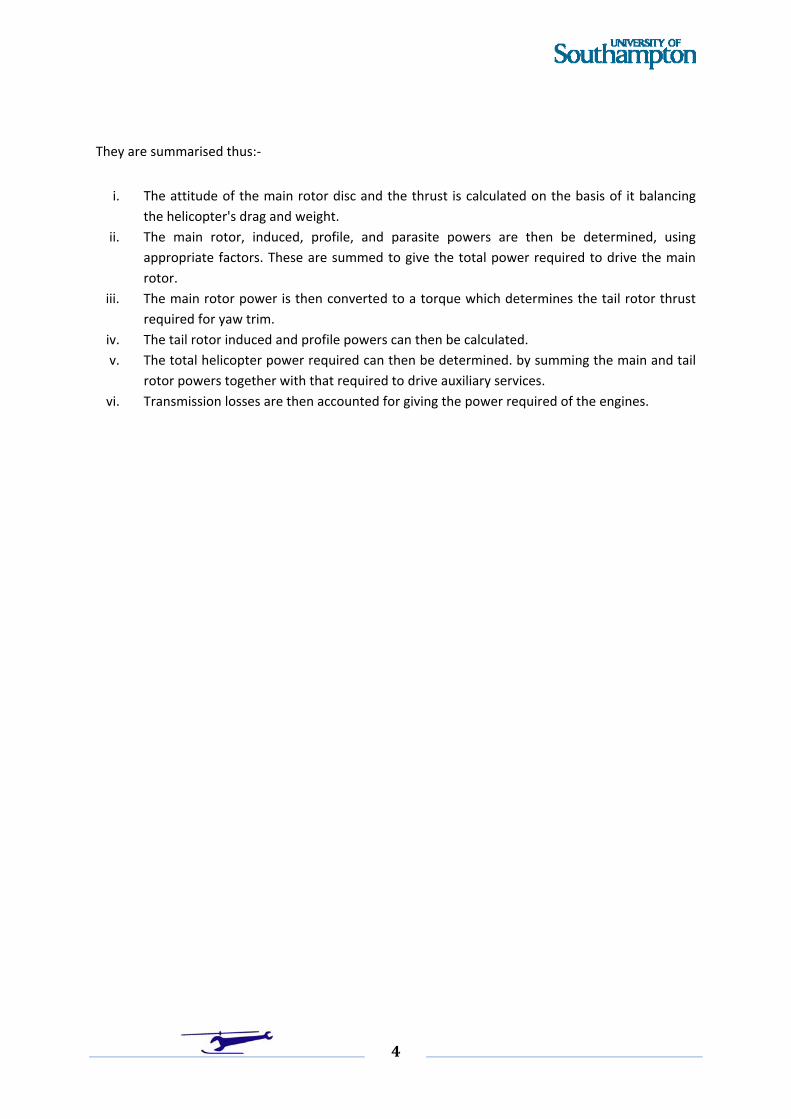
They are summarised thus:‐ 

i. The attitude of the main rotor disc and the thrust  is calculated on the basis of  it balancing 

the helicopter's drag and weight. 

ii. The  main  rotor,  induced,  profile,  and  parasite  powers  are  then  be  determined,  using 

appropriate factors. These are summed to give the total power required to drive the main 

rotor. 

iii. The main rotor power  is then converted to a torque which determines the tail rotor thrust 

required for yaw trim. 

iv. The tail rotor induced and profile powers can then be calculated. 

v. The total helicopter power required can then be determined. by summing the main and tail 

rotor powers together with that required to drive auxiliary services. 

vi. Transmission losses are then accounted for giving the power required of the engines.  

 

 

 

  

 

5

 

 

 

GLOSSARY OF TERMS The terminology used in the analysis is presented in the following glossary. 

ROTOR 

 

  MAIN TAIL 

Thrust  TM  TT 

Blockage Factor  BLOCKM  BLOCKT 

Tip Speed  VTM  VTT 

No.of Blades  N  n 

Blade Chord  C  c 

Rotor Radius  R  r 

Disc Tilt  γS   

Advance Ratio  μM  μT 

Advance Ratio 

Component Parallel to Disc μxM  μxT 

Advance Ratio 

Component Perpendicular to Disc μzM   

Downwash  λiM  λiT 

 

 

  

 

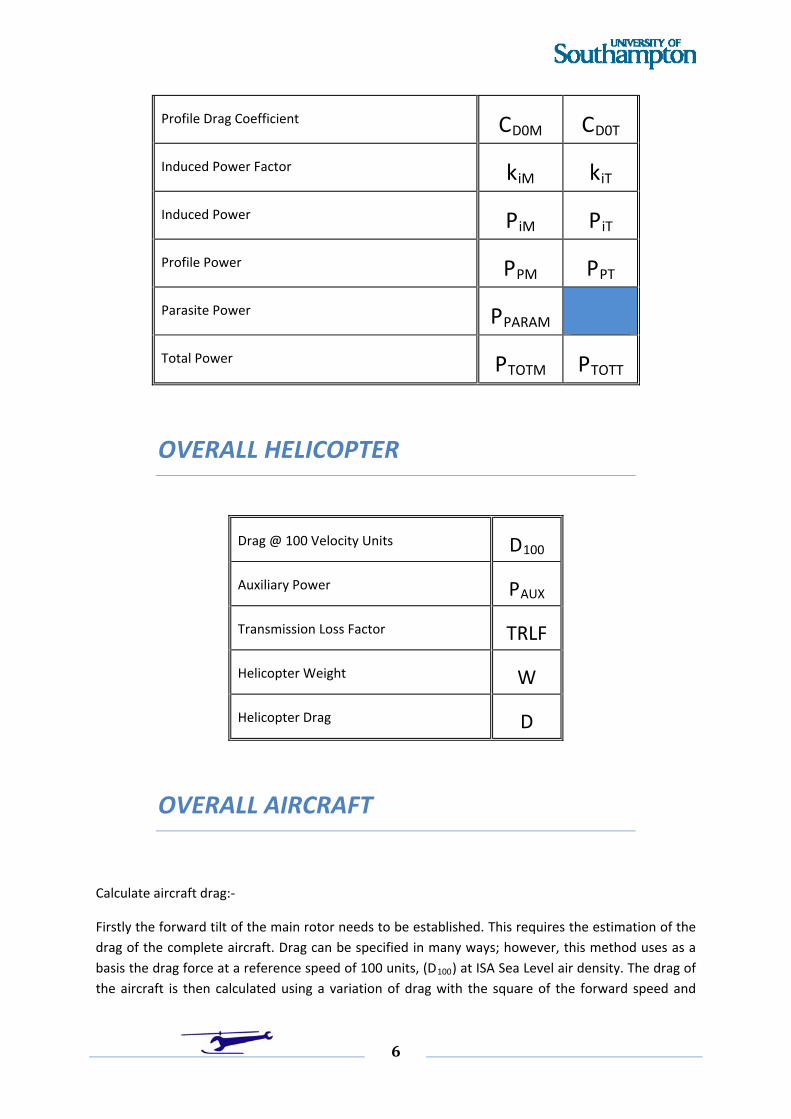
6

 

 

Profile Drag Coefficient  CD0M  CD0T 

Induced Power Factor  kiM  kiT 

Induced Power  PiM  PiT 

Profile Power  PPM  PPT 

Parasite Power  PPARAM   

Total Power  PTOTM  PTOTT 

 

OVERALL HELICOPTER 

 

Drag @ 100 Velocity Units  D100 

Auxiliary Power  PAUX 

Transmission Loss Factor  TRLF 

Helicopter Weight  W 

Helicopter Drag  D 

 

OVERALL AIRCRAFT 

 

Calculate aircraft drag:‐ 

Firstly the forward tilt of the main rotor needs to be established. This requires the estimation of the 

drag of the complete aircraft. Drag can be specified  in many ways; however, this method uses as a 

basis the drag force at a reference speed of 100 units, (D100) at ISA Sea Level air density. The drag of 

the aircraft  is  then calculated using a variation of drag with  the  square of  the  forward  speed and 

 

 

  

 

7

 

 

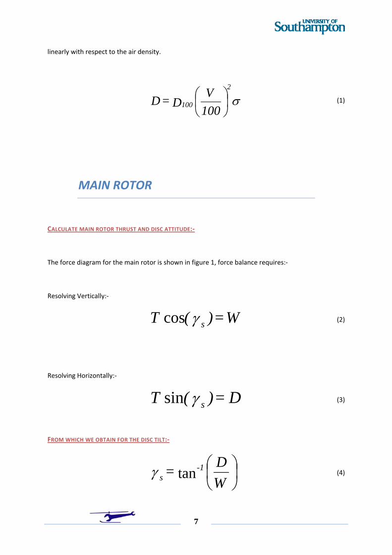
linearly with respect to the air density. 

 

 

100

V D = D

2

100  (1)

 

     

 

MAIN ROTOR 

 

CALCULATE MAIN ROTOR THRUST AND DISC ATTITUDE:‐ 

 

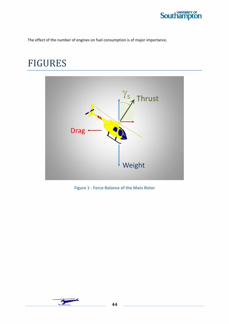
The force diagram for the main rotor is shown in figure 1, force balance requires:‐ 

 

Resolving Vertically:‐ 

  W = )( T scos (2)

 

     

Resolving Horizontally:‐ 

  D = )( T ssin 

(3)

     

FROM WHICH WE OBTAIN FOR THE DISC TILT:‐ 

 

W

D = 1-

s tan 

(4)

 

 

  

 

8

 

 

     

The main rotor thrust, with blockage, becomes:‐ 

 BLOCK D + W = T M

22 (5)

     

The blockage  term  is  applied  to  the main  rotor  thrust  as  a multiplying  factor  and  represents  the 

download on the fuselage due to the rotor downwash. 

 

The  induced velocity of  the main  rotor  is now  required. As actuator disc  theory  is  to be used,  the 

main  rotor advance  ratio  components parallel  to and normal  to  the  rotor disc plane are  required 

together with the thrust coefficient. 

 

The advance ratio is:‐ 

 

V

V =

TMM

 

(6)

     

Resolving parallel to the rotor disc:‐  

  sMxM = cos 

(7)

     

Resolving perpendicular to the rotor disc:‐ 

     

  sMzM = sin 

(8)

 

CALCULATE MAIN ROTOR DOWNWASH:‐ 

 

The main rotor downwash can now be calculated using the iterative technique. 

 

 

  

 

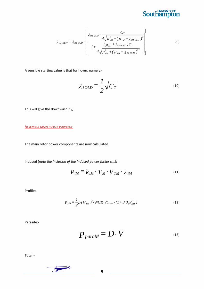
9

 

 

 

)+(+4

C)+(+1

)+(+4

C -

- =

2OLD iMzM

2xM

3TOLD iMzM

2OLD iMzM

2xM

TOLD iM

OLD iMNEW iM

 

(9)

     

A sensible starting value is that for hover, namely:‐ 

 

C2

1 = TOLD i

 

(10)

     

This will give the downwash λ iM. 

 

ASSEMBLE MAIN ROTOR POWERS:‐ 

 

The main rotor power components are now calculated. 

 

Induced (note the inclusion of the induced power factor kiM):‐ 

  iMTMMiMiM VTk= P (11)

     

Profile:‐ 

 )3.0+(1CNCR)V(

8

1 = P

2XMD0MTM

3pM   (12)

     

Parasite:‐ 

  VD = PparaM  

(13)

     

Total:‐ 

 

 

  

 

10

 

 

     

  P+P+P= P paraMpMiMTOTM 

(14)

 

It should be noted that in equations (12,19) the μx2 term is multiplied by 3.0. This is the value which 

was obtained in v.40. The extra effects raising this to 4.7 can be simply dealt with by amending the 

calculation method. 

 

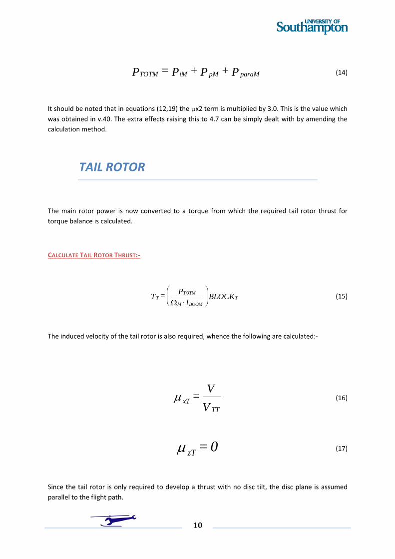
TAIL ROTOR 

 

The main  rotor power  is now converted  to a  torque  from which  the  required  tail  rotor  thrust  for 

torque balance is calculated. 

 

CALCULATE TAIL ROTOR THRUST:‐ 

     

 BLOCK

l P = T T

BOOMM

TOTMT

  (15)

 

The induced velocity of the tail rotor is also required, whence the following are calculated:‐ 

     

     

 

V

V =

TTxT

 

(16)

     

  0 = zT 

(17)

 

Since the tail rotor  is only required to develop a thrust with no disc tilt, the disc plane  is assumed 

parallel to the flight path. 

 

 

  

 

11

 

 

 

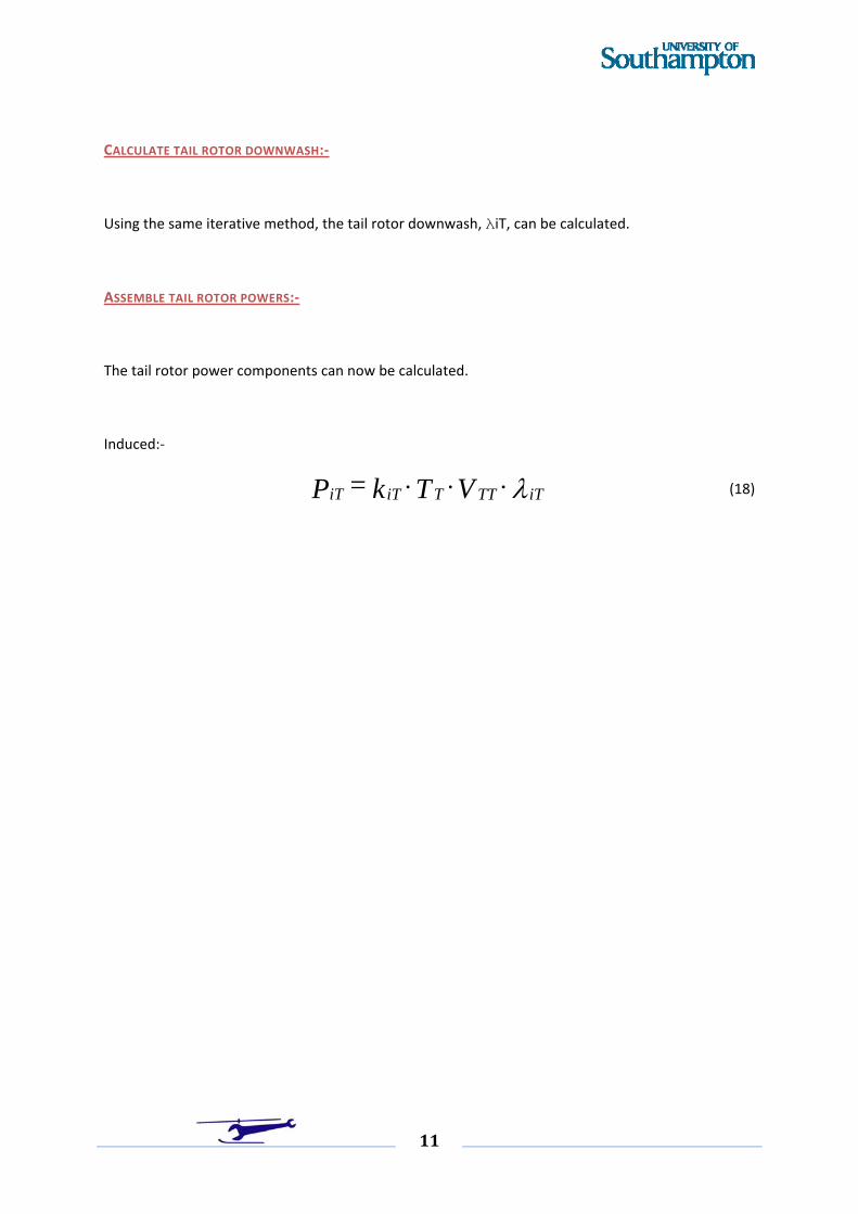
CALCULATE TAIL ROTOR DOWNWASH:‐ 

 

Using the same iterative method, the tail rotor downwash, λiT, can be calculated. 

 

ASSEMBLE TAIL ROTOR POWERS:‐ 

 

The tail rotor power components can now be calculated. 

 

Induced:‐ 

  iTTTTiTiT VTk= P (18)

     

 

 

  

 

12

 

 

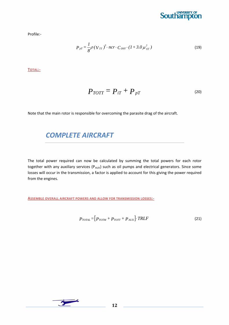
Profile:‐ 

 )3.0+(1Cncr)V(

8

1 = P

2XTD0TTT

3pT   (19)

     

TOTAL:‐ 

     

  P+P=P pTiTTOTT (20)

 

Note that the main rotor is responsible for overcoming the parasite drag of the aircraft. 

 

COMPLETE AIRCRAFT 

 

The  total  power  required  can  now  be  calculated  by  summing  the  total  powers  for  each  rotor 

together with any auxiliary services  (PAUX) such as oil pumps and electrical generators. Since some 

losses will occur in the transmission, a factor is applied to account for this giving the power required 

from the engines. 

 

ASSEMBLE OVERALL AIRCRAFT POWERS AND ALLOW FOR TRANSMISSION LOSSES:‐ 

     

  TRLF P + P + P = P AUXTOTTTOTMTOTAL (21)

 

 

 

  

 

13

 

 

 

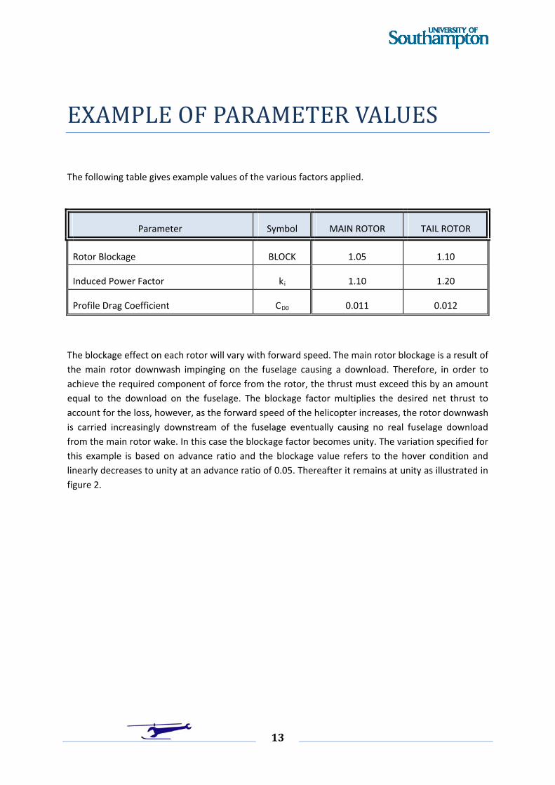
EXAMPLE OF PARAMETER VALUES  

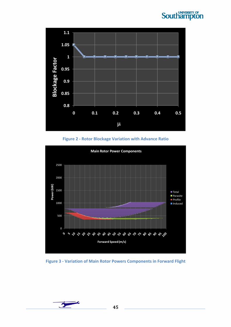
The following table gives example values of the various factors applied. 

 

Parameter  Symbol  MAIN ROTOR  TAIL ROTOR 

Rotor Blockage  BLOCK  1.05  1.10 

Induced Power Factor  ki  1.10  1.20 

Profile Drag Coefficient  CD0  0.011  0.012 

 

The blockage effect on each rotor will vary with forward speed. The main rotor blockage is a result of 

the main  rotor downwash  impinging  on  the  fuselage  causing  a download.  Therefore,  in order  to 

achieve the required component of force from the rotor, the thrust must exceed this by an amount 

equal  to  the  download  on  the  fuselage.  The  blockage  factor multiplies  the  desired  net  thrust  to 

account for the loss, however, as the forward speed of the helicopter increases, the rotor downwash 

is  carried  increasingly  downstream  of  the  fuselage  eventually  causing  no  real  fuselage  download 

from the main rotor wake. In this case the blockage factor becomes unity. The variation specified for 

this example  is based on advance  ratio and  the blockage value  refers  to  the hover  condition and 

linearly decreases to unity at an advance ratio of 0.05. Thereafter it remains at unity as illustrated in 

figure 2. 

 

 

  

 

14

 

 

CALCULATION OF ENGINE FUEL CONSUMPTION  

Having determined the power required from the engine(s) to fly a given helicopter flight condition, 

the fuel consumption can now be calculated. 

 

Engine fuel consumption data is often given in terms of specific fuel consumption (sfc) (kg/hr/kw) for 

a corresponding power setting  (P). A small conversion of  the data allows a very simple method of 

calculating the fuel consumption of a gas turbine engine developing a specified amount of power. 

 

The fuel flow of an engine (Wf) (kg/hr) can be obtained as the product of the sfc and the respective 

power. Plotting fuel flow against power produces a variation very close to linear and can be fitted by 

means  of  linear  regression  (least  squares).  Because  of  this  simple  linear  variation,  the  fuel 

consumption calculation becomes elementary. 

 

To enable full use to be made of the method, the operating altitude and temperature will need to be 

built in to the calculation. Each atmospheric condition will produce an individual straight line fit, but 

if the fuel flow and engine power are normalised by:‐ 

 

Where:‐     δ is the pressure ratio. 

      θ is the absolute temperature ratio. 

        (both relative to ISA Sea Level Atmosphere conditions.) 

 

the various  lines defining  the engine performance at a given atmospheric condition close together 

and the straight line law for the fuel flow becomes practically one line. 

 

i.e. The engine fuel consumption law for any atmospheric condition becomes:‐ 

 

P B + A =

WEE

f

 

(22)

 

 

  

 

15

 

 

     

This gives complete  flexibility as regards changing atmospheric conditions.  It should be noted  that 

this type of engine calculation assumes that the power unit is not operating close to a limit. 

 

The  straight  line  fit  possesses  a  positive  intercept  on  the  fuel  flow  axis  (AE) which  results  in  an 

important fact concerning the optimising of fuel consumption for a multi‐engined helicopter. 

 

Consider a helicopter which is fitted with N engines combining to give a total power production of P. 

Each engine must  then produce a power of P/N and the corresponding  fuel consumption  for all N 

engines is therefore:‐ 

 

1x

N

P B + A N =

WEE

f(23)

     

i.e.:‐ 

  P B + A N = W EEf   (24)

     

Because  of  the  first  term  of  the  right  hand  side  of  (24),  it  can  be  seen  that  for  a  given  power 

production,  a  smaller  number  of  engines  will  give  a  lower  fuel  consumption.  Consequently  a 

helicopter designer, when optimising for fuel consumption, will use a minimum number of engines 

capable of providing sufficient power. Other requirements such as helicopter performance with an 

engine failure tend to work in the opposite direction and, on this type of basis, the optimum design 

will  have  a maximum  number  of  engines. Hence,  choice  of  engine  for  a multi  engine  helicopter 

 thought. design is not as clear cut as might at first be

 

ENGINE LIMITS  

The previous discussions have considered the engine performance purely from a fuel consumption 

point of view.  In  reality, a gas  turbine engine will have  limitations which are usually based on  the 

permissible  operating  temperature  of  the  turbine  section. However,  it  is  possible  to  operate  the 

engine at higher power settings for a limited period of time without causing permanent damage. In 

emergency situations, some excessive power settings can be demanded for very limited time periods 

at the expense of accelerated engine wear or damage.  

 

 

  

 

16

 

 

Typical examples of power settings are described below:‐ 

 

Maximum Continuous Power Rating 

 

This is the maximum power that an engine can develop without a time constraint, and consequently 

operate continuously. 

 

Take Off or 1 Hour Power Rating 

 

This  is  used  for  the  higher  power  conditions  such  as  take  off  and  hover  at  high  altitude  and/or 

ambient temperature. It can be used for periods of approximately 1 hour (sometimes ½ hour) before 

the power demand must be reduced. 

 

Maximum Contingency or 2½ Minute 

Power Rating 

 

This is used with engine loss and other contingency situations when the power can be used for short 

periods of 2 to 3 minutes. 

 

An engine inspection after such use is usually considered. 

 

Emergency or ½ Minute Power Rating 

  

This  is  the highest and consequently  the most damaging condition.  It  is used  for situations where 

loss of the aircraft is a real possibility. 

 

 

 

  

 

17

 

 

An example is when a twin‐engined naval helicopter suffers an engine loss in a high power condition, 

(high all up weight and  in  the hover), and  is  forced  to ditch  in  the  sea. After  jettisoning as much 

weight as possible, a take off on a single engine from the water will be necessary to save the aircraft. 

Emergency power will be required for such a dire emergency and the engine will probably require 

extensive maintenance and refurbishment, if not scrapping, due to the use of such an excessive but 

necessary power demand. 

 

CALCULATION OF THE PERFORMANCE OF A HELICOPTER  

To  illustrate  the  method,  the  following  calculations,  based  on  a  small  utility  helicopter  are 

presented. 

 

The input data required is shown below:‐ 

 

Rotor Data  Main Rotor  Tail Rotor 

No. of Blades  4  4 

Chord (m)  0.394  0.180 

Radius (m)  6.4  1.105 

Tip Speed (m/s)  218.69  218.69 

Blockage  1.05  1.10 

Induced Power Factor (ki)  1.10  1.20 

Profile  Drag  Coefficient 

(CD0) 

0.011  0.012 

 

 

Fuselage Data 

Tail Boom Length (m)  7.66 

 

 

  

 

18

 

 

D100 (N)  6226.9 

Auxiliary Power PAUX (kw)  26.1 

Transmission Loss Factor (TRLF)  1.04 

 

 

  

 

19

 

 

No. of Engines = 2 

 

The  fuel  flow  law,  presented  in  (25), was  obtained  from  public  domain  information  using  linear 

regression:‐ 

 

P

0.24 + 46.5 = W f

 

(25)

     

With  the  above  data,  the  variation  of  the main  rotor  power  components with  forward  speed  is 

shown in figure 3, namely induced, profile, parasite, and total. 

 

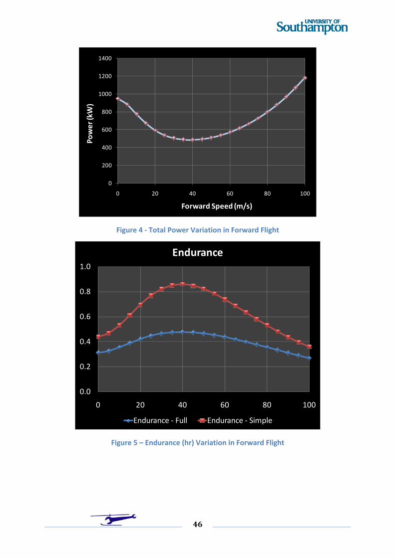
It is instructive to see these results when shown cumulatively as in figure 4, 

The  following are  then added  to  the main  rotor power,  tail  rotor power, auxiliary power, and  the 

influence of transmission losses to give the total overall power required of the powerplants. 

 

The total power variation of the complete helicopter with forward speed is shown in figure 5. 

 

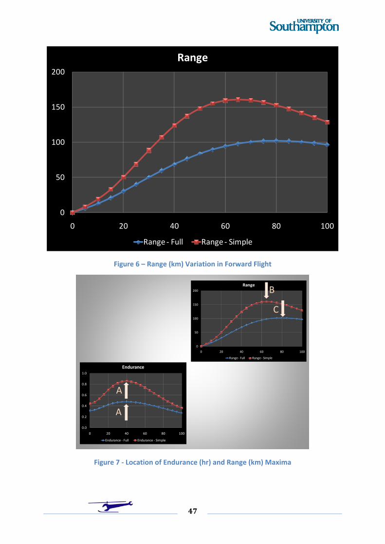
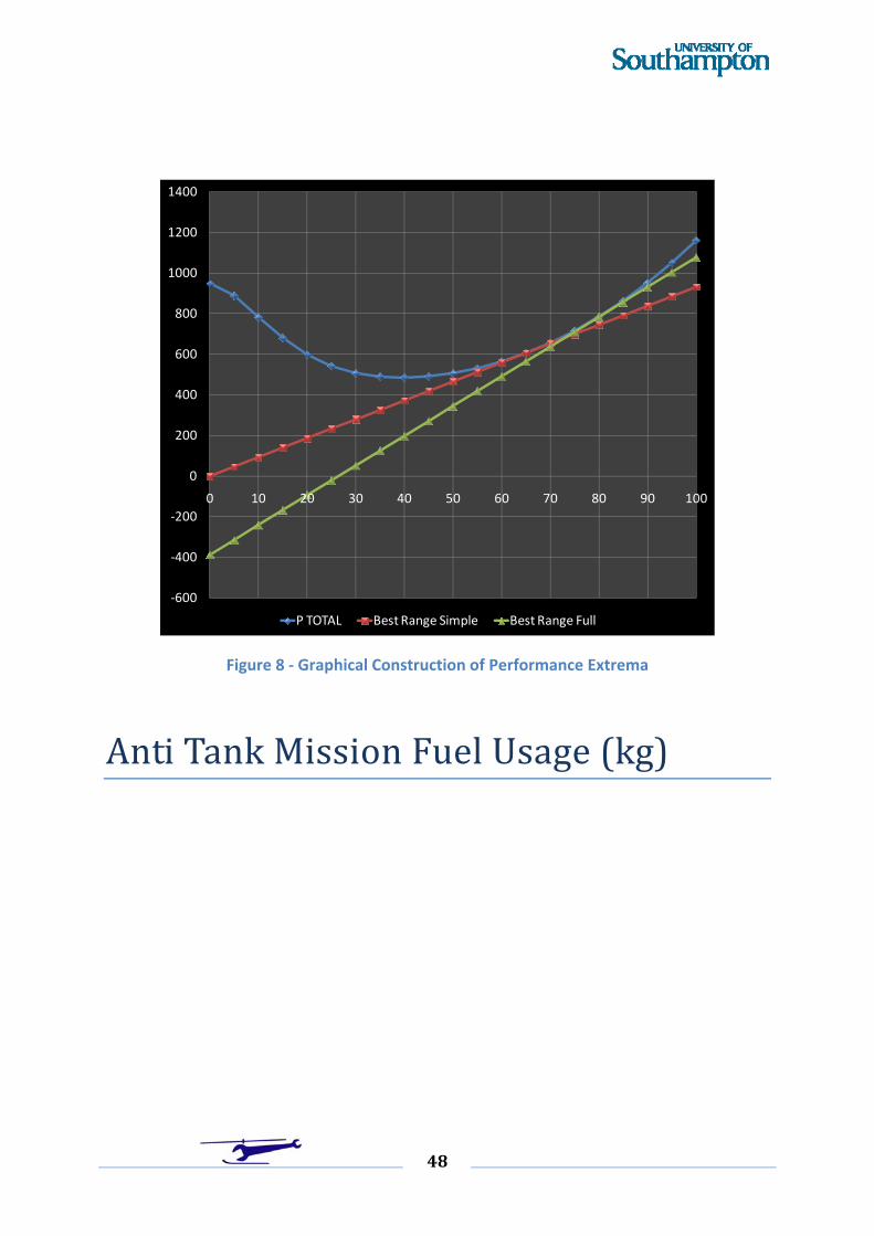
From this power distribution the fuel flow can now be calculated and converted to endurance and 

range estimates. Endurance is the time required to consume a specified amount of fuel, whilst range 

is the corresponding distance covered. Endurance  is concerned principally with minimising the rate 

of  fuel usage with  time, whilst  range  is  a  compromise between  time  and  forward  speed.  (A  fuel 

usage of 100 kg is assumed for these calculations.) The endurance is shown in figure 6, and the range 

(km) is shown in figure 7. Two plots are presented in each figure corresponding to the full fuel flow 

law defined in equation (1), and a modified law where the intercept (AE, or fuel flow at zero power) 

is set to zero. (This corresponds to a constant sfc.) The lower curve corresponds to the full law (AE0) and the upper curve to the modified law (AE=0). 

 

The  positions  of maximum  endurance  and  range  are  indicated  in  the  figures.  As  can  be  seen, 

changing  the  fuel  flow  law  does  not  alter  the  optimum  endurance  speed  of  38 m/s  (A), which 

corresponds  to minimum  power.  However,  the  change  does  have  an  influence  on  the  optimum 

range speed increasing it from 65 m/s (B) to 80 m/s (C). 

Figure 8 shows the three extrema indicated by A, B, and C on the total power v forward speed curve. 

 

 

 

  

 

20

 

 

In  fact,  the  three  points  A,  B,  and  C,  corresponding  to  the  various  extrema,  can  be  determined 

geometrically as the following analysis shows, using the following definitions:‐ 

 

  WFUEL  = Fuel Weight (fixed) 

  T  = Time 

  S  = sfc 

  P  = Power 

  V  = Forward Speed 

  E  = Endurance 

  R  = Range 

 

we have the following:‐ 

 

Point A (maximum endurance) 

 

The definition for sfc is :‐ 

 

TPW = S FUEL

 

(26)

     

i.e.:‐ 

 

P

1

SW = T FUEL

 (27)

     

As WFUEL and S are fixed, T is maximum when P is minimum, i.e. point A is the minimum point on the 

Power v Velocity curve. 

 

 

 

  

 

21

 

 

Point B (maximum range ‐ constant sfc, AE=0) 

 

The range is given by:‐ 

 

SW

P

V =

VT = R

FUEL

 

(28)

     

i.e. R is a maximum when P/V is a minimum, so point B is positioned where the tangent, drawn from 

the origin, touches the power curve. 

 

Point C (maximum range ‐ full fuel flow law) 

 

For this case we have:‐ 

  P B + A T = W EEFUEL   (29)

     

Therefore:‐ 

 

P + B

A

V

B

W =

WP B + A

V =

TV = R

E

EE

FUEL

FUELEE

 

(30)

     

This  is very similar  to point B except  that  the additional  term  in  the denominator  (AE/BE) requires 

that the tangent be drawn from the point (0,‐AE/BE). The construction for the three points is shown 

in figure 9. 

Wind 

If the helicopter is flying into a headwind of VW, the above formula for range becomes: 

 

 

  

 

22

 

 

 

P + B

A

VV

B

W =

WP B + A

VV =

TVV = R

E

E

W

E

FUEL

FUELEE

W

W

 

(31)

This means that the tangent should be drawn from the point (VW,‐AE/BE). 

 

 

  

 

23

 

 

MISSION ANALYSIS  

The  calculation  of  engine  power  and  fuel  consumption  can  be  extended  to  "fly"  a mission  in  a 

computer which  is of direct use to a project assessment.  In  flying a mission, the helicopter weight 

will be changing due to fuel usage consequently this must be accounted for  in the calculations and 

the method described here uses a technique which  is simple to  implement. The mission  is divided 

into legs, each being calculated separately, in sequence, with the value of the aircraft weight at the 

end of a particular leg becoming the start value for the succeeding leg. (Each leg will describe a fixed 

flight condition, particularly altitude and/or forward speed.) This also allows discrete weight changes 

of payload  to be  incorporated,  such as changes  in passenger/cargo payload or  the deployment of 

ordnance.  

 

For each leg the power and fuel consumption at the start weight is calculated. Knowing the duration 

of the  leg a first estimate of the weight change over the  leg  is obtained. Taking the mean value of 

aircraft weight the process is repeated and the fuel usage of the leg at the two weights compared. If 

they lie within a specified tolerance, the final estimate is taken. If not, a revised mean aircraft weight 

is adopted (using the latest fuel usage figure) and the process repeated iteratively until convergence 

to within the required tolerance is achieved. 

 

CALCULATION METHOD  

A summary of the calculation method  is presented and can be used as a basis  for a  flow diagram. 

Each part of the calculation is presented as a complete entity with the input and output data being 

specified.  This  imparts  a  segmented  structure  to  the  method  which  is  recommended  for 

implementation in a computer program. 

 

ATMOSPHERIC PARAMETERS 

 

This allows  the air characteristics  required by  the calculations  to be determined  from  the altitude 

and ambient temperature. 

 

 

 

  

 

24

 

 

The helicopter is assumed to remain within the troposphere. 

 

Input 

 

Altitude, 

Sea Level Air Temperature, 

Sea Level Air Density. 

Output 

 

Density Ratio (σ), 

Absolute Temperature Ratio (θ), 

Pressure Ratio (δ). 

 

Calculation 

 

The absolute temperature ratio is given by:‐ 

     

 

T

LapseRate*Altitude - T = SeaLevel

SeaLevel (32)

 

The pressure ratio by:‐ 

     

 

5.256 =  

(33)

 

 

  

 

25

 

 

 

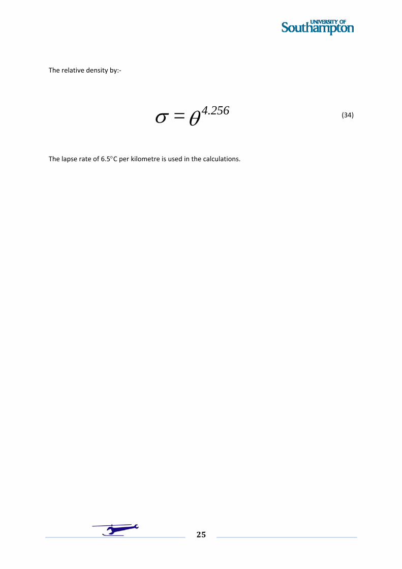
The relative density by:‐ 

     

 

4.256 =  

(34)

 

The lapse rate of 6.5C per kilometre is used in the calculations. 

 

 

  

 

26

 

 

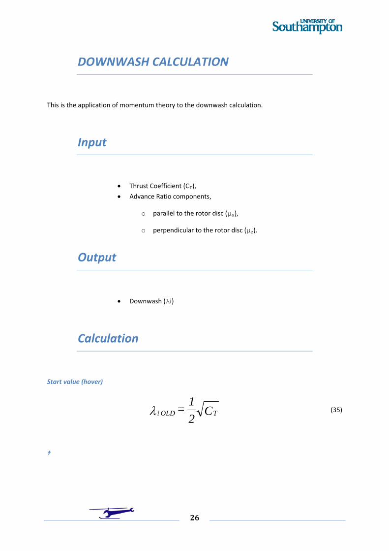
DOWNWASH CALCULATION 

 

This is the application of momentum theory to the downwash calculation. 

 

Input 

 

Thrust Coefficient (CT), 

Advance Ratio components, 

o parallel to the rotor disc (μx), 

o perpendicular to the rotor disc (μz). 

Output 

 

Downwash (λi) 

 

Calculation 

 

Start value (hover) 

 

C2

= TOLD i1

 

(35)

     

† 

 

 

  

 

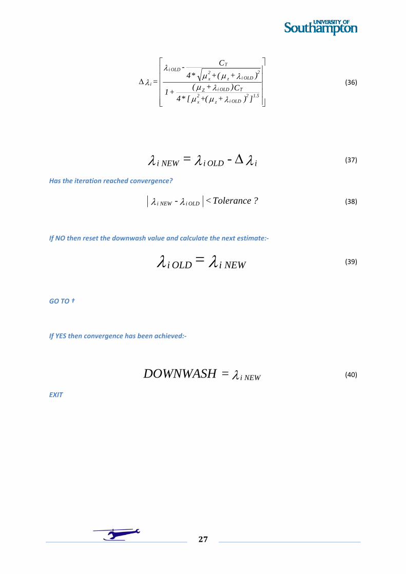
27

 

 

 

])+(+[*4C)+(

+ 1

)+(+*4

C-

=

1.52OLD iz

2x

TOLD iZ

OLD iz22

x

TOLD i

i

(36)

     

     

  iOLD iNEW i - = (37)

Has the iteration reached convergence? 

  ? Tolerance < - OLD iNEW i (38)

     

If NO then reset the downwash value and calculate the next estimate:‐ 

  NEW iOLD i = 

(39)

     

GO TO † 

 

If YES then convergence has been achieved:‐ 

     

  NEW i = DOWNWASH (40)

EXIT  

 

 

  

 

28

 

 

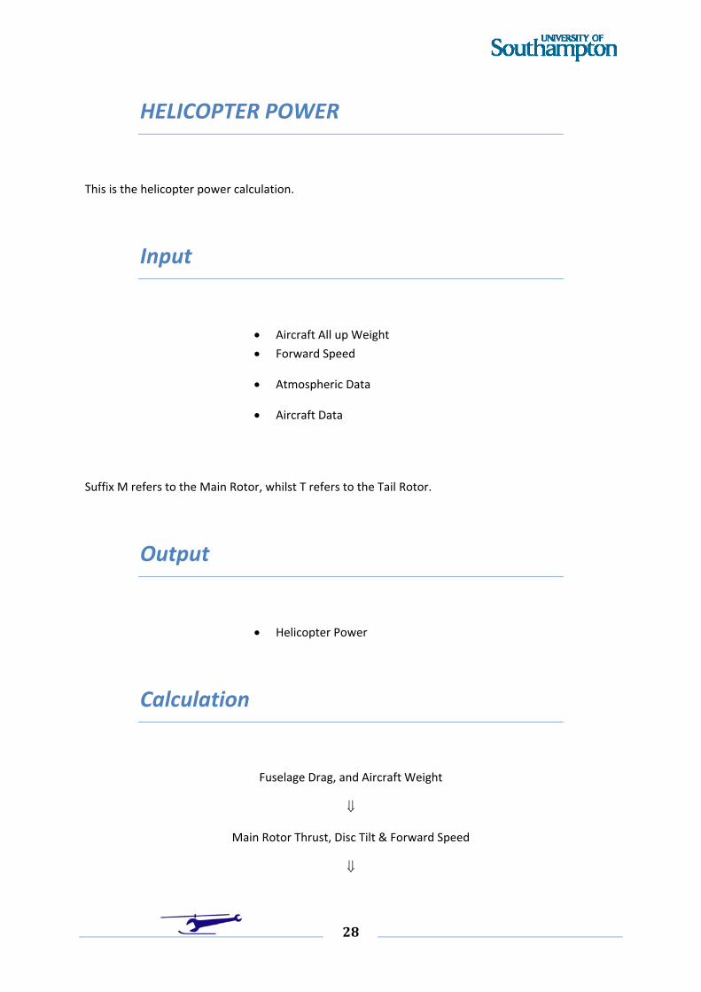
HELICOPTER POWER 

 

This is the helicopter power calculation. 

 

Input 

 

Aircraft All up Weight 

Forward Speed 

Atmospheric Data 

Aircraft Data 

 

Suffix M refers to the Main Rotor, whilst T refers to the Tail Rotor. 

 

Output 

 

Helicopter Power 

 

Calculation 

 

Fuselage Drag, and Aircraft Weight 

 

Main Rotor Thrust, Disc Tilt & Forward Speed 

 

 

 

  

 

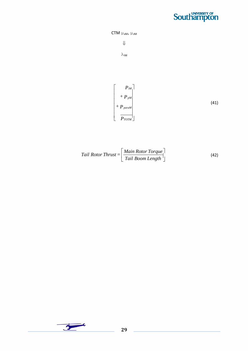
29

 

 

CTM μxM, μzM 

 

λ iM 

 

   

 

P

P +

P +

P

TOTM

paraM

pM

iM

 

(41)

   

     

 

Length Boom Tail

Torque Rotor Main = Thrust Rotor Tail (42)

 

 

  

 

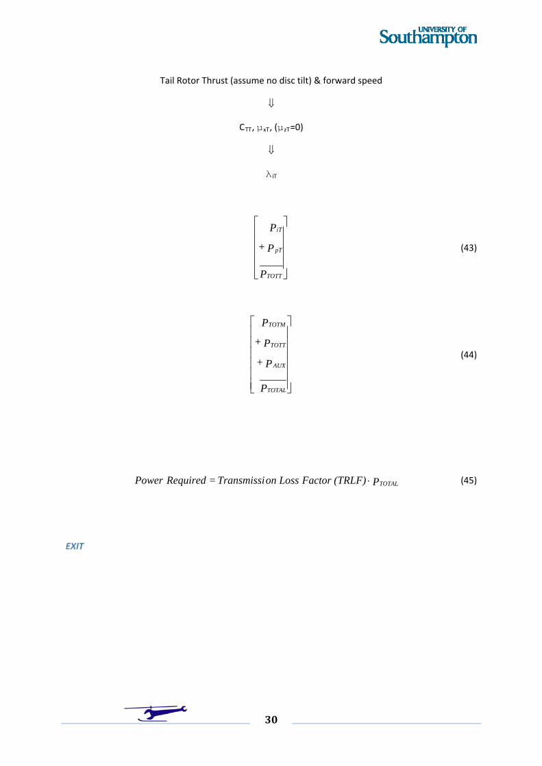
30

 

 

Tail Rotor Thrust (assume no disc tilt) & forward speed 

 

CTT, μxT, (μzT=0) 

 

λ iT 

 

 

P

P +

P

TOTT

pT

iT

 

(43)

     

 

P

P +

P +

P

TOTAL

AUX

TOTT

TOTM

 

(44)

     

 

     

  P (TRLF) Factor Loss onTransmissi = Required Power TOTAL   (45)

 

EXIT 

 

 

  

 

31

 

 

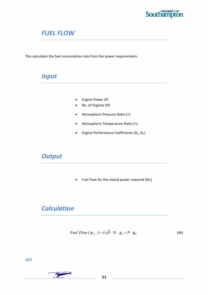
FUEL FLOW 

 

This calculates the fuel consumption rate from the power requirements. 

 

Input 

 

Engine Power (P) 

No. of Engines (N) 

Atmospheric Pressure Ratio (δ) 

Atmospheric Temperature Ratio (θ) 

Engine Performance Coefficients (AE, BE) 

 

Output 

 

Fuel Flow for the stated power required (Wf) 

 

 

Calculation 

     

  B P + A N = ) W( Flow Fuel EEf (46)

 

 

EXIT 

 

 

  

 

32

 

 

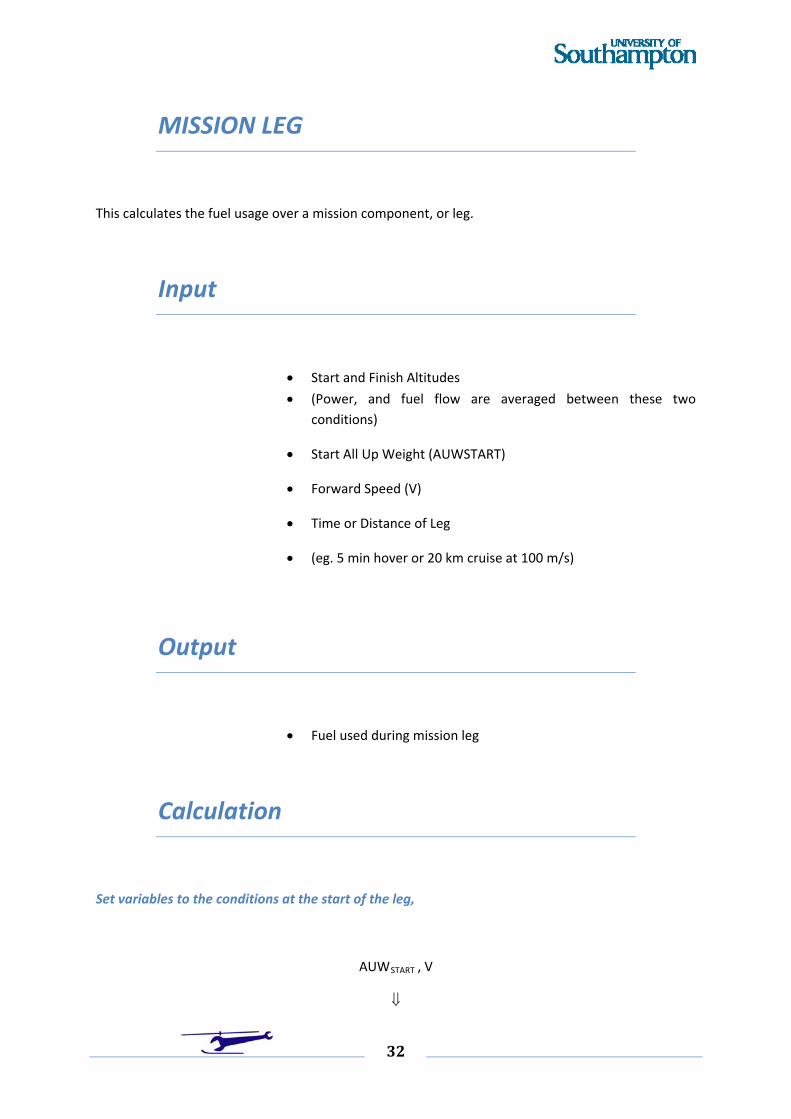
MISSION LEG 

 

This calculates the fuel usage over a mission component, or leg. 

 

Input 

 

Start and Finish Altitudes 

(Power,  and  fuel  flow  are  averaged  between  these  two 

conditions) 

Start All Up Weight (AUWSTART) 

Forward Speed (V) 

Time or Distance of Leg 

(eg. 5 min hover or 20 km cruise at 100 m/s) 

 

Output 

 

Fuel used during mission leg 

 

Calculation 

 

Set variables to the conditions at the start of the leg, 

 

AUWSTART , V 

 

 

 

  

 

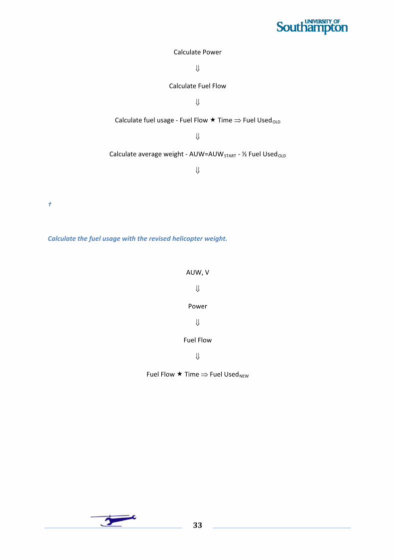
33

 

 

Calculate Power 

 

Calculate Fuel Flow 

 

Calculate fuel usage ‐ Fuel Flow  Time  Fuel UsedOLD 

 

Calculate average weight ‐ AUW=AUWSTART ‐ ½ Fuel UsedOLD 

 

 

† 

 

Calculate the fuel usage with the revised helicopter weight. 

 

AUW, V 

 

Power 

 

Fuel Flow 

 

Fuel Flow  Time  Fuel UsedNEW 

 

 

  

 

34

 

 

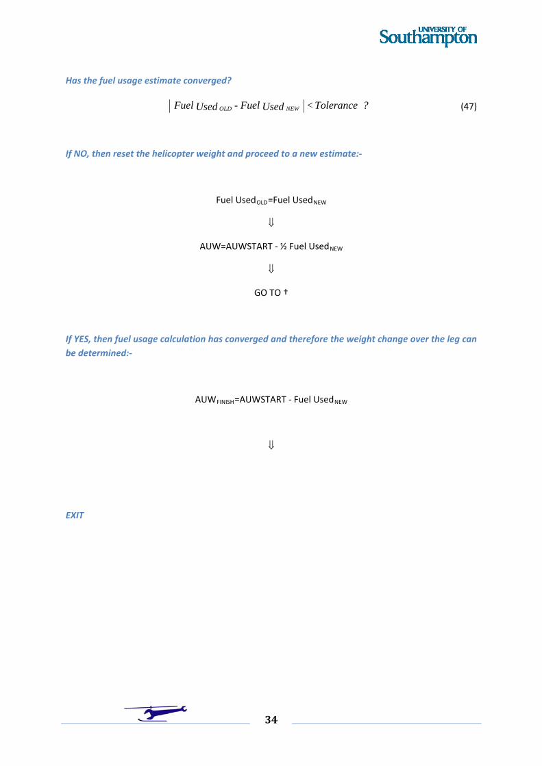
Has the fuel usage estimate converged? 

  ? Tolerance < Used Fuel - Used Fuel NEWOLD (47)

     

If NO, then reset the helicopter weight and proceed to a new estimate:‐ 

 

Fuel UsedOLD=Fuel UsedNEW 

 

AUW=AUWSTART ‐ ½ Fuel UsedNEW 

 

GO TO † 

 

If YES, then fuel usage calculation has converged and therefore the weight change over the leg can 

be determined:‐ 

 

AUWFINISH=AUWSTART ‐ Fuel UsedNEW 

 

 

 

 

EXIT 

 

 

  

 

35

 

 

EXAMPLES OF MISSION CALCULATIONS  

To see the application of the calculation to a mission, two examples are presented here. They are for 

the WG13 aircraft flying:‐ 

 

i. A mission performed mainly at high speed, such as anti‐tank. 

ii. A mission containing much hover time, such as anti‐submarine (ASW). 

 

They do not represent existing missions but are used merely to examine the performance of a given 

helicopter engaged on missions which contain either significant elements of high speed operation or 

hover time. 

 

The mission calculation was performed using the Westland WG13/Lynx as a datum aircraft for five 

helicopter designs, each  illustrating the type of parametric change which a designer could choose. 

The results show the effect of such changes on the fuel usage of the Lynx aircraft. 

 

Case 1  This is the basic aircraft. 

 

Case 2  This has the aircraft parasitic drag doubled via the D100 term. 

 

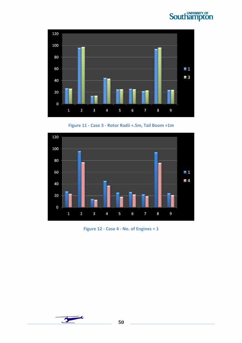
Case 3  This has the main and tail rotor radii increased by 0.5 m, with the consequent increase in tail 

boom length of 1 m. 

 

Case 4  The number of engines are reduced to 1. No allowance has been made for the ability of the 

single engine to generate sufficient power. Only the fuel consumption has been studied. 

 

Case 5  The number of engines are  increased to 3. The data used  for the power calculation of the 

Westland Lynx is used as a basis for these calculations. 

 

 

  

 

36

 

 

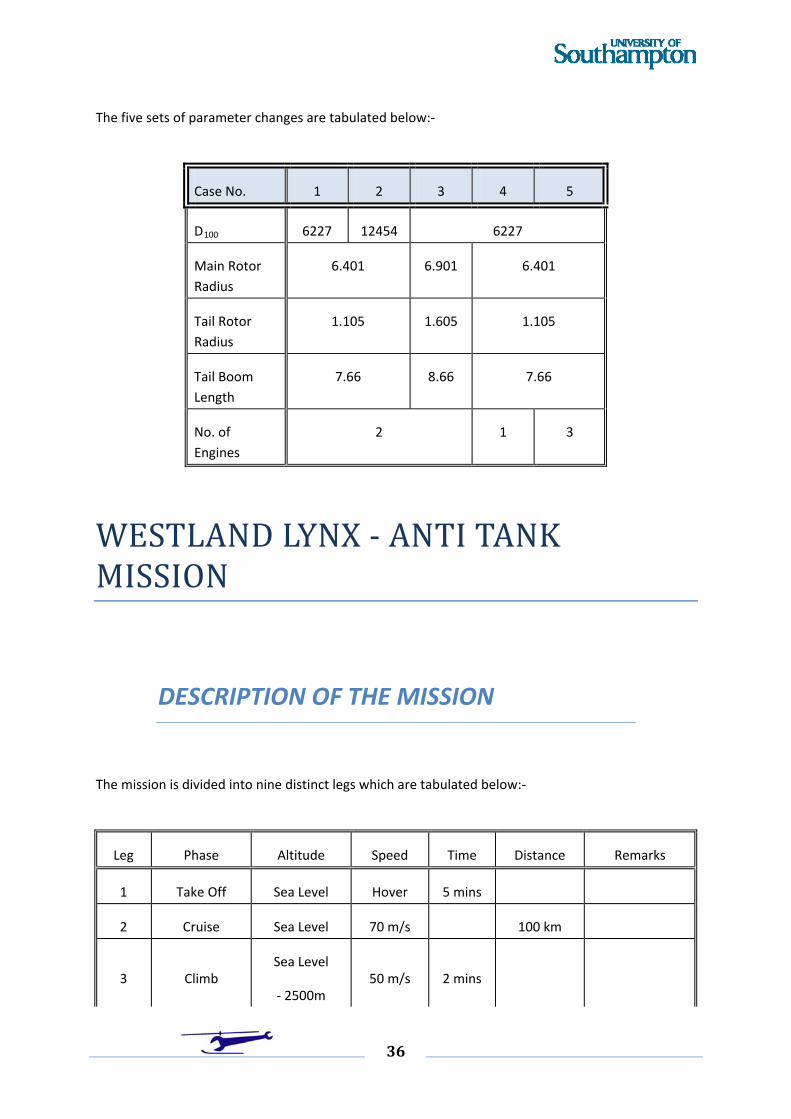
The five sets of parameter changes are tabulated below:‐ 

 

Case No.  1  2  3  4  5 

D100  6227  12454  6227 

Main Rotor 

Radius 

6.401  6.901  6.401 

Tail Rotor 

Radius 

1.105  1.605  1.105 

Tail Boom 

Length 

7.66  8.66  7.66 

No. of 

Engines 

2  1  3 

 

WESTLAND LYNX ‐ ANTI TANK MISSION 

 

DESCRIPTION OF THE MISSION 

 

The mission is divided into nine distinct legs which are tabulated below:‐ 

 

Leg  Phase  Altitude  Speed  Time  Distance  Remarks 

1  Take Off  Sea Level  Hover  5 mins     

2  Cruise  Sea Level  70 m/s    100 km   

3  Climb Sea Level 

‐ 2500m 50 m/s  2 mins   

 

 

 

  

 

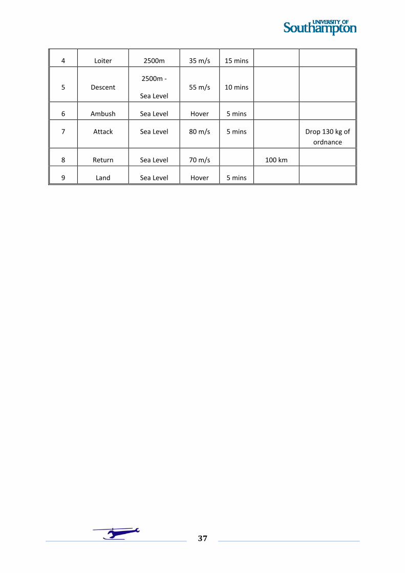
37

 

 

4  Loiter  2500m  35 m/s  15 mins     

5  Descent 2500m ‐ 

Sea Level 55 m/s  10 mins   

 

6  Ambush  Sea Level  Hover  5 mins     

7  Attack  Sea Level  80 m/s  5 mins    Drop 130 kg of 

ordnance 

8  Return  Sea Level  70 m/s    100 km   

9  Land  Sea Level  Hover  5 mins     

 

 

  

 

38

 

 

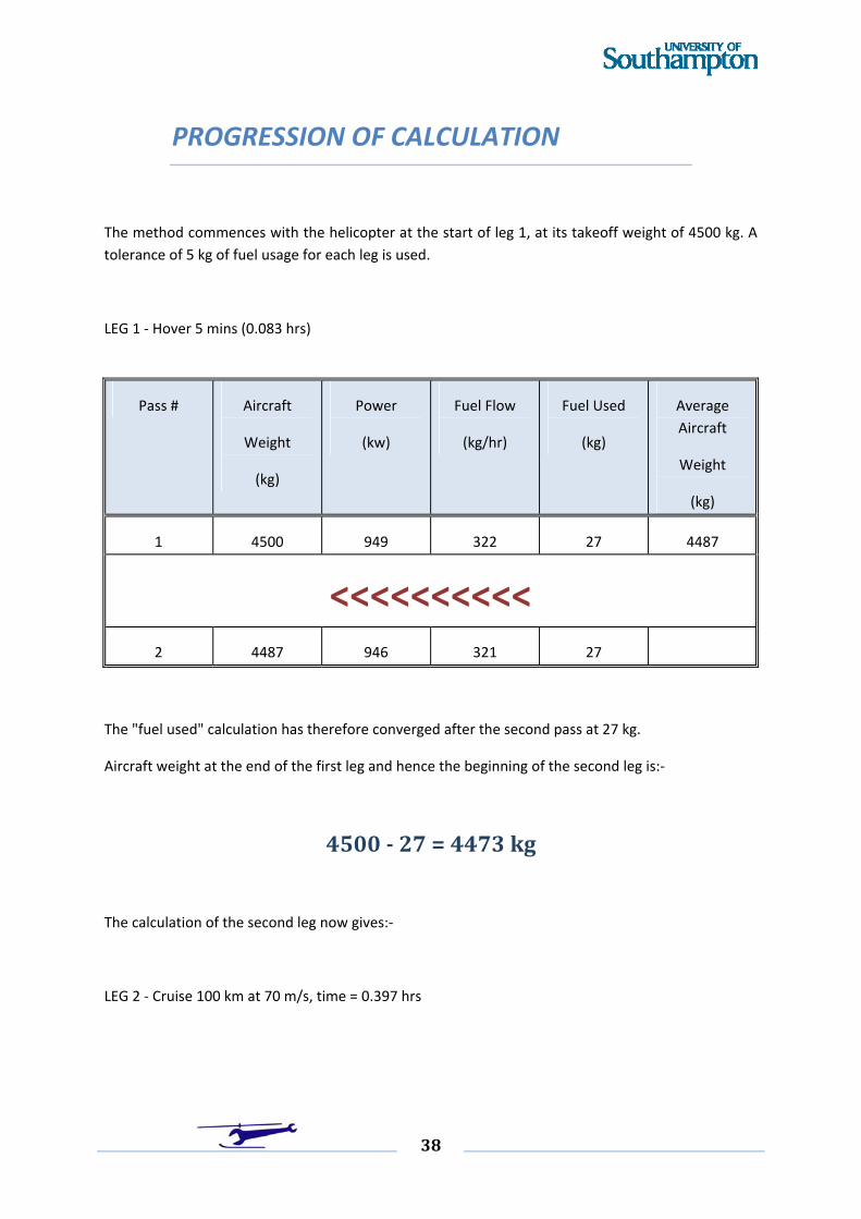
PROGRESSION OF CALCULATION 

 

The method commences with the helicopter at the start of leg 1, at its takeoff weight of 4500 kg. A 

tolerance of 5 kg of fuel usage for each leg is used. 

 

LEG 1 ‐ Hover 5 mins (0.083 hrs) 

 

Pass #  Aircraft 

Weight 

(kg) 

Power 

(kw) 

Fuel Flow 

(kg/hr) 

Fuel Used 

(kg) 

Average 

Aircraft 

Weight 

(kg) 

1  4500  949  322  27  4487 

<<<<<<<<<< 2  4487  946  321  27   

 

The "fuel used" calculation has therefore converged after the second pass at 27 kg. 

Aircraft weight at the end of the first leg and hence the beginning of the second leg is:‐ 

 

4500 ­ 27 = 4473 kg 

 

The calculation of the second leg now gives:‐ 

 

LEG 2 ‐ Cruise 100 km at 70 m/s, time = 0.397 hrs 

 

 

 

  

 

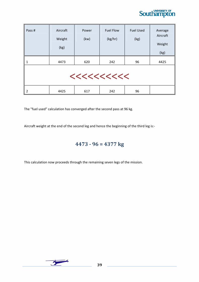
39

 

 

Pass #  Aircraft 

Weight 

(kg) 

Power 

(kw) 

Fuel Flow 

(kg/hr) 

Fuel Used 

(kg) 

Average 

Aircraft 

Weight 

(kg) 

1  4473  620  242  96  4425 

<<<<<<<<<< 

2  4425  617  242  96   

 

The "fuel used" calculation has converged after the second pass at 96 kg. 

 

Aircraft weight at the end of the second leg and hence the beginning of the third leg is:‐ 

 

4473 ­ 96 = 4377 kg 

 

This calculation now proceeds through the remaining seven legs of the mission. 

 

 

 

  

 

40

 

 

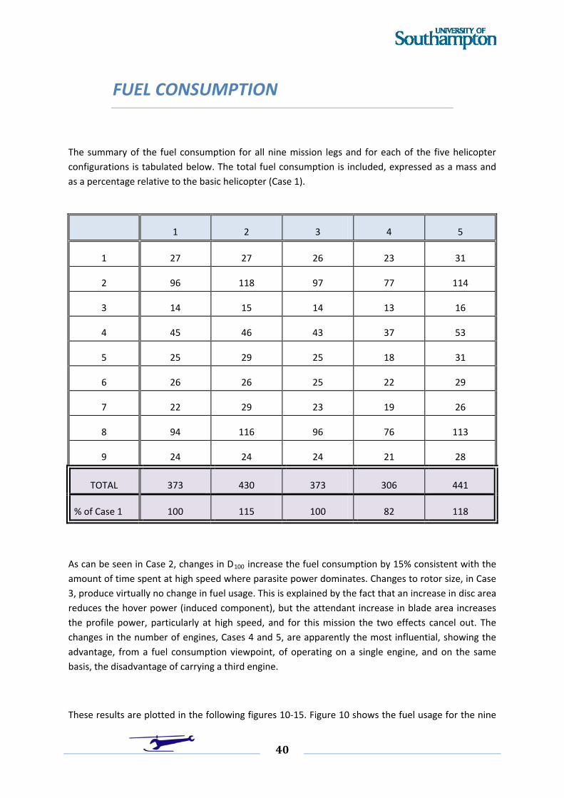
FUEL CONSUMPTION 

 

The summary of  the  fuel consumption  for all nine mission  legs and  for each of  the  five helicopter 

configurations  is tabulated below. The total fuel consumption  is  included, expressed as a mass and 

as a percentage relative to the basic helicopter (Case 1). 

 

  1  2  3  4  5 

1  27  27  26  23  31 

2  96  118  97  77  114 

3  14  15  14  13  16 

4  45  46  43  37  53 

5  25  29  25  18  31 

6  26  26  25  22  29 

7  22  29  23  19  26 

8  94  116  96  76  113 

9  24  24  24  21  28 

TOTAL  373  430  373  306  441 

% of Case 1  100  115  100  82  118 

 

As can be seen in Case 2, changes in D100 increase the fuel consumption by 15% consistent with the 

amount of time spent at high speed where parasite power dominates. Changes to rotor size, in Case 

3, produce virtually no change in fuel usage. This is explained by the fact that an increase in disc area 

reduces the hover power (induced component), but the attendant  increase  in blade area  increases 

the profile power, particularly at high  speed, and  for  this mission  the  two effects cancel out. The 

changes  in the number of engines, Cases 4 and 5, are apparently the most  influential, showing the 

advantage,  from a  fuel consumption viewpoint, of operating on a  single engine, and on  the  same 

basis, the disadvantage of carrying a third engine. 

 

These results are plotted in the following figures 10‐15. Figure 10 shows the fuel usage for the nine 

 

 

  

 

41

 

 

legs and under each leg, the five helicopter configurations. Figures 11‐15 show the helicopter weight 

variation with time for each configuration over the complete mission. 

 

 

  

 

42

 

 

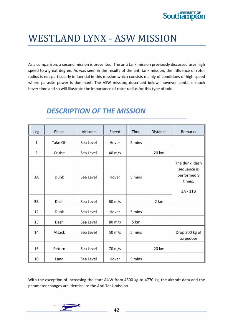
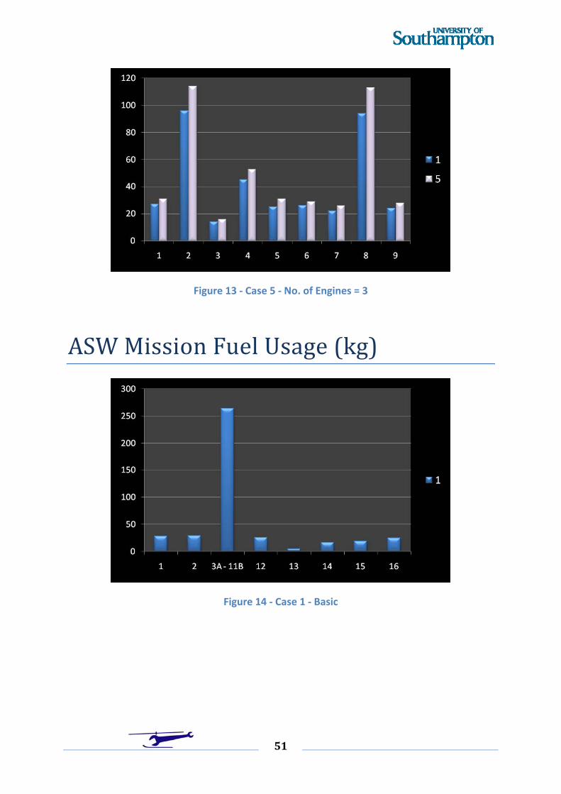
WESTLAND LYNX ‐ ASW MISSION  

As a comparison, a second mission is presented. The anti tank mission previously discussed uses high 

speed to a great degree. As was seen  in the results of the anti tank mission, the  influence of rotor 

radius is not particularly influential in this mission which consists mainly of conditions of high speed 

where  parasite  power  is  dominant.  The  ASW mission,  described  below,  however  contains much 

hover time and so will illustrate the importance of rotor radius for this type of role. 

 

DESCRIPTION OF THE MISSION 

Leg  Phase  Altitude  Speed  Time  Distance  Remarks 

1  Take Off  Sea Level  Hover  5 mins     

2  Cruise  Sea Level  40 m/s    20 km   

3A  Dunk  Sea Level  Hover  5 mins 

  The dunk, dash 

sequence is 

performed 9 

times. 

3A ‐ 11B 

3B  Dash  Sea Level  60 m/s    2 km   

12  Dunk  Sea Level  Hover  5 mins     

13  Dash  Sea Level  80 m/s  5 km     

14  Attack  Sea Level  50 m/s  5 mins    Drop 300 kg of 

torpedoes 

15  Return  Sea Level  70 m/s    20 km   

16  Land  Sea Level  Hover  5 mins     

 

With the exception of  increasing the start AUW from 4500 kg to 4770 kg, the aircraft data and the 

parameter changes are identical to the Anti Tank mission. 

 

 

  

 

43

 

 

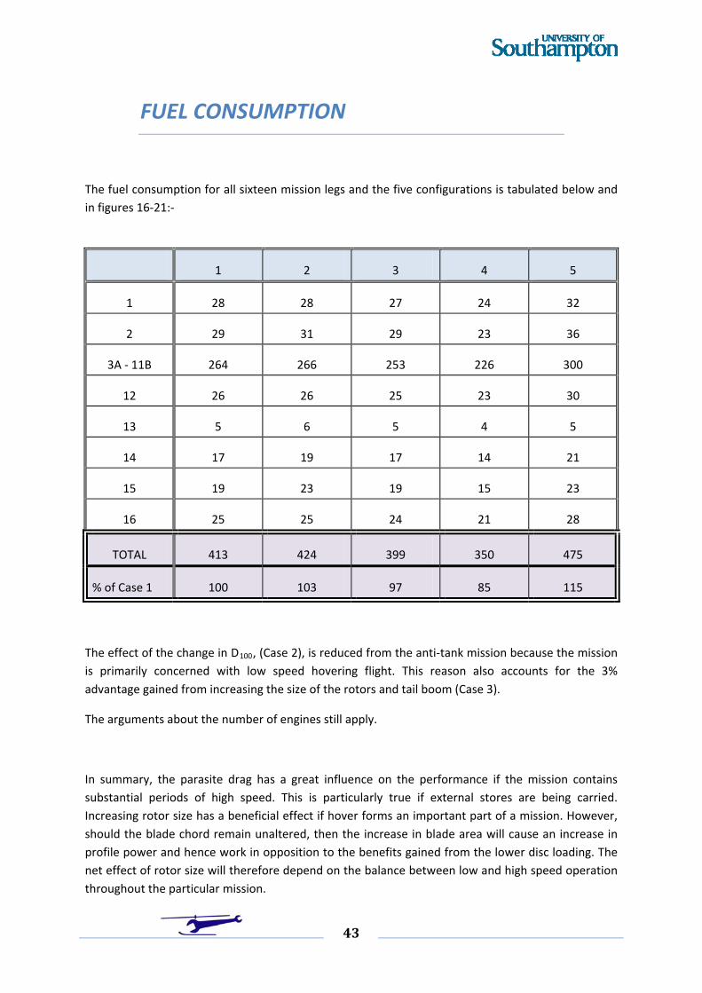
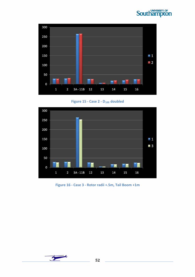
FUEL CONSUMPTION 

 

The fuel consumption for all sixteen mission legs and the five configurations is tabulated below and 

in figures 16‐21:‐ 

 

  1  2  3  4  5 

1  28  28  27  24  32 

2  29  31  29  23  36 

3A ‐ 11B  264  266  253  226  300 

12  26  26  25  23  30 

13  5  6  5  4  5 

14  17  19  17  14  21 

15  19  23  19  15  23 

16  25  25  24  21  28 

TOTAL  413  424  399  350  475 

% of Case 1  100  103  97  85  115 

 

The effect of the change in D100, (Case 2), is reduced from the anti‐tank mission because the mission 

is  primarily  concerned  with  low  speed  hovering  flight.  This  reason  also  accounts  for  the  3% 

advantage gained from increasing the size of the rotors and tail boom (Case 3). 

The arguments about the number of engines still apply. 

 

In  summary,  the  parasite  drag  has  a  great  influence  on  the  performance  if  the mission  contains 

substantial  periods  of  high  speed.  This  is  particularly  true  if  external  stores  are  being  carried. 

Increasing rotor size has a beneficial effect if hover forms an important part of a mission. However, 

should the blade chord remain unaltered, then the  increase  in blade area will cause an  increase  in 

profile power and hence work in opposition to the benefits gained from the lower disc loading. The 

net effect of rotor size will therefore depend on the balance between low and high speed operation 

throughout the particular mission. 

 

 

  

 

44

 

 

 

The effect of the numbe

 

FIGURES 

r of engines on fuel consumption is of major importance. 

s Thrust

Drag

Weight

 

Figure 1 ‐ Force Balance of the Main Rotor 

 

 

  

 

45

 

 

0.8

0.85

0.9

0.95

1

1.05

1.1

0 0.1 0.2 0.3 0.4 0.5

Blockage Factor

 

Figure 2 ‐ Rotor Blockage Variation with Advance Ratio 

0

500

1000

1500

2000

2500

Power (kW)

Forward Speed (m/s)

Main Rotor Power Components

Total

Parasite

Profile

Induced

 

Figure 3 ‐ Variation of Main Rotor Powers Components in Forward Flight 

 

 

  

 

46

 

 

0

200

400

600

800

1000

1200

1400

0 20 40 60 80 1

Power (kW)

Forward Speed (m/s)

00

 

Figure 4 ‐ Total Power Variation in Forward Flight 

0.0

0.2

0.4

0.6

0.8

1.0

0 20 40 60 80 1

Endurance

00

Endurance ‐ Full Endurance ‐ Simple 

Figure 5 – Endurance (hr) Variation in Forward Flight 

 

 

  

 

47

 

 

0

50

100

150

200

0 20 40 60 80

Range

100

Range ‐ Full Range ‐ Simple 

Figure 6 – Range (km) Variation in Forward Flight 

0

50

100

150

200

0 20 40 60 80 10

Range

0

Range ‐ Full Range ‐ Simple

0.0

0.2

0.4

0.6

0.8

1.0

0 20 40 60 80 100

Endurance

Endurance ‐ Full Endurance ‐ Simple

A

A

B

C

 

Figure 7 ‐ Location of Endurance (hr) and Range (km) Maxima 

 

 

 

  

 

48

 

 

 

 

‐600

‐400

‐200

0

200

400

600

800

1000

1200

1400

0 10 20 30 40 50 60 70 80 90 100

P TOTAL Best Range Simple Best Range Full 

Figure 8 ‐ Graphical Construction of Performance Extrema 

 

Anti Tank Mission Fuel Usage (kg) 

 

 

  

 

49

 

 

 

Figure 9 ‐ Case 1 ‐ Basic Aircraft 

 

Figure 10 ‐ Case 2 ‐ D100 doubled 

 

 

  

 

50

 

 

 

Figure 11 ‐ Case 3 ‐ Rotor Radii +.5m, Tail Boom +1m 

 

Figure 12 ‐ Case 4 ‐ No. of Engines = 1 

 

 

  

 

51

 

 

 

Figure 13 ‐ Case 5 ‐ No. of Engines = 3 

 

ASW Mission Fuel Usage (kg) 

 

Figure 14 ‐ Case 1 ‐ Basic 

 

 

  

 

52

 

 

 

Figure 15 ‐ Case 2 ‐ D100 doubled 

 

Figure 16 ‐ Case 3 ‐ Rotor radii +.5m, Tail Boom +1m 

 

 

 

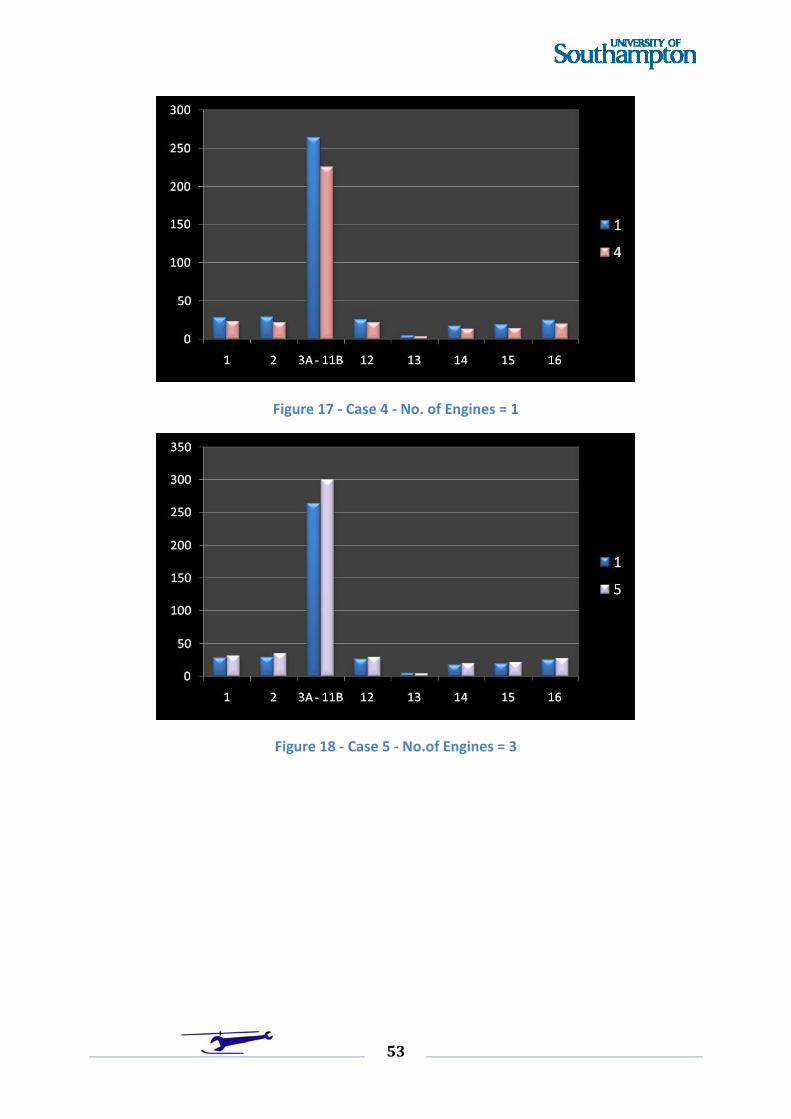
Figure 17 ‐ Case 4 ‐ No. of Engines = 1 

 

Figure 18 ‐ Case 5 ‐ No.of Engines = 3 

 

 

  

 

53