Advection Boundary Condition

8/3/2019 Advection Boundary Condition

http://slidepdf.com/reader/full/advection-boundary-condition 1/25

4-1

4.5. Boundary Conditions for Hyperbolic Equations

(ref. Chapter 8, Durran)

4.5.1. Introduction

In numerical models, we have to deal with two types of boundary conditions:

a) Physical

e.g., ground (terrain), coast lines, the surface of a car when modeling flow around a moving car.

internal boundaries / discontinuities

b) Artificial / Numerical

must impose them to limited integration domain, but they should act as if they don't exist

the boundary should be transparent to "disturbances" moving across the boundary

there can be different kinds of forcing at the boundaries, e.g., lifting by mountain slope and heating at the

surface

these boundaries should be well-posed mathematically

often we have to over-specify the boundary condition, e.g., when a grid is one-way nested inside the coarsergrid

it has been shown that no well-posed lateral b.c. exists for the shallow water equations or for the Navier-

Stokes equations

still a lot of debate in this area. B.C. are often critical because they can exert enormous control over the

interior solution



4-2

As you might suspect, B.C. for hyperbolic problems are closely related to the theory of characteristics –

information propagates along characteristic paths.

Consider the well-posed problem in a 1-D domain 0 x ≥ (only one b.c. at x=0, but to solve the problem numerically,

we have to place a computational boundary somewhere at x>0).

0u u

c

t x

∂ ∂+ =

∂ ∂

(36)

I.C.: u( x,0) = f ( x)

B.C.: u(0,t ) = g( x)

And f (0) = g(0) for consistency between the I.C. and B.C.

From our earlier discussion, we know that

du = 0 along dx / dt = c, i.e., x = ct + β

where β is a constant to be determined by I.C.

Look at an x-t diagram:



4-3

Consider the characteristic passing through (x1 , t1):

u( x1 , t 1) = u( x2, 0) = f ( x2 ) = f ( x1 – ct 1 )

For any ( x, t ) such that x – ct ≥ 0, that solution can be related to the I.C. f ( x), i.e.,

u( x, t ) = f ( x- ct ) for x ≥ ct .

Consider now point ( x3, t 3). In this case, using the MOC, we see that

u( x3, t 3) = u(0, t *) = g( t 3 – x3 / c)

solution has dependency on the B.C. g(t ) and not the I.C. Thus in general,



4-4

u( x, t ) = g(t - x / c) if x < ct .

Now, if we have to impose a boundary condition at x = L, the problem becomes ill-posed because we've over-

specified the solution at x = L, i.e., no condition is required there!

It is unlikely that the solution given by f ( x1-ct 1), for example, will match whatever condition we impose at x= L. The

problem is that, in the general case, the B.C. depends on the solution, which isn't known at x = L a priori! What

happens if we have a whole spectrum of waves that propagate at difference speeds? We can't supply a B.C. foreach one!

4.5.2. Number of Boundary Conditions

For the previous 1-D advection problem, we need only one B.C. Now let's look at the 1-D shallow water equations

in the absence of mean flow:

' '0

u

t x

φ ∂ ∂+ =

∂ ∂(37a)

' '0

u

t x

φ ∂ ∂+ Φ =

∂ ∂(37b)

0 x L≤ ≤ .

Recall the characteristic form of the system for Φ = constant

0 A A

t x

∂ ∂

∂ ∂ + Φ = (38a)



4-5

0 B B

t x

∂ ∂

∂ ∂ − Φ = (38b)

where / and / A u B uφ φ = + Φ = − Φ .

Clearly, there are 2 pure advection equations in the Riemann invariants A and B, with wave speeds of ± Φ . We

have separated the waves, or eigenvalues, and in general, the number of boundary conditions equals to the number

of eigenvalues. This doesn't tell what the B.C. should be, however. Just how many.

In practice, the number of B.C. also depends on the particular grid structure used.

In our case,

1λ = + Φ right moving wave must specify L.H. boundary condition

2λ = − Φ left moving wave must specify R.H. boundary condition

Note that we specify the B.C. from where the wave originates, but not to where it's going!

4.5.3. Sample B.C. and Wave Reflection

For limited area models that contain artificial lateral boundaries, we desire to let incident waves pass through

without reflection, i.e., as if the boundary wasn’t there at all. This is the behavior for the exact or differential

solution.



4-6

t = t1 t = t2

Consider 1-D linear advection:

0u u

ct x

∂ ∂+ =

∂ ∂c >0 and constant, x−∞ ≤ ≤ ∞ , 0t ≥ . (39)

To look at reflection at the boundary, we need consider only the spatial derivative.

20

x

uc u

t δ

∂+ =

∂ x L−∞ ≤ ≤ (40)

This equation describes a right-moving wave. If there is reflection at x=L, the reflected wave must be

computational in origin, because the physical equation doesn't support left-moving wave.

Our center-in-space discretization connot be applied at x=L (since it needs u at L+1), so something else must be

done. Note that no B.C. should be speficied at x=L, except due to the fact that computer has limited memory and

computing power so you can't make the computational domain infinitely large.



4-7

Approximations to the PDE at x=L:

1. u L = 0 Fixed or rigid boundary

2. u L = u L-1 Zero gradient (about u L-∆ x /2)

3. u L = 2u L-1 - u L-2 Linear extrapolation

One can also use special forms of the PDE, e.g., upstream at the boundary:

1

n n

L L

L

u u uc

t x

−∂ −= −

∂ ∆upstream

1 23 4 4

2

n n n

L L L

L

u u u uc

t x

− −∂ − += −

∂ ∆second-order upstream

Question: What happens to a wave when these B.C. are applied to the semi-discrete (semi because time remains inderivative form therefore there is no time discretization error – we focus on error caused by spatial discretization)

equation (40)?

Assume solutions of the form

exp[ ( )] ju A i kx t ω = − , Plug it into Eq.(40), we get

( ) ( )0

2

j j

ik x ik xi kx t i kx t e e

i Ae cAe x

ω ω ω

∆ − ∆− − −

− + =∆

sin( ) sin( )( )d

d d

c k x c p p k x

x x

ω ∆

= = = ∆

∆ ∆



4-8

Now, for the PDE we have

ee

k x p ckc c

x xω

∆= = =

∆ ∆

where pe = exact value of k ∆ x. We now want to compare these two frequencies.

Note that, in the F.D. solution, two values of k ∆ x correspond to a single ωd, whereas in the exact solution, ω e is

linear in k ∆ x.



4-9

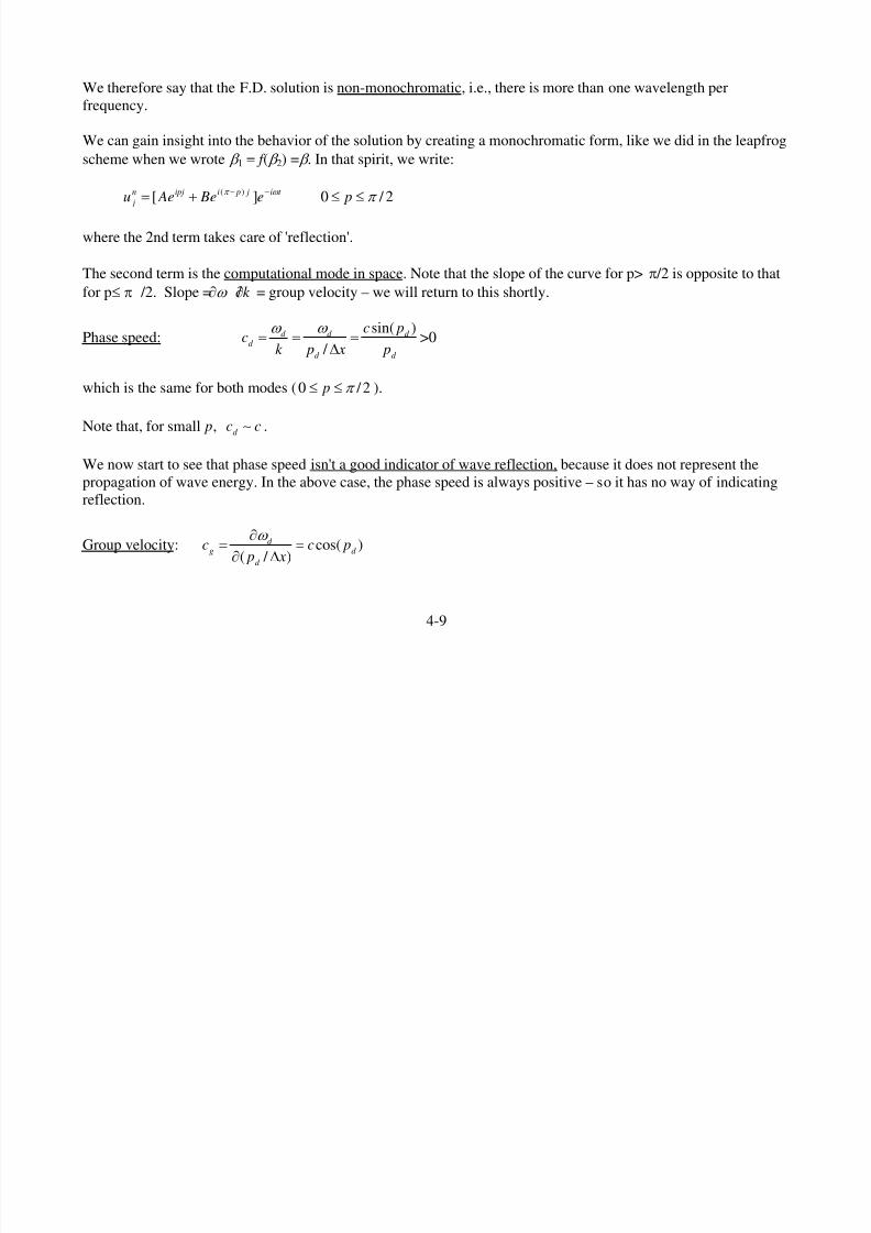
We therefore say that the F.D. solution is non-monochromatic, i.e., there is more than one wavelength per

frequency.

We can gain insight into the behavior of the solution by creating a monochromatic form, like we did in the leapfrog

scheme when we wrote β 1 = f ( β 2) = β . In that spirit, we write:

( )[ ] 0 / 2n ipj i p j i t

ju Ae Be e pπ ω π − −= + ≤ ≤

where the 2nd term takes care of 'reflection'.

The second term is the computational mode in space. Note that the slope of the curve for p> π /2 is opposite to that

for p≤ π /2. Slope = / k ω ∂ ∂ = group velocity – we will return to this shortly.

Phase speed:sin( )

/

d d d d

d d

c pc

k p x p

ω ω = = =

∆

>0

which is the same for both modes (0 /2 p π ≤ ≤ ).

Note that, for small p, d c c∼ .

We now start to see that phase speed isn't a good indicator of wave reflection, because it does not represent thepropagation of wave energy. In the above case, the phase speed is always positive – so it has no way of indicating

reflection.

Group velocity: cos( )( / )

d g d

d

c c p p x

ω ∂= =

∂ ∆



4-10

cg > 0 for pd = p (0 / 2 p π ≤ ≤ )

cg< 0 for pd = π - p.

If cg < 0, this means that energy is propagating in a direction opposite to the cg of the exact solution (which is

positive), such negatively propagating waves may be a result of reflection at the boundary (it can also be because

of other reasons).

We can interpret reflection in terms of group velocity - the reflected waves (or more accurately wave packets)transport energy in the opposite direction upon reflection.

It is possible to determine the amplitude, r , of the reflected wave. See Matsuno, JMSJ, 44, 145-157 (1966).

Let A = amplitude of incident wave = 1.0

B(=r ) = amplitude of reflected (computational mode) wave

(notation is from the monochromatic solution)

( )i t ipj i p j

ju e e re

ω π − −⎡ ⎤= +⎣ ⎦

Example: Zero gradient lateral boundary condition

u L = u L-1

without loss of generality, we can let L=0

u0 = u-1



4-11

With j=0 and j= -1 in our solution, we have

( )1

ip i pr e re

π − − −+ = +

where 'd' on p has been dropped, and the i t e

ω − 'cancels' via linear independence for a single frequency ω.

(1 ) 1ip ipr e e

−+ = −

/ 2 / 2 / 2

/ 2 / 2 / 2

1 ( ) sin( / 2)

1 ( ) cos( / 2)

ip ip ip ipip

ip ip ip ip

e e e e i pr e

e e e e p

− − − −−

− − −= = =+ +

=-[cos( ) sin( )] tan( / 2) p i p i p−

| r | = tan ( p /2) where p = k ∆ x = pd (0 / 2 p π ≤ ≤ )

Note: The reflected amplitude depends upon both k of the incident wave and ∆ x.

4∆ x wave ( p = π /4 ) | r | = 1.0 complete reflection without change in amplitude.

32 ∆ x wave ( p=π /16) | r | = 0.0982 relatively weak reflection

| r | ~ 1/ (incident wavelength).

Short waves are reflected much more than long waves – it is understandable – infinitely long waves, i.e., constant

field, should pass through a zero gradient boundary freely.



4-12

4.5.4. Refelction for the Shallow Water Eqautions – Radiation BoundaryCondition

Let's consider a semi-discrete shallow water equations system:

2 2

2 2

ˆ 0

ˆˆ

0

x x

x x

uu u

t

u ut

δ δ φ

φ

δ φ δ

∂+ + Φ =

∂

∂

+ + Φ =∂

Here, we let ˆ / φ φ = Φ so that the two equations are completely symmetric. This is to make our discussion easier.

The system describes waves moving in the + or – directions depending upon the relationship of u and Φ1/2. If u <

0 and | u | > Φ1/2, then the wave will go to the left.

Often we want to allow such waves to pass through an artificial lateral boundary while minimizing the reflection.

Because we have 2 waves in this system, there will be 2 physical modes and 2 computational modes – one for each

wave. Using the same analysis as before, we have

Physical Modes:

1 1( )

1 1 1 1ˆ( , ) ( , ) with sin( )i k x t u

u u e k x x

ω φ φ ω

− + Φ= = ∆

∆

2 2( )

2 2 2 2ˆ( , ) ( , ) with sin( )

i k x t uu u e k x

x

ω φ φ ω − − Φ= = ∆

∆



4-13

where andu φ are the amplitude of u andφ̂ , respectively.

Computational Modes (the "image" about p=π /2)

3 3( )

3 3 3 3 3 1( , ) ( , ) with sin( ) andi k x t u

u u e k x k k x x

ω π φ φ ω

− + Φ= = ∆ = −

∆ ∆

4 4( )

4 4 4 4 4 2( , ) ( , ) with sin( ) andi k x t u

u u e k x k k x x

ω π φ φ ω

− − Φ= = ∆ = −∆ ∆

Note: ω3 = ω1 and ω4 = ω2, i.e., 2 horizontal wavenumbers corresponding to the same value of frequency.

Let's now look at the directions of phase speed and group velocity of these modes.

Phase Speed

Physical modes: cp > 0 for both modes if u > Φ1/2

cp > 0 for one and < 0 for the other if 0<u <Φ1/2

Computational Modes: Same as above

Group Velocity

cg1 = - cg3 = (u + Φ1/2) cos( k 1 ∆x)

cg2 = - cg4 = (u - Φ1/2) cos( k 2 ∆x)

where 0 ≤ k 1,2∆x ≤ π /2 for a monochromatic solution. Thus there are always 2 group velocities > 0 and two < 0.



4-14

Example: Consider what happens at an outflow boundary when Φ1/2> u > 0. Here, we want to specify a boundary

condition at x = L.

Now, we know that

u = u1 + u2 + u3 + u4

φ̂ = φ̂ 1 + φ̂ 2 + φ̂ 3 + φ̂ 4

From the analytical solution, we know that

ω = k (u +Φ1/2)

cp = cg,

i.e., the energy and phase always propagate in the same direction.

Going back to our 4 solutions, we find that for Φ1/2> u > 0 (this case only),

Mode 1: Phase > 0, group > 0 physical mode

Mode 2: Phase < 0 group < 0 physical mode

Mode 3: Phase > 0 group < 0 computational mode

Mode 4: Phase < 0, group > 0

computational mode

Now, mode 1 is the physical incident wave, and if it gets reflected, its energy will come back in modes 2 and 3

because their group velocities are negative. The reflection won’t show up as mode 4.

As a result, we can analyze the reflection in terms of 1, 2 and 3 only:



4-15

31 1 2 2( ) Rik xik x i t ik x i t

u e re e e eω ω − −= + +

31 1 2 2ˆ( ) R

ik xik x i t ik x i t

e re e e e

ω ω

φ

− −

= + − (41)

Why the minus sign on the last term in the φ equation?

Recall that the Riemann invariant of the right-moving wave is u1,3 + φ1,3 / Φ1/2

= u1,3 + φ̂ 1,3

31 1

1,3 1,3ˆ 2( )

ik xik x i t u e re e

ω φ

−+ = + ,

which is the physical mode 1 with its computational counterpart 3. The minus sign is needed to make sure that theabove 2 equations when added together form a Riemann invariant that does not involve left-ward propagation

waves - those that are supported by the other characteristic equation, i.e, ˆ ˆ( ) / ( ) ( ) / 0u t u u xφ φ ∂ − ∂ + − Φ ∂ − ∂ = .

Now, let's examine the reflection properties for various boundary conditions applied to this particular semi-discrete

form of the shallow water equations.

First, it's important to recognize that the solutions at the boundary must be continuous frequency of the incident

and reflected waves must be identical at the boundary. So, if ω1 = ω2 (ω1 = ω3 already), we have,

2 1

uk k

u

1/2

1/2

+ Φ≈

− Φ.

incident

physical

mode

reflected

computational

mode

(amplitude=r)

reflected

physical

mode



4-16

[Here we assumed that k ∆ x is small (good for high resolution) so thatsin( )k x k x∆ ≈ ∆ ].

Therefore, k 2 > k 1, or the reflected wave is always smaller in scale than the incident wave. (Note that at a critical

layer where Φ1/2=u , the analysis is not valid and a different approach has to be taken.)

Now, let's apply the above analysis to different types of boundary conditions.

Based on earlier analysis, we rewrite (41) as

11 2

1 1 2

( )

[ R ] ( )

[ ( 1) R ] ( )

i k xik x ik x i t x

ik x ik x ik x j i t

u e re e e

e r e e e x j x

π

ω

ω

ω ω ω ω − −∆

1 2 3

−

= + + = = =

= + − + = ∆

Similarly we have

1 1 2[ ( 1) R ]ik x ik x ik x j i t e r e e e

ω φ −= + − −

Case I: u L = 0, i.e., we have the rigid wall.

uL = 0 0 (if u=0, i.e., can't have u 0if u=0 at the boundary) L x

φ ∂= ≠

∂

Let L =0 without loss of generality:



4-17

therefore u0 = 0, φ0 = φ-1 .

For the first equation, we have

1 + r + R = 0

For the second, we have

1 1 21 [ R ]ik x ik x ik x

r R e re e− ∆ − ∆ − ∆+ − = − −

Assuming that 1 xe x≈ + , we have

1 1 21 1r R ik x r rik x R Rik x+ − = − ∆ − + ∆ − + ∆

1 1 2( ) / 2r i x k rk Rk = ∆ − + +

Equating the real and imaginary parts, we have

r = 0

R = -1

0-1



4-18

k 1 = - k 2.

We showed earlier that

2 1

uk k

u

1/2

1/2

+ Φ=

− Φ

which agrees with current result when u =0.

In summary, we found total reflection in the physical mode, which is the expected condition for a rigid lateral

boundary. This is also undesirable if the true problem does not actually have a boundary here. When there is indeed

a wall, we often use the so-called mirror boundary condition (as in ARPS for B.C. option one), which finds it basis

in our analysis.

Case II: Wave radiating lateral boundary condition

At the boundary L, we use

* 1( ) 0 L Lu u u

u ct x

−∂ −+ + =

∂ ∆

to replace the momentum equation. For φ, use the governing equation itself with one-sided difference:

1 1 L L L Lu uu

t x x

φ φ φ − −∂ − −+ + Φ

∂ ∆ ∆= 0.



4-19

In the above, c*

is an estimate of the dominant wave speed at the lateral boundary (can be set constant, or computed

as was done by Orlanski 1976).

Doing a reflection analysis, we find (show for yourselves) that

*

*

( )( )(for reflected physical mode)

( )( )

u c R

u c

1/2 1/2

1/2 1/2

− Φ Φ −=

+ Φ Φ +

r = 0 (for computational mode)

[See Klemp and Lilly, 1978, JAS, p78]

If we do a good job of estimating c*, then we can make R~0.

Again, the reflection is in the physical mode, and that is not good. Keep in mind that this analysis assumes that

k ∆x 1.

In complicated models, one typically replaces the normal momentum equation at the lateral boundary with

*( ) 0u u

u ct x

∂ ∂+ + =

∂ ∂(42)

It neglects pressure gradient force responsible for the wave propagation, the effect can be thought as beingaccounted for in c

*).

In (42), the sign of u + c*

determines inflow or outflow boundary. Other equations are then solved using their

original governing equations, with one-sided difference when necessary. This type of condition is called

Sommerfeld radiation condition. Orlanski (1976) applies equation like (42) to all variables, but in practice, it does

not work very well – it leads to over-specification of conditions and enhancement of the computational mode.



4-20

ARPS has options for four variations for radiation lateral boundary conditions – all follow Sommerfeld condition,

the difference being the way c* is determined and whether (42) is applied in large or small time steps.

Klemp and Lilly (1978) gives more details on the analysis of radiation lateral boundary conditions.

It should be noted that, in terms of characteristics, our shallow water system is

1/ 2( ) 0 A A

ut x

∂ ∂+ + Φ =∂ ∂

1/ 2( ) 0 B B

ut x

∂ ∂+ − Φ =

∂ ∂

with A = u + φ / Φ 1/2

and B = u - φ / Φ 1/2

, the Riemann invariants.

The radiation condition *( ) 0u u

u ct x

∂ ∂+ + =

∂ ∂is equivalent to setting to zero the amplitude of B. So, the radiation

B.C. can be regarded as a condition written in terms of the characteristics, and that's why a PGF does not occur. In

fact, if B=0, at the lateral boundary, then

A + B = A + 0 = 2u

∴ 1/ 2(2 ) (2 )( ) 0

u uu

t x

∂ ∂+ + Φ =

∂ ∂

which is the Radiation Condition we used.



4-21

References:

Orlanski, I., 1976: A simple boundary condition for unbounded hyperbolic flows. J. Comput. Phys., 21, 251-269.

Klemp, J. B., and D. K. Lilly, 1978: Numerical simulation of hydrostatic mountain waves. J. Atmos. Sci., 35, 78-

107.

4.5.4. Other Boundary Conditions

Rayleigh Damping (Sponge)

Here we include a regional (zone) next to the lateral boundary in which zero-order (Rayleigh) damping is applied

to the prognostic variables, to 'absorb' incident wave energy and damp possibly reflected energy.

1 1

2 ( )( ) ( ) / ( )n n

t u r x u u u u xδ τ − −= − − = − −



4-22

where r is the Rayleigh damping coefficient and τ the corresponding e-folding time of damping. The smaller r is,

the longer it takes to damp.

Rayleigh damping is usually needed when the lateral boundary conditions are over-specified, such as the case of

externally forced boundary (e.g., when a grid is forced by the solution of another model, the coarse grid solution of

the same model or by analysis – the case of one-way nesting). ARPS uses Rayleigh damping with externally forced

boundary option.

Viscous sponge

It takes the form of second-order diffusion

1

2

n

t xxu K uδ δ −=

In this case, short waves are selectively damped. It does not damp long reflected waves effectively, however. It isoften used in combination with the Rayleigh damping, as in the ARPS.

Top boundary condition

In atmospheric models, the top boundary of the computational domain often has to be placed at a finite height –

creating an artificial top boundary. Vertically propagating, e.g., internal gravity, waves can reflect off the boundary

and interact with flow below – creating problems. One example of radiation top boundary condition is that of

Klemp and Durran (1983). See also Durran section (8.3.2).

Reference:

Klemp, J. B., and D. R. Durran, 1983: An upper boundary condition permitting internal gravity wave radiation in

numerical mesoscale models. Mon. Wea. Rev., 111, 430-444.



4-25

Pearson, R. A., 1974: Consistent boundary conditions for numerical models of systems that admit dispersive waves. Journal of theAtmospheric Sciences, 31, 1481--1489.

Pearson, R. A., and J. L. McGregor, 1976: An open boundary condition for models of thermals. Journal of the Atmospheric Sciences,

33, 447-455.*Perkey, D. J., and C. W. Kreitzberg, 1976: A time-dependent lateral boundary scheme for limited-area primitive equation models.

Monthly Weather Review, 104, 744-755.

Raymond, W. H., and H. L. Kuo, 1984: A radiation boundary condition for multi-dimensional flows. Quarterly Journal of the RoyalMeteorological Society, 110, 535-551.

Rudy, D. H., and J. C. Strikwerda, 1980: A nonreflecting outflow boundary condition for subsonic Navier-Stokes calculations. Journal

of Computational Physics, 36, 55-70.

Sloan, D. M., 1983: Boundary conditions for a forth order hyperbolic difference scheme. Mathematics of Computation, 41, 1-11.Sundstrom, A., 1977: Boundary conditions for limited-area integration of the viscous forecast equations. Beitrage zur Physik det

Atmosphare, 50, 218-224.

Sundstrom, A., and T. Elvius, 1979: Computational problems related to limited-area modeling. Numerical Methods in AtmosphericModels, Volume II, GARP Publications Series, No. 17.

Tadmor, Eitan, 1983: The unconditional instability of inflow-dependent boundary conditions in difference approximations to

hyperbolic systems. Mathematics of Computation, 41, 309-319.

Advection Boundary Condition

Documents

Transcript of Advection Boundary Condition