Journal of Computational Physics 229 (2010) 8733–8749

Contents lists available at ScienceDirect

Journal of Computational Physics

journal homepage: www.elsevier .com/locate / jcp

Absorbing boundary conditions for the Euler and Navier–Stokesequations with the spectral difference method

Ying Zhou *, Z.J. WangDepartment of Aerospace Engineering, Iowa State University, 2271 Howe Hall, Ames, IA 50010, United States

a r t i c l e i n f o

Article history:Received 7 April 2010Received in revised form 16 July 2010Accepted 10 August 2010Available online 21 August 2010

Keywords:High-order methodsNavier–Stokes equationsUnstructured gridsSpectral differenceDiscontinuous GalerkinNon-reflecting boundary conditionAbsorbing sponge zonePerfectly matched layer

0021-9991/$ - see front matter � 2010 Elsevier Incdoi:10.1016/j.jcp.2010.08.007

* Corresponding author. Tel.: +1 515 295 5539.E-mail address: ying@iastate.edu (Y. Zhou).

a b s t r a c t

Two absorbing boundary conditions, the absorbing sponge zone and the perfectly matchedlayer, are developed and implemented for the spectral difference method discretizing theEuler and Navier–Stokes equations on unstructured grids. The performance of both bound-ary conditions is evaluated and compared with the characteristic boundary condition for avariety of benchmark problems including vortex and acoustic wave propagations. Theapplications of the perfectly matched layer technique in the numerical simulations ofunsteady problems with complex geometries are also presented to demonstrate itscapability.

� 2010 Elsevier Inc. All rights reserved.

1. Introduction

In the last two decades, there have been intensive research efforts on high-order methods for unstructured grids. Suchmethods provide unprecedented geometric flexibility and accuracy for real world applications. An incomplete list of notableexamples includes the spectral element method [51], multi-domain spectral method [43,44], k-exact finite volume method[6], WENO methods [27], discontinuous Galerkin (DG) method [7,12,13], high-order residual distribution methods [1], spec-tral volume (SV) [49,56,64–66] and spectral difference (SD) methods [40,47,50,57,58,67,68]. Spectral difference method orig-inated in the staggered grid multi-domain spectral method [43,44]. Thereafter it was generalized to simplex elements by Liuet al. [47,48]. More recently, a weak instability was discovered by Van Den Abeele et al. [63] and Huynh [41]. The use ofGauss quadrature points and the two ending points as the flux points fixes the problem, and it was proved to be stableby Jameson [42]. A high-order SD method for three-dimensional Navier–Stokes equations on unstructured hexahedral gridsdeveloped by Sun et al. [57,58] is used in this paper.

For the numerical simulations of fluid dynamic and aeroacoustic problems, a proper artificial computational boundarycondition is needed to minimize the reflection of out-going waves, which can contaminate the physical flow field. Thisboundary condition is usually called the non-reflecting boundary condition or absorbing boundary condition. It remains acritical component and a difficult challenge in the development of computational fluid dynamics (CFD) and computationalaeroacoustics (CAA) algorithms. Significant progresses have been made in this research as reviewed extensively by Colonius[16] and Hu [34].

. All rights reserved.

8734 Y. Zhou, Z.J. Wang / Journal of Computational Physics 229 (2010) 8733–8749

The non-reflecting boundary condition based on the characteristics of the Euler equations was developed as one of thefirst attempts to minimize the reflection of out-going waves, e.g., in [21,54,61]. In the Godunov-type finite volume methods,the characteristic boundary condition (CBC) based on the linearized one-dimensional Euler equations [45,69,26] is wide-spread and works well in the numerical simulations of steady problems. For multi-dimensional problems, the performanceof the CBC degrades if the wave propagation direction is not aligned with the boundary face normal direction. More efficientand accurate non-reflecting boundary conditions are needed to handle problems like vortex dominated flows and wavepropagation problems.

The absorbing boundary condition (ABC) also receives much attention from the electromagnetic and acoustic communi-ties. Engquist and Majda [18] made a pioneering contribution to in this area. Their boundary conditions were constructed tominimize reflections of waves traveling in directions close to perpendicular to the boundary. Higdon [25] further developedthe boundary conditions in a simpler and more general form. Another well-known ABC firstly proposed by Bayliss and Turkel[8,9] was developed in an asymptotic expansion of the solution in the far field and annihilate of the leading terms. This typeof ABC is widely used in scattering problems to absorb the outgoing disturbances. In the present study, we consider flowproblems with strong nonlinear viscous wakes. As a result, we did not pursue the above boundary conditions.

An innovative class of approaches of non-reflecting/absorbing boundary conditions uses extra artificial zones to reducewave reflections. They are the loosely termed ‘‘zonal techniques” [34]. In this type of technique, additional zones surround-ing the physical domain are introduced so that in the added zones either the outgoing disturbances/waves are attenuatedand thus the reflections are minimized, or the mean flow is altered gradually to be supersonic and thus all disturbances/waves are out-going. Two popular zonal techniques are the absorbing sponge zone (ASZ) technique [19] and perfectlymatched layer (PML) technique [39].

The ASZ technique used in this paper was first proposed for the direct acoustic simulation by Colonius et al. [15] and laterin a different approach by Ta’asan et al. [59]. It was further developed and theoretically analyzed by Freund [19] and Bodony[11]. Inside the ASZ domain, one source term�rðQ � QÞ is added to the right-hand-side of the governing equations such thatthe solution Q is gradually tuned to the proposed solution Q . In order to diminish the reflected error generated at the phys-ical/ASZ interface, the absorbing coefficient r increases smoothly from zero at the interface to a positive value at the end ofthe ASZ domain. This technique is widely used in the CAA community for its simplicity and effective performance.

The PML technique was originally developed as an absorbing boundary condition for computational electromagnetic [10]in which the Maxwell equations are numerically solved, and quickly became the method of choice in the computational elec-tromagnetic community [20,53]. The PML equations are formulated such that the amplitude of the out-going waves enteringthe PML domain can be exponentially reduced while causing as little numerical reflection as possible. It was also found to bea good choice for computational aeroacoustics and computational fluid dynamics [14,22–24,62]. The PML technique wasfirstly extended to the linearized Euler equations in [28]. However the direct adaption of the split formulation to the Eulerequations was found to be unstable in the PML domain [28,29,2–5,60,70]. Hu [30–33,35,52] found that for the PML techniqueto yield stable absorbing boundary condition, the phase and group velocities of the physical wave supported by the govern-ing equations must be consistent and in the same direction, and a stable formulation of a PML for the linearized Euler equa-tions was proposed. It was proved in [36] that theoretically no reflection will be generated in the PML domain for linearizedEuler equations. Further extension of the PML technique to nonlinear Euler and Navier–Stokes equations was given in[37,39]. For nonlinear equations, though the conversion of the equations is not perfectly matched to the original equationsdue to the nonlinearity of flux vectors, the results of the numerical examples show that the proposed absorbing equations arestill effective [37–39].

In this paper, both the ASZ and the PML techniques are extended and implemented for the SD method on hexahedralmeshes. The performance and effectiveness are compared with the CBC based on one-dimensional Euler equations. Thena two cylinder case is employed to test the performance of three boundary conditions with complex geometries and vortexdominant flow.

The rest of the paper is organized as follows. In the next section, the formulation of the spectral difference method isbriefly reviewed. In Sections 3 and 4, the ASZ and PML approaches used in the spectral difference method are presented withthe unstructured hexahedral mesh. In Section 5, numerical tests are presented and discussed. Concluding remarks are givenin Section 6.

2. Review of the multi-domain spectral difference method

2.1. Governing equations

Consider the three-dimensional compressible non-linear Navier–Stokes equations written in the conservation form as

@Q@tþ @F@xþ @G@yþ @H@z¼ 0 ð2:1aÞ

on domain X� ½0; T� and X � R3 with the initial condition

Qðx; y; z;0Þ ¼ Q 0ðx; y; zÞ ð2:1bÞ

Y. Zhou, Z.J. Wang / Journal of Computational Physics 229 (2010) 8733–8749 8735

and appropriate boundary conditions on @X. In (2.1), x; y, and z are the Cartesian coordinates and ðx; y; zÞ 2 X; t 2 ½0; T� de-notes time. Q is the vector of conserved variables, and F; G and H are the fluxes in the x; y and z directions, respectively,which take the following form

Q ¼

qqu

qvqw

E

8>>>>>><>>>>>>:

9>>>>>>=>>>>>>;ð2:1cÞ

F ¼ Fi � Fm ¼

qu

qu2 þ p

qumquw

ðEþ pÞu

8>>>>>><>>>>>>:

9>>>>>>=>>>>>>;�

0sxx

sxy

sxz

usxx þ msxy þwsxz � qx

8>>>>>><>>>>>>:

9>>>>>>=>>>>>>;ð2:1dÞ

G ¼ Gi � Gm ¼

qmqum

qm2 þ p

qmw

ðEþ pÞm

8>>>>>><>>>>>>:

9>>>>>>=>>>>>>;�

0sxy

syy

syz

usxy þ msyy þwsyz � qy

8>>>>>><>>>>>>:

9>>>>>>=>>>>>>;ð2:1eÞ

H ¼ Hi � Hm ¼

qw

quw

qmwqw2 þ p

ðEþ pÞw

8>>>>>><>>>>>>:

9>>>>>>=>>>>>>;�

0sxz

syz

szz

usxz þ msyz þwszz � qz

8>>>>>><>>>>>>:

9>>>>>>=>>>>>>;ð2:1fÞ

with the total energy written as

E ¼ pc� 1

þ 12qðu2 þ m2 þw2Þ

viscous stress terms written as

sxx ¼ 2l @u@x� 2

3l @u

@xþ @m@yþ @w@z

� �syy ¼ 2l @m

@y� 2

3l @u

@xþ @m@yþ @w@z

� �szz ¼ 2l @w

@z� 2

3l @u

@xþ @m@yþ @w@z

� �sxy ¼ l @u

@yþ @m@x

� �; sxz ¼ l @u

@zþ @w@x

� �; syz ¼ l @w

@yþ @m@z

� �

and heat transfer terms

qx ¼ �k@T@x; qy ¼ �k

@T@y

; qz ¼ �k@T@z

where fq;u;v ;w; pg are the primitive variables of density, velocities and pressure, l is coefficient of viscosity and k is thecoefficient of thermal.

2.2. Coordinate transformation

In the SD method, it is assumed that the computational domain is divided into non-overlapping unstructured hexahedralcells or elements. In order to handle curved boundaries, both linear and quadratic isoparametric elements are employed,with linear elements used in the interior domain and quadratic elements used near high-order curved boundaries. In orderto achieve an efficient implementation, all physical elements ðx; y; zÞ are transformed into standard cubic elementðn;g; 1Þ 2 ½�1�;1� � ½�1�;1� � ½�1;1� as shown in Fig. 1.

The transformation can be written as

Fig. 1. Transformation from a physical element to a standard element.

8736 Y. Zhou, Z.J. Wang / Journal of Computational Physics 229 (2010) 8733–8749

x

y

z

264375 ¼XK

i¼1

Miðn;g; 1Þxi

yi

zi

264375 ð2:2Þ

where K is the number of points used to define the physical element, ðxi; yi; ziÞ are the Cartesian coordinates of these points,and Miðn;g; 1Þ are the shape functions. For the transformation given in (2.2), the Jacobian matrix J takes the following form

J ¼ @ðx; y; zÞ@ðn;g; 1Þ ¼

xn xg x1

yn yg y1

zn zg z1

264375

The governing equations in the physical domain are then transformed into the standard element, and the transformed equa-tions take the following form

@ eQ@tþ @

eF@nþ @

eG@gþ @

eH@1¼ 0 ð2:3Þ

where

eQ ¼ jJj � QeFeGeH264

375 ¼ jJj nx ny nz

gx gy gz

1x 1y 1z

264375 � F

G

H

264375

2.3. Spatial discretization

In the standard element, two sets of points are defined, namely the solution points and the flux points, illustrated in Fig. 2for a 2D element. The solution unknowns (conserved variables Q) or degrees-of-freedoms (DOFs) are stored at the solutionpoints, while fluxes are computed at the flux points. The solution points in 1D are chosen to be the Chebyshev–Gauss pointsdefined by

Xs ¼ � cos2s� 1

2N� p

� �; s ¼ 1;2; . . . ;N ð2:4Þ

Fig. 2. Distribution of solution points (circles) and flux points (squares) in a standard element for a 3rd-order SD scheme.

Y. Zhou, Z.J. Wang / Journal of Computational Physics 229 (2010) 8733–8749 8737

With solutions at N points, we can construct a degree ðN � 1Þ polynomial in each coordinate direction using the followingLagrange basis defined as

hiðXÞ ¼YN

s¼1;s–i

¼ X � Xs

Xi � Xs

� �ð2:5Þ

The reconstructed solution for the conserved variables in the standard element is just the tensor products of the three one-dimensional polynomials, i.e.,

Qðn;g; 1Þ ¼XN

k¼1

XN

j¼1

XN

i¼1

eQ i;j;k

jJi;j;kjhiðnÞ � hjðgÞ � hkð1Þ ð2:6Þ

The flux points in 1D are chosen to be the ðN � 1Þ Legendre–Gauss quadrature points plus the two end points,�1 and 1. Withfluxes at ðN þ 1Þ points, a degree N polynomial can be constructed in each coordinate direction using the following Lagrangebases defined as

liþ1=2ðXÞ ¼YN

s¼0;s–i

X � Xsþ1=2

Xiþ1=2 � Xsþ1=2

� �ð2:7Þ

Similarly, the reconstructed flux polynomials take the following form:

eF ðn;g; 1Þ ¼XN

k¼1

XN

j¼1

XN

i¼0

eF iþ1=2;j;kliþ1=2ðnÞ � hjðgÞ � hkð1Þ ð2:8aÞ

eGðn;g; 1Þ ¼XN

k¼1

XN

j¼0

XN

i¼1

eGi;jþ1=2;khiðnÞ � ljþ1=2ðgÞ � hkð1Þ ð2:8bÞ

eHðn;g; 1Þ ¼XN

k¼0

XN

j¼1

XN

i¼1

eHi;j;kþ1=2hiðnÞ � hjðgÞ � lkþ1=2ð1Þ ð2:8cÞ

Because the SD method is based on the differential form of the governing equations, the implementation is straightforwardeven for high-order curved boundaries. All the operations are basically one-dimensional in each coordinate direction andeach coordinate direction shares the collocated solution points with others, resulting in improved efficiency. In summary,the algorithm to compute the inviscid flux and viscous flux and update the unknowns (DOFs) consists of the following steps:

1. Given the conserved variables fQ i;j;kg at the solution points, compute the conserved variables fQ iþ1=2;j;kg at the flux pointsusing polynomial (2.6).

2. Note that inviscid flux is a function of the conserved solution and the viscous flux is a function of both the conserved solu-tion and its gradient, taking flux eF for example:

eF ¼ eF i � eFveF i

iþ1=2;j;k ¼ eF iðQ iþ1=2;j;kÞeF viþ1=2;j;k ¼ eF vðQ iþ1=2;j;k;rQ iþ1=2;j;kÞ

8>><>>: ð2:9Þ

Compute the inviscid fluxes eF iiþ1=2;j;k

n oat the interior flux points using the solution fQiþ1=2;j;kg computed at Step 1. Com-

pute the viscous fluxes eF viþ1=2;j;k

n ousing the solution fQiþ1=2;j;kg computed at Step 1 and the gradient of the solutions

frQiþ1=2;j;kg computed based on fQ iþ1=2;j;kg.3. Compute the common inviscid flux at element interfaces using a Riemann solver (2.11), such as the Roe solver [55] and

Russanov solver [57].

eF i ¼ eF iðQL;Q RÞ ð2:11Þ

where Q L and QR represent the solutions from the two elements beside the interface.Compute the common viscous flux at element interfaces using a viscous approach (2.12), such as the averaged approachand DG-like approach [57].eF m ¼ eF mðQ L;QR;rQL;rQ RÞ ð2:12Þ

Then compute the derivatives of the fluxes at all the solution points by using (2.13).

8738 Y. Zhou, Z.J. Wang / Journal of Computational Physics 229 (2010) 8733–8749

@eF@n

!i;j;k

¼XN

r¼0

eF rþ1=2;j;kl0rþ1=2ðniÞ ð2:13aÞ

@eG@g

!i;j;k

¼XN

r¼0

eGi;rþ1=2;kl0rþ1=2ðgjÞ ð2:13bÞ

@ eH@1

!i;j;k

¼XN

r¼0

eHi;j;rþ1=2l0rþ1=2ð1kÞ ð2:13cÞ

4. Update the DOFs using a multistage TVD scheme for time integration of (2.14).

@ eQ i;j;k

@t¼ � @eF

@nþ @

eG@gþ @

eH@1

!i;j;k

ð2:14Þ

For more details about SD method on hexahedral mesh, the readers can refer to [57].

3. Formulation of the absorbing sponge zone (ASZ)

The ASZ technique is a widely used absorbing boundary condition in the computational aeroacoustic community. In gen-eralized coordinates, the conservative form of the Navier–Stokes equations with additional source terms in ASZ domain canbe expressed as

@ eQ@tþ @

eF@nþ @

eG@gþ @

eH@1¼ �eS ð3:1Þ

where

eS ¼ jJj � SS ¼ rðQ � QÞ ¼ r

q� qqu� qu

qm� qmqw� qw

E� E

8>>>>>><>>>>>>:

9>>>>>>=>>>>>>;

and r is the absorbing coefficient.

Basically, there are two choices for the proposed solution Q in ASZ domain. One is to choose Q to be the far field values,and the CBC is usually used at the boundary of the ASZ domain. In this paper, all the numerical cases with ASZ choose thisone. The other one is to set Q to be a supersonic uniform flow, and the boundary condition at the end of the ASZ domain cansimply be the extrapolation boundary condition.

The effectiveness of the ASZ can be roughly shown as follows. Take the 1st-order Euler method for example. Let Q nþ1i;j;k and

Qnþ1�

i;j;k be the numerical solutions of the Navier–Stokes equation with and without the source term respectively, then

Qnþ1i;j;k ¼ Q n

i;j;k � Dt Sþ @F@xþ @G@yþ @H@z

� �n

i;j;kð3:2Þ

Qnþ1�i;j;k ¼ Q n

i;j;k � Dt@F@xþ @G@yþ @H@z

� �n

i;j;k

ð3:3Þ

There are three possible cases:

(1) If Q ni;j;k > Q n

i;j;k then S ¼ r Qni;j;k � Q n

i;j;k

� �> 0 such that Q nþ1

i;j;k < Q nþ1�

i;j;k .

(2) If Q ni;j;k < Q n

i;j;k then S ¼ r Qni;j;k � Q n

i;j;k

� �< 0 such that Q nþ1

i;j;k > Q nþ1�

i;j;k .

(3) If Q ni;j;k ¼ Q n

i;j;k then S ¼ r Q ni;j;k � Qn

i;j;k

� �¼ 0 such that Qnþ1

i;j;k ¼ Qnþ1�

i;j;k .

The source term S ¼ rðQ � QÞ adjusts the solution Q gradually approaching Q to as in cases (1) and (2) till the solution Q istuned to the proposed solution Q inside the ASZ domain as in case (3).

The coefficient r is zero in the physical domain and grows smoothly in the ASZ domain to a specified value at the bound-aries in order to minimize the reflection generated at the interfaces between the physical domain and the ASZ domain. Here,a basic sponge coefficient profile for a cuboid mesh with smooth blending over the corners can be given by

r ¼ rðx; y; zÞ ¼ rf1þcos½pAðxÞBðyÞCðzÞ�g0 =2 ð3:4Þ

Y. Zhou, Z.J. Wang / Journal of Computational Physics 229 (2010) 8733–8749 8739

where

x 2 ½xmin; xmax�&y 2 ½ymin; ymax�&z 2 ½zmin; zmax�AðxÞ ¼ 1�max½1� ðx� xminÞ=Lx; 0� �max½1� ðxmax � xÞ=Lx;0�BðyÞ ¼ 1�max½1� ðy� yminÞ=Ly; 0� �max½1� ðymax � yÞ=Ly;0�CðzÞ ¼ 1�max½1� ðz� zminÞ=Lz;0� �max½1� ðzmax � zÞ=Lz;0�

8><>:

and Lx; Ly; Lz represent the width of the ASZ domain in each coordinate direction

4. Formulation of perfectly matched layer (PML)

The PML technique is an effective absorbing boundary condition to truncate the physical domain [37–39]. The equationsin the PML domain are formulated so that the amplitude of the out-going waves Q 0 ¼ Q � Q entering the PML domain can beexponentially reduced while causing as little numerical reflection as possible, thus the extrapolation boundary condition canbe used at the end of PML domain. A mean state of flow Q satisfies (4.1) is needed for the unsteady flow variables Q to reduceto. Eq. (4.2) is obtained by subtracting the mean state equation (4.1) from the original Navier–Stokes equation (2.1a).

@FðQÞ@x

þ @GðQÞ@y

þ @HðQÞ@z

¼ 0 ð4:1Þ

@Q 0

@tþ @ðF � FðQÞÞ

@xþ @ðG� GðQÞÞ

@yþ @ðH � HðQÞÞ

@z¼ 0 ð4:2Þ

A three-step transformation process to formulate the PML equations based on (4.2) is described in [39], assuming the main-stream is in x-direction:

1. A proper space–time transformation

�t ¼ t þ bx@

@t! @

@�t;

@

@x! @

@xþ b

@

@�t

2. A PML change of variables in the frequency domain

@

@x! 1

1þ i rxx

@

@x;

@

@y! 1

1þ i ry

x

@

@y;

@

@z! 1

1þ i rzx

@

@z

3. A transformation from the frequency domain equation to the time domain equationThe PML (4.3) are obtained by following the above steps. The detailed derivation and description of PML equations can befound in [39]

@ðQ � QÞ@t

þ @ðF � FÞ@x

þ @ðG� GÞ@y

þ @ðH � HÞ@z

þ rxq1 þ ryq2 þ rzq3 þ brxðF � FÞ ¼ 0 ð4:3aÞ

@q1

@tþ @ðF � FÞ

@xþ rxq1 þ brxðF � FÞ ¼ 0 ð4:3bÞ

@q2

@tþ @ðG� GÞ

@yþ ryq2 ¼ 0 ð4:3cÞ

@q3

@tþ @ðH � HÞ

@zþ rzq3 ¼ 0 ð4:3dÞ

@r1

@tþ rxr1 ¼

@ðU � UÞ@x

þ brxðU � UÞ ð4:3eÞ

@r2

@tþ ryr2 ¼

@ðU � UÞ@y

ð4:3fÞ

@r3

@tþ rzr3 ¼

@ðU � UÞ@z

ð4:3gÞ

e1 ¼@U@x� rxr1 þ brxðU � UÞ ð4:3hÞ

e2 ¼@U@y� ryr2 ð4:3iÞ

e3 ¼@U@z� rzr3 ð4:3jÞ

where

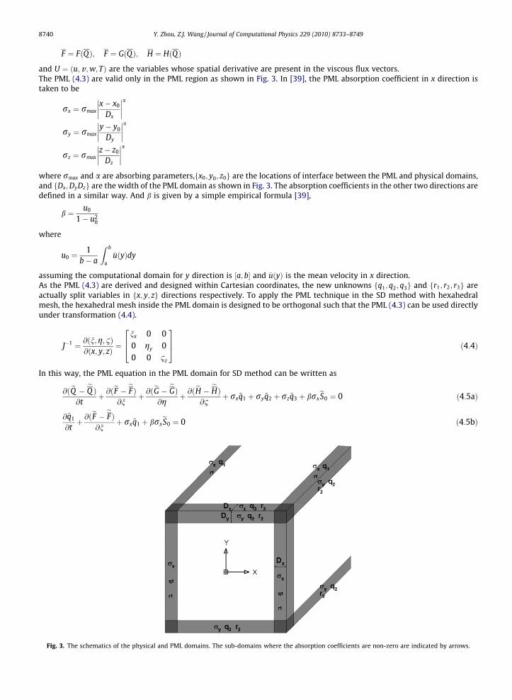
Fig.

8740 Y. Zhou, Z.J. Wang / Journal of Computational Physics 229 (2010) 8733–8749

F ¼ FðQÞ; F ¼ GðQÞ; H ¼ HðQÞ

and U ¼ ðu;v;w; TÞ are the variables whose spatial derivative are present in the viscous flux vectors.The PML (4.3) are valid only in the PML region as shown in Fig. 3. In [39], the PML absorption coefficient in x direction istaken to be

rx ¼ rmaxx� x0

Dx

���� ����ary ¼ rmax

y� y0

Dy

���� ����arz ¼ rmax

z� z0

Dz

���� ����a

where rmax and a are absorbing parameters,fx0; y0; z0g are the locations of interface between the PML and physical domains,and fDx;DyDzg are the width of the PML domain as shown in Fig. 3. The absorption coefficients in the other two directions aredefined in a similar way. And b is given by a simple empirical formula [39],

b ¼ u0

1� u20

where

u0 ¼1

b� a

Z b

a

�uðyÞdy

assuming the computational domain for y direction is ½a; b� and �uðyÞ is the mean velocity in x direction.As the PML (4.3) are derived and designed within Cartesian coordinates, the new unknowns fq1; q2; q3g and fr1; r2; r3g areactually split variables in fx; y; zg directions respectively. To apply the PML technique in the SD method with hexahedralmesh, the hexahedral mesh inside the PML domain is designed to be orthogonal such that the PML (4.3) can be used directlyunder transformation (4.4).

J�1 ¼ @ðn;g; 1Þ@ðx; y; zÞ ¼

nx 0 00 gy 00 0 1z

264375 ð4:4Þ

In this way, the PML equation in the PML domain for SD method can be written as

@ðeQ � eQ Þ@t

þ @ðeF � eF Þ@n

þ @ðeG � eGÞ@g

þ @ðeH � eHÞ@1

þ rx~q1 þ ry~q2 þ rz~q3 þ brxeS0 ¼ 0 ð4:5aÞ

@~q1

@tþ @ð

eF � eFÞ@n

þ rx~q1 þ brxeS0 ¼ 0 ð4:5bÞ

3. The schematics of the physical and PML domains. The sub-domains where the absorption coefficients are non-zero are indicated by arrows.

Y. Zhou, Z.J. Wang / Journal of Computational Physics 229 (2010) 8733–8749 8741

@~q2

@tþ @ð

eG � eGÞ@g

þ ry~q2 ¼ 0 ð4:5cÞ

@~q3

@tþ @ð

eH � eHÞ@1

þ rz~q3 ¼ 0 ð4:5dÞ

@~r1

@tþ rx~r1 ¼

@ðeU � eUÞ@n

þ brxeS1 ð4:5eÞ

@~r2

@tþ ry~r2 ¼

@ðeU � eUÞ@g

ð4:5fÞ

@~r3

@tþ rz~r3 ¼

@ðeU � eUÞ@1

ð4:5gÞ

~e1 ¼@ eU@n� rx~r1 þ brx

eS1 ð4:5hÞ

~e2 ¼@ eU@g� ry~r2 ð4:5iÞ

~e3 ¼@ eU@1� rz~r3 ð4:5jÞ

where

ðeQ � eQ Þ ¼ jJj � ðQ � QÞeS0 ¼ jJj � ðF � FÞeF � eFeG � eGeH � eH2664

3775 ¼ jJjnx 0 00 gy 00 0 1z

264375 F � F

G� G

H � H

264375

~q1 ~q2 ~q3½ � ¼ jJj � q1 q2 q3½ �~r1 ~r2 ~r3½ � ¼ jJj � r1 r2 r3½ �eS1 ¼ jJj � ðU � UÞ

In (4.5), the unknowns and the fluxes are discretized in the same way as in the SD method. As in (4.5) the inviscid and viscousfluxes keep in the same forms as in the Navier–Stokes equations (2.1), the common inviscid flux and viscous flux at the inter-faces between each two element in PML domain are computed in the same manner as the common SD method described inSection 2.

5. Numerical test

5.1. Isentropic vortex propagation

A case of isentropic vortex propagation is employed here to verify the effectiveness of ASZ and PML techniques for non-linear Euler equations. The two-dimensional nonlinear Euler equations support an advective solution of the form

qump

0BBB@1CCCA ¼

q0

U0 þ u0

V0 þ m0

p0

0BBB@1CCCA ð5:1Þ

where

q0 ¼ 1� 12 ðc� 1ÞUmax2 e

1�r2

r20

!1=ðc�1Þ

u0 ¼ �ur sin h

v 0 ¼ �ur cos h

p0 ¼ 1c 1� 1

2 ðc� 1ÞU2maxe

1�r2

r20

!1=ðc�1Þ

8>>>>>>>>>><>>>>>>>>>>:

8742 Y. Zhou, Z.J. Wang / Journal of Computational Physics 229 (2010) 8733–8749

r ¼ffiffiffiffiffiffiffiffiffiffiffiffiffiffiffiffiffiffiffiffiffiffiffiffiffiffiffiffiffiffiffiffiffiffiffiffiffiffiffiffiffiffiffiffiffiffiffiffiffiðx� UotÞ2 þ ðy� VotÞ2

qðUo;VoÞ ¼ ð0:5;0:0ÞUmax ¼ 0:5Uo ¼ 0:25ro ¼ 0:2

The Euler equations are solved with the 4th-order SD method in space and an explicit 3rd-order Runge–Kutta method intime. The entire computational domain is ½�1:5;1:5� � ½�1:5;1:5�, which includes the physical domain of½�1:0;1:0� � ½�1:0;1:0� and the remaining absorbing domain. The number of elements in the physical domain is 160 (result-ing in 2560 degrees-of-freedom), and in the absorbing domain 5 stretched elements are added in each direction. In this case,the mean flow Q is,

�q�u�m�p

0BBB@1CCCA ¼

1:00:50:01=c

0BBB@1CCCA ð5:2Þ

The performance of both ASZ and PML depends on the size of the absorbing domain and the absorption coefficient. Thereflection error can be reduced by extending the length of the absorbing domain [39,71]. Here, the length of the absorbingdomain is fixed to be 0.5 for both cases, and the effectiveness of the absorbing coefficient is tested. For both techniques, thechoices of the optimal absorbing coefficient are definitely problem dependent. Tuning the absorption coefficients for thesame problem, a bigger rmax usually generate more reflection at the interfaces for both ASZ and PML, while a smallerrmax may cause an incomplete absorbing process and the unabsorbed reflecting disturbances would also contaminate thephysical domain.

In this case, an optimal absorption coefficient is found to be rmax ¼ 0:5 for ASZ. And for PML, the optimal parameters ofabsorption coefficient in (4.3) are found be rmax ¼ 10 and a ¼ 4. The absorption of the vortex in the absorbing domain isclearly demonstrated for ASZ in Fig. 4a-c and for PML in Fig. 5a–c. In Fig. 4d–f and Fig. 5d–f, the v-velocity profiles alongy ¼ 0 at time t ¼ 2:0; 3:0 and 4.0, respectively are compared with the exact solution. It is shown that in the physical domain,the numerical solutions agree with the exact solution well for both cases. To the naked eyes, the velocity profile with PMLappears to match perfectly with the analytical solution in the physical domain, while the profile with the ASZ shows a slightdiscrepancy. The absorbing processes are different for ASZ and PML techniques. Note that in the domain of ASZ, the vortex isattenuated gradually, and the strength of the vortex becomes very small at the end of the ASZ domain, where a CBC is ap-plied. Obviously, outgoing waves will reflect at this boundary if the disturbance is not zero and of course the reflected errorwill experience the absorbing process again inside of the ASZ domain while propagating upstream. It is obvious that PML ismore efficient in absorbing the disturbances. In the PML domain, the solution decays exponentially and reduces to the meanstate of flow near the end of PML domain. Thus essentially no reflection is generated at the end of the PML domain with asimple extrapolation boundary condition.

Fig. 6 compares the L/ error (maximum error) of pressure in the physical domain computed with ASZ, PML and CBC atdifferent times of the simulations. It is shown that the error of the numerical results generated with PML is the smallest

Fig. 4. The v-velocity contours (a–c) and v-velocity profile along y = 0 (d–f) with ASZ at time y = 2.0, 3.0 and 4.0.

Fig. 5. The v-velocity contours (a–c) and v-velocity profile along y = 0 (d–f) with PML at time t = 2.0, 3.0 and 4.0.

Fig. 6. Comparison of L/ error (maximum error) of pressure.

Y. Zhou, Z.J. Wang / Journal of Computational Physics 229 (2010) 8733–8749 8743

while the error with CBC is at least one order bigger than the error with PML. The error with ASZ is between those with PMLand CBC.

5.2. 3-D acoustic pulse

The propagation of a three-dimensional nonlinear acoustic pulse in a uniform mean flow is employed to test the perfor-mance and effectiveness of absorbing boundary conditions with non-linear Navier–Stokes equations. The absorbing domainsare applied in all boundaries of the cubic physical domain. The computational results with the CBC are also presented herefor comparison. The initial condition is as follows:

q ¼ 1þ P0maxe�lnzðx2þy2þz2Þ=r20

u ¼ U0

v ¼ 0w ¼ 0q ¼ 1=cþ P0maxe�lnzðx2þy2þz2Þ=r2

0

8>>>>>><>>>>>>:ð5:3Þ

8744 Y. Zhou, Z.J. Wang / Journal of Computational Physics 229 (2010) 8733–8749

where

c ¼ 1:4; r0 ¼ 1:0; U0 ¼ 0:5; P0max ¼ 0:5:

The Reynolds number in this case is 500. The proposed reference solution Q in both the ASZ and PML is

�q�u�v�w�p

0BBBBBB@

1CCCCCCA ¼1:00:50:00:01=c

0BBBBBB@

1CCCCCCA ð5:4Þ

The physical domain is ½�10;10� � ½�10;10� � ½�10;10�with a uniform mesh of 20 elements in each coordinate direction. Forthe zonal techniques, a stretched grid with three elements is used in each coordinate direction. The 4th-order SD method andan explicit 3rd-order Runge–Kutta method are used for spatial discretization and time integration respectively. Differentabsorbing coefficients are tested for both the ASZ and PML.

Fig. 7 shows the pressure contours in the X � Y plane with CBC (a–c), ASZ (d–f) and PML (g–i) at time t ¼ 4:0; 8:0 and 12.0respectively. The absorbing coefficients used here are rmax ¼ 0:5 for ASZ and rmax ¼ 20:0 for PML. In Fig. 7, the coordinate isthe pressure, which gives a three-dimensional illustration of the pressure distribution. With CBC, obvious reflections are gen-erated at the outlet boundary and contaminate the numerical solution. In the results with ASZ technique, the pressure pulseis attenuated inside the ASZ domain but a small reflecting wave is generated at the interface. The PML technique gives thebest performance among all the three presented boundary conditions. The pressure pulse is well absorbed after entering theabsorbing domain and the reflecting disturbance is very small and invisible.

Fig. 8 compares the pressure history at point ðx; y; zÞ ¼ ð8:5;0:5;0:5Þ with a reference solution. The reference solution iscomputed in a computational domain of [�20,20] � [�20,20] � [�20,20] with the same grid size. The comparisons agreewell with the observations in Fig. 7.

5.3. Viscous flow over two cylinders

In the previous two numerical tests, it has been shown that PML gives the best performance in absorbing acoustic andvertical disturbances. In this example, the case of nonlinear vortices shed by a viscous low-Mach laminar flow over two

Fig. 7. Pressure contours with CBC (a–c), ASZ (d–f) and PML (g–i) at time t = 4.0, 8.0 and 12.0.

Fig. 8. Time history of pressure at point ðx; y; zÞ ¼ ð8:5;0:5;0:5Þ with CBC (a), ASZ (b) and PML (c).

Y. Zhou, Z.J. Wang / Journal of Computational Physics 229 (2010) 8733–8749 8745

side-by-side cylinders is presented to test the performance of the three boundary conditions with complex geometry insidethe physical domain. Fig. 9 shows the computational mesh. The physical domain is ½�10;20� � ½�10;10� with a total of 5445elements. The absorbing domain is added around the physical domain and a stretched grid with five elements is used in eachcoordinate direction. The numerical method for the spatial discretization and time integration is the same as in the previoustwo cases.

The Mach number of the uniform incoming flow is Ma ¼ 0:2 and the Reynolds number based on the diameter of the cyl-inder D is Re ¼ 200. The center-to-center spacing of the two cylinders is s ¼ 3D. The inlet flow and the initial condition of theflow field is set to be

Q 0 ¼

qu

vp

0BBB@1CCCA ¼

1:00:20:01=c

0BBB@1CCCA ð5:5Þ

Thus the proposed mean solution Q in (4.1) is the uniform flow Q ¼ Q0 as the natural choice for this problem.Optimal parameters of absorption coefficient in (15) are found be rmax ¼ 10 and a ¼ 4 for PML in this case. Fig. 10 shows

the vorticity contours at different times in the case with PML. The absorbing process of the shedding vortices can be observedin this figure from t ¼ 280 to t ¼ 330 over roughly a period. The shedding vortices are gradually absorbed as they convect outof the physical domain and enter the PML domain. Fig. 11 shows the history of v-velocity and pressure at pointðx; yÞ ¼ ð19:0;3:0Þ from time t ¼ 300 to t ¼ 600 and compares with the reference result which is obtained in a referencephysical domain ½�10;40� � ½�20;20� with PML. Excellent agreement is found, which indicates that the performance ofthe PML domain in absorbing the shedding vortices is very effective. Very good results have been achieved with the relativelysmall domain.

Fig. 12 shows the instantaneous vorticity contours in the cases with CBC and ASZ. It is noted that in current computationalmesh with CBC, the boundary condition significantly affects the flow field of the physical domain and the shedding vorticeslose the regular alignment as shown in Fig. 11. In the case with ASZ, the shedding vortices keep a similar pattern as the casewith PML and are gradually absorbed after entering the absorbing domain. In this case, an optimal parameter of absorptioncoefficient is chosen to be rmax ¼ 0:1 for ASZ.

Fig. 9. Computational mesh of viscous flow over two cylinders.

Fig. 10. Vorticity contours at time t ¼ 280;290;300;310;320 and 330 in the case with PML, from left to right, top to bottom.

8746 Y. Zhou, Z.J. Wang / Journal of Computational Physics 229 (2010) 8733–8749

Here, the authors try to investigate the effect of boundary conditions on the drag and lift forces on the wall of the cylin-ders. Fig. 13 shows the time history of the drag coefficients for the cases with different boundary conditions. It is shown thatthe Cd in the case with PML agrees well with the reference results, as shown in Fig. 13(a). The current computational domainis much smaller than those used in previously published paper [17,46], and with the current mesh the boundary conditionsignificantly affects the drag and lift forces in the cases with CBC and ASZ, as shown in Fig. 13(b). The Cd with CBC is highlyoscillatory owing to the high frequency disturbances generated at the outflow boundary, while the Cd with ASZ is smooth butmuch higher than the results with PML. In [17], the outflow boundary is set to be far downstream of the cylinders with muchlarger spaced grid to dissipate the disturbances. Table 1 compares the averaged Cd of the current cases with the result in

Fig. 11. Time history of v-velocity (a) and pressure (b) at point ðx; yÞ ¼ ð19:0;3:0Þ from time t ¼ 300 to t ¼ 600 in the case with PML.

Fig. 12. Instantaneous vorticity contours in the cases with CBC (a) and ASZ (b).

Fig. 13. Time history of drag coefficients, (a) PML and the reference; (b) ASZ and CBC.

Y. Zhou, Z.J. Wang / Journal of Computational Physics 229 (2010) 8733–8749 8747

Table 1Comparison of mean drag coefficients for flow over two cylinders at Re ¼ 200 and s ¼ 3D.

CBC ASZ PML Liang et al. Ding et al.

Cd 1.530 1.650 1.492 1.496 1.548

8748 Y. Zhou, Z.J. Wang / Journal of Computational Physics 229 (2010) 8733–8749

[17,46]. The current results with PML agree well with the result of Liang et al. [17] and the SD method is also used in theircase.

6. Conclusions

Two popular absorbing boundary conditions, the absorbing sponge zone and perfectly matched layer, are implementedwith the spectral difference method on hexahedral meshes for non-linear Euler and Navier–Stokes equations in this paper.The disturbances are gradually attenuated thus the reflection at the end of the absorbing domain is minimized by using thespectral difference method with both zonal techniques. Both the ASZ and PML perform very effectively in the vortex andacoustic propagation problems. The reflected errors with the two zonal techniques are much smaller than those with theCBC based on linearized one-dimensional Euler equations. The absorbing processes with the two techniques are differentowing to the different design concepts. The formula of the ASZ is much simpler than the PML technique and therefore easierto implement. However, it is still somewhat reflective and generates visible reflections at the interface with the ASZ betweenthe physical domain and the absorbing domain. PML is more efficient in absorbing the disturbances. With the PML technique,the magnitude of the disturbances decreases exponentially in the absorbing domain and the solution finally reduces to theproposed mean solution at the end of the absorbing domain while the reflection generated at the interface between thephysical domain and absorbing domain is almost invisible. In the case of low-Mach number laminar flow past two side-by-side cylinders, with complex geometries inside the physical domain the PML technique also performs well in absorbingthe shedding vortices and accurately predicts the drag and lift forces on the wall with a relatively small computationaldomain.

Acknowledgements

The authors would like to acknowledge the support for this work from the Department of Aerospace Engineering, IowaState University, and partial support by the Air Force Office of Scientific Research.

References

[1] R. Abgrall, P.L. Roe, High order fluctuation schemes on triangular meshes, J. Sci. Comput. 19 (2003) 3–36.[2] S. Abarbanel, D. Gottlieb, A mathematical analysis of the PML method, J. Comput. Phys. 154 (1997) 266–283.[3] S. Abarbanel, D. Stanescu, M.Y. Hussaini, Unsplit variable perfectly matched layers for the shallow water equation with coriolis forces, Comput. Geosci.

7 (4) (2003) 265–294.[4] B. Bacache, S. Fauqueus, P. Joly, Stability of perfectly matched layers, group velocities and anisotropic waves, J. Comput. Phys. 188 (2003) 399–433.[5] E. Bacache, A.-S. Bonnet-Ben Dhia, G. Legendre, Perfectly matched layers for the convected Helmholtz equations, SIAM J. Numer. Anal. 42 (1) (2004)

409–433.[6] T.J. Barth, P.O. Frederickso, High-order solution of the Euler equations on unstructured grids using quadratic reconstruction, AIAA Paper 96-0027, 1996.[7] F. Bassi, S. Rebay, High-order accurate discontinuous finite element solution of the 2D euler equations, J. Comput. Phys. 138 (1997) 251–285.[8] A. Bayliss, E. Turkel, Radiation boundary conditions for wave-like equations, Comm. Pure. Appl. Math. 33 (1980) 707–725.[9] A. Bayliss, M. Gunzburger, E. Turkel, Boundary conditions for the numerical solution of elliptic equations in exterior regions, SIAM J. Appl. Math. 42

(1982) 430–451.[10] J.-P. Berenger, A perfectly matched layer for the absorption of electromagnetic wave, J. Comput. Phys. 144 (1994) 185–200.[11] D.J. Bodony, analysis of sponge zones for computational aeroacoustics, J. Comput. Phys. 212 (2006) 681–702.[12] B. Cockburn, C.W. Shu, TVB Runge–Kutta local projection discontinuous Galerkin finite element method for conservation laws II: general framework,

Math. Comput. 52 (1989) 411–435.[13] B. Cockburn, C.W. Shu, The Runge–Kutta discontinuous Galerkin method for conservation laws V: multidimensional systems, J. Comput. Phys. 141

(1998) 199–224.[14] F. Collino, P. Monk, The perfectly matched layer in curvilinear coordinates, SIAM J. Sci. Comp. 19 (6) (1998) 2016.[15] T. Colonius, S.K. Lele, P. Moin, Boundary condition for direct computation of aerodynamic sound generation, AIAA J. 31 (9) (1993) 1574–1582.[16] T. Colonius, Modelling artificial boundary conditions for compressible flow, Ann. Rev. Fluid Mech. 36 (2004) 315–345.[17] H. Ding, C. Shu, K.S. Yeo, D. Xu, Numerical simulation of flows around two circular cylinders by mesh-free least square-based finite difference methods,

Int J. Numer. Meth. Fluids 53 (2007) 305–332.[18] B. Engquist, A. Majda, Absorbing boundary conditions for the numerical evaluation of waves, Math. Comp. 31 (139) (1977) 629–651.[19] J.B. Freund, Proposed inflow/outflow boundary condition for direct computation of aerodynamic sound, AIAA J. 35 (4) (1997) 740–742.[20] S.D. Gedney, An anisotropic perfectly matched layer-absorbing medium for the truncation of FDTD lattices, IEEE Trans. Antennas Propagation 44

(1996) 1630.[21] M.B. Giles, Non-reflecting boundary conditions for Euler equation calculations, AIAA J. 28 (1990) 2050–2058.[22] J.S. Hesthaven, On the analysis and construction of perfectly matched layers for the linearized Euler equations, J. Comput. Phys. 142 (1998) 129–147.[23] T. Hagstrom, I. Nazarov, Absorbing layers and radiation boundary conditions for jet flow simulations, AIAA Paper 2002-2606, 2002.[24] T. Hagstrom, I. Nazarov, Perfectly matched layers and radiation boundary conditions for shear flow calculations, AIAA Paper 2003-3298, 2003.[25] R.L. Higdon, Absorbing boundary conditions for difference approximations to the muti-dimensional wave equation, Math. Comp. 47 (176) (1986) 437–

459.

Y. Zhou, Z.J. Wang / Journal of Computational Physics 229 (2010) 8733–8749 8749

[26] C. Hirsch, Numerical Computation of Internal and External Flows: Fundamentals of Computational Fluid Dynamics, second ed., Butterworth-Heinemann, 2007, pp. 607–609.

[27] C. Hu, C.W. Shu, Weighted essentially non-oscillatory schemes on triangular meshes, J. Comput. Phys. 150 (1999) 97–127.[28] F.Q. Hu, On absorbing boundary conditions for linearized Euler equations by a perfectly matched layer, J. Comput. Phys. 129 (1996) 201–219.[29] F.Q. Hu, On Perfectly Matched Layer as an absorbing boundary condition, AIAA Paper 96-1664, 1996.[30] F.Q. Hu, J.L. Manthey, Application of PML absorbing boundary conditions to the Benchmark Problems of Computational Aeroacoustics, NASA CP 3352,

in: Second Computational Aeroacoustics (CAA) Workshop on Benchmark Problems, 1997, pp. 119–151.[31] F.Q. Hu, A stable, Perfectly matched layer for linearized Euler equations in unsplit physical variables, J. Comput. Phys. 173 (2001) 455–480.[32] F.Q. Hu, On Constructing stable Perfectly Matched Layers as an absorbing boundary condition for Euler equations, AIAA Paper 2002-0227, 2002.[33] F.Q. Hu, Solution of aeroacoustic benchmark problems by discontinuous Galerkin method and Perfectly Matched Layer for nonuniform mean flows, in:

the Proceedings of the 4th CAA Workshop on Benchmark Problems, NASA/CP-2004-212954, 2004.[34] F.Q. Hu, Absorbing boundary conditions (a review), Int. J. Comput. Fluid Dyn. 18 (6) (2004) 513–522.[35] F.Q. Hu, On using Perfectly Matched Layer for the Euler equations with a non-uniform mean flow, AIAA-Paper 2004-2966, 2004.[36] F.Q. Hu, A perfectly matched layer absorbing boundary condition for linearized Euler equations with a non-uniform mean flow, J. Comput. Phys. 208

(2005) 469–492.[37] F.Q. Hu, On the construction of PML absorbing boundary condition for the non-linear Euler equations, AIAA Paper 2006-0798, 2006.[38] F.Q. Hu, X.D. Li, D.K. Lin, PML absorbing boundary condition for non-linear aeroacoustics problems, AIAA Paper 2006-2521, 2006.[39] F.Q. Hu, X.D. Li, D.K. Lin, Absorbing boundary conditions for nonlinear Euler and Navier–Stokes equations based on the Perfectly Matched Layer

technique, J. Comput. Phys. 227 (9) (2008) 4398–4424.[40] P.G. Huang, Z.J. Wang, Y. Liu, An implicit space-time spectral difference method for discontinuity capturing using adaptive polynomials, AIAA Paper

2005-5255, 2005.[41] H.T. Huynh, A flux reconstruction approach to high-order schemes including discontinuous Galerkin methods, AIAA Paper 2007-4079.[42] A. Jameson, A Proof of the stability of the spectral difference method for all orders of accuracy, ACL Report No. 2009-1, Stanford University, March,

2009.[43] D.A. Kopriva, J.H. Kolias, A conservative staggered-grid Chebyshev multidomain method for compressible flows, J. Comput. Phys. 125 (1996) 244–261.[44] D.A. Kopriva, A staggered-grid multidomain spectral method for compressible Navier–Stokes equations, J. Comput. Phys. 143 (1998) 125–158.[45] A. Lerat, J. Sides, V. Daru, Efficient computation of steady and unsteady transonic flows by an implicit solver, in: W.G. Habashi (Ed.), Advances in

Computational Transonics, Pineridge Press, 1984.[46] C.L. Liang, S. Premasuthan, A. Jameson, High-order accurate simulation of low-Mach laminar flow past two side-by-side cylinders using spectral

difference method, Comput. Struct. 87 (2009) 812–827.[47] Y. Liu, M. Vinokur, Z.J. Wang, discontinuous spectral difference method for conservation laws on unstructured grids, in: C. Groth, D.W. Zingg (Eds.),

Proceeding of the Third International Conference in CFD, Toronto, Springer, 2004, pp. 449–454.[48] Y. Liu, M. Vinokur, Z.J. Wang, Spectral (finite) difference method for conservation laws on unstructured grids I: basic formulation, J. Comput. Phys. 216

(2006) 780–801.[49] Y. Liu, M. Vinokur, Z.J. Wang, Spectral (finite) volume method for conservation laws on unstructured grids V: extension to three-dimensional systems,

J. Comput. Phys. 212 (2006) 454–472.[50] G. May, A. Jameson, A spectral difference method for the Euler and Navier–Stokes equations on unstructured grids, AIAA Paper 2006-304, 2006.[51] A.T. Patera, A spectral element method for fluid dynamics: Laminar flow in a channel expansion, J. Comput. Phys. 54 (1984) 468–488.[52] S.A. Parrish, F.Q. Hu, Application of PML absorbing boundary condition to aeroacoustics problems with an oblique mean flow, AIAA Paper 2007-3509,

2007.[53] P.G. Petropoulos, Reflectionless sponge layers as absorbing boundary conditions for the numerical solution of Maxwell’s equations in rectangular,

cylindrical and spherical coordinates, SIAM J. Appl. Math. 60 (2000).[54] T. Poinsot, S.K. Lele, Boundary conditions for direct simulation of compressible viscous flows, J. Comput. Phys. 101 (1992) 104–129.[55] P.L. Roe, Approximate Riemann solvers, parameter vectors, and difference schemes, J. Comput. Phys. 43 (1981) 357–372.[56] Y. Sun, Z.J. Wang, Y. Liu, Spectral (finite) volume method for conservation laws on unstructured grids VI: extension to viscous flow, J. Comput. Phys. 215

(2006) 41–58.[57] Y. Sun, Z.J. Wang, Y. Liu, High-order multidomain spectral difference method for the Navier–Stokes equations on unstructured hexahedral grids,

Commun. Comput. Phys. 2 (2) (2007) 310–333.[58] Y. Sun, Z.J. Wang, Y. Liu, C.L. Chen, Efficient implicit LU-SGS algorithm for high-order spectral difference method on unstructured hexahedral grids,

AIAA Paper, 2007-0313, 2007.[59] S. Ta’asan, D.M. Nark, An absorbing buffer zone technique for acoustic wave propagation, AIAA J. 95 (0164) (1995).[60] C.K.W. Tam, L. Auriault, F. Cambulli, Perfectly Matched Layer as an absorbing boundary condition for the linearized Euler equations in open and ducted

domains, J. Comput. Phys. 144 (1998) 213–234.[61] K.W. Thompson, Time-dependent boundary conditions for hyperbolic systems, J. Comput. Phys. 68 (1987) 1–24.[62] E. Turkel, A. Yefet, Absorbing PML boundary layers for wave-like equations, Appl. Numer. Math. 27 (1998) 533–557.[63] K. Van den Abeele, C. Lacor, Z.J. Wang, On the stability and accuracy of the spectral difference method, J. Sci. Comput. 37 (2008) 162–188.[64] Z.J. Wang, Spectral (finite) volume method for conservation laws on unstructured grids: basic formulation, J. Comput. Phys. 178 (2002) 210–251.[65] Z.J. Wang, Y. Liu, Spectral (finite) volume method for conservation laws on unstructured grids III: extension to one-dimensional systems, J. Sci. Comput.

20 (2004) 137–157.[66] Z.J. Wang, L. Zhang, Y. Liu, Spectral (finite) volume method for conservation laws on unstructured grids III: extension to two-dimensional systems, J.

Sci. Comput. 194 (2004) 716–741.[67] Z.J. Wang, Y. Liu, The spectral difference method for the 2D Euler equations on unstructured grids, AIAA Paper 2005-5112, 2005.[68] Z.J. Wang, Y. Liu, G. May, A. Jameson, Spectral difference method for unstructured grids II: extension to the Euler equations, J. Sci. Comput. 32 (1) (2007)

45–71.[69] H.C. Yee, R.M. Beam, R.F. Warming, Boundary approximation for implicit schemes for one-dimensional inviscid equation of gas dynamics, AIAA J. 20

(1982) 1203–1211.[70] L. Zhao, A.C. Cangellaris, GT-PML: generalized theory of Perfectly Matched Layers and its application to the reflectionless truncation of finite-difference

time-domain grids, IEEE Trans. Microwave Theory Tech. 44 (1996) 2555–2563.[71] Y. Zhou, Z.J. Wang, Simulation of CAA benchmark problems using high-order spectral difference method and Perfectly Matched layers, AIAA-2010-838.