rspa.royalsocietypublishing.org

Research

Article submitted to journal

Subject Areas:

mathematical modelling

Keywords:

advection, Taylor–Aris dispersion,

rivulet

Author for correspondence:

S. K. Wilson

e-mail: s.k.wilson@strath.ac.uk

Advection and Taylor–Aris

dispersion in rivulet flow

F. H. H. Al Mukahal1,2, B. R. Duffy1 and

S. K. Wilson1

1Department of Mathematics and Statistics, University

of Strathclyde, Livingstone Tower, 26 Richmond Street,

Glasgow G1 1XH, United Kingdom2Department of Mathematics and Statistics, King

Faisal University, P.O. Box 400, Hafouf 31982,

Kingdom of Saudi Arabia

Motivated by the need for a better understanding

of the transport of solutes in microfluidic flows

with free surfaces, the advection and dispersion of

a passive solute in steady unidirectional flow of a

thin uniform rivulet on an inclined planar substrate

driven by gravity and/or a uniform longitudinal

surface shear stress are analysed. Firstly, we describe

the short-time advection of both an initially semi-

infinite and an initially finite slug of solute of uniform

concentration. Secondly, we describe the long-time

Taylor–Aris dispersion of an initially finite slug of

solute. In particular, we obtain the general expression

for the effective diffusivity for Taylor–Aris dispersion

in such a rivulet, and discuss in detail its different

interpretations in the special case of a rivulet on a

vertical substrate.

1. Introduction

One of the ongoing challenges in microfluidics is that

of controlling and optimising the transport (i.e. the

mixing and dispersion) of solutes at small length scales

and low Reynolds numbers (see, for example, the

reviews by Stone, Stroock and Ajdari [1], Darhuber

and Troian [2], and Lee et al. [3]). The dispersion

(i.e. the combined effect of advection and diffusion)

of a solute in a steadily flowing fluid is a classical

problem in fluid mechanics which arises in numerous

practical situations (such as, for example, the spread of

pollutants in rivers, chromatographic separation, and the

transport of dissolved drugs in the bloodstream) and

has been the subject of a huge body of theoretical and

experimental research, the vast majority of it originating

from the pioneering papers by Taylor [4,5] and Aris

c© The Author(s) Published by the Royal Society. All rights reserved.

2

rspa.ro

yals

ocie

typublis

hin

g.o

rgP

roc

RR

oc

A0000000

..........................................................

[6] published in this journal. The key insight of this pioneering work was that after a sufficiently

long time the mean concentration of solute adopts a symmetric Gaussian distribution which

moves downstream with the mean speed of the flow and spreads in the flow direction with an

effective (or enhanced) diffusion coefficient, Deff , which is larger than the molecular diffusion

coefficient, D, due to the presence of the flow. This phenomenon is now known as Taylor–

Aris (or sometimes simply just Taylor) dispersion. In the simplest case of Poiseuille flow in

a pipe of circular cross-section with diameter d, Taylor [4] obtained the famous expression

Deff =D(1 + Pe2con/192), where Pecon = ud/D is the conventional Péclet number based on the

mean velocity over the cross-section of the pipe, u. As Witelski and Bowen [7, Chap. 11] say,

“Taylor’s original paper was presented in his unique and very physically intuitive style; it is

deceptively short and challenging to follow”, and subsequently many authors have sought to

formalise Taylor’s argument using a variety of methods, including the method of moments (Aris

[6]), Fourier series (Lungu and Moffatt [8]), the method of multiple scales (Pagitsas, Nadim and

Brenner [9], Zhang and Frigaard [10]), centre-manifold theory (Mercer and Roberts [11], Young

and Jones [12], Balakotaiah and Chang [13]), and Liapunov–Schmidt reduction (Ratnakar and

Balakotaiah [14]). There is now an extensive literature on dispersion in channels with a variety

of cross-sectional shapes (see, for example, Brenner and Edwards [15], Dutta and Leighton [16],

Dutta, Ramachandran and Leighton [17], and Dutta [18]), and, in particular, a body of work on

dispersion in wide channels (see, for example, Doshi, Daiya and Gill [19], Chatwin and Sullivan

[20], Pagitsas, Nadim and Brenner [9], Guell, Cox and Brenner [21], Smith [22,23], and Ajdari,

Bontoux and Stone [24]). However, with the notable exception of the work of Darhuber et al. [25]

on mixing in thermocapillary flows on micropatterned surfaces, there has been surprisingly little

theoretical work on transport of solutes in microfluidic flows with free surfaces and, in particular,

on the topic of the present contribution, namely the dispersion of a passive solute in a rivulet flow.

While the present work is primarily motivated by and described in the context of the dispersion

of a solute, the present results also apply to the transport of heat with insulating boundary

conditions and can readily be extended to other thermal boundary conditions (see, for example,

Lungu and Moffatt [8]), and so the present work is also relevant to the wide range of practical

situations involving heat transfer in the presence of rivulets (see, for example, Kabov [26] and

Kabov, Bartashevich and Cheverda [27]).

In addition to in microfluidics, rivulets of many different fluids occur in a wide variety of other

practical contexts, including heat exchangers, trickle-bed reactors and various coating processes,

and as a result there has been considerable theoretical work on locally unidirectional rivulet flow

(see, for example, Paterson, Wilson and Duffy [28] and the references therein). In particular, Young

and Davis [29], Duffy and Moffatt [30], Myers, Liang and Wetton [31], Saber and El-Genk [32],

Wilson and Duffy [33], Sullivan, Wilson and Duffy [34], Benilov [35], Tanasijczuk, Perazzo and

Gratton [36], Wilson, Sullivan and Duffy [37], and Herrada et al. [38] considered various aspects

of locally unidirectional rivulet flow and its stability.

In the present contribution we analyse advection and dispersion of a passive solute in steady

unidirectional flow of a thin uniform rivulet on an inclined planar substrate driven by gravity

and/or a uniform longitudinal surface shear stress. In particular, we obtain the general expression

for the effective diffusivity Deff for Taylor–Aris dispersion in such a rivulet, and discuss in detail

its different interpretations in the special case of a rivulet on a vertical substrate.

2. Rivulet flow

Consider steady unidirectional flow of a thin uniform rivulet of incompressible Newtonian fluid

on a planar substrate inclined at an angle α (0≤ α≤ π) to the horizontal, the flow being driven

by gravity and/or a uniform longitudinal surface shear stress τ . Aspects of this flow problem

were described by Wilson and Duffy [33] and Sullivan [34]; here we present only the key results

relevant to the present study of advection and Taylor–Aris dispersion of a passive solute in such

a flow.

3

rspa.ro

yals

ocie

typublis

hin

g.o

rgP

roc

RR

oc

A0000000

..........................................................

O

x

y

z

g

τa

−a

β

β

α

Free surfacez = h(y)

Substratez = 0

Figure 1. Sketch of the geometry of the problem: steady unidirectional flow of a thin uniform rivulet of incompressible

Newtonian fluid on a planar substrate inclined at an angle α (0≤ α≤ π) to the horizontal and subject to a uniform

longitudinal surface shear stress τ .

Referred to a Cartesian coordinate system Oxyz with Ox down the line of greatest slope and

Oz normal to the substrate at z = 0, as shown in Fig. 1, we scale and nondimensionalise variables

according to

y= ℓy∗, z = ǫℓz∗, a= ℓa∗, h= ǫℓh∗, β = ǫβ∗, A= ǫℓ2A∗,

u=Uu∗, p= pa + ǫρgℓp∗, τ = ǫρgℓτ∗, Q= ǫUℓ2Q∗, u=Uu∗,(2.1)

where u= u(y, z)i and p are the fluid velocity and pressure, ℓ= (γ/ρg)1/2 is the capillary length,

z = h(y) denotes the free surface of the rivulet, ǫ (≪ 1) is the aspect ratio of the cross-section of the

rivulet, a and A are the semi-width and cross-sectional area of the rivulet, β denotes the contact

angle, µ and ρ are the constant viscosity and density of the fluid, U = ǫ2ρgℓ2/µ is the velocity

scale associated with gravity-driven flow, g is gravitational acceleration, Q is the volume flux of

fluid down the rivulet, u is the mean velocity over the cross-section, γ is the coefficient of surface

tension, and pa is atmospheric pressure. Then, with the superscript stars dropped for clarity, the

governing Navier–Stokes equation gives, at leading order in ǫ,

uzz =− sinα, py = 0, pz =− cosα, (2.2)

which are to be integrated subject to the boundary conditions

u= 0 on z = 0, uz = τ and p=−h′′ on z = h, (2.3)

where a prime denotes differentiation with respect to argument. Thus

p= (h− z) cosα− h′′, u=sinα

(2hz − z2

)

2+ τz, (2.4)

4

rspa.ro

yals

ocie

typublis

hin

g.o

rgP

roc

RR

oc

A0000000

..........................................................

in which h satisfies

(h′′ − h cosα)′ = 0, (2.5)

to be integrated subject to the contact-line conditions

h= 0, h′ =∓β at y=±a. (2.6)

Therefore

Q=

∫a−a

∫h0

u dz dy=sinα I3

3+τI22, u=

Q

A=

sinα I33I1

+τI22I1

, (2.7)

where we have defined I1 (=A), I2 and I3 by

In =

∫a−a

hn dy (n= 1, 2, 3). (2.8)

In Appendix A we provide the solution of equations (2.5)–(2.6) for h, as well as explicit

expressions for the quantities I1, I2 and I3 defined in (2.8) and appearing in the expressions forQ

and u given in (2.7). In general, for given values of α and τ , any two of the four quantities a, β, Q

and the maximum thickness hm = h(0) may be prescribed. (In practice, it is difficult to prescribe

hm and so, for brevity, we will not consider this situation further in the present work.)

The maximum and minimum fluid velocities over the rivulet, which we denote by umax

and umin, respectively, satisfy umax ≥ 0 and umin ≤ 0. When τ ≥ 0 (i.e. when the surface shear

stress acts in the same direction as gravity) the velocity is downwards everywhere (i.e. u≥ 0

throughout the rivulet), umax = hm(hm sinα+ 2τ)/2 occurs at the apex of the rivulet (i.e. at

y= 0, z = hm) and umin = 0 occurs on the substrate z = 0, but when τ < 0 (i.e. when the surface

shear stress opposes gravity) the velocity is upwards (i.e. u< 0) near the edges of the rivulet,

but can be downwards elsewhere. In particular, when τ ≤−hm sinα the velocity is upwards

throughout the rivulet with umax = 0 and umin = hm(hm sinα+ 2τ)/2 occurring at the apex

of the rivulet, but when −hm sinα< τ < 0 there is a region of downwards flow in the centre

of the rivulet with umax = (hm sinα+ τ)2/(2 sinα) occurring within this region at y= 0, z =

(hm sinα+ τ)/ sinα and umin =−τ2/(2 sinα) occurring on the free surface z = h at the positions

at which h sinα+ τ = 0. For future reference note that the flux Q (and hence the mean velocity u)

are positive for τ > τc, zero for τ = τc and negative for τ < τc, where the critical value τ = τc (< 0)

corresponding to no net flow is given by τc =−2 sinα I3/(3I2). Note that Wilson and Duffy [33]

and Sullivan et al. [34] give a complete description of the cross-sectional flow patterns in the

special cases of a vertical substrate (i.e. when α= π/2) and a perfectly wetting fluid (i.e. when

β = 0), respectively.

The special case of purely gravity-driven-flow corresponds simply to τ = 0, in which case the

velocity is downwards everywhere with umax = h2m sinα/2 and umin = 0.

On the other hand, the special case of purely surface-shear-stress-driven flow may be obtained

by taking the limit |τ | →∞ with u rescaled as u= τ u to give simply u= z; then the rescaled flux

Q=Q/τ and the rescaled mean velocity u= u/τ satisfy Q→ I2/2 and u→ I2/(2I1), respectively,

and the rescaled minimum and maximum velocities are umax = umax/τ → hm and umin =

umin/τ → 0, again occurring at the apex and on the substrate, respectively.

In the special case of flow on a vertical substrate (i.e. when α= π/2) the solution of equations

(2.5)–(2.6) is simply the parabolic profile

h= hm

(1− y2

a2

), hm =

aβ

2, (2.9)

so that

I1 =A=4ahm3

, I2 =16ah2m15

, I3 =32ah3m35

, (2.10)

and therefore

Q=32ah3m105

+8τah2m15

, u=3Q

4ahm=

8h2m35

+2τhm5

. (2.11)

5

rspa.ro

yals

ocie

typublis

hin

g.o

rgP

roc

RR

oc

A0000000

..........................................................

For future reference, note that in this case when τ ≥ 0 then umax = aβ(aβ + 4τ)/8, when τ ≤−aβ/2 then umin = aβ(aβ + 4τ)/8, and when −aβ/2< τ < 0 then umax = (aβ + 2τ)2/8 at y= 0,

z = (aβ + 2τ)/2 and umin =−τ2/2 at y=±(a(aβ + 2τ)/β)1/2, z =−τ , and τc =−2aβ/7.

3. Dispersion of a passive solute in a rivulet

If a passive solute is released into the rivulet then it disperses (that is, it is advected by the flow and

diffuses), and its concentration c= c(x, y, z, t), where t denotes time, satisfies the (dimensional)

advection–diffusion equation

ct + ucx =D(cxx +∇2c

), (3.1)

where D is the diffusivity, and ∇2 denotes the two-dimensional Laplacian given by

∇2 =∂2

∂y2+

∂2

∂z2. (3.2)

Also c satisfies the no-flux boundary conditions

n · ∇c= 0 on z = 0 and z = h, (3.3)

where n denotes the unit outward normal to the boundary of the fluid (comprising the substrate

and free surface). In addition, we assume that the solute is released at some initial instant t= 0

with a prescribed initial distribution c(x, y, z, 0), occupying a (possibly infinite) portion x1 ≤ x≤x2 of the rivulet, with x1 and x2 prescribed.

A key quantity of interest is the mean concentration over the cross-section, which we denote

by c= c(x, t), and which is defined by

c=1

A

∫a−a

∫h0

c dz dy. (3.4)

Also the mean initial concentration over x1 ≤ x≤ x2, which we denote by C0, is defined by

C0 =1

x2 − x1

∫x2

x1

c(x, 0) dx, (3.5)

the integral here being interpreted as an appropriate limit if x2 − x1 is infinite.

4. Advection of a passive solute in a rivulet

At sufficiently short times after the solute is released, specifically for t≪ ℓ2/D, advection

dominates over diffusion, and so the effects of diffusion are negligible. In this case the governing

equation for c therefore reduces simply to the advection equation ct + ucx = 0, which has solution

c(x, y, z, t) = c(x− u(y, z)t, y, z, 0), reflecting the fact that the particle of solute that is at position

r= r0 at t= 0 is at r= r0 + uti at time t. Note that the behaviour of u described in Section

2 immediately implies that when τ ≥ 0 all of the solute is advected downwards, when τ ≤−hm sinα all of the solute is advected upwards, and when −hm sinα< τ < 0 both downwards

and upwards advection occur and, in particular, when τ = τc the net advection is zero.

We non-dimensionalise and scale variables as in (2.1), together with

x= ℓx∗, t=ℓ

Ut∗, c=C0c

∗, c=C0c∗, (4.1)

where C0 is defined in (3.5); again we drop the superscript stars for clarity.

(a) A semi-infinite slug of solute

First we consider the situation in which the solute initially takes the form of a semi-infinite slug

of uniform concentration c0 in x≤ 0, where c0 is a constant, i.e. c= c0 if x≤ 0 and c= 0 if x> 0.

In his pioneering paper, Taylor [4] considered advection of such a slug in Poiseuille flow in a pipe

6

rspa.ro

yals

ocie

typublis

hin

g.o

rgP

roc

RR

oc

A0000000

..........................................................

of circular cross-section, for which he showed that the mean concentration c is piecewise linear in

the distance x down the pipe, specifically c= c0 for x< 0, c= c0[1− (x/umaxt)] for 0≤ x≤ umaxt,

and c= 0 for x> umaxt. Note that there is nothing generic about this piecewise-linear dependence

of c on x. For example, the corresponding calculation for two-dimensional Poiseuille flow yields

c= c0[1− (x/umaxt)]1/2 for 0≤ x≤ umaxt, i.e. a square root dependence on x. However, the “self-

similar” dependence on x and t in the combination x/t is generic for this problem.

For rivulet flow, with C0 = c0, the (dimensionless) solution for c at time t is simply c= 1 if x≤ut and c= 0 if x> ut, the slug having a “front” at x= ut, which is planar at t= 0 but is curved for

t > 0; of course, since there is no slip at the substrate, the “base” of the front at x= 0, z = 0 remains

stationary for all t. From (3.4), c at any station x and time t is the fraction of the cross-sectional

area for which u(y, z)≥ x/t, which is of the self-similar form1

c=

1 if x< umint,

f

(x

umt

)if umint≤ x≤ umaxt,

0 if x> umaxt,

(4.2)

where um is defined by um = umax − umin (> 0), and the function f , which is determined by (3.4),

satisfies 0≤ f(x/umt)≤ 1, with f(umax/um) = 0 and f(umin/um) = 1.

Figure 2 shows the solution (4.2) for c in a rivulet on a vertical substrate plotted as a function

of x for several values of τ at time t= 1, with a= 1 and β = 1, illustrating clearly the advective

effects of the flow for both positive and negative values of τ . (Note that because of the self-similar

form of (4.2), plots of c at any other time t > 0 will be the same as those in Fig. 2 except that in

each case the x coordinate must be stretched by the amount umt.) When τ ≥ 0 all of the solute is

advected downwards, and therefore c= 1 and hence c= 1 for x≤ 0 for all t, which, in particular,

explains why the curves for such cases in Fig. 2 all pass through x= 0 and c= 1. Similarly, when

τ ≤−aβ/2 =−1/2 all of the solute is advected upwards, and therefore c= 0 and hence c= 0 for

x≥ 0 for all t, which, in particular, explains why the curves for such cases in Fig. 2 all pass through

x= 0 and c= 0. Figure 2 also includes a curve for the critical value τ = τc =−2/7 (shown dotted)

for which the net advection is zero.

In principle, a complete list of the forms that the function f in (4.2) takes for different values of

τ and α could be constructed, but it would be unwieldy, partly because, when τ < 0, several

different forms of the velocity contour u= x/t must be considered, each of which leads to a

different form for f , and partly because it seems that, in general, the integral in (3.4) is not

available in closed form when the substrate is not vertical (i.e. when α 6= π/2), the free surface

then having one of the non-parabolic profiles given in (A.1). However, in Appendix B we give

explicit expressions for f in (4.2) in two cases in which u≥ 0 everywhere, namely flow on a

vertical substrate with τ ≥ 0 and purely surface-shear-stress-driven flow; in both of these cases

f decreases monotonically from the value 1 at x= 0 to the value 0 at x= umaxt.

(b) A finite slug of solute

Now we consider the situation in which the solute initially takes the form of a finite slug of

uniform concentration c0 in 0≤ x≤∆, where c0 and ∆ are constants, i.e. c= c0 if 0≤ x≤∆ and

c= 0 if x< 0 or x>∆. Again Taylor [4] considered advection of such a slug in Poiseuille flow in a

pipe of circular cross-section, for which he again showed that c is piecewise linear in the distance

x down the pipe.

For rivulet flow, with C0 = c0 again, the (dimensionless) solution for c at time t is simply c= 0

if x≤ ut or x> ut+∆ and c= 1 if ut < x≤ ut+∆, the slug in this case having both a front at

1 The results (4.2) and (4.3)–(4.4) for advection in rivulet flow are, with appropriate re-interpretations of U and ℓ, also valid for

advection of the corresponding slugs in unidirectional flow in a channel of arbitrary cross-section, and thus they generalise

the results of Taylor [4] concerning advection in a pipe of circular cross-section.

7

rspa.ro

yals

ocie

typublis

hin

g.o

rgP

roc

RR

oc

A0000000

..........................................................

−0.3 −0.2 −0.1 0.1 0.2 0.3

0.5

1

x

c

τ = −3

τ = 2

Figure 2. Mean concentration c in advection in a rivulet on a vertical substrate in the case when the solute initially takes

the form of a semi-infinite slug of uniform concentration with c= 1 if x≤ 0 and c= 0 if x> 0 (shown dashed) given by

(4.2) plotted as a function of x for τ =−3, −17/6, −8/3, . . . , 2 and τ = τc =−2/7 (shown dotted) at time t= 1, with

a= 1 and β = 1 in each case.

x= ut+∆ and a rear at x= ut. The solution for c at time t is given by

c=

0 if x≤ umint,

1− f

(x

umt

)if umint < x≤ umaxt,

1 if umaxt < x≤∆+ umint,

f

(x−∆

umt

)if ∆+ umint < x≤∆+ umaxt,

0 if x>∆+ umaxt

(4.3)

when t≤∆/um (that is, up to the instant when the point of the rear of the slug at which the

velocity is a maximum and the point of the front of the slug at which the velocity is a minimum

first reach the same x value), and by

c=

0 if x≤ umint,

1− f

(x

umt

)if umint < x≤∆+ umint,

f

(x−∆

umt

)− f

(x

umt

)if ∆+ umint < x≤ umaxt,

f

(x−∆

umt

)if umaxt < x≤∆+ umaxt,

0 if x>∆+ umaxt

(4.4)

when t >∆/um, the function f in (4.3) and (4.4) being the same as that in (4.2).

Up to the instant t=∆/um, c increases monotonically with x up to its maximum value 1, which

is its value on a decreasing interval lying within 0≤ x≤∆, and decreases monotonically with x to

the right of this interval. At t=∆/um the interval has shrunk to a point at x= (umax/um)∆, and

thereafter c satisfies c < 1 everywhere, and can develop additional non-monotonic dependence

on x beyond what it inherits in an obvious way from the initial distribution of c. Also c at x= 0

takes the constant value 1− f(0) for t≤−∆/umin, but (if umin 6= 0) decreases thereafter, whereas

c at x=∆ takes the constant value f(0) for t≤∆/umax, but (if umax 6= 0) decreases thereafter.

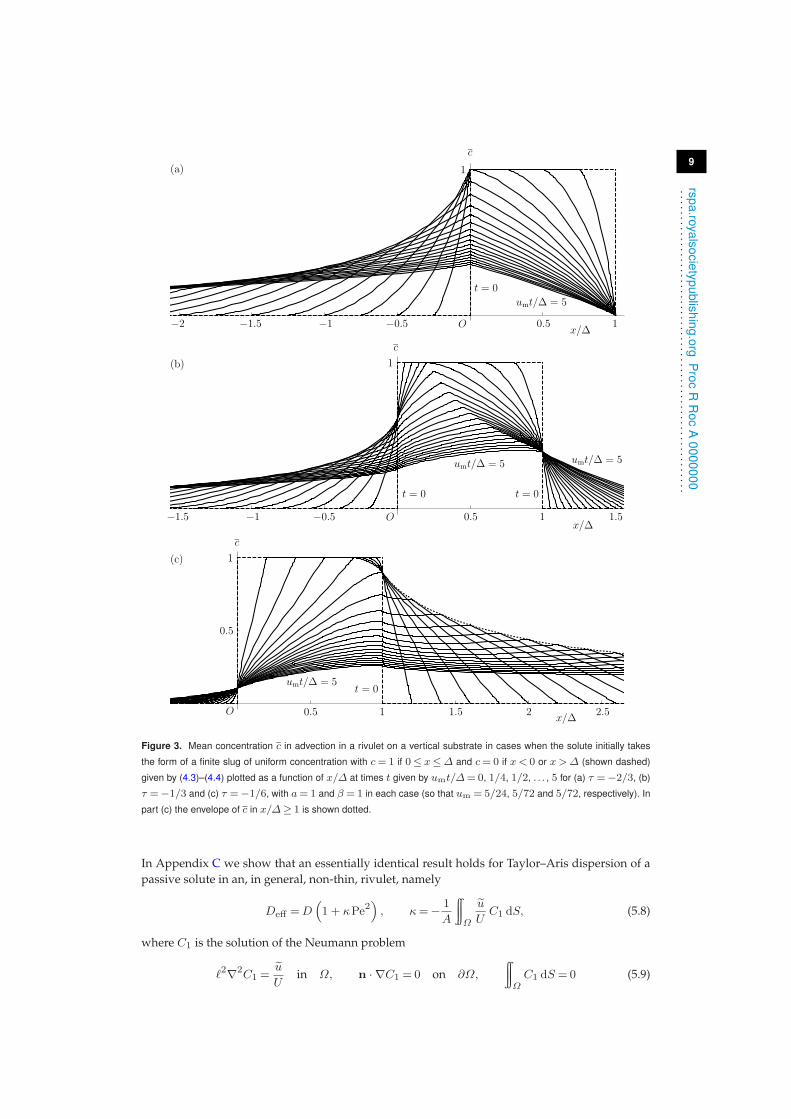
Figure 3 shows three examples of the solution (4.3)–(4.4) for c in a rivulet on a vertical

substrate plotted as a function of x/∆ at several times t, with a= 1 and β = 1, for (a) τ =−2/3

8

rspa.ro

yals

ocie

typublis

hin

g.o

rgP

roc

RR

oc

A0000000

..........................................................

(for which umax = 0, umin =−5/24 and hence um = 5/24), (b) τ =−1/3 (for which umax = 1/72,

umin =−1/18 and hence um = 5/72), and (c) τ =−1/6 (for which umax = 1/18, umin =−1/72

and hence um = 5/72). In particular, in Fig. 3(a) we have τ <−aβ/2 =−1/2, and so all of the

solute is advected upwards, whereas in Fig. 3(b) and (c) we have −1/2 =−aβ/2< τ < 0, and so

both downwards and upwards advection occurs. In Fig. 3(c) (but not in Fig. 3(b)) non-monotonic

dependence of c on x of the kind mentioned earlier is evident in x>∆. All of the solutions shown

in Figure 3 are for cases with τ < 0. Solutions for cases with τ ≥ 0, in which all of the solute is

advected downwards, are somewhat similar to the reflection of Fig. 3(a) in the line x= 1/2, and

so are omitted for brevity.

5. Taylor–Aris dispersion of a passive solute in a rivulet

For times longer than those considered in Section 4, the effects of diffusion are not negligible, and

the concentration c satisfies the general advection–diffusion equation (3.1). In the remainder of the

present work we will be concerned with Taylor–Aris dispersion of the solute at sufficiently long

times. In particular, we will obtain the general expression for the effective diffusivity Deff in the

present rivulet flow. For definiteness we consider a situation somewhat similar to that considered

in Section 4(b), in which the solute initially takes the form of a finite slug in 0≤ x≤∆, where

∆ is a constant, with c= 0 if x< 0 or x>∆, except that now we allow the initial concentration

c(x, y, z, 0) to be nonuniform. We non-dimensionalise and scale variables as in (2.1), together with

x=Lx∗, t=L

Ut∗, c=C0c

∗, Deff =DD∗eff , (5.1)

where L is a characteristic length scale in the x direction and the mean initial concentration C0

now takes the form

C0 =1

A∆

∫∆0

∫a−a

∫h0

c(x, y, z, 0) dz dy dx. (5.2)

Then, with the stars again dropped for clarity, the governing equation and boundary conditions

for c become, without approximation,

δPe(ct + ucx) = δ2cxx +∇2c, n · ∇c= 0 on z = 0 and z = h, (5.3)

where δ= ℓ/L is a longitudinal aspect ratio and Pe is a Péclet number, defined by Pe=Uℓ/D.

The time scale over which Taylor–Aris dispersion of the solute takes place is such that the aspect

ratio δ≪ 1 is small.

As is well known (see, for example, Taylor [4,5], Aris [6] and the references cited in Section 1), in

Taylor–Aris dispersion of a passive solute in, for example, steady unidirectional pressure-driven

flow in a channel of arbitrary cross-section Ω, the problem (5.3) leads to an advection–diffusion

equation for c at leading order in δ, namely, in dimensional terms,

ct + u cx =Deff cxx, (5.4)

where the effective diffusivity Deff is conventionally expressed in the form

Deff =D(1 + κconPe

2con

), κcon =

1

A

∫∫Ω

u

uC1con dS, (5.5)

where Pecon = uL/D (with L denoting a typical diameter ofΩ) is a Péclet number conventionally

used in studies of Taylor–Aris dispersion, A denotes the area of Ω, u= u− u is the varying part

of u which, by definition, satisfies ∫∫Ωu dS = 0, (5.6)

and the dimensionless quantity C1con is the solution of the Neumann problem

L2∇2C1con =− uu

in Ω, n · ∇C1con = 0 on ∂Ω,

∫∫ΩC1con dS = 0. (5.7)

9

rspa.ro

yals

ocie

typublis

hin

g.o

rgP

roc

RR

oc

A0000000

..........................................................

−2 −1.5 −1 −0.5 0.5 1

1(a)

Ox/∆

c

t = 0

umt/∆ = 5

−1.5 −1 −0.5 0.5 1 1.5

1(b)

Ox/∆

c

t = 0 t = 0

umt/∆ = 5 umt/∆ = 5

0.5 1 1.5 2 2.5

0.5

1(c)

Ox/∆

c

t = 0umt/∆ = 5

Figure 3. Mean concentration c in advection in a rivulet on a vertical substrate in cases when the solute initially takes

the form of a finite slug of uniform concentration with c= 1 if 0≤ x≤∆ and c= 0 if x< 0 or x>∆ (shown dashed)

given by (4.3)–(4.4) plotted as a function of x/∆ at times t given by umt/∆= 0, 1/4, 1/2, . . . , 5 for (a) τ =−2/3, (b)

τ =−1/3 and (c) τ =−1/6, with a= 1 and β = 1 in each case (so that um = 5/24, 5/72 and 5/72, respectively). In

part (c) the envelope of c in x/∆≥ 1 is shown dotted.

In Appendix C we show that an essentially identical result holds for Taylor–Aris dispersion of a

passive solute in an, in general, non-thin, rivulet, namely

Deff =D(1 + κPe2

), κ=− 1

A

∫∫Ω

u

UC1 dS, (5.8)

where C1 is the solution of the Neumann problem

ℓ2∇2C1 =u

Uin Ω, n · ∇C1 = 0 on ∂Ω,

∫∫ΩC1 dS = 0 (5.9)

10

rspa.ro

yals

ocie

typublis

hin

g.o

rgP

roc

RR

oc

A0000000

..........................................................

(again written in dimensional terms). We may, of course, choose to regard the quantities κcon,

Pecon and C1con as being related to κ, Pe and C1 by

κcon =

(Uℓ

uL

)2

κ, Pecon =uLUℓ

Pe, C1con =−Uℓ2

uL2C1 (5.10)

(so that κconPe2con = κPe2). However, when we wish to compare values ofDeff in different rivulet

flows with different values of τ , the formulation (5.5)–(5.7) is inconvenient, since both Pecon and

κcon depend on τ (via their dependence on u), whereas in the formulation (5.8)–(5.9) used in the

present study, Pe is independent of τ , and so the dependence ofDeff given by (5.8) on τ is isolated

in just one parameter, namely κ. In addition, when τ takes the critical value τ = τc corresponding

to no net flow, u= 0, not only is the problem (5.7) for C1con singular, but also Pecon is zero and

κcon is infinite (with κconPe2con finite), meaning that in the conventional formulation it would be

necessary to define Deff via a limiting process; the present formulation avoids this complication.

Moreover, if τ < τc then u< 0 and so, slightly confusingly, Pecon is negative; again the present

formulation, in which Pe is always positive, avoids this complication.

We now use the result (5.8)–(5.9) to analyse Taylor–Aris dispersion in a thin rivulet. As might

be expected, the following development is somewhat similar to that of Guell et al. [21] and Ajdari

et al. [24] for pressure-driven flow in a wide channel.2

(a) Taylor–Aris dispersion in a thin rivulet

For a thin rivulet, equation (5.9) gives, with the scalings (2.1) and (5.1),

C1yy +1

ǫ2C1zz = ǫ2(u− u), C1z = 0 on z = 0, C1z = ǫ2C1yh

′ on z = h. (5.11)

If we expand C1 as

C1 = ǫ2(C10 + ǫ2C12 + ǫ4C14 + . . .

), (5.12)

then at leading order in ǫ we obtain

C10zz = 0, C10z = 0 on z = 0, C10z = 0 on z = h, (5.13)

so that C10 =C10(y). At first order in ǫ we obtain

C′′10 + C12zz = u− u, C12z = 0 on z = 0, C12z =C′

10h′ on z = h. (5.14)

Since the contact angle is non-zero, consistency of the boundary conditions in (5.14) at y=±arequires that

C′10 = 0 at y=±a. (5.15)

From (5.14) we have

C12 =sinα

2

(hz3

3− z4

12

)+τz3

6−(u+ C′′

10

) z22

+ k (5.16)

for some arbitrary function k= k(y), with

(hC′

10

)′=R, (5.17)

where for convenience we have written

R=R(y) =sinαh3

3+τh2

2− uh. (5.18)

Therefore

C′10 =

1

h

∫y−a

R(y) dy, (5.19)

2 Note that there is a minor typographical error in equation (7) of Ajdari et al. [24], namely a missing opening square bracket

before the second integral sign.

11

rspa.ro

yals

ocie

typublis

hin

g.o

rgP

roc

RR

oc

A0000000

..........................................................

and hence

C10 =

∫y−a

1

h(y)

∫ y−a

R(y) dy dy, (5.20)

the latter being correct up to an irrelevant additive constant.

Then taking the leading order terms in ǫ in equation (5.8) yields our main result concerning

Taylor–Aris dispersion in a thin rivulet, namely that the general expression for the effective

diffusivity Deff takes the form

Deff = 1 + κ0Pe2, (5.21)

in which Pe=Uℓ/D, and the coefficient κ0 is given by

κ0 =1

A

∫a−a

hC′ 210 dy=

1

A

∫a−a

1

h

(∫y−a

R(y) dy

)2

dy, (5.22)

or, more explicitly, by

κ0 =1

A3

∫a−a

1

h(y)

∫y−a

sinα

3

[I1h(y)

3 − I3h(y)]+τ

2

[I1h(y)

2 − I2h(y)]dy

2

dy. (5.23)

Note that, despite the fact that h(±a) = 0, the integral in (5.23) is convergent.

Since h (given explicitly by (A.1) in Appendix A) depends on α in a non-trivial way, the

dependence of κ0 in (5.23) on α is, in general, rather complicated. On the other hand, for a given

value of α, if a and β are prescribed (in which case h is determined explicitly) then κ0 is simply

quadratic in τ . However, if Q is one of the prescribed quantities, along with either a or β (in

which case h depends on τ via the flux relation (2.7)), then the dependence of κ0 on τ is rather

more complicated. These points may be understood more readily in the special case of a rivulet

on a vertical substrate, which we discuss in detail in Section 5(b) below.

(b) Taylor–Aris dispersion in a thin rivulet on a vertical substrate

In the special case of a rivulet on a vertical substrate, in which h is given by (2.9), equation (5.20)

gives

C10 =hm(a2 − y2

)2 [20hmy

2 − 7a2(8hm + 9τ)]

2520a4, (5.24)

and (5.23) leads to an explicit expression for κ0, namely

κ0 =β2a4

(13388β2a2 + 57876aβτ + 63063τ2

)

331080750, (5.25)

the interpretation of which depends on which two of the three quantities a, β and Q are

prescribed, and on the prescribed value of τ , as we now describe.

(i) Purely gravity-driven flow

In the case τ = 0 equation (5.25) yields κ0 = κGD for dispersion in purely gravity-driven flow,

where

κGD =6694a6β4

165540375≃ 4.0437× 10−5a6β4, (5.26)

which, when written in the form

κGD =3347a2u2

270270≃ 0.0124a2u2, (5.27)

where u= 2a2β2/35, can be recognised as being identical to the result for dispersion in pressure-

driven flow in a wide channel of parabolic cross-section obtained by Ajdari et al. [24]. Since Q=

12

rspa.ro

yals

ocie

typublis

hin

g.o

rgP

roc

RR

oc

A0000000

..........................................................

−3 −2 −1 1

0.01

0.02

0.03

τ

κ0

a = 1

a = 2

a = 3a = 4a = 5

Figure 4. The coefficient κ0 given by (5.25) plotted as a function of τ for a thin rivulet on a vertical substrate driven by

both gravity and a surface shear stress τ , with prescribed a and β. The curves correspond to a= 1 (lowest), 2, 3, 4 and

5 (highest), with β = 1 in each case. (Note that, despite appearances, the curves do not touch the τ axis, that is, κ0 is

strictly positive.)

4a4β3/105 in this case, equation (5.26), which gives the most useful form of κ0 if a and β are

prescribed, may alternatively be written in the equivalent forms

κGD =3347

60060

(Q3

105β

)1/2

≃ 0.0054

(Q3

β

)1/2

, κGD =3347

30030

(aQ2

210

)2/3

≃ 0.0032(aQ2)2/3,

(5.28)

which are more useful if either β and Q are prescribed or a and Q are prescribed, respectively.

(ii) Purely surface-shear-stress-driven flow

In the limit |τ | →∞ equation (5.25) yields κ0, re-scaled as κ0 = τ2κSD, for dispersion in purely

shear-stress-driven flow, namely

κSD =a4β2

5250≃ 0.0002a4β2, (5.29)

or equivalently

κSD =a2u

2

210≃ 0.0048a2u

2, (5.30)

in which u= u/τ → aβ/5. From (2.11), equation (5.29), which gives the most useful form of κ0 if

a and β are prescribed, may alternatively be rewritten in the equivalent forms

κ′SD =1

140

(√3Q2

5√2β

)2/3

≃ 0.0028

(Q2

β

)2/3

, κ′′SD =aQ

700≃ 0.0014aQ, (5.31)

in which κ0 has been re-scaled as κ0 = τ2/3κ′SD and κ0 = τκ′′SD, respectively, and which are more

useful if either β and Q are prescribed or a and Q are prescribed, respectively.

(iii) A rivulet with prescribed a and β

If a and β are prescribed then, as previously mentioned, κ0 in (5.25) is simply quadratic in τ .

Figure 4 shows κ0 given by (5.25) plotted as a function of τ for a range of values of a, with

β = 1; note that whereas a and β are constants on each curve, Q varies along the curves. The

minimum value of κ0 on a given curve is κ0 = 8a4β4/24279255≃ 3.2950× 10−7a4β4, occurring

when τ =−106aβ/231≃−0.4589aβ, and corresponding to Q=−16a4β3/693≃−0.0231a4β3;

13

rspa.ro

yals

ocie

typublis

hin

g.o

rgP

roc

RR

oc

A0000000

..........................................................

for given values of a and β, values of κ0 below this minimum are not achievable for any τ . Note

also that two different values of τ , and hence two rivulets with different fluxes Q (but with the

same values of a and β), can be associated with the same value of κ0; for example, when a= 2

and β = 1, the value κ0 = 0.01 is attained with τ ≃−2.7273 (for which Q≃−2.2996) and with

τ ≃ 0.8918 (for which Q≃ 1.5607).

(iv) A rivulet with prescribed β and Q

If β and Q are prescribed then (2.9), (2.11) and (5.25) give κ0 parametrically as a function of τ

(with parameter a) in the form

τ =15Q

2a3β2− 2aβ

7, κ0 =

8a6β4

1324323+

4Qa2β

8085+

3Q2

280a2β2. (5.32)

In particular, κ0 has branches satisfying

κ0 =1

140

(3Q4τ2

50β2

)1/3

+31

2695

(Q5

60βτ2

)1/3

+O

(1

τ

)→∞ (5.33)

in the limits τ →±∞ (corresponding to a→ 0+), and a branch in τ < 0 satisfying

κ0 =343τ6

30888β2+

38Qτ2

2145β+O(τ)→∞ (5.34)

in the limit τ →−∞ (corresponding to a→+∞). In the special caseQ= 0 (which, for a nontrivial

flow, is possible only for τ < 0), κ0 is simply given by

κ0 =343τ6

30888β2≃ 0.0111

(τ3

β

)2

for τ < 0. (5.35)

Figure 5 shows κ0 given by (5.32) plotted as a function of τ for a range of values of Q, together

with the asymptotic results (5.33)–(5.34), with β = 1 in each case. Note that whereas β and Q are

constants on each curve in Fig. 5, a varies along the curves.

When Q> 0 there is a unique value of κ0 for each value of τ , but when Q satisfies Qmin <

Q< 0, where Qmin =−3087τ4/5120β, there are two values of κ0 for each value of τ < 0. The

latter non-uniqueness arises because, as Wilson and Duffy [33] describe, when τ < 0 there are

two possible values of a (and hence two possible rivulets, a narrower one and a wider one) that

correspond to such a value of Q; these two rivulets are associated with the smaller and larger

values of κ0, respectively. As Wilson and Duffy [33] also show, there is no rivulet solution when

Q satisfies Q<Qmin, or equivalently, when τ > τmax, where τmax =−(−5120βQ/3087)1/4 for

Q< 0; this is consistent with the fact that the curves for Q< 0 in Fig. 5 lie entirely in τ ≤ τmax.

As Fig. 5 shows, κ0 again has a minimum as a function of τ , namely

κ0 =1

1155

(2(11518 + 217

√2821σ

)Q3

1365β

)1/2

≃ 0.0050

(Q3

β

)1/2

or 0.0001

(−Q

3

β

)1/2

,

(5.36)

when

τ = σ

(2(32874353

√2821σ − 1662451778

)βQ

3471933465

)1/4

≃ 0.4685 (βQ)1/4 or −1.1837 (−βQ)1/4 ,

(5.37)

corresponding to

a=

(21(√

2821σ − 26)Q

40β3

)1/4

≃ 1.9424

(Q

β3

)1/4

or 2.5386

(− Q

β3

)1/4

, (5.38)

where we have written σ= sgn(Q) =±1, and the decimal approximations are valid for Q> 0

and Q< 0, respectively. For given values of β and Q, values of κ0 below this minimum are not

14

rspa.ro

yals

ocie

typublis

hin

g.o

rgP

roc

RR

oc

A0000000

..........................................................

−4 −2 2 4

0.01

0.02

0.03

τ

κ0

Q = −3

Q = −2

Q = −1

Q = 0

Q = 1

Q = 2

Q = 3

Figure 5. The coefficient κ0 given by (5.32) plotted as a function of τ for a thin rivulet on a vertical substrate driven by

both gravity and a surface shear stress τ , with prescribed β and Q. The curves correspond to Q=−3, −2, −1, . . . , 3,

with β = 1 in each case. The dashed and dotted curves show the asymptotic results (5.33)–(5.34), respectively.

achievable for any τ ; moreover, except when Q= 0, any value of κ0 above its minimum can be

achieved with two different values of τ , and hence with two different rivulets.

(v) A rivulet with prescribed a and Q

If a and Q are prescribed then κ0 is again given parametrically as a function of τ by (5.32), but is

now parameterised by β (rather than by a). Qualitatively the behaviour in this case is somewhat

similar to that in the case of prescribed β and Q described in Section 5(b)(iv). In particular, κ0 has

branches satisfying

κ0 =aQτ

700+

73

5390

(aQ3

30τ

)1/2

+O

(1

τ

)→∞ (5.39)

in the limits τ →±∞ (corresponding to β→ 0+), and a branch in τ < 0 satisfying

κ0 =7a2τ4

7722− 178aQτ

45045+O(1)→∞ (5.40)

in the limit τ →−∞ (corresponding to β→+∞). In the special case Q= 0, κ0 is simply given by

κ0 =7a2τ4

7722≃ 0.0009

(aτ2)2

for τ < 0. (5.41)

Figure 6 shows κ0 given by (5.32) plotted as a function of τ for a range of values of Q, together

with the asymptotic results (5.39)–(5.40), with a= 1 in each case. Note that whereas a and Q are

constants on each curve in Fig. 6, β varies along the curves.

As in the case of prescribed β andQ described in Section 5(b)(iv), whenQ> 0 there is a unique

value of κ0 for each value of τ , but whenQ satisfiesQmin <Q< 0, where nowQmin = 98τ3a/405,

15

rspa.ro

yals

ocie

typublis

hin

g.o

rgP

roc

RR

oc

A0000000

..........................................................−4 −2 2 4

0.01

0.02

0.03

τ

κ0

Q = −3

Q = −2

Q = −1

Q = 0

Q = 1

Q = 2

Q = 3

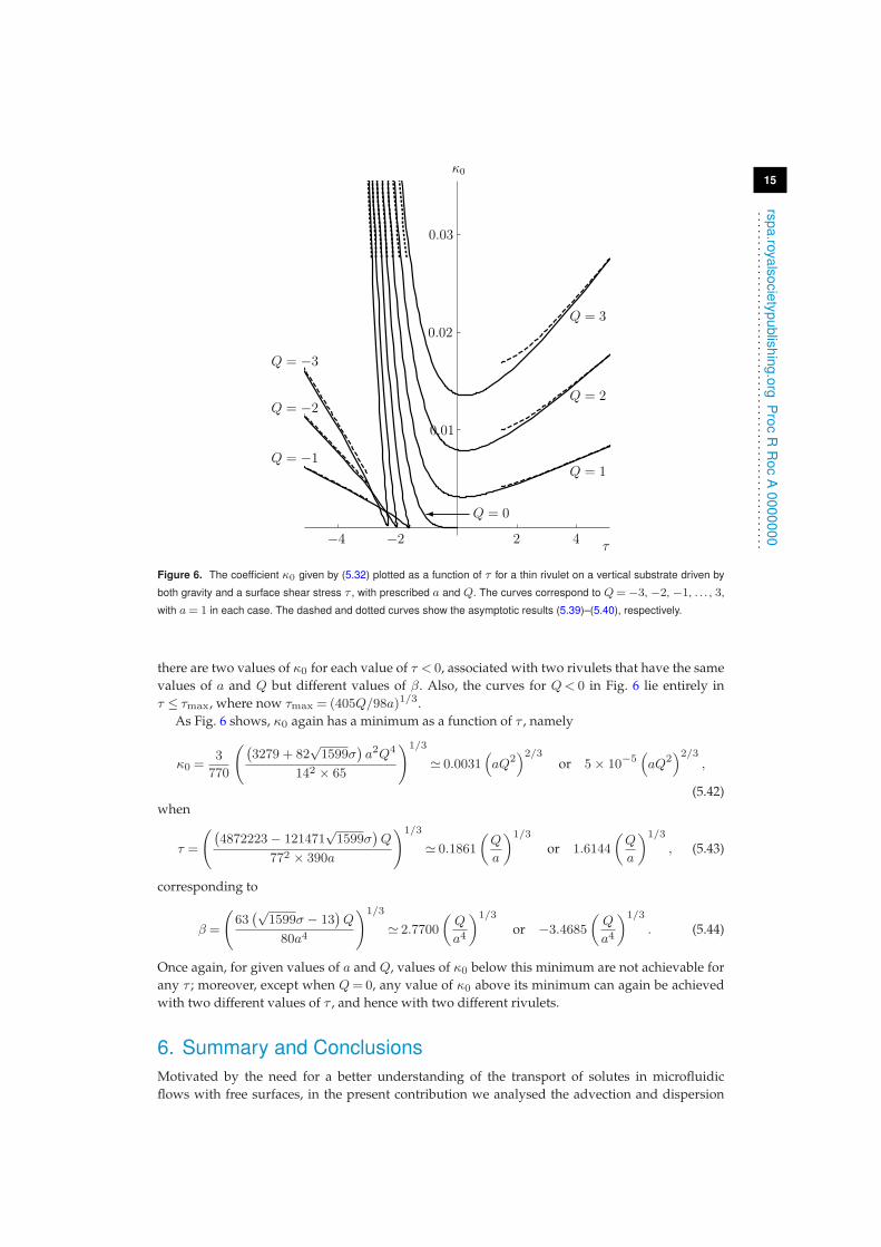
Figure 6. The coefficient κ0 given by (5.32) plotted as a function of τ for a thin rivulet on a vertical substrate driven by

both gravity and a surface shear stress τ , with prescribed a and Q. The curves correspond to Q=−3, −2, −1, . . . , 3,

with a= 1 in each case. The dashed and dotted curves show the asymptotic results (5.39)–(5.40), respectively.

there are two values of κ0 for each value of τ < 0, associated with two rivulets that have the same

values of a and Q but different values of β. Also, the curves for Q< 0 in Fig. 6 lie entirely in

τ ≤ τmax, where now τmax = (405Q/98a)1/3.

As Fig. 6 shows, κ0 again has a minimum as a function of τ , namely

κ0 =3

770

((3279 + 82

√1599σ

)a2Q4

142 × 65

)1/3

≃ 0.0031(aQ2

)2/3or 5× 10−5

(aQ2

)2/3,

(5.42)

when

τ =

((4872223− 121471

√1599σ

)Q

772 × 390a

)1/3

≃ 0.1861

(Q

a

)1/3

or 1.6144

(Q

a

)1/3

, (5.43)

corresponding to

β =

(63(√

1599σ − 13)Q

80a4

)1/3

≃ 2.7700

(Q

a4

)1/3

or −3.4685

(Q

a4

)1/3

. (5.44)

Once again, for given values of a and Q, values of κ0 below this minimum are not achievable for

any τ ; moreover, except when Q= 0, any value of κ0 above its minimum can again be achieved

with two different values of τ , and hence with two different rivulets.

6. Summary and Conclusions

Motivated by the need for a better understanding of the transport of solutes in microfluidic

flows with free surfaces, in the present contribution we analysed the advection and dispersion

16

rspa.ro

yals

ocie

typublis

hin

g.o

rgP

roc

RR

oc

A0000000

..........................................................

of a passive solute in steady unidirectional flow of a thin uniform rivulet on an inclined planar

substrate driven by gravity and/or a uniform longitudinal surface shear stress.

In Section 4 we described the short-time advection of both an initially semi-infinite and an

initally finite slug of solute of uniform concentration. Examples were presented showing both

downwards and upwards advection of solute, highlighting the fact that the dependence of c on x

is not, in general, piecewise linear, and can develop additional non-monotonic dependence on x

beyond what it inherits in an obvious way from the initial distribution of c.

In Section 5 we described the long-time Taylor–Aris dispersion of an initially finite slug of

solute. In Appendix C we used the method of multiple scales to derive the formal expression

for the effective diffusivity Deff of a non-thin rivulet (or indeed any channel of arbitrary cross-

section), from which in Section 5(a) we obtained our main result, namely the general expression

for Deff in a thin rivulet given by equations (5.21)–(5.23). In doing so, particular care was taken to

formulate the problem in such a way as to avoid the complications that arise when u≤ 0 (i.e. when

Q≤ 0) when using the conventional formulation of the problem. In Section 5(b) we obtained the

explicit expression forDeff in the special case of a rivulet on a vertical substrate given by equations

(5.21) and (5.25), and discussed in detail its different interpretations depending on which two of

the three quantities a, β and Q are prescribed. In all three situations considered we found that,

except in the special case of no net flow, Q= 0, the coefficient κ0 always has a strictly positive

global minimum as a function of τ (i.e. that Deff is always strictly greater than D) and that any

value of κ0 above its minimum value can be achieved with two different values of τ (i.e. with two

different rivulets).

As noted in Section 1, while the present work was primarily motivated by and described in

the context of the dispersion of a solute, the present results also apply to the transport of heat

with insulating boundary conditions and can readily be extended to other thermal boundary

conditions, and so the present work is also relevant to the wide range of practical situations

involving heat transfer in the presence of rivulets.

Data Accessibility. There are no datasets associated with the present work.

Competing Interests. We have no competing interests.

Authors’ Contributions. B.R.D. and S.K.W. conceived of the study and drafted the manuscript. All three

authors contributed to the mathematical calculations described in the present work and gave final approval

for publication.

Funding. The first author (F.H.H.A.) was supported financially by the Ministry of Higher Education,

Kingdom of Saudi Arabia and King Faisal University via an Academic Staff Training Fellowship. The

third author (S.K.W.) was partially supported financially by the Leverhulme Trust via Research Fellowship

RF-2013-355.

References

1. Stone HA, Stroock AD, Ajdari A. 2004 Engineering flows in small devices:Microfluidics toward a lab-on-a-chip, Annu. Rev. Fluid Mech. 36, 381–411. (doi:10.1146/annurev.fluid.36.050802.122124)

2. Darhuber AA, Troian SM. 2005 Principles of microfluidic actuation by modulation of surfacestresses, Annu. Rev. Fluid Mech. 37, 425–455. (doi: 10.1146/annurev.fluid.36.050802.122052)

3. Lee C-Y, Chang C-L, Wang Y-N, Fu L-M. 2011 Microfluidic mixing: A review, Int. J. Mol. Sci.12, 3263–3287. (doi: 10.3390/ijms12053263)

4. Taylor GI. 1953 Dispersion of soluble matter in solvent flowing slowly through a tube. Proc.Roy. Soc. Lond. A 219, 186–203. (doi: 10.1098/rspa.1953.0139)

5. Taylor GI. 1954 Conditions under which dispersion of a solute in a stream of solventcan be used to measure molecular diffusion. Proc. Roy. Soc. Lond. A 225, 473–477. (doi:10.1098/rspa.1954.0216)

6. Aris R. 1956 On the dispersion of a solute in a fluid flowing through a tube. Proc. Roy. Soc.Lond. A 235, 67–77. (doi: 10.1098/rspa.1956.0065)

7. Witelski T, Bowen M. 2015 Methods of Mathematical Modelling. New York: Springer.

17

rspa.ro

yals

ocie

typublis

hin

g.o

rgP

roc

RR

oc

A0000000

..........................................................

8. Lungu EM, Moffatt HK. 1982 The effect of wall conductance on heat diffusion in duct flow. J.Eng. Math. 16, 121–136. (doi: 10.1007/BF00042550)

9. Pagitsas M, Nadim A, Brenner H. 1986 Multiple time scale analysis of macrotransportprocesses. Physica A 135, 533–550. (doi: 10.1016/0378-4371(86)90158-5)

10. Zhang J, Frigaard IA. 2006 Dispersion effects in the miscible displacement of two fluids in aduct of large aspect ratio. J. Fluid Mech. 549, 225–251. (doi: 10.1017/S0022112005007846)

11. Mercer GN, Roberts AJ. 1990 A centre manifold description of contaminant dispersionin channels with varying flow properties. SIAM J. Appl. Math. 50, 1547–1565. (doi:10.1137/0150091)

12. Young WR, Jones S. 1991 Shear dispersion. Phys. Fluids A 3, 1087–1101. (doi: 10.1063/1.858090)13. Balakotaiah V, Chang H-C. 1995 Dispersion of chemical solutes in chromatographs and

reactors. Phil. Trans. Roy. Soc. Lond. A 351, 39–75. (doi: 10.1098/rsta.1995.0025)14. Ratnakar RR, Balakotaiah V. 2011 Exact averaging of laminar dispersion. Phys. Fluids 23,

023601. (doi: 10.1063/1.3555156)15. Brenner H, Edwards DA. 1993 Macrotransport Processes. Oxford: Butterworth–Heinemann.16. Dutta D, Leighton Jr DT. 2001 Dispersion reduction in pressure-driven flow through

microetched channels. Anal. Chem. 73, 504–513. (doi: 10.1021/ac0008385)17. Dutta D, Ramachandran A, Leighton Jr, DT. 2006 Effect of channel geometry on solute

dispersion in pressure-driven microfluidic systems. Microfluid Nanofluid 2, 275–290. (doi:10.1007/s10404-005-0070-7)

18. Dutta D. 2015 Hydrodynamic dispersion. In Encyclopedia of Microfluidics and Nanofluidics(edited by D. Li), pp 1313–1325. New York: Springer.

19. Doshi MR, Daiya PM, Gill WN. 1978 Three dimensional laminar dispersion in open and closedrectangular conduits. Chem. Eng. Sci. 33, 795–804. (doi: 10.1016/0009-2509(78)85168-9)

20. Chatwin PC, Sullivan PJ. 1982 The effect of aspect ratio on longitudinal diffusivity inrectangular channels. J. Fluid Mech. 120, 347–358. (doi: 10.1017/S0022112082002791)

21. Guell DC, Cox RG, Brenner H. 1987 Taylor dispersion in conduits of large aspect ratio. Chem.Eng. Comm. 58, 231–244. (doi: 10.1080/00986448708911970)

22. Smith R. 1990 Two-dimensional shear dispersion for skewed flows in narrow gaps betweenmoving surfaces. J. Fluid Mech. 214, 211–228. (doi: 10.1017/S0022112090000118)

23. Smith R. 1990 Shear dispersion along a rotating axle in a closely fitting shaft. J. Fluid Mech.219, 647–658. (doi: 10.1017/S0022112090003135)

24. Ajdari A, Bontoux N, Stone HA. 2006 Hydrodynamic dispersion in shallow microchannels:the effect of cross-sectional shape. Anal. Chem. 78, 387–392. (doi: 10.1021/ac0508651)

25. Darhuber AA, Chen JZ, Davis JM, Troian SM. 2004 A study of mixing in thermocapillaryflows on micropatterned surfaces. Phil. Trans. Roy. Soc. Lond. A 362, 1037–1058. (doi:10.1098/rsta.2003.1361)

26. Kabov OA. 2010 Interfacial thermal fluid phenomena in thin liquid films. Int. J. EmergingMultidisciplinary Fluid Sci. 2, 87–121. (doi: 10.1260/1756-8315.2.2-3.87)

27. Kabov OA, Bartashevich MV, Cheverda V. 2010 Rivulet flows in microchannels andminichannels. Int. J. Emerging Multidisciplinary Fluid Sci. 2, 161–182. (doi: 10.1260/1756-8315.2.2-3.161)

28. Paterson C, Wilson SK, Duffy BR. 2013 Pinning, de-pinning and re-pinning of a slowly varyingrivulet. Euro. J. Mech. B/Fluids 41, 94–108. (doi: 10.1016/j.euromechflu.2013.02.006)

29. Young GW, Davis SH. 1987 Rivulet instabilities. J. Fluid Mech. 176, 1–31. (doi:10.1017/S0022112087000557)

30. Duffy BR, Moffatt HK. 1995 Flow of a viscous trickle on a slowly varying incline. Chem. Eng.J. 60, 141–146. (doi: 10.1016/0923-0467(95)03030-1)

31. Myers TG, Liang HX, Wetton B. 2004 The stability and flow of a rivulet drivenby interfacial shear and gravity. Int. J. Non-Linear Mech. 39, 1239–1249. (doi:10.1016/j.ijnonlinmec.2003.08.001)

32. Saber HH, El-Genk MS. 2004 On the breakup of a thin liquid film subject to interfacial shear.J. Fluid Mech. 500, 113–133. (doi: 10.1017/S0022112003007080)

33. Wilson SK, Duffy BR. 2005 Unidirectional flow of a thin rivulet on a vertical substratesubject to a prescribed uniform shear stress at its free surface. Phys. Fluids 17, 108105. (doi:10.1063/1.2100987)

34. Sullivan JM, Wilson SK, Duffy BR. 2008 A thin rivulet of perfectly wetting fluidsubject to a longitudinal surface shear stress. Q. J. Mech. Appl. Math. 61, 25–61. (doi:10.1093/qjmam/hbm023)

18

rspa.ro

yals

ocie

typublis

hin

g.o

rgP

roc

RR

oc

A0000000

..........................................................

35. Benilov ES. 2009 On the stability of shallow rivulets. J. Fluid Mech. 636, 455–474. (doi:10.1017/S0022112009990802)

36. Tanasijczuk AJ, Perazzo CA, Gratton J. 2010 Navier–Stokes solutions for steady parallel-sidedpendent rivulets. Eur. J. Mech. B/Fluids 29, 465–471. (doi: 10.1016/j.euromechflu.2010.06.002)

37. Wilson SK, Sullivan JM, Duffy BR. 2011 The energetics of the breakup of a sheet and of arivulet on a vertical substrate in the presence of a uniform surface shear stress. J. Fluid Mech.674, 281–306. (doi: 10.1017/S0022112010006518)

38. Herrada MA, Mohamed AS, Montanero JM, Gañán-Calvo AM. 2015 Stabilityof a rivulet flowing in a microchannel. Int. J. Multiphase Flow 69, 1–7. (doi:10.1016/j.ijmultiphaseflow.2014.10.012)

39. Bender CM, Orszag, SA. 1999 Advanced Mathematical Methods for Scientists and Engineers I:Asymptotic Methods and Perturbation Theory. New York: Springer.

A. The solution of equations (2.5)–(2.6) for hIn this Appendix we record the solution of (2.5)–(2.6) for the profile h(y) of a thin uniform rivulet

undergoing steady unidirectional flow on a planar substrate inclined at an angle α (0≤ α≤ π)

to the horizontal, the flow being driven by gravity and/or a uniform longitudinal surface shear

stress τ . We also provide explicit expressions for the quantities I1, I2 and I3 defined in (2.8) and

appearing in the expressions for Q and u given in (2.7).

The solution of (2.5) subject to (2.6) is

h= β ×

coshma− coshmy

m sinhmaif 0≤ α<

π

2,

a2 − y2

2aif α=

π

2,

cosmy − cosma

m sinmaif

π

2<α≤ π,

(A.1)

where we have introduced the notation m= | cosα|. Therefore the maximum thickness of the

rivulet, hm = h(0), is given by

hm =β

m×

tanhma

2if 0≤ α<

π

2,

ma

2if α=

π

2,

tanma

2if

π

2<α≤ π,

(A.2)

and the flux Q and mean velocity u are given by (2.7), in which the In defined in (2.8) are given

by

I1 =2β

m2×

ma cothma− 1 if 0≤ α<π

2,

(ma)2

3if α=

π

2,

1−ma cotma ifπ

2<α≤ π,

(A.3)

I2 =β2

m3×

3ma coth2ma− 3 cothma−ma if 0≤ α<π

2,

4(ma)3

15if α=

π

2,

3ma cot3ma− 3 cotma+ma ifπ

2<α≤ π,

(A.4)

19

rspa.ro

yals

ocie

typublis

hin

g.o

rgP

roc

RR

oc

A0000000

..........................................................

I3 =β3

3m4×

15ma coth3ma− 15 coth2ma− 9ma cothma+ 4 if 0≤ α<π

2,

12(ma)4

35if α=

π

2,

−15ma cot3ma+ 15 cot2ma− 9ma cotma+ 4 ifπ

2<α≤ π.

(A.5)

In all of the above, if 0≤ α≤ π/2 then ma≥ 0, whereas if π/2<α≤ π then 0<ma≤ π. Note that

the expressions for I2 and I3 were first given in these compact forms by Sullivan et al. [34] and

Duffy and Moffatt [30], respectively.

B. Advection in a rivulet: two cases in which u≥ 0 everywhere

In this Appendix we obtain explicit expressions for the function f appearing in equations (4.2),

(4.3)–(4.4) in two cases in which u≥ 0 everywhere, namely flow on a vertical substrate with τ ≥ 0

and purely surface-shear-stress-driven flow.

(a) Flow on a vertical substrate with τ ≥ 0

In the case of flow on a vertical substrate (i.e. whenα= π/2) and τ ≥ 0, in which case um = umax =

hm(hm + 2τ)/2 and umin = 0, the condition u≥ x/t for any value of x satisfying 0≤ x≤ umaxt

is equivalent to the condition H ≤ z ≤ h, where z =H (0≤H ≤ h) denotes the curve on which

u= x/t, so that from (2.4)

H = h+ τ −[(h+ τ)2 − 2x

t

]1/2. (B.1)

The curve (B.1) intersects the free surface z = h at y=±b, where

b= a

[1 +

τ

hm−(τ2

h2m+

2x

h2mt

)1/2]1/2

, (B.2)

and the function f in (4.2) is given by

f =

∫b−b

∫hH

dz dy=

∫b−b

(h−H) dy, (B.3)

which leads to

f =

[1 +

τ

hm+

(2x

h2mt

)1/2]1/2 [(

1 +τ

hm

)E(φ|m)−

(2x

h2mt

)1/2

F (φ|m)

]

− τ

hm

[1 +

τ

hm−(τ2

h2m+

2x

h2mt

)1/2]1/2

,

(B.4)

where F and E denote incomplete elliptic integrals of the first and second kinds, respectively,

with

φ= sin−1

1 +τ

hm−(τ2

h2m+

2x

h2mt

)1/2

1 +τ

hm−(

2x

h2mt

)1/2

1/2, m=

1 +τ

hm−(

2x

h2mt

)1/2

1 +τ

hm+

(2x

h2mt

)1/2. (B.5)

In particular, in the case of purely gravity-driven flow (τ = 0) equations (B.4)–(B.5) reduce to

f =

[1 +

(2x

h2mt

)1/2]1/2 [

E(m)−(

2x

h2mt

)1/2

K(m)

], m=

1−(

2x

h2mt

)1/2

1 +

(2x

h2mt

)1/2, (B.6)

20

rspa.ro

yals

ocie

typublis

hin

g.o

rgP

roc

RR

oc

A0000000

..........................................................

whereK andE denote complete elliptic integrals of the first and second kinds, respectively. From

(B.4) we have∂f

∂x=− 3F (φ|m)

2h2mt

[1 +

τ

hm+

(2x

h2mt

)1/2]1/2 , (B.7)

showing that ∂f/∂x< 0 for 0≤ x≤ umaxt, that is, f decreases monotonically with x. In Fig. 2 the

curves for τ ≥ 1/6 and the curve for τ = 0 correspond to (B.4) and (B.6), respectively.

(b) Purely surface-shear-stress-driven flow

In the case of purely shear-stress-driven flow, for which u= τz, um = umax = τhm and umin = 0,

a similar analysis to that outlined in Section B(a) reveals that the corresponding forms for H and

b are H = x/τt and

b=

1

mcosh−1

(coshma− (coshma− 1)x

τhmt

)if 0≤ α<

π

2,

a

(1− x

τhmt

)1/2

if α=π

2,

1

mcos−1

(cosma+

(1− cosma)x

τhmt

)if

π

2<α≤ π,

(B.8)

where m is again defined by m= | cosα|. Then from (3.4) the function f in (4.2) is given by

f =

1

ma coshma− sinhma

(mb coshma− sinhmb− (coshma− 1)

mbx

τhmt

)if 0≤ α<

π

2,

(1− x

τhmt

)3/2

if α=π

2,

1

ma cosma− sinma

(mb cosma− sinmb+ (1− cosma)

mbx

τhmt

)if

π

2<α≤ π

(B.9)

for 0≤ x≤ τhmt. From (B.9) we have

∂f

∂x=− 1

τhmt

mb(coshma− 1)

ma coshma− sinhmaif 0≤ α<

π

2,

3

2

(1− x

τhmt

)1/2

if α=π

2,

mb(1− cosma)

sinma−ma cosmaif

π

2<α≤ π,

(B.10)

showing again that ∂f/∂x< 0 for 0≤ x≤ umaxt, that is, f decreases monotonically with x.

C. Taylor–Aris dispersion in a non-thin rivulet

In this Appendix we use the method of multiple scales to derive from (5.3) the formal expression

for the effective diffusivity Deff of an, in general, non-thin rivulet, from which in Section 5 we will

obtain our main result, namely the general expression forDeff in a thin rivulet given by equations

(5.21)–(5.23). In fact, the following analysis is valid not only for rivulet flow but for Taylor–Aris

dispersion in steady unidirectional flow along any channel of arbitrary cross-section.

The time scale over which Taylor–Aris dispersion takes place is such that the aspect ratio δ≪ 1

is small, and we seek the leading order behaviour of Deff in the limit δ→ 0 with Pe=O(1).

First, it is convenient to change to a frame moving with velocity u; writing ξ = x− u t and

T = t we have

δPe(cT + u cξ) = δ2cξξ +∇2c, n · ∇c= 0 on z = 0 and z = h, (C.1)

where u= u− u.

21

rspa.ro

yals

ocie

typublis

hin

g.o

rgP

roc

RR

oc

A0000000

..........................................................

We use a multiple-scales expansion (see, for example, Bender and Orszag [39]), with times Tn(n= 0, 1, 2, . . . ) defined by Tn = δnT , so that (C.1) gives

δPe(cT0

+ δcT1+ δ2cT2

+ u cξ

)= δ2cξξ +∇2c+O(δ3). (C.2)

We expand c as c= c0 + δc1 + δ2c2 +O(δ3) with cn = cn(ξ, y, z, T0, T1, . . . ); then (C.2) leads to

∇2c0 = 0, (C.3)

Pe(c0T0

+ u c0ξ)=∇2c1, (C.4)

Pe(c1T0

+ c0T1+ u c1ξ

)= c0ξξ +∇2c2, (C.5)

and so on. Also the boundary condition in (C.1) gives

n · ∇cn = 0 on z = 0 and z = h, n= 0, 1, 2, . . . . (C.6)

Multiplying (C.3) by c0, integrating over the cross-section of the rivulet, Ω, and using Green’s

theorem and (C.6) yields

0 =

∫∫Ωc0∇2c0 dS

=

∫∫Ω

[∇ · (c0∇c0)− (∇c0 · ∇c0)

]dS

=

∮∂Ω

c0∇c0 · n ds−∫∫Ω

∣∣∇c0∣∣2 dS

=−∫∫Ω

∣∣∇c0∣∣2 dS, (C.7)

where ∂Ω denotes the boundary of Ω (comprising the substrate z = 0 and the free surface z = h)

and s denotes arc length along ∂Ω. Therefore∣∣∇c0

∣∣2 = 0, and so c0y = c0z = 0, showing that c0 is

independent of y and z.

Integration of (C.4) over Ω gives ∫∫Ω∇2c1 dS =APe c0T0

. (C.8)

Using Green’s theorem and (C.6) with n= 1 we have∫∫Ω∇2c1 dS =

∮∂Ω

∇c1 · n ds= 0, (C.9)

so that (C.8) gives c0T0= 0. We deduce that c0 depends on ξ, T1, T2, . . . only, and, from (C.4), that

c1 therefore satisfies

∇2c1 =Pe u c0ξ. (C.10)

Defining C1 =C1(ξ, y, z, T0, T1, . . . ) by

c1 =Pe c0ξC1, (C.11)

C1 satisfies the Neumann problem

∇2C1 = u in Ω, n · ∇C1 = 0 on ∂Ω. (C.12)

Clearly C1 is determined only up to an additive function of ξ, T0, T1, . . . , that is, if C1 = φ1(y, z)

is one solution of (C.12) then so is C1 = φ1(y, z) + ψ1(ξ, T0, T1, . . . ), with ψ1 arbitrary. It is

convenient to choose ψ1 to be minus the cross-sectional mean of φ1 (which is a constant,

independent of ξ, y, z, T0, T1, . . . ); then C1 depends on y and z only, and∫∫ΩC1 dS = 0, (C.13)

with which (C.12) determines C1 uniquely.

22

rspa.ro

yals

ocie

typublis

hin

g.o

rgP

roc

RR

oc

A0000000

..........................................................

Integration of (C.5) over Ω gives

Pe

(∫∫Ωc1T0

dS +Ac0T1+

∫∫Ωu c1ξ dS

)=Ac0ξξ +

∫∫Ω∇2c2 dS, (C.14)

which, using Green’s theorem and (C.11), may be written in the form

Pe

[Pe c0ξ

∂

∂T0

∫∫ΩC1 dS +Ac0T1

+ Pe∂

∂ξ

(c0ξ

∫∫Ωu C1 dS

)]=Ac0ξξ +

∮∂Ω

∇c2 · n ds.

(C.15)

Using (C.6) and (C.13) then gives

PeAc0T1+ Pe2c0ξξ

∫∫Ωu C1 dS =Ac0ξξ, (C.16)

leading to the formal expression for the effective diffusivity Deff , namely

c0T1=Deff

Pec0ξξ, Deff = 1 + κPe2, κ=− 1

A

∫∫Ωu C1 dS, (C.17)

where C1 is the solution of (C.12)–(C.13).

Moreover, using Green’s theorem and (C.12) we have∫∫Ωu C1 dS =

∫∫ΩC1∇2C1 dS

=

∫∫Ω

[∇ · (C1∇C1)− (∇C1 · ∇C1)

]dS

=

∮∂Ω

C1∇C1 · n ds−∫∫Ω

∣∣∇C1

∣∣2 dS

=−∫∫Ω

∣∣∇C1

∣∣2 dS, (C.18)

so that Deff in (C.17) may be written in the alternative form

Deff = 1 + κPe2, κ=1

A

∫∫Ω

∣∣∇C1

∣∣2 dS, (C.19)

which shows, in particular, that Deff > 1.

In dimensional terms the formal expression (C.17) is

c0t + uc0x =Deff c0xx, Deff =D(1 + κPe2

), κ=− 1

A

∫∫Ω

u

UC1 dS, Pe=

Uℓ

D,

(C.20)

showing that at leading order in δ the solute moves with the mean velocity u and diffuses with

an effective diffusivityDeff . Note also that c= c0 at leading order in δ, and so the first equation in

(C.20) may alternatively be written in the form ct + u cx =Deff cxx, which is equation (5.4).