Advanc Database
145
Advance Data Base 1819 1 UNIT-1 A database is an organized collection of data. The data are typically organized to model relevant aspects of reality in a way that supports processes requiring this information. For example, modelling the availability of rooms in hotels in a way that supports finding a hotel with vacancies. Database management systems (DBMSs) are specially designed software applications that interact with the user, other applications, and the database itself to capture and analyze data. A general-purpose DBMS is a software system designed to allow the definition, creation, querying, update, and administration of databases. Well-known DBMSs include MySQL, MariaDB, PostgreSQL, SQLite, Microsoft SQL Server, Microsoft Access, Oracle, SAP HANA, dBASE, FoxPro, IBM DB2, LibreOffice Base, FileMaker Pro and InterSystems Caché. A database is not generally portable across different DBMSs, but different DBMSs can interoperate by using standards such as SQL and ODBC or JDBC to allow a single application to work with more than one database. The interactions catered for by most existing DBMSs fall into four main groups: Data definition – Defining new data structures for a database, removing data structures from the database, modifying the structure of existing data. Update – Inserting, modifying, and deleting data. Retrieval – Obtaining information either for end-user queries and reports or for processing by applications. Administration – Registering and monitoring users, enforcing data security, monitoring performance, maintaining data integrity, dealing with concurrency control, and recovering information if the system fails. A DBMS is responsible for maintaining the integrity and security of stored data, and for recovering information if the system fails. Purpose of Database Systems: 1. To see why database management systems are necessary, let's look at a typical ``file- processing system'' supported by a conventional operating system. The application is a savings bank: o Savings account and customer records are kept in permanent system files. o Application programs are written to manipulate files to perform the following tasks: Debit or credit an account.
-
Upload
nazimahmed -
Category
Documents
-
view
28 -
download
5
description
Advanc DatabaseJNTU H Mtech
Transcript of Advanc Database
Advance Data Base 1819
1
UNIT-1
A database is an organized collection of data. The data are typically organized to model
relevant aspects of reality in a way that supports processes requiring this information. For
example, modelling the availability of rooms in hotels in a way that supports finding a hotel
with vacancies.
Database management systems (DBMSs) are specially designed software applications
that interact with the user, other applications, and the database itself to capture and
analyze data. A general-purpose DBMS is a software system designed to allow the
definition, creation, querying, update, and administration of databases. Well-known DBMSs
include MySQL, MariaDB, PostgreSQL, SQLite, Microsoft SQL Server, Microsoft Access,
Oracle, SAP HANA, dBASE, FoxPro, IBM DB2, LibreOffice Base, FileMaker Pro and
InterSystems Caché. A database is not generally portable across different DBMSs, but
different DBMSs can interoperate by using standards such as SQL and ODBC or JDBC to
allow a single application to work with more than one database.
The interactions catered for by most existing DBMSs fall into four main groups:
Data definition – Defining new data structures for a database, removing data structures from the database, modifying the structure of existing data.
Update – Inserting, modifying, and deleting data. Retrieval – Obtaining information either for end-user queries and reports or for
processing by applications. Administration – Registering and monitoring users, enforcing data security,
monitoring performance, maintaining data integrity, dealing with concurrency control, and recovering information if the system fails.
A DBMS is responsible for maintaining the integrity and security of stored data, and for recovering information if the system fails.
Purpose of Database Systems:
1. To see why database management systems are necessary, let's look at a typical ``file-
processing system'' supported by a conventional operating system.
The application is a savings bank:
o Savings account and customer records are kept in permanent system files.
o Application programs are written to manipulate files to perform the
following tasks:
Debit or credit an account.
Advance Data Base 1819
2
Add a new account.
Find an account balance.
Generate monthly statements.
2. Development of the system proceeds as follows:
o New application programs must be written as the need arises.
o New permanent files are created as required.
o but over a long period of time files may be in different formats, and
o Application programs may be in different languages.
3. So we can see there are problems with the straight file-processing approach:
o Data redundancy and inconsistency
Same information may be duplicated in several places.
All copies may not be updated properly.
o Difficulty in accessing data
May have to write a new application program to satisfy an unusual
request.
E.g. find all customers with the same postal code.
Could generate this data manually, but a long job...
o Data isolation
Data in different files.
Data in different formats.
Difficult to write new application programs.
o Multiple users
Want concurrency for faster response time.
Need protection for concurrent updates.
E.g. two customers withdrawing funds from the same account at the
same time - account has $500 in it, and they withdraw $100 and $50.
The result could be $350, $400 or $450 if no protection.
o Security problems
Every user of the system should be able to access only the data they
are permitted to see.
E.g. payroll people only handle employee records, and cannot see
customer accounts; tellers only access account data and cannot see
payroll data.
Difficult to enforce this with application programs.
o Integrity problems
Data may be required to satisfy constraints.
E.g. no account balance below $25.00.
Again, difficult to enforce or to change constraints with the file-
processing approach.
Advance Data Base 1819
3
These problems and others led to the development of database management
systems.
Data Abstraction:-
The major purpose of a database system is to provide users with an abstract view of the system.
The system hides certain details of how data is stored and created and maintained
Complexity should be hidden from database users.
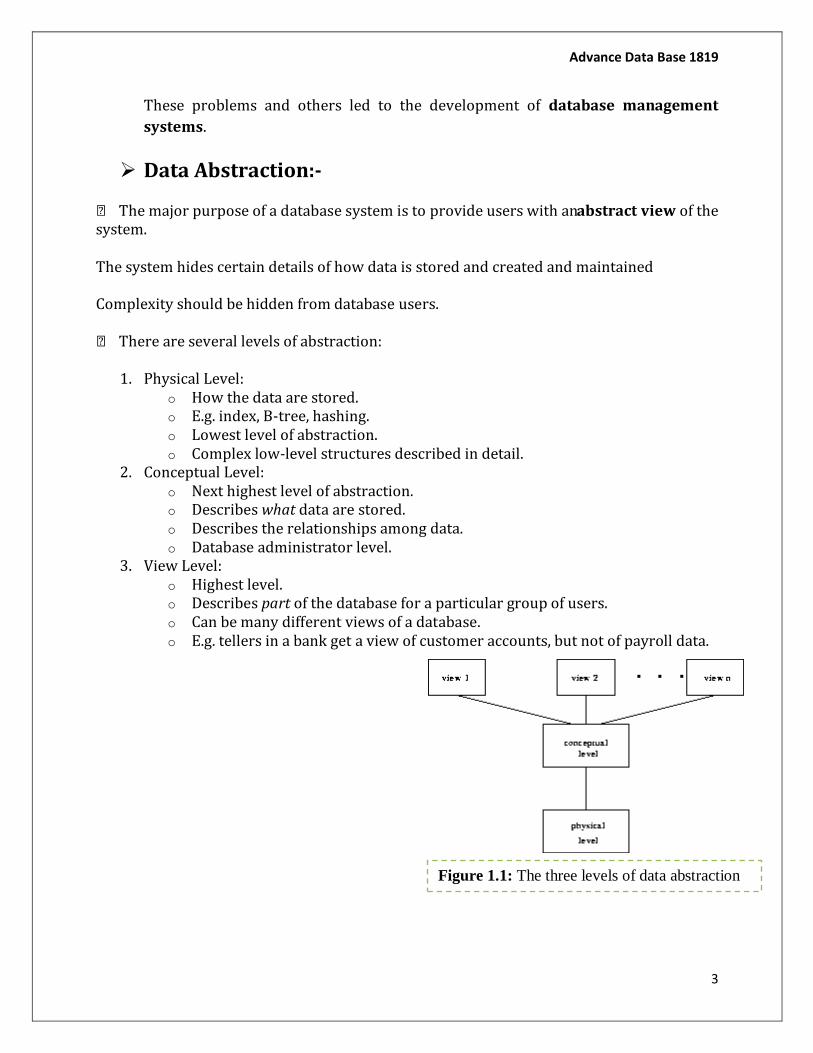
There are several levels of abstraction:
1. Physical Level: o How the data are stored. o E.g. index, B-tree, hashing. o Lowest level of abstraction. o Complex low-level structures described in detail.
2. Conceptual Level: o Next highest level of abstraction. o Describes what data are stored. o Describes the relationships among data. o Database administrator level.
3. View Level: o Highest level. o Describes part of the database for a particular group of users. o Can be many different views of a database. o E.g. tellers in a bank get a view of customer accounts, but not of payroll data.
Figure 1.1: The three levels of data abstraction

Advance Data Base 1819
4
Data Models:-
1. Data models are a collection of conceptual tools for describing data, data relationships, data semantics and data constraints. There are three different groups:
1. Object-based Logical Models. 2. Record-based Logical Models. 3. Physical Data Models.
We'll look at them in more detail now.
Object-based Logical Models
1. Object-based logical models: o Describe data at the conceptual and view levels. o Provide fairly flexible structuring capabilities. o Allow one to specify data constraints explicitly. o Over 30 such models, including
Entity-relationship model. Object-oriented model. Binary model. Semantic data model. Infological model. Functional data model.
2. At this point, we'll take a closer look at the entity-relationship (E-R) and object-oriented models.
The E-R Model
1. The entity-relationship model is based on a perception of the world as consisting of a collection of basic objects (entities) and relationships among these objects.
o An entity is a distinguishable object that exists. o Each entity has associated with it a set of attributes describing it. o E.g. number and balance for an account entity. o A relationship is an association among several entities. o e.g. A cust_acct relationship associates a customer with each account he or she has. o The set of all entities or relationships of the same type is called the entity set or
relationship set. o Another essential element of the E-R diagram is the mapping cardinalities, which
express the number of entities to which another entity can be associated via a relationship set.
We'll see later how well this model works to describe real world situations.
2. The overall logical structure of a database can be expressed graphically by an E-R diagram:
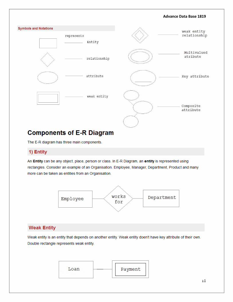
o rectangles: represent entity sets.
Advance Data Base 1819
5
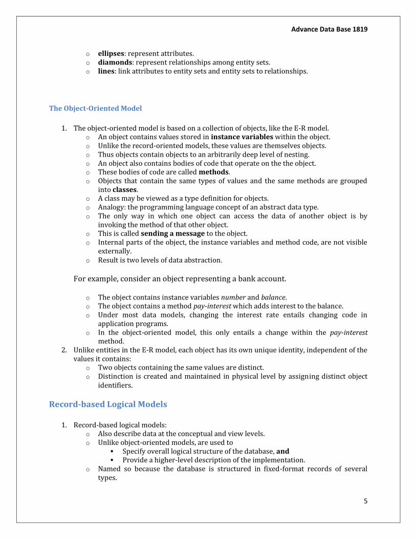
o ellipses: represent attributes. o diamonds: represent relationships among entity sets. o lines: link attributes to entity sets and entity sets to relationships.
The Object-Oriented Model
1. The object-oriented model is based on a collection of objects, like the E-R model. o An object contains values stored in instance variables within the object. o Unlike the record-oriented models, these values are themselves objects. o Thus objects contain objects to an arbitrarily deep level of nesting. o An object also contains bodies of code that operate on the the object. o These bodies of code are called methods. o Objects that contain the same types of values and the same methods are grouped
into classes. o A class may be viewed as a type definition for objects. o Analogy: the programming language concept of an abstract data type. o The only way in which one object can access the data of another object is by
invoking the method of that other object. o This is called sending a message to the object. o Internal parts of the object, the instance variables and method code, are not visible
externally. o Result is two levels of data abstraction.
For example, consider an object representing a bank account.
o The object contains instance variables number and balance. o The object contains a method pay-interest which adds interest to the balance. o Under most data models, changing the interest rate entails changing code in
application programs. o In the object-oriented model, this only entails a change within the pay-interest
method. 2. Unlike entities in the E-R model, each object has its own unique identity, independent of the
values it contains: o Two objects containing the same values are distinct. o Distinction is created and maintained in physical level by assigning distinct object
identifiers.
Record-based Logical Models
1. Record-based logical models: o Also describe data at the conceptual and view levels. o Unlike object-oriented models, are used to
Specify overall logical structure of the database, and Provide a higher-level description of the implementation.
o Named so because the database is structured in fixed-format records of several types.
Advance Data Base 1819
6
o Each record type defines a fixed number of fields, or attributes. o Each field is usually of a fixed length (this simplifies the implementation). o Record-based models do not include a mechanism for direct representation of code
in the database. o Separate languages associated with the model are used to express database queries
and updates. o The three most widely-accepted models are the relational, network, and
hierarchical. o This course will concentrate on the relational model. o The network and hierarchical models are covered in appendices in the text.
The Relational Model
Data and relationships are represented by a collection of tables. Each table has a number of columns with unique names, e.g. customer, account. Figure 1.3 shows a sample relational database.
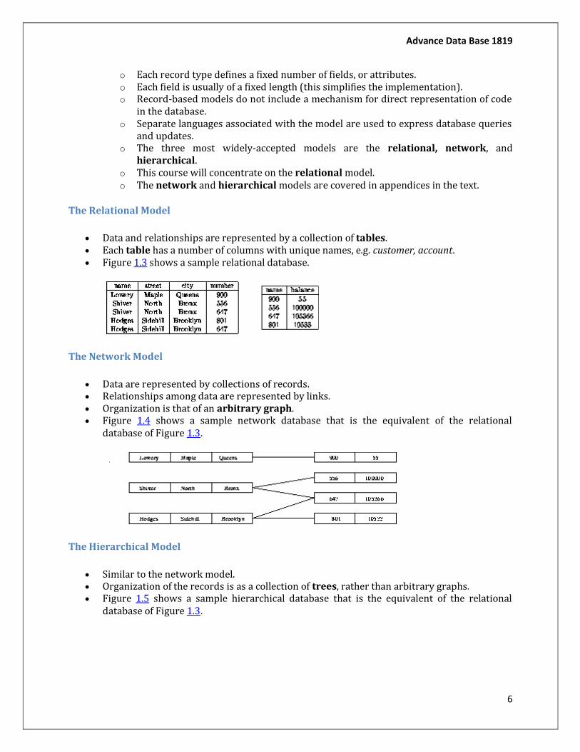
The Network Model
Data are represented by collections of records. Relationships among data are represented by links. Organization is that of an arbitrary graph. Figure 1.4 shows a sample network database that is the equivalent of the relational
database of Figure 1.3.
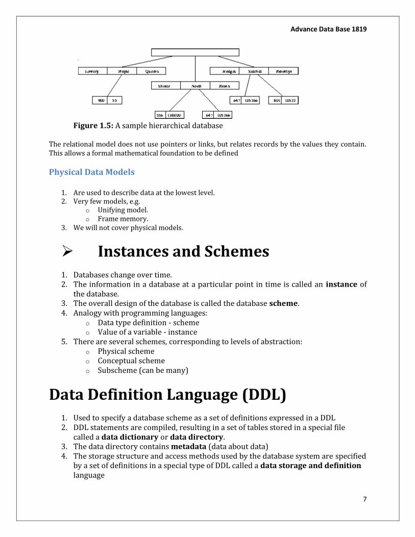
The Hierarchical Model
Similar to the network model. Organization of the records is as a collection of trees, rather than arbitrary graphs. Figure 1.5 shows a sample hierarchical database that is the equivalent of the relational
database of Figure 1.3.
Advance Data Base 1819
7
Figure 1.5: A sample hierarchical database
The relational model does not use pointers or links, but relates records by the values they contain. This allows a formal mathematical foundation to be defined
Physical Data Models
1. Are used to describe data at the lowest level. 2. Very few models, e.g.
o Unifying model. o Frame memory.
3. We will not cover physical models.
Instances and Schemes
1. Databases change over time. 2. The information in a database at a particular point in time is called an instance of
the database. 3. The overall design of the database is called the database scheme. 4. Analogy with programming languages:
o Data type definition - scheme o Value of a variable - instance
5. There are several schemes, corresponding to levels of abstraction: o Physical scheme o Conceptual scheme o Subscheme (can be many)
Data Definition Language (DDL)
1. Used to specify a database scheme as a set of definitions expressed in a DDL 2. DDL statements are compiled, resulting in a set of tables stored in a special file
called a data dictionary or data directory. 3. The data directory contains metadata (data about data) 4. The storage structure and access methods used by the database system are specified
by a set of definitions in a special type of DDL called a data storage and definition language

Advance Data Base 1819
8
5. basic idea: hide implementation details of the database schemes from the users
Data Manipulation Language (DML)
1. Data Manipulation is: o retrieval of information from the database o insertion of new information into the database o deletion of information in the database o modification of information in the database
2. A DML is a language which enables users to access and manipulate data.
The goal is to provide efficient human interaction with the system.
3. There are two types of DML: o procedural: the user specifies what data is needed and how to get it o nonprocedural: the user only specifies what data is needed
Easier for user May not generate code as efficient as that produced by procedural
languages 4. A query language is a portion of a DML involving information retrieval only. The
terms DML and query language are often used synonymously.
Database Manager
1. The database manager is a program module which provides the interface between the low-level data stored in the database and the application programs and queries submitted to the system.
2. Databases typically require lots of storage space (gigabytes). This must be stored on disks. Data is moved between disk and main memory (MM) as needed.
3. The goal of the database system is to simplify and facilitate access to data. Performance is important. Views provide simplification.
4. So the database manager module is responsible for o Interaction with the file manager: Storing raw data on disk using the file
system usually provided by a conventional operating system. The database manager must translate DML statements into low-level file system commands (for storing, retrieving and updating data in the database).
o Integrity enforcement: Checking that updates in the database do not violate consistency constraints (e.g. no bank account balance below $25)
o Security enforcement: Ensuring that users only have access to information they are permitted to see
o Backup and recovery: Detecting failures due to power failure, disk crash, software errors, etc., and restoring the database to its state before the failure
o Concurrency control: Preserving data consistency when there are concurrent users.

Advance Data Base 1819
9
5. Some small database systems may miss some of these features, resulting in simpler database managers. (For example, no concurrency is required on a PC running MS-DOS.) These features are necessary on larger systems.
Database Administrator
1. The database administrator is a person having central control over data and programs accessing that data. Duties of the database administrator include:
o Scheme definition: the creation of the original database scheme. This involves writing a set of definitions in a DDL (data storage and definition language), compiled by the DDL compiler into a set of tables stored in the data dictionary.
o Storage structure and access method definition: writing a set of definitions translated by the data storage and definition language compiler
o Scheme and physical organization modification: writing a set of definitions used by the DDL compiler to generate modifications to appropriate internal system tables (e.g. data dictionary). This is done rarely, but sometimes the database scheme or physical organization must be modified.
o Granting of authorization for data access: granting different types of authorization for data access to various users
o Integrity constraint specification: generating integrity constraints. These are consulted by the database manager module whenever updates occur.
Database Users
1. The database users fall into several categories: o Application programmers are computer professionals interacting with the
system through DML calls embedded in a program written in a host language (e.g. C, PL/1, Pascal).
These programs are called application programs. The DML precompiler converts DML calls (prefaced by a special
character like $, #, etc.) to normal procedure calls in a host language. The host language compiler then generates the object code. Some special types of programming languages combine Pascal-like
control structures with control structures for the manipulation of a database.
These are sometimes called fourth-generation languages. They often include features to help generate forms and display data.
o Sophisticated users interact with the system without writing programs. They form requests by writing queries in a database query language. These are submitted to a query processor that breaks a DML
statement down into instructions for the database manager module.

Advance Data Base 1819
10
o Specialized users are sophisticated users writing special database application programs. These may be CADD systems, knowledge-based and expert systems, complex data systems (audio/video), etc.
o Naive users are unsophisticated users who interact with the system by using permanent application programs (e.g. automated teller machine).
Entity–Relationship model (ER model) is a data model for describing the data or information aspects of a business domain or its process requirements, in an abstract way that lends itself to ultimately being implemented in a database such as a relational database. The main components of ER models are entities (things) and the relationships that can exist among them.
Entity–relationship modeling was developed by Peter Chen and published in a 1976 paper.[1] However, variants of the idea existed previously,[2] and have been devised subsequently such as supertype and subtype data entities[3] and commonality relationships.
Advance Data Base 1819
11
Advance Data Base 1819
12

Advance Data Base 1819
13
Advance Data Base 1819
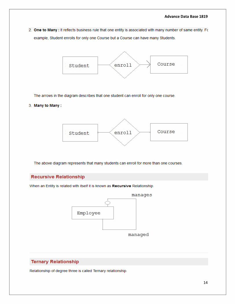
14
Advance Data Base 1819
15
The Relational Model
1. The first database systems were based on the network and hierarchical models. These are covered briefly in appendices in the text. The relational model was first proposed by E.F. Codd in 1970 and the first such systems (notably INGRES and System/R) was developed in 1970s. The relational model is now the dominant model for commercial data processing applications.
2. Note: Attribute Name Abbreviations
The text uses fairly long attribute names which are abbreviated in the notes as follows.
o customer-name becomes cname o customer-city becomes ccity o branch-city becomes bcity o branch-name becomes bname o account-number becomes account# o loan-number becomes loan# o banker-name becomes banker
Structure of Relational Database
1. A relational database consists of a collection of tables, each having a unique name.
A row in a table represents a relationship among a set of values.
Thus a table represents a collection of relationships.
2. There is a direct correspondence between the concept of a table and the mathematical concept of a relation. A substantial theory has been developed for relational databases.

Advance Data Base 1819
16
The Relational Algebra
1. The relational algebra is a procedural query language. o Six fundamental operations:
1. select (unary) 2. project (unary) 3. rename (unary) 4. cartesian product (binary) 5. union (binary) 6. set-difference (binary)
In order to implement a DBMS, there must exist a set of rules which state how the database system will behave. For instance, somewhere in the DBMS must be a set of statements which indicate than when someone inserts data into a row of a relation, it has the effect which the user expects. One way to specify this is to use words to write an `essay' as to how the DBMS will operate, but words tend to be imprecise and open to interpretation. Instead, relational databases are more usually defined using Relational Algebra.
Relational Algebra is :
the formal description of how a relational database operates an interface to the data stored in the database itself the mathematics which underpin SQL operations
Operators in relational algebra are not necessarily the same as SQL operators, even if they have the same name. For example, the SELECT statement exists in SQL, and also exists in relational algebra. These two uses of SELECT are not the same. The DBMS must take whatever SQL statements the user types in and translate them into relational algebra operations before applying them to the database.
Terminology
Relation - a set of tuples. Tuple - a collection of attributes which describe some real world entity. Attribute - a real world role played by a named domain. Domain - a set of atomic values. Set - a mathematical definition for a collection of objects which contains no
duplicates.
Operators - Write
INSERT - provides a list of attribute values for a new tuple in a relation. This operator is the same as SQL.
Advance Data Base 1819
17
DELETE - provides a condition on the attributes of a relation to determine which tuple(s) to remove from the relation. This operator is the same as SQL.
MODIFY - changes the values of one or more attributes in one or more tuples of a relation, as identified by a condition operating on the attributes of the relation. This is equivalent to SQL UPDATE.
Operators - Retrieval
There are two groups of operations:
Mathematical set theory based relations: UNION, INTERSECTION, DIFFERENCE, and CARTESIAN PRODUCT.
Special database operations: SELECT (not the same as SQL SELECT), PROJECT, and JOIN.
Relational SELECT
SELECT is used to obtain a subset of the tuples of a relation that satisfy a select condition.
For example, find all employees born after 1st Jan 1950:
SELECTdob '01/JAN/1950'(employee)
Relational PROJECT
The PROJECT operation is used to select a subset of the attributes of a relation by specifying the names of the required attributes.
For example, to get a list of all employees surnames and employee numbers:
PROJECTsurname,empno(employee)
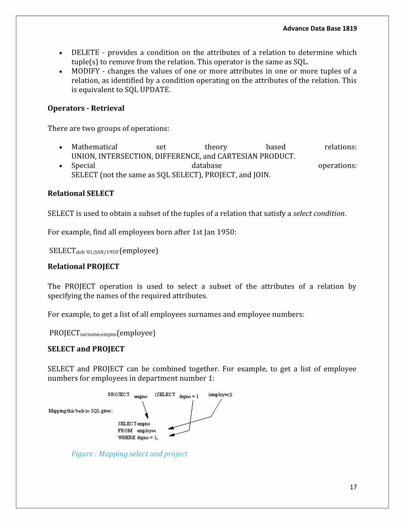
SELECT and PROJECT
SELECT and PROJECT can be combined together. For example, to get a list of employee numbers for employees in department number 1:
Figure : Mapping select and project
Advance Data Base 1819
18
Set Operations - semantics
Consider two relations R and S.
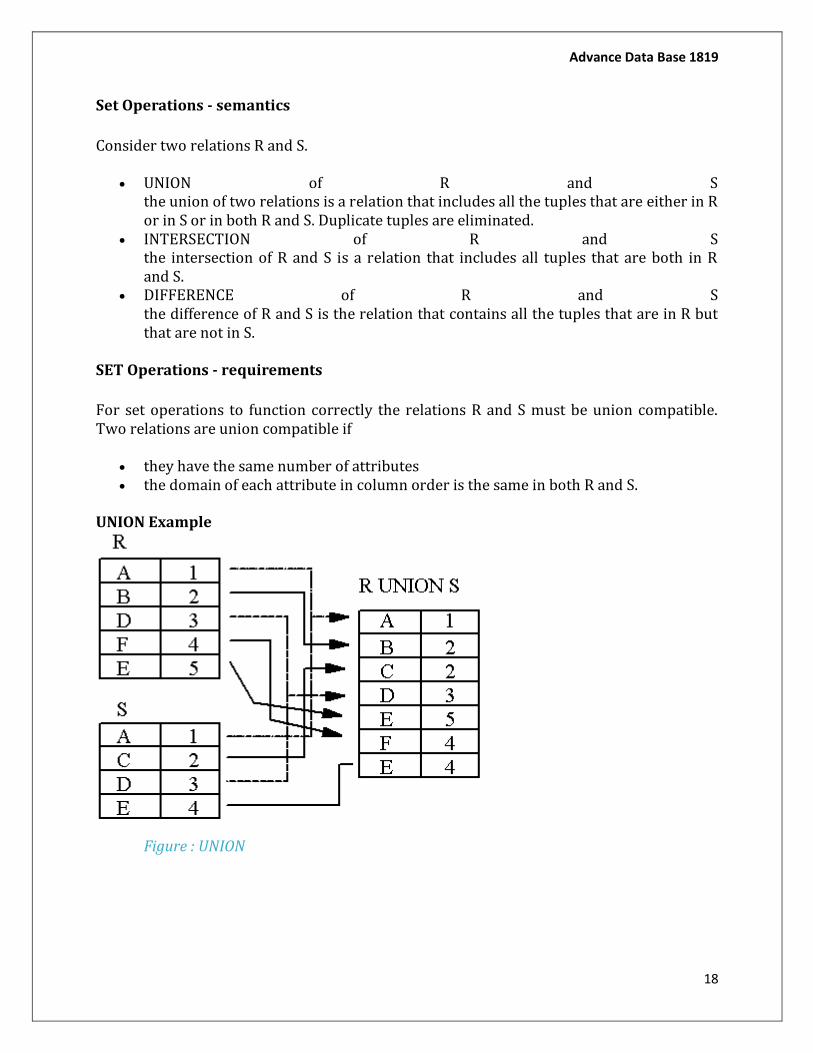
UNION of R and S the union of two relations is a relation that includes all the tuples that are either in R or in S or in both R and S. Duplicate tuples are eliminated.
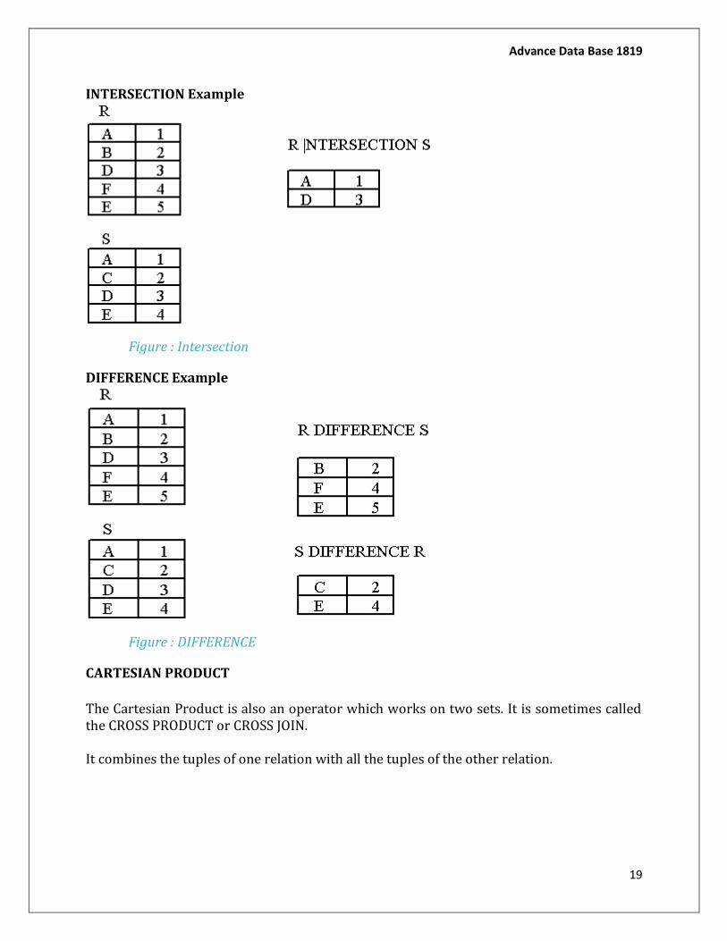
INTERSECTION of R and S the intersection of R and S is a relation that includes all tuples that are both in R and S.
DIFFERENCE of R and S the difference of R and S is the relation that contains all the tuples that are in R but that are not in S.
SET Operations - requirements
For set operations to function correctly the relations R and S must be union compatible. Two relations are union compatible if
they have the same number of attributes the domain of each attribute in column order is the same in both R and S.
UNION Example
Figure : UNION
Advance Data Base 1819
19
INTERSECTION Example
Figure : Intersection
DIFFERENCE Example
Figure : DIFFERENCE
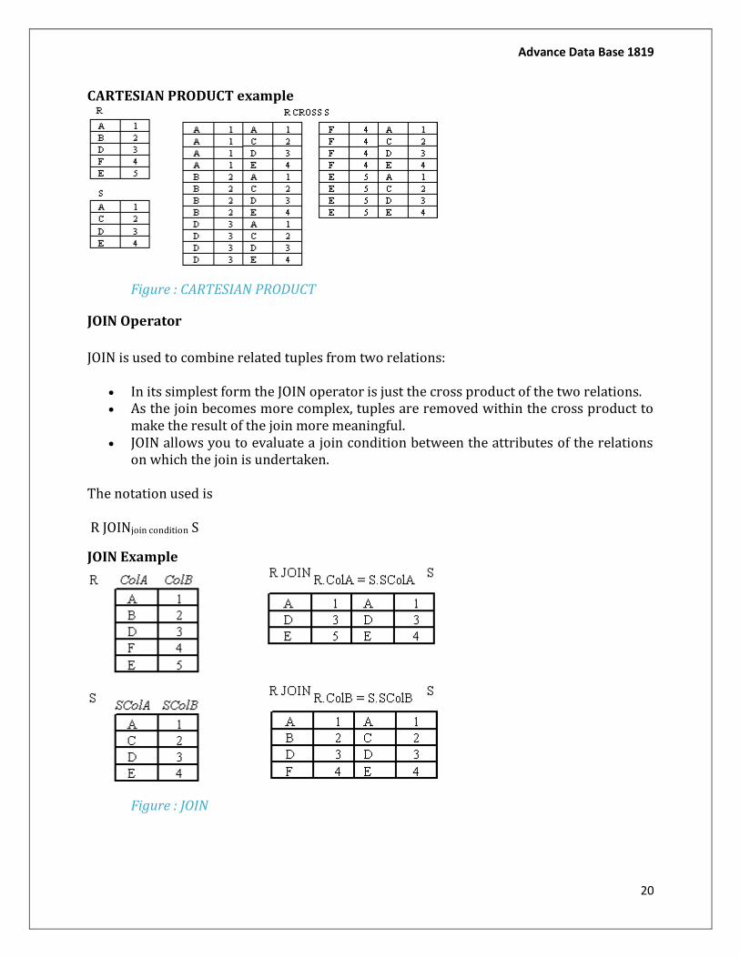
CARTESIAN PRODUCT
The Cartesian Product is also an operator which works on two sets. It is sometimes called the CROSS PRODUCT or CROSS JOIN.
It combines the tuples of one relation with all the tuples of the other relation.
Advance Data Base 1819
20
CARTESIAN PRODUCT example
Figure : CARTESIAN PRODUCT
JOIN Operator
JOIN is used to combine related tuples from two relations:
In its simplest form the JOIN operator is just the cross product of the two relations. As the join becomes more complex, tuples are removed within the cross product to
make the result of the join more meaningful. JOIN allows you to evaluate a join condition between the attributes of the relations
on which the join is undertaken.
The notation used is
R JOINjoin condition S
JOIN Example
Figure : JOIN
Advance Data Base 1819
21
Natural Join
Invariably the JOIN involves an equality test, and thus is often described as an equi-join. Such joins result in two attributes in the resulting relation having exactly the same value. A `natural join' will remove the duplicate attribute(s).
In most systems a natural join will require that the attributes have the same name to identify the attribute(s) to be used in the join. This may require a renaming mechanism.
If you do use natural joins make sure that the relations do not have two attributes with the same name by accident.
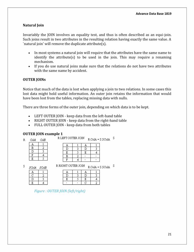
OUTER JOINs
Notice that much of the data is lost when applying a join to two relations. In some cases this lost data might hold useful information. An outer join retains the information that would have been lost from the tables, replacing missing data with nulls.
There are three forms of the outer join, depending on which data is to be kept.
LEFT OUTER JOIN - keep data from the left-hand table RIGHT OUTER JOIN - keep data from the right-hand table FULL OUTER JOIN - keep data from both tables
OUTER JOIN example 1
Figure : OUTER JOIN (left/right)

Advance Data Base 1819
22
OUTER JOIN example 2

Advance Data Base 1819
23
Advance Data Base 1819
24

Advance Data Base 1819
25
Relational Databases: A 30 Second Review
Although there exist many different types of database, we will focus on the most common type—the relational database. A relational database consists of one or more tables, where each table consists of 0 or more records, or rows, of data. The data for each row is organized into discrete units of information, known as fields or columns. When we want to show the fields of a table, let's say the Customers table, we will often show it like this:
Advance Data Base 1819
26
Many of the tables in a database will have relationships, or links, between them, either in a one-to-one or a one-to-many relationship. The connection between the tables is made by a Primary Key – Foreign Key pair, where a Foreign Key field(s) in a given table is the Primary Key of another table. As a typical example, there is a one-to-many relationship between Customers and Orders. Both tables have a CustID field, which is the Primary Key of the Customers table and is a Foreign Key of the Orders Table. The related fields do not need to have the identical name, but it is a good practice to keep them the same.
Fetching Data: SQL SELECT Queries
It is a rare database application that doesn't spend much of its time fetching and displaying data. Once we have data in the database, we want to "slice and dice" it every which way. That is, we want to look at the data and analyze it in an endless number of different ways, constantly varying the filtering, sorting, and calculations that we apply to the raw data. The SQL SELECT statement is what we use to choose, or select, the data that we want returned from the database to our application. It is the language we use to formulate our question, or query, that we want answered by the database. We can start out with very simple queries, but the SELECT statement has many different options and extensions, which provide the great flexibility that we may ultimately need. Our goal is to help you understand the structure and most common elements of a SELECT statement, so that later you will be able to understand the many options and nuances and apply them to your specific needs. We'll start with the bare minimum and slowly add options for greater functionality.
Note: For our illustrations, we will use the Employees table from the Northwind sample database
that has come with MS Access, MS SQL Server and is available for download at the Microsoft
Download Center.
A SQL SELECT statement can be broken down into numerous elements, each beginning with a keyword. Although it is not necessary, common convention is to write these keywords in all capital letters. In this article, we will focus on the most fundamental and common elements of a SELECT statement, namely
SELECT FROM WHERE ORDER BY
The SELECT ... FROM Clause
The most basic SELECT statement has only 2 parts: (1) what columns you want to return and (2) what table(s) those columns come from.
If we want to retrieve all of the information about all of the customers in the Employees table, we could use the asterisk (*) as a shortcut for all of the columns, and our query looks like
Advance Data Base 1819
27
SELECT * FROM Employees
If we want only specific columns (as is usually the case), we can/should explicitly specify them in a comma-separated list, as in
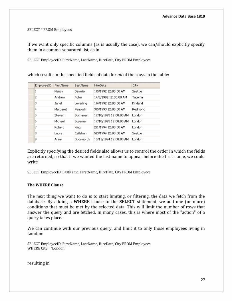
SELECT EmployeeID, FirstName, LastName, HireDate, City FROM Employees
which results in the specified fields of data for all of the rows in the table:
Explicitly specifying the desired fields also allows us to control the order in which the fields are returned, so that if we wanted the last name to appear before the first name, we could write
SELECT EmployeeID, LastName, FirstName, HireDate, City FROM Employees
The WHERE Clause
The next thing we want to do is to start limiting, or filtering, the data we fetch from the database. By adding a WHERE clause to the SELECT statement, we add one (or more) conditions that must be met by the selected data. This will limit the number of rows that answer the query and are fetched. In many cases, this is where most of the "action" of a query takes place.
We can continue with our previous query, and limit it to only those employees living in London:
SELECT EmployeeID, FirstName, LastName, HireDate, City FROM Employees WHERE City = 'London'
resulting in
Advance Data Base 1819
28
If you wanted to get the opposite, the employees who do not live in London, you would write
SELECT EmployeeID, FirstName, LastName, HireDate, City FROM Employees WHERE City <> 'London'
It is not necessary to test for equality; you can also use the standard equality/inequality operators that you would expect. For example, to get a list of employees who where hired on or after a given date, you would write
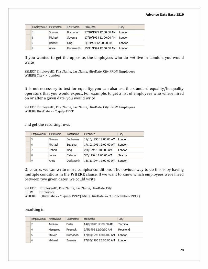
SELECT EmployeeID, FirstName, LastName, HireDate, City FROM Employees WHERE HireDate >= '1-july-1993'
and get the resulting rows
Of course, we can write more complex conditions. The obvious way to do this is by having multiple conditions in the WHERE clause. If we want to know which employees were hired between two given dates, we could write
SELECT EmployeeID, FirstName, LastName, HireDate, City FROM Employees WHERE (HireDate >= '1-june-1992') AND (HireDate <= '15-december-1993')
resulting in

Advance Data Base 1819
29
Note that SQL also has a special BETWEEN operator that checks to see if a value is between two values (including equality on both ends). This allows us to rewrite the previous query as
SELECT EmployeeID, FirstName, LastName, HireDate, City FROM Employees WHERE HireDate BETWEEN '1-june-1992' AND '15-december-1993'
We could also use the NOT operator, to fetch those rows that are not between the specified dates:
SELECT EmployeeID, FirstName, LastName, HireDate, City FROM Employees WHERE HireDate NOT BETWEEN '1-june-1992' AND '15-december-1993'
Let us finish this section on the WHERE clause by looking at two additional, slightly more sophisticated, comparison operators.
What if we want to check if a column value is equal to more than one value? If it is only 2 values, then it is easy enough to test for each of those values, combining them with the OR operator and writing something like
SELECT EmployeeID, FirstName, LastName, HireDate, City FROM Employees WHERE City = 'London' OR City = 'Seattle'
However, if there are three, four, or more values that we want to compare against, the above approach quickly becomes messy. In such cases, we can use the IN operator to test against a set of values. If we wanted to see if the City was either Seattle, Tacoma, or Redmond, we would write
SELECT EmployeeID, FirstName, LastName, HireDate, City FROM Employees WHERE City IN ('Seattle', 'Tacoma', 'Redmond')
producing the results shown below.
As with the BETWEEN operator, here too we can reverse the results obtained and query for those rows where City is not in the specified list:
Advance Data Base 1819
30
SELECT EmployeeID, FirstName, LastName, HireDate, City FROM Employees
WHERE City NOT IN ('Seattle', 'Tacoma', 'Redmond')
Finally, the LIKE operator allows us to perform basic pattern-matching using wildcard characters. For Microsoft SQL Server, the wildcard characters are defined as follows:
Wildcard Description
_
(underscore) matches any single character
% matches a string of one or more characters
[ ] matches any single character within the specified range (e.g. [a-f]) or set (e.g.
[abcdef]).
[^] matches any single character not within the specified range (e.g. [^a-f]) or set (e.g.
[^abcdef]).
A few examples should help clarify these rules.
WHERE FirstName LIKE '_im' finds all three-letter first names that end with 'im' (e.g. Jim, Tim).
WHERE LastName LIKE '%stein' finds all employees whose last name ends with 'stein' WHERE LastName LIKE '%stein%' finds all employees whose last name includes 'stein'
anywhere in the name. WHERE FirstName LIKE '[JT]im' finds three-letter first names that end with 'im' and begin
with either 'J' or 'T' (that is, only Jim and Tim) WHERE LastName LIKE 'm[^c]%' finds all last names beginning with 'm' where the
following (second) letter is not 'c'.
Here too, we can opt to use the NOT operator: to find all of the employees whose first name does not start with 'M' or 'A', we would write
SELECT EmployeeID, FirstName, LastName, HireDate, City FROM Employees WHERE (FirstName NOT LIKE 'M%') AND (FirstName NOT LIKE 'A%')
resulting in

Advance Data Base 1819
31
The ORDER BY Clause
Until now, we have been discussing filtering the data: that is, defining the conditions that determine which rows will be included in the final set of rows to be fetched and returned from the database. Once we have determined which columns and rows will be included in the results of our SELECT query, we may want to control the order in which the rows appear—sorting the data.
To sort the data rows, we include the ORDER BY clause. The ORDER BY clause includes one or more column names that specify the sort order. If we return to one of our first SELECT statements, we can sort its results by City with the following statement:
SELECT EmployeeID, FirstName, LastName, HireDate, City FROM Employees ORDER BY City
By default, the sort order for a column is ascending (from lowest value to highest value), as shown below for the previous query:
If we want the sort order for a column to be descending, we can include the DESC keyword after the column name.
The ORDER BY clause is not limited to a single column. You can include a comma-delimited list of columns to sort by—the rows will all be sorted by the first column specified and then by the next column specified. If we add the Country field to the SELECT clause and want to sort by Country and City, we would write:
Advance Data Base 1819
32
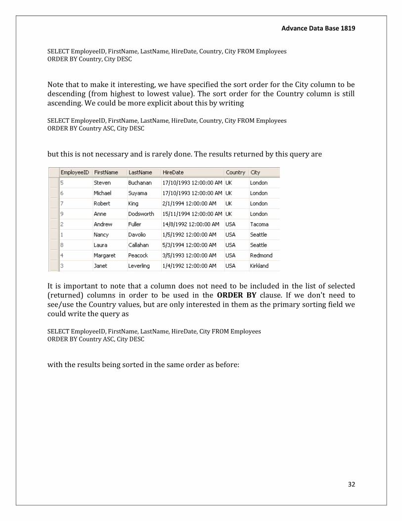
SELECT EmployeeID, FirstName, LastName, HireDate, Country, City FROM Employees ORDER BY Country, City DESC
Note that to make it interesting, we have specified the sort order for the City column to be descending (from highest to lowest value). The sort order for the Country column is still ascending. We could be more explicit about this by writing
SELECT EmployeeID, FirstName, LastName, HireDate, Country, City FROM Employees ORDER BY Country ASC, City DESC
but this is not necessary and is rarely done. The results returned by this query are
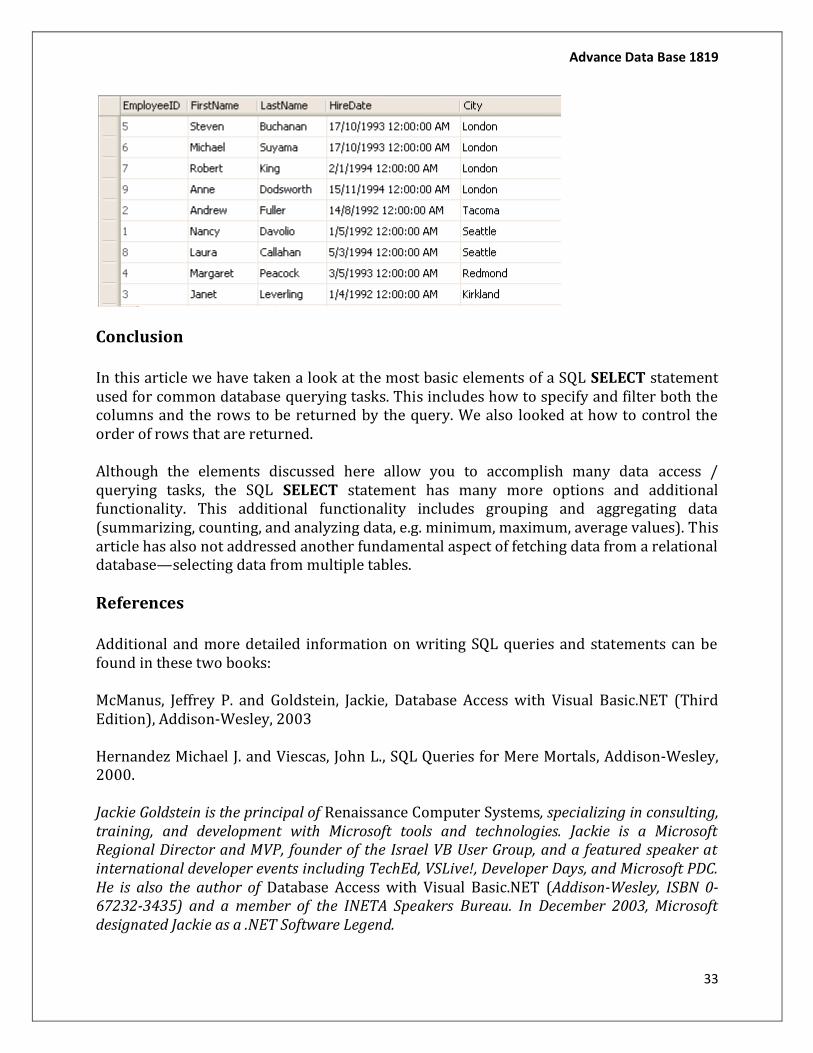
It is important to note that a column does not need to be included in the list of selected (returned) columns in order to be used in the ORDER BY clause. If we don't need to see/use the Country values, but are only interested in them as the primary sorting field we could write the query as
SELECT EmployeeID, FirstName, LastName, HireDate, City FROM Employees ORDER BY Country ASC, City DESC
with the results being sorted in the same order as before:
Advance Data Base 1819
33
Conclusion
In this article we have taken a look at the most basic elements of a SQL SELECT statement used for common database querying tasks. This includes how to specify and filter both the columns and the rows to be returned by the query. We also looked at how to control the order of rows that are returned.
Although the elements discussed here allow you to accomplish many data access / querying tasks, the SQL SELECT statement has many more options and additional functionality. This additional functionality includes grouping and aggregating data (summarizing, counting, and analyzing data, e.g. minimum, maximum, average values). This article has also not addressed another fundamental aspect of fetching data from a relational database—selecting data from multiple tables.
References
Additional and more detailed information on writing SQL queries and statements can be found in these two books:
McManus, Jeffrey P. and Goldstein, Jackie, Database Access with Visual Basic.NET (Third Edition), Addison-Wesley, 2003
Hernandez Michael J. and Viescas, John L., SQL Queries for Mere Mortals, Addison-Wesley, 2000.
Jackie Goldstein is the principal of Renaissance Computer Systems, specializing in consulting, training, and development with Microsoft tools and technologies. Jackie is a Microsoft Regional Director and MVP, founder of the Israel VB User Group, and a featured speaker at international developer events including TechEd, VSLive!, Developer Days, and Microsoft PDC. He is also the author of Database Access with Visual Basic.NET (Addison-Wesley, ISBN 0-67232-3435) and a member of the INETA Speakers Bureau. In December 2003, Microsoft designated Jackie as a .NET Software Legend.

Advance Data Base 1819
34
Nested Quries:-
A Subquery or Inner query or Nested query is a query within another SQL query and embedded within the WHERE clause.
A subquery is used to return data that will be used in the main query as a condition to further restrict the data to be retrieved.
Subqueries can be used with the SELECT, INSERT, UPDATE, and DELETE statements along with the operators like =, <, >, >=, <=, IN, BETWEEN etc.
There are a few rules that subqueries must follow:
Subqueries must be enclosed within parentheses. A subquery can have only one column in the SELECT clause, unless multiple
columns are in the main query for the subquery to compare its selected columns. An ORDER BY cannot be used in a subquery, although the main query can use an
ORDER BY. The GROUP BY can be used to perform the same function as the ORDER BY in a subquery.
Subqueries that return more than one row can only be used with multiple value operators, such as the IN operator.
The SELECT list cannot include any references to values that evaluate to a BLOB, ARRAY, CLOB, or NCLOB.
A subquery cannot be immediately enclosed in a set function. The BETWEEN operator cannot be used with a subquery; however, the BETWEEN
operator can be used within the subquery.
Subqueries with the SELECT Statement:
Subqueries are most frequently used with the SELECT statement. The basic syntax is as follows:
SELECT column_name [, column_name ] FROM table1 [, table2 ] WHERE column_name OPERATOR (SELECT column_name [, column_name ] FROM table1 [, table2 ] [WHERE])
Example:
Consider the CUSTOMERS table having the following records:
Advance Data Base 1819
35
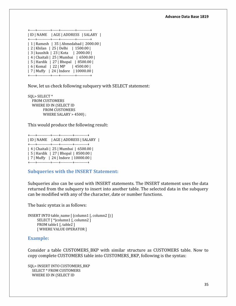
+----+----------+-----+-----------+----------+ | ID | NAME | AGE | ADDRESS | SALARY | +----+----------+-----+-----------+----------+ | 1 | Ramesh | 35 | Ahmedabad | 2000.00 | | 2 | Khilan | 25 | Delhi | 1500.00 | | 3 | kaushik | 23 | Kota | 2000.00 | | 4 | Chaitali | 25 | Mumbai | 6500.00 | | 5 | Hardik | 27 | Bhopal | 8500.00 | | 6 | Komal | 22 | MP | 4500.00 | | 7 | Muffy | 24 | Indore | 10000.00 | +----+----------+-----+-----------+----------+
Now, let us check following subquery with SELECT statement:
SQL> SELECT * FROM CUSTOMERS WHERE ID IN (SELECT ID FROM CUSTOMERS WHERE SALARY > 4500) ;
This would produce the following result:
+----+----------+-----+---------+----------+ | ID | NAME | AGE | ADDRESS | SALARY | +----+----------+-----+---------+----------+ | 4 | Chaitali | 25 | Mumbai | 6500.00 | | 5 | Hardik | 27 | Bhopal | 8500.00 | | 7 | Muffy | 24 | Indore | 10000.00 | +----+----------+-----+---------+----------+
Subqueries with the INSERT Statement:
Subqueries also can be used with INSERT statements. The INSERT statement uses the data returned from the subquery to insert into another table. The selected data in the subquery can be modified with any of the character, date or number functions.
The basic syntax is as follows:
INSERT INTO table_name [ (column1 [, column2 ]) ] SELECT [ *|column1 [, column2 ] FROM table1 [, table2 ] [ WHERE VALUE OPERATOR ]
Example:
Consider a table CUSTOMERS_BKP with similar structure as CUSTOMERS table. Now to copy complete CUSTOMERS table into CUSTOMERS_BKP, following is the syntax:
SQL> INSERT INTO CUSTOMERS_BKP SELECT * FROM CUSTOMERS WHERE ID IN (SELECT ID
Advance Data Base 1819
36
FROM CUSTOMERS) ;
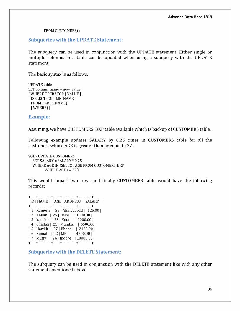
Subqueries with the UPDATE Statement:
The subquery can be used in conjunction with the UPDATE statement. Either single or multiple columns in a table can be updated when using a subquery with the UPDATE statement.
The basic syntax is as follows:
UPDATE table SET column_name = new_value [ WHERE OPERATOR [ VALUE ] (SELECT COLUMN_NAME FROM TABLE_NAME) [ WHERE) ]
Example:
Assuming, we have CUSTOMERS_BKP table available which is backup of CUSTOMERS table.
Following example updates SALARY by 0.25 times in CUSTOMERS table for all the customers whose AGE is greater than or equal to 27:
SQL> UPDATE CUSTOMERS SET SALARY = SALARY * 0.25 WHERE AGE IN (SELECT AGE FROM CUSTOMERS_BKP WHERE AGE >= 27 );
This would impact two rows and finally CUSTOMERS table would have the following records:
+----+----------+-----+-----------+----------+ | ID | NAME | AGE | ADDRESS | SALARY | +----+----------+-----+-----------+----------+ | 1 | Ramesh | 35 | Ahmedabad | 125.00 | | 2 | Khilan | 25 | Delhi | 1500.00 | | 3 | kaushik | 23 | Kota | 2000.00 | | 4 | Chaitali | 25 | Mumbai | 6500.00 | | 5 | Hardik | 27 | Bhopal | 2125.00 | | 6 | Komal | 22 | MP | 4500.00 | | 7 | Muffy | 24 | Indore | 10000.00 | +----+----------+-----+-----------+----------+
Subqueries with the DELETE Statement:
The subquery can be used in conjunction with the DELETE statement like with any other statements mentioned above.
Advance Data Base 1819
37
The basic syntax is as follows:
DELETE FROM TABLE_NAME [ WHERE OPERATOR [ VALUE ] (SELECT COLUMN_NAME FROM TABLE_NAME) [ WHERE) ]
Example:
Assuming, we have CUSTOMERS_BKP table available which is backup of CUSTOMERS table.
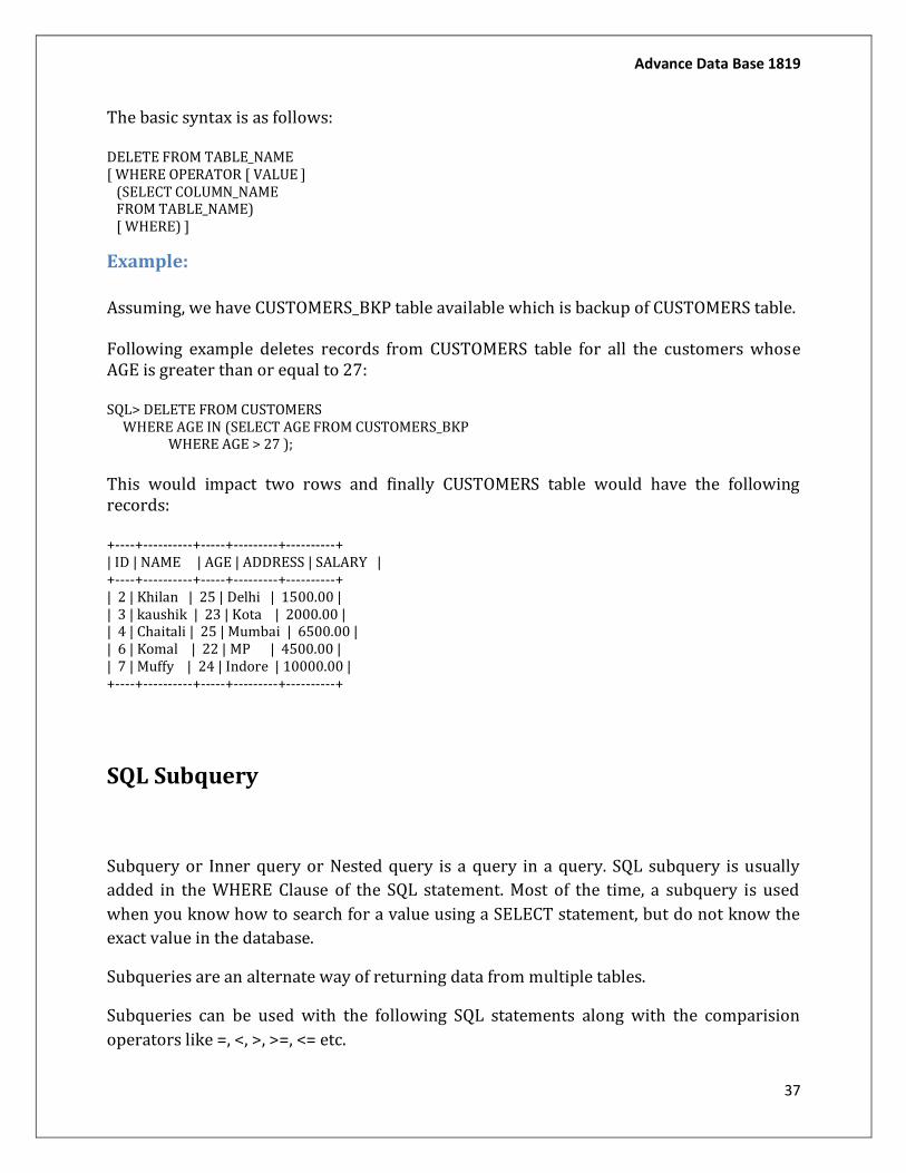
Following example deletes records from CUSTOMERS table for all the customers whose AGE is greater than or equal to 27:
SQL> DELETE FROM CUSTOMERS WHERE AGE IN (SELECT AGE FROM CUSTOMERS_BKP WHERE AGE > 27 );
This would impact two rows and finally CUSTOMERS table would have the following records:
+----+----------+-----+---------+----------+ | ID | NAME | AGE | ADDRESS | SALARY | +----+----------+-----+---------+----------+ | 2 | Khilan | 25 | Delhi | 1500.00 | | 3 | kaushik | 23 | Kota | 2000.00 | | 4 | Chaitali | 25 | Mumbai | 6500.00 | | 6 | Komal | 22 | MP | 4500.00 | | 7 | Muffy | 24 | Indore | 10000.00 | +----+----------+-----+---------+----------+
SQL Subquery
Subquery or Inner query or Nested query is a query in a query. SQL subquery is usually
added in the WHERE Clause of the SQL statement. Most of the time, a subquery is used
when you know how to search for a value using a SELECT statement, but do not know the
exact value in the database.
Subqueries are an alternate way of returning data from multiple tables.
Subqueries can be used with the following SQL statements along with the comparision
operators like =, <, >, >=, <= etc.
Advance Data Base 1819
38
SELECT
INSERT
UPDATE
DELETE
Subquery Example:
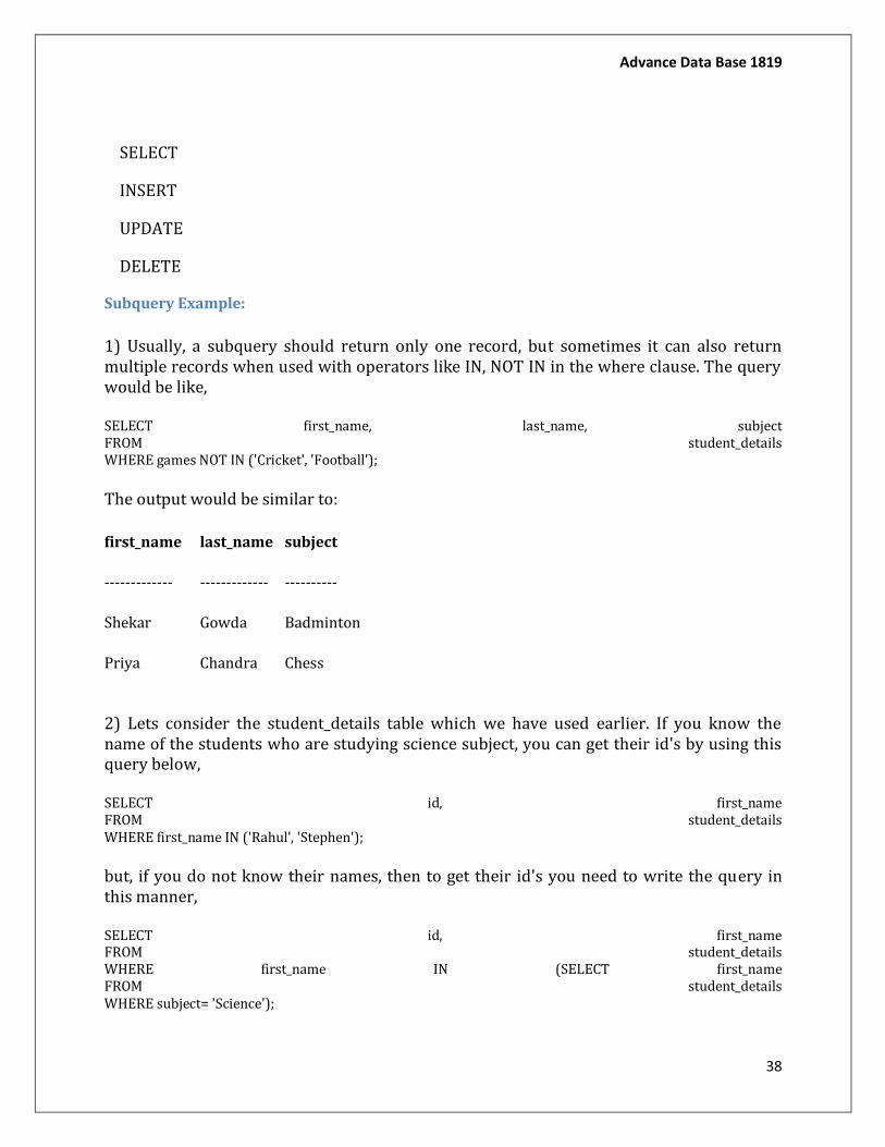
1) Usually, a subquery should return only one record, but sometimes it can also return multiple records when used with operators like IN, NOT IN in the where clause. The query would be like,
SELECT first_name, last_name, subject FROM student_details WHERE games NOT IN ('Cricket', 'Football');
The output would be similar to:
first_name last_name subject
------------- ------------- ----------
Shekar Gowda Badminton
Priya Chandra Chess
2) Lets consider the student_details table which we have used earlier. If you know the name of the students who are studying science subject, you can get their id's by using this query below,
SELECT id, first_name FROM student_details WHERE first_name IN ('Rahul', 'Stephen');
but, if you do not know their names, then to get their id's you need to write the query in this manner,
SELECT id, first_name FROM student_details WHERE first_name IN (SELECT first_name FROM student_details WHERE subject= 'Science');
Advance Data Base 1819
39
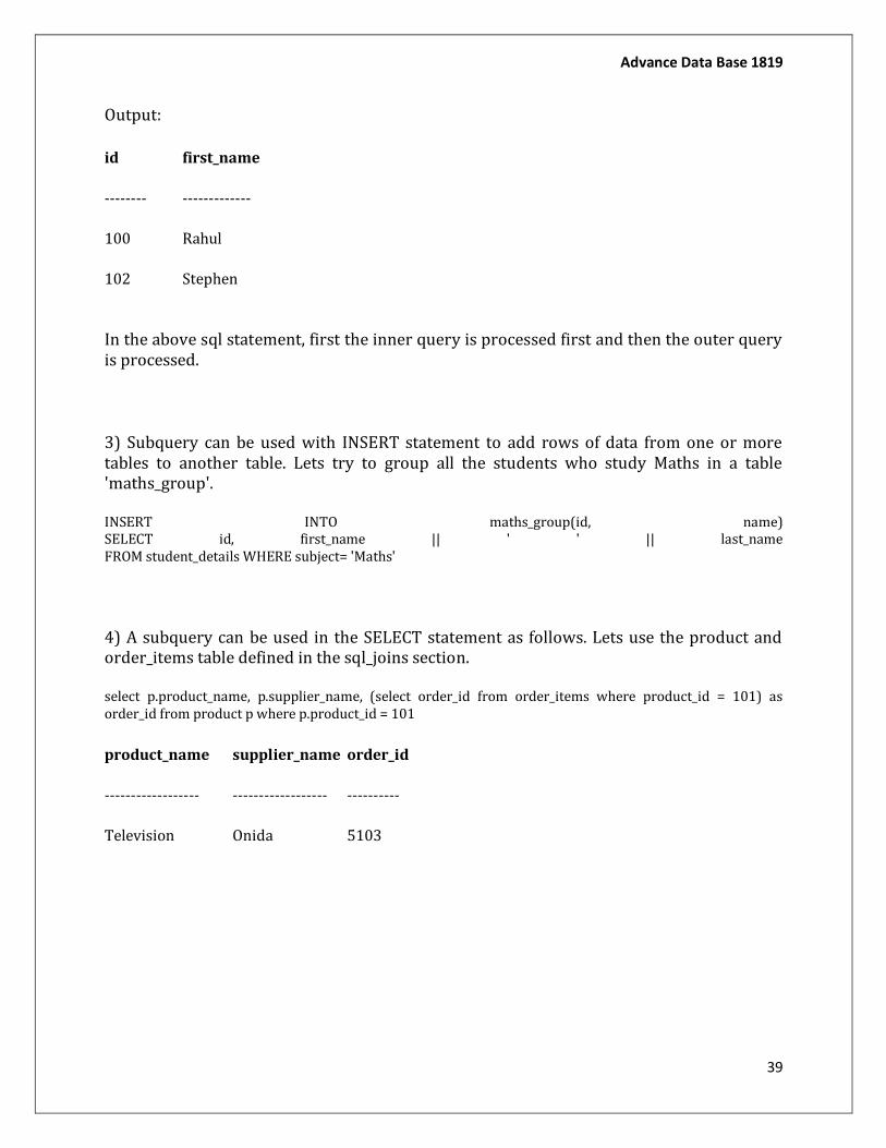
Output:
id first_name
-------- -------------
100 Rahul
102 Stephen
In the above sql statement, first the inner query is processed first and then the outer query is processed.
3) Subquery can be used with INSERT statement to add rows of data from one or more tables to another table. Lets try to group all the students who study Maths in a table 'maths_group'.
INSERT INTO maths_group(id, name) SELECT id, first_name || ' ' || last_name FROM student_details WHERE subject= 'Maths'
4) A subquery can be used in the SELECT statement as follows. Lets use the product and order_items table defined in the sql_joins section.
select p.product_name, p.supplier_name, (select order_id from order_items where product_id = 101) as order_id from product p where p.product_id = 101
product_name supplier_name order_id
------------------ ------------------ ----------
Television Onida 5103
Advance Data Base 1819
40
UNIT-2
Prolems Caused by Redundancy:-
Storing the SeHne inforrnation redundantly, that is, in l110re than one place
\vithin a database, can lead to several problcll1S:
- Redundant Storage: SOU1C iuforInation is stored repeatedly.
- Update Anomalies: If one copy of sueh repeated data is updated, an inconsistency is
created unless all copies cu'c sirnilarly updated.
- Insertion Anomalies: It IIU1Y not be possible to store certain inforlnation unless sorne
other, unrelated, inforIIlatioIl is stored as well.
- Deletion Anomalies: It rnay not be possible to delete certain inforrnation vvithout losing
SOHle other, unrelated, infofrnation as v'lell.
Problems Related to Decomposition lJnless \ve are careful~ decornposing a relation scherna can create 1n01'e problerns
than it solves. rrvVO irnportant questions llHlst be asked repeatedly:
1. 1)0 vve need to decornpose a relation?
2. \\That problerns (if any) does a given deeornposition cause?
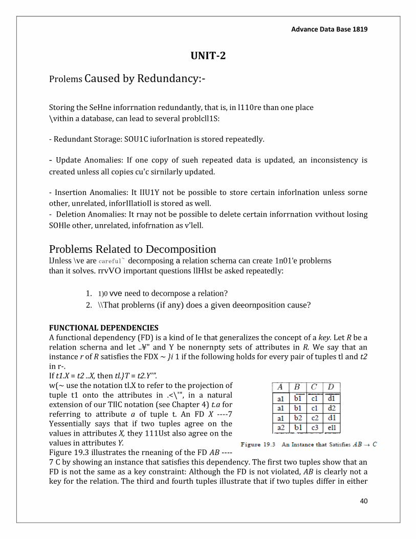
FUNCTIONAL DEPENDENCIES A functional dependency (FD) is a kind of Ie that generalizes the concept of a key. Let R be a relation scherna and let ..¥" and Y be nonernpty sets of attributes in R. We say that an instance r of R satisfies the FDX ~ }i 1 if the following holds for every pair of tuples tl and t2 in r-. If t1.X = t2 ..X, then tl.}T = t2.Y'". w(~ use the notation tl.X to refer to the projection of tuple t1 onto the attributes in .<\'", in a natural extension of our TIlC notation (see Chapter 4) t.a for referring to attribute a of tuple t. An FD X ----7 Yessentially says that if two tuples agree on the values in attributes X, they 111Ust also agree on the values in attributes Y. Figure 19.3 illustrates the rneaning of the FD AB ----7 C by showing an instance that satisfies this dependency. The first two tuples show that an FD is not the same as a key constraint: Although the FD is not violated, AB is clearly not a key for the relation. The third and fourth tuples illustrate that if two tuples differ in either
Advance Data Base 1819
41
the A field or the B field, they can differ in the C field without violating the FD. On the other hand, if we add a tuple (aI, bl, c2, dl) to the instance shown in this figure, the resulting instance would violate the FD; to see this violation, compare the first tuple in the figure with the new tuple.
Decomposition
1. The previous example might seem to suggest that we should decompose schema as much as possible.
Careless decomposition, however, may lead to another form of bad design.
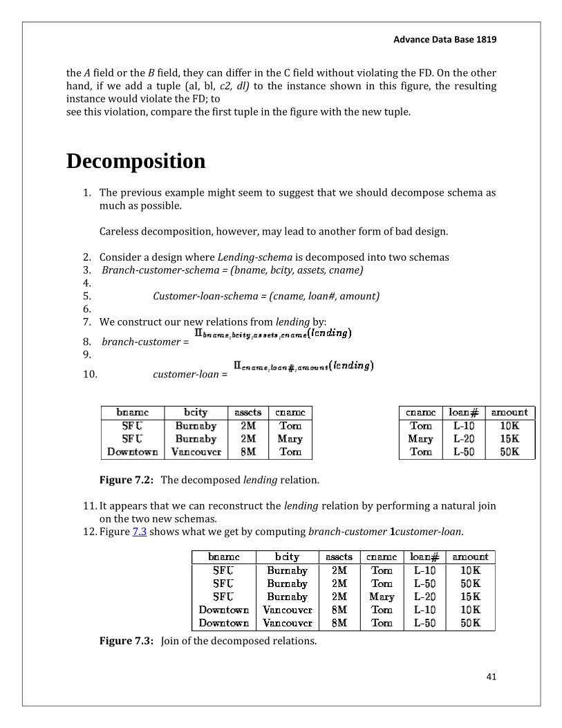
2. Consider a design where Lending-schema is decomposed into two schemas 3. Branch-customer-schema = (bname, bcity, assets, cname) 4. 5. Customer-loan-schema = (cname, loan#, amount) 6. 7. We construct our new relations from lending by:
8. branch-customer = 9.
10. customer-loan =
Figure 7.2: The decomposed lending relation.
11. It appears that we can reconstruct the lending relation by performing a natural join on the two new schemas.
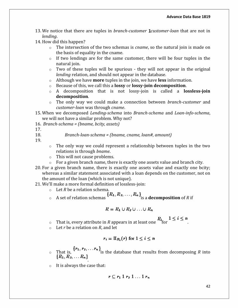
12. Figure 7.3 shows what we get by computing branch-customer customer-loan.
Figure 7.3: Join of the decomposed relations.
Advance Data Base 1819
42
13. We notice that there are tuples in branch-customer customer-loan that are not in lending.
14. How did this happen? o The intersection of the two schemas is cname, so the natural join is made on
the basis of equality in the cname. o If two lendings are for the same customer, there will be four tuples in the
natural join. o Two of these tuples will be spurious - they will not appear in the original
lending relation, and should not appear in the database. o Although we have more tuples in the join, we have less information. o Because of this, we call this a lossy or lossy-join decomposition. o A decomposition that is not lossy-join is called a lossless-join
decomposition. o The only way we could make a connection between branch-customer and
customer-loan was through cname. 15. When we decomposed Lending-schema into Branch-schema and Loan-info-schema,
we will not have a similar problem. Why not? 16. Branch-schema = (bname, bcity, assets) 17. 18. Branch-loan-schema = (bname, cname, loan#, amount) 19.
o The only way we could represent a relationship between tuples in the two relations is through bname.
o This will not cause problems. o For a given branch name, there is exactly one assets value and branch city.
20. For a given branch name, there is exactly one assets value and exactly one bcity; whereas a similar statement associated with a loan depends on the customer, not on the amount of the loan (which is not unique).
21. We'll make a more formal definition of lossless-join: o Let R be a relation schema.
o A set of relation schemas is a decomposition of R if
o That is, every attribute in R appears in at least one for . o Let r be a relation on R, and let
o That is, is the database that results from decomposing R into
. o It is always the case that:
Advance Data Base 1819
43
o To see why this is, consider a tuple .
When we compute the relations , the tuple t gives rise to
one tuple in each . These n tuples combine together to regenerate t when we compute
the natural join of the .
Thus every tuple in r appears in . o However, in general,
o We saw an example of this inequality in our decomposition of lending into branch-customer and customer-loan.
o In order to have a lossless-join decomposition, we need to impose some constraints on the set of possible relations.
o Let C represent a set of constraints on the database.
o A decomposition of a relation schema R is a lossless-join decomposition for R if, for all relations r on schema R that are legal under C:
22. In other words, a lossless-join decomposition is one in which, for any legal relation r, if we decompose r and then ``recompose'' r, we get what we started with - no more and no less.
Lossless-Join Decomposition
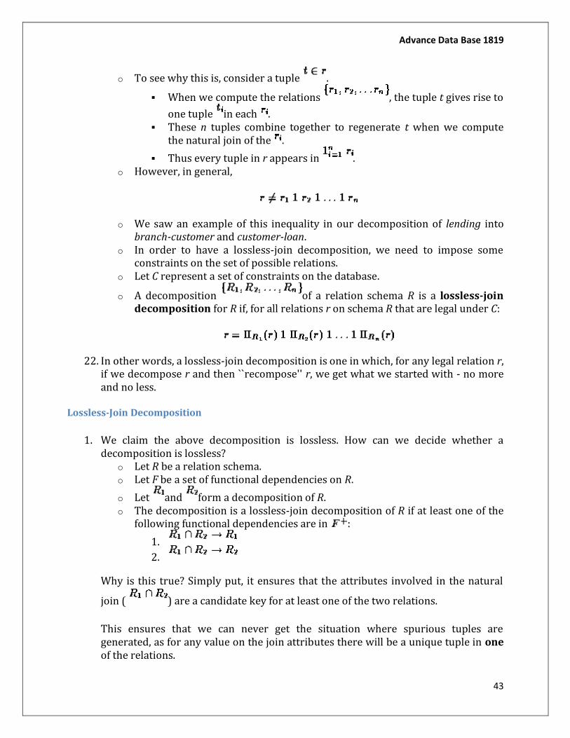
1. We claim the above decomposition is lossless. How can we decide whether a decomposition is lossless?
o Let R be a relation schema. o Let F be a set of functional dependencies on R.
o Let and form a decomposition of R. o The decomposition is a lossless-join decomposition of R if at least one of the
following functional dependencies are in :
1.
2.
Why is this true? Simply put, it ensures that the attributes involved in the natural
join ( ) are a candidate key for at least one of the two relations.
This ensures that we can never get the situation where spurious tuples are generated, as for any value on the join attributes there will be a unique tuple in one of the relations.

Advance Data Base 1819
44
2. We'll now show our decomposition is lossless-join by showing a set of steps that generate the decomposition:
o First we decompose Lending-schema into o Branch-schema = (bname, bcity, assets) o o Loan-info-schema = (bname, cname, loan#, amount) o o Since bname assets bcity, the augmentation rule for functional
dependencies implies that o bname bname assets bcity o o Since Branch-schema Borrow-schema = bname, our decomposition is
lossless join. o Next we decompose Borrow-schema into o Loan-schema = (bname, loan#, amount) o o Borrow-schema = (cname, loan#) o o As loan# is the common attribute, and o loan# amount bname o
This is also a lossless-join decomposition.
Dependency Preservation
1. Another desirable property in database design is dependency preservation. o We would like to check easily that updates to the database do not result in
illegal relations being created. o It would be nice if our design allowed us to check updates without having to
compute natural joins. o To know whether joins must be computed, we need to determine what
functional dependencies may be tested by checking each relation individually.
o Let F be a set of functional dependencies on schema R.
o Let be a decomposition of R.
o The restriction of F to is the set of all functional dependencies in that
include only attributes of . o Functional dependencies in a restriction can be tested in one relation, as they
involve attributes in one relation schema.
o The set of restrictions is the set of dependencies that can be checked efficiently.
Advance Data Base 1819
45
o We need to know whether testing only the restrictions is sufficient.
o Let .
o F' is a set of functional dependencies on schema R, but in general, . o However, it may be that . o If this is so, then every functional dependency in F is implied by F', and if F' is
satisfied, then F must also be satisfied. o A decomposition having the property that is a dependency-
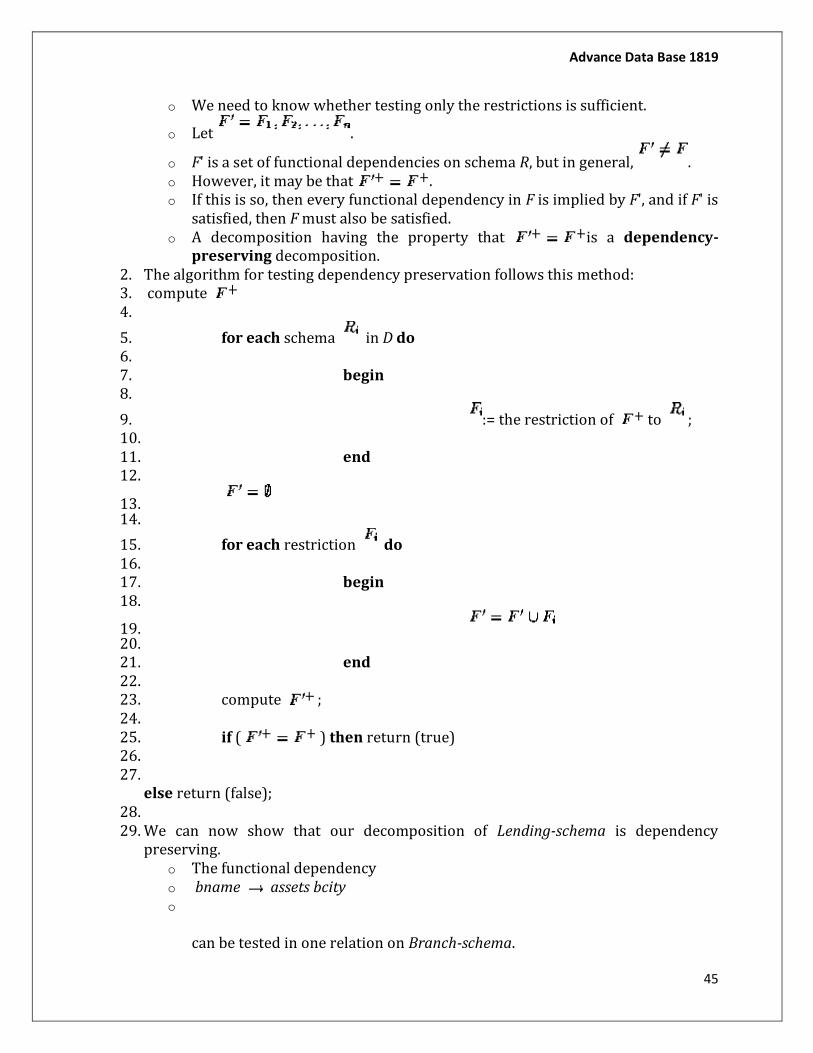
preserving decomposition. 2. The algorithm for testing dependency preservation follows this method: 3. compute 4.
5. for each schema in D do 6. 7. begin 8.
9. := the restriction of to ; 10. 11. end 12.
13. 14.
15. for each restriction do 16. 17. begin 18.
19. 20. 21. end 22. 23. compute ; 24. 25. if ( ) then return (true) 26. 27.
else return (false); 28. 29. We can now show that our decomposition of Lending-schema is dependency
preserving. o The functional dependency o bname assets bcity o
can be tested in one relation on Branch-schema.
Advance Data Base 1819
46
o The functional dependency o loan# amount bname o
can be tested in Loan-schema.
30. As the above example shows, it is often easier not to apply the algorithm shown to test dependency preservation, as computing takes exponential time.
31. An Easier Way To Test For Dependency Preservation
Really we only need to know whether the functional dependencies in F and not in F' are implied by those in F'.
In other words, are the functional dependencies not easily checkable logically implied by those that are?
Rather than compute and , and see whether they are equal, we can do this:
o Find F - F', the functional dependencies not checkable in one relation. o See whether this set is obtainable from F' by using Armstrong's Axioms. o This should take a great deal less work, as we have (usually) just a few
functional dependencies to work on.
Use this simpler method on exams and assignments (unless you have exponential
time available to you).
Normal Forms
A set of rules to avoid redundancy and inconsistency.
Require the concepts of:
o functional dependency (most important: up to BCNF)
o multivalued dependency (4NF)
o join dependency (5NF)
Seven Common Normal Forms: 1NF, 2NF, 3NF, BCNF, 4NF, 5NF, DKNF. (There are
more.)
Higher normal forms are more restrictive.
A relation is in a higher normal form implies that it is in a lower normal form, but not
vice versa.
Assumption: students are already familiar with functional dependencies (FD).
Advance Data Base 1819
47
1.First Normal Form
A relation is in 1NF if all attribute values are atomic: no repeating group, no composite
attributes.
Formally, a relation may only has atomic attributes. Thus, all relations satisfy 1NF.
Example:
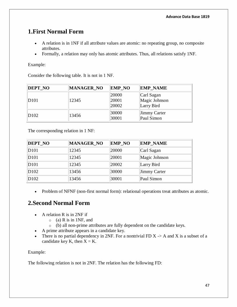
Consider the following table. It is not in 1 NF.
DEPT_NO MANAGER_NO EMP_NO EMP_NAME
D101 12345
20000
20001
20002
Carl Sagan
Magic Johnson
Larry Bird
D102 13456 30000
30001
Jimmy Carter
Paul Simon
The corresponding relation in 1 NF:
DEPT_NO MANAGER_NO EMP_NO EMP_NAME
D101 12345 20000 Carl Sagan
D101 12345 20001 Magic Johnson
D101 12345 20002 Larry Bird
D102 13456 30000 Jimmy Carter
D102 13456 30001 Paul Simon
Problem of NFNF (non-first normal form): relational operations treat attributes as atomic.
2.Second Normal Form
A relation R is in 2NF if
o (a) R is in 1NF, and
o (b) all non-prime attributes are fully dependent on the candidate keys.
A prime attribute appears in a candidate key.
There is no partial dependency in 2NF. For a nontrivial FD X -> A and X is a subset of a
candidate key K, then X = K.
Example:
The following relation is not in 2NF. The relation has the following FD:
Advance Data Base 1819
48
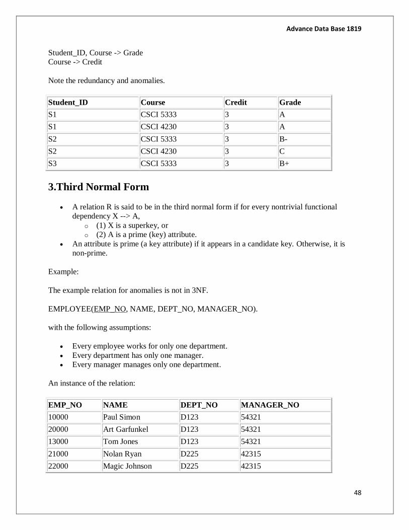
Student_ID, Course -> Grade
Course -> Credit
Note the redundancy and anomalies.
Student_ID Course Credit Grade
S1 CSCI 5333 3 A
S1 CSCI 4230 3 A
S2 CSCI 5333 3 B-
S2 CSCI 4230 3 C
S3 CSCI 5333 3 B+
3.Third Normal Form
A relation R is said to be in the third normal form if for every nontrivial functional
dependency X --> A,
o (1) X is a superkey, or
o (2) A is a prime (key) attribute.
An attribute is prime (a key attribute) if it appears in a candidate key. Otherwise, it is
non-prime.
Example:
The example relation for anomalies is not in 3NF.
EMPLOYEE(EMP_NO, NAME, DEPT_NO, MANAGER_NO).
with the following assumptions:
Every employee works for only one department.
Every department has only one manager.
Every manager manages only one department.
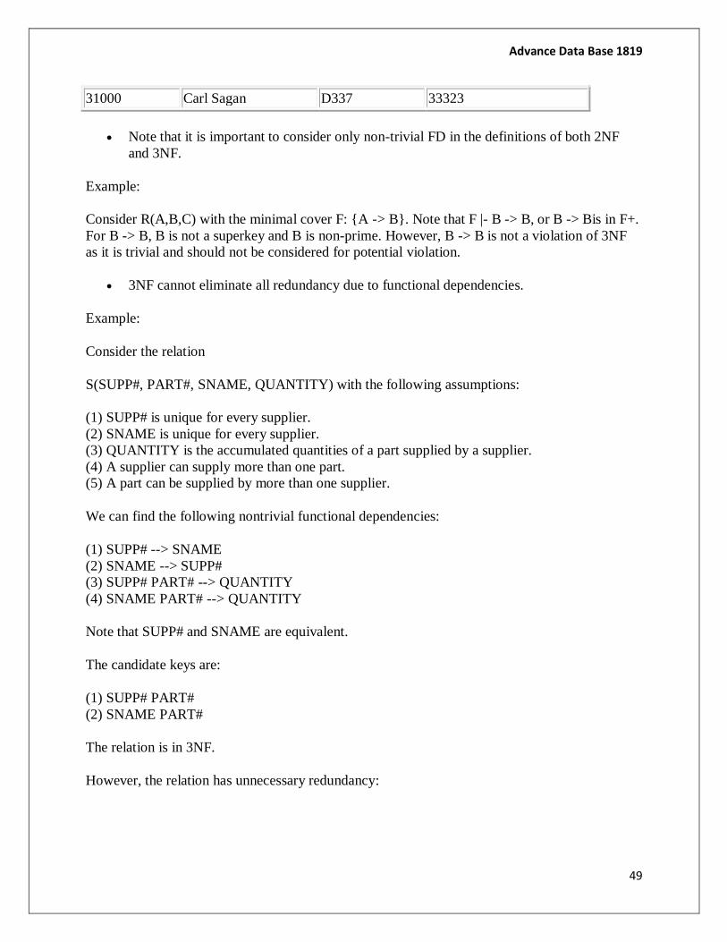
An instance of the relation:
EMP_NO NAME DEPT_NO MANAGER_NO
10000 Paul Simon D123 54321
20000 Art Garfunkel D123 54321
13000 Tom Jones D123 54321
21000 Nolan Ryan D225 42315
22000 Magic Johnson D225 42315
Advance Data Base 1819
49
31000 Carl Sagan D337 33323
Note that it is important to consider only non-trivial FD in the definitions of both 2NF
and 3NF.
Example:
Consider R(A,B,C) with the minimal cover F: {A -> B}. Note that F |- B -> B, or B -> Bis in F+.
For B -> B, B is not a superkey and B is non-prime. However, B -> B is not a violation of 3NF
as it is trivial and should not be considered for potential violation.
3NF cannot eliminate all redundancy due to functional dependencies.
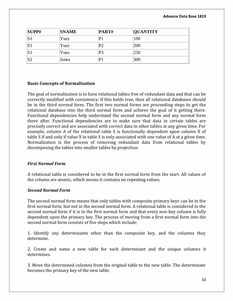
Example:
Consider the relation
S(SUPP#, PART#, SNAME, QUANTITY) with the following assumptions:
(1) SUPP# is unique for every supplier.
(2) SNAME is unique for every supplier.
(3) QUANTITY is the accumulated quantities of a part supplied by a supplier.
(4) A supplier can supply more than one part.
(5) A part can be supplied by more than one supplier.
We can find the following nontrivial functional dependencies:
(1) SUPP# --> SNAME
(2) SNAME --> SUPP#
(3) SUPP# PART# --> QUANTITY
(4) SNAME PART# --> QUANTITY
Note that SUPP# and SNAME are equivalent.
The candidate keys are:
(1) SUPP# PART#
(2) SNAME PART#
The relation is in 3NF.
However, the relation has unnecessary redundancy:
Advance Data Base 1819
50
SUPP# SNAME PART# QUANTITY
S1 Yues P1 100
S1 Yues P2 200
S1 Yues P3 250
S2 Jones P1 300
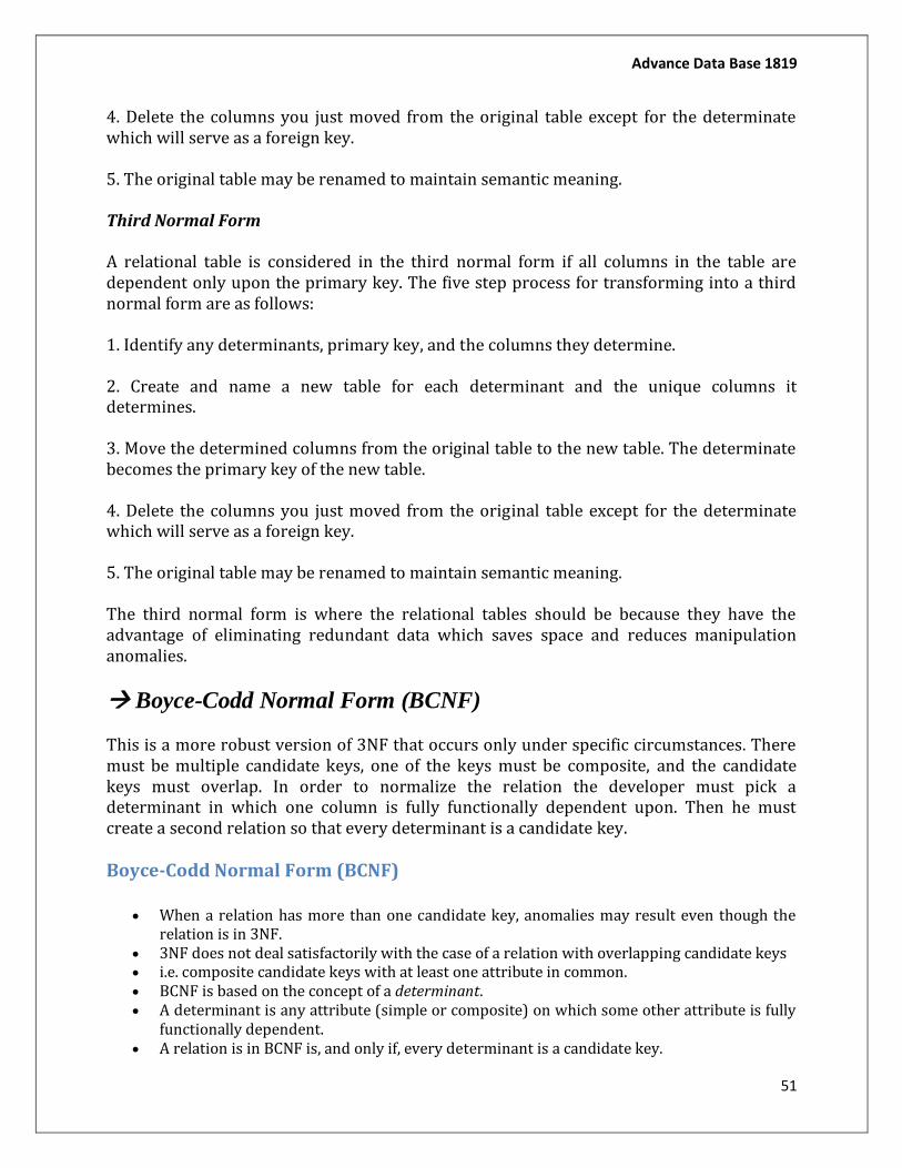
Basic Concepts of Normalization
The goal of normalization is to have relational tables free of redundant data and that can be correctly modified with consistency. If this holds true, then all relational databases should be in the third normal form. The first two normal forms are proceeding steps to get the relational database into the third normal form and achieve the goal of it getting there. Functional dependencies help understand the second normal form and any normal form there after. Functional dependencies are to make sure that data in certain tables are precisely correct and are associated with correct data in other tables at any given time. For example, column A of the relational table S is functionally dependent upon column X of table S if and only if value X in table S is only associated with one value of A at a given time. Normalization is the process of removing redundant data from relational tables by decomposing the tables into smaller tables by projection.
First Normal Form
A relational table is considered to be in the first normal form from the start. All values of the column are atomic, which means it contains no repeating values.
Second Normal Form
The second normal form means that only tables with composite primary keys can be in the first normal form, but not in the second normal form. A relational table is considered in the second normal form if it is in the first normal form and that every non-key column is fully dependent upon the primary key. The process of moving from a first normal form into the second normal form consists of five steps which include:
1. Identify any determinants other than the composite key, and the columns they determine.
2. Create and name a new table for each determinant and the unique columns it determines.
3. Move the determined columns from the original table to the new table. The determinate becomes the primary key of the new table.
Advance Data Base 1819
51
4. Delete the columns you just moved from the original table except for the determinate which will serve as a foreign key.
5. The original table may be renamed to maintain semantic meaning.
Third Normal Form
A relational table is considered in the third normal form if all columns in the table are dependent only upon the primary key. The five step process for transforming into a third normal form are as follows:
1. Identify any determinants, primary key, and the columns they determine.
2. Create and name a new table for each determinant and the unique columns it determines.
3. Move the determined columns from the original table to the new table. The determinate becomes the primary key of the new table.
4. Delete the columns you just moved from the original table except for the determinate which will serve as a foreign key.
5. The original table may be renamed to maintain semantic meaning.
The third normal form is where the relational tables should be because they have the advantage of eliminating redundant data which saves space and reduces manipulation anomalies.
Boyce-Codd Normal Form (BCNF)
This is a more robust version of 3NF that occurs only under specific circumstances. There must be multiple candidate keys, one of the keys must be composite, and the candidate keys must overlap. In order to normalize the relation the developer must pick a determinant in which one column is fully functionally dependent upon. Then he must create a second relation so that every determinant is a candidate key.
Boyce-Codd Normal Form (BCNF)
When a relation has more than one candidate key, anomalies may result even though the relation is in 3NF.
3NF does not deal satisfactorily with the case of a relation with overlapping candidate keys i.e. composite candidate keys with at least one attribute in common. BCNF is based on the concept of a determinant. A determinant is any attribute (simple or composite) on which some other attribute is fully
functionally dependent. A relation is in BCNF is, and only if, every determinant is a candidate key.
Advance Data Base 1819
52
Consider the following relation and determinants.
R(a,b,c,d) a,c -> b,d a,d -> b
Here, the first determinant suggests that the primary key of R could be changed from a,b to a,c. If this change was done all of the non-key attributes present in R could still be determined, and therefore this change is legal. However, the second determinant indicates that a,d determines b, but a,d could not be the key of R as a,d does not determine all of the non key attributes of R (it does not determine c). We would say that the first determinate is a candidate key, but the second determinant is not a candidate key, and thus this relation is not in BCNF (but is in 3rd normal form).
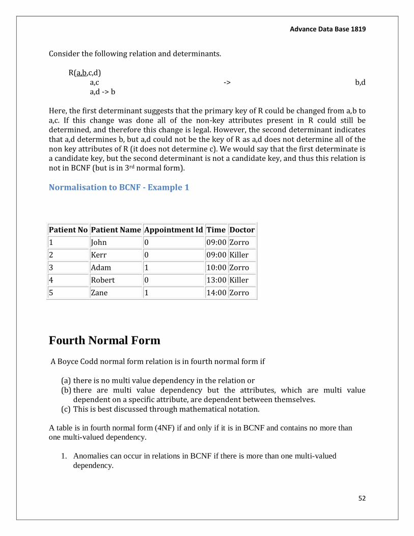
Normalisation to BCNF - Example 1
Patient No Patient Name Appointment Id Time Doctor
1 John 0 09:00 Zorro
2 Kerr 0 09:00 Killer
3 Adam 1 10:00 Zorro
4 Robert 0 13:00 Killer
5 Zane 1 14:00 Zorro
Fourth Normal Form
A Boyce Codd normal form relation is in fourth normal form if
(a) there is no multi value dependency in the relation or (b) there are multi value dependency but the attributes, which are multi value
dependent on a specific attribute, are dependent between themselves. (c) This is best discussed through mathematical notation.
A table is in fourth normal form (4NF) if and only if it is in BCNF and contains no more than
one multi-valued dependency.
1. Anomalies can occur in relations in BCNF if there is more than one multi-valued
dependency.
Advance Data Base 1819
53
2. If A--->B and A--->C but B and C are unrelated, ie A--->(B,C) is false, then we have
more than one multi-valued dependency.
3. A relation is in 4NF when it is in BCNF and has no more than one multi-valued
dependency.
Example to understand 4NF:-
Take the following table structure as an example:
info(employee#, skills, hobbies)
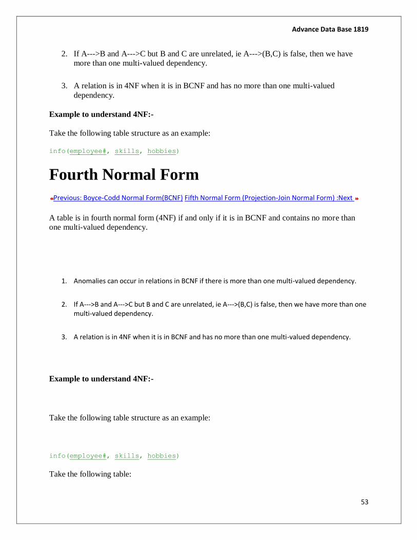
Fourth Normal Form
Previous: Boyce-Codd Normal Form(BCNF) Fifth Normal Form (Projection-Join Normal Form) :Next
A table is in fourth normal form (4NF) if and only if it is in BCNF and contains no more than
one multi-valued dependency.
1. Anomalies can occur in relations in BCNF if there is more than one multi-valued dependency.
2. If A--->B and A--->C but B and C are unrelated, ie A--->(B,C) is false, then we have more than one multi-valued dependency.
3. A relation is in 4NF when it is in BCNF and has no more than one multi-valued dependency.
Example to understand 4NF:-
Take the following table structure as an example:
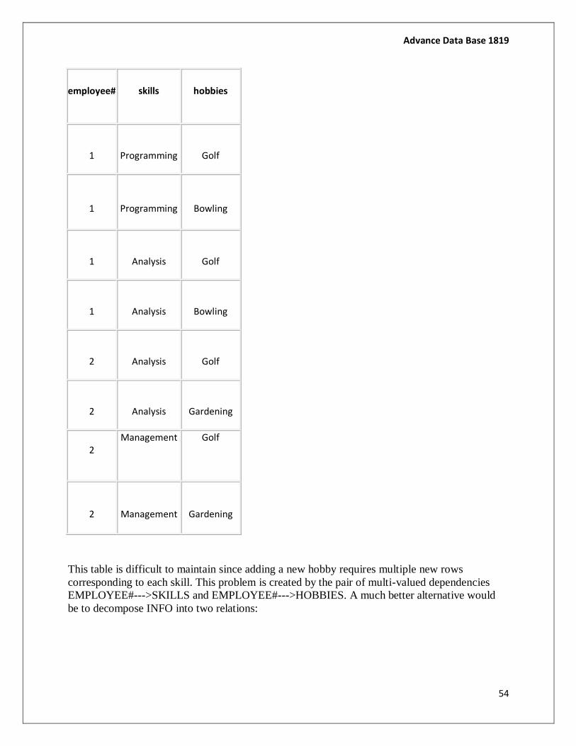
info(employee#, skills, hobbies)
Take the following table:
Advance Data Base 1819
54
employee# skills hobbies
1
Programming
Golf
1
Programming
Bowling
1
Analysis
Golf
1
Analysis
Bowling
2
Analysis
Golf
2
Analysis
Gardening
2 Management
Golf
2
Management
Gardening
This table is difficult to maintain since adding a new hobby requires multiple new rows
corresponding to each skill. This problem is created by the pair of multi-valued dependencies
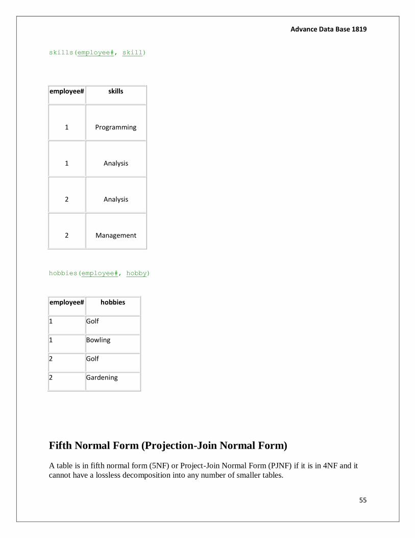
EMPLOYEE#--->SKILLS and EMPLOYEE#--->HOBBIES. A much better alternative would
be to decompose INFO into two relations:
Advance Data Base 1819
55
skills(employee#, skill)
employee# skills
1
Programming
1
Analysis
2
Analysis
2
Management
hobbies(employee#, hobby)
employee# hobbies
1 Golf
1 Bowling
2 Golf
2 Gardening
Fifth Normal Form (Projection-Join Normal Form)
A table is in fifth normal form (5NF) or Project-Join Normal Form (PJNF) if it is in 4NF and it
cannot have a lossless decomposition into any number of smaller tables.
Advance Data Base 1819
56
Properties of 5NF:-
Anomalies can occur in relations in 4NF if the primary key has three or more fields.
5NF is based on the concept of join dependence - if a relation cannot be decomposed any
further then it is in 5NF.
Pair wise cyclical dependency means that:
o You always need to know two values (pair wise).
o For any one you must know the other two (cyclical).
Example to understand 5NF
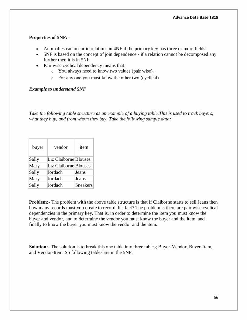
Take the following table structure as an example of a buying table.This is used to track buyers,
what they buy, and from whom they buy. Take the following sample data:
Problem:- The problem with the above table structure is that if Claiborne starts to sell Jeans then
how many records must you create to record this fact? The problem is there are pair wise cyclical
dependencies in the primary key. That is, in order to determine the item you must know the
buyer and vendor, and to determine the vendor you must know the buyer and the item, and
finally to know the buyer you must know the vendor and the item.
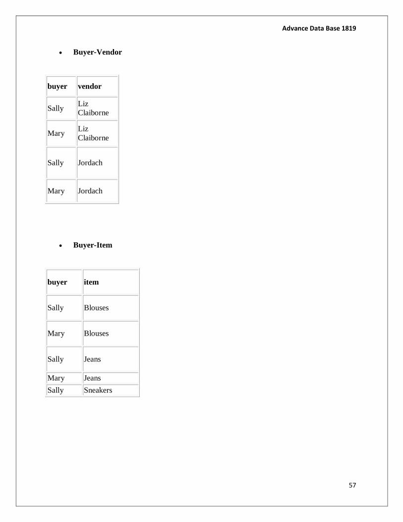
Solution:- The solution is to break this one table into three tables; Buyer-Vendor, Buyer-Item,
and Vendor-Item. So following tables are in the 5NF.
buyer
vendor
item
Sally Liz Claiborne Blouses
Mary Liz Claiborne Blouses
Sally Jordach Jeans
Mary Jordach Jeans
Sally Jordach Sneakers
Advance Data Base 1819
57
Buyer-Vendor
buyer vendor
Sally Liz
Claiborne
Mary Liz
Claiborne
Sally Jordach
Mary Jordach
Buyer-Item
buyer item
Sally Blouses
Mary Blouses
Sally Jeans
Mary Jeans
Sally Sneakers
Advance Data Base 1819
58
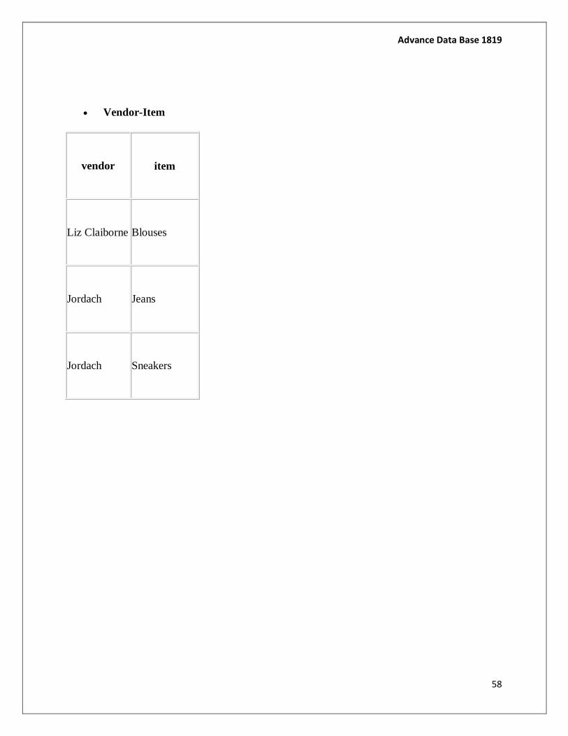
Vendor-Item
vendor
item
Liz Claiborne
Blouses
Jordach
Jeans
Jordach
Sneakers
Advance Data Base 1819
59
UNIT-3
What is a Transaction? A transaction is an event which occurs on the database. Generally a transaction reads a value from the database or writes a value to the database. If you have any concept of Operating Systems, then we can say that a transaction is analogous to processes. Although a transaction can both read and write on the database, there are some fundamental differences between these two classes of operations. A read operation does not change the image of the database in any way. But a write operation, whether performed with the intention of inserting, updating or deleting data from the database, changes the image of the database. That is, we may say that these transactions bring the database from an image which existed before the transaction occurred (called theBefore Image or BFIM) to an image which exists after the transaction occurred (called the After Image or AFIM).
The Four Properties of Transactions Every transaction, for whatever purpose it is being used, has the following four properties. Taking the initial letters of these four properties we collectively call them the The ACID properties
A tomicity: All actions in the Xact happen, or none happen.
C onsistency: If each Xact is consistent, and the DB starts
consistent, it ends up consistent.
I solation: Execution of one Xact is isolated from that of
other Xacts.
D urability: If a Xact commits, its effects persist.
The Recovery Manager guarantees Atomicity & Durability
ACID properties of transactions
In the context of transaction processing, the acronym ACID refers to the four key properties of a transaction: atomicity, consistency, isolation, and durability.
Atomicity
All changes to data are performed as if they are a single operation. That is, all the changes are performed, or none of them are.
Advance Data Base 1819
60
For example, in an application that transfers funds from one account to another, the atomicity property ensures that, if a debit is made successfully from one account, the corresponding credit is made to the other account.
Consistency
Data is in a consistent state when a transaction starts and when it ends.
For example, in an application that transfers funds from one account to another, the consistency property ensures that the total value of funds in both the accounts is the same at the start and end of each transaction.
Isolation
The intermediate state of a transaction is invisible to other transactions. As a result, transactions that run concurrently appear to be serialized.
For example, in an application that transfers funds from one account to another, the isolation property ensures that another transaction sees the transferred funds in one account or the other, but not in both, nor in neither.
Durability
After a transaction successfully completes, changes to data persist and are not undone, even in the event of a system failure.
For example, in an application that transfers funds from one account to another, the durability property ensures that the changes made to each account will not be reversed.
Or
ACID Properties:-
In computer science, ACID (Atomicity, Consistency, Isolation, Durability ) is a set of
properties that guarantee that database transactions are processed reliably. In the context
of databases, a single logical operation on the data is called a transaction. For example, a
transfer of funds from one bank account to another, even involving multiple changes such
as debiting one account and crediting another, is a single transaction.
Jim Gray defined these properties of a reliable transaction system in the late 1970s and
developed technologies to achieve them automatically.
In 1983, Andreas Reuter and Theo Härder coined the acronym ACID to describe them.
Atomicity
Advance Data Base 1819
61
Main article: Atomicity (database systems)
Atomicity requires that each transaction is "all or nothing": if one part of the transaction
fails, the entire transaction fails, and the database state is left unchanged. An atomic system
must guarantee atomicity in each and every situation, including power failures, errors, and
crashes. To the outside world, a committed transaction appears (by its effects on the
database) to be indivisible ("atomic"), and an aborted transaction does not happen.
Consistency
Main article: Consistency (database systems)
The consistency property ensures that any transaction will bring the database from one
valid state to another. Any data written to the database must be valid according to all
defined rules, including but not limited to constraints, cascades, triggers, and any
combination thereof. This does not guarantee correctness of the transaction in all ways the
application programmer might have wanted (that is the responsibility of application-level
code) but merely that any programming errors do not violate any defined rules.
Isolation
Main article: Isolation (database systems)
The isolation property ensures that the concurrent execution of transactions results in a
system state that would be obtained if transactions were executed serially, i.e. one after the
other. Providing isolation is the main goal of concurrency control. Depending on
concurrency control method, the effects of an incomplete transaction might not even be
visible to another transaction.[citation needed]
Durability
Main article: Durability (database systems)
Durability means that once a transaction has been committed, it will remain so, even in the
event of power loss, crashes, or errors. In a relational database, for instance, once a group
of SQL statements execute, the results need to be stored permanently (even if the database
crashes immediately thereafter). To defend against power loss, transactions (or their
effects) must be recorded in a non-volatile memory.
Examples
The following examples further illustrate the ACID properties. In these examples, the
database table has two columns, A and B. An integrity constraint requires that the value in
Advance Data Base 1819
62
A and the value in B must sum to 100. The following SQL code creates a table as described
above:
CREATE TABLE acidtest (A INTEGER, B INTEGER CHECK (A + B = 100));
Atomicity failure
Assume that a transaction attempts to subtract 10 from A and add 10 to B. This is a valid
transaction, since the data continue to satisfy the constraint after it has executed. However,
assume that after removing 10 from A, the transaction is unable to modify B. If the database
retained A's new value, atomicity requires that both parts of this transaction, or neither, be
complete.
Consistency failure
Consistency is a very general term, which demands that the data must meet all validation
rules. In the previous example, the validation is a requirement that A + B = 100. Also, it may
be inferred that both A and B must be integers. A valid range for A and B may also be
inferred. All validation rules must be checked to ensure consistency.
Assume that a transaction attempts to subtract 10 from A without altering B. Because
consistency is checked after each transaction, it is known that A + B = 100 before the
transaction begins. If the transaction removes 10 from A successfully, atomicity will be
achieved. However, a validation check will show that A + B = 90, which is inconsistent with
the rules of the database. The entire transaction must be cancelled and the affected rows
rolled back to their pre-transaction state. If there had been other constraints, triggers, or
cascades, every single change operation would have been checked in the same way as
above before the transaction was committed.
Isolation failure
To demonstrate isolation, we assume two transactions execute at the same time, each
attempting to modify the same data. One of the two must wait until the other completes in
order to maintain isolation.
Consider two transactions. T1 transfers 10 from A to B. T2 transfers 10 from B to A.
Combined, there are four actions:
T1 subtracts 10 from A.
T1 adds 10 to B.
T2 subtracts 10 from B.
Advance Data Base 1819
63
T2 adds 10 to A.
If these operations are performed in order, isolation is maintained, although T2 must wait.
Consider what happens if T1 fails half-way through. The database eliminates T1's effects,
and T2 sees only valid data.
By interleaving the transactions, the actual order of actions might be:
T1 subtracts 10 from A.
T2 subtracts 10 from B.
T2 adds 10 to A.
T1 adds 10 to B.
Again, consider what happens if T1 fails halfway through. By the time T1 fails, T2 has
already modified A; it cannot be restored to the value it had before T1 without leaving an
invalid database. This is known as a write-write failure,[citation needed] because two
transactions attempted to write to the same data field. In a typical system, the problem
would be resolved by reverting to the last known good state, canceling the failed
transaction T1, and restarting the interrupted transaction T2 from the good state.
Durability failure
Assume that a transaction transfers 10 from A to B. It removes 10 from A. It then adds 10 to
B. At this point, a "success" message is sent to the user. However, the changes are still
queued in the disk buffer waiting to be committed to the disk. Power fails and the changes
are lost. The user assumes (understandably) that the changes have been made.
Locking-based Concurrency Control Protocols
This section introduces the details of locking-based concurrency control algorithms. To ensure serializability of concurrent transactions locking methods are the most widely used approach. In this approach, before accessing any data item, a transaction must acquire a lock on that data item. When a transaction acquires a lock on a particular data item, the lock prevents another transaction from modifying that data item. Based on the facts that read-read operation by two different transactions is non-conflicting and the main objective of the locking-based concurrency control techniques is to synchronize the conflicting operations of conflicting transactions, there are two types of locking modes:read lock (also called shared lock) and write lock (also called exclusive lock). If a transaction obtains a read lock on a data item, it can read, but cannot update that data item. On the other hand, if a transaction obtains a write lock on a data item, it can read as well as update that data item. When a transaction obtains a read lock on a particular data item, other transactions are allowed to read that data item because read-read operation is non-conflicting. Thus,
Advance Data Base 1819
64
several transactions can acquire shared lock or read lock on the same data item simultaneously. When a transaction achieves an exclusive lock on a particular data item, no other transactions are allowed to read or update that data item, as read-write and write-write operations are conflicting. A transaction can acquire locks on data items of various sizes, ranging from the entire database down to a data field. The size of the data item determines the fineness or granularity of the lock.
In a distributed database system, the lock manager or scheduler is responsible for managing locks for different transactions that are running on that system. When any transaction requires read or write lock on data items, the transaction manager passes this request to the lock manager. It is the responsibility of the lock manager to check whether that data item is currently locked by another transaction or not. If the data item is locked by another transaction and the existing locking mode is incompatible with the lock requested by the current transaction, the lock manager does not allow the current transaction to obtain the lock; hence, the current transaction is delayed until the existing lock is released. Otherwise, the lock manager permits the current transaction to obtain the desired lock and the information is passed to the transaction manager. In addition to these rules, some systems initially allow the current transaction to acquire a read lock on a data item, if that is compatible with the existing lock, and later the lock is converted into a write lock. This is called upgradation of lock. The level of concurrency increases by upgradation of locking. Similarly, to allow maximum concurrency some systems permit the current transaction to acquire a write lock on a data item, and later the lock is converted into a read lock; this is called downgradation of lock.
Locks
When one thread of control wants to obtain access to an object, it requests a lock for that object. This lock is what allows JE to provide your application with its transactional isolation guarantees by ensuring that:
no other thread of control can read that object (in the case of an exclusive lock), and no other thread of control can modify that object (in the case of an exclusive or non-
exclusive lock).
Lock Resources
When locking occurs, there are conceptually three resources in use:
1. The locker.
This is the thing that holds the lock. In a transactional application, the locker is a transaction handle. For non-transactional operations, the locker is the current thread.
2. The lock.
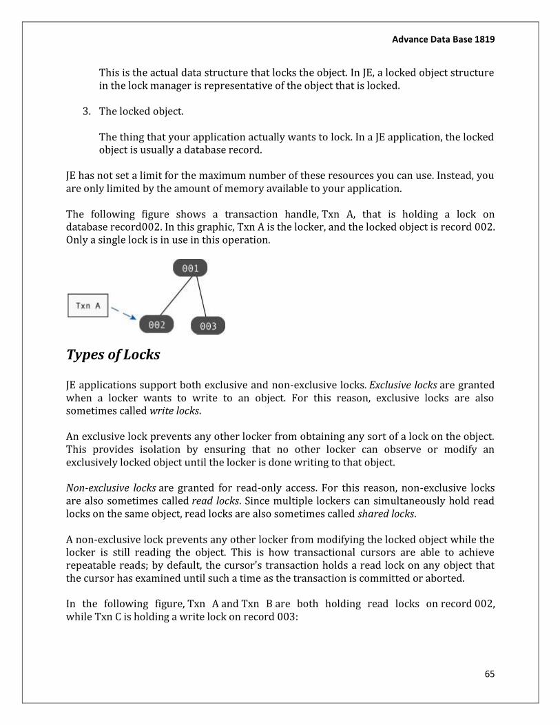
Advance Data Base 1819
65
This is the actual data structure that locks the object. In JE, a locked object structure in the lock manager is representative of the object that is locked.
3. The locked object.
The thing that your application actually wants to lock. In a JE application, the locked object is usually a database record.
JE has not set a limit for the maximum number of these resources you can use. Instead, you are only limited by the amount of memory available to your application.
The following figure shows a transaction handle, Txn A, that is holding a lock on database record002. In this graphic, Txn A is the locker, and the locked object is record 002. Only a single lock is in use in this operation.
Types of Locks
JE applications support both exclusive and non-exclusive locks. Exclusive locks are granted when a locker wants to write to an object. For this reason, exclusive locks are also sometimes called write locks.
An exclusive lock prevents any other locker from obtaining any sort of a lock on the object. This provides isolation by ensuring that no other locker can observe or modify an exclusively locked object until the locker is done writing to that object.
Non-exclusive locks are granted for read-only access. For this reason, non-exclusive locks are also sometimes called read locks. Since multiple lockers can simultaneously hold read locks on the same object, read locks are also sometimes called shared locks.
A non-exclusive lock prevents any other locker from modifying the locked object while the locker is still reading the object. This is how transactional cursors are able to achieve repeatable reads; by default, the cursor's transaction holds a read lock on any object that the cursor has examined until such a time as the transaction is committed or aborted.
In the following figure, Txn A and Txn B are both holding read locks on record 002, while Txn C is holding a write lock on record 003:
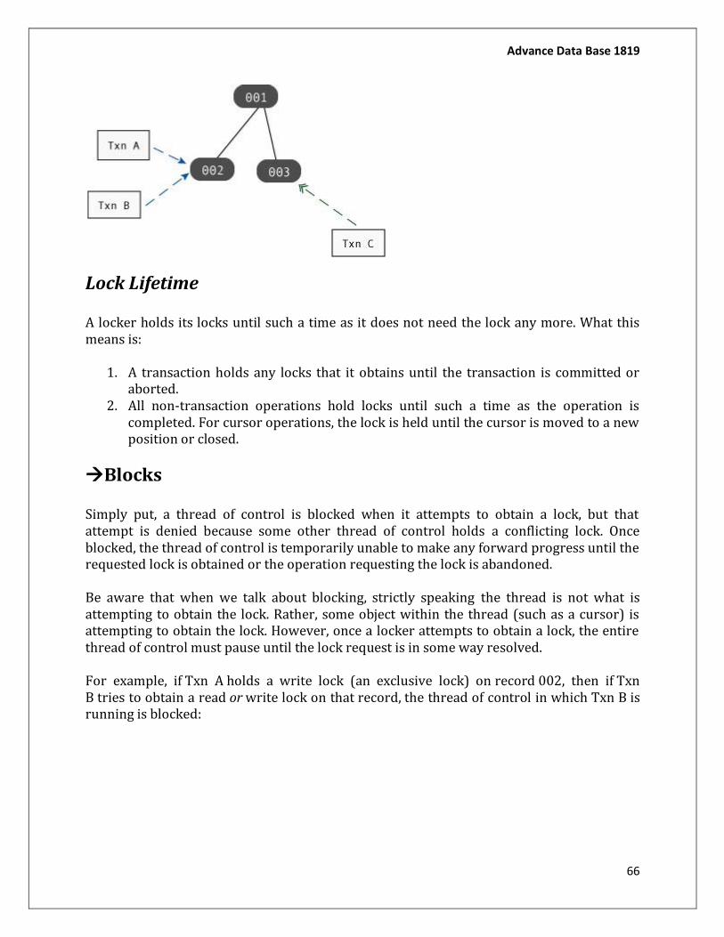
Advance Data Base 1819
66
Lock Lifetime
A locker holds its locks until such a time as it does not need the lock any more. What this means is:
1. A transaction holds any locks that it obtains until the transaction is committed or aborted.
2. All non-transaction operations hold locks until such a time as the operation is completed. For cursor operations, the lock is held until the cursor is moved to a new position or closed.
Blocks
Simply put, a thread of control is blocked when it attempts to obtain a lock, but that attempt is denied because some other thread of control holds a conflicting lock. Once blocked, the thread of control is temporarily unable to make any forward progress until the requested lock is obtained or the operation requesting the lock is abandoned.
Be aware that when we talk about blocking, strictly speaking the thread is not what is attempting to obtain the lock. Rather, some object within the thread (such as a cursor) is attempting to obtain the lock. However, once a locker attempts to obtain a lock, the entire thread of control must pause until the lock request is in some way resolved.
For example, if Txn A holds a write lock (an exclusive lock) on record 002, then if Txn B tries to obtain a read or write lock on that record, the thread of control in which Txn B is running is blocked:
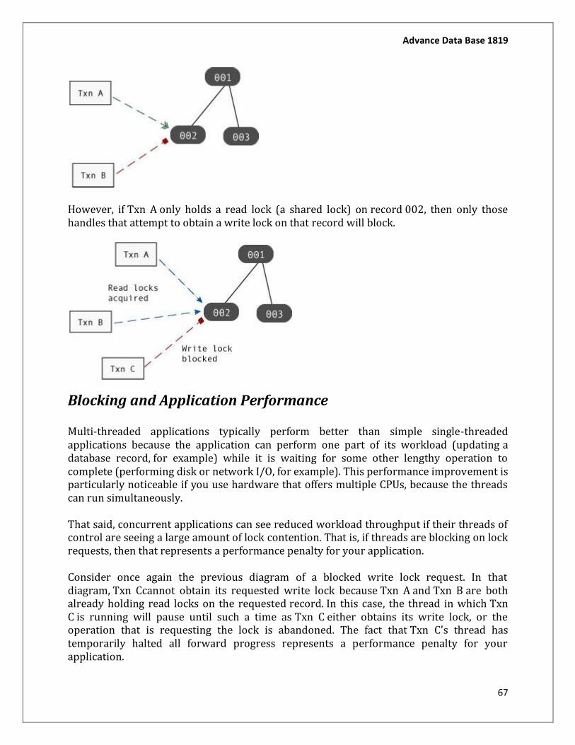
Advance Data Base 1819
67
However, if Txn A only holds a read lock (a shared lock) on record 002, then only those handles that attempt to obtain a write lock on that record will block.
Blocking and Application Performance
Multi-threaded applications typically perform better than simple single-threaded applications because the application can perform one part of its workload (updating a database record, for example) while it is waiting for some other lengthy operation to complete (performing disk or network I/O, for example). This performance improvement is particularly noticeable if you use hardware that offers multiple CPUs, because the threads can run simultaneously.
That said, concurrent applications can see reduced workload throughput if their threads of control are seeing a large amount of lock contention. That is, if threads are blocking on lock requests, then that represents a performance penalty for your application.
Consider once again the previous diagram of a blocked write lock request. In that diagram, Txn Ccannot obtain its requested write lock because Txn A and Txn B are both already holding read locks on the requested record. In this case, the thread in which Txn C is running will pause until such a time as Txn C either obtains its write lock, or the operation that is requesting the lock is abandoned. The fact that Txn C's thread has temporarily halted all forward progress represents a performance penalty for your application.

Advance Data Base 1819
68
Moreover, any read locks that are requested while Txn C is waiting for its write lock will also block until such a time as Txn C has obtained and subsequently released its write lock.
Avoiding Blocks
Reducing lock contention is an important part of performance tuning your concurrent JE application. Applications that have multiple threads of control obtaining exclusive (write) locks are prone to contention issues. Moreover, as you increase the numbers of lockers and as you increase the time that a lock is held, you increase the chances of your application seeing lock contention.
As you are designing your application, try to do the following in order to reduce lock contention:
Reduce the length of time your application holds locks.
Shorter lived transactions will result in shorter lock lifetimes, which will in turn help to reduce lock contention.
In addition, by default transactional cursors hold read locks until such a time as the transaction is completed. For this reason, try to minimize the time you keep transactional cursors opened, or reduce your isolation levels – see below.
If possible, access heavily accessed (read or write) items toward the end of the transaction. This reduces the amount of time that a heavily used record is locked by the transaction.
Reduce your application's isolation guarantees.
By reducing your isolation guarantees, you reduce the situations in which a lock can block another lock. Try using uncommitted reads for your read operations in order to prevent a read lock being blocked by a write lock.
In addition, for cursors you can use degree 2 (read committed) isolation, which causes the cursor to release its read locks as soon as it is done reading the record (as opposed to holding its read locks until the transaction ends).
Be aware that reducing your isolation guarantees can have adverse consequences for your application. Before deciding to reduce your isolation, take care to examine your application's isolation requirements. For information on isolation levels, see Isolation.
Consider your data access patterns.
Depending on the nature of your application, this may be something that you can not do anything about. However, if it is possible to create your threads such that
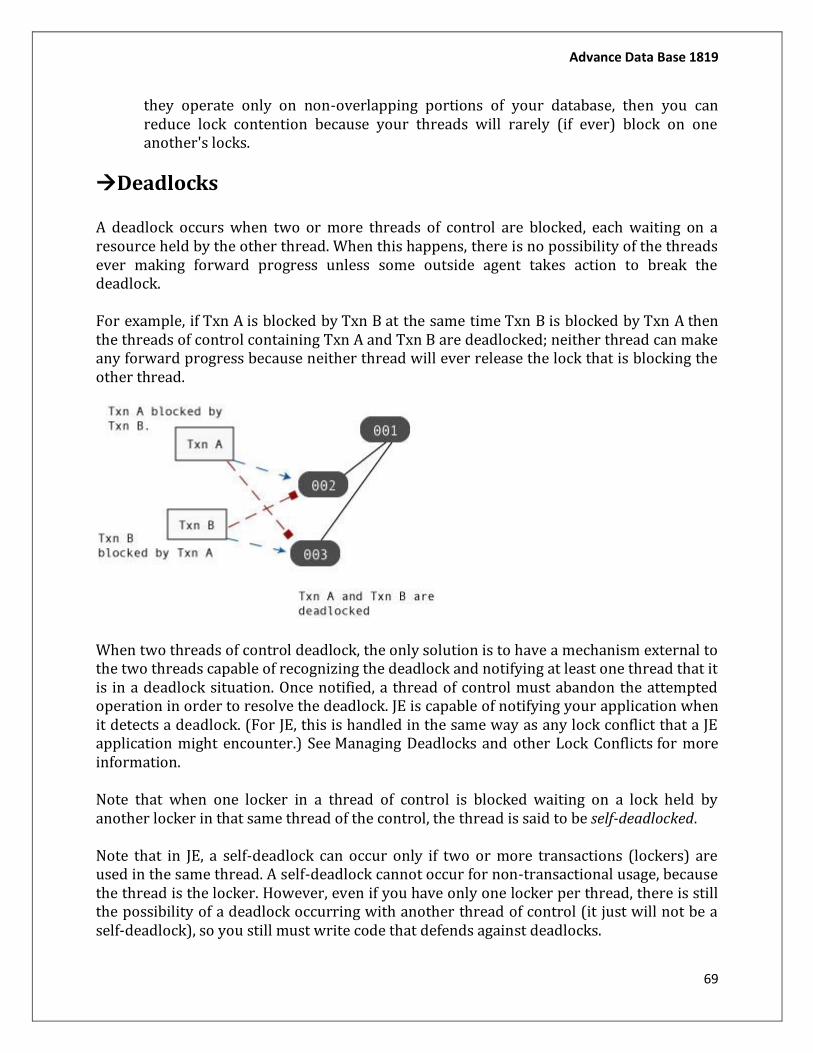
Advance Data Base 1819
69
they operate only on non-overlapping portions of your database, then you can reduce lock contention because your threads will rarely (if ever) block on one another's locks.
Deadlocks
A deadlock occurs when two or more threads of control are blocked, each waiting on a resource held by the other thread. When this happens, there is no possibility of the threads ever making forward progress unless some outside agent takes action to break the deadlock.
For example, if Txn A is blocked by Txn B at the same time Txn B is blocked by Txn A then the threads of control containing Txn A and Txn B are deadlocked; neither thread can make any forward progress because neither thread will ever release the lock that is blocking the other thread.
When two threads of control deadlock, the only solution is to have a mechanism external to the two threads capable of recognizing the deadlock and notifying at least one thread that it is in a deadlock situation. Once notified, a thread of control must abandon the attempted operation in order to resolve the deadlock. JE is capable of notifying your application when it detects a deadlock. (For JE, this is handled in the same way as any lock conflict that a JE application might encounter.) See Managing Deadlocks and other Lock Conflicts for more information.
Note that when one locker in a thread of control is blocked waiting on a lock held by another locker in that same thread of the control, the thread is said to be self-deadlocked.
Note that in JE, a self-deadlock can occur only if two or more transactions (lockers) are used in the same thread. A self-deadlock cannot occur for non-transactional usage, because the thread is the locker. However, even if you have only one locker per thread, there is still the possibility of a deadlock occurring with another thread of control (it just will not be a self-deadlock), so you still must write code that defends against deadlocks.
Advance Data Base 1819
70
Deadlock Avoidance
The things that you do to avoid lock contention also help to reduce deadlocks (see Avoiding Blocks).Beyond that, you should also make sure all threads access data in the same order as all other threads. So long as threads lock records in the same basic order, there is no possibility of a deadlock (threads can still block, however).
Be aware that if you are using secondary databases (indexes), then locking order is different for reading and writing. For this reason, if you are writing a concurrent application and you are using secondary databases, you should expect deadlocks.
Concurrency control:
In information technology and computer science, especially in the fields of computer
programming, operating systems, multiprocessors, and databases, concurrency control
ensures that correct results for concurrent operations are generated, while getting those
results as quickly as possible.
Computer systems, both software and hardware, consist of modules, or components. Each
component is designed to operate correctly, i.e., to obey or to meet certain consistency
rules. When components that operate concurrently interact by messaging or by sharing
accessed data (in memory or storage), a certain component's consistency may be violated
by another component. The general area of concurrency control provides rules, methods,
design methodologies, and theories to maintain the consistency of components operating
concurrently while interacting, and thus the consistency and correctness of the whole
system. Introducing concurrency control into a system means applying operation
constraints which typically result in some performance reduction. Operation consistency
and correctness should be achieved with as good as possible efficiency, without reducing
performance below reasonable levels. Concurrency control can require significant
additional complexity and overhead in a concurrent algorithm compared to the simpler
sequential algorithm.
For example, a failure in concurrency control can result in data corruption from torn read
or write operations.
Concurrency control theory has two classifications for the methods of instituting
concurrency control:
Pessimistic concurrency control
A system of locks prevents users from modifying data in a way that affects other users.
After a user performs an action that causes a lock to be applied, other users cannot perform
actions that would conflict with the lock until the owner releases it. This is called
Advance Data Base 1819
71
pessimistic control because it is mainly used in environments where there is high
contention for data, where the cost of protecting data with locks is less than the cost of
rolling back transactions if concurrency conflicts occur.
Optimistic concurrency control
In optimistic concurrency control, users do not lock data when they read it. When a user
updates data, the system checks to see if another user changed the data after it was read. If
another user updated the data, an error is raised. Typically, the user receiving the error
rolls back the transaction and starts over. This is called optimistic because it is mainly used
in environments where there is low contention for data, and where the cost of occasionally
rolling back a transaction is lower than the cost of locking data when read.
Serializability:
In concurrency control of databases, transaction processing (transaction management),
and various transactional applications (e.g., transactional memory and software
transactional memory), both centralized and distributed, a transaction schedule is
serializable if its outcome (e.g., the resulting database state) is equal to the outcome of its
transactions executed serially, i.e., sequentially without overlapping in time. Transactions
are normally executed concurrently (they overlap), since this is the most efficient way.
Serializability is the major correctness criterion for concurrent transactions' executions. It
is considered the highest level of isolation between transactions, and plays an essential role
in concurrency control. As such it is supported in all general purpose database systems.
Strong strict two-phase locking (SS2PL) is a popular serializability mechanism utilized in
most of the database systems (in various variants) since their early days in the 1970s.
Serializability theory provides the formal framework to reason about and analyze
serializability and its techniques. Though it is mathematical in nature, its fundamentals are
informally (without Mathematics notation) introduced below.
- Serializability is a property of a transaction schedule (history). It relates to
the isolation property of a database transaction.
Serializability of a schedule means equivalence (in the outcome, the database state, data values) to a serial schedule (i.e., sequential with no transaction overlap in time) with the same transactions. It is the major criterion for the correctness of concurrent transactions' schedule, and thus supported in all general purpose database systems.
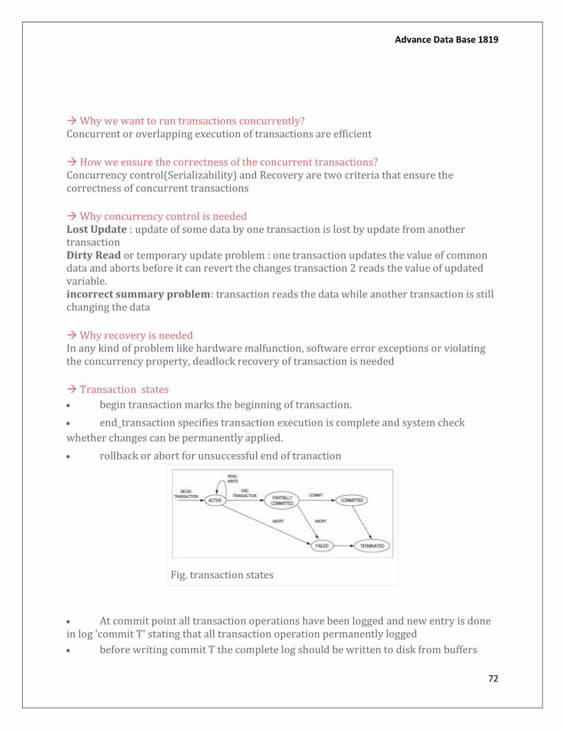
Advance Data Base 1819
72
Why we want to run transactions concurrently? Concurrent or overlapping execution of transactions are efficient
How we ensure the correctness of the concurrent transactions? Concurrency control(Serializability) and Recovery are two criteria that ensure the correctness of concurrent transactions
Why concurrency control is needed Lost Update : update of some data by one transaction is lost by update from another transaction Dirty Read or temporary update problem : one transaction updates the value of common data and aborts before it can revert the changes transaction 2 reads the value of updated variable. incorrect summary problem: transaction reads the data while another transaction is still changing the data
Why recovery is needed In any kind of problem like hardware malfunction, software error exceptions or violating the concurrency property, deadlock recovery of transaction is needed
Transaction states
begin transaction marks the beginning of transaction.
end_transaction specifies transaction execution is complete and system check
whether changes can be permanently applied.
rollback or abort for unsuccessful end of tranaction
Fig. transaction states
At commit point all transaction operations have been logged and new entry is done in log 'commit T' stating that all transaction operation permanently logged
before writing commit T the complete log should be written to disk from buffers
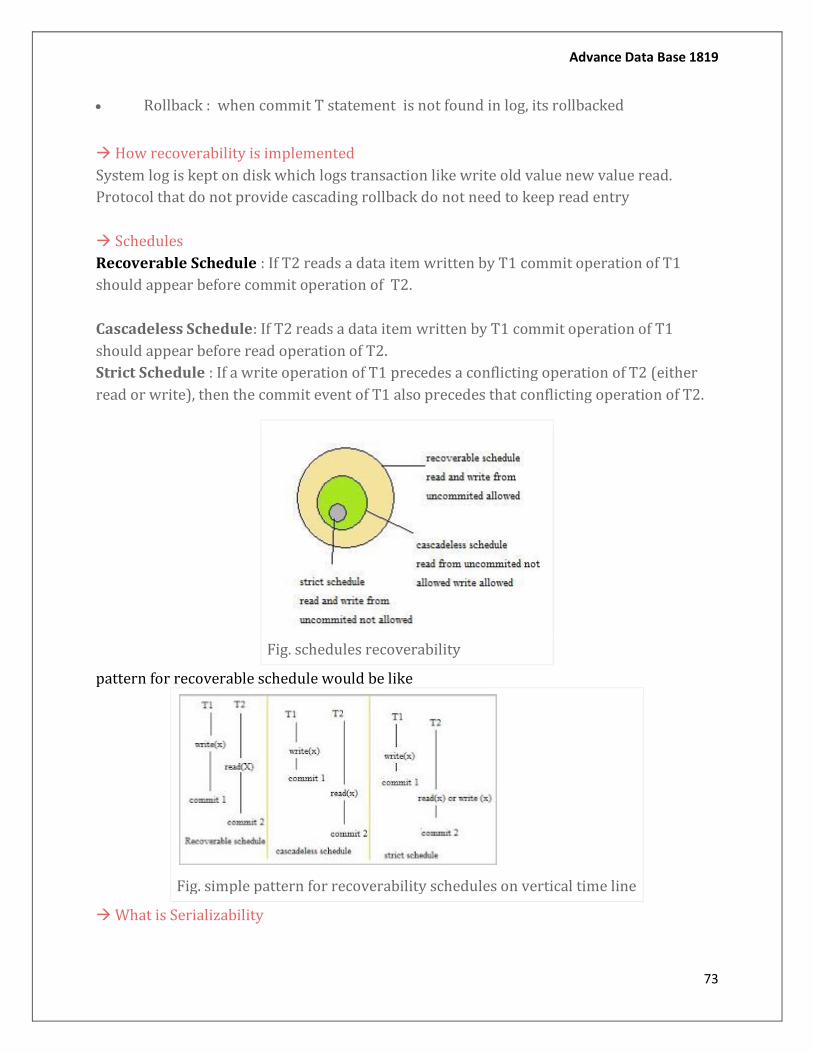
Advance Data Base 1819
73
Rollback : when commit T statement is not found in log, its rollbacked
How recoverability is implemented
System log is kept on disk which logs transaction like write old value new value read.
Protocol that do not provide cascading rollback do not need to keep read entry
Schedules
Recoverable Schedule : If T2 reads a data item written by T1 commit operation of T1
should appear before commit operation of T2.
Cascadeless Schedule: If T2 reads a data item written by T1 commit operation of T1
should appear before read operation of T2.
Strict Schedule : If a write operation of T1 precedes a conflicting operation of T2 (either
read or write), then the commit event of T1 also precedes that conflicting operation of T2.
Fig. schedules recoverability
pattern for recoverable schedule would be like
Fig. simple pattern for recoverability schedules on vertical time line
What is Serializability
Advance Data Base 1819
74
If executing interleaved transaction results in same outcome as serial schedule(running
transaction in some sequnence) then they are considered serializable. this schedule is type
of nonserial schedule.
Types of serializability View and conflict serializability conflict is subset of view serializability
Conflict is widely utilized because it is easier to determine and covers a substantial portion of the view serializable
Equivalence to serial schedule such that
In view serializable, two schedules write and read the same data values.
and In conflict seriablizable, same set of respective chronologically ordered pairs of
conflicting operations.
Conflict serializable
In conflict serializabability two schedules are conflict equivalent and we can reorder the
non conflicting operation to get the serial schedule
Conflicting operation
1) they are upon same data item
2)At least one of them is write
3) they are from different transactions
Non commutative that is their orders matter
DB Locking
DBMS is often criticized for excessive locking – resulting in poor database performance when sharing data among multiple concurrent processes. Is this criticism justified, or is DBMS being unfairly blamed for application design and implementation shortfalls? To evaluate this question, we need to understand more about DBMS locking protocols. In this article, we examine how, why, what and when DBMS locks and unlocks database resources. Future articles will address how to minimize the impact of database locking. THE NEED FOR LOCKING In an ideal concurrent environment, many processes can simultaneously access data in a DBMS database, each having the appearance that they have exclusive access to the database. In practice, this environment is closely approximated by careful use of locking protocols.
Advance Data Base 1819
75
Locking is necessary in a concurrent environment to assure that one process does not retrieve or update a record that is being updated by another process. Failure to use some controls (locking), would result in inconsistent and corrupt data. In addition to record locking, DBMS implements several other locking mechanisms to ensure the integrity of other data structures that provide shared I/O, communication among different processes in a cluster and automatic recovery in the event of a process or cluster failure. While these other lock structures use additional VMS lock resources, they rarely hinder database concurrency, but can actually improve database performance. HOW DBMS USES LOCKS DBMS makes extensive use of the VMS Distributed Lock Manager for controlling virtually every aspect of database access. Use of the Distributed Lock Manager ensures cluster-wide control of database resources, thus allowing DBMS to take advantage of OpenVMS' clustering technology. VMS locks consume system resources. A typical process, running a DBMS application may lock hundreds or thousands of records and database pages at a time. Using a VMS lock for each of these resources in a busy database could easily exhaust these resources. The system parameters: LOCKIDTBL, LOCKIDTBL_MAX, and REHASHTBL parameters determine the number of locks that exist on the system at any one time. To minimize the number of VMS locks required to maintain record and page integrity, DBMS implements a technique called adjustable locking granularity. This allows DBMS to manage a group of resources (pages or records) using a single VMS lock. When a conflicting request is made for the same resource group, the process that is holding the lock is notified that it is blocking another process and automatically reduces the locking-level of the larger group. Adjustable page locking is mandatory and hidden from the database administrator, while adjustable recordlocking can be enabled and tuned or disabled for each database. When adjustable record locking is enabled, DBMS attempts to minimize the number of VMS locks required to maintain database integrity without impacting database concurrency. TYPES OF LOCKS DBMS employs many types of locks to ensure database integrity in a concurrent environment. By using various lock types for different functions, DBMS can provide optimal performance in many different environments.
- Area Locks DBMS uses area locks to implement the DML (Data Manipulation Language) READY statement. If a realm is readied by another run unit, later READY usage modes by other run-units must be compatible with all existing READY usage modes. Area locks can significantly affect database concurrency – however, their impact is only felt during a DML READY statement. Lock conflicts for area locks occur only when you attempt
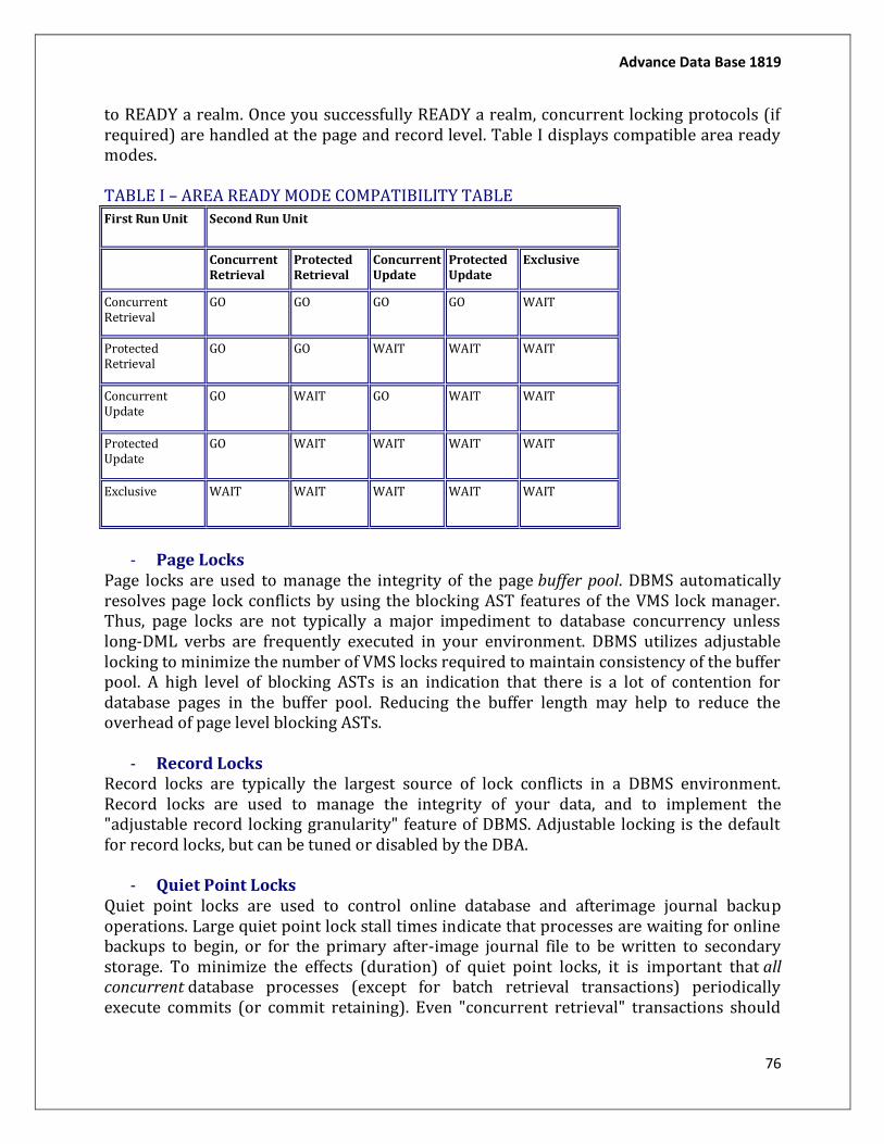
Advance Data Base 1819
76
to READY a realm. Once you successfully READY a realm, concurrent locking protocols (if required) are handled at the page and record level. Table I displays compatible area ready modes. TABLE I – AREA READY MODE COMPATIBILITY TABLE
First Run Unit Second Run Unit
00 Concurrent Retrieval
Protected Retrieval
Concurrent Update
Protected Update
Exclusive
Concurrent Retrieval
GO GO GO GO WAIT
Protected Retrieval
GO GO WAIT WAIT WAIT
Concurrent Update
GO WAIT GO WAIT WAIT
Protected Update
GO WAIT WAIT WAIT WAIT
Exclusive WAIT WAIT WAIT WAIT WAIT
- Page Locks
Page locks are used to manage the integrity of the page buffer pool. DBMS automatically resolves page lock conflicts by using the blocking AST features of the VMS lock manager. Thus, page locks are not typically a major impediment to database concurrency unless long-DML verbs are frequently executed in your environment. DBMS utilizes adjustable locking to minimize the number of VMS locks required to maintain consistency of the buffer pool. A high level of blocking ASTs is an indication that there is a lot of contention for database pages in the buffer pool. Reducing the buffer length may help to reduce the overhead of page level blocking ASTs.
- Record Locks Record locks are typically the largest source of lock conflicts in a DBMS environment. Record locks are used to manage the integrity of your data, and to implement the "adjustable record locking granularity" feature of DBMS. Adjustable locking is the default for record locks, but can be tuned or disabled by the DBA.
- Quiet Point Locks Quiet point locks are used to control online database and afterimage journal backup operations. Large quiet point lock stall times indicate that processes are waiting for online backups to begin, or for the primary after-image journal file to be written to secondary storage. To minimize the effects (duration) of quiet point locks, it is important that all concurrent database processes (except for batch retrieval transactions) periodically execute commits (or commit retaining). Even "concurrent retrieval" transactions should
Advance Data Base 1819
77
periodically "commit [retaining]" their transactions. This ensures that the online backups will achieve a "quiet point" quickly and allow new transactions to proceed.
- Freeze Locks Freeze locks are used to stop (freeze) database activity during database process recovery. When a process terminates abnormally (as a result of a process or node failure, STOP/ID, or a CTRL-Y/STOP), all locks held by that process are automatically released. If transactions were allowed to continue, database corruption would result. Thus, when a process terminates abnormally, DBMS uses the freeze lock to stop database activity until the failed process(es) can be recovered. Freeze locks typically are not a major source of contention in most environments. However, if you are subject to frequent system or process failures, or users are using CTRL-Y/STOP to exit from programs, freeze locks could hinder database concurrency.
- DATABASE QUALIFIERS Several of the DBMS creation and modification qualifiers have a direct impact on database locking characteristics. Establishing the appropriate mix of qualifiers in your environment can help minimize the impact of database locking.
- /HOLD_RETRIEVAL_LOCKS The [no]hold_retrieval_locks qualifier, determines whether DBMS holds read-only record locks on all records read for the duration of the transaction (until the next COMMIT [without the RETAINING option] or ROLLBACK). Holding retrieval locks guarantees that any records previously read during a transaction willnot have been changed by another run-unit during the same transaction. While this increases theconsistency of your transaction, it can significantly degrade concurrency. This option should only be used if your transactions read very few records and consistency of all records read must be guaranteed throughout the transaction. By default, DBMS uses /NOHOLD_RETRIEVAL_LOCKS. The logical name, DBM$BIND_HOLD_RETRIEVAL_LOCKS may be used to override the default established in the root file. If DBM$BIND_HOLD_RETRIEVAL_LOCKS translates to "1" then all records read by the transaction are locked until the end of the transaction. Software Concepts International recommends against using hold retrieval locks in most environments.
- /[NO]WAIT_RECORD_LOCKS The [no]wait_record_locks qualifier determines whether a run-unit waits when requesting a record that islocked in a conflicting mode by another run-unit or if it receives a "lock conflict" exception. This qualifieronly determines if the requesting run-unit will receive a "lock conflict" exception – not a "deadlock"exception (deadlock exceptions are always returned when they occur). When the default (WAIT_RECORD_LOCKS) is used, DBMS will not generate a "lock conflict" exception, and the blocked process will continue to wait until the record is unlocked. Thus, the process can continue to wait indefinitely until the record is unlocked by the other run-unit. The logical name, DBM$BIND_WAIT_RECORD_LOCKS may be used to override the default established in the root file. Again, a value of "1" enables wait on record lock conflicts, and a
Advance Data Base 1819
78
value of "0" causes the process to receive the "lock conflict" exception. Software Concepts International recommends clients to WAIT on record conflicts. This allows the application to trap for "deadlocks," and avoids "live-lock" situations that cannot be detected. In addition, the wait on record conflicts can be used with the /TIMEOUT to give the application control over records locked for an excessive duration.
- /TIMEOUT=LOCK=seconds The timeout qualifier allows you to specify the amount of time that a run-unit waits for a locked record before returning a "lock timeout" exception. This qualifier must be used with the "wait" on record locks (above). The logical name, DBM$BIND_LOCK_TIMEOUT_INTERVAL may be used to override the default established in the root file. The value of the translation determines the number of seconds to wait for a locked record. If your applications trap the ‘DBM$TIMEOUT’ exceptions, then Software Concepts International recommends using lock timeouts with a time of at least 60 seconds. Using the /TIMEOUT qualifier only if your application is designed to handle "lock timeout" exceptions. COBOL shops that use declaratives, may want to handle "DBM$_DEADLOCK", "DBM$LCKCNFLCT", and "DBM$TIMEOUT" exceptions in the same "USE" section.
- /ADJUSTABLE_LOCKING Enabling, disabling, or modifying the values of the adjustable locking features of DBMS will not significantly reduce record lock conflicts. However, adjustable locking can significantly affect the amount of lock resources your application uses, as well as the overall overhead associated with record locking. The DBO/SHOW STATISTICS (record locking) screen provides useful insights into the potential benefits and costs of adjustable locking. If you observe a blocking AST rate that is more than 20-25% of the number of locks requested plus locks promoted, then this may indicate significant adjustable locking overhead. In this case, try disabling adjustable locking, or reducing the number of levels in its tree.
- /[NO]LOCK_OPTIMIZATION Lock optimization sounds so obvious. Who wouldn't want "lock optimization?" Lock optimization (the default) only controls whether area locks are held from one transaction to another. This avoids the overhead of acquiring and releasing locks for each transaction. In environments where long DML verbs are frequently executed, lock optimization may actually degrade performance. This is because the process holding the lock does not release the NOWAIT lock until the end of its current DML verb. Thus, if the current DML verb takes a long time to complete, the process trying to ready the realm may experience a long delay.
- /SNAPSHOTS=(option) Snapshots are included in this discussion of locking, because the use of snapshots (batch retrieval transactions) can significantly reduce the level of lock contention in your database. Although snapshot transactions are subject to page and other resource lock conflicts, they are never involved in record lock conflicts – thus providing significantly increased concurrency between read-only and update transactions.

Advance Data Base 1819
79
Enabling snapshots are not however a panacea – All update processes (except EXCLUSIVE or BATCH) must write before-images of their updates to the snapshot files. The use of /DEFERRED qualifier minimizes this affect by allowing update processes to write to the snapshot file only when snapshot transactions are active.
- BUFFER COUNT Additional or excessive buffers require additional page level locking to manage the buffer pool. If you are using large buffer counts, you may need to increase the enque limits on your processes, as well as the SYSGEN parameters, LOCKIDTBL, LOCKIDTBL_MAX and REHASHTBL.
- DBMS LOCK EXCEPTIONS DBMS signals one of three types of exceptions when a process encounters a locked record – a deadlock, a lock conflict or a lock timeout.
- Deadlocks Exceptions A deadlock exception, DBM$_DEADLOCK, is returned when two run-units attempt to access a resource in mutually exclusive modes, and each run-unit is waiting for a resource that the other run-unit holds. This indicates that neither run-unit can continue unless one of the run-units releases its locks. When a deadlock occurs, DBMS will choose a "victim," and signal that run-unit of the deadlock condition. This does not cause the "victim" to automatically release its locks. The victim process should immediately execute a 'rollback' to release its locks.
- Lock Conflict Exceptions DBMS will only return the lock conflict exception, DBM$_LCKCNFLCT, when the run-unit is bound to a database with "/NOWAIT_RECORD_LOCKS" enabled and it attempts to access a record that is locked in a mutually exclusive mode by another run-unit. Note, that only the "blocked" run-unit receives the exception.
- Lock Timeout Exceptions The third type of exception is the lock timeout exception, DBM$TIMEOUT. A lock timeout only occurs when the "/TIMEOUT=LOCK=nnn" and "/NOWAIT_RECORD_LOCKS" are enabled and a run-unit attempts to access a record that is locked in a mutually exclusive mode by another run-unit.
Specialized Locking Techniques
A static view of a database has been considered for locking as discussed so far. In reality, a
database is dynamic since the size of database changes over time. To deal with the dynamic
nature of database, we need some specialized locking techniques, which are discussed in
this section.
Advance Data Base 1819
80
10.3.1. Handling the Phantom Problem
Due to the dynamic nature of database, the phantom problem may arise. Consider
the BOOK relation of Online Book database that stores information about books including
their price. Now, suppose that the PUBLISHER relation is modified to store information
about average price of books that are published by corresponding publishers in the
attribute Avg_price. Consider a transaction T1 that verifies whether the average price of
books in PUBLISHER relation for the publisher P001 is consistent with the information
about the individual books recorded in BOOKrelation that are published by P001. T1 first
locks all the tuples of books that are published by P001 in BOOK relation and thereafter
locks the tuple in PUBLISHER relation referring to P001. Meanwhile, another
transaction T2 inserts a new tuple for a book published by P001 into BOOKrelation, and
then, before T1 locks the tuple in PUBLISHER relation referring to P001, T2 locks this tuple
and updates it with the new value. In this case, average information of T1 will be
inconsistent even though both transactions follow two-phase locking, since new book tuple
is not taken into account. The new book tuple inserted into BOOK relation by T2 is called
a phantom tuple. This is because T1 assumes that the relation it has locked includes all
information of books published by P001, and this assumption is violated when T2 inserted
the new book tuple into BOOK relation.
Performance of Locking
Normally, two factors govern the performance of locking, namely, resource
contention and data contention. Resource contention refers to the contention over
memory space, computing time and other resources. It determines the rate at which a
transaction executes between its lock requests. On the other hand, data contention refers
to the contention over data. It determines the number of currently executing transactions.
Now, assume that the concurrency control is turned off; in that case the transactions suffer
from resource contention. For high loads, the system may thrash, that is, the throughput of
the system first increases and then decreases. Initially, the throughput increases since only
few transactions request the resources. Later, with the increase in the number of
transactions, the throughput decreases. If the system has enough resources (memory
space, computing power, etc.) that make the contention over resources negligible, the
transactions only suffer from data contention. For high loads, the system may thrash due
to aborting (or rollback) and blocking. Both the mechanisms degrade the performance.
Timestamp-Based Technique
So far, we have discussed that the locks with the two-phase locking ensures the
serializability of schedules. Two-phase locking generates the serializable schedules based
Advance Data Base 1819
81
on the order in which the transactions acquire the locks on the data items. A transaction
requesting a lock on a locked data item may be forced to wait till the data item is unlocked.
Serializability of the schedules can also be ensured by another method, which involves
ordering the execution of the transactions in advance using timestamps.
Timestamp-based concurrency control is a non-lock concurrency control
technique, hence, deadlocks cannot occur.
Optimistic (or Validation) Technique
All the concurrency control techniques, discussed so far (locking and timestamp ordering)
result either in transaction delay or transaction rollback, thereby named as pessimistic
techniques. These techniques require performing a check before executing any read or
write operation. For instance, in locking, a check is done to determine whether the data
item being accessed is locked. On the other hand, in timestamp ordering, a check is done on
the timestamp of the transaction against the read and write timestamps of the data item to
determine whether the transaction can access the data item. These checks can be expensive
and represent overhead during transaction execution as they slow down the transactions.
In addition, these checks are unnecessary overhead when a majority of transactions are
read-only transactions. This is because the rate of conflicts among these transactions may
be low. Therefore, these transactions can be executed without applying checks and still
maintaining the consistency of the system by using an alternative technique, known
as optimistic (or validation) technique.
Concurrency control and locking
The purpose of concurrency control is to prevent two different users (or two different
connections by the same user) from trying to update the same data at the same time.
Concurrency control can also prevent one user from seeing out-of-date data while another
user is updating the same data.
The following examples explain why concurrency control is needed. For both examples,
suppose that your checking account contains $1,000. During the day you deposit $300 and
spend $200 from that account. At the end of the day your account should have $1,100.
Example 1: No concurrency control
At 11:00 AM, bank teller #1 looks up your account and sees that you have $1,000. The teller
subtracts the $200 check, but is not able to save the updated account balance ($800)
immediately.
Advance Data Base 1819
82
At 11:01 AM, another teller #2 looks up your account and still sees the $1,000 balance.
Teller #2 then adds your $300 deposit and saves your new account balance as $1,300.
At 11:09 AM, bank teller #1 returns to the terminal, finishes entering and saving the
updated value that is calculated to be $800. That $800 value writes over the $1300.
At the end of the day, your account has $800 when it should have had $1,100 ($1000 + 300
- 200).
Example 2: Concurrency control
When teller #1 starts working on your account, a lock is placed on the account.
When teller #2 tries to read or update your account while teller #1 is updating your
account, teller #2 will not be given access and gets an error message.
After teller #1 has finished the update, teller #2 can proceed.
At the end of the day, your account has $1,100 ($1000 - 200 + 300).
In Example 1, the account updates are done simultaneously rather than in sequence and
one update write overwrites another update. In Example 2, to prevent two users from
updating the data simultaneously (and potentially writing over each other's updates), the
system uses a concurrency control mechanism.
solidDB® offers two different concurrency control mechanisms, pessimistic concurrency
control and optimistic concurrency control.
The pessimistic concurrency control mechanism is based on locking. A lock is a mechanism
for limiting other users' access to a piece of data. When one user has a lock on a record, the
lock prevents other users from changing (and in some cases reading) that record.
Optimistic concurrency control mechanism does not place locks but prevents the
overwriting of data by using timestamps.
Crash Recovery
Though we are living in highly technologically advanced era where hundreds of satellite monitor the earth and at every second billions of people are connected through information technology, failure is expected but not every time acceptable.
DBMS is highly complex system with hundreds of transactions being executed every second. Availability of DBMS depends on its complex architecture and underlying hardware or system software. If it fails or crashes amid transactions being executed, it is expected
Advance Data Base 1819
83
that the system would follow some sort of algorithm or techniques to recover from crashes or failures.
Failure Classification
To see where the problem has occurred we generalize the failure into various categories, as follows:
TRANSACTION FAILURE
When a transaction is failed to execute or it reaches a point after which it cannot be completed successfully it has to abort. This is called transaction failure. Where only few transaction or process are hurt.
Reason for transaction failure could be:
Logical errors: where a transaction cannot complete because of it has some code error or any internal error condition
System errors: where the database system itself terminates an active transaction because DBMS is not able to execute it or it has to stop because of some system condition. For example, in case of deadlock or resource unavailability systems aborts an active transaction.
SYSTEM CRASH
There are problems, which are external to the system, which may cause the system to stop abruptly and cause the system to crash. For example interruption in power supply, failure of underlying hardware or software failure.
Examples may include operating system errors.
DISK FAILURE:
In early days of technology evolution, it was a common problem where hard disk drives or storage drives used to fail frequently.
Disk failures include formation of bad sectors, unreachability to the disk, disk head crash or any other failure, which destroys all or part of disk storage
Storage Structure
We have already described storage system here. In brief, the storage structure can be divided in various categories:
Volatile storage: As name suggests, this storage does not survive system crashes and mostly placed very closed to CPU by embedding them onto the chipset itself for examples: main memory, cache memory. They are fast but can store a small amount of information.

Advance Data Base 1819
84
Nonvolatile storage: These memories are made to survive system crashes. They are huge in data storage capacity but slower in accessibility. Examples may include, hard disks, magnetic tapes, flash memory, non-volatile (battery backed up) RAM.
Recovery and Atomicity
When a system crashes, it many have several transactions being executed and various files opened for them to modifying data items. As we know that transactions are made of various operations, which are atomic in nature. But according to ACID properties of DBMS, atomicity of transactions as a whole must be maintained that is, either all operations are executed or none.
When DBMS recovers from a crash it should maintain the following:
It should check the states of all transactions, which were being executed.
A transaction may be in the middle of some operation; DBMS must ensure the atomicity of transaction in this case.
It should check whether the transaction can be completed now or needs to be rolled back.
No transactions would be allowed to left DBMS in inconsistent state.
There are two types of techniques, which can help DBMS in recovering as well as maintaining the atomicity of transaction:
Maintaining the logs of each transaction, and writing them onto some stable storage before actually modifying the database.
Maintaining shadow paging, where are the changes are done on a volatile memory and later the actual database is updated.
Log-Based Recovery
Log is a sequence of records, which maintains the records of actions performed by a transaction. It is important that the logs are written prior to actual modification and stored on a stable storage media, which is failsafe.
Log based recovery works as follows:
The log file is kept on stable storage media
When a transaction enters the system and starts execution, it writes a log about it
<Tn, Start>
When the transaction modifies an item X, it write logs as follows:
Advance Data Base 1819
85
<Tn, X, V1, V2>
It reads Tn has changed the value of X, from V1 to V2.
When transaction finishes, it logs:
<Tn, commit>
Database can be modified using two approaches:
1. Deferred database modification: All logs are written on to the stable storage and database is updated when transaction commits.
2. Immediate database modification: Each log follows an actual database modification. That is, database is modified immediately after every operation.
Recovery with concurrent transactions
When more than one transactions are being executed in parallel, the logs are interleaved. At the time of recovery it would become hard for recovery system to backtrack all logs, and then start recovering. To ease this situation most modern DBMS use the concept of 'checkpoints'.
CHECKPOINT
Keeping and maintaining logs in real time and in real environment may fill out all the memory space available in the system. At time passes log file may be too big to be handled at all. Checkpoint is a mechanism where all the previous logs are removed from the system and stored permanently in storage disk. Checkpoint declares a point before which the DBMS was in consistent state and all the transactions were committed.
RECOVERY
When system with concurrent transaction crashes and recovers, it does behave in the following manner:
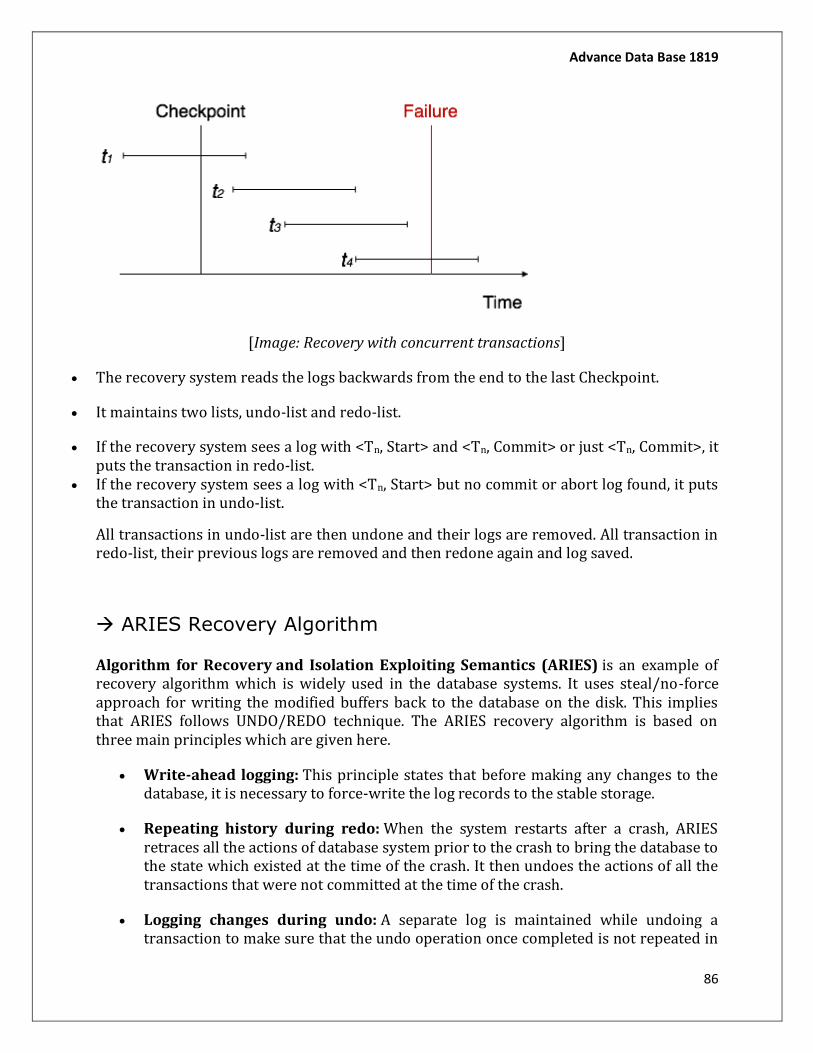
Advance Data Base 1819
86
[Image: Recovery with concurrent transactions]
The recovery system reads the logs backwards from the end to the last Checkpoint.
It maintains two lists, undo-list and redo-list.
If the recovery system sees a log with <Tn, Start> and <Tn, Commit> or just <Tn, Commit>, it puts the transaction in redo-list.
If the recovery system sees a log with <Tn, Start> but no commit or abort log found, it puts the transaction in undo-list.
All transactions in undo-list are then undone and their logs are removed. All transaction in redo-list, their previous logs are removed and then redone again and log saved.
ARIES Recovery Algorithm
Algorithm for Recovery and Isolation Exploiting Semantics (ARIES) is an example of recovery algorithm which is widely used in the database systems. It uses steal/no-force approach for writing the modified buffers back to the database on the disk. This implies that ARIES follows UNDO/REDO technique. The ARIES recovery algorithm is based on three main principles which are given here.
Write-ahead logging: This principle states that before making any changes to the database, it is necessary to force-write the log records to the stable storage.
Repeating history during redo: When the system restarts after a crash, ARIES retraces all the actions of database system prior to the crash to bring the database to the state which existed at the time of the crash. It then undoes the actions of all the transactions that were not committed at the time of the crash.
Logging changes during undo: A separate log is maintained while undoing a transaction to make sure that the undo operation once completed is not repeated in

Advance Data Base 1819
87
case the failure occurs during the recovery itself, which causes restart of the recovery process.
ARIES Recovery
ARIES (Algorithm for Recovery and Isolation Exploiting Semantics) recovery is based on
the Write Ahead Logging (WAL) protocol. Every update operation writes a log record
which is one of
An undo-only log record: Only the before image is logged. Thus, an undo operation can be
done to retrieve the old data.
A redo-only log record: Only the after image is logged. Thus, a redo operation can be
attempted.
An undo-redo log record. Both before image and after images are logged.
Every log record is assigned a unique and monotonically increasing log sequence number
(LSN). Every data page has a page LSN field that is set to the LSN of the log record
corresponding to the last update on the page. WAL requires that the log record
corresponding to an update make it to stable storagegif before the data page corresponding
to that update is written to disk. For performance reasons, each log write is not
immediately forced to disk. A log tail is maintained in main memory to buffer log writes.
The log tail is flushed to disk when it gets full. A transaction cannot be declared committed
until the commit log record makes it to disk.
Once in a while the recovery subsystem writes a checkpoint record to the log. The
checkpoint record contains the transaction table (which gives the list of active
transactions) and the dirty page table (the list of data pages in the buffer pool that have not
yet made it to disk). A master log record is maintained separately, in stable storage, to store
the LSN of the latest checkpoint record that made it to disk. On restart, the recovery
subsystem reads the master log record to find the checkpoint's LSN, reads the checkpoint
record, and starts recovery from there on.
The actual recovery process consists of three passes:
Analysis. The recovery subsystem determines the earliest log record from which the next
pass must start. It also scans the log forward from the checkpoint record to construct a
snapshot of what the system looked like at the instant of the crash.
Redo. Starting at the earliest LSN determined in pass (1) above, the log is read forward and
each update redone.
Advance Data Base 1819
88
Undo. The log is scanned backward and updates corresponding to loser transactions are
undone.
For further details of the recovery process, see [Mohan et al. 92,Ramamurthy & Tsoi 95].
It is clear from this description of ARIES that the following features are required for a log
manager:
Ability to write log records. The log manager should maintain a log tail in main memory
and write log records to it. The log tail should be written to stable storage on demand or
when the log tail gets full. Implicit in this requirement is the fact that the log tail can
become full halfway through the writing of a log record. It also means that a log record can
be longer than a pagegif.
Ability to wraparound. The log is typically maintained on a separate disk. When the log
reaches the end of the disk, it is wrapped around back to the beginning.
Ability to store and retrieve the master log record. The master log record is stored
separately in stable storage, possibly on a different duplex-disk.
Ability to read log records given an LSN. Also, the ability to scan the log forward from a
given LSN to the end of log. Implicit in this requirement is that the log manager should be
able to detect the end of the log and distinguish the end of the log from a valid log record's
beginning.
Ability to create a log. In actual practice, this will require setting up a duplex-disk for the
log, a duplex-disk for the master log record, and a raw device interface to read and write
the disks bypassing the Operating System.
Ability to maintain the log tail. This requires some sort of shared memory because the
log tail is common to all transactions accessing the database the log corresponds to. Mutual
exclusion of log writes and reads have to be taken care of.
The following sections describe some simplifying assumptions that we have made to fit the
protocol into Minirel and the interface and implementation of our log manager.
Write-ahead logging:
In computer science, write-ahead logging (WAL) is a family of techniques for
providing atomicity and durability (two of the ACID properties) in database
systems.
Advance Data Base 1819
89
In a system using WAL, all modifications are written to a log before they are
applied. Usually both redo and undo information is stored in the log.
The purpose of this can be illustrated by an example. Imagine a program that
is in the middle of performing some operation when the machine it is running
on loses power. Upon restart, that program might well need to know whether
the operation it was performing succeeded, half-succeeded, or failed. If a
write-ahead log were used, the program could check this log and compare
what it was supposed to be doing when it unexpectedly lost power to what
was actually done. On the basis of this comparison, the program could decide
to undo what it had started, complete what it had started, or keep things as
they are.
WAL allows updates of a database to be done in-place. Another way to
implement atomic updates is with shadow paging, which is not in-place. The
main advantage of doing updates in-place is that it reduces the need to modify
indexes and block lists.
ARIES is a popular algorithm in the WAL family.
File systems typically use a variant of WAL for at least file system metadata
called journaling.
The PostgreSQL database system also uses WAL to provide point-in-time
recovery and database replication features.
SQLite database also uses WAL.
MongoDB uses write-ahead logging to provide consistency and crash safety.
Apache HBase uses WAL in order to provide recovery after disaster.
Write-Ahead Logging (WAL)
The Write-Ahead Logging Protocol:
Must force the log record for an update before the
corresponding data page gets to disk.
Must write all log records for a Xact before commit.
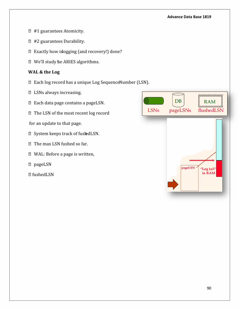
Advance Data Base 1819
90
#1 guarantees Atomicity.
#2 guarantees Durability.
Exactly how is logging (and recovery!) done?
We’ll study the ARIES algorithms.
WAL & the Log
Each log record has a unique Log Sequence Number (LSN).
LSNs always increasing.
Each data page contains a pageLSN.
The LSN of the most recent log record
for an update to that page.
System keeps track of fushedLSN.
The max LSN fushed so far.
WAL: Before a page is written,
pageLSN
fushedLSN
Advance Data Base 1819
91
UNIT-4
Database Storage:-
Databases are stored physically as files of records on some storage medium. This section
will deal with the overview of avaiable storage media then briefly describes the magnetic
storage devices.
Physical Storage Media:The collection of data in a database system must be stored
physically on some storage medium. These storage media are classified by the speed with
which data can be accessed, by the cost per unit of data to buy the medium and by the
medium’s reliability. There are several typical storage media available:
Cache memory: Cache memory is a primary storage media like the main memory. Data on
these devices can be directly processed by the Central Processing Unit (CPU). Cache
memory is the fastest but is also the most expensive form of storage.
Main memory: Data that are available to be operated are stored in main memory. The
machines instructions operate on main memory. Main memory is lower cost and also lower
speed in compare with cache memory. However, main memory is generally too small to
store the entire database. Main memory is volatile that means contents of main memory
are lost in case of power outage.
Flash memory : This memory is non-volatile and has fast access speed. However, the
drawback of this is the complication when writing data to flash memory. Data in flash
memory cannot be over written directly. To overwrite memory that has been written
already, we have to erase an entire block of memory at once, it is then ready to be written
again.
Magnetic-disk storage: This is the primary medium for long-term storage of data. This is a
type of secondary storages which usually have large capacity, cost less and volatile. Data in
secondary storage such as magnetic disk cannot be access directly by CPU, first it must be
copied into primary storage.
Optical storage: The most popular optical storage is CD-ROM. In this device data are
stored optically and are read by laser. CD-ROMs contains prerecorded data that cannot be
overwritten. Optical storages are gigabytes in capacity and last much longer than magnetic
disk. Optical jukebox memories use an arrays of CD-ROM platters which are loaded onto
drives on demand.
Tape storage: This storage is used for backup and archival data. Although magnetic tape is
much cheaper than disks. access to data is much slower because taple must be accessed
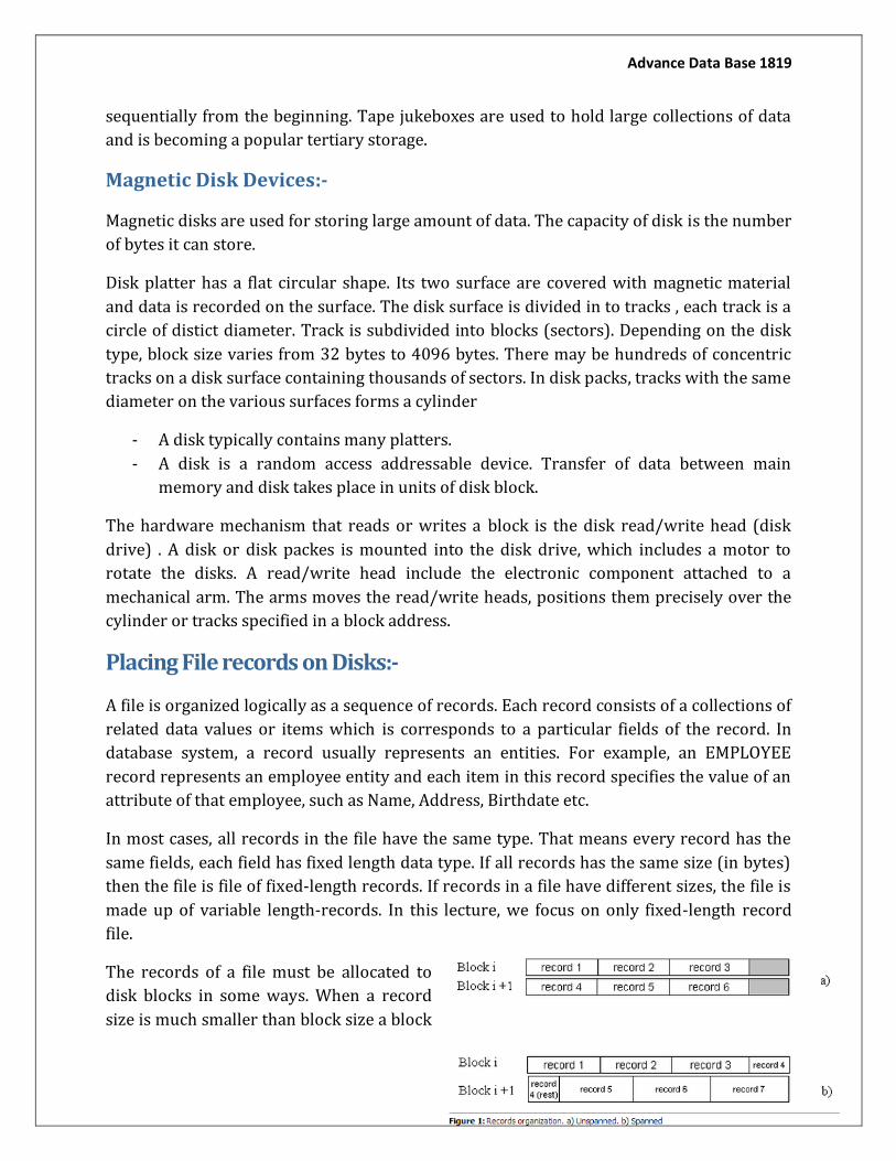
Advance Data Base 1819
92
sequentially from the beginning. Tape jukeboxes are used to hold large collections of data
and is becoming a popular tertiary storage.
Magnetic Disk Devices:-
Magnetic disks are used for storing large amount of data. The capacity of disk is the number
of bytes it can store.
Disk platter has a flat circular shape. Its two surface are covered with magnetic material
and data is recorded on the surface. The disk surface is divided in to tracks , each track is a
circle of distict diameter. Track is subdivided into blocks (sectors). Depending on the disk
type, block size varies from 32 bytes to 4096 bytes. There may be hundreds of concentric
tracks on a disk surface containing thousands of sectors. In disk packs, tracks with the same
diameter on the various surfaces forms a cylinder
- A disk typically contains many platters.
- A disk is a random access addressable device. Transfer of data between main
memory and disk takes place in units of disk block.
The hardware mechanism that reads or writes a block is the disk read/write head (disk
drive) . A disk or disk packes is mounted into the disk drive, which includes a motor to
rotate the disks. A read/write head include the electronic component attached to a
mechanical arm. The arms moves the read/write heads, positions them precisely over the
cylinder or tracks specified in a block address.
Placing File records on Disks:-
A file is organized logically as a sequence of records. Each record consists of a collections of
related data values or items which is corresponds to a particular fields of the record. In
database system, a record usually represents an entities. For example, an EMPLOYEE
record represents an employee entity and each item in this record specifies the value of an
attribute of that employee, such as Name, Address, Birthdate etc.
In most cases, all records in the file have the same type. That means every record has the
same fields, each field has fixed length data type. If all records has the same size (in bytes)
then the file is file of fixed-length records. If records in a file have different sizes, the file is
made up of variable length-records. In this lecture, we focus on only fixed-length record
file.
The records of a file must be allocated to
disk blocks in some ways. When a record
size is much smaller than block size a block
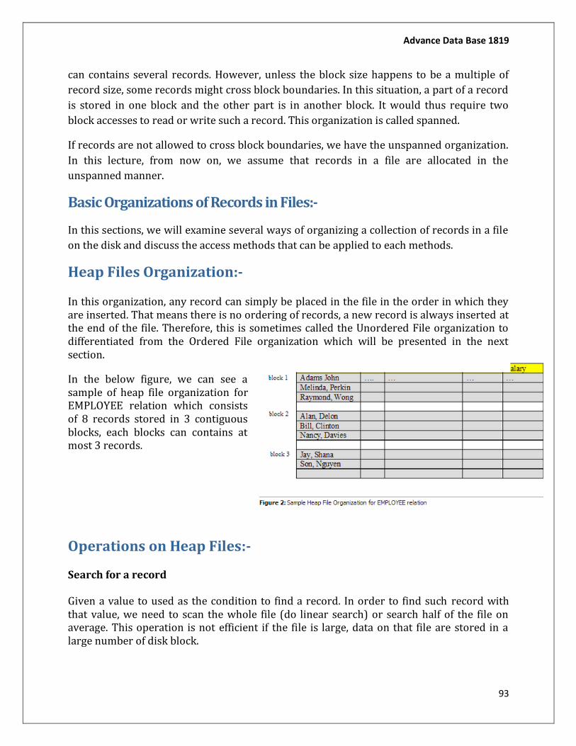
Advance Data Base 1819
93
can contains several records. However, unless the block size happens to be a multiple of
record size, some records might cross block boundaries. In this situation, a part of a record
is stored in one block and the other part is in another block. It would thus require two
block accesses to read or write such a record. This organization is called spanned.
If records are not allowed to cross block boundaries, we have the unspanned organization.
In this lecture, from now on, we assume that records in a file are allocated in the
unspanned manner.
Basic Organizations of Records in Files:-
In this sections, we will examine several ways of organizing a collection of records in a file
on the disk and discuss the access methods that can be applied to each methods.
Heap Files Organization:-
In this organization, any record can simply be placed in the file in the order in which they are inserted. That means there is no ordering of records, a new record is always inserted at the end of the file. Therefore, this is sometimes called the Unordered File organization to differentiated from the Ordered File organization which will be presented in the next section.
In the below figure, we can see a sample of heap file organization for EMPLOYEE relation which consists of 8 records stored in 3 contiguous blocks, each blocks can contains at most 3 records.
Operations on Heap Files:-
Search for a record
Given a value to used as the condition to find a record. In order to find such record with that value, we need to scan the whole file (do linear search) or search half of the file on average. This operation is not efficient if the file is large, data on that file are stored in a large number of disk block.
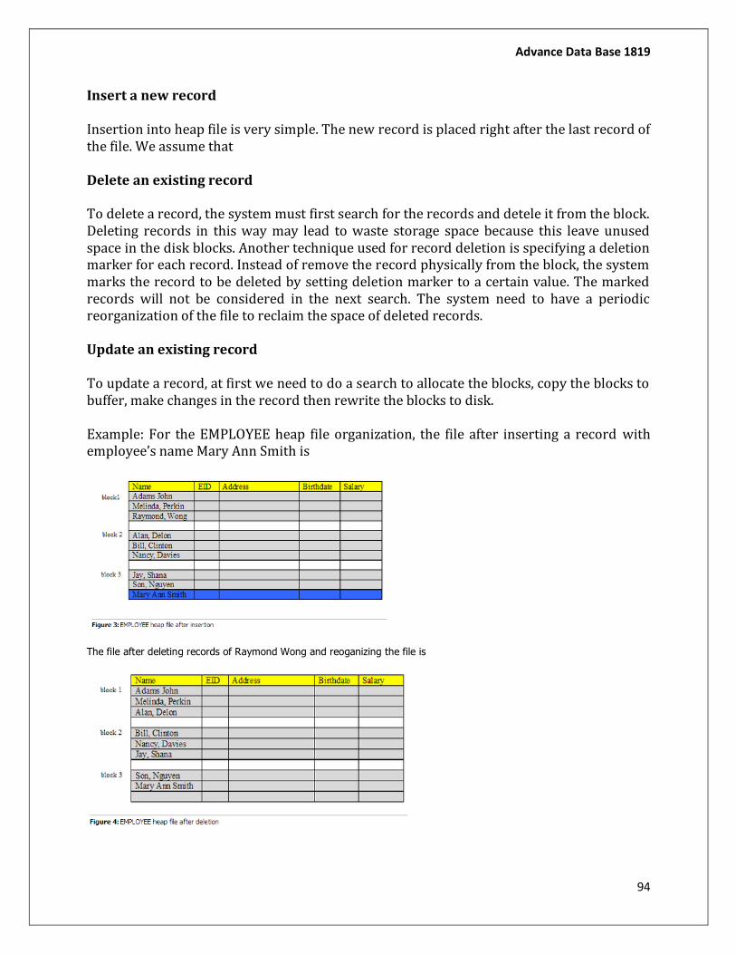
Advance Data Base 1819
94
Insert a new record
Insertion into heap file is very simple. The new record is placed right after the last record of the file. We assume that
Delete an existing record
To delete a record, the system must first search for the records and detele it from the block. Deleting records in this way may lead to waste storage space because this leave unused space in the disk blocks. Another technique used for record deletion is specifying a deletion marker for each record. Instead of remove the record physically from the block, the system marks the record to be deleted by setting deletion marker to a certain value. The marked records will not be considered in the next search. The system need to have a periodic reorganization of the file to reclaim the space of deleted records.
Update an existing record
To update a record, at first we need to do a search to allocate the blocks, copy the blocks to buffer, make changes in the record then rewrite the blocks to disk.
Example: For the EMPLOYEE heap file organization, the file after inserting a record with employee’s name Mary Ann Smith is
The file after deleting records of Raymond Wong and reoganizing the file is
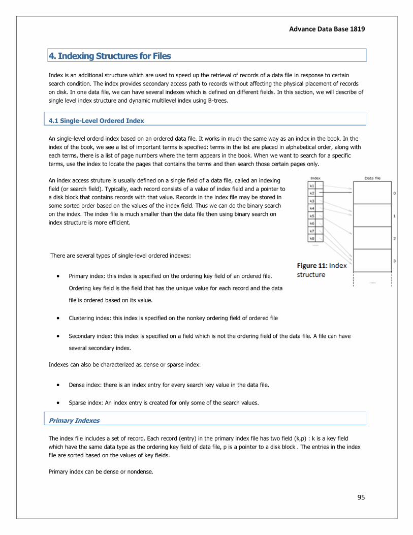
Advance Data Base 1819
95
4. Indexing Structures for Files
Index is an additional structure which are used to speed up the retrieval of records of a data file in response to certain
search condition. The index provides secondary access path to records without affecting the physical placement of records
on disk. In one data file, we can have several indexes which is defined on different fields. In this section, we will describe of
single level index structure and dynamic multilevel index using B-trees.
4.1 Single-Level Ordered Index
An single-level orderd index based on an ordered data file. It works in much the same way as an index in the book. In the
index of the book, we see a list of important terms is specified: terms in the list are placed in alphabetical order, along with
each terms, there is a list of page numbers where the term appears in the book. When we want to search for a specific
terms, use the index to locate the pages that contains the terms and then search those certain pages only.
An index access struture is usually defined on a single field of a data file, called an indexing
field (or search field). Typically, each record consists of a value of index field and a pointer to
a disk block that contains records with that value. Records in the index file may be stored in
some sorted order based on the values of the index field. Thus we can do the binary search
on the index. The index file is much smaller than the data file then using binary search on
index structure is more efficient.
There are several types of single-level ordered indexes:
Primary index: this index is specified on the ordering key field of an ordered file.
Ordering key field is the field that has the unique value for each record and the data
file is ordered based on its value.
Clustering index: this index is specified on the nonkey ordering field of ordered file
Secondary index: this index is specified on a field which is not the ordering field of the data file. A file can have
several secondary index.
Indexes can also be characterized as dense or sparse index:
Dense index: there is an index entry for every search key value in the data file.
Sparse index: An index entry is created for only some of the search values.
Primary Indexes
The index file includes a set of record. Each record (entry) in the primary index file has two field (k,p) : k is a key field
which have the same data type as the ordering key field of data file, p is a pointer to a disk block . The entries in the index
file are sorted based on the values of key fields.
Primary index can be dense or nondense.
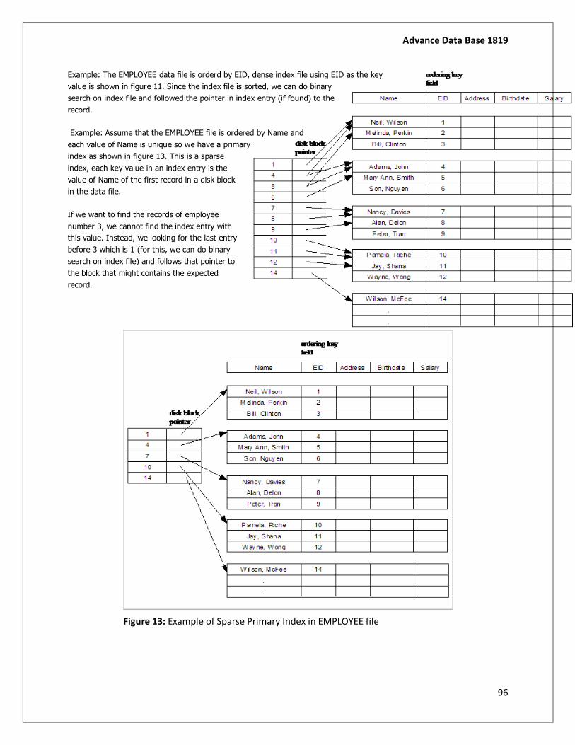
Advance Data Base 1819
96
Example: The EMPLOYEE data file is orderd by EID, dense index file using EID as the key
value is shown in figure 11. Since the index file is sorted, we can do binary
search on index file and followed the pointer in index entry (if found) to the
record.
Example: Assume that the EMPLOYEE file is ordered by Name and
each value of Name is unique so we have a primary
index as shown in figure 13. This is a sparse
index, each key value in an index entry is the
value of Name of the first record in a disk block
in the data file.
If we want to find the records of employee
number 3, we cannot find the index entry with
this value. Instead, we looking for the last entry
before 3 which is 1 (for this, we can do binary
search on index file) and follows that pointer to
the block that might contains the expected
record.
Figure 13: Example of Sparse Primary Index in EMPLOYEE file
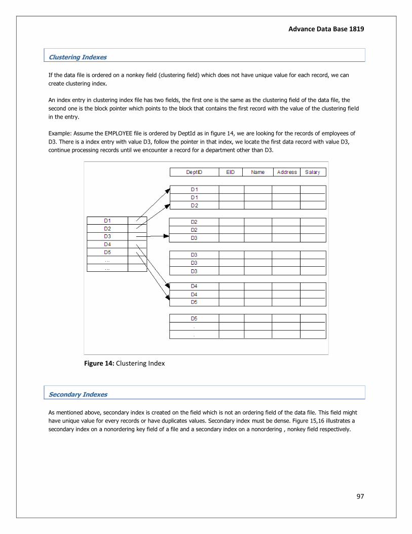
Advance Data Base 1819
97
Clustering Indexes
If the data file is ordered on a nonkey field (clustering field) which does not have unique value for each record, we can
create clustering index.
An index entry in clustering index file has two fields, the first one is the same as the clustering field of the data file, the
second one is the block pointer which points to the block that contains the first record with the value of the clustering field
in the entry.
Example: Assume the EMPLOYEE file is ordered by DeptId as in figure 14, we are looking for the records of employees of
D3. There is a index entry with value D3, follow the pointer in that index, we locate the first data record with value D3,
continue processing records until we encounter a record for a department other than D3.
Figure 14: Clustering Index
Secondary Indexes
As mentioned above, secondary index is created on the field which is not an ordering field of the data file. This field might
have unique value for every records or have duplicates values. Secondary index must be dense. Figure 15,16 illustrates a
secondary index on a nonordering key field of a file and a secondary index on a nonordering , nonkey field respectively.
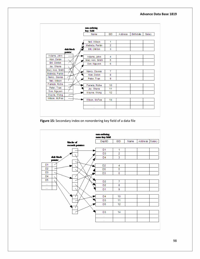
Advance Data Base 1819
98
Figure 15: Secondary index on nonordering key field of a data file
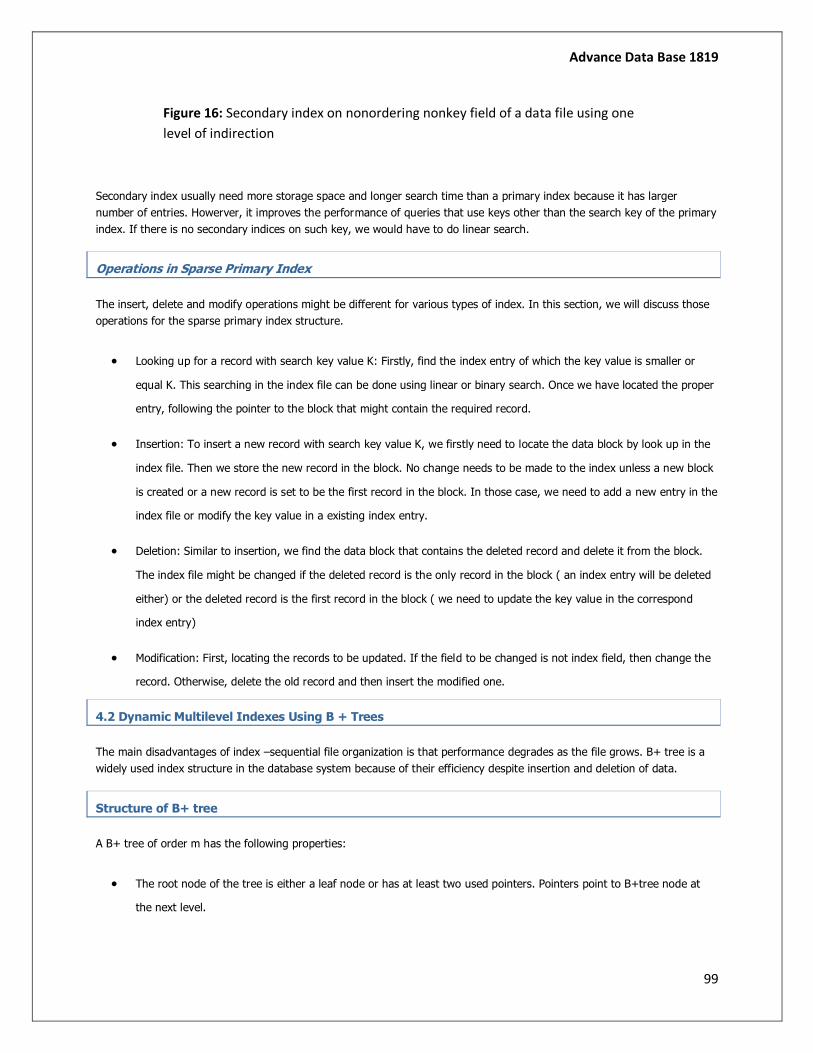
Advance Data Base 1819
99
Figure 16: Secondary index on nonordering nonkey field of a data file using one
level of indirection
Secondary index usually need more storage space and longer search time than a primary index because it has larger
number of entries. Howerver, it improves the performance of queries that use keys other than the search key of the primary
index. If there is no secondary indices on such key, we would have to do linear search.
Operations in Sparse Primary Index
The insert, delete and modify operations might be different for various types of index. In this section, we will discuss those
operations for the sparse primary index structure.
Looking up for a record with search key value K: Firstly, find the index entry of which the key value is smaller or
equal K. This searching in the index file can be done using linear or binary search. Once we have located the proper
entry, following the pointer to the block that might contain the required record.
Insertion: To insert a new record with search key value K, we firstly need to locate the data block by look up in the
index file. Then we store the new record in the block. No change needs to be made to the index unless a new block
is created or a new record is set to be the first record in the block. In those case, we need to add a new entry in the
index file or modify the key value in a existing index entry.
Deletion: Similar to insertion, we find the data block that contains the deleted record and delete it from the block.
The index file might be changed if the deleted record is the only record in the block ( an index entry will be deleted
either) or the deleted record is the first record in the block ( we need to update the key value in the correspond
index entry)
Modification: First, locating the records to be updated. If the field to be changed is not index field, then change the
record. Otherwise, delete the old record and then insert the modified one.
4.2 Dynamic Multilevel Indexes Using B + Trees
The main disadvantages of index –sequential file organization is that performance degrades as the file grows. B+ tree is a
widely used index structure in the database system because of their efficiency despite insertion and deletion of data.
Structure of B+ tree
A B+ tree of order m has the following properties:
The root node of the tree is either a leaf node or has at least two used pointers. Pointers point to B+tree node at
the next level.

Advance Data Base 1819
100
The leaf node in B+ tree have an entry for every values of the search field along with a data pointer to the record
(or to a block that contains this record). The last pointer points to the next leaf to the right. A leaf node contains at
least ⌊m/2⌋ and at most m-1 values. Leaf node is of the form (<k1, p1>, <k2, p2>, …,<km-1, pm-1>, pm)
where pm is the pointer to the next node.
Each internal node in B+ tree is of the form (p1, k1, p2, k2, …, pm-1, km-1, pm). It contains up to m-1 search key
values k1, k2, k3, …, km-1 and m pointers p1, p2, p3, … pm. The search key values within a node is sorted k1 < k2
< k3 <…< km-1. Actually, the internal nodes in B+ tree forms multilevel sparse index on the leaf nodes. At
least ⌈m/2⌉pointers in the internal node are used.
All paths from root node to leaf nodes have equal length.
Figure 17: Example of B+ tree with order 4
Searching for a record with search key value k with B+ tree
Searching for the record with search key value k in a tree B means we need to find the path from root node to a leaf node
that might contains values k.
If the root of B is leaf node, look among the search key values there. If the values is found in position i then pointer
i is the pointer to the desire record.
If we are at a internal node with key values k1, k2, k3, …, km-1, we examine the node, looking for the smallest
search key value greater than k. Assume that this search key value is ki , we follow the pointer pi the the node in
the next level. If k < k1 then follows p1, if we have m pointers in the node and k >= km-1 then we follows pm the
the node in next level. Recursively apply the search procedure at the node in next level
Inserting a record with search key value k in a B+ tree of order m
Using searching to find the leaf node L to store new pair <key, pointer> to the new record.
If there is enough space for the new pair in L, put the pair there.
If there is no room in L, we split L into two leaf nodes and divide the keys between two leaf node so each is at least
half full.
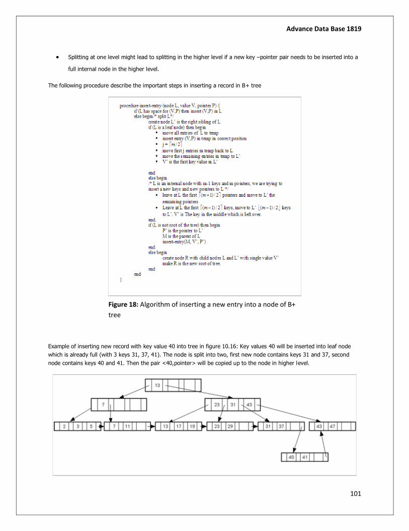
Advance Data Base 1819
101
Splitting at one level might lead to splitting in the higher level if a new key –pointer pair needs to be inserted into a
full internal node in the higher level.
The following procedure describe the important steps in inserting a record in B+ tree
Figure 18: Algorithm of inserting a new entry into a node of B+
tree
Example of inserting new record with key value 40 into tree in figure 10.16: Key values 40 will be inserted into leaf node
which is already full (with 3 keys 31, 37, 41). The node is split into two, first new node contains keys 31 and 37, second
node contains keys 40 and 41. Then the pair <40,pointer> will be copied up to the node in higher level.
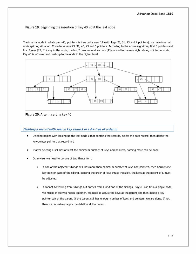
Advance Data Base 1819
102
Figure 19: Beginning the insertion of key 40, split the leaf node
The internal node in which pair<40, pointer> is inserted is also full (with keys 23, 31, 43 and 4 pointers), we have internal
node splitting situation. Consider 4 keys 23, 31, 40, 43 and 5 pointers. According to the above algorithm, first 3 pointers and
first 2 keys (23, 31) stay in the node, the last 2 pointers and last key (43) moved to the new right sibling of internal node.
Key 40 is left over and push up to the node in the higher level.
Figure 20: After inserting key 40
Deleting a record with search key value k in a B+ tree of order m
Deleting begins with looking up the leaf node L that contains the records, delete the data record, then delete the
key-pointer pair to that record in L
If after deleting L still has at least the minimum number of keys and pointers, nothing more can be done.
Otherwise, we need to do one of two things for L
If one of the adjacent siblings of L has more than minimum number of keys and pointers, then borrow one
key-pointer pairs of the sibling, keeping the order of keys intact. Possibly, the keys at the parent of L must
be adjusted.
If cannot borrowing from siblings but entries from L and one of the siblings , says L’ can fit in a single node,
we merge these two nodes together. We need to adjust the keys at the parent and then delete a key-
pointer pair at the parent. If the parent still has enough number of keys and pointers, we are done. If not,
then we recursively apply the deletion at the parent.
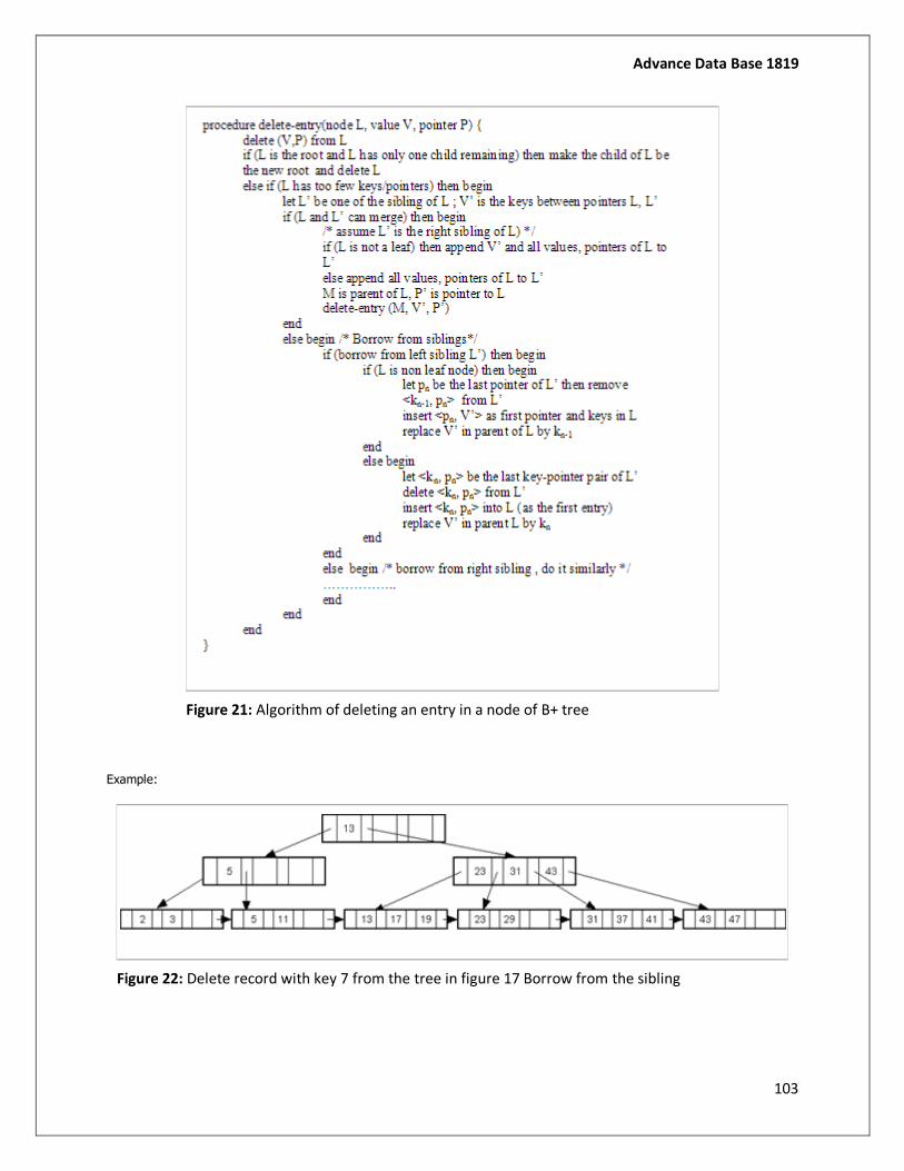
Advance Data Base 1819
103
Figure 21: Algorithm of deleting an entry in a node of B+ tree
Example:
Figure 22: Delete record with key 7 from the tree in figure 17 Borrow from the sibling
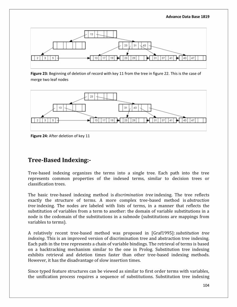
Advance Data Base 1819
104
Figure 23: Beginning of deletion of record with key 11 from the tree in figure 22. This is the case of
merge two leaf nodes
Figure 24: After deletion of key 11
Tree-Based Indexing:-
Tree-based indexing organizes the terms into a single tree. Each path into the tree represents common properties of the indexed terms, similar to decision trees or classification trees.
The basic tree-based indexing method is discrimination tree indexing. The tree reflects exactly the structure of terms. A more complex tree-based method is abstraction tree indexing. The nodes are labeled with lists of terms, in a manner that reflects the substitution of variables from a term to another: the domain of variable substitutions in a node is the codomain of the substitutions in a subnode (substitutions are mappings from variables to terms).
A relatively recent tree-based method was proposed in [Graf1995]: substitution tree indexing. This is an improved version of discrimination tree and abstraction tree indexing. Each path in the tree represents a chain of variable bindings. The retrieval of terms is based on a backtracking mechanism similar to the one in Prolog. Substitution tree indexing exhibits retrieval and deletion times faster than other tree-based indexing methods. However, it has the disadvantage of slow insertion times.
Since typed feature structures can be viewed as similar to first order terms with variables, the unification process requires a sequence of substitutions. Substitution tree indexing
Advance Data Base 1819
105
could be applied to TFSGs; unfortunately, published experimental results [Graf1995] indicating slow insertion times suggest that a method performing more efficient operations during run time is to be preferred. Future work will investigate possible adaptations of this technique to TFSG parsing.
Indexing in Database Systems
Although database systems are not in the scope of this thesis, many of the techniques developed here are connected to the database area. Since the subject of indexing in databases is very vast, just a few essential bibliographical pointers are mentioned in this section.
Databases can store large amounts of data. Usually, each stored entity is a complex structure, called a record (similar to a feature structure). Records are indexed based on the values of certain fields (features). The retrieval is usually not limited to a query where specific values are requested for a field, but must support other types of queries (such as interval queries - where the values should belong to a given interval). An interesting research topic in the area of indexing are the self-adaptive indexing methods, where the indexing can be (semi-)automatically configured. One of the first published work on this topic is [Hammer and Chan1976].
Most of the available database textbooks (such as [Elmasri and Navathe2000]) have chapters dedicated to indexing. Recent research papers on indexing can be found in Kluwer Academic Publishers' series ``Advances in Database Systems'': [Bertino et al.1997], [Manolopoulos et al.1999], or [Mueck and Polaschek1997].
A major difference between indexing in databases and indexing in a TFSG parser should be noted. Typically, a database consists of a large collection of objects, and the indexing scheme is designed to improve retrieval times. It is expected that databases are persistent, with fewer deletions and insertions than retrievals. From this point of view, parsing can be seen as managing a volatile database, that is always empty at start-up. The ratio between insertions and retrievals in a database application is very small (even equal to 0 when used only to retrieve data). For indexed parsing, this ratio is much higher and depends on the structure of grammar rules. For this reason (similar to those discussed in Section 5.2.3), indexing methods such as B-trees (commonly used in databases), where the retrieval can
be performed in operations, but the insertion needs operations
Storing Data: Disks and Files
Advance Data Base 1819
106
Low Level Data Storage
Because a database generally stores huge amounts of data, a database engine
pays careful attention to most low-level aspects of memory management. The
memory management policies are key to a DBMS, for reasons of efficiency,
portability and overall control. Therefore, most comercial operating systems take
care to implement policies which would otherwise be handled by the Operating
System.
Memory Hierarchy
The typical memory hierarchy has multiple layers. A relatively simple example of
such a hierarchy is the following:
CPU | CACHE | MAIN MEMORY | MAGNETIC DISK | TAPE ARCHIVE
We will focus most of our attention on the interactions between neighboring
levels of this hierarchy, and particular between main memory and the magnetic
disk.
Data is predominantly stored on the magnetic disk, for several reasons:
The amount of data stored in a typical database can not be expected to
fit in main memory.
An individual file may be so large that they could not be fully addressed
by a 32-bit computer, even if it could reside in main memory.
For crash recovery, much of the data must be stored using non-volatile
memory, and the disk drive generally serves this purpose.
At the same time, for the CPU to operate on any piece of data, that data must first
be brought into main memory, if not already there. Because the access time to
read/write a block of data from/to disk is orders of magnitude longer than most
CPU operations, the number of disk I/O's is generally the bottleneck in terms of
efficiency for database operations.
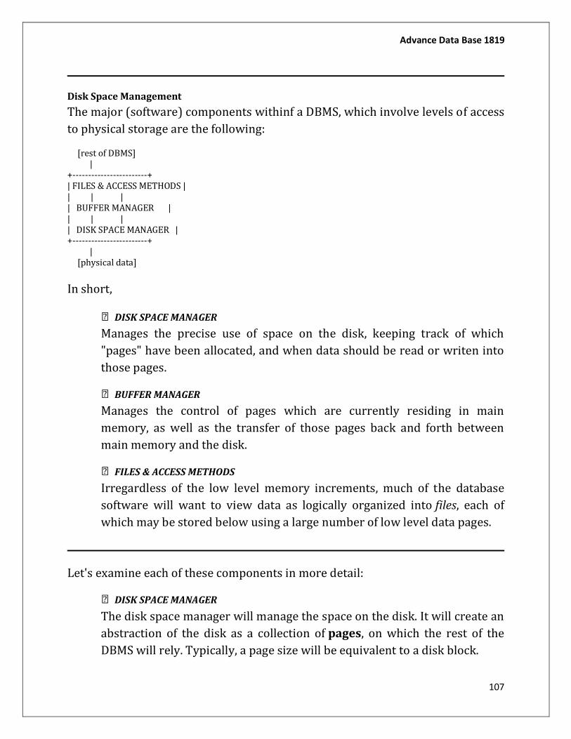
Advance Data Base 1819
107
Disk Space Management
The major (software) components withinf a DBMS, which involve levels of access
to physical storage are the following:
[rest of DBMS] | +------------------------+ | FILES & ACCESS METHODS | | | | | BUFFER MANAGER | | | | | DISK SPACE MANAGER | +------------------------+ | [physical data]
In short,
DISK SPACE MANAGER
Manages the precise use of space on the disk, keeping track of which
"pages" have been allocated, and when data should be read or writen into
those pages.
BUFFER MANAGER
Manages the control of pages which are currently residing in main
memory, as well as the transfer of those pages back and forth between
main memory and the disk.
FILES & ACCESS METHODS
Irregardless of the low level memory increments, much of the database
software will want to view data as logically organized into files, each of
which may be stored below using a large number of low level data pages.
Let's examine each of these components in more detail:
DISK SPACE MANAGER
The disk space manager will manage the space on the disk. It will create an
abstraction of the disk as a collection of pages, on which the rest of the
DBMS will rely. Typically, a page size will be equivalent to a disk block.
Advance Data Base 1819
108
Typical operations which it will support are:
Reading a page of data from the disk
Writing a page of data to the disk
Allocating or Deallocating a page of the disk for use
possibly allocating a group of "consecutive" pages for use
To manage the disk space, it must keep track of all of the current free blocks. This is generally done in one of two ways.
via a "free list"
via a "bitmap"
BUFFER MANAGER
The CPU can only operate on data which exists in main memory. The buffer
manager will be responsible for transfering pages between the main
memory and the underlying disk.
The buffer manager organizes main memory into a collection of frames, where each frame has the ability to hold one page. The overall collection of these frames is refered to as the buffer pool. When a higher-level portion of the DBMS needs access to a page (referenced by a pageID), it will explicitly request that page from the Buffer Manager. Furthermore, that portion of the DBMS is expected to explicitly "release" the page, informing the Buffer Manager when it is no longer needed in main memory for the time being.
When a portion of the DBMS submits a requests to the Buffer Manager for a particular page, the manager must first determine whether or not this page is already in the current buffer pool. Generaly, this can be accomplished by keeping a pair (pageID,frameNum) for each page which is currently in the pool. By storing this information in a hash table, the buffer manager can look up a given pageID, to find if it is already in the pool, and if so, in which frame.
When a requested page is not in the buffer pool, the Buffer Manager will need to send a request to the Disk Manager to read that page from the disk,

Advance Data Base 1819
109
and it will need to determine which frame to store it in, and thus which existing page of the buffer pool to evict.
The decision of which page to evict is complicated by several factors:
Several current processes may have requested a particular page
at the same time, and that page can only be released from memory
after all of the requesting processes have released the page.
To accomplish this, a pin_count is kept for each page currently in the buffer. The count is initially zero; is incremented each time a request for the page is served (a.k.a. "pinning); and is decremented each time a process subsequently releases the page (a.k.a. "unpinning").
Thus, the evicted page must be chosen from those pages with a current pin count of zero. (if no such pages exist, then
There may be several candidate pages for eviction. There are
many factors that might influence our choice; we can adopt a
particular "replacement policy" for such decisions. (we defer the
discussion of such policies for the moment).
When a page is going to be evicted, we must be concerned as to
whether the contents of that page in main memory were altered
since the time it was brought in from the disk. If so, we must make
sure to write the contents of the page back to the disk (via the Disk
Manager). Conversely, if the page was only read, then we can
remove it from main memory, knowing that the contents are still
accurate on disk.
To accomplish this, a boolean value known as the dirty bit is kept for each page in the buffer pool. When read from disk, the dirty bit is initially set to false. However, when each process releases the page, it must also inform the buffer manager of whether or not it had changed any of the memory contents while it was checked out. If so, then the dirty bit is set to true, ensuring that the contents will later be written to disk should this page be evicted.
Buffer Replacement Policies
LRU (Least Recently Used)

Advance Data Base 1819
110
FIFO (First In First Out)
CLOCK
This is meant to have behavior in the style of LRU yet with less
overhead. Associated with each page is a referenced bit.
Whenever the pin count is decremented to zero, the
referenced bit is turned on.
When looking for a page to evict, a counter current is used to scan all candidated pages. When current reaches a page:
If the pin count is non-zero, the current page is left
alone, and the current variable cycles to the next page.
If the pin count is zero, but the referenced bit is on,
then the current page is left alone but the referenced bit
is turned off, after which the current variable cycles to
the next page.
If the pin count is zero and the referenced bit is off,
then this page is evicted.
MRU (Most Recently Used)
RANDOM
Which policy to use depends on the access pattern of the database.
Fortunately, the access pattern is often predictable and so the DBMS
can take advantage of this knowledge.
There are also times where a DBMS needs to be able to force a particular page to be written to the disk immediately, and so the buffer manager must support this type of request.
FILES & ACCESS METHODS
As we work with higher-level portions of the DBMS, we must consider how
data will be stored on the disk. We will consider all data to be represented
as files, each of which is a collection of records. If all of the records of a file
Advance Data Base 1819
111
cannot fit on a single page of the disk, then multiple pages will be used to
represent that file.
For example, for a typical table in a relational database, each tuple would be a record, and the (unordered) set of tuples would be stored in a single file. Of course, other internal data for the DBMS can also be viewed as records and files.
Each record has a unique identifier called a record id (rid). Among other things, this will identify the disk address of the page which contains the record.
The file and access layer will manage the abstraction of a file of records. It will support the creation and destruction of files, as well as the insertion and deletion of records to and from the file. It will also support the retrieval of a particular record identified by rid, or a scan operation to step through all records of the file, one at a atime.
Implementation
The file layer will need to keep track of what pages are being used in a
particular file, as well as how the records of the file are organized on those
pages.
There are several issues to address:
Whether the records in a file are to be maintained as an ordered
collection or unordered.
Whether the records of a given file are of fixed size or of variable
size.
We will consider three major issues:
Format of a single record
Format of a single page
Format of a single file
Advance Data Base 1819
112
Format of a single record
Fixed-Length Records
This is an easy scenario. If each field of record has a fixed-
length, then the underlying data can be stored directly one
field after another. Based on the known structure of the
record, offsets can be calculated for accessing any given field.
Variable-Length Records
If these records represent tuples from a relation, then each
record must have the same number of fields. However, some
domains may be used which result in fields that are variable in
length.
There are two general approaches to handling such records:
Separate fields with a chosen delimiter (control
character). Then, the fields can be identified by
scanning the entire record.
Reserve some space at the beginning of the record to
provide offsets to the start of each field of the record.
This allows you to jump to any particular field of the
record.
The second of these approaches is generally prefered, as it
offers minimal overhead, and gives more efficient access to an
arbitrary field.
In general, working with variable length fields introduces some other subtle complexities:
Modifying a field may cause the record to grow,
which may effect the page's placement of the record.
In fact, a record's growth may mean that it no loner
fits in the space remaining on its current page.
A single record could potentially be so large that that
record does not even fit on a single page by itself.

Advance Data Base 1819
113
Format of a single page
If Fixed-Length Records
Consider the page to be broken into uniform slots, where the slot size is equal to the record size. An rid will be represented as < pageID, slot#>
How to handle insertions and deletions depends on whether such rid's are held externally. If we are allowed to move arbitrarily reorganize records, than we can efficiently ensure that all N records are kept in the first N slots of the page. However, if a record's rid must remain consistent, then we will have to leave "holes" after a deletion, and will have to scan for open slots upon an insertion.
If Variable-Length Records
With variable length records, we can no longer consider the page to be broken into fixed slots, because we do not know what size slots to use. Instead, we will have to devote available space in a page to store a newly inserted record, if possible.
Again, our approach will depend greatly on whether or not we are allowed to rearrange the order and placement of the records, at risk of redefining a record's rid. If we are allowed to adjust the placement of existing records, then we can always ensure that all of the records are kept compactly at one end of the page, and that all remaining freespace is contiguous at the other end of the page.
However, if the validity of rid's must be preserved over time, we must adjust this approach. Our solution will be to add one level of indirection in the rid. Rather than have the rid directly reference the true placement of the record on the page, it can reference an entry in a slot directory maintained on the page, where that entry contains information about the true placement.
Though this change of approach may seem insignificant, it allows us to internally rearrange the placement of the records
Advance Data Base 1819
114
of a page, so long as we update the slot directory in accordance.
One additional subtlety is that we still must manage the use of available entries in the slot directory as insertions and deletions of records take place. An existing page's record ID is now represented as < pageID, slotDirectoryEntry >.
Format of a single file
Linked List of pages
A small bit of space on each page can be used to represent the
links to the previous or following pages in the file.
If desired, the pages of a file can be kept in one of two separate linked lists:
One list contains those pages that are completely full
Another list contains those pages that have some
remaining free space
Of course, this approach will not be very helpful with variable-
length records, because it is quite unlikely that any pages will
be completely full.
In either case, finding an existing page with sufficient space for a new record may require walking through many pages from the list (and thus many I/Os, one per page).
Directory of Pages
Another approach is to separately maintain a directory of
pages (using some additional pages for the directory itself).
The directory can contain an entry for each page of the file,
representing whether that page has any free space or perhaps
how much free space.
To locate a page with enough free space for a new record may still require scanning the directory to find a suitable page. The advantage is that far fewer I/Os will be spent scanning the directory, as many directory entires will fit on a single page.
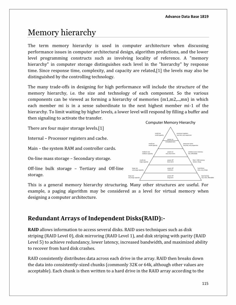
Advance Data Base 1819
115
Memory hierarchy
The term memory hierarchy is used in computer architecture when discussing
performance issues in computer architectural design, algorithm predictions, and the lower
level programming constructs such as involving locality of reference. A "memory
hierarchy" in computer storage distinguishes each level in the "hierarchy" by response
time. Since response time, complexity, and capacity are related,[1] the levels may also be
distinguished by the controlling technology.
The many trade-offs in designing for high performance will include the structure of the
memory hierarchy, i.e. the size and technology of each component. So the various
components can be viewed as forming a hierarchy of memories (m1,m2,...,mn) in which
each member mi is in a sense subordinate to the next highest member mi-1 of the
hierarchy. To limit waiting by higher levels, a lower level will respond by filling a buffer and
then signaling to activate the transfer.
There are four major storage levels.[1]
Internal – Processor registers and cache.
Main – the system RAM and controller cards.
On-line mass storage – Secondary storage.
Off-line bulk storage – Tertiary and Off-line
storage.
This is a general memory hierarchy structuring. Many other structures are useful. For
example, a paging algorithm may be considered as a level for virtual memory when
designing a computer architecture.
Redundant Arrays of Independent Disks(RAID):-
RAID allows information to access several disks. RAID uses techniques such as disk
striping (RAID Level 0), disk mirroring (RAID Level 1), and disk striping with parity (RAID
Level 5) to achieve redundancy, lower latency, increased bandwidth, and maximized ability
to recover from hard disk crashes.
RAID consistently distributes data across each drive in the array. RAID then breaks down
the data into consistently-sized chunks (commonly 32K or 64k, although other values are
acceptable). Each chunk is then written to a hard drive in the RAID array according to the

Advance Data Base 1819
116
RAID level employed. When the data is read, the process is reversed, giving the illusion that
the multiple drives in the array are actually one large drive.
What is RAID?
RAID (redundant array of independent disks; originally redundant array of inexpensive disks) is a way of storing the same data in different places (thus, redundantly) on multiple hard disks. By placing data on multiple disks, I/O (input/output) operations can overlap in a balanced way, improving performance. Since multiple disks increases the mean time between failures (MTBF), storing data redundantly also increases fault tolerance.
Who Should Use RAID?
System Administrators and others who manage
large amounts of data would benefit from using
RAID technology. Primary reasons to deploy RAID
include:
- Enhances speed
- Increases storage capacity using a single
virtual disk
- Minimizes disk failure
Hardware RAID versus Software RAID
There are two possible RAID approaches: Hardware RAID and Software RAID.
Hardware RAID
The hardware-based array manages the RAID subsystem independently from the host. It presents a single disk per RAID array to the host.
A Hardware RAID device connects to the SCSI controller and presents the RAID arrays as a single SCSI drive. An external RAID system moves all RAID handling "intelligence" into a controller located in the external disk subsystem. The whole subsystem is connected to the host via a normal SCSI controller and appears to the host as a single disk.
RAID controller cards function like a SCSI controller to the operating system, and handle all the actual drive communications. The user plugs the drives into the RAID controller (just like a normal SCSI controller) and then adds them to the RAID controllers configuration, and the operating system won't know the difference.
Advance Data Base 1819
117
Software RAID
Software RAID implements the various RAID levels in the kernel disk (block device) code. It offers the cheapest possible solution, as expensive disk controller cards or hot-swap chassis [1] are not required. Software RAID also works with cheaper IDE disks as well as SCSI disks. With today's faster CPUs, Software RAID outperforms Hardware RAID.
The Linux kernel contains an MD driver that allows the RAID solution to be completely hardware independent. The performance of a software-based array depends on the server CPU performance and load.
To learn more about Software RAID, here are the key features:
o Threaded rebuild process o Kernel-based configuration o Portability of arrays between Linux machines without reconstruction o Backgrounded array reconstruction using idle system resources o Hot-swappable drive support o Automatic CPU detection to take advantage of certain CPU optimizations
RAID Standard levels
A number of standard schemes have evolved. These are called levels. Originally, there were
five RAID levels, but many variations have evolved—notably several nested levelsand
many non-standard levels (mostly proprietary). RAID levels and their associated data formats
are standardized by the Storage Networking Industry Association (SNIA) in the Common
RAID Disk Drive Format (DDF) standard:
RAID 0
RAID 0 comprises striping (but neither parity nor mirroring). This level provides no data redundancy nor fault tolerance, but improves performance through parallelism of read and write operations across multiple drives. RAID 0 has no error detection mechanism, so the failure of one disk causes the loss of all data on the array.
RAID 1
RAID 1 comprises mirroring (without parity or striping). Data is written identically to two (or more) drives, thereby producing a "mirrored set". The read request is serviced by any of the drives containing the requested data. This can improve performance if data is read from the disk with the least seek latency and rotational latency. Conversely, write performance can be degraded because all drives must be updated; thus the write performance is determined by the slowest drive. The array continues to operate as long as at least one drive is functioning.
RAID 2
RAID 2 comprises bit-level striping with dedicated Hamming-code parity. All disk spindle rotation is synchronized and data is striped such that each sequential bit is
Advance Data Base 1819
118
on a different drive. Hamming-code parity is calculated across corresponding bits and stored on at least one parity drive. This level is of historical significance only. Although it was used on some early machines (e.g. the Thinking Machines CM-2), it is only recently used by high-performance commercially available systems.
RAID 3
RAID 3 comprises byte-level striping with dedicated parity. All disk spindle rotation is synchronized and data is striped such that each sequential byte is on a different drive. Parity is calculated across corresponding bytes and stored on a dedicated parity drive. Although implementations exist, RAID 3 is not commonly used in practice.
RAID 4
RAID 4 comprises block-level striping with dedicated parity. This level was previously used by NetApp, but has now been largely replaced by a proprietary implementation of RAID 4 with two parity disks, called RAID-DP.
RAID 5
RAID 5 comprises block-level striping with distributed parity. Unlike in RAID 4, parity information is distributed among the drives. It requires that all drives but one be present to operate. Upon failure of a single drive, subsequent reads can be calculated from the distributed parity such that no data is lost. RAID 5 requires at least three disks. RAID 5 is seriously affected by the general trends regarding array rebuild time and chance of failure during rebuild. In August 2012, Dell posted an advisory against the use of RAID 5 in any configuration and of RAID 50 with "Class 2 7200 RPM drives of 1 TB and higher capacity".
RAID 6
RAID 6 comprises block-level striping with double distributed parity. Double parity provides fault tolerance up to two failed drives. This makes larger RAID groups more practical, especially for high-availability systems, as large-capacity drives take longer to restore. As with RAID 5, a single drive failure results in reduced performance of the entire array until the failed drive has been replaced. With a RAID 6 array, using drives from multiple sources and manufacturers, it is possible to mitigate most of the problems associated with RAID 5. The larger the drive capacities and the larger the array size, the more important it becomes to choose RAID 6 instead of RAID 5.[21] RAID 10 also minimizes these problems.
TREE STRUCTURED INDEXING:-
INDEXED SEQUENTIAL ACCESS METHOD (ISAM) The ISAM data structure is illustrated in Figure 10.3. The data entries of the ISAM index are in the leaf pages of the tree and additional overflow pages chained to some leaf page. Database systems carefully organize the layout of pages so that page boundaries correspond closely to the physical characteristics of the underlying storage device. The ISAM structure is completely static (except for the overflow pages, of which it is hoped, there will be few) and facilitates such low-level optimizations.
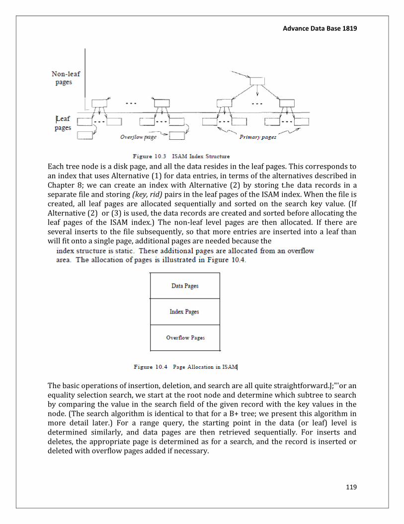
Advance Data Base 1819
119
Each tree node is a disk page, and all the data resides in the leaf pages. This corresponds to an index that uses Alternative (1) for data entries, in terms of the alternatives described in Chapter 8; we can create an index with Alternative (2) by storing t.he data records in a separate file and storing (key, rid) pairs in the leaf pages of the ISAM index. When the file is created, all leaf pages are allocated sequentially and sorted on the search key value. (If Alternative (2) or (3) is used, the data records are created and sorted before allocating the leaf pages of the ISAM index.) The non-leaf level pages are then allocated. If there are several inserts to the file subsequently, so that more entries are inserted into a leaf than will fit onto a single page, additional pages are needed because the
The basic operations of insertion, deletion, and search are all quite straightforward.J;"'or an equality selection search, we start at the root node and determine which subtree to search by comparing the value in the search field of the given record with the key values in the node. (The search algorithm is identical to that for a B+ tree; we present this algorithm in more detail later.) For a range query, the starting point in the data (or leaf) level is determined similarly, and data pages are then retrieved sequentially. For inserts and deletes, the appropriate page is determined as for a search, and the record is inserted or deleted with overflow pages added if necessary.
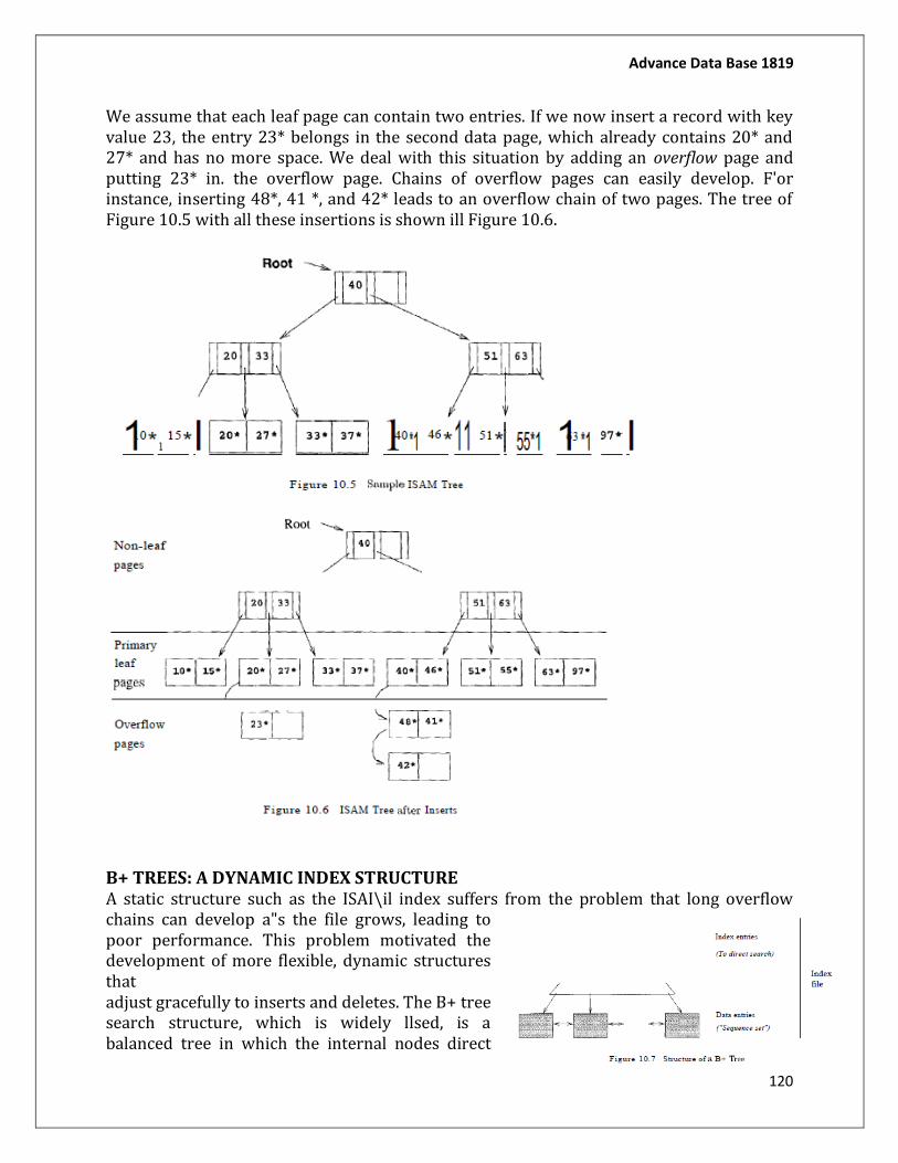
Advance Data Base 1819
120
We assume that each leaf page can contain two entries. If we now insert a record with key value 23, the entry 23* belongs in the second data page, which already contains 20* and 27* and has no more space. We deal with this situation by adding an overflow page and putting 23* in. the overflow page. Chains of overflow pages can easily develop. F'or instance, inserting 48*, 41 *, and 42* leads to an overflow chain of two pages. The tree of Figure 10.5 with all these insertions is shown ill Figure 10.6.
B+ TREES: A DYNAMIC INDEX STRUCTURE A static structure such as the ISAI\il index suffers from the problem that long overflow chains can develop a"s the file grows, leading to poor performance. This problem motivated the development of more flexible, dynamic structures that adjust gracefully to inserts and deletes. The B+ tree search structure, which is widely llsed, is a balanced tree in which the internal nodes direct
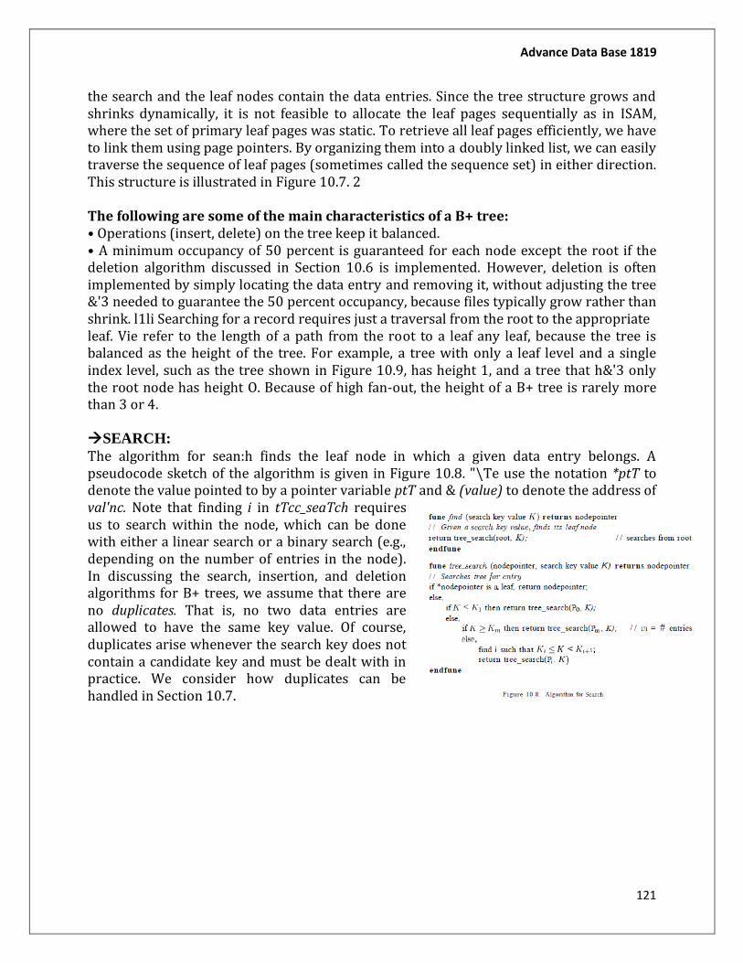
Advance Data Base 1819
121
the search and the leaf nodes contain the data entries. Since the tree structure grows and shrinks dynamically, it is not feasible to allocate the leaf pages sequentially as in ISAM, where the set of primary leaf pages was static. To retrieve all leaf pages efficiently, we have to link them using page pointers. By organizing them into a doubly linked list, we can easily traverse the sequence of leaf pages (sometimes called the sequence set) in either direction. This structure is illustrated in Figure 10.7. 2 The following are some of the main characteristics of a B+ tree: • Operations (insert, delete) on the tree keep it balanced. • A minimum occupancy of 50 percent is guaranteed for each node except the root if the deletion algorithm discussed in Section 10.6 is implemented. However, deletion is often implemented by simply locating the data entry and removing it, without adjusting the tree &'3 needed to guarantee the 50 percent occupancy, because files typically grow rather than shrink. l1li Searching for a record requires just a traversal from the root to the appropriate leaf. Vie refer to the length of a path from the root to a leaf any leaf, because the tree is balanced as the height of the tree. For example, a tree with only a leaf level and a single index level, such as the tree shown in Figure 10.9, has height 1, and a tree that h&'3 only the root node has height O. Because of high fan-out, the height of a B+ tree is rarely more than 3 or 4. SEARCH:
The algorithm for sean:h finds the leaf node in which a given data entry belongs. A pseudocode sketch of the algorithm is given in Figure 10.8. "\Te use the notation *ptT to denote the value pointed to by a pointer variable ptT and & (value) to denote the address of val'nc. Note that finding i in tTcc_seaTch requires us to search within the node, which can be done with either a linear search or a binary search (e.g., depending on the number of entries in the node). In discussing the search, insertion, and deletion algorithms for B+ trees, we assume that there are no duplicates. That is, no two data entries are allowed to have the same key value. Of course, duplicates arise whenever the search key does not contain a candidate key and must be dealt with in practice. We consider how duplicates can be handled in Section 10.7.
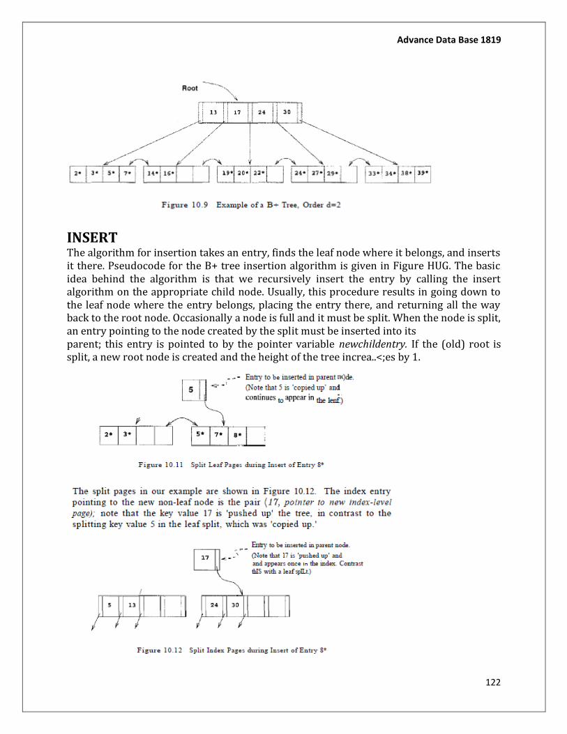
Advance Data Base 1819
122
INSERT The algorithm for insertion takes an entry, finds the leaf node where it belongs, and inserts it there. Pseudocode for the B+ tree insertion algorithm is given in Figure HUG. The basic idea behind the algorithm is that we recursively insert the entry by calling the insert algorithm on the appropriate child node. Usually, this procedure results in going down to the leaf node where the entry belongs, placing the entry there, and returning all the way back to the root node. Occasionally a node is full and it must be split. When the node is split, an entry pointing to the node created by the split must be inserted into its parent; this entry is pointed to by the pointer variable newchildentry. If the (old) root is split, a new root node is created and the height of the tree increa..<;es by 1.
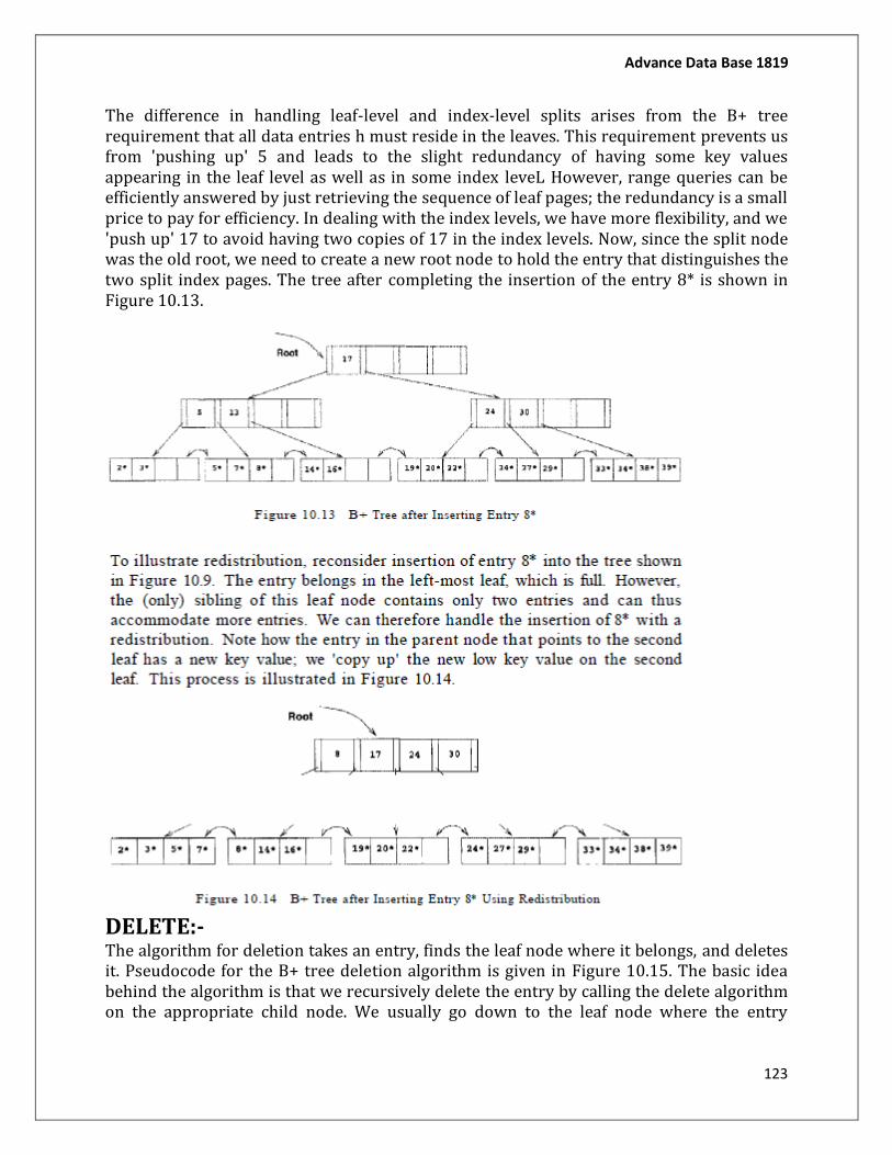
Advance Data Base 1819
123
The difference in handling leaf-level and index-level splits arises from the B+ tree requirement that all data entries h must reside in the leaves. This requirement prevents us from 'pushing up' 5 and leads to the slight redundancy of having some key values appearing in the leaf level as well as in some index leveL However, range queries can be efficiently answered by just retrieving the sequence of leaf pages; the redundancy is a small price to pay for efficiency. In dealing with the index levels, we have more flexibility, and we 'push up' 17 to avoid having two copies of 17 in the index levels. Now, since the split node was the old root, we need to create a new root node to hold the entry that distinguishes the two split index pages. The tree after completing the insertion of the entry 8* is shown in Figure 10.13.
DELETE:- The algorithm for deletion takes an entry, finds the leaf node where it belongs, and deletes it. Pseudocode for the B+ tree deletion algorithm is given in Figure 10.15. The basic idea behind the algorithm is that we recursively delete the entry by calling the delete algorithm on the appropriate child node. We usually go down to the leaf node where the entry
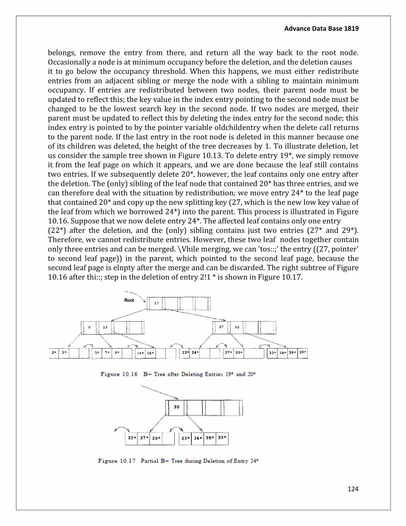
Advance Data Base 1819
124
belongs, remove the entry from there, and return all the way back to the root node. Occasionally a node is at minimum occupancy before the deletion, and the deletion causes it to go below the occupancy threshold. When this happens, we must either redistribute entries from an adjacent sibling or merge the node with a sibling to maintain minimum occupancy. If entries are redistributed between two nodes, their parent node must be updated to reflect this; the key value in the index entry pointing to the second node must be changed to be the lowest search key in the second node. If two nodes are merged, their parent must be updated to reflect this by deleting the index entry for the second node; this index entry is pointed to by the pointer variable oldchildentry when the delete call returns to the parent node. If the last entry in the root node is deleted in this manner because one of its children was deleted, the height of the tree decreases by 1. To illustrate deletion, let us consider the sample tree shown in Figure 10.13. To delete entry 19*, we simply remove it from the leaf page on which it appears, and we are done because the leaf still contains two entries. If we subsequently delete 20*, however, the leaf contains only one entry after the deletion. The (only) sibling of the leaf node that contained 20* has three entries, and we can therefore deal with the situation by redistribution; we move entry 24* to the leaf page that contained 20* and copy up the new splitting key (27, which is the new low key value of the leaf from which we borrowed 24*) into the parent. This process is illustrated in Figure 10.16. Suppose that we now delete entry 24*. The affected leaf contains only one entry (22*) after the deletion, and the (only) sibling contains just two entries (27* and 29*). Therefore, we cannot redistribute entries. However, these two leaf nodes together contain only three entries and can be merged. \Vhile merging, we can 'tos::;' the entry ((27, pointer' to second leaf page)) in the parent, which pointed to the second leaf page, because the second leaf page is elnpty after the merge and can be discarded. The right subtree of Figure 10.16 after thi::; step in the deletion of entry 2!1 * is shown in Figure 10.17.
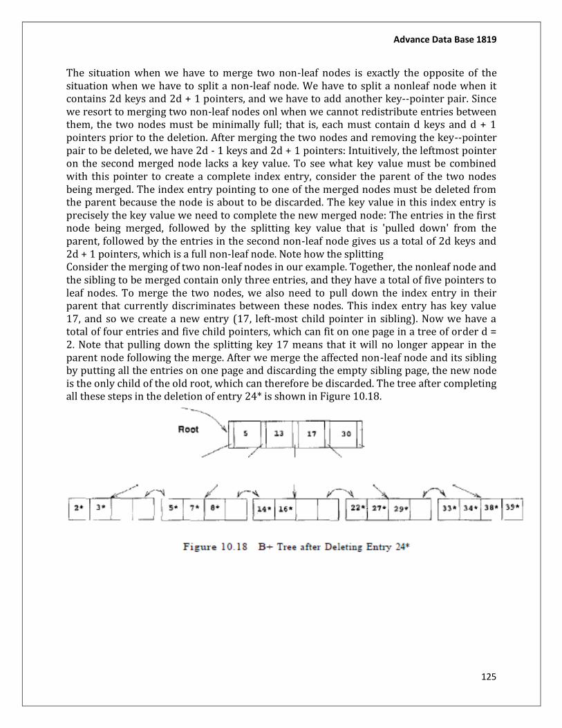
Advance Data Base 1819
125
The situation when we have to merge two non-leaf nodes is exactly the opposite of the situation when we have to split a non-leaf node. We have to split a nonleaf node when it contains 2d keys and 2d + 1 pointers, and we have to add another key--pointer pair. Since we resort to merging two non-leaf nodes onl when we cannot redistribute entries between them, the two nodes must be minimally full; that is, each must contain d keys and d + 1 pointers prior to the deletion. After merging the two nodes and removing the key--pointer pair to be deleted, we have 2d - 1 keys and 2d + 1 pointers: Intuitively, the leftmost pointer on the second merged node lacks a key value. To see what key value must be combined with this pointer to create a complete index entry, consider the parent of the two nodes being merged. The index entry pointing to one of the merged nodes must be deleted from the parent because the node is about to be discarded. The key value in this index entry is precisely the key value we need to complete the new merged node: The entries in the first node being merged, followed by the splitting key value that is 'pulled down' from the parent, followed by the entries in the second non-leaf node gives us a total of 2d keys and 2d + 1 pointers, which is a full non-leaf node. Note how the splitting Consider the merging of two non-leaf nodes in our example. Together, the nonleaf node and the sibling to be merged contain only three entries, and they have a total of five pointers to leaf nodes. To merge the two nodes, we also need to pull down the index entry in their parent that currently discriminates between these nodes. This index entry has key value 17, and so we create a new entry (17, left-most child pointer in sibling). Now we have a total of four entries and five child pointers, which can fit on one page in a tree of order d = 2. Note that pulling down the splitting key 17 means that it will no longer appear in the parent node following the merge. After we merge the affected non-leaf node and its sibling by putting all the entries on one page and discarding the empty sibling page, the new node is the only child of the old root, which can therefore be discarded. The tree after completing all these steps in the deletion of entry 24* is shown in Figure 10.18.
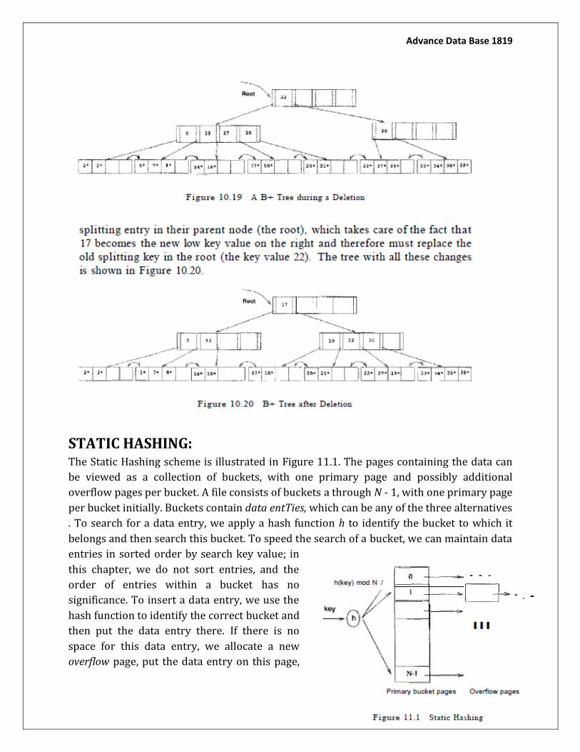
Advance Data Base 1819
126
STATIC HASHING: The Static Hashing scheme is illustrated in Figure 11.1. The pages containing the data can
be viewed as a collection of buckets, with one primary page and possibly additional
overflow pages per bucket. A file consists of buckets a through N - 1, with one primary page
per bucket initially. Buckets contain data entTies, which can be any of the three alternatives
. To search for a data entry, we apply a hash function h to identify the bucket to which it
belongs and then search this bucket. To speed the search of a bucket, we can maintain data
entries in sorted order by search key value; in
this chapter, we do not sort entries, and the
order of entries within a bucket has no
significance. To insert a data entry, we use the
hash function to identify the correct bucket and
then put the data entry there. If there is no
space for this data entry, we allocate a new
overflow page, put the data entry on this page,
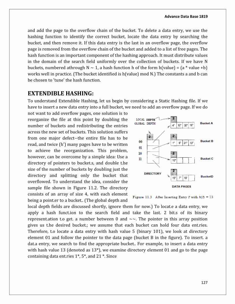
Advance Data Base 1819
127
and add the page to the overflow chain of the bucket. To delete a data entry, we use the
hashing function to identify the correct bucket, locate the data entry by searching the
bucket, and then remove it. If this data entry is the last in an overflow page, the overflow
page is removed from the overflow chain of the bucket and added to a list of free pages. The
hash function is an important component of the hashing approach. It must distribute values
in the domain of the search field uniformly over the collection of buckets. If we have N
buckets, numbered athrough N ~ 1, a hash function h of the form h(value) = (a * value +b)
works well in practice. (The bucket identified is h(value) mod N.) The constants a and b can
be chosen to 'tune' the hash function.
EXTENDIBLE HASHING: To understand Extendible Hashing, let us begin by considering a Static Hashing file. If we
have to insert a new data entry into a full bucket, we need to add an overflow page. If we do
not want to add overflow pages, one solution is to
reorganize the file at this point by doubling the
number of buckets and redistributing the entries
across the new set of buckets. This solution suffers
from one major defect--the entire file has to be
read, and twice (h') many pages have to be written
to achieve the reorganization. This problem,
however, can be overcome by a simple idea: Use a
directory of pointers to bucket.s, and double t.he
size of the number of buckets by doubling just the
directory and splitting only the bucket that
overflowed. To understand the idea, consider the
sample file shown in Figure 11.2. The directory
consists of an array of size 4, with each element
being a point.er to a bucket.. (The global depth and
local depth fields are discussed shortly, ignore them for now.) To locat.e a data entry, we
apply a hash funct.ion to the search field and take the last. 2 bit.s of its binary
represent.ation t.o get. a number between 0 and ~~. The pointer in this array position
gives us t.he desired bucket.; we assume that each bucket can hold four data ent.ries.
Therefore, t.o locate a data entry with hash value 5 (binary 101), we look at directory
element 01 and follow the pointer to the data page (bucket B in the figure). To insert. a
dat.a entry, we search to find the appropriate bucket.. For example, to insert a data entry
with hash value 13 (denoted as 13*), we examine directory element 01 and go to the page
containing data ent.ries 1*, 5*, and 21 *. Since
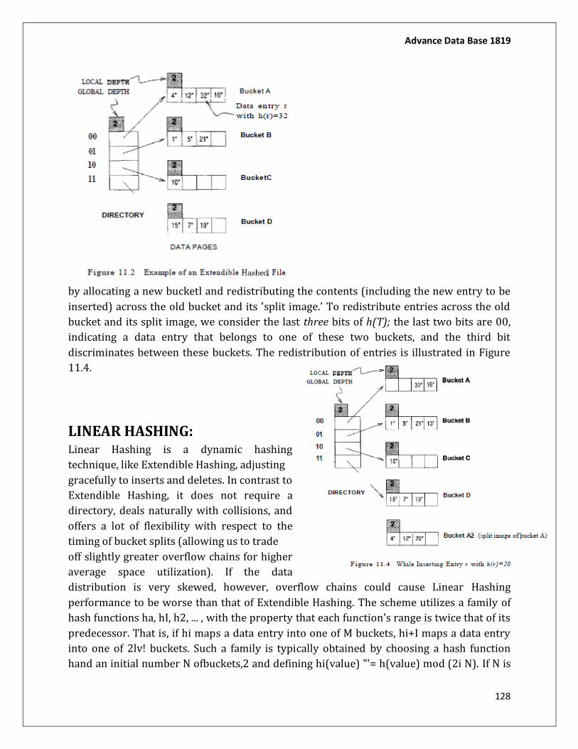
Advance Data Base 1819
128
by allocating a new bucketl and redistributing the contents (including the new entry to be
inserted) across the old bucket and its 'split image.' To redistribute entries across the old
bucket and its split image, we consider the last three bits of h(T); the last two bits are 00,
indicating a data entry that belongs to one of these two buckets, and the third bit
discriminates between these buckets. The redistribution of entries is illustrated in Figure
11.4.
LINEAR HASHING: Linear Hashing is a dynamic hashing
technique, like Extendible Hashing, adjusting
gracefully to inserts and deletes. In contrast to
Extendible Hashing, it does not require a
directory, deals naturally with collisions, and
offers a lot of flexibility with respect to the
timing of bucket splits (allowing us to trade
off slightly greater overflow chains for higher
average space utilization). If the data
distribution is very skewed, however, overflow chains could cause Linear Hashing
performance to be worse than that of Extendible Hashing. The scheme utilizes a family of
hash functions ha, hI, h2, ... , with the property that each function's range is twice that of its
predecessor. That is, if hi maps a data entry into one of M buckets, hi+I maps a data entry
into one of 2lv! buckets. Such a family is typically obtained by choosing a hash function
hand an initial number N ofbuckets,2 and defining hi(value) "'= h(value) mod (2i N). If N is

Advance Data Base 1819
129
chosen to be a power of 2, then we apply h and look at the last di bits; do is the number of
bits needed to represent N, and di = da+ i. Typically we choose h to be a function that maps
a data entry to some integer. Suppose
that we set the initial number N of buckets to be 32. In this case do is 5, and ha is therefore
h mod 32, that is, a number in the range 0 to 31. The value of dl is do + 1 = 6, and hI is h
mod (2 * 32), that is, a number in the range 0 to 63. Then h2 yields a number in the range 0
to 127, and so OIl. The idea is best understood in terms of rounds of splitting. During round
number Level, only hash functions hLeud and hLevel+1 are in use. The buckets in the file at
the beginning of the round are split, one by one from the first to the last bucket, thereby
doubling the number of buckets. At any given point within a round, therefore, we have
buckets that have been split, buckets that are yet to be split, and buckets created by splits
in this round, as illustrated in Figure 11.7. Consider how we search for a data entry with a
given search key value. \Ve apply
ha..:sh function h Level , and if this
leads us to one of the unsplit buckets,
we simply look there. If it leads us to
one of the split buckets, the entry may
be there or it may have been moved to
the new bucket created earlier in this
round by splitting this bucket; to
determine which of the two buckets
contains the entry, we apply hLevel+I'
2Note that 0 to IV - 1 is not the range
of fl.!
EXTENDIBLE VS. LINEAR HASHING:
To understand the relationship between Linear Hashing and Extendible Hashing, imagine that we also have a directory in Linear Hashing with elements 0 to N - 1. The first split is at bucket 0, and so we add directory element N. In principle, we may imagine that the entire directory has been doubled at this point; however, because element 1 is the same as element N + 1, elernent 2 is the same a.'3 element N + 2, and so on, we can avoid the actual copying for the rest of the directory. The second split occurs at bucket 1; now directory element N + 1 becomes significant and is added. At the end of the round, all the original N buckets are split, and the directory is doubled in size (because all elements point to distinct buckets). \Ve observe that the choice of hashing functions is actually very similar to what goes on in Extendible Hashing---in effect, moving from hi to hi+1 in Linear Hashing corresponds to doubling the directory in Extendible Hashing. Both operations double the effective range into which key
Advance Data Base 1819
130
values are hashed; but whereas the directory is doubled in a single step of Extendible Hashing, moving from hi to hi+l, along with a corresponding doubling in the number of buckets, occurs gradually over the course of a round in Linear Ha.'3hing. The new idea behind Linear Ha.'3hing is that a directory can be avoided by a clever choice of the bucket to split. On the other hand, by always splitting the appropriate bucket, Extendible Hashing may lead to a reduced number of splits and higher bucket occupancy. The directory analogy is useful for understanding the ideas behind Extendible and Linear Hashing. However, the directory structure can be avoided for Linear Hashing (but not for Extendible Hashing) by allocating primary bucket pages consecutively, which would allow us to locate the page for bucket i by a simple offset calculation. For uniform distributions, this implementation of Linear Hashing has a lower average cost for equality selections (because the directory level is eliminated). For skewed distributions, this implementation could result in any empty or nearly empty buckets, each of which is allocated at least one page, leading to poor performance relative to Extendible Hashing, which is likely to have higher bucket occupancy. A different implementation of Linear Hashing, in which a directory is actually maintained, offers the flexibility of not allocating one page per bucket; null directory elements can be used as in Extendible Hashing. However, this implementation introduces the overhead of a directory level and could prove costly for large, uniformly distributed files. (Also, although this implementation alleviates the potential problem of low bucket occupancy by not allocating pages for empty buckets, it is not a complete solution because we can still have many pages with very few entries.)

Advance Data Base 1819
131
UNIT-5
DISTRIBUTED DATABASES
A distributed database is a database in which storage devices are not all attached to a
common processing unit such as the CPU,[1] controlled by a distributed database
management system (together sometimes called a distributed database system). It may be
stored in multiple computers, located in the same physical location; or may be dispersed
over a network of interconnected computers. Unlike parallel systems, in which the
processors are tightly coupled and constitute a single database system, a distributed
database system consists of loosely-coupled sites that share no physical components.
System administrators can distribute collections of data (e.g. in a database) across multiple
physical locations. A distributed database can reside on network servers on theInternet, on
corporate intranets or extranets, or on other company networks. Because they store data
across multiple computers, distributed databases can improve performance at end-
user worksites by allowing transactions to be processed on many machines, instead of
being limited to one.[2]
Two processes ensure that the distributed databases remain up-to-date and
current: replication and duplication.
1. Replication involves using specialized software that looks for changes in the
distributive database. Once the changes have been identified, the replication
process makes all the databases look the same. The replication process can be
complex and time-consuming depending on the size and number of the distributed
databases. This process can also require a lot of time and computer resources.
2. Duplication, on the other hand, has less complexity. It basically identifies one
database as a master and then duplicates that database. The duplication process is
normally done at a set time after hours. This is to ensure that each distributed
location has the same data. In the duplication process, users may change only the
master database. This ensures that local data will not be overwritten.
Both replication and duplication can keep the data current in all distributive locations.
A database user accesses the distributed database through:
Local applications
applications which do not require data from other sites.
Global applications
applications which do require data from other sites.
A homogeneous distributed database has identical software and hardware running all
databases instances, and may appear through a single interface as if it were a single
Advance Data Base 1819
132
database. A heterogeneous distributed database may have different hardware, operating
systems, database management systems, and even data models for different databases.
Homogeneous DDBMS
In a homogeneous distributed database all sites have identical software and are aware of
each other and agree to cooperate in processing user requests. Each site surrenders part of
its autonomy in terms of right to change schema or software. A homogeneous DDBMS
appears to the user as a single system. The homogeneous system is much easier to design
and manage. The following conditions must be satisfied for homogeneous database:
The operating system used, at each location must be same or compatible.
The data structures used at each location must be same or compatible.
The database application (or DBMS) used at each location must be same or compatible.
Heterogeneous DDBMS
In a heterogeneous distributed database, different sites may use different schema and
software. Difference in schema is a major problem for query processing and transaction
processing. Sites may not be aware of each other and may provide only limited facilities for
cooperation in transaction processing. In heterogeneous systems, different nodes may have
different hardware & software and data structures at various nodes or locations are also
incompatible. Different computers and operating systems, database applications or data
models may be used at each of the locations. For example, one location may have the latest
relational database management technology, while another location may store data using
conventional files or old version of database management system. Similarly, one location
may have the Windows NT operating system, while another may have UNIX.
Heterogeneous systems are usually used when individual sites use their own hardware and
software. On heterogeneous system, translations are required to allow communication
between different sites (or DBMS). In this system, the users must be able to make requests
in a database language at their local sites. Usually the SQL database language is used for
this purpose. If the hardware is different, then the translation is straightforward, in which
computer codes and word-length is changed. The heterogeneous system is often not
technically or economically feasible. In this system, a user at one location may be able to
read but not update the data at another location.
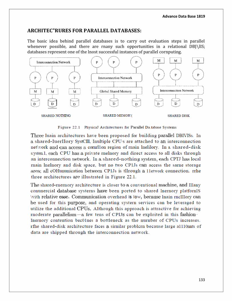
Advance Data Base 1819
133
ARCHITEC"RURES FOR PARALLEL DATABASES:
The basic idea behind parallel databases is to carry out evaluation steps in parallel whenever possible, and there are rnany such opportunities in a relational DBJ\lIS; databases represent one of the lnost successful instances of parallel cornputing.

Advance Data Base 1819
134
Distributed Database Architecture
A distributed database system allows applications to access data from local and remote databases. In a homogenous distributed database system, each database is an Oracle Database. In a heterogeneous distributed database system, at least one of the databases is not an Oracle Database. Distributed databases use a client/server architecture to process information requests.
This section contains the following topics:
Homogenous Distributed Database Systems Heterogeneous Distributed Database Systems Client/Server Database Architecture
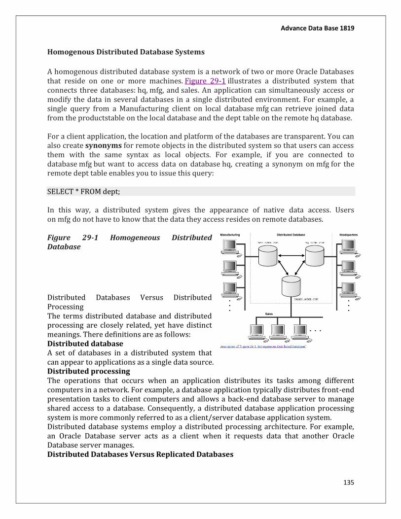
Advance Data Base 1819
135
Homogenous Distributed Database Systems
A homogenous distributed database system is a network of two or more Oracle Databases that reside on one or more machines. Figure 29-1 illustrates a distributed system that connects three databases: hq, mfg, and sales. An application can simultaneously access or modify the data in several databases in a single distributed environment. For example, a single query from a Manufacturing client on local database mfg can retrieve joined data from the productstable on the local database and the dept table on the remote hq database.
For a client application, the location and platform of the databases are transparent. You can also create synonyms for remote objects in the distributed system so that users can access them with the same syntax as local objects. For example, if you are connected to database mfg but want to access data on database hq, creating a synonym on mfg for the remote dept table enables you to issue this query:
SELECT * FROM dept;
In this way, a distributed system gives the appearance of native data access. Users on mfg do not have to know that the data they access resides on remote databases.
Figure 29-1 Homogeneous Distributed Database
Distributed Databases Versus Distributed Processing The terms distributed database and distributed processing are closely related, yet have distinct meanings. There definitions are as follows: Distributed database A set of databases in a distributed system that can appear to applications as a single data source. Distributed processing The operations that occurs when an application distributes its tasks among different computers in a network. For example, a database application typically distributes front-end presentation tasks to client computers and allows a back-end database server to manage shared access to a database. Consequently, a distributed database application processing system is more commonly referred to as a client/server database application system. Distributed database systems employ a distributed processing architecture. For example, an Oracle Database server acts as a client when it requests data that another Oracle Database server manages. Distributed Databases Versus Replicated Databases
Advance Data Base 1819
136
The terms distributed database system and database replication are related, yet distinct. In a pure (that is, not replicated) distributed database, the system manages a single copy of all data and supporting database objects. Typically, distributed database applications use distributed transactions to access both local and remote data and modify the global database in real-time.
Heterogeneous Distributed Database Systems In a heterogeneous distributed database system, at least one of the databases is a non-Oracle Database system. To the application, the heterogeneous distributed database system appears as a single, local, Oracle Database. The local Oracle Database server hides the distribution and heterogeneity of the data. The Oracle Database server accesses the non-Oracle Database system using Oracle Heterogeneous Services in conjunction with an agent. If you access the non-Oracle Database data store using an Oracle Transparent Gateway, then the agent is a system-specific application. For example, if you include a Sybase database in an Oracle Database distributed system, then you need to obtain a Sybase-specific transparent gateway so that the Oracle Database in the system can communicate with it. Alternatively, you can use generic connectivity to access non-Oracle Database data stores so long as the non-Oracle Database system supports the ODBC or OLE DB protocols.
Heterogeneous Services
Heterogeneous Services (HS) is an integrated component within the Oracle Database server and the enabling technology for the current suite of Oracle Transparent Gateway products. HS provides the common architecture and administration mechanisms for Oracle Database gateway products and other heterogeneous access facilities. Also, it provides upwardly compatible functionality for users of most of the earlier Oracle Transparent Gateway releases.
Transparent Gateway Agents
For each non-Oracle Database system that you access, Heterogeneous Services can use a transparent gateway agent to interface with the specified non-Oracle Database system. The agent is specific to the non-Oracle Database system, so each type of system requires a different agent.
The transparent gateway agent facilitates communication between Oracle Database and non-Oracle Database systems and uses the Heterogeneous Services component in the Oracle Database server. The agent executes SQL and transactional requests at the non-Oracle Database system on behalf of the Oracle Database server.
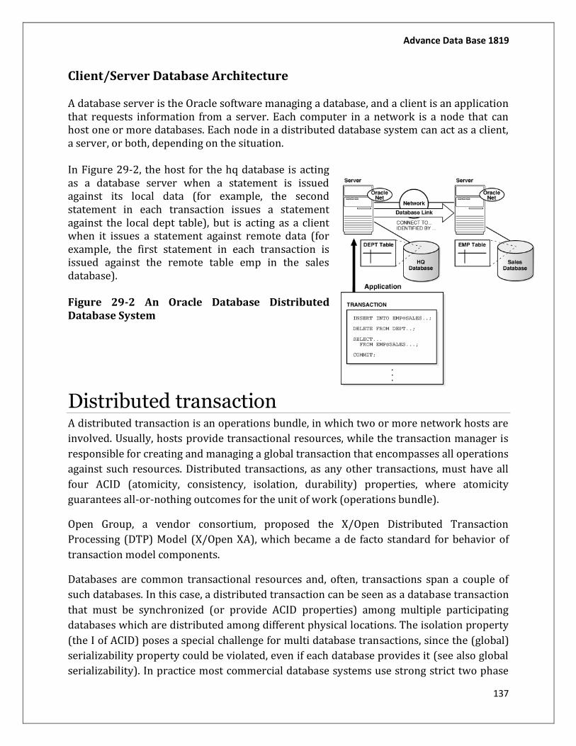
Advance Data Base 1819
137
Client/Server Database Architecture A database server is the Oracle software managing a database, and a client is an application that requests information from a server. Each computer in a network is a node that can host one or more databases. Each node in a distributed database system can act as a client, a server, or both, depending on the situation. In Figure 29-2, the host for the hq database is acting as a database server when a statement is issued against its local data (for example, the second statement in each transaction issues a statement against the local dept table), but is acting as a client when it issues a statement against remote data (for example, the first statement in each transaction is issued against the remote table emp in the sales database). Figure 29-2 An Oracle Database Distributed Database System
Distributed transaction A distributed transaction is an operations bundle, in which two or more network hosts are
involved. Usually, hosts provide transactional resources, while the transaction manager is
responsible for creating and managing a global transaction that encompasses all operations
against such resources. Distributed transactions, as any other transactions, must have all
four ACID (atomicity, consistency, isolation, durability) properties, where atomicity
guarantees all-or-nothing outcomes for the unit of work (operations bundle).
Open Group, a vendor consortium, proposed the X/Open Distributed Transaction
Processing (DTP) Model (X/Open XA), which became a de facto standard for behavior of
transaction model components.
Databases are common transactional resources and, often, transactions span a couple of
such databases. In this case, a distributed transaction can be seen as a database transaction
that must be synchronized (or provide ACID properties) among multiple participating
databases which are distributed among different physical locations. The isolation property
(the I of ACID) poses a special challenge for multi database transactions, since the (global)
serializability property could be violated, even if each database provides it (see also global
serializability). In practice most commercial database systems use strong strict two phase
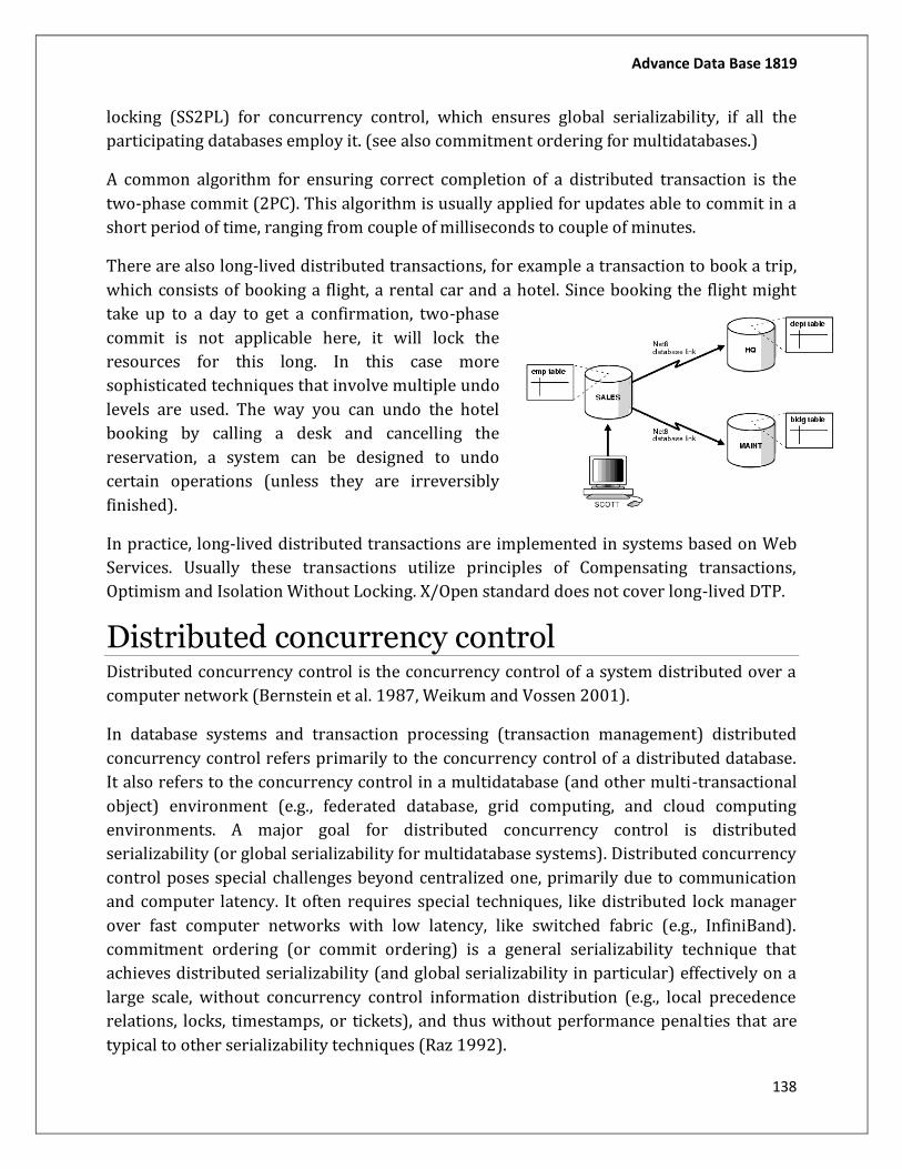
Advance Data Base 1819
138
locking (SS2PL) for concurrency control, which ensures global serializability, if all the
participating databases employ it. (see also commitment ordering for multidatabases.)
A common algorithm for ensuring correct completion of a distributed transaction is the
two-phase commit (2PC). This algorithm is usually applied for updates able to commit in a
short period of time, ranging from couple of milliseconds to couple of minutes.
There are also long-lived distributed transactions, for example a transaction to book a trip,
which consists of booking a flight, a rental car and a hotel. Since booking the flight might
take up to a day to get a confirmation, two-phase
commit is not applicable here, it will lock the
resources for this long. In this case more
sophisticated techniques that involve multiple undo
levels are used. The way you can undo the hotel
booking by calling a desk and cancelling the
reservation, a system can be designed to undo
certain operations (unless they are irreversibly
finished).
In practice, long-lived distributed transactions are implemented in systems based on Web
Services. Usually these transactions utilize principles of Compensating transactions,
Optimism and Isolation Without Locking. X/Open standard does not cover long-lived DTP.
Distributed concurrency control Distributed concurrency control is the concurrency control of a system distributed over a
computer network (Bernstein et al. 1987, Weikum and Vossen 2001).
In database systems and transaction processing (transaction management) distributed
concurrency control refers primarily to the concurrency control of a distributed database.
It also refers to the concurrency control in a multidatabase (and other multi-transactional
object) environment (e.g., federated database, grid computing, and cloud computing
environments. A major goal for distributed concurrency control is distributed
serializability (or global serializability for multidatabase systems). Distributed concurrency
control poses special challenges beyond centralized one, primarily due to communication
and computer latency. It often requires special techniques, like distributed lock manager
over fast computer networks with low latency, like switched fabric (e.g., InfiniBand).
commitment ordering (or commit ordering) is a general serializability technique that
achieves distributed serializability (and global serializability in particular) effectively on a
large scale, without concurrency control information distribution (e.g., local precedence
relations, locks, timestamps, or tickets), and thus without performance penalties that are
typical to other serializability techniques (Raz 1992).
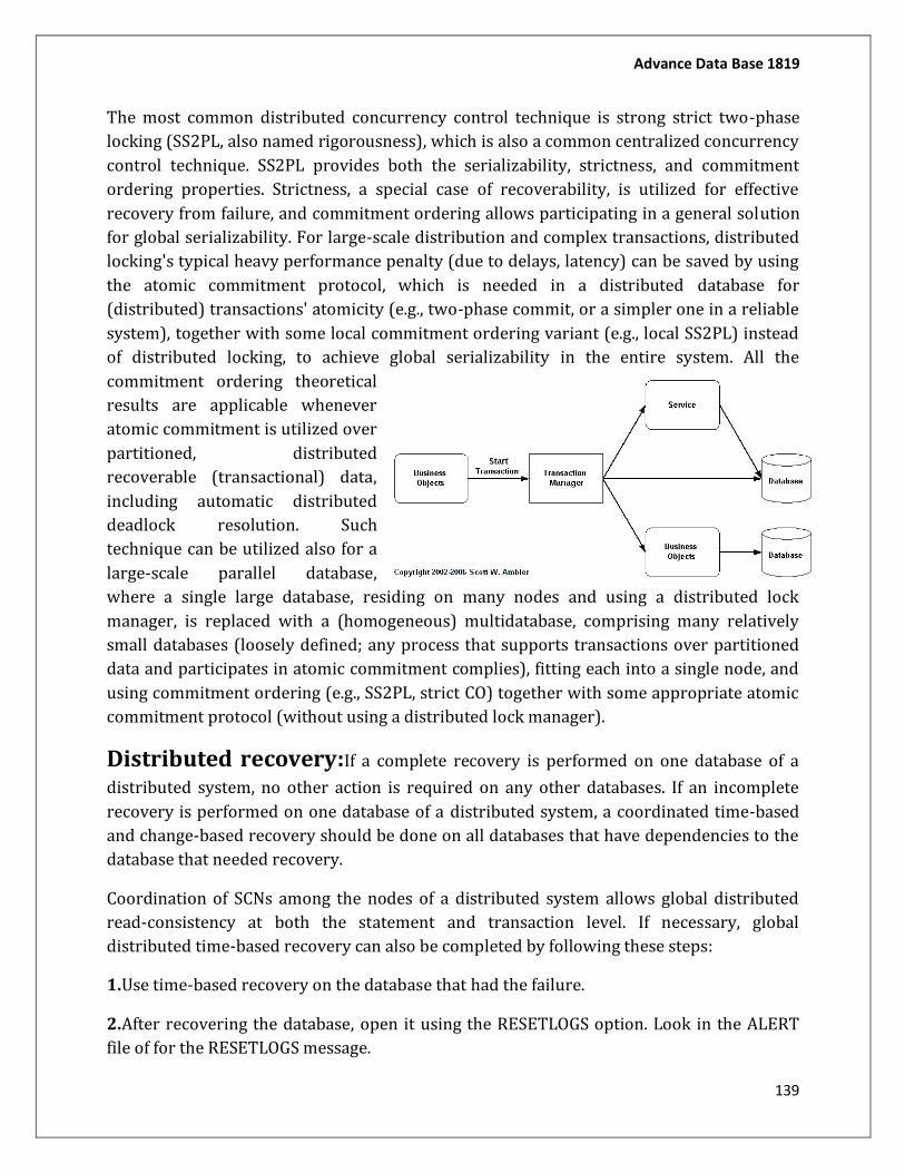
Advance Data Base 1819
139
The most common distributed concurrency control technique is strong strict two-phase
locking (SS2PL, also named rigorousness), which is also a common centralized concurrency
control technique. SS2PL provides both the serializability, strictness, and commitment
ordering properties. Strictness, a special case of recoverability, is utilized for effective
recovery from failure, and commitment ordering allows participating in a general solution
for global serializability. For large-scale distribution and complex transactions, distributed
locking's typical heavy performance penalty (due to delays, latency) can be saved by using
the atomic commitment protocol, which is needed in a distributed database for
(distributed) transactions' atomicity (e.g., two-phase commit, or a simpler one in a reliable
system), together with some local commitment ordering variant (e.g., local SS2PL) instead
of distributed locking, to achieve global serializability in the entire system. All the
commitment ordering theoretical
results are applicable whenever
atomic commitment is utilized over
partitioned, distributed
recoverable (transactional) data,
including automatic distributed
deadlock resolution. Such
technique can be utilized also for a
large-scale parallel database,
where a single large database, residing on many nodes and using a distributed lock
manager, is replaced with a (homogeneous) multidatabase, comprising many relatively
small databases (loosely defined; any process that supports transactions over partitioned
data and participates in atomic commitment complies), fitting each into a single node, and
using commitment ordering (e.g., SS2PL, strict CO) together with some appropriate atomic
commitment protocol (without using a distributed lock manager).
Distributed recovery:If a complete recovery is performed on one database of a
distributed system, no other action is required on any other databases. If an incomplete
recovery is performed on one database of a distributed system, a coordinated time-based
and change-based recovery should be done on all databases that have dependencies to the
database that needed recovery.
Coordination of SCNs among the nodes of a distributed system allows global distributed
read-consistency at both the statement and transaction level. If necessary, global
distributed time-based recovery can also be completed by following these steps:
1.Use time-based recovery on the database that had the failure.
2.After recovering the database, open it using the RESETLOGS option. Look in the ALERT
file of for the RESETLOGS message.
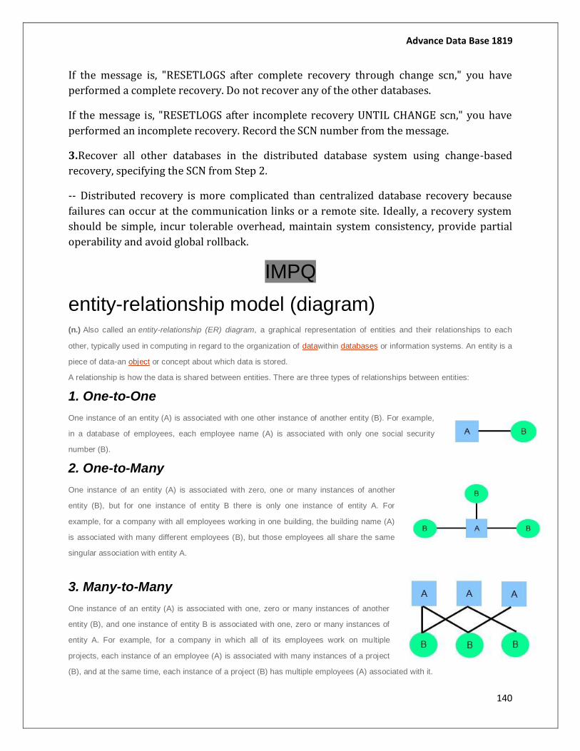
Advance Data Base 1819
140
If the message is, "RESETLOGS after complete recovery through change scn," you have
performed a complete recovery. Do not recover any of the other databases.
If the message is, "RESETLOGS after incomplete recovery UNTIL CHANGE scn," you have
performed an incomplete recovery. Record the SCN number from the message.
3.Recover all other databases in the distributed database system using change-based
recovery, specifying the SCN from Step 2.
-- Distributed recovery is more complicated than centralized database recovery because
failures can occur at the communication links or a remote site. Ideally, a recovery system
should be simple, incur tolerable overhead, maintain system consistency, provide partial
operability and avoid global rollback.
IMPQ
entity-relationship model (diagram) (n.) Also called an entity-relationship (ER) diagram, a graphical representation of entities and their relationships to each
other, typically used in computing in regard to the organization of datawithin databases or information systems. An entity is a
piece of data-an object or concept about which data is stored.
A relationship is how the data is shared between entities. There are three types of relationships between entities:
1. One-to-One
One instance of an entity (A) is associated with one other instance of another entity (B). For example,
in a database of employees, each employee name (A) is associated with only one social security
number (B).
2. One-to-Many
One instance of an entity (A) is associated with zero, one or many instances of another
entity (B), but for one instance of entity B there is only one instance of entity A. For
example, for a company with all employees working in one building, the building name (A)
is associated with many different employees (B), but those employees all share the same
singular association with entity A.
3. Many-to-Many
One instance of an entity (A) is associated with one, zero or many instances of another
entity (B), and one instance of entity B is associated with one, zero or many instances of
entity A. For example, for a company in which all of its employees work on multiple
projects, each instance of an employee (A) is associated with many instances of a project
(B), and at the same time, each instance of a project (B) has multiple employees (A) associated with it.
Advance Data Base 1819
141
Overview of Logical Design
This chapter tells how to design a data warehousing environment, and includes the following topics:
Logical vs. Physical Create a Logical Design Data Warehousing Schemas
Logical vs. Physical
If you are reading this guide, it is likely that your organization has already decided to build a data warehouse. Moreover, it is likely that the business requirements are already defined, the scope of your application has been agreed upon, and you have a conceptual design. So now you need to translate your requirements into a system deliverable. In this step, you create the logical and physical design for the data warehouse and, in the process, define the specific data content, relationships within and between groups of data, the system environment supporting your data warehouse, the data transformations required, and the frequency with which data is refreshed.
The logical design is more conceptual and abstract than the physical design. In the logical design, you look at the logical relationships among the objects. In the physical design, you look at the most effective way of storing and retrieving the objects.
Your design should be oriented toward the needs of the end users. End users typically want to perform analysis and look at aggregated data, rather than at individual transactions. Your design is driven primarily by end-user utility, but the end users may not know what they need until they see it. A well-planned design allows for growth and changes as the needs of users change and evolve.
By beginning with the logical design, you focus on the information requirements without getting bogged down immediately with implementation detail.
Create a Logical Design
A logical design is a conceptual, abstract design. You do not deal with the physical implementation details yet; you deal only with defining the types of information that you need.
The process of logical design involves arranging data into a series of logical relationships called entities and attributes. An entity represents a chunk of information. In relational
Advance Data Base 1819
142
databases, an entity often maps to a table. Anattribute is a component of an entity and helps define the uniqueness of the entity. In relational databases, an attribute maps to a column.
You can create the logical design using a pen and paper, or you can use a design tool such as Oracle Warehouse Builder or Oracle Designer.
While entity-relationship diagramming has traditionally been associated with highly normalized models such as online transaction processing (OLTP) applications, the technique is still useful in dimensional modeling. You just approach it differently. In dimensional modeling, instead of seeking to discover atomic units of information and all of the relationships between them, you try to identify which information belongs to a central fact table(s) and which information belongs to its associated dimension tables.
One output of the logical design is a set of entities and attributes corresponding to fact tables and dimension tables. Another output of mapping is operational data from your source into subject-oriented information in your target data warehouse schema. You identify business subjects or fields of data, define relationships between business subjects, and name the attributes for each subject.
The elements that help you to determine the data warehouse schema are the model of your source data and your user requirements. Sometimes, you can get the source model from your company's enterprise data model and reverse-engineer the logical data model for the data warehouse from this. The physical implementation of the logical data warehouse model may require some changes due to your system parameters--size of machine, number of users, storage capacity, type of network, and software.
Data Warehousing Schemas
A schema is a collection of database objects, including tables, views, indexes, and synonyms. There are a variety of ways of arranging schema objects in the schema models designed for data warehousing. Most data warehouses use a dimensional model.
Star Schemas
The star schema is the simplest data warehouse schema. It is called a star schema because the diagram of a star schema resembles a star, with points radiating from a center. The center of the star consists of one or more fact tables and the points of the star are the dimension tables shown in Figure 2-1:
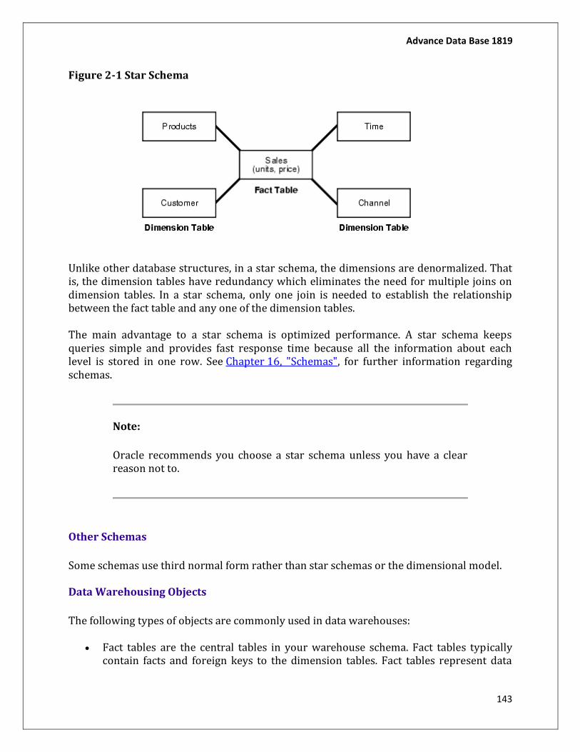
Advance Data Base 1819
143
Figure 2-1 Star Schema
Unlike other database structures, in a star schema, the dimensions are denormalized. That is, the dimension tables have redundancy which eliminates the need for multiple joins on dimension tables. In a star schema, only one join is needed to establish the relationship between the fact table and any one of the dimension tables.
The main advantage to a star schema is optimized performance. A star schema keeps queries simple and provides fast response time because all the information about each level is stored in one row. See Chapter 16, "Schemas", for further information regarding schemas.
Note:
Oracle recommends you choose a star schema unless you have a clear reason not to.
Other Schemas
Some schemas use third normal form rather than star schemas or the dimensional model.
Data Warehousing Objects
The following types of objects are commonly used in data warehouses:
Fact tables are the central tables in your warehouse schema. Fact tables typically contain facts and foreign keys to the dimension tables. Fact tables represent data
Advance Data Base 1819
144
usually numeric and additive that can be analyzed and examined. Examples include Sales, Cost, and Profit.
Dimension tables, also known as lookup or reference tables, contain the relatively static data in the warehouse. Examples are stores or products.
Fact Tables
A fact table is a table in a star schema that contains facts. A fact table typically has two types of columns: those that contain facts, and those that are foreign keys to dimension tables. A fact table might contain either detail-level facts or facts that have been aggregated. Fact tables that contain aggregated facts are often called summary tables. A fact table usually contains facts with the same level of aggregation.
Values for facts or measures are usually not known in advance; they are observed and stored.
Fact tables are the basis for the data queried by OLAP tools.
Creating a New Fact Table
You must define a fact table for each star schema. A fact table typically has two types of columns: those that contain facts, and those that are foreign keys to dimension tables. From a modeling standpoint, the primary key of the fact table is usually a composite key that is made up of all of its foreign keys; in the physical data warehouse, the data warehouse administrator may or may not choose to create this primary key explicitly.
Facts support mathematical calculations used to report on and analyze the business. Some numeric data are dimensions in disguise, even if they seem to be facts. If you are not interested in a summarization of a particular item, the item may actually be a dimension. Database size and overall performance improve if you categorize borderline fields as dimensions.
Dimensions
A dimension is a structure, often composed of one or more hierarchies, that categorizes data. Several distinct dimensions, combined with measures, enable you to answer business questions. Commonly used dimensions are Customer, Product, and Time. Figure 2-2 shows some a typical dimension hierarchy.

Advance Data Base 1819
145
Figure 2-2 Typical Levels in a Dimension Hierarchy
Dimension data is typically collected at the lowest level of detail and then aggregated into higher level totals, which is more useful for analysis. For example, in the Total_Customer dimension, there are four levels: Total_Customer, Regions, Territories, and Customers. Data collected at the Customers level is aggregated to the Territories level. For the Regions dimension, data collected for several regions such as Western Europe or Eastern Europe might be aggregated as a fact in the fact table into totals for a larger area such as Europe.