ADirectImagingMethodforInverseElectromagnetic … Scattering Problem in Rectangular Waveguide...

Commun. Comput. Phys.doi: 10.4208/cicp.OA-2017-0048

Vol. 23, No. 5, pp. 1415-1433May 2018

A Direct Imaging Method for Inverse Electromagnetic

Scattering Problem in Rectangular Waveguide

Junqing Chen1,∗ and Guanghui Huang2

1 Department of Mathematical Sciences, Tsinghua University, Beijing 10084,P.R. China.2 The Rice Inversion Project, Department of Computational andApplied Mathematics, Rice University, Houston, TX 77005-1892, USA.

Received 10 March 2017; Accepted (in revised version) 8 August 2017

Abstract. We propose a direct imaging method based on reverse time migration (RTM)algorithm for imaging extended targets using electromagnetic waves at a fixed fre-quency in the rectangular waveguide. The imaging functional is defined as the imagi-nary part of the cross-correlation of the Green function for Helmholtz equation and theback-propagated electromagnetic field. The resolution of our RTM method for pene-trable extended targets is studied by virtue of Helmholtz-Kirchhoff identity in the rect-angular domain, which implies that the imaging functional always peaks in the target.Numerical examples are provided to demonstrate the powerful imaging quality andconfirm our theoretical results.

AMS subject classifications: 65N21, 78A46

Key words: Electromagnetic waveguide, inverse scattering problem, reverse time migration, ex-tended obstacle.

1 Introduction

Imaging the dielectric obstacles or biological objects in the rectangular waveguides is aquite important subject in the microwave medical imaging and specimen nondestructivetesting. In this paper we propose a reverse time migration (RTM) method to find thesupport of an unknown obstacle embedded in a rectangular electromagnetic waveguidefrom the measurement of the wave field which is far away from the obstacle (see Fig. 1).Let R3

ab=(x1,x2,x3)∈R3 :x1∈(0,a),x2∈(0,b),x3∈R be the rectangular waveguide withthe rectangular cross section. Denote by Γ0a=(x1,x2,x3)∈R3:x1=0 or x1=a,x2∈(0,b),x3∈R and Γ0b=(x1,x2,x3)∈R3 :x2=0 or x2=b,x1∈(0,a),x3∈R the boundaries of R3

ab. Let

∗Corresponding author. Email addresses: [email protected] (J. Chen), [email protected](G. Huang)

http://www.global-sci.com/ 1415 c©2018 Global-Science Press

1416 J. Chen and G. Huang / Commun. Comput. Phys., 23 (2018), pp. 1415-1433

Figure 1: The geometric setting of the electromagnetic scattering problem in rectangular waveguide.

the obstacle occupy a bounded Lipschitz domain D included in Bρ=(0,a)×(0,b)×(−ρ,ρ),ρ>0, with ν the unit outer normal to its boundary ΓD. We assume the incident wave is apoint source excited at xs. The measured wave field satisfies the following equations:

curlcurlE−k2n(x)E=δxs(x)p in R3ab, (1.1)

ν×E=0 on Γ0a∪Γ0b, (1.2)

and a radiation condition at infinity which will be stated in the following. Where k> 0is the wave number, n∈ L∞(R3

ab) is a positive scalar function and n(x)−1 is compactlysupported in D, δxs is the Dirac source located at xs ∈R3

ab, p ∈R3, |p|= 1, is the polar-ization direction of the source. We remark that the results in this paper also apply tonon-penetrable obstacles with other boundary conditions on the scatterer.

Now we introduce the radiation condition for completing the systems of (1.1)-(1.2).

Let (λ(1)j ,Φ

(1)j ) and (λ

(2)j ,Φ

(2)j ) be the complete systems of eigenvalues and orthonormal

eigenfunctions in the sense of L2 of the two-dimensional Laplace operator −∆ with theDirichlet and Neumann boundary conditions respectively. For large enough R> 0 and|x3|>R, we impose the similar condition introduced in [25],

E(x)=∑j

E1±j e

iγ(1)j |x3|(λ(1)

j Φ(1)j e3+isign(x3)γ

(1)j ∇2Φ

(1)j )

+ik∑j

E2±j e

iγ(2)j |x3|∇2Φ

(2)j ×e3, (1.3)

where ∇2 = e1∂

∂x1+e2

∂∂x2

, γ(p)j =

√

k2−λ(p)j , p= 1,2, and we choose the branch cut of

√z

such that Im(√

z)≥0 throughout the paper.In the last two decades, direct sampling methods have drawn considerable attentions

in the field concerning inverse scattering problems. Among these direct methods, thelinear sampling method [14], factorization method [16, 20] and MUSIC method [2, 7] arequite popular. There are also some other direct sampling methods successfully appliedto inverse scattering problems in the free space such as [18,19] and the references therein.Due to the multiple scattering by boundaries of waveguide, imaging a scatterer in thewaveguide is much more challenging than in the free space [11]. We refer to [6,28,30] for

J. Chen and G. Huang / Commun. Comput. Phys., 23 (2018), pp. 1415-1433 1417

linear sampling method to imaging the extended obstacles, and [29] for selected imagingmethod to locate the reflectors. See also [17] for eigensystem decomposition methodin 2D and [3] for factorization method in 3D to reconstruct the inhomogeneities in theacoustic waveguide setting.

The RTM method, which consists of back-propagating the complex conjugated datainto the background medium and computing the cross-correlation between the incidentwave field and the back-propagation field to output the final imaging profile, is nowa-days widely used in exploration geophysics [4, 5, 13]. In [9, 10], the RTM method forreconstructing extended targets using acoustic and electromagnetic waves at a fixed fre-quency in the free space is proposed and studied. The resolution analysis in [9, 10] isachieved without using the small inclusion or geometrical optics assumption previouslymade in the literatures. More interestingly, the authors have generalized the reverse timemigration method for reconstructing the extended obstacles in the planar acoustic waveg-uide, in which the data is only available within the limited aperture [11], and they alsoprove that the same imaging resolution can be guaranteed assuming that appropriateacquisition aperture is chosen in terms of the wavenumber and thickness of waveguide.

In this paper, we extend the RTM method in [9–11] to find extended targets in theelectromagnetic rectangular waveguide. Our new RTM algorithm is motivated by theHelmholtz-Kirchhoff identity for the waveguide scattering problems. We show our newimaging function also enjoys the nice feature that it is always positive and thus may havebetter stability properties.

The rest of this paper is organized as follows. In Section 2, we introduce some prelim-inary results concerning about electromagnetic direct scattering problem in rectangularwaveguide. In Section 3, we propose a direct imaging method based on reverse timemigration method. In Section 4, we present resolution analysis of our imaging method.Finally, in Section 5, we report several numerical experiments to demonstrate the power-ful imaging quality of our algorithm with full 3D electromagnetic waveguide data.

2 Direct scattering problem

We start by introducing the Green function G(x,y), which is the radiation solution satis-fying the equations:

curlcurlG(x,y)−k2G(x,y)=Iδy(x) in R

3ab,

ν×G(x,y)=0 on Γ0a∪Γ0b.

Following the description of [25], the Green function can be expressed as

G(x,y)=(

I+∇x∇x

k2

)

gD(x,y), (2.1)

where I is the 3×3 identity matrix and gD(x,y)=diag(

g1(x,y),g2(x,y),g3(x,y))

. gj(x,y)(j=1,2,3) satisfy the Helmholtz equation,

∆gj(x,y)+k2gj(x,y)=−δy(x) in R3ab. (2.2)


and the boundary conditions

∂g1

∂x1

∣

∣

∣

x1− a2=± a

2

=0, g1|x2− b2=± b

2=0,

g2|x1− a2=± a

2=0,

∂g2

∂x2

∣

∣

∣

x2− b2=± b

2

=0,

g3

∣

∣

∣

x1− a2=± a

2

=0, g3|x2− b2=± b

2=0,

together with the radiation condition which guarantees gj(x,y) (j= 1,2,3) are outgoingwaves at infinity alone ±x3 directions. Denote by the set Cj(j=1,2,3)

C1=(m,n)|m∈N,n∈N+,

C2=(m,n)|m∈N+,n∈N,

C3=(m,n)|m∈N+,n∈N

+.

It is given in [25] that

gj(x,y)= ∑(m,n)∈Cj

gmn(x3,y3)φjmn(x1,x2)φ

jmn(y1,y2), (2.3)

where the mode expansion coefficients gmn(x3,y3)=ieiµmn|x3−y3|

2µmnand basis functions φ

jmn

are given by

φ1mn(x1,x2)=

2√

ab(1+δ0m)cos

mπ

ax1sin

nπ

bx2, (m,n)∈C1,

φ2mn(x1,x2)=

2√

ab(1+δ0n)sin

mπ

ax1cos

nπ

bx2, (m,n)∈C2,

φ3mn(x1,x2)=

2√ab

sinmπ

ax1sin

nπ

bx2, (m,n)∈C3,

and µmn =√

k2−λ2mn (λmn=π

√

(

ma

)2+(

nb

)2,(m,n)∈C1∪C2).

Throughout this paper, we assume that,

k 6=λmn, ∀(m,n)∈C1∪C2. (2.4)

Now, we consider the direct electromagnetic scattering problem in rectangular waveg-uide,

curlcurlU−k2n(x)U= f (x) in R3ab, (2.5)

ν×U=0 on Γ0a∪Γ0b. (2.6)


Lemma 2.1. Assume that n(x)−1 is piecewise smooth and compactly supported in D and f ∈L2(R3

ab) has compact support. Then the problem (2.5)-(2.6) admits a unique radiation solutionU∈Hloc(curl;R3

ab). Moreover, there exists a constant C such that ‖U‖H(curl;D)≤C‖ f‖L2(R3ab)

.

The proof of the above lemma can be found in [25] by integral equation method. ByLemma 2.1, we can introduce the solution operator S : L2(R3

ab)→ H(curl;D) by U = S fwhich maps the scattering source f into the scattering field U∈H(curl;D). In this paperwe will denote by ‖S‖ the operator norm of S which depends generally on a,b,k,n(x) andthe domain D.

To proceed, we need the following lemma.

Lemma 2.2. Let Φ(1)j ,Φ

(2)l be the eigenfunctions of 2-D Laplace operator −∆ with the Dirichlet

and Neumann condition on the boundary of rectangle domain [0,a]×[0,b] as in (1.2), we havethat

∫

Γ±R

e3×∇2Φ(2)l ·∇2Φ

(1)j ds=0, (2.7)

where Γ±R =(x1,x2,x3)∈R3 : x1∈ (0,a),x2 ∈ (0,b),x3=±R.

Proof. We only prove that the above integral is vanishing on Γ+R , the other one can be

obtained in the same way. Note that e3×∇2Φ(2)l =−∇2×(Φ

(2)l e3), then

∫

ΓR

e3×∇2Φ(2)l ·Φ(1)

j ds=−∫

ΓR

∇2×(Φ(2)l e3)·∇2Φ

(1)j ds

=−∫

ΓR

∇2×Φ(2)l ·∇2Φ

(1)j ds,

where ∇2× is the 2-D vector curl operator and ∇2 is the 2-D gradient operator.By integration by part, we have

∫

ΓR

∇2×Φ(2)l ·∇2Φ

(1)j ds=

∫

∂ΓR

n·∇2×Φ(2)l Φ

(1)j dγ.

By the boundary condition satisfied by Φ(1)j , the above equation is vanishing, which com-

pletes the proof.

Lemma 2.3. Assume that U is the radiation solution of the scattering problem (2.5)-(2.6) withf ∈L2(R3

ab) compactly supported in D. Then we have

Im〈U, f 〉D = k2

( J1

∑j=1

λ(1)j γ

(1)j (|U1+

j |2+|U1−j |2)+

J2

∑j=1

γ(2)j λ

(2)j (|U2+

j |2+|U2−j |2)

)

>0,

where 〈U, f 〉D=∫

D U · f dx, Jp is the maximum number such that λ(p)j <k holds, and U

p±j are the

propagation modes, p=1,2.


Proof. By (2.5) and integration by parts, we have∫

Df ·Udx=

∫

BR

f ·Udx=∫

BR

(

curlcurlU−k2n(x)U)

·Udx

=∫

∂BR

ν×curlU·Uds(x)+∫

BR

|curlU|2−k2n(x)|U|2dx,

where BR=[0,a]×[0,b]×[−R,R].By the boundary condition satisfied by U,

∫

(Γ0a∪Γ0b)∩∂BRν×U·curlUds(x)= 0. Taking

the imaginary part of the above formula, we have

Im〈U, f 〉D = Im∫

Γ+R∪Γ−

R

ν×curlU·Uds(x).

On the other hand, for |x3|>R, we have the expansion,

U(x)=∑j

U1±j e

iγ(1)j |x3|(λ(1)

j Φ(1)j e3+isign(x3)γ

(1)j ∇2Φ

(1)j )

+ik∑j

U2±j e

iγ(2)j |x3|∇2Φ

(2)j ×e3.

We can find that for x3>R

curlU(x)=ik

(

∑j

U1+j e

iγ(1)j x3(−ik∇2Φ

(1)j ×e3)

+∑j

U2+j e

iγ(2)j x3(λ

(2)j Φ

(2)j e3+iγ

(2)j ∇2Φ

(2)j )

)

.

Then

ν×curlU(x)=ike3×(

∑j

U1+j e

iγ(1)j x3(−ik∇2Φ

(1)j ×e3)

+∑j

U2+j e

iγ(2)j x3(λ

(2)j Φ

(2)j e3+iγ

(2)j ∇2Φ

(2)j )

)

=k2∑j

U1+j e

iγ(1)j x3∇2Φ

(1)j −k∑

j

U2+j e

iγ(2)j x3 γ

(2)j e3×∇2Φ

(2)j .

By Lemma 2.2, we have that

Im∫

Γ+R

ν×curlU ·Uds=k2J1

∑j=1

|U1+j |2γ

(1)j

∫

Γ+R

∇2Φ(1)j ·∇2Φ

(1)j ds

+k2J2

∑j=1

|U2+j |2γ

(2)j

∫

Γ+R

(e3×∇2Φ(2)j )·(e3×∇2Φ

(2)j )ds.


By the definition of Φ(1)j ,Φ

(2)j , we know that

∫

Γ+R

∇2Φ(p)j ·∇2Φ

(p)j ds=

∫

Γ+R

−∆Φ(p)j Φ

(p)j ds+

∫

∂Γ+R

∂Φ(p)j

∂nΦ

(p)j dγ=λ

(p)j , p=1,2.

It is easy to verify that

∫

Γ+R

(e3×∇2Φ(2)j )·(e3×∇2Φ

(2)j )ds=

∫

Γ+R

∇2Φ(2) ·∇2Φ(2)j ds.

Thus,

Im∫

Γ+R

ν×curlU ·Uds= k2

( J1

∑j=1

|U1+j |2γ

(1)j λ

(1)j +

J2

∑j=1

|U2+j |2γ

(2)j λ

(2)j

)

.

Similarly,

Im∫

Γ−R

ν×curlU ·Uds= k2

( J1

∑j=1

|U1−j |2γ

(1)j λ

(1)j +

J2

∑j=1

|U2−j |2γ

(2)j λ

(2)j

)

.

Adding the above two equations, we can obtain that

Im〈U, f 〉D = k2

( J1

∑j=1

λ(1)j γ

(1)j (|U1+

j |2+|U1−j |2)+

J2

∑j=1

γ(2)j λ

(2)j (|U2+

j |2+|U2−j |2)

)

,

which completes the proof.

In this paper, we call Up±j , p = 1,2, j = 1,2,··· , Jp, which are the coefficients of prop-

agation modes, the far-field pattern of the radiation solution U in the electromagneticrectangular waveguide.

Lemma 2.4 (Integral Representation Formula). Assume that U is the radiation solution ofproblem (2.5)-(2.6) with f ∈L2(R3

ab) compactly supported in D, then

U(x)=∫

D

G(x,y)( f (y)+k2(n(y)−1)U(y))dy

+∫

∂D

(curlG(x,y))T(ν×U(y))+GT(x,y)(ν×curlU(y))ds(y). (2.8)

The above integral representation formula can be found in [25].


3 Reverse time migration method

In this section we develop the reverse time migration type algorithm for electromagneticinverse scattering problems in the rectangular waveguide. We assume that there are uni-formly distributed Ns transducers on Γs = x∈R3 : x1 ∈ (0,a),x2 ∈ (0,b),|x3|=Rs and Nr

transducers on Γr = x∈R3 : x1 ∈ (0,a),x2 ∈ (0,b),|x3|=Rr. Let Bs = x∈R3ab : |x3|≤Rs

and Br =x∈R3ab : |x3|≤Rr be the rectangular waveguide domain. We denote by Ω the

sampling domain in which the obstacle is sought. We assume the obstacle D⊂Ω and Ω

is inside in Bs, Br. We also assume that Ω is far away from Γs,Γr, that is, dist(Ω,Γs)≥CRs,dist(Ω,Γr)≥CRr for some fixed constant C>0.

To simplify the notation in the following sections, we introduce the normal derivativeof gD(ξ,y) for ξ∈Γs or ξ∈Γr and y∈Ω,

GD(ξ,y)=diag(∂g1(ξ,y)

∂ν,∂g2(ξ,y)

∂ν,∂g3(ξ,y)

∂ν

)

=diag(GD1 (x,y),GD

2 (x,y),GD3 (x,y)), (3.1)

where ν=(0,0,1)T or ν=(0,0,−1)T .Our reverse time migration algorithm consists of two steps. The first step is the back-

propagation in which we back-propagate the complex conjugated data Esp(xr,xs) into the

waveguide domain by GD(xr,z). The second step is the correlation in which we computethe cross-correlation of the modified incident field GD(xs,z) and the back-propagatedfield.

Algorithm 3.1. (ELECTROMAGNETIC WAVEGUIDE REVERSE TIME MIGRATION)

Given the data Ese j(xr,xs) which is the measurement of the scattered electric field at xr on

the cross section Γr, when the source is emitted at xs on the cross section Γs along thedirection ej, s=1,··· ,Ns and r=1,··· ,Nr.

1 Back-propagation: For s=1,··· ,Ns, compute the electromagnetic backpropagation fieldFj,

Fj(z,xs)=ab

Nr

Nr

∑r=1

GD(xr,z)Ese j(xr,xs); (3.2)

2 Cross-correlation: For z∈Ω, compute

I(z)=3

∑j=1

Im

ab

Ns

Ns

∑s=1

GD(xs,z)ej ·Fj(z,xs)

. (3.3)

Combined formula (3.2) with (3.3), the following electromagnetic waveguide RTMalgorithm is used in our numerical experiments in Section 5

I(z)=3

∑j=1

Im

(ab)2

Ns Nr

NsNr

∑s=1

GD(xs,z)ej ·GD(xr,z)Ese j(xr,xs)

. (3.4)


Note that for z∈Ω Ωs, GD(xs,z) is a smooth function in xs ∈ Bs. Similarly, GD(xr,z) issmooth in xr ∈Γr. We also know that since Es

e j=Ee j

−Eie j

is the scattering solution of (1.1)-

(1.3), Ese j(xr,xs) is also smooth in xr,xs. Therefore, the imaging functional I(z) in (3.4) is a

good quadrature approximation of the following continuous functional:

I(z)=3

∑j=1

Im∫

Γs

∫

Γr

GD(xs,z)ej ·GD(xr,z)Ese j(xr,xs)ds(xs) ∀z∈Ω. (3.5)

The formula (3.5) is the starting point of our resolution analysis in the next section.

4 Resolution analysis

We start from the Helmholtz-Kirchhoff identity [10] for Helmholtz equation in rectan-gular domain, which plays a key role in the analysis of the imaging resolution of ourelectromagnetic reverse time migration without validation of the high frequency asymp-totic and small inclusion assumption.

Let D=(0,a)×(0,b)×(−R,R), we have for j=1,2,3,

∫

∂D

(∂gj(ξ,z)

∂νgj(ξ,x)−gj(ξ,z)

∂gj(ξ,x)

∂ν

)

ds(ξ)=2iImgj(z,x) ∀x,z∈D. (4.1)

Using the boundary condition of Green function satisfied on Γ0a and Γ0b, we obtain thefollowing lemma in the rectangular waveguide.

Lemma 4.1. Let ν=(0,0,±1) be the unit outer normal to the boundary ΓR± . Then we have forj=1,2,3,

∫

Γ+R ∪Γ−

R

(∂gj(ξ,z)

∂νgj(ξ,x)−gj(ξ,z)

∂gj(ξ,x)

∂ν

)

ds(ξ)=2iImgj(z,x) ∀x,z∈Ω. (4.2)

Proof. By the boundary condition satisfied by gj on Γ0a∪Γ0b and Helmholtz-Kirchhoffidentity (4.1), we can get (4.2).

The corollary of Lemma 4.1 is quite important for analysis of the imaging resolution,which is stated as following.

Corollary 4.1. Let ν=(0,0,±1) be the unit outer normal to the boundary Γ±R and assume that

|x3|≤ cR, |z3|≤ cR for some const c<1, then we have for j=1,2,3

∫

Γ+R∪Γ−

R

∂gj(ξ,z)

∂νgj(ξ,x)ds(ξ)= iImgj(z,x)+wj(x,z;R) ∀x,z∈Ω,

where |wj|+| ∂lwj

∂xl11 ∂x

l22 ∂x

l33

|≤CR−1 and multi-index l= l1+l2+l3, 0≤ l≤3, lj ≥0 (j=1,2,3).


Proof. We only prove the result with j=1, other cases can be proved similarly. With the

definition (2.3), it’s easy to show that by the orthogonality of the basis function φjl

∫

Γ+R

∂gj(ξ,z)

∂νgj(ξ,x)ds(ξ)

= ∑(m,n)∈Cj

∂gmn(ξ3,z3)

∂ξ3gmn(ξ3,x3)

∣

∣

∣

ξ3=Rφ

jmn(x1,x2)φ

jmn(z1,z2)

= ∑(m,n)∈Cj

(∂gmn(ξ3,z3)

∂ξ3−iµmngmn(ξ3,z3)

)

gmn(ξ3,x3)∣

∣

∣

ξ3=Rφ

jmn(x1,x2)φ

jmn(z1,z2)

+ ∑(m,n)∈Cj

iµmngmn(ξ3,z3)gmn(ξ3,x3)∣

∣

∣

ξ3=Rφ

jmn(x1,x2)φ

jmn(z1,z2).

By mode expansion of Green’s function gj, we have if ξ3≥R,

∂gmn(ξ3,z3)

∂ξ3= iµmngmn(ξ3,z3), ∀m,n.

Let Φjmn(x1,x2,z1,z2)=φ

jmn(x1,x2)φ

jmn(z1,z2), we have

∫

Γ+R

∂gj(ξ,z)

∂νgj(ξ,x)ds(ξ)= ∑

(m,n)∈Cj


∣

∣

ξ3=RΦ

jmn(x1,x2,z1,z2).

On Γ−R , we have

∫

Γ−R

∂gj(ξ,z)

∂νgj(ξ,x)ds(ξ)=− ∑

(m,n)∈Cj


∣

∣

ξ3=−RΦ

jmn(x1,x2,z1,z2).

Similarly, we have

∫

Γ+R ∪Γ−

R

gj(ξ,z)∂gj(ξ,x)

∂νds(ξ)=−

(

∑(m,n)∈Cj


∣

∣

ξ3=R

− ∑(m,n)∈Cj


∣

∣

ξ3=−R

)

Φjmn(x1,x2,z1,z2).

Let

wj(x,z;R)= ∑λmn>k,(m,n)∈Cj

|µmn|(

gjmn(ξ3,z3)g

jmn(ξ3,x3)

∣

∣

∣

ξ3=R

−gjmn(ξ3,z3)g

jmn(ξ3,x3)

∣

∣

∣

ξ3=−R

)

Φjmn(x1,x2,z1,z2).


Then

∫

Γ+R ∪Γ−

R

∂gj(ξ,z)

∂νgj(ξ,x)ds(ξ)=−

∫

Γ+R ∪Γ−

R

gj(ξ,z)∂gj(ξ,x)

∂νds(ξ)−2wj(x,z;R).

By Lemma 4.1, we have

∫

Γ+R ∪Γ−

R

∂gj(ξ,z)

∂νgj(ξ,x)ds(ξ)= iImgj(x,z)−wj(x,z;R). (4.3)

Note that,∣

∣

∣ ∑λmn>k

µmngjmn(ξ3,z)g

jmn(ξ3,x)

∣

∣

ξ3=R

∣

∣

∣

≤∫

s2+t2>k2

1

2√

s2+t2−k2e−(2R−(z3+x3))

√s2+t2−k2

dsdt

≤∫ ∞

k

2π

2√

r2−k2e−2(1−c)R

√r2−k2

rdr

=π

2(1−c)R. (4.4)

Similarly, we have∣

∣

∣ ∑λmn>k

µmngjmn(ξ3,z)g

jmn(ξ3,x)

∣

∣

ξ3=−R

∣

∣

∣≤CR−1. (4.5)

Then, we have |wj(x,z;R)|≤CR−1 by (4.4), (4.5) and the fact that |Φjmn|≤ 4

ab . We can havethe similar estimates for the derivatives of wj(x,z;R), this completes the proof by using(4.3).

Now, we present a lemma to characterize the imaging resolution of the time reversalimaging.

Lemma 4.2. We have∫

Γ+R∪Γ−

R

GD(ξ,z)G(ξ,x)ds(ξ)= iImG(z,x)+WR(x,z), ∀x,z∈D,

where |WR(x,z)|+|∇xWR(x,z)≤CR−1 holds uniformly for any x,z∈Ω.

Proof. By the spatial reciprocity of Green function G(ξ,x) and symmetric of GD(ξ,z), wehave

GD(ξ,z)G(ξ,x)=GD(ξ,z)G(x,ξ)T

=(

G(x,ξ)GD(ξ,z))T

=(

(

I+k−2∇x∇x

)

gD(x,ξ)GD(ξ,z))T

.


-0.44

-0.2

0

3 4

0.2

0.4

3

x2

2

0.6

x1

0.8

21 1

0 0

-0.42

-0.2

0

1 4

0.2

0.4

3

x3

0

0.6

x1

0.8

2-1 1

-2 0

-0.42

-0.2

0

1 4

0.2

0.4

3

x3

0

0.6

x2

0.8

2-1 1

-2 0

Figure 2: The imaginary part of diagonal element of Green function G(x,xs) with xs =(2,2,0), a= b=4. Fromleft to right, x1−x2 plane, x1−x3 plane and x2−x3 plane respectively.

By the spatial reciprocity of Green function gj(x,ξ)(j=1,2,3), we have

gD(x,ξ)GD(ξ,z)=diag(∂νg1(ξ,z)g1(x,ξ),∂νg2(ξ,z)g2(x,ξ),∂νg3(ξ,z)g3(x,ξ))

=diag(∂νg1(ξ,z)g1(ξ,x),∂νg2(ξ,z)g2(ξ,x),∂νg3(ξ,z)g3(ξ,x)).

By Corollary 4.1, we can obtain,∫

Γ+R ∪Γ−

R

GD(ξ,z)G(ξ,x)ds(ξ)=(

(

I+k−2∇x∇x

)

(iImgD(z,x)+diag(w(x,z;R))))T

= iImG(z,x)+WR(x,z),

where we use the reciprocity gD(z,x)= gD(x,z), G(z,x)=G(x,z)T again, and WR(x,z)=(

(I+k−2∇x∇x)diag(w(x,z;R)))T

satisfies

|WR(x,z)|+|∇xWR(x,z)|≤CR−1,

which completes the proof.

To show the focusing property of the imaginary part of the Green function, we plot 2Dcross-section in Fig. 2 of the diagonal element of the Green function G(x,xs) at xs=(2,2,0).The results show that the imaginary part of the Green function peaks at the excitationpoint xs.

Furthermore, the dyadic Green function has the following property [25].

Lemma 4.3. The Green function (2.1) can be decomposed to

G(x,y)=

(

I+∇∇k2

)

eik|x−y|

4π|x−y|+T(x,y), x,y∈Rab,

where T(x,y)∈C∞(Rab×Rab).

With this lemma and by the smoothness of the first and second derivatives of sincfunction, we can easily find that the imaginary part of G(x,y) is a continuous function.

The following theorem on the imaging resolution of the electromagnetic waveguideRTM algorithm for penetrable obstacle is the main result of this paper.


Theorem 4.1. For any z∈Ω, let Ψ(x,z)em (m=1,2,3) be the radiation solution of the electro-magnetic scattering problem in the rectangular waveguide,

curlcurl(

Ψ(x,z)em

)

−k2n(x)Ψ(x,z)em = k2(n(x)−1)ImG(x,z)em in R3ab. (4.6)

ν×Ψ(x,z)em =0 on Γ0a∪Γ0b. (4.7)

Then we have

I(z)=k23

∑m=1

( J1

∑j=1

λ(1)j γ

(1)j (|(Ψm

j )1+|2+|(Ψm

j )1−|2)

+J2

∑j=1

λ(2)j γ

(2)j (|(Ψm

j )2+|2+|(Ψm

j )2−|2)

)

+w I(z),

where Ψm =Ψem, m=1,2,3, ‖w I‖L∞(Ω)≤C‖S‖(R−1s +R−1

r ).

Proof. By (3.5) we know that for any z∈Ω,

I(z)=3

∑j=1

Im∫

Γs

GD(xs,z)ej · Fj(z,xs)ds(xs), (4.8)

where Fj(z,xs) is the back-propagated field

Fj(z,xs)=∫

Γr

GD(xr,z)Ese j(xr,xs)ds(xr).

By integral representation formulas (2.8), we have

Ese j(xr,xs)=

∫

Dk2(n(x)−1)G(xr,x)Ee j

(x,xs)dx. (4.9)

By Lemma 4.2,

Fj(z,xs)=∫

D

∫

Γr

k2(n(x)−1)GD(xr,z)G(xr,x)Ee j(x,xs)ds(xr)dx

=∫

Dk2(n(x)−1)

(

iImG(z,x)+Wr(x,z))

Ee j(x,xs)dx.

Plugging the above result into (4.8), we have

I(z)= Tr

Im∫

Dk2(n(x)−1)

(

ImG(z,x)−iWr(x,z))

V(x,z)dx

, (4.10)

where V(x,z)=∑3j=1 i

∫

ΓsEe j

(x,xs)(

GD(xs,z)ej

)Tds(xs), and we use G(z,x)T =G(x,z).


Since Ee j(x,xs)=G(x,xs)ej+Es

e j(x,xs), we obtain by Lemma 4.2 again that

V(x,z)=(

−ImG(x,z)+iWs(x,z)T)

+i3

∑j=1

∫

Γs

Ese j(x,xs)(G

D(xs,z)ej)Tds(xs).

Denote ζ(x,z)el = i∑3j=1

∫

ΓsEs

e j(x,xs)(eT

l GD(z,xs)ej)ds(xs). Since Ese j(x,xs) satisfies

curlcurlEse j(x,xs)−k2n(x)Es

e j(x,xs)= k2(n(x)−1))G(x,xs)ej,

we know that ζ(x,z)el satisfies

curlcurlζ(x,z)el−k2n(x)ζ(x,z)el

=−i3

∑j=1

∫

Γs

[k2(n(x)−1)G(x,xs)ej](eTl GD(z,xs)ej)

Tds(xs)

=−k2(n(x)−1)(

ImG(x,z)el+iWs(x,z)T

el

)

in R3ab,

where we have used Lemma 4.2 again in the last equality. Obviously, ζ(x,z)el satisfiesthe boundary condition on the wall of the rectangular waveguide, i.e.

ν×ζ(x,z)el =0 on Γ0a∪Γ0b.

Now from (4.6) we know that χ(x,z)el := ζ(x,z)el+Ψ(x,z)el satisfies

curlcurlχ(x,z)el−k2n(x)χ(x,z)el =−k2(n(x)−1)(iWs(x,z)el) in R3,

and the perfectly conducting condition on Γ0a∪Γ0b. By Lemma 2.1 we obtain

‖χ(·,z)el‖H(curl;D)≤C‖k2(n(·)−1)Ws(·,z)el‖L2(D)≤C‖S‖R−1s ,

where we have used Lemma 4.2. This implies that

V(x,z)= ζ(x,z)−ImG(x,z)+iWs(x,z)T

=−Ψ(x,z)+χ(x,z)−ImG(x,z)+iWs(x,z)T,

where ‖χ(·,z)el‖L2(D)+‖Ws(·,z)el‖L2(D)≤C‖S‖R−1s . Now by (4.10) we obtain

I(z)=−Tr Im∫

Dk2(n(x)−1)ImG(z,x)Ψ(x,z)dx

+Tr Im∫

Dk2(n(x)−1)ImG(z,x)

(

χ(x,z)−ImG(x,z)+iWs(x,z)T)dx

−Tr Im∫

Dk2(n(x)−1)iWr(x,z)V(x,z)dx

=−3

∑j=1

Im∫

Dk2(n(x)−1)ImG(x,z)ej ·Ψ(x,z)ejdx+w I(z)

=3

∑j=1

Im∫

Dk2(n(x)−1)ImG(x,z)ej ·Ψ(x,z)ejdx+w I(z),


where |w I(z)|≤C‖S‖(R−1s +R−1

r ).Note that Ψ(x,z)ej is the scattering field excited by the volume source f = k2(n(x)−

1)ImG(x,z)ej. This completes the proof by Lemma 2.3.

We remark that Ψmj are the farfield patterns of the radiation solution of (4.6)-(4.7). It’s

clear that ImG(x,z)=(I+∇∇·k2 )ImgD(x,z). Because gD(x,z)=diag(g1(x,z),g2(x,z),g3(x,z))

and gj(x,z), j=1,2,3 admit similar properties with Helmholtz Green function in free spaceeik|x−z|

4π|x−z| [21], ImG(x,z) will peak when x=z. Then, hopefully, the imaging functional I(z)

will become large when z approaches to the scatterer and decay when z goes away thescatterer.

5 Numerical examples

In this section, we present several numerical results to illustrate the powerful imag-ing quality of our electromagnetic waveguide reverse time migration method. We con-sider the imaging of both penetrable and non-penetrable objects. The incident electricfield Ei(x,xs)=G(x,xs)p, which is computed by finite truncation of series expansion ofgj(x,xs) (j = 1,2,3) for large |xs|. We truncate the series at m = 30 and n = 30 in all ofour following examples. We use finite element method to generate the synthetic data.The initial mesh is generated by Netgen [22] and the method of perfectly matched layeris used to truncate the computational domain along the third coordinate axis similarlyused in [8]. The resulting linear system is solved directly by MUMPS [1]. The bound-aries of the standard obstacles used in our numerical experiments are parameterized asfollows:

Sphere: x∈R3 : x2

1+x22+x2

3≤ r2,

Calabash-shape: x∈R3 : (x1+0.5)2+x2

2+x23≤1

∪x∈R3 : (x1−0.5)2+x2

2+x23 ≤0.752.

We take both of the thickness and the depth of waveguide as a= b=4. Unless otherwisespecified, we always use 450 sources and 450 receivers uniformly distributed on the crosssection of waveguide at x3=±4 and let k=4.2π. For this wavenumber, the condition (2.4)is satisfied.

Example 5.1. In this example, we consider the imaging of a penetrable sphere with con-trast n(x)=2.0. The sphere with radius r=1.0 is centered (2,2,0). The imaging results areshown in Fig. 3. We plot three slides of imaging result at x3=0, x2=2, and x1=2, respec-tively. The location and the boundaries of the spherical scatter can be well resolved. Wealso compare 3D view of the true obstacle and the isosurface plot of imaging result withisovalue 0.7 in Fig. 4, which gives a very good reconstruction result.


Figure 3: Example 5.1. 2D slice of imaging results for penetrable spherical scatterer at the plane x3=0, x2=2,and x1 =2 from left to right. The wave number is k=4.2π.

Figure 4: Example 5.1. 3D view of target scatter object (left) and isosurface plot of imaging result (right) withisovalue=0.7.

Example 5.2. In this example, we consider the imaging of the calabash-shaped perfectlyconducting obstacle. The imaging results are shown in Fig. 5. The results show that theimaging functional recovers the scatterer well with wavelength λ= 2

4.2 . We also show theisosurface with isovalue 0.6 with different number of uniformly distributed sources andreceivers in Fig. 6. The reconstruction is still good.

Figure 5: Example 5.2. 2D slice of the imaging results for perfecting conducting calabash-shaped obstacle atthe plane x3 =0, x2 =2, and x1 =2 from left to right.


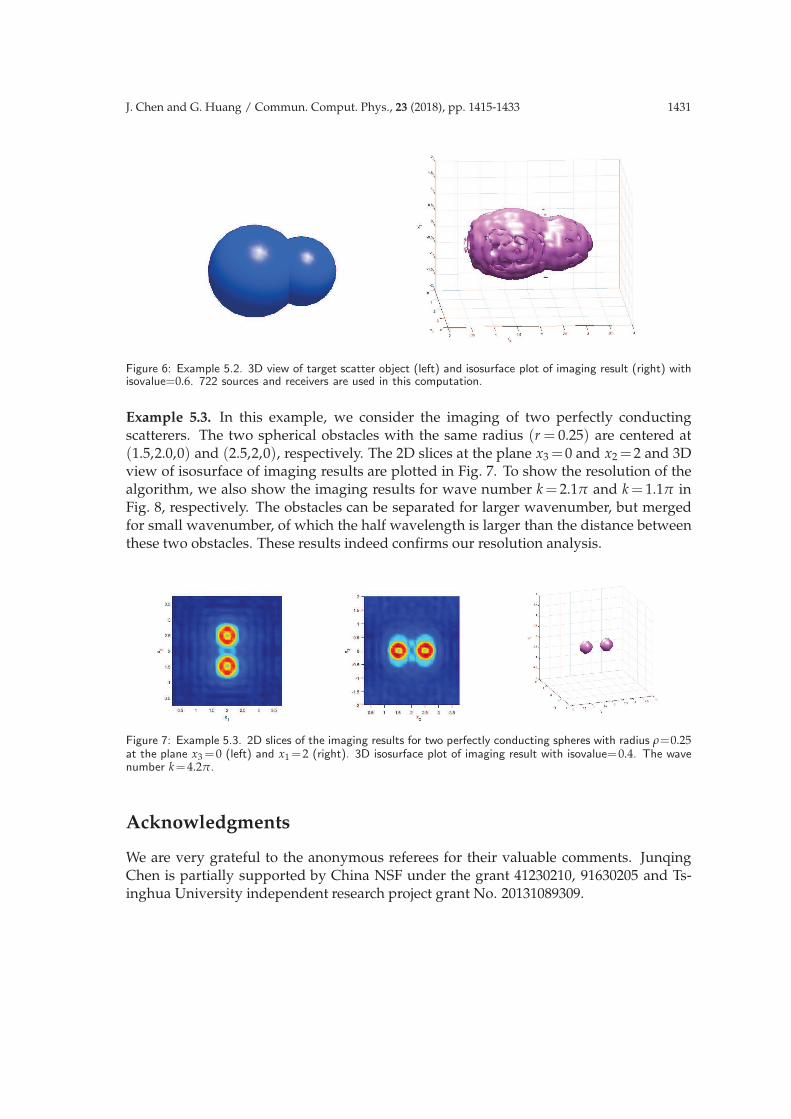
Figure 6: Example 5.2. 3D view of target scatter object (left) and isosurface plot of imaging result (right) withisovalue=0.6. 722 sources and receivers are used in this computation.

Example 5.3. In this example, we consider the imaging of two perfectly conductingscatterers. The two spherical obstacles with the same radius (r = 0.25) are centered at(1.5,2.0,0) and (2.5,2,0), respectively. The 2D slices at the plane x3 =0 and x2=2 and 3Dview of isosurface of imaging results are plotted in Fig. 7. To show the resolution of thealgorithm, we also show the imaging results for wave number k= 2.1π and k= 1.1π inFig. 8, respectively. The obstacles can be separated for larger wavenumber, but mergedfor small wavenumber, of which the half wavelength is larger than the distance betweenthese two obstacles. These results indeed confirms our resolution analysis.

Figure 7: Example 5.3. 2D slices of the imaging results for two perfectly conducting spheres with radius ρ=0.25at the plane x3 =0 (left) and x1=2 (right). 3D isosurface plot of imaging result with isovalue=0.4. The wavenumber k=4.2π.

Acknowledgments

We are very grateful to the anonymous referees for their valuable comments. JunqingChen is partially supported by China NSF under the grant 41230210, 91630205 and Ts-inghua University independent research project grant No. 20131089309.


Figure 8: The imaging results for two perfectly conducting spheres with radius ρ=0.25.The upper two pictures

are imaging results alone the x1−x2 and x2−x3 plane centered at (2,2,0) with k=2.1π (λ= 22.1 ). The lower two

pictures are the imaging results alone the x1−x2 and x2−x3 plane centered at (2,2,0) with k=1.05π (λ= 21.05 ).

References

[1] P. R. Amestoy, I. S. Duff, J. Koster and J. -Y. L’Excellent, A fully asynchronous multifrontal solverusing distributed dynamic scheduling, SIAM Journal of Matrix Analyisi and Applications, Vol23, No. 1(2001), pp 15-41

[2] H. Ammari, E. Iakovleva, D. Lesselier, and G. Perrusson, Music-type Electromagnetic Imagingof a Collection of Small Three-dimensional Inclusions, SIAM J. Sci. Comput. 29 (2007), pp 674-709.

[3] T. Arens, D. Gintides, and A. Lechleiter, Direct and inverse medium scattering in a three-dimensional homogeneous planar waveguide, SIAM J. Appl. Math., 71 (2011), pp. 753-772.

[4] A.J. Berkhout, Seismic Migration: Imaging of Acoustic Energy by Wave Field Extrapolation,Elsevier, New York, 1984.

[5] N. Bleistein, J. Cohen, and J. Stockwell, Mathematics of Multidimensional Seismic Imaging,Migration, and Inversion, Springer, New York, 2001.

[6] L. BOURGEOIS AND E. LUNEVILLE, The linear sampling method in a waveguide: a modal formula-tion, Inverse Problems, 24 (2008), pp. 1-20.

[7] M. Bruhl, M. Hanke and M. Vogelius, A direct impedance tomography algorithm for locating small


inhomogeneities, Numer. Math. 93(2003), pp. 635C54,[8] J. Chen and Z. Chen, An adaptive perfectly matched layer technique for 3-D time-harmonic electro-

magnetic scattering problems, Math. Comp., 77 (2008), pp. 673-698.[9] J. Chen, Z. Chen, and G. Huang, Reverse time migration for extended obstacles: acoustic waves,

Inverse Problems, 29 (2013), 085005 (17pp).[10] J. Chen, Z. Chen, and G. Huang, Reverse time migration for extended obstacles: electromagnetic

waves, Inverse Problems, 29 (2013), 085006 (17pp).[11] Z. Chen and G. Huang, Reverse time migration for reconstructing extended obstacles in planar

acoustic waveguides, Sci. China Math., 58 (2015), pp. 1811-1834.[12] W.C. Chew, Waves and Fields in Inhomogeneous Media, Van Nodtrand Reimhold, New

York, 1990.[13] J.F. Claerbout, Imaging the Earth’s Interior, Blackwell Scientific Publication, Oxford, 1985.[14] D. Colton and A. Kirsch, A simple method for solving inverse scattering problems in the resonance

region, Inverse Problems 12(1996), pp. 383C393.[15] D. Colton and R. Kress, Inverse Acoustic and Electromagnetic Scattering Theory, 2nd ed.,

vol. 93 of Applied Mathematical Sciences, Springer-Verlag, Berlin, 1998.[16] A. Kirsch, Characterization of the shape of a scattering obstacle using the spectral data of the far field

operator, Inverse Problems 14(1998), pp. 1489C1512.[17] S. Dediu and J. R. McLaughlin, Recovering inhomogeneities in a waveguide using eigensystem

decomposition, Inverse Problems, 22 (2006), pp. 1227-1246.[18] K. Ito, B. Jin and J. Zou, A direct sampling method for inverse electromagnetic medium scattering.

Inverse Problems 29 (2013), 095018.[19] X. Liu, A novel sampling method for multiple multiscale targets from scattering amplitudes at a fixed

frequency, arXiv:1701.00537[20] X. Liu, B. Zhang, Recent progress on the factorization method for inverse acoustic scattering prob-

lems (in Chinese). Sci Sin Math, 2015, 45: 873-890[21] A. S. Ilinsky and Yu. G. Smirnov, Electromagnetic Wave Diffraction by Conducting Screens,

VSP, Utrecht, The Netherlands, 1998.[22] J. Schoberl: ”NETGEN - An advancing front 2D/3D-mesh generator based on abstract

rules.” Computing and Visualization in Science, 1(1), pages 41-52, 1997.[23] E. Kilic, F. Akleman, and A. Yapar, Contrast source inversion technique for the reconstruction

of 3D inhomogeneous materials loaded in a rectangular waveguide, Inverse Problems, 27 (2011),105002 (14pp).

[24] E. Kilic, F. Akleman, B. Esen, and et al., 3-D imaging of inhomogeneous materials moaded in atectangular waveguide, IEEE Trans. on Microwave and Technique, 58 (2010), pp. 1290-1296.

[25] K. Kobayashi, Y. Shestopalov, and Y. Smirnov, Investigation of electromagnetic diffraction by adielectric body in a waveguide using the method of volume singular integral equation, SIAM J. Appl.Math., 70 (2009), pp. 969-983.

[26] PHG, Parallel Hierarchical Grid, available online at http://lsec.cc.ac.cn/phg/.[27] Y. Shestopalov and Y. Smirnov, Determination of permittivity of an inhomogeneous dielectric body

in a waveguide, Inverse Problems, 27 (2011), 095010 (12pp).[28] J. SUN AND C. ZHENG, Reconstruction of obstacles embedded in waveguides, Contemporary

Mathematics, 586 (2013), pp. 341-350.[29] C. TSOGKA, D.A. MITSOUDIS, AND S. PAPADIMITROPOULOS, Selective imaging of extended

relectors in two-dimensional waveguides, SIAM J. Imaging Sci., 6 (2013), pp. 2714-2739.[30] Y. XU, C. MAWATA, AND W. LIN, Generalized dual space indicator method for underwater imag-

ing, Inverse Problems, 16 (2000), pp. 1761-1776.

ADirectImagingMethodforInverseElectromagnetic … Scattering Problem in Rectangular Waveguide...

Documents

Transcript of ADirectImagingMethodforInverseElectromagnetic … Scattering Problem in Rectangular Waveguide...