Adaptive Numerical Solution

of MFS Systems

Robert Schaback

February 8, 2008

Dedicated to Professor Graeme Fairweatheron the occasion of his 65th birthday

Abstract

The linear systems arising from MFS calculations share certain nu-merical effects with other systems involving radial basis functions.These effects concern approximation error and stability, which areclosely related, and they can already be studied for simple interpo-lation problems without PDEs. In MFS calculations, they cruciallydepend on the position and density of the source points and the col-location points. In turn, the choice of these points must depend onthe smoothness and possible singularities of the solution. This contri-bution provides an adaptive method which chooses good source pointsautomatically. A series of examples shows that the adaptive choice ofsource points follows the theoretical predictions quite well.

1 Introduction

The Method of Fundamental Solutions (MFS) solves a homogeneousboundary value problem via approximation of the boundary data bytraces of fundamental solutions centered at source points outside thedomain in question. The method has been used extensively in recentyears, and there are excellent surveys [6, 8, 5]. However, this contri-bution focuses on the linear systems arising in MFS calculations andignores applications in engineering and science. Since our observationswill easily generalize to other cases, we keep the presentation and theexamples simple by restricting ourselves to the homogeneous Poissonproblem

∆u = 0 in Ω ⊂ IR2

u = ϕ on Γ := ∂Ω(1)

1

with the Laplace operator. In this case, the fundamental solution (upto a multiplicative constant) is the singular radial kernel function

Φ(x, y) := log ‖x − y‖2

2, x, y ∈ IR2.

The source points will be taken from a curve Σ outside Ω which is oftencalled the “fictitious” boundary. In particular, users normally chooseN points y1, . . . , yN ∈ Σ and take linear combinations

s(x) :=

N∑

j=1

αj log ‖x − yj‖2

2, x ∈ Ω (2)

of fundamental solutions as trial functions being homogeneous solu-tions of the Laplacian, i.e. harmonic functions. Of course, other homo-geneous solutions can also enrich the trial space, and there are plenty ofsuch possibilities, including harmonic polynomials. Methods like thisdate back to Trefftz [16] in much more general form, and are currentlyrevived under the name of boundary knot methods [4].

2 Error Bounds

Whatever homogeneous solutions the trial functions s are composed of,the maximum principle will under mild assumptions on the regularityof the domain and the boundary data [11] imply that the true solutionu and the trial approximation s satisfy the error bound

‖u − s‖∞,Ω ≤ ‖u − s‖∞,∂Ω.

This means that users only have to worry about the L∞ approximationerror on the boundary. If a fixed space of general linear combinations

s(x) :=

N∑

j=1

αjsj(x), x ∈ Ω

of smooth homogeneous solutions sj are admitted, the natural numeri-cal approach induced by the Maximum Principle would be to minimizethe L∞ norm of the error on the boundary. This is a semi–infinite lin-ear optimization problem

Minimize η

−η ≤ ϕ(x) −

N∑

j=1

αjsj(x) ≤ η, x ∈ Γ(3)

with N + 1 variables η, α1, . . . , αn and infinitely many affine–linearconstraints. The literature on optimization deals with such problems[10, 9], but in many cases it suffices to come up with a cheap butsuboptimal approximation. We shall focus on this situation and giveexamples later.

2

3 Linear Systems

In particular, users often try to get away with picking N collocation

points x1, . . . , xN on the boundary Γ and setting up an N × N linearsystem

N∑

j=1

αjsj(xk) = ϕ(xk), 1 ≤ k ≤ N (4)

for interpolation at these points. This works well in many cases, butthe main theoretical problem with such systems is that the coefficientmatrix with entries sj(xk) may be singular. This clearly occurs forN > 1 and the MFS, because the determinant of the N × N systemwith matrix entries

sj(xk) = log ‖yj − xk‖2

2, 1 ≤ j, k ≤ N

will be a smooth function of the source points yj, and swapping twosource points will change the sign of the determinant. Thus there areplenty of configurations of source and test points where the system isnecessarily singular. Confining source points to curves may help in 2Dcases, but not in 3D if source points are restricted to surfaces.

Consequently, it does not make any sense to head for theoremsproving nonsingularity of the above systems. The same holds for otherunsymmetric collocation–type techniques like the one introduced byE. Kansa [12, 13] for general PDE problems in strong form, or themeshless local Petrov–Galerkin method of S.N. Atluri and collabora-tors [1, 2].

Instead, systems like (4) should not be expected to be solvableexactly. In view of the maximum principle and the semi–infinite opti-mization problem (3) one can take many more collocation points thansource points and solve the overdetermined linear system

N∑

j=1

αjsj(xk) = ϕ(xk), 1 ≤ k ≤ M ≥ N (5)

approximatively, e.g. by a standard least–squares solver. We shallfocus on such systems from now on.

4 Choice of Test and Collocation Points

If a good linear combination s of the form (2) is found by any methodwhatsoever, users will check the maximum boundary error ‖ϕ− s‖∞,Γ

by evaluating the error in sufficiently many test points on the boundary.Though this test also needs a thorough mathematical analysis in orderto be safe, we ignore it here. We just remark that users will need very

3

many test points in case of steep gradients of the trial functions, andthis inevitably occurs if the MFS is used with source points close tothe boundary. Adding more test points still is computationally cheapif N is not too large, and most users will be satisfied with a simple plotof the boundary errors evaluated at test points guaranteeing graphicaccuracy, i.e. at most 1000 points per plot. We shall use this rule–of–thumb in later examples.

Choosing M collocation points for setting up the system (4) is some-what more difficult, but it will always stabilize the system if morepoints are taken. Independent of the choice of trial functions, userscan repeat the calculation with more or other collocation points, ifthey are not satisfied with the first result. This is a simple way ofintroducing adaptivity into the numerical solution strategy:

Adaptivity of Testing:If the evaluation of the boundary error on certain test pointsyields values that are intolerably large, take these test points ascollocation points and repeat the calculation.

As long as the trial space S is not changed, this can improve the results,but if the trial space is poorly chosen, the final boundary error cannotbe less than

infs∈S

‖ϕ − s‖∞,Γ (6)

no matter how collocation and testing is done and how many pointsare used.

But there is another argument that needs consideration. If thelinear optimization problem (3) is solved for a large but finite subset Γ0

of the boundary instead of the full boundary, the Karush–Kuhn–Tuckerconditions applied to the dual reformulation [3] of a linear minimaxproblem will imply that there is a subset Γ1 of Γ0 consisting of at mostN + 1 points such that

infs∈S

‖ϕ − s‖∞,Γ0= inf

s∈S‖ϕ − s‖∞,Γ1

.

This is related to the notion of support vectors in support vector ma-chines, and it has the following implication:

Reducibility of collocation points:If a system (4) with M >> N has a good approximate solution,it even has a good approximate solution determined already bya subset of at most N + 1 collocation points.

Unfortunately, these collocation points are not known beforehand, butusers should be aware of the fact that a large system with a good ap-proximate solution will have a much smaller subsystem with an equallygood solution. This fact will reappear later, and we shall provide ex-amples.

4

5 Choice of Trial Space

The lower bound (6) for the achievable boundary error reveals thatthe main design problem consists in picking good trial functions, or,in case of the MFS, in picking good source points.

Let us postpone the MFS for a while. Users can take all homo-geneous solutions as trial functions, and this will work well in certainexamples we shall look at later. For the Laplace operator in 2D, thereal part of any differentiable function of a complex variable will be har-monic and can serve as a possible trial function. The standard funda-mental solution just is a special case of a real part of a complex functionwith a singularity, but there are many others without singularities, e.g.harmonic polynomials or entire functions like f(x, y) := exp(y) cos(x).

How to choose? We shall later let an algorithm decide adaptively,but there is a general though trivial rule:

Take trial functions with similar analytic properties as the ex-pected solution. In particular, be careful when the solution or oneof its derivatives will necessarily have singularities somewhere.

6 Harmonic Polynomials

We explain this first for the case of using harmonic polynomials. Ifthe solution u of the given Poisson problem is itself a real part of afunction of a complex variable without singularities anywhere, it canbe well approximated by harmonic polynomials on any curve, namelyby the real part of its partial sums of its power series. The shape of thedomain does not matter at all, and the background PDE problem iscompletely irrelevant because we only have to recover a partial powerseries. A full power series of an analytic function is determined byvalues on any countable set with an accumulation point, and thusrecovery of globally harmonic functions from point evaluation datawill work almost anywhere.

By analogy to certain theorems on polynomial approximations toanalytic functions [7], the rate of approximation can be expected tobe spectral, i.e. the error should behave like Cλn → ∞ as a functionof the degree n of the harmonic polynomials used, and λ > 0 can bearbitrarily small. Then the choice of harmonic polynomials should besuperior to all choices of fundamental solutions. In many engineeringapplications where MFS users report that source points of the MFStaken far away from the domain work best, the special examples usuallyhave solutions without singularities anywhere, but users tend to ignorethat harmonic polynomials will do even better in such situations.

If the solution, when viewed as a global function, is still harmonicbut has a singularity at a positive distance to the boundary Γ, the rate

5

of approximation will again be like Cλn → ∞, but with λ < 1 nowbeing bounded below, and related to the distance of the singularity tothe boundary, with λ → 1 if the singularity moves towards the bound-ary. Again, the shape and smoothness of the boundary is irrelevant.The crucial quantity is the distance of the closest singularity of the so-lution from the boundary, when the solution is extended harmonicallyas far as possible. Again, this case is hard to beat by the MFS, if thesingularity is sufficiently far away from the domain.

The situation gets serious if the solution or one of its derivativeshas a singularity directly on the boundary Γ. Note that this case oc-curs whenever the boundary data, however smooth, are given by afunction which is not itself harmonic. In such a case, the rate of ap-proximation of boundary values by harmonic polynomials can be verypoor, depending on the smoothness of the solution when restricted tothe boundary. The upshot of this discussion of harmonic polynomialsis that the MFS makes sense only if the boundary data come froma non–harmonic function or if there is no harmonic extension of thesolution without singularities close to the boundary. Users working inapplication areas do not seem to be aware of this fact.

7 Rescaling Fundamental Solutions

Before we go over to the problem of choosing good source points for theMFS, let us consider the case of far–away source points y ∈ IR2 whilethe evaluation of a fundamental solution log ‖x−y‖2

2 is at x ∈ IR2 witha relatively small value of ‖x‖2. In such cases, the functions log ‖x−y‖2

2

will not differ much if y varies, and consequently the resulting matrixgets a bad condition. But we can rewrite the function for large ‖y‖2 6= 0as

log ‖x − y‖22 = log

(

‖x‖22 − 2(x, y)2 + ‖y‖2

2

)

= log

(

‖y‖2

2

(

‖x‖22

‖y‖22

− 2

(

x,y

‖y‖22

)

2

+ 1

))

= log ‖y‖22 + log

(

1 +

(

‖x‖22

‖y‖22

− 2

(

x,y

‖y‖22

)

2

))

.

If we use the expansion

log(1 + z) =

∞∑

j=1

(−1)j−1zj

j

6

for |z| < 1, we get for sufficiently large ‖y‖2 the expansion

log ‖x − y‖22 − log ‖y‖2

2

= log

(

1 +

(

‖x‖22

‖y‖22

− 2

(

x,y

‖y‖22

)

2

))

=

∞∑

j=1

(−1)j−1

j

(

‖x‖22

‖y‖22

− 2

(

x,y

‖y‖22

)

2

)j

=

∞∑

j=1

(−1)j−1

j

j∑

m=0

(

j

m

)(

‖x‖22

‖y‖22

)j−m(

−2

(

x,y

‖y‖22

)

2

)m

=

∞∑

j=1

(−1)j−1

j

j∑

m=0

(

j

m

)

1

‖y‖2j−m2

‖x‖2j−2m2

(

−2

(

x,y

‖y‖2

)

2

)m

=

∞∑

k=1

1

‖y‖k2

∑

k/2≤j≤k

(−1)j−1

j[

j∑

m=0

(

j

2j − k

)

‖x‖2k−2j2

(

−2

(

x,y

‖y‖2

)

2

)2j−k]

=:

∞∑

k=1

1

‖y‖k2

pk(x, y)

of the fundamental solution at y into harmonic polynomials

pk(x, y) :=∑

k/2≤j≤k

(−1)j−1

j

j∑

m=0

(

j

2j − k

)

‖x‖2k−2j2

(

−2

(

x,y

‖y‖2

)

2

)2j−k

with respect to x of degree k. If we push the source point y to infinityby writing it as y = rz for large r > 0 and fixed z ∈ IR2 with ‖z‖2 = 1,we get

log ‖x − rz‖22 = 2 log r +

∞∑

k=1

1

rkpk(x, z)

and this is something like a “far field expansion” of the fundamen-tal solution. Note that z and r are considered to be fixed, and thususers are strongly advised to include constants into the space of trialfunctions in order to cope with the 2 log r term.

Now let us look at the span of fundamental solutions based onpoints yj = rzj on a circle of radius r for large r. We want to findfunctions which are in the span when taking the limit r → ∞, and wecall this the “asymptotic span”. The linear combinations are

sr(x) =

N∑

j=1

αj(r)

(

2 log r +

∞∑

k=1

1

rkpk(x, zj)

)

= 2 log rN∑

j=1

αj(r) +∞∑

k=1

1

rk

N∑

j=1

αj(r)pk(x, zj)

7

and thus have specific expansions in terms of harmonic polynomials.If constants are not added to the span, and if the MFS works at allfor large r in a specific case, the sum of the coefficients αj(r) will tendto zero for r → ∞ while the coefficients themselves cannot stay allbounded. In all “pure MFS” examples with far-away source points,the sum of coefficients will always be close to zero while the sum of theabsolute values will be extremely large.

To avoid computational crimes, we now add the constant 1 to thespan of trial functions and use a coefficient α0 for it. Then we have aspan of

sr(x) = 1

α0(r) + 2 log r

N∑

j=1

αj(r)

+

∞∑

k=1

1

rk

N∑

j=1

αj(r)pk(x, zj)

which we can analyze somewhat easier. We have the constants in thespan, of course, but for arbitrary α1(r), . . . , αN (r) we can always set

α0(r) := −2 log r

N∑

j=1

αj(r)

to cancel the first term. Now rsr(x) must be in the span, and thisasymptotically is in the span of the p1(x, zj), 1 ≤ j ≤ N , whichnecessarily is a subspace V1 of the linear polynomials. To proceedinductively, we now look at the subspace A1 of coefficient vectors α ∈IRN with

N∑

j=1

αjp1(x, zj) = 0.

If we take a vector α ∈ A1 and form the functions r2sr(x), we findthat the aymptotic span of the fundamental solutions contains thepolynomial space

V2 :=

N∑

j=1

αjp2(x, zj) : α ∈ A1

of maximally second–degree polynomials. Inductively we can defineA0 := IRN and

Am :=

α ∈ IRN :N∑

j=1

αjpi(x, zj) = 0, 1 ≤ i ≤ m

for all m ≥ 1 and use it for defining a space

Vm :=

N∑

j=1

αjpm(x, zj) : α ∈ Am−1

8

of polynomials of degree at most m. The spaces Am form an inclusionchain

RN = A0 ⊇ A1 ⊇ A2 ⊇ · · ·

and if we take an appropriate orthogonal basis for that chain, we get

Theorem 1 The asymptotic span for r → ∞ of fundamental solutions

with source points of the form yj = rzj for fixed points zj on the unit

circle is a space of harmonic polynomials spanned by constants and the

union of all Vm. 2

Unfortunately, it seems to be difficult to calculate the dimension ofthat space, because it will depend on the number and the geometry ofthe points zj .

The upshot of all of this is that the MFS for far–away source points,if it works at all, is asymptotically nothing else than a fit of the bound-ary data by specific harmonic polynomials. Thus the MFS should notbe used at all for far–away source points, but rather be replaced byuse of harmonic polynomials. For this reason, we do not elaboratethe above argument any further, though it would result in a way ofpreconditioning MFS matrices for far–away points. It does not makesense to precondition a matrix one should not use.

However, a rather primitive but still somewhat useful change ofbasis induced by the above argument is to add constants to the MFSspan and replace the fundamental solution at y 6= 0 by

(

log ‖x − y‖2

2 − log ‖y‖2

2

)

‖y‖2

behaving like a linear polynomial in x when y is far away from x. A fullpreconditioning will use such basis changes plus coefficient vectors froman orthogonal basis of IRN which is compatible with the chain of theAm spaces. Details can be worked out similarly to [19]. As an aside,we remark that it is no problem to replace the standard fundamentalsolutions by rational trial functions arising when taking derivatives oflog ‖x − ry‖2

2 with respect to r.Finally, we present an example supporting the results of this and

the previous section. In Figure 1 we show the L∞ error ǫ∞(r) on thefull circle when we recover the harmonic function f(x, y) = ex cos(y)from boundary values only on a half circle. We collocate at 100 testpoints on the right half unit circle, using 20 source points on the righthalf circle of radius r. We stopped the calculation when the numeri-cal rank of the 100 × 20 collocation matrix, as given by MATLAB c©

was less than 20, and this occurred for r ≈ 5.5 already. The error de-creases nicely with increasing r, because the setting converges towardsharmonic polynomials for r → ∞, as was shown in this section, andsince the discussion in the previous section showed that recovery byharmonic polynomials should work on any arc.

9

2 2.5 3 3.5 4 4.5 5 5.5 610

−3

10−2

10−1

100

Radius for sources

L ∞ E

rror

Figure 1: L∞ error as function of r

8 Choice of Source Points

It should be clear by now that a good placement of source pointswill crucially depend on the distance of the closest singularity arisingwhen extending the solution harmonically outside the domain. In manycases, the user normally does not have this information, but there area few guidelines.

We start by an upside–down argument. If the MFS works for suf-ficiently many source points on a fixed curve Σ, and if the results aregetting better when taking more source points, the solution will havea harmonic extension up to Σ, because the MFS constructs it. But ifthere necessarily is a singularity inside Σ for some reason or other, theMFS cannot work satisfactorily on Σ.

We now have to find a–priori indicators for singularities close to theboundary. The first and simplest case arises when the known boundarydata are such that there is no C∞ extension locally into R2. Thisalways happens if the boundary data are not C∞ on smooth partsof the boundary. If users know where the “boundary points of datanonsmoothness” are, source points should be placed close to those.Unfortunately, there currently is no general way to guess the type ofsingularity beforehand, even if the position is known. Thus this caseusually must be handled experimentally.

A second and partially independent case arises for incoming cornersof the domain. Even if the boundary data have a C∞ extension toIR2, e.g. if they are non–harmonic polynomials, users must expecta singularity at the boundary, but the type of singularity is known,depending on the boundary angle. Again, users should either add thecorrect type of singularity or place source points close to corners insuch cases. But the situation is different if the data come from anextendable harmonic function, even if corners are present. Then theMFS can ignore the corners. Note that MFS examples on domainswith corners are useless as long as they consider specific boundary

10

data which are values of functions with a harmonic extension.Finally, the convergence rate of the MFS when adding more and

more source points will be strongly influenced by the smoothness ofboth the data function and the MFS trial functions on the bound-ary. Approximation theory proves in many situations that conver-gence rates are completely controlled by the minimal smoothness ofthe data function and the trial functions. Thus smooth boundary dataon smooth boundaries will lead to good convergence rates improvingwith the smoothness properties. If source points can be kept at afixed positive minimal distance from the boundary (this requires thesolution to have a harmonic extension), then the trial functions are an-alytic and the convergence rate will be completely determined by thesmoothness of the data on the boundary. But then the approximationby harmonic polynomials on the boundary will also have a good con-vergence rate depending on the smoothness of the boundary data, andit is not easy to predict superiority of the MFS over approximation byharmonic polynomials.

If singularities of derivatives are on the boundary or if there are in-coming corners, the convergence rate of approximation of the boundarydata by harmonic polynomials will deteriorate seriously, and the MFScan be competitive by placing source points closer and closer to thesingularities. A general rule is not known, but there are certain adap-tive techniques [18, 14, 15, 6] to handle this case. We shall provide asimple adaptive method in the next section.

9 Greedy Adaptive Techniques

Overdetermined systems like (5) can be approximately solved by astep–wise adaptive techniques even if they are huge. We applied themethod of [17] to MFS problems, but it turned out to be less stablethan the algorithm we describe now, because the previous one did notkeep all collocation points under control.

The basic idea can be formulated independent of the MFS in termsof solving a linear unsymmetric over– or underdetermined m×n systemof the form Ax = b. The goal is to pick useful columns of the m × nmatrix A in a data–dependent way without cutting the number of rowsdown. This is also done by any reasonable solution algorithm, e.g. bythe backslash operator in MATLAB c©, and we shall present exampleslater. However, standard QR routines do not account for the right–hand side b, and they do not stop early when only a few columns ofthe matrix suffice to reproduce the right–hand side with small error.To maintain stability, we use orthogonal transformations like in anyQR decomposition, but we make the choice of columns dependent onthe right–hand side.

11

In short, our adaptive algorithm for selecting good columns worksas follows:

1. Pick the column of A whose multiples approximate b best.

2. Then transform the problem to the space orthogonal to that col-umn and repeat.

If the algorithm has selected a number of columns this way, take thiscolumn selection for a trial space and use your algorithm of choice forsolving the given problem on that trial space. For instance, in MFSapplications one can use L∞ minimization of boundary errors after theselection process has provided a small set of useful source points.

The actual implementation of the algorithm needs some furtherexplanation. Approximation of b by multiples of a single nonzero vector

a is optimal in L2, if the error vector has the form b − a · bT aaT a , and its

squared norm then takes the minimal possible value

‖b‖2

2 −(bT a)2

‖a‖22

.

If we denote the columns of A by a1, . . . , an, we thus can implementStep 1 by taking the maximum of

(bT aj)2

‖aj‖22

, 1 ≤ j ≤ n, ‖aj‖2 6= 0

to pick the best column for approximation of b. If we denote thiscolumn by u, we form the normalized vector v := u/‖u‖2 and transformboth A and b into

A1 := A − v(vT A)b1 := b − v(vT b)

to let both b1 and the columns of A1 be orthogonal to u and v. Thenew matrix has a zero column where once was u. To avoid roundoffproblems, we insert exact zeros there, but we do not delete the zerocolumn in order to avoid unnecessary storage transformations. Instead,we store the column index of u for later use and proceed. The followingsteps will always automatically ignore the columns we already picked.Note that we do not care for the approximate solution of the systemand about accumulation of roundoff during the transformations. TheL2 norms of the vectors b, b1, . . . will necessarily decrease, and this canbe used for stopping the algorithm. Going for a strong error reductionwill finally use the full matrix, while users can get away with just afew columns and a very simple numerical solution if they admit largererrors. A MATLAB c© package is available from the author.

Application of this technique to MFS calculations is particularlyappealing in cases where the user lets the algorithm decide which trial

12

function to choose. One can offer harmonic polynomials up to a fixeddegree and plenty of fundamental solutions at different distances to theboundary, and the algorithm will pick suitable ones without knowingbackground mathematics like harmonic extendibility of the solution.Running the algorithm several times will provide the user with in-formation about hazardous places at the boundary, and the user canoffer refined choices of source points close to these when preparing thenext run. The actual calculation of the solution is done after columnselection in order to keep the accumulated errors small.

10 Examples

To illustrate the mathematical issues of the previous sections, we nowprovide a series of examples, but we have to explain the notation in thetables and figures first. Following (4), the number of collocation pointswill be M , and N will denote the number of source points offered tothe algorithm. If only a smaller subset of source points is actually usedfor the calculation, we use n ≤ N . Similarly, K denotes the number ofharmonic polynomials included into the trial space, and k stands for thenumber actually arising in the solution. For approximate evaluation ofthe L∞ norm ǫ∞ of the error on the boundary we use max(1000, 5∗N)points for graphic accuracy. The number M of collocation points isalways defined as 1 + max(200, 2N + 2K). The approximate solutionof the system will be done by algorithms labeled as

L2: the MATLAB c© backslash operator, i.e. a standard least–squaressolver with internal selection of columns,

A2: the same as above, but applied to the reduced matrix after adap-tive column selection along the lines of the previous section,

A∞: an L∞ linear optimizer applied to the same adaptively reducedmatrix.

Note that the solution algorithm will have quite some influence on thefinal error and the number of nonzero solution coefficients. The L2solver always exploits maximal machine accuracy, while our adaptivesolvers A2 and A∞ are tuned for a compromise between error andcomplexity.

We denote the L∞ error on our test points as ǫ∞. It is debatableto use the RMSE error measure at all, because the Maximum Principleis guiding the error behavior, but we also include it as ǫ2. The curveswe use for boundaries or source points consist of circles Cr with radiusr around zero, or they are obtained from a polar coordinate represen-tation of the standard boundary B0 by adding a distance h to get asource boundary Bh at polar distance h.

13

The first example in Table 1 concerns a more or less trivial casewhere the data come from a globally harmonic function f(x, y) =exp(x) cos(y) which is the real part of the entire complex functionexp(z) = exp(x + iy). The real part of the power series of exp(z)yields a sequence of perfect approximations by harmonic polynomialson each domain whatsoever, and the recovery by collocation via har-monic polynomials even works on open arcs anywhere. As expected,the MFS cannot outperform harmonic polynomials, independent ofwhere the sources are. The domain is a lemniscate with an incomingcorner as in Figure 2, while the source points are on the circle of radius4 around the origin.

N M K Alg n m k ǫ∞ ǫ2

0 201 25 L2 0 201 13 1.16e-011 7.53e-0120 201 25 A2 0 201 12 1.82e-010 1.18e-0100 201 25 A∞ 0 201 12 1.81e-010 1.18e-010

200 401 0 L2 36 401 0 1.54e-013 6.74e-014200 401 0 A2 25 401 0 3.54e-009 1.90e-009200 401 0 A∞ 28 401 0 5.88e-007 2.04e-007200 451 25 L2 7 451 22 5.18e-010 1.79e-010200 451 25 A2 1 451 11 5.79e-010 3.73e-010200 451 25 A∞ 1 451 11 7.49e-010 3.89e-010

Table 1: Recovery of harmonic function

−4 −3 −2 −1 0 1 2 3 4

−4

−3

−2

−1

0

1

2

3

4

Figure 2: Lemniscate with source points

The table should be interpreted as follows. The first three linesused no source points at all (N = 0), but M = 201 collocation pointsand allowed K = 25 harmonic polynomials. Only up to k = 13 nonzeropolynomial coefficients were calculated due to the symmetry of the data

14

function, and the recovery quality via the first terms of the power seriesis around 1.0e−10, independent of the algorithm used. This happenedfor all domains tested. But the adaptive algorithms in lines 2 and 3solve only a subproblem with 12 degrees of freedom after picking themost useful harmonic polynomials.

The next three lines are a pure MFS offering 200 source pointson the circle. With the L2 solver, the results are even better thanfor harmonic polynomials, and surprisingly the MATLAB backslashsolver yields only 36 nonzero coefficients, i.e. only 36 source pointswere necessary. The adaptive solvers are satisfied with less accuracy,but also use a simpler approximation by 25 or 28 source points.

The final three lines offered the same 200 source points, but allowedalso 25 harmonic polynomials. All algorithms prefer harmonic poly-nomials over fundamental solutions. This is to be expected, becausethe solution has no finite singularities. The 25 marked source pointsin Figure 2 belong to the situation of the fifth line of Table 1. Theadaptive L2 algorithm picks these 25 source points with no connectionto the domain corner, as is to be expected. However, the error is worsethan for harmonic polynomials in this case.

The L∞ norm of the error using the A∞ solver in line 3 is onlyslightly better than the one from the A2 solver in line 2. It cannot beworse because they use the same trial space. However, in some of thelater cases, the A∞ algorithm, after starting from the same trial spaceas the A2 algorithm, is less stable and often ends prematurely with alarger L∞ error than the A2 solver. Future work should add a moresophisticated L∞ solver.

In Table 2 we present the same situation, but with boundary datagiven by the function x2y3. This is still smooth, but the domain hasan incoming corner causing problems.

N M K Alg n m k L∞ L2

0 201 25 L2 0 201 12 1.17e-003 3.38e-0040 201 25 A2 0 201 12 1.17e-003 3.38e-0040 201 25 A∞ 0 14 12 9.28e-004 6.48e-004

200 401 0 L2 36 401 0 9.41e-004 2.38e-004200 401 0 A2 31 401 0 1.04e-003 2.78e-004200 401 0 A∞ 32 34 0 1.31e-003 8.30e-004200 451 25 L2 7 451 24 1.02e-003 2.72e-004200 451 25 A2 0 451 12 1.17e-003 3.38e-004200 451 25 A∞ 0 26 12 9.15e-004 6.46e-004

Table 2: Smooth boundary data on lemniscate, source points on circle

15

With source points on the circle, none of the methods outperformsharmonic polynomials seriously.

To demonstrate that the incoming corner is the culprit, we replacethe lemniscate now by the unit circle and get Table 3. Again, harmonicpolynomials do best. We now go back to the lemniscate, but place the

N M K Alg n m k L∞ L2

0 201 25 L2 0 201 3 1.67e-016 4.61e-0170 201 25 A2 0 201 3 2.08e-016 6.84e-0170 201 25 A∞ 0 201 3 1.42e-014 1.00e-014

200 401 0 L2 34 401 0 1.90e-008 9.64e-009200 401 0 A2 33 401 0 3.31e-009 1.48e-009200 401 0 A∞ 33 274 0 7.56e-006 3.38e-006200 451 25 L2 17 451 11 6.47e-010 3.47e-010200 451 25 A2 0 451 3 2.36e-016 9.79e-017200 451 25 A∞ 0 451 3 7.31e-011 4.79e-011

Table 3: Smooth boundary data on circle

source points at a polar radial distance of 0.2 outside the boundary(i.e. we calculate them by adding 0.2 to the radius of boundary pointsin polar coordinates). This gives Table 4 and should be compared toTable 2. The results are not better than for sources on the circle, but

N M K Alg n m k L∞ L2

0 201 25 L2 0 201 12 1.17e-003 3.38e-0040 201 25 A2 0 201 12 1.17e-003 3.38e-0040 201 25 A∞ 0 14 12 9.28e-004 6.48e-004

200 401 0 L2 200 401 0 3.09e-004 4.75e-005200 401 0 A2 140 401 0 3.09e-004 4.75e-005200 401 0 A∞ 140 386 0 3.66e-004 8.18e-005200 451 25 L2 193 451 9 2.90e-004 4.32e-005200 451 25 A2 104 451 13 3.09e-004 4.75e-005200 451 25 A∞ 104 119 13 4.82e-004 1.28e-004

Table 4: Smooth boundary data on lemniscate, source points at 0.2

maybe the sources are not close enough. Thus we go for a distanceof 0.02 in Table 5, and Figure 3 shows the source point distribution(circles, while the offered but unused source points are small dots) forthe A2 technique in the eighth line of Table 5. Note that the source

16

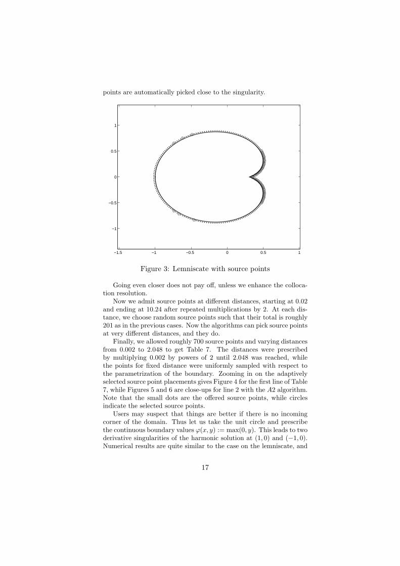
points are automatically picked close to the singularity.

−1.5 −1 −0.5 0 0.5 1

−1

−0.5

0

0.5

1

Figure 3: Lemniscate with source points

Going even closer does not pay off, unless we enhance the colloca-tion resolution.

Now we admit source points at different distances, starting at 0.02and ending at 10.24 after repeated multiplications by 2. At each dis-tance, we choose random source points such that their total is roughly201 as in the previous cases. Now the algorithms can pick source pointsat very different distances, and they do.

Finally, we allowed roughly 700 source points and varying distancesfrom 0.002 to 2.048 to get Table 7. The distances were prescribedby multiplying 0.002 by powers of 2 until 2.048 was reached, whilethe points for fixed distance were uniformly sampled with respect tothe parametrization of the boundary. Zooming in on the adaptivelyselected source point placements gives Figure 4 for the first line of Table7, while Figures 5 and 6 are close-ups for line 2 with the A2 algorithm.Note that the small dots are the offered source points, while circlesindicate the selected source points.

Users may suspect that things are better if there is no incomingcorner of the domain. Thus let us take the unit circle and prescribethe continuous boundary values ϕ(x, y) := max(0, y). This leads to twoderivative singularities of the harmonic solution at (1, 0) and (−1, 0).Numerical results are quite similar to the case on the lemniscate, and

17

N M K Alg n m k L∞ L2

0 201 25 L2 0 201 12 1.17e-003 3.38e-0040 201 25 A2 0 201 12 1.17e-003 3.38e-0040 201 25 A∞ 0 14 12 9.28e-004 6.48e-004

200 401 0 L2 198 401 0 1.16e-004 2.28e-005200 401 0 A2 196 401 0 1.16e-004 2.28e-005200 401 0 A∞ 196 401 0 2.51e-004 9.65e-005200 451 25 L2 198 451 12 1.17e-004 1.09e-005200 451 25 A2 58 451 12 1.17e-004 1.09e-005200 451 25 A∞ 58 450 12 4.32e-004 1.07e-004

Table 5: Smooth boundary data on lemniscate, source points at 0.02

N M K Alg n m k L∞ L2

210 451 25 L2 111 451 21 3.64e-004 5.75e-005210 451 25 A2 50 451 12 3.63e-004 5.75e-005210 451 25 A∞ 50 447 12 6.12e-004 1.45e-004

Table 6: Smooth boundary data on lemniscate, about 200 source points atvarying distances

thus we confine ourselves to offering about 700 source points on circleswith distances 0.002 to 2.048 in Table 8. The L2 solver does notcare about the right–hand side of the system, and thus it does notrealize the two singularities. This is shown in a close–up in Figure 7,while the A2 algorithm (see Figure 8) selects source points close tothe problematic boundary locations. Note that this case is offered 729degrees of freedom and uses maximally 490 of these.

If we drop the MFS completely and offer 751 harmonic polynomialson the circle instead, we get Table 9. Note that this performs slightlybetter than the MFS and uses 377 of the possible degrees of freedom.

N M K Alg n m k L∞ L2

704 1451 25 L2 416 1451 11 7.55e-005 5.31e-006704 1451 25 A2 208 1451 12 6.97e-005 4.93e-006704 1451 25 A∞ 211 1451 12 4.80e-003 6.97e-004

Table 7: Smooth boundary data on lemniscate, about 700 source points atvarying distances

18

−1.5 −1 −0.5 0 0.5 1

−1.5

−1

−0.5

0

0.5

1

1.5

Figure 4: Lemniscate with source points, L2 algorithm

N M K Alg n m k L∞ L2

704 1451 25 L2 471 1451 19 7.69e-004 3.41e-005704 1451 25 A2 350 1451 13 8.13e-004 3.03e-005704 1451 25 A∞ 356 1449 14 6.92e-003 2.01e-003

Table 8: MFS results for max(0, y)

Finally, Table 10 shows how the sum of coefficients and the L1 normof coefficients vary with the radius r of the distance of the source pointsto the boundary. To avoid symmetries, we took the boundary datafunction f(x, y) := max(0, |y|) on the unit circle, offered 200 sourcepoints on a circle of radius r and used 401 collocation points. The so-lution method was the standard backslash L2 solver from MATLAB c©.Note that the increase of condition is counteracted by the solver in avery nice way, using fewer and fewer source points. This effect is evenmore significant when using the A2 or A∞ methods.

19

−1.5 −1 −0.5 0 0.5 1 1.5

−1.5

−1

−0.5

0

0.5

1

1.5

Figure 5: Lemniscate with source points, A2 algorithm

N M K Alg n m k L∞ L2

0 1503 751 L2 0 1503 377 6.67e-004 4.08e-0050 1503 751 A2 0 1503 377 6.67e-004 4.08e-0050 1503 751 A∞ 0 379 377 1.47e-003 1.90e-004

Table 9: Results for max(0, y), harmonic polynomials only

References

[1] S. N. Atluri and T. L. Zhu. A new meshless local Petrov-Galerkin(MLPG) approach in computational mechanics. Computational

Mechanics, 22:117–127, 1998.

[2] S. N. Atluri and T. L. Zhu. A new meshless local Petrov-Galerkin(MLPG) approach to nonlinear problems in computer modelingand simulation. Computer Modeling and Simulation in Engineer-

ing, 3:187–196, 1998.

[3] I. Barrodale and A. Young. Algorithms for best L1 and L∞ linearapproximations on a discrete set. Numer. Math., 8:295–306, 1966.

[4] W. Chen. Boundary knot method for Laplace and biharmonicproblems. In Proc. of the 14th Nordic Seminar on Computational

20

−0.2 0 0.2 0.4 0.6 0.8 1 1.2

−0.8

−0.6

−0.4

−0.2

0

0.2

0.4

0.6

0.8

Figure 6: Lemniscate with source points, A2 algorithm

Mechanics, pages 117–120. Lund, Sweden, 2001.

[5] H.A. Cho, M.A. Golberg, A.S. Muleshkov, and X. Li. Trefftzmethods for time dependent partial differential equations. Com-

puters, Materials, and Continua, 1:1–38, 2004.

[6] G Fairweather and A. Karageorghis. The method of fundamen-tal solution for elliptic boundary value problems. Advances in

Computatonal Mathematics, 9:69–95, 1998.

[7] D. Gaier. Lectures on Complex Approximation. Birkhauser,Boston, 1987.

n r ǫ∞ sum L1 norm

57 1 1.13e-002 2.30e-001 7.23e+00953 2 1.15e-002 1.45e-001 2.09e+01135 4 1.86e-002 9.89e-002 6.44e+00922 8 2.87e-002 7.24e-002 1.56e+01118 16 3.50e-002 5.62e-002 3.33e+00918 32 3.89e-002 4.57e-002 1.62e+012

Table 10: Sums of coefficients as functions of r

21

−1.5 −1 −0.5 0 0.5 1 1.5

−1.5

−1

−0.5

0

0.5

1

1.5

Figure 7: Source points selected by L2 algorithm

[8] M.A. Golberg and C.S. Chen. The method of fundamentalsolutions for potential, Helmholtz and diffusion problems. InM.A. Golberg, editor, Boundary Integral Methods: Numerical and

Mathematical Aspects, pages 103–176. WIT Press, 1998.

[9] R. Hettich and K. O. Kortanek. Semi-infinite programming: the-ory, methods, and applications. SIAM Rev., 35(3):380–429, 1993.

[10] Rainer Hettich and Peter Zencke. Numerische Methoden der

Approximation und semi-infiniten Optimierung. B. G. Teubner,Stuttgart, 1982. Teubner Studienbucher Mathematik. [TeubnerMathematical Textbooks].

[11] Jurgen Jost. Partial differential equations, volume 214 of Graduate

Texts in Mathematics. Springer-Verlag, New York, 2002. Trans-lated and revised from the 1998 German original by the author.

[12] E. J. Kansa. Application of Hardy’s multiquadric interpolation tohydrodynamics. In Proc. 1986 Simul. Conf., Vol. 4, pages 111–117, 1986.

[13] E. J. Kansa. Multiquadrics - a scattered data approximationscheme with applications to computational fluid-dynamics - I:Surface approximation and partial dervative estimates. Comput.

Math. Appl., 19:127–145, 1990.

22

−1.5 −1 −0.5 0 0.5 1 1.5

−1.5

−1

−0.5

0

0.5

1

1.5

Figure 8: Source points selected by A2 algorithm

[14] A. Karageorghis and G. Fairweather. The method of fundamentalsolutions for the solution of nonlinear plane potential problems.IMA Journal of Numerical Analysis, 9:231–242, 1989.

[15] A. Karageorghis and G. Fairweather. The simple layer potentialmethod of fundamental solutions for certain biharmonic problems.International Journal of Numerical Methods in Fluids, 9:1221–1234, 1989.

[16] Zi-Cai Li, Tzon-Tzer Lu, Hung-Tsai Huang, and Alexander H.-D. Cheng. Trefftz, collocation, and other boundary methods—a comparison. Numer. Methods Partial Differential Equations,23(1):93–144, 2007.

[17] L.L. Ling, R. Opfer, and R. Schaback. Results on meshless collo-cation techniques. Engineering Analysis with Boundary Elements,30:247–253, 2006.

[18] R. Mathon and R.L. Johnston. The approximate solution of el-liptic boundary-value problems by fundamental solutions. SIAM

J. Numer. Anal., 14:638–650, 1977.

[19] R. Schaback. Limit problems for interpolation by analytic radialbasis functions. Preprint, to appear in J. of Computational andApplied Mathematics, 2006.

23