Adaptive Geometric Numerical Integration of Mechanical ... · Adaptive Geometric Numerical...
151
Adaptive Geometric Numerical Integration of Mechanical Systems Modin, Klas Published: 2009-01-01 Link to publication Citation for published version (APA): Modin, K. (2009). Adaptive Geometric Numerical Integration of Mechanical Systems Matematikcentrum General rights Copyright and moral rights for the publications made accessible in the public portal are retained by the authors and/or other copyright owners and it is a condition of accessing publications that users recognise and abide by the legal requirements associated with these rights. • Users may download and print one copy of any publication from the public portal for the purpose of private study or research. • You may not further distribute the material or use it for any profit-making activity or commercial gain • You may freely distribute the URL identifying the publication in the public portal Take down policy If you believe that this document breaches copyright please contact us providing details, and we will remove access to the work immediately and investigate your claim.
Transcript of Adaptive Geometric Numerical Integration of Mechanical ... · Adaptive Geometric Numerical...
LUND UNIVERSITY
PO Box 117221 00 Lund+46 46-222 00 00
Adaptive Geometric Numerical Integration of Mechanical Systems
Modin, Klas
Published: 2009-01-01
Link to publication
Citation for published version (APA):Modin, K. (2009). Adaptive Geometric Numerical Integration of Mechanical Systems Matematikcentrum
General rightsCopyright and moral rights for the publications made accessible in the public portal are retained by the authorsand/or other copyright owners and it is a condition of accessing publications that users recognise and abide by thelegal requirements associated with these rights.
• Users may download and print one copy of any publication from the public portal for the purpose of privatestudy or research. • You may not further distribute the material or use it for any profit-making activity or commercial gain • You may freely distribute the URL identifying the publication in the public portalTake down policyIf you believe that this document breaches copyright please contact us providing details, and we will removeaccess to the work immediately and investigate your claim.

Download date: 07. Sep. 2018
Adaptive Geometric NumericalIntegration of Mechanical Systems
Klas Modin
Faculty of EngineeringCentre for Mathematical Sciences
Numerical Analysis

Numerical AnalysisCentre for Mathematical SciencesLund UniversityBox 118SE-221 00 LundSweden
http://www.maths.lth.se/
Doctoral Theses in Mathematical Sciences 2009:3ISSN 1404-0034
ISBN 978-91-628-7778-1LUTFNA-1005-2009
c© Klas Modin, 2009
Printed in Sweden by MediaTryck, Lund 2009

Acknowledgements
I would like to thank my supervisors Claus Führer and Gustaf Söderlind at LundUniversity for all the inspiring discussions we have had. I would also like to thankMathias Persson and Olivier Verdier. Furthermore, I am very grateful for all the helpand inspiration I have recieved from Dag Fritzson, Lars–Erik Stacke and the othermembers of the BEAST–team at SKF. I would also like to thank SKF for support. Myfriends means a lot to me, as do my relatives. Finally, I am deeply grateful to mywonderful family; mother, father, sister and brother.
Lund, 2009
Klas Modin
3

4
Contents
1 Introduction 71.1 Motivation and Overview . . . . . . . . . . . . . . . . . . . . . . . . . . . . . 7
1.1.1 The BEAST Software Environment . . . . . . . . . . . . . . . . . 101.1.2 Composition of Thesis and Contributions . . . . . . . . . . . . . 10
1.2 Preliminaries . . . . . . . . . . . . . . . . . . . . . . . . . . . . . . . . . . . . . . 11
2 Dynamics, Geometry and Numerical Integration 132.1 Linear Systems . . . . . . . . . . . . . . . . . . . . . . . . . . . . . . . . . . . . 13
2.1.1 Exterior Algebra of a Vector Space . . . . . . . . . . . . . . . . . . 152.1.2 Non-homogenous and Non-autonomous Systems . . . . . . . . 162.1.3 Study: Linear Rotor Dynamics . . . . . . . . . . . . . . . . . . . . . 17
2.2 Newtonian Mechanics . . . . . . . . . . . . . . . . . . . . . . . . . . . . . . . 182.2.1 Conservative Systems . . . . . . . . . . . . . . . . . . . . . . . . . . . 20
2.3 Manifolds . . . . . . . . . . . . . . . . . . . . . . . . . . . . . . . . . . . . . . . . 212.3.1 Exterior Algebra of a Manifold . . . . . . . . . . . . . . . . . . . . . 25
2.4 Lie Groups and Lie Algebras . . . . . . . . . . . . . . . . . . . . . . . . . . . 262.5 Geometric Integration and Backward Error Analysis . . . . . . . . . . . . 29
2.5.1 Splitting Methods . . . . . . . . . . . . . . . . . . . . . . . . . . . . . 312.6 Lagrangian Mechanics . . . . . . . . . . . . . . . . . . . . . . . . . . . . . . . . 31
2.6.1 Hamilton’s Principle and the Euler–Lagrange Equations . . . . 312.6.2 Constrained Systems . . . . . . . . . . . . . . . . . . . . . . . . . . . 332.6.3 Dissipative Systems . . . . . . . . . . . . . . . . . . . . . . . . . . . . 352.6.4 Variational Integrators . . . . . . . . . . . . . . . . . . . . . . . . . . 36
2.7 Symmetries . . . . . . . . . . . . . . . . . . . . . . . . . . . . . . . . . . . . . . 382.7.1 Symmetry Groups . . . . . . . . . . . . . . . . . . . . . . . . . . . . . 382.7.2 Noether’s Theorem and Momentum Maps . . . . . . . . . . . . . 39
2.8 The Rigid Body . . . . . . . . . . . . . . . . . . . . . . . . . . . . . . . . . . . . 402.9 Hamiltonian Mechanics . . . . . . . . . . . . . . . . . . . . . . . . . . . . . . 45
2.9.1 Symplectic Manifolds . . . . . . . . . . . . . . . . . . . . . . . . . . . 452.9.2 Hamiltonian Vector Fields and Phase Flows . . . . . . . . . . . . 462.9.3 Canonical Symplectic Structure on T ∗Q and the Legendre
Transformation . . . . . . . . . . . . . . . . . . . . . . . . . . . . . . . 472.9.4 Poisson Dynamics . . . . . . . . . . . . . . . . . . . . . . . . . . . . . 482.9.5 Integrators for Hamiltonian problems . . . . . . . . . . . . . . . . 492.9.6 Study: Non-linear Pendulum . . . . . . . . . . . . . . . . . . . . . . 50
5
6 Contents
2.10 Nambu Mechanics . . . . . . . . . . . . . . . . . . . . . . . . . . . . . . . . . . 53
3 Time Transformation and Adaptivity 573.1 Sundman Transformation . . . . . . . . . . . . . . . . . . . . . . . . . . . . . 573.2 Extended Phase Space Approach . . . . . . . . . . . . . . . . . . . . . . . . . 583.3 Nambu Mechanics and Time Transformation . . . . . . . . . . . . . . . . 59
4 Implementation 634.1 Multibody Problems . . . . . . . . . . . . . . . . . . . . . . . . . . . . . . . . 63
4.1.1 Constraints and impact force laws . . . . . . . . . . . . . . . . . . . 644.2 Library implemented in BEAST . . . . . . . . . . . . . . . . . . . . . . . . . 654.3 Study: Industrial BEAST simulation . . . . . . . . . . . . . . . . . . . . . . 67
5 Conclusions 69
Bibliography 73
Papers I – V A1
Chapter 1
Introduction
A journey of a thousand miles must begin with a single step.
(Lao–Tzu)
– You must only concentrate on the next step, the next breath,the next stroke of the broom, and the next, and the next.Nothing else . . . That way you enjoy your work, which isimportant, because then you make a good job of it. And that’show it ought to be.
(Beppo street–sweeper, “Momo” by Michael Ende)
1.1 Motivation and Overview
This thesis is about the numerical integration of initial value problems in mechan-ics. In particular, we are interested in adaptive time-stepping methods for multibodyproblems in engineering mechanics.
The history of approximate integration of initial value problems is long. AlreadyNewton suggested what is today known as the leap frog method for integrating hisequations of celestial motion, see [23]. This was perhaps the first example of a geo-metric integrator. Almost three centuries later, in the early 1950s, the modern era ofnumerical computing truly took off. As a consequence, the development and analysisof numerical integration methods for general first order systems of ordinary differ-ential equations (ODEs) was considerably intensified. In 1958 Germund Dahlquistdefended his Ph.D. thesis on “Stability and Error Bounds in the Numerical Solutionof Ordinary Differential Equations” [13]. Since then Dahlquist’s work has had a pro-found influence. For example, his classic 1963 paper on A–stability [14] is one of themost frequently cited papers in numerical analysis.
In recent years the focal point in the research on numerical integration of ODEshas moved from general-purpose methods toward special-purpose methods. It turnsout that by restricting the attention to a specific class of problems (e.g. problemsin mechanics), it is possible to achieve more efficient and more accurate integrationthan with general-purpose methods. The typical approach is to assert that some ge-
7
8 Chapter 1 Introduction
ometric structure which is preserved in the exact solution (e.g. symplecticity), alsois preserved in the numerical approximation. The following quote is taken from thepreface of the influential book on geometric numerical integration by Hairer, Lubichand Wanner [24]:
The motivation for developing structure preserving algorithms for spe-cial classes of problems came independently from such different areasof research as astronomy, molecular dynamics, mechanics, theoreticalphysics, and numerical analysis as well as from other areas of both ap-plied and pure mathematics. It turned out that preservation of geomet-ric properties of the flow not only produces an improved qualitative be-haviour, but also allows for a more accurate long-time integration thanwith general-purpose methods.
The work in this thesis is part of a collaboration research project between SKF(www.skf.com) and the Centre of Mathematical Sciences at Lund University. SKFis developing and maintaining a multibody software package called BEAST (BEAringSimulation Tool), which is used by engineers on a daily basis to analyse the dynamicsof rolling bearings and other machine elements under different operating conditions.The mathematical models used in BEAST are complex, mainly due to the necessity ofhighly accurate force models for describing mechanical impact and contact betweenbodies. Hence, the right hand side in the resulting ODE is computationally expensiveto evaluate. (See Section 1.1.1 below for further information on BEAST.) With thisin mind, the industrial need for more efficient integration algorithms, specificallydesigned for the problem class under study, is easy to understand. The long termobjective of the collaboration project is:
• To develop and analyse techniques for special-purpose numerical integration ofdynamic multibody problems where impact and contact between bodies occur.
Special-purpose numerical integration methods with structure preserving proper-ties in phase space are designated geometric integrators (or sometimes mechanical inte-grators to stress that mechanical problems are considered). This is an active researchtopic, with a rich theory largely influenced by analytical mechanics. Often the prob-lems under study are conservative, i.e., energy conserving. The typical applicationfields are celest mechanics, molecular dynamics and theoretical physics. In classicalengineering applications, e.g. finite element analysis, rotor dynamics, and in our caserolling bearing simulation, structure preserving integration algorithms have not yet“entered the marked”. A main reason is that such problems typically are slightlydissipative, i.e., energy is decreasing slightly during the integration, and originallygeometric integrators were considered merely for energy conserving problems. An-other is that they typically are non-autonomous due to driving forces. A point madein our work is that structure preserving integration is preferable also for these types
1.1 Motivation and Overview 9
Horizontal axis
Ver
tical
axis
Time axis
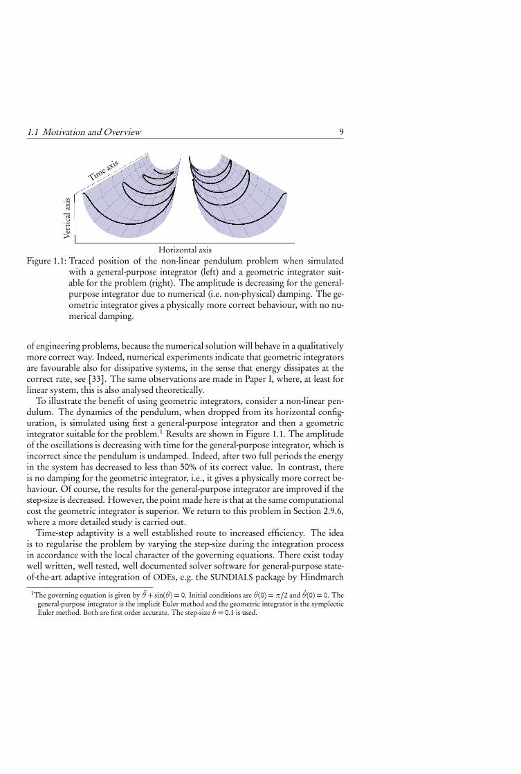
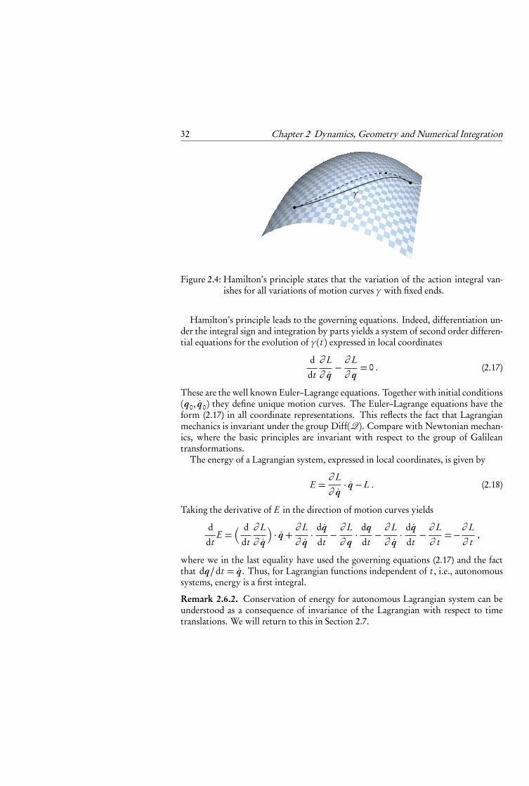
Figure 1.1: Traced position of the non-linear pendulum problem when simulatedwith a general-purpose integrator (left) and a geometric integrator suit-able for the problem (right). The amplitude is decreasing for the general-purpose integrator due to numerical (i.e. non-physical) damping. The ge-ometric integrator gives a physically more correct behaviour, with no nu-merical damping.
of engineering problems, because the numerical solution will behave in a qualitativelymore correct way. Indeed, numerical experiments indicate that geometric integratorsare favourable also for dissipative systems, in the sense that energy dissipates at thecorrect rate, see [33]. The same observations are made in Paper I, where, at least forlinear system, this is also analysed theoretically.
To illustrate the benefit of using geometric integrators, consider a non-linear pen-dulum. The dynamics of the pendulum, when dropped from its horizontal config-uration, is simulated using first a general-purpose integrator and then a geometricintegrator suitable for the problem.1 Results are shown in Figure 1.1. The amplitudeof the oscillations is decreasing with time for the general-purpose integrator, which isincorrect since the pendulum is undamped. Indeed, after two full periods the energyin the system has decreased to less than 50% of its correct value. In contrast, thereis no damping for the geometric integrator, i.e., it gives a physically more correct be-haviour. Of course, the results for the general-purpose integrator are improved if thestep-size is decreased. However, the point made here is that at the same computationalcost the geometric integrator is superior. We return to this problem in Section 2.9.6,where a more detailed study is carried out.
Time-step adaptivity is a well established route to increased efficiency. The ideais to regularise the problem by varying the step-size during the integration processin accordance with the local character of the governing equations. There exist todaywell written, well tested, well documented solver software for general-purpose state-of-the-art adaptive integration of ODEs, e.g. the SUNDIALS package by Hindmarch
1The governing equation is given by θ+ sin(θ) = 0. Initial conditions are θ(0) = π/2 and θ(0) = 0. Thegeneral-purpose integrator is the implicit Euler method and the geometric integrator is the symplecticEuler method. Both are first order accurate. The step-size h = 0.1 is used.
10 Chapter 1 Introduction
et. al. [27].During the early development and analysis of geometric integration methods, it
was noticed by Gladman et. al. [18] and by Calvo and Sanz-Serna [10] that if stan-dard time-step adaptivity is added to a geometric integrator its “physically correct”behaviour is lost. The reason for this is that the discrete dynamical system constitutedby the integrator is altered in such a way that the favourable phase space properties,making it a geometric integrator, are destroyed.
It was soon realised that a feasible path towards adaptive geometric integration is tointroduce a time transformation of the original problem, and then to utilise geometricintegration of the transformed system, see [52, 49, 21, 29, 9, 44, 12, 28, 42, 8, 26].This approach, however, is not without difficulties. Indeed, there are still many openproblems, in particular on how to construct adaptive geometric integrators that arefully explicit. Much of the work in this thesis is concerned with the problem ofcombining geometric integration with adaptivity.
We continue with a brief description of the BEAST software, and then the organi-sation of the thesis and an overview of the contributions.
1.1.1 The BEAST Software Environment
The software environment BEAST, for dynamic multibody simulations and post pro-cessing, is developed and maintained at SKF. It is used as a tool for better understand-ing of the dynamic behaviour of rolling bearings and other machine elements. Con-trary to other software packages, such as ADAMS [47] and SIMPACK [19], BEAST isspecifically designed for the accurate modelling of contacts between components. In-deed, the mechanical models used are highly complex, and are the result of extensiveinternal, as well as external, research on tribology [48].
The package essentially contains three parts: a preprocessing tool, a tool for thecomputation, and a postprocessing tool for the evaluation of the results. The com-putations are carried out on a high performance computer cluster located at SKF. Atypical simulation takes between 5–200 hours to carry out (depending on the numberof cluster nodes and complexity of the model).
1.1.2 Composition of Thesis and Contributions
This thesis is compiled out of an integrating part, containing five chapters, and inaddition five separate papers. The idea is that the first part should give a concisepresentation of the various theories and techniques used in the research, and to makereferences to the specific papers that contain the actual contributions.
Paper I deals with structure preserving integration of non-autonomous classicalengineering problems, such as rotor dynamics. It is shown, both numerically and bybackward error analysis, that geometric (structure preserving) integration algorithms

1.2 Preliminaries 11
are indeed superior to conventional Runge–Kutta methods. In addition to the spe-cific contributions, this paper can also be seen as a motivation for using geometricintegration schemes for engineering problems.
Paper II contains results on how to make the class of variational integrators adap-tive for general scaling objectives. Further, a scaling objective suitable for multibodyproblems with impact force laws is derived. Numerical examples are given.
Paper III concerns the problem of constructing explicit symplectic adaptive in-tegrators. A new approach based on Hamiltonian splitting and Sundman transfor-mations is introduced. Backward error analysis is used to analyze long time energyconservation. Numerical examples validating the energy behavior are given.
Paper IV develops a time transformation technique for Nambu–Poisson systems.Its structural properties are examined. The application in mind is adaptive numericalintegration by splitting of Nambu–Poisson Hamiltonians. As an example, a novelintegration method for the rigid body problem is presented and analysed.
Paper V sets forth an integration method particularly efficient for multibody prob-lems with contact between bodies. Stability analysis of the proposed method is car-ried out. Numerical examples are given for a simple test problem and for an industrialrolling bearing problem (using BEAST).
1.2 Preliminaries
Some prerequisites in analytical mechanics and differential geometry are assumedthroughout the text. Familiarity with the material in Chapter 1–9 of Arnold’s bookon classical mechanics [5] is recommended, although parts of it is repeated in Chap-ter 2 of the thesis. Furthermore, a certain acquaintance with symplectic integratorsand their analysis is assumed.

12 Chapter 1 Introduction

Chapter 2
Dynamics, Geometry and Numerical Integration
Many modern mathematical theories arose from problems inmechanics and only later acquired that axiomatic-abstract formwhich makes them so hard to study.
(V.I. Arnold, [5, p. v])
Many of the greatest mathematicians – Euler, Gauss, Lagrange,Riemann, Poincaré, Hilbert, Birkhoff, Atiyah, Arnold, Smale –were well versed in mechanics and many of the greatestadvances in mathematics use ideas from mechanics in afundamental way. Why is it no longer taught as a basic subjectto mathematicians?
(J.E. Marsden, [37, p. iv])
Summary In this chapter we give a concise exposition of the theory of dynamicalsystems, phase space geometry and geometric numerical integration. In particular wereview some fundamental concepts of analytical mechanics that are needed in order tounderstand the construction and analysis of geometric methods for mechanical prob-lems. As a general framework for structure preservation, the notion of classifyingvarious types of dynamical systems according to corresponding sub-groups of diffeo-morphisms is introduced. This viewpoint is then stressed throughout the remainderof the text.
2.1 Linear Systems
A square matrix A ∈ �n×n determines a linear vector field on �n by associating toeach x ∈ �n the vector Ax ∈ �n . Thus, it determines a set of linear (autonomous)ordinary differential equations of the form
dx
dt=Ax . (2.1)
13

14 Chapter 2 Dynamics, Geometry and Numerical Integration
These are the governing equations for the corresponding linear system: they describethe evolution in time of the coordinate vector x = (x1, . . . , xn). The flow of the systemis given by the matrix exponential exp(tA) (see Arnold [6], Chapter 3 for details).That is, the solution curve γ : �→ �n with initial data x at t = 0 is given by γ (t ) =exp(tA)x . Recall the following properties of the matrix exponential:
1. exp(A)−1 = exp(−A),
2.d
dtexp(tA) =Aexp(tA),
3. exp(diag(d1, . . . , dn)) = diag(ed1 , . . . , edn ),
4. exp((s + t )A) = exp(sA)exp(tA).
The last property, called the group property, originates from the fact that exp(tA)x0is the solution to an autonomous differential equation with initial data x0. Thus, ad-vancing the solution from x0 with time step s + t is the same as first advancing fromx0 with time step s landing on x1, and then advancing from there with time step t .This reasoning is valid also for non-linear autonomous initial value problems, whichis the basis for generalising the matrix exponential to non-linear vector fields (see Sec-tion 2.3).
The problem of constructing a good numerical integration scheme for (2.1) meansto find a map Φh : �n → �n , depending on a step size parameter h, such that Φhapproximates exp(hA) : �n → �n well. In the classical numerical analysis sense “ap-proximates well” means that Φh (x)− exp(hA)x should be small, i.e., the local errorshould be small, and that the scheme is stable. In addition, one may also ask thatΦh shares structural properties with exp(hA). For example that the method is linear,i.e., that it is of the form Φh (x) = R(hA)x for some map R : �n×n → �n×n with theproperty R(0) = Id. Already this allows for some structural analysis of the numericalsolution. Indeed, it is well known that the matrix exponential, when seen as a mapexp :�n×n→�n×n , is invertible in a neighbourhood of the identity, i.e., that the ma-trix logorithm log :�n×n →�n×n is well defined in a neighbourhood of the identitymatrix. Thus, the numerical method may be written Φh (x) = exp(log(R(hA)))x (forsmall enough h). By defining Ah = log(R(hA))/h we see that Φh is the exact flow ofthe modified linear differential equation x = Ah x . That is, Φh (x) = exp(hAh )x .
This is the notion of backward error analysis: to find a modified differential equa-tion whose exact solution reproduces the numerical approximation. It allows forqualitative conclusions about the numerical scheme. For example, from our analysiswe can immediately draw the conclusion that structural properties which are true forflows of linear systems also are true for linear numerical methods. Since most nu-merical integration schemes are linear (e.g. Runge–Kutta methods), this is not a verystrong result. As a more delicate example, assume that the matrix A in (2.1) has purely

2.1 Linear Systems 15
imaginary eigenvalues. It is then known that the solution is oscillating with constantamplitudes. Thus, for a qualitatively correct behaviour of the numerical solution it isof importance that also the eigenvalues of Ah are purely imaginary. This is certainlynot the case in general. For example, not for the explicit and the implicit Euler meth-ods. In order to carry out the analysis in this case one has to find a relation betweenproperties of A and properties of exp(hA) and then relate this to properties of R(hA).The standard tool at hand, also applicable for non-linear systems, is the theory of Liegroups and Lie algebras which is reviewed in Section 2.4.
2.1.1 Exterior Algebra of a Vector Space
In this section we review some exterior algebra of vector spaces. These results arelater generalised to manifolds. For a reference, see Hörmander [30, Sect. 6.2, A1–A2]or Abraham et. al. [2, Ch. 6]. Later on, the results from this section are helpful in thestudy of Poisson systems and Nambu mechanics.
Let V denote a real vector space of finite dimension n. Its dual space is denoted V∗.Recall that (V∗)∗ is identified with V. Further, the vector space of multilinear alternat-ing maps (V∗)k → � is denoted
∧kV. Thus,
∧kV∗ denotes multilinear alternating
maps Vk →�. Notice that∧1
V∗ = V∗ and∧0
V∗ ≡�. Also, recall that if θ ∈∧kV∗
and η ∈∧lV∗, then the exterior product between them is an element θ∧η ∈∧k+l
V∗.A basis ε1, . . . ,εn in V∗ induces a basis εi1
∧ · · · ∧ εikin∧k
V∗.
Proposition 2.1.1. Let W be a real vector space, and let S : (V∗)k →W be an alternatingmultilinear map. Then S has a unique representation on the form
S : (V∗)k � (ν1, . . . , νk ) �→ S(ν1 ∧ · · · ∧ νk )where S is a linear map
∧kV∗ →W.
Proof. See Hörmander [30].
Corollary 2.1.1. Every linear map T : V→W induces a linear map∧k T :
∧kV→∧k
W.
Proof. The map
Vk � (v1, . . . , vk ) �→ T (v1)∧ · · · ∧T (vk ) ∈k∧
W
is alternating and multilinear. Thus, by Proposition 2.1.1 it corresponds to a uniquemap
∧kV→∧k
W.
16 Chapter 2 Dynamics, Geometry and Numerical Integration
An immediate consequence of Proposition 2.1.1 is the following generalisation ofthe fact that (V∗)∗ is identified with V.
Corollary 2.1.2. The dual space (∧k
V∗)∗ is identified with∧k
V.
Proof. An elements w ∈ ∧kV is a multilinear alternating map (V∗)k → �. From
Proposition 2.1.1 with W = � it follows that w is identified with a unique map w :∧kV→�, i.e., w ∈ (∧k
V∗)∗.
From now on we will not separate w ∈∧kV from w ∈ (∧k
V∗)∗. Thus, elementsin∧k
V∗ act on elements in∧k
V and vice verse by dual pairing, just like elements inV∗ act on elements in V.
2.1.2 Non-homogenous and Non-autonomous Systems
A linear system is called non-homogenous if it is of the form
dx
dt=Ax + b (2.2)
for some element b ∈�n\{0}. Further, a system is called non-autonomous (and non-homogenous) if it is of the form
dx
dt=A(t )x + b(t ) (2.3)
where A : �→ �n×n and b : �→ �n are (possibly) time-dependent coefficients ofthe system.
From a non-autonomous and non-homogenous system of the form (2.3) it is alwayspossible to get an autonomous homogenous system by
d
dt
⎛⎜⎝xtξ
⎞⎟⎠=⎛⎜⎝A(t ) 0 b(t )
0 0 10 0 0
⎞⎟⎠⎛⎜⎝x
tξ
⎞⎟⎠ (2.4)
where ξ is an additional dummy variable with initial value 1.However, from a structural point of view one has to be careful when doing such
transformations. For example, notice that (2.4) is not a linear system. In Paper I amore detailed analysis of non-autonomous systems is carried out in terms of classi-fying suitable Lie sub-algebras. A typical application for problems of this form isclassical rotor dynamics.
2.1 Linear Systems 17
2.1.3 Study: Linear Rotor Dynamics
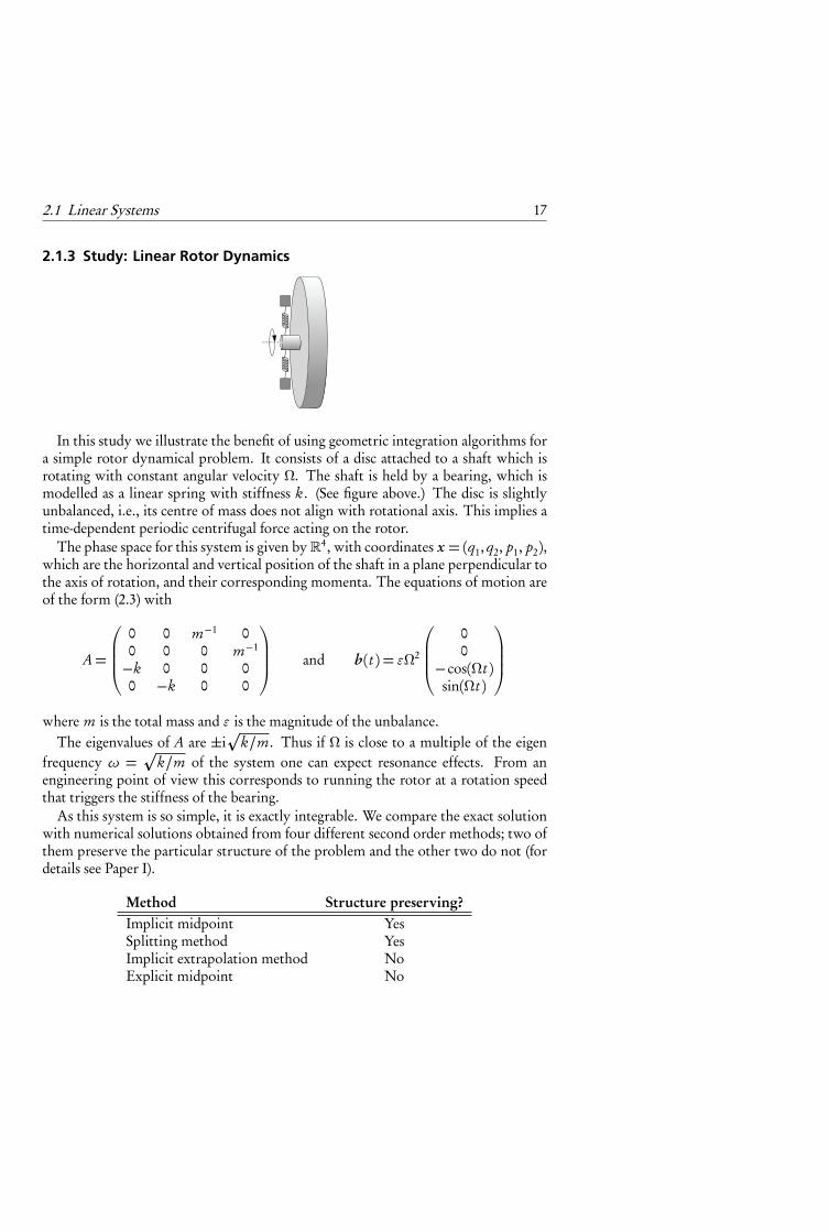
In this study we illustrate the benefit of using geometric integration algorithms fora simple rotor dynamical problem. It consists of a disc attached to a shaft which isrotating with constant angular velocity Ω. The shaft is held by a bearing, which ismodelled as a linear spring with stiffness k. (See figure above.) The disc is slightlyunbalanced, i.e., its centre of mass does not align with rotational axis. This implies atime-dependent periodic centrifugal force acting on the rotor.
The phase space for this system is given by�4, with coordinates x = (q1, q2, p1, p2),which are the horizontal and vertical position of the shaft in a plane perpendicular tothe axis of rotation, and their corresponding momenta. The equations of motion areof the form (2.3) with
A=
⎛⎜⎜⎜⎝0 0 m−1 00 0 0 m−1
−k 0 0 00 −k 0 0
⎞⎟⎟⎟⎠ and b(t ) = εΩ2
⎛⎜⎜⎜⎝00
−cos(Ωt )sin(Ωt )
⎞⎟⎟⎟⎠where m is the total mass and ε is the magnitude of the unbalance.
The eigenvalues of A are ±i
k/m. Thus if Ω is close to a multiple of the eigenfrequency ω =
k/m of the system one can expect resonance effects. From an
engineering point of view this corresponds to running the rotor at a rotation speedthat triggers the stiffness of the bearing.
As this system is so simple, it is exactly integrable. We compare the exact solutionwith numerical solutions obtained from four different second order methods; two ofthem preserve the particular structure of the problem and the other two do not (fordetails see Paper I).
Method Structure preserving?Implicit midpoint YesSplitting method YesImplicit extrapolation method NoExplicit midpoint No
18 Chapter 2 Dynamics, Geometry and Numerical Integration
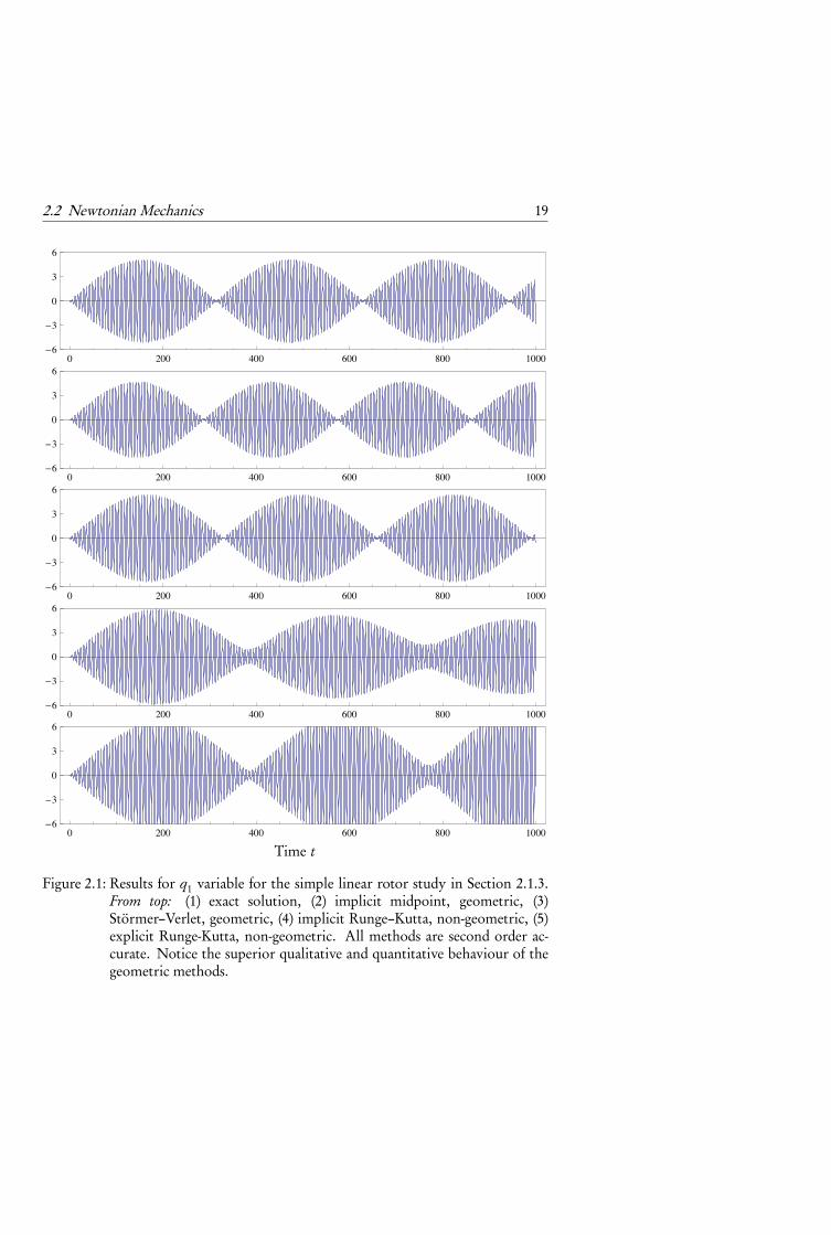
Results are shown in Figure 2.1. Notice that the geometric methods are superioras they give the qualitatively correct behaviour. This behaviour is explained theoreti-cally in Paper I using backward error analysis.
2.2 Newtonian Mechanics
Newtonian mechanics deals with the dynamics of interacting particles. Each parti-cle “lives” in a four dimensional affine space A4 equiped with a Galilean space–timestructure. Points e ∈ A4 are called events. Since A4 is an affine space, the differencebetween events is well defined, and the set of all differences between elements in A4
constitutes the linear space �4.The Galilean space–time structure consists of the following:
1. A linear map t : �4→ � called time. Two events e1 and e2 are simultaneous ift(e1− e2) = 0.
2. The linear space of simultaneous events, i.e., ker(t) ≡ �3, is equiped with anEuclidean structure ⟨·|·⟩. Thus, it is possible to measure the distance betweentwo events in ker(t). Notice, however, that one cannot measure the distancebetween non-simultaneous events, unless a coordinate system has been intro-duced in A4 as a reference.
Coordinates in A4 given by (r , t ) = (r 1, r 2, r 3, t ) are called Galilean coordinatesif r are orthogonal coordinates in ker(t) and t − t(r , t ) = const. A curve in A4 thatappears as the graph of some motion t �→ r (t ) is called a world line. Thus, the motionof a system of n particles consists of n world lines.
The most fundamental principle in Newtonian mechanics is Newton’s equations.These equations describe the motion t �→ (r 1(t ), . . . , r n(t )) of n interacting particles.They constitute a system of second order differential equations on the form
mi
d2r i
dt 2= F i +F ext
i , i = 1, . . . , n . (2.5)
Here, mi > 0 denotes the mass of particle i , F i the force exerted on particle i bythe other particles, and F ext
i the external forces. By introducing coordinates x =(r 1, . . . , r n), on the configuration space, i.e., the space of all possible positions theparticles can have, the governing equations can be written in the more compact form
Md2x
dt 2= F +F ext , (2.6)
where M = diag(m1, . . . , mn), F = (F 1, . . . ,F n) and F = (F ext1 , . . . ,F ext
n ).
2.2 Newtonian Mechanics 19
0 200 400 600 800 1000�6
�3
0
3
6
0 200 400 600 800 1000�6
�3
0
3
6
0 200 400 600 800 1000�6
�3
0
3
6
0 200 400 600 800 1000�6
�3
0
3
6
0 200 400 600 800 1000�6
�3
0
3
6
Time t
Figure 2.1: Results for q1 variable for the simple linear rotor study in Section 2.1.3.From top: (1) exact solution, (2) implicit midpoint, geometric, (3)Störmer–Verlet, geometric, (4) implicit Runge–Kutta, non-geometric, (5)explicit Runge-Kutta, non-geometric. All methods are second order ac-curate. Notice the superior qualitative and quantitative behaviour of thegeometric methods.
20 Chapter 2 Dynamics, Geometry and Numerical Integration
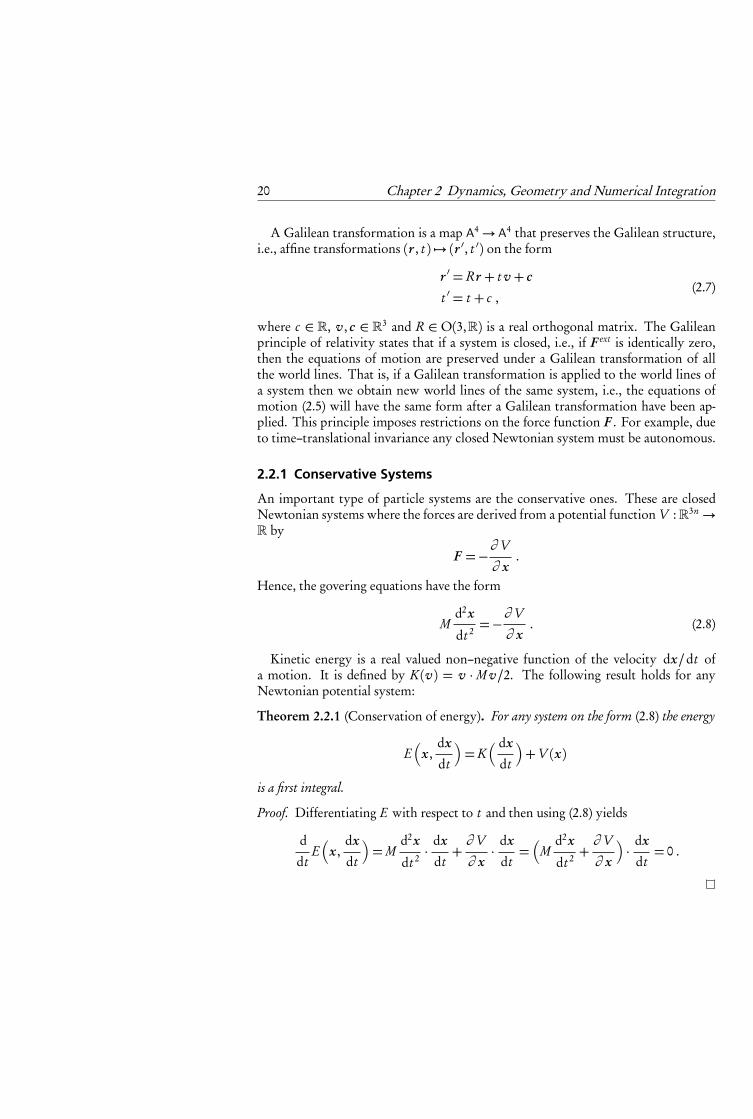
A Galilean transformation is a map A4→ A4 that preserves the Galilean structure,i.e., affine transformations (r , t ) �→ (r ′, t ′) on the form
r ′ = Rr + t v + c
t ′ = t + c ,(2.7)
where c ∈ �, v, c ∈ �3 and R ∈ O(3,�) is a real orthogonal matrix. The Galileanprinciple of relativity states that if a system is closed, i.e., if F ext is identically zero,then the equations of motion are preserved under a Galilean transformation of allthe world lines. That is, if a Galilean transformation is applied to the world lines ofa system then we obtain new world lines of the same system, i.e., the equations ofmotion (2.5) will have the same form after a Galilean transformation have been ap-plied. This principle imposes restrictions on the force function F . For example, dueto time–translational invariance any closed Newtonian system must be autonomous.
2.2.1 Conservative Systems
An important type of particle systems are the conservative ones. These are closedNewtonian systems where the forces are derived from a potential function V :�3n→� by
F =−∂ V
∂ x.
Hence, the govering equations have the form
Md2x
dt 2=−∂ V
∂ x. (2.8)
Kinetic energy is a real valued non–negative function of the velocity dx/dt ofa motion. It is defined by K(v) = v · M v/2. The following result holds for anyNewtonian potential system:
Theorem 2.2.1 (Conservation of energy). For any system on the form (2.8) the energy
E�
x ,dx
dt
�=K
� dx
dt
�+V (x)
is a first integral.
Proof. Differentiating E with respect to t and then using (2.8) yields
d
dtE�
x ,dx
dt
�=M
d2x
dt 2· dx
dt+∂ V
∂ x· dx
dt=�
Md2x
dt 2+∂ V
∂ x
�· dx
dt= 0 .
2.3 Manifolds 21
U
U′
χ
χ ′
χ (U)
χ ′(U′)
χ ′ ◦χ−1
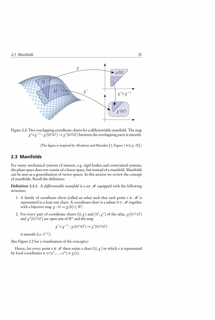
Figure 2.2: Two overlapping coordinate charts for a differentiable manifold. The mapχ ′ ◦χ−1 : χ (U∩U′)→ χ ′(U∩U′) between the overlapping parts is smooth.
(The figure is inspired by Abraham and Marsden [1, Figure 1.4-2; p. 32].)
2.3 Manifolds
For many mechanical systems of interest, e.g. rigid bodies and constrained systems,the phase space does not consist of a linear space, but instead of a manifold. Manifoldscan be seen as a generalisation of vector spaces. In this section we review the conceptof manifolds. Recall the definition:
Definition 2.3.1. A differentiable manifold is a set M equipped with the followingstructure:
1. A family of coordinate charts (called an atlas) such that each point x ∈ M isrepresented in a least one chart. A coordinate chart is a subset U⊂M togetherwith a bijective map χ : U→ χ (U)⊂�n .
2. For every pair of coordinate charts (U,χ ) and (U′,χ ′) of the atlas, χ (U ∩ U′)and χ ′(U∩U′) are open sets of �n and the map
χ ′ ◦χ−1 : χ (U∩U′)→ χ ′(U∩U′)
is smooth (i.e. C∞).
(See Figure 2.2 for a visualisation of the concepts.)
Hence, for every point x ∈M there exists a chart (U,χ ) in which x is representedby local coordinates x = (x1, . . . , xn) = χ (x).
22 Chapter 2 Dynamics, Geometry and Numerical Integration
Remark 2.3.1. Throughout the rest of the text we sometimes write x ∈M to denotea point in M represented by local coordinates. This abuse of notation is generallyaccepted in the literature.
It follows from the definition that transformation between any two different coor-dinate representations is smooth. This, in turn, implies that the dimension n of M iswell defined. Furthermore, if an assertion about differentiability is made in one coor-dinate representation, it automatically holds also in other coordinate representations.Hence, ordinary calculus as developed in �n may be used also on manifolds.
Remark 2.3.2. Two atlases A and A′ of M are called equivalent if A ∪A′ is againan atlas of M . The equivalence class of equivalent atlases specifies a differentiablestructure on M . A differentiable structure may or may not be unique. For example,all differentiable manifolds of dimension 3 or less have unique differentiable struc-tures, whereas S7 admits 28 differentiable structures, as pointed out by J. Milnor in1956. Before that it was thought that a topological space admits only one differen-tiable structure. Throughout the rest of the text, we assume that every manifold isequipped with its maximal atlas, i.e., the atlas containing all its equivalent atlases.
Differentiability of maps between manifolds is defined as follows:
Definition 2.3.2. Let M and R be two differentiable manifolds of dimension nand m respectively. A map ϕ : M →R is called differentiable at x ∈M if
ψ ◦ϕ ◦χ−1 :�n→�m
is differentiable at χ (x) for some coordinate charts (U,χ ) containing x and (V,ψ)containing ϕ(x).
Notice that the definition of differentiability is independent on the coordinatecharts used. Indeed, differentiability is preserved in all coordinate representations,since transformation between coordinates is smooth. The definition of C r maps fol-lows as in ordinary calculus.
Remark 2.3.3. If ϕ : M → R is smooth and bijective with a smooth inverse, ϕ iscalled a diffeomorphism. M and R are then diffeomorphic, meaning that they areessentially the same space (at least when looked upon as manifolds). The set of dif-feomorphisms M →M is a group denoted by Diff(M ). Principles in Lagrangianmechanics (see Section 2.6) are invariant with respect to coordinate transformations,and thus, also with respect to this group of transformations. Compare with Newto-nian mechanics, where principles are invariant with respect to the Galilean group oftransformations.
To specify the equations of motion of a dynamical system it is necessary to considerderivatives of curves in manifolds. The derivative of a curve in a vector space is again

2.3 Manifolds 23
a curve in the vector space. For curves in manifolds this is not the case. Recollectthe following concepts, which are needed in order to speak of derivatives of mapsbetween manifolds:
Definition 2.3.3. A tangent vector v at a point x ∈ M is an equivalence class ofdifferentiable curves �→M , where the equivalence relation for two curves γ1 andγ2 is given by
γ1(0) = γ2(0) = x andd(χ ◦ γ1)(t )
dt
t=0=
d(χ ◦ γ2)(t )
dt
t=0
for some coordinate chart (U,χ ) containing x.
Definition 2.3.4. The tangent space of M at x is the set of all tangent vectors at x,and is denoted TxM . It is a linear space of dimension n, where αv1+βv2 is definedby the equivalence class of curves γ3 that fulfils
γ3(0) = x andd(χ ◦ γ3)(t )
dt
t=0=�α
d(χ ◦ γ1)(t )
dt+β
d(χ ◦ γ2)(t )
dt
� t=0
,
where γ1 and γ2 are representatives for v1 and v2 respectively.
Definition 2.3.5. The tangent bundle of M is the union of all the tangent spaces, i.e.,the set
TM =⋃
x∈MTxM .
An element in TM which is in TxM is denoted vx. The map π : TM →M givenby π : vx �→ x is called the natural projection. A C 1 map X : M → TM such thatπ ◦X = Id is called a vector field. Every vector field is intrinsically associated with adifferential equation dx/dt =X (x).
Definition 2.3.6. The cotangent space of M at x is the dual space of TxM , i.e., thespace of linear forms on TxM . It is denoted T ∗
xM .
Definition 2.3.7. The cotangent bundle of M is the union of all the cotangent spaces:
T ∗M =⋃
x∈MT ∗
xM .
The natural projection π : T ∗M →M is defined accordingly.
Remark 2.3.4. The tangent bundle TM and the cotangent bundle T ∗M both havethe structure of differentiable manifolds with dimension 2n. Below we discuss howcoordinate charts in M naturally introduce coordinate charts in TM and T ∗M .
24 Chapter 2 Dynamics, Geometry and Numerical Integration
TxM
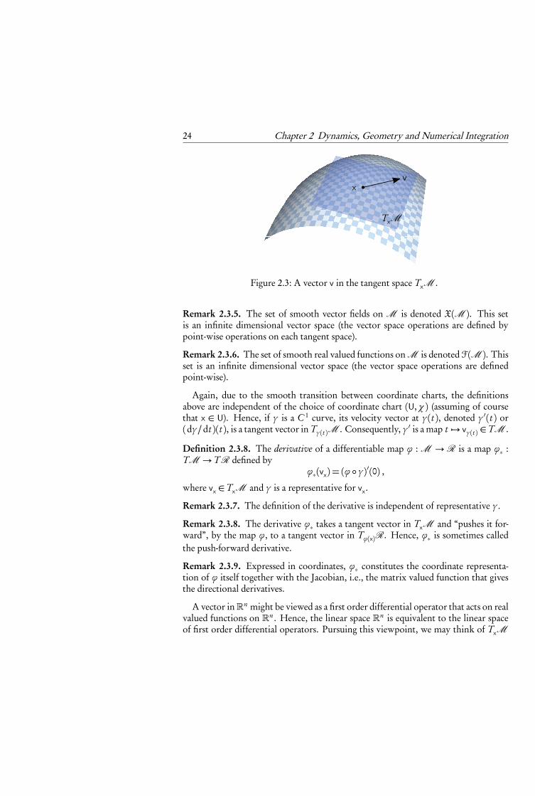
xv
Figure 2.3: A vector v in the tangent space TxM .
Remark 2.3.5. The set of smooth vector fields on M is denoted X(M ). This setis an infinite dimensional vector space (the vector space operations are defined bypoint-wise operations on each tangent space).
Remark 2.3.6. The set of smooth real valued functions on M is denoted F(M ). Thisset is an infinite dimensional vector space (the vector space operations are definedpoint-wise).
Again, due to the smooth transition between coordinate charts, the definitionsabove are independent of the choice of coordinate chart (U,χ ) (assuming of coursethat x ∈ U). Hence, if γ is a C 1 curve, its velocity vector at γ (t ), denoted γ ′(t ) or(dγ/dt )(t ), is a tangent vector in Tγ (t )M . Consequently, γ ′ is a map t �→ vγ (t ) ∈ TM .
Definition 2.3.8. The derivative of a differentiable map ϕ : M → R is a map ϕ∗ :TM → T R defined by
ϕ∗(vx) = (ϕ ◦ γ )′(0) ,where vx ∈ TxM and γ is a representative for vx.
Remark 2.3.7. The definition of the derivative is independent of representative γ .
Remark 2.3.8. The derivative ϕ∗ takes a tangent vector in TxM and “pushes it for-ward”, by the map ϕ, to a tangent vector in Tϕ(x)R. Hence, ϕ∗ is sometimes calledthe push-forward derivative.
Remark 2.3.9. Expressed in coordinates, ϕ∗ constitutes the coordinate representa-tion of ϕ itself together with the Jacobian, i.e., the matrix valued function that givesthe directional derivatives.
A vector in�n might be viewed as a first order differential operator that acts on realvalued functions on �n . Hence, the linear space �n is equivalent to the linear spaceof first order differential operators. Pursuing this viewpoint, we may think of TxM
2.3 Manifolds 25
as the linear space of first order differential operators acting on smooth real valuedfunctions on M by taking the derivative of them at x in some direction. Indeed, if γis a representative for vx ∈ TxM and f ∈ F(M ), then the differential operator
vx[ f ] =d
dt( f ◦ γ )(t )
t=0
is well defined. Expressed in local coordinates we get
vx[ f ] =d
dt( f ◦χ−1 ◦χ ◦ γ )(t )
t=0=∂ f (x)
∂ x· d(χ ◦ γ )(t )
dt
t=0
(2.9)
Remark 2.3.10. Notice the abuse of notation: ∂ f (x)/∂ x really means ∂ ( f ◦χ−1)(x)/∂ x .
Remark 2.3.11. The differential operator intrinsically associated with a vector field Xon M (by taking derivatives in the direction of the vector field) is called the Lie deriva-tive and is denoted LX . Thus, L acts on f ∈ F(M ) by (LX f )(x) = X (x)[ f ]. The Liederivative can be extended to act on any geometric object on M (e.g. vector fields,tensor fields, differential forms) by taking the derivative of them in the direction of X ,see [1, Sect. 2.2]
A natural basis in TxM is given by ∂ /∂ x1, . . . ,∂ /∂ xn . Indeed, from (2.9) we seethat every element v ∈ TxM is uniquely represented in this basis as
vx =n∑
i=1
x i ∂
∂ xi= x · ∂
∂ x,
where x = d(χ ◦γ )(t )/dt |t=0. Hence, from coordinates x in M we have constructedcoordinates x in TxM . Furthermore, the pair (x , x) constitutes local coordinatesfor TM , called natural coordinates. The significance of natural coordinates lies inthe fact that if the derivative γ ′(t ) of a curve is represented in natural coordinates as(x(t ), x(t )), then it holds that dx(t )/dt = x(t ).
Remark 2.3.12. A basis in a vector space induces a dual basis in the dual vector space.Hence, the basis ∂ /∂ x1, . . . ,∂ /∂ xn in TxM induces a dual basis e1, . . . , en in T ∗
xM .
Recall that ⟨e i ,∂ /∂ x j ⟩ = δi j . From this we see that e i = dxi (projection of vectorsonto the xi axis). Hence, every element p ∈ T ∗
xM can be written as
∑i pi dxi =
p dx , and (x , p) constitutes a coordinate chart in T ∗M . These are called canonicalcoordinates.
2.3.1 Exterior Algebra of a Manifold
In this section we extend the concept of exterior algebra for vector spaces, reviewedin Section 2.1.1, to manifolds.
26 Chapter 2 Dynamics, Geometry and Numerical Integration
Let again M denote a smooth manifold. The linear spaces∧k T ∗x M are the fibers
of a vector bundle∧k T ∗M . The space of differential k–forms on M is the space
of sections C∞(M ,∧k T ∗M ). It is denoted Λk (M ). Likewise, the space of con-
travariant totally antisymmetric smooth k–tensor fields, i.e., the space of sectionsC∞(M ,
∧k TM ), is denoted Ωk (M ). Notice that Λ0(M ) = Ω0(M ) = F(M ), i.e.,the space of smooth functions on M . Further, Ω1 = X(M ), which is the space ofsmooth vector fields on M .
An easily discerned viewpoint for the extension of exterior algebra to manifolds,is to think of the scalar field � as replaced by the algebra F(M ) of smooth func-tion on M and the vector space V replace by X(M ). With this viewpoint, Ωk (M )and Λk (M ) are dual to each other, since each pair of corresponding fibers are dual.Thus, all the algebraic operations above for
∧kV∗ and
∧kV carrie over to Ωk (M )
and Λk (M ). Notice that the pairing between an element in Ωk (M ) and another inΛk (M ) gives an element in F(M ).
2.4 Lie Groups and Lie Algebras
The theory of Lie groups and Lie algebras is essential in the theory of dynamicalsystems and geometry of phase space. In our application they appear in several ways:
• For many mechanical systems the configuration space is a Lie group. The mosttypical example is the rigid body, which evolves on the Lie group of rotations(see Section 2.8).
• Symmetries of mechanical systems, leading to various conservation laws, aredescribed in terms of Lie groups (see Section 2.7).
• In geometric integration, infinite dimensional Lie groups appear as sub-groupsof the group of diffeomorphisms on a phase space manifold. This is an impor-tant view-point, which is the key to geometric integration and backward erroranalysis. (see Section 2.5).
Recall that a Lie group is a differentiable manifold G equipped with a group struc-ture, such that the group multiplication G × G � (g , h) �→ g h ∈ G is smooth. Let edenote the identity element.
A Lie group acts on itself by left and right translation:
Lg : G � h �→ g h ∈ G ,
Rg : G � h �→ h g ∈ G .(2.10)
These maps are, for each g , diffeomorphisms on G . Indeed, the maps
L−1g = Lg−1 and R−1
g = Rg−1
2.4 Lie Groups and Lie Algebras 27
are smooth, since the group multiplication is smooth. The corresponding push-forward maps Lg∗ and Rg∗ are diffeomorphisms on T G such that
ThG � ξh �→ Lg∗(ξh ) ∈ Tg hG ,
and correspondingly for the right translation.Each vector ξ ∈ TeG defines a vector field Xξ on G by
Xξ (g ) = Lg∗(ξ ) . (2.11)
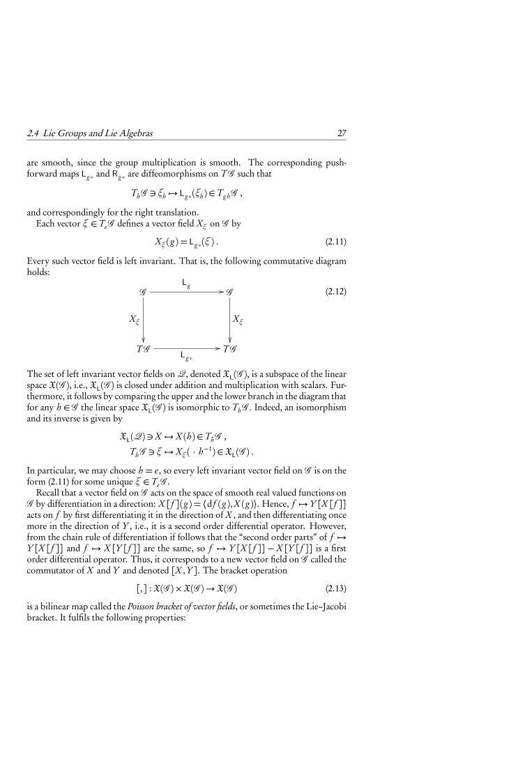
Every such vector field is left invariant. That is, the following commutative diagramholds:
GLg ��
Xξ
��
G
Xξ
��T G
Lg∗�� T G
(2.12)
The set of left invariant vector fields on Q, denoted XL(G ), is a subspace of the linearspace X(G ), i.e., XL(G ) is closed under addition and multiplication with scalars. Fur-thermore, it follows by comparing the upper and the lower branch in the diagram thatfor any h ∈ G the linear space XL(G ) is isomorphic to ThG . Indeed, an isomorphismand its inverse is given by
XL(Q) �X �→X (h) ∈ ThG ,
ThG � ξ �→Xξ ( · h−1) ∈XL(G ) .
In particular, we may choose h = e , so every left invariant vector field on G is on theform (2.11) for some unique ξ ∈ TeG .
Recall that a vector field on G acts on the space of smooth real valued functions onG by differentiation in a direction: X [ f ](g ) = ⟨d f (g ),X (g )⟩. Hence, f �→ Y [X [ f ]]acts on f by first differentiating it in the direction of X , and then differentiating oncemore in the direction of Y , i.e., it is a second order differential operator. However,from the chain rule of differentiation if follows that the “second order parts” of f �→Y [X [ f ]] and f �→ X [Y [ f ]] are the same, so f �→ Y [X [ f ]]−X [Y [ f ]] is a firstorder differential operator. Thus, it corresponds to a new vector field on G called thecommutator of X and Y and denoted [X ,Y ]. The bracket operation
[,] : X(G )×X(G )→X(G ) (2.13)
is a bilinear map called the Poisson bracket of vector fields, or sometimes the Lie–Jacobibracket. It fulfils the following properties:
28 Chapter 2 Dynamics, Geometry and Numerical Integration
1. skew symmetry, i.e., [X ,Y ] =−[Y,X ] ;
2. the Jacobi identity, i.e., [[X ,Y ],Z]+ [[Y,Z],X ]+ [[Z ,X ],Y ] = 0 .
A vector space equipped with a bilinear map that fulfils 1–2 above is called a Liealgebra. Thus, the Poisson bracket of vector fields (2.13) makes X(G ) into an infinitedimensional Lie algebra.
Remark 2.4.1. The definition of X(G ) as a Lie algebra is independent of the factthat G is a Lie group. Indeed, for any manifold M , the commutator makes X(M )into a Lie algebra.
Notice that if X ,Y ∈XL(G ) then
Lg∗�[X ,Y ](e)
�= [X ,Y ](g ) ,
so [X ,Y ] is left invariant, i.e., it belongs to XL(G ). This means that XL(G ) is closedunder the commutator (2.13), so it is a Lie subalgebra of X(G ). Furthermore, sinceXL(G ) is isomorphic to TeG the commutator also induces a Lie algebra structure inTeG . Indeed, for ξ ,η ∈ TeG the bracket operation [ξ ,η], now called the Lie bracket,is defined by
[Xξ ,Xη] =X[η,ξ ] . (2.14)
Definition 2.4.1. Let G be a Lie group. The vector space TeG equipped with the Liealgebra constructed above is called the Lie algebra of G and is denoted g.
Remark 2.4.2. The concepts developed above are based on left invariant vector fields:the Lie bracket defined by (2.14) is said to be defined by left extension. It is, of course,also possible to use the right invariant vector fields, and define a Lie bracket [,]R byright extension. The two algebras are then related by [,] =−[,]R.
If s , t ∈ � then for any ξ ∈ g we have that [sξ , tξ ] = s t[ξ ,ξ ] = 0, where thelast equality is due to skew symmetry of the Lie bracket. From this it follows thatthe subspace ξ� ⊂ g is actually a 1–dimensional Lie sub-algebra. It is, in fact, theLie algebra of the Lie sub-group that is generated by the solution curve through e ofthe left invariant vector field Xξ . Indeed, if γξ is a solution curve of Xξ such thatγξ (0) = e , then γξ (s + t ) = γξ (s )γξ (t ). γξ (t ) is called the one parameter subgroupof G generated by ξ .
Definition 2.4.2. The exponential map exp : g→ G is defined by exp(ξ ) = γξ (1).
Since Lg∗ is a linear map, it follows from (2.11) that sXξ = Xsξ , which impliesγξ (t ) = γtξ (1) = exp(tξ ).
2.5 Geometric Integration and Backward Error Analysis 29
Remark 2.4.3. The group of diffeomorphisms Diff(M ) is an infinite dimensional Liegroup. Its Lie algebra is given by X(M ), with the commutator (2.13) as Lie bracket.Pursuing this viewpoint, it follows that if X ∈ X(M ) then the flow of X is given bythe exponential map, i.e., ϕ t
X = exp(tX ).
Remark 2.4.4. The concept of infinite dimensional Lie groups is far more complexthan the finite dimensional case, due to the fact that the group operation needs to besmooth. Many assertions made for finite dimensional Lie groups and correspondingLie algebras are not true in general for infinite dimensional Lie groups. For example,the exponential maps needs not be locally invertible. Throughout the remainderof the text we will formally use infinite dimensional Lie groups in order to classifydifferent classes of maps and corresponding vector fields. We refer to McLachlan andQuispel [40] and Schmid [46] for further issues concerning infinite dimensional Liegroups.
2.5 Geometric Integration and Backward Error Analysis
In this section we review the basic scheme of geometric integration and backwarderror analysis. Our material is heavily inspired by Reich [45] and by McLachlan andQuispel [40]. See also the references [15, 20, 7, 22] for background.
Throughout this section M is the phase space manifold. We begin with a rigorousdefinition of what we mean by “an integrator.”
Definition 2.5.1 (One step integrator). A one step integrator is a continuous map
Φ :�×M � (h, x0) �→ x1 ∈M
such that Φ(0, ·) = Id. The first argument h is called the step size parameter. Thenumerical solution trajectory corresponding to Φ is the sequence x0, x1, . . . definedrecursively by x k+1 =Φ(h, x k ).
Remark 2.5.1. We sometimes write Φh = Φ(h, ·). The parameter h in Φh corre-sponds to t in the exact flow ϕ t
X . One important difference, however, is that Φh isnot (in general) a one parameter group, i.e., Φh ◦Φs �=Φh+s . If that had been the case,decreasing the step size parameter would not affect the accuracy of the integration.
Definition 2.5.2 (Order of consistency). The integrator Φh is said to be consistent oforder r relative to a dynamical system with flow ϕ t
X for some vector field X on M if
Φh (x)−ϕhX (x) =O(h r+1) .
for each x ∈M .
30 Chapter 2 Dynamics, Geometry and Numerical Integration
Now to geometry in phase space. A geometric integrator is, somewhat vaguely,a one step integrator that shares some qualitative property with its correspondingexact flow. A standard approach for classifying geometric integrators is obtainedthrough the framework of Lie groups and Lie algebras. Indeed, recall from Section 2.4that Diff(M ) is an infinite dimensional Lie group corresponding to the infinite di-mensional Lie algebra X(M ). Thus, a natural way to classify integrators is to considersub-groups of Diff(M ).
Let XS (M ) be a sub-algebra of X(M ), and DiffS (M ) its corresponding sub-groupof Diff(M ). Now, given a vector field X ∈ XS (M ) its flow t �→ ϕ t
X (x) is a one-parameter sub-group of DiffS (M ). In particular, ϕ t
X ∈ DiffS (M ) for each t .
Definition 2.5.3. An integrator Φh for X ∈XS (M ) is called geometric (with respectto DiffS (M )) if it holds that Φh ∈ DiffS (M ) for each h small enough.
Remark 2.5.2. Choosing DiffS (M ) = Diff(M ) we see that in principle all inte-grators are geometric with respect to Diff(M ). From now on we only denote anintegrator geometric when it belongs to a proper sub-group of Diff(M ).
Remark 2.5.3. In Reich [45] the concept of a geometric integrator is somewhat moregeneral in that XS (M ) not necessarily needs to be a Lie sub-algebra. This allowsalso the treatment of reversible integrators within the same framework. (The setof reversible maps does not form a Lie sub-group.) To make the presentation moretransparent we consider here only Lie sub-algebras.
The basic principle of backward error analysis is to look for a modified vector fieldXh ∈ XS (M ) such that ϕh
Xh= Φh . Recall from Section 2.4 that ϕ t
X = exp(tX ).
Thus, the objective is to find Xh such that exp(hXh ) = Φh . A formal solution isgiven by Xh = exp−1(Φh )/h. Thus, backward error analysis really is the question ofwhether the exponential map is invertible (at least in a neighbourhood of the iden-tity, i.e., when h is small). If DiffS (M ) is a finite dimensional sub-group, then it is awell known result that the exponential map is invertible in a neighbourhood of theidentity. However, as mentioned above things are much more complex in the infi-nite dimensional case. In this case one typically have to truncate a power series ofexp−1(Φh )/h about h = 0. In conjunction with a result that each term in the powerseries also is an element in XS (M ), this analysis implies that assertions of Xh are validfor exponentially long times, even though the power series does not converge. (SeeReich [45] for details.)
By carrying out backward error analysis, i.e., assuring that Xh ∈ XS (M ) (at leastformally), one can often draw deep conclusions about Φh . For example, if M is asymplectic manifold (see Section 2.9 below) and DiffS (M ) is the group of symplecticmaps one can assert that Xh is a Hamiltonian vector field. Thus Φh will preservea modified Hamiltonian function H (at least locally), which is close to the originalHamiltonian function of X . That is, the Hamiltonian is nearly preserved.
2.6 Lagrangian Mechanics 31
2.5.1 Splitting Methods
A simple yet powerful way to derive geometric integrators is by the vector field split-ting approach. Let X ∈ XS (M ) and assume that X can be splitted into simpler partsX = X A+X B , where both X A,X B ∈ XS (M ). The trick is that X A and X B shouldbe explicitly integrable, i.e., that ϕ t
X A and ϕ tX B can be explicitly computed. If that is
the case, a geometric integrator for X is obtained by composing ϕ tX A and ϕ t
X B to get agood approximation of ϕ t
X . The most popular choice is the Strang–splitting obtained
by Φh = ϕh/2X A ◦ϕh
X B ◦ϕh/2X A . For an extensive treatment of splitting methods and further
references see McLachlan and Quispel [41].
2.6 Lagrangian Mechanics
In Newtonian mechanics, the configuration space is a linear space of dimension 3n,and the basic principle for motion is expressed by Newton’s differential equations.For many physical systems, e.g. for constrained systems, this setting is not sufficientand more general configuration spaces must be considered. A particularly importantexample in our context is the rigid body. Here, the configuration space consists ofthe set of 3D–rotations, which is not a linear space. We discuss the rigid body and itsgoverning equations further in Section 2.8.
2.6.1 Hamilton’s Principle and the Euler–Lagrange Equations
Recall that a Lagrangian mechanical system consists of a configuration space Q, anda Lagrangian function TM ×� � (vq, t ) �→ L(vq, t ) ∈ �. Hamilton’s principle statesthat motions of Lagrangian systems extremise the action integral. More precisely, acurve γ : (a, b )→Q is a motion if
A(γ ) =∫ b
aL�γ ′(t ), t
�dt (2.15)
is extremised, i.e., its differential at γ vanishes for variations with fixed endpoints:
⟨dA(γ ),δγ ⟩= 0 , ∀ δγ ∈ TγC(Q) (2.16)
where
C(Q) = {C 2 curves (a, b )→Q with fixed endpoints γ (a) and γ (b )} .Remark 2.6.1. The set C(Q) is an infinite dimensional differentiable manifold. Anelement δγ ∈ TγC(Q) is a curve (a, b )→ TQ such that π ◦δγ (t ) = γ (t ).
32 Chapter 2 Dynamics, Geometry and Numerical Integration
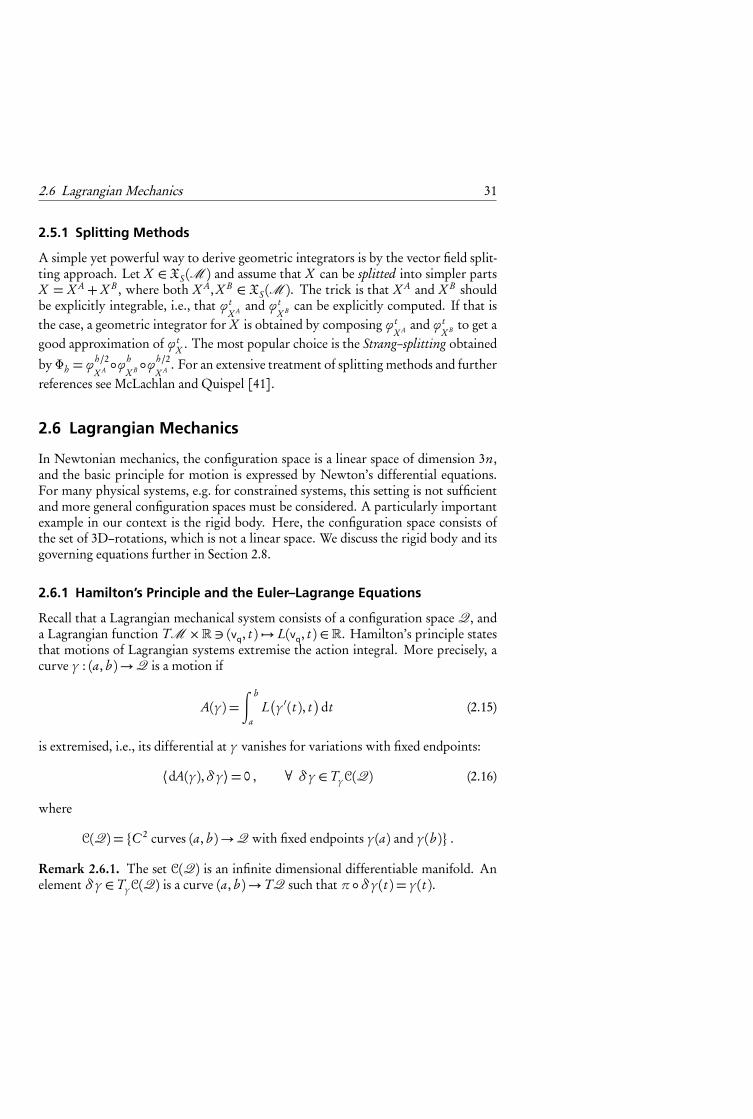
γ
Figure 2.4: Hamilton’s principle states that the variation of the action integral van-ishes for all variations of motion curves γ with fixed ends.
Hamilton’s principle leads to the governing equations. Indeed, differentiation un-der the integral sign and integration by parts yields a system of second order differen-tial equations for the evolution of γ (t ) expressed in local coordinates
d
dt
∂ L
∂ q− ∂ L
∂ q= 0 . (2.17)
These are the well known Euler–Lagrange equations. Together with initial conditions(q0, q0) they define unique motion curves. The Euler–Lagrange equations have theform (2.17) in all coordinate representations. This reflects the fact that Lagrangianmechanics is invariant under the group Diff(Q). Compare with Newtonian mechan-ics, where the basic principles are invariant with respect to the group of Galileantransformations.
The energy of a Lagrangian system, expressed in local coordinates, is given by
E =∂ L
∂ q· q − L . (2.18)
Taking the derivative of E in the direction of motion curves yields
d
dtE =
� d
dt
∂ L
∂ q
�· q + ∂ L
∂ q· dq
dt− ∂ L
∂ q· dq
dt− ∂ L
∂ q· dq
dt− ∂ L
∂ t=−∂ L
∂ t,
where we in the last equality have used the governing equations (2.17) and the factthat dq/dt = q. Thus, for Lagrangian functions independent of t , i.e., autonomoussystems, energy is a first integral.
Remark 2.6.2. Conservation of energy for autonomous Lagrangian system can beunderstood as a consequence of invariance of the Lagrangian with respect to timetranslations. We will return to this in Section 2.7.
2.6 Lagrangian Mechanics 33
Example 2.6.1 (Newtonian potential system). A Newtonian potential system is aspecial case of a Lagrangian system. Here, Q = �3n and the Lagrangian function isdefined by
L(x , x) = T (x)−V (x) =x ·M x
2−V (x) .
The Euler–Lagrange equations (2.17) for this system are exactly Newton’s differentialequations (2.8).
Remark 2.6.3. As can be seen above, the Lagrangian function for Newtonian poten-tial systems is the difference between kinetic and potential energy. This is in fact ageneral technique for setting up the equations of motion expressed in general coordi-nates: derive the potential energy V as a function of q and the kinetic energy T as afunction of q and q, then set L(q, q) = T (q, q)−V (q).
2.6.2 Constrained Systems
Consider a Lagrangian system with configuration space Q and Lagrangian functionL. Often the possible motions are constrained to stay on a submanifold C ⊂ Q.Typically, C = g−1(0) for some vector valued function g : Q→�m .
Example 2.6.2 (Spherical pendulum). Consider a particle of unit mass moving in agravitational field F which is constant with respect to the coordinates used. This is aNewtonian potential system, so the Lagrangian is given by
L(r , r ) =|r |22+F · r .
Assume now that the particle is constrained to stay at a constant distance l fromthe origin. In this case the original configuration space is Q = �3 and the constraintmanifold is given by C = {r ∈Q; |r |= l } ≡ S2. That is, the particle is constrained tostay on the two–sphere.
The d’Alembert–Lagrange principle states that a motion curve γ : (a, b ) → C ofa constrained Lagrangian systems is a conditional extrema of the action A in (2.15).That is, it fulfils
⟨dA(γ ),δγ ⟩= 0 , ∀ δγ ∈ TγC(C ) . (2.19)
Hence, the action is an extremal under all variations of curves within the constraintmanifold C that vanishes at the endpoints. This, of course, means that the originalEuler–Lagrange equations (2.17) will not be fulfilled, i.e.,
F C =d
dt
∂ L
∂ q− ∂ L
∂ q�= 0 .
34 Chapter 2 Dynamics, Geometry and Numerical Integration
The force vector F C can be interpreted as a constraint force: it is a force that restrictsthe motion to C . The principle (2.19) is equivalent to
⟨F C ,ξ ⟩= 0 , ∀ ξ ∈ TqC . (2.20)
Remark 2.6.4. In Lagrangian mechanics a force acting at a point q ∈Q is a 1–formon TqQ, i.e., an element in T ∗
qQ. The work exerted by a force F ∈ T ∗
qQ on a vector
v ∈ TqQ is given by ⟨F,v⟩.Remark 2.6.5. The elements ξ in (2.20) are sometimes called virtual variations: itis a variation of the motion in an admissible direction as defined by the tangentspace TqC . Hence, the d’Alembert–Lagrange principle states that the work of theconstraint force on any virtual variation is zero.
Remark 2.6.6. To separate the two equivalent formulations (2.19) and (2.20), theformer is sometimes referred to as the integral d’Alembert–Lagrange principle andthe latter the local d’Alembert–Lagrange principle.
There are different ways of obtaining governing equations for constrained systems.The most straightforward way is to introduce local coordinates c = (c1, . . . , c n−m)in C and then set
LC (c , c) = L|T C
�q(c), q(c , c)
�.
Obviously, when working in coordinates c the principle (2.19) is Hamilton’s princi-ple (2.16) for the system on C with Lagrangian function LC . Hence, the governingequations become
d
dt
∂ LC
∂ c− ∂ LC
∂ c= 0 . (2.21)
In this approach, the configuration space has been reduced.Another approach is based on augmenting the configuration space to Q × �m .
Coordinates in the augmented configuration space are given by (q,λ), where λ =(λ1, . . . ,λm) are Lagrangian multipliers. An augmented Lagrangian function on T (Q×�m) is given by
Laug(q,λ, q, λ) = L(q, q)+λ · g (q) .The Lagrange multiplier theorem (see e.g. [1]) asserts that the following two state-ments are equivalent:
1. γ : (a, b )→ C is a conditional extremal curve of A, i.e., it fulfils (2.19) ;
2. (γ ,λ) : (a, b )→Q×�m is an extremal curve of Aaug =∫ b
a Laug.
2.6 Lagrangian Mechanics 35
Thus, governing equations for the constrained system are obtained from the Euler–Lagrange equations for Laug:
d
dt
∂ L
∂ q− ∂ L
∂ q=∂ (λ · g )∂ q
,
g (q) = 0 .(2.22)
Remark 2.6.7. Notice that ∂ (λ·g )/∂ q is perpendicular to C , i.e., ⟨∂ (λ·g )/∂ q,ξ ⟩=0 for all virtual variations ξ , so the constraint forces are given by F C = ∂ (λ · g )/∂ q.
Example 2.6.3 (Spherical pendulum, continued). Consider Problem 2.6.2. Localcoordinates on C ≡ S2 are given by two spherical coordinates (θ,φ). These are relatedto the original Cartesian coordinates by
r 1 = l cosθ sinφ , r 2 =−l sinθ sinφ , r 3 = l cosφ .
Thus, the reduced Lagrangian function is given by
LC (θ,φ, θ, φ) = L(r (θ,φ), r (θ,φ, θ, φ)) .
The motion of the constrained particle is obtained by solving the Euler–Lagrangeequations for LC . Notice, however, that the equations of motion become rather com-plicated when expressed in the local coordinates (θ,φ). Furthermore, this coordinatechart does not cover all of S2 (for topological reasons the manifold S2 can not beequipped with global coordinates, as is well known).
By using the augmented approach instead, i.e., setting
Laug(r ,λ, r , λ) = |r |2/2+F · r +λ(|r |2− l 2) ,
the augmented Euler–Lagrange equations become
d2r
dt 2= F + 2λr ,
|r |2 = l 2 .
Notice that 2λr · r = 0 for all r ∈ TrC , in accordance with the theory.
2.6.3 Dissipative Systems
The original setting of Lagrangian mechanics (the one described above) does not in-clude all Newtonian systems. This is due to the fact that the forces in a Newtonianmechanical system need not be conservative. Indeed, dissipative systems, such as thedamped harmonic oscillator, do not fit into standard Lagrangian mechanics. For thisreason, an extension is often made in order to cover also dissipative systems.
36 Chapter 2 Dynamics, Geometry and Numerical Integration
Definition 2.6.1. A Lagrangian force field is a map F : TQ → T ∗Q, which is fibrepreserving, i.e., π(F(vq)) = q for all vq ∈ TQ.
In order to be able to study also forced system within the framework of Lagrangianmechanics, Hamilton’s principle is modified: given a Lagrangian function L and aLagrangian force field F every motion curve γ satisfies Hamilton’s forced principle
⟨dA(γ ),δγ ⟩+∫ b
a⟨F(γ ′(t )),δγ (t )⟩dt = 0 , ∀ δγ ∈ TγC(Q) . (2.23)
By introducing local coordinates and using integration by parts, just as in the ordi-nary case (2.16), we get the forced Euler–Lagrange equations
d
dt
∂ L
∂ q− ∂ L
∂ q= F . (2.24)
A particularly important case is when ⟨F(vq),vq⟩< 0. Such forces are called stronglydissipative (weakly if < is replaced with ≤). The name is motivated by the followingobservation concerning the time evolution of the energy:
d
dtE =−∂ L
∂ t+F · q .
So, for autonomous systems, a dissipative force asserts that the total energy of thesystem is decreasing with time.
2.6.4 Variational Integrators
Variational integrators are designed for problems described in the framework of La-grangian mechanics.
The classical approach for deriving integrators for problems in mechanics is to dis-cretise the governing differential equations with some scheme. In contrast, the keypoint in variational integrators is to directly discretise Hamilton’s principle. Thisapproach leads to the formulation of discrete mechanical systems. For an extensivetreatment of the theory, and for an account of its origin, see [39] and referencestherein. In short, discretisation of the action integral (2.15) leads to the concept of anaction sum
Ad (q0, . . . , qn−1) =n−1∑k=1
Ld (qk−1, qk ) , (2.25)
where Ld : Q ×Q → � is an approximation of L called the discrete Lagrangian.Hence, the phase space in the discrete setting is Q×Q. An intuitive motivation forthis is that two points close to each other correspond approximately to the same in-formation as one point and a velocity vector. The discrete Hamilton’s principle states
2.6 Lagrangian Mechanics 37
that if the sequence (q0, . . . , qn−1) is a solution trajectory of the discrete mechanicalsystem then it extremises the action sum:
dAd (q0, . . . , qn−1) = 0 . (2.26)
By differentiation and rearranging of the terms (rearranging corresponds to partialintegration in the continuous case), the discrete Euler-Lagrange (DEL) equations areobtained:
D2Ld (qk−1, qk )+D1Ld (qk , qk+1) = 0 , (2.27)
where D1, D2 denote differentiation with respect to the first and second argumentsrespectively. The DEL equations define a discrete flow Φ : (qk−1, qk ) �→ (qk , qk+1)called a variational integrator. Due to the variational approach, Φ possesses qualitativeproperties similar to those in continuous mechanics. Indeed, Φ can, through thediscrete Legendre transform, be given as a symplectic map on T ∗Q. Furthermore,if G is a Lie group with Lie algebra g, and Ld is invariant under an actionφ : G ×Q→Q, then there is a discrete version of Noether’s theorem which states that Φ conservesa corresponding momentum map Id : Q×Q→ g.
The construction of Ld from L depends on a discretisation step size parameter h.We write Ld (q0, q1; h) when the dependence needs to be expressed. Ld is said to beof order r relative to L if
Ld�γ (0),γ (h); h
�− ∫ h
0L�γ (u),γ ′(u)
�du =O(h r+1) (2.28)
for solution curves γ of the Euler–Lagrange equations (2.17). It is shown in [39,Part 2] that if Ld is of order r relative to L then the order of accuracy of the corre-sponding variational integrator is r .
If Q is a linear space, a class of low order discretisations is given by
Lαd (q0, q1; h) = hL�(1−α)q0+αq1,
q1− q0
h
�, 0≤ α≤ 1 , (2.29)
and by the symmetric version
Lsym,αd
=1
2
�Lαd + L1−α
d
�. (2.30)
Often L is in the standard form
L(q, q) =1
2q ·M q −V (q) , q ∈Q =�m , (2.31)
where M is a mass matrix and V a potential function. In this case, the variationalintegrator given by (2.29) with α= 1/2 turns out to be the classical implicit midpoint
38 Chapter 2 Dynamics, Geometry and Numerical Integration
rule. Further, the choice α = 0 gives the symplectic Euler method. The discretisa-tion (2.30) with α = 0 or α = 1 gives the Störmer–Verlet method, which is explicitand of second order. See [39, Part 2] for other well known integrators that can beinterpreted as variational integrators.
As described above, variational integrators are derived for constant step sizes. InPaper I of the thesis the framework of variational integrators is extended to allowvariable steps. The approach is based on time transformation techniques, that arereviewed in the next section.
2.7 Symmetries
In closed Newtonian systems, total linear and angular momentum are preserved.Mathematically, this means that the governing differential equations have first inte-grals.
The concepts of linear and angular momentum are generalised in analytical me-chanics by means of symmetries and momentum maps. Indeed, the celebrated the-orem by Noether states that if a Lagrangian function is invariant with respect to agroup of transformations, i.e., it has a symmetry, then the system has a correspond-ing first integral, called a momentum map. The same holds also for Hamiltoniansystems. In this section we review these concepts.
2.7.1 Symmetry Groups
A Lie group G acts on another manifold Q by actions.
Definition 2.7.1. A Lie group action is a map φ : G ×Q→Q such that
φ(e , q) = q , ∀ q ∈Q ,φ(g ,φ(h, q)) =φ(g h, q) , ∀ g , h ∈ G and q ∈Q .
(2.32)
Sometimes it is convenient to writeφg =φ(g , · ). The last equality in (2.32) meansthatφ preserves the group structure: applyingφh and thenφg is the same as applyingφg h .
Remark 2.7.1. If G = �, with addition as group multiplication, then φs is a flowon Q, i.e., it gives the solution curves to the differential equation with vector fieldX (q) = dφs (q)/ds |s=0. So, the concept of Lie group actions is a generalisation of theconcept of flows of vector fields.
Remark 2.7.2. For every ξ ∈ g a group action induces a vector field ξQ on Q by
ξQ(q) =d
dt
t=0φexp(tξ )(q) . (2.33)
2.7 Symmetries 39
Thus, ξQ is the representation on Q of the left invariant vector field on G correspond-ing to ξ ∈ g. ξQ is called the infinitesimal generator of the group action φexp(tξ ).
Invariance of a map with respect to a group action is called a symmetry of the map.For Lagrangian function, a symmetry is given by invariance with respect to the push-forward of an action group on Q, whereas for Hamiltonian functions a symmetrymeans invariance with respect to a canonical group action on P . More precisely wehave the following definitions for Lagrangian functions, Lagrangian force fields, andHamiltonian functions respectively.
Definition 2.7.2. A group action φ on Q is said to be a symmetry of a Lagrangianfunction L if
L ◦φg∗ = L , ∀ g ∈ G .
Definition 2.7.3. A group action φ on Q is said to be a symmetry of a Lagrangianforce field F if
⟨F(q),ξQ(q)⟩= 0 , ∀ ξ ∈ g , q ∈Q ,
where ξQ(q) is given by (2.33).
Definition 2.7.4. Let φ be a group action on P , such that for each g ∈ G , the mapφg is canonical. Then φ is called a symmetry of a Hamiltonian function H if
H ◦φg =H , ∀ g ∈ G .
If a curve γ fulfils the Euler–Lagrange equations (2.17), and L has a symmetry φ,then the curve t �→ φg (γ (t )) also fulfils the same Euler–Lagrange equations. Thesame holds also for Hamiltonian systems. Thus, a symmetry takes solution curves tosolution curves.
2.7.2 Noether’s Theorem and Momentum Maps
Consider a Lagrangian system with a symmetry φ. From Definition 2.7.2 it followsthat �∂ (L ◦φg
∗ )∂ g
g=e
,ξ�= 0 , ∀ξ ∈ g . (2.34)
Notice that (2.34) defines a map from the tangent bundle TQ to the dual of the Liealgebra of G , i.e., a map TQ→ g∗. Written in coordinates we have
(L ◦φg∗ )(q, q) = L
�φg (q),
∂ φg (q)
∂ qq�
,
so (2.34) reads
∂ L(q, q)
∂ q
∂ φg (q)
∂ g
g=e+∂ L(q, q)
∂ q
∂ 2φg (q)
∂ g∂ qq
g=e= 0
40 Chapter 2 Dynamics, Geometry and Numerical Integration
where we have used that φe = Id. Now, by using the equations of motion (2.17) andcommutation of derivatives (∂ /∂ g∂ q = ∂ /∂ q∂ g ) we get
� d
dt
∂ L(q, q)
∂ q
�∂ φg (q)
∂ g
g=e+∂ L(q, q)
∂ q
� d
dt
∂ φg (q)
∂ g
� g=e= 0 .
Notice that this is the time derivative of a function on TQ in the direction of motioncurves. Hence the following famous theorem by Emmy Noether:
Theorem 2.7.1 (Noether). If a Lagrangian system has a symmetry group φ, then thereis a corresponding first integral given by the momentum map
I : TQ � (q, q) �→ ∂ L(q, q)
∂ q
∂ φg (q)
∂ g
g=e∈ g∗ .
That is, if γ is a motion curve, then I ◦ γ ′ = const.
Remark 2.7.3. Emmy Noether herself did not consider symmetries under generalLie groups, but under one–parameter groups, i.e., the case where G =�with additionas group multiplication. Later on, her result was generalised to the version statedabove.
Remark 2.7.4. It is straightforward to check that Noether’s theorem also applies toforced Lagrangian systems, where the Lagrangian function and the force field sharethe same symmetry. Indeed, using the governing equations for such systems we get
∂ L(q, q)
∂ qξQ(q) =
� d
dt
∂ L(q, q)
∂ q−F (q, q)
�ξQ(q) =
� d
dt
∂ L(q, q)
∂ q
�ξQ(q) .
So the momentum map I given above is a first integral also for such systems.
Remark 2.7.5. Noether’s theorem is easily extended to Hamiltonian systems withcanonical symmetry actions. For details on this generalisation, see [38, Ch. 11].
2.8 The Rigid Body
As mentioned previously, the equations of motion of the rigid body are of funda-mental importance in this thesis. In this section the governing equations for free andforced rigid bodies are derived. The presentation is inspired by Arnold’s fundamentalpaper [4]where mechanical systems on Lie groups with left invariant Lagrangians areanalysed. See also [5, App. 2] and [38, Ch. 15].
Definition 2.8.1. A reference configuration of a body is a compact subset B⊂�3 suchthat its boundary is integrable.
2.8 The Rigid Body 41
13
2
4
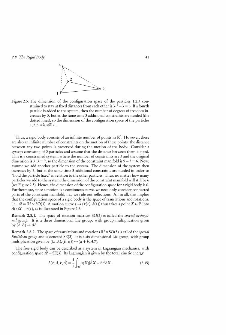
Figure 2.5: The dimension of the configuration space of the particles 1,2,3 con-strained to stay at fixed distances from each other is 3·3−3= 6. If a fourthparticle is added to the system, then the number of degrees of freedom in-creases by 3, but at the same time 3 additional constraints are needed (thedotted lines), so the dimension of the configuration space of the particles1,2,3,4 is still 6.
Thus, a rigid body consists of an infinite number of points in �3. However, thereare also an infinite number of constraints on the motion of these points: the distancebetween any two points is preserved during the motion of the body. Consider asystem consisting of 3 particles and assume that the distance between them is fixed.This is a constrained system, where the number of constraints are 3 and the originaldimension is 3 · 3= 9, so the dimension of the constraint manifold is 9− 3= 6. Now,assume we add another particle to the system. The dimension of the system thenincreases by 3, but at the same time 3 additional constraints are needed in order to“hold the particle fixed” in relation to the other particles. Thus, no matter how manyparticles we add to the system, the dimension of the constraint manifold will still be 6(see Figure 2.5). Hence, the dimension of the configuration space for a rigid body is 6.Furthermore, since a motion is a continuous curve, we need only consider connectedparts of the constraint manifold, i.e., we rule out reflections. All in all, this impliesthat the configuration space of a rigid body is the space of translations and rotations,i.e., Q =�3× SO(3). A motion curve t �→ (r (t ),A(t )) thus takes a point X ∈B intoA(t )X + r (t ), as is illustrated in Figure 2.6.
Remark 2.8.1. The space of rotation matrices SO(3) is called the special orthogo-nal group. It is a three dimensional Lie group, with group multiplication givenby (A,B) �→AB .
Remark 2.8.2. The space of translations and rotations�3×SO(3) is called the specialEuclidean group and is denoted SE(3). It is a six dimensional Lie group, with groupmultiplication given by ((a,A), (b,B)) �→ (a+ b,AB).
The free rigid body can be described as a system in Lagrangian mechanics, withconfiguration space Q = SE(3). Its Lagrangian is given by the total kinetic energy
L(r ,A, r , A) =1
2
∫B
ρ(X )|AX + r |2 dX , (2.35)
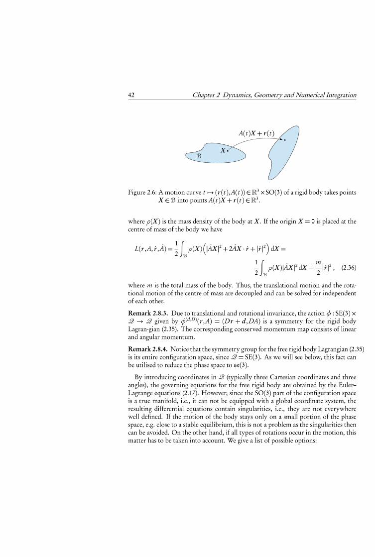
42 Chapter 2 Dynamics, Geometry and Numerical Integration
XB
A(t )X + r (t )
Figure 2.6: A motion curve t �→ (r (t ),A(t )) ∈�3×SO(3) of a rigid body takes pointsX ∈B into points A(t )X + r (t ) ∈�3.
where ρ(X ) is the mass density of the body at X . If the origin X = 0 is placed at thecentre of mass of the body we have
L(r ,A, r , A) =1
2
∫B
ρ(X )�|AX |2+ 2AX · r + |r |2
�dX =
1
2
∫B
ρ(X )|AX |2 dX +m
2|r |2 , (2.36)
where m is the total mass of the body. Thus, the translational motion and the rota-tional motion of the centre of mass are decoupled and can be solved for independentof each other.
Remark 2.8.3. Due to translational and rotational invariance, the action φ : SE(3)×Q → Q given by φ(d,D)(r ,A) = (D r + d, DA) is a symmetry for the rigid bodyLagran-gian (2.35). The corresponding conserved momentum map consists of linearand angular momentum.
Remark 2.8.4. Notice that the symmetry group for the free rigid body Lagrangian (2.35)is its entire configuration space, since Q = SE(3). As we will see below, this fact canbe utilised to reduce the phase space to se(3).
By introducing coordinates in Q (typically three Cartesian coordinates and threeangles), the governing equations for the free rigid body are obtained by the Euler–Lagrange equations (2.17). However, since the SO(3) part of the configuration spaceis a true manifold, i.e., it can not be equipped with a global coordinate system, theresulting differential equations contain singularities, i.e., they are not everywherewell defined. If the motion of the body stays only on a small portion of the phasespace, e.g. close to a stable equilibrium, this is not a problem as the singularities thencan be avoided. On the other hand, if all types of rotations occur in the motion, thismatter has to be taken into account. We give a list of possible options:
2.8 The Rigid Body 43
1. To reparametrise the SO(3)–part of the configuration space during the integra-tion of the governing equations. That is, to alternate between different coordinatecharts.
2. To embed the SO(3)–part in a larger dimensional vector space �n , where n > 3,and consider a corresponding constrained system. For example, by using quater-nions SO(3) may be embedded in �4. An embedding η : SO(3) → �n defines asubmanifold C ⊂ �n to which the solution is constrained. Thus, a constrained La-grangian system is obtained.
3. To utilise the fact that SO(3) is parallelisable (as is any Lie group). That is, itstangent bundle T SO(3) is isomorphic as a manifold to SO(3)× so(3). Indeed, anisomorphism is given by left translation of A to so(3)
T SO(3) � (A, A) �→ (A,LA−1∗A) = (A,A−1A) = (A, Ω) ∈ SO(3)× so(3) ,
where Ω is the body angular velocity, i.e., the angular velocity as seen from the bodyframe of reference. Alternatively one may use right translation
T SO(3) � (A, A) �→ (A,RA−1∗A) = (A, AA−1) = (A,ω) ∈ SO(3)× so(3) ,
where ω is the spatial angular velocity, i.e., the angular velocity as seen from thespatial frame of reference.
Remark 2.8.5. The Lie algebra so(3) is the space of skew symmetric 3× 3–matrices.Hence, it is isomorphic to�3. In accordance with standard notation, elements in so(3)are denoted with a hat, e.g. ω, and its corresponding element in �3 without the hat,e.g. ω. As so(3) is a matrix subgroup its Lie bracket is given by the matrix commu-tator [ω1,ω2] = ω1ω2− ω2ω1. The corresponding operation in �3 is given by thecross productω1×ω2. Furthermore, it holds that ω1ω2 =ω1×ω2.
Thus, elements (r ,A, r , A) in the phase space T SE(3) are isomorphic to elements(r , r ,A, Ω) in �3 ×�3 × SO(3)× so(3) (or to elements (r , r ,A,ω)). The whole ideawith the transformation is that so(3) is a vector space, so it can be equipped withglobal coordinates.
We now have to work out how the governing equations of motion look like ex-pressed in these elements. They will not have the Euler–Lagrange form due to thefact that the relation between A and Ω is not that of natural coordinates, i.e., in gen-eral (dA/dt )(t ) �= Ω(t ). For simplicity we only consider the rotational term in theLagrangian, as the translational term is trivial.
Due to the fact that the length of a vector is invariant under rotation and that theLagrangian is independent of A it holds that
L(A, A) = L(A) = L(BA) , ∀B ∈ SO(3).
44 Chapter 2 Dynamics, Geometry and Numerical Integration
This means that the kinetic rotational energy L is left invariant, i.e., it is invariantunder left translation LB∗. In turn, this implies that ∂ L/∂ A is left invariant, so that
∂ L
∂ A(A) = LA∗
� ∂ L
∂ Ω(Ω)
�=A∂ L
∂ Ω(Ω) . (2.37)
Due to (2.37) the Euler–Lagrange equations expressed in (A, Ω) instead of (A, A)transform according to
d
dt
∂ L
∂ A(A) =
∂ L
∂ A(A) = 0 ⇐⇒ d
dt
�A∂ L
∂ Ω(Ω)
�= 0
⇐⇒ Ad
dt
∂ L
∂ Ω(Ω)+ A
∂ L
∂ Ω(Ω) = 0 (2.38)
Since LA−1∗ is an isomorphism TASO(3) → so(3) we may apply it to the rightmostequation in (2.38), which gives
d
dt
∂ L
∂ Ω(Ω)+A−1A
∂ L
∂ Ω(Ω) = 0 ⇐⇒ d
dt
∂ L
∂ Ω(Ω)+ Ω
∂ L
∂ Ω(Ω) = 0 . (2.39)
Notice that these equations involve Ω, but not A. Thus, the phase space has been re-duced from T SO(3) to so(3). The equations (2.39) are actually the Euler equationsfor the free rotating rigid body.
From (2.36) it follows that L(Ω) is a positive definite quadratic form on so(3). Thus,it holds that �= ∂ L/∂ Ω is a linear invertible map so(3)→ so(3)∗ (its correspondingrepresentation on �3 is a symmetric positive definite matrix denoted �). In fact, it isthe inertia tensor of the rigid body. Expressed on �3 (i.e. transforming Ω �→ Ω) thegoverning equations (2.39) become
�Ω= �Ω×Ω . (2.40)
This is the classical form of the Euler equations. (We have used that Ω ∂ L∂ Ω(Ω) = Ω�Ω=
−�Ω×Ω.)When Ω(t ) has been computed then A(t ), i.e., the solution path on SO(3), is re-
constructed by the non-autonomous system A(t ) =A(t )Ω(t ).
Remark 2.8.6. From the second step in (2.38) it follows that
A∂ L
∂ Ω(Ω) (which expressed on �3 is A�Ω)
is conserved by the flow. From a Noether’s theorem point of view, this is the con-served momentum map (angular momentum) due to invariance of the Lagrangianwith respect to left action of the symmetry group SO(3).
2.9 Hamiltonian Mechanics 45
Remark 2.8.7. The inertia tensor � induces an Euclidean structure on so(3) by
(ω1,ω2) �→ ⟨�(ω1),ω2⟩.In turn, this structure induces a left invariant Riemannian metric on SO(3) by lefttranslation. Arnold pointed out in his ground breaking paper [4] that motions of thefree rigid body correspond to geodesics on SO(3) with respect to this induced Rie-mannian metric. The results were also generalised to infinite dimensional Lie groups,with a particular application to the hydrodynamics of ideal fluids. Arnold’s paperwas the starting point for the theory of mechanics on Lie groups and topologicalfluid dynamics, see [34].
So far we have derived the governing equations for the free rigid body. In presenceof orientation and translation dependent forces and moments, the full set of govern-ing equations (expressed using Ω) take the form
m r = F
�Ω= �Ω×Ω+M
A=AΩ ,
(2.41)
where F and M are the forces and moments respectively acting on the body. Theseequations are sometimes called the Newton–Euler equations.
2.9 Hamiltonian Mechanics
A Lagrangian mechanical system is defined by a configuration manifold Q and La-grangian function. As we have seen, the principles and the form of the governingequations in Lagrangian mechanics are invariant with respect to transformations be-tween local coordinates in Q, or, if one likes, with respect to the group of diffeomor-phisms on Q. We are not, however, free to choose any coordinates on TQ: they mustbe the induced natural coordinates.
In Hamiltonian mechanics, a system is defined by a symplectic manifold P of di-mension 2n and a function H : P→� on it. The principles and the governing equa-tions in Hamiltonian mechanics are invariant with respect to all diffeomorphismson P that preserve the symplectic structure. Notably, this group of transformationsis larger than Diff(Q).
2.9.1 Symplectic Manifolds
Definition 2.9.1. A symplectic manifold is a differential manifold P together with anon-degenerate closed differential 2–form Ω on it.
46 Chapter 2 Dynamics, Geometry and Numerical Integration
Recall that a differential 2–form on a manifold is a field of skew symmetric bilinearforms (one on each tangent space). That is, to each tangent space TzP , a bilinear skewsymmetric form Ω(z) : TzP ×TzP → � is associated. Just as an inner product on avector space E induces an isomorphism E→ E∗, the form Ω(z), being non-degenerate,induces an isomorphism J(z) : TzP→ T ∗
zP by
J(z) : v �→Ω(z)[·,v] . (2.42)
Definition 2.9.2. A map ϕ : P→P is called symplectic (or sometimes canonical) ifit preserves the symplectic form Ω. That is ϕ∗Ω=Ω.
Remark 2.9.1. Recall that the pullback ϕ∗Ω of differential 2–forms is defined by
(ϕ∗Ω)(z)[v,w] = Ω(ϕ(z))[ϕ∗(z)v,ϕ∗(z)w] .
Remark 2.9.2. Recall that a 2–form is called closed if its exterior derivative is zero,i.e., dω = 0. Due to Poincaré’s lemma and Darboux’s theorem, the symplectic formbeing closed implies that locally there exists a coordinate chart in which Ω has thecanonical representation Ω= dq ∧ dp. See [38, Ch. 5] for details.
Remark 2.9.3. From standard properties of the determinant one gets
det(J(z)) = det(J(z)∗) = det(−J(z)) = (−1)m det(J(z)),
where m is the dimension of P . Since J(z) is non-singular, this implies that a sym-plectic manifold must be even dimensional, i.e., m = 2n for some positive integern.
2.9.2 Hamiltonian Vector Fields and Phase Flows
A Hamiltonian system is defined by a symplectic manifold P , called the phase space,and a real valued function H on it. The corresponding Hamiltonian vector field isgiven by
XH (z) = J(z)−1 dH (z) .
Thus, the governing equations of motion for a Hamiltonian system are given by
dz
dt=XH (z) . (2.43)
The solution curves as a function of the initial data is a map ϕ t : P →P called thephase flow. Notice that ϕ indeed is a flow, i.e., it fulfils ϕ t ◦ϕ s = ϕ t+s .
Remark 2.9.4. As in Lagrangian mechanics, the Hamiltonian function may also de-pend explicitly on time t , so non-autonomous systems may also be treated. In thefollowing, we will assume that every system is autonomous. This is not actually a re-striction, as the phase space may be extended to include also time and a correspondingmomentum variable, see [50]
2.9 Hamiltonian Mechanics 47
Recall the following properties of Hamiltonian systems:
1. The Hamiltonian function H is a first integral, i.e., energy is conserved. Indeed,
dH (z)
dt= ⟨dH (z),
dz
dt⟩= ⟨J(z)XH (z),XH (z)⟩=Ω(z)[XH (z),XH (z)] = 0 ,
where the last equality follows from the skew symmetry of Ω. As a straightfor-ward generalisation of this result, notice that any real valued function I on Psuch that Ω[XI ,XH ] = 0 is a first integral of (2.43).
2. The phase flow ϕ t , with fixed t , is a symplectic map P →P . See Arnold [5,Ch. 8] for a proof.
Remark 2.9.5. The symplectic form induces a bilinear map F(P)×F(P)→ F(P)by
{H , I }(z) = Ω(z)[XI (z),XH (z)] (2.44)
called the Poisson bracket. Thus, I is a first integral of the Hamiltonian system withHamiltonian function H if and only if {H , I }= 0.
Due to the fact that Ω is closed, it holds that X{H ,I } = [XH ,XI ]. Thus, the Poissonbracket (2.44) gives F(P) the structure of a Lie algebra. By the homomorphism F �→XF this algebra defines a Lie subalgebra of X(P) called the Lie algebra of Hamiltonianvector fields and denoted XΩ(P). The corresponding infinite dimensional sub-groupof Diff(P) is the group of symplectic transformation and is denoted DiffΩ(P).
2.9.3 Canonical Symplectic Structure on T ∗Q and the LegendreTransformation
As mentioned before, coordinates q on Q induce canonical coordinates z = (q, p) onT ∗Q, such that an element in T ∗q Q is represented by p dq. Now, notice that p dq canbe interpreted as a differential 1–form θ on T ∗Q, i.e., a field of forms Tz T ∗Q→ �.θ is called the canonical 1–form on T ∗Q. Its exterior derivativeω = dθ defines a non-degenerate 2–form on T ∗Q called the canonical symplectic form. In coordinates wehave that ω = dp ∧ dq. Hence, the manifold T ∗Q equipped with ω is a symplecticmanifold.
Expressed in canonical coordinates, the map (2.42) is given by
J =�
0 −IdId 0
�.
48 Chapter 2 Dynamics, Geometry and Numerical Integration
Thus, the governing equations dz/dt = J−1∇H (z ) expressed in canonical coordi-nates for a Hamiltonian system on T ∗Q have the form
dq
dt=∂ H (q, p)
∂ pdp
dt=−∂ H (q, p)
∂ q.
(2.45)
The relation between Lagrangian and Hamiltonian mechanics is via the Legendretransformation, which takes a Lagrangian system on TQ and transforms it into aHamiltonian system on T ∗Q. It is defined by the map
TQ � vq �→d
dε
ε=0
L(vq+ ε · ) ∈ T ∗Q . (2.46)
In natural coordinates on TQ and corresponding canonical coordinates on T ∗Q ittakes the form
(q, q) �→�
q,∂ L(q, q)
∂ q
�= (q, p) . (2.47)
Notice that this is an isomorphism if and only if q is a well defined function of (q, p),i.e., if ∂ L(q, q)/∂ q as a map TqQ→ T ∗q Q is invertible. Such Lagrangians are calledregular.
For a Lagrangian system with a regular Lagrangian function, the Legendre trans-formation takes the Euler–Lagrange equations (2.17) into a Hamiltonian system withHamiltonian function H (q, p) = p · q − L(q, q).
2.9.4 Poisson Dynamics
Poisson dynamics is a generalisation of symplectic dynamics. The idea is to startdirectly with Poisson bracket which is not necessarily of the form (2.44). Instead, Pis called a Poisson manifold if it is equipped with a Poisson bracket, which is a bilinearmap {·1, ·2} : F(P)×F(P)→ F(P) that fulfils
{F ,G}=−{G, F } (skew-symmetry) (2.48a){F G, H}= F {G, H}+G{F , H} (Leibniz rule) (2.48b){{F ,G}, H}+ {{H , F },G}+ {{G, H}, F }= 0 (Jacobi identity) . (2.48c)
A Poisson system is a dynamical system determined by the Poisson structure and aHamiltonian function H ∈ F(P). The equations of motion are given by
dF
dt= {H , F } , ∀ F ∈ F(P) . (2.49)
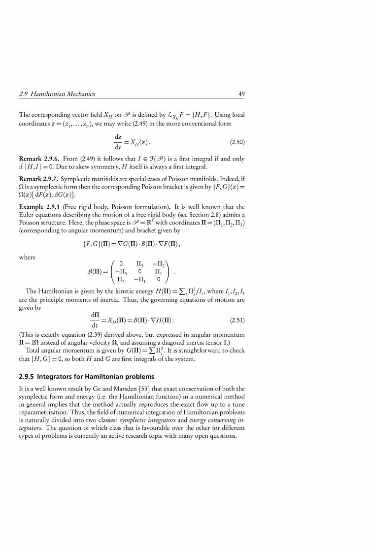
2.9 Hamiltonian Mechanics 49
The corresponding vector field XH on P is defined by LXHF = {H , F }. Using local
coordinates z = (z1, . . . , zn), we may write (2.49) in the more conventional form
dz
dt=XH (z ) . (2.50)
Remark 2.9.6. From (2.49) it follows that I ∈ F(P) is a first integral if and onlyif {H , I }= 0. Due to skew symmetry, H itself is always a first integral.
Remark 2.9.7. Symplectic manifolds are special cases of Poisson manifolds. Indeed, ifΩ is a symplectic form then the corresponding Poisson bracket is given by {F ,G}(z ) =Ω(z )[dF (z ), dG(z )].
Example 2.9.1 (Free rigid body, Poisson formulation). It is well known that theEuler equations describing the motion of a free rigid body (see Section 2.8) admits aPoisson structure. Here, the phase space is P =�3 with coordinatesΠ= (Π1,Π2,Π3)(corresponding to angular momentum) and bracket given by
{F ,G}(Π) =∇G(Π) ·B(Π) · ∇F (Π) ,
where
B(Π) =
⎛⎜⎝ 0 Π3 −Π2−Π3 0 Π1Π2 −Π1 0
⎞⎟⎠ .
The Hamiltonian is given by the kinetic energy H (Π) =∑
i Π2i /Ii , where I1, I2, I3
are the principle moments of inertia. Thus, the governing equations of motion aregiven by
dΠdt=XH (Π) = B(Π) · ∇H (Π) . (2.51)
(This is exactly equation (2.39) derived above, but expressed in angular momentumΠ= �Ω instead of angular velocity Ω, and assuming a diagonal inertia tensor �.)
Total angular momentum is given by G(Π) =∑Π2
i . It is straightforward to checkthat {H ,G}= 0, so both H and G are first integrals of the system.
2.9.5 Integrators for Hamiltonian problems
It is a well known result by Ge and Marsden [53] that exact conservation of both thesymplectic form and energy (i.e. the Hamiltonian function) in a numerical methodin general implies that the method actually reproduces the exact flow up to a timereparametrisation. Thus, the field of numerical integration of Hamiltonian problemsis naturally divided into two classes: symplectic integrators and energy conserving in-tegrators. The question of which class that is favourable over the other for differenttypes of problems is currently an active research topic with many open questions.
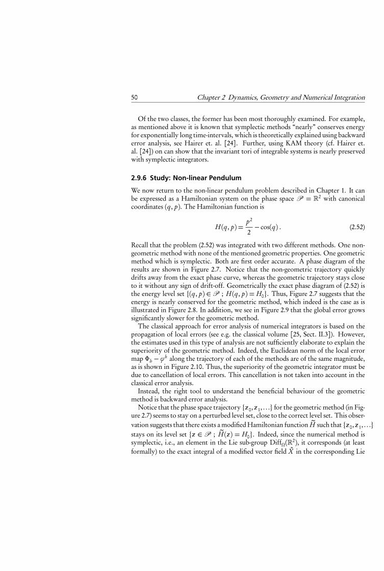
50 Chapter 2 Dynamics, Geometry and Numerical Integration
Of the two classes, the former has been most thoroughly examined. For example,as mentioned above it is known that symplectic methods “nearly” conserves energyfor exponentially long time-intervals, which is theoretically explained using backwarderror analysis, see Hairer et. al. [24]. Further, using KAM theory (cf. Hairer et.al. [24]) on can show that the invariant tori of integrable systems is nearly preservedwith symplectic integrators.
2.9.6 Study: Non-linear Pendulum
We now return to the non-linear pendulum problem described in Chapter 1. It canbe expressed as a Hamiltonian system on the phase space P = �2 with canonicalcoordinates (q , p). The Hamiltonian function is
H (q , p) =p2
2− cos(q) . (2.52)
Recall that the problem (2.52) was integrated with two different methods. One non-geometric method with none of the mentioned geometric properties. One geometricmethod which is symplectic. Both are first order accurate. A phase diagram of theresults are shown in Figure 2.7. Notice that the non-geometric trajectory quicklydrifts away from the exact phase curve, whereas the geometric trajectory stays closeto it without any sign of drift-off. Geometrically the exact phase diagram of (2.52) isthe energy level set {(q , p) ∈P ; H (q , p) = H0}. Thus, Figure 2.7 suggests that theenergy is nearly conserved for the geometric method, which indeed is the case as isillustrated in Figure 2.8. In addition, we see in Figure 2.9 that the global error growssignificantly slower for the geometric method.
The classical approach for error analysis of numerical integrators is based on thepropagation of local errors (see e.g. the classical volume [25, Sect. II.3]). However,the estimates used in this type of analysis are not sufficiently elaborate to explain thesuperiority of the geometric method. Indeed, the Euclidean norm of the local errormap Φh −ϕh along the trajectory of each of the methods are of the same magnitude,as is shown in Figure 2.10. Thus, the superiority of the geometric integrator must bedue to cancellation of local errors. This cancellation is not taken into account in theclassical error analysis.
Instead, the right tool to understand the beneficial behaviour of the geometricmethod is backward error analysis.
Notice that the phase space trajectory {z 0, z 1, . . .} for the geometric method (in Fig-ure 2.7) seems to stay on a perturbed level set, close to the correct level set. This obser-vation suggests that there exists a modified Hamiltonian function �H such that {z 0, z 1, . . .}stays on its level set {z ∈P ; �H (z ) = H0}. Indeed, since the numerical method issymplectic, i.e., an element in the Lie sub-group DiffΩ(�2), it corresponds (at leastformally) to the exact integral of a modified vector field X in the corresponding Lie
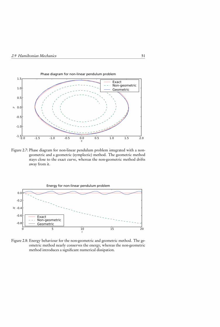
2.9 Hamiltonian Mechanics 51
Phase diagram for non-linear pendulum problem
-2.0 -1.5 -1.0 -0.5 0.0 0.5 1.0 1.5 2.0q
-1.5
-1.0
-0.5
0.0
0.5
1.0
1.5
p
ExactNon-geometricGeometric
Figure 2.7: Phase diagram for non-linear pendulum problem integrated with a non-geometric and a geometric (symplectic) method. The geometric methodstays close to the exact curve, whereas the non-geometric method driftsaway from it.
Energy for non-linear pendulum problem
0 5 10 15 20t
-0.8
-0.6
-0.4
-0.2
0.0
H
ExactNon-geometricGeometric
Figure 2.8: Energy behaviour for the non-geometric and geometric method. The ge-ometric method nearly conserves the energy, whereas the non-geometricmethod introduces a significant numerical dissipation.
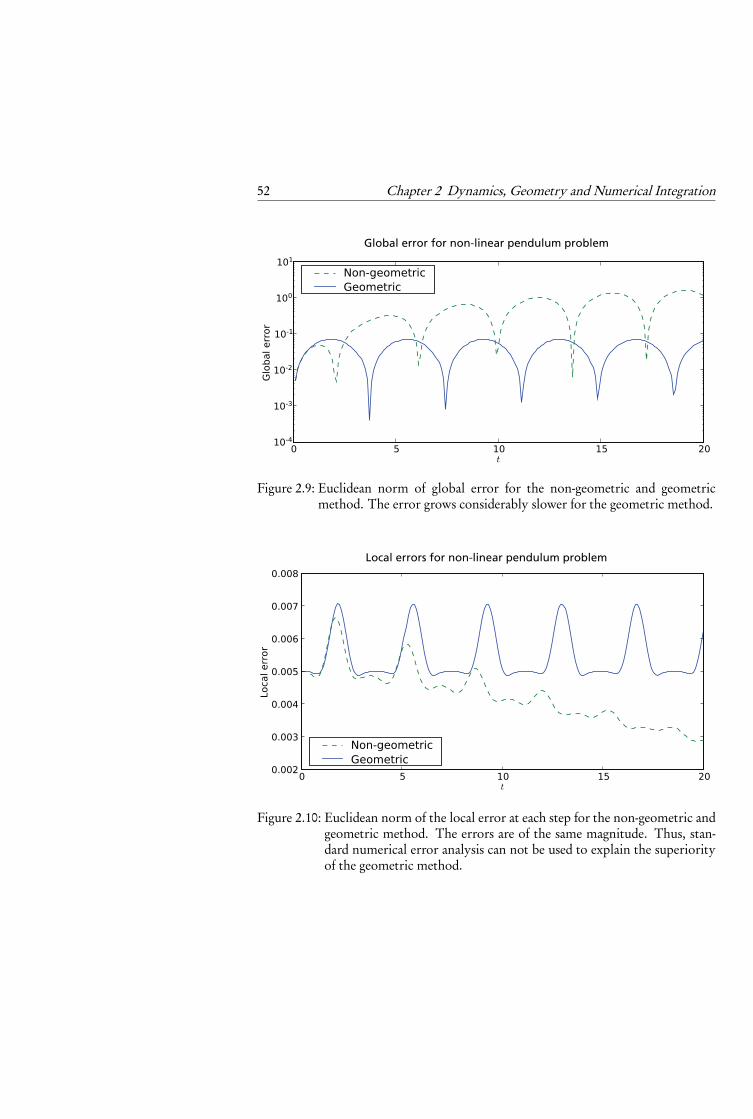
52 Chapter 2 Dynamics, Geometry and Numerical Integration
Global error for non-linear pendulum problem
0 5 10 15 20t
10-4
10-3
10-2
10-1
100
101G
lobal err
or
Non-geometricGeometric
Figure 2.9: Euclidean norm of global error for the non-geometric and geometricmethod. The error grows considerably slower for the geometric method.
Local errors for non-linear pendulum problem
0 5 10 15 20t
0.002
0.003
0.004
0.005
0.006
0.007
0.008
Loca
l err
or
Non-geometricGeometric
Figure 2.10: Euclidean norm of the local error at each step for the non-geometric andgeometric method. The errors are of the same magnitude. Thus, stan-dard numerical error analysis can not be used to explain the superiorityof the geometric method.
2.10 Nambu Mechanics 53
sub-algebra XΩ(�2). Since XΩ(�2) is isomorphic as a Lie algebra, up to a constant, toF(�2) equipped with the Poisson bracket, it holds that every vector field in XΩ(�2)is generated by corresponding Hamiltonian function in F(�2). Thus, z = X (z ) is aHamiltonian system for a modified Hamiltonian function H .
2.10 Nambu Mechanics
In Hamiltonian mechanics, the phase space manifold P is equipped with a Poissonstructure, defined by a bracket operation {·1, ·2} : F(P) × F(P) → F(P) that isskew-symmetric, fulfils the Leibniz rule and the Jacobi identity. Nambu–Poissonmechanics is a generalisation.
Definition 2.10.1. A Nambu–Poisson manifold of order k consists of a smooth man-ifold P together with a multilinear map
{·1, . . . , ·k} : F(P)× . . .×F(P)︸ ︷︷ ︸k times
→ F(P)
that fulfils:
• total skew-symmetry
{H1, . . . , Hk}= sgn(σ){Hσ1, . . . , Hσk
} (2.53a)
• Leibniz rule
{GH1, . . . , Hk}=G{H1, . . . , Hk}+H1{G, H2, . . . , Hk} (2.53b)
• fundamental identity
{H1, . . . , Hk−1,{G1, . . . ,Gk}}= {{H1, . . . , Hk−1,G1},G2, . . . ,Gk}+ {G1,{H1, . . . , Hk−1,G2},G3, . . . ,Gk}+ . . .+ {G1, . . . ,Gk−1,{H1, . . . , Hk−1,Gk}}.
(2.53c)
Remark 2.10.1. The case k = 2 coincides with ordinary Poisson manifolds.
The first two conditions, total skew-symmetry (2.53a) and Leibniz rule (2.53b), arestraightforward: they imply that the bracket is of the form
{H1, . . . , Hk}= η(dH1, . . . , dHk )
for some totally skew-symmetric contravariant k–tensor η [51]. The third condition,the fundamental identity (2.53c), is more intricate. The range of possible Poisson–Nambu brackets is heavily restricted by this condition [51].

54 Chapter 2 Dynamics, Geometry and Numerical Integration
A Nambu–Poisson system on a Nambu–Poisson manifold of order k is determinedby k − 1 Hamiltonian function H1, . . . , Hk−1 ∈ F(P). The governing equations are
dF
dt= {H1, . . . , Hk−1, F } ∀ F ∈ F(P), (2.54a)
which may also be writtendx
dt=XH1,...,Hk−1
(x), (2.54b)
where XH1,...,Hk−1∈ X(P) is defined by LXH1,...,Hk−1
F = {H1, . . . , Hk−1, F }. The cor-responding flow map is denoted ϕ t
H1,...,Hk−1. Notice that due to skew symmetry of
the bracket, all the Hamiltonians H1, . . . , Hk−1 are first integrals, which follows fromequation (2.54a).
Due to the fundamental identity (2.53c), Nambu–Poisson systems fulfil certainproperties which have direct counterparts in Hamiltonian mechanics (the case k = 2).
Theorem 2.10.1 (Takhtajan [51]). The set of first integrals of system (2.54) is closed un-der the Nambu–Poisson bracket. That is, if G1, . . . ,Gk are first integrals, then {G1, . . . ,Gk}is again a first integral.
Theorem 2.10.2 (Takhtajan [51]). The flow of system (2.54) preserves the Nambu–Poisson structure. That is,
{G1, . . . ,Gk}◦ϕ tH1,...,Hk−1
= {G1◦ϕ tH1,...,Hk−1
, . . . ,Gn◦ϕ tH1,...,Hk−1
} ∀G1, . . . ,Gk ∈ F(P),
or equivalentlyLXH1,...,Hk−1
η= 0. (2.55)
Remark 2.10.2. The set of vector fields that fulfils equation (2.55) is denoted Xη(P).Clearly Xη(P) is closed under linear combinations, so it is a sub-space of X(P).Further, since L[X ,Y ]η = LX (LYη)−LY (LXη) it is also closed under the com-mutator. Thus, Xη(P) is a Lie sub-algebra of X(P). Correspondingly, Diffη(P)denotes the Lie sub-group of Diff(P) that preserves the Nambu–Poisson structure.An element Φ ∈ Diffη(P) is called an η–map.
Remark 2.10.3. It is important to point out that in general not every X ∈ Xη(P)corresponds to a Nambu–Poisson system, i.e., a system of the form of equation (2.54).The reason is that the set of vector fields of the form of equation (2.54) is not closedunder linear combinations.
There are also fundamental differences between Hamiltonian and Nambu–Poissonmechanics, i.e., between k = 2 and k ≥ 3. In particular there is the following result,conjectured by Chatterjee and Takhtajan [11] and later proved by several authors.
2.10 Nambu Mechanics 55
Theorem 2.10.3 ([17], [3], [43], [31], [36]). A totally skew-symmetric contravarianttensor of order k ≥ 3 is a Nambu–Poisson tensor if and only if it is locally decomposableabout any regular point. That is, about any point x ∈P such that η(x) �= 0 there existlocal coordinates (x1, . . . , xk , xk+1, . . . , xn) such that
η=∂
∂ x1∧ · · · ∧ ∂
∂ xk.
Thus, every Nambu–Poisson tensor with k ≥ 3 is in essence a determinant on asub-manifold of dimension k. It is not so for Poisson tensors.
In Paper IV geometric Nambu–Poisson integrators are obtained by splitting of eachif the Nambu Hamiltonians. Thus, these integrators have the geometric property thatthey preserve the Nambu–Poisson tensor.

56 Chapter 2 Dynamics, Geometry and Numerical Integration
Chapter 3
Time Transformation and Adaptivity
Time is no law of nature. It is a plan. When you look at it withawareness, or start to touch it, then it starts to disintegrate.
(Peter Høeg, “Borderliners”)
As mentioned in the introduction, the approach to adaptivity for geometric integra-tors is to introduce a time reparametrisation t↔ τ in the governing equations suchthat the flow ψτ of the transformed system corresponds to the flow ϕ t of the originalsystem by
ψτ(z ) = ϕσ(τ,z )(z ) ,
where σ(·, z ) is a bijective function �→ � for each z in the phase space. The ideais then to discretise the time transformed governing equations with a geometric inte-grator, using equidistant steps ε in τ, which correspond to variable steps in t .
Different types of time transformation techniques have been used. Below we re-view them, and point out how they are used to construct adaptive integrators withgeometric properties.
3.1 Sundman Transformation
Consider a dynamical system with phase space P on the form
dz
dt=X (z ) . (3.1)
Reparametrisation of time t↔ τ in (3.1) yields an equivalent time transformed sys-tem
dz
dτ=
dt
dτX (z ) . (3.2)
A Sundman transformation is a time transformation where the relation between tand τ is determined dynamically by a relation on the form dt/dτ =G(z ). The realvalued function G is called the scaling function of the time transformation, and is
57
58 Chapter 3 Time Transformation and Adaptivity
assumed to be strictly positive, thus making the transformation bijective. Altogether,a new dynamical system is obtained
dz
dτ=G(z )X (z ) (3.3a)
dt
dτ=G(z ) . (3.3b)
Notice that it is an autonomous system on the extended phase space P � withcoordinates (z , t ). Since the original system is autonomous (3.3b) does not alter (3.3a),so dynamics is restricted to P . Reconstruction of time (3.3b) is merely quadrature.
Sundman transformations have been used to construct reversible/symmetric adap-tive integrators, see [49, 29, 9]. However, if X is symplectic, the transformed vectorfield G(z )X (z ) is not in general symplectic. For this reason the Sundman transfor-mation has not been used to construct adaptive symplectic methods. Nevertheless,it turns out that by using a splitting technique in conjunction with Sundman trans-formations, it is possible to preserve symplecticity. This approach is investigated inPaper II of the thesis.
3.2 Extended Phase Space Approach
In this section we review the explicit reversible step size control suggested in [26].Consider a reversible Hamiltonian system on a symplectic phase space P with
canonical coordinates z = (q, p). That is, a system on the form
dz
dt=XH (z ) (3.4)
where the Hamiltonian vector field XH is reversible with respect to the linear map
R : (q, p) �→ (q,−p) .
That is,R ◦XH =−XH ◦R.
Due to the reversibility condition the flow ϕ tXH
is reversible, i.e., R ◦ϕ tXH= ϕ−t
XH◦R.
In order to obtain time step adaptivity, the time variable t is considered as a func-tion of a new independent variable τ. Let the step density ρ be defined by dt/dτ =1/ρ. Hence we have d/dt = ρd/dτ. The idea is now to determine the step sizecontrol by specifying an equation on the form dρ/dτ = ξ (z ) for the step density.Here, ξ : P → � determines the dynamics of the step size control. Substituting
3.3 Nambu Mechanics and Time Transformation 59
d/dt = ρd/dτ in (3.4) and adding the equation for ρ we end up with an augmenteddynamical system
dz
dτ=XH (z )/ρ
dρ
dτ= ξ (z )
(3.5)
on the extended phase space P = P ×� with coordinates z = (z ,ρ). Just as forSundman transformations, notice that the time variable t does not alter the dynamicsof (3.5); it is recovered by a mere quadrature process. If ξ fulfils ξ =−ξ ◦R then theaugmented system (3.5) is reversible with respect to the map R : (z ,ρ) = (R(z ),ρ).
Typical adaptivity aims at keeping the step size times a positive function Q : P→�+, called a control objective, constant. That is, Q(z )/ρ= const. By differentiatingthat objective we are lead to
ξ (z ) = {Q, H}(z )/Q(z ). (3.6)
This choice fulfils the reversibility condition on ξ whenever Q =Q ◦R.In [26] the following algorithm is suggested.
Algorithm 3.2.1. Let Φh be a reversible one-step method for (3.4). Further, let ρ0 =1, and let ε > 0 be a constant. Define z 0, z 1, . . . by
ρk+1/2 = ρk + εξ (z k )/2 ,
z k+1 =Φε/ρk+1/2(z k ) ,
ρk+1 = ρk+1/2+ εξ (z k )/2 ,
(3.7)
where z k approximates z (tk ) and time is reconstructed by tk+1 = tk + ε/ρk+1/2.
This defines a reversible (with respect to R) one-step method Φε for (3.5). In par-ticular, if the Hamiltonian is separable H (z ) = T (p) +V (q) and Φh is the Störmer–Verlet method, then Φε gives a fully explicit adaptive reversible integrator of order 2.
Just as in the Sundman transformation case, symplecticity is not preserved by stepdensity transformations, so Φε is not a symplectic integrator although Φh is.
3.3 Nambu Mechanics and Time Transformation
In this section we review the time transformation technique for Nambu–Poisson sys-tems developed in Paper IV. By splitting of the individual Nambu Hamiltonians, thistechnique can be used to construct adaptive integrators that preserve the Nambu–Poisson structure.
60 Chapter 3 Time Transformation and Adaptivity
Let P be a Nambu–Poisson manifold of order k and η its Nambu–Poisson tensor.Consider again the extended phase space P =P×�. Our first goal is to introduce aNambu–Poisson structure on P . The most natural extension of the Nambu–Poissontensor η is given by
η= η∧ ∂∂ ξ
. (3.8)
It is not obvious that the bracket corresponding to η will fulfil the fundamental iden-tity (2.53c). For example, in the canonical Poisson case, i.e., k = 2, it is not so ifn ≥ 3.
Lemma 3.3.1. If k ≥ 3 or k = n = 2, then η given by equation (3.8) defines a Nambu–Poisson structure of order k + 1 on P .
Proof. If k ≥ 3 then it follows from Theorem 2.10.3 that η is decomposable aboutits regular points, and when k = n = 2 it is obviously so. Thus, η ∧ ∂
∂ ξis also
decomposable about its regular points, so the assertion follows from Theorem 2.10.3.
The bracket associated with η is denoted {·, . . . , ·}.Let H1, . . . , Hk−1 ∈ F(P) be the Hamiltonians for a Nambu–Poisson system on
P , i.e., of the form of system (2.54). Further, let G ∈ F(P) and consider the systemon P given by
dF
dτ= {H1, . . . , Hk−1,G, F } ∀ F ∈ F(P). (3.9)
Remark 3.3.1. A functions H ∈ F(P) is considered to belong to F(P) by the natu-ral extension x �→H (x). Likewise, H ∈ F(P) is considered to be a function in F(P)depending on the parameter ξ . Thus, {·, . . . , ·} is defined also for elements in F(P)and vice versa.
The following is a main result in Paper IV. It states that time transformation of aNambu–Poisson system can be realised as an extended Nambu–Poisson system.
Theorem 3.3.1. Let G ∈ F(P) and assume the conditions in Lemma 3.3.1 are valid.Then:
1. The extended system (3.9) is a Nambu–Poisson system.
2. Its flow restricted to P is a time transformation, determined by the additional firstintegral G, of the flow of system (2.54). That is,
ΠϕτH1,...,Hk−1,G(x) = ϕσ(τ,x)H1,...,Hk−1
(x) ∀ x ∈ P ,τ ∈�,

3.3 Nambu Mechanics and Time Transformation 61
where
σ(τ, x)≡∫ τ
0
∂ G
∂ ξ
�ϕ s
H1,...,Hk−1,G(x)�
ds .
Proof. The first assertion follows directly from Lemma 3.3.1, since η is a Nambu–Poisson tensor. Since Hi for i = 1, . . . , k−1 are independent of ξ , it follows from thedefinition (3.8) of η that
{H1, . . . , Hk−1,G, F }= ∂ G
∂ ξ{H1, . . . , Hk−1, F }− ∂ F
∂ ξ{H1, . . . , Hk−1,G}.
Thus, for F = x1, . . . , xn , the governing equations (3.9) are parallel with those of sys-tem (2.54a), i.e., ΠϕτH1,...,Hk−1,G and ϕ t
H1,...,Hk−1defined the same phase diagram. The
relation between τ and t is given by dt/dτ = ∂ G/∂ ξ , which, after integration,gives the desired form of σ(τ, x).
It is straightforward to check the following corollary, which shows that the tech-nique used by Hairer and Söderlind [26], reviewed in Section 3.2, is a special case.
Corollary 3.3.1. The case G(x) = log(ξ /Q(x)) coincides with the transformation (3.5)applied to system (2.54).

62 Chapter 3 Time Transformation and Adaptivity
Chapter 4
Implementation
Things should be made as simple as possible, but not any simpler.
(Albert Einstein)
4.1 Multibody Problems
In this section we discuss numerical issues that are specific to multibody problemswith contact force laws between bodies.
Consider a system of N bodies. We assume that the configuration space for body ihas the form
Qi = SE(3)×Vi . (4.1)
• SE(3) is the natural configuration space for a rigid body (recall Section 2.8). Itdescribes the position and orientation of the centre of mass of the body.
• Vi is a vector space that describes additional degrees of freedom for the body,e.g. elasticity and/or thermal distribution. If body i is rigid, then Vi is theempty set.
In practical numerical computations some coordinate representation must be usedfor the phase space T Qi . Recall from Section 2.8 that there are various ways of doingthis. The approach we consider here is to use parallelisability of SE(3). Thus, thephase space for body i is Pi = SE(3)× se(3)× Vi × Vi (since Vi is a vector space).Global coordinates may be introduced in the se(3)×Vi ×Vi part of the phase space(the vector space part). However, we also need to represent elements in SE(3), whichis not a vector space since it contains SO(3). As mentioned in Section 2.8 quater-nions may be used to embed SO(3) in �4. It is essential that the numerical solutionstays at the sub-manifold induced by the embedding. A natural way of achievingthis is to use so called Lie group integrators. These integrators are based on the factthat SO(3) is closed under matrix multiplication. For an extensive treatment of thetheory, see [32].
63
64 Chapter 4 Implementation
The governing differential equations for a system of N bodies are on the form
dz i
dt=Xi (z
i )+∑j �=i
Xi j (zi , z j ) , (4.2)
where
• z i ∈Pi are state variables for body i ,
• Xi : Pi → T Pi describes the internal dynamics of body i ,
• Xi j : Pi ×P j → T Pi describes the dynamics due to interaction betweenbody i and body j .
4.1.1 Constraints and impact force laws
In computational multibody mechanics the treatment of constraints is a crucial issue,although not the main focus in this thesis. In addition to the obvious possibility ofreducing the dynamics to the constraint manifold in accordance with (2.21), there aretwo main principles:
1. To solve the augmented set of governing equations (2.22), which has the formof a differential algebraic equation (DAE). Usually this approach involves a re-formulation of the governing DAE in order to lower its index. See [16, 35] forfurther details.
2. To add a strong penalty potential, which forces the system to stay on the con-straint manifold. The introduction of a penalty potential makes the problemhighly stiff, which implies that implicit methods are necessary for stability iflarge time steps are to be used.
Remark 4.1.1. In the multibody software package BEAST constraints are typicallymodelled as stiff spring–dampers, i.e., the second approach.
For the multibody application we have in mind, the interaction dynamics betweenbody i and body j take the form
Xi j =X Ci j +X F
i j , (4.3)
where:
• X Ci j is due to penalty constraint forces. Thus, it is of a stiff character, mean-
ing that the aimed step size lengths are not small enough to fully resolve thedynamics it gives rise to.
4.2 Library implemented in BEAST 65
• X Fi j describes the dynamics due to impact and contact forces between body i
and j . Such forces are highly complex, and computing them typically requiresa search for intersecting surfaces between the bodies, which is computationallyexpensive. Indeed, in an application such as BEAST these forces are significantlymore expensive to evaluate than other types of forces.
The stiff character of the system, due to penalty constraint forces, implies that im-plicit methods must be used. From an efficiency point of view a standard implicitmethod is, per time step, more computationally expensive than an explicit ditto, be-cause at each time step a non-linear equation needs to be solved iteratively. In partic-ular, this implies that the right hand side vector field is evaluated several times eachstep.
In Paper V of the thesis, mechanical multibody systems with governing equationson the form
dz
dt=XA(z )+XB (z ) ,
are considered. XA is expensive to evaluate, but non-stiff. XB is inexpensive to evalu-ate, but stiff. A class of integration methods for such problems is suggested. Theseintegrators are “explicit in XA and implicit in XB ” in the sense that XA is only eval-uated once per step (or two depending on the order), and its Jacobian matrix is notneeded. Thus, if XA is dominating the computational cost, then the proposed integra-tors are as efficient per time step as standard explicit integrators, but still allow largestep sizes to be used, due to the implicit handling of the stiff part XB . Consistency andlinear stability analysis of the proposed methods are also investigated in the paper.
4.2 Library implemented in BEAST
Based on variational integrators, and on the research in Paper I–V, a software libraryfor numerical integration of multibody problems has been implemented in C++. Withan object oriented class design, the library is built to be as modular as possible. Theprinciple base classes are:
Body
An object from this class represents a body in the system with a phase space on theform (4.1). Member variables include state representation of the body (i.e. a coordi-nate representation of an element in Pi ) as well as other body specific parameterssuch as mass and moments of inertia.
BodyForce
Base class for an object that represents an external force acting on one body, e.g. grav-ity. A reference to the body object is held. There is also a method for computing the
66 Chapter 4 Implementation
force acting on the body when it is in its current state.
ConnectionForce
Base class for a force acting between two bodies, e.g. a contact force. References toboth bodies are held, and a method for computing the force.
SystemIntegrator
An object from this class represents a full multibody system and a one step integra-tion method used to solve the system. Member variables include a list of Body objects,a list of BodyForce objects, and a list of ConnectionForce objects. There is a stepmethod, that advances the system from its current to its next state.
The advantage with this library design, over general purpose ODE–solver libraries,is that it allows the integration algorithms (SystemIntegrator subclasses) to be“aware” of the structure of the multibody system. For example, each force object(BodyForce or ConnectionForce) has a flag that specifies if it is expensive or not toevaluate (in accordance with the previous section), and a flag for whether or not it isconservative. Yet, its design is not specific to a particular multibody software code.This allows for simple and generic implementation of integration methods, wheresystem specific structures can be utilised to increase efficiency.
A SystemIntegrator subclass with the following properties has been implemented:
• The basic integration scheme is based on the method suggested in Paper V, thusseparates between expensive and inexpensive force evaluations.
• For constant steps, the integrator is reversible/symmetric and symplectic if allthe forces in the system are conservative.
• An adaptive step size technique based on the Sundman transformation is imple-mented. If used, a scaling function must be specified. For multibody problemswith contacts, a suitable scaling function is derived in Paper II.
The implemented software library has been added to the BEAST software. Resultsfor various cases are given in Paper V and in the study below. The efficiency gain ofthe new solver algorithm increase for larger systems with more degrees of freedom(e.g. models with flexible bodies). Indeed, for such problems the dominating taskin the computation is evaluation of Jacobians of contact forces (i.e. the derivativesof X F
i j , see Section 4.1.1), which are not needed in the new algorithm. This has beenverified e.g. in the study below. On the other hand, for small problems where thesolution is quasi-static (or almost quasi-static), SUNDIALS may do a better job, as thestep lengths there are not bounded by the stiffness of X F
i j .

4.3 Study: Industrial BEAST simulation 67
Figure 4.1: A common ball bearing. To the right in exploded view. The bodies in themodel are: (1) an outer ring; (2) a cage; (3) nine balls; (4) an inner ring. Allelements are steel, except the cage which is plastic.
4.3 Study: Industrial BEAST simulation
In this study a comparison of simulations with the generic ODE–solver CVODE,distributed with the SUNDIALS–package, is compared with the newly implementedsemi-explicit solver library. Several cases are studied, representing typical BEAST sim-ulations:
Case 1a: Deep groove ball bearing (rigid) This is a standard deep groove ball bearingof the type shown in Figure 4.1. All the components are simulated as rigidbodies. It is loaded radially and rotated.
Case 1b: Deep groove ball bearing (flexible) Same as above but the inner ring and cageare simulated as elastic bodies.
Case 2: Spherical roller bearing (rigid) A spherical roller bearing with rigid compo-nents and with radial load. It is loaded radially and rotated.
Case 3a: Deep groove ball bearing, oval inner ring (1×flexible) A small deep groove ballbearing (50mm outer ring diameter) where the inner-ring has a very small ec-centricity. (The original objective of the simulation was to study how the ec-centricity affects the internal dynamics of the bearing.) Both the outer ring andthe cage are elastic bodies.
Case 3b: Deep groove ball bearing, oval inner ring (2×flexible) Higher resolution in thespatial discretization for the elasticity (twice as many elastic state variables).
Case 3c: Deep groove ball bearing, oval inner ring (3×flexible) Even higher resolutionin the spatial discretization for the elasticity (three times as many elastic statevariables).
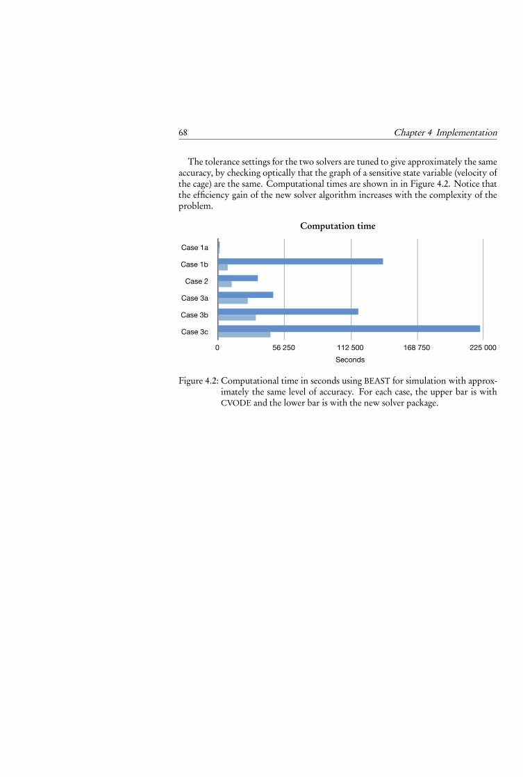
68 Chapter 4 Implementation
The tolerance settings for the two solvers are tuned to give approximately the sameaccuracy, by checking optically that the graph of a sensitive state variable (velocity ofthe cage) are the same. Computational times are shown in in Figure 4.2. Notice thatthe efficiency gain of the new solver algorithm increases with the complexity of theproblem.
Computation time
Case 1a
Case 1b
Case 2
Case 3a
Case 3b
Case 3c
0 56�250 112�500 168�750 225�000
Seconds
Figure 4.2: Computational time in seconds using BEAST for simulation with approx-imately the same level of accuracy. For each case, the upper bar is withCVODE and the lower bar is with the new solver package.
Chapter 5
Conclusions
Not every end is the goal. The end of a melody is not its goal,and yet if a melody has not reached its end, it has not reached itsgoal. A parable.
(Friedrich Nietzsche)
The work in this thesis is concerned with the construction and analysis of efficient nu-merical integration methods for mechanical problems. In particular, for mechanicalmultibody problems with complex force laws describing impact and contact betweenbodies, with application to rolling bearing simulation. The objective of the researchis to develop methods that are more efficient and/or more accurate than generic inte-gration algorithms designed for first order ODEs. Motivation for this research comesdirectly from an industrial need at SKF.
Structure preserving integration algorithms are known to be superior in severalfields of application because of their “physically more correct” behaviour in the nu-merical solution. For example, correct (or “almost correct”) energy behaviour. Clas-sically, these types of integrators have been used in celestial mechanics, moleculardynamics, and theoretical physics. A particular hypothesis in our work is that ge-ometric integration algorithms also are favourable for engineering problems such asrotor dynamics and rolling bearing simulations, where they not yet have been usedmuch. This is verified by several simple test examples and by industrial simulationsusing the BEAST software environment.
Mainly two different routes towards more efficient geometric integrators for theproblem class under study have been followed:
1. To use adaptive time stepping. That is, to use so called adaptive geometric in-tegrators. The construction of such integrators is non-trivial, because standardadaptive techniques cannot be used. Indeed, adaptive geometric integration istoday a very active research area, with many open questions. Our contribu-tions to the field are in Paper II, Paper III and Paper IV.
2. To exploit the special structure of the multibody systems of interest in order topin-point expensive and inexpensive computations. In Paper V such an analysis
69
70 Chapter 5 Conclusions
is carried out, and an efficient method gaining from the specific structure issuggested.
We continue with specific conclusions for each of the three papers.
Paper I An analysis of the geometric structure of non-autonomous mechanical prob-lems is carried out, and geometric numerical methods based on this analysisare tested on classical rotor dynamical problems. The geometric integratorsare superior to standard integrators. The paper motivates the use of geometricintegrators for engineering problems.
Paper II We show how to construct adaptive integrators within the framework ofvariational integrators. Further, a time scaling function specifically designedfor multibody problems with contacts is suggested.
Numerical examples show that, in comparison with an adaptive BDF method,the proposed integrator is more accurate at equal computational cost. Also,since the proposed integrator is based on variational principles, its energy be-haviour is correct, contrary to the energy behaviour of the BDF method.
Paper III Based on a vector field splitting technique in conjunction with Sundmantransformation, a new approach for constructing explicit, adaptive, symplecticintegrators for separable Hamiltonian systems is presented.
Comparison with explicit, adaptive, reversible integration is carried out forseveral examples. The examples show that symplecticity and reversibility ispreferable over mere reversibility for many types of problems. In particular,for non-reversible problem.
Paper IV A new approach for adaptive geometric integration is obtained by studyingtime transformation of Nambu–Poisson systems. The approach is based onextension of the phase space, where the additional variable controls the time-stretching rate. The application in mind is adaptive numerical integration bysplitting of Nambu–Poisson Hamiltonians. As an example, a novel integrationmethod for the rigid body problem is presented and analysed.
Paper V A new numerical integrator specifically designed for the problem class understudy (multibody problems with contact forces between bodies) is suggested.Contrary to standard methods for such problems, the proposed integrator re-quires only one evaluation of the contact forces per time step, and no contactJacobians.
Consistency and stability analysis of the proposed integrator is carried out.
Numerical examples show that the proposed integrator is more efficient (interms of number of contact force evaluations) in comparison with standardimplicit integrators.

71
In addition, a numerical solver library for multibody problems has been imple-mented in C++. The object oriented design of the library makes it easy to implementadaptive numerical integration algorithms that exploits the special structure of multi-body systems. In particular, an adaptive geometric integrator has been implementedin this library. Numerical results for an industrial problems in BEAST show that thenew algorithm is more efficient (at the same accuracy level) than a commonly usedstate-of-the-art generic ODE–solver.

72 Chapter 5 Conclusions
Bibliography
[1] R. Abraham and J. E. Marsden. Foundations of mechanics. Benjamin/CummingsPublishing Co. Inc. Advanced Book Program, Reading, Mass., 1978. Secondedition, revised and enlarged, With the assistance of Tudor Ratiu and RichardCushman.
[2] R. Abraham, J. E. Marsden, and T. Ratiu. Manifolds, tensor analysis, and applica-tions, volume 75 of Applied Mathematical Sciences. Springer-Verlag, New York,second edition, 1988.
[3] D. Alekseevsky and P. Guha. On decomposability of Nambu-Poisson tensor.Acta Math. Univ. Comenian. (N.S.), 65(1):1–9, 1996.
[4] V. I. Arnold. Sur la géométrie différentielle des groupes de Lie de dimensioninfinie et ses applications à l’hydrodynamique des fluides parfaits. Ann. Inst.Fourier (Grenoble), 16(fasc. 1):319–361, 1966.
[5] V. I. Arnold. Mathematical methods of classical mechanics, volume 60 of Grad-uate Texts in Mathematics. Springer-Verlag, New York, second edition, 1989.Translated from the Russian by K. Vogtmann and A. Weinstein.
[6] V. I. Arnold. Ordinary differential equations. Universitext. Springer-Verlag,Berlin, 2006. Translated from the Russian by Roger Cooke, Second printing ofthe 1992 edition.
[7] G. Benettin and A. Giorgilli. On the Hamiltonian interpolation of near-to-the-identity symplectic mappings with application to symplectic integration algo-rithms. J. Statist. Phys., 74(5-6):1117–1143, 1994.
[8] S. Blanes and C. J. Budd. Adaptive geometric integrators for Hamiltonian prob-lems with approximate scale invariance. SIAM J. Sci. Comput., 26(4):1089–1113(electronic), 2005.
[9] S. D. Bond and B. J. Leimkuhler. Time-transformations for reversible variablestepsize integration. Numer. Algorithms, 19(1-4):55–71, 1998. Differential alge-braic equations (Grenoble, 1997).
[10] M. P. Calvo and J. M. Sanz-Serna. Variable steps for symplectic integrators. InNumerical analysis 1991 (Dundee, 1991), volume 260 of Pitman Res. Notes Math.Ser., pages 34–48. Longman Sci. Tech., Harlow, 1992.
73
74 Bibliography
[11] R. Chatterjee and L. Takhtajan. Aspects of classical and quantum Nambu me-chanics. Lett. Math. Phys., 37(4):475–482, 1996.
[12] S. Cirilli, E. Hairer, and B. Leimkuhler. Asymptotic error analysis of the adap-tive Verlet method. BIT, 39(1):25–33, 1999.
[13] G. Dahlquist. Stability and error bounds in the numerical integration of ordi-nary differential equations. Inaugural dissertation, University of Stockholm,Almqvist & Wiksells Boktryckeri AB, Uppsala, 1958.
[14] G. G. Dahlquist. A special stability problem for linear multistep methods.Nordisk Tidskr. Informations-Behandling, 3:27–43, 1963.
[15] E. Eich. Convergence results for a coordinate projection method applied to me-chanical systems with algebraic constraints. SIAM J. Numer. Anal., 30(5):1467–1482, 1993.
[16] E. Eich-Soellner and C. Führer. Numerical methods in multibody dynamics.European Consortium for Mathematics in Industry. B. G. Teubner, Stuttgart,1998.
[17] P. Gautheron. Some remarks concerning Nambu mechanics. Lett. Math. Phys.,37(1):103–116, 1996.
[18] B. Gladman, M. Duncan, and J. Candy. Symplectic integrators for long-term in-tegrations in celestial mechanics. Celestial Mech. Dynam. Astronom., 52(3):221–240, 1991.
[19] I. GmbH. SIMPACK Multibody Simulation Software. www.simpack.com.
[20] E. Hairer. Backward analysis of numerical integrators and symplectic methods.Ann. Numer. Math., 1(1-4):107–132, 1994. Scientific computation and differen-tial equations (Auckland, 1993).
[21] E. Hairer. Variable time step integration with symplectic methods. Appl. Nu-mer. Math., 25(2-3):219–227, 1997. Special issue on time integration (Amster-dam, 1996).
[22] E. Hairer and C. Lubich. The life-span of backward error analysis for numericalintegrators. Numer. Math., 76(4):441–462, 1997.
[23] E. Hairer, C. Lubich, and G. Wanner. Geometric numerical integration illus-trated by the störmer/verlet method. Acta Numer., pages 1–51, 2003.
Bibliography 75
[24] E. Hairer, C. Lubich, and G. Wanner. Geometric numerical integration, vol-ume 31 of Springer Series in Computational Mathematics. Springer-Verlag, Berlin,second edition, 2006. Structure-preserving algorithms for ordinary differentialequations.
[25] E. Hairer, S. P. Nørsett, and G. Wanner. Solving ordinary differential equations.I, volume 8 of Springer Series in Computational Mathematics. Springer-Verlag,Berlin, 1987. Nonstiff problems.
[26] E. Hairer and G. Söderlind. Explicit, time reversible, adaptive step size control.SIAM J. Sci. Comput., 26(6):1838–1851 (electronic), 2005.
[27] A. C. Hindmarsh, P. N. Brown, K. E. Grant, S. L. Lee, R. Serban, D. E. Shu-maker, and C. S. Woodward. SUNDIALS: suite of nonlinear and differential/al-gebraic equation solvers. ACM Trans. Math. Software, 31(3):363–396, 2005.
[28] T. Holder, B. Leimkuhler, and S. Reich. Explicit variable step-size and time-reversible integration. Appl. Numer. Math., 39(3-4):367–377, 2001. Special issue:Themes in geometric integration.
[29] W. Huang and B. Leimkuhler. The adaptive Verlet method. SIAM J. Sci. Com-put., 18(1):239–256, 1997. Dedicated to C. William Gear on the occasion of his60th birthday.
[30] L. Hörmander. Riemannian geometry. Lecturenotes, sold at Department of Mathematics, Lund,www.maths.lth.se/publications/Pure-Lecture-Notes.html, 1990.
[31] R. Ibáñez, M. de León, J. C. Marrero, and D. Martin de Diego. Dynamics ofgeneralized Poisson and Nambu-Poisson brackets. J. Math. Phys., 38(5):2332–2344, 1997.
[32] A. Iserles, H. Z. Munthe-Kaas, S. P. Nørsett, and A. Zanna. Lie-group methods.In Acta numerica, 2000, volume 9 of Acta Numer., pages 215–365. CambridgeUniv. Press, Cambridge, 2000.
[33] C. Kane, J. E. Marsden, M. Ortiz, and M. West. Variational integrators andthe Newmark algorithm for conservative and dissipative mechanical systems.Internat. J. Numer. Methods Engrg., 49(10):1295–1325, 2000.
[34] B. Khesin. Topological fluid dynamics. Notices Amer. Math. Soc., 52(1):9–19,2005.
[35] S. Leyendecker. Mechanical integrators for constrained dynamical systems in flex-ible multibody dynamics. phdthesis, University of Kaiserslautern, 2006. PhDthesis.
76 Bibliography
[36] G. Marmo, G. Vilasi, and A. M. Vinogradov. The local structure of n-Poissonand n-Jacobi manifolds. J. Geom. Phys., 25(1-2):141–182, 1998.
[37] J. E. Marsden. Lectures on mechanics, volume 174 of London Mathematical Soci-ety Lecture Note Series. Cambridge University Press, Cambridge, 1992.
[38] J. E. Marsden and T. S. Ratiu. Introduction to mechanics and symmetry, vol-ume 17 of Texts in Applied Mathematics. Springer-Verlag, New York, secondedition, 1999. A basic exposition of classical mechanical systems.
[39] J. E. Marsden and M. West. Discrete mechanics and variational integrators. ActaNumer., 10:357–514, 2001.
[40] R. I. McLachlan and G. R. W. Quispel. What kinds of dynamics are there?Lie pseudogroups, dynamical systems and geometric integration. Nonlinearity,14(6):1689–1705, 2001.
[41] R. I. McLachlan and G. R. W. Quispel. Splitting methods. Acta Numer., 11:341–434, 2002.
[42] S. Mikkola and P. Wiegert. Regularizing time transformations in symplecticand composite integration. Celestial Mech. Dynam. Astronom., 82(4):375–390,2002.
[43] N. Nakanishi. On Nambu-Poisson manifolds. Rev. Math. Phys., 10(4):499–510,1998.
[44] M. Preto and S. Tremaine. A class of symplectic integrators with adaptivetimestep for separable hamiltonian systems. Astron. J., 118(5):2532–2541, 1999.
[45] S. Reich. Backward error analysis for numerical integrators. SIAM J. Numer.Anal., 36(5):1549–1570 (electronic), 1999.
[46] R. Schmid. Infinite dimensional Lie groups with applications to mathematicalphysics. J. Geom. Symmetry Phys., 1:54–120, 2004.
[47] M. Software. ADAMS Multibody Simulation Software. www.mscsoftware.com.
[48] L.-E. Stacke and D. Fritzson. Dynamical behaviour of rolling bearings: simula-tions and experiments. Proc. Instn. Mech. Engrs., 215:499–508, 2001.
[49] D. Stoffer. Variable steps for reversible integration methods. Computing,55(1):1–22, 1995.
[50] J. Struckmeier. Hamiltonian dynamics on the symplectic extended phase spacefor autonomous and non-autonomous systems. J. Phys. A, 38(6):1257–1278,2005.

Bibliography 77
[51] L. Takhtajan. On foundation of the generalized Nambu mechanics. Comm.Math. Phys., 160(2):295–315, 1994.
[52] K. Zare and V. Szebehely. Time transformations in the extended phase-space.Celestial Mech., 11:469–482, 1975.
[53] G. Zhong and J. E. Marsden. Lie-Poisson Hamilton-Jacobi theory and Lie-Poisson integrators. Phys. Lett. A, 133(3):134–139, 1988.


Paper I
Klas Modin.Not yet submitted, 2009.

Geometric Integration of Non-autonomous Systemswith Application to Rotor Dynamics
Klas MODIN a,b
a SKF Engineering & Research CentreMDC, RKs–2, SE–415 50 Göteborg, Sweden
b Centre for Mathematical Sciences, Lund UniversityBox 118, SE–221 00 Lund, SwedenE–mail: [email protected]
March 25, 2009
AbstractGeometric integration of non-autonomous classical engineering problems, such as rotor dy-
namics, is investigated. It is shown, both numerically and by backward error analysis, that ge-ometric (structure preserving) integration algorithms are superior to conventional Runge–Kuttamethods.
Key-words: Geometric numerical integration, splitting methods, rotor dynamics
1 Introduction
In this paper we study geometric numerical integration algorithms for non-autonomous systems. Byclassifying the appropriate Lie sub-algebra of vector fields, the standard framework for backward erroranalysis can be used to explain the superior qualitative behaviour of geometric methods based on thesplitting approach.
The current section continues with a brief review of the general framework for geometric meth-ods, mainly following the approach by Reich [2]. In Section 2 we study geometric integration of linearsystems with non-constant periodic coefficients. A numerical example from classical rotor dynamicsis given. Conclusions are given in Section 3.
We adopt the following notation. P denotes a phase space manifold of dimension n, with localcoordinates x = (x1, . . . , xn). In the case when P is a linear space we also use P. Further, X(P)denotes the linear space of vector fields on P . The flow of X ∈ X(P) is denoted ϕ t
X , where t isthe time parameter. The Lie derivative along X is denoted LX . If X ,Y ∈ X(P) then the vector fieldcommutator [X ,Y ]X = LX Y supplies X(P) with an infinite dimensional Lie algebra structure. Itscorresponding Lie group is the set Diff(P) of diffeomorphisms on P , with composition as groupoperation. (See McLachlan and Quispel [1] and Schmid [3] for issues concerning infinite dimensionalLie groups.)
As usual, the general linear group of n × n–matrices is denoted GL(n) and its corresponding Liealgebra gl(n). We use [A,B]gl for the matrix commutator AB −BA.
If V is a metric linear space, then the linear space of smooth periodic functions �→ V with period2π/Ω is denoted CΩ(V). Notice that this space is closed under differentiation, i.e., if f ∈ CΩ(V) then italso holds that f ′ ∈ CΩ(V).
1
1.1 Geometric Integration and Backward Error Analysis
Let XS (P) be a sub-algebra of X(P), i.e., a linear sub-space which is closed under the commutator.Its corresponding sub-group of Diff(P) is denoted DiffS (P). Let X ∈XS (P) be a vector field whichis to be integrated numerically. Assume that X can be splitted as a sum of explicitly integrable vectorfield also belonging to XS (P). That is, X = Y +Z where Y,Z ∈XS (P) and ϕ t
Y ,ϕ tZ can be computed
explicitly. By various compositions, various numerical integration schemes for ϕ tX are obtained. The
most classical example is Φh = ϕh/2Y ◦ϕh
Z◦ϕh/2
Y , which yields a second order symmetric method (h isthe step-size parameter of the method). Since ϕ t
Y ,ϕ tZ ∈ DiffS (P), and since DiffS (P) is closed un-
der composition (since it is the group operation), it holds that Φh ∈ DiffS (P). Thus, the splittingapproach yields structure preserving methods, which is a key property.
Backward error analysis for structure preserving integrators deals with the question of finding amodified vector field X ∈ XS (P) such that Φh = ϕ
hX
. In conjunction with perturbation theory, suchan analysis can be used to study the dynamical properties of Φh . For splitting methods, backwarderror analysis is particularly simple as the modified vector field, at least formally, is obtained from theBaker–Campbell–Hausdorff (BCH) formula. For details on this framework we refer to Reich [2].
2 Linear Systems
In this section we study non-autonomous systems on a linear phase space P with global coordinatesx = (x1, . . . , xn). More precisely, let G be a Lie sub-group of GL(n) and g its corresponding Lie sub-algebra. We consider systems of the form
x =A(t )x + f (t ) (1)
where A∈ CΩ(g) and f ∈ CΩ(P) is a smooth vector valued periodic function with period T = 2π/Ω.Our objective is to construct geometric integrators for (1). Of course, since the system is linear, thereis a closed form formula for its solution. However, in engineering applications, e.g. finite elementanalysis, the system is typically very large so computing the exponential matrix, which is necessaryfor the exact solution, is not computationally efficient. Also, it might not be possible to analyticallyintegrate f and A over t , which is necessary for the exact solution.
In order to study dynamical systems of the form (1) in the framework of geometric integration, weneed, first of all, to extend the phase space to P= P×� to include the time variable in the dynamics.Coordinates on P are now given by (x , t ) and the new independent variable is denoted τ (in practicewe always have t (τ) = τ). Further, we need to find a Lie sub-algebra of X(P) which captures theform (1). For this purpose, consider the set of vector field on P given by
LΩ(P,g) =�
X ∈X(P) X (x , t ) = (A(t )x + f (t ),α), A∈ CΩ(g), f ∈ CΩ(P), α ∈�
�. (2)
We now continue with some results concerning properties of LΩ(P,g). The first result states thatit actually is a Lie sub-algebra.
Proposition 2.1. The set of vector fields LΩ(P,g) is a Lie sub-algebra of X(P).
Proof. We need to check that LΩ(P,g) is closed under vector operations and under the Lie bracket.That is, X ,Y ∈LΩ(P,g) should imply aX + bY ∈LΩ(P,g) for a, b ∈� and [X ,Y ]X ∈LΩ(P,g).
With X (x , t ) = (A(t )x + f (t ),α) and Y (x , t ) = (B(t )x + g (t ),β) we get (aX + bY )(x , t ) =
2
((aA+ bB)(t )x + (a f + b g )(t ),aα+ bβ) which is of the desired form. Further,
[X ,Y ]X =�
A(t ) A′(t )x + f ′(t )0 0
��B(t )x + g (t )
β
�−�
B(t ) B ′(t )x + g ′(t )0 0
��Ax + f (t )α
�
=�(A(t )B(t )−B(t )A(t )+βA′(t )−αB ′(t ))x +A(t )g (t )−B(t ) f (t )+β f ′(t )−αg ′(t )
0
�
which is of the desired form since AB − BA+βA′ −αB ′ = [A,B]GL+βA′+αB ′ ∈ CΩ(g) and (Ag −B f +β f ′ −αg ′) ∈ CΩ(P).
From the proof above we immediately obtain the following corollary.
Corollary 2.1. The set lΩ = CΩ(g)×CΩ(P)×� equipped with the induced vector operation
a(A, f ,α)+ b (B , g ,β) = (aA+ bB ,a f + b g ,aα+ bβ), a, b ∈�and with the bracket operation
[(A, f ,α), (B , g ,β)]L = ([A,B]GL+βA′+αB ′,Ag −B f +β f ′ −αg ′, 0)
is a Lie algebra which is isomorphic to LΩ(P,g)with isomorphism lΩ � (A, f ,α) �→ (Ax+ f ,α) ∈LΩ(P,g).
Since CΩ(P) and CΩ(g) are infinite dimensional it follows that lΩ, and therefore also LΩ(P,g), isinfinite dimensional. However, a finite dimensional sub-space of CΩ(P) is given by
CΩ,k (P) =�
f ∈ CΩ(P) f (t ) = a0+
k∑i=1
a i cos(iΩt )+ b i sin(iΩt ), a i , b i ∈ P�
(3)
which is the sub-space of CΩ(P) with angular frequencies bounded by kΩ. Notice that the dimensionof CΩ,k (P) is (2k + 1)n and that CΩ,∞(P) = CΩ(P) and CΩ,0(P) = P. Further, CΩ,k (P) is closed underdifferentiation. Clearly, these results also holds for the corresponding sub-space CΩ,l (g) of CΩ(g),except that the dimension is given by (2l + 1)dimg instead.
By replacing CΩ(P) with CΩ,k (P) and CΩ(g) with CΩ,l (g) we get the sub-spaces lΩ,k ,l = CΩ,l (g)×CΩ,m(P)×� of lΩ. In general lΩ,k ,l is not a sub-algebra, due to the fact that A,B ∈ CΩ,l (g) does not ingeneral imply AB ∈ CΩ,l (g). However, in some special cases the implication holds true.
Proposition 2.2. The sub-spaces lΩ,k ,0 = g× CΩ,k (P)×� and lΩ,k ,∞ = CΩ(g)× CΩ,k (P)×� are Liesub-algebras of lΩ. Further, lΩ,k ,0 is finite dimensional with dimension dimg+ (2k + 1)n+ 1.
Clearly, lΩ,k ,0 and lΩ,k ,∞ induces corresponding Lie sub-algebras LΩ,k ,0(P,g) and LΩ,k ,∞(P,g) of LΩ(P,g).
2.1 Geometric Integration
In this section we describe an approach for geometric integration of of systems of the form (1). Theapproach is based on splitting. To this extent we write (1) as an extended system
d
dτ
�xt
�=�
A(t )x + f (t )1
�≡X (x , t ) . (4)
It is clear that X ∈ LΩ(P,g). Since LΩ(P,g) is a Lie sub-algebra of X(P) it corresponds to a Lie sub-group DiffΩ of Diff(P). Geometric integration of (4) now means to find a one-step integration algo-rithm Φh ∈ DiffΩ. There are of several ways to obtain such integrators. One of the simplest, but yetmost powerful ways, is to use a splitting approach. That is, to split the vector field X as a sum of twovector fields each of them of the form (4).
3
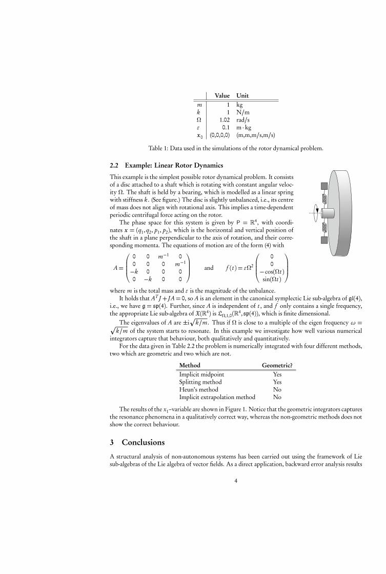
Value Unitm 1 kgk 1 N/mΩ 1.02 rad/sε 0.1 m ·kgx0 (0,0,0,0) (m,m,m/s,m/s)
Table 1: Data used in the simulations of the rotor dynamical problem.
2.2 Example: Linear Rotor Dynamics
This example is the simplest possible rotor dynamical problem. It consistsof a disc attached to a shaft which is rotating with constant angular veloc-ity Ω. The shaft is held by a bearing, which is modelled as a linear springwith stiffness k. (See figure.) The disc is slightly unbalanced, i.e., its centreof mass does not align with rotational axis. This implies a time-dependentperiodic centrifugal force acting on the rotor.
The phase space for this system is given by P = �4, with coordi-nates x = (q1, q2, p1, p2), which is the horizontal and vertical position ofthe shaft in a plane perpendicular to the axis of rotation, and their corre-sponding momenta. The equations of motion are of the form (4) with
A=
⎛⎜⎜⎜⎝0 0 m−1 00 0 0 m−1
−k 0 0 00 −k 0 0
⎞⎟⎟⎟⎠ and f (t ) = εΩ2
⎛⎜⎜⎜⎝00
−cos(Ωt )sin(Ωt )
⎞⎟⎟⎟⎠where m is the total mass and ε is the magnitude of the unbalance.
It holds that AT J + J A= 0, so A is an element in the canonical symplectic Lie sub-algebra of gl(4),i.e., we have g = sp(4). Further, since A is independent of t , and f only contains a single frequency,the appropriate Lie sub-algebra of X(�4) is LΩ,1,0(�4,sp(4)), which is finite dimensional.
The eigenvalues of A are ±i
k/m. Thus if Ω is close to a multiple of the eigen frequency ω =k/m of the system starts to resonate. In this example we investigate how well various numerical
integrators capture that behaviour, both qualitatively and quantitatively.For the data given in Table 2.2 the problem is numerically integrated with four different methods,
two which are geometric and two which are not.
Method Geometric?Implicit midpoint YesSplitting method YesHeun’s method NoImplicit extrapolation method No
The results of the x1–variable are shown in Figure 1. Notice that the geometric integrators capturesthe resonance phenomena in a qualitatively correct way, whereas the non-geometric methods does notshow the correct behaviour.
3 Conclusions
A structural analysis of non-autonomous systems has been carried out using the framework of Liesub-algebras of the Lie algebra of vector fields. As a direct application, backward error analysis results
4

0 200 400 600 800 1000�6
�3
0
3
6
0 200 400 600 800 1000�6
�3
0
3
6
0 200 400 600 800 1000�6
�3
0
3
6
0 200 400 600 800 1000�6
�3
0
3
6
0 200 400 600 800 1000�6
�3
0
3
6
Time t
Figure 1: Results for q1 variable for the simple linear rotor example. From top: (1) exact solu-tion, (2) implicit midpoint, geometric, (3) Störmer–Verlet, geometric, (4) implicit Runge–Kutta, non-geometric, (5) explicit Runge-Kutta, non-geometric. All methods are second order accurate. Noticethe superior qualitative and quantitative behaviour of the geometric methods.
5
are obtained for this class of problems. Numerical examples of a classical rotor dynamical problemshow that the geometric methods preserving the structure of the problem indeed are favourable overnon-geometric dito.
Acknowledgement The author is grateful to Dag Fritzson, Claus Führer and Gustaf Söderlind forhelpful discussions. The author would also like to thank SKF for the support given.
References
[1] R. I. McLachlan and G. R. W. Quispel. What kinds of dynamics are there? Lie pseudogroups,dynamical systems and geometric integration. Nonlinearity, 14(6):1689–1705, 2001.
[2] S. Reich. Backward error analysis for numerical integrators. SIAM J. Numer. Anal., 36(5):1549–1570 (electronic), 1999.
[3] R. Schmid. Infinite dimensional Lie groups with applications to mathematical physics. J. Geom.Symmetry Phys., 1:54–120, 2004.
6

Paper II
Klas Modin and Claus Führer.ZAMM Z. Angew. Math. Mech., 86(10):785–794, 2006.

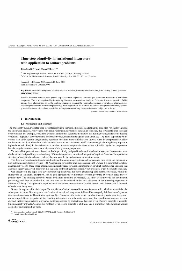
ZAMM · Z. Angew. Math. Mech. 86, No. 10, 785 – 794 (2006) / DOI 10.1002/zamm.200610286
Time-step adaptivity in variational integratorswith application to contact problems
Klas Modin1,∗ and Claus Fuhrer2,∗∗
1 SKF Engineering Research Centre, MDC RKs–2, 415 50 Goteborg, Sweden2 Centre for Mathematical Sciences, Lund University, Box 118, 221 00 Lund, Sweden
Received 15 February 2006, accepted 8 June 2006Published online 9 October 2006
Key words variational integrators, variable step-size methods, Poincare transformations, time scaling, contact problemsMSC (2000) 37M15
Variable time-step methods, with general step-size control objectives, are developed within the framework of variationalintegrators. This is accomplished by introducing discrete transformations similar to Poincares time transformation. Whilegaining from adaptive time-steps, the resulting integrators preserve the structural advantages of variational integrators, i. e.,they are symplectic and momentum preserving. As an application, the methods are utilized for dynamic multibody systemsgoverned by contact force laws. A suitable scaling function defining the step-size control objective is derived.
c© 2006 WILEY-VCH Verlag GmbH & Co. KGaA, Weinheim
1 Introduction
1.1 Motivation and overview
The philosophy behind variable time-step integrators is to increase efficiency by adapting the time-step “on the fly”, duringthe integration process. For systems with heavily alternating dynamics, the gain in efficiency due to variable time-steps canbe substantial. For example, consider a dynamic system that describes the motion of a rolling bearing under some loadingconditions. Typically, the components frequently bounce, roll and slide against each other, see [13]. Thus, depending on thecurrent state of the system, the governing equations vary from a non-stiff character (typical when the components are eithernot in contact at all, or when there is slow motion in the active contacts) to a stiff character (typical during heavy impacts athigh relative velocities). In these situations a variable time-step integrator is favourable as it, ideally, regularizes the problemby adapting the time-step to the local character of the governing equations.
Variational integrators form a class of methods specifically designed for dynamic mechanical systems. In contrast to stan-dard methods designed for general ordinary differential equations, variational integrators “replicate” much of the qualitativestructure of analytical mechanics. Indeed, they are symplectic and preserve momentum maps.
The theory of variational integrators is developed for autonomous systems and for constant time-steps. An extension tonon-autonomous systems is given in [12]. An extension to variable time-steps is given in [8], where it is shown that by takingan extended velocity phase space approach one naturally leads to variational integrators in which the time-step varies so thatenergy is exactly conserved. However, this step-size control objective is generally not preferable when it comes to efficiency.
Our objective in the paper is to develop time-step adaptivity, for more general step-size control objectives, within theframework of variational integrators, and to give applications to multibody systems governed by contact force laws ofpenalty type. The resulting methods benefit both from structural advantages, i. e., they are symplectic and momentumpreserving, and from adaptivity, i. e., the time-step can be adapted to the local character of the governing equations toincrease efficiency. Throughout the paper we restrict ourselves to autonomous systems in order to fit the standard frameworkof variational integrators.
Next to the organization of the paper. The remainder of this section outlines some known results, which are essential to thesubsequent sections. First we give a brief review of variational integrators, followed by an equally brief review of dynamictime transformations for Hamiltonian systems. Sect. 2 contains the main result: variable time-step variational integratorsare developed. Some properties of the resulting integrators, and relation to integrators for Hamiltonian systems, are alsoderived. In Sect. 3 applications to dynamic systems governed by contact force laws are given. The first example is a simple,but numerically intricate, “contact test problem”. The second example is a billiard, i. e., a multiple of balls bouncing againsteach other and surrounding walls.
∗ Corresponding author, e-mail: [email protected], Phone: +46 31 337 3276∗∗ e-mail: [email protected]
c© 2006 WILEY-VCH Verlag GmbH & Co. KGaA, Weinheim
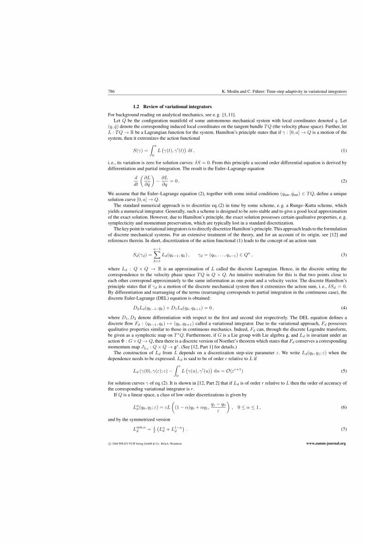
786 K. Modin and C. Fuhrer: Time-step adaptivity in variational integrators
1.2 Review of variational integrators
For background reading on analytical mechanics, see e. g. [1,11].Let Q be the configuration manifold of some autonomous mechanical system with local coordinates denoted q. Let
(q, q) denote the corresponding induced local coordinates on the tangent bundle TQ (the velocity phase space). Further, letL : TQ → R be a Lagrangian function for the system. Hamilton’s principle states that if γ : [0, a] → Q is a motion of thesystem, then it extremizes the action functional
S(γ) =∫ a
0L
(γ(t), γ′(t)
)dt , (1)
i. e., its variation is zero for solution curves: δS = 0. From this principle a second order differential equation is derived bydifferentiation and partial integration. The result is the Euler–Lagrange equation
d
dt
(∂L
∂q
)− ∂L
∂q= 0 . (2)
We assume that the Euler–Lagrange equation (2), together with some initial conditions (qinit, qinit) ∈ TQ, define a uniquesolution curve [0, a] → Q.
The standard numerical approach is to discretize eq. (2) in time by some scheme, e. g. a Runge–Kutta scheme, whichyields a numerical integrator. Generally, such a scheme is designed to be zero stable and to give a good local approximationof the exact solution. However, due to Hamilton’s principle, the exact solution possesses certain qualitative properties, e. g.symplecticity and momentum preservation, which are typically lost in a standard discretization.
The key point in variational integrators is to directly discretize Hamilton’s principle. This approach leads to the formulationof discrete mechanical systems. For an extensive treatment of the theory, and for an account of its origin, see [12] andreferences therein. In short, discretization of the action functional (1) leads to the concept of an action sum
Sd(γd) =n−1∑k=1
Ld(qk−1, qk) , γd = (q0, . . . , qn−1) ∈ Qn , (3)
where Ld : Q × Q → R is an approximation of L called the discrete Lagrangian. Hence, in the discrete setting thecorrespondence to the velocity phase space TQ is Q × Q. An intuitive motivation for this is that two points close toeach other correspond approximately to the same information as one point and a velocity vector. The discrete Hamilton’sprinciple states that if γd is a motion of the discrete mechanical system then it extremizes the action sum, i. e., δSd = 0.By differentiation and rearranging of the terms (rearranging corresponds to partial integration in the continuous case), thediscrete Euler-Lagrange (DEL) equation is obtained:
D2Ld(qk−1, qk) + D1Ld(qk, qk+1) = 0 , (4)
where D1, D2 denote differentiation with respect to the first and second slot respectively. The DEL equation defines adiscrete flow Fd : (qk−1, qk) �→ (qk, qk+1) called a variational integrator. Due to the variational approach, Fd possessesqualitative properties similar to those in continuous mechanics. Indeed, Fd can, through the discrete Legendre transform,be given as a symplectic map on T ∗Q. Furthermore, if G is a Lie group with Lie algebra g, and Ld is invariant under anaction Φ : G×Q → Q, then there is a discrete version of Noether’s theorem which states that Fd conserves a correspondingmomentum map JLd
: Q × Q → g∗. (See [12, Part 1] for details.)The construction of Ld from L depends on a discretization step-size parameter ε. We write Ld(q0, q1; ε) when the
dependence needs to be expressed. Ld is said to be of order r relative to L if
Ld (γ(0), γ(ε); ε) −∫ ε
0L
(γ(u), γ′(u)
)du = O(εr+1) (5)
for solution curves γ of eq. (2). It is shown in [12, Part 2] that if Ld is of order r relative to L then the order of accuracy ofthe corresponding variational integrator is r.
If Q is a linear space, a class of low order discretizations is given by
Lαd (q0, q1; ε) = εL
((1 − α)q0 + αq1,
q1 − q0
ε
), 0 ≤ α ≤ 1 , (6)
and by the symmetrized version
Lsym,αd = 1
2
(Lα
d + L1−αd
). (7)
c© 2006 WILEY-VCH Verlag GmbH & Co. KGaA, Weinheim www.zamm-journal.org
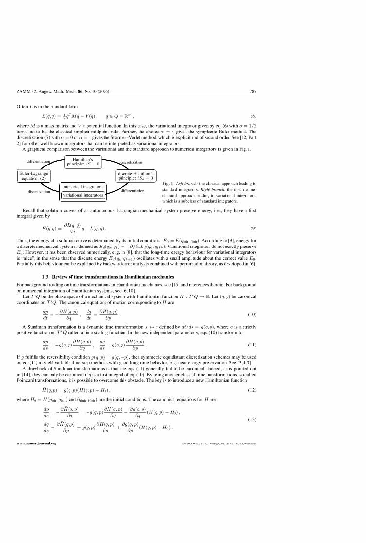
ZAMM · Z. Angew. Math. Mech. 86, No. 10 (2006) 787
Often L is in the standard form
L(q, q) = 12 qT Mq − V (q) , q ∈ Q = R
m , (8)
where M is a mass matrix and V a potential function. In this case, the variational integrator given by eq. (6) with α = 1/2turns out to be the classical implicit midpoint rule. Further, the choice α = 0 gives the symplectic Euler method. Thediscretization (7) with α = 0 or α = 1 gives the Stormer–Verlet method, which is explicit and of second order. See [12, Part2] for other well known integrators that can be interpreted as variational integrators.
A graphical comparison between the variational and the standard approach to numerical integrators is given in Fig. 1.�� ��
�� �
Hamilton’sprinciple: δS = 0differentiation
��discretization
���� ��
�� �
Euler-Lagrangeequation: (2)
�� ��
�� �
discrete Hamilton’sprinciple: δSd = 0
differentiation��
numerical integrators�� ��
�� �variational integrators
� �
�� ��
discretization ��
Fig. 1 Left branch: the classical approach leading tostandard integrators. Right branch: the discrete me-chanical approach leading to variational integrators,which is a subclass of standard integrators.
Recall that solution curves of an autonomous Lagrangian mechanical system preserve energy, i. e., they have a firstintegral given by
E(q, q) =∂L(q, q)
∂qq − L(q, q) . (9)
Thus, the energy of a solution curve is determined by its initial conditions: E0 = E(qinit, qinit). According to [9], energy fora discrete mechanical system is defined as Ed(q0, q1) = −∂/∂εLd(q0, q1; ε). Variational integrators do not exactly preserveEd. However, it has been observed numerically, e. g. in [8], that the long-time energy behaviour for variational integratorsis “nice”, in the sense that the discrete energy Ed(qk, qk+1) oscillates with a small amplitude about the correct value E0.Partially, this behaviour can be explained by backward error analysis combined with perturbation theory, as developed in [6].
1.3 Review of time transformations in Hamiltonian mechanics
For background reading on time transformations in Hamiltonian mechanics, see [15] and references therein. For backgroundon numerical integration of Hamiltonian systems, see [6,10].
Let T ∗Q be the phase space of a mechanical system with Hamiltonian function H : T ∗Q → R. Let (q, p) be canonicalcoordinates on T ∗Q. The canonical equations of motion corresponding to H are
dp
dt= − ∂H(q, p)
∂q,
dq
dt=
∂H(q, p)∂p
. (10)
A Sundman transformation is a dynamic time transformation s ↔ t defined by dt/ds = g(q, p), where g is a strictlypositive function on T ∗Q called a time scaling function. In the new independent parameter s, eqs. (10) transform to
dp
ds= −g(q, p)
∂H(q, p)∂q
,dq
ds= g(q, p)
∂H(q, p)∂p
. (11)
If g fulfills the reversibility condition g(q, p) = g(q, −p), then symmetric equidistant discretization schemes may be usedon eq. (11) to yield variable time-step methods with good long-time behavior, e. g. near energy preservation. See [3,4,7].
A drawback of Sundman transformations is that the eqs. (11) generally fail to be canonical. Indeed, as is pointed outin [14], they can only be canonical if g is a first integral of eq. (10). By using another class of time transformations, so calledPoincare transformations, it is possible to overcome this obstacle. The key is to introduce a new Hamiltonian function
H(q, p) = g(q, p)(H(q, p) − H0) , (12)
where H0 = H(pinit, qinit) and (qinit, pinit) are the initial conditions. The canonical equations for H are
dp
ds= − ∂H(q, p)
∂q= −g(q, p)
∂H(q, p)∂q
− ∂g(q, p)∂q
(H(q, p) − H0) ,
dq
ds=
∂H(q, p)∂p
= g(q, p)∂H(q, p)
∂p+
∂g(q, p)∂p
(H(q, p) − H0) .
(13)
www.zamm-journal.org c© 2006 WILEY-VCH Verlag GmbH & Co. KGaA, Weinheim
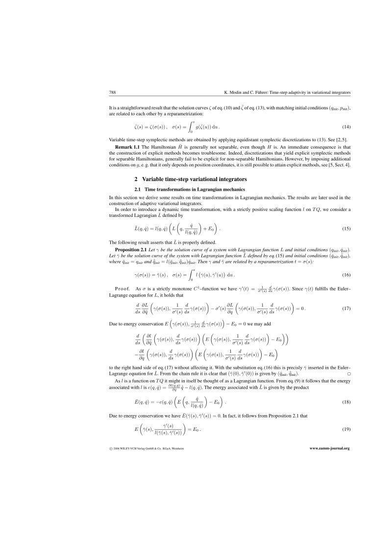
788 K. Modin and C. Fuhrer: Time-step adaptivity in variational integrators
It is a straightforward result that the solution curves ζ of eq. (10) and ζ of eq. (13), with matching initial conditions (qinit, pinit),are related to each other by a reparametrization:
ζ(s) = ζ(σ(s)) , σ(s) =∫ s
0g(ζ(u)) du . (14)
Variable time-step symplectic methods are obtained by applying equidistant symplectic discretizations to (13). See [2,5].
Remark 1.1 The Hamiltonian H is generally not separable, even though H is. An immediate consequence is thatthe construction of explicit methods becomes troublesome. Indeed, discretizations that yield explicit symplectic methodsfor separable Hamiltonians, generally fail to be explicit for non-separable Hamiltonians. However, by imposing additionalconditions on g, e. g. that it only depends on position coordinates, it is still possible to attain explicit methods, see [5, Sect. 4].
2 Variable time-step variational integrators
2.1 Time transformations in Lagrangian mechanics
In this section we derive some results on time transformations in Lagrangian mechanics. The results are later used in theconstruction of adaptive variational integrators.
In order to introduce a dynamic time transformation, with a strictly positive scaling function l on TQ, we consider atransformed Lagrangian L defined by
L(q, q) = l(q, q)(
L
(q,
q
l(q, q)
)+ E0
). (15)
The following result asserts that L is properly defined.
Proposition 2.1 Let γ be the solution curve of a system with Lagrangian function L and initial conditions (qinit, qinit).Let γ be the solution curve of the system with Lagrangian function L defined by eq. (15) and initial conditions (qinit, ˙qinit),where qinit = qinit and ˙qinit = l(qinit, ˙qinit)qinit. Then γ and γ are related by a reparametrization t = σ(s):
γ(σ(s)) = γ(s) , σ(s) =∫ s
0l(γ(u), γ′(u)
)du . (16)
P r o o f. As σ is a strictly monotone C1–function we have γ′(t) = 1σ′(s)
dds γ(σ(s)). Since γ(t) fulfills the Euler–
Lagrange equation for L, it holds that
d
ds
∂L
∂q
(γ(σ(s)),
1σ′(s)
d
dsγ(σ(s))
)− σ′(s)
∂L
∂q
(γ(σ(s)),
1σ′(s)
d
dsγ(σ(s))
)= 0 . (17)
Due to energy conservation E(γ(σ(s)), 1
σ′(s)dds γ(σ(s))
)− E0 = 0 we may add
d
ds
(∂l
∂q
(γ(σ(s)),
d
dsγ(σ(s))
)(E
(γ(σ(s)),
1σ′(s)
d
dsγ(σ(s))
)− E0
))
− ∂l
∂q
(γ(σ(s)),
d
dsγ(σ(s))
)(E
(γ(σ(s)),
1σ′(s)
d
dsγ(σ(s))
)− E0
)
to the right hand side of eq. (17) without affecting it. With the substitution eq. (16) this is precisly γ inserted in the Euler–Lagrange equation for L. From the chain rule it is clear that (γ(0), γ′(0)) is given by (qinit, ˙qinit).
As l is a function on TQ it might in itself be thought of as a Lagrangian function. From eq. (9) it follows that the energyassociated with l is e(q, q) = ∂l(q,q)
∂q q − l(q, q). The energy associated with L is given by the product
E(q, q) = −e(q, q)(
E
(q,
q
l(q, q)
)− E0
). (18)
Due to energy conservation we have E(γ(s), γ′(s)) = 0. In fact, it follows from Proposition 2.1 that
E
(γ(s),
γ′(s)l(γ(s), γ′(s))
)= E0 . (19)
c© 2006 WILEY-VCH Verlag GmbH & Co. KGaA, Weinheim www.zamm-journal.org
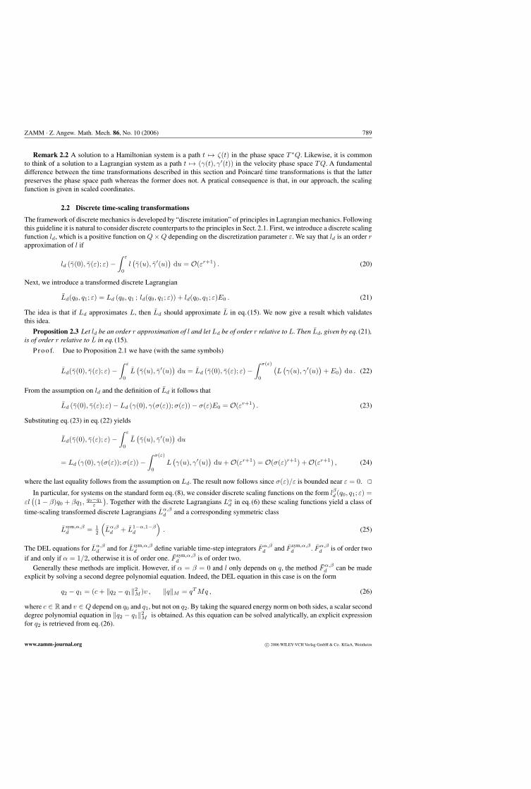
ZAMM · Z. Angew. Math. Mech. 86, No. 10 (2006) 789
Remark 2.2 A solution to a Hamiltonian system is a path t �→ ζ(t) in the phase space T ∗Q. Likewise, it is commonto think of a solution to a Lagrangian system as a path t �→ (γ(t), γ′(t)) in the velocity phase space TQ. A fundamentaldifference between the time transformations described in this section and Poincare time transformations is that the latterpreserves the phase space path whereas the former does not. A pratical consequence is that, in our approach, the scalingfunction is given in scaled coordinates.
2.2 Discrete time-scaling transformations
The framework of discrete mechanics is developed by “discrete imitation” of principles in Lagrangian mechanics. Followingthis guideline it is natural to consider discrete counterparts to the principles in Sect. 2.1. First, we introduce a discrete scalingfunction ld, which is a positive function on Q × Q depending on the discretization parameter ε. We say that ld is an order rapproximation of l if
ld (γ(0), γ(ε); ε) −∫ ε
0l(γ(u), γ′(u)
)du = O(εr+1) . (20)
Next, we introduce a transformed discrete Lagrangian
Ld(q0, q1; ε) = Ld (q0, q1 ; ld(q0, q1; ε)) + ld(q0, q1; ε)E0 . (21)
The idea is that if Ld approximates L, then Ld should approximate L in eq. (15). We now give a result which validatesthis idea.
Proposition 2.3 Let ld be an order r approximation of l and let Ld be of order r relative to L. Then Ld, given by eq. (21),is of order r relative to L in eq. (15).
P r o o f. Due to Proposition 2.1 we have (with the same symbols)
Ld(γ(0), γ(ε); ε) −∫ ε
0L
(γ(u), γ′(u)
)du = Ld (γ(0), γ(ε); ε) −
∫ σ(ε)
0
(L
(γ(u), γ′(u)
)+ E0
)du . (22)
From the assumption on ld and the definition of Ld it follows that
Ld (γ(0), γ(ε); ε) − Ld (γ(0), γ(σ(ε));σ(ε)) − σ(ε)E0 = O(εr+1) . (23)
Substituting eq. (23) in eq. (22) yields
Ld(γ(0), γ(ε); ε) −∫ ε
0L
(γ(u), γ′(u)
)du
= Ld (γ(0), γ(σ(ε));σ(ε)) −∫ σ(ε)
0L
(γ(u), γ′(u)
)du + O(εr+1) = O(σ(ε)r+1) + O(εr+1) , (24)
where the last equality follows from the assumption on Ld. The result now follows since σ(ε)/ε is bounded near ε = 0.
In particular, for systems on the standard form eq. (8), we consider discrete scaling functions on the form lβd (q0, q1; ε) =εl
((1 − β)q0 + βq1,
q0−q1ε
). Together with the discrete Lagrangians Lα
d in eq. (6) these scaling functions yield a class of
time-scaling transformed discrete Lagrangians Lα,βd and a corresponding symmetric class
Lsym,α,βd = 1
2
(Lα,β
d + L1−α,1−βd
). (25)
The DEL equations for Lα,βd and for Lsym,α,β
d define variable time-step integrators Fα,βd and F sym,α,β
d . Fα,βd is of order two
if and only if α = 1/2, otherwise it is of order one. F sym,α,βd is of order two.
Generally these methods are implicit. However, if α = β = 0 and l only depends on q, the method Fα,βd can be made
explicit by solving a second degree polynomial equation. Indeed, the DEL equation in this case is on the form
q2 − q1 = (c + ‖q2 − q1‖2M )v , ‖q‖M = qT Mq , (26)
where c ∈ R and v ∈ Q depend on q0 and q1, but not on q2. By taking the squared energy norm on both sides, a scalar seconddegree polynomial equation in ‖q2 − q1‖2
M is obtained. As this equation can be solved analytically, an explicit expressionfor q2 is retrieved from eq. (26).
www.zamm-journal.org c© 2006 WILEY-VCH Verlag GmbH & Co. KGaA, Weinheim
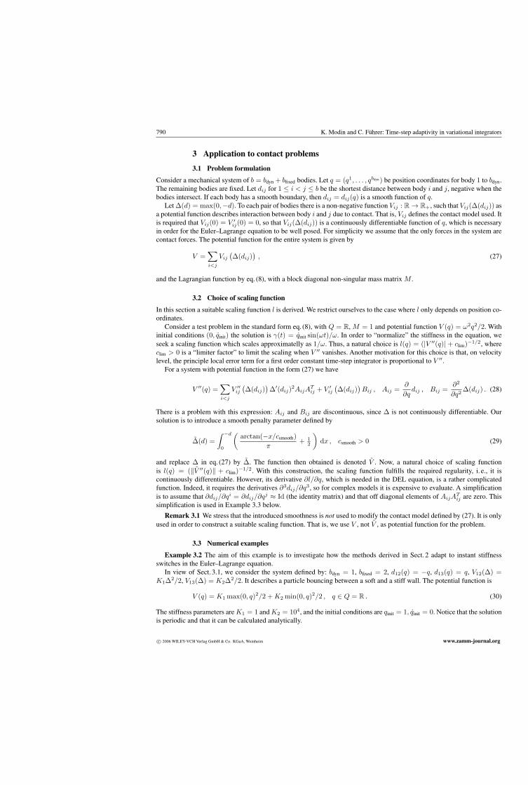
790 K. Modin and C. Fuhrer: Time-step adaptivity in variational integrators
3 Application to contact problems
3.1 Problem formulation
Consider a mechanical system of b = bdyn + bfixed bodies. Let q = (q1, . . . , qbdyn) be position coordinates for body 1 to bdyn.The remaining bodies are fixed. Let dij for 1 ≤ i < j ≤ b be the shortest distance between body i and j, negative when thebodies intersect. If each body has a smooth boundary, then dij = dij(q) is a smooth function of q.
Let Δ(d) = max(0, −d). To each pair of bodies there is a non-negative function Vij : R → R+, such that Vij(Δ(dij)) asa potential function describes interaction between body i and j due to contact. That is, Vij defines the contact model used. Itis required that Vij(0) = V ′
ij(0) = 0, so that Vij(Δ(dij)) is a continuously differentiable function of q, which is necessaryin order for the Euler–Lagrange equation to be well posed. For simplicity we assume that the only forces in the system arecontact forces. The potential function for the entire system is given by
V =∑i<j
Vij
(Δ(dij)
), (27)
and the Lagrangian function by eq. (8), with a block diagonal non-singular mass matrix M .
3.2 Choice of scaling function
In this section a suitable scaling function l is derived. We restrict ourselves to the case where l only depends on position co-ordinates.
Consider a test problem in the standard form eq. (8), with Q = R, M = 1 and potential function V (q) = ω2q2/2. Withinitial conditions (0, qinit) the solution is γ(t) = qinit sin(ωt)/ω. In order to “normalize” the stiffness in the equation, weseek a scaling function which scales approximatelly as 1/ω. Thus, a natural choice is l(q) = (|V ′′(q)| + clim)−1/2, whereclim > 0 is a “limiter factor” to limit the scaling when V ′′ vanishes. Another motivation for this choice is that, on velocitylevel, the principle local error term for a first order constant time-step integrator is proportional to V ′′.
For a system with potential function in the form (27) we have
V ′′(q) =∑i<j
V ′′ij
(Δ(dij)
)Δ′(dij)2AijA
Tij + V ′
ij
(Δ(dij)
)Bij , Aij =
∂
∂qdij , Bij =
∂2
∂q2 Δ(dij) . (28)
There is a problem with this expression: Aij and Bij are discontinuous, since Δ is not continuously differentiable. Oursolution is to introduce a smooth penalty parameter defined by
Δ(d) =∫ −d
0
(arctan(−x/csmooth)
π+ 1
2
)dx , csmooth > 0 (29)
and replace Δ in eq. (27) by Δ. The function then obtained is denoted V . Now, a natural choice of scaling functionis l(q) = (‖V ′′(q)‖ + clim)−1/2. With this construction, the scaling function fulfills the required regularity, i. e., it iscontinuously differentiable. However, its derivative ∂l/∂q, which is needed in the DEL equation, is a rather complicatedfunction. Indeed, it requires the derivatives ∂3dij/∂q3, so for complex models it is expensive to evaluate. A simplificationis to assume that ∂dij/∂qi = ∂dij/∂qj ≈ Id (the identity matrix) and that off diagonal elements of AijA
Tij are zero. This
simplification is used in Example 3.3 below.
Remark 3.1 We stress that the introduced smoothness is not used to modify the contact model defined by (27). It is onlyused in order to construct a suitable scaling function. That is, we use V , not V , as potential function for the problem.
3.3 Numerical examples
Example 3.2 The aim of this example is to investigate how the methods derived in Sect. 2 adapt to instant stiffnessswitches in the Euler–Lagrange equation.
In view of Sect. 3.1, we consider the system defined by: bdyn = 1, bfixed = 2, d12(q) = −q, d13(q) = q, V12(Δ) =K1Δ2/2, V13(Δ) = K2Δ2/2. It describes a particle bouncing between a soft and a stiff wall. The potential function is
V (q) = K1 max(0, q)2/2 + K2 min(0, q)2/2 , q ∈ Q = R . (30)
The stiffness parameters are K1 = 1 and K2 = 104, and the initial conditions are qinit = 1, qinit = 0. Notice that the solutionis periodic and that it can be calculated analytically.
c© 2006 WILEY-VCH Verlag GmbH & Co. KGaA, Weinheim www.zamm-journal.org
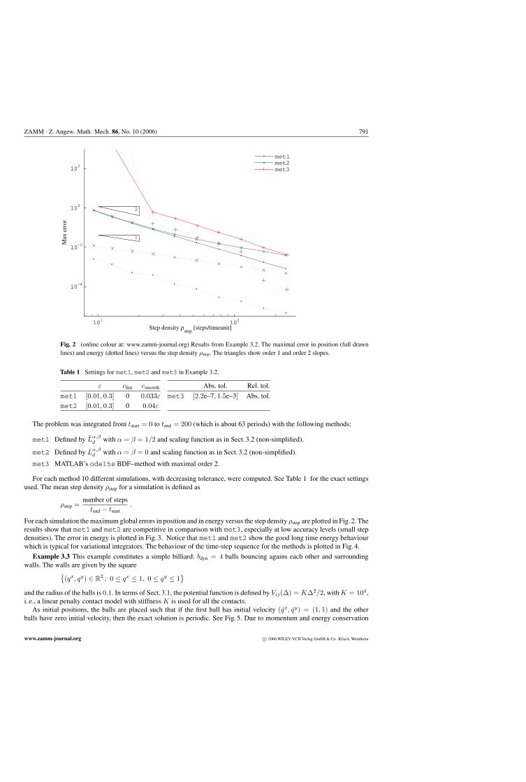
ZAMM · Z. Angew. Math. Mech. 86, No. 10 (2006) 791
101
102
10−4
10−2
100
102
Step density ρstep
[steps/timeunit]
Max
err
or
met1met2met3
1
2
Fig. 2 (online colour at: www.zamm-journal.org) Results from Example 3.2. The maximal error in position (full drawnlines) and energy (dotted lines) versus the step density ρstep. The triangles show order 1 and order 2 slopes.
Table 1 Settings for met1, met2 and met3 in Example 3.2.
ε clim csmooth
met1 [0.01, 0.3] 0 0.033ε
met2 [0.01, 0.3] 0 0.04ε
Abs. tol. Rel. tol.
met3 [2.2e–7, 1.5e–3] Abs. tol.
The problem was integrated from tstart = 0 to tend = 200 (which is about 63 periods) with the following methods:
met1 Defined by Lα,βd with α = β = 1/2 and scaling function as in Sect. 3.2 (non-simplified).
met2 Defined by Lα,βd with α = β = 0 and scaling function as in Sect. 3.2 (non-simplified).
met3 MATLAB’s ode15s BDF–method with maximal order 2.
For each method 10 different simulations, with decreasing tolerance, were computed. See Table 1 for the exact settingsused. The mean step density ρstep for a simulation is defined as
ρstep =number of steps
tend − tstart.
For each simulation the maximum global errors in position and in energy versus the step density ρstep are plotted in Fig. 2. Theresults show that met1 and met2 are competitive in comparison with met3, especially at low accuracy levels (small stepdensities). The error in energy is plotted in Fig. 3. Notice that met1 and met2 show the good long time energy behaviourwhich is typical for variational integrators. The behaviour of the time-step sequence for the methods is plotted in Fig. 4.
Example 3.3 This example constitutes a simple billiard: bdyn = 4 balls bouncing agains each other and surroundingwalls. The walls are given by the square{
(qx, qy) ∈ R2 ; 0 ≤ qx ≤ 1, 0 ≤ qy ≤ 1
}and the radius of the balls is 0.1. In terms of Sect. 3.1, the potential function is defined by Vij(Δ) = KΔ2/2, with K = 104,i. e., a linear penalty contact model with stiffness K is used for all the contacts.
As initial positions, the balls are placed such that if the first ball has initial velocity (qx, qy) = (1, 1) and the otherballs have zero initial velocity, then the exact solution is periodic. See Fig. 5. Due to momentum and energy conservation
www.zamm-journal.org c© 2006 WILEY-VCH Verlag GmbH & Co. KGaA, Weinheim
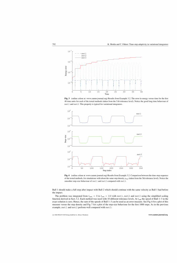
792 K. Modin and C. Fuhrer: Time-step adaptivity in variational integrators
0 5 10 15 20 25 30 35 40
10−4
10−3
10−2
10−1
Time
Ene
rgy
erro
r
met1met2met3
Fig. 3 (online colour at: www.zamm-journal.org) Results from Example 3.2. The error in energy versus time for the first40 time units for each of the tested methods (taken from the 5:th tolerance level). Notice the good long time behaviour ofmet1 and met2. This property is typical for variational integrators.
10−4
10−2
100
10−4
10−2
100
Step
−si
ze
0 50 100 150 200 250 300 35010
−4
10−2
100
Step index
met1
met2
met3
Fig. 4 (online colour at: www.zamm-journal.org) Results from Example 3.2. Comparison between the time-step sequenceof the tested methods, for simulations with about the same step density ρstep (taken from the 5th tolerance level). Notice thesmoother step-size behaviour of met1 and met2 compared with met3.
Ball 1 should make a full stop after impact with Ball 2 which should continue with the same velocity as Ball 1 had beforethe impact.
The problem was integrated from tstart = 0 to tend = 2.0 with met1, met2 and met3 using the simplified scalingfunction derived in Sect. 3.2. Each method was used with 10 different tolerance levels. At tend the speed of Ball 1–3 in theexact solution is zero. Hence, the sum of the speeds of Ball 1–3 can be used as an error measure. See Fig. 6 for a plot of thismeasure versus the step density and Fig. 7 for a plot of the step-size behaviour for the first 1000 steps. As in the previousexample, met1 and met2 perform well compared with met3.
c© 2006 WILEY-VCH Verlag GmbH & Co. KGaA, Weinheim www.zamm-journal.org

ZAMM · Z. Angew. Math. Mech. 86, No. 10 (2006) 793
2
4 3
1
Fig. 5 Setup in Example 3.3. The initialvelocity of Ball 1 is such that the dottedpath is followed in the exact solution.
102
103
10−5
10−4
10−3
10−2
10−1
100
Step density [steps/timeunit]
Spee
d er
ror
for
ball
1−−
3
met1met2met3
Fig. 6 (online colour at: www.zamm-journal.org) Error in speed at tend for Ball 1–3 (fulldrawn lines) and error in energy (dotted lines) versus step density ρstep for each testedmethod.
0 500 1000
10−5
10−4
10−3
10−2
10−1
Step
−si
ze
Step index0 500 1000
Step index
met1 met3
Fig. 7 (online colour at: www.zamm-journal.org) Step-size sequence for the first 1000 steps with met1 and met3 (takenfrom the 10th tolerance level). Notice again that met1 yields a smoother step-size sequence than met3. Also, the “drops”in met3 down to about 10−5, which are likely due to failed steps, do not occur in met1.
4 Conclusions
Variable time-step methods have been developed within the framework of variational integrators. Hence, adaptive integratorswith structural properties suitable for mechanical problems have been obtained. A time scaling function suitable for dynamicmultibody problems governed by contact force laws of penalty type have been developed. Numerical examples with methodsfrom the class given by Lα,β
d have been tested with the derived scaling function. The results show that the methods adaptthe time-step length to contact conditions in a more stable and more efficient way than a standard adaptive BDF method.
Acknowledgements The authors are grateful to Dag Fritzson and Gustaf Soderlind for helpful discussions and comments on the work.
References
[1] V. I. Arnold, Mathematical methods of classical mechanics (Springer-Verlag, New York, 1989).[2] S. Blanes and C. J. Budd, Explicit, adaptive, symplectic (easy) integrators using scale invariant regularisations and canonical
transformations, Celest. Mech. Dyn. Astron. (Netherlands) 89, 383–405 (2004).
www.zamm-journal.org c© 2006 WILEY-VCH Verlag GmbH & Co. KGaA, Weinheim
794 K. Modin and C. Fuhrer: Time-step adaptivity in variational integrators
[3] S. Blanes and C. J. Budd, Adaptive geometric integrators for hamiltonian problems with approximate scale invariance, SIAM J.Sci. Comput. 26, 1089–1113 (2005).
[4] S. D. Bond and B. J. Leimkuhler, Time-transformations for reversible variable stepsize integration, Numer. Algorithms (Nether-lands) 19(1–4), 55–71 (1998).
[5] E. Hairer, Variable time step integration with symplectic methods, Appl. Numer. Math. 25, 219–227 (1997).[6] E. Hairer, C. Lubich, and G. Wanner, Geometric Numerical Integration (Springer-Verlag, Berlin, 2002).[7] E. Hairer and G. Soderlind, Explicit, time-reversible, adaptive step size control, accepted for publication in SIAM J. Sci. Comput.
(2005).[8] C. Kane, J. Marsden, M. Ortiz, and M. West, Variational integrators and the newmark algorithm for conservative and dissipative
mechanical systems, Int. J. Numer. Math. Eng. 49, 1295–1325 (2000).[9] C. Kane, J. E. Marsden, and M. Ortiz, Symplectic-energy-momentum preserving variational integrators, J. Math. Phys. 40(7),
3353–3371 (1999).[10] B. Leimkuhler and S. Reich, Simulating Hamiltonian Dynamics (Cambridge University Press, Cambridge, 2004).[11] J. E. Marsden and T. S. Ratiu, Introduction to Mechanics and Symmetry, second ed. (Springer-Verlag, New York, 1999).[12] J. E. Marsden and M. West, Discrete mechanics and variational integrators, Acta Numer. 10, 357–514 (2001).[13] L. Stacke and D. Fritzson, Dynamical behaviour of rolling bearings: simulations and experiments, Proc. Inst. Mech. Eng. 215,
499–508 (2001).[14] D. Stoffer, Variable steps for reversible integration methods, Computing 55(1), 1–22 (1995).[15] J. Struckmeier, Hamiltonian dynamics on the symplectic extended phase space for autonomous and non-autonomous systems, J.
Phys. A: Math. Gen. 38, 1257–1278 (2005).
Book Review
Russel C. Hibbeler, Technische Mechanik, Pearson Edu-cation Munchen et al., Band 2 Festigkeitslehre, 5., uberarb.u. erw. Auflage 2005, 1000 S., gebunden, EUR 49.95,CHF 83.50, ISBN 3-8273-7134-1 und Band 3 Dynamik, 10.,uberarb. u. erw. Auflage 2006, 900 S., gebunden, EUR 49.95,CHF 83.50, ISBN 3-8273-7135-X
Mit den beiden Bucher schließt der dreibandige GrundkursTechnische Mechanik (wie er an deutschen Universitatenund Fachhochschulen ublicherweise gelehrt wird) ab. DieserKurs ist hauptsachlich auf Studiengange des Maschinenbausorientiert, wobei diese Einschrankung hauptsachlich auf dieBeispiele hinweist. Die Lehrinhalte zur Theorie sind fur alleStudienrichtungen weitgehend identisch.
Die Bucher stellen eine Alternative zu den zahlreichenauf dem Buchermarkt befindlichen Grundkursen dar. DasBesondere ist der „typische amerikanische Stil“, der ins-besondere auf zahlreichen Beispielen (durchgerechnet mitvollstandiger Losung) beruht. Damit erhalt der Studierendeeinen anschaulichen Einblick in das von vielen als schwerempfundene Lehrgebiet. Gleichzeitig eignet es sich sehr gutals Buch zum Selbststudium, wobei auch hier unterstutzendeAufgaben (nur mit Losungen) helfen. Ein weiterer Vorteil istdie Unterstutzung des Textes durch Bilder.
Der Band 2 gliedert sich in 14 Kapitel: Spannung, Ver-zerrung, mechanische Materialeigenschaften, Zug/Druck,
Torsion, Biegung, Biegung-Verformung, Querkraftschub,ebener und raumlicher Spannungszustand, ebener undraumlicher Verzerrungszustand, komplizierte Bauteile undBelastungen, Dimensionierung von Balken und Wellen,Knicken von Druckstaben, Energiemethoden. Mit denAnhangen (Geometrische Eigenschaften einer Flache, Geo-metrische Eigenschaften von Profiltragern, Neigungswinkelund Durchbiegung von Balken) werden wichtige Informa-tionen fur die Losung praktischer Probleme bereitgestellt.Im Band 3 sind in 12 Kapiteln die Elemente der Dy-namik behandelt: Kinetik eines Massenpunktes: Bewegungs-gleichung, Kinetik eines Massenpunktes: Arbeit und Ener-gie, Kinetik eines Massenpunktes: Impuls und Drehim-puls, Ebene Kinematik eines starren Korpers: Bewegungs-gleichungen, Ebene Kinematik eines starren Korpers: Ar-beit und Energie, Ebene Kinematik eines starren Korpers:Impuls und Drehimpuls, Raumliche Kinematik eines star-ren Korpers, Raumliche Kinetik eines starren Korpers,Analytische Prinzipien, Schwingungen. Dazu gibt es dieAnhange (MathematischeAusdrucke, Numerische und Com-putergestutzte Rechnung, Vektorrechnung) sowie Wiederho-lungskapitel. Letztere bieten eine weitere Moglichkeit zumSelbststudium.
Halle (Saale) Barbara Renner
c© 2006 WILEY-VCH Verlag GmbH & Co. KGaA, Weinheim www.zamm-journal.org

Paper III
Klas Modin.J. Mult. Body Dyn., 222(4):289–300, special issue on Newtonianmechanics, 2008

SPECIAL ISSUE PAPER 289
On explicit adaptive symplectic integrationof separable Hamiltonian systemsK Modin1,2
1SKF Engineering and Research Centre, MDC, Göteborg, Sweden2Centre for Mathematical Sciences, Lund University, Box 118, SE-221 00 Lund, Sweden. email: [email protected]
The manuscript was received on 20 June 2008 and was accepted after revision for publication on 20 august 2008.
DOI: 10.1243/14644193JMBD171
Abstract: Based on a known observation that symplecticity is preserved under certain Sundmantime transformations, adaptive symplectic integrators of an arbitrary order are constructed forseparable Hamiltonian systems, for two classes of scaling functions. Due to symplecticity, theseadaptive integrators have excellent long-time energy behaviour, which is theoretically explainedusing standard results on the existence of a modified Hamiltonian function.
In Contrast to reversible adaptive integration, the constructed methods have good long-timebehaviour also for non-reversible systems. Numerical examples of this are given.
Keywords: symplectic integration, adaptivity, variable step-size
1 INTRODUCTION
In 1687, Newton published Philosophiae NaturalisPrincipia Mathematica [1] in which his second axiomof mechanics first appeared.
Newton’s second axiom. The rate of change of momen-tum of a body is proportional to the resultant forceacting on the body and is in the same direction.
Later, in his work Decouverte d’un nouveau principede Mecanique [2] published 1752, Euler stated it onthe differential form, which is the most familiar oneknown today
mv = F (1)
where m is the mass of a particle, v = (v1, v2, v3) is itsvelocity vector and F is the net force acting on it.
See reference [3, Part II] for further reading on thehistory of Newtonian mechanics.
During the early evolution of mechanics, the con-cept of ‘force’ was not altogether clear, despiteNewton’s work. In particular, the relation betweenforce and energy was diffuse. Indeed, there was a dis-pute on conservation laws in mechanics, and theirconnection to Newton’s second axiom. Followers ofNewton and Descartes considered conservation ofmomentum
∑i mivi as the guiding principle, whereas
the German scholars, headed by Leibniz, considered
conservation of what was called vis viva (living force)∑i mi|vi|2 to be more fundamental. The dispute was
eventually solved when Lagrange in 1788 publishedMéchanique analytique [4]. Heavily influenced byEuler’s work, Lagrange suggested that the govern-ing equations for any mechanical system have theform
ddt
∂L∂q
= ∂L∂q
(2)
where L = T − V (the quantity today called the Lag-rangian) is the difference between kinetic energyT = ∑
i mi|vi|2/2 and potential energy V . Lagrangealso showed that the form of these equations, todaycalled the Euler–Lagrange equations, remain the sameregardless of which coordinates q = (q1, . . . , qd) areused.
See reference [5, Part II] for a thorough account ofLagrangian mechanics and reference [3, Part III] fordetails on its history.
A further reformulation of mechanics is the so-called Hamilton–Jacobi theory. Hamilton, who hadbeen working in optics, applied his ideas on ray the-ory to the field of dynamics in two ground-breakingpublications [6, 7]. In doing so, he found that thepath integral between two points on a solution to theEuler–Lagrange equations fulfills a partial differential
JMBD171 © IMechE 2008 Proc. IMechE Vol. 222 Part K: J. Multi-body Dynamics
290 K Modin
equation. He then deduced that the full solutionto the Euler–Lagrange equations could be obtainedby solving this partial differential equation. Further,he showed that the Euler–Lagrange equations, whenexpressed using canonical coordinates q and p =∂L/∂q, constitute a particularly symmetric set of first-order differential equations
q = ∂H∂p
, p = −∂H∂q
(3)
where H = T + V is the total energy of the system(today called the Hamiltonian). From a theoretic view-point, the framework of Hamiltonian mechanics isoften easier to work with than Lagrangian mechan-ics due to its rich geometric structure. In particular, asolution to the Hamilton equations (3) preserves thecanonical symplectic form.
Comprehensive references on Hamiltonian mech-anics are [5, Part III], [8], and [9]. They also serveas preliminaries for the continuation of the currentpaper. See reference [3, Part IV] for details on thehistory of Hamiltonian mechanics.
This paper is concerned with the numerical inte-gration of a mechanical system expressed on theHamiltonian form (3). More precisely, with the con-struction of explicit adaptive numerical integrationalgorithms for separable Hamiltonian systems. Thatis, for systems on a symplectic vector space P (calledphase space) of dimension 2d, with canonical coordi-nates z = (q, p), and with a Hamiltonian function ofthe form
H (q, p) = T (p) + V (q)
By ‘adaptive’, it is meant that the time step is varied incorrespondence to the local character of the dynamics.
The vector field on P obtained from H by theHamilton equations (3) is denoted XH . Thus, thegoverning equations are
z = XH (z) = XT (z) + XV (z) (4)
The corresponding flow map is denoted ϕtH .
A general question of interest in the numericalintegration of equation (4) is the near conserva-tion of first integrals over long time intervals. It iswell known that a symplectic integrator of order rapplied to equation (4) corresponds (at least for-mally) to the exact flow of a modified Hamiltoniansystem with a Hamiltonian function H (z) = H (z) +O(hr), where h is the step size [10, section IX.3].In particular, the existence of a (formal) modifiedHamiltonian implies that H is nearly conserved forexponentially long times, if the numerical solutionstays on a compact subset of P , [10, section IX.8].For Hamiltonian problems that are integrable or near-integrable (in the classical Arnold–Liouville sense),
symplectic integrators will give a linear global errorgrowth, and all the action variables (first integrals)will be nearly conserved for exponentially long times[10, chapter X]. For reversible integrators, it is knownthat if equations (4) is integrable reversible (see[10, section XI.1]), i.e. the problem is reversible andthere is a reversible diffeomorphism into action–anglevariables, then all action variables are nearly con-served (in particular the Hamiltonian). However, ingeneral, a reversible integrator does not yield thenear conservation of H , not even if equation (4)is reversible, as is demonstrated in references [11]and [12].
Since the Hamiltonian vector fields XT and XV areexplicitly integrable, i.e. the flows ϕt
T and ϕtV can be
explicitly computed (in this case simply by apply-ing forward Euler), it is possible to construct explicitsymplectic integrators for equation (4). Indeed, byvarious compositions of ϕt
T with ϕtV symplectic integra-
tors of low or high orders may be constructed. Theseare so-called Hamiltonian splitting methods [13–15].As an example, the Störmer–Verlet method, which issymmetric and of the second order, is given by thesymmetric composition ϕt/2
T ◦ ϕtV ◦ ϕt/2
T .Implementation of adaptive step-size control for
geometric methods is non-trivial. Indeed, for symplec-tic and/or reversible methods, conventional step-sizestrategies destroy the structure-preserving proper-ties that give their excellent long time behaviour,noticed in references [16] and [17]. As a remedy,the common approach is to introduce a dynamictime transformation of the original system, and thento utilize a structure-preserving discretization of thetransformed system. This technique allows the con-struction of adaptive geometric methods, i.e. methodsthat uphold good long-time behaviour and at the sametime gain from adaptivity in terms of improved localaccuracy.
This article investigates techniques for fully explicitadaptive symplectic integrators for problems of theform (4). Different techniques, allowing for differenttypes of scaling functions, are considered.
This section continues with a review of differenttime transformation techniques used in conjunc-tion with geometric integration. The main results arein section 2, where two classes of explicit, adap-tive, symplectic methods are suggested. Compari-son with the adaptive reversible method based onstep density transformation is given in section 3for several problems. Conclusions are given insection 4.
In the matter of notation, |v| is used for theEuclidean norm of coordinate vectors, and u · v forthe Euclidean inner product. The canonical Poissonbracket between two smooth real-valued functionson P is denoted {G, H }. The canonical symplecticmatrix is denoted J .
Proc. IMechE Vol. 222 Part K: J. Multi-body Dynamics JMBD171 © IMechE 2008
Integration of separable Hamiltonian systems 291
1.1 Time transformation techniques
In principle, three types of time-transformed reformu-lations of equation (4) have been considered. Below,each of them is reviewed.
1.1.1 Sundman transformation
The idea is to introduce a new independent variable τ
such that dt/dτ = G(z), where G is a positive functionon P called the scaling function. Substituting t ↔ τ inequation (4) gives a new time-transformed system
dzdτ
= G(z)XH (z) or shorterdzdτ
= XG,H (z) (5)
Indeed, the relation between the flow ϕH of equation(4) and ϕG,H of equation (5) is given by a reparametriza-tion of time
ϕτG,H (z) = ϕ
σ(τ ,z)
H (z) where
σ(τ , z) =∫ τ
0G(ϕx
G,H (z))dx
(6)
During the integration, physical time is reconstructedby the equation dt/dτ = G(z). Since equation (4) isautonomous, reconstruction of time does not alter thedynamics of the system.
If the system (5) is reversible, i.e. XG,H (q, p) =−XG,H (q, −p), then a reversible discretization of equ-ation (5) yields a reversible adaptive method. In par-ticular, it is possible to construct explicit, adaptive,reversible methods with this approach [18].
It was noticed in reference [19] that the vectorfield XG,H in equation (5) is symplectic if and only ifXH ‖XG , i.e. if the vector fields XH and XG are paral-lel. In turn, this implies that G must be of the formG(z) = g(H (z)). Since this essentially leads to constantsteps (up to the numerical error in the conservationof the Hamiltonian) the Sundman transformation hasnot been used for constructing symplectic integrators.(The necessity of XH ‖XG is referred to as a ‘disappoint-ing fact’ in reference [10, section VIII.2.1].) However, inconjunction with splitting, Sundman transformationsstill allow the construction of explicit adaptive sym-plectic integrators for a family of scaling functions, asis described in section 2 of this article.
1.1.2 Poincaré transformation
Here, a transformed Hamiltonian is introduced by
K (z) = G(z)(H (z) − H0) (7)
where H0 is the value of H at the initial conditionsz0 ∈ P . Then, on the level set
P H0 = {z ∈ P ; H (z) = H0}
the flow ϕτK is a time transformation of ϕt
H , with ascaling function G(z). Thus, by utilizing a symplec-tic integrator for the Hamiltonian system given byK , adaptive symplectic integration of equation (4) isobtained [20–22].
Notice that K is not separable although H is, whichmakes it cumbersome to construct explicit adaptivemethods based on this approach. However, if G onlydepends on q, then the symplectic Euler method turnsout to be semi-explicit, in the sense that only a second-order scalar polynomial equation needs to be solved[20]. Furthermore, it is sometimes possible to intro-duce a symplectic change of coordinates so that Kbecomes separable. This approach is taken in refer-ences [23] and [24] to construct ‘Explicit, Adaptive,SYmplectic (EASY)’ integrators. However, the con-struction of arbitrary-order explicit methods based onthe Poincaré transformation (7), for general scalingobjectives, is still an open problem.
In reference [25], a time transformation similar tothe Poincaré transformation, but formulated in theframework of Lagrangian mechanics, is used to ach-ieve adaptivity for variational integrators (see refer-ence [26]).
Step density transformation. This approach was sug-gested in reference [27]. An augmented phase spaceP × R, with coordinates (z, �), is introduced. Let Q bea strictly positive function on P . The augmented set ofgoverning equations is given by
dzdτ
= XH (z)/�
d�
dτ= {Q, H }(z)/Q(z)
(8)
Physical time is reconstructed with the equationdt/dτ = 1/�. Notice that the scaling function is 1/�,and that Q/� is a first integral of equation (8). Thus,the step-size density � is determined by the step den-sity objective function Q. If equation (4) is reversible,and Q fulfils Q(q, p) = Q(q, −p), then equation (8) isreversible with respect to (q, p, �) �→ (q, −p, �).
By splitting equation (8) into explicitly integrableparts, and then conducting a symmetric composi-tion, an adaptive reversible integrator is obtained. Amain result in reference [27] is that if equation (4) isintegrable reversible, then this integrator will nearlyconserve all action variables, including the additionalfirst integral �/Q(z), for exponentially long times.
2 EXPLICIT, ADAPTIVE, SYMPLECTICINTEGRATION OF EQUATION (4)
In this section, two different techniques for the con-struction of explicit, adaptive, symplectic integration
JMBD171 © IMechE 2008 Proc. IMechE Vol. 222 Part K: J. Multi-body Dynamics
292 K Modin
of equation (4) are discussed. The first approach is fea-sible for a family of scaling functions based on kineticand potential energy. The second approach is feasiblefor integrable systems and scaling functions that areindependent of p.
2.1 Scaling based on kinetic and potential energy
Denote with FT the vector space
FT = {S ∈ C∞(P , R); XT ‖ XS}
Let S ∈ FT . Then, the Sundman transformed system
dzdτ
= S(z)XT (z) or shorterdzdτ
= XS,T (z) (9)
is symplectic, and corresponds to a time transforma-tion of XT . One obtains the following result.
Lemma 1
The system (9) has the following properties.
1. It is Hamiltonian with a globally defined Hamilto-nian function, i.e. there exists a function E on Psuch that XE = XS,T . Furthermore, E is independentof q.
2. The flow ϕS,T = ϕE is explicitly integrable.
ProofThe vector field in equation (9) is symplectic on all ofP . Thus, the map JX ′
S,T (z) is symmetric for all z ∈ P .From the integrability lemma [10, Lemma 2.7, Ch. VI]it follows that there exists a globally defined Hamilto-nian E on P such that XS,T = XE . Since XE‖XT and Tis independent of q, it holds that ∂E/∂q = 0, i.e. E isindependent of q. For this reason, it also follows thatXE is explicitly integrable by the explicit Euler method.
In symmetry, if U ∈ FV , then ϕU ,V = ϕF is a symplec-tic flow of a Hamiltonian system for some Hamiltonianfunction F on P .
The notion here is to find S ∈ FT and U ∈ FV suchthat they are equal on the exact solution trajectory, i.e.such that
S(ϕtH (z0)) = U (ϕt
H (z0)) for all t (10)
By composing ϕS,T with ϕU ,V , and asserting theoreti-cally that S(z) ≈ U (z) throughout the simulation, it isthen possible to achieve explicit, adaptive, symplecticintegration schemes.
The Hamiltonian H = T + V is conserved by theexact flow. Hence, knowing the energy level H0 on atrajectory of ϕH , it is possible to compute the valueof V from the value of T , and the other way around.The idea is to use a scaling objective that is a function of
the kinetic energy T and the potential energy V , i.e. ofthe form z �→ g(T (p), V (q)). On the level set P H0 , onethen obtains
g(T (p), V (q)) = g(T (p), H0 − T (p))︸ ︷︷ ︸S(p)
= g(H0 − V (q), V (q))︸ ︷︷ ︸U (q)
(11)
Theorem 2
With S and U as in equation (11), the vector field
XS,T |U ,V (z) = XS,T (z) + XU ,V (z)
= S(p)XT (z) + U (q)XV (z)
has the following properties.
1. It is Hamiltonian with a globally defined separableHamiltonian function C(q, p) = E(p) + F (q).
2. On the level set P H0 , its flow ϕS,T |U ,V = ϕC is a timetransformation of ϕH with a scaling function g .
ProofIt holds that S ∈ FT and U ∈ FV . Thus, from Lemma 1it follows that
XS,T |U ,V = XE + XF = XE+F
where E is independent of q and F is independent ofp. Thus, XS,T |U ,V is a Hamiltonian vector field corres-ponding to the separable Hamiltonian C = E + F .
The set P H0 is a sub-manifold of P . XH restricted toP H0 is a vector field on P H0 , i.e. it is tangent to P H0
(since H is conserved by its flow). Thus, the Sundmantransformed vector field gXH , restricted to P H0 , is alsoa vector field on P H0 . Since U = S on P H0 it followsthat XC = gXH on P H0 . Thus, ϕC , restricted to P H0 , is atime transformation of ϕH with a scaling function g .
From the time scaling property in Theorem 2, itfollows that adaptive methods for equation (4) areobtained by numerical integration of z = XC(z). Sincethe Hamiltonian C is separable, Hamiltonian split-ting methods can be used to construct symplecticmethods. Indeed, any order r composition of the form
�ε = ϕεα1U ,V ◦ ϕ
εβ1S,T ◦ · · · ◦ ϕ
εαkU ,V ◦ ϕ
εβkS,T (12)
leads to an explicit, adaptive, symplectic integratorof order r. For order conditions on the compositioncoefficients αi and βi [13–15].
Remark
The class of methods (12), restricted to the caseg(T , V ) = g(V ), coincide with the family of methods
Proc. IMechE Vol. 222 Part K: J. Multi-body Dynamics JMBD171 © IMechE 2008

Integration of separable Hamiltonian systems 293
suggested in reference [28]. Interestingly, the deriva-tion there is completely different: it is based on aspecial type of Poincaré transformation that preservesseparability of the Hamiltonian.
Remark
The approach presented in this section may beextended to other types of splittings H = H1 + H2, aslong as H1 and H2 are explicitly integrable.
2.1.1 Long-time behaviour
For the proposed class of integrators (12) to be success-ful, it is essential that the discrete trajectory generatedby �ε stays O(εr) close to the level set P H0 . In turn, thatimplies that the energy H is nearly conserved and the‘scaling consistency condition’ S(z) = U (z) is nearlyupheld. The standard tool at hand is backward erroranalysis. In the spirit of reference [20, Theorem 4], oneobtains the following result.
Theorem 3
There exists a modified Hamiltonian depending on ε
Hε(z) = H (z) + εr Hr(z) + εr+1Hr+1(z) + · · ·
and a modified time transformation depending on ε
σε(τ , z) = σ(τ , z) + εrσr(τ , z) + εr+1σr+1(τ , z) · · ·
such that (formally)
(�ε)n(z0) = ϕ
σε(nε,z0)
Hε(z0)
ProofIt follows from equation (11) that E is of the formE(p) = e(T (p)) =∫T (p)
0 g(x, H0 − x)dx + const. Since thescaling function g is strictly positive, e is bijective.Likewise, F (q) = f (V (q)), where f is bijective.
Since �ε is a Hamiltonian splitting method, in par-ticular symplectic, it corresponds to the flow ϕε
Cεof a
modified Hamiltonian
Cε(z) = C(z) + εr Cr(z) + εr+1Cr+1(z) + · · ·
Next, Eε = Cε − F and Fε = Cε − Eε , and further Tε =e−1(Eε), Vε = f −1(Fε), and Hε = Tε + Vε are defined.Notice that Aε = A + O(εr) for A = E , F , T , V , H , res-pectively.
Tε and Vε may be chosen so that Hε(z0) = H0.Let Sε(z) = g(Tε(z), H0 − Tε(z)) and Uε(z) = g(H0 −Vε(z), Vε(z)). It holds that Sε ∈ FTε
and Uε ∈ FVε. Thus,
it follows from the same reasoning as in Theorem 2 thaton the level set P H0 = {z ∈ P ; Hε(z) = H0}, the flow ϕCε
is a time transformation of ϕHεwith a scaling function
gε(z) = g(Tε(z), Vε(z)). Set σε(τ , z) = ∫τ
0 gε(ϕxCε
(z))dx tothe corresponding reparametrisation of time. Sincez0 ∈ P H0 , the Theorem follows by expansion in ε.
The existence of a formal modified Hamiltonian H ,asserted by Theorem 3, implies that the discrete tra-jectory generated by �ε will stay O(εr) close to P H0 forexponentially long integration times [10, section IX.8].
2.1.2 Possible scaling objectives
Below, is a list of well-known scaling objectives that areof the form (11).
1. The kinetic energy is frequently of the standardform T (p) = |p|2/2. For such problems, the scalingfunction
S(p) = √T (p) (13)
yields equidistance in q-space, i.e. the scaling issuch that |qk − qk+1| is constant throughout thediscrete trajectory. This choice was suggested inreference [10, VIII.2.1].
2. The inverse of Lagrangian action L(q, p) = T (p) −V (q) may be used. This choice was suggested inreference [29].
3. Many N -body problems have a potential functionof the form
V (q) = −∑
i
Vi(|Diq|) (14)
where Di are difference matrices and Vi are strictlypositive functions R → R that grow to infinityat zero. The singularities correspond to collisionsbetween particles. Since it is essential to decreasethe time step during ‘close encounters’, the scalingfunction
U (q) = 1(−V (q))α
(15)
is suitable. The choice of optimal α depend onthe order of the singularities of the functions Vi.For gravitational potentials of the Newton type, thechoice α = 3/2 is frequently used.
2.2 Scaling independent of p
Consider a Poincaré transformed system with a scalingfunction independent of p. That is, a system with aHamiltonian of the form
K (z) = G(q)(H (z) − H0) = G(q)(T (p) + V (q) − H0)
(16)
As mentioned in the introduction, K cannot, in gen-eral, be split into integrable parts.
JMBD171 © IMechE 2008 Proc. IMechE Vol. 222 Part K: J. Multi-body Dynamics
294 K Modin
The notion here is to duplicate the phase space toP 2 = P × P , with coordinates (z0, z1). Notice that P 2
inherits the canonical symplectic form on P , with con-jugate coordinates (q0, q1) and (p0, p1). The canonicalPoisson bracket on P 2 is given by
{A, B}2 = ∂A∂q0
∂B∂p0
− ∂B∂q0
∂A∂p0
+ ∂A∂q1
∂B∂p1
− ∂B∂q1
∂A∂p1
(17)
Given a Hamiltonian of the form (16), it is extended toP 2 by
K 2(z0, z1) = 2K (z1/2) = 2G(q1/2)(T (p1/2)
+ V (q1/2) − H0)
where z1/2 = �(z0, z1) and � : P 2 → P is the projec-tion given by (z0, z1) �→ (z0 + z1)/2. One obtains thefollowing result.
Lemma 4
For the relation between the system on P with Hamil-tonian K and the system on P 2 with Hamiltonian K 2
it holds that
ϕτK 2(z0, z1) = (ϕτ
K (z1/2) + z0 − z1/2, ϕτK (z1/2)
+ z1 − z1/2)
and
�(ϕτK 2(z0, z1)) = ϕτ
K (�(z0, z1))
ProofSince ∂K 2/∂z0 always equals ∂K 2/∂z1, it follows thatthe governing equations for the z0–part and the z1–part are the same. Thus, z0(t) − z1(t) = const. Now, thefirst assertion follows from the identity ϕ0
K 2(z0, z1) =(z0, z1). The last assertion is an obvious consequenceof the first.
From a Taylor expansion of K 2, it follows that
K 2(z0, z1) = G(q0)(H (z1) − H0)︸ ︷︷ ︸K 01(z0,z1)
+ G(q1)(H (z0) − H0)︸ ︷︷ ︸K 10(z0,z1)
+ O(|z1 − z0|2) (18)
The flow of XK 01+K 10 coincides with the flow of XK 2
on the level-set P 2|z0=z1 = {(z0, z1) ∈ P 2; z0 = z1}. Theidea with this construction is that K 01 and K 10 canbe further split into explicitly integrable Hamiltonian
systems, since H is separable. Indeed, it holds that
K 01(z0, z1) = G(q0)T (p1)︸ ︷︷ ︸E01(z0,z1)
+ G(q0)V (q1)︸ ︷︷ ︸F 01(z0,z1)
K 10(z0, z1) = G(q1)T (p0)︸ ︷︷ ︸E10(z1,z0)
+ G(q1)V (q0)︸ ︷︷ ︸F 10(z1,z0)
and it is straightforward to check that E01, F 01, E10, F 10
are explicitly integrable by the explicit Euler method.By (multiple) compositions of ϕE01 , ϕF 01 , ϕE10 , and ϕF 10 afamily of symplectic maps that approximates the flowof ϕK 01+K 10 is obtained. If initial conditions are chosenon P 2|z0=z1 , this family of methods also approximatesthe flow ϕK 2 , which in turn reproduces the flow ϕK , byLemma 4. Thus, explicit, adaptive, symplectic meth-ods can be constructed for separable systems, forscaling functions independent of p.
2.3 Long-time behaviour
Since a method constructed in the manner describedis symplectic, it corresponds (formally) to the flow of amodified Hamiltonian K 2
ε . For the method to be use-ful, it is essential that the first integrals z0 − z1 of K 2 arenearly conserved. If K 2 constitutes a non-integrablesystem, then a perturbation of it does not, in general,give a system where z0 − z1 = const is nearly upheld.However, if K 2 is integrable, or near integrable, thenin a neighbourhood of P 2|z0=z1 the modified Hamilto-nian K 2
ε can be seen as a perturbation of K 2, and theHamiltonian perturbation theory can be used to assertthe near conservation of the first integrals z0 − z1.
The following result is obtained, which asserts that(near) integrability of K is preserved by K 2.
Lemma 5
If K constitutes a (perturbed) integrable system on P ,then K 2 constitutes a (perturbed) integrable systemon P 2.
ProofAssume first that K gives an integrable system. LetI1, . . . , Id denote its first integrals, which are in invo-lution (i.e. {Ij , Ii} = 0). From Lemma 4, it then followsthat I 2
i (z0, z1) = Ii(z1/2) for i = 1, . . . , d are first inte-grals in involution of the duplicated system with aHamiltonian K 2. One needs to find d additional firstintegrals in involution. It has already been seen thatthe functions Q2
i (z0, z1) = q0i − q1
i are first integrals.Thus, it remains to be shown that they are in involu-tion, i.e. that {Q2
i , Q2j }2 = 0 and {I 2
i , Q2j }2 = 0. From (17),
it follows directly that {Q2i , Q2
j }2 = 0 for all i, j. For the
Proc. IMechE Vol. 222 Part K: J. Multi-body Dynamics JMBD171 © IMechE 2008
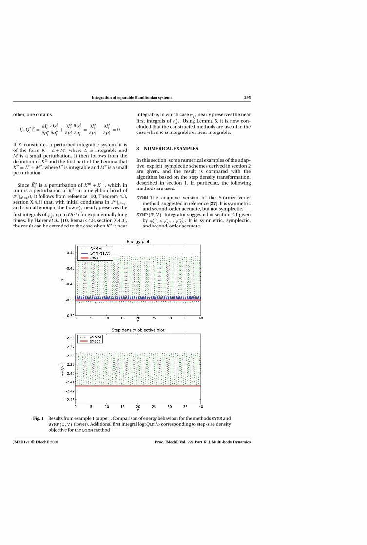
Integration of separable Hamiltonian systems 295
other, one obtains
{I 2i , Q2
j }2 = ∂I 2i
∂p0j
∂Q2j
∂q0j
+ ∂I 2i
∂p1j
∂Q2j
∂q1j
= ∂I 2i
∂p0j
− ∂I 2i
∂p1j
= 0
If K constitutes a perturbed integrable system, it isof the form K = L + M , where L is integrable andM is a small perturbation. It then follows from thedefinition of K 2 and the first part of the Lemma thatK 2 = L2 + M 2, where L2 is integrable and M 2 is a smallperturbation.
Since K 2ε is a perturbation of K 01 + K 10, which in
turn is a perturbation of K 2 (in a neighbourhood ofP 2|z0=z1 ), it follows from reference [10, Theorem 4.3,section X.4.3] that, with initial conditions in P 2|z0=z1
and ε small enough, the flow ϕτ
K 2ε
nearly preserves the
first integrals of ϕτK 2 up to O(εr) for exponentially long
times. By Hairer et al. [10, Remark 4.8, section X.4.3],the result can be extended to the case when K 2 is near
integrable, in which case ϕτ
K 2ε
nearly preserves the nearfirst integrals of ϕτ
K 2 . Using Lemma 5, it is now con-cluded that the constructed methods are useful in thecase when K is integrable or near integrable.
3 NUMERICAL EXAMPLES
In this section, some numerical examples of the adap-tive, explicit, symplectic schemes derived in section 2are given, and the result is compared with thealgorithm based on the step density transformation,described in section 1. In particular, the followingmethods are used.
SYMM The adaptive version of the Störmer–Verletmethod, suggested in reference [27]. It is symmetricand second-order accurate, but not symplectic.
SYMP(T,V) Integrator suggested in section 2.1 givenby ϕε/2
U ,V ◦ ϕεS,T ◦ ϕε/2
U ,V . It is symmetric, symplectic,and second-order accurate.
Fig. 1 Results from example 1 (upper). Comparison of energy behaviour for the methodsSYMM andSYMP(T,V) (lower). Additional first integral log(Q(z)/� corresponding to step-size densityobjective for the SYMM method
JMBD171 © IMechE 2008 Proc. IMechE Vol. 222 Part K: J. Multi-body Dynamics
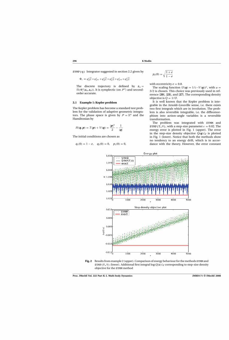
296 K Modin
SYMP(q) Integrator suggested in section 2.2 given by
�ε = ϕε/2E01 ◦ ϕε
F 01 ◦ ϕε/2E01 ◦ ϕε/2
E10 ◦ ϕεF 10 ◦ ϕε/2
E10
The discrete trajectory is defined by zn =�(�n
ε (z0, z0)). It is symplectic (on P 2) and second-order accurate.
3.1 Example 1: Kepler problem
The Kepler problem has become a standard test prob-lem for the validation of adaptive geometric integra-tors. The phase space is given by P = R
4 and theHamiltonian by
H (q, p) = T (p) + V (q) = |p|2
2− 1
|q|The initial conditions are chosen as
q1(0) = 1 − e, q2(0) = 0, p1(0) = 0,
p2(0) =√
1 + e1 − e
with eccentricity e = 0.8.The scaling function U (q) = 1/(−V (q))α, with α =
3/2 is chosen. This choice was previously used in ref-erence [20], [23], and [27]. The corresponding densityobjective is Q = 1/U .
It is well known that the Kepler problem is inte-grable in the Arnold–Liouville sense, i.e. there existstwo first integrals which are in involution. The prob-lem is also reversible integrable, i.e. the diffeomor-phism into action–angle variables is a reversibletransformation.
The problem was integrated with SYMM andSYMP(T,V), with a step-size parameter ε = 0.02. Theenergy error is plotted in Fig. 1 (upper). The errorin the step-size density objective Q(q)/� is plottedin Fig. 1 (lower). Notice that both the methods showno tendency to an energy drift, which is in accor-dance with the theory. However, the error constant
Fig. 2 Results from example 2 (upper). Comparison of energy behaviour for the methodsSYMM andSYMP(T,V) (lower). Additional first integral log(Q(z)/� corresponding to step-size densityobjective for the SYMM method
Proc. IMechE Vol. 222 Part K: J. Multi-body Dynamics JMBD171 © IMechE 2008
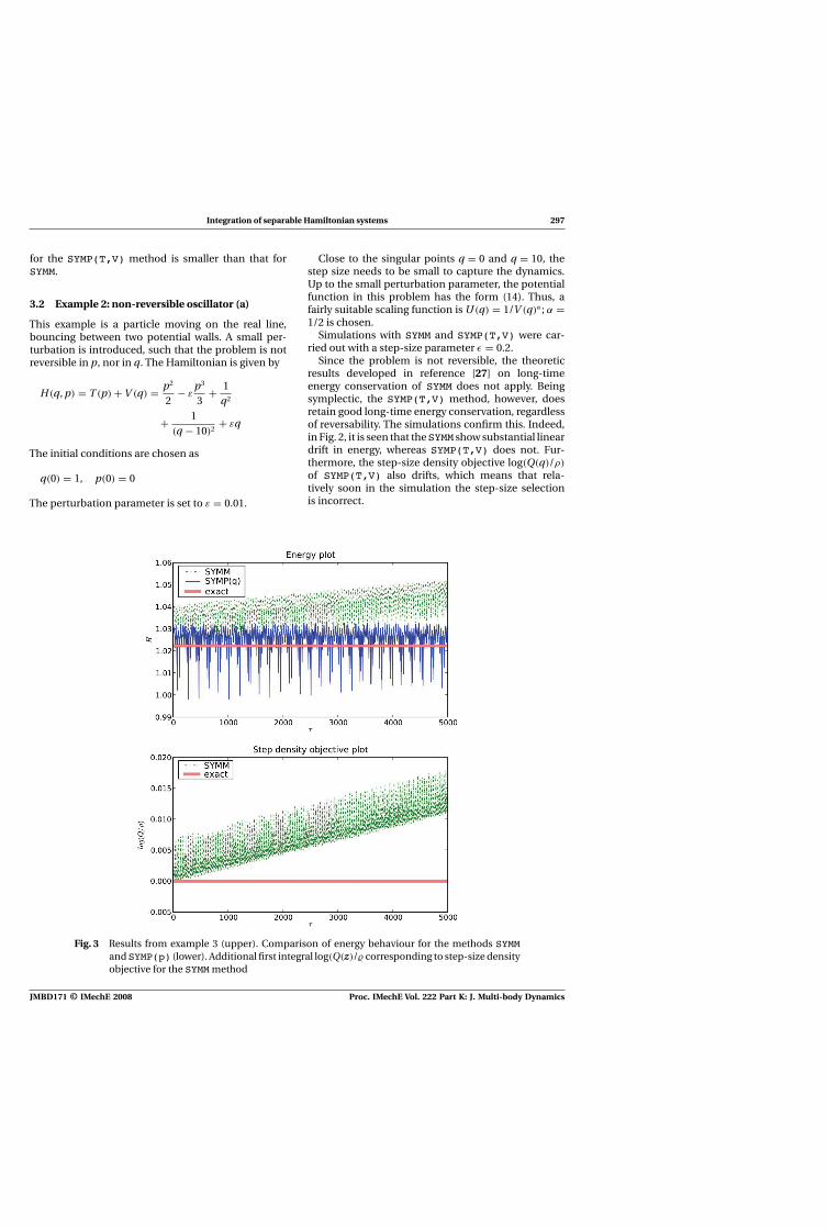
Integration of separable Hamiltonian systems 297
for the SYMP(T,V) method is smaller than that forSYMM.
3.2 Example 2: non-reversible oscillator (a)
This example is a particle moving on the real line,bouncing between two potential walls. A small per-turbation is introduced, such that the problem is notreversible in p, nor in q. The Hamiltonian is given by
H (q, p) = T (p) + V (q) = p2
2− ε
p3
3+ 1
q2
+ 1(q − 10)2
+ εq
The initial conditions are chosen as
q(0) = 1, p(0) = 0
The perturbation parameter is set to ε = 0.01.
Close to the singular points q = 0 and q = 10, thestep size needs to be small to capture the dynamics.Up to the small perturbation parameter, the potentialfunction in this problem has the form (14). Thus, afairly suitable scaling function is U (q) = 1/V (q)α; α =1/2 is chosen.
Simulations with SYMM and SYMP(T,V) were car-ried out with a step-size parameter ε = 0.2.
Since the problem is not reversible, the theoreticresults developed in reference [27] on long-timeenergy conservation of SYMM does not apply. Beingsymplectic, the SYMP(T,V) method, however, doesretain good long-time energy conservation, regardlessof reversability. The simulations confirm this. Indeed,in Fig. 2, it is seen that theSYMM show substantial lineardrift in energy, whereas SYMP(T,V) does not. Fur-thermore, the step-size density objective log(Q(q)/ρ)
of SYMP(T,V) also drifts, which means that rela-tively soon in the simulation the step-size selectionis incorrect.
Fig. 3 Results from example 3 (upper). Comparison of energy behaviour for the methods SYMMandSYMP(p) (lower). Additional first integral log(Q(z)/� corresponding to step-size densityobjective for the SYMM method
JMBD171 © IMechE 2008 Proc. IMechE Vol. 222 Part K: J. Multi-body Dynamics
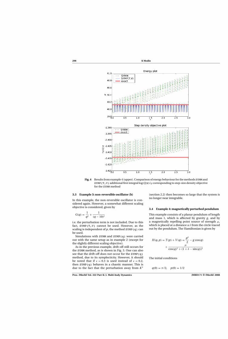
298 K Modin
Fig. 4 Results from example 4 (upper). Comparison of energy behaviour for the methodsSYMM andSYMP(T,V) additional first integral log(Q(z)/� corresponding to step-size density objectivefor the SYMM method
3.3 Example 3: non-reversible oscillator (b)
In this example, the non-reversible oscillator is con-sidered again. However, a somewhat different scalingobjective is considered, given by
G(q) = 1q2
+ 1(q − 10)2
i.e. the perturbation term is not included. Due to thisfact, SYMP(T,V) cannot be used. However, as thescaling is independent of p, the method SYMP(q) canbe used.
Simulations with SYMM and SYMP(q) were carriedout with the same setup as in example 2 (except forthe slightly different scaling objective).
As in the previous example, drift-off still occurs forthe SYMM method, as is shown in Fig. 3. One can alsosee that the drift-off does not occur for the SYMP(q)method, due to its symplecticity. However, it shouldbe noted that if ε = 0.3 is used instead of ε = 0.2,then SYMP(q) behaves in a chaotic manner. This isdue to the fact that the perturbation away from K 2
(section 2.2) then becomes so large that the system isno longer near integrable.
3.4 Example 4: magnetically perturbed pendulum
This example consists of a planar pendulum of lengthand mass 1, which is affected by gravity g , and bya magnetically repelling point source of strength μ,which is placed at a distance a δ from the circle tracedout by the pendulum. The Hamiltonian is given by
H (q, p) = T (p) + V (q) = p2
2− g cos(q)
+ μ
cos(q)2 + (1 + δ − sin(q))2
The initial conditions
q(0) = π/2, p(0) = 1/2
Proc. IMechE Vol. 222 Part K: J. Multi-body Dynamics JMBD171 © IMechE 2008
Integration of separable Hamiltonian systems 299
are chosen such that the kinetic energy is large enoughfor the pendulum to keep rotating in the same direc-tion. Gravity is set to g = 1, and the magnetic sourceat distance δ = 0.05 with strength μ = 0.1.
Again, the scaling function is chosen as U (q) =1/V (q)α, with α = 1/2, which corresponds to smallsteps near the magnetic point source, disregarding theg cos(q) term. Simulations with SYMM and SYMP(T,V)were carried out with step-size parameter ε = 0.001.
Notice that the problem is reversible, i.e. T (p) =T (−p). However, as the pendulum is rotating in thesame direction all the time, one always obtains p >
0, which means that reversibility is ‘not seen’. So,even though the problem is reversible, the reversiblemethod SYMM has drift both in energy and in thestep-size density objective, as is shown in Fig. 4. Thesymplectic method SYMP(T,V) behaves according totheory, i.e. there is no energy drift.
4 CONCLUSIONS
Based on splitting, two approaches for explicit, adap-tive, and symplectic integration of separable Hamilto-nian problems have been developed for two familiesof scaling functions. Second-order versions of the inte-grators have been compared with the state-of-the-artexplicit, adaptive, reversible integrator suggested inreference [27], for four example problems. For non-reversible problems, or reversible problems wherereversability is ‘not shown’, the proposed integratorshave superior long-time energy behaviour.
ACKNOWLEDGEMENTS
The author is grateful to Dag Fritzson, Claus Führer,and Gustaf Söderlind for helpful and inspiring discus-sions. The author would also like to thank SKF for thesupport given.
REFERENCES
1 Newton, I. Philosophiae naturalis principia mathemat-ica, Londini anno MDCLXXXVII, 1687.
2 Euler, L. Decouverte d’un nouveau principe de meca-nique. Mémoires de l’académie des sciences de Berlin,1752, 6, 185–217.
3 Dugas, R. A history of mechanics, 1988 (Dover Publi-cations Inc., New York). (With a foreword by Louis de
Broglie, Translated from the French by J. R. Maddox,Reprint of the 1957 translation).
4 Lagrange, J. L. Mécanique analytique, 1788 (Paris).5 Arnold, V. I. Mathematical methods of classical mechan-
ics, Graduate texts in mathematics, 2nd edition, vol. 60,1989 (Springer-Verlag, New York). (Translated from theRussian by K. Vogtmann and A. Weinstein).
6 Hamilton, S. W. R. First essay on a general method indynamics, 1834 (Royal Society of London PhilosophicalTransactions, London).
7 Hamilton, S. W. R. Second essay on a general method indynamics, 1835 (Royal Society of London PhilosophicalTransactions, London).
8 Marsden J. E. and Ratiu, T. S. Introduction to mechanicsand symmetry, vol. 17 of texts in applied mathematics,2nd edition, 1999 (Springer-Verlag, New York).
9 Holm, D. D. Geometric mechanics. Part I, 2008 (ImperialCollege Press, London).
10 Hairer, E., Lubich, C., and Wanner, G. Geometric numer-ical integration, vol. 31 of Springer Series in Computa-tional Mathematics, 2nd edition, 2006 (Springer-Verlag,Berlin).
11 Faou, E., Hairer, E., and Pham,T.-L. Energy conservationwith non-symplectic methods: examples and counter-examples. BIT, 2004, 44(4), 699–709.
12 McLachlan, R. I. and Perlmutter, M. Energy drift inreversible time integration. J. Phys. A, 2004, 37(45),L593–L598.
13 Yoshida, H. Construction of higher order symplecticintegrators. Phys. Lett. A, 1990, 150(5–7), 262–268.
14 Murua, A. and Sanz-Serna, J. M. Order conditions fornumerical integrators obtained by composing simplerintegrators. R. Soc. Lond. Philos. Trans. Ser. A Math. Phys.Eng. Sci., 1999, 357(1754), 1079–1100.
15 McLachlan, R. I. and Quispel, G. R. W. Splitting methods.Acta Numer., 2002, 11, 341–434.
16 Gladman, B., Duncan, M., and Candy, J. Symplecticintegrators for long-term integrations in celestial mech-anics. Celestial Mech. Dynam. Astronom., 1991, 52(3),221–240.
17 Calvo, M. P. and Sanz-Serna, J. M. Variable steps for sym-plectic integrators. In Numerical analysis 1991 (Dundee,1991), Pitman Research in Notes Mathematical Series,vol. 260, 1992, pp. 34–48 (Longman Scientific &Technical,Harlow).
18 Huang, W. and Leimkuhler, B. The adaptive Verletmethod. SIAM J. Sci. Comput., 1997, 18(1), 239–256.
19 Stoffer, D. Variable steps for reversible integration meth-ods. Computing, 1995, 55(1), 1–22.
20 Hairer, E. Variable time step integration with symplecticmethods. Appl. Numer. Math., 1997, 25(2–3), 219–227.
21 Reich, S. Backward error analysis for numerical integra-tors. SIAM J. Numer. Anal., 1999, 36(5), 1549–1570.
22 Mikkola, S. and Wiegert, P. Regularizing time trans-formations in symplectic and composite integra-tion. Celestial Mech. Dynam. Astronom., 2002, 82(4),375–390.
23 Blanes, S. and Budd, C. J. Explicit adaptive sym-plectic (easy) integrators: a scaling invariant gen-eralisation of the Levi-Civita and KS regularisa-tions. Celestial Mech. Dynam. Astronom., 2004, 89(4),383–405.
JMBD171 © IMechE 2008 Proc. IMechE Vol. 222 Part K: J. Multi-body Dynamics
300 K Modin
24 Blanes, S. and Budd, C. J. Adaptive geometric inte-grators for Hamiltonian problems with approximatescale invariance. SIAM J. Sci. Comput., 2005, 26(4),1089–1113.
25 Modin, K. and Führer, C. Time-step adaptivity in varia-tional integrators with application to contact problems.ZAMM Z. Angew. Math. Mech., 2006, 86(10), 785–794.
26 Marsden, J. E. and West, M. Discrete mechanics andvariational integrators. Acta Numer., 2001, 10, 357–514.
27 Hairer, E. and Söderlind, G. Explicit, time reversible,adaptive step size control. SIAM J. Sci. Comput., 2005,26(6), 1838–1851.
28 Preto, M. and Tremaine, S. A class of symplectic integra-tors with adaptive timestep for separable hamiltoniansystems. Astron. J., 1999, 118 (5), 2532–2541.
29 Zare, K. and Szebehely, V. Time transformations inthe extended phase-space, Celestial Mech., 1975, 11,pp. 469–482.
Proc. IMechE Vol. 222 Part K: J. Multi-body Dynamics JMBD171 © IMechE 2008

Paper IV
Klas Modin.J. Gen. Lie Theory Appl., 3(1):39–52, 2009.

Journal of Generalized Lie Theory and Applications Vol. 3 (2009), No. 1, 39–52
Time transformation and reversibility of
Nambu–Poisson systems
Klas MODIN a,b
a Centre for Mathematical Sciences, Lund University, Box 118, SE–221 00 Lund, Sweden
E-mail: [email protected] SKF Engineering & Research Centre, MDC, RKs–2, SE–415 50 Goteborg, Sweden
Abstract
A time transformation technique for Nambu–Poisson systems is developed, and its struc-tural properties are examined. The approach is based on extension of the phase space P
into P = P×R, where the additional variable controls the time-stretching rate. It is shownthat time transformation of a system on P can be realised as an extended system on P,with an extended Nambu–Poisson structure. In addition, reversible systems are studied inconjunction with the Nambu–Poisson structure. The application in mind is adaptive nu-merical integration by splitting of Nambu–Poisson Hamiltonians. As an example, a novelintegration method for the rigid body problem is presented and analysed.
2000 MSC: 37M99, 22E70, 53Z05, 34A26
1 Introduction
In 1973 Nambu [23] suggested a generalisation of Hamiltonian mechanics, taking the Liouvillecondition on volume preservation in phase space as a governing principle. Nambu postulatedthat the governing equations for a dynamical system on R
n should have the form
dxi
dt=
∑j1,...,jn−1
εij1...jn−1
∂H1
∂xj1
∂H2
∂xj2
. . .∂Hn−1
∂xjn−1
(1.1)
where ε is the Levi–Civita tensor over n indices, and H1, . . . ,Hn−1 are smooth real valuedfunctions on R
n called Hamiltonian functions. Notice that the vector field in equation (1.1) issource free (its divergence is zero), which implies that the corresponding phase flow is volumepreserving.
Later Takhtajan [27] formalised Nambu’s framework by introducing the concept of Nambu–Poisson brackets on general phase space manifolds. Based on Takhtajan’s work the geometry ofNambu–Poisson structures has been explored in several papers [6, 4, 5, 21, 11, 22, 28, 29].
In this paper we study time transformation of Nambu–Poisson systems. Such transformationsare important in the construction and analysis of adaptive structure preserving numerical timestepping methods [26, 10, 3, 7, 24, 18, 2, 20, 19]. The idea is to obtain time step adaptivityby equidistant discretisation in the transformed variable, which corresponds to non-equidistantdiscretisation in the original time variable. Although numerical integration is a main motivation,the focus in the paper is not on numerical issues, but rather on structural properties.
The current section continues with a brief review of Nambu–Poisson mechanics, and of a timetransformation method by Hairer and Soderlind [9]. The main results are in Section 2, wheretime transformation for Nambu–Poisson systems is developed. In Section 3, the Nambu–Poisson
40 Klas Modin
structure is studied in conjunction with reversibility. As an application, we show in Section 4how to construct fully explicit, adaptive numerical integration methods based on splitting of theNambu–Poisson Hamiltonians. In particular, a novel method for the free rigid body. Conclusionsare given in Section 5.
We adopt the following notation. P denotes a phase space manifold of dimension n, withlocal coordinates x = (x1, . . . , xn). The algebra of smooth real valued functions on P is de-noted F(P). Further, X(P) denotes the linear space of vector fields on P. The Lie derivativealong X ∈ X(P) is denoted LX . If X,Y ∈ X(P) then the commutator [X,Y ] = LXY sup-plies X(P) with an infinite dimensional Lie algebra structure. Its corresponding Lie group isthe set Diff(P) of diffeomorphisms on P, with composition as group operation. (See McLach-lan and Quispel [16] and Schmid [25] for issues concerning infinite dimensional Lie groups.)If Φ ∈ Diff(P) then Φ∗ denotes the pull-back map and Φ∗ the push-forward map imposed by Φ.
1.1 Nambu–Poisson mechanics
In Hamiltonian mechanics, the phase space manifold P is equipped with a Poisson structure,defined by a bracket operation {·1, ·2} : F(P) ×F(P) → F(P) that is skew-symmetric, fulfilsthe Leibniz rule and the Jacobi identity. Nambu–Poisson mechanics is a generalisation.
Definition 1.1. A Nambu–Poisson manifold of order k consists of a smooth manifold P togetherwith a multilinear map
{·1, . . . , ·k} : F(P) × . . . ×F(P)︸ ︷︷ ︸k times
→ F(P)
that fulfils:
• total skew-symmetry
{H1, . . . ,Hk} = sgn(σ){Hσ1 , . . . ,Hσk} (1.2a)
• Leibniz rule
{GH1, . . . ,Hk} = G{H1, . . . ,Hm} + H1{G,H2, . . . ,Hk} (1.2b)
• fundamental identity
{H1, . . . ,Hk−1, {G1, . . . , Gk}} = {{H1, . . . ,Hk−1, G1}, G2, . . . , Gk}
+ {G1, {H1, . . . ,Hk−1, G2}, G3, . . . , Gk} + . . .
+ {G1, . . . , Gk−1, {H1, . . . ,Hk−1, Gk}} (1.2c)
Remark 1.1. The case k = 2 coincides with ordinary Poisson manifolds.
The first two conditions, total skew-symmetry (1.2a) and Leibniz rule (1.2b), are straightfor-ward: they imply that the bracket is of the form
{H1, . . . ,Hk} = η(dH1, . . . , dHk)
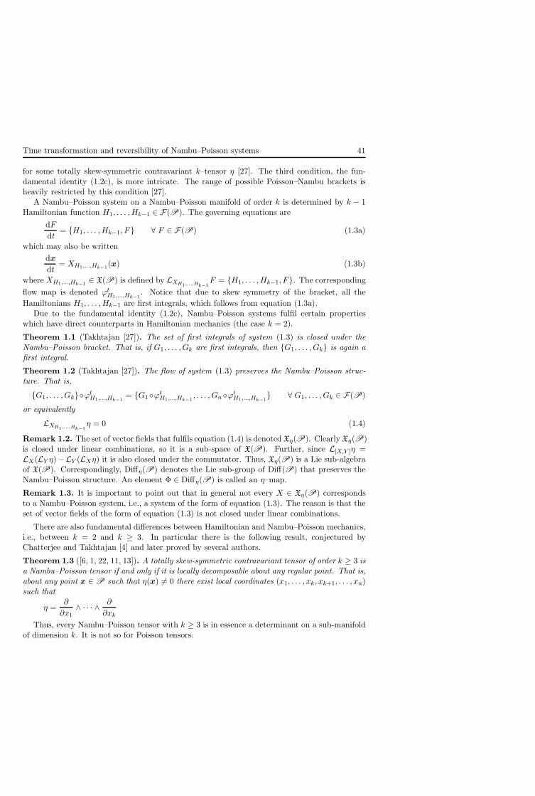
Time transformation and reversibility of Nambu–Poisson systems 41
for some totally skew-symmetric contravariant k–tensor η [27]. The third condition, the fun-damental identity (1.2c), is more intricate. The range of possible Poisson–Nambu brackets isheavily restricted by this condition [27].
A Nambu–Poisson system on a Nambu–Poisson manifold of order k is determined by k − 1Hamiltonian function H1, . . . ,Hk−1 ∈ F(P). The governing equations are
dF
dt= {H1, . . . ,Hk−1, F} ∀ F ∈ F(P) (1.3a)
which may also be writtendx
dt= XH1,...,Hk−1(x) (1.3b)
where XH1,...,Hk−1 ∈ X(P) is defined by LXH1,...,Hk−1F = {H1, . . . ,Hk−1, F}. The corresponding
flow map is denoted ϕtH1,...,Hk−1
. Notice that due to skew symmetry of the bracket, all theHamiltonians H1, . . . ,Hk−1 are first integrals, which follows from equation (1.3a).
Due to the fundamental identity (1.2c), Nambu–Poisson systems fulfil certain propertieswhich have direct counterparts in Hamiltonian mechanics (the case k = 2).
Theorem 1.1 (Takhtajan [27]). The set of first integrals of system (1.3) is closed under the
Nambu–Poisson bracket. That is, if G1, . . . , Gk are first integrals, then {G1, . . . , Gk} is again a
first integral.
Theorem 1.2 (Takhtajan [27]). The flow of system (1.3) preserves the Nambu–Poisson struc-
ture. That is,
{G1, . . . , Gk}◦ϕtH1,...,Hk−1
= {G1 ◦ϕtH1,...,Hk−1
, . . . , Gn ◦ϕtH1,...,Hk−1
} ∀ G1, . . . , Gk ∈ F(P)
or equivalently
LXH1,...,Hk−1η = 0 (1.4)
Remark 1.2. The set of vector fields that fulfils equation (1.4) is denoted Xη(P). Clearly Xη(P)is closed under linear combinations, so it is a sub-space of X(P). Further, since L[X,Y ]η =LX(LY η)−LY (LXη) it is also closed under the commutator. Thus, Xη(P) is a Lie sub-algebraof X(P). Correspondingly, Diffη(P) denotes the Lie sub-group of Diff(P) that preserves theNambu–Poisson structure. An element Φ ∈ Diffη(P) is called an η–map.
Remark 1.3. It is important to point out that in general not every X ∈ Xη(P) correspondsto a Nambu–Poisson system, i.e., a system of the form of equation (1.3). The reason is that theset of vector fields of the form of equation (1.3) is not closed under linear combinations.
There are also fundamental differences between Hamiltonian and Nambu–Poisson mechanics,i.e., between k = 2 and k ≥ 3. In particular there is the following result, conjectured byChatterjee and Takhtajan [4] and later proved by several authors.
Theorem 1.3 ([6, 1, 22, 11, 13]). A totally skew-symmetric contravariant tensor of order k ≥ 3 is
a Nambu–Poisson tensor if and only if it is locally decomposable about any regular point. That is,
about any point x ∈ P such that η(x) �= 0 there exist local coordinates (x1, . . . , xk, xk+1, . . . , xn)such that
η =∂
∂x1∧ · · · ∧
∂
∂xk
Thus, every Nambu–Poisson tensor with k ≥ 3 is in essence a determinant on a sub-manifoldof dimension k. It is not so for Poisson tensors.

42 Klas Modin
1.2 Time transformation of dynamical systems
In this section we review the time transformation technique developed in Hairer and Soderlind [9].Consider a dynamical system
dx
dt= X(x), X ∈ X(P) (1.5)
Its flow map is denoted ϕtX . Introduce an extended phase space P = P × R, with local
coordinates x = (x, ξ). The projection P x → x ∈ P is denoted Π, and P x → ξ ∈ R isdenoted π. Let Q ∈ {F ∈ F(P);F > 0} and consider the extension of system (1.5) into⎧⎪⎨
⎪⎩dx
dτ= X(x)/ξ
dξ
dτ= (LXQ)(x)/Q(x)
or shorterdx
dτ= X(x) (1.6)
The flows of the two systems are related by a reparametrisation t ↔ τ .
Theorem 1.4 (Hairer and Soderlind [9]). The flow of the extended system (1.6) restricted to P
is a time transformation of the flow of system (1.5). That is,
ΠϕτX(x) = ϕ
σ(τ,x)X (x), ∀ x ∈ P , τ ∈ R where σ(τ, x) ≡
∫ τ
0
ds
πϕsX
(x)
Further, Q(x)/ξ is a first integral of system (1.6).
Proof. From equation (1.6) it follows directly that Π∗X is parallel with X. Thus, ΠϕτX
andϕt
X define the same phase diagrams. It remains to find the relation between t and τ . Sincedx/dt = (dt/dτ)(dx/dτ) it follows from equation (1.6) that dt/dτ = 1/ξ. Integration ofthis relation gives σ(τ, x). Further, straightforward calculations and utilisation of the governingequations (1.6) show that d(Q(x)/ξ)/dτ = 0.
Remark 1.4. It is clear that the time transformation is determined by Q. Since Q is strictlypositive, the map σ( · , x) : R → R is bijective, i.e., the reparametrisation t ↔ τ is bijective.
In Hairer and Soderlind [9], the motivation for the extended time transformation (1.6) is toconstruct explicit adaptive numerical integrators for reversible systems. The key is that underreversibility of Q, the extended time transformation (1.6) preserves reversibility. First, recallthe basic definitions of reversible systems.
Definition 1.2. Let R ∈ Diff(P).
• A vector field X ∈ X(P) is called reversible with respect to R if R∗ ◦ X = −X ◦ R, orequivalently d(R(x))/dt = −(X ◦ R)(x).
• A diffeomorphism Φ ∈ Diff(P) is called reversible with respect to R if R ◦ Φ = Φ−1 ◦ R.
It is a well known result that the flow of a system is reversible if and only if its correspondingvector field is reversible [12, 8]. Now, concerning time transformation of reversible systems, it isstraightforward to check the following result.
Theorem 1.5 (Hairer and Soderlind [9]). If X ∈ X(P) is reversible with respect to R and
Q ∈ F(P) fulfils Q = Q ◦R, then the vector field X ∈ X(P) in equation (1.6) is reversible with
respect to R : x → (R(x), ξ).
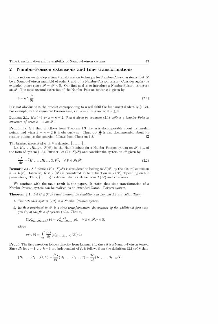
Time transformation and reversibility of Nambu–Poisson systems 43
2 Nambu–Poisson extensions and time transformations
In this section we develop a time transformation technique for Nambu–Poisson systems. Let P
be a Nambu–Poisson manifold of order k and η its Nambu–Poisson tensor. Consider again theextended phase space P = P × R. Our first goal is to introduce a Nambu–Poisson structureon P . The most natural extension of the Nambu–Poisson tensor η is given by
η = η ∧∂
∂ξ(2.1)
It is not obvious that the bracket corresponding to η will fulfil the fundamental identity (1.2c).For example, in the canonical Poisson case, i.e., k = 2, it is not so if n ≥ 3.
Lemma 2.1. If k ≥ 3 or k = n = 2, then η given by equation (2.1) defines a Nambu–Poisson
structure of order k + 1 on P.
Proof. If k ≥ 3 then it follows from Theorem 1.3 that η is decomposable about its regularpoints, and when k = n = 2 it is obviously so. Thus, η ∧ ∂
∂ξ is also decomposable about itsregular points, so the assertion follows from Theorem 1.3.
The bracket associated with η is denoted {·, . . . , ·}.Let H1, . . . ,Hk−1 ∈ F(P) be the Hamiltonians for a Nambu–Poisson system on P, i.e., of
the form of system (1.3). Further, let G ∈ F(P) and consider the system on P given by
dF
dτ= {H1, . . . ,Hk−1, G, F }, ∀ F ∈ F(P) (2.2)
Remark 2.1. A functions H ∈ F(P) is considered to belong to F(P) by the natural extensionx → H(x). Likewise, H ∈ F(P) is considered to be a function in F(P) depending on theparameter ξ. Thus, {·, . . . , ·} is defined also for elements in F(P) and vice versa.
We continue with the main result in the paper. It states that time transformation of aNambu–Poisson system can be realised as an extended Nambu–Poisson system.
Theorem 2.1. Let G ∈ F(P) and assume the conditions in Lemma 2.1 are valid. Then:
1. The extended system (2.2) is a Nambu–Poisson system.
2. Its flow restricted to P is a time transformation, determined by the additional first inte-
gral G, of the flow of system (1.3). That is,
ΠϕτH1,...,Hk−1,G(x) = ϕ
σ(τ,x)H1,...,Hk−1
(x), ∀ x ∈ P , τ ∈ R
where
σ(τ, x) ≡∫ τ
0
∂G
∂ξ
(ϕs
H1,...,Hk−1,G(x))ds
Proof. The first assertion follows directly from Lemma 2.1, since η is a Nambu–Poisson tensor.Since Hi for i = 1, . . . , k − 1 are independent of ξ, it follows from the definition (2.1) of η that
{H1, . . . ,Hk−1, G, F } =∂G
∂ξ{H1, . . . ,Hk−1, F} −
∂F
∂ξ{H1, . . . ,Hk−1, G}
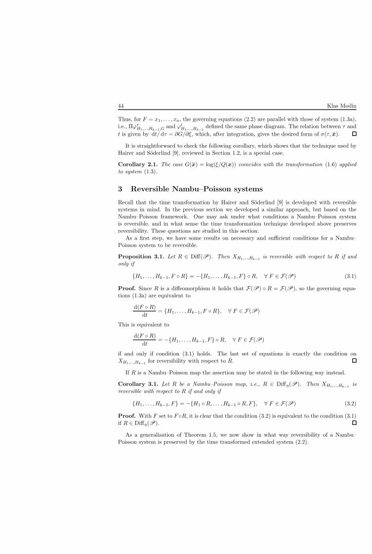
44 Klas Modin
Thus, for F = x1, . . . , xn, the governing equations (2.2) are parallel with those of system (1.3a),i.e., Πϕτ
H1,...,Hk−1,G and ϕtH1,...,Hk−1
defined the same phase diagram. The relation between τ andt is given by dt/dτ = ∂G/∂ξ, which, after integration, gives the desired form of σ(τ, x).
It is straightforward to check the following corollary, which shows that the technique used byHairer and Soderlind [9], reviewed in Section 1.2, is a special case.
Corollary 2.1. The case G(x) = log(ξ/Q(x)) coincides with the transformation (1.6) applied
to system (1.3).
3 Reversible Nambu–Poisson systems
Recall that the time transformation by Hairer and Soderlind [9] is developed with reversiblesystems in mind. In the previous section we developed a similar approach, but based on theNambu–Poisson framework. One may ask under what conditions a Nambu–Poisson systemis reversible, and in what sense the time transformation technique developed above preservesreversibility. These questions are studied in this section.
As a first step, we have some results on necessary and sufficient conditions for a Nambu–Poisson system to be reversible.
Proposition 3.1. Let R ∈ Diff(P). Then XH1,...,Hk−1 is reversible with respect to R if and
only if
{H1, . . . ,Hk−1, F ◦ R} = −{H1, . . . ,Hk−1, F} ◦ R, ∀ F ∈ F(P) (3.1)
Proof. Since R is a diffeomorphism it holds that F(P) ◦ R = F(P), so the governing equa-tions (1.3a) are equivalent to
d(F ◦ R)dt
= {H1, . . . ,Hk−1, F ◦ R}, ∀ F ∈ F(P)
This is equivalent to
d(F ◦ R)dt
= −{H1, . . . ,Hk−1, F} ◦ R, ∀ F ∈ F(P)
if and only if condition (3.1) holds. The last set of equations is exactly the condition onXH1,...,Hk−1 for reversibility with respect to R.
If R is a Nambu–Poisson map the assertion may be stated in the following way instead.
Corollary 3.1. Let R be a Nambu–Poisson map, i.e., R ∈ Diffη(P). Then XH1,...,Hk−1 is
reversible with respect to R if and only if
{H1, . . . ,Hk−1, F} = −{H1 ◦ R, . . . ,Hk−1 ◦ R,F}, ∀ F ∈ F(P) (3.2)
Proof. With F set to F ◦R, it is clear that the condition (3.2) is equivalent to the condition (3.1)if R ∈ Diffη(P).
As a generalisation of Theorem 1.5, we now show in what way reversibility of a Nambu–Poisson system is preserved by the time transformed extended system (2.2).
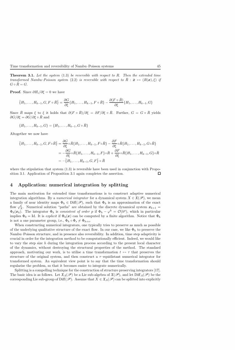
Time transformation and reversibility of Nambu–Poisson systems 45
Theorem 3.1. Let the system (1.3) be reversible with respect to R. Then the extended time
transformed Nambu–Poisson system (2.2) is reversible with respect to R : x → (R(x), ξ) if
G ◦ R = G.
Proof. Since ∂Hi/∂ξ = 0 we have
{H1, . . . ,Hk−1, G, F ◦ R} =∂G
∂ξ{H1, . . . ,Hk−1, F ◦ R} −
∂(F ◦ R)∂ξ
{H1, . . . ,Hk−1, G}
Since R maps ξ to ξ it holds that ∂(F ◦ R)/∂ξ = ∂F/∂ξ ◦ R. Further, G = G ◦ R yields∂G/∂ξ = ∂G/∂ξ ◦ R and
{H1, . . . ,Hk−1, G} = {H1, . . . ,Hk−1, G ◦ R}
Altogether we now have
{H1, . . . ,Hk−1, G, F ◦R} =∂G
∂ξ◦R{H1, . . . ,Hk−1, F ◦R} −
∂F
∂ξ◦R{H1, . . . ,Hk−1, G◦R}
= −∂G
∂ξ◦R{H1, . . . ,Hk−1, F}◦R +
∂F
∂ξ◦R{H1, . . . ,Hk−1, G}◦R
= −{H1, . . . ,Hk−1, G, F } ◦ R
where the stipulation that system (1.3) is reversible have been used in conjunction with Propo-sition 3.1. Application of Proposition 3.1 again completes the assertion.
4 Application: numerical integration by splitting
The main motivation for extended time transformations is to construct adaptive numericalintegration algorithms. By a numerical integrator for a dynamical system X ∈ X(P), we meana family of near identity maps Φh ∈ Diff(P), such that Φh is an approximation of the exactflow ϕh
X . Numerical solution “paths” are obtained by the discrete dynamical system xk+1 =Φh(xk). The integrator Φh is consistent of order p if Φh − ϕh = O(hp), which in particularimplies Φ0 = Id. It is explicit if Φh(x) can be computed by a finite algorithm. Notice that Φh
is not a one parameter group, i.e., Φh ◦ Φs �= Φh+s.When constructing numerical integrators, one typically tries to preserve as much as possible
of the underlying qualitative structure of the exact flow. In our case, we like Φh to preserve theNambu–Poisson structure, and in presence also reversibility. In addition, time step adaptivity iscrucial in order for the integration method to be computationally efficient. Indeed, we would liketo vary the step size h during the integration process according to the present local characterof the dynamics, without destroying the structural properties of the method. The standardapproach, motivating our work, is to utilise a time transformation t ↔ τ that preserves thestructure of the original system, and then construct a τ–equidistant numerical integrator fortransformed system. An equivalent view point is to say that the time transformation shouldregularise the problem, so that it becomes easier to integrate numerically.
Splitting is a compelling technique for the construction of structure preserving integrators [17].The basic idea is as follows. Let XA(P) be a Lie sub-algebra of X(P), and let DiffA(P) be thecorresponding Lie sub-group of Diff(P). Assume that X ∈ XA(P) can be splitted into explicitly
46 Klas Modin
integrable sub-system, each of which is a system in XA(P). That is, X = X1 + . . . + Xk, whereXi ∈ XA(P) and ϕt
Xi(x) can be computed explicitly. A numerical integrator for X is obtained
by Φh = ϕhX1
◦· · · ◦ϕhXk
. It is clear that Φh is an approximation of ϕhX , and that Φh ∈ DiffA(P).
Further, by the Baker–Campbell–Hausdorff (BCH) formula, it follows that Φh is the exact flow ofa modified vector field Xh ∈ XA(P), i.e., Φh = ϕh
Xh. This information is crucial for the analysis
of Φh. For example, if XA(P) is the Lie-algebra corresponding to a Poisson structure on P,then Φh will exactly conserve a modified Hamiltonian, which is O(hp)–close to the Hamiltonianfor the original problem [8].
Remark 4.1. Due to convergence issues, the BCH formula needs to be truncated, which impliesthat assertions on Φh, coming from X, are valid only for exponentially long times, i.e., up totime scales of order O(exp(O(1/hp))). See Hairer et. al. [8] for details.
Our notion for the construction of integrators is to utilise the results in Section 2–3, andconsider splitting of the individual Nambu–Poisson Hamiltonians.
Let η be a Nambu–Poisson tensor. The set of Nambu–Poisson maps which are reversible withrespect to R is denoted Diffη,R(P). If Φ,Ψ ∈ Diffη,R(P), then in general we have
R ◦ Φ ◦ Ψ = Φ−1 ◦ R ◦ Ψ = Φ−1 ◦ Ψ−1 ◦ R �= (Φ ◦ Ψ)−1 ◦ R
Thus, Diffη,R(P) is not closed under composition, so it is not a sub-group of Diff(P). However,Diffη,R(P) is closed under the symmetric group operation (Φ,Ψ) →
√Φ◦Ψ◦
√Φ, which we write
as Φ�Ψ. Further, from the symmetric BCH formula (cf. [15]) it follows that if X,Y ∈ Xη,R(P),then the vector field Z such that ϕt
Z = ϕtX � ϕt
Y belongs to Xη,R(P).
Remark 4.2. For near identity maps,√
Φ is defined by taking its representation Φ = exp(X)and then setting
√Φ = exp(X/2). In our case, Φ will always be an exact flow ϕt
X , in which case√ϕt
X = ϕt/2X .
We now give a result concerning reversible systems, which is of use for the analysis of periodicnumerical paths of reversible splitting methods.
Lemma 4.1. Let X ∈ X(P) be reversible with respect to R ∈ Diff(P). Assume that the set
U = {x ∈ P;R(x) = x} of fix-points of R is non-empty and that γ : R → P is a solution curve
of X for which there exists t1, t2 ∈ R with t1 < t2 such that γ(t1), γ(t2) ∈ U. Then γ is periodic.
γ2 γ
U
Proof. For simplicity assume that t1 = 0 and t2 > 0, which is not arestriction. The curve γ2(t) = (R ◦ γ)(−t) is also a solution curve due toreversibility. Further, since R restricted to U is the identity map we havethe equalities γ(t1) = γ2(t1) and γ(−t2) = γ2(t2). Due to uniqueness ofsolutions the first equality implies γ2 = γ, which in conjunction with thesecond equality implies that γ(−t2) = γ(t2). Thus γ returns to the samepoint twice, so it is periodic.
4.1 Rigid body problem
The Euler equations for the free rigid body is a Nambu–Poisson system on the phase space R3,
equipped with the canonical Nambu–Poisson structure η = ∂/∂x1 ∧ ∂/∂x2 ∧ ∂/∂x3. Its two
Time transformation and reversibility of Nambu–Poisson systems 47
Hamiltonians are total angular momentum M(x) =∑
x2i /2 and kinetic energy T (x) =
∑x2
i /(2Ii),where Ii > 0 are the principal moments of inertia. Thus, the governing equations are
dF
dt= {M,T, F}, ∀ F ∈ F(R3) (4.1a)
which explicitly reads
x1 = a1x2x3, a1 = (I2 − I3)/(I2I3)x2 = a2x3x1, a2 = (I3 − I1)/(I3I1)x3 = a3x1x2, a3 = (I1 − I2)/(I1I2)
(4.1b)
It is straightforward to check that the system is reversible with respect to the linear diffeomor-phism R1 : x → (−x1, x2, x3), and in symmetry, also with respect to R2, R3 defined analogously.Thus, due to Lemma 4.1, we have the following KAM–like result for the free rigid body.
Theorem 4.1. Let Xh ∈ X(R3) depend smoothly on h such that X0 = XM,T �= 0. Assume
that Xh, for each h, is reversible with respect to R1, R2 and R3. Then, for small enough h, the
solution paths of Xh are periodic.
Proof. It is known that if γ is a solution curve of the Euler equations, then it is either anequilibrium, or it is periodic with finite period te > 0, in which case it crosses either of the planesUi = {x ∈ R
3;Ri(x) = x} every half period [14]. That is, it holds that γ(t1), γ(t1 + te/2) ∈ Uk
for some k ∈ {1, 2, 3} and t1 ∈ [0, te/2). Further, since XM,T ≡ 0 is not allowed, it is known thatif γ is an equilibrium, then γ(t) ∈ Uk. Let γh be a solution curve of Xh and let γ be the solutioncurve of XM,T such that γ(0) = γh(0). Assume first that γ is not an equilibrium. Then, forany δ ∈ (0, te/2) it holds that a continuous path between γ(t1 − δ) and γ(t1 + δ) must cross theplane Uk. For small enough h it holds that γh(t1 − δ) and γh(t1 + δ) approximates γ(t1 − δ) andγ(t1 + δ) well enough to also be separated by Uk. Thus, γh(t1) ∈ U1 for some t1 ∈ (t1− δ, t1 + δ).Likewise, γh(t2) ∈ U1 for some t2 ∈ (t1 + te/2 − δ, t1 + te/2 + δ). Since Xh is reversible withrespect to R1 it follows from Lemma 4.1 that γh is periodic. If γ is an equilibrium and γh is not,then either there exists s > 0 such that γh(s) /∈ Uk, in which case the solution curve of XM,T
such that γ(s) = γh(s) is periodic, so we are back to the first case, or γh(0), γh(s) ∈ Uk, in whichcase the assertion follows directly from Lemma 4.1.
The traditional perception in the literature is to view the rigid body equations (4.1) asa Poisson system, with the non-canonical Poisson tensor ηM = η(dM, ·1, ·2), induced by thetotal angular momentum (M is a Casimir, cf. [14], for this Poisson structure). We denote thecorresponding bracket by {·1, ·2}M . It is clear that DiffηM
is a sub-group of Diffη. Consider theHamiltonian splitting T =
∑Ti, where Ti(x) = x2
i /(2Ii). The sub-system F = {Ti, F}M doesnot affect xi, i.e., xi = 0, and all the quadratic terms contain xi. Hence, it is in essence a linearsystem on R
2, and therefore explicitly integrable (since the exponential map is computablefor any 2 × 2–matrix). A well known second order integrator is obtained by the symmetriccomposition
Φ�Th = ϕh
M,T1� ϕh
M,T2� ϕh
M,T3
This integrator has the following properties:
48 Klas Modin
1. It is reversible with respect to R1, R2 and R3. Thus, its modified vector field Xh is aR1, R2, R3–reversible perturbation of X, so Theorem 4.1 may be used to deduce periodicorbits of the numerical solution.
2. It is a Poisson map, i.e., Φ�Th ∈ DiffηM
(P). This implies that its modified vector field Xh
is the Hamiltonian vector field of a modified Hamiltonian Th = T + O(h2), so T is nearlyconserved. Further, since M is a Casimir of the Poisson structure it is exactly conserved.
Remark 4.3. One may also view the rigid body equations (4.1) as a Poisson system with thePoisson tensor ηT = η(·1, dT, ·2), and then construct an integrator Φ
�Mh by splitting of M . This
integrator will exactly conserve T , and nearly conserve M .
Following our notion, we now consider Hamiltonian splitting of both M and T . To this end,let Mi(x) = x2
i /2. Since XMi,Ti= 0 it follows that
XM,T = XM1+M2,T1+T2 + XM2+M3,T2+T3 + XM3+M1,T3+T1
Each such vector field is integrable by linear extrapolation, for example,
ϕtM1+M2,T1+T2
(x) = x + tXM1+M2,T1+T2(x)
Thus, a second order integrator is obtained by
Φ�M�Th = ϕh
M1+M2,T1+T2� ϕh
M2+M3,T2+T3� ϕh
M3+M1,T3+T1
This integrator is computationally cheaper than Φ�Th , since computation of the exponential map,
which involves evaluation of sin and cos, is not necessary. Further, it has the following properties:
1. It is reversible with respect to R1, R2 and R3. Thus, its modified vector field Xh isa R1, R2, R3–reversible perturbation of XM,T , so Theorem 4.1 may be used to deduceperiodic orbits of the numerical solution.
2. It is an η–map, i.e., Φ�M�Th ∈ Diffη, which implies X ∈ Xη(P). However, Φ
�M�Th does
not correspond to a modified Nambu–Poisson system (see Remark 1.3), so there are noexactly conserved modified Hamiltonians M and T . Nevertheless, M and T are still nearlyconserved due to the periodicity of the numerical solution.
Consider now time transformation of system (4.1) into an extended Nambu–Poisson system
dF
dτ= {M,T,G,F }, ∀F ∈ F(R4) (4.2)
We have the following generalisation of Theorem 4.1.
Theorem 4.2. Let Xε ∈ X(R4) depend smoothly on ε such that X0 = XM,T,G �= 0. Assume that
Xε, for each ε, is reversible with respect to R1, R2 and R3, and that there exists δ > 0 such that
∂G/∂ξ > δ. Then, for small enough ε, the solution paths of Xε are periodic.
Proof. From the definition of Ri it follows that Ui = {x ∈ R4; Ri(x) = x} is a hyper-plane,
and that R3 x ∈ Ui implies (x, ξ) ∈ Ui for all ξ ∈ R. Let γ be a solution curve of XM,T,G.
Since it is a time transformation of a solution curve of XM,T and since ∂G/∂ξ > δ it followsthat there exists t1 < t2 and k ∈ {1, 2, 3} such that γ(t1), γ(t2) ∈ Uk. Thus, γ is periodic due toLemma 4.1. The proof now proceeds exactly as the proof of Theorem 4.1.
Time transformation and reversibility of Nambu–Poisson systems 49
Assume G takes the splitted form G(x) = G1(x)+G2(ξ). We propose the following adaptiveversions of Φ
�Th and Φ
�M�Th .
Φ�T �Gε = ϕε
M,T,G1� ϕε
M,T1,G2� ϕε
M,T2,G2� ϕε
M,T3,G2
Φ�M�T �Gε = ϕε
M,T,G1� ϕε
M1+M2,T1+T2,G2� ϕε
M2+M3,T2+T3,G2� ϕε
M3+M1,T3+T1,G2
Notice that all of the partial flows are explicitly integrable. In particular, ϕεM,T,G1
(x) = x +εXM,T,G1(x). Further, it holds that
ϕεM,Ti,G2
(x) = (ϕε
∂G2∂ξ
(ξ)
M,Ti(x), 0), i = 1, 2, 3
and correspondingly for ϕεMi,Ti,G2
. These integrators have the following properties:
1. They are reversible with respect to R1, R2 and R3. Thus, their modified vector fieldsare R1, R2, R3–reversible perturbation of XM,T,G, so Theorem 4.2 may be used to deduceperiodic orbits of the numerical solution. (Assuming ∃ε > 0 such that ∂G2/∂ξ > ε.)
2. They are η–maps. However, they do not correspond to a modified Nambu–Poisson system(see Remark 1.3). Nevertheless, M , T and G are still nearly conserved due to the period-icity of the numerical solution. In fact, M is exactly conserved by Φ
�T �G, since each partialflow is an ηM–map.
As an illustration, numerical simulations with Φ�M�T , Φ
�T , Φ�M�T �G, and Φ
�T �G are given. Themoments of inertia are I1 = 1/2, I2 = 1, I3 = 2, and initial data are x0 = (0, cos(θ), sin(θ)),with θ = 0.2, which correspond to rotation “nearly” about the unstable principle axis. For theadaptive integrators the additional Hamiltonian is G = G1+G2 = − log(‖XM,T ‖+0.01)+log(ξ),so the steps become smaller as the magnitude of the vector field XM,T increases. The step sizeh = 0.15 is used for the non-adaptive integrators, and for the adaptive integrators ε is chosen toyield the same mean time step (i.e. so that the mean of ε∂G/∂ξ is h).
A comparison of solutions in the t (non-adaptive) and in the τ (adaptive) variables aregiven in Figure 1. Notice that the time-stretching makes the solution “smoother”. Further,the numerical errors in the Hamiltonians are plotted in Figure 2. Notice that the errors aresignificantly smaller for the adaptive integrators.
5 Conclusions
A time transformation technique for Nambu–Poisson systems, based on extending the phasespace, have been developed (Theorem 2.1). The technique is shown to preserve reversibility un-der mild conditions on the additional Hamiltonian function (Theorem 3.1). A family of numericalintegrators based on splitting of the Nambu–Poisson Hamiltonians is suggested. In particular,a novel approach for numerical integration of the Euler equations for the free rigid body is pre-sented. By backward error analysis, it is shown that periodicity is preserved (Theorem 4.1 andTheorem 4.2).
Acknowledgement The author is grateful to Claus Fuhrer, Gustaf Soderlind and SergeiSilvestrov for fruitful discussions, and to Olivier Verdier for many helpful suggestions on im-provement. The author would also like to thank SKF for the support given.
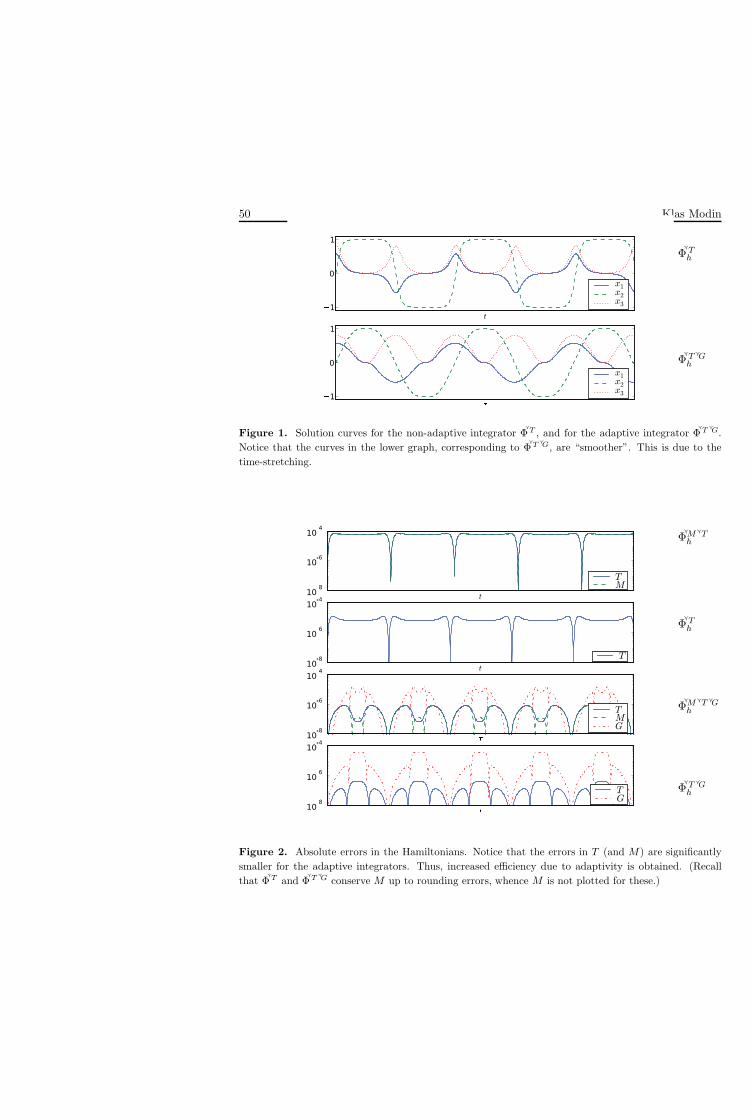
50 Klas Modin
Φ�Th
Φ�T �Gh
Figure 1. Solution curves for the non-adaptive integrator Φ�T , and for the adaptive integrator Φ
�T
�G.
Notice that the curves in the lower graph, corresponding to Φ�T
�G, are “smoother”. This is due to the
time-stretching.
Φ�M�Th
Φ�Th
Φ�M�T �Gh
Φ�T �Gh
Figure 2. Absolute errors in the Hamiltonians. Notice that the errors in T (and M) are significantlysmaller for the adaptive integrators. Thus, increased efficiency due to adaptivity is obtained. (Recallthat Φ
�T and Φ
�T
�G conserve M up to rounding errors, whence M is not plotted for these.)
Time transformation and reversibility of Nambu–Poisson systems 51
References
[1] D. Alekseevsky and P. Guha. On decomposability of Nambu-Poisson tensor. Acta Math. Univ.Comenian. (N.S.), 65 (19969, 1–9.
[2] S. Blanes and C. J. Budd. Adaptive geometric integrators for Hamiltonian problems with approxi-mate scale invariance. SIAM J. Sci. Comput., 26 (2005), 1089–1113 (electronic).
[3] S. D. Bond and B. J. Leimkuhler. Time-transformations for reversible variable stepsize integration.Numer. Algorithms, 19 (1998), 55–71,
[4] R. Chatterjee and L. Takhtajan. Aspects of classical and quantum Nambu mechanics. Lett. Math.Phys. 37 (1996), 475–482.
[5] S. Codriansky, R. Navarro, and M. Pedroza. The Liouville condition and Nambu mechanics. J.Phys. A, 29 (1996), 1037–1044.
[6] P. Gautheron. Some remarks concerning Nambu mechanics. Lett. Math. Phys. 37 (1996),103–116.[7] E. Hairer. Variable time step integration with symplectic methods. Appl. Numer. Math., 25 (1007),
219–227.[8] E. Hairer, C. Lubich, and G. Wanner. Geometric numerical integration. Springer Series in Compu-
tational Mathematics, 31, Springer-Verlag, Berlin, Second Ed., 2006.[9] E. Hairer and G. Soderlind. Explicit, time reversible, adaptive step size control. SIAM J. Sci.
Comput. 26 (2005), 1838–1851 (electronic).[10] W. Huang and B. Leimkuhler. The adaptive Verlet method. SIAM J. Sci. Comput. 18 (1997),
239–256.[11] R. Ibanez, M. de Leon, J. C. Marrero, and D. Martin de Diego. Dynamics of generalized Poisson
and Nambu-Poisson brackets. J. Math. Phys. 38 (1997), 2332–2344.[12] J. S. W. Lamb and J. A. G. Roberts. Time-reversal symmetry in dynamical systems: a survey. Phys.
D, 112 (1998), 1–39.[13] G. Marmo, G. Vilasi, and A. M. Vinogradov. The local structure of n-Poisson and n-Jacobi mani-
folds. J. Geom. Phys. 25 (1998), 141–182.[14] J. E. Marsden and T. S. Ratiu. Introduction to mechanics and symmetry, Texts in Applied Mathe-
matics, 17, Springer-Verlag, New York, Second Ed., 1999.[15] R. I. McLachlan. On the numerical integration of ordinary differential equations by symmetric
composition methods. SIAM J. Sci. Comput. 16 (1995),151–168.[16] R. I. McLachlan and G. R. W. Quispel. What kinds of dynamics are there? Lie pseudogroups,
dynamical systems and geometric integration. Nonlinearity, 14 (2001), 1689–1705.[17] R. I. McLachlan and G. R. W. Quispel. Splitting methods. Acta Numer. 11 (2002), 341–434, 2002.[18] S. Mikkola and P. Wiegert. Regularizing time transformations in symplectic and composite integra-
tion. Celestial Mech. Dynam. Astronom. 82 (2002), 375–390.[19] K. Modin. On explicit adaptive symplectic integration of separable Hamiltonian systems. Journal
of Multibody Dynamics, 2008 (to be published).[20] K. Modin and C. Fuhrer. Time-step adaptivity in variational integrators with application to contact
problems. ZAMM Z. Angew. Math. Mech. 86 (2006), 785–794.[21] P. Morando. Liouville condition, Nambu mechanics, and differential forms. J. Phys. A, 29 (1996),
L329–L331.[22] N. Nakanishi. On Nambu-Poisson manifolds. Rev. Math. Phys. 10 (1998), 499–510.[23] Y. Nambu. Generalized Hamiltonian dynamics. Phys. Rev. D, 7 (1973), 2405–2412.[24] M. Preto and S. Tremaine. A class of symplectic integrators with adaptive timestep for separable
hamiltonian systems. Astron. J. 118 (1999), 2532–2541.[25] R. Schmid. Infinite dimensional Lie groups with applications to mathematical physics. J. Geom.
Symmetry Phys. 1 (2004), 54–120.[26] D. Stoffer. Variable steps for reversible integration methods. Computing, 55 (1995), 1–22.

52 Klas Modin
[27] L. Takhtajan. On foundation of the generalized Nambu mechanics. Comm. Math. Phys. 160 (1994),295–315.
[28] I. Vaisman. A survey on Nambu-Poisson brackets. Acta Math. Univ. Comenian. (N.S.), 68 (1999),213–241.
[29] I. Vaisman. Nambu-Lie groups. J. Lie Theory, 10 (2000), 181–194.
Received September 10, 2008
Revised October 07, 2008

Paper V
Klas Modin, Dag Fritzson and Claus Führer.Proceedings of the 48th Scandinavian Conferenceon Simulation and Modeling (SIMS 2007).30-31 October, 2007, Göteborg (Särö), Sweden

Semiexplicit numerical integration bysplitting with application to dynamic
multibody problems with contactsKlas Modin and Dag Fritzson
SKF Engineering Research CentreMDC, RKs–2
SE–415 50 Göteborg, SwedenE–mail: [email protected], [email protected]
Claus FührerCentre for Mathematical SciencesBox 118, SE–221 00 Lund, Sweden
E–mail: [email protected]
October 7, 2008
Numerical integration is considered for second order differential equations on the form
q =A(q, q, t )+B(q, q, t ) ,
where A is significantly more expensive to evaluate than B , and B is stiff (highly oscillatory)in comparison with A. Examples of such problem are multibody problem with contactforces acting between bodies, and constraints formulated as penalty forces.
Based on the splitting A+B of the acceleration field, a numerical integration algorithm,which is explicit in the A–part and implicit in the B–part, is suggested. Consistency andlinear stability analysis of the proposed method is carried out.
Numerical examples with the proposed method is carried out for two simple test prob-lems, and for a complex multibody model of a rotating ball bearing. Comparison withconventional implicit methods is given for each example. The results indicate that theproposed method is more efficient, in terms of number of evaluations of A, at the sameaccuracy level.
1
Contents
Contents
1. Introduction 2
2. Characterization of the governing equations 22.1. Computational costs . . . . . . . . . . . . . . . . . . . . . . . . . . . . . . . . . . . . . . . . . . . . . 32.2. Estimated frequencies . . . . . . . . . . . . . . . . . . . . . . . . . . . . . . . . . . . . . . . . . . . . 4
3. Integrator algorithm 4
4. Consistency and linear stability analysis 54.1. Order of consistency . . . . . . . . . . . . . . . . . . . . . . . . . . . . . . . . . . . . . . . . . . . . 64.2. Stability analysis when B = 0 . . . . . . . . . . . . . . . . . . . . . . . . . . . . . . . . . . . . . . . 64.3. Full stability analysis . . . . . . . . . . . . . . . . . . . . . . . . . . . . . . . . . . . . . . . . . . . . 7
5. Adaptivity 105.1. Choice of control objective . . . . . . . . . . . . . . . . . . . . . . . . . . . . . . . . . . . . . . . . 10
6. Numerical examples 106.1. Harmonic oscillators . . . . . . . . . . . . . . . . . . . . . . . . . . . . . . . . . . . . . . . . . . . . 106.2. Non-linear pendulum . . . . . . . . . . . . . . . . . . . . . . . . . . . . . . . . . . . . . . . . . . . . 116.3. Complex ball bearing . . . . . . . . . . . . . . . . . . . . . . . . . . . . . . . . . . . . . . . . . . . . 11
7. Conclusions 15
References 17
1. Introduction
We are interested in the numerical time integration of dynamic multibody systems. In particular,problems where bodies frequently come in contact with each other, which is modelled by complexforce laws. The application we have in mind is simulation of rolling bearings, where contacts betweenbodies are present. Our aim is to design a numerical integrator that is particularly efficient for suchproblems.
In Section 2, a characterization of the governing equations is given. The objective is twofold: (i) topin-point where the computational cost is high; (ii) to estimate typical frequencies in the solution. Thespecific character of the governing equations is then used as a basis in Section 3 in order to design a moreefficient integrator. Further, in Section 4 the proposed integrator is analyzed in terms of consistencyand linear stability. In Section 5 we discuss issues concerned with adaptive time-stepping. Lastly, inSection 6, we give numerical test examples, both for simple test problems and for a fully complexrolling bearing problem.
2. Characterization of the governing equations
In this section we give an overview of the formulation, and a characterization, of the governing differ-ential equations that are to be numerically integrated. There are, of course, a number of choices on howto formulate the equations of motion for multibody systems. Primarily, the so called “floating frameof reference” is what we have in mind. In particular, the formulation used in the multibody simulationsoftware BEAST, which is a tool for detailed transient analysis of rolling bearings and other machine
2
2. Characterization of the governing equations
elements, developed and maintained by SKF (www.skf.com). For a full specification of the govern-ing equations, see [Nak06]. In this paper we consider only issues that are essential for the proposedintegrator.
Let Q = �d be the configuration space of the multibody system. Further, let q ∈ Q denote theposition coordinates. For rigid systems these are the centre of mass and the orientation of each body,relative to a fixed global coordinate system in Euclidean 3–space. In the case of elasiticity, generalizedcoordinates describing the deflection field of each body are also included in q. The governing equationsare on the form
M (q, q)q = F (q, q, t ) , q(0) = q0 , q(0) = q0 , (1)
where the mass matrix M (q, q) is a symmetric positive definite d × d–matrix, and the force fieldF (q, q, t ) is a vector valued map corresponding to the forces acting on the system. Time is denoted t .Notice that (1) is a second order ordinary differential equation (ODE).
Constraints are taken into account by penalty force laws. Thus, we do not utilize the standardLagrangian multiplier formulation, which is typically used for constrained mechanical systems. Noticethat the penalty formulation implies that (1) is highly stiff. Thus, an implicit numerical integrator mustbe used.
Remark. The integrator suggested in this paper could easily be extended to governing equations formu-lated as a differential algebraic system using Lagrangian multipliers.
2.1. Computational costs
Solving (1) numerically with a standard ODE solver basically involves the following computations inorder to evaluate the vector field:
• Compute the inverse of the mass matrix. This is a cheap operation, as the mass matrix is blockdiagonal (one block per body).
• Compute the constraint forces, which is also cheap.
• Compute “simple” non-stiff forces such as gravity and Coriolis forces.
• Compute contact forces. This task is heavily dominating the computational cost. Evaluationof each contact involves searching for intersecting surfaces. In the case of rolling bearings, thesurface geometries of the bodies are highly complex. Further, for very detailed contact models(as in BEAST), tribological issues, such as oil film thickness in the contact, are also taken intoaccount. See [SF01] for details on advanced contact modelling.
In order to be able to separate the computationally intensive force evaluations from less costly evalua-tions, we rewrite (1) as
M (q, q)q = F A(q, q, t )+ F B (q, q, t ) , (2)
where F A are the contact forces plus “simple” non-stiff forces (from now on we refer to F A as contactforces), and F B are the constraint penalty forces. Multiplying from the left with the inverse of the massmatrix we get a second order ODE written on standard form
q =A(q, q, t )+B(q, q, t ) or shorter q =C (q, q, t ) . (3)
The maps A and B correspond to accelerations due to contact forces and constraint forces respectively.C = A+ B is the total acceleration field. The field A is much more expensive to compute than B .This “splitting formulation” of the governing equations will be utilized by the integrator algorithmdescribed in Section 3.
3
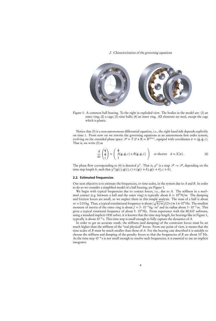
2. Characterization of the governing equations
Figure 1: A common ball bearing. To the right in exploded view. The bodies in the model are: (1) anouter ring; (2) a cage; (3) nine balls; (4) an inner ring. All elements are steel, except the cagewhich is plastic.
Notice that (3) is a non-autonomous differential equation, i.e., the right hand side depends explicitlyon time t . From now on we rewrite the governing equations as an autonomous first order system,evolving on the extended phase space P = T Q� = �2d+1, equiped with coordinates z = (q, q, t ).That is, we write (3) as
d
dt
⎛⎜⎝qqt
⎞⎟⎠=⎛⎜⎝ q
A(q, q, t )+B(q, q, t )1
⎞⎟⎠ or shorter z =X (z ) . (4)
The phase flow corresponding to (4) is denoted ϕh . That is, ϕh is a map P →P , depending on thetime step length h, such that ϕh (q(t ), q(t ), t ) = (q(t + h), q(t + h), t + h).
2.2. Estimated frequencies
Our next objective is to estimate the frequencies, or time scales, in the system due to A and B . In orderto do so we consider a simplified model of a ball bearing, see Figure 1.
We begin with typical frequencies due to contact forces, i.e., due to A. The stiffness in a steel–steel contact (e.g. between a ball and the outer ring) is typically about k = 108 N/m. The dampingand friction forces are small, so we neglect them in this simple analysis. The mass of a ball is aboutm = 0.01kg. Thus, a typical translational frequency is about (
k/m)/(2π)≈ 1.6·104 Hz. The smallest
moment of inertia of the outer ring is about J = 3 · 10−5 kg ·m2 and its radius about 3 · 10−2 m. Thisgives a typical rotational frequency of about 5 · 104 Hz. From experience with the BEAST software,using a standard implicit ODE solver, it is known that the time step length, for bearings like in Figure 1,typically is about 10−6 s. This time step is small enough to fully capture the dynamics of A.
In order to get an accurate result, the stiffness (and damping) of the constraint forces must be setmuch higher than the stiffness of the “real physical” forces. From our point of view, it means that thetime scales of B must be much smaller than those of A. For the bearing case described it is suitable tochoose the stiffness and damping of the penalty forces so that the frequencies of B are about 107 Hz.As the time step 10−6 s is not small enough to resolve such frequencies, it is essential to use an implicitintegrator.
4
3. Integrator algorithm
3. Integrator algorithm
From the previous section it is clear that the governing equations are stiff due to constraint forces, so forthe time step lengths we have in mind an implicit integrator is needed in order to achieve stability. Froman efficiency point of view, an implicit integrator is, per time step, more expensive than an explicit dito,because at each step a non–linear root finding problem needs to be solved iteratively. In particular, thisimplies that A and B are evaluated several times per time step. Furthermore, the Jacobian needs to becomputed for an implicit method (which is severely expensive for A in our case), as it is used by theroot finding algorithm (typically some variant of Newton’s method).
The frequency analysis of the previous section indicates that the dynamics of A can be resolvedaccuratelly with an explicit integrator for the time step lengths we have in mind. However, it is not sofor B . One possibility is of course to choose a much smaller time step, but that would be inefficient, asto many time steps are needed.
Our approach is to treat A explicitly and B implicitly. The notion is that B is “responsible” for thestiff character of the system, so in order to have stability for long time steps it is enough if only thispart is handled implicitly. The idea is that the number of evaluations of A should be on par with thatof explicit methods, whereas B can be evaluted more frequently without any significant increase in thecomputational cost.
An obvious possibility is to use so called splitting methods (see [MQ02]). That is, to consider anexplicit method ΦA
hfor the equation q = A(q, q, t ) and an implicit method ΦB
h for q = B(q, q, t ), andthen utilized a composition of the two methods, e.g. ΦA
h◦ΦB
h or ΦBh/2◦ΦA
h◦ΦB
h/2. However, this approach
is not so good in our case. Indeed, asΦAh
does not take constraint forces into account, the solution wouldat each step drift away a little from the constraint manifold, and then be “forced back” towards it by ΦB
h .As ΦB
h does not exactly project onto the constraint manifold, high frequency O(h) oscillations wouldthus appear in the solution.
We suggest the following discretization of the governing equations (4)
qn+1 = qn + h qn +h2
2
�An+α+Bn+β
�qn+1 = qn + h
�An+α+Bn+β
�tn+1 = tn + h ,
(5)
where α,β ∈ [0,1] are method parameters and
An+α =A(qn + hαqn , qn , tn +αh)
Bn+β = B�(1−β)z n +βz n+1
�, z n = (qn , qn , tn) .
Notice that An+α is independent of qn+1 and qn+1 for all α. Thus, it only needs to be evaluated onceper time step, and the Jacobian of A is not needed. This is what we mean by “treating A explicitly”.
The method (5) is a blend of the Störmer–Verlet method, the explicit Euler method, and the implicitmidpoint rule. The correspondence is as follows.
Condition Method
B = 0, α= 1/2, and A independent of q Störmer–VerletB = 0 and A independent of q explicit Euler (for the q part)A= 0 and β= 1/2 implicit midpoint rule
5
4. Consistency and linear stability analysis
4. Consistency and linear stability analysis
In this section we analyse the order of consistency and the linear stability of the proposed method (5).We begin with the consistency analysis. Next, the stability analysis, which is split into two parts. Firstthe explicit component of the algorithm is analysed separately, i.e. the case B = 0. Based on theseresults, stability of the full algorithm, with constraint forces present, is thereafter analysed.
4.1. Order of consistency
Let Φh : P→P be the numerical flow of (5), i.e., the map defined by
Φh (qn , qn , tn) = (qn+1, qn+1, tn+1) .
The local error map is given by Eh = Φh − ϕh . Consistency of Φh with respect to ϕh means thatEh (z ) =O(h2) as h→ 0 for all z ∈P . Concering the principle term of Eh we have the following result:
Lemma 1. The q , q and t components of the local error map Eh fulfills
Eh (z ) =
⎛⎜⎜⎜⎝16 h3
�(3α− 1)
�∂qA(z )q + ∂t A(z )
�− ∂qA(z )C (z )+ (3β− 1)∂z B(z )X (z )�+O(h4)
12 h2
�(2α− 1)
�∂qA(z )q + ∂t A(z )
�− ∂qA(z )C (z )+ (2β− 1)∂z B(z )X (z )�+O(h3)
0
⎞⎟⎟⎟⎠ .
Proof. Compare Taylor expansions in h of Φh (z ) and ϕh (z ).
Using the lemma we immediatelly obtain the following result:
Theorem 2. The method Φh , defined by (5), has the following order of consistency properties.
• It is consistent for all α,β.
• It is second order accurate in position variables q for all α,β.
• If α=β= 1/2 and A is independent of q , then it is second order accurate in all variables.
Remark. In our application, the friction and damping in the contacts are very small in comparison tothe stiffness. That is, ‖∂qA(z )‖ is small in comparison to ‖∂qA(z )‖. Thus, we have “almost” secondorder accuracy for α=β= 1/2.
4.2. Stability analysis when B = 0
In absence of constraint forces, i.e., when B = 0, the method Φh is fully explicit. Thus, it has a boundedstability region in terms of the step size h. We carry out a linear stability analysis for the scalar testequation given by
q =A(q , q) =−kq − c q , k , c ∈� . (6)
Recall that stability of the method Φh means that limn→∞Φnh(z ) is bounded. The result is as follows.
Theorem 3. The stability region of the method (5) applied to (6) (with B = 0) is given by
Ω= (hc , h2k) ∈�2 \ {(0,0), (2− 4α, 4)} ; h2k ≥ 0, hc ≤ 2−αh2k , hc ≥ (1/2−α)h2k
!. (7)
See Figure 2 for an illustration.
6
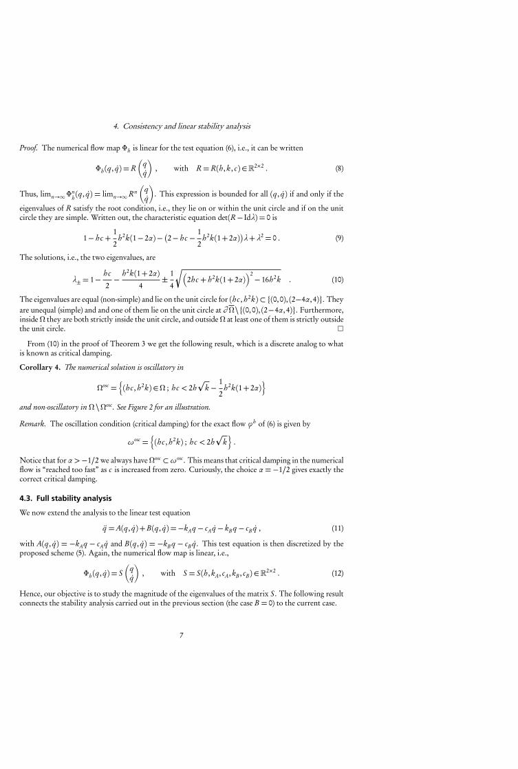
4. Consistency and linear stability analysis
Proof. The numerical flow map Φh is linear for the test equation (6), i.e., it can be written
Φh (q , q) = R�
�, with R= R(h, k , c) ∈�2×2 . (8)
Thus, limn→∞Φnh(q , q) = limn→∞Rn
�. This expression is bounded for all (q , q) if and only if the
eigenvalues of R satisfy the root condition, i.e., they lie on or within the unit circle and if on the unitcircle they are simple. Written out, the characteristic equation det(R− Idλ) = 0 is
1− hc +1
2h2k(1− 2α)− �2− hc − 1
2h2k(1+ 2α)
�λ+λ2 = 0 . (9)
The solutions, i.e., the two eigenvalues, are
λ± = 1− hc
2− h2k(1+ 2α)
4± 1
4
"�2hc + h2k(1+ 2α)
�2− 16h2k . (10)
The eigenvalues are equal (non-simple) and lie on the unit circle for (hc , h2k)⊂ {(0,0), (2−4α, 4)}. Theyare unequal (simple) and and one of them lie on the unit circle at ∂ Ω\{(0,0), (2−4α, 4)}. Furthermore,inside Ω they are both strictly inside the unit circle, and outside Ω at least one of them is strictly outsidethe unit circle.
From (10) in the proof of Theorem 3 we get the following result, which is a discrete analog to whatis known as critical damping.
Corollary 4. The numerical solution is oscillatory in
Ωosc = (hc , h2k) ∈Ω ; hc < 2h
k − 1
2h2k(1+ 2α)
!and non-oscillatory in Ω \Ωosc. See Figure 2 for an illustration.
Remark. The oscillation condition (critical damping) for the exact flow ϕh of (6) is given by
ωosc = (hc , h2k) ; hc < 2h
k!
.
Notice that for α >−1/2 we always haveΩosc ⊂ωosc. This means that critical damping in the numericalflow is “reached too fast” as c is increased from zero. Curiously, the choice α =−1/2 gives exactly thecorrect critical damping.
4.3. Full stability analysis
We now extend the analysis to the linear test equation
q =A(q , q)+B(q , q) =−kAq − cAq − kB q − cB q , (11)
with A(q , q) = −kAq − cAq and B(q , q) = −kB q − cB q . This test equation is then discretized by theproposed scheme (5). Again, the numerical flow map is linear, i.e.,
Φh (q , q) = S�
�, with S = S(h, kA, cA, kB , cB ) ∈�2×2 . (12)
Hence, our objective is to study the magnitude of the eigenvalues of the matrix S. The following resultconnects the stability analysis carried out in the previous section (the case B = 0) to the current case.
7
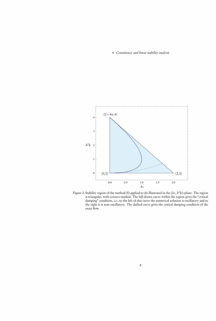
4. Consistency and linear stability analysis
0.0 0.5 1.0 1.5 2.0
0
1
2
3
4
hc
h2k
(0,0)
(2− 4α, 4)
(2,0)
Figure 2: Stability region of the method (5) applied to (6) illustrated in the (hc , h2k)–plane. The regionis triangular, with corners marked. The full drawn curve within the region gives the “criticaldamping” condition, i.e., to the left of this curve the numerical solution is oscillatory and tothe right it is non–oscillatory. The dashed curve gives the critical damping condition of theexact flow.
8
4. Consistency and linear stability analysis
Lemma 5. The transformation
hc ←→ 2h(cA+ cB )
2+ 2βhcB +βh2kB
(13a)
h2k ←→ 2h2(kA+ kB )
2+ 2βhcB +βh2kB
(13b)
α ←→ αh2kA+βh2kB
h2kA+ h2kB
(13c)
takes the characteristic equation (9) into the characteristic equation det(S − Idλ) = 0.
Proof. Substitute (hc , h2k ,α) in (9) by the transformation (13). The resulting equation coincides withthe characteristic equation det(S − Idλ) = 0.
From Theorem 3 we know for which (hc , h2k ,α) the eigenvalues of R in (8) fulfill the root condition.Thus, using Lemma 5, we can investigate the root condition for the eigenvalues of S in (12). Thefollowing result, which asserts that the stability of the “explicit part” is not affected by the “implicitpart”, is then obtained:
Theorem 6. For β≥ 1/2 the method (5) applied to (11) is stable for all kB , cB ≥ 0 if (hcA, h2kA) ∈Ω.
Proof. From Theorem 3 it follows that the root condition is fulfilled for the roots of (9) if
(i) h2k ≥ 0 ,
(ii) hc +αh2k ≤ 2 ,
(iii) (1/2−α)h2k − hc ≤ 0 .
Using Lemma 5, the root condition for the roots of det(S − Idλ) = 0 are fulfilled if the conditionsobtained by substituting (13) in (i)–(iii) are fulfilled. Thus, our objective is to investigate (i)–(iii) afterthe substitution (13).
(i) Trivial because (13b) is always non-negative, so the condition is always true.(ii) After substitution the condition becomes
2hcA+ 2αh2kA+ 2hcB + 2βh2kB
2+ 2βhcB +βh2kB
≤ 2 .
For β ≥ 1/2 the left hand side is a decreasing function of both cB and kB . Thus, the left hand side ismaximal when cB = kB = 0, which corresponds to the case B = 0.
(iii) After substitution the condition becomes
h2kA(1− 2α)− 2hcA+ h2kB (1− 2β)− 2hcB
2+ 2βhcB +βh2kB
≤ 0 .
Again, for β ≥ 1/2 the left hand side is a decreasing function of both cB and kB , and the maximumat cB = kB = 0 corresponds to the case B = 0.
Remark. The stability result in Theorem 6 is the best possible, because for B = 0 it replicates Theo-rem 3, and for A= 0 it gives unconditional stability (cooresponding exactly to the classical θ–methodwith θ=β).
9
5. Adaptivity
5. Adaptivity
In order to increase the efficiency of the integration process it is important to introduce adaptive timestepping. There are various ways of doing this. It is out of scope of this paper to discuss any of them infull detail, but we mention two techniques.
The classical approach is to estimate the local error l err at each time step, and then to consider thecontrol objective l err ≈ tol for some user specified tolerance level tol, see [Söd02, Söd03] for details.
Another approach, which is typically used in conjunction with geometric integration, is to introducea Sundman transformation of the governing equations, which is a dynamic time transformation. Let sbe a strictly positive real valued function on the phase space P , called a scaling function, and introducea new independent variable τ defined dynamically by d/dτ = s (z )d/dt . The governing equations (4)then transform into
dz
dτ= s (z )X (z ) . (14)
Solutions to (14) correspond to time stretched solutions of (4). Thus, equidistant steps ε in the τ–domaincorrespond to variable steps h = h(z ) = s (z )ε in the physical time domain. The easiest way to use thisapproach in conjunction with the proposed method (5) is to set h = s (z n)ε at each step n→ n+ 1. Forother, more intricate, techniques that also conserve the geometric properties of the flow (e.g. energyfor conservative systems), see [MF06, HS05, HLW06].
5.1. Choice of control objective
As mentioned above, in classical ODE solvers the local error is estimated at each time step and is usedas step size control objective. We suggest another choice based instead on the stability condition.
In Section 4 we found that for A only dependent on q and t (i.e. no damping), the linear stabilitycondition is h2σ(∂ A(z )/∂ q)≤ 4. Thus, if an estimate σ est ≈ σ(∂qA(z )) is available, then a feasible stepsize control objective is h2σ est ≈ tol ≤ 4.
For the proposed algorithm (5), an estimate of hα∂qA(z n)q is given by An+α−An . Thus, the quantity
σ est =‖An+α−An‖
hα‖q‖ (15)
gives an estimate of the stiffness in the direction of the flow. Notice that (15) is a function of z n , i.e.,σ est = σ est(z ) is a function on the phase space P . Thus, the corresponding scaling function is givenby s (z ) = 1/
σ est(z ). Hence, the Sundman transformation technique (14) may be used in conjunction
with this control objective. Furthermore, from Lemma 1 it is evident that for α �= 1/2 this choicecorresponds to keeping the principle relative local error term constant for velocity variables.
6. Numerical examples
In this section we present numerical examples of the proposed algorithm (5) applied to: (1) a simplelinear problem consisting of two harmonic oscillators; (2) a non-linear pendulum problem in Cartesiancoordinates; and (3) a complex multibody ball bearing problem. The last example is carried out in themultibody environment BEAST, where the method has been implemented.
6.1. Harmonic oscillators
The problem describes two particles, both with mass 1, moving on the real line. Between the twoparticles there is a linear spring with stiffness 103 and damping 102. One of the particles is attached to
10
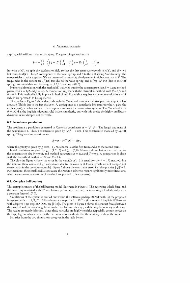
6. Numerical examples
a spring with stiffness 1 and no damping. The governing equations are
q =−�
1 00 0
�q − 103
�1 −1−1 1
�q − 102
�1 −1−1 1
�q .
In terms of (3), we split the acceleration field so that the first term corresponds to A(z ), and the twolast terms to B(z ). Thus, A corresponds to the weak spring, and B to the stiff spring “constraining” thetwo particles to stick together. We are interested in resolving the dynamics in A, but not that in B . Thefrequencies in the system are 1/(4π) Hz (due to the weak spring) and (1/π) · 103 Hz (due to the stiffspring). As initial data we choose q0 = (1.0,1.1) and q0 = (0,0).
Numerical simulation with the method (5) is carried out for the constant step size h = 1, and methodparameters α= 1/2 andβ= 0.8. A comparison is given with the classical θ–method, with θ= 1/2 andθ = 0.8. This method is fully implicit in both A and B , and thus requires many more evaluations of A(which we “pretend” to be expensive).
The results in Figure 3 show that, although the θ–method is more expensive per time step, it is lessaccurate. This is due to the fact that α= 1/2 corresponds to a symplectic integrator for the A–part (theexplicit part), which is known to have superior accuracy for conservative systems. The θ–method withθ = 1/2 (i.e. the implicit midpoint rule) is also symplectic, but with this choice the highly oscillatorydynamics is not damped out correctly.
6.2. Non-linear pendulum
The problem is a pendulum expressed in Cartesian coordinates q = (q x , qy ). The length and mass ofthe pendulum is 1. Thus, a constraint is given by ‖q‖2 − 1 = 0. This constraint is modeled by as stiffspring. The governing equations are
q = g − 104(‖q‖2− 1)q ,
where the gravity is given by g = (0,−1). We choose A as the first term and B as the second term.Initial conditions are given by q0 = (1.01,0) and q0 = (0,0). Numerical simulation is carried out for
the constant step size h = 0.01, and method parameters α = 1/2 and β = 0.6. A comparison is givenwith the θ–method, with θ= 1/2 and θ= 0.6.
The plots in Figure 4 show the error in the variable q x . It is small for the θ = 1/2 method, butthe solution there contains high oscillations due to the constraint forces, which are not damped outcorrectly (as in the previous example). Figure 5 shows the constraint error, i.e., the quantity ‖q‖2− 1.Furthermore, these small oscillations cause the Newton solver to require significantly more iterations,which means more evaluations of A (which we pretend to be expensive).
6.3. Complex ball bearing
This example consists of the ball bearing model illustrated in Figure 1. The outer ring is held fixed, andthe inner ring is rotated with 104 revolutions per minute. Further, the inner ring is loaded axially witha constant force of 103 N.
Simulations of the system is carried out within the software package BEAST with: (i) the proposedintegrator with α = 1/2, β = 0.8 and constant step size h = 10−6 s; (ii) a standard implicit BDF–solverwith adaptive time steps (CVODE, see [Hin]). The plots in Figure 6 show: the contact forces betweenthe first ball and the outer ring; between the first ball and the cage; and the angular velocity of the cage.The results are nearly identical. Since these variables are highly sensitive (especially contact forces onthe cage) high similarity between the two simulations indicate that the accuracy is about the same.
Statistics from the two simulations are given in the table below.
11
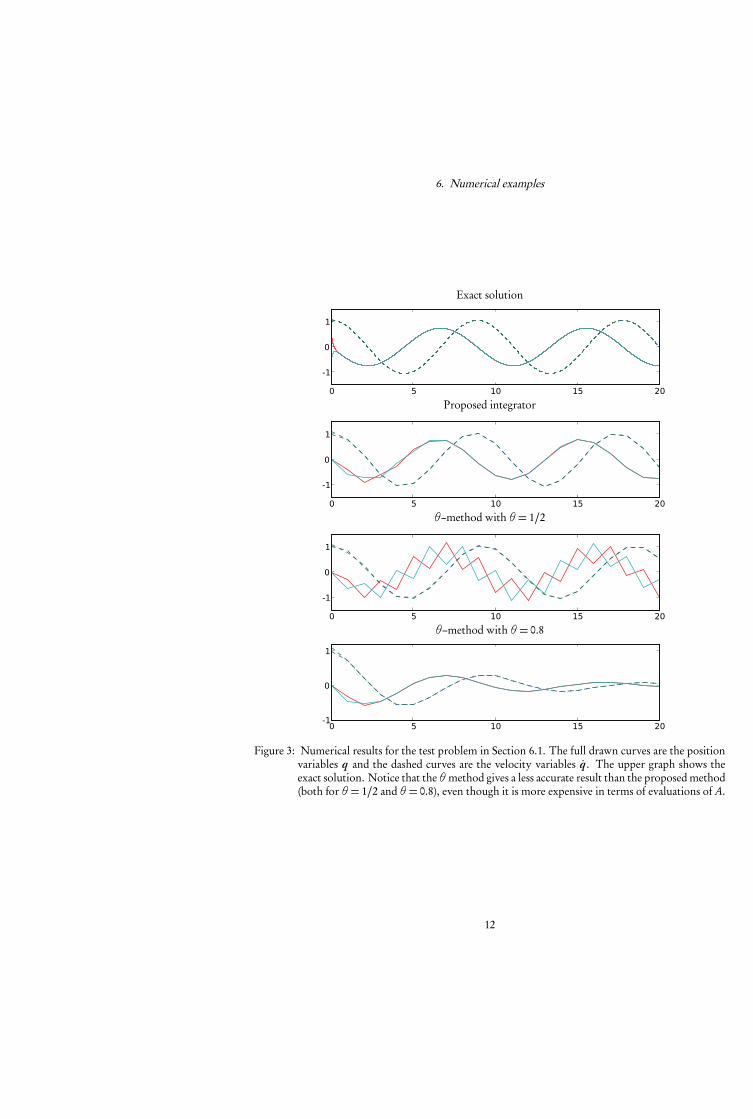
6. Numerical examples
Exact solution
0 5 10 15 20
-1
0
1
Proposed integrator
0 5 10 15 20
-1
0
1
θ–method with θ= 1/2
0 5 10 15 20
-1
0
1
θ–method with θ= 0.8
0 5 10 15 20-1
0
1
Figure 3: Numerical results for the test problem in Section 6.1. The full drawn curves are the positionvariables q and the dashed curves are the velocity variables q. The upper graph shows theexact solution. Notice that the θmethod gives a less accurate result than the proposed method(both for θ= 1/2 and θ= 0.8), even though it is more expensive in terms of evaluations of A.
12
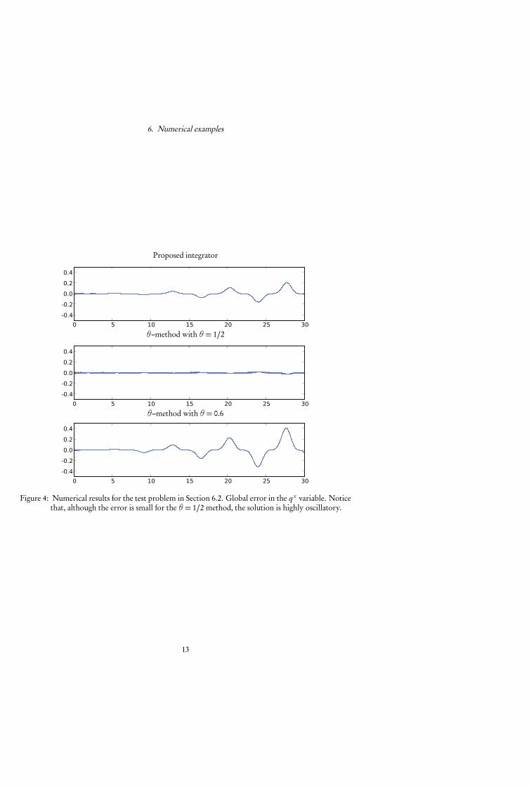
6. Numerical examples
Proposed integrator
0 5 10 15 20 25 30
-0.4
-0.2
0.0
0.2
0.4
θ–method with θ= 1/2
0 5 10 15 20 25 30
-0.4
-0.2
0.0
0.2
0.4
θ–method with θ= 0.6
0 5 10 15 20 25 30
-0.4
-0.2
0.0
0.2
0.4
Figure 4: Numerical results for the test problem in Section 6.2. Global error in the q x variable. Noticethat, although the error is small for the θ= 1/2 method, the solution is highly oscillatory.
13
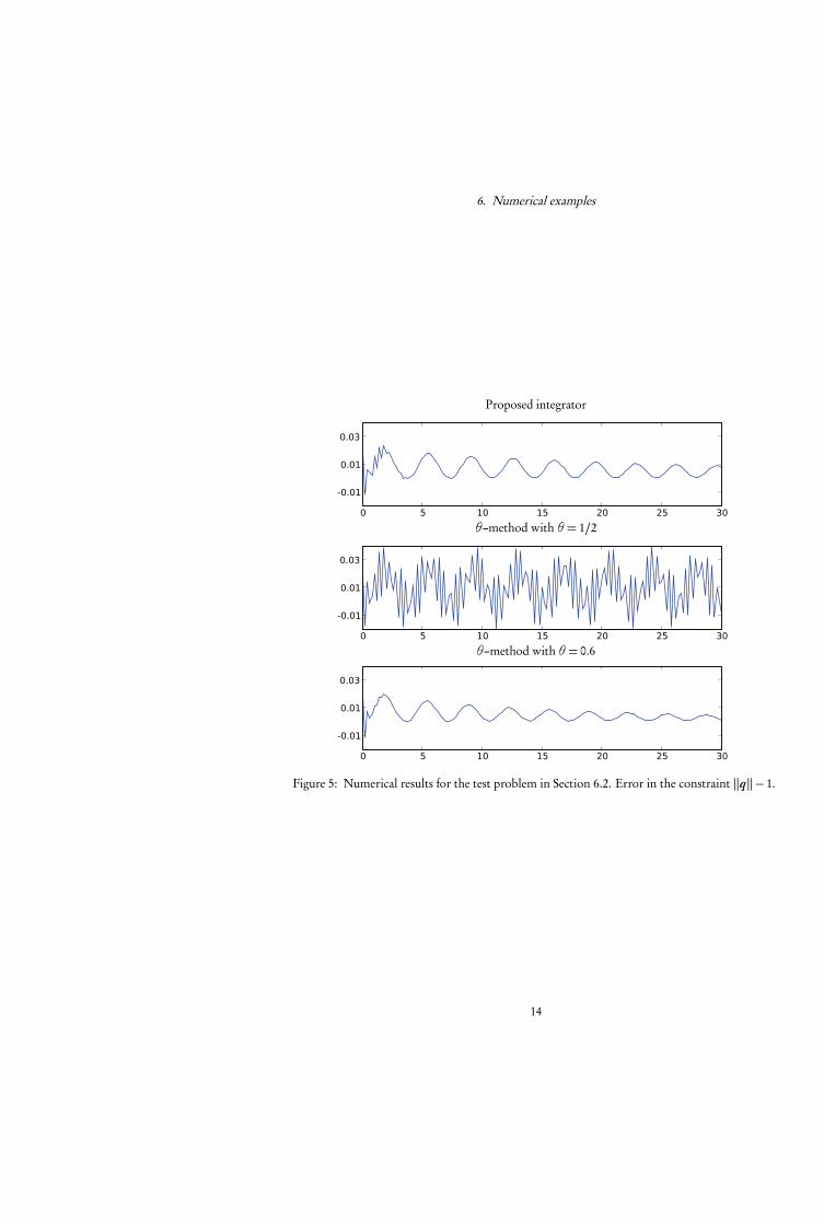
6. Numerical examples
Proposed integrator
0 5 10 15 20 25 30
-0.01
0.01
0.03
θ–method with θ= 1/2
0 5 10 15 20 25 30
-0.01
0.01
0.03
θ–method with θ= 0.6
0 5 10 15 20 25 30
-0.01
0.01
0.03
Figure 5: Numerical results for the test problem in Section 6.2. Error in the constraint ‖q‖− 1.
14
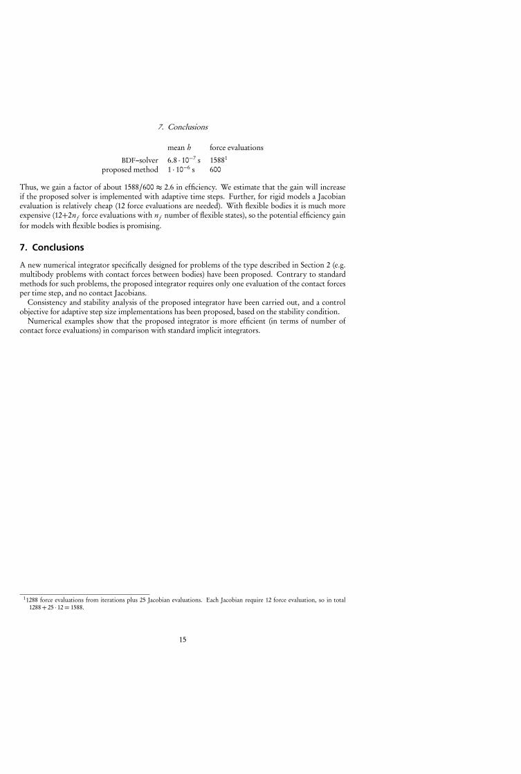
7. Conclusions
mean h force evaluations
BDF–solver 6.8 · 10−7 s 15881
proposed method 1 · 10−6 s 600
Thus, we gain a factor of about 1588/600 ≈ 2.6 in efficiency. We estimate that the gain will increaseif the proposed solver is implemented with adaptive time steps. Further, for rigid models a Jacobianevaluation is relatively cheap (12 force evaluations are needed). With flexible bodies it is much moreexpensive (12+2nf force evaluations with nf number of flexible states), so the potential efficiency gainfor models with flexible bodies is promising.
7. Conclusions
A new numerical integrator specifically designed for problems of the type described in Section 2 (e.g.multibody problems with contact forces between bodies) have been proposed. Contrary to standardmethods for such problems, the proposed integrator requires only one evaluation of the contact forcesper time step, and no contact Jacobians.
Consistency and stability analysis of the proposed integrator have been carried out, and a controlobjective for adaptive step size implementations has been proposed, based on the stability condition.
Numerical examples show that the proposed integrator is more efficient (in terms of number ofcontact force evaluations) in comparison with standard implicit integrators.
11288 force evaluations from iterations plus 25 Jacobian evaluations. Each Jacobian require 12 force evaluation, so in total1288+ 25 · 12= 1588.
15
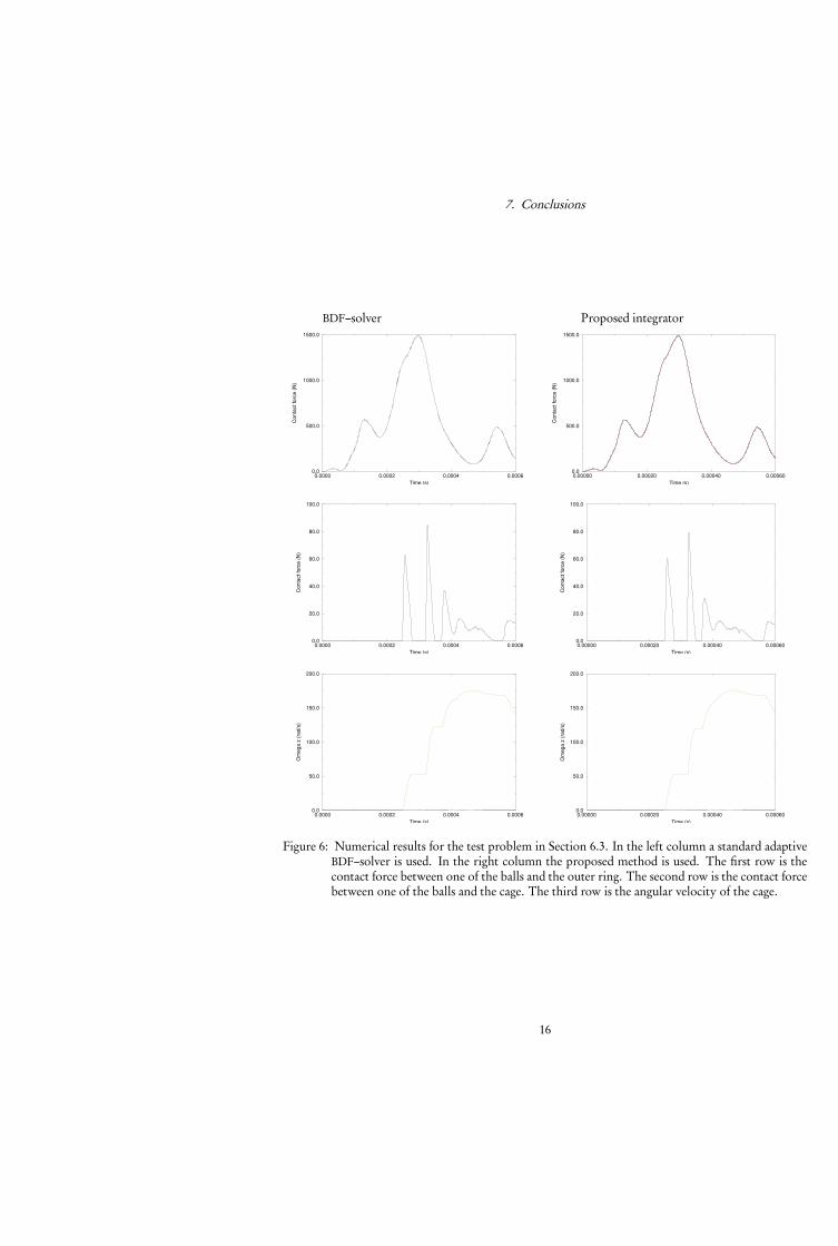
7. Conclusions
BDF–solver Proposed integrator
0.0000 0.0002 0.0004 0.0006Time (s)
0.0
500.0
1000.0
1500.0
Con
tact
forc
e (N
)
0.00000 0.00020 0.00040 0.00060Time (s)
0.0
500.0
1000.0
1500.0
Con
tact
forc
e (N
)
0.0000 0.0002 0.0004 0.0006Time (s)
0.0
20.0
40.0
60.0
80.0
100.0
Con
tact
forc
e (N
)
0.00000 0.00020 0.00040 0.00060Time (s)
0.0
20.0
40.0
60.0
80.0
100.0
Con
tact
forc
e (N
)
0.0000 0.0002 0.0004 0.0006Time (s)
0.0
50.0
100.0
150.0
200.0
Om
ega
z (r
ad/s
)
0.00000 0.00020 0.00040 0.00060Time (s)
0.0
50.0
100.0
150.0
200.0
Om
ega
z (r
ad/s
)
Figure 6: Numerical results for the test problem in Section 6.3. In the left column a standard adaptiveBDF–solver is used. In the right column the proposed method is used. The first row is thecontact force between one of the balls and the outer ring. The second row is the contact forcebetween one of the balls and the cage. The third row is the angular velocity of the cage.
16
References
References
[Hin] A. Hindmarsh. CVODE open-source software. www.llnl.gov/CASC/sundials/.
[HLW06] Ernst Hairer, Christian Lubich, and Gerhard Wanner. Geometric numerical integration,volume 31 of Springer Series in Computational Mathematics. Springer-Verlag, Berlin, secondedition, 2006. Structure-preserving algorithms for ordinary differential equations.
[HS05] Ernst Hairer and Gustaf Söderlind. Explicit, time reversible, adaptive step size control.SIAM J. Sci. Comput., 26(6):1838–1851 (electronic), 2005.
[MF06] Klas Modin and Claus Führer. Time-step adaptivity in variational integrators with applica-tion to contact problems. ZAMM Z. Angew. Math. Mech., 86(10):785–794, 2006.
[MQ02] Robert I. McLachlan and G. Reinout W. Quispel. Splitting methods. Acta Numer., 11:341–434, 2002.
[Nak06] I. Nakhimovski. Contributions to the Modeling and Simulation of Mechanical Systems withDetailed Contact Analyses. PhD thesis, LinkÃupings Universitet, LinkÃuping, 2006.
[SF01] L-E Stacke and D. Fritzson. Dynamical behaviour of rolling bearings: simulations andexperiments. Proc. Instn. Mech. Engrs., 215:499–508, 2001.
[Söd02] Gustaf Söderlind. Automatic control and adaptive time-stepping. Numer. Algorithms, 31(1-4):281–310, 2002. Numerical methods for ordinary differential equations (Auckland, 2001).
[Söd03] Gustaf Söderlind. Digital filters in adaptive time-stepping. ACM Trans. Math. Software,29(1):1–26, 2003.
17


![Adaptive Geometric Numerical Integration of Mechanical ...lup.lub.lu.se/search/ws/files/4144628/1390977.pdf · of Ordinary Differential Equations” [13]. Since then Dahlquist’s](https://static.fdocuments.net/doc/165x107/5f3f654d87f71d6a2f1474e2/adaptive-geometric-numerical-integration-of-mechanical-luplublusesearchwsfiles4144628.jpg)