Adaptive interpretation of gas well deliverability tests · Adaptive interpretation of gas well ......
6
Adaptive interpretation of gas well deliverability tests V L Sergeev, Nguyen Thac Hoai Phuong and A B Strelnikova National Research Tomsk Polytechnic University, 30 Lenina Ave., Tomsk, 634050, Russia [email protected], [email protected] Abstract. The paper considers topical issues of improving accuracy of data obtained from gas well deliverability tests, decreasing the number of test stages and well test time, and reducing gas emissions. The aim of the research is to develop the method of adaptive interpretation of gas well deliverability tests with resulting IPR curve conducted in gas wells with steady-state filtration, which allows obtaining and taking into account additional a priori data on the formation pressure and flow coefficients, setting the number of test stages adequate for efficient well testing and reducing test time. The present research is based on the previous theoretical and practical findings in the spheres of gas well deliverability tests, systems analysis, system identification, function optimization and linear algebra. To test the method, the authors used the field data of deliverability tests run in the Urengoy gas and condensate field, Tyumen Oblast. The authors suggest the method of adaptive interpretation of gas well deliverability tests with resulting IPR curve, which is based on the law for gas filtration with variables dependent on the number of test stage and account of additional a priori data. The suggested method allows defining the estimates of the formation pressure and flow coefficients, optimal in terms of preassigned measures of quality, and setting the adequate number of test stages in the course of well testing. The case study of IPR curve data processing has indicated that adaptive interpretation provides more accurate estimates on the formation pressure and flow coefficients, as well as reduces the number of test stages. 1. Introduction Deliverability tests with resulting inflow performance relationship (IPR) curve run in the gas wells with steady-state filtration are one of the most informative and common methods well tests to characterize the behavior of well and the bottomhole conditions. Currently, the data obtained via deliverability tests are interpreted using the methods described in [1-3], which are based on Forchheimer binomial equation for gas filtration: 2 2 2 пл з p p aq bq , (1) where 2 2 , пл з p p are formation pressure and bottomhole pressure, respectively; a and b- flow coefficients dependent on bottomhole zone parameters and bottomhole structure; q - flow rate. The coefficients a and b for IPR curve model (1) should be estimated using least square method, with the formation pressure being known [2-4]. IPR interpretation based on the model (1) and least square method is challengeable as a field method, which is attributed to the following facts: the formation pressure is difficult to determine, estimates should be robust and accurate, the number of test stages (a number of “cycles” characterized by a stabilized flow when the pressure and flow rate are recorded) is reduced. PGON2016 IOP Publishing IOP Conf. Series: Earth and Environmental Science 43 (2016) 012015 doi:10.1088/1755-1315/43/1/012015 Content from this work may be used under the terms of the Creative Commons Attribution 3.0 licence. Any further distribution of this work must maintain attribution to the author(s) and the title of the work, journal citation and DOI. Published under licence by IOP Publishing Ltd 1
Transcript of Adaptive interpretation of gas well deliverability tests · Adaptive interpretation of gas well ......
Adaptive interpretation of gas well deliverability tests
V L Sergeev, Nguyen Thac Hoai Phuong and A B Strelnikova
National Research Tomsk Polytechnic University, 30 Lenina Ave., Tomsk, 634050,
Russia
[email protected], [email protected]
Abstract. The paper considers topical issues of improving accuracy of data obtained from gas
well deliverability tests, decreasing the number of test stages and well test time, and reducing
gas emissions. The aim of the research is to develop the method of adaptive interpretation of
gas well deliverability tests with resulting IPR curve conducted in gas wells with steady-state
filtration, which allows obtaining and taking into account additional a priori data on the
formation pressure and flow coefficients, setting the number of test stages adequate for
efficient well testing and reducing test time. The present research is based on the previous
theoretical and practical findings in the spheres of gas well deliverability tests, systems
analysis, system identification, function optimization and linear algebra. To test the method,
the authors used the field data of deliverability tests run in the Urengoy gas and condensate
field, Tyumen Oblast. The authors suggest the method of adaptive interpretation of gas well
deliverability tests with resulting IPR curve, which is based on the law for gas filtration with
variables dependent on the number of test stage and account of additional a priori data. The
suggested method allows defining the estimates of the formation pressure and flow
coefficients, optimal in terms of preassigned measures of quality, and setting the adequate
number of test stages in the course of well testing. The case study of IPR curve data
processing has indicated that adaptive interpretation provides more accurate estimates on the
formation pressure and flow coefficients, as well as reduces the number of test stages.
1. Introduction
Deliverability tests with resulting inflow performance relationship (IPR) curve run in the gas wells
with steady-state filtration are one of the most informative and common methods well tests to
characterize the behavior of well and the bottomhole conditions. Currently, the data obtained via
deliverability tests are interpreted using the methods described in [1-3], which are based on
Forchheimer binomial equation for gas filtration: 2 2 2
пл зp p aq bq , (1)
where 2 2
,пл з
p p are formation pressure and bottomhole pressure, respectively; a and b- flow coefficients
dependent on bottomhole zone parameters and bottomhole structure; q - flow rate. The coefficients a
and b for IPR curve model (1) should be estimated using least square method, with the formation
pressure being known [2-4]. IPR interpretation based on the model (1) and least square method is
challengeable as a field method, which is attributed to the following facts: the formation pressure is
difficult to determine, estimates should be robust and accurate, the number of test stages (a number of
“cycles” characterized by a stabilized flow when the pressure and flow rate are recorded) is reduced.
PGON2016 IOP PublishingIOP Conf. Series: Earth and Environmental Science 43 (2016) 012015 doi:10.1088/1755-1315/43/1/012015
Content from this work may be used under the terms of the Creative Commons Attribution 3.0 licence. Any further distributionof this work must maintain attribution to the author(s) and the title of the work, journal citation and DOI.
Published under licence by IOP Publishing Ltd 1
To ensure that the estimates are accurate and robust, in the work [5] we suggest to interpret the
IPR curve using integrated IPR curve models with account of additional a priori data on the formation
pressure and flow coefficients. However, the question is how to provide additional a priori data on the
formation pressure and flow coefficients and to determine the adequate number of test stages to secure
preassigned estimate accuracy.
To overcome the above-mentioned challenges, the method of adaptive interpretation of
deliverability tests with resulting IPR curve with variable parameters is suggested and investigated.
The method implies that the parameters depend on the number of test stage and additional a priori data
on the formation pressure and flow coefficients obtained according to the empirical power law [6] for
gas filtration are taken into account: 2 2( )пл з
q p p (2)
where - productivity index; - constant factor with theoretical value ranging from 0.5 (turbulent
flow) to 1.0 (laminar flow).
It is noteworthy that the empirical law for gas filtration (2) is widely applied in deliverability
analysis over the years [7-8].
2. Models and Algorithms for adaptive interpretation of IPR curve
The basis to develop algorithms for gas well deliverability test data interpretation is an integrated
system of IPR curve models (1) with variable parameters dependent on the number of the test stage
and account of additional a priori data on the formation pressure 2
,пл np and flow coefficients ,n na b :
* 2 2
,
22
,,
,
,
, , 1, ,
n пл n n n n n n
пл n nпл n
n nn n n n
y p a q b q
p p
a a b b n nk
(3)
where * 2
, ,n з n ny p q – values of squared bottomhole pressures and flow rates obtained at test stage
number n ; nk – the number of test stages appropriate to secure preassigned estimates accuracy for the
formation pressure and flow coefficients 2
, , ,пл n n np a b dependent on number of test stage; , , , ,n n n n –
random variables, i.e. error in measurements, recovery data, and estimates of flow coefficients, as well
as deficiencies of gas filtration models (1),(2) etc.
The additional data on the formation pressure 2
,пл np and parameters estimates n and n of
model (2) can be obtained by solving the following optimization problem:
3* *
1 2
1
argmin ( )( )nk
n n n
n
r q y
α
α (4)
where argmin ( )x
f x is the minimum point *x of the function
( )f x (*( ) min ( )
xf x f x );
2
,( , ) ,
пл nn n np α – the vector of estimates; ( )r x – the known function.
The additional data on flow coefficients ,n na b can be obtained from the system of linear equations 2 , 1,n n n n n n nkz a q b q , (5)
which is the result of grouping models (1),(2) for depression 2 2
пл зp p where /n
nnnz q
, nq –
value of flow rate obtained at test stage number n ; , nn – the optimal estimates obtained by solving
problem (4).
The optimal values of squared formation pressure 2
,пл np and flow coefficients ,n na b of model
(3) represented for convenience as a matrix
PGON2016 IOP PublishingIOP Conf. Series: Earth and Environmental Science 43 (2016) 012015 doi:10.1088/1755-1315/43/1/012015
2
,
, 1, ,
n n n n
n n n
F
n nk
y α ξ
α α η (6)
are calculated using the method of adaptive identification by solving optimization problems (7),(8) *
0( , ) argmin( ( , ) ( , )),n
n n n n n a n nh J h J α
α β α α β (7)
* * *
0,
, argmin ( ( , ))n n
n n n n nh
h J hβ
β α β , (8)
where * * 2
,( , 1, )n n з ny p n nk y – the vector of initial data on squared bottomhole
pressures; 2( (1, , ), 1, )T
n n n nF q q n nk – the matrix; 2
1, , 2, 3,( , , )n n пл n n n n np a b α – the
vector of unknown parameters; 2
2, 3,,( , , )n n n n nплp a b α – the vector of additional a priori data
obtained at stage number n;
*
0 0
1
( ) ( ) ( )nk
T
n n n n n n
n
J h y
α α ,3
,, , ,
1
( , ) β ( )j na n n j n a j n j n
j
J kr a
α β – measures of IPR curve
model quality; ,(β , 1,3)n j n j β – vector of control parameters defining the importance (weight) of
additional a priori data , , 1,3j n j ; 0 , a – the known functions;
((( ) / ), 1, 1, 1, )n nn i h i nk n nk – weighting functions with decay parameter nh to secure adaptive
identification and interpretation 1 2 1 2( ( ) ( ), )x x x x ; ,j nkr – the adjustment parameter for
additional data nα .
The solution on the time for deliverability test with resulting IPR curve to be completed can be
taken via visual analysis of graph (see figures 2–4) or using the criterion for estimates stabilization,
where nk is such a test stage n that * * * * * * * * *
, , , 1 , 1 1 , ,( (β , ) (β , )) / (β , ) , 1,3, 1,2,3,...j n j n n j n j n n j n j n n jh h h j n (9)
is a valid inequality, where j is preassigned accuracy.
The algorithm given below represents the method of adaptive interpretation of IPR curve with
determination of additional a priori data and flow coefficients:
1. Forming vector ny and matrix nF (6).
2. Defining the vector of additional data 2
, 2, 3,( , , )пл nn n n n na bp α by solving problem (4)
and system of linear equations (5).
3. Selecting measures of model (6) quality 0 ( , ), ( , )k k a k kJ h Jα α β .
4. Solving problems (7), (8) using the appropriate method of function optimization.
5. Checking condition (9): if the condition is fulfilled, the test is completed; if condition (9) fails
to be fulfilled, the next test stage n+1 is arranged and one should start new research with step 1 of the
algorithm.
3. Results of IPR curve interpretation for gas wells.
The results of a case study of deliverability test with resulting IPR curve run in wells 1 and 2 of the
Urengoy gas and condensate field are given in figures 1–4 and tables 1, 2.
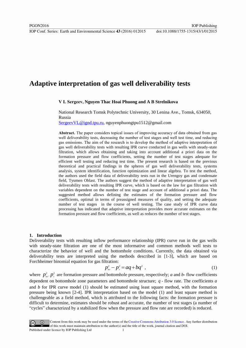
For example, figure 1 shows the initial data for IPR curves for wells 1 and 2, with eight and
seven test stages, respectively.
PGON2016 IOP PublishingIOP Conf. Series: Earth and Environmental Science 43 (2016) 012015 doi:10.1088/1755-1315/43/1/012015
3
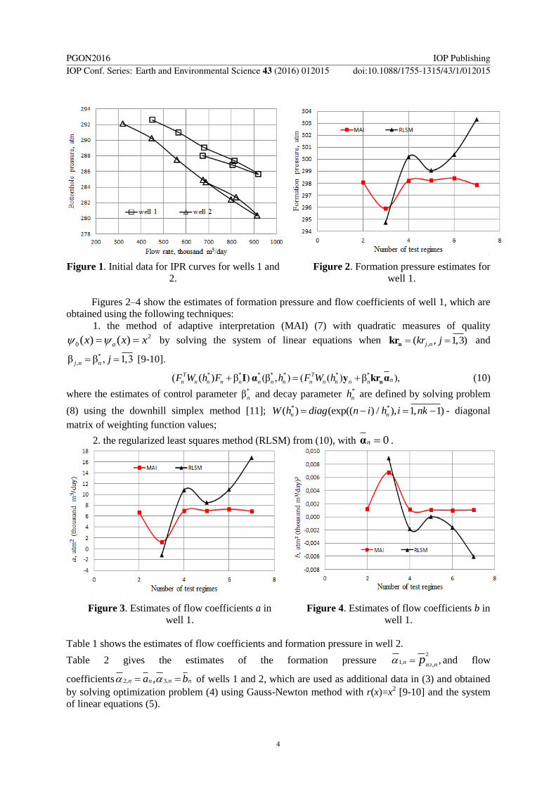
Figure 1. Initial data for IPR curves for wells 1 and
2.
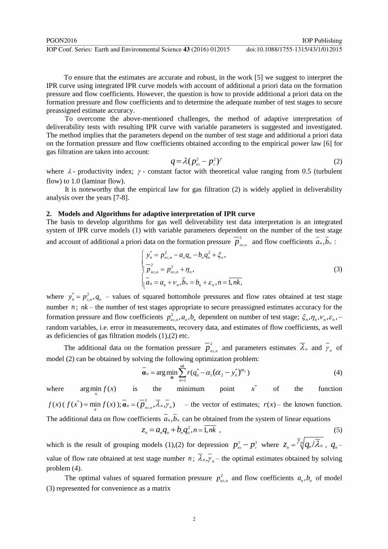
Figure 2. Formation pressure estimates for
well 1.
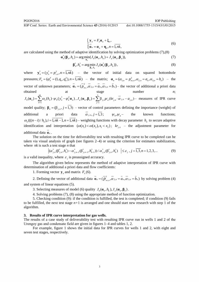
Figures 2–4 show the estimates of formation pressure and flow coefficients of well 1, which are
obtained using the following techniques:
1. the method of adaptive interpretation (MAI) (7) with quadratic measures of quality 2
0( ) ( )ax x x by solving the system of linear equations when ,( , 1,3)j nkr j nkr and
*
,β β , 1,3j n n j [9-10].
* * * * * * *( ( ) β ) (β , ) ( ( ) β ),T Tnn n n n n n n n n n n n nF W h F h F W h nI α y kr α (10)
where the estimates of control parameter *βn and decay parameter *
nh are defined by solving problem
(8) using the downhill simplex method [11]; * *( ) (exp(( ) / ), 1, 1)n nW h diag n i h i nk - diagonal
matrix of weighting function values;
2. the regularized least squares method (RLSM) from (10), with 0n α .
Figure 3. Estimates of flow coefficients a in
well 1.
Figure 4. Estimates of flow coefficients b in
well 1.
Table 1 shows the estimates of flow coefficients and formation pressure in well 2.
Table 2 gives the estimates of the formation pressure 2
1, ,,n пл n
p and flow
coefficients 2, 3,,n n n na b of wells 1 and 2, which are used as additional data in (3) and obtained
by solving optimization problem (4) using Gauss-Newton method with r(x)=x2 [9-10] and the system
of linear equations (5).
PGON2016 IOP PublishingIOP Conf. Series: Earth and Environmental Science 43 (2016) 012015 doi:10.1088/1755-1315/43/1/012015
4
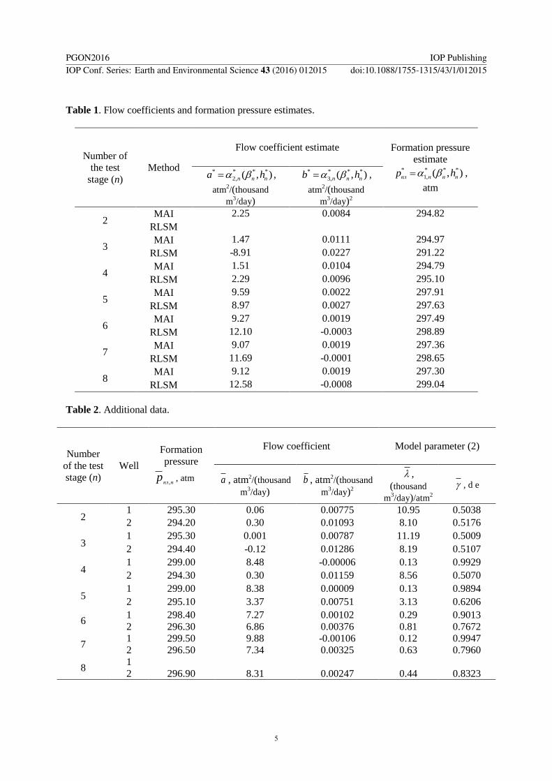
Table 1. Flow coefficients and formation pressure estimates.
Number of
the test
stage (n)
Method
Flow coefficient estimate Formation pressure
estimate * * * *
1, ( , )пл n n np h ,
atm
** * *
2, ( , )n n na h ,
atm2/(thousand
m3/day)
** * *
3, ( , )n n nb h ,
atm2/(thousand
m3/day)2
2 MAI 2.25 0.0084 294.82
RLSM
3 MAI 1.47 0.0111 294.97
RLSM -8.91 0.0227 291.22
4 MAI 1.51 0.0104 294.79
RLSM 2.29 0.0096 295.10
5 MAI 9.59 0.0022 297.91
RLSM 8.97 0.0027 297.63
6 MAI 9.27 0.0019 297.49
RLSM 12.10 -0.0003 298.89
7 MAI 9.07 0.0019 297.36
RLSM 11.69 -0.0001 298.65
8 MAI 9.12 0.0019 297.30
RLSM 12.58 -0.0008 299.04
Table 2. Additional data.
Number
of the test
stage (n)
Well
Formation
pressure
,пл np , atm
Flow coefficient Model parameter (2)
a , atm2/(thousand
m3/day)
b , atm2/(thousand
m3/day)2
,
(thousand
m3/day)/atm
2
, d e
2 1 295.30 0.06 0.00775 10.95 0.5038
2 294.20 0.30 0.01093 8.10 0.5176
3 1 295.30 0.001 0.00787 11.19 0.5009
2 294.40 -0.12 0.01286 8.19 0.5107
4 1 299.00 8.48 -0.00006 0.13 0.9929
2 294.30 0.30 0.01159 8.56 0.5070
5 1 299.00 8.38 0.00009 0.13 0.9894
2 295.10 3.37 0.00751 3.13 0.6206
6 1 298.40 7.27 0.00102 0.29 0.9013
2 296.30 6.86 0.00376 0.81 0.7672
7 1 299.50 9.88 -0.00106 0.12 0.9947
2 296.50 7.34 0.00325 0.63 0.7960
8 1
2 296.90 8.31 0.00247 0.44 0.8323
PGON2016 IOP PublishingIOP Conf. Series: Earth and Environmental Science 43 (2016) 012015 doi:10.1088/1755-1315/43/1/012015
5
It is noteworthy that when the coefficient of model (2) approaches 1, the flow coefficient b
of model (1) approaches 0 (the laminar flow in the well).
As can be seen in figures 2–4 and table 1, the suggested method of adaptive interpretation
with account of additional data allows obtaining more accurate estimates of the formation pressure and
flow coefficients with less amount of field data compared to the method of least squares. For example,
for the adaptive interpretation method three test stages are enough (see figures 2–4 and table 1).
4. Conclusion To overcome the challenges of interpreting deliverability tests with resulting IPR curve of gas wells,
the method of adaptive interpretation with account of additional a priori data has been suggested. This
method allows:
1. Obtaining additional a priori data on the formation pressure and flow coefficients.
2. Defining optimal, in terms of preassigned measures of quality, estimates of the formation
pressure and flow coefficients within the period of test time.
3. Setting the number of test stages adequate for efficient well testing.
The case study of IPR curve interpretation for two wells of the Urengoy gas and condensate
field has indicated that adaptive interpretation provides robust and more accurate estimates of the
formation pressure and flow coefficients, as well as allows reducing the number of test stages.
References
[1] Houpert A 1959 Revue de L’Institut Francais du Petrole. On the flow of gases in porous media.
Vol. 14 (11) pp. 1468-1684. [2] Aliev Z S, Gritsenko A I et al 1995 Moscow Nauka. Guidelines for Well Testing. pp. 523. [3] Aliev Z S and Zotova G A 1980 Moscow Nauka. Gas reservoir and Well Testing: Handbook.
pp. 301. [4] Akhmedov K S, Gasumov R A and Tolpaev V A 2011 Technique of data processing of wells
hydrodynamic studies Petroleum Engineering. Vol. 3 pp. 8–11. [5] Nguyen Th H Ph and Sergeev V L 2015 Bulletin of the Tomsk Polytechnic University:
Georesources Engineering. . Identification of IPR curve for interpreting gas well deliverability
tests. Vol. 326 (12) pp. 54–59. [6] Rawlin E L and Schellhardt M A 1936 United States Bureau of Mines, Monograph 7. Back
pressure data on natural gas wells and their application to production practices. pp. 210. [7] Al-Subaie A A, Al-Anazi B D and Al-Anazi A F 2009 Learning from modified isochronal test
analysis Middle East gas well case study Nafta Scientific Journal 60 pp 405–415 [8] AL-Attar H and Al-Zuhair S 2009 Journal of Petroleum Science and Engineering. A general
approach for deliverability calculations of gas wells. Vol. 67 pp. 97–104. [9] Sergeev V L 2011 TPU Publishing House. Integrated Systems of Identification. pp. 198. [10] Polishchuk V I and Sergeev V L 2015 Journal of Siberian Federal University: Mathematics &
Physics. Adaptive identication method of a signal from stray field magnetic sensor for
turbogenerator diagnostics. Vol. 8 (2) pp. 201–207. [11] Letova T A and Panteleev A V 2002 Moscow: Vysshaya Shkola. Optimization Methods:
Examples and Problems. pp. 544.
PGON2016 IOP PublishingIOP Conf. Series: Earth and Environmental Science 43 (2016) 012015 doi:10.1088/1755-1315/43/1/012015
6