Adaptive Four Legged Locomotion Control Based on Nonlinear ... · Adaptive Four Legged Locomotion...

Preprint May 21, 2006

To appear in Proceedings of The Ninth International Conference on the SIMULATION OF ADAPTIVE BEHAVIOR -- SAB’06

(c) MIT Press

Adaptive Four Legged Locomotion ControlBased on Nonlinear Dynamical Systems

Giorgio Brambilla, Jonas Buchli, Auke Jan Ijspeert

Biologically Inspired Robotic Group (BIRG),Ecole Polytechnique Federale de Lausanne (EPFL),

Station 14, CH-1015 Lausanne, [email protected], {jonas.buchli, auke.ijspeert}@epfl.ch

http://birg.epfl.ch/

Abstract. Dynamical systems have been increasingly studied in the lastdecade for designing locomotion controllers. They offer several advan-tages over previous solutions like synchronization, smooth transitionsunder parameter variation, and robustness. In this paper, we present anadaptive locomotion controller for four-legged robots. The controller iscomposed of a set of coupled nonlinear dynamical systems. Using ourcontroller the robot is capable of adapting its locomotion to the phys-ical properties of the robot, in particular its resonant frequency. Ourapproach aims at developing an on-line learning system that attemptsto minimize the energy necessary for the gait. We have implemented themodel both in a simulated physical environment (Webots) and on a SonyAibo robot. We present a series of experiments which demonstrate howthe controller can tune its frequency to the resonant frequency of therobot, and modify it when the weight of the robot is changed.

1 Introduction

Nonlinear dynamics is ubiquitous in the physical and in the biological world.Nonlinear dynamics theory has provided us with new tools to understand com-plex phenomena that were difficult to explain before. It can be used to modelcompetition in predator-prey systems, emergent behavior in collective systems,growth of biological organisms, the production of rhythmic patterns in the heart[10] and in the spinal cord for locomotion [9, 7], to name a few examples.

In this article, we explore how a nonlinear dynamical system implemented asa system of coupled oscillators can be designed (1) to control walking gaits ofcompliant four-legged robots, and (2) to continuously tune important parameterssuch as the frequency of oscillations to (possibly time-varying) properties of thebody. In particular, we aim at designing adaptive controllers in which the adap-tive process is embedded in the dynamical system (i.e. expressed as differentialequations) rather than in a separate learning or optimization algorithm.

To produce locomotion, a controller must be capable of generating a rhythmicand coordinated behavior. Nonlinear dynamical systems such as systems of cou-pled oscillators present several advantages over alternative approaches (e.g. gait



(c) MIT Press

2 Giorgio Brambilla, Jonas Buchli, Auke Jan Ijspeert

tables or sine-based trajectory generators) to generate gaits for a robot. Theyallow to harmoniously interact with the environment, they can create limit cyclebehavior, they allow smooth modulations of the trajectories, and they make theemergence of new behaviors possible. Moreover, some dynamical systems, likeAdaptive Frequency Oscillators (AFOs) [5, 15] are interesting because of theiradaptive properties.

The controller we propose is suitable for robots with compliant (i.e. elastic)components. It adapts the walking frequency to resonant frequencies of the robotin order to minimize the amount of energy required to move forward. Hopfoscillators and adaptive frequency oscillators are used as building blocks in thecontroller. Adaptation is embedded in the dynamical systems, and no externaloptimization is required. Moreover, adaptation is not a batch process, and thecontroller adapts its parameters online using proprioceptive signals.

The robot locomotion is based on two different kinds of joints: knees - pas-sively controlled by springs, and hips - actively controlled by servos. The robotswings on the knees behaving like an inverted pendulum. A Hopf oscillator [11]controls each hip. Each of these oscillators is coupled to the other hips for inter-limbs gait coordination. Moreover, each hip is coupled in phase to the relativeknee. This movement coordination permits to recycle the potential energy of theknee springs to push the robot forward. Furthermore, an Adaptive FrequencyOscillator (AFO) tunes its frequency to the knee oscillations, and this frequencyis used for the hip oscillators. This controller has two feedback loops: one per-mits phase synchronization to proprioceptor signals and the second frequencyadaptation.

In the rest of the article, we describe our implementation of this system for asimulated and a real Aibo robot (Section 2). Experiments in simulation (Section3) and in the real world (Section 4) demonstrate how the system is capable ofproducing efficient walking gaits that are tuned to the resonant frequency of therobot, and that are continuously adjusted to changing body properties.

2 Adaptive Four Legged Locomotion Model

In this section we describe the main elements of our model. First, we explain whatproperties make a good locomotion controller and our approach to building one.Second, we describe the mechanical specifications the robot shall satisfy. Third,we introduce our CPG (Central Pattern Generator), a central component in ourlocomotion model. Eventually, we elaborate on the adaptive equations, whichevolve the walking frequency parameter depending on the physical properties ofthe robot.

2.1 Mechanical Model

We propose a locomotion controller for four legged robots. Every limb has twojoints: the upper one (hip) and the lower one (knee). Every hip is actively con-trolled and is composed of: a servo (actuator), and an encoder (angle sensor).Every lower joint is passively controlled and is composed of: a spring-damper



(c) MIT Press

Adaptive Four Legged Locomotion Control 3

system (actuator), and an encoder (angle sensor). The controller receives infor-mation from the knee and only controls the hip angle to produce locomotion.The body behaves like an inverted pendulum. Our controller does not explicitelydeal with: inertial forces, moments of inertia, static and dynamic forces, and con-tact ground areas. We will call this mechanical framework ”elastic locomotionframework.” The ideas introduced by Blickhan [2] and by Fukuoka [8] inspiredthis framework.

Our controller reproduces a walking gait. Walking is easy to implement inthis framework, and seems to be the most energy efficient gait compared to trotand gallop [12]. For reasons of stability the terminal limbs are oriented in forwarddirection, as in Figure 1. In fact, if the limbs were turned backwards, the fourlegged robot would tumble and fall during the swing phase. A spring-damperrotational system produces in the knee torques proportional to two components:the angle (γ, i.e. the spring torque) and the the angular velocity (γ, i.e. theviscous damping force): T = kγ − dγ, where k and d are positive spring anddamper coefficients.

2.2 Approach to learning

A good controller to be used in the elastic locomotion framework allows to recyclethe potential energy stored in the knee spring during the step cycle, convertingit into kinetic energy. Our challenge was to build and tune a controller for ageneral four legged robot without specific body information, that satisfies thefollowing properties: (1a) knees and hips should move at the same frequencyand with a constant phase shift; (1b) the four hips move with a fixed phaseshift depending on the gait; and (1c) the knee resonant frequency depends onthe weight of the robot as well as on the constant of the knee spring (k). Theweight can change during the robot life, and the controller should be able toadapt to it. Our approach is based on nonlinear dynamical systems. There aretwo kinds of dynamical systems of interest to us: (2a) Hopf oscillators [11, 16],which are interesting because of their limit cycle behavior with the possibility ofphase synchronization; and (2b) ”Adaptive Frequency Oscillators” (AFOs) [5,15], which are capable of synchronizing their frequency and phase to an externaloscillating signal. In earlier contributions [6] it has been shown that such systemsin a feedback loop with the mechanical system can indeed adapt to the resonantfrequency of the body. Thus, our controller should satisfy constraints (1a), (1b),and (1c) using dynamical system (2a) and (2b) as building blocks.

2.3 CPG with feedback

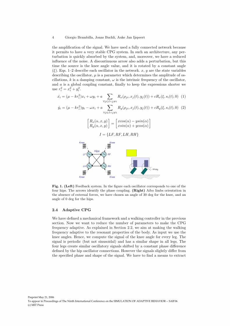
Our controller is composed of a fully connected network of four oscillators in-spired by animal CPGs [4] (see Figure 1). A continuous arrow means that thesignal of the source oscillator at time t is rotated by means of a rotational matrix(R) and summed to the differential equations of the target oscillator. The phaseshifts (ρji) introduced by the rotation matrix are constant and correspond tothe one specified by the walking gait. The coupling values are as in Table 1.Each connection adds a perturbation to the target oscillator that contributes to



(c) MIT Press


the amplification of the signal. We have used a fully connected network becauseit permits to have a very stable CPG system. In such an architecture, any per-turbation is quickly absorbed by the system, and, moreover, we have a reducedinfluence of the noise. A discontinuous arrow also adds a perturbation, but thistime the source is the knee angle value, and it is rotated by a constant angle(ξ). Eqs. 1–2 describe each oscillator in the network. x, y are the state variablesdescribing the oscillator, µ is a parameter which determines the amplitude of os-cillations, k is a damping constant, ω is the intrinsic frequency of the oscillator,and a is a global coupling constant, finally to keep the expressions shorter weuse r2

i = x2i + y2

i .

xi = (µ − kr2i )xi + ωyi + a

∑

∀j∈I∧j 6=i

Rx(ρji, xj(t), yj(t)) + cRx(ξ, si(t), 0) (1)

yi = (µ − kr2i )yi − ωxi + a

∑

∀j∈I∧j 6=i

Ry(ρji, xj(t), yj(t)) + cRy(ξ, si(t), 0) (2)

[

Rx(α, x, y)Ry(α, x, y)

]

=

[

xcos(α) − ysin(α)xsin(α) + ycos(α)

]

I = {LF,RF,LH,RH}

Fig. 1. (Left) Feedback system. In the figure each oscillator corresponds to one of thefour hips. The arrows identify the phase coupling. (Right) Aibo limbs orientation inthe absence of external forces, we have chosen an angle of 30 deg for the knee, and anangle of 0 deg for the hips.

2.4 Adaptive CPG

We have defined a mechanical framework and a walking controller in the previoussection. Now we want to reduce the number of parameters to make the CPGfrequency adaptive. As explained in Section 2.2, we aim at making the walkingfrequency adaptive to the resonant properties of the body. As input we use theknee angles. Hence, we compute the signal of the knee angle for every leg. Thesignal is periodic (but not sinusoidal) and has a similar shape in all legs. Thefour legs create similar oscillatory signals shifted by a constant phase differencedefined by the hip oscillator connections. However the signals slightly differ fromthe specified phase and shape of the signal. We have to find a means to extract



(c) MIT Press


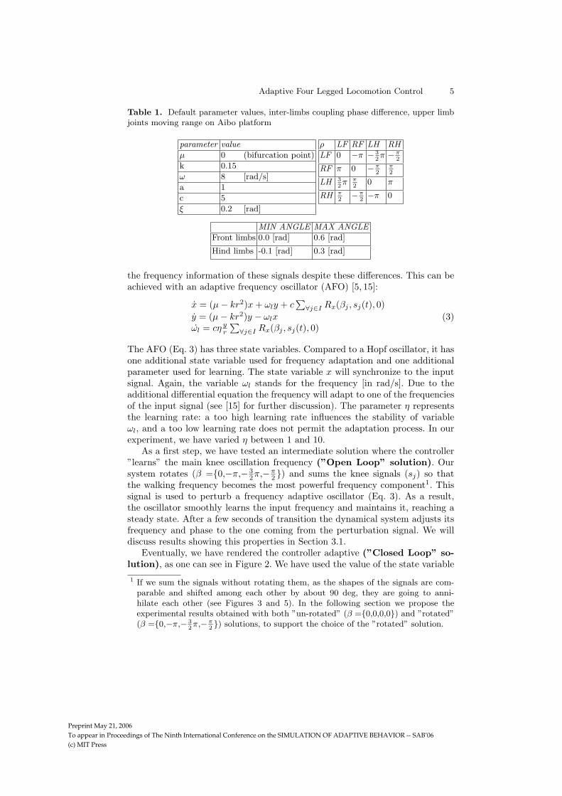
Table 1. Default parameter values, inter-limbs coupling phase difference, upper limbjoints moving range on Aibo platform

parameter value

µ 0 (bifurcation point)

k 0.15

ω 8 [rad/s]

a 1

c 5

ξ 0.2 [rad]

ρ LF RF LH RH

LF 0 −π − 3

2π −π

2

RF π 0 −π

2

π

2

LH 3

2π π

20 π

RH π

2−π

2−π 0

MIN ANGLE MAX ANGLE

Front limbs 0.0 [rad] 0.6 [rad]

Hind limbs -0.1 [rad] 0.3 [rad]

the frequency information of these signals despite these differences. This can beachieved with an adaptive frequency oscillator (AFO) [5, 15]:

x = (µ − kr2)x + ωly + c∑

∀j∈I Rx(βj , sj(t), 0)

y = (µ − kr2)y − ωlx

ωl = cη y

r

∑

∀j∈I Rx(βj , sj(t), 0)(3)

The AFO (Eq. 3) has three state variables. Compared to a Hopf oscillator, it hasone additional state variable used for frequency adaptation and one additionalparameter used for learning. The state variable x will synchronize to the inputsignal. Again, the variable ωl stands for the frequency [in rad/s]. Due to theadditional differential equation the frequency will adapt to one of the frequenciesof the input signal (see [15] for further discussion). The parameter η representsthe learning rate: a too high learning rate influences the stability of variableωl, and a too low learning rate does not permit the adaptation process. In ourexperiment, we have varied η between 1 and 10.

As a first step, we have tested an intermediate solution where the controller”learns” the main knee oscillation frequency (”Open Loop” solution). Oursystem rotates (β ={0,−π,− 3

2π,−π2 }) and sums the knee signals (sj) so that

the walking frequency becomes the most powerful frequency component1. Thissignal is used to perturb a frequency adaptive oscillator (Eq. 3). As a result,the oscillator smoothly learns the input frequency and maintains it, reaching asteady state. After a few seconds of transition the dynamical system adjusts itsfrequency and phase to the one coming from the perturbation signal. We willdiscuss results showing this properties in Section 3.1.

Eventually, we have rendered the controller adaptive (”Closed Loop” so-lution), as one can see in Figure 2. We have used the value of the state variable

1 If we sum the signals without rotating them, as the shapes of the signals are com-parable and shifted among each other by about 90 deg, they are going to anni-hilate each other (see Figures 3 and 5). In the following section we propose theexperimental results obtained with both ”un-rotated” (β ={0,0,0,0}) and ”rotated”(β ={0,−π,− 3

2π,−π

2}) solutions, to support the choice of the ”rotated” solution.



(c) MIT Press


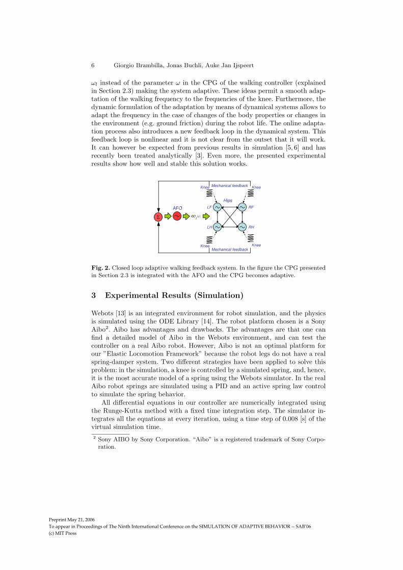
ωl instead of the parameter ω in the CPG of the walking controller (explainedin Section 2.3) making the system adaptive. These ideas permit a smooth adap-tation of the walking frequency to the frequencies of the knee. Furthermore, thedynamic formulation of the adaptation by means of dynamical systems allows toadapt the frequency in the case of changes of the body properties or changes inthe environment (e.g. ground friction) during the robot life. The online adapta-tion process also introduces a new feedback loop in the dynamical system. Thisfeedback loop is nonlinear and it is not clear from the outset that it will work.It can however be expected from previous results in simulation [5, 6] and hasrecently been treated analytically [3]. Even more, the presented experimentalresults show how well and stable this solution works.

Fig. 2. Closed loop adaptive walking feedback system. In the figure the CPG presentedin Section 2.3 is integrated with the AFO and the CPG becomes adaptive.

3 Experimental Results (Simulation)

Webots [13] is an integrated environment for robot simulation, and the physicsis simulated using the ODE Library [14]. The robot platform chosen is a SonyAibo2. Aibo has advantages and drawbacks. The advantages are that one canfind a detailed model of Aibo in the Webots environment, and can test thecontroller on a real Aibo robot. However, Aibo is not an optimal platform forour ”Elastic Locomotion Framework” because the robot legs do not have a realspring-damper system. Two different strategies have been applied to solve thisproblem: in the simulation, a knee is controlled by a simulated spring, and, hence,it is the most accurate model of a spring using the Webots simulator. In the realAibo robot springs are simulated using a PID and an active spring law controlto simulate the spring behavior.

All differential equations in our controller are numerically integrated usingthe Runge-Kutta method with a fixed time integration step. The simulator in-tegrates all the equations at every iteration, using a time step of 0.008 [s] of thevirtual simulation time.

2 Sony AIBO by Sony Corporation. “Aibo” is a registered trademark of Sony Corpo-ration.



(c) MIT Press


3.1 Open Loop Results

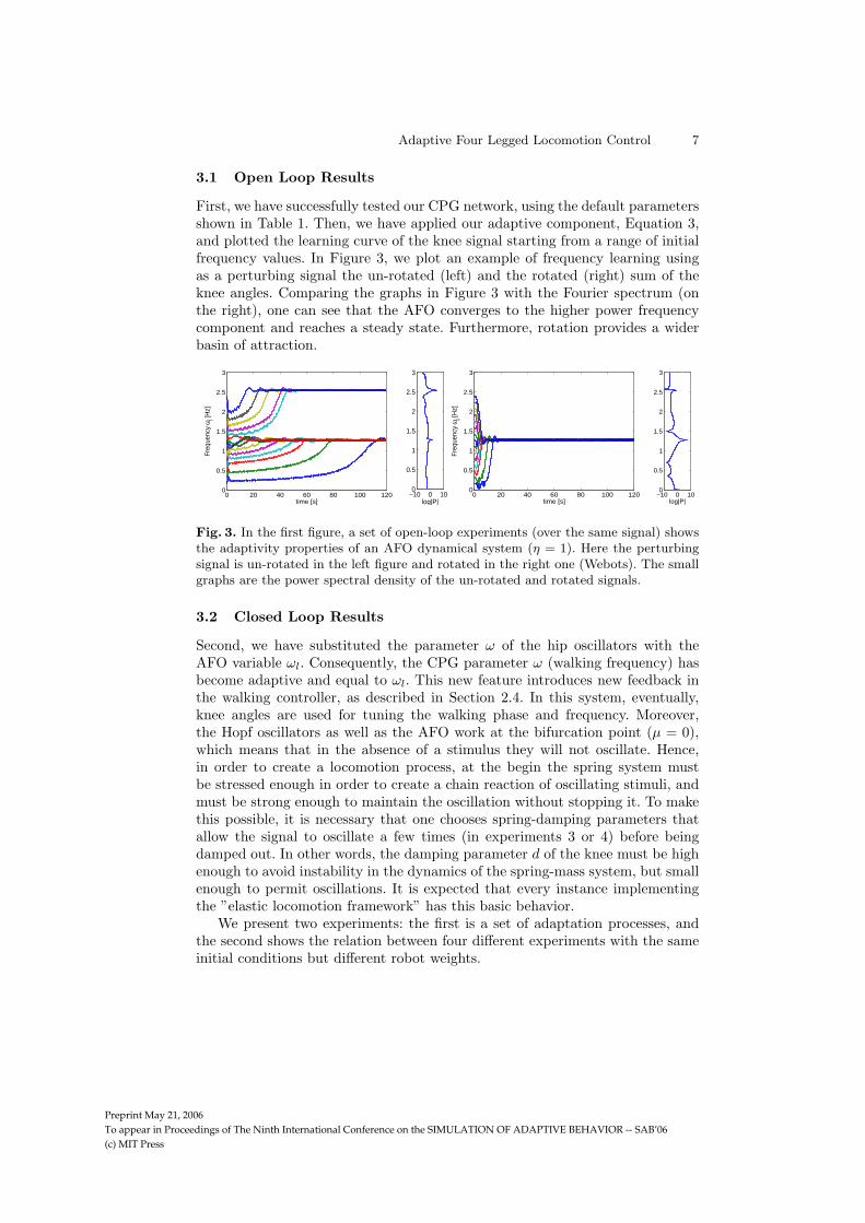
First, we have successfully tested our CPG network, using the default parametersshown in Table 1. Then, we have applied our adaptive component, Equation 3,and plotted the learning curve of the knee signal starting from a range of initialfrequency values. In Figure 3, we plot an example of frequency learning usingas a perturbing signal the un-rotated (left) and the rotated (right) sum of theknee angles. Comparing the graphs in Figure 3 with the Fourier spectrum (onthe right), one can see that the AFO converges to the higher power frequencycomponent and reaches a steady state. Furthermore, rotation provides a widerbasin of attraction.

0 20 40 60 80 100 1200

0.5

1

1.5

2

2.5

3

time [s]

Freq

uenc

y ω l [H

z]

−10 0 100

0.5

1

1.5

2

2.5

3

log|P|0 20 40 60 80 100 120

0

0.5

1

1.5

2

2.5

3

time [s]

Freq

uenc

y ω l [H

z]

−10 0 100

0.5

1

1.5

2

2.5

3

log|P|

Fig. 3. In the first figure, a set of open-loop experiments (over the same signal) showsthe adaptivity properties of an AFO dynamical system (η = 1). Here the perturbingsignal is un-rotated in the left figure and rotated in the right one (Webots). The smallgraphs are the power spectral density of the un-rotated and rotated signals.

3.2 Closed Loop Results

Second, we have substituted the parameter ω of the hip oscillators with theAFO variable ωl. Consequently, the CPG parameter ω (walking frequency) hasbecome adaptive and equal to ωl. This new feature introduces new feedback inthe walking controller, as described in Section 2.4. In this system, eventually,knee angles are used for tuning the walking phase and frequency. Moreover,the Hopf oscillators as well as the AFO work at the bifurcation point (µ = 0),which means that in the absence of a stimulus they will not oscillate. Hence,in order to create a locomotion process, at the begin the spring system mustbe stressed enough in order to create a chain reaction of oscillating stimuli, andmust be strong enough to maintain the oscillation without stopping it. To makethis possible, it is necessary that one chooses spring-damping parameters thatallow the signal to oscillate a few times (in experiments 3 or 4) before beingdamped out. In other words, the damping parameter d of the knee must be highenough to avoid instability in the dynamics of the spring-mass system, but smallenough to permit oscillations. It is expected that every instance implementingthe ”elastic locomotion framework” has this basic behavior.

We present two experiments: the first is a set of adaptation processes, andthe second shows the relation between four different experiments with the sameinitial conditions but different robot weights.



(c) MIT Press


0 20 40 60 80 100 1200

0.5

1

1.5

2

2.5

time [s]

Fre

quen

cy ω

l [Hz]

Initial frequency drops

0 20 40 60 80 1000.8

0.9

1

1.1

1.2

1.3

1.4

1.5

time [s]

Fre

quen

cy ω

l [Hz]

0.6kg

0.9kg

1.2kg

1.5kg

0 20 40 60 80 100 1200

0.050.1

e(t)

time [s]0 20 40 60 80 100

0.02

0.04

0.06

e(t)

time [s]

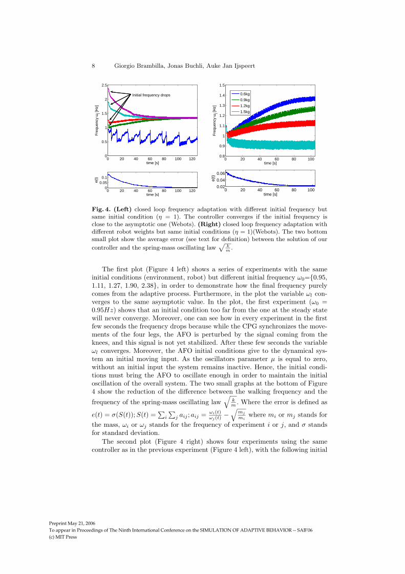
Fig. 4. (Left) closed loop frequency adaptation with different initial frequency butsame initial condition (η = 1). The controller converges if the initial frequency isclose to the asymptotic one (Webots). (Right) closed loop frequency adaptation withdifferent robot weights but same initial conditions (η = 1)(Webots). The two bottomsmall plot show the average error (see text for definition) between the solution of our

controller and the spring-mass oscillating law√

k

m.

The first plot (Figure 4 left) shows a series of experiments with the sameinitial conditions (environment, robot) but different initial frequency ω0={0.95,1.11, 1.27, 1.90, 2.38}, in order to demonstrate how the final frequency purelycomes from the adaptive process. Furthermore, in the plot the variable ωl con-verges to the same asymptotic value. In the plot, the first experiment (ω0 =0.95Hz) shows that an initial condition too far from the one at the steady statewill never converge. Moreover, one can see how in every experiment in the firstfew seconds the frequency drops because while the CPG synchronizes the move-ments of the four legs, the AFO is perturbed by the signal coming from theknees, and this signal is not yet stabilized. After these few seconds the variableωl converges. Moreover, the AFO initial conditions give to the dynamical sys-tem an initial moving input. As the oscillators parameter µ is equal to zero,without an initial input the system remains inactive. Hence, the initial condi-tions must bring the AFO to oscillate enough in order to maintain the initialoscillation of the overall system. The two small graphs at the bottom of Figure4 show the reduction of the difference between the walking frequency and the

frequency of the spring-mass oscillating law√

km

. Where the error is defined as

e(t) = σ(S(t));S(t) =∑

i

∑

j aij ; aij = ωi(t)ωj(t)

−√

mj

miwhere mi or mj stands for

the mass, ωi or ωj stands for the frequency of experiment i or j, and σ standsfor standard deviation.

The second plot (Figure 4 right) shows four experiments using the samecontroller as in the previous experiment (Figure 4 left), with the following initial



(c) MIT Press


conditions: (1) the robot has an initial frequency of 1.1 Hz. (2) In each of the fourexperiments the robot has a different weight (a) 0.6kg, (b) 0.9kg, (c) 1.2kg, (d)1.5kg. The plot shows how a higher weight leads to a lower walking frequency.This behavior respects the spring-mass law where the resonant frequency can

be calculated as√

km

. These results lead to two conclusions: the robot behaves

like a spring-mass system, and it adapts its walking frequency to the resonantfrequency of the knee. This second experiment shows an interesting property ofour system: online adaptation to the physical properties of the robot. In otherwords, the robot is able to adapt its walking following the weight change duringlife (for ex. payload change).

Integrating the torque on the angle of the four hips and summing the fourvalues, we have computed the energy consumed by the robot. Then, to obtain theefficiency, we have divided the energy over the distance covered by the robot. Wehave proved in simulation that this adaptation permits to save energy (in com-parison to non-adaptive CPG) when loading a payload of 0.6 Kg of about 15%(data not shown). Our adaptive system does not maximize the walking speedbut seems to find a more efficient walking frequency. The frequency found seemsto optimize the conversion of the spring potential energy into kinetic energyto propel the robot forward. Our adaptive system can help make the walkinglocomotion more efficient. This is in line with earlier findings in simulations[6].

4 Experimental Results (Real World)

In this section, we show the experimental results on the Aibo robot. As outlinedin Section 3, the Aibo is not the optimal platform to implement the ”elastic lo-comotion framework,” since it has activated knee joints, it does not have passivesprings in the knee joints. In order to simulate the spring law in the knee joints,we have added controllers for the those joints such that the to a large extent theknees behave like a spring, and thus the robot corresponds to the requirementsas stated in the ”elastic locomotion framework”. As in the case of the simulation,the equations are numerically integrated with a Runge-Kutta algorithm with afixed time step of 0.008 [s]. The design of Aibo controller also takes care of fur-ther implementation problems occurring when simulating a spring law such asencoder resolution and accuracy, mechanical gear backlash, digital system delay,system identification and other problems (cf. [1] for more details). In the follow-ing two sections we have repeated the two simulation experiments on real worldAibo.

4.1 Open Loop Results

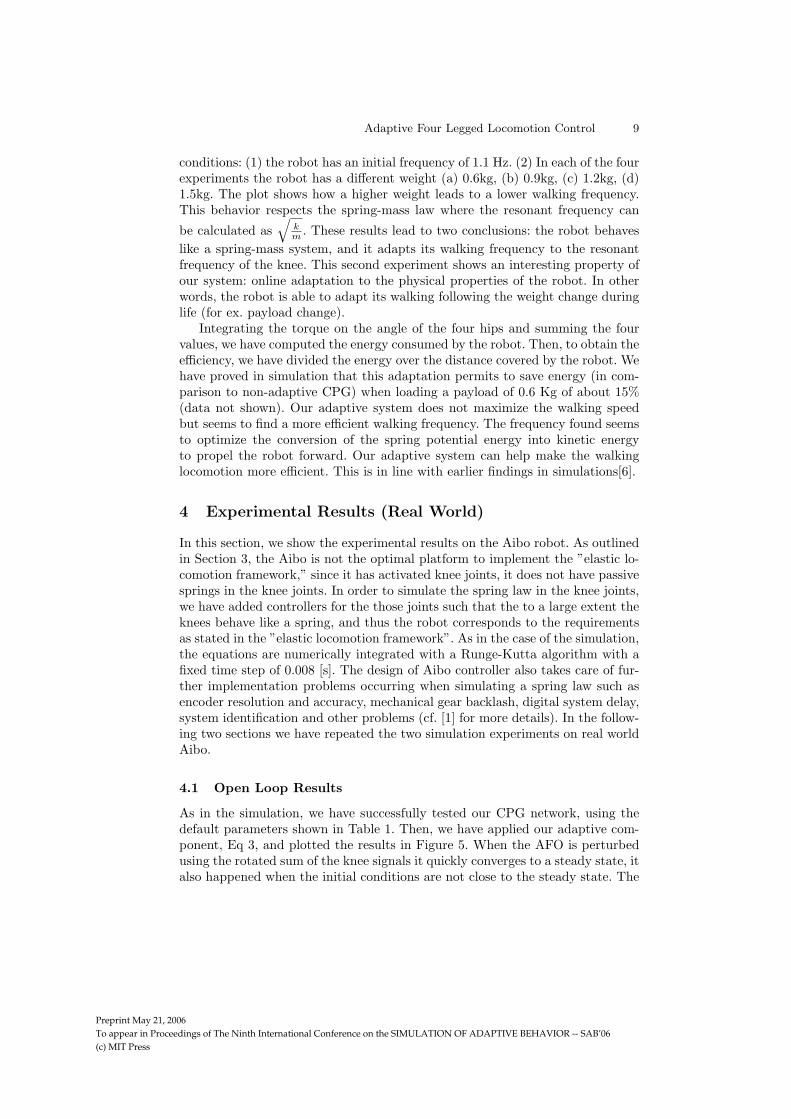
As in the simulation, we have successfully tested our CPG network, using thedefault parameters shown in Table 1. Then, we have applied our adaptive com-ponent, Eq 3, and plotted the results in Figure 5. When the AFO is perturbedusing the rotated sum of the knee signals it quickly converges to a steady state, italso happened when the initial conditions are not close to the steady state. The



(c) MIT Press


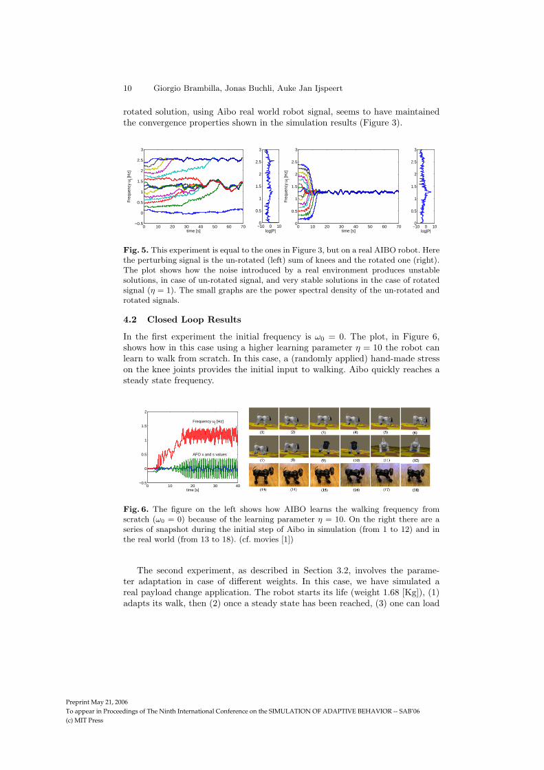
rotated solution, using Aibo real world robot signal, seems to have maintainedthe convergence properties shown in the simulation results (Figure 3).

0 10 20 30 40 50 60 70−0.5

0

0.5

1

1.5

2

2.5

3

time [s]

Freq

uenc

y ω l [H

z]

−10 0 100

0.5

1

1.5

2

2.5

3

log|P|0 10 20 30 40 50 60 70

0

0.5

1

1.5

2

2.5

3

time [s]

Freq

uenc

y ω l [H

z]

−10 0 100

0.5

1

1.5

2

2.5

3

log|P|

Fig. 5. This experiment is equal to the ones in Figure 3, but on a real AIBO robot. Herethe perturbing signal is the un-rotated (left) sum of knees and the rotated one (right).The plot shows how the noise introduced by a real environment produces unstablesolutions, in case of un-rotated signal, and very stable solutions in the case of rotatedsignal (η = 1). The small graphs are the power spectral density of the un-rotated androtated signals.

4.2 Closed Loop Results

In the first experiment the initial frequency is ω0 = 0. The plot, in Figure 6,shows how in this case using a higher learning parameter η = 10 the robot canlearn to walk from scratch. In this case, a (randomly applied) hand-made stresson the knee joints provides the initial input to walking. Aibo quickly reaches asteady state frequency.

0 10 20 30 40−0.5

0

0.5

1

1.5

2

time [s]

AFO x and s values

Frequency ωl [Hz]

Fig. 6. The figure on the left shows how AIBO learns the walking frequency fromscratch (ω0 = 0) because of the learning parameter η = 10. On the right there are aseries of snapshot during the initial step of Aibo in simulation (from 1 to 12) and inthe real world (from 13 to 18). (cf. movies [1])

The second experiment, as described in Section 3.2, involves the parame-ter adaptation in case of different weights. In this case, we have simulated areal payload change application. The robot starts its life (weight 1.68 [Kg]), (1)adapts its walk, then (2) once a steady state has been reached, (3) one can load



(c) MIT Press


0 10 20 30 40 50 60 70−0.5

0

0.5

1

1.5

2

2.5

time [s]

Freq

uenc

y ω l [H

z]

0 50 100 150 200

1

1.1

1.2

1.3

time [s]

Freq

uenc

y ω l [H

z]

↓ (1) Start Adaptation↓ (2) Unload Steady State

↑ (3) Loading 0.4 [Kg]

↑ (4) Load Steady State

↑ (5) Unload

↓ (6) Unload Steady State

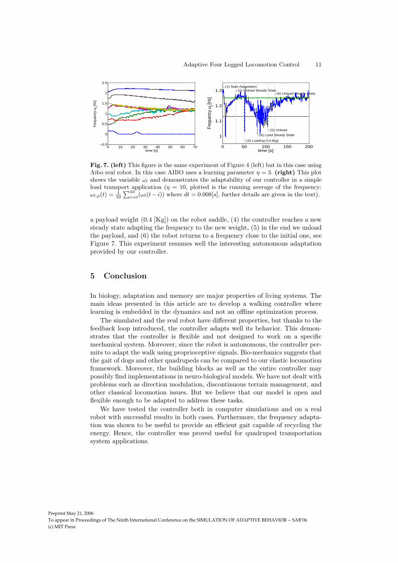
Fig. 7. (left) This figure is the same experiment of Figure 4 (left) but in this case usingAibo real robot. In this case AIBO uses a learning parameter η = 3. (right) This plotshows the variable ωl and demonstrates the adaptability of our controller in a simpleload transport application (η = 10, plotted is the running average of the frequency:ωl,p(t) = 1

50

∑

50

i=0(ωl(t− i)) where dt = 0.008[s], further details are given in the text).

a payload weight (0.4 [Kg]) on the robot saddle, (4) the controller reaches a newsteady state adapting the frequency to the new weight, (5) in the end we unloadthe payload, and (6) the robot returns to a frequency close to the initial one, seeFigure 7. This experiment resumes well the interesting autonomous adaptationprovided by our controller.

5 Conclusion

In biology, adaptation and memory are major properties of living systems. Themain ideas presented in this article are to develop a walking controller wherelearning is embedded in the dynamics and not an offline optimization process.

The simulated and the real robot have different properties, but thanks to thefeedback loop introduced, the controller adapts well its behavior. This demon-strates that the controller is flexible and not designed to work on a specificmechanical system. Moreover, since the robot is autonomous, the controller per-mits to adapt the walk using proprioceptive signals. Bio-mechanics suggests thatthe gait of dogs and other quadrupeds can be compared to our elastic locomotionframework. Moreover, the building blocks as well as the entire controller maypossibly find implementations in neuro-biological models. We have not dealt withproblems such as direction modulation, discontinuous terrain management, andother classical locomotion issues. But we believe that our model is open andflexible enough to be adapted to address these tasks.

We have tested the controller both in computer simulations and on a realrobot with successful results in both cases. Furthermore, the frequency adapta-tion was shown to be useful to provide an efficient gait capable of recycling theenergy. Hence, the controller was proved useful for quadruped transportationsystem applications.



(c) MIT Press


Acknowledgments

G.B. wishes to especially thank his friend, Fabrizio Patuzzo, for his encourage-ment, support, and review during the entire work. This work was made possiblethanks to a Young Professorship Award to Auke Ijspeert from the Swiss NationalScience Foundation.

References

1. Movies and more technical details of the implementation are available online athttp://birg.epfl.ch/page57636.html.

2. R. Blickhan. The spring-mass model for running and hopping. J. Biomechanics,22(11–12):1217–1227, 1989.

3. J. Buchli, F. Iida, and A.J. Ijspeert. Finding resonance: Adaptive frequency oscil-lators for dynamic legged locomotion. Submitted.

4. J. Buchli and A.J. Ijspeert. Distributed central pattern generator model forrobotics application based on phase sensitivity analysis. In Proceedings BioADIT2004, volume 3141 of Lecture Notes in Computer Science, pages 333–349. SpringerVerlag Berlin Heidelberg, 2004.

5. J. Buchli and A.J. Ijspeert. A simple, adaptive locomotion toy-system. In S. Schaal,A.J. Ijspeert, A. Billard, S. Vijayakumar, J. Hallam, and J.A. Meyer, editors, FromAnimals to Animats 8. Proceedings of the Eighth International Conference on theSimulation of Adaptive Behavior (SAB’04), pages 153–162. MIT Press, 2004.

6. J. Buchli, L. Righetti, and A.J. Ijspeert. A dynamical systems approach to learning:a frequency-adaptive hopper robot. In Proceedings ECAL 2005, Lecture Notes inArtificial Intelligence, pages 210–220. Springer Verlag, 2005.

7. A.H. Cohen and D.L. Boothe. Sensorimotor interactions during locomotion: prin-ciples derived from biological systems. Autonomous Robots, 7(3):239–245, 1999.

8. Y. Fukuoka, H. Kimura, and A.H. Cohen. Adaptive dynamic walking of aquadruped robot on irregular terrain based on biological concepts. The Inter-national Journal of Robotics Research, 3–4:187–202, 2003.

9. S. Grillner. Control of locomotion in bipeds, tetrapods and fish. In V.B. Brooks,editor, Handbook of Physiology, The Nervous System, 2, Motor Control, pages1179–1236. American Physiology Society, Bethesda, 1981.

10. J. Honerkamp. The heart as a system of coupled nonlinear oscillators. J MathBiol, 18(1):69–88, 1983.

11. E. Hopf. Abzweigung einer periodischen Losung von einer stationaren Losung einesDifferentialsystems. Ber. Math.-Phys., Sachs. Akad. d. Wissenschaften, Leipzig,pages 1–22, 1942.

12. T. McGeer. Passive dynamic walking. International Journal of Robotics Research,9:62–82, 1990.

13. O. Michel. Webots: Professional mobile robot simulation. International Journalof Advanced Robotic Systems, 1(1):39–42, 2004.

14. Russell Smith & others. Open Dynamics Engine. Available online athttp://ode.org.

15. L. Righetti, J. Buchli, and A.J. Ijspeert. Dynamic hebbian learning in adaptivefrequency oscillators. Physica D, 216(2):269–281, 2006.

16. S. Strogatz. Nonlinear Dynamics and Chaos. With applications to Physics, Biology,Chemistry, and Engineering. Addison Wesley Publishing Company, 1994.

Adaptive Four Legged Locomotion Control Based on Nonlinear ... · Adaptive Four Legged Locomotion...

Documents

Transcript of Adaptive Four Legged Locomotion Control Based on Nonlinear ... · Adaptive Four Legged Locomotion...