LEARNING ABOUT CONTROL OF LEGGED LOCOMOTION USING A

HEXAPOD ROBOT WITH COMPLIANT PNEUMATIC ACTUATORS

by

GABRIEL MARTIN NELSON

Submitted in partial fulfillment of the requirements

For the degree of Doctor of Philosophy

Thesis Advisor: Dr. Roger D. Quinn

Department of Mechanical and Aerospace Engineering

CASE WESTERN RESERVE UNIVERSITY

May, 2002

Copyright 2002 by Gabriel Martin Nelson All rights reserved

CASE WESTERN RESERVE UNIVERSITY

SCHOOL OF GRADUATE STUDIES

We hereby approve the dissertation of

GABRIEL MARTIN NELSON

candidate for the Doctor of Philosophy degree *.

Committee Chair: ________________________________________________ Dr. Roger D. Quinn Dissertation Advisor Professor, Department of Mechanical and Aerospace Engineering

Committee: _____________________________________________________ Dr. Joseph M. Mansour Professor, Department of Mechanical and Aerospace Engineering

Committee: _____________________________________________________ Dr. Stephen M. Phillips Professor, Department of Electrical Engineering and Computer Science

Committee: _____________________________________________________ Dr. Roy E. Ritzmann Professor, Department of Biology

May, 2002

*We also certify that written approval has been obtained for any proprietary material contained therein.

Waiver of Reproduction Rights

To Stephanie

Do you see a man wise in his own eyes? There is more hope for a fool than for him.

Proverbs 26:12

For the LORD gives wisdom, and from His mouth come

knowledge and understanding. Proverbs 2:6

vi

Table of Contents

Table of Contents.................................................................................................................. vi List of Tables .......................................................................................................................viii List of Figures ....................................................................................................................... ix Acknowledgements............................................................................................................. xvi Abstract ...............................................................................................................................xviii

1 Introduction .........................................................................................................................1 1.1 Robot 3............................................................................................................2 1.2 Thesis Outline.................................................................................................5 Works Cited .............................................................................................................7

2 Review ...................................................................................................................................8

Works Cited ...........................................................................................................18 3 Posture Control ............................................................................................................... 22

3.1 Single Leg Mechanics..................................................................................25 3.2 Somatosensory Feedback of Body Position ...............................................27 3.3 Multi-leg Mechanics ....................................................................................28 3.4 Solving the Force Distribution Problem .....................................................29 3.5 Results...........................................................................................................34 3.6 Conclusions ..................................................................................................37 Works Cited ...........................................................................................................39

4 Posture Control Implementation Issues ....................................................................... 41

4.1 Original Hardware Setup .............................................................................41 4.2 Open-loop force control...............................................................................43 4.3 Conclusion ....................................................................................................47 Works Cited ...........................................................................................................47

5 Inverse kinematics............................................................................................................ 49

5.1 General Notation ..........................................................................................49 5.2 Redundant limb kinematics .........................................................................50 5.3 A Practical Goal: Maximize Leg Mobility .................................................52 5.4 A Simple Redundant Manipulator ..............................................................53 5.5 Ways of finding equilibrium solutions for both the SRM and Robot 3....63 5.6 A Biological Perspective: Animal-Like Movements.................................73 5.7 Neural-Network Implementation ................................................................75 5.8 Results and Conclusions..............................................................................77 Works Cited ...........................................................................................................82

6 Local Control Implementation Details ......................................................................... 86

6.1 Improvements in the Robot 3 control system.............................................86

vii

6.2 Pulse actuation implementation issues .......................................................96 Works Cited .........................................................................................................110

7 Conclusions and Future Work ..................................................................................... 113

7.1 Future Work................................................................................................114 7.1.1 Open-loop control issues ....................................................................114 7.1.2 What about those strain gages? ..........................................................115 7.1.3 Lead compensation..............................................................................116 7.1.4 Positive load feedback ........................................................................121 7.1.5 Revalving the robot.............................................................................124

7.2 Conclusions ................................................................................................124 7.3 Some lessons learned from Robot 3..........................................................128

7.3.1 Carefully consider using pneumatic pulse actuation.........................128 7.3.2 Carefully consider which sensors to use............................................129 7.3.3 Simulate ...............................................................................................129 7.3.4 Strive for modularity and ruggedness................................................130 7.3.5 Successful gait coordination is not the same as successful walking130 7.3.6 Developing the basic control system takes time ...............................131 7.3.7 Acoustic aesthetics matter ..................................................................132

Works Cited .........................................................................................................132 Appendix............................................................................................................................. 133 Bibliography....................................................................................................................... 134

viii

List of Tables

Table 1: Basic legged robot classifications. ..........................................................................8

Table 2: Types of biomimetic articulated limb legged robots............................................11

ix

List of Figures

Figure 1: Robot 3. Robot 3 is a 17-to-1 robot-to-cockroach scale model of Blaberus discoidalis (shown at right). It is approximately 30 inches long and weighs about 30 pounds. It has 24 joints, each independently actuated with one or more double acting pneumatic cylinders. Single-turn potentiometers and half-bridge strain gage load cells provide joint angle sensing and three-axis load sensing at each foot, respectively. .................3

Figure 2: Strain gages on a Robot 3 leg. Three pairs of strain gages measure bending at three different points on the robot leg. The In-Plane-Femur (IPF) gages at the proximal end of the femur, and the In-Plane-Tibia (IPT) gages at the proximal end of the tibia, measure bending about axes perpendicular to the plane formed by the femur and tibia. The Out-of-Plane-Tibia (OPT) gages measure bending at the proximal end of the tibia about an axis lying in the plane formed by the femur and tibia. .........................................................................................................................5

Figure 3: Whegs. A reduced-actuation hexapod vehicle built at the CWRU BioRobotics Lab. A single motor drives six “whegs” – or wheel-legs – which are phased in a nominal tripod gait. A torsional compliance in the drive shaft at each wheg allows for phasing variations such as those needed for climbing obstacles. Whegs moves at about three body-lengths per second (60 in/s), and can climb barriers greater than its body height............................................................................................................10

Figure 4: Protobot is an 18 DOF pneumatically actuated hexapod robot modeled after Periplaneta americana. ...............................................................................13

Figure 5: RHex is a typical example of a Type 3 robot. Each leg is a single compliant spoke, driven, at the hip, by a motor under PD control. The spoke swings in a full circle parallel to the sagittal plane of the robot. RHex is a simple and reliable hexapod robot with good rough terrain capabilities.............................................................................................................16

Figure 6: Single leg mechanics notation. The body reference frame consists of the x1 ≡ rostral or direction of travel, y1 ≡ lateral or left, z1 ≡ vertical. Each body (1 through 4) contains its own body-fixed reference frame. The vector definitions (Li and Wi) are given in the text.....................................25

Figure 7: Single virtual leg model of robot mechanics. Provided with desired virtual forces acting on the body, the posture controller predicts the position of a center of pressure (COP) where a virtual leg would, at that instant, produce those virtual forces. The scheme is repeated for the x-z plane. The virtual leg would also have a foot (not shown) that would produce a desired virtual Mz. ...............................................................................32

x

Figure 8: Disturbance rejection while standing via posture control. While standing, the robot was shoved repeatedly. Each arrow indicates a disturbance. The robot swayed and returned to a nominal standing position. “y pos” indicates the y, or lateral, position (see Figure 6) of the body. “y cop” is the y location of the COP. The COP moved to counteract the disturbances. The COP was slightly negative because the robot perceived a small roll error (lean to left). Stiction in the cylinders caused the initial and final body positions to be slightly different. ................................................................................................................35

Figure 9: Vertical load transfer to move COP. Corresponding to Figure 8, this figure shows how vertical load responsibility was transferred to the left side legs as the COP moves to counteract the disturbances. “left/right n” is the ipsilateral sum of nl values....................................................................35

Figure 10: Robot 3 lifts a 30 pound payload. The payload, which is equivalent to its own weight, is suspended below the robot with cables. The robot is able to perform “push-ups” while doing this. .....................................................36

Figure 11: The overall original posture control system. Computer #2 (PC#2), which was slaved to computer #1 (PC#1), performed PWM on the 48 valves at a frequency of 50 Hz according to commanded duty cycles from PC#1. PC#1, directly reading sensory information from the physical robot, performed posture control calculations and output commanded duty cycles to PC#2.........................................................................41

Figure 12: Original Robot 3 posture control basic electronics. PC#1 was a 133MHz Pentium desktop running the posture controller in DOS. The controller dispatched (unbuffered) commanded duty cycles to PC#2, a 127MHz AMD desktop, via 115200 bps serial communication. PC#1 also read 24 potentiometer signals from an ISA A/D (12 bit) card (original gage signals, which were not used, were one per leg and meant for binary contact sensing only). PC#2, running in DOS, polled a timer card to perform 50 Hz PWM with about a 1% resolution. A digital I/O card drove 48 opto-isolators, which in turn drove the valves of the robot. ...........................................................................................................42

Figure 13: Original duty cycle to force output relationship at 50 Hz PWM. Various cylinder sizes were tested for their steady-state force output as a function of duty cycle at 50 Hz PWM. The curves were then normalized by the theoretical maximum force for that cylinder size, and a sigmoidal curve was fit to the data (Eq. (20)). The inverse of this relationship was used for open-loop force control..............................................44

Figure 14: An extremely simple redundant manipulator (SRM). Joint-space DOF are θ1 and θ2 while there is a single task-space DOF, xd. θ1 is measured from the horizontal and θ2 is relative to link 1 (positive rotations are

xi

CCW according to a right-hand rule, making θ2 negative above). Link lengths are l1 and l2. Linear torsional springs (with constants k1 and k2) acting in joint-space (equilibrium positions 1θ and 2θ not indicated) are resisted by an end effector force, F, in task-space. The relative motion of the block, at the end of link 2, in the slot is frictionless. ............................................................................................................54

Figure 15: Solution manifolds to the forward kinematics of the SRM with l1 = l2 = 1. The xd = 2 manifold (which is just a point) is located at {θ1, θ2} = {0, 0}. The xd = -2 (also just a point) is located at {π, 0}. The remaining manifolds are evenly spaced in task-space at 0.2 intervals between –2 ≤ xd ≤ 2, such that traversing a straight line from {0, 0} to {π, 0}, we cross the following manifolds: xd = 1.8, 1.6, … 0, … -1.6, -1.8. The entire pattern is repeated at 2π intervals in each direction (making the point {-π, 0} also a xd = -2 manifold).............................................57

Figure 16: Loci of all possible solutions to Eq. (33) for the SRM with k1 = k2 = 1,

1θ = π/2, 2θ = -π/2. The reachable joint-space has been limited to 0 < θ1 < π and –π < θ2 < 0 in order to exclude any structural singularities. The two loci have been distinguished as “primary” and “secondary”. The arrow indicates the approximate location on the secondary locus where the augmented Jacobian (see text) becomes singular. Refer to Figure 15 for the xd manifold values. ..................................................................61

Figure 17: Comparison of three inverse kinematic solution methods applied to the SRM. All parameters are set as discussed in Figure 16, Cj is the identity matrix, and the starting position is the unloaded equilibrium position. The goal is to move the end effector from the unloaded equilibrium position (xd = 1) to xd = -1. The quasi-static method is based on a straightforward scheme which simulates the motion of the manipulator quasi-statically with joint-space springs and dampers while an applied force at the end effector drives the system to desired task-space positions. The Seraji method is based on an online redundant manipulator control scheme that controls end effector motion in task-space as well as one or more user-defined “self-motion” task functions. The minimum joint-space velocity method is the standard Moore-Penrose pseudoinverse of the Jacobian with a constant weight matrix. Exact methods are not shown, since they lie directly along the primary locus.......................................................................................................................65

Figure 18: Block diagram of Seraji redundant manipulator control. An augmented task-space vector, Y, consisting of end effector position as well as (N-M) task functions, is fed back for PD control to produce a corrective augmented wrench vector, FA. Augmented Jacobians transform FA into joint torques, τ, and joint positions and velocities into

xii

augmented task-space velocity. KP and KD are NxN matrices of proportional and derivative gains respectively. ..................................................68

Figure 19: Partial overhead view of Robot 3 showing left front leg x-y coordinate system used for inverse kinematics studies. The origin is the body-coxa joint, which is where the leg attaches to the body. This view looks in the –z direction. ......................................................................................77

Figure 20: Desired circular foot path vs. neural-network output. The trained neural-network outputs joint angles for desired foot positions along a 5 inch radius circular path in the x-y plane, with pfoot/d,z = -6 inches below the body-coxa joint. These joint angles result in a slightly distorted actual foot position path. ......................................................................................80

Figure 21: Desired square foot path vs. neural-network output. The trained neural-network outputs joint angles for desired foot positions along a 7x7 inch square path in the x-y plane, with pfoot/d,z = -6 inches below the body-coxa joint. These joint angles result in a slightly distorted actual foot position path. .................................................................................................80

Figure 22: Neural-network to cockroach comparison. Forceps were used to move the tibia-tarsis joint of a deinnervated left front cockroach leg through a walking cycle motion. The motion was filmed and digitized to produce joint angle trajectories (dark lines) and scaled foot motion. This foot motion was then used as input to the neural-network to produce optimal joint angle trajectories for comparison (light lines). The poorer fit of the FT trace may have two possible sources: the joint compliance functions were too simple, or the forceps applied an unknown environmental moment to the tibia. .....................................................................84

Figure 23: Snapshots of Robot 3 air-walking in a tripod gait. The sequence of snapshots, cropped from digital video of the robot, goes from left to right, top to bottom. In the first snapshot, the near-side middle leg is in stance while the front and rear legs transition to swing. In the second snapshot, the front and rear legs are in full swing. In the third snapshot, they transition into stance, while in the fourth snapshot, the middle leg transitions to swing. ..............................................................................................85

Figure 24: Improved basic control system setup. PC#1 (500MHz Pentium), which runs the high level controller (HLC), performs longer latency, higher complexity calculations (such as posture control) and issues any of a variety of commands or guidelines to PC#2 (127MHz AMD) which is running the low level controller (LLC). The HLC is also responsible for setting LLC parameters such as control loop gains and set-points. The LLC performs all data acquisition of sensor feedback and commands the valves of the robot. It also directly copies sensor data to the HLC.....................................................................................................87

xiii

Figure 25: Control system communications structure. The HLC consists of two processes: a lower priority background process running the actual HLC code and a higher priority communications ISR (Com ISR). The LLC consists of three processes: a lower priority background process that performs certain non-time-critical calculations as well as moving data to and from the Com ISR buffers and memory, a middle priority process (the Com ISR), and a high level PWM ISR which does elementary control calculations, A/D conversions and valve commanding. One problem with this setup is that the flow of data to and from the PWM ISR to the HLC is handled by the low priority background process. .............................................................................................88

Figure 26: Improved control system communications structure. This is an improvement on the structure in Figure 25. Now the LLC PWM ISR not only stores sensor data in memory but it also directly copies this same data to the serial communications transmit (Tx) FIFO buffer for immediate dispatch to the HLC. Also, both the HLC and LLC Com ISRs directly access memory through structured buffers. As a result, the LLC background process is no longer involved in data flow. Flow control is implemented from the HLC to the LLC so that the HLC can dump arbitrarily large chunks of data into the Com ISR transmit buffer..........89

Figure 27: Time division multiplexing as applied to Robot 3. At 80 Hz PWM, there are 80 PWM periods in one second. Each PWM period is divided into 125 µs intervals by 100 PWM interrupts, which occur at 8 kHz. The PWM ISR alternates between different tasks on each interrupt. When all the sensors needed for calculating the control law for a group of valves are read (i.e. the duty cycles for the valves that run a joint), the PWM period for those valves begins. There is a one PWM interrupt delay from the beginning (end) of the PWM period and the ON(OFF) valve commands. This is because the valve commands are issued at the beginning of that PWM interrupt in order that the interval timing of the duty cycle be precise. When the PWM period completes, the entire process is repeated................................................................................91

Figure 28: Low level controller details corresponding to Figure 25. See text for details.....................................................................................................................93

Figure 29: Low level controller details corresponding to Figure 26. See text for details.....................................................................................................................95

Figure 30: Relationship between commanded and actual duty cycles due to valve delay properties. The valves are Matrix 750 series (8 channel) three-way solenoid valves. When pressurized to 100 psig, the open delay is approximately 4 ms, while the close delay is slightly under 1 ms.....................97

xiv

Figure 31: The effects of valve delays on actual open and close times at 80 Hz PWM. The bold horizontal lines represent when the valve is energized, while the bold sloped lines represent when the valve is deenergized. The respective light lines represent when the valve opens or closes. Given a commanded duty cycle, the valve takes 32% (4ms) of the PWM period to open from a cold start, and 8% (1ms) to close after being deenergized. For commanded duty cycles above 92%, this close delay advances the open time substantially.........................................................99

Figure 32: Warping valve command times to normalize actual valve open time. By sliding normalized time for commanded duty cycles above 92%, it is possible to cause the valve to open at the same time each PWM period...................................................................................................................100

Figure 33: Valve pretensioning timing curves for 80 Hz predicted PWM. The “New PWM period” is now bounded by when the valve actually opens, not the valve commands. The once-per-PWM-period control loop update is now performed when the valve opens. If the control law calls for duty cycles below the valve open delay (32% at 80 Hz PWM), the valve is deenergized immediately and the active force output of the actuator is negligible...........................................................................................101

Figure 34: Four different pulse actuation schemes. These results are examples taken from the simulation depicted in Figure 35. The input signal is a 15 Hz sinusoid that was chosen to exaggerate the differences between the different schemes. Also, a 50 Hz PWM counter signal (saw-tooth) is shown with the input signal for reference. ....................................................103

Figure 35: Pulse actuation behavior simulation. The “simple PWM” box performs simple PWM (see text) based on a commanded duty cycle (“CDC”) and a PWM frequency (“PWM freq”), outputting a commanded pulse train (“CPT”). The CPT is fed into an “Electromechanical Valve Model” which outputs an actual pulse train (“APT”) which is the actual valve open/close state signal...............................104

Figure 36: Electromechanical valve model. This is the inner workings of the valve model from Figure 35. Based on the value of CPT, the “Charge” or “Discharge” dynamics operate after exchanging their state value at the time of CPT switching. The output of the model is the actual pulse train (“APT”) which is the valve open/close state signal. This model approximates the high duty cycle behavior depicted in Figure 31. .................105

Figure 37: Simulation used to compare the open-loop frequency response of different pulse actuation schemes. Two simplified antagonistic air cylinder models move a lightly damped mass. The cylinders are inflated/exhausted by an electromechanical valve model that is driven with different pulse actuation schemes..............................................................108

xv

Figure 38: Greatly simplified air cylinder model. The inflate dynamics (50/(s+50)) are slightly faster than the exhaust dynamics (30/(s+30)). The output is treated as a gage pressure between 0 and 100 psig....................109

Figure 39: Frequency response performance comparison of pulse actuation schemes using simulation from Figure 37. The magnitude responses are normalized across all schemes using valve curves. Thus better performance is defined as less phase lag (phase closer to zero). In the simulation, the commanded frequency input to PFM was clipped at 100 Hz for the 10 ms pulse scheme, and 200 Hz for the 5 ms pulse scheme.........112

Figure 40: Conceptual system describing ways to improve the performance of Robot 3’s actuators. The inset depicts a mass acted on by an external force and a pneumatic actuator. The actuator consists of passive damping, and an active response that describes how quickly force, due to air pressure, changes inside the actuator. A tendon, with imbedded load sensor, attaches the actuator to the mass. Lead compensation of the position control signal could allow for higher stiffnesses and better disturbance rejection. Positive load feedback can provide rapid load compensation by augmenting both the actuator’s passive damping and the control system’s active stiffness. .................................................................117

Figure 41: Effect of lead compensation on the root locus for the system depicted in Figure 40 with Gf = 0. The goal of the compensation is to allow for a higher position control gain or stiffness (‘K’) by moving the root locus away from the right-half plane. The hatched region represents the desired closed-loop response. The compensated system can achieve a much higher stiffness while maintaining a desirable response of damping ratio, ζ = 0.5. Lead compensation basically approximates derivative control. ...............................................................................................119

Figure 42: The response of the lead compensator ((1/35 s + 1)/(1/85 s + 1)) in Figure 40 to a trapezoidal input signal. The response signal encodes both the input and its rate of change. In this way, lead compensation is analogous to the behavior of the muscle spindle afferents involved in the stretch reflex..................................................................................................121

xvi

Acknowledgements

This dissertation is dedicated to my wife, Stephanie, for her sacrifice, her prayer

and encouragement, her wonderful spirit, her incredible patience, her hard work, her

blood, sweat, tears and toil, for being a wonderful mommy, a wonderful wife, and my

best friend. I’m sorry this took so long and was so arduous. I also want to thank my two

“sweeties”, Kyria and Leah. All three of you shared, in many and various ways, in this

labor.

Dr. Roger Quinn has been as remarkable as an advisor could be. I wish to thank

him for his immense patience, willingness to listen, financial support, encouragement,

and friendship.

My parents, David and Gena Nelson, have also shared greatly in this work. They

have prayed, worked, and given support above and beyond measure. Without their

efforts, this would not have been possible. I would also like to thank my family (and

their families) for their encouragement and support: Rachel, Paul, Joel, Sam, Sarah, and

Peter.

I am extremely thankful to my thesis committee for their tolerance, patience,

helpfulness, and kindness: Dr. Joe Mansour, Dr. Steve Phillips, and Dr. Roy Ritzmann.

Thanks also to Dr. Joe Prahl.

The following people were directly involved in designing and building Robot 3:

Richard Bachmann (overall design and fabrication), Jim Berilla (strain gages), Matthew

Birch (wiring, fabrication, various fixes), Clay Flannigan (wiring), Dean Velasco

(electronics), Terence Wei (fabrication), Yuandao Zhang (electronics). They all

sacrificed a great deal of time and effort on the robot, for which I am very grateful.

xvii

Aside from those listed above, I would like to thank the following people for

helpful discussions, data production and crunching, paychecks, and most importantly,

encouragement: Nick Barendt, Dr. Randy Beer, Alan Calvitti, Jong-Ung Choi, Robb

Colbrunn, Dr. Mark Dohring, Barry Drennan, Dr. Ken Espenschied, Glenda Gamble,

Andrew Horchler, Dr. Chan-Doo Jeong, Sathya Kaliyamoorthy, Yalcin Karagoz, Dan

Kingsley, Dr. Sathaporn (“Noom”) Laksanacharoen, Stephen Nachtigall, Jannelle Reyes,

Brandon Rutter, Kemal Sari, JoAnn Stiggers, Dr. Andrew Tryba, Dr. James Watson, and

Dr. Sasha Zill

Ravi Zacharias once said, “The shortest route is not always the best route, because

it can bypass some of the most precious lessons in life.” The real lessons I’ve learned

during these past few years are not easily verbalized and very few understand them. But

in comparison to them, even the greatest academic accomplishments are worthless. Jesus

asks us, “What does it profit a man if he gains the whole world, yet forfeits his soul?”

I’m happy to say, He is still in control.

xviii

Learning about Control of Legged Locomotion using a Hexapod Robot with Compliant Pneumatic Actuators

Abstract

by

GABRIEL MARTIN NELSON

This thesis describes efforts to get a biologically-inspired hexapod robot, Robot 3,

to walk. Robot 3 is a pneumatically actuated robot that is a scaled-up model of the

Blaberus discoidalis cockroach. It uses three-way solenoid valves, driven with Pulse-

Width-Modulation, and off-the-shelf pneumatic cylinders to actuate its 24 degrees of

freedom. Single-turn potentiometers and strain gage load cells provide joint angle

sensing and three axis foot force sensing respectively.

Robot 3 has two complementary controllers that are well developed. The posture

control allows the robot to stabilize its standing posture, even when subjected to sizable

disturbances, voluntarily shift and rotate its body around while standing, and lift a pay-

load equal to its own weight. The local control performs position control of single joints,

with local and higher-level feedback. It addresses the redundant inverse kinematics of

the robot’s legs by appealing to a minimum actuator strain energy paradigm. This allows

the robot, while suspended, to move its legs smoothly in an animal-like manner through a

coordinated gait. Implementation details for both controllers are described. Future Work

discusses possible ways to improve the walking performance of the robot.

1

Chapter 1

Introduction

The following paragraphs describe a conversation that has occurred many times.

The questions and answers of the conversation form a clear and logical outline for this

thesis.

What is this thesis about? This thesis is about trying to get a biologically inspired

legged robot, called Robot 3, to walk. Robot 3 was built as part of the ongoing Bio-

Robotics program at Case Western Reserve University. This program seeks not only to

build agile legged robots that can perform missions in natural environments, but to

construct both a knowledge base about how animals might locomote, and bridges

between the science of movement physiology and engineering.

What does “biologically inspired” mean? The biological inspiration approach

used with Robot 3 comes from a “biology-as-default” strategy [1]. Under this strategy,

biological inspiration means that the animal system (in this case the cockroach) provides

the default design for the robot, unless there are good engineering reasons to the contrary.

In this way, this research intends to benefit from unanticipated, yet inherently useful

designs already built into the structure of the animal. This benefit is bilateral – it

advances both robotics and biology, specifically biological studies in the control of

animal locomotion. As an example of this strategy, consider that for any robot with feet

that can be treated as point contacts with the ground, only two segment, three degree-of-

2

freedom legs are needed to maintain full six degree-of-freedom (DOF1) body motion2.

Thus any such robot with more complex legs (more joints) is necessarily redundant.

From a practical engineering point of view, weight and complexity issues may suggest

the simpler legs. But since animals often have these redundancies, the “biology-as-

default” approach starts from the more complex leg design and progressively (and

intelligently) simplifies the design to the nearest point of engineering feasibility. Now

the biologically inspired robot represents literal common ground between the roboticist

and the biologist, and because of its design, piques the interest of both fields. This is the

research ideal that the BioRobotics lab is pursuing.

1.1 Robot 3

What is Robot 3? Robot 3 is a hexapod robot closely modeled after the Blaberus

cockroach (see Figure 1). It has an overall body length of 30 inches, which is 17 times

larger than the animal. The total weight of the robot is 30 pounds. Kinematically, Robot

3 accurately models a walking and running cockroach. Each rear leg has three DOF,

each middle leg four DOF, and each front leg five DOF (please see [2] for details of the

biomimetic mechanics of Robot 3). These 24 DOF are actuated using 36 off-the-shelf,

double acting pneumatic cylinders. Each joint uses a pair of three-way solenoid valves

1 Throughout this thesis, the abbreviation “DOF” will refer to either “degree-of-freedom” or “degrees-of-

freedom”, depending on the context.

2 In 3D, # of DOF = 6 * (# of bodies) – (# of constraints), treating each ground contact as three constraints. Excepting singularities, to get full six DOF body motion, the three DOF leg must not be redundant (i.e. in stance, the leg is not capable of “self motion”, motion independent of body motion).

3

driven with pulse-width-modulation (PWM). This amounts to 48 basic control inputs to

the robot.

What is PWM? PWM is one of many methods that transforms a graded signal

into a strictly binary signal (either ON or OFF). It accomplishes this by dividing time

into equal intervals each called a “PWM period”. The PWM frequency is the inverse of

the PWM period. At the beginning of each PWM period, the binary signal is turned ON

(if not already so), left ON for a certain percentage of the period, and then turned OFF for

the balance of the period. The percentage of ON time is know as the “duty cycle” which

is usually set to the output of the control law, that being the graded input signal to be

transformed. A 0% duty cycle means the PWM signal is OFF continuously, and 100%

means the PWM signal is ON continuously. Typical PWM frequencies for Robot 3 are

50 – 100 Hz. Of the two valves for each joint, one valve operates extension while the

other operates flexion. The three-way valving scheme means that when a valve is

energized, the corresponding cylinder chamber becomes common with a high-pressure

Figure 1: Robot 3. Robot 3 is a 17-to-1 robot-to-cockroach scale model of Blaberus discoidalis (shown at right). It is approximately 30 inches long and weighs about 30 pounds. It has 24 joints, each independently actuated with one or more double acting pneumatic cylinders. Single-turn potentiometers and half-bridge strain gage load cells provide joint angle sensing and three-axis load sensing at each foot, respectively.

4

source, causing pressurized air (typically 90-100 psig) to enter that side of the cylinder.

When the valve is de-energized, the chamber becomes common with ambient air causing

the cylinder to exhaust. As a result, air is never trapped inside the cylinder. In order to

vary the force output of the cylinder, air is being lost to the atmosphere continuously. On

Robot 3, in order to optimize bandwidth, duty cycles have a 1% resolution and are

updated by the control system at the beginning of every PWM period. There is further

discussion and details about the current control system, computer setup, software, and

electronics for Robot 3 in the following chapters, with specific emphasis on PWM in

Chapter 6.

Robot 3 uses 24 single turn potentiometers to measure joint positions. Also, each

leg is instrumented with three pairs of foil strain gages, each pair measuring bending at a

certain location in the leg structure (see Figure 2). The In-Plane-Femur (IPF) gages

measure bending in the proximal end of the femur about an axis perpendicular to the

plane of the leg (the plane of the coxa, femur, and tibia). The In-Plane-Tibia (IPT) gages

measure bending in the proximal end of the tibia about an axis perpendicular to the plane

of the leg, and the Out-of-Plane-Tibia (OPT) gages measure bending in the proximal end

of the tibia about an axis lying in the plane of the leg. These three load sensors allow for

reasonably accurate three-axis load sensing at the foot.

5

1.2 Thesis Outline

How does the Robot 3 project relate to similar legged robots and research? The

current population of legged robots consists of many diverse groups, often catalogued by

any of the following: number of legs, gross dimensions and payload, actuation type, or

power-autonomy [3]. Since Robot 3 is strongly inspired by biology, it is more useful for

this discussion to categorize robots based on biological inspiration. Some legged robots,

although effective, follow basic designs that have no biological equivalent. In Chapter 2,

Figure 2: Strain gages on a Robot 3 leg. Three pairs of strain gages measure bending at three different points on the robot leg. The In-Plane-Femur (IPF) gages at the proximal end of the femur, and the In-Plane-Tibia (IPT) gages at the proximal end of the tibia, measure bending about axes perpendicular to the plane formed by the femur and tibia. The Out-of-Plane-Tibia (OPT) gages measure bending at the proximal end of the tibia about an axis lying in the plane formed by the femur and tibia.

OPT gages

IPT gages

IPF gages

Tibia

Femur

electronics

6

I propose an “articulated limb” criterion which establishes a baseline characteristic for

legged robots capable of biomimetic design, and then categorize and contrast several

robots according to their level of biomimicry.

What can Robot 3 do? Conceptually, Robot 3 has two distinct and

complementary controllers that work and are well developed: posture control and local

control. The remainder of the control system is a subject of ongoing research. The

posture control allows Robot 3 to stabilize its standing posture, even when subjected to

sizable disturbances. It also allows the robot to voluntarily shift and rotate its body

around while standing and lift a payload equal to its own weight. The posture control is

discussed in Chapter 3.

Since the posture controller can move the body forward, is it possible to simply

walk by lifting legs and swinging them forward? While this seems an obvious route to

take, in practice it does not work very well. In a nutshell, I believe the posture control is

too global. Some of the reasons behind this, as well as admitting the need for local

control, are discussed in Chapters 4 and 7.

The local control is responsible for the position control of single joints, with both

local and higher-level feedback. When hung in the air, this part of the controller allows

Robot 3 to move its legs smoothly as if walking in a coordinated gait. I call this “air-

walking”. Because of the “biology-as-default” design of Robot 3, the issue of kinematic

redundancy plays a big role in the local control, which is the subject of Chapter 5.

Is it possible to set the robot down while “air-walking” to generate full walking?

Whereas the posture control by itself failed to generate acceptable walking, the local

control-driven “air-walking” fails for complementary reasons. The main reason is the

7

lack of position control bandwidth, or excessive compliance, of the actuators. This

means that although the actuators can output sufficient force to lift heavy payloads, they

cannot control this output quickly enough to simply follow local joint position set-points

that would generate walking. The many implementation details of this are covered in

Chapter 6, and some stability issues are briefly discussed in Chapter 7.

What types of things could be done to improve the robot’s performance? What

lessons have been learned? There are many ways in which the performance of Robot 3’s

actuators could be improved. In my opinion and not to my surprise, the properties of

these improvements have direct biological counterparts. I discuss a number of these

ideas and their implications in the Future Work section of Chapter 7. Robot 3 is a

developing research project. It is a project that typifies many of the stresses that develop

when scientific goals meet engineering challenges. As such, finding the proper level of

compromise between theory and practice can be both rewarding and costly. I discuss

some of these tradeoffs in the Conclusions section of Chapter 7.

Works Cited 1 Roy E. Ritzmann, Roger D. Quinn, James T. Watson, and Sasha N. Zill. Insect

Walking and Biorobotics: A Relationship with Mutual Benefits. Bioscience, Vol. 50, No. 1, pp. 23-33, January, 2000.

2 Richard J. Bachmann. A Cockroach-like Hexapod Robot for Running and Climbing. Master’s thesis, Case Western Reserve University, Cleveland, OH, May, 2000.

3 Karsten Berns. The Walking Machine Catalogue. Online: http://www.fzi.de/divisions/ ipt/WMC/preface/preface.html.

8

Chapter 2

Review

The purpose of this chapter is to relate the Robot 3 project to similar legged

robots. In [1], broad and sensible categories are given for different types of mobile

robots: wheeled or tracked, sliding frame, articulated limb, and miscellaneous. The last

three of these categories include different types of legged robots. Since Robot 3 is a

biologically-inspired legged robot, I will progressively categorize legged robots in this

direction. So, in order to further delineate legged robot groups, I have established the

following definitions, shown in Table 1, for articulated limb, sliding frame, and

miscellaneous robots.

Legged robot classification Definition used here articulated limb independently actuated legs responsible for propulsion,

number of independent actuators ≥ number of legs sliding frame actuated body DOF propel robot on support frame miscellaneous everything else

Table 1: Basic legged robot classifications.

There are several impressive and exciting legged robots in the sliding frame and

miscellaneous groups. Some of these robots represent nearly field-ready legged systems,

capable of locomotion over unstructured terrain. Dante II is an example of a sliding

9

frame robot [2]. Built at Carnegie Mellon University, Dante II was a 1700 lb, eight-

legged framewalker that moved in a crab-like manner. It could also carry a 286 lb

payload. The framewalker description comes from the fact that Dante II consisted of

three connected frames: inner to middle to outer. The inner and outer frames each carried

four actuated single DOF pantograph legs with each leg producing only vertical foot

motion. The sole means of propulsion was an actuated prismatic joint between the outer

and middle frames; the four legs of either the inner or outer frame would establish stable

stance, then the prismatic joint would translate the other, or swing, frames forward.

Likewise, the sole means of turning was a rotational joint between the middle and inner

frames. Thus, Dante II was really two four-legged support frames (tables) connected

together with a two DOF joint. The K2T robot [3,4] is also a framewalker with some

unique properties that refine on Dante II principles.

High reduced-actuation, hybrid wheel/leg, and pipe-crawling robots would fall

into the miscellaneous group. Whegs [5] is a fine example of a capable reduced-

actuation legged vehicle. Whegs is a term used to describe the concept behind several

legged vehicles at CWRU’s BioRobotics lab. A single motor is used to drive either four

or six three-spoke, rimless wheels called “whegs”, wherein the spokes themselves are

simple legs evenly spaced at 120° intervals. The whegs are arranged and phased in either

a trot or tripod gait. The gait would be kept constant but for a rotary passive compliance

in the drive shaft at each wheg that allows for phasing variations, such as bringing contra-

lateral legs in phase for climbing over obstacles. Car-like turning is also implemented.

While technically not a full robot, Whegs is an in-progress, structure-embedded-control

10

platform for fast rough terrain locomotion upon which more adaptive behaviors can be

built.

Now I narrow the scope of discussion to articulated limb robots, which would

include robots such as CWRU’s Robots 2 and 3, and many others. There are two basic,

but interrelated, areas in which articulated limb legged robotics research progresses;

physical construction of the robot (what I am going to call morphology) and control. In

each of these areas there are varying degrees of biomimetic investigation, which is the

distinction of interest for Robot 3.

Figure 3: Whegs. A reduced-actuation hexapod vehicle built at the CWRU BioRobotics Lab. A single motor drives six “whegs” – or wheel-legs – which are phased in a nominal tripod gait. A torsional compliance in the drive shaft at each wheg allows for phasing variations such as those needed for climbing obstacles. Whegs moves at about three body-lengths per second (60 in/s), and can climb barriers greater than its body height.

11

Type Biomimetic Morphology

Biomimetic Control

Examples3

1 partial no Robug III, IV [6], Genghis [7], Hannibal [8]

2 partial yes Robots 1 & 2 [9], Airbug [10], Protobot4 [11], Collie II [12], Scorpion [13], TUM [14], BISAM [15], TITAN VII [16], Lauron III [17], Tekken4 [18], Lobster Robot [19]

3 functionally abstract

yes ARL Scout II [20], Boadicea [21], RHex [22], some Sprawl Robots [23]

4 strong yes Robot 3, Troody [24], Gorilla [25]

Table 2: Types of biomimetic articulated limb legged robots.

The column labeled “Biomimetic Morphology” describes the degree to which

each type of robot attempts to incorporate biological morphology into its design.

Because morphology is readily observable, measurable, and therefore mimic-able, this

attribute is relatively easy to accomplish and assess. Whether it is beneficial is another

matter that I discuss below. The second column labeled “Biomimetic Control” indicates

that control mimicry is attempted by the researcher according to their current

understanding of animal-like control and their bias on the matter of what’s important.

This property is more difficult to incorporate and assess because, being a developing

field, it requires a thorough understanding of an animal’s behavior or neural control. So,

for robots listed as Type 1, the researchers have not explicitly or implicitly illustrated

much biomimetic control, but have incorporated partial morphological mimicry. That is,

these robots look somewhat like an animal, but their control schemes are not influenced

by biological principles.

3 Biped robot are not listed here (see text).

4 A reasonable argument could be made for listing this robot as Type 4. I have listed it as Type 2 based upon the fewer (nonredundant) number of DOF it possesses, which can significantly simplify the control problem.

12

Type 2 robots, as the table indicates, are ubiquitous. They are only loosely related

to the morphology of any particular animal (often an insect), but attempt to exploit some

biological principles in the design of their control systems. If examined closely, say by a

knowledgeable biologist, significant morphological differences between the robot and the

animal emerge. Yet, they are useful for studying many interesting aspects of legged

locomotion: posture control, terrain negotiation, compliance, reflexes, and effective gait

coordination. They can also be robust test-beds for higher level behaviors, like

navigation and vision. They are, by far, the most common type of legged robot.

Consequently, one could argue, their yield in terms of fundamental discoveries into the

control of legged locomotion is nearly exhausted.

A paragon of Type 2 robots would be CWRU’s Robot 2 [9]. Robot 2 is a 11 lb,

six-legged walker partially resembling a stick-insect. The six identical three DOF legs

are actuated with three DC motors each. Whereas the morphology of Robot 2 is clearly

insect-like (again, only partially so), most of the control principles are extracted directly

from biological observation. For instance, the gait coordinator is a direct expansion of

the mechanisms believed to be responsible for coordinating the legs of a stick insect.

This allows the robot to walk with a continuum of insect-like gaits, and with overlaid

reflexes, such as stepping, elevator, and searching reflexes, the robot can negotiate rough

terrain and cross slated surfaces.

Protobot [11] is a pneumatically actuated hexapod robot modeled after the

American cockroach, Periplaneta americana. In terms of basic engineering challenges,

particularly actuator issues, it is very similar to Robot 3. Protobot weighs 24¼ pounds,

with a body length of about 23 inches. Like Robot 3, it uses off-the-shelf double-acting

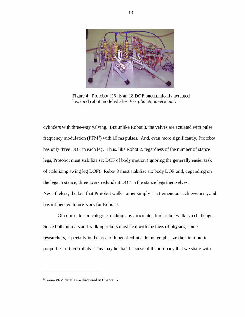
13

cylinders with three-way valving. But unlike Robot 3, the valves are actuated with pulse

frequency modulation (PFM5) with 10 ms pulses. And, even more significantly, Protobot

has only three DOF in each leg. Thus, like Robot 2, regardless of the number of stance

legs, Protobot must stabilize six DOF of body motion (ignoring the generally easier task

of stabilizing swing leg DOF). Robot 3 must stabilize six body DOF and, depending on

the legs in stance, three to six redundant DOF in the stance legs themselves.

Nevertheless, the fact that Protobot walks rather simply is a tremendous achievement, and

has influenced future work for Robot 3.

Of course, to some degree, making any articulated limb robot walk is a challenge.

Since both animals and walking robots must deal with the laws of physics, some

researchers, especially in the area of bipedal robots, do not emphasize the biomimetic

properties of their robots. This may be that, because of the intimacy that we share with

5 Some PFM details are discussed in Chapter 6.

Figure 4: Protobot [26] is an 18 DOF pneumatically actuated hexapod robot modeled after Periplaneta americana.

14

the bipedal system, a certain level of biomimetics is just assumed (whether it exists or

not). This is why biped robots are not listed in the table.

Type 3 and Type 4 robots represent the current state-of-the-art in articulated limb

legged robotics. Not surprisingly, a tension exists between the two areas. Type 4 robots

are costly, complex, and as a result, risky. With these robots, morphological similarity to

the animal has been strongly emphasized. They have the kinematic capacity to move like

the animal, and as a result, these robots look, very much, like the animals they mimic.

That means, almost certainly, that they have more DOF than are necessary to walk. The

cost is the added control complexity needed to move all those joints in a coordinated,

effective, stable manner, which presents a challenge to the roboticist. Yet part of the

aforementioned tension seems to result from a research goal that Type 3 robots do not

share with Type 4 robots (specifically Robot 3). That goal is to have the Type 4 robot

teach the roboticist and the collaborating biologist about the animal and then guide the

biologist’s research. Because of the similar morphologies of the robot and the animal,

these robotic experiences pose specific questions for biologists to examine in the animal’s

locomotion system. These biological experiments in-turn lead to a better understanding

of legged locomotion and, consequently, fundamental progress in legged robotics. The

Biorobotics Lab at CWRU has experienced the benefits of this back-driven research link

many times.

Type 3 robots are actually more closely related to Type 2 robots. The reason is

that, unlike Type 4, Type 3 roboticists deliberately ignore detailed morphology, focusing

instead on functional similarities between their robots and animals [27]. In the case of

the robots listed above, the functional similarity of interest is running. These robots

15

feature abstracted morphology. This means far fewer actuators and DOF (except

Boadicea) than Type 2 robots, some prismatic DOF, and as few sensors as possible, all in

order to keep things as simple as possible. Compared to Type 4 robots, this is a rather

practical approach that can produce immediate short-term results.

RHex [22] is a typical example. RHex is a 15 lb, six-legged robot, where each leg

is a single compliant spoke driven by a motor at the hip. The motor, under PD control,

swings this spoke in a full circle parallel to the sagittal plane of the robot. It is not

difficult to envision control schemes that would immediately produce stable tripod

walking in a short amount of time. (In fact, both the standard and simplified versions of

the biologically inspired Robot 2 controller, which is based on Cruse coordination

mechanisms (see Appendix), should work very well for RHex. The simplified version,

that being the two leg case, was successfully deployed on the K2T robot [4].) In the

same way, it is not difficult to envision the open-loop, yet robust, rough terrain

capabilities of RHex, which have been amply demonstrated. Thus, although RHex is a

simple, reliable, abstract hexapod robot that is easily controlled, its yield in terms of

expanding the knowledge-base of legged robotics beyond Type 2 (except, possibly, in the

in-progress goal area of running) is limited. For instance, RHex’s leg trajectories relative

to the body are fixed, so that it cannot voluntarily reach out to grip an obstacle or enter a

depression in the terrain, thus limiting research opportunities into more complex control.

Hence, the Type 3 approach can have immediate results with relatively little background

research, but the ultimate payoffs are also limited.

16

It seems that an underlying assumption behind Type 3 research is that the only

remaining frontier of legged robots is inherently robust animal-like running. While

definitely an important goal [29], such an assumption would be narrow, since effective

general locomotion involves a nervous system and is not limited to running. For

instance, since Type 3 robots shun sensors, how do these robots help biologists and

roboticists understand the role of graded force feedback in locomotion? One would think

that animals benefit from the wide range of sensors they possess as they interact with an

unpredictably wide range of terrain and, therefore, legged robot designs would also

ultimately benefit from those designs. Most Type 3 robots basically scurry over the

ground by using open-loop feed-forward control, which is made robust through passive

dynamics as long as the robot does not break. Full [30] points out that cockroaches

appear to do this very thing during rapid running, even over uneven terrain. But larger

running animals, such as cats, certainly do not blindly execute a feed-forward motor

Figure 5: RHex [28] is a typical example of a Type 3 robot. Each leg is a single compliant spoke, driven, at the hip, by a motor under PD control. The spoke swings in a full circle parallel to the sagittal plane of the robot. RHex is a simple and reliable hexapod robot with good rough terrain capabilities.

17

pattern during locomotion over uneven or unknown terrain, and nor do insects, as they

efficiently alter leg trajectory to anticipate barriers that are detected in their paths [31]. It

is probable that these observations on rapidly running cockroaches are a special case

involving near-escape response behavior.

There is no doubt that Robot 3 is one of the most morphologically accurate robots

in the world (consider [32]). It is not abstract. In order to understand the challenge posed

by Type 4 robots, one needs to consider that in animals, the physical morphology is

inextricably linked to the nervous system. But, since detailed neurobiological control

principles are difficult to extract from the animal, a robot built according to observable

morphological data will, one would hope, confront the researcher with a system that must

solve fundamentally animal-like control problems. Holk Cruse remarks [33] that

working with robots that are too simple “may preclude the finding of solutions for the

very task for which brains [and, I would say, nervous systems in general] have been

developed [or designed] to deal with.” In attempting to get a Type 4 robot going, the

researcher must develop control hypotheses and test them. The results of these

experiments are valuable for legged robotic research and for legged animal locomotion

research.

The greatest pitfall of this more scientific approach is not that the morphology of

Type 4 robots is too similar to the animal model. Type 4 robots are not meant to be, and

simply cannot be, robotic copies of the animal. Instead, they are parallel problems. By

endeavoring to understand the links between real animal morphology and real observed

animal neural control, incredible insight can be gained into better ways of designing robot

systems and controlling them. And, since the robot control system is eminently available,

18

trying experiments on the robot helps to illuminate many aspects of animal structure and

control. As such, the intellectual link between the roboticist and the biologist is essential.

Both are involved in ongoing research challenges and both benefit from the other’s

success and failure, ultimately driving both fields of investigation to answers that might

not be readily achieved independently. Hence, the great risk of Type 4 robots is that

much research is required to develop them and their control systems. However, the even

greater potential benefit to both robotics and biology would seem to mitigate that risk.

In summary, if the goal is to build a near-term vehicle with some of the abstracted

locomotion abilities of animals, the Type 2 and 3 approaches (or even the Whegs

concept) are the best choices. However, if the goal is to develop a legged robot with

many of the remarkable locomotion abilities of a specific animal and/or to understand

locomotion concepts in the animal, the Type 4 approach is the most appropriate. This

approach requires more research, but it also holds the most promise.

Works Cited 1 Gurvinder S. Virk. Technical Task 1: Modularity for CLAWAR machines –

specifications and possible solutions. 2nd International Conference on Climbing and Walking Robots (CLAWAR’99), eds. G.S. Virk, M. Randall, D. Howard, University of Portsmouth, UK, pp. 737-747, September, 1999.

2 John E. Bares and David S. Wettergreen. Dante II: Technical Description, Results, and Lessons Learned. The International Journal of Robotics Research, Vol. 18, No. 7, pp. 621-649, 1999.

3 Gabriel M. Nelson and Roger D. Quinn. A Quasicoordinate Formulation for Dynamic Simulations of Complex Multibody Systems with Constraints. Dynamics and Control of Structures in Space III, eds. C.L. Kirk, D.J. Inman, Computational Mechanics Publications, Southampton, UK, 1996.

19

4 W. Clay Flannigan, Gabriel M. Nelson, and Roger D. Quinn. Locomotion Controller

for a Crab-like Robot. In Proceedings of the 1998 IEEE International Conference on Robotics and Automation (ICRA'98), Leuven, Belgium, May, 1998.

5 Roger D. Quinn, Gabriel M. Nelson, Richard J. Bachmann, Daniel A. Kingsley, John T. Offi, and Roy E. Ritzmann. Insect designs for improved robot mobility. 4th International Conference on Climbing and Walking Robots (CLAWAR’01), eds. K. Berns, R. Dillmann, Karlsruhe, Germany, pp. 69-76, September, 2001.

6 D.S. Cooke, N.D. Hewer, T.S. White, S. Galt, B.L. Luk, and J. Hammond. Implementation of modularity in Robug IV. 1st International Conference on Climbing and Walking Robots (CLAWAR’98), Brussels, Belgium, pp. 185-191, November, 1998.

7 C. Angle. Genghis: A Six-Legged Autonomous Walking Robot. SB Thesis, Massachusetts Institute of Technology, Cambridge, MA, 1989.

8 C. Ferrell. Robust Agent Control of an Autonomous Robot with Many Sensors and Actuators. Master’s Thesis, Massachusetts Institute of Technology, Cambridge, MA, 1993.

9 Ken S. Espenschied. Biologically-Inspired Control of an Insect-like Hexapod Robot on Rough Terrain. Ph.D. Thesis, Case Western Reserve University, Cleveland, OH, August, 1994.

10 K. Berns, V. Kepplin, R. Müller, and M. Schmalenbach. Airbug - insect-like machine actuated by fluidic muscle. 4th International Conference on Climbing and Walking Robots (CLAWAR’01), eds. K. Berns, R. Dillmann, Karlsruhe, Germany, pp. 69-76, September, 2001.

11 Fred Delcomyn and Mark E. Nelson. Architectures for a biomimetic hexapod robot. Robotics and Autonomous Systems, Vol. 30, pp. 5-15, 2000.

12 H. Kimura, I. Shimoyama and H. Miura. Dynamics in the dynamic walk of a quadruped robot. RSJ, Advanced Robotics, vol.4, no.3, pp.283-301, 1990.

13 R. Spenneberg, and F. Kirchner. Omnidirectional walking in an eight legged robot. In Proceedings of the 2nd International Symposium on Robotics and Automation, pp. 108-114, 2000.

14 F. Pfeiffer, J. Eltze, and J.-J. Weidemann. The TUM-walking machine. Intelligent Automation and Soft Computing, volume 1, pp. 307-323, TSI Press Series, 1995.

15 W. Ilg, K. Berns, M. Deck, and R. Dillmann. Biologically inspired construction and control architecture for a quadruped walking machine. In Proceedings of the European Mechanics Colloquium: Biology and Technology of Walking, Euromech 375, pp. 212-219, Munich, Germany, 1998.

20

16 Shigeo Hirose, Kan Yoneda, Hideyuki Tsukagoshi. TITAN VII: Quadruped Walking

and Manipulating Robot on a Steep Slope. In Proceedings of the International Conference on Robotics and Automation (ICRA’97), Albuquerque, New Mexico, pp. 494-500, 1997.

17 K. Berns. Technical task 3: Operational Environments - Specification for Robots. 2nd International Conference on Climbing and Walking Robots (CLAWAR’99), eds. G.S. Virk, M. Randall, D. Howard, University of Portsmouth, UK, pp. 763–772, 1999.

18 H. Kimura, Y. Fukuoka, Y. Hada, and K. Takasa. Three-dimensional adaptive dynamic walking of a quadruped robot by using neural system model. 4th International Conference on Climbing and Walking Robots (CLAWAR’01), eds. K. Berns, R. Dillmann, Karlsruhe, Germany, pp. 97-104, September, 2001.

19 J. Ayers, P. Zavracky, N. McGruer, D. Massa, V. Vorus, R. Mukherjee, and S. Currie. A Modular Behavioral-Based Architecture for Biomimetic Autonomous Underwater Robots. In Proceedings of the Autonomous Vehicles in Mine Countermeasures Symposium, Naval Postgraduate School, Monterey, CA, pp. 15-31, 1998.

20 D. Papadopoulos and M. Buehler. Stable Running in a Quadraped Robot with Compliant Legs. In Proceedings of the 2000 IEEE International Conference on Robotics and Automation (ICRA’00), San Francisco, CA, April, 2000.

21 Michael B. Binnard. Design of a Small Pneumatic Walking Robot. Master’s Thesis, Massachusetts Institute of Technology, Cambridge, MA, January, 1995.

22 U. Saranli, M. Buehler, and D.E. Koditschek. RHex: A Simple and Highly Mobile Hexapod Robot. The International Journal of Robotics Research, 20(7):616-631, July, 2001.

23 J.E. Clark, J.G. Cham, S.E. Bailey, E.M. Froehlich, P.K. Nahata, R.J. Full, M.R. Cutkosky. Biomimetic Design and Fabrication of a Hexapod Running Robot. In Proceedings of the 2001 IEEE International Conference on Robotics and Automation (ICRA’01), Seoul, Korea, May, 2001.

24 Peter Dilworth. Peter Dilworth’s Home Page. Online: http://www.ai.mit.edu/people/ chunks/chunks.html.

25 S.T. Davis and D.G. Caldwell. The bio-mimetic design of a robot primate using pneumatic muscle actuators. 4th International Conference on Climbing and Walking Robots (CLAWAR’01), eds. K. Berns, R. Dillmann, Karlsruhe, Germany, pp. 197-204, September, 2001.

26 UIUC Hexapod Project. Online: http://soma.npa.uiuc.edu/labs/nelson/hexapod.html.

21

27 R.J. Full and D.E. Koditschek. Templates and Anchors: Neuromechanical Hypotheses

of Legged Locomotion on Land. The Journal of Experimental Biology, Vol. 202, pp. 3325-3332, 1999.

28 The ARL Robots. Online: http://www.cim.mcgill.ca/~arlweb/.

29 M.H. Raibert. Legged Robots that Balance. MIT Press, Cambridge, MA, 1986.

30 R.J. Full, K. Autumn, J.I. Chung, A. Ahn. Rapid negotiation of rough terrain by the death-head cockroach. American Zoologist, 38:81A, 1998.

31 J.T. Watson, R. E. Ritzmann, S. N. Zill and A. J. Pollack. Control of obstacle climbing in the cockroach, Blaberus discoidalis I. Kinematics. J. Comp. Physiol. A, 188:39-53, 2002.

32 Fred Delcoymn. Walking Robots and the Central and Peripheral Control of Locomotion in Insects. Autonomous Robots, Vol. 7, pp. 259-270, 1999.

33 Holk Cruse. Building Robots with a Complex Motor System to Understand Cognition. In Biorobotics: Methods and Applications, eds. Barbara Webb and Thomas R. Consi, AAAI Press, Menlo Park, CA, p. 120, 2001.

22

Chapter 3

Posture Control 6

As legged robots become more animal-like, it is likely that these robots will have

many complex limbs with redundant DOF. This is especially true when we desire them

to move like an animal. Animals are capable of spontaneous and non-stereotyped

locomotion, such as turning, swaying, twisting, deliberately falling, jumping, climbing,

and running. Therefore, it becomes difficult to provide joint space trajectories, in real-

time, for these complex movements when many limbs are simultaneously involved, and

when some or all of these limbs contain redundant DOF. When locomotion takes place

rapidly, it has been suggested that there is a feed-forward control component that

involves a proactive, higher level computation in the nervous system [1].

With this controller, I suggest and demonstrate an intuitive and computationally

efficient algorithm for controlling the posture of a complex, multi-leg robot with many

redundant DOF [2]. The algorithm ignores inverse kinematics, controlling the position of

the body by issuing feed-forward force commands to both maintain static posture and

generate body motion. In so doing, it is also shown that the multi-leg mechanics of

postural control can be reduced to a straightforward center-of-pressure representation, or

equivalently, an instantaneous virtual leg model. The force output of the cylinders can be

6 This section is adapted from [2].

23

approximated by a sigmoidal function of duty cycle, with piston-face area and supply

pressure parameters. This is discussed in more detail in the next chapter.

Robot 2 [3] was loosely inspired by the stick insect but had three degrees of

freedom in each of its six legs. Its joints were driven by DC motors using proportional

position control with adjustable gains. The robot could walk in a continuum of insect-

like gaits and traverse irregular terrain using an insect-based distributed controller.

Posture control was achieved by a mixture of processes local to joints and legs and two

global algorithms. The first global algorithm compared an estimated individual leg load

to the average across all legs, and incremented the desired foot position to help equalize

load among legs. The second monitored body orientation by averaging shoulder

positions and adjusting desired foot set-points to conform the body to overall terrain

orientation as represented by the feet.

With Robot 3, I am defining posture control as the active and continuous

maintenance of body stability in all regimes of locomotion. These regimes include

standing, walking, and running. In ongoing research in physiology, wherein researchers

are seeking to understand how control responsibility for posture and locomotion is

distributed throughout the nervous system, one aspect that is clear is the importance of

higher centers of the nervous system for normal posture. This suggests that posture

control is more than local reflex interaction. It is the orchestration and tuning of these

reflexes according to some central desired behavior. Horak and Macpherson write in the

Handbook of Physiology [4],

Posture is no longer considered simply as the summation of static reflexes but, rather, the complex interaction of sensorimotor processes and internal

24

representations of those processes. Postural orientation involves active control of joint stiffnesses and such global variables as trunk and head alignment, based on the interpretation of convergent sensory information. Postural equilibrium involves coordination of efficient sensorimotor strategies to control the many degrees of freedom for stabilization of the body’s center of mass during either unexpected or voluntary disturbances of stability.

Although investigated in different contexts and by various researchers, the

approach to posture control for Robot 3 was inspired by the Virtual Model control

scheme as presented by Pratt et al. [5]. Contributing research fields are also described

well by Pratt [6]. A description of this scheme is discussed in the following sections. Lin

and Quinn [7] used the inverse of this approach in a dynamic simulation of Robot 2. This

chapter proposes an internal model tailored to the locomotion needs of a system such as

Robot 3. The concepts represented by this model are by no means new [8, 9], but one

goal of this work is to demonstrate the successful implementation of these ideas into a

complex, animal-like robot.

25

3.1 Single Leg Mechanics

Consider what contribution a single limb has on force production at the body of

the robot. The system consists of the main body with its own fixed reference frame (1-

frame), and a sequential numbering of leg segments out to the foot, each with its own

body-fixed reference frame (2, 3, etc. -frames). The main body reference frame can be

located at (but not restricted to) what can be considered an average center of mass (CM)

position. (This is a static position. It does not require a calculation of instantaneous CM

location.) The segments are connected with rotary joints only. In this application, we

assume that the leg maintains a point contact with the ground, producing an “unactuated

zN

yN

xN

y1

x1

z1

body 1

body 2

body 3

body 4

x1 ≡ longitudinal (direction of travel)y1 ≡ lateral (left)z1 ≡ vertical

W2L2

L1

Figure 6: Single leg mechanics notation. The body reference frame consists of the x1 ≡ rostral or direction of travel, y1 ≡ lateral or left, z1 ≡ vertical. Each body (1 through 4) contains its own body-fixed reference frame. The vector definitions (Li and Wi) are given in the text.

26

ankle” constraint. This generates a required relationship between the forces and moments

applied by the leg, l, on the body,

lllll FJFC}W{M N11 == , l = i, ii, …, d, (1)

where Fl and Ml are force and moment vectors, respectively, applied at the body’s

reference frame. d represents the number of legs in contact with the ground at this time.

Fl is expressed with respect to an inertial reference frame (N-frame) while Ml is

expressed with respect to the body (1-frame). W1l is the position of the foot of leg l in

the body’s reference frame, and {W} represents a skew operation on a vector,

−−

−=

0WWW0W

WW0}W{

xy

xz

yz

(2)

C1N is a 3x3 rotational transformation matrix from the inertial frame to the body frame.

A recursive set of W vectors for a leg with two segments can be expressed as follows:

21211 WCLW +=

32322 WCLW +=

33 LW = (3)

where each vector Li represents the position of the next distal (i+1) body-fixed reference

frame in the i-frame (typically located at the next joint), each vector being expressed with

respect to the i-frame (see Figure 6). Thus, the transpose Jacobian for a given leg with

m-1 segments is expressed as

=

mNm

N33

N22

TT

C}W{

C}W{

C}W{

DJM

, (4)

where D is a matrix describing the specific joint geometries [10].

27

3.2 Somatosensory Feedback of Body Position

Somatosensory feedback has its origin outside central sensory organs, such as are

found in visual or vestibular systems. It comes from distributed sensory information that

reflects physical contact of the body with the environment. For both robustness and

simplicity, Robot 3 (and Robot 2 [11]) does not rely on any single sensory device for

determining body position. Unlike other robots with fewer legs, it is possible to estimate

this information from the three or more simultaneous stance legs.

Using a least squares approximation, a support surface plane is estimated from the

positions of the stance feet. This calculation produces an estimate for C1N which

excludes any yaw component. The height of the robot is estimated by averaging the

opposite of the vertical (z) locations of the feet. Determining a yaw angle, as well as the

horizontal (x and y) location of the body requires a convention, since somatosensory data

will contain no absolute information about the orientation of the body relative to the

ground along these axes. This is further complicated when legs are not in stance.

Preliminary results indicate that it is sufficient to simply average the x, y, and yaw

locations of all the feet, regardless of state, to arrive at a suitable reflection of body

location. Sensing the orientation of gravity is external to this calculation. It would

involve the use of an inclinometer and/or force data. Cockroaches, having no single

sensor for detecting gravity, appear to use convergent force data from the exoskeleton.

For the sake of this discussion, I will assume that gravity acts solely in the vertical,

negative z direction.

28

3.3 Multi-leg Mechanics

All stance legs act on the body of the robot in parallel. Considering an arbitrary

case in which four legs (d = 4) are in stance we have,

=

MF

F

FF

F

JJJJIIII

iv

iii

ii

i

iviiiiii,

[ ]zyxT FFFF = ,

[ ]zyxT MMMM = ,

(5)

where F and M (no subscript) represent the combined action of all stance legs on the

body. lJ is defined implicitly in Eq.(1), and I is the identity matrix. The goal is to

specify virtual forces, F and M, using an appropriate and capable virtual model (hence the

name “Virtual Model”), and then to solve for the individual leg forces, Fl, that would

tend to produce these virtual forces. This is not a trivial problem, and has received much

attention in several decades of research. To specify F and M, we could simply drive the

position of the body using imaginary actuators (of our choice) following desired

behaviors. In controlling a planar biped robot, Pratt et al. used intuitive actuators like a

linear damper, between the body and a moving target (a “dog-track bunny”), to control

forward speed, and a spring arrangement, between the body and the ground (a “granny

walker”), to control body height and attitude [5]. Choosing these model actuators is

29

beautifully open-ended, yet is limited by, among other things, the amount and quality of

sensory information available to the robot.

3.4 Solving the Force Distribution Problem

At least three methods have been used to solve the redundancy problem presented

by Eq. (5). The first method entails using additional constraints to create a square and

(hopefully) invertible coefficient matrix to immediately solve for the local leg forces.

The second involves pseudoinverses that provide some desirable qualities (such as

preservation of configuration after a cycle of motion [12]). Related to this, the third

method involves using optimization functions that portray some desirable behavior (i.e.

minimize joint torques or force distribution [13], base reactions [14], joint motions,

kinetic energy). Optimization has been used for the control of redundant manipulators

for many years [15, 16].

The approach taken in this thesis borrows from the third of these techniques. The

additional constraint method was investigated, but generally suffered from singularities

that depended on the kinematic state of the system. The foremost of these singularities,

which is discussed below, can be used to significantly simplify the force distribution

problem and introduce an intuitive center-of-pressure representation. This, in turn,

allows the stance mechanics to be divided into vertical and horizontal optimization

problems. The resulting algorithm is consistent regardless of the number of legs

simultaneously contacting the ground.

30

We begin by introducing some dimensionless parameters. Let each leg, l, assume

a vertical load responsibility coefficient nl, 0 ≤ nl ≤ 1,

z

z

FF

n ll = , 1n =∑

ll , l = i, ii, iii, iv. (6)

Also, let the direction in which each leg pushes be described by two other dimensionless

coefficients,

l

ll

z

xx F

Fc = ,

l

ll

z

yy F

Fc = . (7)

Eq. (5), reduced from six to five rows by the introduction of Eqs. (6), can be

expressed in terms of these coefficients,

F

c

cc

cc

cc

c

nnnnnnnn

n0n0n0n00n0n0n0n

yiv

xiv

yiii

xiii

yii

xii

yi

xi

2iv

1iv

2iii

1iii

2ii

1ii

2i

1i

iviiiiii

iviiiiii

=

(8)

where

kk Jnn lll = , thk kJ ≡l column of lJ , (9)

and

+++−

=

=3iv

3iii

3ii

3i

z

y

x

y

x

z

5

4

3

2

1

nnnn

00

MMMFF

F1

FFFFF

F (10)

31

The characteristics of the five scalar equations in Eq. (8) prove useful for simplifying this

problem. Denoting the position of the foot relative to the body, expressed with respect to

the N-frame, as

l

l

l

l

l 11Nfoot WCzyx

p =

= , (11)

we can assume a case in which the body of the robot is coincident with the N-frame

(C1N = I)7, and all of the stance feet are at equal vertical locations, such as standing on a

flat surface (zl = z)8. This causes the first and fourth rows of Eq. (8) to become linearly

dependent,

1xivivxiiiiiixiiiixii Fcncncncn =+++ ,

4xivivxiiiiiixiiiixii F)cncncncn(z =+++ , (12)

as well as the second and third rows of Eq. (8),

2yivivyiiiiiiyiiiiyii Fcncncncn =+++ ,

3yivivyiiiiiiyiiiiyii F)cncncncn(z =+++− . (13)

Note that such a common kinematic configuration (standing straight and level on flat

ground) causes a singularity in attempts to solve the force distribution problem using

arbitrary additional force constraints. This singularity would require that

41 FFz = , 32 FFz =− . (14)

7 This assumption is inconsequential since Eq. (1) can be premultiplied by CN1 to produce the same results

below.

8 When the feet are not at equal zl locations, it is often feasible to approximate by assuming zl = zavg.

32

Although this may seem to be a special case, it lends insight into an underlying model for

the stance mechanics. We can express the location of a center of pressure (abbreviated

COP, sometimes called the Zero Moment Point or ZMP) below the robot as

∑=l

llxnxcop , ∑=l

llynycop . (15)

Thus, we discover that Eqs. (14), when simplified, produce the following relationships:

z

y

z

xcop F

M

FzF

x −= , z

x

z

ycop F

MF

zFy += . (16)

These correspond to a single leg model of the mechanics of the robot, which is shown in

Figure 7. (Note that z is typically negative.)

Mx

COP

z

z

y

z

y

FF

z

x

FM

z

y

F

zF

=

z

y

FF

Figure 7: Single virtual leg model of robot mechanics. Provided with desired virtual forces acting on the body, the posture controller predicts the position of a center of pressure (COP) where a virtual leg would, at that instant, produce those virtual forces. The scheme is repeated for the x-z plane. The virtual leg would also have a foot (not shown) that would produce a desired virtual Mz.

33

To solve for the force distribution, the mechanics described by this single leg

model can be used as a suitable representation of the locomotion of the robot. Once the

components of the virtual forces, F and M, are chosen, we can determine a desired COP

position directly from Eqs. (16). Locating the COP as such satisfies the singularity and

allows us to drop the third and fourth rows of Eq. (8). This is equivalent to achieving the

instantaneous, virtual presence of the single leg model shown in Figure 7. Ting et al. [17]

partially describe solving the forward version of this problem for measured foot force

data from an actual cockroach, referring to a “single effective leg”. Their informal

approach implies Eq. (16) to find a COP from the data, but they neglect to account for

Mz. Schmitt et al. [18] also point this out.

By choosing an intuitive function to minimize,

−= ∑l

ll2*

n )nn(21

E , (17)

and remembering the three constraints of Eqs. (6) and (15), we can solve for the weight

distribution across the robot’s legs. *nl represents a desired vertical load responsibility

for each leg, usually set to 1/d. Once all nl are known, the rectangular matrix and right

side of Eq. (8) are known. Based upon biological observations [19], we know that

cockroaches produce forces in directions related to the attitude of each leg (although this

is obviously task and context dependent). Viewing the first, second, and fifth rows of Eq.

(8) as constraints, we can introduce another cost function,

∆+∆= ∑l

ll )cc(21

E 2y

2xc , (18)

where

34

*xxx ccc lll −=∆ , *

yyy ccc lll −=∆ . (19)

Minimizing Ec will encourage, but not enforce, each leg to push in a preferred, animal-

like direction. *xc l and *

yc l are determined by minimizing joint torques in the leg l. (The

form of Ec was chosen for computational efficiency. Other more isometric functions

could be used.)

3.5 Results

This algorithm has been successfully implemented, and is able to control the

standing posture of Robot 3 in the presence of disturbances, as well as respond to

commanded body positions and orientations.

The following two figures describe a test in which the robot was pushed while

standing. These disturbances amounted to the operator standing to the right of the robot

and vigorously shoving the robot to its left with both hands [20]. In some cases the robot

was perturbed with a single hand in the abdomen or head areas. As a reference for the

following figures, these perturbations from the robot’s right side caused it to sway in the

lateral, or y, direction. Virtual springs, attached to the body reference frame, cause the

robot to maintain a standing position.

35

25 30 35 40 45 50 55

Time (secs)

-1

0

1

2

3

y (in)

disturbance

y pos

y cop

Figure 8: Disturbance rejection while standing via posture control. While standing, the robot was shoved repeatedly. Each arrow indicates a disturbance. The robot swayed and returned to a nominal standing position. “y pos” indicates the y, or lateral, position (see Figure 6) of the body. “y cop” is the y location of the COP. The COP moved to counteract the disturbances. The COP was slightly negative because the robot perceived a small roll error (lean to left). Stiction in the cylinders caused the initial and final body positions to be slightly different.

25 30 35 40 45 50 55

Time (secs)

00.10.20.30.40.50.60.70.80.9

1

n (%)

left n

right n

Figure 9: Vertical load transfer to move COP. Corresponding to Figure 8, this figure shows how vertical load responsibility was transferred to the left side legs as the COP moves to counteract the disturbances. “left/right n” is the ipsilateral sum of nl values.

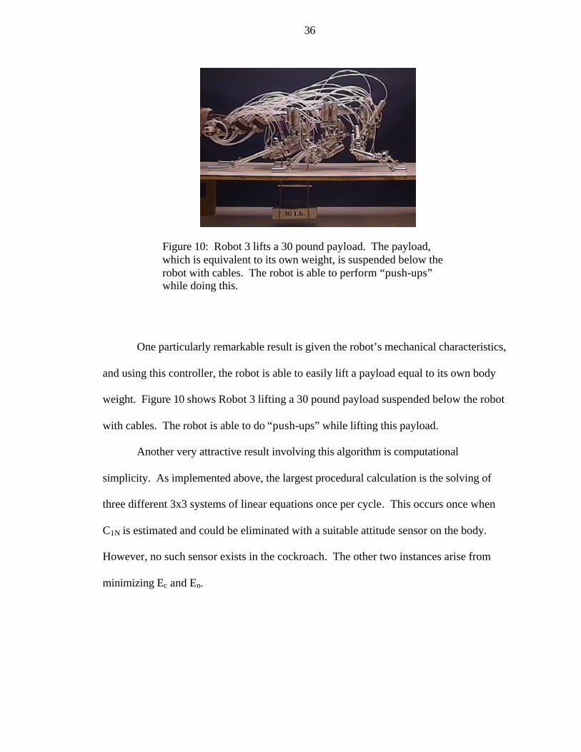
36

One particularly remarkable result is given the robot’s mechanical characteristics,

and using this controller, the robot is able to easily lift a payload equal to its own body

weight. Figure 10 shows Robot 3 lifting a 30 pound payload suspended below the robot

with cables. The robot is able to do “push-ups” while lifting this payload.

Another very attractive result involving this algorithm is computational

simplicity. As implemented above, the largest procedural calculation is the solving of

three different 3x3 systems of linear equations once per cycle. This occurs once when

C1N is estimated and could be eliminated with a suitable attitude sensor on the body.

However, no such sensor exists in the cockroach. The other two instances arise from

minimizing Ec and En.

Figure 10: Robot 3 lifts a 30 pound payload. The payload, which is equivalent to its own weight, is suspended below the robot with cables. The robot is able to perform “push-ups” while doing this.

37

3.6 Conclusions

As shown above, the force distribution problem for a multi-legged system such as

Robot 3 has already embedded within it a single leg model that intuitively describes the

mechanics. This model is derived mathematically, yet is intuitive and connects well with

previous observations by both biologists and roboticists [21]. It is central in solving the

redundancy problem and produces a computationally efficient algorithm for controlling

posture during locomotion.

The posture controller unifies the two separate posture control algorithms used for

Robot 2. The Robot 3 posture control does not address or control individual foot

positions, but rather a general sense of body position as described by these foot positions,

whatever they may be. Thus, when setting Robot 3 on uneven terrain, the legs will

automatically comply to surface irregularities while the robot automatically controls body

position to an average height and average terrain orientation. The vertical loading at each

foot is automatically adjusted to realize the desired COP, which is a direct function of the

virtual forces acting on the body that themselves come from virtual actuators that

promote proper posture.

Another way of understanding the Robot 3 posture control is to consider the joint

set-point positions that Robot 2 attempted to follow in order to stand and walk. These

positions represent a reference Robot 2 that moved in a significantly different

configuration than the actual robot. Espenschied remarked [22] that a seemingly more

insect-like (vertical) posture control scheme would be to lower the stiffnesses (position

control loop gains) of the main load bearing motors and then move the corresponding

38

joint set-points further away to compensate. This is, in effect, how Robot 2 operated.

The robot would attempt to follow a reference robot that, kinematically, was significantly

hyper-extended, and that it really had no intention of actually tracking. This is obvious

since tracking errors, which reflect the postural loads themselves, need to be generated.

The Robot 3 posture controller is that piece of the Robot 3 “brain” that directly predicts

and generates these loads, and not just for vertical posture. Because of the significantly

slower actuators used on Robot 3, high gain local position control is difficult, if not

impossible, to realize (see Chapters 6 and 7), and the need for this type of posture control

makes sense. The posture controller defines an overall force production plan or profile

for all the actuators involved in stance, and local feedback pathways slightly or

moderately modify this profile based on local kinematic and load feedback. As a result,

these local control loops (i.e. position control of a joint) would be able to operate at lower

gains or stiffnesses because the posture control has already provided intelligent offsets

that effectively represent the current locomotion of the robot. Thus, the goal now

becomes addressing the local kinematics that the posture controller essentially ignores.

This is the topic of Chapter 5.

Central to this posture control strategy is the transcending physical description

represented by Eqs. (16). These equations tell us several things. (i) The horizontal and

vertical posture control mechanics are directly linked. Or more specifically, (ii) actuators

involved in producing primarily vertical forces are extremely important (indeed, possibly

dominant) in horizontal posture control (which, in my definition of “posture control”

applies to all general locomotion). Also (iii) the choice of virtual actuators, which

produce the virtual forces and moments on the body, is directly linked to the support

39

polygon and where the robot can produce a COP. This has significant implications for

biped control [23].

Works Cited 1 A. Prochazka. Proprioceptive feedback and movement regulation. Handbook of

Physiology, section 12, eds. L. Rowell and J.T. Shepherd, assoc. ed. J.L. Smith, pp. 89-127, 1996.

2 G. M. Nelson and R. D. Quinn. Posture Control of a Cockroach-like Robot. IEEE Control Systems, Vol. 19, No. 2, April 1999.

3 K.S. Espenschied, R.D. Quinn, H.J. Chiel, and R. Beer. Biologically-based distributed control and local reflexes improve rough terrain locomotion in a hexapod robot. Robotics and Autonomous Systems, Vol. 18, pp. 59-64, 1996.

4 F.B. Horak and J.M. Macpherson. Postural orientation and equilibrium. Handbook of Physiology, section 12, eds. L. Rowell and J.T. Shepherd, assoc. ed. J.L. Smith, pp. 255-292, 1996.

5 J. Pratt, P. Dilworth, and G. Pratt. Virtual model control of a bipedal walking robot. In Proceedings of the 1997 IEEE International Conference on Robotics and Automation (ICRA’97), Albuquerque, New Mexico, 1997.

6 J. Pratt. Virtual model control of a biped walking robot. Master’s Thesis, Massachusetts Institute of Technology, Cambridge, MA, August, 1995.

7 R.D. Quinn and N.J. Lin. Dynamics and simulation of an insect-like hexapod robot. In Proceedings of the 9th VPI&SU/AIAA Symposium on Dynamics and Control of Large Structures, May, 1993.

8 M.H. Raibert, M. Chepponis, and H.B. Brown, Jr. Running on four legs as though they were one. IEEE Journal of Robotics and Automation, Vol. RA-2, No. 2, pp. 70-82, June, 1986.

9 R. Blickhan, R.J. Full. Similarity in multilegged locomotion: Bouncing like a monopode. J of Comp. Phys. A, 173:509-517, 1993.

10 Gabriel M. Nelson and Roger D. Quinn. A Quasicoordinate Formulation for Dynamic Simulations of Complex Multibody Systems with Constraints. Dynamics and Control of Structures in Space III, eds. C.L. Kirk, D.J. Inman, Computational Mechanics Publications, Southampton, UK, 1996.

11 Ken S. Espenschied. Biologically-Inspired Control of an Insect-like Hexapod Robot on Rough Terrain. Ph.D. Thesis, Case Western Reserve University, Cleveland, OH, August, 1994.

40

12 F.A. Mussa-Ivaldi, N. Hogan. Integrable Solutions of Kinematic Redundancy via

Impedance Control. Int. J. of Robotics Research, Vol. 10, No. 5, pp. 481-491, October, 1991.

13 F. Pfeiffer, H.-J. Weidemann, P. Danowski. Dynamics of the Walking Stick Insect. In Proceedings of the 1990 IEEE International Conference on Robotics and Automation, Cincinnati, Ohio, 1990.

14 R.D. Quinn, J.L. Chen, C. Lawrence. Base Reaction Control for Space Based Robots Operating in a Microgravity Environment. AIAA J. of Guid., Cont., & Dyn., Vol. 17, No. 2, pp.263-270, 1994.

15 D. Schmitt, A.H. Soni, V. Sirivasan, G. Naganathan. Optimal Motion Programming of Robot Manipulators. ASME J. of Mechan., Trans. and Automat. in Design, Vol. 107, pp. 239-244, June 1985.

16 N.J. Lin, R.D. Quinn. The Use of Locally Optimal Trajectory Management for Base Reaction Control of Robots in a Microgravity Environment. Proc. of the 1991 AIAA Guid., Nav., and Cont. Conf., New Orleans, Aug., 1991.

17 L.H. Ting, R. Blickhan, and R.J. Full. Dynamic and Static Stability in Hexapedal Runners. Journal of Experimental Biology, 197:251-269, 1994.

18 J. Schmitt, P. Holmes. Mechanical models for insect locomotion: dynamics and stability in the horizontal plane I. Theory. Biological Cybernetics, 83:501-515, 2000.

19 R.J. Full. Integration of Individual Leg Dynamics with Whole Body Movement in Arthropod Locomotion. In R.D. Beer, R.E. Ritzmann, and T. McKenna (eds.), Biological Neural Networks in Invertebrate Neuroethology and Robotics, Academic Press: NewYork, 1993.

20 G.M. Nelson, R.J. Bachmann, R.D. Quinn, J.T. Watson, R.E. Ritzmann. Posture Control of a Cockroach-like Robot (Video). Video Proc. Of the 1998 IEEE Int. Conf. on Robot. and Automat., Leuven, Belgium, 1998. (Online: http://biorobots.cwru.edu/ Projects/robot3/robot3.htm)

21 I.E. Sutherland, M.K. Ullner. Footprints in the asphalt. Int. J. of Robotics Research, Vol. 3, No. 2, pp. 29-36, 1984.

22 Ken S. Espenschied. Biologically-Inspired Control of an Insect-like Hexapod Robot on Rough Terrain. Ph.D. Thesis, Case Western Reserve University, Cleveland, OH, pp. 90-91, August, 1994.

23 K. Sari, G.M. Nelson, and R.D. Quinn. Dynamics and Control of a Simulated 3-D Humanoid Biped. Int. Symposium on Adaptive Motion of Animals and Machines (AMAM), Montreal, Quebec, Canada, August 8-12, 2000.

41

Chapter 4

Posture Control Implementation Issues

In this chapter, I discuss some of the implementation issues affecting the

performance of the posture control of Chapter 3.

4.1 Original Hardware Setup

The overall original posture control hardware setup followed the scheme depicted

PC#1

PostureController

PC#2

PWM

Robot 3

sensorinformation

valvecommands

commandedduty cycles

Figure 11: The overall original posture control system. Computer #2 (PC#2), which was slaved to computer #1 (PC#1), performed PWM on the 48 valves at a frequency of 50 Hz according to commanded duty cycles from PC#1. PC#1, directly reading sensory information from the physical robot, performed posture control calculations and output commanded duty cycles to PC#2.

42

in Figure 11. This triangular configuration is actually optimized for pure posture control,

since PC#2 is simply an efferent extension of the physical robot and afferent information

comes directly back to the posture controller. Thus, the posture controller needn’t work

through a secondary, or lower-level, controller to access the robot.

Figure 12 unpacks the details of Figure 11. Using DOS as the computer operating

systems for the controllers is certainly not cutting edge, mainly (in my opinion) due to the

lack of interface. Yet DOS (with clever programming) is a pliable tool that can be made

sufficiently single-minded in order to achieve the time-critical execution needed, for

instance, to perform PWM. For future robots, I have actively endorsed a transition to

real-time Linux. The system depicted in Figure 12 did operate correctly and to

RS

232

PWM

serialcable

OptoOpto

OptoOpto

OptoOpto

Valves

Air

ribboncable

ribboncable

Robot Frame

pots

s.gagesControl

hoses

A/Dribboncable

PC#1 Dell133MHz Pentium

PC#2Gateway127 MHz

AMD

Physical RobotOptos

Figure 12: Original Robot 3 posture control basic electronics. PC#1 was a 133MHz Pentium desktop running the posture controller in DOS. The controller dispatched (unbuffered) commanded duty cycles to PC#2, a 127MHz AMD desktop, via 115200 bps serial communication. PC#1 also read 24 potentiometer signals from an ISA A/D (12 bit) card (original gage signals, which were not used, were one per leg and meant for binary contact sensing only). PC#2, running in DOS, polled a timer card to perform 50 Hz PWM with about a 1% resolution. A digital I/O card drove 48 opto-isolators, which in turn drove the valves of the robot.

43

specification, which was verified with an oscilloscope monitoring various digital out

signals from PC#2.

4.2 Open-loop force control

It should not be overlooked that in order to realize the posture control discussed

above, the control system for Robot 3 must be able to produce desired joint torques with

some reasonable level of fidelity. In fact, the entire Virtual Model Control scheme, as it

is used at the MIT Leg Lab, is born out of the painstaking and very successful

development of Series Elastic Actuators (SEA) [1]. By placing a spring in series between

a motor-driven ball screw and the load, SEA provide good force control with a large

dynamic range and shock tolerance. A linear potentiometer measures the deflection of

the spring, and thus allows for control of the output force. The SEA used by Pratt [2] had

a force control bandwidth of 14 Hz with a (maximum) phase lag of about 65 - 70 degrees

at the cutoff frequency.

Alas, such a hard-earned luxury is not available on Robot 3. At the time of its

implementation, the most the posture controller could hope for was an open-loop

relationship relating desired cylinder force to commanded duty cycle. A simple test stand

was built that used a four pound scale and a 24½:1 reduction to measure the steady-state

force output of a pneumatic cylinder driven with 50 Hz PWM. Supply air pressure was

100 psig. A few tests on cylinders of different diameters indicated the relationship shown

in Figure 13.

44

Two different sized cylinders were tested at two separate stroke lengths. The

force outputs were then normalized by their theoretical maximums. The curve fit

equation, as a function of commanded duty cycle, 0 ≤ D ≤ 100, was

13.0

e103.1

FF

F D1.03.4max

−+

== − , (20)

which, when inverted, becomes

0 10 20 30 40 50 60 70 80 90 100

0.5

0.4

0.3

0.2

0.1

0

-0.1

-0.2

0.8

0.9

1

0.7

0.6

Command duty cycle

NormalizedforceF/Fmax

Figure 13: Original duty cycle to force output relationship at 50 Hz PWM. Various cylinder sizes were tested for their steady-state force output as a function of duty cycle at 50 Hz PWM. The curves were then normalized by the theoretical maximum force for that cylinder size, and a sigmoidal curve was fit to the data (Eq. (20)). The inverse of this relationship was used for open-loop force control.

45

−

+−= 1

13.0F03.1

log1043D e . (21)

Obviously, Eqs. (20) and (21) are only used for F ≥ 0. The result of the posture control

calculations is a desired joint torque that is converted into a desired cylinder force while

accounting for that joint’s transmission linkage kinematics [3]. This desired force is

normalized by the flexor or extensor dimensions of that cylinder9, and converted into a

duty cycle with Eq. (21). Notice that commanded duty cycles below about 23% simply

produce no force output from the actuator. Also, notice the small region above 95% duty

cycle where the forces climb more steeply. Both of these features are fundamental

electromechanical properties of the valve, which will be discussed in Chapter 6.

Eq. (21) was used across all joints of Robot 3 in the Posture Control video

featured at the 1998 IEEE International Conference on Robotics and Automation (ICRA)

[4]. As the video clearly demonstrates, the posture controller works extremely well. In

fact, it is remarkable that the open-loop force control works as well as it does, especially

during the commanded body motions shown in the video. Clearly, something about this

scheme was “on-track”.

But there were some hidden problems. First and foremost, it was hoped that with

the posture controller maintaining body attitude (height, lateral position, and orientation)

while simultaneously following a forward-moving attractor (to generate forward

propulsion), Cruse rules [5] could be used to coordinate the legs for successful walking.

To handle the changes in loading caused by leg switches from stance to swing and vice

versa, transitioning legs could be selectively merged in to and out of the optimization

9 For a table of cylinder sizes on Robot 3, see [2]

46

calculation of Eq. (17). This is done by simply removing that leg from the optimization

and directly assigning its load responsibility coefficient, nl. Unloading legs followed a

rapidly decreasing nl to zero, while loading legs rapidly ramped up a target responsibility

continuously calculated by the posture control.

The outcome, though, was not acceptable walking. Although the posture

controller kept the robot standing, the reliability of the postural maintenance during

transitions was poor. The ensuing locomotion was more pitiable stumbling than any sort

of recognizable walking, often closely resembling the first meager steps of a newborn

colt or calf.

During investigations, I noticed that at least one of the legs, the right middle leg,

was supporting relatively little weight compared to its neighbors. A quick check revealed

the problem: the performance of some valves was considerably different (up to 40% off)

than the assumed open-loop relationship of Eq. (20). In the previous posture results,

these errors in joint loading in the right middle leg had simply been masked by the better

performance of its neighboring legs, especially while all six legs were supporting weight.

Obviously, during walking attempts, this poor performance was revealed since the

posture control must rely more heavily on proper performance from individual legs while

other legs are in swing. The result of this investigation was the creation of individual

“valve curves” (such as Eq. (21)) or look-up tables for the 48 valves on Robot 3. These

tables were created in the same way that the data for Eq. (20) were collected.

47

4.3 Conclusion

Despite the new valve curves, there were only minor, yet noticeable,

improvements in the walking performance of the robot. It was becoming clear, as

biology would suggest, that posture control, with gait coordination, is not enough to

generate acceptable walking. The posture control scheme was not involving itself in any

of the following: muscle-like actuator properties (either passive or emulated), local

stretch reflex pathways, and load feedback. Clearly, well-known mechanisms in the

neural control of movement were being ignored.

On the positive side, though, the posture controller was keeping the robot upright

and standing, which was something initial tests with just local joint control failed at

immediately. Obviously, the posture control was a foundation upon which to build more

independent feedback control pathways, which is the topic of the following chapters.

Works Cited 1 G.A. Pratt and M.M. Williamson. Series Elastic Actuators. In Proceedings of the

IEEE International Conference on Intelligent Robots and Systems 1, pp. 399-406, 1995.

2 J.E. Pratt. Exploiting Inherent Robustness and Natural Dynamics in the Control of Bipedal Walking Robots. Ph.D. Thesis, Massachusetts Institute of Technology, Cambridge, MA, June, 2000.

3 Richard J. Bachmann. A Cockroach-like Hexapod Robot for Running and Climbing. Master’s Thesis, Case Western Reserve University, Cleveland, OH, May, 2000.

4 G.M. Nelson, R.J. Bachmann, R.D. Quinn, J.T. Watson, R.E. Ritzmann. Posture Control of a Cockroach-like Robot (Video). Video Proc. Of the 1998 IEEE Int. Conf. on Robot. and Automat., Leuven, Belgium, 1998. (Online: http://biorobots.cwru.edu/ Projects/robot3/robot3.htm)

48

5 H. Cruse. What mechanisms coordinate leg movement in walking arthropods? Trends

in Neural Science, Vol. 13, pp. 15-21, 1990.

49

Chapter 5

Inverse kinematics10

The local control discussed in this chapter and the next is simply proportional

position control at the joint level, which is well understood and straightforward to

implement (details of which are discussed in the Chapter 6). The first step is to devise a

way of coming up with desired joint set-points to be followed which is the subject of this

chapter. The following overall notation will be used in this discussion.

5.1 General Notation

10 The following section is adapted from [6].

q vector of joint angles qi ith joint angle qmr vector of midrange joint angles qi+ upper limit of ith joint angle qi- lower limit of ith joint angle Kj joint-space stiffness matrix Kt task-space stiffness matrix Cj joint-space viscous damping matrix pfoot/a actual foot position vector pfoot/d desired foot position vector J Jacobian NJ Nullspace of J JA augmented Jacobian φ(q) “self motion” task function(s) Jφ Jacobian of task function(s) Kφ task function(s) stiffness matrix J* Jacobian pseudoinverse

Ffoot force vector acting on foot τ vector of joint torques WO NN output layer weight matrix WI NN input layer weight matrix

IW′ WI with last column deleted net vector of NN hidden-layer inputs neti ith value of net sig(x) := 1/(1+e-x) dsig(x) := e-x/(1+e-x)2 HLN number of hidden layer neurons t time H( ) Hamiltonian function λ vector of Lagrange multipliers N number of joint-space DOF M number of task-space DOF

50

5.2 Redundant limb kinematics

For legged robots, especially those confronted with complex terrain, limbs having

more controllable joint-space DOF than task-space DOF (i.e. kinematic redundance)

present significant mobility advantages as well as control challenges. To make use of

this added mobility, the well known “ill-posed” inverse kinematics problem must be

addressed. This problem comes from the need to specify more control inputs (i.e. set-

points, gains, forces, etc.) for the joint-space DOF than are required for controlling the

foot (or end effector) DOF of the limb. We can write the forward kinematics equation for

a redundant robot leg, which describes the position of the foot, as

pfoot/a = pfoot/a(q), (22)

where pfoot/a is a M-dimensional vector in task-space, and q is a N-dimensional vector in

joint-space. When N > M, the leg is redundant. The inverse kinematics problem

involves finding a unique inverse function for Eq. (22),

q = q(pfoot/d). (23)

One might obviously choose to “lock-out” or otherwise specify a priori the motion of the

excess DOF, yet this could, and often does, incur an undesirable loss of dexterity.

Specifying “self motion” tasks constraints [1] is a more general and flexible approach of

this type, in which N-M user-defined constraint functions, in terms of q, are used to

resolve the redundancy such as to fulfill certain tasks like avoiding obstacles.

Differential methods based on pseudoinverses of the Jacobian matrix are also often used

as a solution [2, 3, 4]. A common pseudoinverse approach is to minimize joint-space

velocity in a constant weighted fashion. Yet, as several researchers have shown [5],

51

unless special care is taken, constant weight pseudoinverse schemes suffer from

nonintegrability: a closed path in task-space is not guaranteed to produce a closed path in

joint-space. For instance, a leg of a walking robot having redundant DOF may not return

to the same configuration after a cycle of foot motion. In some cases, after many cycles

the configuration trajectory may converge. Then again, it may not.

This prompts a reasonable question. Animal limbs have redundant DOF, yet we

observe (in steady-state behavior) repeatable configurations over many cycles of motion.

One compelling explanation is that animals limbs move in such a way as to minimize the

potential energy stored in the compliance of the actuators (muscles, tendons, etc.). Thus,

assuming that the cyclical limb motion does not enclose any singularities11, the limb

configuration will be a unique function of end effector position, joint set-points and joint

compliance, and therefore repeatable.

The purpose of this section is to discuss the solution of this problem for the legs

of Robot 3 [6]. In this discussion we will isolate on the front legs. The task-space for

these legs is the three-dimensional Cartesian position of the foot relative to the body-coxa

joint of the leg (i.e. the shoulder). This makes the front legs redundant, with five joint-

space DOF (N = 5) and three task-space DOF (M = 3).

11 Or in other words, in a given configuration with the limb moving only quasi-statically, the end effector (a

hand or foot) can be moved a small increment along all task-space DOF without experiencing infinite resistance.

52

5.3 A Practical Goal: Maximize Leg Mobility

The original motivation for the investigation discussed below was the practical

goal of maximizing leg mobility. This involves avoiding joint limits during locomotion,

and redundancy in the front legs of Robot 3 allow for optimization in pursuit of this goal.

One reasonable approach is to achieve desired Cartesian foot locations by using joint

angles that minimize deviations from preferred midrange positions, thus simultaneously

minimizing the chances of encountering joint limits. Mathematically, this problem is

equivalent to minimizing the strain (potential) energy in mechanically conservative

elastic elements (i.e. springs) acting on the joints while driving the foot to desired

Cartesian positions. For simplicity, the spring rates are assumed linear and gravity is

neglected. The equilibrium angles for the springs are set to the midrange joint positions.

This results in the following straightforward constrained optimization:

)pp(qKq),q(H a/footd/footT

jT

21 −λ+∆∆=λ (24)

where ∆q = (q – qmr). Finding the extrema with respect to q and λ, and replacing λ with

Ffoot, results in two conditions:

qKFJ jfoot

T ∆= , where

∂

∂=

qp

J a/foot , (25)

a/footd/foot pp = . (26)

These are the expected conditions: Eq. (25) designates static equilibrium, and Eq. (26)

places the foot at the desired location. Now, noting that Eq. (22) specifies the functional

dependence of pfoot/a on q, we are confronted with the following questions: (i) given a

pfoot/d, can we find a q and a Ffoot that satisfy Eqs. (25) and (26), (ii) will this solution

53

produce a local or global minimum of Eq. (24) inside a specified region of joint-space,

and (iii) what are the characteristics and merits of the various solution methods that are

available. To answer these questions, it will be fruitful to work with a simple example.

In doing so, I will cover some basic concepts, such as the implications of singularities

and integrability, as well as more advanced issues related to solution methods.

5.4 A Simple Redundant Manipulator

The following notation will be used for this example system. Parameters and

variables are defined according to their generalized counterparts that were introduced at

the beginning of this chapter.

{θ1, θ2} corresponds to q F corresponds to Ffoot θi corresponds to qI k1, k2 correspond to the diagonal values of Kj

{ 1θ , 2θ } corresponds to qmr l1 length of link 1 xd corresponds to pfoot/d l2 length of link 2

Figure 14 depicts one of the simplest conceivable redundant manipulators; a

planar two revolute DOF (θ1 and θ2) arm with only one task-space DOF (xd). Lengths for

links 1 and 2 are indicated by l1 and l2. Acting on the joints are (assumed) linear

torsional springs, with rates k1 and k2 and unloaded equilibrium positions 1θ and 2θ ,

while the single DOF end effector experiences a purely horizontal applied force, F. In

keeping with this redundancy, the relative vertical motion of the block (at the end of the

second link) in the slot is not resisted.

54

θ1

θ2

xd

F

µ=0

k1

k2

l1 l2

Figure 14: An extremely simple redundant manipulator (SRM). Joint-space DOF are θ1 and θ2 while there is a single task-space DOF, xd. θ1 is measured from the horizontal and θ2 is relative to link 1 (positive rotations are CCW according to a right-hand rule, making θ2 negative above). Link lengths are l1 and l2. Linear torsional springs (with constants k1 and k2) acting in joint-space (equilibrium positions 1θ and 2θ not indicated) are resisted by an end effector force, F, in task-space. The relative motion of the block, at the end of link 2, in the slot is frictionless.

55

The redundancy of this simple manipulator (SRM12) means that for each xd, there

is an entire (set of) Riemannian manifold(s) of possible joint positions in joint-space.

Each point on this manifold represents a set of {θ1, θ2} that places the end effector at xd.

These manifolds are depicted in Figure 15 for a SRM with l1 = l2 = 1. The manifolds are

simply solutions to the forward kinematic equation of the SRM for different xd values,

xd = cos θ1 + cos(θ1 + θ2). (27)

The basic pattern indicated in Figure 15, which is repeated to infinity in both joint-space

directions, is clearly anchored on certain distinguishing points. These points are

structural singularities. They occur at locations in joint-space where both joint angles are

integer multiplies of π (180°),

θ1 = n π, n = … -2, -1, 0, 1, 2 …, θ2 = m π, m = … -2, -1, 0, 1, 2 …

(28)

These conditions can be derived by determining when the 1x2 Jacobian matrix of the

SRM loses rank,

J =

θ∂

∂θ∂

∂

2

d

1

d xx = [-(sin θ1 + sin(θ1 + θ2)) -sin(θ1 + θ2)]. (29)

Physically, if one were pushing with F at the end effector with the SRM in one of these

configurations, one would feel an infinite resistance. For any point in joint-space that is

not a structural singularity, the transpose of the Jacobian represents the local normal to

the xd manifold containing this point. It is impossible for these manifolds to intersect,

since there is a one-to-one mapping from each xd to each manifold (although manifolds

are repeated at 2π intervals). In other words, no single point in joint-space can be on two

12 SRM = the simple redundant manipulator depicted in Figure 14.

56

different xd manifolds. Manifolds that contain structural singularities are still single xd

manifolds, but they become higher dimensional (branch) at the singularities. For the

SRM discussed here, these are the xd = 2, xd = 0, xd = -2 manifolds.

57

0-π 2

π-π

0

θ1

θ2

3π 2

-3π 2

π2

-π 2

π

-π

3π 2

-3π 2

π2

Figure 15: Solution manifolds to the forward kinematics of the SRM with l1 = l2 = 1. The xd = 2 manifold (which is just a point) is located at {θ1, θ2} = {0, 0}. The xd = -2 (also just a point) is located at {π, 0}. The remaining manifolds are evenly spaced in task-space at 0.2 intervals between –2 ≤ xd ≤ 2, such that traversing a straight line from {0, 0} to {π, 0}, we cross the following manifolds: xd = 1.8, 1.6, … 0, … -1.6, -1.8. The entire pattern is repeated at 2π intervals in each direction (making the point {-π, 0} also a xd = -2 manifold).

58

A second property that all manipulators share is germane to this problem. It is

based on the observation that if we draw a straight line segment through any structural

singularity point in Figure 15, the singularity divides that line segment into two parts

which cross (equal xd)-manifolds as we move in opposite directions along this line away

from the singularity. The implications of this are that any closed path in task-space

which passes through a structural singularity does not necessarily lead to a closed path in

joint-space13. This is true for both redundant and non-redundant manipulators. For

instance, we could easily make the SRM non-redundant by arbitrarily specifying a

continuous constraint function (or a “self motion” task constraint function [1]), φ(q) =

φ(θ1, θ2) = 0, that the joint angles must satisfy. This constraint is a path in joint-space

which we can momentarily imagine passes through the singularity at θ1 = θ2 = 0, which is

also the xd = 2 manifold. Thus a closed path of end effector motion, with this artificially

constrained SRM, that passes through xd = 2 (for instance, xd = (1 + sin(t)), 0 ≤ t ≤ π) is

not guaranteed to be a closed path in joint-space.

This observation has significant implications when working with the inverse

kinematics of manipulators. This is part of an issue that I will call the problem of

integrability. Stated quite simply in relation to structural singularities, if the end effector

path in task-space encloses (or passes through) a singularity, then the form of the inverse

kinematics solution as represented by Eq. (23) is incorrect, and thus useless. This is

because we would now need to include historical information to determine the inverse

solution. Thus, if we were to render a differential form of Eq. (23),

13 Straight line segments that lie along the xd = 0 manifold and pass through a structural singularity are no

exception: the end effector “path” is just a point, xd = 0, while the joint-space path can be arbitrarily large.

59

dq = J* dpfoot/d , (30)

this equation would not be valid across the singularity, since, because the functions in J*

are not continuous, it is not possible to integrate Eq. (30) to reproduce Eq. (23).

Therefore, it can be stated (a well known result of differential calculus) that:

Integrability, namely the existence of a unique function from end-effector position to

joint configuration, does not hold along any path in task-space that encloses one or more

singularities. So, if we wish to find a unique Eq. (23) function for the redundant legs of

Robot 3, we cannot have any structural singularities in their reachable joint-spaces, which

turns out to be the case for the cockroach-like legs of the robot14. For the example SRM,

I will limit the reachable joint-space to 0 < θ1 < π and –π < θ2 < 0, which excludes any

structural singularities. Thus the reachable task-space is –2 < xd < 2.

For the SRM, the mathematical problem presented by Eqs. (25) and (26) takes

this form: Given a reachable xd, unloaded equilibrium positions 1θ and 2θ , spring

constants k1 and k2, what will the values of θ1 and θ2 be that result in a static (stable or

unstable) equilibrium? On top of that, it would be nice to know F in this position. We

can find a task constraint function, φ(q) = 0, by noting that in every equilibrium position,

Eq. (25) has a solution. This means that any set of joint angles that satisfy Eqs. (25) and

(26) must also satisfy the following two equivalent, yet complementary, conditions:

rank ( [ qKJ jT ∆ ] ) = rank ( JT ) (31)

NJ Kj ∆q = 0 (32)

14 In the strictest sense, I mean places where the full Jacobian is rank deficient. When any particular joint is

held against a joint limit and no longer free to move, the issue of singularities must be revisited.

60

where NJ, an (N-M)xN matrix, consists of linearly independent rows that span the

Nullspace of J, i.e. NJ JT = 0. For the SRM, we can use Eq. (31) to find the necessary

task constraint function:

φ(q) = φ(θ1, θ2) = det

θ−θθ+θ−θ−θθ+θ+θ−

)(k)sin(

)(k))sin((sin

22221

111211 = 0

= k1 (θ1 - 1θ ) sin(θ1 + θ2) – k2 (θ2 - 2θ ) (sin θ1 + sin(θ1 + θ2)) = 0

(33)

Eq. (33) is a constraint function that describes the loci of solutions in joint-space. These

loci are shown in Figure 16 for k1 = k2 = 1, 1θ = π/2, 2θ = -π/2, within the reachable

joint-space of the SRM. Note that the unloaded equilibrium positions for the torsional

springs are the midrange joint positions. As this figure shows, there are two separate loci

of solutions. One locus includes the unloaded equilibrium position, { 1θ , 2θ }, while the

other does not. The former is called the “primary” locus, while the latter is called the

“secondary” locus. In general terms and for Robot 3, I have defined the “primary” locus

as that locus in joint-space which includes the unloaded equilibrium position, since this

position always satisfies Eq. (31) or (32). In almost all cases (including this SRM), it is

anticipated that Eqs. (31) or (32) cannot be analytically solved for a subset of q as a

function of the other joint angles. Thus, the loci of solutions, even for plotting purposes,

must be found numerically. This also means that the final form of the inverse kinematics

function, Eq. (23), will likely be a look-up table, or, if sufficient on-line computational

power is available, the differential form, Eq. (30), can be used.

61

0

-π 2

-π

0 π2 π

θ1

θ2

secondary

primary

Figure 16: Loci of all possible solutions to Eq. (33) for the SRM with k1 = k2 = 1, 1θ = π/2, 2θ = -π/2. The reachable joint-space has been limited to 0 < θ1 < π and –π < θ2 < 0 in order to exclude any structural singularities. The two loci have been distinguished as “primary” and “secondary”. The arrow indicates the approximate location on the secondary locus where the augmented Jacobian (see text) becomes singular. Refer to Figure 15 for the xd manifold values.

62

Figure 16 shows that even though we have excluded structural singularities from

the reachable joint-space, there are still multiple solutions to Eq. (25) for certain xd

values. These solutions come from the secondary locus. From integrability and physical

intuition stand points, it is clear that we would like to find an inverse kinematic mapping

that corresponds to (or is analogous to) the primary locus only. If we use Eq. (33) as a

“self motion” task function for the SRM, an augmented Jacobian matrix can be

constructed:

JA =

φJJ

, where Jφ =

θ∂

θθφ∂θ∂

θθφ∂

2

21

1

21 ),(),(, (34)

where JA is a 2x2 matrix that defines an augmented differential form of Eq. (22) for the

SRM,

θθ

=

2

1A

d

d

dJ

0

dx. (35)

Because Eqs. (27) and (33) are twice differentiable, Eq. (35) is integrable by construction

as long as JA is nonsingular. It follows that for a simply connected region in joint-space

wherein JA is nonsingular,

=

θθ −

0

dxJ

d

d d1A

2

1 (36)

is also integrable in the corresponding region of task-space15. Along the secondary locus

in Figure 16, JA becomes singular at the point where the task constraint function is

tangent to the local xd manifold (indicated approximately by the arrow in the figure). At

this location, the task constraint Jacobian is not linearly independent from the SRM

15 See Isidori, Nonlinear Control Systems, 3rd Ed., pp. 11-12.

63

Jacobian. As a result, the secondary locus cannot be used to produce an integrable

solution to the inverse kinematics.

The JA singularity on the secondary locus is sometimes called an algorithmic

singularity. In contrast to structural singularities, algorithmic singularities arise from the

user-defined constraints that are manifested in the algorithm used to deal with kinematic

ill-posedness. When motion is simulated according to the constraints discussed in this

chapter (e.g. minimum actuator strain energy), then the algorithmic singularity on the

secondary locus behaves like a structural singularity. At this point, the end effector of the

SRM can no longer move, if only to satisfy the task constraint function, Eq. (33).

Physically, for a controller-less SRM as depicted in Figure 14, the vertical stiffness of the

block at the end of link 2 is zero at the algorithmic singularity on the secondary locus,

and quasi-static motion is no longer possible.

5.5 Ways of finding equilibrium solutions for both the SRM and Robot 3

I will now briefly discuss four different methods of finding solutions to Eqs. (25)

and (26) for a given end effector position (xd, for the SRM, or pfoot/d, for Robot 3 legs).

Two of the methods are basically inexact algorithms that use simplified dynamic

simulations, while the other two are exact differential methods. Also, the standard

method of using a (constant) weighted pseudoinverse to minimize joint-space velocity

will be reviewed.

Figure 17 shows some sample SRM results from the two inexact simulation

methods and the minimum joint-space velocity method. The SRM parameters are set as

64

discussed in Figure 16 with Cj = identity matrix. The sample results begin with the joints

at the unloaded equilibrium position, which corresponds to xd = 1. The goal of each

method is to move the end effector to xd = -1.

65

0

-π 2

-π

0 π2 π

θ1

θ2

Seraji quasi-static

min joint-spacevelocity

secondary

primary

Figure 17: Comparison of three inverse kinematic solution methods applied to the SRM. All parameters are set as discussed in Figure 16, Cj is the identity matrix, and the starting position is the unloaded equilibrium position. The goal is to move the end effector from the unloaded equilibrium position (xd = 1) to xd = -1. The quasi-static method is based on a straightforward scheme which simulates the motion of the manipulator quasi-statically with joint-space springs and dampers while an applied force at the end effector drives the system to desired task-space positions. The Seraji method is based on an online redundant manipulator control scheme that controls end effector motion in task-space as well as one or more user-defined “self-motion” task functions. The minimum joint-space velocity method is the standard Moore-Penrose pseudoinverse of the Jacobian with a constant weight matrix. Exact methods are not shown, since they lie directly along the primary locus.

66

For both the SRM and Robot 3, the joint compliance functions are linear torsional

springs collocated with the joints. For Robot 3, the individual spring rates are scaled by

the magnitudes of the allowable joint ranges at each joint. The scaling is done such that

the cost of driving any joint to a limiting position is the same as driving any other joint to

its limiting position. The joint ranges for Robot 3 came from careful modeling of the

animal, including digitizing high-speed video of cockroach walking and running [7], [8].

In this way, the biomechanical properties of the cockroach, after which Robot 3 was

designed, are imbued into the spring stiffnesses, and thus into the resulting equilibrium

solutions.

The method of finding an approximate Eq. (23) for Robot 3 used a simple quasi-

static simulation approach to solve for the equilibrium configurations off-line. The quasi-

static force balance that solves for the equilibrium configuration is

0qKFJqC jfootT

j =∆−+− & , (37)

or

( )qKFJCq jfootT1

j ∆−= −& . (38)

The foot is driven to a desired Cartesian position using a linearly increasing stiffness with

time,

)pp(KtF a/footd/foottfoot −= . (39)

Once the absolute difference between actual and desired foot positions drops below some

desired tolerance, Eq. (38) shows that q will converge to a static equilibrium

configuration. The main problem with this method is that the conditions that guarantee

convergence to the primary locus are unknown. As Figure 17 shows for the SRM, this

quasi-static method deviates at first from the primary locus, following a joint-space path

67

similar to the minimum joint-space velocity method. Because of Eq. (39), this method

attempts to “clamp” the end effector to the xd = -1 manifold. Only as an after effect does

the system, according to Eq. (38), move to a minimum energy, or static equilibrium,

position on the primary locus. Because of this behavior, it is possible with certain

parameters to cause convergence to the secondary locus, which is erroneous by

definition. I address this issue for Robot 3 in the Results section below. The main

benefit of the quasi-static method is in dealing with joint limits during simulation.

Straightforward rules can be implemented that correspond to physical intuition. For

instance, to prevent q from converging to joint angles outside the allowable joint ranges,

joint limits are simulated:

if +≥ ii qq and 0q i >& , then 0q i →& , also if −≤ ii qq and 0q i <& , then 0q i →& . (40)

In this way, even if one or several joint limits are encountered, the quasi-static method

still converges to a local strain energy minimum16.

The Seraji method is based on the configuration control scheme as illustrated by

Homayoun Seraji ([1], originally presented in [9]). In general terms, Figure 18 depicts

the basics of this scheme in block diagram form. The Seraji method handles online

redundant manipulator control. The scheme controls the augmented task-space vector Y,

Y =

φ )q(

)q(p a/foot , (41)

where pfoot/a is analogous (for our purposes) to end effector position, and φ(q) are the N-

M “self motion” task functions discussed previously. Notice that this method requires no

16 But the definition of the primary locus changes along a joint limit boundary.

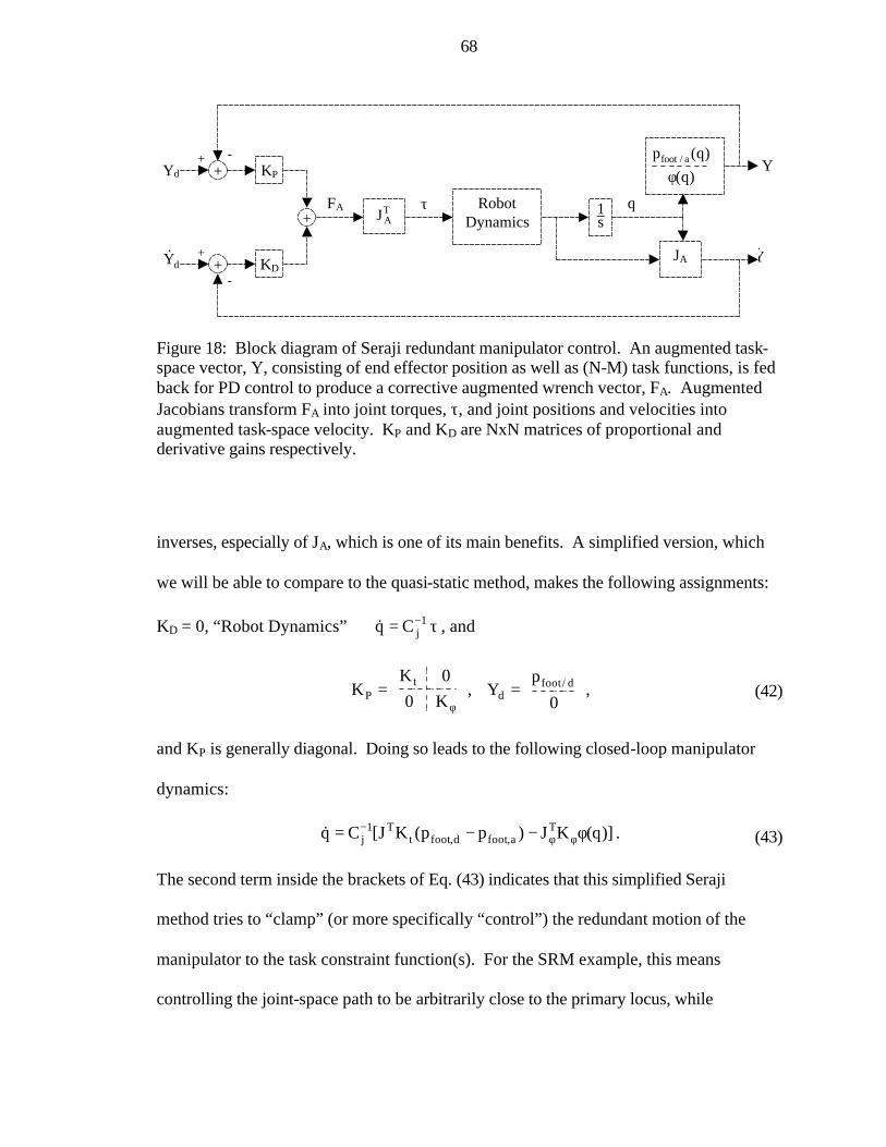
68

inverses, especially of JA, which is one of its main benefits. A simplified version, which

we will be able to compare to the quasi-static method, makes the following assignments:

KD = 0, “Robot Dynamics” ⇒ τ= −1jCq& , and

=

φK00K

K tP ,

=

0p

Y d/footd , (42)

and KP is generally diagonal. Doing so leads to the following closed-loop manipulator

dynamics:

)]q(KJ)pp(KJ[Cq Ta,footd,foott

T1j φ−−= φφ−& . (43)

The second term inside the brackets of Eq. (43) indicates that this simplified Seraji

method tries to “clamp” (or more specifically “control”) the redundant motion of the

manipulator to the task constraint function(s). For the SRM example, this means

controlling the joint-space path to be arbitrarily close to the primary locus, while

RobotDynamics

TAJ 1

s

KD

+

KP+

+

φ )q(

)q(p a/foot

JA

FA

+Yd Y

qτ

-

+

-

Y&dY&

Figure 18: Block diagram of Seraji redundant manipulator control. An augmented task-space vector, Y, consisting of end effector position as well as (N-M) task functions, is fed back for PD control to produce a corrective augmented wrench vector, FA. Augmented Jacobians transform FA into joint torques, τ, and joint positions and velocities into augmented task-space velocity. KP and KD are NxN matrices of proportional and derivative gains respectively.

69

simultaneously moving the end effector to the xd = -1 manifold. In this way, the quasi-

static and Seraji methods are somewhat complementary. But, like the quasi-static

method, the conditions that guarantee convergence to the primary manifold are unknown

(although increasing Kφ would seem to be a place to start).

At this point, it is reasonable to ask: Why employ simplified quasi-static

dynamics when this problem is, in its most direct form, purely kinematic? Both the

quasi-static and Seraji methods, which are energy methods, are inexact since they only

indirectly satisfy the goals of minimizing strain energy by appealing to physical intuition.

The reason is that both of these methods build on the standard “from the right” weighted

pseudoinverse of the Jacobian17,

J* = 1jC− JT (J 1

jC− JT)-1, (44)

where we could express a velocity form of Eq. (30) as

d/foot

* pJq && = . (45)

Eq. (44) is the well known minimum joint-space velocity pseudoinverse, such that using

it minimizes (dqT Cj dq) or ( qCq jT && ) for a given dpfoot/d or d/footp& . The use of 1

jC− as the

weight matrix is not accidental, since Eqs. (44) and (45) represent the dynamics that

result from the quasi-static model, Eq. (37), but with the joint-space springs removed and

only dampers acting. The critical problem with this pseudoinverse is its lack of

integrability [5] (although unfortunately, the SRM example cannot demonstrate this

because it only has one task-space DOF). Thus, in general, Eq. (23) is not realizable with

this method either.

17 Sometimes called the weighted Moore-Penrose pseudoinverse.

70

One obvious exact method would be to use the augmented Jacobian, JA, which, by

construction, is always square and invertible inside any possible region of interest. As

was derived for the SRM in Eqs. (34)-(36), this seems to be the most direct method. A

practical difficulty arises though, and that is that Eq. (31) (or (32)) can produce

intractably complex expressions for the task functions, φ(q)18. Further, as Eq. (34)

demonstrates, one needs to find several partial derivatives of these functions (a process

that resists an equivalent numerical implementation), and, in order to preserve

integrability, approximations to these derivatives would be fundamentally incorrect. It

would seem then that most real-world implementations of Seraji’s method would use

simpler task functions to keep complexity low. For instance, controlling the elbow

position of a redundant anthropomorphic manipulator is made easier by the fact that the

elbow position is only a function of a subset (a minority, maybe) of all the joint angles.

This is certainly not the case with Eq. (31) or (32).

Mussa-Ivaldi and Hogan [10] have specified the exact algorithm for simulating

movements directly along the primary locus (or any locus for that matter) using a

modified Moore-Penrose pseudoinverse (MMP) of the Jacobian. Their pseudoinverse

contains the proper correction factor so that, given a small displacement of the foot (end

effector) away from an equilibrium position, the corresponding joint-space displacement

results again in static equilibrium:

J* = (Kj – Γ)-1 JT (J (Kj – Γ)-1 JT)-1, (46)

where

18 Although simplifications can be made (which are not discussed in this thesis), the simplest two task

functions from Eq. (31) for a front leg of Robot 3, when expanded (using Mathematica’s ‘Expand’

71

Γ ⇒ Γi,l = ∑

= ∂∂∂M

1kk,foot

i

k,a/foot2

Fqq

p

l, (47)

or applied more directly to Robot 3 (M = 3, which are the three Cartesian components of

foot position),

Γi,l = z,foot

i

z,a/foot2

y,footi

y,a/foot2

x,footi

x,a/foot2

Fqq

pF

qq

pF

qq

p

∂∂∂

+∂∂

∂+

∂∂∂

lll. (48)

It is helpful to notice the similarity between Eqs. (46) and (44), and to then observe in

Figure 17 how the minimum joint-space velocity method always moves perpendicular to

the xd manifolds, while the exact methods move on a corrected path19. Mussa-Ivaldi and

Hogan refer to the NxN matrix, Γ, as a configuration dependent correction factor that

continuously modifies the new weight matrix, (Kj – Γ)-1. This modification method,

called the MMP pseudoinverse, produces an integrable differential form of Eq. (23). It

has a number of important features worth mentioning.

The MMP pseudoinverse, Eq. (46), is the Nullspace of Jφ, where φ(q) are derived

from Eq. (31) or (32). This makes the augmented Jacobian and the MMP complementary

methods.

The MMP method is much more practical than the augmented Jacobian for the

complex task of simulating minimum strain motion. Even working out Eq. (48), which

takes an additional partial derivative of the Jacobian, is very manageable.

function), contain 235 and 320 terms respectively.

19 The corrected path is the primary locus. For the SRM, this is that collection of points in joint-space where the line of JT passes directly through the unloaded equilibrium position. This applies to all other loci as well. Recall that JT is the local xd manifold normal vector, while is general terms, JT represents a hyperplane.

72

Γ is a function of the end effector force. The implementation details for the MMP

method, as described in [10], call for starting from the unloaded equilibrium position and

simultaneously updating the joint angles (q) and the end effector force (Ffoot) according to

qnew = qold + J* dpfoot/d, where J* is from Eq. (46), (49)

and

Ffoot,new = Ffoot,old + (J (Kj – Γ)-1 JT)-1 dpfoot/d. (50)

This, in my view, detracts slightly from the attractiveness of this approach, since it should

be possible to express the MMP pseudoinverse entirely from kinematics. This is in fact

the case, since, as noted previously, for any equilibrium position, Eq. (25) has a solution.

Therefore, we can replace Ffoot in Eq. (47) with

Ffoot = (J JT)-1 J Kj ∆q (51)

which makes the MMP pseudoinverse solely a function of q. It is important to remember

that Eqs. (46) - (51) are only applicable for points already satisfying Eqs. (31) and/or

(32), which is why we start at the unloaded equilibrium position. In fact, the MMP

pseudoinverse simply comes from a differential form of Eq. (25).

Regardless of which solution method is used, as long as it converges to the

primary locus the equilibrium configurations can be solved off-line and tabulated in a

look-up table. There are errors associated with interpolating between or extrapolating

away from tabulated values, especially if fine end effector control is needed. Fortunately,

few legged robots need fine foot position control. This argues for performing the

computationally intensive inverse kinematics solutions for Robot 3 off-line.

73

5.6 A Biological Perspective: Animal-Like Movements

As mentioned earlier, biological observations suggest that animals use the

minimum potential energy configurations to “solve” the redundancy problem. More

specifically, I would submit that animals move their limbs in the neighborhood of (but

not exactly on) a voluntarily changeable primary locus as demonstrated (abstractly) with

the SRM. Some researchers have proposed the “passive motion paradigm” [11], which

suggests that limb movement is achieved by simulating an externally imposed

displacement on the end effector (e.g. the task of swinging a leg or reaching for

something), with the redundant limb moving so that potential energy in the compliance of

the actuators is minimized. This is what any of the aforementioned solution methods

accomplish. The details of the configuration changes of the limb are parameterized by,

among other things, the individual compliance properties of the actuators.

It is reasonable to ask at this point: Why spend so much time and energy solving

for equilibrium solutions when an animal, with springy tendons and muscles, or a robot,

with spring-like actuators (i.e. braided pneumatic actuators [12]), will converge to an

inherent solution naturally? There could be multiple valid answers to this question, but I

will choose one that is important to Robot 3. First, the question assumes that something

(the environment, probably) applies a Ffoot that puts the foot at the desired task-space

location. There is no guarantee that this happens, especially during the swing phase of

the leg when, presumable, Ffoot = 0. Thus, the question does not address the very real

need to be able to place the foot of the redundant limb at a desired task-space location.

The control system must solve or learn something that allows it to do this – it doesn’t just

74

happen. If we, for the sake of argument, assume that τ represents a set of muscle or

actuator activations, and that the joint stiffnesses, Kj, are constant, then it is possible for

the control system to use the unique mapping

Ffoot = Ffoot(pfoot/d), (52)

in a region in which JA is nonsingular, to generate muscle activations according to

τ = JT Ffoot, (53)

which, acting on this spring-laden manipulator, will place the foot at pfoot/d. In this sense,

Ffoot doesn’t represent an actual force but a control system variable that maps a desired

foot position. Thus, to answer the previous question, the solution methods discussed

above, particularly Eqs. (46) - (48), (49), and (51) describe the procedure for finding an

Eq. (52) for any particular redundant animal-like limb (a limb that also satisfies the

singularity issues discussed above). The reason Eq. (23) is used instead of Eq. (52) is

that greater control flexibility is available for Robot 3 by having, on-hand, joint angle set-

points for a given pfoot/d. Once found, Eq. (23) leads trivially to activations for (constant

rate) spring-like actuators,

τ = Kj ∆q = Kj (q(pfoot/d) – qmr). (54)

This entire notion becomes very interesting and more animal-like when we allow the

joint-space stiffnesses to be changed with activation level, which is a topic for future

work.

75

5.7 Neural-Network Implementation

Using a neural-network at this juncture can be justified in four ways. First,

hidden-layer feed-forward neural-networks are reasonably good function estimators, and

provide convenient ways to embody, in a single operator, a look-up table. Second, it is

reasonable to assume that the tabular results of the simulations discussed above come

from a continuous smooth function (if the simulation converged to the primary locus) and

are therefore well behaved. Third, in the future, the inverse problem of relating the

structure of the trained neural-network (specifically connection weights) to the leg

kinematics may prove very useful. Finally, for this application, it is a small step to

reproduce a pseudoinverse Jacobian from the trained neural network.

With initial conditions set to q(0) = qmr, and knowing the leg kinematics, the

quasi-static simulation method is repeated off-line for a three-dimension Cartesian grid of

desired foot positions inside the workspace of the leg. Using back-propagation, a single-

hidden-layer feed-forward neural-network was trained to reproduce the mapping from

these desired Cartesian foot positions to optimal joint angles. Sigmoidal activation

functions were used for the hidden-layer neurons, with three of these neurons for each

joint-space DOF. Offsets for the hidden-layer neurons were included in the input weight

layer with a fourth, constant input equal to 1. Both input and output values of the neural-

network were scaled to be between ±1, with rescaled outputs being used as joint angle

set-points in the controller of Robot 3.

Mathematically, if the input and output scale factors are incorporated into their

respective weight layers, the output of the neural-network can be represented by

76

)net(sigWq O= , where

=

1p

Wnet d/footI , (55)

and sig(x) is assumed to operate on vectors element-by-element. Taking a time

derivative of equation (55), we get

d/footIO pW)net(DSIGWq && ′= , (56)

where

=

)net(dsig00

0)net(dsig0

00)net(dsig

)net(DSIG

HLN

2

1

L

MOMML

L

. (57)

Eq. (56) defines an approximate pseudoinverse of the Jacobian matrix,

IO

* W)net(DSIGWJ ′= . (58)

As one would expect, as “net” is a function of foot position, so also is the

pseudoinverse. By specifying desired foot positions as well as foot velocities, the trained

neural network can be used for both position and velocity control of the joints. The

precision of this approach, specifically the error between the desired foot trajectory and

that resulting from the output of the neural-network, will depend on the tolerances used in

training the neural-network. From an on-line computational cost perspective, given

adequate training (proportional to the accuracy needs of the robot), Eq. (58) represents a

significant computational savings over an exact pseudoinverse method, especially

considering it is solely a function of desired foot position.

77

5.8 Results and Conclusions

The coordinate system convention used with Robot 3 is as follows: +x = forward,

+y = left, +z = up. The reachable workspace of the left front leg foot of Robot 3 (in this

case, the foot is taken as the tibia-tarsis joint), from the shoulder or body-coxa joint, is a

complex shape contained inside a box of approximately: +8 in > x > -13 in, +13 in > y > -

7 in, +3 in > z > -12 in.

Inside this workspace, the quasi-static simulation solution method discussed

above, with joint limit detection (Eq. (40)), was used to find stable equilibrium solutions

x

y

Figure 19: Partial overhead view of Robot 3 showing left front leg x-y coordinate system used for inverse kinematics studies. The origin is the body-coxa joint, which is where the leg attaches to the body. This view looks in the –z direction.

78

for 152 desired foot positions in a Cartesian grid with a 2 inch spacing (2x2x2 inch

cubes). The simulations were completed with typical final errors between actual and

desired foot positions of less than 1/100 of an inch, although some foot positions on the

fringes of the workspace resulted in greater errors. In all cases, the network was trained

to the final achieved foot position, not desired. After neural-network training, typical

foot position error (between desired, or network input, and achieved, or that resulting

from network output) was less than 1/20 of an inch. No efforts were taken to rigorously

characterize the performance of the neural-network, as it was deemed sufficient for Robot

3.

In order to check whether the equilibrium solutions found using the quasi-static

method were on the primary locus, the MMP method, without joint limit detection, was

used to simulate the same movements. The results indicated that the quasi-static method

did indeed converge to the primary locus for all solutions inside the reachable joint-space.

The only differences occurred when the primary locus solution called for a joint-space

location outside the reachable region. In these cases, the quasi-static method slides along

the joint limit boundary until a minimum energy solution is found, while the MMP

method ignored the boundaries. In the future, I would like to examine the correct ways to

modify the exact method to account for joint limits during simulated movement. One

obvious shortcut would be to increase the appropriate joint stiffness exponentially at the

corresponding joint-space boundary, although, in my experience, this can lead to some

numerical problems. Ultimately, the issues of singularities and solution uniqueness need

to be reexamined along joint-space boundaries.

79

Figure 20 and Figure 21 show test runs of the neural network for two given foot

trajectories in the x-y plane (pfoot/d,z = -6 inches below the shoulder). In Figure 20, the

desired foot position traces a 5 inch radius circle (shown), while in Figure 21, the foot

traces a 7 x 7 inch square (shown). In the case of the circle, the maximum ±z error was

+0.51 / -0.25 inches, and for the square, maximum ±z error was +0.26 / -0.17 inches.

80

- 10 - 5 0 5 10

- 5

0

5

10

15

Figure 20: Desired circular foot path vs. neural-network output. The trained neural-network outputs joint angles for desired foot positions along a 5 inch radius circular path in the x-y plane, with pfoot/d,z = -6 inches below the body-coxa joint. These joint angles result in a slightly distorted actual foot position path.

- 10 - 5 0 5 10

- 5

0

5

10

15

Figure 21: Desired square foot path vs. neural-network output. The trained neural-network outputs joint angles for desired foot positions along a 7x7 inch square path in the x-y plane, with pfoot/d,z = -6 inches below the body-coxa joint. These joint angles result in a slightly distorted actual foot position path.

x

y

x

y

81

As an example case, for the arbitrary desired foot position of pfoot/d = {-1,9,-5}

inches, the actual foot position of pfoot/a = {-0.89, 9.09, -5.13} inches is achieved.

Calculating an approximate pseudoinverse using Eq. (58) for the same arbitrary desired

foot position, and premultiplying by the actual Jacobian for the leg configuration

resulting from Eq. (55), produces

−−−

−=

92.004.002.002.001.103.0

26.016.007.1JJ * . (59)

If the pseudoinverse was exact, the above would be the identity matrix. Thus, for the

arbitrary desired foot velocity of d/footp& ={1,1,1} in/s, the actual foot velocity of a/footp&

={1.16, 0.97, 0.91} in/s is achieved. These results are typical throughout the workspace

with errors increasing slightly at the fringes. In the future, the target points for the quasi-

static simulation should be taken from a region artificially enlarged over the normal

workspace, thus deliberately reaching for points outside the workspace. Training the

neural-network on this “oversized” mapping may be more difficult, but should also help

to decrease the over-sensitivity, or position errors, of the network to desired foot

positions at the edges of the workspace.

A natural question is to ask how the approximate pseudoinverse derived above

compares with the exact pseudoinverse, Eq. (46). The results were crudely approximate

for several arbitrary test points throughout the workspace. This was expected because of

the approximate nature of this simple neural-network scheme. Practically, I find the

trade-offs between this approximate method (online computational speed) and an exact

method (kinematic precision) to be quite worthwhile. Of course once joint-space

82

boundary issues are resolved, tabular results could be obtained through the exact method

and mated with a neural-network to achieve the same.

A second natural question is to compare the joint-space trajectories of this method

with actual kinematics from a Blaberus cockroach. A partial investigation and

comparison was performed [13] and the results were remarkable (see Figure 22). Forceps

were used to move the tibia-tarsis joint of a deinnervated left front cockroach leg through

a walking cycle motion. The motion was filmed and digitized to produce joint-space

trajectories and scaled foot motions. Even using independent, linear joint-space

compliance functions, trajectories for the four proximal joints compared well. The

femur-tibia joint trajectory did not compare well though, and it is most likely the case that

these joint-space compliance functions are too simplistic, or (more likely), the forceps

applied an unknown environmental moment to the tibia.

The scheme described in this chapter is being used for the locomotion controller

for Robot 3. With the robot suspended by tethers, and the neural-networks supplying

joint-space set-points for local position control loops, Cruse-based leg coordination

mechanisms [14] (also see Appendix) cause the robot to swim in a smooth tripod gait

(see Figure 23).

Works Cited 1 Homayoun Seraji. Configuration Control of Redundant Manipulators: Theory and

Implementation. IEEE Transactions on Robotics and Automation, Vol. 5, No. 4, August, 1989.

2 D. E. Whitney. Resolved motion rate control of manipulators and human prostheses. IEEE Trans. Man-Machine Syst., MMS-10(2):47-53, 1969.

83

3 A. Liegeois. Automatic supervisory control of the configuration and behavior of

multibody mechanisms. IEEE Trans. Sys. Man Cybernet., SMC-7(12):868-871, 1977.

4 J. M. Hollerbach and K. C. Suh. Redundancy resolution of manipulators through torque optimization. In Proc.1985 IEEE Int. Conf. on Robotics and Automation (ICRA’85), St. Louis, pp. 1016-1021, 1985.

5 C.A. Klein and C.H. Huang. Review of pseudoinverse control for use with kinematically redundant robot manipulators. IEEE Trans. System., Man, Cybern., vol. SMC-13, no. 3, pp. 245-250, 1983.

6 G.M. Nelson and R.D. Quinn. A numerical solution to inverse kinematics for swing control of a cockroach-like robot. 4th International Conference on Climbing and Walking Robots (CLAWAR’01), eds. K. Berns, R. Dillmann, Karlsruhe, Germany, pp. 347-354, September, 2001.

7 J. T. Watson and R. E. Ritzmann. Leg kinematics and muscle activity during treadmill running in the cockroach, Blaberus discoidalis: I. Slow running. J. Comp. Physiol., A182: 11-22, 1998.

8 G.M. Nelson. Modeling and Simulation of an Insect-like Hexapod. Master’s Thesis, Case Western Reserve University, Cleveland, OH, August, 1995.

9 L. Sciavicco and B. Siciliano. A dynamic solution to the inverse kinematic problem for redundant manipulators. In Proceedings of the 1987 IEEE International Conference on Robotics and Automation, Raleigh, NC, pp. 1081-1087, April, 1987.

10 F.A. Mussa-Ivaldi, N. Hogan. Integrable Solutions of Kinematic Redundancy via Impedance Control. Int. J. of Robotics Research, Vol. 10, No. 5, pp. 481-491, October, 1991.

11 F. A. Mussa-Ivaldi, P. Morasso, R. Zaccaria. Patterns of interarticulator phasing and their relation to linguistic structure. Biological Cybernetics, Vol. 60, pp. 1-16, 1988.

12 R.W. Colbrunn, G.M. Nelson, and R.D. Quinn. Modeling of Braided Pneumatic Actuators for Robotic Control. Proceedings of the 2001 Int. Conf. on Intelligent Robots and Systems (IROS), Maui, HI, 2001.

13 G. M. Nelson, R.D. Quinn, J. T. Watson, R. E. Ritzmann. A numerical solution to inverse kinematics for the control of robotic leg movement. Soc. Neurosci. Abstr., Online: http://www.sfn.org/, 2000.

14 H. Cruse. What mechanisms coordinate leg movement in walking arthropods? Trends in Neural Science, Vol. 13, pp. 15-21, 1990.

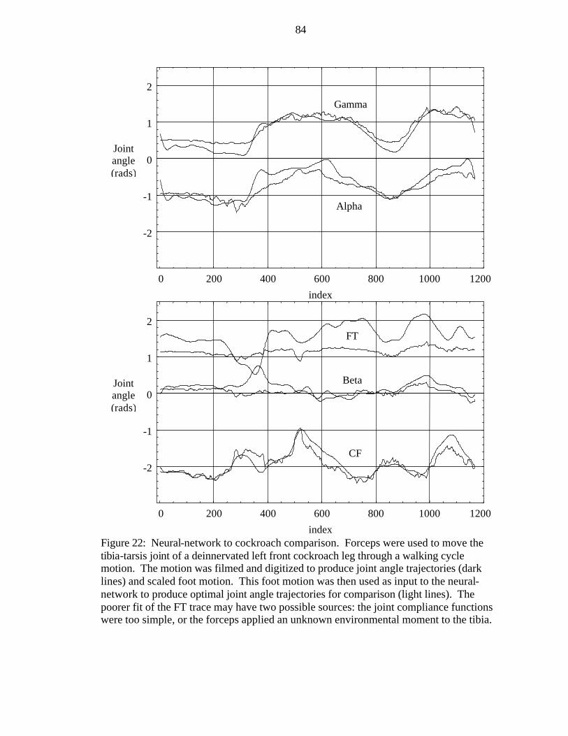
84

2

1

0

-1

-2

120010008006004002000

Jointangle(rads)

Gamma

Alpha

index

2

1

0

-1

-2

120010008006004002000

Jointangle(rads)

index

FT

CF

Beta

Figure 22: Neural-network to cockroach comparison. Forceps were used to move the tibia-tarsis joint of a deinnervated left front cockroach leg through a walking cycle motion. The motion was filmed and digitized to produce joint angle trajectories (dark lines) and scaled foot motion. This foot motion was then used as input to the neural-network to produce optimal joint angle trajectories for comparison (light lines). The poorer fit of the FT trace may have two possible sources: the joint compliance functions were too simple, or the forceps applied an unknown environmental moment to the tibia.

85

Figure 23: Snapshots of Robot 3 air-walking in a tripod gait. The sequence of snapshots, cropped from digital video of the robot, goes from left to right, top to bottom. In the first snapshot, the near-side middle leg is in stance while the front and rear legs transition to swing. In the second snapshot, the front and rear legs are in full swing. In the third snapshot, they transition into stance, while in the fourth snapshot, the middle leg transitions to swing.

86

Chapter 6

Local Control Implementation Details

In this chapter, I will discuss some of the details of local control implementation

for Robot 3. I will begin by describing the current control system setup, including

improvements and implications in the way the higher and lower level controllers work

together. An overview of two different detailed revisions of the low level controller will

then be given. The chapter will conclude with a discussion of and comparison between

several different PWM implementations as well as a feasible PFM implementation.

6.1 Improvements in the Robot 3 control system

As Figure 11 shows, the posture controller for Robot 3 was originally

implemented in a triangular control system setup. And as the results of just posture

control indicated, it was clear that a more hierarchical system was needed – one that had

distinct high and low level controllers that could each perform separate yet overlapping

tasks at different speeds. I envisioned that the lower level control (LLC) would be closest

to the physical robot and would perform stereotyped but adjustable tasks as rapidly as

possible. This would include spring-like position control of individual joints. In order to

realize this, the LLC would be responsible for reading the sensors of the robot, making

this afferent data available to the high level controller (HLC), and rapidly adjusting duty

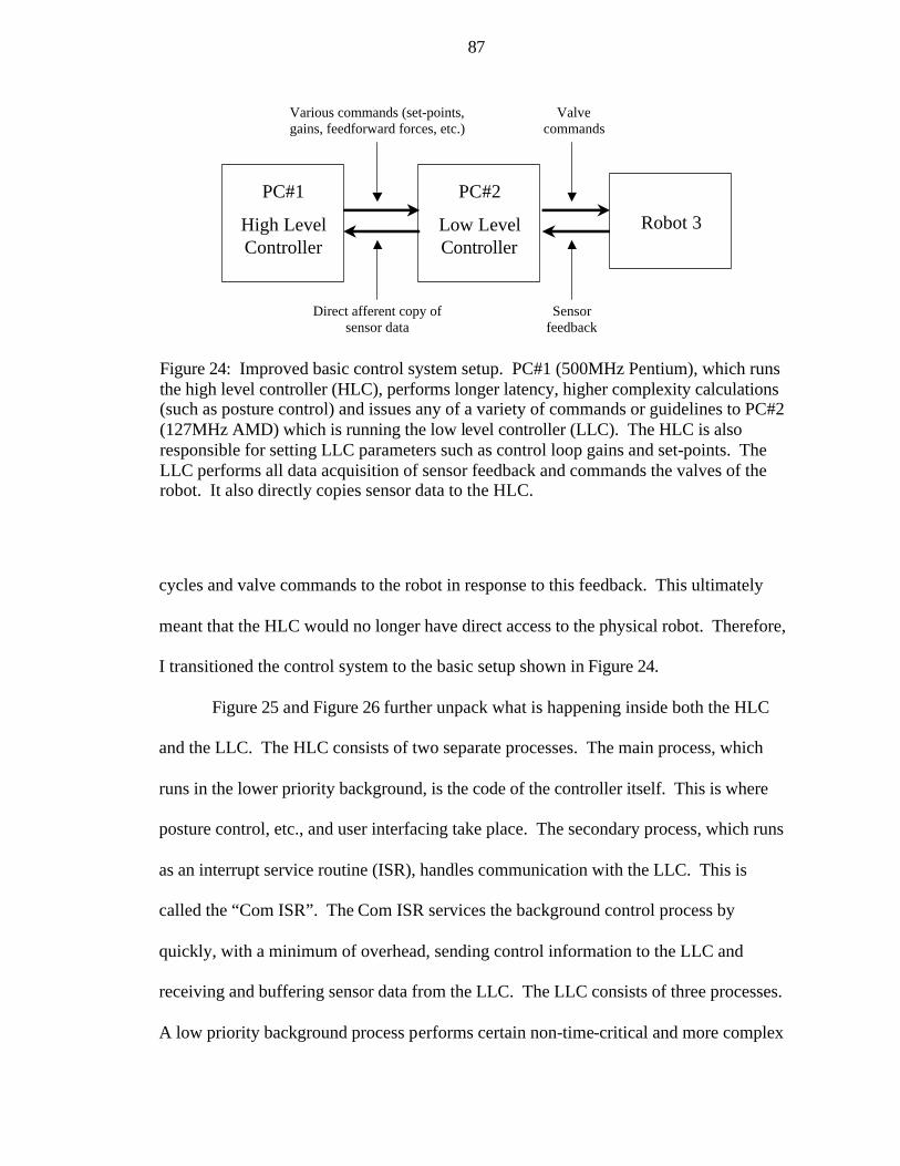
87

cycles and valve commands to the robot in response to this feedback. This ultimately

meant that the HLC would no longer have direct access to the physical robot. Therefore,

I transitioned the control system to the basic setup shown in Figure 24.

Figure 25 and Figure 26 further unpack what is happening inside both the HLC

and the LLC. The HLC consists of two separate processes. The main process, which

runs in the lower priority background, is the code of the controller itself. This is where

posture control, etc., and user interfacing take place. The secondary process, which runs

as an interrupt service routine (ISR), handles communication with the LLC. This is

called the “Com ISR”. The Com ISR services the background control process by

quickly, with a minimum of overhead, sending control information to the LLC and

receiving and buffering sensor data from the LLC. The LLC consists of three processes.

A low priority background process performs certain non-time-critical and more complex

PC#1

High LevelController

PC#2

Low LevelController

Robot 3

Various commands (set-points,gains, feedforward forces, etc.)

Direct afferent copy ofsensor data

Valvecommands

Sensorfeedback

Figure 24: Improved basic control system setup. PC#1 (500MHz Pentium), which runs the high level controller (HLC), performs longer latency, higher complexity calculations (such as posture control) and issues any of a variety of commands or guidelines to PC#2 (127MHz AMD) which is running the low level controller (LLC). The HLC is also responsible for setting LLC parameters such as control loop gains and set-points. The LLC performs all data acquisition of sensor feedback and commands the valves of the robot. It also directly copies sensor data to the HLC.

88

calculations, such as calculating the Jacobian of each leg. A middle priority process, the

communications ISR (Com ISR), is responsible for communication with the HLC. The

highest priority process is the PWM ISR, which is the core of the LLC. The PWM ISR

reads sensors, performs control calculations, and commands valves.

The communications structure depicted in Figure 25 suffered from a priority

bottleneck which adversely affected the speed with which the HLC could talk with the

PWM ISR. The flow of data to and from the PWM ISR is handled by the background,

which is the lowest priority process of the LLC. Figure 26 shows how the

communications system was changed to avoid this problem. The Com ISR was rewritten

PWM ISR

Com ISRTx

Mem

Rx

Background

Rx

Background Mem

Com ISRRx

Tx

Low Level Control High Level Control

Tx

RxTx

Robot 3

16 byteFIFOs

16 byteFIFOs

115200 bps

Ring buffers Ring buffers

Figure 25: Control system communications structure. The HLC consists of two processes: a lower priority background process running the actual HLC code and a higher priority communications ISR (Com ISR). The LLC consists of three processes: a lower priority background process that performs certain non-time-critical calculations as well as moving data to and from the Com ISR buffers and memory, a middle priority process (the Com ISR), and a high level PWM ISR which does elementary control calculations, A/D conversions and valve commanding. One problem with this setup is that the flow of data to and from the PWM ISR to the HLC is handled by the low priority background process.

89

such that it could receive structured data streams, assemble the individual pieces of data,

and directly copy these into system memory. For instance, the PWM ISR not only stores

sensor data for use in the LLC, it also copies this data directly to the 16 byte transmit

FIFO of the UART serial communication link. The HLC Com ISR assembles this data as

it is received and copies completed data valves into memory to be used by the HLC. The

same method is used in the opposite direction, except that flow control is implemented so

that the rather busy LLC is not overwhelmed with data. With this setup, a full posture

control update is possible every PWM period at 80 Hz (which is 12.5 ms).

PWM ISR

Mem Background Background Mem

Low Level Control High Level Control

Flow Control

Robot 3

16 byteFIFOs

16 byteFIFOs

115200 bps

Buffers Buffers

Com ISRTx

Rx RxCom ISR

Rx

TxTx

RxTx

Figure 26: Improved control system communications structure. This is an improvement on the structure in Figure 25. Now the LLC PWM ISR not only stores sensor data in memory but it also directly copies this same data to the serial communications transmit (Tx) FIFO buffer for immediate dispatch to the HLC. Also, both the HLC and LLC Com ISRs directly access memory through structured buffers. As a result, the LLC background process is no longer involved in data flow. Flow control is implemented from the HLC to the LLC so that the HLC can dump arbitrarily large chunks of data into the Com ISR transmit buffer.

90

The PWM ISR also operates such that the low level controller updates duty cycles

at the PWM frequency. In other words, at the beginning of every PWM period for each

valve, the LLC has calculated a new duty cycle based on new sensor feedback taken at

that time. Because the pneumatic valves can only operate in the 50-100 Hz range, time

division multiplexing makes this optimized update scheme possible. Figure 27 depicts

and explains this process.

91

1 sec

80 PWM periods at 80 Hz

12.5 ms =1/80 sec

100 PWM interrupts at 8 kHz

125 µs =1/8000 sec 125 µs 125 µs 125 µs

initiate12 bit

conversion

initiate12 bit

conversionread channel #1perform control calcsset A/D to channel #2

read channel #2perform control calcsset A/D to channel #3

PWM period beginsfor all valves relying

on LLC feedbackfrom channel #1 only

The ON/OFF valve commandsare issued at the beginning ofeach PWM interrupt so that thetiming is precise. Thus, there isa single PWM interrupt delaybetween the beginning of thePWM period and the actualvalve commands.

valve command ON

valve command ON

initiate12 bit

conversion

PWM period beginsfor all valves relying

on LLC feedbackfrom channel #2 only

Figure 27: Time division multiplexing as applied to Robot 3. At 80 Hz PWM, there are 80 PWM periods in one second. Each PWM period is divided into 125 µs intervals by 100 PWM interrupts, which occur at 8 kHz. The PWM ISR alternates between different tasks on each interrupt. When all the sensors needed for calculating the control law for a group of valves are read (i.e. the duty cycles for the valves that run a joint), the PWM period for those valves begins. There is a one PWM interrupt delay from the beginning (end) of the PWM period and the ON(OFF) valve commands. This is because the valve commands are issued at the beginning of that PWM interrupt in order that the interval timing of the duty cycle be precise. When the PWM period completes, the entire process is repeated.

92

Figure 28, which corresponds to Figure 25, shows a detailed system diagram of

how the LLC and robot interfaced before the communications improvements were made.

Here is a brief overview of this system. The bottom box, labeled “Robot 3”, consists of

the electronics and physical robot. The electronics are essentially the same as those

depicted in Figure 12 except for the inclusion of low pass filters (“L.P.F”) on the strain

gage signals20. The LLC interfaces with the robot through the 12 bit A/D card and a 48

channel digital I/O card (“D I/O”). The three processes of the LLC communicate through

memory, which is conceptually divided into “high”, “background”, and “PWM ISR”

levels. Inside the PWM ISR, the counter “global_cycle_time” is used to schedule the

various interrupt actions in time. The variable “chan” represents which A/D channel is

being accessed during the ISR execution. As indicated previously, when triggered, the

first thing the PWM ISR does is issue valve commands. These commands were updated

during the previous interrupt according to the current duty cycles produced by the control

system.

20 These strain gages are the three half-bridge load cells that measure foot force. They are not the gages

indicated in Figure 12, which were removed from the robot.

93

Physical Robot

OptosL.P.F.

PowerSupply

#2

PowerSupply

#1

L. Bank U. Bank

A/D D I/O

+12 V

Valvedrivingsignal+12 V

COM

Gage sigground

FilteredGage sig

±5 V

Gage sigground

Gage sig±5 V

+12 V

+5 V

-12 V

COM

Valvecommands

Pot sig0-5 V

100 psig air

AMDAm5x86127 MHz

Shared memory

short port#deltashort port#command

long unsigned int realtimeshort global_cycle_time

int potreading[24]

short force_mode_on

int educyc[24]

float stiffness[24]unsigned int setpoint[24]

int fducyc[24]

int fffcom[24]int effcom[24]

short pot_chan_to_leg_map[24]

float gf[6]

float posloadforce[6]

float ptrfx[6]float ptrfy[6]float ptrfz[6]

float posloaddir[6][3]

float fbartrans[24]

short complete_flex_inhibshort complete_ext_inhib

float jact[24][3]

float aratio[24]

valve_curve vcurve[24].edc[94]valve_curve vcurve[24].fdc[94]

short epstate[24]short fpstate[24]

short joint_enabled[24]

int gagereading[18]

float ftrans[6][3]

float newjact[24][3]float newftrans[6][3]

float newposloaddir[6][3]

short cycle_time[24]

short closetiming[101]short opentiming[101]

short ebit[24]short fbit[24]

high level

background level

PWM I.S.R. level

short adchannum[42]

Issue valve commands (turn valves on/off)Update counters

PICU

global_cycle_time Actions

0,2,4,6…82Waypoint calculations.Initiate 12 bit conversion.

1,3,5,7…47

Local joint + leg + posture control calc. Determine duty cycles.Calculate foot force at leg from posture command and load feedbackLocal joint position control w/coactivation calculation.Reset cycle_time = 0.Set A/D multiplexer to next channel.Change A/D voltage range to ± 5V.Read pot channel.

49,51,53…83

Enforce deadband on +load feedback force.Calculate +load feedback force.Set A/D multiplexer to next channel.Change A/D voltage range to 0 to +5V.Read gage channel.

(chan)

(0,1,2,3…41)

(0,1,2,3…23)

(0,5,10,14,18,21)

float totalfx, totalfy, totalfz(23)

(41)(24,25,26…41)

84 - 89 Waypoint calculations.90 - 95 If available, update jact, posloaddir, ftrans from background calcs.96 - 99

(0,1,2,3…23)

Low level controlUpdate valve commands and valve states

(0,1,2,3…23)(0,1,2,3…23)(0,1,2,3…23)

(0,1,2,3…23)

(24,25,26…41)(24,25,26…41)

PWM I.S.R.

UART

Communications I.S.R.16 byte RX FIFO16 byte TX FIFO

RECEIVE RING-BUFFERSEND RING-BUFFER

comlink::getbyte/int/shortfloat/floatcomlink::putbyte/int/shortfloat/float

command message? command programsrecv###, enable/disable

send###

YES

NO

kinematicmodeling

oflegs

communications layer

8 kHzinterrupt

Highestpriority

Middlepriority

Background

Lowestpriority

to HLC

PWM ISRexecution

order

LLCrunning on

PC#2

Robot 3

Figure 28: Low level controller details corresponding to Figure 25. See text for details.

94

The background process is continuously calculating several essential kinematic

transformations, such as Jacobians and joint linkage transmission factors. Even though

this is a background process on the LLC, this is considerably faster than having the HLC

calculate these quantities for the LLC (which would involve shipping the necessary

sensor data to the HLC, and shipping the kinematic values back). Before the

communication fix discussed in Figure 26, the LLC was itself controlled by “command

message(s)” issued by the HLC. Those command messages corresponded to “command

programs”, each of which performed “send”, “recv(receive)”, or “enable/disable” actions.

For instance, in order for the HLC to get sensor data, it would send a command message

to the LLC, which would cause the background process to send the requested data to the

Communications ISR, where it was dispatched to the HLC. This system, though

suffering from the aforementioned problem, worked well in terms of avoiding memory

usage conflicts and communications flow control issues. In fact, the air-walking local

control results discussed in Chapter 5 used this setup.

Figure 29 corresponds to Figure 26. Here, the LLC communications bottleneck

has been removed by having the PWM ISR send sensor data directly to the serial

communications link (“UART”). Also, the Com ISR assembles incoming data in a

“structured rec(eive) buffer” and then copies this data into the appropriate “high level”

memory location.

95

Physical Robot

OptosL.P.F.

PowerSupply

#2

PowerSupply

#1

L. Bank U. Bank

A/D D I/O

+12 V

Valvedrivingsignal+12 V

COM

Gage sigground

FilteredGage sig

±5 V

Gage sigground

Gage sig±5 V

+12 V

+5 V

-12 V

COM

Valvecommands

Pot sig0-5 V

100 psig air

AMDAm5x86127 MHz

Shared memory

short port#deltashort port#command

long unsigned int realtimeshort global_cycle_time

int potreading[24]

short force_mode_on

int educyc[24]

float stiffness[24]unsigned int setpoint[24]

int fducyc[24]

int fffcom[24]int effcom[24]

short pot_chan_to_leg_map[24]

float gf[6]

float posloadforce[6]

float ptrfx[6]float ptrfy[6]float ptrfz[6]

float posloaddir[6][3]

float fbartrans[24]

short complete_flex_inhibshort complete_ext_inhib

float jact[24][3]

float aratio[24]

valve_curve vcurve[24].edc[94]valve_curve vcurve[24].fdc[94]

short epstate[24]short fpstate[24]

short joint_enabled[24]

int gagereading[18]

float ftrans[6][3]

float newjact[24][3]float newftrans[6][3]

float newposloaddir[6][3]

short cycle_time[24]

short closetiming[101]short opentiming[101]

short ebit[24]short fbit[24]

high level

background level

PWM I.S.R. level

short adchannum[42]

Issue valve commands (turn valves on/off)Update counters

PICU

global_cycle_time Actions

0,2,4,6…82Waypoint calculations.Initiate 12 bit conversion.

1,3,5,7…47

Local joint + leg + posture control calc. Determine duty cycles.Calculate foot force at leg from posture command and load feedbackLocal joint position control w/coactivation calculation.Reset cycle_time = 0.Set A/D multiplexer to next channel.Change A/D voltage range to ± 5V.Read pot channel.

49,51,53…83

Enforce deadband on +load feedback force.Calculate +load feedback force.Set A/D multiplexer to next channel.Change A/D voltage range to 0 to +5V.Read gage channel.

(chan)

(0,1,2,3…41)

(0,1,2,3…23)

(0,5,10,14,18,21)

float totalfx, totalfy, totalfz(23)

(41)(24,25,26…41)

84 - 89 Waypoint calculations.90 - 95 If available, update jact, posloaddir, ftrans from background calcs.96 - 99

(0,1,2,3…23)

Low level controlUpdate valve commands and valve states

(0,1,2,3…23)(0,1,2,3…23)(0,1,2,3…23)

(0,1,2,3…23)

(24,25,26…41)(24,25,26…41)

PWM I.S.R.

UART

Communications I.S.R.16 byte RX FIFO16 byte TX FIFO

STRUCTURED REC BUFFER

command message? YES

NO

kinematicmodeling

oflegs

communications layer

8 kHzinterrupt

Highestpriority

Middlepriority

Background

STOPLowestpriority

to HLC

PWM ISRexecution

order

LLCrunning on

PC#2

Robot 3

sensordata

Figure 29: Low level controller details corresponding to Figure 26. See text for details.

96

Finally, it is only fair to note that the 115200 bps serial link may be considered a

communications bottleneck itself. It turns out to not be a serious limitation. The serial

link can send one byte of data in just under 87 µs. Thus, pure communications time for

sending the entire sensor data set (84 bytes), plus time (4 bytes), to the HLC is

approximately 7.7 ms. Because the Com ISR also implements a short-float data type (a

16 bit float), it is possible to send six posture control foot forces back to the LLC in

approximately 3.1 ms. Thus the total communications time is approximately 10.8 ms,

which is less than a single PWM period. As mentioned previously, for future projects I

have actively endorsed a transition to real-time Linux because it should be possible to run

both the HLC and LLC on a single powerful desktop computer.

6.2 Pulse actuation implementation issues

After being energized from a fully deenergized state, the solenoid valves used on

Robot 3 (Matrix 750 series, three-way, 8 channel, made by Matrix S.p.A of Italy), when

pressurized at 100 psig, take about 4 ms to open. The valves take about 1 ms to close

after being deenergized from a fully energized state. The implications of this are that the

actual duty cycle, that being the period of time when the physical valve is open, is

different from the commanded duty cycle, which is the electrical driving signal sent to

the valve. If we assume that the opening and closing events are instantaneous, then at 50

and 80 Hz PWM, the relationships shown in Figure 30 exist between commanded and

actual duty cycles. For this idealized valve, commanded duty cycles less than the open

97

response time never open the valve. Once the valve is open, it is not possible to produce

duty cycles less than the close time. The opposite effect happens for large duty cycles

approaching 100%.

One aspect of this behavior that could be important to Robot 3 and future robots is

the noticeable shrinkage of the linear sloped region in Figure 30 as PWM frequency

increases. This is expected since as the PWM period decreases, the valve delays become

a larger percentage of this duration. As a result, it appears from my experience that the

variability from valve to valve increases with PWM frequency, which is generally

unhelpful for resolving control issues. In this sense, in the future it may actually be better

0 10 20 30 40 50 60 70 80 90 100

0

10

20

30

40

50

60

70

80

90

100

ActualDuty Cycle

CommandedDuty Cycle

50 Hz

80 Hz

Figure 30: Relationship between commanded and actual duty cycles due to valve delay properties. The valves are Matrix 750 series (8 channel) three-way solenoid valves. When pressurized to 100 psig, the open delay is approximately 4 ms, while the close delay is slightly under 1 ms.

98

to use lower PWM frequencies, and use some the issues discussed below in this section to

recover the lost bandwidth.

The open delay value was verified by measuring, with an oscilloscope, the voltage

drop across a low resistance electrically in series with the valve. An inductive transient,

or “kick”, could be observed when the shutter of the valve opened (see [1] for more

details). Of course, this little trick meant that I could observe the electromechanical

behavior of the valve in the discontinuous regions of Figure 30. Figure 31 shows the

results of this investigation for 80 Hz PWM.

The best way to interpret Figure 31 is to choose a commanded duty cycle along

the x axis, and to then follow events up the plot with time. Consider a 50 % commanded

duty cycle. At time = 0, the valve starts from a cold start and is energized. At

normalized time = 0.32, which is 4 ms into an 80 Hz PWM period, the valve opens. At

normalized time = 0.5, the valve is deenergized, and at normalized time = 0.58 the valve

closes. (The close time is 1 ms after the deenergizing time, which is 0.08 in normalized

time for 80 Hz PWM.) This process is repeated for the next PWM period. As this plot

indicates, things change for commanded duty cycles above 92 %. Since the actual close

time now comes after the new commanded open time, there is some energy still stored in

the valve. As a consequence, the valve takes less time to open. The higher the

commanded duty cycle above 92 %, the lower the open delay of the valve until, at 98 %,

the valve stays open continuously. This result seems to verify the 1 ms close time for the

valves, since this effect begins around 92 %, leaving 1 ms of 80 Hz PWM period

available before the next energize command.

99

0 50 10010 20 30 40 60 70 80 90

1.0

0

0.9

0.7

0.8

0.5

0.6

0.3

0.4

0.2

0.1

1.1

1.2

1.3

1.4

1.5

1.6

1.7

1.8

1.9

2.0

energize(cold start)

energize

energize

deenergize

deenergize

valve opens

valve opens

valve closes

valve closes

Commanded Duty Cycle

Normalized time =

time PWM period (= 12.5ms)

Figure 31: The effects of valve delays on actual open and close times at 80 Hz PWM. The bold horizontal lines represent when the valve is energized, while the bold sloped lines represent when the valve is deenergized. The respective light lines represent when the valve opens or closes. Given a commanded duty cycle, the valve takes 32% (4ms) of the PWM period to open from a cold start, and 8% (1ms) to close after being deenergized. For commanded duty cycles above 92%, this close delay advances the open time substantially.

100

0 50 10010 20 30 40 60 70 80 90

1.0

0

0.9

0.7

0.8

0.5

0.6

0.3

0.4

0.2

0.1

1.1

1.2

1.3

1.4

1.5

1.6

1.7

1.8

1.9

2.0

energize

energize

deenergize

deenergize

valve opens

valve opens

valve closes

valve closes

Commanded Duty Cycle

energize(cold start)

Normalized time =

time PWM period (= 12.5ms)

Figure 32: Warping valve command times to normalize actual valve open time. By sliding normalized time for commanded duty cycles above 92%, it is possible to cause the valve to open at the same time each PWM period.

101

This behavior suggests a way in which the 4 ms delay of the valve can be

effectively canceled. Consider Figure 32. The interpretation of this figure follows from

Figure 31. Consider commanded duty cycles above 92 %. By “sliding”, or warping, the

time axes for duty cycles in this region, it is possible to cause the valve to open at the

same time during each PWM period. This “sliding” simply means delaying the

commanded deenergize and energize times. The actual valve open time now becomes

the beginning of the PWM period, and we now think in terms of actual valve open time

0 10 20 30 40 50 60 70 80 90 100

0

0.1

0.2

0.3

0.4

0.5

0.6

0.7

0.8

0.9

1

deenergize

energize

Normalized time =

time PWM period (= 12.5ms)

Commanded Duty Cycle

valve opens

valve opens

New PWMperiod

Figure 33: Valve pretensioning timing curves for 80 Hz predicted PWM. The “New PWM period” is now bounded by when the valve actually opens, not the valve commands. The once-per-PWM-period control loop update is now performed when the valve opens. If the control law calls for duty cycles below the valve open delay (32% at 80 Hz PWM), the valve is deenergized immediately and the active force output of the actuator is negligible.

102

and not commanded valve open time. Figure 33 shows the scheme as it is currently used

on Robot 3. By performing the once-per-PWM-period control loop update (basically a

sensor read) at the actual open time, instead of the commanded open time, some control

bandwidth can be recovered, albeit a small amount (and every bit counts!). I call this

“valve pretensioning” using “predicted PWM” because the scheme energizes the valve

before the beginning of the PWM period in anticipation of the actual open time. For

commanded duty cycles below the open delay time (32% for 80 Hz PWM), the valve is

still energized for this percentage of the PWM period but the active force output of the

actuator is negligible.

Matlab/Simulink models have been used to verify this bandwidth improvement.

In fact, Simulink has been used to compare several different pulse actuation schemes,

including three different implementations of PWM, as well as pulse-frequency-

modulation (PFM). Figure 34 shows each pulse actuation scheme and how they respond

to a given changing input signal. I’ve called the schemes simple PWM, continuous

PWM, predicted PWM, and PFM.

103

15 Hzinput signal

50 HzPWM counter

simple50 Hz PWM

continuous50 Hz PWM

predicted50 Hz PWM

10 ms pulsePFM

0 20 40 60 80 100

Commandedduty cycle (%)

or pulsefrequency (Hz)

50

0

100

valve open

valve energized

valvedeenergized/

closed

time (ms)

Figure 34: Four different pulse actuation schemes. These results are examples taken from the simulation depicted in Figure 35. The input signal is a 15 Hz sinusoid that was chosen to exaggerate the differences between the different schemes. Also, a 50 Hz PWM counter signal (saw-tooth) is shown with the input signal for reference.

104

The plots in this figure are taken from Simulink models such as that shown in

Figure 35. The pulse actuation scheme box (in this case “simple PWM”) takes as input

commanded duty cycle (“CDC”), a PWM frequency (“PWM freq”), and outputs a

commanded pulse train (“CPT”) which is a binary signal of valve commands (ON/OFF

or energize/deenergize) versus time. This CPT is then fed into an “Electromechanical

Valve Model” which empirically models the valve delay properties discussed previously.

The output of this box is an actual pulse train (“APT”) which is a binary signal of actual

valve open/close states versus time. This model includes both the open and close delay

behaviors, and it also approximates the high duty cycle behavior discussed previously in

Figure 31. Figure 36 depicts the inner workings of the valve model. The model uses an

informally defined ‘current’ (not shown) as its state variable. A unity CPT input triggers

the “Charge” first-order dynamics of the valve current, which, when reaching a threshold

causes the valve to open (APT goes to 1 or open). When the CPT input drops to zero, the

Figure 35: Pulse actuation behavior simulation. The “simple PWM” box performs simple PWM (see text) based on a commanded duty cycle (“CDC”) and a PWM frequency (“PWM freq”), outputting a commanded pulse train (“CPT”). The CPT is fed into an “Electromechanical Valve Model” which outputs an actual pulse train (“APT”) which is the actual valve open/close state signal.

105

“Discharge” phase takes over based on the value of the current at the time of switching,

dropping the current linearly to zero. The valve closes (APT goes to 0 or close) when the

current reaches zero. If the CPT turns on again, the charge dynamics take over based on

the value of the current at the time of switching.

Returning to Figure 34, I will now explain the different pulse actuation schemes.

The input signal is a 15 Hz sinusoid that varies between 0 and 100. The sinusoid

frequency is deliberately elevated so that the differences between the pulse schemes can

be exaggerated. Also, a 50 Hz saw-tooth function, which is just a PWM counter, is

shown with the input signal for reference purposes.

Figure 36: Electromechanical valve model. This is the inner workings of the valve model from Figure 35. Based on the value of CPT, the “Charge” or “Discharge” dynamics operate after exchanging their state value at the time of CPT switching. The output of the model is the actual pulse train (“APT”) which is the valve open/close state signal. This model approximates the high duty cycle behavior depicted in Figure 31.

106

Simple PWM: This is PWM as normally understood and (supposedly)

implemented. The input signal is sampled only at the beginning of each PWM period.

That sample becomes the commanded duty cycle for that period.

Continuous PWM: At first glance, this scheme doesn’t make much sense and

there’s a valid question as to whether it can be considered PWM at all. Yet, it may often

be the case that PWM is unknowingly implemented in this way. In a nutshell, continuous

PWM is the pulse signal that results from setting the CPT high whenever the saw-tooth

function is below the input signal, and then setting the CPT low otherwise. Thus, it looks

like simple PWM except that the input signal is sampled continuously.

Predicted PWM: This is valve pretensioning. The scheme is equivalent to simple

PWM except that the input signal is sampled at the point when the valve actually opens.

PFM: This is pulse-frequency-modulation with a 10 ms pulse time. With this

scheme, the input signal is considered a commanded pulse frequency between 0 and 100

Hz (100 Hz being the saturation frequency for 10 ms pulses). PFM is sometimes called

pulse position modulation (PPM) [2].

At first, it seems that thinking of PWM schemes in this fashion is misguided. The

whole PWM idea assumes that the pulse frequencies are chosen to be sufficiently high so

that their upper frequency content is filtered out by the lower frequency system dynamics.

But this assumption is undermined somewhat in the case of pneumatic actuation. For

instance, the motor drivers for Robot 2 used 40 kHz PWM. Taking into account the

aforementioned valve dynamics, the fastest one would want to drive a valve on Robot 3 is

100 Hz, 400 times slower then the motors. Still, (without qualification I will say that) the

inherent system dynamics of Robot 3’s body are probably limited to just 5 to 7 Hz of

107

response bandwidth. Yet, as Figure 34 shows, there are significant differences in the 50

Hz / 10 ms pulse actuation schemes at 15 Hz. So, to settle this argument, Simulink was

used to simulate two simplified antagonist pneumatic cylinders moving a lightly damped

mass. The goal was to compare the open-loop frequency response of the different pulse

actuation schemes involved in the closed-loop control of the position of the mass. This

simulation is shown in Figure 37. The damped mass has a –3dB cutoff frequency of 10

Hz.

Aside from the components mentioned above, the output of the valve model (the

APT) is fed into a simplified air cylinder model21 (“Simplified Air-Cyl Model”). This

greatly simplified model captures the asymmetrical inflate and exhaust behavior of the

cylinder chambers (a behavior also pointed out in [3] and [4]). The inflate dynamics are

(50/(s+50)), which has an 8 Hz cutoff, while the exhaust dynamics are (30/(s+30)), which

has a 4.8 Hz cutoff. In order to normalize the different pulse schemes, valve curves (see

Chapter 4) were generated for each. In other words, a look-up table from duty cycle (for

PWM) or frequency (for PFM) to steady-state force output was first found and then

implemented in each case. The result was that the magnitude responses versus frequency

of all the schemes were identical. Now the pulse schemes could be compared solely

based on their phase responses. The results of this are shown in Figure 39.

21 Since the purpose of this investigation is to compare the pulse actuation schemes, it seemed reasonable to

keep the rest of the simulation simplified (and perhaps unrealistic) but the same across the different test cases.

108

Figure 37: Simulation used to compare the open-loop frequency response of different pulse actuation schemes. Two simplified antagonistic air cylinder models move a lightly damped mass. The cylinders are inflated/exhausted by an electromechanical valve model that is driven with different pulse actuation schemes.

109

Does predicted PWM make a difference? The simulation results indicate that it

can. In general, if a clever pulse actuation scheme can recover phase (have less phase

lag) over a simpler implementation, then it will be possible to use higher gains with that

scheme in the closed-loop system. This means that predicted PWM schemes will allow,

for instance, a position control loop to achieve a higher stiffness than would be possible

with simple PWM or PFM schemes. The amount of improvement probably depends on

the bandwidth of the driven system in comparison to the PWM frequency. The key

benefit of predicted PWM over the better performing continuous PWM is in substantially

lower implementation cost. As an example consider Robot 3. To implement continuous

PWM, it would be necessary to sample all of the sensors at the PWM interrupt frequency,

since we want to determine whether any particular valve should be on or off at these

times. Predicted PWM, on the other hand, does not demand any more sensor feedback

than simple PWM, where it is only necessary to perform one (or a small set of) sensor

read(s) per PWM interrupt (or small group of interrupts). So, for Robot 3, continuous

PWM would require an A/D card roughly capable of a 336 kHz sampling rate (42

Figure 38: Greatly simplified air cylinder model. The inflate dynamics (50/(s+50)) are slightly faster than the exhaust dynamics (30/(s+30)). The output is treated as a gage pressure between 0 and 100 psig.

110

channels at 8 kHz, assuming 1% PWM resolution), while predicted PWM as

implemented on the robot samples at 4 kHz (or 3360 Hz averaged over the PWM period).

Those are significantly different A/D cards (or even A/D implementations) both in terms

of cost and programming complexity. This cost issue also adversely affects PFM.

Another interesting aspect of the results in Figure 39 is the relative performance

of PFM. These schemes perform better than comparable rate simple PWM, yet not as

well as predicted PWM. Two aspects of PFM lead to this performance. First, once a

PFM pulse is generated, the control system cannot modify it own action for the duration

of the pulse. This is borne out in the similar performance of 100 Hz simple PWM and 10

ms pulse PFM, since they both sample their inputs at the same average rate. Second, it is

not possible to modify PFM in the same way that predicted PWM modifies on simple

PWM, since with PFM it is not possible to look into the future and determine when a

valve open command will be issued. Therefore, it is impossible to pretension the valve

with PFM. Whether PFM can be modified in some other way, or other pulse actuation

schemes can be contrived, is a topic for future interested researchers to pursue.

Works Cited 1 R.W. Colbrunn. Design and Control of a Robotic Leg with Braided Pneumatic

Actuators. Master’s Thesis, Case Western Reserve University, Cleveland, OH, May, 2000.

2 Lawrence Ta-Wei Lu. Identification and Control of a Pneumatic Actuator for the Hexapod Robot. Master’s Thesis, University of Illinois at Urbana-Champaign, 2000.

3 R.B. van Varseveld and G.M. Bone. Accurate Position Control of a Pneumatic Actuator Using On/Off Solenoid Valves. IEEE/ASME Trans. on Mechatronics, Vol. 2, No. 3, September, 1997.

111

4 J.A. Linnett and M.C. Smith. An accurate low-friction pneumatic position control

system. Proc. Inst. Mech. Eng. B, vol. 203, no. 33, pp. 159-165, April, 1989.

112

0 1 2 3 4 5 6 7 8 9 10 11

Freq (Hz)

0.1

1

10

100

0 1 2 3 4 5 6 7 8 9 10 11

Freq (Hz)

-240

-220

-200

-180

-160

-140

-120

-100

50/100 Hz continuous PWM100 Hz predicted PWM

5 ms pulse PFM50 Hz predicted PWM100 Hz simple PWM

10 ms pulse PFM50 Hz simple PWM

AmplitudeRatio

Phase(deg)

Figure 39: Frequency response performance comparison of pulse actuation schemes using simulation from Figure 37. The magnitude responses are normalized across all schemes using valve curves. Thus better performance is defined as less phase lag (phase closer to zero). In the simulation, the commanded frequency input to PFM was clipped at 100 Hz for the 10 ms pulse scheme, and 200 Hz for the 5 ms pulse scheme.

113

Chapter 7

Conclusions and Future Work

Robot 3 is an ongoing project. True to its Type 4 designation (Chapter 2), it is

requiring much research. This fact, in my opinion, puts the work and research discussed

above in an interesting position. If I take a healthy critical view of my own work, then

mere honesty compels me to ask the following question. If these concepts and ideas do

not ultimately lead to a walking robot, a robot that walks and moves in an animal-like

manner, then are they relevant to the fields of legged robotics and legged locomotion

control? In fact, this is a question that all Type 4 robot researchers need to consider. It is

typical of the stresses that develop in any field that mingles the sciences and engineering.

My answer to this question is obvious. I believe that the principles discussed in

this thesis are important to roboticists and biologists studying animal-like legged

locomotion and to getting a robot similar to Robot 3 to walk and move in an animal-like

manner. Unfortunately, aside from the results discussed above and the rational appeal of

the concepts themselves, the main justification has yet to be realized, that being a nicely

walking robot. For this reason, the topics of this chapter will be three-fold: ongoing

research, future work, and conclusions. The ongoing research will be discussed within

the future work, wherein I will briefly mention some experimental results that have yet to

be fully developed into a coherent principle. The future work will briefly discuss some of

114

the issues that I believe need to be looked at to help the robot walk well. In the

conclusions section, I will review this project and some of the lessons learned.

7.1 Future Work

7.1.1 Open-loop control issues

One aspect of the current control system that has always been a source of doubt

for me is the valve curves and their open-loop nature. The argument and justification for

their use was discussed in Chapter 4. Yet, therein I also partially and indirectly

implicated them in the poor performance of just posture control (with gait coordination)

in generating acceptable walking. Ultimately, without direct feedback of actuator force, I

believe that valve curves are necessary in a basic way since pneumatic cylinders are not

amicable to high-gain control to the same degree as electric motors. Even simple valve

curves, such as those used in [3], tell the control system which commanded duty cycles

produce zero force output. Varseveld and Bone show that the velocity deadband around

zero control effort for a coactivated double-acting cylinder can be essentially eliminated

by using simple valve curves. They also use a coactivation technique that I use on Robot

3. When both sides of an actuator are activated to the same duty cycle, the passive

damping of the actuator is enhanced with increasing duty cycle [1]. Because of the three-

way valving, the stiffness of the actuator doesn’t change much. This coactivation

(typically 20-30% commanded duty cycle) makes for much smoother air-walking results.

One possible source of problems with the valve curves is cross-talk, or pressure

and flow variations, between adjacent valves. The hoses and manifolds that bring high-

115

pressure air to the solenoids represent a tree-like pipe network of decreasing cross-

section. As a result, when any particular valve and actuator calls for more air, there is

necessarily less air available for adjacent valves and actuators. This situation could be

represented with a matrix expression, G FD = FA, where FD is a 48x1 vector of desired

forces from independent valve curves (functions of 48 commanded duty cycles, as in

Chapter 4), FA is a 48x1 vector of the actual force outputs of the actuators (here I define

an “actuator” as just one side of the cylinder), and G is a 48x48 matrix of coefficients. So

far, the existing system assumes G to be the identity matrix, which is almost certainly not

the case. It may be worthwhile to determine to what degree G is non-diagonal. I believe

this could be one of the primary problems affecting the performance of the posture

control during the stance-swing transitions mentioned in Chapter 4.

7.1.2 What about those strain gages?

A curious reader may be wondering at this point what became of the three strain

gage load cells on each leg that allow for three axis foot force sensing. The answer is that

research continues in calibrating them and learning how to effectively use this

information. The calibration phase (for instance, eliminating spurious loads due to the air

hoses being flexed) has been mostly completed with the results of an experiment in which

posture control was used to make the robot stand, and the actual foot forces were used to

calculate an actual center-of-pressure location. This location was found to be within 1

inch of the projected position (on the ground) of the body reference frame origin, which,

as Chapter 3 indicated, is approximately where the center-of-mass of the robot is located.

116

In reality, as the robot’s legs move, the center-of-mass moves about in a “cloud” or

region approximately centered on the body reference frame origin (at least in the x-y

plane). I consider this result to be a good indication that the load cells could be used for

posture control feedback, possibly feedback of the center-of-pressure itself. In whatever

case, I am wary of using the load cells in explicit (proportional) force control at the leg

level due to well-known stability problems [2]. I feel that the load cells may be more

useful in a positive force feedback loop, which is discussed below.

7.1.3 Lead compensation

Figure 40 shows a simple control system that I believe represents some of the

fundamental actuator issues affecting Robot 3. This system corresponds to the physical

system depicted in the same figure, wherein a mass is acted upon by an external force and

an actuator. The actuator, which consists of an active response component and a passive

damper in parallel, attaches to the mass through a fictitious ‘tendon’. The tendon

includes a load sensor that measures the net force applied to the mass by the actuator.

The active portion of the actuator is, of course, activated by commands from a fictitious

motor neuron (‘MN’), that simply sums input from load and kinematic (position)

feedback loops. In the Matlab/Simulink simulation depicted here, I have arbitrarily

chosen the passive mass/damper system to have a cutoff (-3dB) frequency of 5 Hz, and

the active actuator response to cutoff at 15 Hz. Conceptually, the active response

represents how quickly air pressure can develop inside the cylinder.

117

It should be emphasized that at this time, both this response and the amount of

damping in the actual systems on the robot are unknown. A future work area would be to

study these systems on Robot 3 and ascertain some approximate values (or better models)

for these responses. In fact, it appears that one reason Protobot has been able to simply

walk is that an effort was made to characterize the actuators such that some of their more

undesirable features could be compensated for. This is also how future Protobot research

is progressing [3]. Binnard [4], when working with the pneumatically actuated Boadicea,

used a form of lead compensation to improve the performance of his robot.

There are two aspects to this system that are biologically inspired and relevant to

Robot 3. If we consider the case in which just proportional position control is used to

massexternal

force

position

active response

passive damping

‘tendon’w/load sensor

loadfeedback

Figure 40: Conceptual system describing ways to improve the performance of Robot 3’s actuators. The inset depicts a mass acted on by an external force and a pneumatic actuator. The actuator consists of passive damping, and an active response that describes how quickly force, due to air pressure, changes inside the actuator. A tendon, with imbedded load sensor, attaches the actuator to the mass. Lead compensation of the position control signal could allow for higher stiffnesses and better disturbance rejection. Positive load feedback can provide rapid load compensation by augmenting both the actuator’s passive damping and the control system’s active stiffness.

118

regulate the position of the mass, then we can remove the lead compensator in Figure 40

and set the positive load feedback gain (‘Gf’) to zero. In this case, the system looks like a

mass-spring-damper but with the fundamental difference that the spring is realized by the

control system and thus subject to the actuator response dynamics. The delay caused by

this will ultimately cause instability when the position control gain or stiffness is

sufficiently large. Without compensation, the system is unstable for K ≥ b (b/m + ωa),

where b is the actuator passive damping, m is the mass, and ωa is the cutoff frequency of

the active actuator response (in this case, m = 1 mass unit, b = 2*π*5 mass units/sec, and

ωa = 2*π*15 rad/sec). Figure 41 shows the root locus for the uncompensated system.

Avoiding instability is of secondary importance to the fact that the actuator delay and the

amount of passive damping (or more precisely, the ratio b/m) dictate the largest stiffness

that we can achieve and still have a reasonable response. Here, by reasonable response I

specifically mean a damping ratio (ζ) between 0.5 and 0.7. Increasing the stiffness

lowers the damping ratio as well as the apparent damping of the closed-loop system.

This results in more ringing or oscillation of the mass, which is precisely the behavior I

experience with Robot 3. Without compensation, the only way of avoiding this is by

lowering the stiffness, which makes the robot too compliant.

119

The hatched region in Figure 41 represents the minimum desired response that

one might be interested in achieving. In this case, I have specified a minimum natural

frequency (ωn) of 40 rad/sec (6.4 Hz), which means the system will respond faster

-80 -60 -40 0-20-100 20

0

60

40

20

-20

-40

-60

Lead compensation

K = 593ωn = 23.5 rad/s

compensated

uncompensated

ζ = 0.5ζ = 0.7

K = 1050ωn = 41.2 rad/s

Real

Imag

Figure 41: Effect of lead compensation on the root locus for the system depicted in Figure 40 with Gf = 0. The goal of the compensation is to allow for a higher position control gain or stiffness (‘K’) by moving the root locus away from the right-half plane. The hatched region represents the desired closed-loop response. The compensated system can achieve a much higher stiffness while maintaining a desirable response of damping ratio, ζ = 0.5. Lead compensation basically approximates derivative control.

120

(shorter rise time), and a damping ratio between 0.5 and 0.7. Clearly, without

compensation, no choice of stiffness will achieve this desired response. By introducing

lead compensation, we can move the root locus towards the hatched region as shown in

Figure 41. The lead compensation introduces a zero at –35 rad/sec (5.6 Hz) and a pole at

–85 rad/sec (13.5 Hz). The effect of the zero is to attract or pull the uncompensated locus

to the left, which corresponds to introducing some derivative control. The effect of the

pole is to filter out the higher frequency noise that inevitably results from the derivative.

Figure 42 shows how the lead compensator by itself responds to a trapezoidal input.

Biologically, this lead compensation is analogous to the behavior of the Ia and II muscle

spindle afferents that provide feedback for the stretch reflex.

There are at least two design choices involved with lead compensation. Moving

the compensator zero too close to the uncompensated poles causes more overshoot and a

lower stiffness. Moving it too far down the negative real axis leaves the uncompensated

system relatively unchanged. Moving the compensator pole in the same direction allows

noise to be amplified, while moving the pole back towards the zero again removes the

effectiveness of the compensation. Ultimately, this lead compensation is just filtered

proportional position plus derivative control. The location of the compensator zero gives

independent control of the derivative feedback gain, while the location of the pole sets

the cutoff frequency of the filter. The goal of future work will be to characterize the

actuation on Robot 3 and implement a lead compensator that will allow for higher

stiffness and better disturbance rejection.

121

7.1.4 Positive load feedback

Recently, evidence for positive load feedback of muscle or limb force has

generated considerable interest, most notably in [5, 6]. The basic idea is depicted in

Figure 40. The net force output of the actuator is measured and fed back positively to the

active response portion of the actuator. The strength of the feedback is set by the gain Gf.

I will briefly describe some of the properties of this setup.

0 0.1 0.2 0.3 0.4 0.5-0.4

-0.2

0

0.2

0.4

0.6

0.8

1

1.2

1.4

input

leadcompensation

response

response - input

time (sec)

Figure 42: The response of the lead compensator ((1/35 s + 1)/(1/85 s + 1)) in Figure 40 to a trapezoidal input signal. The response signal encodes both the input and its rate of change. In this way, lead compensation is analogous to the behavior of the muscle spindle afferents involved in the stretch reflex.

122

For the system considered here, stable positive load feedback for Gf ≥ 1 is only

possible when the mass is free to move and the actuator has some passive damping. For

Gf < 1 neither condition is required, and for practical reasons, considering Gf in this range

is probably more applicable to Robot 3. Therefore, I will limit the following discussion

to Gf ≤ 1. The core of the load feedback loop is the two input, one output system

depicted here:

ωa

s + ωa+ +

Gf

+ + +

+u1

u2

tendonforce =

ωa

s + (1-Gf) ωa

s + ωa

s + (1-Gf) ωa

u1

u2

+tendonforce

+

+

Load feedback

gain

Actuator activeresponse

‘MN’

where ωa is the actuator active response cutoff frequency. The load feedback loop filters

(neuronal) motor commands, represented by u1, with a ‘leaky’ integrator. This means

that for Gf ≤ 1, u1 is increasingly amplified with increasing Gf at frequencies below ωa (or

more precisely, below )G2(G ffa −ω ). At frequencies above ωa, the u1 signal is

attenuated. If, for instance, u1 represents a position dependent signal multiplied by a

stiffness, then this stiffness is amplified for frequencies below (1 – Gf) ωa. Above this

frequency, u1 is integrated to produce some integral control, such that at Gf = 1, u1 passes

through a pure integrator. This has the potential to cause some instability (a topic not

discussed here). It is reasonable to assume, though, that since both u1 and Gf are chosen

by the control system, if this amplification effect is undesirable, it can be counteracted in

steady-state by premultiplying u1 by (1 – Gf).

123

The more interesting case involves u2, which represents all forces produced by the

passive properties of the actuator, such as viscous damping and/or springiness. This part

of the positive load feedback is lag compensation (the opposite of lead compensation) of

the passive actuator forces. A typical case is that shown in Figure 40, where u2 is the

passive damping force of the actuator. In this case, for 0 < Gf < 1, the effect of the

positive load feedback is to make the actuator behave like an apparent spring and damper

in series. The stiffness of the apparent spring is (b ωa), where b is the passive damping of

the actuator. The apparent damping becomes (b / (1 - Gf)). For frequencies below

(1 - Gf) ωa, the apparent damper dominates the response. For frequencies above

(1 - Gf) ωa but below ωa, the spring dominates. This is exactly the response that results

from a real spring and damper in series, except that above ωa, the actuator cannot respond

quickly enough and the behavior reverts to the actual passive damping of the actuator.

One potential benefit of this result is that at low frequencies, the damping can be

enhanced by a factor of (1 / (1 – Gf)), which could help with disturbance rejection and

load compensation. Also, passivity (no net energy generation) is preserved even with the

normally destabilizing effects (discussed above) of actuator delay. In fact, at Gf = 1, the

system becomes equivalent to the actual system but with a spring of stiffness (b ωa)

replacing the active actuator response. As a result, even if the position control feedback

loop in Figure 40 is removed (K = 0), crude position stabilization is possible by just

varying Gf.

I envision using some positive load feedback on Robot 3 by treating an entire leg

as the actuator in Figure 40, and the body of the robot as the mass. The component of the

foot force sensed by the strain gages along some preferred direction (possibly *xc l and

124

*yc l from the posture control) could be used to effectively reproduce the simple single

DOF system we just studied above. But, several issues need further study before this: (i)

how does or should lead compensation and positive load feedback work together, (ii)

what about the valve curves and any uncertainties therein, (iii) how does or should

posture control work with load feedback, etc. While I am convinced that load feedback,

and especially positive load feedback, play dominant roles in legged locomotion, the

practical realization, both physically on the robot, and my conceptualization of it, takes

much time and effort to bring about.

7.1.5 Revalving the robot

One final area of possibly fruitful future work would be replacing the 48 three-

way valves on Robot 3 with 96 two-way valves (48 inlets and 48 exhausts). This would

permit trapped air in the cylinders, leading to high (and adjustable) passive stiffness and

completely passive standing, with enhanced disturbance rejection. The complete set of

new valves would weigh about 35 - 45% more than the existing set of valves.

7.2 Conclusions

Obviously, the main purpose for designing and building a Type 4 legged robot is

to learn to make it locomote like the animal after which it was modeled. Once it walks

well on smooth surfaces, work should be done to make the robot climb obstacles,

negotiate rough terrain, or even run. This is why Robot 3 was created. But, as discussed

125

in Chapter 2, we would also like to realize these goals with as much biological relevance

as possible. In my opinion, the results from Robot 3 so far suggest that this project still

has some distance to go in coming to the correct balance between biological relevance

and engineering feasibility. I do not know how far that distance is, but I hope and believe

my work helps to decrease the gap.

After building a legged robot, the roboticist must decide on a control paradigm

that will make it perform the desired task of walking, climbing, or running. Sometimes,

and this should certainly be true of biologically inspired robots, a large portion of this

control has already been imbued into the physical construction of the robot’s frame,

actuation, and circuitry. Numerous examples of this are evident in the legged robotics

world, a typical example being [7]. One could say that the physical properties and

natural dynamics of such a robot can be exploited to make the task of walking easier to

achieve. This is indeed where bio-robotics should squarely sit, since this is the beautiful

design we see in walking animals - an intimate intertwining of the physical morphology

and natural dynamic behavior of an animal or robot (in its environment) with its active

neurological or logic based control algorithm.

It could be argued, though, that no one builds a device without designing into it

properties that help it to satisfy the very purpose for its existence. Otherwise, why build

it? And this argument is certainly true. Yet, there is a small problem for the bio-

roboticist. Currently, scientists and engineers only understand in very small part how

animals walk. In contrast, the what, as in “what they do”, is a large and steadily

increasing knowledge base. If we don’t understand how animals walk and run, it is

challenging to see exactly how the morphology of the “plant” is linked to the controller.

126

In my opinion, the issue of having available muscle-like actuators for legged robots is of

less importance than understanding how to use these actuators to generate efficient,

dynamic, and robust animal-like locomotion. Although the actuator will precede the

knowledge of how to use it, it is the knowledge that is more important.

The job of the bio-roboticist is to reverse engineer robots from animals. This

process happens in stages. As a scientist, the bio-roboticist needs to understand what is

currently known about the manner in which animals move (the “what they do” part) and

as much as possible about “how they do it”, based on everything from conjecture to firm

evidence. This includes trying to piece together, as much as possible, knowledge about

how the physical make-up and behavior of animals links together with neural control of

their movement. Then, as an engineer, the bio-roboticist needs to turn around and assess

the expanding box of technology (i.e. actuators, sensors, materials, computers, etc.) that

is currently available for building feasible robots, and usefully mimic what has been

learned from the animal. After the robot has been built, the bio-roboticist will make the

opposite journey. As an engineer, how can we design and execute a controller that can

make this robot, with its own unique set of physical properties, cope with the laws of

physics and walk successfully? As mentioned above, if the bio-roboticist has done

his/her job, the robot and its model animal should share some subset of physical

properties. The animal must also cope with the laws of physics, so how does it handle

this issue? Are ideas that make good engineering sense for controlling the walking of

this robot reflected in the behavior of animals?

This is the story of Robot 3. Much was understood about the kinematics of the

Blaberus cockroach and the manner in which it moved, and Robot 3 mimics these

127

features. At the time, the chosen actuator system seemed to be the best alternative,

especially in terms of force density compared to DC motors. Chapters 1 and 2 review the

rationale behind building Robot 3 and its relationship to other “articulated limb” legged

robots. The insightful quote by Holk Cruse on page 17 typifies, via contrast, what the

Type 4 approach hopes to achieve – a greater understanding of real animal legged

locomotion control by designing, building, testing, and controlling an animal-like robot to

behave in an animal-like manner. In this sense, and almost as a side effect but no less

important, this approach aims to produce a useful, agile legged robot.

After Robot 3 was built, it was time to test it to understand its inherent physical

properties and how they interacted with the laws of physics, then develop control laws

that both made sense in terms of these properties and reflected what was known about

how animals solve similar problems. Chapter 3 proposed a posture control algorithm that

not only works well on Robot 3, but is intuitive and straightforward. Chapter 4 explained

the implementation details behind the posture control and introduced the need for valve

curves. In retrospect, the poor performance of posture control with gait coordination to

generate acceptable walking should have been expected, suggesting the need for the

addition of local control. Chapter 5 developed the salient principles behind resolving, in

a biologically inspired way, the redundant inverse kinematics of Robot 3’s legs, and

demonstrated a neural-network that provided joint angle set-points to move the limbs in

an animal-like fashion. Chapter 6 revealed the steps taken to overhaul the control system

into a more hierarchical structure, and the many details that lead to once-per-PWM-

period control loop updates. I also proposed “predicted PWM”, which seeks to cancel the

128

valve open delay via “valve pretensioning”, and demonstrated (through simulation) the

relative performance of this scheme with other pulse actuation schemes.

7.3 Some lessons learned from Robot 3

Aside from the suggestions, observations, and conclusions mentioned throughout

Chapters 1 through 6, here are some overall lessons learned during this entire process.

7.3.1 Carefully consider using pneumatic pulse actuation

The use and implementation of pneumatic actuation on a legged robot should be

considered carefully. Typically, implementations have involved using the

compressibility of trapped-air to generate beneficial springiness that is lightweight and

adjustable [8]. Deviations from this mode of operation can be, but are not always,

problematic. One basic property of non-trapped-air pneumatic actuators, which we could

also call continuously or semi-continuously valve-operated pneumatic actuators, is the

dynamics of airflow. For instance, the PWM of the valves on Robot 3 effectively adjust

pressure in the actuator (and hence force) via flow control. The duty cycle, or pulse

width, is a temporal “valve” between the power source, which is high-pressure air, and

the actuator. The remainder of the PWM cycle is another temporal “valve” between the

actuator and the atmosphere. As a result, compressed air must be transported in to and

out of the actuator to make it perform its function. This takes time and is a nonlinear

process, the dynamics of which are strongly dependent on the volume of, and pressure

129

inside, the air reservoir of the actuator. (This also couples the force production dynamics

of the actuator to its motion dynamics, kind of like real muscle!)

7.3.2 Carefully consider which sensors to use

As a general rule, in order to get high performance control out of systems like

pulse actuated pneumatic actuators, rich and reliable sensor information is important.

This information can help to sufficiently characterize the behavior of the actuators, which

is a prelude to effective compensation. For instance, most of the joints on Robot 3 only

move through a relatively limited range. Therefore, the robot and control system

designer(s) should consider the A/D resolution, the sensor travel range, and the joint

range simultaneously, with the goal of maximizing the amount of information provided

by the sensor. This could be particularly helpful in producing a velocity signal from the

joint, either directly (with a tachometer) or indirectly (with a potentiometer). And, as

mentioned previously, I believe we will eventually discover that reliable force feedback

is essential to the control of animal-like legged locomotion.

7.3.3 Simulate

Don’t be afraid to go back to simulations even after the robot is built. Develop

the controller on a simulation and the robot simultaneously. Not doing this with Robot 3

was a mistake. At one point, I considered programming a virtual Robot 3 that the actual

controller code would talk to as if it were the real robot. Where the controller can make

130

the virtual robot work but not the real robot, using and modifying the simulation to

account for the gap in behavior would have been incredibly informative. Just the process

of bringing more realism to the simulation is teaching one about the robot.

Incrementally, the two paths give the control designer powerful leverage in developing a

successful robot and controller. Also, getting the simulation to work generates

motivation to get the robot to work.

7.3.4 Strive for modularity and ruggedness

Everything on the robot should be as modular as possible, without compromising

the essential goal of working with an animal-like system. The more modular the robot,

the easier it is to fix. Also, modularity lends itself to redesigns and retrofits, which will

be inevitable. Likewise, the robot should be able to take considerable punishment.

Whenever possible, the robot builder should have in mind a “work horse” robot rather

than a “sports car” robot. A powerful robot can tend to be a self-destructive robot if

proper care is not taken. Constantly dealing with slipping pots, sloppy joints, and other

mechanical problems can drastically slow the development of the controller.

7.3.5 Successful gait coordination is not the same as successful walking

One thing that this thesis has argued, and that Robot 3 has demonstrated, is that

walking is more then just gait coordination. Cruse mechanism-based gait coordination,

as incredibly elegant and robust as it is, is simply a decision-maker that decides when to

131

transition legs between stance and swing phases. The algorithm tells you nothing about

what to do during those phases to stabilize body posture and motion.

7.3.6 Developing the basic control system takes time

Developing the software for the control system for a complex robot like Robot 3

can literally take years. Why should this surprise anyone? (Just imagine the neuronal

communications structure of an animal.) This brings to mind the saying “You don’t

know what it’s like until you’ve experienced it.” I have experienced it, and hopefully my

work can save others years of coding, debugging, and recoding. Going to Real-time

Linux could and should eliminate much of this work, but there will be new issues to be

dealt with. The overall structure of the PWM implementation discussed in Chapter 6,

specifically the time division multiplexing, should also be used with Real-time Linux

because of A/D timing limitations.

The current Robot 3 control system handles 42 sensor signals, 48 control outputs,

and myriad representations of this information, while sharing data and control

responsibility between two computers. So far, even though I am not pleased with the

robot’s walking performance, I consider the implementation of the control system a

success. In the future, this task should not be taken lightly and nor the amount of work

required overlooked.

132

7.3.7 Acoustic aesthetics matter

Robot 3, when standing, probably generates the sound volume of a small lawn

mower, making it difficult to carry on a telephone conversation while in the same room.

This is due to the three-way valving. It makes sense that a robot that one works with on a

daily basis should also be a pleasant robot to work with. Robot 3 is clearly at odds with

this. Adding mufflers to quiet the robot, or better yet, transitioning the robot to two-way

valving would help tremendously.

Works Cited 1 G.M. Nelson, R.D. Quinn, R.J. Bachmann, W.C. Flannigan, R.E. Ritzmann, J.T.

Watson. Design and Simulation of a Cockroach-like Hexapod Robot. Proceedings of the 1997 IEEE International Conference on Robotics and Automation (ICRA’97), Albuquerque, NM, April, 1997.

2 S.D. Eppinger and W.P. Seering. Understanding bandwidth limitations in robot force control. In Proceedings of the 1987 IEEE International Conference on Robotics and Automation (ICRA’87), pp. 904-909, April, 1987.

3 Lawrence Ta-Wei Lu. Identification and Control of a Pneumatic Actuator for the Hexapod Robot. Master’s Thesis, University of Illinois at Urbana-Champaign, 2000.

4 Michael B. Binnard. Design of a Small Pneumatic Walking Robot. Master’s Thesis, Massachusetts Institute of Technology, Cambridge, MA, January, 1995.

5 A. Prochazka, D. Gillard, and D.J. Bennett. Positive Force Feedback Control of Muscles. J. Neurophysiol., 77:3226-3236, 1997.

6 A. Prochazka, D. Gillard, and D.J. Bennett. Implications of Positive Feedback in the Control of Movement. J. Neurophysiol., 77:3237-3251, 1997.

7 J.E. Pratt. Exploiting Inherent Robustness and Natural Dynamics in the Control of Bipedal Walking Robots. Ph.D. Thesis, Massachusetts Institute of Technology, Cambridge, MA, June, 2000.

8 M.H. Raibert. Legged Robots that Balance. MIT Press, Cambridge, MA, 1986.

133

Appendix

1

2

3

+

+

+

-

-

-

AEP

PEP

Mechanism Output

Swing Stance

Sending LegPosition

time

LF

LM

LR

RF

RM

RR1,2,3

2,3

2,3

1,2

1,2

1,2

1,23

3 3

3

L = LeftR = Right

F = FrontM = MiddleR = Rear

Cruse gait coordination. The legs cycle between the Anterior Extreme Position (AEP) and the Posterior Extreme Position (PEP). A cycling leg transitions into its Swing phase at the PEP and ends Swing at the AEP, where it transitions into its Stance phase and returns to the PEP. Each leg adjusts the PEP position of its neighbors with three possible mechanisms, where the output of each mechanism depends on the position of the sending leg. When the sending leg is in Swing, Mechanism 1 inhibits Swing in the receiving leg by moving its PEP posteriorly. Shortly after the sending leg establishes Stance, Mechanism 2 temporarily encourages Swing in the receiving leg by moving its PEP anteriorly. While the sending leg is in Stance, Mechanism 3 increasingly encourages Swing in the receiving leg by moving its PEP anteriorly. The Mechanisms are typically networked as shown. Bipedal (or equivalent) systems do not need Mechanism 2.

134

Bibliography

Angle, C. Genghis: A Six-Legged Autonomous Walking Robot. SB Thesis, Massachusetts Institute of Technology, Cambridge, MA, 1989.

Ayers, J., Zavracky, P., McGruer, N., Massa, D., Vorus, V., Mukherjee, R., Currie, S. A Modular Behavioral-Based Architecture for Biomimetic Autonomous Underwater Robots. In Proceedings of the Autonomous Vehicles in Mine Countermeasures Symposium, Naval Postgraduate School, Monterey, CA, pp. 15-31, 1998.

Bachmann, R.J. A Cockroach-like Hexapod Robot for Running and Climbing. Master’s thesis, Case Western Reserve University, Cleveland, OH, May, 2000.

Bares, J.E., Wettergreen, D.S. Dante II: Technical Description, Results, and Lessons Learned. The International Journal of Robotics Research, Vol. 18, No. 7, pp. 621-649, 1999.

Berns, K. The Walking Machine Catalogue. Online: http://www.fzi.de/divisions/ ipt/WMC/preface/preface.html.

Berns, K. Technical task 3: Operational Environments - Specification for Robots. 2nd International Conference on Climbing and Walking Robots (CLAWAR’99), eds. G.S. Virk, M. Randall, D. Howard, University of Portsmouth, UK, pp. 763–772, 1999.

Berns, K., Kepplin, V., Müller, R., Schmalenbach, M. Airbug - insect-like machine actuated by fluidic muscle. 4th International Conference on Climbing and Walking Robots (CLAWAR’01), eds. K. Berns, R. Dillmann, Karlsruhe, Germany, pp. 69-76, September, 2001.

Binnard, M.B. Design of a Small Pneumatic Walking Robot. Master’s Thesis, Massachusetts Institute of Technology, Cambridge, MA, January, 1995.

Blickhan, R., Full, R.J. Similarity in multilegged locomotion: Bouncing like a monopode. J of Comp. Phys. A, 173:509-517, 1993.

Clark, J.E., Cham, J.G., Bailey, S.E., Froehlich, E.M., Nahata, P.K., Full, R.J., Cutkosky, M.R. Biomimetic Design and Fabrication of a Hexapod Running Robot. In Proceedings of the 2001 IEEE International Conference on Robotics and Automation (ICRA’01), Seoul, Korea, May, 2001.

Colbrunn, R.W. Design and Control of a Robotic Leg with Braided Pneumatic Actuators. Master’s Thesis, Case Western Reserve University, Cleveland, OH, May, 2000.

Colbrunn, R.W., Nelson, G.M., Quinn, R.D. Modeling of Braided Pneumatic Actuators for Robotic Control. Proceedings of the 2001 Int. Conf. on Intelligent Robots and Systems (IROS), Maui, HI, 2001.

135

Cooke, D.S., Hewer, N.D., White, T.S., Galt, S., Luk, B.L., Hammond, J. Implementation of modularity in Robug IV. 1st International Conference on Climbing and Walking Robots (CLAWAR’98), Brussels, Belgium, pp. 185-191, November, 1998.

Cruse, H. What mechanisms coordinate leg movement in walking arthropods? Trends in Neural Science, Vol. 13, pp. 15-21, 1990.

Cruse, H. Building Robots with a Complex Motor System to Understand Cognition. In Biorobotics: Methods and Applications, eds. Barbara Webb and Thomas R. Consi, AAAI Press, Menlo Park, CA, p. 120, 2001.

Davis, S.T., Caldwell, D.G. The bio-mimetic design of a robot primate using pneumatic muscle actuators. 4th International Conference on Climbing and Walking Robots (CLAWAR’01), eds. K. Berns, R. Dillmann, Karlsruhe, Germany, pp. 197-204, September, 2001.

Delcoymn, F. Walking Robots and the Central and Peripheral Control of Locomotion in Insects. Autonomous Robots, Vol. 7, pp. 259-270, 1999.

Delcomyn, F., Nelson, M.E. Architectures for a biomimetic hexapod robot. Robotics and Autonomous Systems, Vol. 30, pp. 5-15, 2000.

Dilworth, P. Peter Dilworth’s Home Page. Online: http://www.ai.mit.edu/people/ chunks/chunks.html.

Eppinger S.D., Seering, W.P. Understanding bandwidth limitations in robot force control. In Proceedings of the 1987 IEEE International Conference on Robotics and Automation (ICRA’87), pp. 904-909, April, 1987.

Espenschied, K.S. Biologically-Inspired Control of an Insect-like Hexapod Robot on Rough Terrain. Ph.D. Thesis, Case Western Reserve University, Cleveland, OH, August, 1994.

Espenschied, K.S., Quinn, R.D., Chiel, H.J., Beer, R. Biologically-based distributed control and local reflexes improve rough terrain locomotion in a hexapod robot. Robotics and Autonomous Systems, Vol. 18, pp. 59-64, 1996.

Ferrell, C. Robust Agent Control of an Autonomous Robot with Many Sensors and Actuators. Master’s Thesis, Massachusetts Institute of Technology, Cambridge, MA, 1993.

Flannigan, W.C., Nelson, G.M., Quinn, R.D. Locomotion Controller for a Crab-like Robot. In Proceedings of the 1998 IEEE International Conference on Robotics and Automation (ICRA'98), Leuven, Belgium, May, 1998.

Full, R.J. Integration of Individual Leg Dynamics with Whole Body Movement in Arthropod Locomotion. In R.D. Beer, R.E. Ritzmann, and T. McKenna (eds.), Biological

136

Neural Networks in Invertebrate Neuroethology and Robotics, Academic Press: NewYork, 1993.

Full, R.J., Autumn, K., Chung, J.I., Ahn, A. Rapid negotiation of rough terrain by the death-head cockroach. American Zoologist, 38:81A, 1998.

Full, R.J., Koditschek, D.E. Templates and Anchors: Neuromechanical Hypotheses of Legged Locomotion on Land. The Journal of Experimental Biology, Vol. 202, pp. 3325-3332, 1999.

Hirose, S., Yoneda, K., Tsukagoshi, H. TITAN VII: Quadruped Walking and Manipulating Robot on a Steep Slope. In Proceedings of the International Conference on Robotics and Automation (ICRA’97), Albuquerque, New Mexico, pp. 494-500, 1997.

Hollerbach, J. M., Suh, K.C. Redundancy resolution of manipulators through torque optimization. In Proc.1985 IEEE Int. Conf. on Robotics and Automation (ICRA’85), St. Louis, pp. 1016-1021, 1985.

Horak, F.B., Macpherson, J.M. Postural orientation and equilibrium. Handbook of Physiology, section 12, eds. L. Rowell and J.T. Shepherd, assoc. ed. J.L. Smith, pp. 255-292, 1996.

Ilg, W., Berns, K., Deck, M., Dillmann, R. Biologically inspired construction and control architecture for a quadruped walking machine. In Proceedings of the European Mechanics Colloquium: Biology and Technology of Walking, Euromech 375, pp. 212-219, Munich, Germany, 1998.

Kimura, H., Fukuoka, Y., Hada, Y., Takasa, K. Three-dimensional adaptive dynamic walking of a quadruped robot by using neural system model. 4th International Conference on Climbing and Walking Robots (CLAWAR’01), eds. K. Berns, R. Dillmann, Karlsruhe, Germany, pp. 97-104, September, 2001.

Kimura, H., Shimoyama, I., Miura, H. Dynamics in the dynamic walk of a quadruped robot. RSJ, Advanced Robotics, vol.4, no.3, pp.283-301, 1990.

Klein, C.A., Huang, C.H. Review of pseudoinverse control for use with kinematically redundant robot manipulators. IEEE Trans. System., Man, Cybern., vol. SMC-13, no. 3, pp. 245-250, 1983.

Liegeois, A. Automatic supervisory control of the configuration and behavior of multibody mechanisms. IEEE Trans. Sys. Man Cybernet., SMC-7(12):868-871, 1977.

Lin, N.J., Quinn, R.D. The Use of Locally Optimal Trajectory Management for Base Reaction Control of Robots in a Microgravity Environment. Proc. of the 1991 AIAA Guid., Nav., and Cont. Conf., New Orleans, Aug., 1991.

Linnett, J.A., Smith, M.C. An accurate low-friction pneumatic position control system. Proc. Inst. Mech. Eng. B, vol. 203, no. 33, pp. 159-165, April, 1989.

137

Lu, L.T.-W. Identification and Control of a Pneumatic Actuator for the Hexapod Robot. Master’s Thesis, University of Illinois at Urbana-Champaign, 2000.

Mussa-Ivaldi, F.A., Hogan, N. Integrable Solutions of Kinematic Redundancy via Impedance Control. Int. J. of Robotics Research, Vol. 10, No. 5, pp. 481-491, October, 1991.

Mussa-Ivaldi, F. A., Morasso, P., Zaccaria, R. Patterns of interarticulator phasing and their relation to linguistic structure. Biological Cybernetics, Vol. 60, pp. 1-16, 1988.

Nelson, G.M. Modeling and Simulation of an Insect-like Hexapod. Master’s Thesis, Case Western Reserve University, Cleveland, OH, August, 1995.

Nelson, G.M., Bachmann, R.J., Quinn, R.D., Watson, J.T., Ritzmann, R.E. Posture Control of a Cockroach-like Robot (Video). Video Proc. Of the 1998 IEEE Int. Conf. on Robot. and Automat., Leuven, Belgium, 1998. (Online: http://biorobots.cwru.edu/ Projects/robot3/robot3.htm)

Nelson, G.M., Quinn, R.D. A Quasicoordinate Formulation for Dynamic Simulations of Complex Multibody Systems with Constraints. Dynamics and Control of Structures in Space III, eds. C.L. Kirk, D.J. Inman, Computational Mechanics Publications, Southampton, UK, 1996.

Nelson, G. M., Quinn, R.D. Posture Control of a Cockroach-like Robot. IEEE Control Systems, Vol. 19, No. 2, April 1999.

Nelson, G.M., Quinn, R.D. A numerical solution to inverse kinematics for swing control of a cockroach-like robot. 4th International Conference on Climbing and Walking Robots (CLAWAR’01), eds. K. Berns, R. Dillmann, Karlsruhe, Germany, pp. 347-354, September, 2001.

Nelson, G.M., Quinn, R.D., Bachmann, R.J., Flannigan, W.C., Ritzmann, R.E., Watson, J.T. Design and Simulation of a Cockroach-like Hexapod Robot. Proceedings of the 1997 IEEE International Conference on Robotics and Automation (ICRA’97), Albuquerque, NM, April, 1997.

Nelson, G. M., Quinn, R.D., Watson, J. T., Ritzmann, R. E. A numerical solution to inverse kinematics for the control of robotic leg movement. Soc. Neurosci. Abstr., Online: http://www.sfn.org/, 2000.

Papadopoulos, D., Buehler, M. Stable Running in a Quadraped Robot with Compliant Legs. In Proceedings of the 2000 IEEE International Conference on Robotics and Automation (ICRA’00), San Francisco, CA, April, 2000.

Pfeiffer, F., Eltze, J., Weidemann, J.-J. The TUM-walking machine. Intelligent Automation and Soft Computing, volume 1, pp. 307-323, TSI Press Series, 1995.

138

Pfeiffer, F., Weidemann, H.-J., Danowski, P. Dynamics of the Walking Stick Insect. In Proceedings of the 1990 IEEE International Conference on Robotics and Automation, Cincinnati, Ohio, 1990.

Pratt, J.E. Virtual model control of a biped walking robot. Master’s Thesis, Massachusetts Institute of Technology, Cambridge, MA, August, 1995.

Pratt, J.E. Exploiting Inherent Robustness and Natural Dynamics in the Control of Bipedal Walking Robots. Ph.D. Thesis, Massachusetts Institute of Technology, Cambridge, MA, June, 2000.

Pratt, J., Dilworth, P., Pratt, G. Virtual model control of a bipedal walking robot. In Proceedings of the 1997 IEEE International Conference on Robotics and Automation (ICRA’97), Albuquerque, New Mexico, 1997.

Pratt, G.A., Williamson, M.M. Series Elastic Actuators. In Proceedings of the IEEE International Conference on Intelligent Robots and Systems 1, pp. 399-406, 1995.

Prochazka, A. Proprioceptive feedback and movement regulation. Handbook of Physiology, section 12, eds. L. Rowell and J.T. Shepherd, assoc. ed. J.L. Smith, pp. 89-127, 1996.

Prochazka, A., Gillard, D., Bennett, D.J. Positive Force Feedback Control of Muscles. J. Neurophysiol., 77:3226-3236, 1997.

Prochazka, A., Gillard, D., Bennett, D.J. Implications of Positive Feedback in the Control of Movement. J. Neurophysiol., 77:3237-3251, 1997.

Quinn, R.D., Chen, J.L., Lawrence, C. Base Reaction Control for Space Based Robots Operating in a Microgravity Environment. AIAA J. of Guid., Cont., & Dyn., Vol. 17, No. 2, pp.263-270, 1994.

Quinn, R.D., Lin, N.J. Dynamics and simulation of an insect-like hexapod robot. In Proceedings of the 9th VPI&SU/AIAA Symposium on Dynamics and Control of Large Structures, May, 1993.

Quinn, R.D., Nelson, G.M., Bachmann, R.J., Kingsley, D.A., Offi, J.T., Ritzmann, R.E. Insect designs for improved robot mobility. 4th International Conference on Climbing and Walking Robots (CLAWAR’01), eds. K. Berns, R. Dillmann, Karlsruhe, Germany, pp. 69-76, September, 2001.

Raibert, M.H. Legged Robots that Balance. MIT Press, Cambridge, MA, 1986.

Raibert, M.H., Chepponis, M., Brown, H.B., Jr. Running on four legs as though they were one. IEEE Journal of Robotics and Automation, Vol. RA-2, No. 2, pp. 70-82, June, 1986.

139

Ritzmann, R.R., Quinn, R.D., Watson, J.T., Zill, S.N. Insect Walking and Biorobotics: A Relationship with Mutual Benefits. Bioscience, Vol. 50, No. 1, pp. 23-33, January, 2000.

Saranli, U., Buehler, M., Koditschek, D.E. RHex: A Simple and Highly Mobile Hexapod Robot. The International Journal of Robotics Research, 20(7):616-631, July, 2001.

Sari, K., Nelson, G.M., Quinn, R.D. Dynamics and Control of a Simulated 3-D Humanoid Biped. Int. Symposium on Adaptive Motion of Animals and Machines (AMAM), Montreal, Quebec, Canada, August 8-12, 2000.

Schmitt, J., Holmes, P. Mechanical models for insect locomotion: dynamics and stability in the horizontal plane I. Theory. Biological Cybernetics, 83:501-515, 2000.

Schmitt, D., Soni, A.H., Sirivasan, V., Naganathan, G. Optimal Motion Programming of Robot Manipulators. ASME J. of Mechan., Trans. and Automat. in Design, Vol. 107, pp. 239-244, June 1985.

Sciavicco, L., Siciliano, B. A dynamic solution to the inverse kinematic problem for redundant manipulators. In Proceedings of the 1987 IEEE International Conference on Robotics and Automation, Raleigh, NC, pp. 1081-1087, April, 1987.

Seraji, H. Configuration Control of Redundant Manipulators: Theory and Implementation. IEEE Transactions on Robotics and Automation, Vol. 5, No. 4, August, 1989.

Spenneberg, R., Kirchner, F. Omnidirectional walking in an eight legged robot. In Proceedings of the 2nd International Symposium on Robotics and Automation, pp. 108-114, 2000.

Sutherland, I.E., Ullner, M.K. Footprints in the asphalt. Int. J. of Robotics Research, Vol. 3, No. 2, pp. 29-36, 1984.

Ting, L.H., Blickhan, R., Full, R.J. Dynamic and Static Stability in Hexapedal Runners. Journal of Experimental Biology, 197:251-269, 1994.

van Varseveld, R.B., Bone, G.M. Accurate Position Control of a Pneumatic Actuator Using On/Off Solenoid Valves. IEEE/ASME Trans. on Mechatronics, Vol. 2, No. 3, September, 1997.

Virk, G.S. Technical Task 1: Modularity for CLAWAR machines – specifications and possible solutions. 2nd International Conference on Climbing and Walking Robots (CLAWAR’99), eds. G.S. Virk, M. Randall, D. Howard, University of Portsmouth, UK, pp. 737-747, September, 1999.

Watson, J. T., Ritzmann, R. E. Leg kinematics and muscle activity during treadmill running in the cockroach, Blaberus discoidalis: I. Slow running. J. Comp. Physiol., A182: 11-22, 1998.

140

Watson, J.T., Ritzmann, R. E., Zill, S. N., Pollack, A. J. Control of obstacle climbing in the cockroach, Blaberus discoidalis I. Kinematics. J. Comp. Physiol. A, 188:39-53, 2002.

Whitney, D. E. Resolved motion rate control of manipulators and human prostheses. IEEE Trans. Man-Machine Syst., MMS-10(2):47-53, 1969.