AD-AORA 775 1LELSEN ENGINFEHIN AND RESEARC INC MOUNTAIN V IEW CA F/A 1/1AEROELASTIC OPTIMIZATION -1 V MULTIPLE CONSTRAINTSSE .I S(UC OS 46A WC00

UNCLASSIFIED NEAR A-22W8 AFOSR-TR-8A 107 A

8* 0-0

A~o.T. 8-170LEVELZII

1T~IC 2mc

U.J

NIELS-EN ENGINEERINGI AND RESEARCH, INC..

IOFFICES: 510 CLYDE AVENUE/I MOUNTAIN VIEW, CALIFORNIA 94043 / TELEPHONE (415) 968-9457gn In 9

AEROELASTIC OPTIMIZATION WITHMULTIPLE CONSTRAINTS

by

S. C. McIntosh, Jr.

INEAR TR 228

September 1980

4 lAnTt 10Po PobZlo releseI stribution Unlimited.

Prepared under Contract No. F49620-78-C-0105

for

AIR FORCE OFFICE OF SCIENTIFIC RESEARCHWashington, D.C.

by

NIELSEN ENGINEERING & RESEARCH, INC.510 Clyde Avenue, Mountain View, CA 94043

Telephone (415) 968-9457

Fk'\ READ !NSTRucFZoNsA_ EPORT DOCUMENTATION PAGE B'OECOPEIG FORM

2. GOVT ACCESSION No. 3. RECIPIEN.TS CATALOG NUMBER

TITLE(andSubtile)5. TYPE OF REPORT 6 PERIOD COVERED

EROEASTI Final Scientific ReportSPTMZTO WIH.LLIL 7/15/78 to 11/14/79~NSTRINTS,6. PERFORMING ORG. RAPORT NUMBER

-S. C./McIntosh, Jr4 ( 46,-8C 10

9. PERORMING ORGANIZATION NAME AND ADDRESS 10t. PROGPAM ELEMENT. PROJECT TASK

/ AREA & WORK UNIT NUMBERSNielsen Engineering & Research510 Clyde Avenue 2 BMountain View, CA. 20332 t,2

Ii. CONTROLLING OFFICE NAME AND ADDRESS -----

Air Force Office of Scientific Research r/ .1 ZSe pBuilding 410, Boiling AFB 'T NUMBER OF PAGESWashington, D.C. 20332 544. -MONITORING AGENCY NAME &AOPRESS(II dilftrent from Controlling Office) IS. SECURI TY CLASS. (of this report)

(-j j{Unclassified15a. DECL ASSI FICATIONDOWN GRADING

-. SCHEDULE

16. DISTRIBUTION STATEMENT (of this Report)

Approved for public release; distribution unlimited

3*7 DISTRIBUTION STATEMENT (of the abstract enieced in Block 20, It different from Report)

1S. SUPPLEMENTARY NOTES

12. KEY WORDS (Continue on reverse, side if necessary and identity by block number)

Optimization; structural design; aeroelasticity

20.29%STRACT (Continue on rev'erse side If necessary and Identify by block number),

%Two optimality-criterion algorithms for treating problems with* ultiple behavioral constraints are described. *The first employs

aarlier one developed for multiple equality constraints. The3econd is based on earlier work that uses Gauss-iel traonoLdentify the active constraints by identifying the set of positiveagrange multipliers. Both methods are applied to some simple t-_-.

*DD JAN 7 1413 EDITION OF~ .65 IS OBSOLETE UnclassifiedY7 9.

C U fTiY CLASSIFICATION OF THIS PAGE 'NMien Dae e Ent ered)

j ases with two design variables, and then the slack-variable,algorithm is applied to optimize the weight of a biconvex sandwichwing under various combinations 'of flutter and frequency constraintThe behavior of this algorithm is discussed and recommendations areg :iven for future work.

Accession- ForN' G!RA&I

r:C TABU-.'rnnced El

*1:1 J tif ic-ation

I Avii~hlityCodes

Avail and/or

L t Special

NOV L

TABLE OF CONTENTS

PageSection No.

LIST OF FIGURES 2

1. INTRODUCTION 4

2. STATEMENT OF PROBLEM AND THEORETICAL BACKGROUND 5

3. AN OPTIMALITY-CRITERION METHOD EMPLOYING SLACKVARIABLES 6

3.1 General Description 63.2 Summary 14

4. AN OPTIMALITY-CRITERION METHOD EMPLOYINGGAUSS-SEIDEL ITERATION 15

• ,4.1 General Description 154.2 Summary is

5. CONSTRAINT EVALUATIONS AND DERIVATIVE CALCULATIONS 19

5.1 Displacement Constraints 205.2 Frequency Constraints 205.3 Flutter-Speed Constraints 215.4 Accuracy of Derivative Calculations 23

1 6. NUMERICAL EXAMPLES 25

6.1 Test Cases 256.2 Biconvex Sandwich Wing 286.3 Optimization with Frequency Constraints 30

- 6.4 Optimization with Flutter Constraints 306.5 Optimization with Flutter and Frequency Constraints 31

7. CONCLUDING REMARKS 32

I REFERENCES 33

i TABLES 1 AND 2 35

FIGURES 1 THROUGH 15 37

NOMENCLATURE 52

I AIR FORCE OFICE OF SCIENTIFIC RESEARCHANOTICE OF I1%A1::' ITTAL TO DDC1 This technic,:: 'ep tv ;a been reviewed and isapproved rot 'u hc release IAW AFR 190-12 (7b).Distribution is wilimited.A. D. BLOSE

rechniosi Information Officer

LIST OF FIGURES

Figure

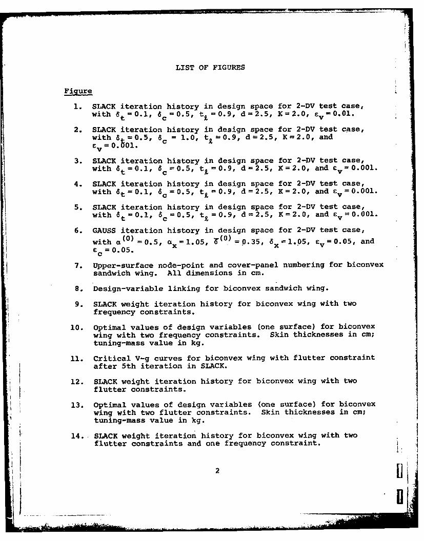
1. SLACK iteration history in design space for 2-DV test case,with 6t=0.1, 6c =0.5, tt =0.9, d=2.5, K=2.0, ev=0.01.

2. SLACK iteration history in design space for 2-DV test case,with 6 =0.5, ac = 1.0, tI=0.9, d=2.5, K=2.0, andCv = 0.b01.

3. SLACK iteration history in design space for 2-DV test case,with 6 t= 0 . 1

, c =0.5, tz=0.9, d=2.5, K=2.0, and Cv=0.001.

4. SLACK iteration history in design space for 2-DV test case,with St=0. 1 , 6c=0.5, t9=0.9, d=2.5, K=2.0, and cv=0.001.

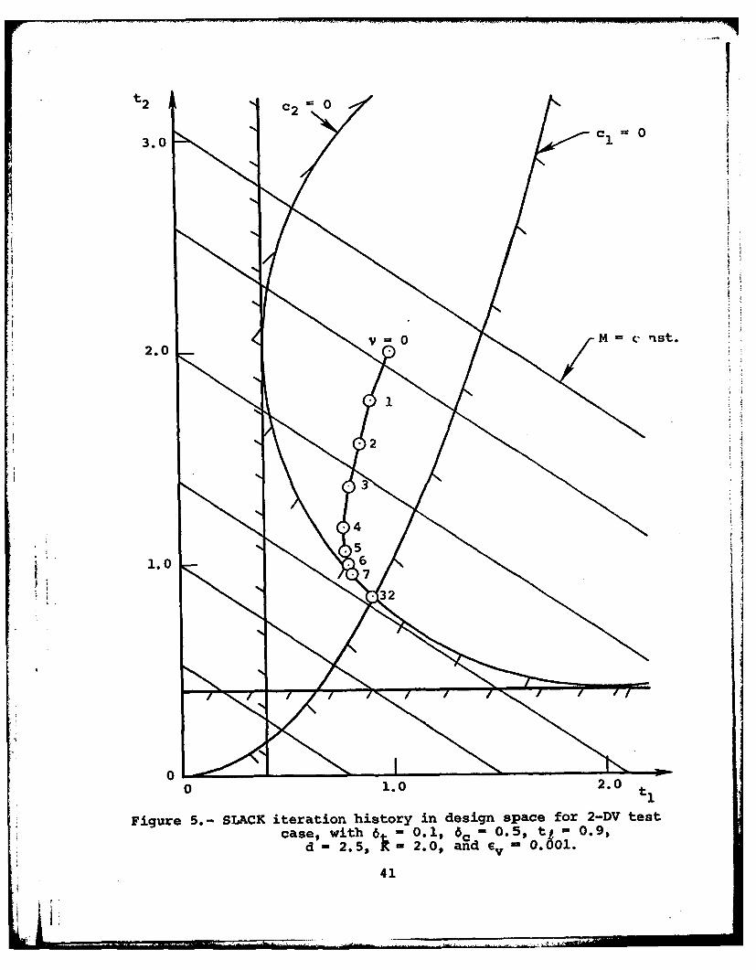
5. SLACK iteration history in design space for 2-DV test case,

with 6 t=0.1, 6c=0.5 , tz=0.9, d=2.5, K=2.0, and cv=0.001.

6. GAUSS iteration history in design space for 2-DV test case,()= 0. 5(,03, x " 5 .5 nwith a(0) 0.5, x =1.05, = -0.305, =1.9 5, andc =0.05.c

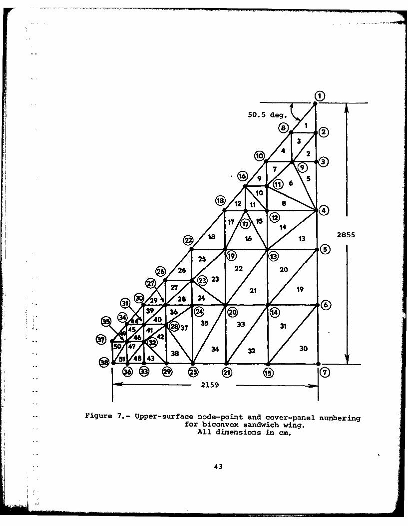
7. Upper-surface node-point and cover-panel numbering for biconvexsandwich wing. All dimensions in cm.

8. Design-variable linking for biconvex sandwich wing.

9. SLACK weight iteration history for biconvex wing with twofrequency constraints.

10. Optimal values of design variables (one surface) for biconvexwing with two frequency constraints. Skin thicknesses in cm;tuning-mass value in kg.

11. Critical V-g curves for biconvex wing with flutter constraintafter 5th iteration in SLACK.

12. SLACK weight iteration history for biconvex wing with twoflutter constraints.

13. Optimal values of design variables (one surface) for biconvexwing with two flutter constraints. Skin thicknesses in cm;tuning-mass value in kg.

14. SLACK weight iteration history for biconvex wing with twoflutter constraints and one frequency constraint.

3 2I 1;

.. .. . . ... I

LIST OF FIGURES (Concluded)

* - Figure

15. Optimal values of design variables (one surface) for biconvexwing with two flutter constraints and one frequency constraint.Skin thicknesses in cm; tuning-mass value in kg.

3

AEROELASTIC OPTIMIZATION WITH

MULTIPLE CONSTRAINTS

1. INTRODUCTION

This report summarizes the work performed under the sponsor-ship of the Air Force Office of Scientific Research, with Contract

No. F49620-78-C-0105. The overall goal of this research has beento develop improved methods of designing least-weight aerospace

structures that satisfy both strength and stiffness requirements.

During the first year, some efficiency comparisons wereundertaken with a number of different optimization algorithms.All of these algorithms were applied to problems involving asingle behavioral constraint. This work is summarized in reference 1.

From this work, two algorithms were chosen for work with multipleconstraints. The first algorithm is an extension of work performed

by Segenreich and co-authors (refs. 2-4). The idea here is toemploy slack variables in order to transform the usual inequalitybehavioral constraints into equality constraints. In this manner,

an optimization algorithm based on multiple equality constraintscan be applied. Such an approach has been applied to problems

with static constraints in reference 4.

The second algorithm was developed by Rizzi (ref. 5). This

algorithm employs a Gauss-Seidel iterative procedure to aid inthe elimination of inactive constraints. It has been applied by

Rizzi in reference 5 to problems involving both strength andstiffness constraints, and it was felt desirable to use it forcomparison with the first algorithm on larger problems. Since

both of the algorithms discussed above employ a similar resizing

formula, the comparison proposed is primarily a test of twodifferent procedures for handling multiple constraints.

The sections that follow will describe in detail the twoalgorithms as coded here, the numerical applications carried out,

and some recommendations for future work.

4 [

~2. STATEMENT OF PROBLEM AND THEORETICAL BACKGROUND

Consider the problem of minimizing the total mass MT of

a structure. Let the design variables be ti , i =1,2...,M,

which may either be member-sizing variables in a finite-elementmodel of the structure or concentrated-mass sizing variables.

With the usual types of finite elements, the mass is a linear

function of the design variables, and the total mass can be writtenas

MmT= Mo + a ait i

where M is the mass not available for optimization, such as

fuel mass. There are behavioral constraints on the structure,representing strength or stiffness requirements such as maximumallowable stresses, minimum frequencies of free vibration, maximumdisplacement, or minimum flutter speeds. These are characterized

as inequality constraints

c.(t.) < 0, j = 1,2# ......,N (2)

Finally, there can be side constraints that define the

*maximum and minimum values of the design variables:

(ti)min_- t i _< (ti)max, (3)

Necessary conditions for a local minimum are given by theKuhn-Tucker conditions. These can be written in the form

N ac.vi ai + I Xj 7)i 0, < t (4)

j=l ati i min- i- (timax

o , t. = (t) (5)

vi < 0 , t. = (t.)max (6)

5 m

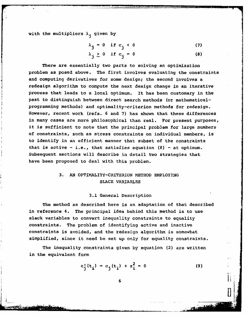
with the multipliers .j given by

Xj = 0 if c. < 0 (7)

X > 0 if c. =0 (8)

There are essentially two parts to solving an optimization

problem as posed above. The first involves evaluating the constraintsand computing derivatives for some design; the second involves a

redesign algorithm to compute the next design change in an iterativeprocess that leads to a local optimum. It has been customary in the

past to distinguish between direct search methods (or mathematical-

programming methods) and optimality-criterion methods for redesign.

However, recent work (refs. 6 and 7) has shown that these differences

in many cases are more philosophical than real. For present purposes,

it is sufficient to note that the principal problem for large numbers

of constraints, such as stress constraints on individual members, is

to identify in an efficient manner that subset of the constraints

that is active - i.e., that satisfies equation (8) - at optimum.Subsequent sections will describe in detail two strategies that

have been proposed to deal with this problem.

3. AN OPTIMALITY-CRITERION METHOD EMPLOYING

SLACK VARIABLES

3.1 General Description

The method as described here is an adaptation of that described

in reference 4. The principal idea behind this method is to use

slack variables to convert inequality constraints to equality

constraints. The problem of identifying active and inactive

constraints is avoided, and the redesign algorithm is somewhatsimplified, since it need be set up only for equality constraints.

The inequality constraints given by equation (2) are written

in the equivalent form

c!(t) c.(t.) + z2= 0 (9)

6

K JAM

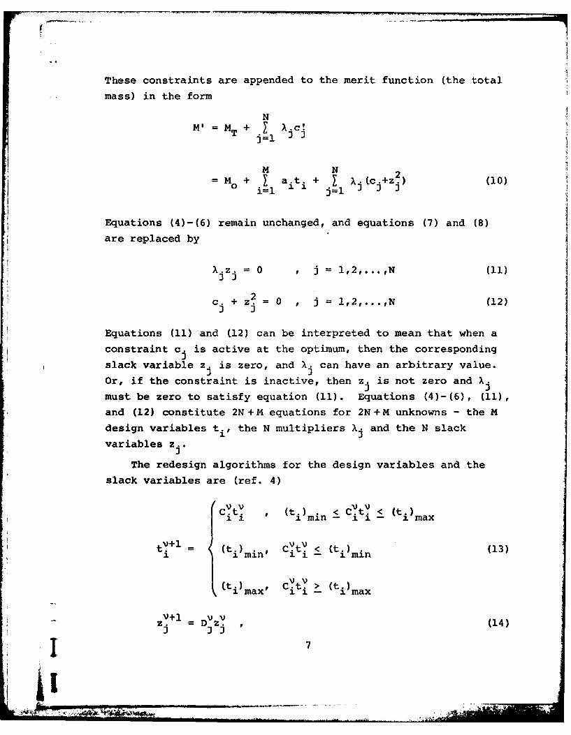
These constraints are appended to the merit function (the total

mass) in the form

NM, M + 1 c

M N 2b4 + ait i + Aj(c.+z.) (10)1 j=1 1 j

Equations (4)-(6) remain unchanged, and equations (7) and (8)

are replaced by

X.zj = 0 , j l,2,...,N (11)

c. + Z = 0 , j -- ,2,...,N (12)I J

Equations (11) and (12) can be interpreted to mean that when a

constraint c. is active at the optimum, then the corresponding)slack variable z. is zero, and X i can have an arbitrary value.

Or, if the constraint is inactive, then z. is not zero and X.J )must be zero to satisfy equation (11). Equations (4)-(6), (11),

and (12) constitute 2N+M equations for 2N+M unknowns - the M

design variables ti, the N multipliers X. and the N slack

variables z..

The redesign algorithms for the design variables and the

slack variables are (ref. 4)

C VtY (t. V ctY < (t)i( imin- i i- (timax

i i min' I i min (13)

(t.) Citi > (t.)imax i i - imax

z. D , (14)

7

k"

IA~'

where v is the iteration number and

a+a 1 a. X (15)

VDY = 1 + (a -)KX' (16)

The redesign factor C is the same as that proposed by Kiusalaas1

(ref. 8). From the optimality criterion, equation (4), it can

be seen that CV approaches unity, independently of the value ofi

the relaxation parameter a , as the optimum design is approached.

From equation (11), it can be seen that the factor D approaches

unity in similar fashion as the design converges. The constant K

is a free parameter that can be selected by the designer; in effect,

it permits controlling the step size on the slack variables

differently from the step size on the design variables.

To find the Lagrange multipliers X, the requirement thatJJc! = 0 for all j is imposed. This is equivalent to the procedure

employed in an optimization problem with multiple equality constraints,

except that there are some additional terms involving the slack

variables. Also, for the sake of completeness, terms will be

included to account for design variables that are reaching their

upper or lower bounds. As a design variable reaches one of these

bounds, it is left at the appropriate value and relegated to the

passive set. After a converged solution has been obtained, tests

based on equations (5) and (6) are applied to see if any passive

variable is to be reintroduced to the active set.

Now let AV denote the active set of design variables, andvassume that at the vth iteration equations (13) have been applied,

and those design variables that are going into the passive set

(not those relegated to the passive set from a previous iteration)have been identified. Let P£ and P V denote such design variables

for the lower (or minimum-value) and upper (or maximum-value)

bounds, respectively. Then,

8

7,V

(&-1)Y = ( [ 'N a/c.V]vSj=1 )~at~ ji v C

Vt (V t cV (17)i min I

To first order,

(Ac')" ACV~ + ZYAzY (18)

and

Ac' =(~)Ati ic(A +Pv+P) (19)

After use of equations (17) for At i', equation (19) becomes

Ac. (ct -1) 0. + N 0 V X + ~.~ac.) (

\) k=1 k ieP p 1 1 m

IVP t1L max- ii

where

-' Y) tY

ij eAv a.i atiJ t 1(2

9

Equations (14) and (16) yield

Az. = (a-l)Kxvz (23)

Equations (20) and (23) can now be combined to give an expression

for (Ac')v. Setting this quantity to zero for all j, letting2 v I

a

(zj) =-c , and rearranging the resulting equations gives a

linear set of equations for the Lagrange multipliers X.:

N -

kj k i I (ac' V[ti..-tYi]

ac.

/ c. \Vr

+ 1 -1 (V at. ( ( ) (4

u

where

kj = kj 2Kc kj (25)

and 6kj is the Kronecker delta function.

Choosing the step-size parameter (a V-1) completes this

algorithm. There are four criteria that are applied; these follow,

with slight modifications, the criteria set forth in reference 4.

The criteria are as follows:

(i) Limit on step size.

The change in each design variable is given by

AtO = (av-l)viti, (26)

where v. = vi/ai. The magnitude of the vector whose components

i1 111 10

j---------

are Ati/ti is

I ---bt- v I VlI ( 2)v]1/2 (27)

If 62 is now defined as the maximum permissible magnitude ofhti/ i, then the left-hand side of equation (27) is 6t(NA)1/2

where N A is the number of design variables in the active set.

Equation (27) can then be rewritten as a limiting criterion on

*~V /2 IV- ItN)"/X (v?\)11/2Ia- .i (N (28)Iv l v

(ii) Feasibility of the new design.

This criterion is applied in order to ensure that a design

that is near a constraint boundary c. =0 will not be driven too)far from it. Equations (12), (18), and (23) can be combined

for (Ac!)V= 0 to give to first order

Ac . = 2(a'-1)KXYc , (29)

With 6 defined as the maximum allowable value of IAc!/cI,c )equation (29) becomes

V-1 < 6 /2KIX'.l (30)-c j

(iii) Bounds on the design variables.

This criterion is used to ensure that no design variable is

driven too far outside its allowable range. Tolerance bands on

the upper and lower bounds are established with parameters t u(>l)

and tt (<l), respectively. With the proviso that (a'-1) be always

negative, this criterion takes two forms. From equation (26),

~11

b _ _ _ _ _ _ _

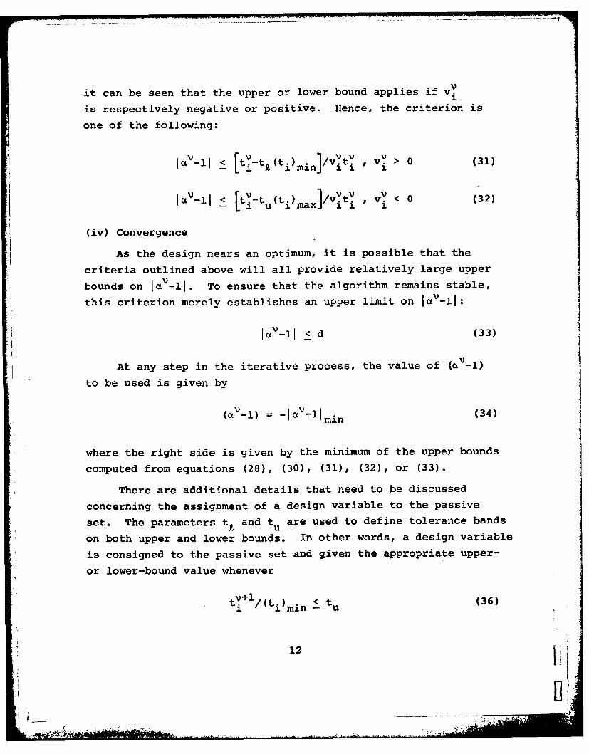
it can be seen that the upper or lower bound applies if v.:

is respectively negative or positive. Hence, the criterion is

one of the following:

avl [tt (t) v V1 > 0 (31)V-lj k t-t(t)mi n /viti I

imax I Vi v. < 0 (32)L1u max1/viti i

(iv) Convergence

As the design nears an optimum, it is possible that the

criteria outlined above will all provide relatively large upper

bounds on lIt-lI. To ensure that the algorithm remains stable,

this criterion merely establishes an upper limit on lo-ih:

IsV -1 d (33)

At any step in the iterative process, the value of (a -1)

to be used is given by

(V 1-l) =mi n (34)

where the right side is given by the minimum of the upper bounds

computed from equations (28), (30), (31), (32), or (33).

There are additional details that need to be discussed

concerning the assignment of a design variable to the passive

set. The parameters t£k and tu are used to define tolerance bands

on both upper and lower bounds. In other words, a design variable

is consigned to the passive set and given the appropriate upper-

or lower-bound value whenever

Sn+l tu

12

I__

or

v+li (ti max- t£ (37)

It is intended here to accelerate as much as possible the selec-

tion of active and passive variables. When tu and t£ are not

equal to unity, this means that a design variable may be selectedVas passive, even though (a -1) has not been selected from equa-

tions (31 or (32). As a consequence of this, either of theV Vsets P or P will no longer be null, and it will be necessary

to return to equation (24) and repeat the calculation of the

Lagrange multipliers. In principle, this process must be repeated

until the selection of the passive variables converges; in

practice, only one repetition is usually necessary. Note also

that if t. and tu are set equal to unity, then the choice of

(a-l) will be governed by one of the equations (31) or (32) and

no repetition will be needed, since there is no inconsistency inequations (17), which give the increments At.

1

Since all of the a. 's are positive, convergence to a local1

minimum is measured by the vi , and the convergence criterion is

IIvI C ieA~ (38)

where cv is a user-supplied quantity. To ensure that no passive

design variables need to be reintroduced into the active set, the

applicable Kuhn-Tucker conditions, equations (5) and (6), areverified (with v. rather than v.):

1 1

V -Vv > 0 , (39)

V -- Vv. < 0 icP (40)I- u

13

Here and PO define the complete set of passive design variables.

Since the redesign formula gives equation (26) for At? , there1

is an obvious physical explanation for the above conditions. Ifa design variable t. is at its minimum value and its associated

1

convergence function vi is negative, a redesign will produce apositive increment Ati, thereby implying that this design variable

should be reintroduced into the active set. Similar reasoningholds for a design variable at its upper bound when its conver-

gence function is positive.

3.2 Summary

The algorithm is summarized in the following steps%

(1) For the current design, evaluate the constraints c., j =,2,...,N.

(2) Calculate the derivatives ^c/ati , i=l,2,...,M; j =1,2,...,N.

(3) Calculate 8. from equation (21) and 0-kj from equations (22)

and (25).

(4) Solve for the X from equation (24), with P£ and Pu nullif this is the first time the multipliers are calculated for

this iteration. If not, include terms for the appropriate

design variables identified in step (8) below.

(5) Compute the convergence functions vi = i/a ; is given by

equation (4).(6) Test for convergence, using equation (38). If this test is

satisfied, test the passive variables with equations (39) and

(40). If any of these tests fails, redefine the active and

passive sets appropriately and return to step (3). If the

tests are satisfied, exit with the final design information.

(7) Compute (a V-l) from equations (28) and (30)-(34).

(8) Compute the new design variables according to the first of

equations (13) and equation (15). Test for new passivevariables using equations (36) or (37). If necessary, redefine

the active and passive sets and return to step (3). Other-

wise, compute the new mass and return to step (1) to begin anew iteration.

14

I

In brief, this algorithm seeks to avoid identifying active

constraints by using slack variables to permit all of the constraints

to be treated as equality constraints. Implied in this approach

is the assumption that all intermediate designs and the starting

design must be feasible - that is, no constraint violations aretolerated. Also, all constraints are to be evaluated at every

design, as the algorithm is currently formulated. For truly large

systems, where a great number of constraints may be applied, itwould be necessary to introduce a "throwaway" concept or some

similar strategem, whereby constraints that are nowhere near being

active are at least temporarily ignored.

4. AN OPTIMALITY-CRITERION METHOD EMPLOYING

GAUSS-SEIDEL ITERATION

4.1 General Description

This method is based on the work of reference 5. The stra-

tegy here is to let the active constraints be selected by the

signs of the Lagrange multipliers. The Gauss-Seidel iterative

procedure is used to permit the constraints associated with

negative multipliers to be eliminated efficiently. At the optimum,

the only constraints involved are the active ones, for which theLagrange multipliers are non-negative.

The problem statement is given by equations (l)-(8), with

the redesign algorithm given by equations (13) and (15). In order

to reduce the number of constraints included in the calculation

of the X., a positive tolerance parameter WV is specified, and

those constraints are selected for which

c.> (41)j c

Let AV define the set of constraints for which this test is satis-cfied. These constraints are either potentially active or violated.

15

Computation of the first-order approximation for Acj givesJ

equation (20). If it is now assumed that all the constraints inAV are to be active constraints, then it is required thatcvC = -cY , and equation (20) can be manipulated to give

/Vc. V a

IV Ok Ak (42) V(a ) imi

Th ceficens and are given by equations (21) and (22)respectively, with J'kCc" frwih!

V

The next step is to determine that subset of Ac o hcSsolutions of equations (42) will produce non-negative values of

Ve V F

Ak. One approach is to solve equations (42) for the set of Ac

eliminate the terms associated with any negative multipliers,and repeat this process until only non-negative values of the

multipliers are computed. However, as noted in reference 8, there

is no quarantee that this procedure will converge, because of thecoupling among the equations provided by the coefficients 0k # j. The solution proposed in reference (5) is to apply the

Gauss-Seidel iterative procedure to equations (42). Let these

equations be rewritten in matrix form as

[B]{x} = {b} (43)

and let n be their order. Then, let equation (43) be recast in

the following form:

{A = [B]{Xl + {b} (44)

16,It:

where

Bij = Bij/B.. - 1 , i,j =1,2,...,n (45)

b. = bi/Bii , i=l,2,...,n (46)

Thus, [B] is a matrix with a zero principal diagonal, and the

Gauss-Seidel iterative algorithm is

i-inB. X + j B X-l + bi , i=l,2,...,n (47)

j=1 1)) j=+i ij 1

Here j is the Gauss-Seidel iteration number, and the terms in the

first summation for i = 1 and the second summation of i =n are

ignored. As this algorithm is applied, each multiplier Xk is

estimated from current values for i < k. This means that when-

ever a negative value for a multiplier is determined, it can be

immediately deleted, with minimal impact on the values computed

for the remaining multipliers in that particular iterrtion.

Although it cannot be rigorously proven, this process is expectedVto lead naturally to the proper subset of A (ref. 5). Let thisc

subset be A .Redesign can now be carried out with equations (13) and (15),

with jeA in equation (15). The process of identifying passivecdesign variables is similar to that described in Section 3 above.

If any design variables are predicted to reach their upper or

lower bounds, then the calculations of the multipliers must be

repeated, with the appropriate terms added to equation (42).

Unlike the original algorithm proposed in reference 5, design

variables remain passive until a converged design is found. At

that point the tests given by equations (39) and (40) are applied,

and the appropriate variables reintroduced into the active set if

any of the tests fails.

17

The parameters a and 6 are scheduled as follows:

aV v x-i (48)

if a T -l (49)C XC

To accelerate convergence, a can be chosen as a positive number

greater than unity, with a 0 given as a negative number. The

multiplier 6x is typically less than unity, since it is desirable

to have equation (41) provide an increasingly restrictive test as

the optimization proceeds.

Convergence is measured by two criteria:

-cvj < c jA c (50)c C

V < " , ieAV (51)

4.2 Summary

This algorithm is summarized as follows:

(1) For the current design, evaluate the constraints cj,

j =1,2,...,N.(2) Calculate the derivatives ac /Bti , i=l,2,...,M, J=1,2,...,N.

(3) Use equation (41) to test for the set Ac of potentially active

or violated constraints.

(4) Compute 'and from equations (21) and (22), respectively,

with j v kj

(5) Use the Gauss-Seidel iterative formula, equation (47) to deter-

mine the constraint set Ac.

(6) Compute the redesign factors C from equation (15) and identify

18

any new passive variables, redefine the active and passive

sets accordingly and return to step (4), with the appropriate

terms added in equation (42). Continue this loop throughsteps (4)-(6) until there is no change in the active-passive

identities.(7) Compute the convergence functions v. for the constraint set

-v 1A and test for convergence with equations (50) and (51).

If these tests are satisfied, test the passive variables with

equations (39) and (40). If any of these tests fails, redefine

the active and passive sets accordingly and return to step (4).

If not, exit with the final design information.

(8) If any of the convergence tests fails, compute the new design

variables (equations (13)) and the new values of the step-size

parameter a and the constraint-tolerance parameter 6c(equations (48) and (49)) and return to step (1) to begin anew iteration.

It is worth noting that this algorithm also requires that all

constraints be evaluated at each iteration. The selection of the

active constraints - that is, those that are actually included in

the redesign - is a two-stp process. First, the constraints that

are violated or are within a given tolerance band around zero are

chosen, and from these the active set is chosen by eliminating

those for which the multipliers are negative. It is therefore to

be expected that this strategy would be most valuable when there

is a large number of constraints, and the active set is rapidly

changing from iteration to iteration. When the constraints are

so numerous that it is not feasible to evaluate them all at every

iteration, a "throwaway" concept would be useful and could easily

be incorporated.

5. CONSTRAINT EVALUATIONS AND DERIVATIVE CALCULATIONS

Three types of constraints are considered - displacement in

response to a fixed static load, natural frequencies, and flutter

19

speed. The evaluations of the constraints and their derivatives

follow generally the procedures outlined in reference 1. The

basic formulas will be repeated below for the sake of completeness

and any differences between current usage and that in reference 1

will be described.

5.1 Displacement Constraint

The constraint is given by

u-r (52)

(Ur) des

and the derivative is calculated by the dummy-load method:

S I au r I(ri ui[K.i u } (53)

(Ur) des 1 (Ur) des

Here {ul is the set of nodal displacements associated with a given

loading condition, whose rth component ur is constrained to be less

than or equal to (ur)des , and {u(r), is the set of displacementsresulting from the application of a dummy load at the rth node in

the direction of ur. The matrix [Ki] is the stiffness matrix

associated with design variable ti; both mass and stiffness

matrices vary linearly with the design variables. For multiple

constraints, different loading conditions, and different displace-

ments for each loading condition, can be considered.

5.2 Frequency Constraints

In contrast to the expression in reference 1, the constraint

function for a natural-frequency constraint is written as

c 1 r (54)( r) des

20

77H

r

- - -

where w is the rth free-vibration frequency of the structure, and

it is constrained to be greater than or equal to (w )des

The derivative expression is

c . 1 rat.t.(55) W r) des

where

(r) 2 (r) q(r)a 3r Iq r J [SKi]{qr) r Lrq J [G i]{q (54

a-t- ~i 2wr Iq (r) ][GM]{q (r)5

It is assumed here that the natural modes of the initial design

are used to define generalized coordinates for all the designs, so

that the generalized derivative matrices [GK i] and [GM i] can be

written as an inactive part plus the sum of the active parts.

The column {q(r) is the rth mode shape of the current design

(see reference 1). Multiple frequency constraints can be considered.

5.3 Flutter-Speed Constraints

Here, the constraint function c is identified directly with

the damping parameter g. In essence, this formulation requires

that the imaginary part of a critical root of the flutter equations

be non-positive at a given free-stream speed and altitude. The

mode shapes of the initial design are used to define generalized

coordinates, so the generalized derivative matrices [GK i] and

[GM.] are constant, and the generalized aerodynamic matrix [GA]varies only with reduced frequency k. The derivative is evaluated

21

-I

just as in reference 1:

ac = 2 i + bW 3

i R R1 gI2gR 21at a 2 1 2 3 V 4)

- (R - 2R( I I + gR2 /D (57)

where

D = (2R 3 + 213 + 1 14 )13 + (2R3 -2g1 3 bw )R (58)

= Re(lpj[GMi ]lgq) (59)

R2 Re(tpI[GKi ] q) (60)

R3 = Re (LPJI [GK]t g.}) (61)

aGA .-R= Re(Lpi [ - Iq 1) (62)

and It, I2, 13, and 14 are corresponding imaginary parts. Also,

V is the free-stream speed, b is a reference length, w is the

frequency, {Lq1 is the eigenvector for the critical flutter mode,

and (p) is the adjoint eigenvector.

When the constraint is evaluated, it is necessary to ensure

that the reduced frequency, which is fixed in order to evaluate

[GA], is compatible with the frequency computed from the eigenvalue

= (l+ig)/w 2 (here i= (-l)1/2). While it is possible to computea_ nd use it to estimate the new value of the frequency once theatidesign change has been compuated, it is simpler to iterate. The

previous value of reduced frequency is used to define the aero-

22

------------------------------------j1;j110

dynamic matrix [GA], and a value of w computed from the eigenvalue

?r. If this value is not equal to within some specified tolerance

to the value used to compute the reduced frequency, it is used as

the new reduced frequency and the matrix equation for flutter is

solved again. Typically only a few iterations are needed; more

details can be found in reference 1.

Multiple flutter-speed constraints may be considered. These

may be critical speeds at different altitudes or Mach numbers, or

they may involve additional potentially critical branches for a

single case.

5.4 Accuracy of Derivative Calculations

In order to test the accuracy of the derivative calculations,

the analytical derivatives, computed as described above for

frequency and flutter constraints, were compared with derivatives

computed by finite differencing. The structure used was the

sandwich wing of reference 9. This wing had a primary flutter

constraint corresponding to M.=0.8 at an altitude of 2,438 m,

a secondary flutter constraint corresponding to the crossover of

another root in the V-g plane at a slightly higher airspeed, and

a frequency constraint that required the fundamental natural

frequency to be not less than that of the initial design. Addi-

tional details concerning this wing and the constraints are given

in Section 6.

Finite-difference derivatives with respect to all seven design

variables are compared to analytical derivatives in Table 1. These

derivatives were computed at an intermediate design obtained from

an optimization run, so the modes used to define generalized coor-

dinates are primitive modes. As can be seen, the derivatives

calculated by the two methods are generally in very good agreement.

Finite-difference derivatives were computed for a number of different

perturbation magnitudes and compared in order to minimize numerical

errors; the derivatives given in the tables were determined with

5% perturbations.

23

h __ __

During this portion of the study, it was discovered that the

convergence test used in the iterating to determine the new frequency

when the flutter constraint was being evaluated had to be tightened

considerably in order to ensure sufficiently accurate determination

of the damping parameter g. It was ultimately necessary to require

that the selected and computed values of reduced frequency agree

to within 0.0001.

As noted in reference 10 and elsewhere, the use of fixed modes

does lead to inaccuracies both in constraint evaluation and in

derivative calculation. On the other hand, updating the modes

after every iteration, or even after a certain number of iterations,

is often not feasible because of the additional computer time

required or the abrupt changes introduced in constraints and

derivatives when the modes are changed. In principle, using a

sufficiently large number of modes, even if they are used as

fixed modes, should resolve this difficulty. However, there are

practical limits to the number of modes that can be used. For

example, mode shapes are often fit with polynomials or splines

before they are used in calculating generalized aerodynamic forces,

and the accuracy of such fits for high-order modes with complicated

node-line patterns is questionable.

Another approach has been proposed in reference 5. It was

hypothesized that the principal source of modeling errors with

fixed modes is the failure of the inplane portions of the modes

to produce negligible inplane forces as the design is changed.

To avoid this problem, it was proposed to preserve unchanged the

transverse displacements but recompute the inplane displacements

from the requirement that the inplane forces be zero. This would

involve additional computations in constructing the generalized

mass and stiffness matrices but would not affect the generalized

aerodynamic forces. In reference 5, the inplane displacements

were recomputed, but the additional terms that arise in the

derivative calculations to account for changes in certain portions

24 f0

An

of the modes were ignored. The accuracy of constraint evaluation

was enhanced by this strategem, and it is expected that accounting

for the mode-shape changes in the derivative calculations, which

involves only the derivatives of the generalized mass and stiffness

matrices, should improve the accuracy of the derivative calculations

with little added computational effort.

6. NUMERICAL EXAMPLES

6.1 Test Cases

It is instructive to consider first some test cases involving

two design variables, so that the progress of the optimization can

be plotted and visualized in design space. For all of the test

cases, the merit function was

M = 2t1 + 3t2 (63)

For the first test case, the "behavioral" constraints were

c I = t 2 -t < 0 (64)

1 2 2

C2 = 1- (t2 + t2)/2 < 0 (65)

and minimum-gage constraints of (tl)min = 0.2, (t2)min= 0 . 5 were

also imposed. Figure 1 presents the path in design space taken

by the slack-variable program (program SLACK) from an initial

design at (2.0,1.5). As can be seen the first few steps follow

reasonably closely a steepest-descent path, nearly normal to the

M =const. lines, until the minimum-gage constraint on t2 is

encountered. Thereafter the designs proceed along this constraint

boundary until the intersection with the c2 = 0 boundary is reached,

I at (1.3228, 0.5000). The value of the merit function at this point,

25

T . ..... w

which also is a global minimum( is (M)min =4.1456. After 42 itera-

tions, the computed values for the optimum were CM)min =4.1460 at

(1.3230, 0.5000). Values of other parameters used in SLACK are given

in the caption. No attempt was made at this point to vary these

parameters so as to reduce the number of iterations required.

The next set of slack test cases was run with the sign on c

changed, so that the feasible domain was to the left of the c1 = 0boundary. With the same minimum-gage constraints, there are multiple

extrema here - one at (0.2000, 1.4000), with (M)min= 4.600, and one

at (1.0000, 1.0000), with (M)min =5..000. With the initial design at

(0.9000, 1.2000), the latter extremum is found after 44 iterations

(figure 2); the computed values are (M)min=5.0019 at (0.9981, 1.0020).

If the initial design is moved to (1.2000, 2.000), the other extremum

is found after 64 iterations (figure 3). The computed values here

are (M) min =4.6006 at (0.2000, 1.4002). In figures 2 and 3, a line

is drawn through the origin in the steepest-descent direction. The

intersection of this line with the c2 =0 boundary (point A) definesthe maximum value of M on the boundary. It is therefore readily

apparent that any optimization step reaching the c2 =0 boundary to

the right of point A will result in an optimum solution to the right,

and in similar fashion the optimum to the left will be found for any

step reaching the c2 =0 boundary to the left.

Another test case with the same constraints cI and c2, but with

(til)min =0.500, (t2)min =1.500, was run to test the operation ofSLACK when the optimum design is dictated by the minimum-gage

constraints. This optimum was found after 17 iterations (figure 4).

The final SLACK test case involves two concave constraints -

the same constraint function cI used above, and

= (ti-2)2 + (t2-2)2 - 2.56 < 0 (66)

Minimum-gage constraints of (0.4000, 0.4000) were imposed, but

these were inactive, and the global optimum is at (0.9102, 0.8285),

26

with (M)min =4.3060 (figure 5). With an initial design of

(1.000, 2.000), the optimum was found after 32 iterations. The

computed values were (M) mi=4.3084 at (0.9072, 0.8313).

It is interesting to note that the behavior of the slack-variable algorithm, as given by the paths in design space plotted

for these test cases, closely follows a gradient-projection

strategy: steepest descent until a constraint surface is encountered,and then steps along the projection of the gradient of the merit

function on the tangent to the constraint surface (see, for example,

reference 11). This is not so surprising, in view of the close

relationship between a Kiusalaas-type algorithm and a projection

algorithm (reference 12).

A number of cases with different parameters in SLACK were

run with the constraints and initial design given in figure 5.

The results are summarized in Table 2. As would be expected,

imposing a more severe convergence criterion results in an

increased number of iterations required - in this case, the number

of iterations is almost doubled for a factor of 10 reduction in

Cv. Comparing numbers of iterations with different values of K

and 6c suggests that larger values of 6c and smaller values of

K will enhance convergence, at least in cases where many iterations

take place along a nonlinear constraint boundary. This is in fact

expected to occur for most problems of practical significance.

One test case was run with the program based on Gauss-Seidel

iteration - program GAUSS. This case involves the same merit

function as previously used and three constraints:

2c t2 t2 <0 (67)

c -1 + (t2 + t2)/2 < 0 (68)

C 2(_2 _ o3 =21 -t 2 (69)

27

These constraint boundaries and the results from a run with program

GAUSS are presented in Figure 6. The feasible domain is a closed

area roughly triangular in shape, with a global optimum at the

intersection of the boundaries of the two active constraints, c1

and c3 . The optimum is at (0.8165, 0.6667), with (M)min =3.6330.

With an initial design at (0.8200, 0.9300), the optimal solution

was found in just four interations to be (M)mi =3.6718 at

(0.8115, 0.6830). As can be seen in the figure, there were some

oscillations about the optimum. These were undoubtedly the result

of the values used for the various parameters, which are given

in the caption. Note in particular that a tighter convergence

test would have located the computed minimum closer to the exact

one. No studies of the effects of variations in these parameters

were performed at this time, since it was decided to concentrate

the remaining efforts on more complicated problems with program

SLACK.

6.2 Biconvex Sandwich Wing

The structure chosen for the remaining examples was the

biconvex sandwich wing of reference 9, example 2. A planform

view of this wing is given in figure 7, which shows the node-point

and cover-panel numbering. The coordinates of the nodes are given

in reference 9. To model the core, thick shear webs were placed

along each chordwise and spanwise line between node points, and

axial elements were placed between upper-surface and lower-surface

node points, except at the wing root. These elements were used

to contribute stiffness only. Triangular cover panels, numbered

as indicated in figure 7 for the upper surface, were used to model

the skin. The complete model had 76 nodes, 14 of which were

restrained at the root; 102 cover elements; 49 shear webs; and 31

axial elements. There were 186 unrestrained degrees of freedom,

which were collapsed to 31 transverse degrees of freedom at the

upper surface. The design variables were taken to be the thicknesses

of the cover panels. Each design variable governed the thickness

28 [

of an upper cover panel and its lower-surface counterpart, so

there were a total of 51 design variables, which could be

additionally linked in any combination to create smaller problems.

Concentrated tuning masses were also located at nodes 18 and 56;

these were controlled by a single additional concentrated-mass

design variable. Finally, nonactive concentrated masses were

located at all the nodes to represent internal fuel. The values

used for these masses were obtained by subtracting the active mass

contributed by the cover panels from the total node-point masses

given in reference 9.

Material properties for the cover and web elements were the

same as those given in reference 9: E=1.1308 x10 kPa,

p =4.4244 x 10- 6 kg/cm 3 , and v=0.3 for the covers; and

G = 4.3492 x 107 kPa and =0.3 for the webs. The axial elements,

which had no counterparts in the model of reference 9, had4 2

EA= 2.1440 x 10 kPa-m2 . These elements were needed in the presentmodel to stabilize the shear webs, which were different from the

webs used in reference 9. It should be noted that the webs and

axial elements were used to provide an extremely stiff, weightless

core. As long as these elements are stiff enough, the transverse

mode shapes and frequencies of the wing will not be very sensitive

to the values used for these stiffnesses. The webs were all

assumed to be 9.8 in. thick, and the cover panels were sized

according to the initial design of example 2 in reference 9-

0.2540 cm for panels 1-43 and 52-94, and 0.05080 cm for panels

44-51 and 95-102. The initial weight for this wing was 67,000 kg,

including the fuel, with 7,602 kg available for optimization

This includes 350.3 kg for the tuning masses.

In the examples that follow, the design variables were

linked as indicated in figure 8, so that the number of design

-* variables was reduced to seven, including the concentrated-mass

design variable (no. 7).

29

! .-- --

6.3 Optimization with Frequency Constraints

Mode shapes and frequencies were computed for the wingdescribed above, and the wing was then optimized by program

SLACK with the requirement that the first two natural frequenciesbe greater than or equal to 6.20 Hz and 18.70 Hz, respectively.

The corresponding frequencies of the initial design were slightly

in excess of these values. The first 12 modes of the initialdesign were used as fixed modes to define generalized coordinates.

After 34 iterations, an optimum weight (less fuel) of 569.9 kg

was computed. An iteration history of the variable weight is

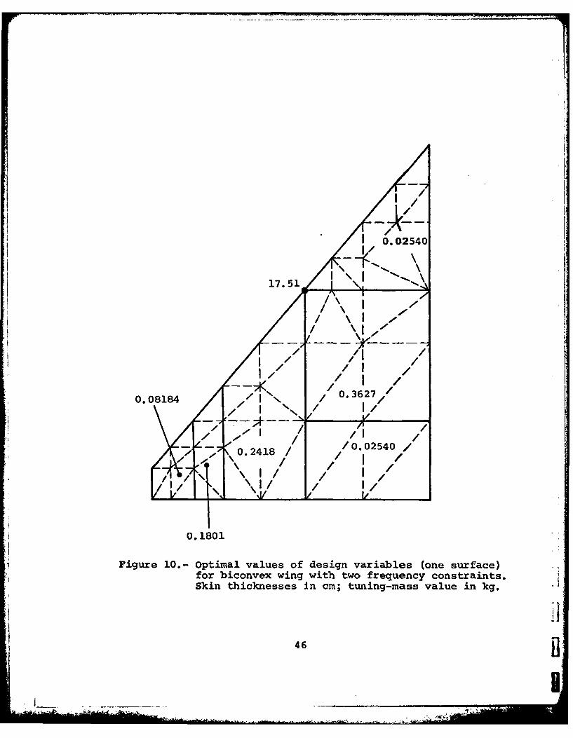
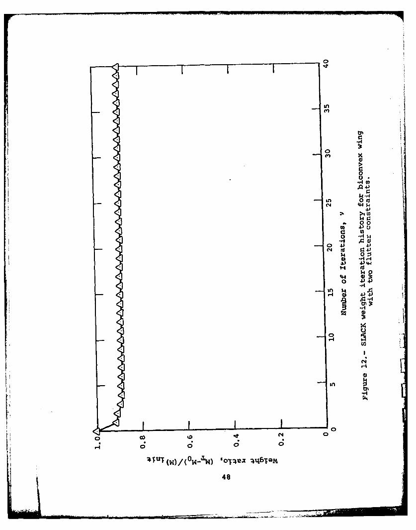
presented in figure 9, and the optimal values of the designvariables are presented in figure 10. Around 25% of the weight

available for optimization was removed. Both frequency constraints

were active at the optimum, as would be expected. CPU time

required on an IBM 370/78 computer was approximately 0.1 sec per

iteration. Parameters used in SLACK were 6t 6c = 0.5, t= 0.9 ,d = 2.5, K=0.1, and -v = 0.001. Minimum values of 0.02540 cm were

specified for design variables 1-5, while design variables 6 and

7 had minima of 0.01016 cm and 35.03 kg, respectively.

The iteration history of figure 9 demonstrates the usualrapid reduction in weight, followed by relatively small weight

reductions as the optimum solution is approached.

6.4 Optimization with Flutter Constraints

The same wing was next analyzed for fluLter. The initialdesign, with 12 modes again used, had a critical flutter speedof 264 m/sec at an altitude of 2,438 m, which was a matched flutter

point for M,=0.8. Doublet-lattice aerodynamic generalized forces

were computed with a code based on that used in reference 13.Polynomial approximations to the mode shapes were used, and

computed aerodynamic loads at discrete values of reduced frequencywere fitted with polynomials to provide input for the flutter-analysis code and later on for program SLACK, where derivatives of

these loads with respect to reduced frequency were required.

30

- -----

I

Optimization was originally attempted with a single flutter

constraint, g <0 at 262 m/sec. However, after six iterations,

another root became critical at a much lower speed, and it was

necessary to constrain this as well. The branches of interest

are plotted in V-g space in figure 11 for the design obtained

after the fifth iteration. The mode 2 crossover at 265 m/sec is

the one originally constrained. To prevent the mode 4 crossover

from moving to a lower speed than this, a second constraint was

imposed, namely g.10 at 276 m/sec, as shown in figure 11. This

configuration was then optimized, ahd the results are given in

figures 12 and 13. The parameter values used in SLACK were the

same as those used for the optimization with multiple frequency

constraints, and the same minimum values for the design variables

were also imposed.

In figure 12, the initial weight is that at the end of the

fifth iteration from the initial design with a single flutter

constraint, which is 6,338 kg. The optimum, found after another

40 iterations, is 5,647 kg, which is 74% of the true initial

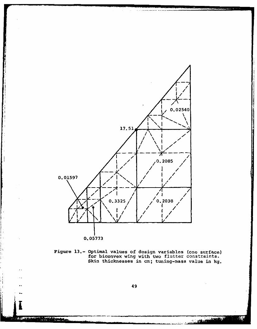
weight, less fuel, of 7,602 kg. The optimal skin thickness-~ distribution shown in figure 13 is quite different from that foundI L for multiple frequency constraints. Approximately 1.2 sec per

iteration were required by program SLACK for this problem.

6.5 Optimization with Flutter and Frequency Constraints

*A single flutter constraint (g <O at 262 m/sec) and a single

N frequency constraint (I > 6.20 Hz) were then imposed. After five

I iterations, a mode 4 crossover at a speed less than 262 m/sec was

again found. A flutter analysis of the fourth-iteration design

produced mode 2 and mode 4 crossovers similar to those in figure 11,

except that the mode 4 crossover was at 305 m/sec. Another flutter

S constraint was added - g <O at 305 m/sec - and an optimal solution

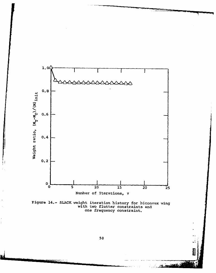
was found after 17 more iterations. The results for this problem

i are given in figures 14 and 15. The initial weight in figure 14

I 31

was that of the fourth-iteration design - 6,466 kg. The finalweight was virtually identical to that found with the flutter

constraints alone - 5,653 kg. This can also be seen in figure 15,where the optimal skin thickness distribution is very similar tothat given in figure 13. The previous parameter values were used

here in SLACK, and approximately 1.5 sec per iteration were

required.

7, CONCLUDING REMARKS

As noted in the discussion of the Gauss-Seidel iterativeprocedure for determining the Lagrange multipliers, the strategems

employed in program GAUSS are most effective when there are a

large number of constraints, so that determining the set ofconstraints that is active at the optimum is a genuine problem.In particular, this should be the case when stress constraints

are added to the behavioral constraints discussed in this report.Adding the capability to compute stresses and their derivativesis therefore a prime requirement in order to test program GAUSS

adequately.

The results from the optimization problems treated withprogram SLACK suggest that this program is reliable and easy to

use. Convergence properties, however, could be enhanced, probablyby a better selection of the various parameters that need to be

supplied by the user. More studies with variations of theseparameters would be useful. Also, it is time to treat largerproblems, and particularly to consider problems with stress

constraints, so that comparisons with program GAUSS can be

undertaken.

32

32

REFERENCES

1. McIntosh, S. C., Jr.: Modifications and Improvements in aStructural Optimization Scheme Based on an OptimalityCriterion. NEAR TR 169, June 1978.

2. Segenreich, S. A. and McIntosh, S. C., Jr.: Weight Minimi-

zation of Structures for Fixed Flutter Speed via an Opti-mality Criterion. AIAA Paper No. 75-779, presented at AIAA/ASME/SAE 16th Structures, Structural Dynamics, and MaterialsConference, Denver, CO, May 27-29, 1975.

3. Segenreich, S. A. and McIntosh, S. C., Jr.: Weight Optimiza-tion Under Multiple Equality Cbnstraints Using an OptimalityCriterion. Paper presented at AIAA/ASME/SAE 17th Structures,Structural Dynamics, and Materials Conference, King of Prussia,PA, May 5-7, 1976.

4. Segenreich, S. A., Zouain, N. A. and Herskovits, J.: An Opti-mality Criteria Method Based on Slack Variable Concept forLarge Scale Structural Optimization. Paper presented atSymposium on Application of Computer Methods in Engineering,University of Southern California, Los Angeles, CA, 1977.

5. Rizzi, P.: Optimization of Multi-Constrained StructuresBased on Optimality Criteria.. Proceedings AIAA/ASME/SAE

17th Structures, Structural Dynamics, and Materials Confer-ence, AIAA, New York, 1976, pp. 448-462.

6. Fleury, C. and Sander, G.: Structural Optimization by FiniteElement. Report NBR-SA-58, Jan. 1978, Aerospace Laboratory,University of Liege, Belgium.

7. Khot, N. S., Berke, L. and Venkayya, V. B.: Comparison ofOptimality Criteria Algorithms for Minimum Weight Design ofStructures. AIAA Journal, Vol. 16, No. 2, Feb. 1979,pp. 182-190.

8. Kiusalaas, J.: Minimum Weight Design of Structures viaOptimality Criteria. NASA TN D-7115, Dec. 1972.

9. Haftka, R. T. and Starnes, J. H., Jr.: WIDOWAC (Wing DesignOptimization with Aeroelastic Constraints): Program Manual.NASA TM X-3071, Oct. 1974.

10. Haftka, R. T. and Yates, E. C., Jr.: Repetitive Flutter Calcu-lations in Structural Design. Jour. Aircraft, Vol. 13, No. 7,July 1976, pp. 454-461.

33

REFERENCES (Concluded)

11. Craig, R. R., Jr. and Erbug, I. 0.: Application of aGradient-Projection Method to Minimum Weight Design of aDelta Wing with Static and Aeroelastic Constraints. Computersand Structures, Vol. 6, June 1976, pp. 529-538.

12. Khot, N. S., Berke. L. and Venkayya, V. B.: Minimum WeightDesign of Structures by the Optimality Criterion and ProjectionMethod. AIAA Paper No. 79-0720, presented at AIAA/ASME/ASCE/AHS 20th Structures, Structural Dynamics, and MaterialsConference, St. Louis, MO, April 4-6, 1979.

13. Gwin, L. B. and McIntosh, S. C., Jr.: A Method of Minimum-Weight Synthesis for Flutter Requirements, Part I - AnalyticalInvestigation. AFFDL TR 72-22, Part I, June 1972.

34I

34

0 01-4 cl OD Ln ON 0

0*

Ln

44 l r- m Nm H0 C% ( n %D~ H0 0

.,1) 0 0) H 0 0 0 0

0% am 0 -0. 0 NlIm co 0 co '0 %D 0

-1 N~ 0 m~ 1-0 0 0r0 0 oo0 0 0 0

44I I

> 0

dP 0 Ln Nl LA H-1~

4.44

0 4) N V%4.4 w A H 04-4 0J 0 H '0 H

6104- 4.)9 0 N '.0c Cl 0l-H 0 N r H OD C CD~ 01

4) C4 d IV 0* 0 0 C'L LA 044 ) U 0 0 *- N r- 0

4 -4 00 0 0 0 C4 0

04.

40 GO0m4 A) 01 Cl mA CD 0

-1,- Ln H- ( 0 H Ln 40

Q4 K %D 0 n 0 l H 1 -4 0to . l C! . .00 0 0 0 0 Cl

go4 5.4 LA Cl H - mA H f 0~

N. m I* in % I

'44 35

Table 2.- Variation of iterations requiredfor convergence with variousparameters in SLACK for testcase of figure 5.

€ K (V)v c max

0.001 0.5 2.'0 32

0.01 0.5 2.0 17

0.01 0.1 2.0 75

0,01 0.1 1.5 64

0.01 0.1 1.0 52

36

IIL* -

3.0

C ~0t1

t2

2 0-1020 t

~'igre .- lAC iteatin hstoy indesgn pac fo 2tes

377

3.0

t2 0

1.0

1.02.

Figure~~~~~~~~~~ 2.cLCotrtonhsoyi ein pc o -yst

case,~V" wih0 05 0 ~=09

38 001

1. 0 c2 4

3.0-

t2 c1 =0

/0

20-10 .

0 3

55 so

3.0-

t2C -0

2.0

0 1.0 2.0

Figure 4.- SLACK iteration history in design space for 2-Dy testcase, with~ 6 0 5, 6c 0.5, t= 0.9,

d =2.5$R 2. and =v 0.h01.

40

tC 0

3.01

2.0

.0 1.6.

Figure 5.'- SLACK iteration history in design space for 2-Dy testcase, with 6 -0 1 6C = 0.5, tl - 0.9v

d -2.5v 2:0: and e~ - 0.001.

41

t2

c3 0

1.4

1.2

1.0

0.8

0.4

0.2

00 0.2 0.4 0.6 0.8 1.0t

Figure 6.- GAUSS iteration history in design space for 2-Dy testcase, with a(O) - 0.5, a - 1.05, T~(0) - 0.35,

6x 1.05, ev 0.0, and e- 0.05. I42

50.5 deg.

3

10 2

2 1

14

Is 16 1325

I -fFigure5 13 pe-ufc oepit n oe-ae ubrn

21 19i9 24

( ) , ,-

,,/0

\/ I / ,

_j

-/ I A

/ l

I /I /

S I /

- / I N 1 /

\ I / I: /I 1/

Figure 8.- Design-variable linking for biconvex sandwich wing.

44

71

0

Ln

00

I

0 0' "4.

0 V

o ;

1400

454

I 0.02540

N.

17.51

/ \ I -

S \I,,

/ /tI / , /8 /I,, / /-- / I /

0.08184 ,'I K / 0.3627 /

- / I K /

/ ii1

/ ,, 0.2418 /0.02540 // /

/ 1

0. 1801

Figure 10.- Optimal values of design variables (one surface)for biconvex wing with two frequency constraints.Skin thicknesses in cm; tuning-mass value in kg.

46

....... .... .. I

0.3 I

0.2

Mode 2

0.1

H0-0.1 Md

U- -0.2

*-200 220 240 2602830

.1 V, rn/sec

Figure 11.- Critical V-g curves for biconvex wing withflutter constraint after 5th iteration

in SLACK.

i47

Ln

tp1

.1-IU

00

4JU

1-A

N44 $4

S >1 w

. 0

0) 4JO0 :%

0i

-'4IflkI

040

485

1,

do,0.054

9 g7

/ 0.208

0. 0597 0.05773I,

fo bicnve win g wihtofutrcntans

Figureki 3-O tinvales of cm d tsi niarias (one surface

49

1.0*

41 0.8

0.6

0.4

0.6

00 0 5202

Number 04Ieatos

Fiue1. LCKwih trtinhsoyfr iovxwn

Figure ~ ~ on 14-reqKueihti eration nstrainrt.ove wn

with two futrcntansa

_ 0.02540

17.51) \ I "

/\ I00/ \\J

/ /

/ /.1 / 02142 /

/ 7 I /0.02094 / ///

/ 0 .3 1 8 0 /

/- I / '/I /

- -- I //0.2206 /

, , / /II /., . -.,' I / /I /i/il' I\ \\1/ / I,/

0.03424

Figure 15.- Optimal values of design variables (one surface)for biconvex wing with two flutter constraintsand one frequency constraint. Skin thicknesses

in cm; tuning-mass value in kg.

51

"e- i__ ~-

NOMENCLATURE

ai Wright coefficient - see equation 0)

A Preliminary set of active or violated constraintsC

A Set of active or violated constraints as identifiedc by Gauss-Seidel iteration

i Av Set of active design variables

b Reference length

cc Inequality constraint function; jth inequalityconstraint function

2c! jth equality constraint function, c. +z.

C. Redesign factor on design variables

d Limiting value on la-lt - see equation (33)

D. Redesign factor on slack variables

E Young's modulus

EA Product of Young's modulus and cross-sectional area

[GA] Generalized aerodynamics matrix

[GM],[GK] Generalized mass and stiffness matrices, respectively

[GMi],[GK I] Derivatives of generalized mass and stiffness matriceswith respect to design variable ti

k Reduced frequency, wb/V.

K Step-size parameter for z.J

[Ki] Derivative of discrete stiffness matrix with respectto design variable t.

M Mass not available for optimization

MT Total mass

M Number of design variables

M. Mach number

52

ift0

NOMENCLATURE (Continued)

N Number of constraints

NA Number of active design variables

P£ Set of design variables predicted to reach a lowerbound during an iteration

P Set of all lower-bound passive variables

P Set of design variables predicted to reach an upper

U bound during an iteration

Pu Set of all upper-bound passive variables

t. ith design variable

u Displacment being constrained; rth displacement inr column of node-point displacements

tu,tx Parameters for determining Pu and Pt respectively

v. Convergence function - see equation (4)

v Normalized convergence function, v./ai

V. Free-stream speed

z. jth slack variable

a Step-size parameter

a Multiplier to determine a at each iteration -see equation (48)

jk Functions used in determining Lagrange multipliers -j'kj see equations (21) and (22)

kj Augmented function - see equation (25)

6t Step-size parameter used in determining la-li - seeequation (28)

Constraint-change parameter used in determiningIa-li - see equation (30)

Constraint tolerance parameter used to define A - seeequation (41)

53

NONMENCLATURE (Concluded)

6 Multiplier to determine T at each iteration seeX equation (49) c

EV Convergence parameter for v

C Convergence parameter for c

jth Lagrange multiplier

v Iteration number

V Poisson's ratio

p Mass density

' r Frequency; rth natural frequency

Eigenvalue from aeroelastic equations

( V Quantity at vth iteration

d )des Desired quantity

54 i

~II