249

ACREATING A MATHEMATICAL FLOOF AREA MODEL FOR NISTRU

RIVER, MARAMUREŞ COUNTY

Elemer-Emanuel SUBA1, Tudor SĂLĂGEAN1,2, Dumitru ONOSE1, Teodor RUSU2, Silvia CHIOREAN1, Florica MATEI2, Ioana POP2

1Technical University of Civil Engineering Bucharest, Lacul Tei 122-124, District 2,

020396, Bucharest, Romania 2University of Agricultural Sciences and Veterinary Medicine Cluj-Napoca,

3-5 Mănăştur Street, 400372, Cluj-Napoca, Romania

Corresponding author email: tudor.salagean@usamvcluj.ro Abstract This paper aims to determine the areas and the variations of hydrological and hydraulic modeling using modern software’s. As a case study for this paper I considered hydrologic and hydraulic modelling for Maramureş County for a watercourse, using HEC-RAS software. Although current software allows complex mathematical models, we should nevertheless consider the precision of imputed data, which most often affects the outcome. These errors must be identified and considered for a proper decision. It should be noted that no matter how well the work is executed, a hydro-technical project is not fully guaranteed, during its operation, due to major natural phenomenon that can degrade and cause hazards. Key words: flooding, hydraulic modeling, longitudinal profile, permanent flow mode, transversal profile. INTRODUCTION When asking "How much water is there?" we are beginning to talk about Hydrologic - Modelling (drain rainfall pattern). It aims to determine the water flow in the case of a storm in a known area. The main objective for hydrological modelling is finding the stream discharge, Q, in a certain location for a given rainfall event. This can be determined by statistical methods or by physical modelling. GIS is used to summarize the characteristics of the land and river basin models to integrate them into a pattern (Salagean et al., 2016). The main parameters to consider when working with hydrological modelling are: rainfall, evapotranspiration, terrain surface, water bodies, infiltration, groundwater, rivers and precipitation from a hydrographic pool (Maidment and Djokic, 2000). When wondering where water flows, we talk about hydraulic - modelling. Hydraulics allows us to see the amount of water flow and shape of the channel and determine how deep and fast

water will be, and what area (surface) it will cover in case of a flood. The main objective of hydraulic modelling is predicting growth of surface water in order to create flood risk maps. One can also predict water speed, quantity and quality of sediments (Maidment and Djokic, 2000; Burghila et al., 2016). As input data we need the geometry of the drainage canal and the hydraulic charac-teristics of the terrain, rainfall amount Q and surface, initial water level. As an output with hydrological modelling, we achieve surface and water depth within each section, along with other features. GIS is mainly used for assembling terrain charac-teristics (area determination), the integration and processing of hydraulic properties into a hydraulic model. MATERIALS AND METHODS To achieve hydraulic calculations for a river, the Hec GeoRas modul from ArcGis can be used, with the possibility of retrieving data directly in GIS from a digital elevation model

Janssen B.H. and Oenema O., 2008. Global economics of nutrient cycling. Turkish Journal of Agriculture and Forestry 32(3): p. 165-176.

Leip A., Britz W., Weiss F. & de Vries W., 2011. Farm, land, and soil nitrogen budgets for agriculture in Europe calculated with CAPRI. Environmental pollution, 159(11), p. 3243-3253.

Oenema O. et al., 2003. Approaches and uncertainties in nutrient budgets: implications for nutrient management and environmental policies. European Journal of Agronomy 20(1-2): p. 3-16.

Prăvălie R., Peptenatu D. and Sirodoev I., 2013. The impact of climate change on the dynamics of agricultural systems in south-western Romania. Carpathian Journal of Earth and Environmental Sciences 8.3: p. 175-186.

Spiess E., 2011. Nitrogen, phosphorus and potassium balances and cycles of Swiss agriculture from 1975 to 2008. Nutrient Cycling in Agroecosystems 91(3): p. 351-365.

***CHEMINOVA, 2017. Informații suplimentare. http://www.cheminova.ro/ro/produse/nutrienti/informatii_suplimentare/informatii_suplimentare.htm.

***GAMS General Algebraic Modelling System, 2013. www.gams.com.

***EUROSTAT, 2017. Agri-environmental indicator - gross nitrogen balance.

http://ec.europa.eu/eurostat/statistics.explained/index.php/Agri-environmental_indicator_-_gross_ nitrogen_ balance.

***INSSE Institutului national de statistica, 2017. Tempo Online. http://statistici.insse.ro/ shop/?lang=ro.

***OECD and EUROSTAT, 2007. Gross nitrogen balances – Handbook. http://www.oecd.org/ greengrowth/sustainableagriculture/40820234.pdf.

***Studiu comparativ intre technologia cultivarii graului in sistem conventional si tehnologia cultivarii graului in sistem egologic, 2017.

http://www.scritub.com/geografie/ecologie/studiu-comparativ-intre-tehnol92846.php.

***USDA Agricultural Research Service, 2017. USDA Food Composition, https://ndb.nal.usda.gov/ndb/ search/list?qlookup=10061.

AgroLife Scientific Journal - Volume 6, Number 1, 2017ISSN 2285-5718; ISSN CD-ROM 2285-5726; ISSN ONLINE 2286-0126; ISSN-L 2285-5718

250

or TIN but considering the lacking accuracy of patterns, they are represented by plotting the river system, banks, and identifying the central line of the bed and setting up a maximum extension study area, while also creating transverse profiles into sections we want to determining the desired water level for a certain flow (Bilasco and Csaba, 2016).

The survey was made with a South NTS665 total station, with a 5” angular accuracy. The integration of the survey into the national grid, Stereo 1970, was made using two south S82V dual frequency GPS receivers. The surveyed plan is shown in Figure 1.

Figure 1. Situation plan of the studied area

For obtaining this data we turned to a survey plan measured by us that served to design a bridge over the river Nistru from Tautii Magheraus, Maramures County. Based on surveying we determined seven cross sections which will be further processed with an open source version of HEC-RAS 5.0.1.

Main hydraulic variables such as water flow velocity and depth become constant over time (Figure 2) and a point in the stream. These parameters, which depend on the slope, roughness and geometry of the channel will be different, point after point along the river, depending on debit (Wang et al., 2017).

Figure 2. Schematic section of a stream, free surface and uniform flow Q, normal height yu and slope J (a); Schematic cross section of a stream with a moist section A and moist perimeter area P (b) (Marcou, 2010)

With annotations in Figure 2, the Manning-Strickler equation is written:

where: Q [m3/s] - is the flow; A [m2] - moist terrain surface; Kstr [m1/3/s] - velocity coefficient according to Strickler; RH [m] - hydraulic radius (RH=P/A, or P [m] moist perimeter). Building on the previous equation we can determine the motion (leak) according to the expression:

Kstr coefficient is proportional to the flow velocity and inversely proportional to the roughness of the terrain. Roughness is determined by the n coefficient, according to Manning. The relationship between Kstr and n becomes:

In order to form an opinion regarding the typical values for Kstr, we can see the next four examples (Figures 3 and 4).

Figure 3. Value for Kstr: a) Kstr = 45, watercourse arranged with concrete walls; b) Kstr = 42 broad watercourse, stony

251

or TIN but considering the lacking accuracy of patterns, they are represented by plotting the river system, banks, and identifying the central line of the bed and setting up a maximum extension study area, while also creating transverse profiles into sections we want to determining the desired water level for a certain flow (Bilasco and Csaba, 2016).

The survey was made with a South NTS665 total station, with a 5” angular accuracy. The integration of the survey into the national grid, Stereo 1970, was made using two south S82V dual frequency GPS receivers. The surveyed plan is shown in Figure 1.

Figure 1. Situation plan of the studied area

For obtaining this data we turned to a survey plan measured by us that served to design a bridge over the river Nistru from Tautii Magheraus, Maramures County. Based on surveying we determined seven cross sections which will be further processed with an open source version of HEC-RAS 5.0.1.

Main hydraulic variables such as water flow velocity and depth become constant over time (Figure 2) and a point in the stream. These parameters, which depend on the slope, roughness and geometry of the channel will be different, point after point along the river, depending on debit (Wang et al., 2017).

Figure 2. Schematic section of a stream, free surface and uniform flow Q, normal height yu and slope J (a); Schematic cross section of a stream with a moist section A and moist perimeter area P (b) (Marcou, 2010)

With annotations in Figure 2, the Manning-Strickler equation is written:

where: Q [m3/s] - is the flow; A [m2] - moist terrain surface; Kstr [m1/3/s] - velocity coefficient according to Strickler; RH [m] - hydraulic radius (RH=P/A, or P [m] moist perimeter). Building on the previous equation we can determine the motion (leak) according to the expression:

Kstr coefficient is proportional to the flow velocity and inversely proportional to the roughness of the terrain. Roughness is determined by the n coefficient, according to Manning. The relationship between Kstr and n becomes:

In order to form an opinion regarding the typical values for Kstr, we can see the next four examples (Figures 3 and 4).

Figure 3. Value for Kstr: a) Kstr = 45, watercourse arranged with concrete walls; b) Kstr = 42 broad watercourse, stony

252

Figure 4. Value for Kstr: a) Kstr = 31 soft watercourse on alluvial bed; b) Kstr = 20 natural watercourse

with side vegetation and mobile alluvial bed

For hydraulic calculus a weighted average for Kstr is determined. Etching the vertical direction must be carried out so as to obtain a constant roughness within each of the etched parts. RESULTS AND DISCUSSIONS The need for rapid calculation of water level profiles (given the rapid manifestation of extreme hydrological conditions) and the astonding developmentof modern computing have contributed to the possibility of implementing equations within the software to run on diverse operating systems (Bilasco and Csaba, 2016).

Work steps for hydraulic modeling for the river Nistru, Tautii Magheraus, Maramureş County:

• Surveying; • Creating transverse profiles and profile

data entry to Microsoft Excel for ease of use in HEC-RAS;

• Creation of the HEC-RAS project; • Data Import • Adding Manning coefficients for each

section; • Hydrological model; • Model calculus.

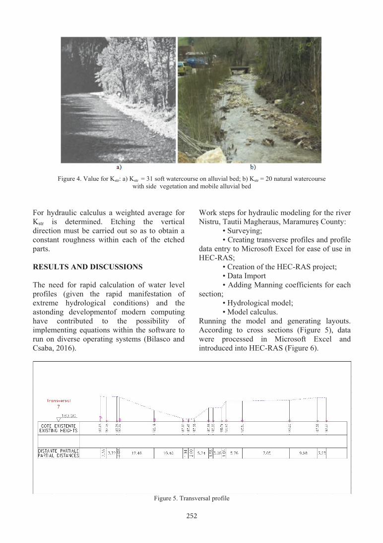
Running the model and generating layouts. According to cross sections (Figure 5), data were processed in Microsoft Excel and introduced into HEC-RAS (Figure 6).

Figure 5. Transversal profile

Figure 6. Transversal profile HEC-RAS

In a similar manner we imported the geometries for each cross section profile, from 1 to 7 and subsequently we specified the distances between them, based on the longitudinal profile axis. Introducing cross sections is made from upstream to downstream. Depending on the natural conditions we see on the field, we will choose the value of Manning coefficients from the table provided by Bilasco and Csaba (2016) and we will associate every

section part for transversal profiles. On a longitudinal plan, between two cross sections, the software will make an average between set coefficients. In Figure 7 we can see the main features for Nistru river bank. Based on these characteristics we selected and introduced Manning coefficients using the graphical editor XS, for the left bank, right bank and the flow zone (Figure 8).

Figure 7. Nistru river bank - Tautii Magheraus, Maramureş County

253

Figure 4. Value for Kstr: a) Kstr = 31 soft watercourse on alluvial bed; b) Kstr = 20 natural watercourse

with side vegetation and mobile alluvial bed

For hydraulic calculus a weighted average for Kstr is determined. Etching the vertical direction must be carried out so as to obtain a constant roughness within each of the etched parts. RESULTS AND DISCUSSIONS The need for rapid calculation of water level profiles (given the rapid manifestation of extreme hydrological conditions) and the astonding developmentof modern computing have contributed to the possibility of implementing equations within the software to run on diverse operating systems (Bilasco and Csaba, 2016).

Work steps for hydraulic modeling for the river Nistru, Tautii Magheraus, Maramureş County:

• Surveying; • Creating transverse profiles and profile

data entry to Microsoft Excel for ease of use in HEC-RAS;

• Creation of the HEC-RAS project; • Data Import • Adding Manning coefficients for each

section; • Hydrological model; • Model calculus.

Running the model and generating layouts. According to cross sections (Figure 5), data were processed in Microsoft Excel and introduced into HEC-RAS (Figure 6).

Figure 5. Transversal profile

Figure 6. Transversal profile HEC-RAS

In a similar manner we imported the geometries for each cross section profile, from 1 to 7 and subsequently we specified the distances between them, based on the longitudinal profile axis. Introducing cross sections is made from upstream to downstream. Depending on the natural conditions we see on the field, we will choose the value of Manning coefficients from the table provided by Bilasco and Csaba (2016) and we will associate every

section part for transversal profiles. On a longitudinal plan, between two cross sections, the software will make an average between set coefficients. In Figure 7 we can see the main features for Nistru river bank. Based on these characteristics we selected and introduced Manning coefficients using the graphical editor XS, for the left bank, right bank and the flow zone (Figure 8).

Figure 7. Nistru river bank - Tautii Magheraus, Maramureş County

254

Figure 8. Determining the Maning coefficients by the transversal profiles

The distances between the transverse profiles were introduced in HEC-RAS. From the editing menu, with help from a specific window, the user can access information regarding profile height, its length, information found on the two axis and information regarding the Manning coefficient values for the three sections. For running the Hydraulic model, data is necessary regarding flow, debit, upstream and downstream riverbed slope regarding section profile calculation. The integration of these data in the HEC-RAS project is done using the module Steady Flow Data, if the flow is considered uniform. Another factor shaping the outflow, and that is taken into account in the hydraulic modeling of the water level profile, is the bed slope (Beilicci, 2016). Steady Flow Data Module allows data introduction regarding slope value/characteristics for downstream and upstream for profile calculated

used to calculate the water level profile, based on the Manning equation. Entering data regarding debit, as multiple values for each separate profile is achieved in part using the submenu reach Boundary Conditions. Having completed calculations, HEC-RAS has a graphical and numerical interface, for viewing the final result. It can be viewed the water level determined for each profile in part and a summary of the results, as numerical values calculated from equations defining the model for each profile/part. For cross sections the table and cross section output is presented in Figure 9 and the graphics (cross section) in Figure 10. Water level for the profile can be distinguished, according to Q moment - minimum and T = 100 - maximum. Also data on hydraulic model profile can be viewed in a table, accessing summary output table by profile (Figure 11).

Figure 9. Cross section output

Figure 10. Cross section graphical output

Figure 11. Longitudinal profile table output

255

Figure 8. Determining the Maning coefficients by the transversal profiles

The distances between the transverse profiles were introduced in HEC-RAS. From the editing menu, with help from a specific window, the user can access information regarding profile height, its length, information found on the two axis and information regarding the Manning coefficient values for the three sections. For running the Hydraulic model, data is necessary regarding flow, debit, upstream and downstream riverbed slope regarding section profile calculation. The integration of these data in the HEC-RAS project is done using the module Steady Flow Data, if the flow is considered uniform. Another factor shaping the outflow, and that is taken into account in the hydraulic modeling of the water level profile, is the bed slope (Beilicci, 2016). Steady Flow Data Module allows data introduction regarding slope value/characteristics for downstream and upstream for profile calculated

used to calculate the water level profile, based on the Manning equation. Entering data regarding debit, as multiple values for each separate profile is achieved in part using the submenu reach Boundary Conditions. Having completed calculations, HEC-RAS has a graphical and numerical interface, for viewing the final result. It can be viewed the water level determined for each profile in part and a summary of the results, as numerical values calculated from equations defining the model for each profile/part. For cross sections the table and cross section output is presented in Figure 9 and the graphics (cross section) in Figure 10. Water level for the profile can be distinguished, according to Q moment - minimum and T = 100 - maximum. Also data on hydraulic model profile can be viewed in a table, accessing summary output table by profile (Figure 11).

Figure 9. Cross section output

Figure 10. Cross section graphical output

Figure 11. Longitudinal profile table output

256

CONCLUSIONS Surveying work carried out on Nistru river, Tautii Magheraus, Maramureş County, served for the design and implementation of a new bridge over the creek, considering the degree of degradation of the existing wood bridge. In regards to the design and execution of the bridge, it was carried out by a specialized company, which was completed in early 2016. The minimum height of the lower metal deck of the bridge was designed and built at an absolute height of 187.8 m (Black Sea, 1970). The bridge is slightly arched in the middle so we took into consideration the lowest height of the abutment. The bridge was placed between the 4th and 5th transversal profile (Figure 12) near the old bridge’s location, which was eventually decommissioned.

Figure 12. Bridge across Nistru River

Analyzing hydraulic modelling results obtained with HEC RAS, presented above, regarding the location and the inferior height of the new bridge deck, we can see that it was designed over the critical hydraulic height, profile 5 – has a maximum critical height of 187.51 m and profile 4 - 186.07 m. An approximate average for water critical height would be 186.8 m. Considering that the bridges lower deck height is 187.8 m, it has 1m above the critical threshold. Of course nature forces have no limitations and should not be excluded any possible variant of

flooding but in terms of hydraulic modelling, the location of this bridge is correct. Hydraulic modelling using HEC-RAS software for the databases riverbed geometry representation and water flow speed, is a fast and useful method if the accuracy of entry database is high enough and we have sufficient information about the elements that influence the water flow and debit. The accuracy of the final results depend 100% on the accuracy of the elements introduced into the modelling process. ACKNOWLEDGEMENTS This work was performed under the frame of the Partnership in priority domains - PNII, developed with the support of MEN-UEFISCDI, project no. PN-II-PT-PCCA-2013-4-0015: Expert system for monitoring risks in agriculture and agricultural technologies conservative adaptation to climate change. REFERENCES Beilicci R., Beilicci E., 2016. Advance hydraulic

modeling of Mehadica river, Romania, Caras Severin county. Scientific Bulletin of the Politehnica University of Timişoara, Romania, Volume 61 (75), Issue 2.

Bilasco S., Csaba H., 2016. Digital mapping of bands flooding based on statistics, hydraulic calculations and GIS spatial analysis. Casa Cartii de Stiinta Publishing House, Cluj-Napoca, Romania.

Burghila C., Bordun C., Cimpeanu S.M., Burghila D., Badea A., 2016. Why mapping ecosystems services is a must in EU biodiversity strategy for 2020? AgroLife Scientific Journal, Vol. 5(2), p. 28-37.

Maidment D.R., Djokic D., 2000. Hydrologic and Hydraulic Modelling Support: With Geographic Information Systems. Esri Press, USA.

Marcou O., 2010. Modelisation et controle d’ecoulements a surface libre par la methode de Boltzmann sur reseau. These de doctorat, Geneve University, no. Sc. 4214.

Salagean T., Rusu T., Porutiu A., Deak J., Manea R., Virsta A., Calin M., 2016. Aspects regarding the achieving of a geographic information system specific for real estate domain. AgroLife Scientific Journal, Vol. 5 (2), p. 137-142.

Wang J., 2017. Simulating the hydrologic cycle in coal mining subsidence areas with a distributed hydrologic model. Sci. Rep. 7.

 CLINICAL AND PARACLINICAL PECULIARITIES

OF EFFUSIVE FELINE INFECTIOUS PERITONITIS UNDER NON-SPECIFIC IGY TREATMENT: CASE STUDY

Teodora Diana SUPEANU1, Alexandru SUPEANU2, Dragoş COBZARIU1,

Stelian BĂRĂITĂREANU1, Doina DANEŞ1

¹University of Agronomic Sciences and Veterinary Medicine of Bucharest, Faculty of Veterinary Medicine, 105 Splaiul Independenţei, RO 050097, Bucharest, Romania

²Romanian Academy, 125 Victoriei Road, RO 010071, Bucharest, Romania

Corresponding author email: supeanu.teodora@gmail.com Abstract Feline infectious peritonitisis a disease determined by a coronavirus, affectingdomestic and wild cats and once triggered is fatal in almost 100%. The occurrence of the related pathology are yet to be fully determined; currently, a certain and confident in-clinicaldiagnosis is unavailable, as is the case for an efficient vaccine or a treatment that will restore to health. These make the feline infectious peritonitis a subject currently undergoing intensive research studies. The paper presents the case of a 5 months cat patient manifesting the rapid evolution effusive form of the disease. The aim of study was to evaluate if the variation of the 24 biological parameters studied was significant under treatment with immunoglobulins of avian origin. The patient tolerated well the supportive therapy based on egg yolk Immunoglobulin Y, without evidences of side effects. Key words: feline infectious peritonitis, immunoglobulin Y, immunomodulatory treatment. INTRODUCTION Feline infectious peritonitis (FIP) is a severe multi-systemic immune-enhanced disease of cats, progressive and always deadly, associated with feline coronavirus (FCoV) (Brown et al., 2009; Cobzariu et al., 2015); also, it is a major factor in kitten mortality (Hartmann, 2005). In current Romanian practice, the difficulty of FIP confirmation caused under-diagnosis of disease in several cases (Cobzariu et al., 2015). Despite the weakness of the detection, Feline Enteric Coronavirus (FECV) is prevalent mainly in high-density environments, with limited clinical consequence (Kim et al., 2016). FCoVs have two pathotypes: the feline enteric coronavirus (FECV) and the feline infectious peritonitis virus (FIPV). The two pathotypes recognize different primary replication site, this feature being related with the clinical outcome. It is accepted the theory that FIPV is originating from FECV infected cats by genetic alterations - gaining tropism for macrophages - and inducing the FIP disease (Bálintet et al., 2012; Tanaka et al., 2012; Kim et al., 2016).

FCoV diagnosis based on antibody titration, antigen detection or PCR-based tests can’t differentiate the strains. Actually, histopa-thology and immuno-histochemistry are the reliable confirmatory procedure but laborious for in-clinical diagnosis (Cobzariu et al., 2015). Until present is neither effective treatment, vaccine, nor diagnostic protocol able to discriminate the FECV from FIPV (Brown et al., 2009). However, a small ratio of cats develops FIP during the FECV infection. Reliable studies support the important role of immune system in the pathogenesis of FIP. OPTIONS OF TREATMENT FOR FIP Many strategies have been developed to cure FIP. Interferons inhibit the FIPV in vitro but not in vivo. Various immunosuppressants have been studied, but although these drugs increase life average, the FIPV infection remains fatal. Therefore, an effective vaccine and a therapeutic medicine to FIPV are still looking for (Tanaka et al., 2012). The immunoglobulin Y (IgY) is present in birds and mainly in the egg-yolk (Bentes et al., 2015). The IgY is playing the functional role of