GEOPHYSICS. VOL. 49, NO. 5 (MAY 1984); P. 533-549, 13 FIGS.

Accuracy of finite-difference and finite-element modeling of the scalar and elastic wave equations

Kurt J. Marfurt*

ABSTRACT

Numerical solutions of the scalar and elastic wave equations have greatly aided geophysicists in both for- ward modeling and migration of seismic wave fields in complicated geologic media, and they promise to be invaluable in solving the full inverse problem. This paper quantitatively compares finite-difference and finite-element solutions of the scalar and elastic hyper- bolic wave equations for the most popular implicit and explicit time-domain and frequency-domain techniques.

In addition to versatility and ease of implementation, it is imperative that one choose the most cost effective solution technique for a fixed degree of accuracy. To be of value, a solution technique must be able to minimize (1) numerical attenuation or amplification, (2) polariza- tion errors, (3) numerical anisotropy, (4) errors in phase and group velocities, (5) extraneous numerical (parasitic) modes, (6) numerical diffraction and scattering, and (7) errors in reflection and transmission coefficients.

This paper shows that in homogeneous media the explicit finite-element and finite-difference schemes are comparable when solving the scalar wave equation and when solving the elastic wave equations with Poisson’s ratio less than 0.3. Finite-elements are superior to finite- differences when modeling elastic media with Poisson’s ratio between 0.3 and 0.45. For both the scalar and elastic equations, the more costly implicit time integra- tion schemes such as the Newmark scheme are inferior to the explicit central-differences scheme, since timesteps surpassing the Courant condition yield stable but highly inaccurate results. Frequency-domain finite- element solutions employing a weighted average of con- sistent and lumped masses yield the most accurate re- sults, and they promise to be the most cost-effective method for CDP, well log, and interactive modeling.

INTRODUCTION

Numerically modeling wave fields via finite-difference, finite- element, or boundary integral equation techniques has already established itself as a valuable tool in forward modeling and

migration, and it holds great promise for the solution of the full inverse problem (simultaneous migration and parameter inver- sion). However, the large-scale implementation of these tech- niques has outpaced a quantitative analysis of their accuracy. What little is known of these accuracies is widely scattered in the literature. Alford et al (1974) analyzed the accuracy of second- and fourth-order finite-difference solutions of the two- dimensional (2-D) scalar wave equation using central differ- ences in time Belytichko and Mullen (1978) analyzed the accu- racy of second- and fourth-order finite-element solutions of the 2-D scalar wave equation in the frequency domain. Quite re- cently, Bamberger et al (1980) carefully analyzed the accuracy and stability ofsecond-order finite-difference and finite-element solutions of the elastic wave equations using central differences in time

The discretization of a continuum as achieved by finite- difference, finite-element, or boundary integral equation tech- niques yields progressively more accurate solutions as the mesh size becomes finer. In this regard, numerical modeling may be considered to be a low-pass filter, in the sense that low fre- quencies (wavelengths that are long when compared with the grid spacing) accurately propagate through the mesh, whereas high frequencies (short wavelengths) are undesirably modified, undergoing (1) numerical attenuation or amplification (includ- ing numerical amplication of roundoff errors), (2) numerical anisotropy where propagation velocities vary with orientation to the discretization mesh, (3) numerical phase and group ve- locity dispersion where velocity is now a function of mesh points per wavelength, and (4) numerical polarization where longitudinally or transversely polarized wave fields become quasi-longitudinal and quasi-shear wave fields. In addition, higher order schemes (Belytichko and Mullen, 1978) and inho- mogeneous meshes (Mullen and Belytichko, 1980) will generate parasitic (pureiy numericai) modes of vibration, particuiariy at higher frequencies, that must be suppressed.

THE WEIGHTED RESIDUAL METHOD

Spatial discretization

Numerical techniques such as finite-differences, finite- elements, boundary integral equations, and the method of mo- ments all belong to the more general weighted residual method

Manuscript received by the Editor May 20, 1982; revised manuscript received October 14, 1983. *Amoco Production Company, P. 0. Box 591, Tulsa, OK 74102. \(a, 1984 Society of Exploration Geophysicists. All rights reserved.

Dow

nloa

ded

01/0

7/21

to 2

07.1

95.5

3.8.

Red

istr

ibut

ion

subj

ect t

o S

EG

lice

nse

or c

opyr

ight

; see

Ter

ms

of U

se a

t http

s://l

ibra

ry.s

eg.o

rg/p

age/

polic

ies/

term

sD

OI:1

0.11

90/1

.144

1689

534

(Brebbia, 1978; Pinder and Gray, 1977; Zienkiewicz, 1977). Given a linear differential equation

L(u,) - q = 0 in domain R,

subject to essential boundary conditions,

A@,) = 91 on surface Ii

and natural boundary conditions

B(u,) = 92 on surface F2,

one may approximate the exact solution u,, by

u= 2aK+K, K=l

where $k are linearly independent basis functions (called shape functions or interpolation functions in finite-element analysis). In finite-element and finite-difference analyses, the coefficients a, take on the value of the field u at a discrete number of nodal points. The error E of this approximation at a given point may be expressed as

& = L(u) - q = L [ 1 ; aK4k -q#o. K=l

The weighted residual method requires that the weighted average of this error, or residual, go to zero in the domain R:

s EWJ dR = 0, J = 1, 2, . . , N,

where wJ are arbitrary weighting functions. Forcing E to be zero at a discrete number of points

WJ = T &*.I 6(x, > t,)

generates all possible finite-difference solutions, where BrkJ are constant weights.

Choosing i+rJ = +J such that the weighting and basis func- tions are identical generates the Galerkin formulation of the finite-element method,

jqldl-l=jEc$Idi-12

J = 1, 2, , N,

giving a linear system of equations in aK,

;,uk 5 L(+rJ+J dD =

s q+J dQ J = 1, 2, . . , N. (1)

Exploration seismologists are interested in modeling the fol- lowing important 2-D problems. The generalization to three- dimensions is theoretically simple, though computationally more expensive.

(1) Acoustics

L(P) - q = v * (;vP)-.g~.g)-q=O, where

Marturt

P = pressure, p = density, )i = Lame’s parameter (or bulk modulus, since u = 0),

and q = source.

(2) Antiplane strain (SH waves)

_/ Yu,) - q = v * (pVu,) - ; ( > p 2 - qy = 0,

where

u, = horizontal, out-of-plane component of displacement, u = Lame’s parameter (shear modulus),

and qy = horizontal, out-of-plane component of the source.

(3) Plane strain elasticity

L(u) - q = V[(k + j.l)V * u] + v * (pVu) - & ( >

p ; - q = 0,

where

u = (u,, uz) are the in-plane components of displacement, and

q = (q,, q,) are the in-plane components of the source.

For 2-D acoustics, letting

N P = C uK&,

K=l

equation (1) becomes

Integrating the left-hand side by parts and assuming 1 does not vary with time one obtains

where 6 denotes the normal to the surface F enclosing the volume R. Equation (2) is considered to be a “weak form” of the acoustic wave equation since l/p no longer need be differ- entiable as it was in equation (1) (wJ must now be first-order differentiable).

Assuming homogeneous Neumann boundary conditions, such that the integral over F vanishes, or assuming the integral over I cancels on assemblage of adjacent elements, equation (2) may be written succinctly as

$

N m,,ii,+ 1 k,,u,+f,=O, J = 1, 2, ., N, (3)

K=l K=l

where the elemental “mass,” “ stiffness,” and “load” matrices are given by

Dow

nloa

ded

01/0

7/21

to 2

07.1

95.5

3.8.

Red

istr

ibut

ion

subj

ect t

o S

EG

lice

nse

or c

opyr

ight

; see

Ter

ms

of U

se a

t http

s://l

ibra

ry.s

eg.o

rg/p

age/

polic

ies/

term

sD

OI:1

0.11

90/1

.144

1689

Modeling of Elastic Wave Equations 535

l---f+ A( 4

~-

I/-

III_

Y

-+

i

3 7

1. 1 2 6 area collocation

I 2

1 1 2 7 Newmark

forward differences

0 centra 1 differences

1 backward differences

1. 10 linear acceleration

Galerkin

Fox-Goodwin

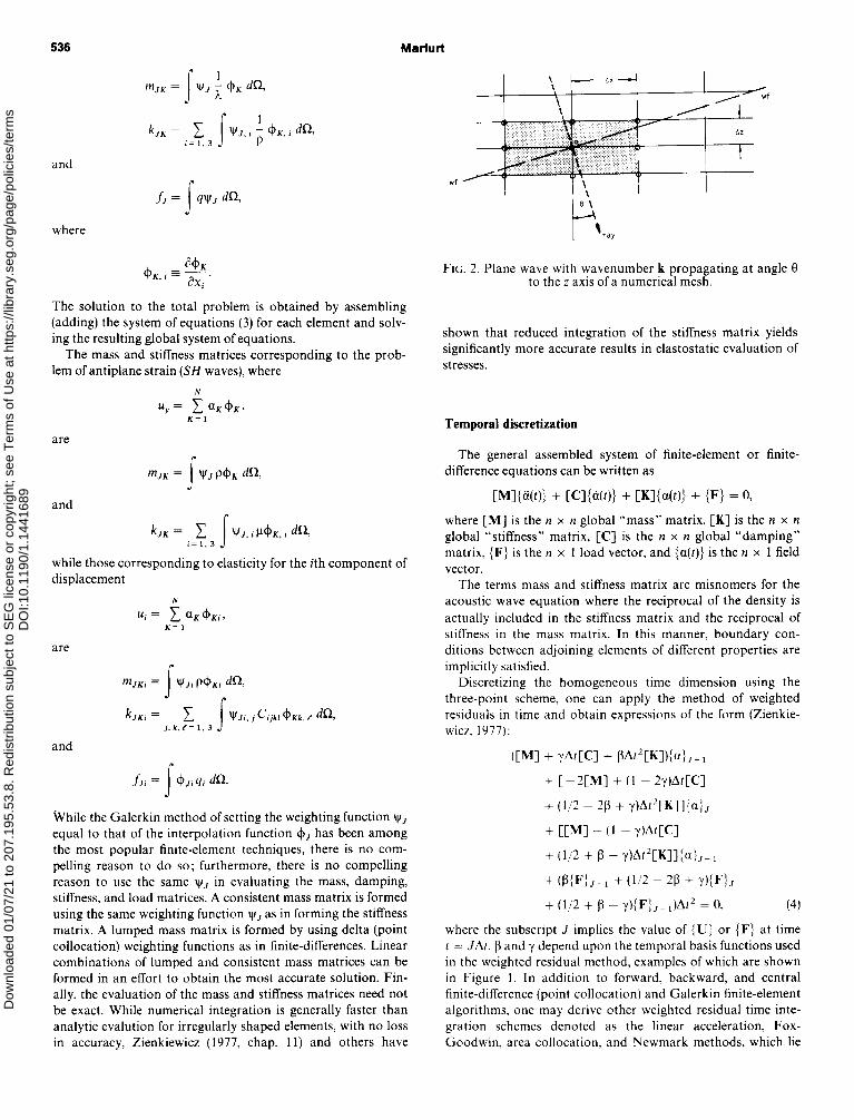
FIG. 1. Interpolation functions 4(t) and weighting function w(t) used in three-level time integration schemes. y and p are those used in equation (4) (after Zienkiewicz, 1977, p. 583).

Dow

nloa

ded

01/0

7/21

to 2

07.1

95.5

3.8.

Red

istr

ibut

ion

subj

ect t

o S

EG

lice

nse

or c

opyr

ight

; see

Ter

ms

of U

se a

t http

s://l

ibra

ry.s

eg.o

rg/p

age/

polic

ies/

term

sD

OI:1

0.11

90/1

.144

1689

Maffurt

and

where

The solution to the total problem is obtained by assembling (adding) the system of equations (3) for each element and solv- ing the resulting global system of equations.

The mass and stiffness matrices corresponding to the prob- lem of antiplane strain (SH waves), where

N

uy= C a,+,, K=1

are

and

k,, = C s WJ. i P$K. i dQ i=1,3

while those corresponding to elasticity for the ith component of displacement

N

ui= 1 aft+Kir

K=l

are

m JKi = VJi P+K~ dQ

and

fJi = +Jiqi da. s While the Galerkin method of setting the weighting function wJ equal to that of the interpolation function $J has been among the most popular finite-element techniques, there is no com- pelling reason to do so; furthermore, there is no compelling reason to use the same wJ in evaluating the mass, damping, stiffness, and load matrices. A consistent mass matrix is formed using the same weighting function I+I~ as in forming the stiffness matrix. A lumped mass matrix is formed by using delta (point collocation) weighting functions as in finite-differences. Linear combinations of lumped and consistent mass matrices can be formed in an effort to obtain the most accurate solution. Fin- ally, the evaluation of the mass and stiffness matrices need not be exact. While numerical integration is generally faster than analytic evalution for irregularly shaped elements, with no loss in accuracy, Zienkiewicz (1977, chap. 11) and others have

FE. 2. Plane wave with wavenumber k propagating at angle 8 to the z axis of a numerical mesh.

shown that reduced integration of the stiffness matrix yields significantly more accurate results in elastostatic evaluation of stresses.

Temporal discretization

The general assembled system of finite-element or finite- difference equations can be written as

CMl{W) + CWW + CKl{W) + IF) = 0,

where [M] is the n x n global “mass” matrix, [K] is the n x n

global “stiffness” matrix, [C] is the n x n global “damping” matrix, {FJ is the n x 1 load vector, and {a(t)} is the n x 1 field vector.

The terms mass and stiffness matrix are misnomers for the acoustic wave equation where the reciprocal of the density is actually included in the stiffness matrix and the reciprocal of stiffness in the mass matrix. In this manner, boundary con- ditions between adjoining elements of different properties are implicitly satisfied.

Discretizing the homogeneous time dimension using the three-point scheme, one can apply the method of weighted residuals in time and obtain expressions of the form (Zienkie- wicz, 1977):

WI + yAtCC1 + @f’[Kl){aiJ+ I

+ [-2[M] + (1 - 2y)At[C]

+ (l/2 - 2p + Y)Af2[K]]{a)J

+ CPU - (1 - YMCI

+ (112 + b - y)At2[Kll{a),m,

+ (B(F),+ 1 + (11’2 - 2P + Y)IF)J

+ (1,/2 + )3 - y){F),_,)At2 = 0, (4)

where the subscript J implies the value of {U) or {F} at timet = JAt. f3 and y depend upon the temporal basis functions used in the weighted residual method, examples of which are shown in Figure 1. In addition to forward, backward, and central finite-difference (point collocation) and Galerkin finite-element algorithms, one may derive other weighted residual time inte- gration schemes denoted as the linear acceleration, Fox- Goodwin, area collocation, and Newmark methods, which lie

Dow

nloa

ded

01/0

7/21

to 2

07.1

95.5

3.8.

Red

istr

ibut

ion

subj

ect t

o S

EG

lice

nse

or c

opyr

ight

; see

Ter

ms

of U

se a

t http

s://l

ibra

ry.s

eg.o

rg/p

age/

polic

ies/

term

sD

OI:1

0.11

90/1

.144

1689

Modeling of Elastic Wave Equations 537

in the gray area between finite-elements and finite-differences (Bathe and Wilson, 1976, p. 350; Zienkiewicz, 1977, p. 581).

As an alternative to three-point and higher order temporal schemes, one may wish to effect a Fourier transform of the load vector {F(t)) into the temporal frequency (0) domain and obtain the Fourier components {c(o)} of {u(t)} :

(-d[M] + iw[C] + [K])‘,&(o)j + {i$)j = 0

by simple Gaussian elimination at each frequency. {a(t)) may then be obtained by an equally fast inverse Fourier transform.

ACCURACY IN NUMERICALLY MODELING THE SCALAR WAVE EQUATION

Principles

In an infinite homogeneous, isotropic medium with no damping, the 2-D acoustic and antiplane strain (SH wave) equations may be written in the following form:

where ci = h/p for acoustic waves, and ci = p/p for SH waves. For a homogeneous, isotropic medium, both the phase and group velocities of wave propagation are constant and equal to cO. Numerically modeling a continuous isotropic medium by, at best, piece-wise continuous interpolation or shape functions +J will generate both numerically dispersive and anisotropic solutions. To evaluate these errors quantitatively, consider a displacement field imposed upon the mesh of the form

U(-uK , -7K 1 f.r) E a,@,)

=4(x,, 2~) exp {i[k,x, + k,z, - ~t,l>,

where k, = k sin 8, and kz = k cos 8, and where 8 is the angle between the ray normal to the plane wave and the z-axis (Figure?); For a homogeneous, isotropic continuum, the tem- poral frequency is given by o(k) = kc,, where cc, is defined in equation (5). The phase velocity cph and group velocity cgr are

w(k) kc, c,,=k=-=CO’

k

and

do(k) 3 c 81 = - = k (kc,) = co.

dk

For a numerical solution, o(k) may be obtained by finding the roots of the determinant of the n x n system of equations (4).

+ C-2MIK + UP - 2P + W2&KlaK, J

+ CM,, + UP + P - y)At 2 GJa,, J-1 = 0 9

I = 1, 2, . . , n. (f-9

Finding the roots of such an n x n system of equations can be extremely difficult, and impossible as n+ ~13. However, for a homogeneous mesh with constant Ax and AZ in a homoge-

Finite Differences Finite Elements

t;t SCALAR

I I I I

ELASTIC Horizontal dgf

Vertical dgf

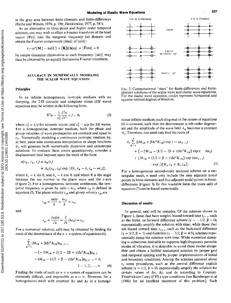
FIG. 3. Computational “stars” for finite-differences and finite- element solutions of the scalar wave and elastic wave equations. For the elastic wave equation, circles represent horizontal and squares vertical degrees of freedom.

neous infinite medium, each diagonal of the system of equations (6) is constant, such that the determinant is &h-order degener- ate and the amplitude of the wave field A, becomes a constant A,. Therefore, one need only find the roots of

A,K$lI(M,~ + BAr2K,,) exp ( - w,+ A

+ [-2M,, + (l/2 - 28 + y)Af’K,,] exp ( - iot,)

+ [Ml, + (l/2 + B - y)At’K,,] exp (iwt,_ ,)

exp {i[K,x, + K,z,l}. (7)

For a homogeneous second-order accurate scheme on a rec- tangular mesh, n need only include the nine adjacent nodal points in finite-elements and five adjacent nodal points in finite- difference (Figure 3). in this tractable- form then roots o(k) of equation (7) can be found numerically.

Discussion of results

In general, o(k) will be complex. Of the schemes shown in Figure 1, those that have weights biased toward time t,_ i, such as the Euler, or forward difference scheme (y = -l/2, B = 0), exponentially amplify the solution with time while those that are biased toward time tJ+i, such as the backward difference (y = 3/2, B = 1) and Galerkin (y = 3/2, B = 4/5), schemes expo- nentially damp the solution with time While numerical damp- ing is sometimes desirable to suppress high-frequency parasitic modes of vibration, it is desirable to avoid these modes altoge- ther and obtain a faithful undamped solution by proper grid and temporal spacing and by proper implementation of initial and boundary conditions. Among the schemes centered about t, some procedures, such as the central difference explicit scheme (y = l/2, B = 0), exponentially amplify the solution for certain values of Ax, AZ, and At according to Courant- Friedrickson-Lewy (CFL) type conditions [see Bamberger et al (1980) for an excellent treatment of this problem]. Such

Dow

nloa

ded

01/0

7/21

to 2

07.1

95.5

3.8.

Red

istr

ibut

ion

subj

ect t

o S

EG

lice

nse

or c

opyr

ight

; see

Ter

ms

of U

se a

t http

s://l

ibra

ry.s

eg.o

rg/p

age/

polic

ies/

term

sD

OI:1

0.11

90/1

.144

1689

538 Marturl

(cl

P h,

6

Fw. 4. Dispersion curves for finite-element solution of the scalar wave equation. Phase velocity C,, and group velocity Cc, along the z axis (0 = 0 degrees) are normalized with respect to the true velocity C, and plotted versus wavenumber k* = kAx/2rt = Ax/h = l/G where G is the number of grid points per wavelength. p = C,At/Ax is the normalized time step. (a) Explicit finite-differences in time using a lumped mass matrix. (b) Implicit Newmark method in time using a lumped mass matrix. (c) Implicit Newmark method in time using a consistent mass matrix. In all three cases, the frequency-domain solution corresponds to the curve p = 0. p = 1.0 is the Courant stability limit.

Dow

nloa

ded

01/0

7/21

to 2

07.1

95.5

3.8.

Red

istr

ibut

ion

subj

ect t

o S

EG

lice

nse

or c

opyr

ight

; see

Ter

ms

of U

se a

t http

s://l

ibra

ry.s

eg.o

rg/p

age/

polic

ies/

term

sD

OI:1

0.11

90/1

.144

1689

Modeling of Elastic Wave Equations

cGR'c~

(A)

l.lO;-

1.05 ;-

(B) ;

1.00;

__________._....._...--..--._

(cl i

1.00 w ___.

0.95; . . .._ _.__

IO

50

I00 150

1.10

1.05

1.00

0.95

0.90

_.......... 3 O0 150

1.05

1.00

0.95

0.90 ‘;--‘; \ ._ _..1....... ‘..30!

1.05

1.00

0.95

0.90

us0

300

00

150

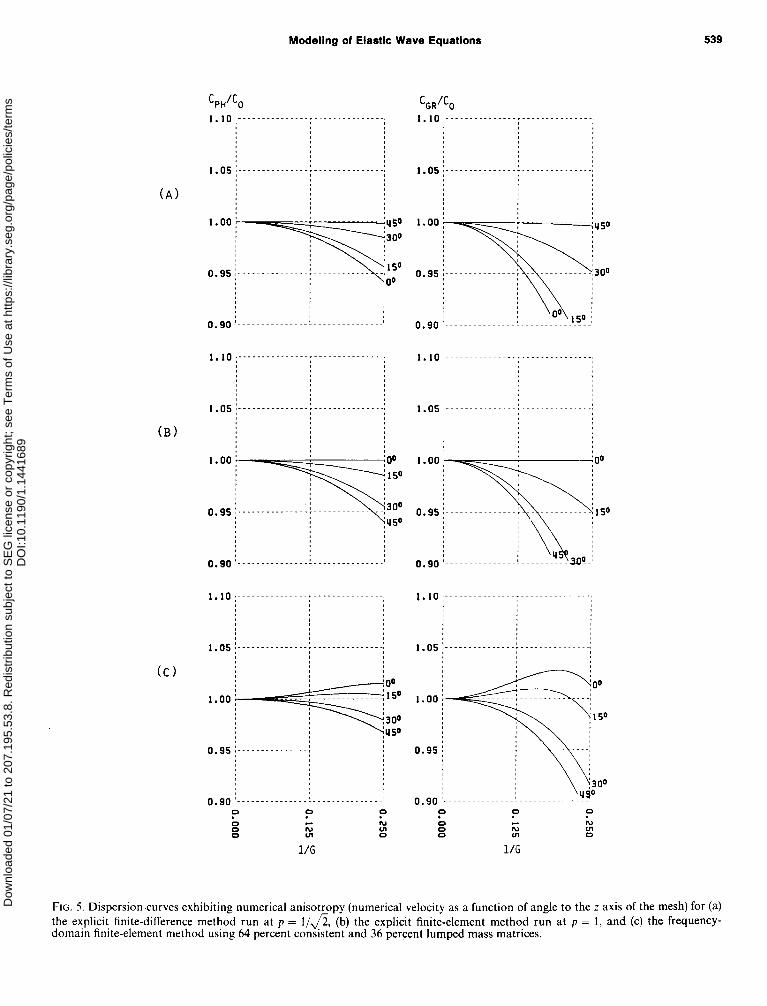
FIG. 5. Dispersion curves exhibiting numerical anisotropy (numerical velocity as a function of angle to the z axis of the mesh) for (a) the explicit finite-difference method run at p = l/s, (b) the explicit finite-element method run at p = 1, and (c) the frequency- domain finite-element method using 64 percent consistent and 36 percent lumped mass matrices.

Dow

nloa

ded

01/0

7/21

to 2

07.1

95.5

3.8.

Red

istr

ibut

ion

subj

ect t

o S

EG

lice

nse

or c

opyr

ight

; see

Ter

ms

of U

se a

t http

s://l

ibra

ry.s

eg.o

rg/p

age/

polic

ies/

term

sD

OI:1

0.11

90/1

.144

1689

540 Marfurt

schemes are said to be only conditionally stable. Other schemes, such as the average acceleration or Newmark scheme (y = l/2, p = l/4), are unconditionally stable, independent of the value of Ax, AZ, and At.

The following observations can be made for finite-difference solutions of the hyperbolic equation.

Accuracy increases with increasing At for central differences, up to the limit defined by the CFL stability condition (for Ax = AZ):

(A)

c,At 1 -I-

‘-Ax fi

POLARITY ERROR ~.OO;_____________

The frequency-domain solution is the lower bound of the explicit central differences scheme as At + 0, and is therefore always less accurate.

Implicit schemes such as the Newmark method ap- proach the accuracy of the frequency-domain solution from below with decreasing At; thus, while the New- mark method guarantees stable solutions, even for p > l/4, the accuracy of such solutions deteriorates so rapidly that they are worthless in most seismic modeling situations.

The accuracy of linear acceleration and Fox- Goodwin schemes closely mimics that of the frequency domain; they are only conditionally stable.

POLARITY ERROR ~~OO;_-_______-_-

2.00,

(D) ;

0.00;

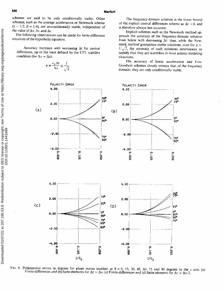
FIG. 6. Polarization errors in degrees for plane waves incident at 8 = 0, 15, 30, 45, 60, 75 and 90 degrees to the z axis. (a) Finite-differences and (b) finite-elements for AZ = Ax. (c) Finite-differences and (d) finite-elements for AZ = AX/~.

Dow

nloa

ded

01/0

7/21

to 2

07.1

95.5

3.8.

Red

istr

ibut

ion

subj

ect t

o S

EG

lice

nse

or c

opyr

ight

; see

Ter

ms

of U

se a

t http

s://l

ibra

ry.s

eg.o

rg/p

age/

polic

ies/

term

sD

OI:1

0.11

90/1

.144

1689

Modeling of Elastic Wave Equations 541

The following observations can be made for finite-element solutions of the hyperbolic equation.

The behavior of the explicit, implicit, and frequency-domain lumped-mass finite-element solutions closely mimics that of finite-differences, with the added benefit that explicit schemes may have larger time steps defined by p = c0 At/Ax < 1 (Figure 4).

Contrary to lumped mass solutions, consistent mass solutions exhibit decreasing accuracy with increas- ing At for central differences. On the other hand, the accuracy of implicit schemes such as the Newmark method increases with At until p = 1. Beyond p = 1 the accuracy deteriorates rapidly, so that one obtains stable, but highly inaccurate results. The linear acceleration and Fox-Goodwin schemes again closely mimic the fre- quency domain solution, changing only slightly with p.

Reduced numerical integration, which obtains in- creased accuracy at reduced cost in static problems (Zienkiewicz, 1977, chap. 11) obtains in general de- creased accuracy over exact numerical integration for the hyperbolic equation.

Averaging the consistent and lumped mass matrices can result in a significant increase in accuracy. A weighted 64 percent consistent, 36 percent lumped mass matrix provides particularly accurate frequency- domain solutions compared to the conventional explicit finite-difference and finite-element solutions (Figure 5). 1 percent error in the group velocity is attained at 26.9 and 21.6 nodes per wavelength for finite-element and finite-difference schemes running at a typical time step corresponding to p = .3, versus 11.5 nodes per wave- length for the mixed mass frequency-domain scheme.

ACCURACY IN NUMERICALLY MODELING THE ELASTIC WAVE EQUATIONS

Principles

In an infinite homogeneous isotropic medium with no damp- ing, the elastic wave equations may be written in the following form

(h + p)V(V - u) + pv * vu - p $ = 0.

Following Bamberger et al (1980), assume wave fields of the form

.Ui(XK, ZK, tJ) z aiK (tj)

= Ai, exp {i(k,x, + k, zK - at,)}; i = 1, 3,

where k, = k sin 8, and k, = k cos 0, as before. Substitution of the wave fields into (8) yields

(A + &Ok: + pk: (h + dkxk,

(h + hkxk; (X + 2p)k; + pk; j’

where po: is the jth eigenvalue and Aj the jth eigenvector of the system of equations. The two eigenvalues can be readily deter- mined to be :

and

po; = (h + 2p)(kf + kf) = (h + 2p)k2,

pw.: = p(kf + k;) = pk2,

corresponding to compressional (P) and shear (S) waves, re- spectively. The two eigenvectors are related to k by

A, x k = 0,

and

A, - k = 0,

implying longitudinal and transverse polarity, respectively. The phase and group velocities of the two solutions are:

c _aop(k)=C _ pv c?k PO ’

J

and

C 57.

_ d%(k) - - = c,,

?k

Thus, an infinite, isotropic elastic medium with no damping is nondispersive. The analysis of accuracies for numerical solu- tions of elastic waves closely mimics that of scalar waves pre- sented previously. The general solution of a mesh containing n nodes entails finding the roots of the determinant of a 2n x 2n (3n x 3n in three dimensions) system of equations. For a homo- geneous mesh, the determinant is again nth order degenerate, such that one need only find the determinant of a 2 x 2 (3 x 3) matrix, yielding two (three) independent modes of propagation approaching those of P- and S-waves at sufficiently small nodal separation. The addition of inhomogeneities in the mesh will yield additional modes of vibration, some physically meaning- ful and some parasitic. For example, the modeling of a semi- infinite 2-D half-space gives an n - 1 degenerate determinant, leading to the solution of a 4 x 4 matrix yielding 4 modes of vibration: one P-wave, one S-wave, one Rayleigh wave, and one purely parasitic mode of vibration.

Discussion of results

Many of the conclusions reached by Bamberger et al (1980) regarding central difference time integration solutions of the elastic wave equations hold equally well for more complicated implicit time integration and frequency-domain solutions. In particular, polarization errors (Figure 6) are independent of the time scheme and Poisson’s ratio, and depend only upon the mesh dimensions. Central difference schemes are, as with the scalar wave equation, only conditionally stable, with

At<J& for finite-differences,

At <” for finite-elements using

L’ P lumped masses,

and

At+&

for finite-elements using

consistent mass matrices,

Dow

nloa

ded

01/0

7/21

to 2

07.1

95.5

3.8.

Red

istr

ibut

ion

subj

ect t

o S

EG

lice

nse

or c

opyr

ight

; see

Ter

ms

of U

se a

t http

s://l

ibra

ry.s

eg.o

rg/p

age/

polic

ies/

term

sD

OI:1

0.11

90/1

.144

1689

542 Marfuti

(A)

1.05 ;-

(B) ;

1.00 k

(cl

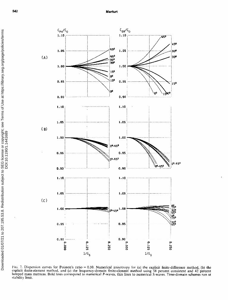
FIG. 7. Dispersion curves for Poisson’s ratio = 0.10. Numerical anisotropy for (a) the explicit finite-difference method, (b) the explicit finite-element method, and (c) the frequency-domain finite-element method using 58 percent consistent and 42 percent lumped mass matrices. Bold lines correspond to numerical P-waves, thin lines to numerical S-waves. Time-domain schemes run at stability limit.

Dow

nloa

ded

01/0

7/21

to 2

07.1

95.5

3.8.

Red

istr

ibut

ion

subj

ect t

o S

EG

lice

nse

or c

opyr

ight

; see

Ter

ms

of U

se a

t http

s://l

ibra

ry.s

eg.o

rg/p

age/

polic

ies/

term

sD

OI:1

0.11

90/1

.144

1689

Modeling of Elastic Wave Equations 543

(A)

(B)

ici

l.lO:-

1.05

l.OC

0.95

0.90

i.ia

1.05

1.00

0.95

0.90

; j-

I I-

’ j- ._.___________________________,

____________._r__...._..______,

1.10

1.05

1.00

0.95

0.90

______:_______________, j,oo-450 3

1.00

______________:_________ ____I 0.95

yuo ._..________._I--___.__-______’ 0.90

_-____----)-_-________--_-;

.3H : lJo_y50

00-1150 .i

1.10 i _________._... _;.______________: 1.10 ;.___ --;- ._._..;

1.05

l/G,

FIG. 8. Dispersion curves for Poisson’s ratio = 0.25 exhibiting numerical anisotropy for (a) the explicit finite-difference method, (b) the exphcrt fimte-element method, and (c) the frequency-domain finite-element method using 56 percent consistent and 44 percent lumped mass matrices. Time-domain schemes run at stability limit.

Dow

nloa

ded

01/0

7/21

to 2

07.1

95.5

3.8.

Red

istr

ibut

ion

subj

ect t

o S

EG

lice

nse

or c

opyr

ight

; see

Ter

ms

of U

se a

t http

s://l

ibra

ry.s

eg.o

rg/p

age/

polic

ies/

term

sD

OI:1

0.11

90/1

.144

1689

544 Marfurl

(A)

1.05;

(B)

1.10

1.05

1.00; ;oo-45

!r=-R 01.00

ho0 o.gs; i ~~ . . . . . 0.95

;1so

0.90 I _...... _______.

1. ,o j ._____...... __.;__---.._“_._..; 1.10

FIG. 9. Dispersion curves for Poisson’s ratio = 0.40 exhibiting numerical dispersion for (a) the explicit finite-difference method, (b) the exphcit finite-element method, and (c) the frequency-domain lumped mass matrices. Time-domain schemes run at stability limit.

finite-element method use 32 percent consistent and 68 percent

Dow

nloa

ded

01/0

7/21

to 2

07.1

95.5

3.8.

Red

istr

ibut

ion

subj

ect t

o S

EG

lice

nse

or c

opyr

ight

; see

Ter

ms

of U

se a

t http

s://l

ibra

ry.s

eg.o

rg/p

age/

polic

ies/

term

sD

OI:1

0.11

90/1

.144

1689

Modeling of Elastic Wave Equations 545

(A)

(B)

Cc)

50

40

30

20

10

0

50

% ?I 40 r s 30 LA

E p 20

z L? D 10 iz ”

0

1X ERROR 0 ' ._----

5X ERROR ____-___-

I

I

;;m;______J _'I

: 5i ERROR --.--._._____.._---. J

50 I

0-l 1 0.0 0.1 0.2

POISSON’S %I0 0.4 05

FIG. 10. Group velocity error curves for the (a) explicit finite- difference method, (b) explicit finite-element method, and (c) frequency-domain finite-element method using the mixed ;ia;;,es in Figure 12. Time-domain schemes run at stability

for square elements (Ax = AZ). In order to compare more easily the accuracy of both P- and

S-waves, the phase velocities, group velocities, and polarity errors of both modes are plotted versus l/G, where G, is the number of nodal points per shear wavelength

1 Ax k,Ax -&=K=y.

The corresponding number of nodes per P wavelength G, is then given by

1 Ax 2rroAx V, Ax V, 1 _=_=-= G, h, V, I/,h,=I/;.,’

In such a fashion, one may compare the relative accuracies of P- and S-waves generated by a source vibrating at one fixed temporal frequency o instead of boundary conditions varying

with spatial frequency k. One may draw the following general conclusions.

(1) For finite-difference solutions of the hyperbolic elastic equa- tions:

The numerical velocities of P-waves are roughly of the same accuracy as those obtained by the numerical solutions of the scalar wave equation. However, the elastic formulation introduces polarity errors in the P- waves that do not exist in the scalar formulation.

For all time integration schemes, shear waves are generally more poorly modeled than P-waves, as can be predicted by their shorter wavelengths.

The phase and group velocities of time-domain solutions approach those of the frequency-domain solu- tions as At + 0.

The velocities of the Newmark method approach those of the frequency-domain solution from below as At+ 0. and they are significantly less accurate than those obtained by the central differences solutions, par- ticularly as At exceeds that of the CFL condition.

Considerable numerical anisotropy is present, with shear-wave phase velocities greater than C,, along the mesh axes and less than C’,, at 45 degrees to the mesh axes for central differences in time (Figures 7a, 8a, 9a).

Shear waves are modeled very poorly at large values of Poisson’s ratio (Figure 10a).

The Fox-Goodwin and linear acceleration tech- niques most closely mimic that of the frequency domain.

(2) For finite-element solutions of the hyperbolic elastic equa- tions :

The behavior of explicit, implicit, and frequency- domain lumped mass finite-element solutions is com- parable to those of finite-differences for Poisson’s ratio less than 0.20 (Figures 7b-7c). However, the numerical shear wave velocities are consistently slower at all angles than the true shear velocity for the finite-element in space, central differences in time explicit scheme.

The finite-element in space/central differences in time explicit scheme is significantly better than that of pure finite-differences for values of Poisson’s ratio be- tween 0.30 and 0.45 (Figures 8b, 9b, lob).

As with the scalar wave equation, consistent mass central differences in time solutions exhibit decreasing accuracy with increasing time step At. The accuracy of the Newmark method increases with At until p z 1, beyond which the accuracy deteriorates rapidly.

Reduced numerical integration schemes generate inferior results to those of full or exact integration.

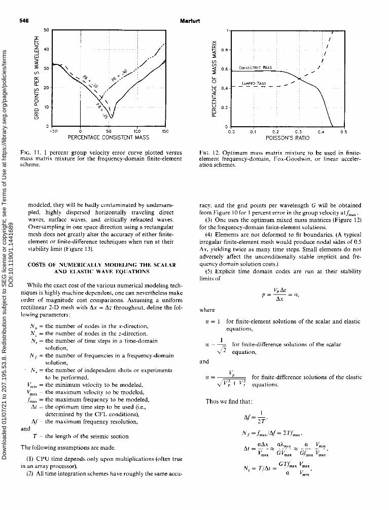
Averaging consistent and lumped mass matrices can result in a significant increase in accuracy. Mixtures of 58 : 42, 56 : 44, and 32 : 68 at values of Poisson’s ratio 0.10, 0.25, and 0.40, respectively, produce particu- larly accurate frequency-domain and Fox-Goodwin or linear acceleration time-domain solutions (Figures 8c, 9c, lOc, 11, 12).

Unequal mesh spacing in the x and z directions can lead to very complicated, undesirable effects if finite energy travels in the poorly sampled direction. While nearly vertically traveling reflecting waves may be well

Dow

nloa

ded

01/0

7/21

to 2

07.1

95.5

3.8.

Red

istr

ibut

ion

subj

ect t

o S

EG

lice

nse

or c

opyr

ight

; see

Ter

ms

of U

se a

t http

s://l

ibra

ry.s

eg.o

rg/p

age/

polic

ies/

term

sD

OI:1

0.11

90/1

.144

1689

Marfur! 546

50

6 = Y 40

9

2 30 In

E E 20

B Q 10

Es

0

1 I

LUMPED flnss ---__-I

o’.o 0:1 0.2 0.'3 0.4 (

POISSON’S RATIO

FIG. 11. 1 percent group velocity error curve plotted versus FIG. 12. Optimum mass matrix mixture to be used in finite- mass matrix mixture for the frequency-domain finite-element scheme.

element frequency-domain, Fox-Goodwin, or linear acceler- ation schemes.

modeled, they will be badly contaminated by undersam- pled, highly dispersed horizontally traveling direct waves, surface waves, and critically refracted waves. Oversampling in one space direction using a rectangular mesh does not greatly alter the accuracy of either finite- element or finite-difference techniques when run at their stability limit (Figure 13).

COSTS OF NUMERICALLY MODELING THE SCALAR AND ELASTIC WAVE EQUATIONS

While the exact cost of the various numerical modeling tech- niques is highly machine dependent, one can nevertheless make order of magnitude cost comparisons. Assuming a uniform rectilinear 2-D mesh with Ax = AZ throughout, define the fol- lowing parameters :

N, = the number of nodes in the x-direction, N, = the number of nodes in the z-direction, N, = the number of time steps in a time-domain

solution, N, = the number of frequencies in a frequency-domain

solution, N, = the number of independent shots or experiments

to be performed, I/min = the minimum velocity to be modeled,

= the maximum velocity to be modeled, 2:; = th e maximum frequency to be modeled,

At = the optimum time step to be used (i.e., determined by the CFL conditions),

Af= the maximum frequency resolution, and

T = the length of the seismic section.

The following assumptions are made.

(1) CPU time depends only upon multiplications (often true in an array processor).

(2) All time integration schemes have roughly the same accu-

racy, and the grid points per wavelength G will be obtained from Figure 10 for 1 percent error in the group velocity atfmar

(3) One uses the optimum mixed mass matrices (Figure 12) for the frequency-domain finite-element solutions.

(4) Elements are not deformed to fit boundaries. (A typical irregular finite-element mesh would produce nodal sides of 0.5 Ax, yielding twice as many time steps. Small elements do not adversely affect the unconditionally stable implicit and fre- quency domain solution costs.)

(5) Explicit time domain codes are run at their stability limits of

V,At p=z=a,

where

a = 1 for finite-element solutions of the scalar and elastic equations,

1 a = -

vb for finite-difference solutions of the scalar equation,

and

a= v, for finite-difference solutions of the elastic 4 vi + v.Z equations.

Thus we find that:

Dow

nloa

ded

01/0

7/21

to 2

07.1

95.5

3.8.

Red

istr

ibut

ion

subj

ect t

o S

EG

lice

nse

or c

opyr

ight

; see

Ter

ms

of U

se a

t http

s://l

ibra

ry.s

eg.o

rg/p

age/

polic

ies/

term

sD

OI:1

0.11

90/1

.144

1689

Modeling of Elastic Wave Equations 547

(A)

1.10

1.05

(B)

1.00 L

1.10

..____..___.._._..____......~~

..__...._..._.~.....-_~_......,

j900

Ii150 7 ‘300 _________-_-__:__--___.. .__I

1150 :oo

_______..___...___...___.....-

_.__________.._____....-------,

.____....__....

(cl [ :3@

1.00;

cGR’cO

l.lO;-

1.05 i-

1.00 k

0.95 I-

0.90 ‘-

1.10 .___....._...._....._......--

0.95

FIG. 13. Same as Figure 8, but with AZ = AX/~.

Dow

nloa

ded

01/0

7/21

to 2

07.1

95.5

3.8.

Red

istr

ibut

ion

subj

ect t

o S

EG

lice

nse

or c

opyr

ight

; see

Ter

ms

of U

se a

t http

s://l

ibra

ry.s

eg.o

rg/p

age/

polic

ies/

term

sD

OI:1

0.11

90/1

.144

1689

548 Marfurt

and

The semi-bandwidth (or dissector) of the effective stiffness matrices that arise in implicit and frequency-domain solutions is of the order N, for the scalar wave equation and 2N, for elastic wave equations for both finite-elements and finite- differences. The number of real arithmetic operations is four times as great in frequency-domain solutions since some com- plex damping must be imposed to obtain stable solutions. Using lower case w for the scalar wave equation and upper case W for the elastic wave equation, one obtains the following CPU work load for the various schemes:

Wfd expl z 7N,N,N,N,,

fe W,XPl z IIN,N,N,N,,

,/e wimp, x w{&, z ION: N, + ION, N, log, (NJN, N, >

w& 2 wg,, z 4ON,’ N, N, + 40N, N, log, (N,)N/ N,,

w:tp, = 11,2N,N:N,N,,

w&r = 20,2N,N,N,N,,

w&, Z WC,,

z lo(2NJ2N, + 10.2N, N, log, (2N,)N, N,,

and

z 40(2N,)*N, N, + 40 2N, N, log, (2N,)N, N,.

One defines

/* wo = W,,pl1 and w, = w:$;dpl

as the work involved in the explicit time-domain finite- difference solutions of the scalar and elastic wave equations, respectively, and

N&IN’* Xc_,, = G&;d,,/G:&xepl

at 1 percent error in the group velocity for each method.

Assuming I/pmsllVPmln = 4 for the scalar problem, and assuming Poisson’s ratio to range between 0.10 and 0.40 and VP,_/ V,_,” = 10 for the elastic problem, one obtains

w&,/w0 z 1.36,

fe Wimpl IWO z o.70w~~f,,/wo

x 0.72 2 + 1.01 log, (0.72N,), 5

fe Wfreq IWO zz o.12wilp,,/wo

z 0.066 2 + 0.066 log, N,, s

wg*,/wo z 0.38,

W&Jwo Z o.low~l,,/wo

2 0.38 2 + 0.19 log, (2N,), s

and

wcLJw0 = o.037w{~,jwo

x 0.0011 2 + 0.0016 log, (0.66N,), 5

where here N, = N{fX,, Finally, one may compare the cost of the full elastic problem

with Poisson’s ratio of 0.25 (V,$L< = 1.73) to that of the scalar acoustic problem (without S-waves) and obtain for 1 percent error in the group velocity

and

CONCLUSIONS

It should be made clear that cost in number of operations to attain a fixed accuracy should not be the only criterion in choosing a particular algorithm. Depending upon the machine and problem sizes, I/O and memory limitations can become the dominant factors. Explicit schemes can be run on 32-bit mac- hines, whereas implicit and frequency-domain schemes which require matrix inversion will require 64 bits. Flexibility is a more nebulous criterion. While the finite-difference schemes are cleaner to code, they may not be easily modified to fit irregular boundaries and topography, or handle weathering zones with high Poisson’s ratio. Frequency-domain codes are substantially more difficult to code but can efficiently model highly hetero- geneous media and include attenuation effects.

The explicit finite-difference and finite-element schemes are comparable when modeling the elastic wave equation for low Poisson’s ratio, but the explicit finite-element scheme is su- perior for Poisson’s ratio greater than 0.25. None of the schemes examined is economically attractive for high Poisson’s ratio (> 0.45) such that one may not model a fluid in an elastic formulation by simply allowing V, to approach zero.

One must yet analyze the accuracy of these schemes in inhomogeneous media and using inhomogeneous meshes. Em- pirically, the author has found finite-elements to model curvi- linear interfaces better and better resolve thin beds and pinchouts than finite-differences. In addition, explicit finite- difference schemes can become unstable when the free surface bounds a medium such as a weathering zone with Poisson’s ratio exceeding 0.4 (Ilan and Loewenthal, 1976). Irregular to- pography which involves homogeneous Neumann boundary conditions may be easily modeled with finite-elements, but not with finite-differences. Finally, Snell’s law and reflection coef- ficients are more a function of numerical phase velocities than the input model velocities.

Of all methods examined, the unconditionally stable frequency-domain finite-element method using a weighted average of consistent and lumped mass matrices provides mini- mum dispersion, neutral amplification, and minimum numeri- cal anisotropy for a fixed cost. Solutions in the frequency domain also place direct control on the frequencies modeled, thereby eliminating high-frequency numerical noise and para- sitic modes of vibration that may arise in higher order time- domain solutions. Through condensation techniques, one may

Dow

nloa

ded

01/0

7/21

to 2

07.1

95.5

3.8.

Red

istr

ibut

ion

subj

ect t

o S

EG

lice

nse

or c

opyr

ight

; see

Ter

ms

of U

se a

t http

s://l

ibra

ry.s

eg.o

rg/p

age/

polic

ies/

term

sD

OI:1

0.11

90/1

.144

1689

Modeling of Elastic Wave Equations 549

economically simulate CDP and well log data and run inter- active models of substrucutres, such as reefs and pinchouts. Attenuation, I/Q, may be prescribed as an arbitrary function of frequency at no extra cost, yielding stable, accurate solutions. Finally, frequency-domain solutions can readily be combined with boundary integral equation techniques to form a hybrid solution.

ACKNOWLEDGMENTS

This work was inspired by recondite conversations with Frank Malone at the Aldridge Laboratory of Applied Geo- physics, Columbia University. Ken Kelly and Dan Whitmore of Amoco Production Company, and Patrick Lailly of INRIA, France, were a continual source of help.

This project was wholly supported by Project MIDAS. The author wisbes to thank the sponsors of this consortium for their support.

REFERENCES

Alford; R. M., Kellv. K. R.. and Boom, D. M., 1974, Accuracy of finite difference modeling of the acoustic wave equation: Geophysics, v.

- 39, p. 834-842. Bambereer. A.. Chavent. G.. and Laillv. P.. 1980, Etude de schemas

numehques pour les equations dk I’elastodynamique lineaire: INRIA (Institut National de Recherche en Informatique et en Automatique), no. 032-79, Le Chesnay, France.

Bathe, K. J., and Wilson, E. L., 1976, Numerical methods in finite element analysis: Englewood Cliffs, NJ, Prentice Hall Inc.

Belytichko, T., and Mullen, R., 1978, On dispersive properties of finite element solutions; in Miklowitz and Achenbach, Eds., Modern problems in elastic wave propagation: New York, John Wiley and Sons.

Brebbia, C. A., 1978, The boundary element method for engineers: New York, Halsted Press, John Wiley and Sons.

Ilan, A., and Loewenthal, D., 1976, Instability of finite difference schemes: Geophys. Prosp., v. 24. p. 43 l-453.

Mullen, R., and Belytichko, T., 1980, Dispersion analysis of finite element semidiscretizations of the two-dimensional wave equation: Dept. of Civil Eng., Northwestern Univ., Evanston, IL.

Pinder. G. F.. and Grav. W. G.. 1977. Finite element simulation in surface andsubsurfacehydrology: New York, Academic Press Inc.

Zienkiewicz, 0. C., 1977, The linite element method: New York, McGraw-Hill Book Co., 3rd ed.

Dow

nloa

ded

01/0

7/21

to 2

07.1

95.5

3.8.

Red

istr

ibut

ion

subj

ect t

o S

EG

lice

nse

or c

opyr

ight

; see

Ter

ms

of U

se a

t http

s://l

ibra

ry.s

eg.o

rg/p

age/

polic

ies/

term

sD

OI:1

0.11

90/1

.144

1689