
Accounting for Electric Vehicles in Air Quality Conformity ... · including Kevin Pete and Wade...
134
TEXAS A&M TRANSPORTATION INSTITUTE COLLEGE STATION, TEXAS TTI: 0-6763 Technical Report 0-6763-1 Accounting for Electric Vehicles in Air Quality Conformity‒Final Report Cooperative Research Program in cooperation with the Federal Highway Administration and the Texas Department of Transportation http://tti.tamu.edu/documents/0-6763-1.pdf
Transcript of Accounting for Electric Vehicles in Air Quality Conformity ... · including Kevin Pete and Wade...

TEXAS A&M TRANSPORTATION INSTITUTE
COLLEGE STATION, TEXAS
TTI: 0-6763
Technical Report 0-6763-1
Accounting for Electric Vehicles in Air Quality Conformity‒Final Report
Cooperative Research Program
in cooperation with the Federal Highway Administration and the
Texas Department of Transportation http://tti.tamu.edu/documents/0-6763-1.pdf


Technical Report Documentation Page 1. Report No. FHWA/TX-15/0-6763-1
2. Government Accession No.
3. Recipient's Catalog No.
4. Title and Subtitle ACCOUNTING FOR ELECTRIC VEHICLES IN AIR QUALITY CONFORMITY—FINAL REPORT
5. Report Date December 2014 6. Performing Organization Code
7. Author(s) Reza Farzaneh, Yuche Chen, Jeremy Johnson, Josias Zietsman, Chaoyi Gu, Tara Ramani, L.D. White, Megan Kenney, and Yue Zhang
8. Performing Organization Report No. Report 0-6763-1
9. Performing Organization Name and Address Texas A&M Transportation Institute College Station, Texas 77843-3135
10. Work Unit No. (TRAIS) 11. Contract or Grant No. Project 0-6763
12. Sponsoring Agency Name and Address Texas Department of Transportation Research and Technology Implementation Office 125 E. 11th Street Austin, Texas 78701-2483
13. Type of Report and Period Covered Technical Report: September 2012–August 2014 14. Sponsoring Agency Code
15. Supplementary Notes Project performed in cooperation with the Texas Department of Transportation. Project Title: Accounting for Electric Vehicles in Air Quality Conformity URL: http://tti.tamu.edu/documents/0-6763-1.pdf 16. Abstract Electric vehicles (EVs) obtain at least a part of the energy required for their propulsion from electricity. The market for EVs, including hybrid, plug-in hybrid, and battery electric vehicles continues to grow, as many new and affordable models have become available in recent years. The proliferation of EVs in the vehicle fleet has implications for energy use and emissions. The mobile source (vehicle exhaust) emissions component is of particular relevance to transportation agencies, especially those in nonattainment and attainment maintenance areas that need to meet transportation conformity requirements. This report presents a framework to incorporate EVs into mobile source emissions estimations. The framework uses the United States Environmental Protection Agency’s Motor Vehicle Emissions Simulator (MOVES) model. It integrates EV driving characteristics, emissions rates, and market penetration information into a MOVES-based emissions inventory analysis. Vehicle activity data collection and drive schedule development, along with in-use emissions measurements, were conducted for a sample of EVs in Texas. Additionally, market penetration scenarios were developed using a consumer choice model. The collected data and market penetration scenarios were then used in the framework to conduct a pilot application for a large county in Texas. The pilot application demonstrated successful use of the framework and showed that including EVs in emissions analyses can potentially have an impact on the overall analysis results specifically for future years. 17. Key Words Electric Vehicles, Mobile Source Emissions, MOVES Model, Portable Emissions Measurement Systems, Drive Schedules, Electric Vehicle Market Penetration, Conformity, Nonattainment, In-Use Emissions
18. Distribution Statement No restrictions. This document is available to the public through NTIS: National Technical Information Service Alexandria, Virginia 22312 http://www.ntis.gov
19. Security Classif.(of this report) Unclassified
20. Security Classif.(of this page) Unclassified
21. No. of Pages 132
22. Price
Form DOT F 1700.7 (8-72) Reproduction of completed page authorized


ACCOUNTING FOR ELECTRIC VEHICLES IN AIR QUALITY CONFORMITY—FINAL REPORT
by
Reza Farzaneh, Ph.D., P.E. Program Manager
Associate Research Engineer Texas A&M Transportation Institute
Yuche Chen, Ph.D.
Assistant Research Scientist Texas A&M Transportation Institute
Jeremy Johnson
Research Specialist Texas A&M Transportation Institute
Josias Zietsman, Ph.D., P.E.
Division Head and Research Engineer Texas A&M Transportation Institute
Chaoyi Gu Assistant Transportation Researcher Texas A&M Transportation Institute
Tara Ramani, P.E.
Assistant Research Engineer Texas A&M Transportation Institute
L.D. White
Associate Research Specialist Texas A&M Transportation Institute
Megan Kenney
Assistant Transportation Researcher Texas A&M Transportation Institute
and
Yue Zhang
Graduate Research Assistant Texas A&M Transportation Institute
Report 0-6763-1 Project 0-6763
Project Title: Accounting for Electric Vehicles in Air Quality Conformity
Performed in cooperation with the Texas Department of Transportation
December 2014
TEXAS A&M TRANSPORTATION INSTITUTE College Station, Texas 77843-3135


v
DISCLAIMER
This research was performed in cooperation with the Texas Department of Transportation
(TxDOT). The contents of this report reflect the views of the authors, who are responsible for the
facts and the accuracy of the data presented herein. The contents do not necessarily reflect the
official view or policies of TxDOT. This report does not constitute a standard, specification, or
regulation. The United States Government and the State of Texas do not endorse products or
manufacturers. Trade or manufacturers’ names appear herein solely because they are considered
essential to the objective of this report.

vi
ACKNOWLEDGMENTS
This project was conducted in cooperation with TxDOT. The authors thank the Project
Monitoring Committee members, Bill Knowles, Ron Hagquist, Laura Norton, and Mollie
Klenzendorf, as well as TxDOT Research and Technology Implementation Division staff,
including Kevin Pete and Wade Odell. The authors acknowledge Martin Boardman, L.D. White,
and Dennis Perkinson of the Texas A&M Transportation Institute for their contributions to this
study, and also gratefully acknowledge the input of Zhenhong Lin and Changzheng Liu of Oak
Ridge National Laboratory.

vii
TABLE OF CONTENTS
Page List of Figures ............................................................................................................................... ix List of Tables ................................................................................................................................. x List of Abbreviations ................................................................................................................... xi Executive Summary ................................................................................................................... xiii Chapter 1: Introduction ............................................................................................................... 1
Background ................................................................................................................................. 1 Research Goals and Approach .................................................................................................... 2 Report Outline ............................................................................................................................. 3
Chapter 2: Background and State of the Practice ..................................................................... 5 Electric Vehicles in the United States ......................................................................................... 5 Factors Influencing EV Adoption ............................................................................................... 7 Electric Vehicles’ Market Penetration ........................................................................................ 9
Market Penetration Forecasting Methods ............................................................................. 10 Market Acceptance of Advanced Automotive Technologies Model .................................... 19
Emissions Impacts of Electric Vehicles .................................................................................... 20 EVs’ Implication for Air Quality and Conformity ................................................................... 27
EVs in Nonattainment Areas ................................................................................................ 27 EV Activity Data for Emissions Modeling ........................................................................... 29
Concluding Remarks ................................................................................................................. 30 Chapter 3: Data Collection and Establishment of EV Emissions Rates ................................ 31
Overview of Approach .............................................................................................................. 31 Development of EV Drive Schedules ....................................................................................... 32
Data Collection Protocol ....................................................................................................... 33 Drive Schedule Data Collection............................................................................................ 36 Development of Drive Schedules ......................................................................................... 37
In-Use Testing of Electric Vehicles .......................................................................................... 44 Data Collection Protocol ....................................................................................................... 44 Test Vehicles ......................................................................................................................... 48
Emissions Data Analysis........................................................................................................... 51 Operating-Mode-Based Emissions Rates ............................................................................. 51 Distance-Based Emissions Rates .......................................................................................... 53
Concluding Remarks ................................................................................................................. 61 Chapter 4: Incorporating EVs into MOVES-Based Emissions Analysis .............................. 63
Framework to Incorporate Electric Vehicles into MOVES-Based Emissions Analysis .......... 63 Pilot Application of Framework ............................................................................................... 64
Methodology ......................................................................................................................... 65 Results ................................................................................................................................... 74
Concluding Remarks ................................................................................................................. 80

viii
Chapter 5: Conclusions .............................................................................................................. 81 References .................................................................................................................................... 85 Appendix A: Operating-Mode-Based EV Energy Consumption and Emissions Rates ....... 93 Appendix B: Aggregated Distance-Based EV Emissions Rates ............................................ 111 Appendix C: Pilot Application Results ................................................................................... 117

ix
LIST OF FIGURES
Page Figure 1. Work Plan Flow Diagram. ............................................................................................... 3 Figure 2. Prediction of HEV, PHEV, and BEV Sales for 2011–2035 (17). ................................... 9 Figure 3. MA3T Model Framework from (26). ............................................................................. 20 Figure 4. Approach for Developing Distance-Based Exhaust Emissions Rates. .......................... 32 Figure 5. QStarz BT-Q1000eX Unit and Its Extended Battery Pack. .......................................... 34 Figure 6. Data Collection Process Flowchart. .............................................................................. 35 Figure 7. Basic Diagram of the Shapes to Determine Location and Area Type. .......................... 38 Figure 8. OpMode Distribution Comparisons for Plug-in Hybrid Vehicles—Arterial,
Statewide Urban, Speed Bin 50 mph. ................................................................................... 42 Figure 9. OpMode Distribution Comparisons for Plug-in Hybrid Vehicles—
Freeway/Highway, Statewide Urban, Speed Bin 50 mph. .................................................... 42 Figure 10. Average Activity OpMode Distribution for Plug-in Hybrid Vehicles—
Freeway/Highway, Statewide Urban. ................................................................................... 43 Figure 11. OpMode Distribution Comparisons for Plug-in Hybrid Vehicles, Hybrid
Vehicles, and Pure Electric Vehicles on Arterial, Statewide Urban Areas........................... 44 Figure 12. Test Route for Driving Tests. ...................................................................................... 46 Figure 13. ECOSTAR Gaseous PEMS. ........................................................................................ 47 Figure 14. PEMS Equipment in Test Vehicle. .............................................................................. 47 Figure 15. AutoEnginuity OBDII Data Logger. ........................................................................... 48 Figure 16. Nissan Leaf Vehicle (Left); Ford Focus Electric Vehicle (Right). ............................. 49 Figure 17. Chevy Volt (Left); Toyota Prius Plug-In (Right). ....................................................... 50 Figure 18. Ford Escape Hybrid (Top Left); Ford Fusion (Top Right); Toyota Camry (Bottom
Left); Toyota Prius (Bottom Right). ..................................................................................... 51 Figure 19. Methodology for Developing Distance-Based Emissions Rates. ................................ 54 Figure 20. CO2 Emission Rates for HEVs on Rural, Arterial Road. ............................................ 55 Figure 21. Aggregated CO2 Emission Rates for the Rural Unrestricted Road Type. ................... 57 Figure 22. Aggregated CO Emission Rates for the Rural Unrestricted Road Type. .................... 58 Figure 23. Aggregated NOx Emission Rates for the Rural Unrestricted Road Type. ................... 58 Figure 24. Aggregated THC Emission Rates for the Rural Unrestricted Road Type. .................. 59 Figure 25. Analysis Framework for Incorporating EVs into Regional Emissions Estimations. .. 64 Figure 26. Electric Vehicles’ Market Penetration Share for Different Scenarios. ........................ 67 Figure 27. Link-Based Hourly Emissions Estimation by MOVESemscalc. ................................ 72 Figure 28. On-Road Exhaust Emissions Estimations for 2014 Scenarios. ................................... 75 Figure 29. CO Emission Rates for HEVs. .................................................................................... 76 Figure 30. On-Road Exhaust Emissions Estimations for 2026 Scenarios. ................................... 77 Figure 31. THC Emission Rate Deterioration Effects and Zero-Mile Emission Effects. ............. 78

x
LIST OF TABLES
Page Table 1. Electric Vehicle Characteristics. ....................................................................................... 6 Table 2. Electric Vehicle Models on the Market. ........................................................................... 7 Table 3. PHEV Market Penetration Forecasting (32). .................................................................. 16 Table 4. US Electric Vehicles Forecasts from Various Models. .................................................. 17 Table 5. Fuel Sources for Electric Power Generation in Texas from (61). .................................. 27 Table 6. Recruited Vehicles by Vehicle Type and Region. .......................................................... 36 Table 7. Recruited Vehicles by Brand. ......................................................................................... 36 Table 8. Speed Bin Definitions for Grouping Micro-Trips. ......................................................... 40 Table 9. Basic Statistics of FWY of PHEVs in Urban Areas. ...................................................... 43 Table 10. Idle and Battery Depletion Testing Conditions. ........................................................... 46 Table 11. BEV Tested Vehicle Specifications. ............................................................................. 49 Table 12. PHEV Tested Vehicle Specifications. .......................................................................... 50 Table 13. Tested HEV Vehicle Specifications. ............................................................................ 51 Table 14. MOVES Variables for VSP Calculation. ...................................................................... 53 Table 15. Electric Vehicle Market Status. .................................................................................... 56 Table 16. Total Miles Driven by Electric Cars. ............................................................................ 60 Table 17. Percentage of Electric Miles Driven. ............................................................................ 60 Table 18. Sample MOVES-Compatible CO2 Emission Table. ..................................................... 61 Table 19. Scenario Developed for Pilot Application. ................................................................... 65 Table 20. Assumptions and Data Sources Used for Pilot Application. ........................................ 70

xi
LIST OF ABBREVIATIONS
ABM Agent-Based Method AEO Annual Energy Outlook ANL Argonne National Laboratory AVID Advanced Vehicle Introduction Decision BEV Battery Electric Vehicle CAA Clean Air Act CARB California Air Resources Board CD Charge Depletion CO2 Carbon Dioxide CO Carbon Monoxide CS Charge Sustaining CV Conventional Vehicle DMV Department of Motor Vehicles DOE Department of Energy EERF Environmental and Emissions Research Facility EPA Environmental Protection Agency EPRI Electric Power Research Institute EV Electric Vehicle FHWA Federal Highway Administration GCV Gasoline Conventional Vehicle GHG Greenhouse Gas GIS Geographic Information System GPS Global Positioning System GREET Greenhouse Gases, Regulated Emissions, and Energy Use in
Transportation HC Hydrocarbon HEV Hybrid Electric Vehicle HGB Houston-Galveston-Brazoria ICE Internal Combustion Engine I/M Inspection and Maintenance IRB Institutional Review Board LA Los Angeles LDV Light-Duty Vehicle

xii
MA3T Market Acceptance of Advanced Automotive Technologies MOVES Motor Vehicle Emission Simulator NA Nonattainment NEDC New European Driving Cycle NOx Nitrogen Oxide NRDC National Resources Defense Council OBDII On-board Diagnostics OpMode Operating Mode ORNL Oak Ridge National Laboratory PEMS Portable Emissions Measurement System PEV Plug-in Electric Vehicle PHEV Plug-in Hybrid Electric Vehicle PM Particulate Matter R&D Research and Development SIP State Implementation Plan SO2 Sulfur Dioxide SUT Source Use Type SUV Sport Utility Vehicle TAMUS Texas A&M University System TDM Travel Demand Model THC Total Hydrocarbons TTI Texas A&M Transportation Institute TxDOT Texas Department of Transportation TxLED Texas Low Emission Diesel UDDS Urban Dynamometer Driving Schedule US United States USEPA United States Environmental Protection Agency VMT Vehicle Miles Traveled VSP Vehicle-Specific Power

xiii
EXECUTIVE SUMMARY
Electric vehicles (EVs), including hybrid, plug-in hybrid, and battery electric vehicles,
differ from conventional gasoline vehicles in that they obtain at least a part of the energy
required for their propulsion from electricity. These vehicles have become more accessible to the
public in recent years, as many new and affordable models have entered the market.
Additionally, infrastructure to support the use of electric vehicles continues to grow, further
increasing their popularity.
The increase in EVs in the vehicle fleet has an impact on energy consumption and
emissions. EVs have the potential for higher energy efficiencies and lower tailpipe emissions
when compared with conventional internal combustion engine vehicles. However, there is
limited research on the emissions implications of increased EVs in the vehicle fleet. In the case
of plug-in electric vehicles (plug-in hybrids and battery electric vehicles), the energy and
emissions associated with the electricity needed to charge the vehicle batteries also need to be
considered.
The main goals of this research were to study the implications of EVs in terms of mobile
source emissions and to develop an approach for incorporating EVs into emissions estimation
procedures. This is a topic of significance to transportation planning agencies, especially those in
nonattainment and attainment maintenance areas needing to meet transportation conformity
requirements. The research team focused on the Texas context, keeping in mind the current
practices of conducting regional emissions analyses using the United States Environmental
Protection Agency’s (USEPA) Motor Vehicle Emission Simulator (MOVES) mobile source
emissions model.
As a first step, the research team conducted a literature review covering key topics related
to the EV market, future market penetration scenarios, and EV impacts on air quality and
emissions. The research team then conducted an extensive vehicle activity data collection
exercise from a sample of EVs in major Texas metropolitan areas. Researchers used these data to
develop representative Texas-specific electric vehicles drive schedules. In-use emissions testing
of EVs was conducted using portable emissions measurements systems to obtain
operating-mode-based emissions rates, which were combined with the drive schedules to obtain
distance-based emissions rates for each type of EV by speed bin and road class. Additionally, a
xiv
set of Texas-specific market penetration scenarios were developed through the application of a
consumer choice model.
A framework was then developed to incorporate the EV parameters (region-specific EV
driving characteristics, emissions rates, and market penetrations) into a MOVES-based emissions
inventory analysis. The Texas-specific data and market penetration scenarios were then used to
conduct a pilot application for Harris County, Texas. The pilot application demonstrated
successful use of the framework and investigated the impact of incorporating EVs on the
modeled on-road exhaust emissions of criteria pollutants or their precursors as well as
greenhouse gases.
In conclusion, this research provided an overview of electric vehicles, the factors
affecting the market penetration of EVs, and the implications for air quality, specifically mobile
source emissions. Texas-specific data on EV activities and emissions were also collected, and a
framework was developed to allow transportation agencies to estimate EVs’ impacts on mobile
source emissions. The intent of the framework is to be flexible and practical, and it uses a
MOVES-based emissions inventory process that is familiar to transportation agencies involved
with air quality and mobile source emissions issues.

1
CHAPTER 1: INTRODUCTION
BACKGROUND
Electric vehicles (EVs), also sometimes termed electrified vehicles, refer broadly to
vehicles that obtain at least a part of the energy required for their operation from electricity. In
this research, EVs were defined as including hybrid electric vehicles (HEVs), plug-in hybrid
electric vehicles (PHEVs), and battery electric vehicles (BEVs). According to the Bureau of
Transportation Statistics and the Alternative Fuel Data Center, EVs accounted for 7.5 percent of
annual new passenger car sales and 0.3 percent of annual new passenger truck sales in 2013
(1,2). With many new and affordable models coming into the market and an increasing
availability of supporting infrastructure, it is expected that the number of EVs in the vehicle fleet
will continue to grow in the future.
By obtaining part or all of the energy needed for propulsion from electricity, EVs can
potentially achieve higher energy efficiencies and result in less exhaust emissions when
compared with conventional vehicles (CVs) powered solely by internal combustion engines.
However, there is limited research on the emissions implications of increased EVs in the vehicle
fleet. Depending on the type of vehicle, the emissions that need to be considered include vehicle
exhaust (tailpipe) emissions as well as the emissions associated with the electricity generation
used for the charging of vehicle batteries in the case of plug-in hybrid and battery electric
vehicles.
From the perspective of transportation agencies, the mobile source emissions component
of (vehicle) exhaust emissions is particularly relevant, especially in nonattainment and
attainment maintenance areas that need to meet transportation conformity requirements. These
agencies have an interest in better understanding and quantifying the emissions and air quality
implications of increasing EVs in the vehicle fleet, and understanding what it means for
transportation and air quality conformity.
The United States (US) Environmental Protection Agency’s (EPA’s) mobile source
emissions estimation model—Motor Vehicle Emission Simulator (MOVES)—forms the basis
for conformity analyses, state implementation plan (SIP) development, and other mobile source
emissions estimations conducted in Texas and much of the United States. The current state of the

2
practice in the use of MOVES does not account for electric vehicles with regard to
location-specific driving characteristics, emissions rates, and market penetration. However,
MOVES provides a platform and has the flexibility to accurately incorporate these aspects into
emissions estimations. Therefore, there is an opportunity to develop methods and approaches by
which EVs can be accurately incorporated into mobile source emissions estimations, including
the transportation conformity analysis framework.
RESEARCH GOALS AND APPROACH
The main goals of this research were to study the implications of EVs in terms of mobile
source emissions, and to develop an approach for incorporating EVs into emissions estimation
procedures, including regional emission inventories. The focus was on the Texas context, and the
research addressed emissions of criteria pollutants and their precursors, including nitrogen oxide
(NOx), hydrocarbons (HCs), and carbon monoxide (CO), as well as greenhouse gases, i.e.,
carbon dioxide (CO2).
This research covered three types of EVs: hybrid electric vehicles, plug-in hybrid electric
vehicles, and battery electric vehicles. HEVs, such as the Toyota Prius, are vehicles that employ
both an internal combustion engine and an electric motor to provide propulsion. The electricity
source for HEVs is from regenerative braking, which is used to recharge the vehicle batteries.
PHEVs, such as the Chevrolet Volt, are powered partly by batteries that are recharged by
plugging into the electric grid and partly by an alternative energy source such as an internal
combustion engine. BEVs, such as the Nissan Leaf, rely solely on electricity from the power grid
(stored in batteries) to provide propulsion. PHEVs and BEVs are also often collectively termed
plug-in electric vehicles (PEVs), as both types of vehicles can be charged by plugging into a
power outlet.
Therefore, while PHEVs and BEVs operating on battery power alone do not contribute to
mobile source emissions, these vehicles indirectly generate emissions through the electricity
generation needed to power PEVs. While the electricity generation component and associated
emissions were not a focus of this project, the broader policy questions arising due to this issue
are briefly covered in this report.
This project was conducted through several distinct activities, as shown in Figure 1. The
initial stages of the project included two parallel tracks. The first focused on gathering

3
background information and conducting a literature review on key topics, followed by
developing Texas-specific EV market penetration scenarios. The second track focused on data
collection for EVs in Texas. This included the collection of real-world activity data to establish
driving characteristics, through development of drive schedules, as well as measurement of EV
exhaust emissions rates using a portable emissions measurement system (PEMS). The research
team then established an analytical framework to incorporate EV market penetration information
along with EV driving characteristics and emissions rates into a MOVES-based analysis
framework. A pilot application was then conducted to demonstrate the use of the framework and
to establish the project’s findings and conclusions.
Figure 1. Work Plan Flow Diagram.
REPORT OUTLINE
Following this introductory chapter, Chapter 2 provides a review of current literature and
the state of the practice with regard to the market for EVs, their emissions impacts, and other
related studies. In addition, different methods for predicting EV market penetration are
presented, including a vehicle consumer choice model used for the pilot application described in
Conclusions
Pilot Application
MOVES-Based Analysis Framework
EV Emissions Rates
EV Market Penetration
EV Driving Characteristics
Background and Literature Review

4
Chapter 4. Chapter 3 then discusses the development of distance-based EV emissions rates using
Texas-specific EV drive schedules (obtained through collection of vehicle activity data) and
in-use measurements of EVs’ emissions rates under real-world driving conditions. Chapter 4
describes the framework developed to incorporate EVs into a MOVES-based analysis and
presents the results for the pilot application conducted for Harris County, Texas. Chapter 5 offers
concluding remarks and identifies possible directions for future research.
5
CHAPTER 2: BACKGROUND AND STATE OF THE PRACTICE
The research team reviewed available literature and conducted a state-of-the-practice
assessment on several topics related to electric vehicles. Specifically, the literature review
presented in this chapter focuses on the background of electric vehicles in the US market, the
factors that influence market penetration, and those studies related to the emissions impacts of
electric vehicles, including HEVs, PHEVs, and BEVs.
ELECTRIC VEHICLES IN THE UNITED STATES
The history of electric vehicles in the US goes back over a hundred years; EVs outsold all
other types of cars between 1899 and 1900 (3). Electric vehicles had many advantages over their
competitors in the early years, as they did not have the vibration, smell, and noise associated
with gasoline cars. Electric vehicles enjoyed success into the 1920s with production peaking in
1912. However, after the 1920s, the proliferation of internal combustion engine (ICE) vehicles
led to the decline of electric vehicles. ICE vehicles allowed for longer ranges of travel, and the
affordable price of gasoline further helped increase their popularity. Electric vehicles almost
disappeared from the market by 1935 but were brought back into market in the 1960s and 1970s
due to concerns regarding conventional vehicles’ tailpipe emissions, as well as concerns
regarding US dependence on imported oil.
Several legislative and regulatory actions have renewed electric vehicle development
efforts in recent years. These include national-level legislation such as the 1990 Clean Air Act
Amendments and the 1992 Energy Policy Act, as well as state-level actions such as the
regulations issued by the California Air Resources Board (CARB) on greenhouse gas emissions
and several states’ zero-emission vehicle requirements (4). The Big Three automobile
manufacturers (General Motors [GM], Ford, and Chrysler) and the Department of Energy
(DOE), as well as a number of vehicle conversion companies, are actively involved in electric
vehicle development through the Partnership for a New Generation of Vehicles (5). Tesla Motors
Inc. is a well-known electric vehicle company in the US, and their Tesla Roadster was
introduced in 2008. According to USEPA, the Roadster can travel 244 mi (393 km) on a single
charge (6). Starting in 2000, car manufacturers began to develop and offer hybrid and electric

6
vehicles to individual consumers. The most popular among these is the Toyota Prius (an HEV),
which had sold more than 3 million vehicles around the world by July 2013 (7).
As mentioned previously, the focus of this project was on three categories of EVs
currently available in the market—HEVs, BEVs, and PHEVs. The project focused on light-duty
vehicles (LDVs) because it is expected that for the short and medium term, the EV market will
be almost exclusively light-duty vehicles. This is consistent with the Energy Information
Administration’s Annual Energy Outlook (AEO) forecasts, which focus exclusively on light-
duty EVs, noting that they have the most significant impact on future fleets (8). Table 1 outlines
the characteristics of the different types of EVs based on various literature sources (5,6,8,9,10).
Table 2 shows a list of the currently available and future/upcoming models as of August 2014.
Table 1. Electric Vehicle Characteristics. Type HEVs PHEVs BEVs
Propulsion • Electric motor drives • ICE
• Electric motor drives • ICE
• Electric motor drives
Energy system • Battery • Ultracapacitor • ICE generating unit
• Battery • Ultracapacitor • ICE generating unit
• Battery • Ultracapacitor
Energy source & Infrastructure
• Gasoline stations • Electric grid charging facilities
• Gasoline stations
• Electric grid charging facilities
Characteristics
• Low emissions at tailpipe and higher fuel economy compared with ICE vehicles
• Dependence on crude oil
• Higher cost compared with ICE vehicles
• Increase in fuel economy and decrease in emissions depending on the power level of motor and battery as well as driving cycle
• Commercially available
• Very low emissions at tailpipe
• Higher fuel economy compared with ICE vehicles
• Higher cost compared with ICE vehicles
• Increase in fuel economy and decrease in emissions depending on the power level of motor and battery as well as driving cycle
• Commercially available
• Zero emissions at tailpipe
• High energy efficiency • No dependence on
crude oils • Limited driving range • High initial cost • Commercially
available
Major issues
• Multiple energy sources’ control, optimization, and management
• Multiple energy sources’ control, optimization, and management
• Battery sizing and management
• Battery and battery maintenance
• Charging facilities

7
Table 2. Electric Vehicle Models on the Market. HEVs PHEVs BEVs
Currently Available
Honda Insight, Civic Hybrid, Toyota Prius, Camry Hybrid, Ford Fusion Hybrid, Mercedes-Benz ML450 Hybrid
BMW i8, Cadillac ELR, Chevy Volt, Fisker Karma, Toyota Plug-In Prius, Ford C-Max Energi, Ford Fusion Energi, Honda Plug-in Accord
BMW-i3, Chevrolet Spark, Coda Automotive, Fiat 500e, Ford Focus, Ford Azure Transit Connection, Honda Fit, Kia Soul, Mercedes-Benz B-Class, Mitsubishi i-MiEV, Nissan Leaf, Scion iQ EV, Smart ForTwo, Tesla Model S, Tesla Roadster, Toyota RAV 4 EV, Wheego LiFe
Future/Upcoming Infiniti Etherea, Subaru Tourer, Fisker Nina, Lexus LC 600h
Fisker Surf, Volvo V60.2, VIA Motors VTrux, Porsche Panamera S E-Hybrid
BYD Auto e6 and VIA Electric Truck, Smart ED, BMW ActiveE
FACTORS INFLUENCING EV ADOPTION
Since electric vehicle models have been increasingly introduced into the market, the sales
of electric vehicles have increased significantly in recent years. Hybrid vehicles are the
fastest-growing segment of the light-duty vehicle market. The number of registered HEVs in the
US grew to nearly 2 million in 2012, and nine of the 10 most fuel-efficient vehicles in the market
today are EVs. Virtually all major vehicle manufacturers and several start-up companies are
offering or are planning to offer plug-in electric vehicles or battery electric vehicles for sale in
the US market. The major factors influencing EV market penetration could be categorized as
energy cost, battery cost and capacity, charging infrastructure, and government policies.
The unpredictability of gasoline prices and energy costs can impact the EV market
penetration. As gasoline prices rise, EVs can be considered an economical option for consumers.
HEVs and PHEVs offer significant reductions in fuel usage, which cuts consumers’ fuel cost,
and BEVs eliminate fuel usage at the pump entirely because they rely solely on a battery for
propulsion. Therefore, the cost of fuel can directly impact the future market of plug-in electric
vehicles.
The future market penetration of plug-in electric vehicles also depends on the
advancement of technology and improvements in plug-in electric vehicle battery technology. The
majority of electric vehicles use lithium-ion batteries because of their high power and energy
density characteristics. However, lithium batteries have limited life cycles that can increase the
costs of vehicle ownership over time. Most automotive manufacturers are planning for a 10-year
battery life span, including expected degradation. Therefore, consumers expect to face
replacement costs for batteries after 10 years of driving. Another limitation related to PHEVs and

8
BEVs is the driving range, particularly for BEVs. Currently, BEVs have shorter ranges per
charge than most conventional vehicles have per tank of gasoline. BEV batteries usually have a
target range of 100 mi, which according to the Federal Highway Administration (FHWA)
accounts for 90 percent of all household vehicle trips in the United States (11). Assuming that
the battery weighs around 250 kg—about 20 to 25 percent of the total weight of typical small
cars—then the battery would give a range of 190 mi in the next 10 years, which is still less than
conventional vehicles’ average travel range of 312 mi.
The development of a charging infrastructure can greatly influence consumers’ decisions
on PHEV/BEV investments and, hence, heavily impact the market penetration of PHEVs and
BEVs. Major recharging options include recharging at home, recharging at commercial
properties (such as shopping centers, schools, etc.), and exchanging depleted batteries with fully
charged ones (12). Government and private sectors have been developing charging stations to
satisfy demand from electric vehicle users. Pike Research estimated that 1.5 million charging
stations will be available in the US by 2017 (13). Many studies have shown that the number of
charging stations per vehicle and the cost of building each station are key determinants of the
adoption rates of EVs (4,5,10,12,13).
Government policies are another important factor that influence EV adoption. Examples
of government policies promoting EV adoption include providing financial incentives to new EV
purchasers, funding research aimed at reducing battery production costs, enforcing more
stringent emissions standards on vehicles, and giving EVs access to high occupancy vehicle
lanes. In the US, the federal government currently is providing tax credits up to $7500 to PHEV
and BEV owners (14). CARB has also established the Clean Vehicle Rebate Project to promote
zero-emission vehicles, which include neighborhood electric, battery electric, plug-in hybrid
electric, and fuel cell vehicles and trucks (15). The US Department of Energy allocated funds
from the American Recovery and Reinvestment Act of 2009 to support and develop more
efficient and cheaper batteries (16). Furthermore, EPA has increased its regulation of the use of
carbon-intensive fuels in transportation and intends to increase regulation of fossil fuels in the
electricity generation mix (9).
Given the above-discussed factors that influence EV adoption, predicting future EV
market penetration is a task involving complex processes and uncertainties. The following

9
section summarizes the most common methods of predicting EV market penetration based on the
literature review.
ELECTRIC VEHICLES’ MARKET PENETRATION
Many research institutes, government agencies, and non-governmental organizations
have studied electric vehicles’ market penetration and developed scenarios and prediction
models based on the factors discussed in the previous section. Among those studies, the electric
vehicle market penetration scenario set developed in the US Department of Energy’s Annual
Energy Outlook is one of the most cited references. In the AEO 2012 report, a projection of EVs’
annual sales was provided for the years 2011 to 2035 (8). As Figure 2 shows, it is predicted that
by 2035, annual sales of HEVs, PHEVs, and BEVs in the US will increase to about 720,000,
190,000, and 90,000, respectively.
In a summary report prepared by Indiana University, the researchers summarized various
projections based on six major global consulting groups’ reports (17). The projections from the
consulting groups suggested that PHEVs’ new vehicle sales would account for 2 percent to
5 percent of all new vehicles by 2020, and 5 percent to 9 percent by 2030. The BEVs’ share of
new vehicle sales is also expected to increase, from 1 percent to 3 percent by 2020 to 8 percent to
10 percent by 2030 (17).
Figure 2. Prediction of HEV, PHEV, and BEV Sales for 2011–2035 (17).

10
Market Penetration Forecasting Methods
This section will describe the various models commonly used by national labs,
universities, and industry to forecast market penetration scenarios for PHEVs, HEVs, and BEVs.
These methodologies include the agent-based method, consumer choice method, diffusion
rate/time series method, and other methods.
Agent-Based Method
The agent-based method (ABM) is a computer-based approach that simulates the actions
and interactions of defined agents to assess their impact on a marketplace. ABM is widely used
to anticipate shifts and evolving trends in the automotive sector, including the introduction of
more sustainable automotive products into the marketplace (18). The agents can be defined as
individuals or organizations. Hence, the method is aptly suited to represent the interactions of a
diverse and varied population of consumers, manufacturers, regulators, and fuel producers and to
understand their impact on an evolving marketplace. ABM vehicle technology market
forecasting studies have defined different agents that operate in the modeling environment, such
as consumers, automakers, policymakers, and fuel suppliers (19).
Sullivan et al. used ABM and found that under a scenario with no federal subsidies, the
PHEV fleet penetration rate would be insignificant, with PHEVs having less than 1 percent of
the market over 10 years. A scenario with an active federal policy including a combination of tax
rebates, PHEV subsidies, and sales tax exemptions could enable a significant increase in the
penetration rate of the PHEV technology. Under more active policy scenarios, PHEVs are
estimated to reach 4 to 5 percent of sales by 2020 (20). The authors noted that the results from
the study depend on many parameters, such as consumer behavior and the turnover rate at which
consumers replace their cars. The results also showed that a PHEV fleet penetration rate of
18 percent would reduce gasoline consumption by 20 percent and decrease fossil carbon
emissions by the same approximate amount.
Sikes et al. used the same method in their study and found the projected PHEV fleet
penetration would range from 2.5 percent to 4 percent for the period from 2015 to 2020 (21).
Sikes et al. assumed that the new technology penetrations and policy conditions would largely
influence the PHEV market penetration. The study also showed that lower vehicle sticker price
would allow PHEVs to be more cost competitive with HEVs and that the HEV market

11
penetration increases under assumptions of lower incremental costs or higher conventional
vehicle operation costs. The study did not provide HEV sales projections for future market
penetration.
Eppstein et al. developed an ABM-based model to estimate the adoption rate of PHEVs
and HEVs using one individual consumer agent and not a household. This model incorporates a
variety of spatial, social, and media effects (22). The study showed that after 10 years, the
penetration rate of HEVs would increase by 25 to 38 percent. Eppstein et al. assumed that each
agent’s age and social network were static, there were uniform daily driving patterns, and there
was availability of daily recharging methods, and they modeled a small subset of vehicle options.
In the study, consumers’ unfamiliarity with PHEV technology, PHEV battery life, battery
replacement cost, long recharging time, future fuel price uncertainty, and short driving range
were assumed to negatively influence the PHEV market penetration. Furthermore, the study
noted that incentive programs such as government tax credits would not have long-term effects
on the fuel efficiency of the fleet.
Consumer Choice Method
The consumer choice method uses a combination of discrete choice models and logit
models to describe individual and collective decision-making. This method is widely used to
model vehicle purchase and holding decisions. The sensitivities of the purchasing decision to the
attributes of the vehicle are obtained through surveys. The attributes estimated in consumer
preference modeling of new vehicle technologies include sensitivity to technology incremental
costs, battery replacement, refueling/charging infrastructure availability, refueling/recharging
time, maintenance costs, and driving range.
The Advanced Vehicle Introduction Decision (AVID) Model was developed by Argonne
National Laboratory (ANL) to predict consumers’ vehicle purchase decisions (23). AVID was
developed using multinomial logit models to predict consumers’ preferences using weighted
scores for individual vehicle technologies and vehicle shares. The researchers of ANL, Santini
and Vyas, used this model to estimate that the HEV adoption rate would increase by 41 percent
with an increase in fuel price of $1.5 per gallon (23). Their study showed that the HEV share
under the unconstrained vehicle production decision was estimated to be 17 percent in 2020 and
23 percent in 2035 to 2050. Vehicle adoption rates were found to be sensitive to gasoline price

12
and HEV technology incremental costs. In the case of a gasoline price increase from $1.50 per
gallon to $3.00 per gallon, HEV sales share increased to 56 percent in 2020 and 64 percent from
2030 to 2050. In the case of an 18 percent increase in HEV incremental costs and gasoline prices
at $3.00 per gallon, HEV sales share was estimated to be between 5 percent and 8 percent from
2020 to 2050. The study considered scenarios including changes in consumer market preference,
vehicle attributes, fuel prices, and technology production decisions. There were 13 vehicle
attributes in their model, including vehicle price, fuel cost, range, battery replacement cost,
acceleration, home refueling, maintenance cost, luggage space, fuel availability, and top speed.
The base case assumption used a gasoline price of $1.50 per gallon and a 7 percent HEV
incremental price increase relative to the CV.
In a Harvard University study, Bandivadekar used discrete choice modeling to estimate
the market penetration rates of EVs (24). Four different scenarios were considered, and the
author estimated that in 2035, the HEV sales would range from 15 percent to 40 percent, and
PHEV sales would range from 0 percent to 15 percent. Bandivadekar noted the initial purchase
price of the vehicle is assumed to be significant in consumers’ choice when selecting electric
vehicles. Charging infrastructure availability is also believed to predict the adoption rate of the
vehicles.
Greene et al. used a nested multinomial logit consumer choice method to examine
numerous scenarios associated with hybrid purchases (25). The scenarios covered multiple time
periods and assumptions regarding competing technologies. The study considered future market
penetration for light-duty diesel vehicles and hybrids, but for this project, only the hybrid market
penetration results were reviewed. The results showed that hybrid vehicles’ purchase rate would
be 4 to 7 percent by 2008 and 15 to 20 percent by 2012 (25).
Sikes et al. also developed a model of consumer choice and estimated that HEV sales
would range from 13 to 17 million in 2020 and PHEV sales would range from 332,975 current
policy cases to 3,569,400 in 2020 (21).
The research team determined that a consumer choice modeling approach would best fit
the requirements and data availability for this study. The team selected the Market Acceptance of
Advanced Automotive Technologies (MA3T) model for this purpose (26).

13
Diffusion Rate and Time Series Method
Time series models examine the process of acceptance of a new invention or product on
the market. The diffusion rate is the speed a product or innovation spreads through the market.
Diffusion rate and time series models seek to capture the life cycle of new products over time.
They have been applied to the prediction of diffusion in a variety of different markets. The most
widely used models are the Bass, Gompertz, and Logistic models. These models have been used
extensively to model innovation diffusion in automotive markets.
Lamberson examined the adoption rate of HEVs using the Bass and Gompertz models.
The study compared diffusion of HEV technologies to that of other automotive innovations and
extrapolated results to the US fleet. Each model provided different results, though the Gompertz
model was found to perform more favorably than the Bass model. Lamberson used a nonlinear
least squares method to estimate the parameters of the Bass and Gompertz models based on
historical monthly US HEV sales (27). In Lamberson’s study, the total market penetration was
estimated to be 1.6 million for the Bass model and 25.7 million for the Gompertz model. The
Bass model estimated that HEV sales would peak in the summer of 2008 and then decline,
whereas the Gompertz model estimated that HEV sales would increase until 2015 and then
decline. Lamberson estimated that in 2015, the annual HEV sales would be 2636 and 1,296,310
based on the Bass and Gompertz models, respectively. Lamberson assumed that government
incentives and regulation would play a major role in HEV adoption.
Cao and Mokhtarian used an extended Bass model with variable market potential to
model HEV market diffusion (28). They included forecasted gasoline prices for the period from
2003 to 2025 and a prediction of consumers’ evolving awareness of HEV technology. The
results showed two peaks in diffusion rate due to first-time HEV purchases and replacement
purchases in year 2023. HEV sales were estimated to reach 510,000 in 2008 and 2 million in
2013. The average annual HEV sales were estimated to be 2.2 million and 2.8 million from 2011
to 2025. In Cao’s study, some of the assumptions considered were that the coefficients of the
Bass model do not change over time, no interaction among vehicle technologies exists, vehicle
technology supply always equals or exceeds demand, and diffusion rate is not affected by
government policies or marketing strategies. The model was tested under different scenarios
such as HEV awareness influence, gasoline price change, and market potential scenarios. In the
scenarios analysis, the market potential was assumed to be around 10 percent of the total US

14
registered vehicles in 2000, and consumer awareness was assumed to increase by 2 percent per
year. Gasoline price was assumed to increase by 25 cents and 50 cents per gallon per year from
2007 onward.
Jeon examined the penetration rate of HEVs, PHEVs, and BEVs until 2030 based on the
Bass diffusion model (29). His model used the concept of successive generations to overcome
the limitations and market saturation problems of the Bass model. The generations were defined
by either a start of new technology carline or a new generation of current carline technology. The
market potential was estimated for each generation as the approximate average sales of the US
vehicle fleet or class in which the technology existed multiplied by the generation period. His
model estimated the annual US sales of HEVs, PHEVs, and BEVs would reach 5 million,
1 million, and 2.1 million, respectively.
Becker reported the rate of electric vehicle adoption using the Bass model under two
gasoline price scenarios accounting for vehicle purchase price and operating costs. In the
baseline scenario, BEVs would have a penetration rate of 3 percent in 2015, 18 percent in 2020,
45 percent in 2025, and 64 percent in 2030 of the total US light vehicle sales (30).
Researchers at the University of California Los Angeles (UCLA) conducted a study on
the market penetration scenarios for electric vehicles for the city of Los Angeles (LA) (31). The
study used standard marketing analysis techniques to forecast the market penetration including a
conjoint survey and Bass diffusion model. The study also looked at cities with comparable
demographics, climate initiatives, and commuting profiles as LA, which included two Texas
cities: Austin and Houston. In the study, researchers interviewed city officials and stakeholders
to understand the local incentives and policies for EV adoption. Researchers forecasted HEVs,
PHEVs, and BEVs as a whole to have a market share of 11.7 percent of the LA fleet by 2020.
Other Methods
Other studies developed market penetration scenarios using various forecast models. A
study by Balducci at the Pacific Northwest National Laboratory examined the market potential
for PHEVs in the US (32). Balducci conducted a literature review and contacted technical
experts and industry leaders to present three market penetration rates for PHEVs for the time
period of 2013 to 2045, as summarized below. Table 3 summarizes the findings of that study.

15
• Hybrid Technology Assessment: In this scenario, PHEV technology adoption was
accelerated as a result of lessons learned through development of hybrid technology, and
the ultimate PHEV share of the hybrid market was based on the penetration definition by
the Electric Power Research Institute (EPRI) and Natural Resources Defense Council
(NRDC). EPRI and NRDC forecasts of hybrid and PHEV market penetration were based
on the choice-based market modeling of customer preference between PHEVs, HEVs,
and conventional vehicle options. The market penetration forecast for this scenario for
PHEV was 9.7 percent by 2023 and 11.9 percent by 2035.
• Research and Development (R&D) Goals Achieved: The second scenario was based on
asking domain experts for the best judgment under a given set of PHEV conditions that
ranged from marginal cost to tax incentives. The second scenario assumed that the major
goals specified in the US DOE’s Plug-In Hybrid Electric Vehicle R&D Plan were
achieved and the tax incentives and positive regulatory environment governing current
hybrid technologies were extended to PHEVs. The DOE goals range from many factors
involved in the development of PHEVs including energy storage, vehicle efficiency
technologies, deployment, engines and fuels, and power electronics. The market
penetration forecast for PHEVs for this scenario was 9.9 percent by 2023 and
27.8 percent by 2035.
• Supply Constrained: The last scenario was based on estimates of the supply capabilities
of automakers and battery manufacturers and assumed that with sufficiently high
consumer demand for EVs generated through various financial incentives and national
energy security priorities and mandates, ultimate market penetration would be limited
only by the idle off-peak capacity of electric infrastructure to meet the demand placed on
it by light-duty vehicles, and near-term penetration would be limited only by the battery
and automotive industries’ ability to meet the surging demand. The scenario forecasted
that PHEVs would reach 26.9 percent by 2023 and 68.4 percent by 2035.

16
Table 3. PHEV Market Penetration Forecasting (32).
A study by Eggers and Eggers developed a choice-based conjoint adoption model to
predict HEV, PHEV, and BEV penetration rates using a consumer preference modeling approach
(33). The results predicted that new vehicle sales would increase to 56.5 percent by 2018 for
hybrid vehicles and 8.4 percent by 2018 for PHEVs. This estimation was based on assumptions
that gas prices would continue to increase, meaning operating costs for ICE cars would rise.
Curtin et al. at the University of Michigan examined the purchasing probability of HEVs
and PHEVs (34). The analysis was based on the results of interviewing a nationally
representative sample of 2513 adults in the US from July to November 2008. The data showed
that while social factors can change consumers’ purchasing decisions, economic incentives
dominate automobile purchasing decisions. The study did not provide market penetration
forecasts but assessed the current state of knowledge of PHEVs among US consumers. Table 5
provides a summary of the market projection forecasts discussed in this document and notes the
stakeholders that cite the forecasts and scope of the projection as part of their studies/literature.

17
Tab
le 4
. US
Ele
ctri
c V
ehic
les F
orec
asts
from
Var
ious
Mod
els.
Est
imat
ion
Mod
el/D
evel
oped
By
Cite
d B
y M
arke
t Pen
etra
tion
Ass
umpt
ions
/Mod
el C
onsid
erat
ions
A
gent
-bas
ed m
odel
s
Sulli
van
et a
l. (2
009)
-
U
nive
rsity
of M
ichi
gan
-
Ford
Mot
or C
ompa
ny
PHEV
: 4–5
% b
y 20
20
-
Fixe
d po
pula
tion
-
Con
stan
t wag
es
-
All
pric
es in
real
dol
lars
Sike
s et a
l. (2
004)
Oak
Rid
ge N
atio
nal L
abor
ator
y (O
RN
L)
PHEV
: 2.5
–4%
for 2
015–
2020
-
G
asol
ine
tax
incr
ease
of 1
.5 c
ents
per
ga
llon
betw
een
2010
and
202
0 -
Po
sitiv
e po
licy
cond
ition
s: sa
les t
ax
exem
ptio
ns a
roun
d 2%
& P
HEV
tax
cred
it ex
tend
ed fr
om 2
015
to 2
020
Epps
tein
et a
l. (2
010)
Col
orad
o St
ate
Uni
vers
ity
HEV
: 25–
38%
for 2
010–
2020
, 30–
60%
for 2
010–
2030
-
Con
sum
ers’
age
and
soci
al n
etw
ork
stat
ic
-
Uni
form
dai
ly d
rivin
g pa
ttern
s and
av
aila
bilit
y of
dai
ly re
char
ging
-
Pe
ople
with
hig
her v
ehic
le m
iles t
rave
led
tend
to b
uy c
ars m
ore
ofte
n
Con
sum
er c
hoic
e m
odel
s
Sant
ini &
Vya
s (20
05)
Arg
onne
Nat
iona
l Lab
orat
ory
H
EV: 5
–8%
for 2
020–
2050
-
18
% in
crea
se in
HEV
incr
emen
tal c
ost
-
Gas
olin
e pr
ice
at $
3.00
per
gal
lon
Ban
diva
deka
r (20
08)
Mas
sach
uset
ts In
stitu
te o
f Te
chno
logy
H
EV: 1
5–40
% in
203
5 PH
EV: 0
–15%
in 2
035
-
Ave
rage
ann
ual g
row
th ra
te o
f new
ve
hicl
e sa
les o
f 0.8
% p
er y
ear
-
Ave
rage
per
-veh
icle
kilo
met
ers t
rave
led
decr
ease
from
0.5
% b
etw
een
2005
and
20
20
-
Con
stan
t fue
l con
sum
ptio
n
Gre
ene
et a
l. (2
004)
-
OR
NL
-
J.D. P
ower
and
Ass
ocia
tes
HEV
: 15–
20%
in 2
012
-
Fuel
eco
nom
y in
crea
se to
38
mpg
, at a
co
st in
crea
se o
f 7–9
%
-
Sam
e H
EV te
chno
logy
per
form
ance
-
To
tal m
arke
t vol
ume
of a
ppro
xim
atel
y 17
.5 m
illio
n un
its
-
33%
bas
elin
e fu
el a
vaila
bilit
y in
200
8

18
T
able
4. U
S E
lect
ric
Veh
icle
s For
ecas
ts fr
om V
ario
us M
odel
s (C
ontin
ued)
.
Est
imat
ion
Mod
el/D
evel
oped
By
Cite
d B
y M
arke
t Pen
etra
tion
Ass
umpt
ions
/Mod
el C
onsi
dera
tions
C
ao a
nd M
okht
aria
n (2
004)
-
U
nive
rsity
of C
alifo
rnia
-
C
alifo
rnia
Dep
artm
ent o
f Tr
ansp
orta
tion
HEV
: inc
reas
e by
2%
per
ye
ar
Gas
olin
e pr
ice
incr
ease
by
25–5
0 ce
nts p
er
gallo
n pe
r yea
r
Bec
ker,
Sidh
u, a
nd T
ende
rich
(200
9)
Uni
vers
ity o
f Cal
iforn
ia, B
erke
ley
EV: 3
% in
201
5, 1
8% in
20
20, 4
5% in
202
5, a
nd
64%
in 2
030
-
Con
serv
ativ
e es
timat
e fo
r bat
tery
life
: a
10-y
ear l
ife b
efor
e ba
tterie
s hol
d an
80%
ch
arge
and
are
no
long
er u
sefu
l -
Pe
r-m
ile c
ost i
s 10
cent
s in
2012
-
Pe
rcen
tage
of l
ight
veh
icle
s pro
duce
d in
U
S re
mai
ns c
onst
ant t
hrou
gh 2
030
Uni
vers
ity o
f Cal
iforn
ia a
t Los
A
ngel
es L
uski
n C
ente
r for
In
nova
tion
(201
1)*
Uni
vers
ity o
f Cal
iforn
ia a
t Los
A
ngel
es
EV: 1
1.7%
by
2020
-
O
il pr
ice
stay
s bel
ow $
100
per b
arre
l -
N
o co
n co
nsid
erat
e su
bsid
ies p
rovi
ded
to
EV se
ctor
-
5%
of m
ulti-
unit
resi
dent
s and
rent
ers w
ill
have
acc
ess t
o ch
argi
ng fa
cilit
y -
C
onsu
mer
atti
tude
s, pr
efer
ence
s, an
d be
havi
or re
mai
n co
nsis
tent
-
H
EV a
nd B
EV le
ave
circ
ulat
ion
afte
r 8
year
s
Oth
er m
odel
s
Bal
ducc
i (20
08)
Paci
fic N
orth
wes
t Nat
iona
l La
bora
tory
PH
EV: 9
.7%
by
2023
and
11
.9%
by
2035
-
PH
EV te
chno
logy
dev
elop
men
t ac
cele
rate
d as
a re
sult
of a
dvan
cem
ents
in
hybr
id te
chno
logy
-
$4
000
mar
gina
l cos
t of P
HEV
tech
nolo
gy
-
40-m
i bat
tery
rang
e

19
Market Acceptance of Advanced Automotive Technologies Model
Based on the review of the existing methodologies, the research team selected the MA3T
model for the pilot application of this study, which is described in Chapter 4. The MA3T model
is a consumer choice model developed by Oak Ridge National Laboratory as a tool for analyzing
scenarios of demand for various automotive powertrain technologies in response to changes in
technologies, infrastructure, energy prices, consumer preferences, and policies (26).
Implemented using Microsoft® Excel for Windows, MA3T simulates market demand by
representing relevant attributes of technologies and consumer behavior, such as technological
learning by doing, range anxiety, access to recharging points, daily driving patterns, and
willingness to accept technological innovation.
Currently, MA3T includes 40 choices, consisting of 20 powertrain technologies for each
of the two vehicle size classes—passenger cars and light-duty trucks. MA3T considers the US
household users of LDVs as the consumer market, which is disaggregated into 1458 segments by
six dimensions: nine census divisions, three residential areas, three attitudes toward novel
technology, three driving patterns, three home recharging situations, and two work recharging
situations. MA3T currently has a study period from 2005 to 2050, which includes a calibration
period of 2005 to 2013, a validation year of 2014, and the projection period of 2015 to 2050. All
prices are expressed in 2012 US dollars.
In its core, MA3T uses the nested multinomial logit method to predict purchase
probabilities among 40 choices by each of the 1458 consumer segments, based on value
components associated with vehicle attributes, driver behavior, infrastructure, energy prices, and
policies (Figure 3). The segment purchase probabilities are translated into market share, sales,
vehicle populations, petroleum use, and greenhouse gas (GHG) emissions. Some of the outputs
serve as feedback signals and, together with other exogenous inputs from various sources, affect
the purchase probabilities. ORNL continuously updates and improves the model (26).

20
Figure 3. MA3T Model Framework from (26).
EMISSIONS IMPACTS OF ELECTRIC VEHICLES
The transportation sector is a major contributor to criteria pollutant and greenhouse gas
emissions in the US, accounting for 28 percent of energy use, 28.1 percent of GHG emissions,
54 percent of CO, 61 percent of NOx, and 24 percent of volatile organic compound (VOC)
emissions in 2012 (35,36,37). Governments around the world are taking steps to address the
energy and air pollution problems caused by transportation activities. One of the strategies being
used for this purpose is to expand penetration of electric vehicles in private and public
transportation sectors (38,39). Because part of their power source is from electricity, electric
vehicles have the potential to achieve higher energy efficiency, reduce fuel consumption, and
mitigate pollutant emissions.
Among the three common types of EVs (HEVs, PHEVs, and BEVs), HEVs are the
closest EV type to conventional vehicles because they still mainly rely on an internal combustion
engine for propulsion, and the electric battery assists the engine and is recharged through
regenerative braking and the internal combustion engine (39). HEVs do not use electricity from a
power grid, i.e., their batteries cannot be charged by plugging into a power outlet. Therefore,
HEVs only produce tailpipe emissions and are similar to conventional vehicles in evaluation of
emissions impacts.
The literature identifies two electric vehicle operating modes to describe the electric
portion of PHEV and BEV operations. Charge depletion (CD) mode is when the battery is

21
charged above a threshold and the vehicle is powered solely by the battery. Charge sustaining
(CS) mode is when the battery is discharged below a threshold and the vehicle is powered
intermittently by a gasoline-powered engine and the battery (39). In the CS mode, tailpipe
emissions will be produced because the internal combustion engine is operating during that
mode. In the CD mode, only grid emissions in generating electricity will be produced. A BEV is
operated solely in the CD mode. A PHEV is operated in the CD mode when the battery is
charged above a threshold, and after that, it is operated in CS mode. Therefore, if only mobile
source emissions are considered—which is the system boundary of transportation air quality
conformity analysis and the objective of this study—EVs could potentially provide benefits in
reducing emissions. If emissions from power grids are included, it is still unclear whether EVs
can produce fewer emissions. Many studies have investigated EV emission impacts at both the
disaggregated level (i.e., individual vehicle) and aggregated level (i.e., regional or national
vehicle fleet).
In a disaggregated-level analysis, EVs’ distance-based emissions rates are calculated and
compared with conventional internal combustion engine vehicles. The emissions evaluated
include both criteria pollutants and GHG emissions. The methods used in obtaining EVs’
distance-based emissions rates are mainly in-use testing using PEMS and automobile operation
simulation models. In studies using PEMS testing methods, distance-based emissions rates are
calculated for vehicles driving on predetermined driving routes. However, the vehicles’ driving
characteristics on the selected routes might not be representative of vehicles driving in that
region. In studies using automobile simulation models, vehicles’ emissions rates have usually
been assessed based on national average drive schedules, such as Federal Test Procedure US06,
which are not representative of region-specific driving characteristics. In addition, emissions
generated in simulation models might deviate from the emissions under real-world driving
situations. Some of the disaggregated-level literature is summarized below.
Graver et al. developed a framework to estimate real-world emissions of a plug-in hybrid
electric vehicle (40). PHEV running exhaust emissions were measured by PEMS, and grid
emissions were based on the electricity consumption data and regional power grid resource mix.
The study reported distance-based emissions rates of CO2, NOx, sulfur dioxide (SO2), and
particulate matter (PM) for running exhaust emissions only and running exhaust plus grid
emissions. The results showed the tested PHEV’s running exhaust emissions rates were 3 percent

22
to 140 percent lower than the corresponding legislation limits. However, when grid emissions
were included, the distance-based emissions rates were similar or higher than the legislation
limits.
Sonntag et al. estimated the relationship between particle number concentrations and
operating characteristics through in-use testing of a diesel-electric bus (41). The operating
characteristics considered were fuel rate, engine speed, bus velocity, and acceleration. The
results indicated that velocity and acceleration were good supplemental prediction variables to
engine characteristic variables. In addition, variables such as driving route, after-treatment
technology, and atmospheric conditions had important impacts on particle numbers.
Robinson and Holmen compared second-by-second particle numbers from a 2010 hybrid
electric vehicle and a comparable conventional vehicle under the same real-world driving
conditions (42). The particle number concentrations were recorded using PEMS. The researchers
found that the average particle number per trip for the HEV was two times higher than the
conventional vehicle. The high particle number emissions from the HEV were mainly due to the
restart behavior at low or stop-and-go driving conditions, which resulted in air quality concerns
in areas such as intersections.
Karabasoglu and Michalek investigated the potential of HEVs, PHEVs, and BEVs to
reduce lifetime GHG emissions under various driving cycles and charging scenarios (43). The
driving cycles considered were the Urban Dynamometer Driving Schedule (UDDS), Highway
Fuel Economy Test, US06, and LA92. The results showed that EVs could achieve most CO2
emissions reductions under urban driving conditions (such as UDDS). At aggressive driving
conditions, such as US06, the benefits of EVs in reducing CO2 emissions diminished
significantly.
Millo et al. analyzed the CO2 emissions benefits and operating cost reduction of a PHEV
and a comparable conventional vehicle under real-world driving conditions (44). They developed
an optimal control model that optimized the PHEV’s driving and charging activities. The running
exhaust emissions and electricity consumptions of the PHEV under the New European Driving
Cycle (NEDC) were simulated using the MATLAB program, and grid emissions were later
calculated based on electricity consumptions. The results indicated the PHEV could reduce 10 to
30 percent of CO2 emissions depending on the electricity generation resource mix.

23
Strecker et al. investigated the well to wheels GHG emissions impacts of converting a
1974 Volkswagen Super Beetle into a plug-in hybrid electric vehicle (45). On-road testing of
emissions was conducted using PEMS. In addition, the Greenhouse Gases, Regulated Emissions,
and Energy Use in Transportation (GREET) model was used to analyze the emissions impacts
based on a lifecycle assessment framework. The results showed significant GHG emissions
reduction could be achieved by converting the conventional vehicle into a PHEV, and additional
GHG emissions reduction could be achieved if the electricity was generated from solar energy.
In a study by EPRI and NRDC, the authors concluded that a PHEV could reduce 40 to
65 percent or more GHG emissions than a conventional vehicle and 7 to 46 percent or more than
an HEV in 2050 if a large number of PHEVs enter the vehicle fleet from 2010 to 2050 (46).
Findings of a study by Thomas suggest that BEVs with a 300-mi range will have higher GHG
emissions compared with conventional vehicles if electricity generation is based on the current
coal technology (47).
Other studies assessed EVs’ emissions impacts at the aggregated level and evaluated the
percentage of emissions reductions due to various EV penetration scenarios at regional or
national levels. The majority of the studies focused on PHEVs and BEVs and evaluated their
emissions impacts due to such things as different market penetrations, power generation resource
mixes, and EV charging scenarios. GHG emissions were the major emission type analyzed in the
current literature, but increasingly studies are looking at EV criteria pollutants’ emissions
impacts. Those studies are summarized below.
Doucette and McCulloch conducted a study that simulated BEVs’ CO2 emissions due to
electricity consumptions in four countries (US, France, China, and India) and compared those
CO2 emissions with similarly configured conventional ICE vehicles (48). They found that in
countries that have high CO2 emissions per unit of electricity (such as China and India), driving a
BEV could potentially lead to higher CO2 emissions compared with a conventional ICE vehicle.
Depending on factors such as BEV battery range and charging infrastructure locations, the
differences in CO2 emissions in driving a BEV could range from −2 percent to 30 percent
compared with a conventional ICE vehicle.
In another study conducted by Doucette and McCulloch, the authors developed a model
that evaluated the prospects of plug-in hybrid electric vehicles in reducing CO2 emissions.
Compared with a conventional ICE vehicle, a plug-in hybrid electric vehicle uses both an ICE
24
and electric motor as power sources (49). Hence, driving a plug-in hybrid electric vehicle could
reduce fuel demand and achieve higher energy efficiency. However, if the CO2 intensity in
electricity is higher than the transportation fuel, driving a plug-in electric vehicle could actually
result in higher CO2 emissions compared with driving a conventional ICE vehicle.
Jansen et al. developed a resource dispatch and emissions model to evaluate plug-in
electric vehicle emission impacts on the western power grid system (50). The study used a
modeled dispatch approach based on a correlation between actual historical dispatch and system
load data to show the emissions impacts associated with various plug-in electric vehicles’
penetration on the western grid. The authors found that PHEV fleet charging behaviors could
determine the electricity demand and power generation source mix for every hour of a day.
Furthermore, hourly power grid emissions were determined by the hourly electricity demand and
power generation source mix. Reduction in grid emissions could be achieved by optimizing
PHEV fleet-wide charging profiles. For example, a 3.5 percent reduction in daily grid CO2
emissions could be achieved by shifting PHEV fleet charging from hours 17–21 to hours 9–17.
Kim and Rahimi studied the future energy loads for a large-scale adoption of plug-in
electric vehicles in the city of Los Angeles and the associated impacts on greenhouse gas
emissions (51). They developed a demand-supply equilibrium model to estimate hourly
greenhouse gas emissions under various electric vehicle adoption scenarios. The results indicate
peak hour charging of plug-in electric vehicles is preferable to off-peak hour charging in the
Los Angeles area due to its unique power generation resource mix in the short run. However, in
the long run, as Los Angeles is shifting the power generation resource mix into more renewable
energy resources, off-peak hour charging of plug-in electric vehicles would provide greater
benefits in reducing greenhouse gas emissions than peak hour charging scenarios.
Ma et al. investigated the true ability of BEVs to reduce GHG emissions through a life
cycle assessment based on various BEV driving patterns in the United Kingdom and California
(52). The driving patterns included different profiles in speed, loading, accessory usage, and
more. The results showed that BEVs can deliver significant driving GHG emissions savings
compared with conventional vehicles under conditions in which the grid GHG intensity used to
charge the batteries is sufficiently low. The study also showed that BEVs perform best relative to
ICE vehicles in terms of driving GHG emissions at low speeds and lightly loaded driving.
25
However, the overall vehicle life cycle emissions are higher for BEVs than ICE vehicles due to
the GHG emissions associated with battery manufacturing.
Sharma et al. quantified the economic and greenhouse gas emission performance of
conventional, hybrid, and battery electric vehicles in Australia (53). The evaluations were based
on Australian-specific driving conditions. They used the Powertrain System Analysis Toolkit
simulation package to simulate economic and greenhouse gas emission performance of various
types of vehicles. The results showed that for large vehicles such as light commercial vehicles,
the BEV had higher life cycle GHG emissions than an equivalent conventional vehicle. For
passenger cars, hybrid electric vehicles were the most effective in terms of cost and GHG
emissions under life cycle assessment.
Silva studied the impacts of introducing HEVs, PHEVs, and BEVs in terms of criteria
pollutants, such as CO, THC, NOx, PM, and CO2 in Portugal (54). The study assumed that the
emissions from each vehicle followed a probability distribution and executed a Monte Carlo
simulation to estimate emissions as a result of various increasing patterns of the EVs’ market
shares. The results indicated that 10 percent to 53 percent reductions in various criteria pollutants
could be achieved with a scenario of 50 percent fleet replaced with EVs. In addition, a 23 percent
reduction in CO2 could be achieved.
Smith conducted research to examine EVs’ impacts on GHG emissions in Ireland
considering factors such as electricity generation and distribution systems and proportion of
vehicle kilometers completed by electric motors (55). The study revealed substantial and
immediate reductions in GHG emissions for urban-type driving cycles with electrified vehicles.
If all urban-mode vehicle kilometers were executed by electric vehicles instead of conventional
ICE vehicles, 25 to 40 percent of GHG emissions from passenger cars could be reduced.
However, electric vehicles were not found to have much potential in reducing GHG emissions
from inter-city travel.
Varga analyzed the CO2 emissions impacts from introducing electric vehicles in the
Romanian market (56). The CO2 emissions were calculated by combining energy consumptions
based on NEDC and power grid generation emissions. A vehicle and power train system-level
simulation tool, AVL CRUISE, was used to estimate energy consumptions. Varga reported that
the average CO2 emissions rate ranged from 90 g/km to 220 g/km depending on the current
power generation resource mix in Romania from 2004 to 2008. The CO2 emissions per km could
26
potentially be reduced by 50 percent to 70 percent if the power were all generated by nuclear
power plants and windmills.
Zhou et al. studied electric vehicles in China from the perspectives of energy
consumptions and GHG emissions (57). A life cycle analysis module, Tsinghua-LCAM, was
used to estimate transportation GHG emissions under the Chinese government’s electric vehicle
development route map plan for 2015 and 2020. The authors showed that the projected EVs in
the fleet could achieve various GHG emissions reductions in different regions given the power
generation resource mix. In general, electric vehicles are expected to reduce 25 percent of the
GHG emissions from the transportation sector by the year 2020.
Finally, the state of Texas leads the United States in electricity generation and
consumption. The electric grid is an integrated system of transmission and distribution lines for
which electricity flows. The US has three electric grids that power the country, and each of them
support a portion of Texas. Electricity demands fluctuate over the course of a day, week, and
season, and the demand is also impacted by location, population, and climate (58,59). Studies
have shown that when PHEVs’ and BEVs’ market penetration rates increase significantly,
consequent recharging activities are expected to significantly change the power demand pattern
(60).
Electricity used to recharge PHEVs and BEVs through electrical grids is generated from
different fuel sources such as coal, natural gas, petroleum, and renewable sources including solar
and wind. The electricity generation mix for recharging impacts the PHEVs’ and BEVs’ overall
emission estimations because each source produces different amounts of emissions. The
electricity generation mix varies by region and time. Table 5 shows examples of the breakdown
of sources for electricity generation in Texas from 2008 to 2010 (61). As shown in Table 5,
natural gas was the second highest source for electricity generation in Texas at 38 percent, which
was very close to the largest source, coal, at 40 percent. Therefore, while PHEVs and BEVs can
potentially reduce overall pollutant emissions compared to conventional vehicles, the emission
reductions greatly depend on the generation mix and charging patterns (60,61,62).

27
Table 5. Fuel Sources for Electric Power Generation in Texas from (61).
Fuel Type 2010 2009 2008 Coal 39.5 % 37.1% 37.4% Natural Gas 38.2% 42.1% 43% Nuclear 13.1% 13.6% 13.2% Wind 7.8% 6.2% 4.9%
EVS’ IMPLICATION FOR AIR QUALITY AND CONFORMITY
The increase in EVs in the vehicle fleet has an impact on tailpipe emissions but also has
broader impacts and implications on local and regional air quality. It is particularly important for
nonattainment and attainment areas to understand the overall impact of EVs on regional
emissions. While EVs in general have lower emissions than conventional internal combustion
vehicles, a portion of emissions associated with PHEV and BEV battery charging are generated
by power plants. These plants are considered point sources, along with other sources such as
chemical plants, refineries, electric utility plants, and other industrial sites.
This study was undertaken in the context of transportation conformity and air quality
issues traditionally dealt with by the transportation sector. Only mobile source emissions were
considered in the transportation conformity context. Because PEVs do not produce tailpipe
emissions when they are in electric mode, the expected increase in the number of these vehicles
in the future means that there will potentially be a notable reduction of mobile source emissions
captured in a conformity determination emissions inventory. However, this reduction may not
necessarily lead to better regional air quality because emissions generated for charging EVs are
not accounted for in transportation air quality conformity determinations. Though beyond the
scope of this study, it is important to note that in a broader air quality perspective, it is essential
to take into consideration the emissions from electricity generation when accounting for EVs’
impacts on air quality, and doing so may have broader future policy implications.
EVs in Nonattainment Areas
Accurately projecting EVs within future fleet mixes is important for metropolitan
planning organizations and districts within nonattainment and attainment maintenance areas to
account for their impact in the air quality planning. Market penetration scenarios can help local
28
and state transportation and air quality agencies plan for future fleet changes and the potential
impact on nonattainment and maintenance areas.
The Clean Air Act (CAA) defines EPA’s responsibilities for protecting public health and
improving the nation’s air quality (63). The CAA requires EPA to set limits on the amount of
certain pollutants, called criteria pollutants, allowed in the air. When the level of any of these
pollutants exceeds the standard in an area, EPA designates that area as being in nonattainment
(NA) for that particular pollutant.
After an area is designated as an NA area by EPA, the state is required to develop a SIP
for the area to implement, maintain, and enforce to reduce the pollutant level in the NA area
down to equal or lower than the standard(s) (64). To accomplish this, for each NA area, the SIP
must:
• Estimate emissions from all sources (mobile, point, and area).
• Establish goals for emissions from each of these sources.
• Develop strategies to attain (or maintain) those goals.
In transportation planning, the primary concern is with on-road mobile source emissions.
The on-road mobile source emissions goal for the SIP is known as the motor vehicle emissions
budget. The total emissions from on-road mobile sources cannot exceed this budget. After the
standard is re-attained by a previously designated NA area, EPA re-designates the area as being
back in attainment, but the area is required to demonstrate how it will maintain this level of air
quality. These previously nonattainment areas are called attainment maintenance areas.
NA and attainment maintenance areas must demonstrate that emissions resulting from
future actions, as identified by the transportation planning and programming process and
documented in the metropolitan transportation plans and transportation improvement programs,
will not exceed the area’s emissions budget. This task is achieved through a process known as
demonstrating transportation conformity, which must be conducted periodically, i.e., within two
years of the initial budget and every four years thereafter, if the plan is updated, or if the SIP
changes. If conformity cannot be demonstrated by a specified deadline, or if the plan expires
before a new one is adopted, the area enters into a conformity lapse. For areas in a conformity
lapse, federal transportation funds cannot be spent on capacity-enhancing projects, though
certain safety, transit, and air quality projects may go forward.

29
EV Activity Data for Emissions Modeling
EPA’s current emissions model, MOVES (in this case, version MOVES2010b), utilizes a
database-centered software framework and a disaggregate emissions estimation algorithm that
includes many new features and provides much more flexibility for input and output options than
the previous-generation emissions model (64). This approach enables MOVES to perform
estimations at different analysis levels such as at the national, state, and local levels. Users of the
model specify vehicle types, time periods, geographical areas, pollutants, vehicle operating
characteristics, and road types being modeled. MOVES also incorporates estimates of energy
consumption along with several coefficients, including heating value, oxidization fraction, and
carbon content. The model was designed to work with databases, allowing for new and updated
data to be more easily incorporated into the model. The default database summarizes emissions
information for the entire US and is drawn from EPA research studies, Census Bureau vehicle
surveys, FHWA travel data, and other federal, state, local, industry, and academic sources.
The MOVES model is equipped with default drive cycles that are based on national-level
data and are thus less reliable in accurately estimating emissions at the local level. The accuracy
of local emission estimates can thus be increased if this information is developed and made
available.
MOVES currently does not adequately account for electric-powered vehicles with regard
to location-specific market penetration, driving characteristics, and emissions rates. The
underlying structure of MOVES is adaptable for new vehicle technologies and has the ability to
include new vehicle types into future vehicle fleets. However, EPA at this point has not
established default emission estimates for EVs. Furthermore, EPA has not defined what
constitutes a hybrid vehicle (65).
The total amount of driving by each vehicle type (i.e., source type vehicle miles traveled
[VMT]) and the vehicles’ driving and emissions characteristics (i.e., drive schedules and
emissions rates) are the key parameters for accurately estimating on-road emissions impacts of
EVs in a MOVES-based framework. In Chapter 3, the two major aspects of quantifying EV
emissions impacts—drive schedules and emissions rates—will be established, and the
methodologies and approaches for each of these will be discussed in detail.

30
CONCLUDING REMARKS
This chapter provided a review of the literature on topics related to electric vehicles and
their impacts on emissions. The research team reviewed characteristics of the major makes and
models of EVs in the US market. They discussed major factors influencing electric vehicles’
adoption rates. The researchers also reviewed major methods of predicting the future market for
electric vehicles used by academic institutes, government agencies, and private companies.
Finally, emissions impacts of EVs and their implications for air quality conformity were
discussed. The research team used this information to develop a framework to incorporate EVs
into a travel-demand-based emissions analysis.

31
CHAPTER 3: DATA COLLECTION AND ESTABLISHMENT OF EV EMISSIONS
RATES
This chapter summarizes the collection of vehicle activity and emissions data from EVs,
and the process of establishing distance-based EVs’ exhaust emissions rates using the collected
data. In MOVES and other mobile source emissions inventory models, emissions are estimated
based on mobile source activity profiles and emissions characteristics (generally in the form of
distance-based emissions rates for on-road activities). While mobile source activity
characteristics are usually obtained through region-specific travel demand models, emissions
characteristics are often developed based on national average driving patterns and emissions
rates contained in the models. In this project, the research team established a set of
distance-based emissions rates for EVs in Texas, based on two sets of collected data: global
positioning system (GPS) data from a sample of EVs in major Texas metropolitan areas, and
tailpipe emissions collected through in-use emissions testing on a sample of EVs using PEMS
equipment.
The distance-based tailpipe emissions were developed for average speed bins on different
road types for HEVs and PHEVs, for CO, NOx, and total hydrocarbons (THCs; criteria pollutants
and precursors), as well as CO2. Data regarding the energy consumption associated with BEVs’
and PHEVs’ battery operations were also collected as part of this research. However, these
results are not presented in detail in this report, which focuses on the mobile source emissions
associated with EVs. The detailed procedures in establishing EV emissions rates are discussed in
the remaining sections of this chapter.
OVERVIEW OF APPROACH
Figure 4 shows an overview of the approach used to establish the MOVES-compatible
Texas-specific emissions rates for EVs. The local distance-based EV emissions rates were
required at each average speed bin and each road type. The process started with obtaining drive
schedules under each average speed bin and road type based on a large-scale activity data
collection exercise for EVs operating in Texas’ major metropolitan areas.
The drive schedules were essentially a series of data points depicting speed over time.
The drive schedules could provide time distribution of operating modes under each average

32
speed bin and road type. In addition, operating-mode-based emissions rates for each individual
EV were measured through in-use testing of a sample of EVs that covered the major models of
EVs in the on-road fleet. The operating mode distributions from the drive schedules were
combined with operating-mode-based emissions rates to generate distance-based emissions rates
(g/mi) for individual vehicles by average speed and road type. Market shares (within each
category, i.e., HEVs/PHEVs) were estimated from historical vehicle sales data and used to
calculate the market-share weighted average emissions rates (g/mi) for each vehicle type
category by average speed and road type. These emissions rates were then converted to a
MOVES-compatible emissions rate table by vehicle type to be used as an input to a previously
developed script, called MOVESemscalc, to estimate regional mobile source emissions using
MOVES. This process is discussed further in Chapter 4.
Figure 4. Approach for Developing Distance-Based Exhaust Emissions Rates.
DEVELOPMENT OF EV DRIVE SCHEDULES
This section describes the approach of developing Texas-specific driving schedules based
on GPS data from a sample of EVs in major Texas metropolitan areas. Drive schedules are
important in quantifying vehicle emissions by providing vehicle speeds over time. Many mobile
source emissions inventory models, such as MOVES, use default drive schedules that are based
on national-level data to generate emissions rates.
There is strong agreement in the scientific community that the driving characteristics of
each area are unique due to different vehicle fleet compositions, driving behaviors, and road

33
network topographies. Therefore, national emissions rates are less reliable in accurately
estimating emissions at the regional level. In the case of EVs, the development of drive
schedules using local vehicle activity data is especially important in order to accurately
characterize and reflect EV operations, which are likely to differ from default drive schedules
contained in MOVES.
Data Collection Protocol
Researchers developed and executed a data collection protocol based on related literature
and the research team’s previous experiences, specifically Texas Department of Transportation
(TxDOT) Report 0-6629-1, Texas-Specific Drive Cycles and Idle Emissions Rates for Using with
EPA’s MOVES Model (66). The test protocol included an unsupervised GPS data collection for
developing the representative drive cycles and a supervised on-road emissions testing to develop
basic emissions rates for EVs.
Data were collected from the following three categories of EVs: HEVs, PHEVs, and
BEVs. Vehicles from these categories were identified, recruited separately for each data
collection effort (drive cycles and emissions), and equipped with data loggers. Researchers
processed and analyzed the data following the MOVES model format for vehicle activity
characterization.
The data collection plan consisted of the following major items:
• Vehicle sample sizes for each vehicle category.
• Technology, methodology, and installation procedures for data collection.
• Required duration of the data collection.
• Procedures for protecting participants’ privacy.
The focus of the data collection effort was on the nonattainment and near-nonattainment
urban areas of Texas: Houston, Dallas–Fort Worth, Austin, and San Antonio. The research team
also recruited a few vehicles from an area in attainment: Bryan–College Station.
Protecting Participants’ Privacy
Because the collected data can potentially reveal an individual’s residence or work place,
the data collection process required procedures to ensure that participants’ identity and location
information were properly protected per instructions of the Title 45 Code of Federal Regulations
Part 46. The research team followed the procedures that were developed under TxDOT Research

34
Project 0-6629 to ensure the privacy of the participants was protected. The team obtained the
necessary approvals from The Texas A&M University System (TAMUS) Institutional Review
Board (IRB) to conduct this project.
Following are the main items in the IRB-approved procedures. The details for each item
have been documented in the report for TxDOT Research Project 0-6629 (66).
• Participant consent.
• Data labeling and storage procedures.
Data Collection Technologies
The research team previously determined that GPS technology would be the best
candidate for collecting speed and location data required for the types of applications being
reviewed. In this project, the research team used the GPS units that were identified and obtained
in TxDOT Project 0-6629, the QStarz BT-Q1000eX Xtreme Recorder (67). Figure 5 shows the
QStarz BT-Q1000eX unit. The details on the characteristics of the Xtreme Recorder are
documented in the TxDOT Project 0-6629 final report (66).
Figure 5. QStarz BT-Q1000eX Unit and Its Extended Battery Pack.
Duration of Data Collection
Based on the findings of TxDOT Project 0-6629, researchers determined that a two-week
period would provide the necessary amount of data (66).
Data Collection Methodology
The data collection process consisted of requiring individual vehicles to record their
normal activity during an extended period of time. The research followed the standardized

35
methodology that was previously developed (66). Figure 6 shows an overall outline of the data
collection methodology.
Figure 6. Data Collection Process Flowchart. Each vehicle was equipped with three GPS data loggers to ensure accuracy in case one
unit malfunctioned or provided erroneous data. Information from each of the three data loggers
was downloaded onto a central server and was merged into one document that was labeled with
variables describing unit number, date of initial activation, and type of vehicle observed.
Vehicle Recruiting for Drive Schedules
Thirty-three vehicles were recruited for GPS data collection. Per the TAMUS
Institutional Review Board requirement, a signed consent form was obtained from each
individual participant as part of the recruiting effort. Participants were compensated $75 for their
participation.
Have Participant Sign Consent Form
Place Data Loggers in Vehicle and Turn On
Retrieve Data Loggers
Download Files from Data Loggers
Export into Spreadsheets
Combine Spreadsheets into a Single File
Label File
Save and Secure File onto Server

36
Vehicle Sample Sizes
A goal of seven to 10 vehicles per vehicle category—HEV, BEV, and PHEV—was set.
Each vehicle was observed for a period of one to two weeks, depending on the level of driving
activity. Table 6 shows the distribution of vehicles observed by vehicle type and area. The
research team recruited 33 individual vehicles for drive cycle data collection. Table 7 shows the
distribution of vehicles recruited by make and model.
Table 6. Recruited Vehicles by Vehicle Type and Region.
Table 7. Recruited Vehicles by Brand. Vehicle Type Nissan Leaf Ford Focus Ford Escape Toyota Prius Chevy Volt Total
HEV – – 6 4 – 10
BEV 11 1 – – – 12
PHEV – – – 7 4 11
Total 11 1 6 11 4 33
Potential participants for the research project were recruited through a variety of
methods. Advertisements were made through the web-based classified listing Craigslist, as well
as the Facebook social media account maintained by the Texas A&M Transportation Institute
(TTI). Direct e-mail messages were distributed to electric vehicle enthusiast groups such as the
North Texas Electric Auto Association from the Dallas–Fort Worth region and the Houston
Electric Auto Association. E-mail messages were also sent directly to the managers of Nissan
and Chevrolet dealerships in the Houston and Dallas–Fort Worth regions in an attempt to reach
owners of Nissan Leaf and Chevy Volt vehicles.
Drive Schedule Data Collection
As mentioned in the previous section, the research team recruited 33 individual vehicles
for drive schedule data collection per previously established procedures. Data collection
followed an unsupervised procedure in which drivers were instructed to follow their normal
Vehicle Type Austin Dallas– Fort Worth
Bryan– College Station Houston San Antonio Total
HEV 2 6 – – 2 10
BEV 8 1 2 1 – 12
PHEV 4 – – 7 – 11
Total 14 7 2 8 2 33

37
driving activities for a period of two weeks. The result of this effort was a database of
second-by-second speed for all participating vehicles.
GPS Assembly Vehicle Installation
As Figure 5 shows, each GPS assembly consisted of three high accuracy GPS logger
units. The installation of the units followed the procedures established in TxDOT Project 0-6629.
The assemblies were placed near the driver seat as a way to maximize the chance for each
GPS unit to self-actuate after detecting vibrations from the physical movement of entering and
leaving the vehicle. The GPS units were equipped with an actuation sensor in order to save
power when the vehicle was not moving.
Data Transferring and Labeling
Data were transferred from each individual GPS unit to a secured central server using the
QSport® software, a proprietary software that came with the GPS unit. The data transfer and file
labeling followed the procedures established in TxDOT Project 0-6629 because the data
contained location information. Only authorized researchers who had valid training through the
Collaborative Institutional Training Initiative had access to the data files.
Development of Drive Schedules
Three GPS units were used on each vehicle to increase the precision and fidelity of the
data, per project director approval. The data processing and analysis were conducted according
to the methodology developed in TxDOT Project 0-6629 consisting of the following general
steps. Details of these steps are documented in the final research report for that project (66).
1. Raw data quality control and validation.
2. Data processing.
3. Data analysis and drive schedule development.
4. MOVES default drive schedule comparison.
The goal of this study was to develop local drive schedules for each of the EV types
according to MOVES road types (rural and urban arterials and freeways/highways). Therefore,
the location information of each second of the data needed to have study area and road type
information assigned. The research team processed the data in a geographic information system

38
(GIS) environment for this purpose. Figure 7 shows an example of the polygons used to
determine location and area type in the GIS.
Figure 7. Basic Diagram of the Shapes to Determine Location and Area Type. The approach used for development of the drive schedules is documented in detail in the
final report for TxDOT Research Project 0-6629 (66). It is based on the methodology that was
used by Eastern Research Group (ERG) to develop MOVES’ default drive cycles for heavy-duty
vehicles (68). The research team made necessary modifications to ERG’s methodology based on
the characteristics of the data from EVs. The approach is based on a process of building up
cycles from individual micro-trips extracted from the GPS data (i.e., the GPS data for all vehicles
were broken down into micro-trips).
All micro-trips were assigned a unique micro-trip identification number, and their time
index for the starting point was set to zero; thus, all micro-trips started at zero seconds. The
micro-trip identification number indicated the type of vehicle and a number showing the order
they were extracted, regardless of their location. The following list shows the format for micro-
trip ID numbers:
• Battery electric vehicle: E + micro-trip order number − E00256.
• Hybrid electric vehicle: H + micro-trip order number − H04257.
• Plug-in hybrid electric vehicle: P + micro-trip order number − P03652.

39
A summary table was created containing the following information for all valid
micro-trips:
• Micro-trip ID.
• Average speed (mph) and duration (seconds).
• Distance traveled (miles).
• Location.
• Road classification (freeway [FWY] or arterial [ART]).
• Area type (rural or urban).
The extracted micro-trips were grouped together in separate data files based on the
following parameters:
• Area and area type − the statewide urban + the statewide rural.
• Average speed bin as shown in Table 8.

40
Table 8. Speed Bin Definitions for Grouping Micro-Trips.
Cases Average Speed Bin (mph)
Speed Bin Definition (mph)
Non-Freeway
A_0 <2.5 <2.5 A_5* 5 2.5≤ & <7.5 A_10 10 7.5≤ & <12.5 A_15 15 12.5≤ & <17.5 A_20 20 17.5≤ & <22.5 A_25 25 22.5≤ & <27.5 A_30 30 27.5≤ & <35 A_40 40 35≤ & <45 A_50 50 45≤ & <55 A_60 60 >55
Freeway
F_0** 2.5 0≤ & <5 F_10 10 5≤ & <15 F_20 20 15≤ & <25 F_30 30 25≤ & <35 F_40 40 35≤ & <45 F_50 50 45≤ & <55 F_60 60 55≤ & <65 F_70 70 >65 F_HS >75 >75
* “A_x” refers to arterial/non-highway roadways at an average speed of x mph. ** “F_x” refers to freeway/highway roadways at an average speed of x mph.
Data Analysis and Drive Schedule Development
The MOVES model converts the speed profile information into a time distribution of
activity unit bins called operating modes (opModes) and then applies appropriate emissions rates
to this distribution.
An ideal drive schedule for a given driving condition is the one that has the maximum
amount of information regarding that condition (i.e., in the context of this study, the one that has
all the observations corresponding to that driving condition). However, using an entire database
of second-by-second speed data is impractical. Therefore, a sub-ideal solution is a continuous
short drive schedule constructed from a limited number of micro-trips, which will closely
represent the ideal solution. This suboptimal solution is easy to implement and is currently used
in MOVES in the form of default drive schedules.
In addition to second-by-second speed data, MOVES lets the user input vehicle activity
information in terms of the equivalent operating mode distribution. This method provides an
opportunity to implement the ideal solution (i.e., all observations) in a practical way. The
research team analyzed the data and developed both ideal and sub-ideal solutions. For a specific

41
speed bin, the ideal solution is the opMode distribution of the entire database for that bin, while
the sub-ideal solution is a relatively short continuous speed profile representing that average
speed bin.
Constructing a sub-ideal solution from a micro-trip database requires a methodology to
examine the representativeness of each micro-trip. The research team decided to use a modified
version of ERG’s approach based on opMode distribution as MOVES’ basic unit of activity.
This approach is documented in detail in the TxDOT Project 0-6629 final report (66).
The final drive schedules and target opMode distributions are submitted to TxDOT in a
database format. By providing this information, the users can pick the solution that fits their
specific applications best. While the target opMode distribution is considered the ideal solution,
it may not be easy to implement for simple analyses. On the other hand, the developed drive
schedules (i.e., cycle) are sub-ideal but easy to implement in most cases.
Comparison to MOVES Default Drive Schedules
The resulting target opMode distributions (i.e., target) and drive schedules (i.e., cycles)
were compared to the default drive schedules of MOVES in terms of their corresponding
distribution of modal operating bins. A single analysis year of 2012 was used for this purpose.
The comparison process consisted of the following steps:
• Establish opMode distribution (target, cycle, and MOVES default):
• Calculate opMode distribution for the target (for opMode comparison purpose only).
• Calculate opMode distribution for the cycle (for opMode comparison purpose only).
• Extract the MOVES default drive schedule that is closest to the target and cycle and
calculate its opMode distribution (for opMode comparison purpose only).
• For all other parameters, use the default values for the target area and vehicle type.
Figure 8 and Figure 9 show an example of the results of this comparison effort. Figure 8
and Figure 9 show opMode distributions for the 50 mph speed bin on arterial/local and
freeway/highway of the same scenario from plug-in hybrid vehicles in the statewide urban area.

42
Figure 8. OpMode Distribution Comparisons for Plug-in Hybrid Vehicles—Arterial,
Statewide Urban, Speed Bin 50 mph.
Figure 9. OpMode Distribution Comparisons for Plug-in Hybrid Vehicles—
Freeway/Highway, Statewide Urban, Speed Bin 50 mph.
Average Drive Schedules
The research team also created the average drive schedules for each vehicle type (i.e.,
combined all the valid observations into a single drive schedule). The purpose of generating the
average drive schedule was to provide information to review the driving behavior at a
macroscopic level. Table 9 and Figure 10 show an example of the results of this effort. Table 9
lists the basic data statistics of plug-in hybrid vehicles on freeways in statewide urban areas.
Figure 10 shows the opMode distributions of both targets and the cycle.
0%
5%
10%
15%
20%
25%
30%
35%
40%
0 1 11 12 13 14 15 16 21 22 23 24 25 27 28 29 30 33 35 37 38 39 40
Freq
uenc
ey P
erce
ntag
e
Operating Mode Bin
Local_TargetLocal_CycleMOVES
0%
5%
10%
15%
20%
25%
30%
35%
40%
0 1 11 12 13 14 15 16 21 22 23 24 25 27 28 29 30 33 35 37 38 39 40
Freq
uenc
ey P
erce
ntag
e
Operating Mode Bin
Local_TargetLocal_CycleMOVES

43
Table 9. Basic Statistics of FWY of PHEVs in Urban Areas. Local Target Local Cycle
Avg. speed (𝒎𝒑𝒉) 46.183 47.422 Std. dev. speed (𝒎𝒑𝒉) 18.819 18.640 Max. speed (𝒎𝒑𝒉) 88.700 81.700 Avg. acceleration (𝒎𝒑𝒉 𝒔−𝟏) 0.696 0.716 Std. dev. acceleration (𝒎𝒑𝒉 𝒔−𝟏) 1.078 1.047 Max. deceleration (𝒎𝒑𝒉 𝒔−𝟏) 10.300 5.000 Max. acceleration (𝒎𝒑𝒉 𝒔−𝟏) 7.200 5.100 Idle (in % of time) 2.800 3.200 Duration (seconds) 122,848 1696 Number of trip segments 17
Figure 10. Average Activity OpMode Distribution for Plug-in Hybrid Vehicles—Freeway/Highway, Statewide Urban.
The research team also found that there were differences among the average opMode
distributions of the three vehicle types investigated in this study. Most significantly, BEVs had a
lower percentage of high-power bins for each average speed group. Instead, they had a higher
percentage of low-power opMode bins, e.g., bins 21 and 30. This effect is potentially a result of
drivers avoiding high-power driving events such as excessive acceleration and higher speeds to
conserve battery charge and extend the driving range. Figure 11 shows an example of the results
of this effort in statewide urban areas for arterial roads.
0%5%
10%15%20%25%30%35%40%45%50%
0 1 11 12 13 14 15 16 21 22 23 24 25 27 28 29 30 33 35 37 38 39 40
Freq
uenc
ey P
erce
ntag
e
Operating Mode Bin
Local_Target
Local_Cycle

44
Figure 11. OpMode Distribution Comparisons for Plug-in Hybrid Vehicles, Hybrid
Vehicles, and Pure Electric Vehicles on Arterial, Statewide Urban Areas.
IN-USE TESTING OF ELECTRIC VEHICLES
EVs’ driving schedules provide an operating mode distribution for each road type and
average speed bin. Additionally, operating-mode-based emissions rates are required in order to
estimate distance-based emissions rates for EVs. In this project, these operating-mode-based
emissions rates were estimated based on in-use testing of EVs, using PEMS equipment. It is
important to note that the drive schedules developed for EVs were not used for the emissions
testing. The in-use testing of EVs was used to obtain emissions rates for each operating mode bin
(in units of g/s of emissions). These rates were then combined with operating mode distributions
obtained from the drive schedules to calculate distance-based emissions rates (in units of g/mi) at
each speed bin for each road type. The detailed process is discussed in the following sections.
Data Collection Protocol
The data collection protocol for developing emissions rates for electric vehicles consisted
of the following major components:
• Test procedures for driving activities.
• Test procedures for idling.
• Data collection equipment and installation procedures.
• Vehicle samples from each vehicle category.
0%5%
10%15%20%25%30%35%40%45%50%
0 1 11 12 13 14 15 16 21 22 23 24 25 27 28 29 30 33 35 37 38 39 40
Freq
uenc
ey P
erce
ntag
e
Operating Mode Bin
EV_TARGET
HEV_TARGET
PHEV_TARGET

45
Test Procedures for Driving Activities
The research team investigated the possibility of testing each vehicle during normal daily
operation, i.e., real-world testing. Researchers found that this approach was not feasible due to
the operational characteristics of the vehicles. These vehicles were operated for only a few hours
or less each day during normal operation, which would not provide enough data to cover all the
desired operating conditions. To ensure that sufficient data were collected for each vehicle, the
driving tests were conducted as a supervised data collection effort at TTI and surrounding areas
in Bryan–College Station. This allowed the team to collect data from each vehicle under
real-world driving conditions while giving the flexibility to collect more data in a more efficient
time frame. Each vehicle was transported to TTI’s Environmental and Emissions Research
Facility (EERF) at the Texas A&M Riverside Campus in Bryan, Texas, for approximately one
week of testing. Both the idling and driving tests were conducted that week.
The procedures for driving activities were developed to ensure that the test vehicles were
put through a test route that would replicate different types of driving conditions, including both
city and highway modes at different speeds. By combining both city and highway driving, the
test route ensured that the vehicle was operated in each MOVES opMode bin in order to
establish the emissions rates. Figure 12 outlines the test route that was followed for the driving
test. The total distance for each test was approximately 31 mi. Each vehicle was driven on the
test route for a minimum of three runs in order to collect sufficient data for establishing the rates.

46
Figure 12. Test Route for Driving Tests. (Source: Google Maps)
Test Procedures for Idling
In addition to the driving test, data were collected while each vehicle was idling under
controlled conditions. The idle testing was conducted inside the environmental chamber at TTI’s
EERF facility under the conditions shown in Table 10. The EERF facility includes an
environmentally controlled test chamber that allows for testing at various conditions.
Researchers selected the test conditions in order to replicate both summer and winter
conditions that an EV might be subjected to in Texas. Each vehicle was placed in the chamber
and allowed to soak in the target temperature for two to three hours prior to the start of the test.
The test began as a cold start test, which was done with the air conditioner (AC) or heater on,
depending on the test condition. When available, the cabin temperature was set to be maintained
automatically at 72 °F. The cold start idling test lasted for 30 minutes, after which time the test
was considered a non-cold-start idling test. The total time for the test was approximately three
hours per condition. During the testing, emissions and battery performance data were collected to
create the emissions rates of each vehicle.
Table 10. Idle and Battery Depletion Testing Conditions. Condition Temperature Relative Humidity Load
Hot Test 95 °F (35 °C) 70% AC
Cold Test 23 °F (−5 °C) N/A Heat

47
Data Collection Equipment
During both driving and idling testing, each vehicle was equipped with instruments to
collect data needed to establish the emissions rates. Two types of data were collected during
testing: emissions and battery/electricity consumption data. TTI’s PEMS was used to collect
emissions data. The PEMS used is an ECOSTAR® system from Sensors Inc. The system, shown
in Figure 13, measures CO, CO2, NOx, and THC, and also includes a flow meter that measures
the volumetric flow of the exhaust. Figure 14 shows the PEMS installed in a test vehicle. The
PEMS was used on each of the PHEVs and HEVs. Because BEVs have no tailpipe emissions,
they were not included in the PEMS data collection.
Figure 13. ECOSTAR Gaseous PEMS.
Figure 14. PEMS Equipment in Test Vehicle.

48
The research team used an on-board diagnostics (OBDII) data logger from
AutoEnginuity® to collect the battery and electricity consumption information from the PHEVs
and BEVs. Figure 15 shows the OBDII data logger used for OBDII data collection. The device
reads and records battery information, such as state of charge and remaining battery power. The
researchers calculated the power consumption of the vehicles for each opMode bin based on the
collected data.
Figure 15. AutoEnginuity OBDII Data Logger.
Test Vehicles
Twelve vehicles were recruited for data collection of in-use testing, including four
vehicles from each target vehicle category. The test vehicles were selected based on availability
and because they were considered to be as representative as possible of the existing overall fleet.
In some vehicle categories, such as the BEVs, where one make of vehicle is more prevalent than
others, multiple vehicles of the same make were recruited for testing. Participants were
compensated $200 for their effort. The following sections describe the details of the recruited
vehicles.
Battery Electric Vehicles
Between 2011 and 2013, approximately 22 different BEV models were produced and
sold in the United States, with 13 additional models available for 2014 (69). Of these models, the
most popular are the Nissan Leaf, Tesla Model S, and Ford Focus Electric (70). These three
vehicles made up almost 92 percent of all BEV sales in 2013, according to available sales data.
Based on these numbers, the research team located three units of the Nissan Leaf and one unit of

49
the Ford Focus Electric for testing. A Tesla was also considered for testing, but the available data
loggers needed to collect the information on the battery performance did not support Tesla
vehicles. Table 11 shows the vehicle specifications of the BEV units that were tested, and Figure
16 includes pictures of a Leaf and the Focus that researchers used in the data collection (71,72).
Table 11. BEV Tested Vehicle Specifications. Vehicle Parameter 2011 Nissan Leaf 2013 Ford Focus Electric
Electric Motor 80 kW, 107 HP 107 kW, 143 HP Battery 24 kWh 23 kWh
Battery Charger 3.3 kW (pre-2013 models) 6.6 kW (2013 model) 6.6 kW
Approximate Range 75 mi 76 mi 2013 Units Sold 22,610 1738
Note: Both Photos Were Taken at the EERF.
Figure 16. Nissan Leaf Vehicle (Left); Ford Focus Electric Vehicle (Right).
Plug-In Hybrid Electric Vehicles
From 2011 to 2013, only eight different PHEV models were available for sale in the
United States, while 10 models were available beginning with model year 2014. PHEVs differ
from BEVs in that they can operate in two different modes:
• Charge depletion mode when the hybrid battery is charged above a threshold and the
vehicle is powered solely by the battery.
• Charge sustaining mode when the battery is discharged below a threshold where the
vehicle cannot be powered solely by the battery. In this mode, the vehicle is powered
intermittently by a gasoline-powered engine and the battery.
The gasoline-powered engine gives PHEVs a much longer range than BEVs, but the
range of their CD mode is shorter than the range of BEVs.

50
The Chevy Volt is the most popular PHEV on the market, having sold over 23,000 units
in 2013, making it 135th in the overall sales numbers of vehicles in the United States, just ahead
of the Nissan Leaf BEV (73). The next most popular PHEVs on the market in 2013 were the
Toyota Prius plug-in and the Ford C-Max. For this project, three Chevy Volts and one Toyota
Prius plug-in were selected to be tested. Table 12 includes the details of the PHEVs tested, and
Figure 17 shows one of the Volts and the Prius that were tested (74,75).
Table 12. PHEV Tested Vehicle Specifications. Vehicle Parameter 2012 Chevy Volt 2011 Chevy Volt 2012 Prius Plug-in
Electric Motor 111 kW, 149 HP 111 kW, 149 HP 60 kW, 80 HP Battery 16 kWh 16 kWh 4.4 kWh
All Electric Range 35 mi 35 mi 15 mi Internal Combustion
Engine 1.4 L, 84 HP 1.4 L, 84 HP 1.8 L, 98 HP
2013 Units Sold 23,094 12,088
Figure 17. Chevy Volt (Left); Toyota Prius Plug-In (Right).
Hybrid Electric Vehicles
HEVs are the most common type among the target vehicle types for this project. Between
2011 and 2014, 134 different HEVs have been available in the United States. The HEV, like the
PHEV, combines an internal combustion engine and a battery-powered electric motor. Unlike the
PHEV models, HEV batteries cannot be charged by an external power source; instead, HEVs
switch between the ICE and the electric motor.
For this project, the research team selected test vehicles to cover different classes of
available hybrid vehicles. Unlike the PHEV and BEV models, where options are limited to
smaller passenger car models, there are different classes of HEVs on the market, including
passenger cars, trucks, and sport utility vehicles (SUVs). The vehicles selected for testing were

51
the Ford Fusion, Toyota Camry, Ford Escape SUV, and Toyota Prius. Table 13 details the
specifications of the hybrid vehicles recruited for testing (76,77,78,79,80). Figure 18 includes
pictures of these vehicles.
Table 13. Tested HEV Vehicle Specifications. Vehicle Parameter 2012
Ford Fusion Hybrid
2012 Toyota Camry
Hybrid
2012 Ford Escape
Hybrid
2011 Toyota Prius
Engine 2.5 L, 156 HP 2.5 L, 156 HP 2.5 L, 155 HP 1.8 L, 98 HP Electric Motor 106 HP 141 HP 94 HP 80 HP
Combined HP (electric motor and ICE engine) 188 HP 200 HP 177 HP 134 HP
Figure 18. Ford Escape Hybrid (Top Left); Ford Fusion (Top Right);
Toyota Camry (Bottom Left); Toyota Prius (Bottom Right).
EMISSIONS DATA ANALYSIS
In this section, operating-mode-based emissions rates from in-use testing of EVs are
reported. Furthermore, distance-based EV emissions rates are calculated based on the
operating-mode-based emissions rates and localized drive schedules developed from GPS data.
Operating-Mode-Based Emissions Rates
In-use testing of EVs provided second-by-second emissions of tested vehicles under
real-world driving conditions. In addition, driving characteristics of each second (i.e.,
instantaneous speed and acceleration) were recorded. Therefore, each second of driving

52
condition was categorized into one MOVES-based operating mode bin. By averaging emissions
under each operating mode, time-based EV emissions rates per operating mode bin were
prepared and later used to establish distance-based EV emissions rates.
The PEMS units used in testing included a vehicle interface connection and GPS unit that
allowed for the collection of second-by-second speed data during all testing. These second-by-
second speed profiles were then used to calculate a second-by-second vehicle-specific power
(VSP), which was then used to determine the opMode that the vehicle was in during a given
second of operation. The emissions data from each second were then averaged for each opMode
bin.
The calculation used to determine the opMode bin was based on the MOVES model. The
equation for VSP is as follows:
𝑉𝑆𝑃 = �𝑆 ∗𝑟𝑜𝑙𝑙𝑖𝑛𝑔𝑇𝑒𝑟𝑚𝐴 + 𝑆 ∗ (𝑟𝑜𝑡𝑎𝑡𝑖𝑛𝑔𝑇𝑒𝑟𝑚𝐵 + 𝑑𝑟𝑎𝑔𝑇𝑒𝑟𝑚𝐶 ∗ 𝑆)
𝑠𝑜𝑢𝑟𝑐𝑒𝑀𝑎𝑠𝑠� + 𝑆 ∗ 𝐴𝑐𝑐. +(9.81
∗ sin(atan(𝐺)) ∗ 𝑆
Where:
• S: Speed (m/s).
• Acc.: Acceleration (m/s).
• rollingTermA, rotatingTermB, dragTermC: variables defined in MOVES based on
vehicle type.
• sourceMass: mass of vehicle (metric ton).
The MOVES variables (rollingTermA, rotatingTermB, dragTermC) are all defined in
MOVES based on the vehicle type. All the vehicles in this test, except for the Ford Escape, were
classified as passenger cars (MOVES source type 21) and therefore had the same MOVES
variable values for these parameters. The Ford Escape was considered a passenger truck
(MOVES source type 31) and, therefore, had slightly different values. The sourceMass of each
vehicle was calculated by taking the vehicle’s curb weight and adding the weight of the PEMS
unit and the driver of the vehicle to give a total sourceMass. The values used in the calculations
for each vehicle are shown in Table 14.
Appendix A presents the emissions rates per operating mode bin for EVs. Although the
focus of this study was on running exhaust emissions, idling emissions rates were also collected
and reported and could be used in future analysis. In addition, the electricity consumptions of

53
BEVs and PHEVs in CD mode were recorded and then used to calculate associated power grid
emissions.
Table 14. MOVES Variables for VSP Calculation. Test Vehicle MOVES Variables
rollingTermA rotatingTermB dragTermC sourceMass 2011 Nissan Leaf 0.156461 0.00200193 0.0049265 1.61206728
2013 Ford Focus Electric 0.156461 0.00200193 0.0049265 1.85564639
2011 and 2012 Chevy Volt 0.156461 0.00200193 0.0049265 1.71503275
2012 Toyota Prius Plug-In 0.156461 0.00200193 0.0049265 1.63250049
2012 Ford Escape Hybrid 0.221120 0.00283757 0.00698282 1.8134623
2012 Ford Fusion Hybrid 0.156461 0.00200193 0.0049265 1.86880056
2012 Toyota Camry Hybrid 0.156461 0.00200193 0.0049265 1.77309257
2011 Toyota Prius Hybrid 0.156461 0.00200193 0.0049265 1.56126494
Distance-Based Emissions Rates
Researchers combined the time distribution of operating mode at each road type and
average speed bin and time-based EV emissions rates at each operating mode bin. The outputs
were distance-based emissions rates (g/mi) at each average speed bin and road type for all
pollutants and vehicle types. Three of the four tested HEVs were passenger cars, which
represented the majority of available hybrid models on the market. The research team applied a
market-share weighted average method to obtain a set of representative emissions rates for HEV
passenger cars. The same procedure was applied to PHEV and BEV passenger cars. HEV
passenger truck emissions rates were from the Ford Escape HEV, which was the only passenger
truck tested. In order to obtain running exhaust emissions rates for PHEV passenger trucks, the
same set of ratios between HEV and PHEV passenger cars were applied to HEV and PHEV
passenger trucks. A limitation of the study is the lack of data for PHEV passenger trucks despite
the research team’s best efforts to find and recruit at least one vehicle from each category. The
main reason for this issue was that PHEV passenger trucks constitute less than 0.01 percent of
the passenger truck fleet in the US.

54
These emissions rates were then converted to a MOVES-compatible emissions rate table
by vehicle type to be used as an input to the MOVESemscalc script. Figure 19 visually shows the
process.
Figure 19. Methodology for Developing Distance-Based Emissions Rates.
Calculating Distance-Based Emissions Rates for Individual Vehicles
Researchers observed that there were not many observations for certain combinations of
average speeds and road types. Enough observations were needed to be able to represent average
vehicle operation conditions for an average drive speed. The research team decided to discard the
observations when there were fewer than 500 seconds of observations for a speed bin. In such
instances, a substitute opMode distribution from other road types was then used to calculate the
emissions rates for that speed bin. The team developed the following criteria to assign a
substitute for such cases:
• Step 1. Use opMode distribution for the same speed bin and road class from the
alternative area type (e.g., if it is rural restricted, then use urban restricted).

55
• Step 2. If Step 1 did not yield a valid opMode distribution, use opMode distribution for
the same speed bin and area type from the alternative road class (e.g., if it is rural
restricted, then use rural unrestricted).
• Step 3. If Steps 1 and 2 did not yield a valid opMode distribution, use opMode
distribution for the same speed bin from the alternative road class and area type (e.g., if it
is rural restricted, then use urban unrestricted).
• Step 4. If none of the above steps work, use the opMode distribution from the MOVES
database for the corresponding speed and road type.
First, the opMode emissions rates for each individual vehicle were combined with the
operating mode distributions developed earlier to generate distance-based emissions rates (g/mi)
for each average speed. Because the actual average speeds of the opMode distributions were
slightly different from the assigned speed of MOVES speed bins, and because not all bins had a
local opMode distribution, the team used a linear interpolation to calculate emissions rates at the
exact assigned speeds of MOVES speed bins. Figure 20 shows a sample of the resulting
distance-based emissions rates for individual vehicles.
Figure 20. CO2 Emission Rates for HEVs on Rural, Arterial Road.
0
100
200
300
400
500
600
700
800
2.5 5 10 15 20 25 30 35 40 45 50 55 60 65 70 75
CO
2 (g/
mi)
Average Speed (mph)
Camry 2012 (HEV)Escape 2012 (HEV)Fusion 2012 (HEV)Prius 2011 (HEV)

56
Calculating Market-Share Weighted Average Emissions Rates for Vehicle Type
MOVES-based emissions estimations require average emissions rates for each vehicle
type. Three vehicle types were included in this study: hybrid electric passenger cars, hybrid
electric passenger trucks, and plug-in hybrid passenger cars.
Researchers assumed that the difference in the age of the vehicles would have only a
minimal impact on their tailpipe emissions. This assumption is consistent with the MOVES age
grouping assumption that vehicles of age 0 to 3 years are in the same age group. To develop
emissions rates that are representative of the average HEV and PHEV in the US market, the team
aggregated the individual vehicles’ emissions rates (g/mi) based on their current market share
(i.e., market-share weighted averages of emissions rates were calculated). This aggregation was
performed on each speed bin.
In the current electric vehicle market, HEVs are the most common electric vehicle type.
However, PHEV and BEV sales are also increasing rapidly. Table 15 provides a summary of
current electric vehicle market shares. The data indicate that the tested vehicles are good
representatives of the current electric vehicles in the US market. As shown in Table 15, the tested
vehicles account for approximately 70 percent and 60 percent of passenger car HEVs and
PHEVs in the US market, respectively (70).
Table 15. Electric Vehicle Market Status. Vehicle Type Market Models Tested Vehicle Share
HEV 134 models until 2014 Prius (58%) Camry (11%) Fusion (3%)
PHEV 8 models from 2011–2013 10 models in 2014
Volt (46.6%) Prius (24.4%)
BEV 22 models from 2011–2014 Leaf (60%) Focus (3.4%)
The market-share-averaged emissions rates were generated for HEV passenger cars,
PHEV passenger cars, and HEV passenger trucks. The rates for the HEV passenger truck were
based on a single HEV Ford Escape tested by the TTI team. The HEV passenger car emissions
factors were based on three HEV passenger cars, and PHEV passenger car values were based on
four PHEV passenger cars.
Figure 21 through Figure 24 show the final distance-based emissions rates for all three
vehicle types on rural unrestricted roads. The results for all road types are included in the

57
appendices. The data indicate that the CO2 and NOx emissions rates for HEV and PHEV
passenger cars are comparable under the rural arterial road type. HEV passenger truck emissions
rates at high speeds (over 40 mph) are significantly higher than those of HEV and PHEV
passenger cars, except for THC. The PHEV passenger car THC emissions at speeds lower than
40 mph are much higher than those of the other vehicles.
Figure 21. Aggregated CO2 Emission Rates for the Rural Unrestricted Road Type.
0
100
200
300
400
500
600
2.5 5 10 15 20 25 30 35 40 45 50 55 60 65 70 75
CO
2 (g/
mi)
Average Speed (mph)
HEV Passenger TruckHEV Passenger CarPHEV Passenger Car

58
Figure 22. Aggregated CO Emission Rates for the Rural Unrestricted Road Type.
Figure 23. Aggregated NOx Emission Rates for the Rural Unrestricted Road Type.
0
5
10
15
20
25
30
35
40
2.5 5 10 15 20 25 30 35 40 45 50 55 60 65 70 75
CO
(g/m
i)
Average Speed (mph)
HEV Passenger TruckHEV Passenger CarPHEV Passenger Car
0
20
40
60
80
100
120
140
2.5 5 10 15 20 25 30 35 40 45 50 55 60 65 70 75
NO
x (g/
mi)
Average Speed (mph)
HEV Passenger TruckHEV Passenger CarPHEV Passenger Car

59
Figure 24. Aggregated THC Emission Rates for the Rural Unrestricted Road Type.
Characterizing PHEVs’ Electric Mode Operation
The distance-based emissions rates calculated for PHEVs in the previous section were
done only for the charge sustaining mode where the vehicle switched between its internal
combustion engine and electric motor. PHEVs produce no tailpipe emissions when driving in CD
mode. A transportation conformity analysis includes only mobile source emissions (i.e.,
emissions associated with electricity production are not included). Therefore, understanding
percentages of PHEV miles driven on electricity is important for estimating PHEVs’ average
distance-based tailpipe emissions rates in CD and CS modes.
A study conducted by the US Department of Energy’s Clean Cities Program estimated
that 70 percent of PHEV miles are driven on electricity. This study was based on travel behavior
data from a 2001 National Household Travel Survey (69). Several online electric vehicle
consumer forums let electric vehicle users report their EV mile reading from the odometer of
their vehicles. These data can be used to develop a relatively accurate estimate of the overall
electric mode percentage for PHEVs in the US market. VoltStats.net collects data from electric
vehicle users and reports the total miles driven, electricity miles driven, and overall fuel
economy (81). Researchers obtained volt usage data for the entire US and three states (Texas,
0
50
100
150
200
250
300
2.5 5 10 15 20 25 30 35 40 45 50 55 60 65 70 75
TH
C (g
/mi)
Average Speed (mph)
HEV Passenger TruckHEV Passenger CarPHEV Passenger Car

60
California, and New York) and analyzed them to estimate the percentage of PHEVs’ electric
mode operation. Table 16 and Table 17 show summary statistics in 2013 of PHEV mileage and
percentage of miles driven on electricity, respectively.
Table 16. Total Miles Driven by Electric Cars. US TX CA NY Min 7 626 193 88 Max 149,090 69,271 78,399 57,500 Mean 16,670 16,467 15,270 16,985 Standard Deviation 12,322 12,707 13,245 12,770
Table 17. Percentage of Electric Miles Driven. US TX CA NY Min 1.4 31.2 20.9 40.4 Max 100 99.8 99.0 97.4 Mean 76.0 74.2 79.8 75.7 Standard Deviation 14.8 18 14.2 16.7
The data indicate that the percentages of miles driven on electricity ranged between
74 percent and 80 percent in the three states, and the national average was at 76.0 percent. Those
real-world observations are consistent with the 70 percent electric miles driven estimated by the
National Renewable Energy Laboratory, whose study was based on nationwide transportation
survey data and considered both electric vehicle battery technology evolvement and users’
driving behaviors (69).
Based on literature and analysis of PHEV user reported data, 76 percent (value of
national average) was selected as the share of PHEVs’ VMT on electricity. This means that
24 percent of PHEVs’ VMT are driven using the ICE, thus producing running exhaust emissions,
while the other 76 percent of PHEVs’ VMT do not produce exhaust emissions. Therefore, after
obtaining the distance-based running exhaust emissions rates for PHEVs, a reduction factor
equaling the share of total PHEV miles driven using the ICE was applied. This factor allowed
equivalent distance-based emissions rates for PHEVs to be established per VMT as a whole,
instead of only for ICE engine operation.
Battery technology is the main factor determining the extent of the full electric/zero-
emission miles of PHEVs. Thus, more miles driven on electricity are expected if higher-capacity
batteries at a reasonable price become available. To determine the future share of the ICE miles
required for an emissions analysis, one needs to make appropriate assumptions regarding the
improvements in the capacity of the batteries used in PHEVs.

61
MOVES-Compatible Emission Table
The calculated market-share averaged emissions rates were converted into MOVES-
compatible emission tables to be input into the MOVESemscalc script. Table 18 shows a sample
of content in the emission table for the MOVESemscalc script.
Table 18. Sample MOVES-Compatible CO2 Emission Table.
pollu
tant
ID
avgS
peed
Bin
ID
proc
essI
D
hour
ID
road
Typ
eID
sour
ceT
ypeI
D
fuel
Typ
eID
rate
PerD
istan
ce
90 1 1 1 3 21 1 279.132 90 2 1 1 3 21 1 231.845 90 3 1 1 3 21 1 208.993 90 4 1 1 3 21 1 273.344 90 5 1 1 3 21 1 258.783 90 6 1 1 3 21 1 242.117 90 7 1 1 3 21 1 266.986 90 8 1 1 3 21 1 276.536 90 9 1 1 3 21 1 283.677 90 10 1 1 3 21 1 318.736 90 11 1 1 3 21 1 352.683 90 12 1 1 3 21 1 332.169 90 13 1 1 3 21 1 311.656 90 14 1 1 3 21 1 309.198 90 15 1 1 3 21 1 328.257 90 16 1 1 3 21 1 349.012
CONCLUDING REMARKS
This chapter summarizes the collection of electric vehicle activity and emissions data
from EVs, as well as the process of establishing distance-based EV exhaust emissions rates using
the collected data. The electric vehicle activity data were collected based on GPS data from a
sample of EVs in major Texas metropolitan areas. The electric vehicle activity data were then
used to develop Texas-specific driving schedules. The research team conducted electric vehicle
in-use emissions testing using PEMS equipment. Finally, the testing results were processed with

62
Texas-specific driving schedules to generate distance-based emissions rates for HEVs, PHEVs,
and BEVs, respectively.

63
CHAPTER 4: INCORPORATING EVS INTO MOVES-BASED EMISSIONS ANALYSIS
This chapter discusses the framework developed to incorporate EVs into a
conformity-type analysis. This involved the integration of EV-specific parameters into a travel-
demand-model-based emission inventory. EPA’s MOVES model has been used widely as a
mobile source emission inventory model in national-, state-, and regional-level air quality
analyses and formed the basis for the framework described in this chapter. Chapter 3 described
how a set of distance-based running exhaust emissions rates were established for HEVs and
PHEVs at each average speed bin and road type based on Texas-specific driving schedules and
in-use emissions testing. Currently, the MOVES model does not have EV emissions rates;
however, the MOVES model has the flexibility to accept user-prepared inputs for more
representative results based on local data. This chapter describes how the EV emissions rates and
activity input were integrated with previously developed MOVES-based emissions estimation
processes. The remainder of this chapter presents the framework for integrating EVs into a
MOVES-based emissions analysis.
FRAMEWORK TO INCORPORATE ELECTRIC VEHICLES INTO MOVES-BASED EMISSIONS ANALYSIS
An overview of the analytical framework is shown in Figure 25. This framework
integrates a vehicle consumer choice model and a MOVES-based emission inventory script to
incorporate EVs into a regional emissions inventory.
EVs’ market penetration (i.e., the number of vehicles or the share of overall fleet) is a key
piece of information required for this process. While historical sales data/trends can be used for
base year analyses, predicting future market penetration is more complex, as described in detail
in Chapter 2. Two of the major factors influencing EVs’ market penetrations are the future
energy price (i.e., cost of fuel) and the presence of any government policies and/or incentives
promoting EVs. In this research, the research team used the MA3T model to project future EVs’
market penetration for a set of future energy prices and government policy scenarios. MA3T is a
well-established automobile market simulation model developed by researchers at the
US Department of Energy’s Oak Ridge National Laboratory (26).

64
Using the EV market shares predicted by the MA3T model, the TTI research team
developed VMT assignments for EVs, which can be used to adjust VMT shares for gasoline
passenger cars and passenger trucks to account for EVs. Similarly, modified EV exhaust
emissions rates were developed (based on the rates generated from in-use testing of EVs) to
include the impact of EVs in the vehicle fleet (Figure 25). The results from the previous step
were combined with other parameters previously prepared by TTI to serve as input data to run a
MOVES-based emission calculation script (MOVESemscalc), also previously developed by TTI
(82).
Figure 25. Analysis Framework for Incorporating EVs into Regional Emissions
Estimations.
PILOT APPLICATION OF FRAMEWORK
The above framework was applied in order to demonstrate its use and to investigate the
impacts of including EVs in the modeled on-road exhaust emissions of greenhouse gases (i.e.,
CO2) and criteria pollutants or their precursors (CO, NOx, and THC) in Harris County, Texas.
Analyses were conducted for the years 2014 and 2026. Harris County is the most populous
county in Texas and encompasses a large part of the Houston metropolitan area. The TTI
research team had access to local data and previous emissions inventories conducted for Harris
County, which were used for the pilot application. The analysis years were selected based on
data availability and to provide a realistic platform to assess the implications of including EVs in
the context of transportation conformity under current and future conditions.

65
Methodology
This section describes the analysis methodology in further detail, including:
• Use of the consumer choice model to predict EV market penetration.
• Adjustments for VMT assignments and EV emissions factors.
• Incorporation into a conformity-type analysis (i.e., integration into emissions inventory).
EV Market Penetration Prediction Using Consumer Choice Model
The research team developed four scenarios to demonstrate how the analytical framework
developed in this study could be used to account for the impact of EVs in regional emission
inventories. Table 19 shows the descriptions of these scenarios. As seen in the table, the
scenarios varied by analysis year, incorporation of EVs, and assumptions used for the MA3T
model where future EV market penetration was projected. The government policy in the model
assumption refers to the $2,500~7,500 tax credit (depending on battery capacity) that the
US government currently offers to the owners of the first 200,000 plug-in electric vehicles (i.e.,
PHEVs and BEVs) from each vehicle manufacturer. It is likely that this tax credit will be
discontinued around the year 2020, and this was the assumption employed for most 2026
scenarios. However, an Extended Incentives 2026 scenario was also included to study the impact
of extending the government tax credit until the end of 2026.
Table 19. Scenario Developed for Pilot Application.
Scenario Analysis
Year EVs in Fleet EV Market-Share Source
Assumptions in MA3T Model
Energy Price Source
Government Policy on
PEVs
Base Case 2014 2014 No N/A – – EV 2014 2014 Yes Pre-2014: Historical Sales Data – – Base Case 2026 2026 No N/A – –
High Oil Price 2026 2026 Yes
Pre-2014: Historical Sales Data 2014–2026: Projections from MA3T Model
AEO 2014 High Oil Price
Tax Credits until 2020
Medium Oil Price 2026 2026 Yes
Pre-2014: Historical Sales Data 2014–2026: Projections from MA3T Model
AEO 2014 Reference Oil Price
Tax Credits until 2020
Low Oil Price 2026 2026 Yes
Pre-2014: Historical Sales Data 2014–2026: Projections from MA3T Model
AEO 2014 Low Oil Price
Tax Credits until 2020
Extended Incentives 2026 2026 Yes
Pre-2014: Historical Sales Data 2014–2026: Projections from MA3T Model
AEO 2014 Reference Oil Price
Tax Credits until 2026

66
The research team ran the MA3T model using inputs and assumptions described in Table
19. The energy prices were based on various price scenarios of the AEO 2014 report. AEO’s
reference oil price case assumes trends that are consistent with historical and current market
behavior, technological and demographic changes, and current laws and regulations. The AEO’s
high and low oil price cases are predicted based on trends that would lead to high and low future
oil prices. Figure 26 shows the expected market share of EVs as the MA3T model predicted. The
results indicate that passenger car HEVs’ market shares will peak in the year 2020 and then start
declining for all scenarios. In addition, the projected passenger truck HEV market shares will
increase from 2014 to 2026; however, after 2020, the projected market share will remain flat. On
the other hand, the results show that the market shares of plug-in electric vehicles, including
PHEVs and BEVs, will experience a sharp decrease around 2020, which is the year that tax
credits are planned to be discontinued. The only exception is under the extended incentive
scenario, where the projected market shares for BEVs and PHEVs continue to increase.

67
Figure 26. Electric Vehicles’ Market Penetration Share for Different Scenarios.
Adjustment for EV VMT Shares and EV Emissions Factors
Understanding electric vehicles’ market penetration was only the first step in evaluating
their emissions impact. In order to use the MOVESemscalc script, additional steps required
included creating modified emission factors representing a combination of conventional vehicle
and EV rates as well as apportioning the VMT between the vehicle types. Therefore, two
additional processes were required: EV VMT assignment and EV emissions rates adjustments.
These are described in further detail below.

68
• EV VMT Shares. The MOVESemscalc script calculated link-level emissions estimates
by multiplying hourly link-level VMT with emissions rates for each vehicle type and then
aggregating them for 24 hours of a day and over all links. The link-level VMTs were
designated for each MOVES source use type (SUT). In the EV VMT share development
process, link-level VMTs for all SUTs remained unchanged, except for the gasoline
passenger car and gasoline passenger truck categories. For these two SUTs, link-level
VMT from a travel demand model was redistributed from gasoline conventional vehicle
(GCV) only to GCV, HEV, PHEV, and BEV categories. The assumption in this process
was that consumers purchase an electric car/truck as a substitute to a gasoline passenger
car/passenger truck. The calculation steps as applied to gasoline passenger cars and
gasoline passenger trucks were as follows:
o Step 1: Obtain EV market-share data (historical sales until 2014 and sales
projections based on the MA3T model for 2014–2026), and GCV population/age
distribution in years 2014 and 2026 (see Table 20 for assumptions).
o Step 2: Calculate vehicle type and age distribution in years 2014 and 2026 (i.e.,
percent of GCV, HEV, PHEV, and BEV in passenger car and passenger truck
SUTs).
o Step 3: Calculate number of vehicles by type and age in years 2014 and 2026.
o Step 4: Obtain vehicle annual VMT by type and age (see assumptions in Table
20).
o Step 5: Calculate subtotal VMT by vehicle type/age.
o Step 6: Calculate VMT share by vehicle type.
• EV Emissions Rate Adjustments. After the EV VMT assignment was completed, EV
emissions rates in the years 2014 and 2026 were needed to calculate EV emissions.
Because this study specifically dealt with exhaust emissions in the context of
MOVES-based conformity-type analysis, BEVs were not considered (i.e., assigned
emission rates = 0) since they do not produce exhaust emissions. As described in
Chapter 3, researchers used PEMS equipment to measure the running exhaust emission
rates for a sample of HEVs and PHEVs in charge sustaining mode (i.e., with the engine
in operation). The tested HEVs and PHEVs covered the major make and models in the
Texas market, and the TTI research team used market-share weighted average emissions

69
rates to represent emissions rates for HEV and PHEV categories. However, due to
sampling constraints, the representative emissions rates for HEVs and PHEVs were from
model year 2012 EVs in the year 2014 (i.e., a two-year-old vehicle in the year 2014). In
MOVESemscalc, the emissions rates needed to calculate hourly link-level emissions
estimates were a set of hourly VMT share weighted average emission rates for HEVs and
PHEVs based on vehicle age 0 to 30 in the years 2014 and 2026. The detailed steps are
shown below:
o Step 1: Obtain emissions rate deterioration trends for HEVs and PHEVs by model
year (assumptions are listed in Table 20).
o Step 2: Obtain zero-mile emissions rate (emissions rates at brand new condition)
trends for model year 2014–2026 for HEVs and PHEVs (assumptions are listed in
Table 20).
o Step 3: Calculate emissions rates for HEVs (model year 2000–2014) and PHEVs
(model year 2010–2014) in year 2014; calculate emissions rates for HEVs (model
year 2000–2026) and PHEVs (model year 2010–2026) in year 2026.
o Step 4: Obtain VMT share by age for HEVs and PHEVs in the years 2014 and
2026 (from EV VMT assignment).
o Step 5: Calculate weighted average emissions rates for HEV and PHEV fleets in
the years 2014 and 2026 by multiplying corresponding VMT share by age and
emissions rates by age.
o Step 6: Apply the weighted average emissions rates for HEV and PHEV fleets to
each hour or period in a day.
o Step 7: Apply a reduction factor to PHEV emissions rates to account for PHEV
miles driven on electricity (which also result in zero emissions, similar to the
BEV category).

70
Table 20. Assumptions and Data Sources Used for Pilot Application. Attributes Data Source Fuel Attributes The Environmental Protection Agency’s latest available (2013) summer
season Houston retail outlet reformulated gas survey data used in 2014 and 2026, except sulfur content in 2026 set to 10 ppm (Tier 3 rule annual average standard).*
Inspection and Maintenance (I/M) Program
Locality-specific set-ups based on current I/M rules, prior modeling set-ups, and available MOVES I/M parameters.*
Conventional Vehicle Fleet Attributes Age distribution in 2014 and 2026: Harris County mid-year (2013) Texas Department of Transportation/Department of Motor Vehicles (DMV) vehicle registration.* Annual mileage by age: MOVES2010b default. Population: Harris County mid-year (2013) TxDOT/DMV vehicle registration.*
Electric Vehicle Fleet Attributes Annual mileage by age: same as conventional vehicle for HEVs and PHEVs, half of conventional vehicle for BEV (83,84,85). PHEV battery capacity: 25% increase in capacity for model year 2020 and after. This will lead to decrease in percentage of miles with engine on for PHEVs. BEV battery capacity: 25% increase in capacity for model year 2020 and after. This will lead to increase of BEV VMT shares in passenger cars and trucks. Percentage of miles with engine on for PHEV: 24% for 2014 and 14% for 2026 based on PHEV battery capacity assumptions (83,85).**
Meteorology Attributes Local, hourly temperature and relative humidity for Harris County based on Texas Commission on Environmental Quality data.*
Link Attributes/VMT and Speeds Harris–Galveston Area Council Travel Demand Model processed to reflect summer weekday travel.*
Emission Factor (EF) Attributes Conventional vehicle EFs: MOVES-based EFs based on Harris County attributes for all model year vehicles.* Electric vehicle EFs: Established in Chapter 3. (Deterioration trends follow MOVES2010b default for conventional vehicles. Zero-mile emissions rates for new model year follow MOVES2010b trends.)
* Previously prepared by TTI. ** Assuming the battery capacity could cover 76% of VMT for PHEV model years between 2014 and 2020, and the battery capacity would increase 25% (i.e., higher VMT share on electricity) for model year 2020 and after.

71
MOVES-Based Emission Inventory Utility
TTI’s MOVES-based regional mobile source emissions estimation script,
MOVESemscalc (82), calculates emissions estimates for a region using link-level emissions
from MOVES emissions rates based on:
• Local attributes.
• Travel demand model (TDM) link-based hourly VMT and speeds.
• VMT mix, which is used to disaggregate the link-level VMT to each of the MOVES
source use type/fuel types.
Consistent with TTI’s link-based emissions inventory development process shown in
Figure 27, two base case emissions estimates were established for Harris County with no electric
vehicles included in the fleet. The base case emissions estimates for 2014 and 2026 were
calculated by applying the analysis year base case VMT mix to the analysis year link-based
VMT and speeds to allocate the link-level VMT to each of the MOVES source use type/gasoline
and diesel fuel type categories (i.e., vehicle type). This VMT was then applied to the base case
emissions rates to calculate the emissions estimates.
Each EV scenario consisted of a VMT share and emissions rates (by pollutant, MOVES
roadway type, and MOVES average speed bin) for each of the three electric vehicle categories
(HEV, PHEV, and BEV) for both passenger car and passenger truck vehicle types. The
emissions estimates for each of the EV scenarios were calculated using a process similar to the
base case emissions, with the only difference being that the process utilized sets of emissions
rates and VMT mix that took into account electric vehicles, as explained in the previous section.

72
Figure 27. Link-Based Hourly Emissions Estimation by MOVESemscalc.
Base Case TDM-Based Hourly, Summer Weekday Link VMT and Speeds
In MOVESemscalc, total emissions estimations are the sum of emissions estimations of
each individual link in the regional road network for a specified county. To obtain emissions
estimations for each link, link VMT and average speed are needed. In MOVESemscalc, TTI
researchers used data sets extracted from the latest four-period, time-of-day, directional, regional
Houston-Galveston-Brazoria (HGB) travel demand models, provided by the Houston–Galveston
Area Council. The research team also developed growth rates (for inventories between TDM
years), seasonal adjustment, and hourly allocation factors to estimate the summer weekday
hourly directional, link VMT, and associated average fleet speed inputs to the emissions
calculations. The link VMT was developed in order to be consistent with the Highway
Performance Monitoring System (HPMS) VMT.
The seasonal period, day type, and hourly distributions used were based on factors
developed with TxDOT Automatic Traffic Recorder data from the Houston area. The hourly
average operational fleet speeds were estimated corresponding to the link VMT estimates using
the Houston speed model, which estimates operational speeds based on a link’s estimated
free-flow speed and congestion-related speed reduction. The link VMT and speeds were
developed for each analysis year.
County Daily Emissions
Summaries
Exhaust EFsRural Arterial CO2 CO NOx THC 2.5mph -> 75mph 12am -> 11:59pmRural Freeway CO2 CO NOx THC 2.5mph -> 75mph 12am -> 11:59pmUrban Arterial CO2 CO NOx THC 2.5mph -> 75mph 12am -> 11:59pmUrban Freeway CO2 CO NOx THC 2.5mph -> 75mph 12am -> 11:59pm
Regional Fuel AttributesRegional Meteorology AttributesRegional Inspection & Maintenance ProgramRegional Vehicle Fleet Attributes
VMT Mix
TDM-Based Hourly, Summer Weekday Link VMT and SpeedsLink 1: VMT, direction, hourly distribution, Average Speed…Link n: VMT, direction, hourly distribution, Average Speed
MOVESemscalc

73
Base Case VMT Mix
The VMT mix designates the vehicle types included in the analysis and specifies the
fraction of on-road fleet VMT attributable to each vehicle type by MOVES road type. In
MOVESemscalc, TTI researchers developed a 24-hour average VMT mix method and expanded
the method to produce the four-period, time-of-day estimates. The VMT mix method sets Texas
vehicle registration category aggregations for MOVES SUT categories to be used in the VMT
mix estimates. The current VMT mix method produced a set of four time-of-day period average
vehicle type VMT allocations by MOVES road type, estimated for each TxDOT district
associated with the eight-county HGB area (i.e., Houston and Beaumont Districts). The data
sources used were recent, multi-year TxDOT vehicle classification counts; year-end
TxDOT/DMV registration data; and MOVES default data, where needed. A separate base case
VMT mix was used for each analysis year (i.e., 2014 and 2026).
Base Case MOVES-Based Emissions Rates
Emissions rates were multiplied by link VMT to produce emissions estimations at the
link level. The county-level emissions rates from all SUTs, which did not include EVs, were
developed using MOVES2010b for the MOVES weekday day type. Local emissions rates
modeling input parameters were developed and used to produce emissions rates reflective of the
local conditions (e.g., weather and fleet characteristics, fuel properties, and inspection and
maintenance program). To reflect the Texas Low Emission Diesel (TxLED) program, TxLED
adjustments were applied to the county-level diesel vehicle NOx emission rates. These emissions
rates (by hour, pollutant, process, SUT, fuel type, road type, and average speed bin) were
developed for each analysis year.
Emissions Calculations
Based on the above information, the base case emissions were calculated for each
analysis year using:
• The base case VMT mix.
• The TDM-based hourly, summer weekday link VMT and speeds.
• The base case emissions rates.

74
TDM network road type/area type to VMT mix road type and hour-of-day to time-of-day
period designations were used to match the appropriate VMT mixes with the link VMT. The
VMT mixes were multiplied by the link fleet VMT to distribute each link’s VMT to the 23
different vehicle type categories. Using the base case emissions rates, the vehicle-type-specific
emissions rates for each link’s average speed were interpolated using the emissions factors and
corresponding index speeds (i.e., the average bin speeds of 2.5, 5.0, 10.0, 15.0,… 75.0 mph),
bounding the link’s average speed. For link speeds below or above the minimum and maximum
average bin speeds of 2.5 and 75 mph, the rates for those bounding speeds were used. The
estimated vehicle type and link speed-specific emissions factors for each pollutant were
multiplied by the associated VMT to produce the link-based emissions estimates, which were
aggregated by TDM road type (including totals) to produce the hourly, link-based emissions.
Researchers performed this process for each hour, thus producing hourly (including 24-hour)
CO, CO2, NOx, and THC emissions for each analysis year base case. Emissions were also
calculated for each analysis year and scenario using the base case VMT mix; the base case
TDM-based hourly, summer weekday link VMT and speeds; and the analysis year/scenario-
specific modified emissions rates.
The processes for emissions calculations of other scenarios were similar to base cases.
The only difference was that for each scenario with consideration of EVs, a set of VMT mixes
that included EVs and a set of hourly emissions rates for EVs were established, as discussed in
the previous section. The VMT mix was applied to the TDM-based hourly, summer weekday
link VMT to designate VMT into different vehicle types (including EVs). The vehicle type and
link speed-specific emissions factors were multiplied with associated VMT to produce link-level
emissions estimations.
Results
This section discusses the results of the pilot application in two parts: the total regional
mobile source emissions estimates for various EV market penetration scenarios, and the cost
effectiveness of government EV tax credits in reducing mobile source emissions.

75
Emissions Impacts
Figure 28 shows the estimated on-road exhaust emissions (in tons/day) of four pollutants
for the two 2014 scenarios. The tables in Appendix C provide further tabulations and
comparisons of these results.
Note: The higher CO emissions observed for the EV 2014 case are explained by the higher CO emissions for the test HEVs (mainly the test Camry) when compared to the MOVES rates for
conventional vehicles. Please see Figure 29 and explanatory text for further details.
Figure 28. On-Road Exhaust Emissions Estimations for 2014 Scenarios. Comparing the Base Case 2014 case with the EV 2014 case for 2014, researchers found
that on-road CO2 and NOx exhaust emissions were slightly lower when EVs were incorporated
into the analysis than when no EVs were considered in the vehicle fleet. For the 2014 analysis
year, the CO2 emissions were reduced by 0.6 percent, the NOx emissions were reduced by
1.2 percent, and THC emissions were reduced by 0.9 percent when EVs were included. These
results were expected since a portion of the original gasoline passenger car and passenger trucks’
VMT in the 2014 base case were redistributed among the HEV, PHEV, and BEV categories
based on historical EV sales up to 2014. The HEV and PHEVs’ CO2, NOx, and THC exhaust
emissions (established through in-use testing) were lower than corresponding conventional
vehicles at the majority of speed bins on each road type. Conventional vehicles’ average
emissions rates were calculated using MOVES2010b based on Harris County local attributes.

76
Figure 29. CO Emission Rates for HEVs.
The results, however, also showed that on-road CO exhaust emissions were higher for the
scenario with EVs than the ones without EVs in the vehicle fleet. The CO emissions increased by
0.2 percent in 2014. While seemingly counterintuitive, this observation is explained by the fact
that the average measured CO exhaust emission rates for HEVs are higher than MOVES
conventional vehicles’ emissions rates. More specifically, the reason for the high average CO
exhaust emissions rates for HEVs is due to the observations from a hybrid Camry tested in this
study. As shown in Figure 29, the tested hybrid Camry’s emissions rates were significantly
higher than the other three HEVs, particularly at operating mode bin 14 to 16 and 28 to 30 for
speeds up to 50 mph. These operating mode bins represented high engine load bins, which
corresponded to higher acceleration rates observed in medium- to low-speed driving conditions
in urban areas. Additionally, HEVs, being the most popular type of electric vehicle, accounted
for more than 90 percent of all EVs in the analysis. Therefore, the effective CO emission rates
0
1
2
3
4
5
6
0 1 11 12 13 14 15 16 21 22 23 24 25 27 28 29 30 33 35 37 38 39 40
CO
(g/s
) Rat
es
Operating Mode Bins
2012 Camry2012 Fusion2012 Escape
25-50 mph ≤ 25 mph ≥50 mph

77
were higher than those of conventional vehicles in the analysis, resulting in an increase in the
estimated CO emissions.
Figure 30 shows the results for the 2026 scenarios. When comparing results for
Base Case 2026 with the Medium Oil Price 2026 case, researchers found that on-road CO2 and
NOx emissions were lower for the case with EVs than the one without EVs in the vehicle fleet.
When EVs were included, the CO2 emissions were reduced by 3.0 percent and the NOx emissions
were reduced by 4.1 percent in 2026. These differences are greater in magnitude compared with
the 2014 analysis year results, which can be explained by the higher EV market shares according
to MA3T model predictions.
Note: The higher CO emissions for scenarios with higher EV market penetration are again explained by the higher CO emissions for the test HEVs when compared to the MOVES
rates for conventional vehicles. Please see Figure 29 and explanatory text for further details. Unlike the 2014 analysis year, for 2026, the THC emission rates are also higher when EVs are taken into consideration compared to the base case, due to the emission rate deterioration effects and zero-mile emissions trends observed
for THCs. See Figure 31 and the explanatory text for further details.
Figure 30. On-Road Exhaust Emissions Estimations for 2026 Scenarios.

78
Figure 31. THC Emission Rate Deterioration Effects and Zero-Mile Emission Effects.
The on-road CO and THC exhaust emissions estimated for the 2026 scenarios were
higher for the cases with EVs included than the case without EVs. For the Medium Oil Price
scenario, CO emissions increased by 12.1 percent and THC emissions increased by 2.4 percent in
2026 compared to the base case (with no EVs). The explanation for the CO emissions is similar
to that of the 2014 analysis year results—findings are attributable to the comparatively high
measured emissions for HEVs. In the case of THC emissions, considering EVs in the analysis
resulted in reductions in emissions over the base case for the 2014 analysis year. However, in
analysis year 2026, all cases considering EVs resulted in higher THC emissions estimates
compared to the base case. This result is explained by a combined effect of fewer older age
(>15 years) HEVs in 2014 compared with 2026, new vehicles’ zero-mile emissions rate
reductions, and aging vehicles’ emissions deterioration. As emissions regulation is becoming
stricter, newer model year vehicles’ zero-emissions rates are decreasing. The solid line in Figure
31 represents MOVES national default zero-mile THC emissions rates for model year 2000 to
2026 passenger cars. The dashed line in Figure 31 represents a 2000 model year vehicle’s
emissions rates in each analysis year from 2000 to 2026. Over the 26-year timeframe, the new
vehicle’s zero-mile THC emission rate is only reduced by 70 percent; however, for a year 2000
passenger car, the THC emission rate increases about 500 percent by 2026.
In this study, HEVs’ THC emission rate deterioration and zero-mile emissions rates were
assumed to follow MOVES national default trends. In the year 2014, the oldest HEVs and
PHEVs in the vehicle fleet were 14 and 5 years old, respectively. Therefore, the total THC
emissions from EVs were lower than corresponding conventional vehicles due to a lack of old

79
electric vehicles (aged between 15 to 30 years) in the fleet. However, in the 2026 scenarios,
conventional and electric vehicle fleets had similar numbers of older vehicles (>15 years), which
led to higher THC emissions for cases with EVs in the fleet.
As shown in Figure 30, for scenarios with different oil price projections, generally higher
future oil prices were shown to produce lower CO2 and NOx emissions in the year 2026 from
passenger cars and passenger trucks, and vice versa. Compared with Base Case 2026 (no EVs in
2026), high, medium, and low oil price scenarios resulted in −3.71 percent, −2.98 percent, and
−2.57 percent changes in CO2 exhaust emissions and −5 percent, −4.1 percent, and −3.6 percent
changes in NOx exhaust emissions in 2026, respectively.
On the other hand, higher oil price scenarios resulted in higher estimates of CO and THC
emissions. As explained previously, these findings can be explained by the HEV behavior of CO
and THC emissions rates, as discussed earlier in this section. Compared with Base Case 2026,
high, medium, and low oil price scenarios resulted in 14.28 percent, 12.11 percent, and
11 percent increases in CO exhaust emissions and 2.8 percent, 2.4 percent, and 2.3 percent
increases in THC exhaust emissions in 2026, respectively.
The pilot application’s intention was to demonstrate the application of the framework,
and thus the results should not be taken as definitive indications of the impacts of EVs on mobile
source emissions. The context and limitations of the collected data and actual analysis results
need to be considered, especially the fact that the EV emissions rates were established using
emissions data from a limited number of vehicles (four HEVs, four PHEVs, and four BEVs).
Although the tested vehicles covered the major models available in the US market, the limited
sample size does not allow the variability of vehicle emissions, even for the same make and
model, to be accounted for. For example, the results from the Camry HEV, which exhibited high
CO and THC emissions when compared with conventional gasoline vehicles, may not be
representative of all Camry HEVs. Secondly, the emissions rates were only measured for the
current year and for available EV models; thus, the aging effects and trends in zero-mile
emissions of new vehicles in future years could not be independently assessed for EVs. The
emissions deterioration trends and new vehicle emissions reduction trends of gasoline vehicles
based on the MOVES national default were used for HEVs and PHEVs under the assumption
that HEV and PHEV gasoline engines will exhibit similar trends to those of a conventional
gasoline vehicle.

80
Cost Effectiveness of Extended Government Tax Credit on PHEVs and BEVs
The pilot application also provided the platform to evaluate the cost effectiveness of the
government incentive policy on electric vehicles by extending the PEV tax credit until the end of
2026. An Extended Incentives 2026 scenario was developed and assumed that the current
$2500~7500 tax credits for plug-in electric vehicles would continue until the end of 2026,
instead of 2020 as assumed in the other scenarios described in the previous section. The extended
tax credit policy resulted in an incremental purchase of 34,881 plug-in electric passenger cars
(25,084 PHEVs and 9797 BEVs) and 6997 plug-in electric passenger trucks (5923 PHEVs and
1075 BEVs) in the total fleet, made between 2020 and 2026. Plug-in electric vehicles were
estimated to account for 1.7 percent of new passenger cars and 1.1 percent of new passenger
trucks in 2026. The assumption was that new plug-in electric vehicles substitute for consumers’
choices of other types of vehicles. Therefore, the total estimated vehicle population in Harris
County in 2026 was not changed. In this extended incentive scenario, the government would
spend a total of $73 million (2012 US dollars) to subsidize consumers who purchased PEVs
between 2020 and 2026.
Compared to Base Case 2026 (all other parameters held except the extension on PEV tax
credits), the extended incentive policy led to reductions of 641 tons per day (1.2 percent) of CO2,
3.9 tons per day (1.5 percent) of CO, 0.15 tons per day (0.05 percent) of NOx, and 0.05 tons per
day (1.0 percent) of THC. Based on the estimated additional government expenditure, the cost
effectiveness of emissions reductions due to the extension of the incentive was $1.4, $233,
$5830, and $17,500 (in 2012 US dollars) for reducing a ton of CO2, CO, NOx, and THC per day,
respectively, in 2026.
CONCLUDING REMARKS
This chapter covered the development of an analytical framework to incorporate EVs into
a conformity-type analysis. First, the research team prepared a MOVES-based emissions
inventory model with network information based on a regional travel demand model. Then, a set
of EV-specific parameters were input into a MOVES-based emissions inventory script to
estimate regional emissions estimations. The framework was developed and successfully applied
through a pilot application for Harris County.

81
CHAPTER 5: CONCLUSIONS
As electric vehicles continue to grow in popularity and form a larger part of the existing
vehicle fleet, the transportation sector is looking to address the proliferation of EVs and their
impacts on a range of issues. This research project focused on the issue of mobile source
emissions, specifically for agencies operating in the context of transportation conformity. The
main goals of this research were to study the implications of EVs in terms of mobile source
emissions and to develop an approach for incorporating EVs into emissions estimation
procedures, including regional emissions inventories.
This project developed a framework to incorporate EVs into mobile source emissions
estimations, specifically for transportation conformity-type analyses. The framework integrates
region-specific EV driving characteristics, emissions rates, and market penetrations into a
MOVES-based emissions inventory analysis.
An extensive literature review was conducted, covering the state of the EV market in the
US and Texas, factors influencing EV market penetration, and studies related to the emissions
impacts of EVs. The future market penetration of EVs is influenced by a range of factors,
including future energy and oil prices, the evolution of battery and other EV technology, the
existence of government policies and incentives, and the presence of supporting infrastructure.
There are existing studies that have investigated the emissions impacts of EVs at a disaggregated
level (i.e., individual vehicle-specific emissions) and aggregated level (i.e., regional/national-
level emissions). These studies show that driving characteristics of EVs, including drive
schedules and overall market penetration levels, are the key factors in determining EVs’ impacts
on mobile source emissions. When expanding the picture to examine emission impacts of EVs as
a whole, the emissions associated with electricity needed to charge plug-in electric vehicles also
need to be considered. In these cases, EV charging patterns and the mix of sources used for
power generation resources also affect the overall impact of EVs.
In this project, the research team collected a wealth of Texas-specific EV activity and
emissions data that were used to establish a set of distance-based emissions rates for EVs. The
emissions rates were established at each average speed bin and road type and were based on
Texas-specific drive schedules and in-use testing of EV emissions. The Texas-specific drive
schedules were developed based on a sample of EV GPS activity data in major Texas

82
metropolitan areas. The main GPS data collection effort consisted of recruiting individual and
fleet vehicles to record their normal activities during an extended period. The data obtained from
the GPS units were processed and analyzed following a four-step process to develop
Texas-specific drive schedules. In-use emissions testing of EVs were conducted using PEMS
equipment to prepare operating-mode-based emissions rates. Finally, distance-based EV
emissions rates for each individual vehicle were calculated by combining Texas-specific drive
schedules and operating-mode-based emissions rates. A set of market-share weighted average
emissions rates were calculated for each vehicle type.
The framework developed was used to conduct a pilot application for Harris County,
Texas, to investigate EVs’ impacts based on modeled on-road exhaust emissions of greenhouse
gases (i.e., CO2) and criteria pollutants or their precursors (CO, NOx, and THC). Analyses were
conducted for the years 2014 and 2026 under various energy price scenarios. The pilot
application demonstrated successful implementation of the framework and found that including
EV parameters into regional emissions analyses can have an effect on the analysis results when
compared to baseline estimates that do not take EVs into consideration.
In conclusion, this research provided an overview of electric vehicles, the factors
affecting the market penetration of EVs, and the implications for air quality, specifically mobile
source emissions. Texas-specific data on EV activities and emissions were also collected, and a
framework was developed to allow transportation agencies to estimate EVs’ impacts on mobile
source emissions. The intent of the framework was to be flexible and practical, and it uses a
MOVES-based emissions inventory process that is familiar to TxDOT, metropolitan planning
organizations, and other transportation agencies involved in the air quality arena.
Some of the limitations of this work, as well as areas for future study, are discussed
below:
• Given the focus on mobile source emissions and transportation conformity, the emissions
associated with electricity generation (for charging of PEVs) were not given detailed
consideration in this work. However, electricity generation emissions (which depend in
large part on the source of electricity) are an important factor to consider when discussing
emissions and air quality impacts of EVs. The “tailpipe to smokestack” shift of emissions
and the broader policy issues in terms of what it means for transportation conformity and
air quality are topics that deserve further study but were beyond the scope of this project.

83
This issue is particularly relevant to BEVs, which are essentially treated as zero-emission
vehicles from a mobile source emissions perspective.
• The emissions rates established for EVs as part of this project were based on a limited
sample of vehicles currently operating in Texas. The recruitment of a larger sample of
EVs in activity data collection and in-use emissions rates testing could further improve
the representativeness of the results. Additional in-use emissions testing for other
pollutants such as PM could also expand the application of the developed framework.
• Given that EVs have not been in the market for very long, longer-term studies are also
required to better understand the deterioration effects and impacts on emissions for
older-model EVs. In this research, emissions rate deterioration trends of HEVs and
PHEVs were assumed to be the same as those of conventional vehicles in the absence of
other data.
• The pilot application of the framework showed that in addition to EV emissions rates, the
market penetration levels and other activity assumptions also influence the emissions
impacts of EVs. Consideration of different market penetration scenarios or the use of
other market penetration models, along with further sensitivity analyses, could provide a
better understanding of the most important factors affecting EV emissions at the
transportation system level.


85
REFERENCES
1 Retail New Passenger Car Sales. Bureau of Transportation Statistics. http://www.rita.dot.gov/bts/sites/rita.dot.gov.bts/files/publications/national_transportation_statistics/html/table_01_16.html. Accessed August 31, 2014. 2 US HEV and PHEV Sales by Model. Alternative Fuel Data Center. http://www.afdc.energy.gov/data/10301. Accessed August 31, 2014. 3 U.S. Department of Energy, “History of Electric Vehicles: The Early Years (1890–1930).” 4 Kazimi, C. “Evaluating the Environmental Impact of Alternative-Fuel Vehicles.” Journal of Environmental Economics and Management, 1997, Vol. 33, No. 2, pp. 163–185. 5 Chan, C. “The State of the Art of Electric, Hybrid, and Fuel Cell Vehicles.” In Proceedings of the IEEE, 2007, pp. 704–718. 6 Martedi. “Tesla Motors Selects Borgwarner for Production of New Gearbox for Tesla Roadster.” http://www.teslamotors.com/about/press/releases/tesla-motors-selects-borgwarner-production-new-gearbox-tesla-roadster. Accessed September 2013. 7 “Worldwide Prius Sales Top 3-million Mark; Prius Family Sales at 3.4 Million.” http://www.greencarcongress.com/2013/07/prius-20130703.html. Accessed August 10, 2014. 8 Energy Information Administration. “Annual Energy Outlook 2012.” Washington, D.C., 2011. 9 EPA. All-Electric Vehicles, Status and Fuel Economy Reviews. http://www.fueleconomy.gov/feg/evtech.shtml. Accessed September 2013. 10 Garner, J. “Electric Car Driving Range.” http://www.plugincars.com/vehicle-driving-range.html. Accessed September 2013. 11 DOE Office of Energy Efficiency and Renewable Energy. “Plug-In Electric Vehicle Handbook—for Fleet Managers.” 2011. DOE/GO-102012-3273. 12 Kezunovic, M., S. Waller, and I. Damnjanovic. “Framework for Studying Emerging Policy Issues Associated with PHEVs and Managing Coupled Power and Transportation Systems.” Green Technologies Conference, 2010. 13 Pike Research. “Electric Vehicle Charging Equipment—Level 1 and Level 2, DC Fast Charging (CHAdeMO), and Wireless EVSE: Market Analysis and Forecasts.” http://www.navigantresearch.com/research/electric-vehicle-charging-equipment.

86
14 Institute for Energy Research. “Obama Administration Pushes Electric Vehicles.” http://www.instituteforenergyresearch.org/2011/03/10/obama-administration-pushes-electric-vehicles/. Accessed August 2012. 15 Center for Sustainable Energy California. https://energycenter.org/. Accessed June 2014. 16 Michalek, J., M. Chester, P. Jaramillo, C. Samaras, C.-S.N. Shiau, and L.B. Lave. Valuation of Plug-In Vehicle Life-Cycle Air Emissions and Oil Displacement Benefits. Proceedings of the National Academy Sciences of the United States of America, Vol. 108, No. 40, 2011, pp. 16554–16558. 17 “Plug-in Electric Vehicles: A Practical Plan for Progress.” School of Public and Environmental Affairs at Indiana University, 2011. 18 Sullivan, J.L., C. Stephan, B. Goodman, and M. Everson. “Market Penetration of More Sustainable Vehicles: The HEV Case.” In Proceedings of the Agent 2005 Conference on Generative Social Processes, Models, and Mechanisms, 2005, pp. 295–306. 19 Al-Alawi, B.M., and T.H. Bradley. “Review of Hybrid, Plug-in Hybrid, and Electric Vehicle Market Modeling Studies.” Renewable and Sustainable Energy Reviews, 2013, Vol. 21, pp. 190–203. 20 Sullivan, J.L., I.T. Salmeen, and C.P. Simon. “PHEV Marketplace Penetration: An Agent-based Simulation.” UMTRI-2009-32, University of Michigan, 2009, Ann Arbor, Michigan. 21 Sikes, K., T. Gross, Z. Lin, J. Sullivan, T. Cleary, and J. Ward. Plug-In Hybrid Electric Vehicle Market Introduction Study: Final Report (No. ORNL/TM-2009/019), 2010, Oak Ridge National Laboratory, Oak Ridge, Tennessee, August 2004. 22 Eppstein, M.J., D.K. Grover, J.S. Marshall, and D.M. Rizzo. “An Agent-based Model to Study Market Penetration of Plug-in Hybrid Electric Vehicles.” Energy Policy, Vol. 39, No. 6, 2010, pp. 3789–3802. 23 Santini, D.J., and A.D. Vyas. “Suggestions for a New Vehicle Choice Model Simulating Advanced Vehicles Introduction Decisions (AVID): Structure and Coefficients.” Center for Transportation Analysis, Argonne National Laboratory. 2005, ANL/ESD/05-1. 24 Bandivadekar, A.P. Evaluating the Impact of Advanced Vehicle and Fuel Technologies in US Light-Duty Vehicle Fleet (Doctoral dissertation, Harvard University), 2008, Cambridge, Massachusetts.

87
25 Greene, D.L., K.G. Duleep, and W. McManus. Future Potential of Hybrid and Diesel Powertrains in the U.S. Light-Duty Vehicle Market, ORNL/TM-2004/181, Oak Ridge National Laboratory, Oak Ridge, Tennessee, August 2004. 26 Lin, Z., and D. Greene. Market Acceptance of Advanced Automotive Technologies Model User’s Guide. http://cta.ornl.gov/ma3t/MA3T%20User%20Guide%20v20130729.pdf. 27 Lamberson, P.J. “The Diffusion of Hybrid Electric Vehicles.” University of Michigan, 2009. 28 Cao, X., and P. Mokhtarian. “The Future Demand for Alternative Fuel Passenger Vehicles: A Diffusion of Innovation Approach.” University of California, Davis–Caltrans Air Quality Project, Final Report, 2004, Davis, California. 29 Jeon, S.Y. Hybrid & Electric Vehicle Technology and Its Market Feasibility (Doctoral dissertation, Massachusetts Institute of Technology), 2010, Cambridge, Massachusetts. 30 Becker, T.A., I. Sidhu, and B. Tenderich. “Electric Vehicles in the United States: A New Model with Forecasts to 2030.” Center for Entrepreneurship and Technology Technical Brief, v1. 2009. 31 Dubin, J., R. Barney, A. Csontos, J. Un, and N. Wu. Realizing the Potential of the Los Angeles Electric Vehicle Market. UCLA Luskin Center for Innovation. 2001. 32 P.J. Balducci. “Plug-in Hybrid Electric Vehicle Market Penetration Scenarios.” Pacific Northwest National Laboratory. 2008. 33 Eggers, F., and F. Eggers. “Where Have All the Flowers Gone? Forecasting Green Trends in the Automobile Industry with a Choice-based Conjoint Adoption Model.” Technological Forecasting and Social Change, Vol. 78, No. 1, 2011, pp. 51–62. 34 Curtin, R., Y. Shrago, and J. Mikkelsen. “Plug-in Hybrid Electric Vehicles.” Reuters/University of Michigan, 2009, p. 263. 35 U.S. Department of Energy, Oak Ridge National Laboratory. Transportation Energy Data Book, 32nd ed.; Oak Ridge, Tenn., 2013. 36 EPA. “Source of Greenhouse Gas Emissions.” http://www.epa.gov/climatechange/ghgemissions/sources/transportation.html. Accessed May 11, 2014. 37 EPA. “1970–2013 Average Annual Emissions, All Criteria Pollutants in MS Excel.” National Emissions Inventory (NEI) Air Pollutant Emissions Trends Data. http://www.epa.gov/ttn/chief/trends/index.html. Accessed May 15, 2014.

88
38 CARB. “Zero Emission Vehicle Program.” http://www.arb.ca.gov/msprog/zevprog/zevprog.html. Accessed May 11, 2014. 39 U. S. Department of Energy. “One Million Electric Vehicles By 2015.” February 2011 Status Report. https://www1.eere.energy.gov/vehiclesandfuels/pdfs/1_million_electric_vehicles_rpt.pdf. Accessed May 11, 2014. 40 Graver, B. H.C. Frey, and H. Choi. “In-use Measurement of Activity, Energy Use, and Emissions of a Plug-in Hybrid Electric Vehicle.” Environmental Science & Technology, Vol. 45, No. 20, 2011, pp. 9044–9051. 41 Sonntag, D.B., H.O. Gao, and B.A. Holmen. Modeling On-Road Particle Number Emissions from a Hybrid Diesel-Electric Bus. In Transportation Research Record, 2007, pp. 40–48. 42 Robinson, M.K., and B.A. Holmen. “On-Board, Real-World Second-by-Second Particle Number Emissions from a 2010 Hybrid and Comparable Conventional Vehicle.” In Transportation Research Record, 2009. 43 Karabasoglu, O., and J. Michalek. “Influence of Driving Patterns on Life Cycle Cost and Emissions of Hybrid and Plug-in Electric Vehicle Powertrains.” Energy Policy, 2013, Vol. 60, pp. 445–461. 44 Millo, F., L. Rolando, R. Fuso, and F. Mallamo. “Real CO2 Emissions Benefits of End User’s Operating Costs of a Plug-in Hybrid Electric Vehicle.” Applied Energy, 2014, Vol. 114, pp. 563–571. 45 Strecker, B., A. Hausmann, and C. Depcik. “Well to Wheels Energy and Emissions Analysis of a Recycled 1974 VW Super Beetle Converted into a Plug-in Series Hybrid Electric Vehicle.” Journal of Cleaner Production, 2014, Vol. 68, pp. 93–103. 46 EPRI and NRDC. Environmental Assessment of Plug-In Hybrid Electric Vehicles, Volume I: Nationwide Greenhouse Gas Emissions, EPRI Report #1015325, 2007. 47 Thomas, C.E. Cost-Benefit Analyses of Alternative Light-Duty Transportation Options for the 21st Century. National Hydrogen Association Conference, Columbia, S. Carolina, March 31, 2009. 48 Doucette, R.T., and M.D. McCulloch. “Modeling the CO2 Emissions from Battery Electric Vehicles Given the Power Generation Mixes of Different Countries.” Energy Policy, 2010, Vol. 39, pp. 803–811. 49 Doucette, R.T., and M.D. McCulloch. “Modeling the Prospects of Plug-in Hybrid Electric Vehicles to Reduce CO2 Emissions.” Applied Energy, 2011, Vol. 88, pp. 2315–2323.

89
50 Jansen, K.H., T.M. Brown, and G.S. Samuelsen. “Emissions Impacts of Plug-in Hybrid Electric Vehicle Deployment on the U.S. Western Grid.” Journal of Power Sources, Vol. 195, 2010, pp. 5409–5416. 51 Kim, J.D., and M. Rahimi. “Future Energy Loads for a Large-scale Adoption of Electric Vehicles in the City of Los Angeles: Impacts on Greenhouse Gas (GHG) Emissions.” Energy Policy, Vol. 73, 2014, pp. 620–630. 52 Ma, H., F. Balthasar, N. Tait, X. Riera-Palou, and A. Harrison. “A New Comparison between the Life Cycle Greenhouse Gas Emissions of Battery Electric Vehicles and Internal Combustion Vehicles.” Energy Policy. Vol. 44, 2012, pp. 160–173. 53 Sharma, R., C. Manzie, M. Bessede, R.H. Crawford, and M.J. Brear. “Conventional, Hybrid and Electric Vehicles for Australian Driving Conditions. Part 2: Life Cycle CO2-e Emissions.” Transportation Research Part C, Vol. 28, 2013, pp. 63–73. 54 Silva, C. “Electric and Plug-in Hybrid Vehicles Influence on CO2 and Water Vapour Emissions.” International Journal of Hydrogen Energy, Vol. 36, 2011, pp. 13225–13232. 55 Smith, W.J. “Can EV (Electric Vehicles) Address Ireland’s CO2 Emissions from Transport?” Energy, Vol. 35, 2010, pp. 4514–4521. 56 Varga, B.O. “Electric Vehicles, Primary Energy Sources and CO2 Emissions: Romanian Case Study.” Energy, Vol. 49, 2013, pp. 61–70. 57 Zhou, G., X. Ou, and X. Zhang. “Development of Electric Vehicles Use in China: A Study from the Perspective of Life-cycle Energy Consumption and Greenhouse Gas Emissions.” Energy Policy, Vol. 59, 2013, pp. 875–884. 58 New York Affordable Reliable Electricity Alliance. “Understanding Base Load Power—What It Is and Why It Matters.” 2008. 59 Harris, C.B., and M.E. Webber. “A Temporal Assessment of Vehicle Use Patterns and Their Impact on the Provision of Vehicle-to-Grid Services.” IOP Publishing Ltd. Retrieved from: http://iopscience.iop.org/1748-9326/7/3/034033/article/?sid=IOPP%3Ajnl_ref&genre=bookitem&date=2011&title=One+million+electric+vehicles+by+2015 60 National Research Council (Committee on Assessment of Resource Needs for Fuel Cell and Hydrogen Technologies). Transitions to Alternative Transportation Technologies—Plug-In Hybrid Vehicles. National Academies Press, 2009, Washington, D.C. 61 EPA. “Clean Energy: eGRID.” http://www.epa.gov/cleanenergy/energy-resources/egrid/index.html. Accessed August 2012.

90
62 EPA. “MOVES 2009 Software Design and Reference Manual,” EPA-420-B-09-007, http://www.epa.gov/otaq/models/moves/420b09007.pdf. 63 EPA. Clean Air Act. http://www.epa.gov/air/caa/. Accessed March 2012. 64 EPA. “2009 MOVES 2010 Users Guide.” U.S. Environmental Protection Agency, Assessment and Standards Division, Office of Transportation and Air Quality (EPA-420-B-09-041), December 2009. 65 EPA. “EPA Releases MOVES2010b Mobile Source Emissions Model Update: Questions and Answers.” http://www.epa.gov/otaq/models/moves/documents/420f12014.pdf. 66 M. Farzaneh, J.A. Zietsman, D. Lee, J.D. Johnson, N. Wood, T.L. Ramani, C. Gu. Texas-Specific Drive Cycles and Idle Emissions Rates for Using with EPA's MOVES Model—Final Report. 0-6629-1. Texas A&M Transportation Institute, College Station, TX. May 2014. 67 BT-Q1000eX User’s Manual. http://www.qstarz.com/download/BT-Q1000eX Users Manual.pdf. 68 Eastern Research Group. “Roadway-Specific Driving Schedules for Heavy-Duty Vehicle.” Prepared for EPA, EPA420-R-03-018, 2003. 69 “Alternative Fuels Data Center.” http://www.afdc.energy.gov/vehicles/search/light/. Accessed January 31, 2014. 70 “Inside EVs: Monthly Plug-In Sales Scorecard.” http://insideevs.com/monthly-plug-in-sales-scorecard/. Accessed February 3, 2014. 71 “Nissan Leaf Review.” http://www.plugincars.com/nissan-leaf/review. Accessed February 3, 2014. 72 “Ford Focus Electric Review.” http://www.plugincars.com/ford-focus-electric/review. Accessed February 3, 2014. 73 “2013 U.S. Vehicle Sales Rankings by Model.” http://www.goodcarbadcar.net/2014/01/usa-vehicle-sales-rankings-by-model-december-2013-year-end.html. Accessed February 3, 2014. 74 “Chevy Volt Review.” http://www.plugincars.com/chevrolet-volt/review. Accessed February 3, 2014. 75 “Toyota Introduces 2012 Prius Plug-In Hybrid Review.” http://toyotanews.pressroom.toyota.com/releases/toyota+introduces+2012+prius+plug-in+hybrid.htm. Accessed February 3, 2014.

91
76 “2012 Ford Fusion Hybrid Review.” http://www.cars.com/ford/fusion-hybrid/2012/specifications. Accessed February 13, 2014. 77 “2012 Toyota Camry Hybrid Review.” http://www.hybridcars.com/toyota-camry-hybrid-overview/. Accessed February 12, 2014. 78 “2012 Ford Escape Hybrid Review.” http://www.hybridcars.com/ford-escape-hybrid-overview/. Accessed February 13, 2014. 79 “2011 Toyota Prius Review.” http://www.greencarreports.com/overview/toyota_prius_2011. Accessed February 14, 2014. 80 “2013 Ford Fusion Hybrid Review.” http://www.caranddriver.com/reviews/2013-ford-fusion-hybrid-first-drive-review. Accessed February 10, 2014. 81 Chevy Volts online forum. http://www.voltstats.net/. Accessed May 4, 2014. 82 Texas A&M Transportation Institute, “TTI Emissions Inventory Estimation Utilities Using MOVES: MOVES2010bUtl User’s Guide,” Revised September 2013. 83 Pike, E. “Calculating Electric Drive Vehicle Greenhouse Gas Emissions.” Vehicle Electrification Policy Study, Task 5 Report, International Council on Clean Transportation. http://www.theicct.org/sites/default/files/publications/ICCT_CalculatingEdriveGHG_082012_0.pdf. Accessed June 4, 2014. 84 EPA. “Policy Guidance on the Use of MOVES2014 for State Implementation Plan Development, Transportation Conformity and Other Purposes.” http://www.epa.gov/otaq/models/moves/documents/420b14008.pdf. Accessed July 4, 2014. 85 Idaho National Laboratory. The EV Projects Summary Reports. http://avt.inl.gov/pdf/EVProj/VoltPercMiinEVModeAug2013.pdf. Accessed June 1, 2014.


93
APPENDIX A: OPERATING-MODE-BASED EV ENERGY CONSUMPTION AND EMISSIONS RATES
Table A.1. BEV Electricity Consumption Rates.
Electricity (kWh/s) opMode Bin 2011 Leaf 1 2011 Leaf 2 2011 Leaf 3 2013 Focus
0 0.001136 0.001504 0.000851 −0.004366 1 0.000392 0.000000 0.000074 0.000231
11 0.001183 0.002000 0.001604 0.000018 12 0.000472 0.001880 0.001531 0.000897 13 0.001852 0.002778 0.001892 0.001568 14 0.001027 0.005319 0.004878 0.003066 15 0.002151 0.003425 0.000568 0.003540 16 0.006596 0.008438 0.008730 0.005224 21 0.001172 0.000545 0.001343 0.001104 22 0.002370 0.001431 0.000965 0.001661 23 0.003284 0.003033 0.003270 0.002596 24 0.004246 0.004108 0.003492 0.004036 25 0.007270 0.006923 0.005734 0.005798 27 0.009808 0.008146 0.007339 0.008126 28 0.008571 0.023780 0.013918 0.012792 29 0.018519 0.018966 0.026316 0.013575 30 0.020062 0.023723 0.019048 0.019480 33 0.004678 0.003302 0.004362 0.003909 35 0.007584 0.006774 0.006031 0.005914 37 0.009208 0.010904 0.009487 0.008162 38 0.012255 0.014898 0.012216 0.010389 39 0.017969 0.013736 0.013415 0.013539 40 0.019444 0.028516 0.025000 0.023547

94
Table A.2. BEV CO2 Emission Rates. CO2 g/s
opMode Bin 2011 Leaf 1 2011 Leaf 2 2011 Leaf 3 2013 Focus 0 0.609257 0.806359 0.456228 0.000000 1 0.210391 0.000000 0.039773 0.123820
11 0.634493 1.072292 0.860128 0.009689 12 0.252899 1.007794 0.820632 0.480770 13 0.992863 1.489295 1.014331 0.840539 14 0.550835 2.851841 2.615347 1.643596 15 1.153003 1.836117 0.304629 1.897957 16 3.536283 4.523733 4.680641 2.801037 21 0.628296 0.292443 0.720196 0.592057 22 1.270489 0.767489 0.517516 0.890757 23 1.760650 1.625949 1.753318 1.391989 24 2.276531 2.202300 1.872019 2.163668 25 3.897799 3.711781 3.074233 3.108371 27 5.258357 4.367483 3.935018 4.356539 28 4.595539 12.749818 7.461828 6.858625 29 9.928633 10.168290 14.109110 7.278368 30 10.756019 12.718796 10.212308 10.444234 33 2.508046 1.770294 2.338893 2.095949 35 4.065890 3.631759 3.233663 3.170840 37 4.936737 5.845931 5.086515 4.376223 38 6.570419 7.987484 6.549513 5.570041 39 9.633877 7.364645 7.192205 7.259058 40 10.425065 15.288543 13.403655 12.624725

95
Table A.3. BEV NOx Emission Rates. NOx g/s
opMode Bins 2011 Leaf 1 2011 Leaf 2 2011 Leaf 3 2013 Focus 0 0.0003711 0.0004912 0.0002779 −0.0014258 1 0.0001282 0.0000000 0.0000242 0.0000754
11 0.0003865 0.0006532 0.0005239 0.0000059 12 0.0001541 0.0006139 0.0004999 0.0002929 13 0.0006048 0.0009072 0.0006179 0.0005120 14 0.0003355 0.0017372 0.0015931 0.0010012 15 0.0007023 0.0011184 0.0001856 0.0011561 16 0.0021541 0.0027556 0.0028512 0.0017062 21 0.0003827 0.0001781 0.0004387 0.0003606 22 0.0007739 0.0004675 0.0003152 0.0005426 23 0.0010725 0.0009904 0.0010680 0.0008479 24 0.0013867 0.0013415 0.0011403 0.0013180 25 0.0023743 0.0022610 0.0018726 0.0018934 27 0.0032031 0.0026604 0.0023970 0.0026537 28 0.0027993 0.0077664 0.0045453 0.0041778 29 0.0060479 0.0061939 0.0085944 0.0044335 30 0.0065519 0.0077475 0.0062207 0.0063620 33 0.0015277 0.0010784 0.0014247 0.0012767 35 0.0024767 0.0022122 0.0019697 0.0019315 37 0.0030071 0.0035610 0.0030984 0.0026657 38 0.0040023 0.0048655 0.0039896 0.0033929 39 0.0058684 0.0044861 0.0043810 0.0044218 40 0.0063503 0.0093128 0.0081647 0.0076902

96
Table A.4. BEV Idling Electricity Consumption Rates. Electricity (kWh/hr)
Idle Condition 2011 Leaf 1 2011 Leaf 2 2011 Leaf 3 2013 Focus
Hot Test (Cold Start) 1.1 2.8 2.3 1.07 Hot Test 1.3 1.3 1.9 1.06
Cold Test (Cold Start) 5.9 6 5.4 0.99 Cold Test 2.66 2.2 1.86 0.53
Table A.5. BEV Idling CO2 Emission Rates. CO2 (kg/hr)
Idle Condition 2011 Leaf 1 2011 Leaf 2 2011 Leaf 3 2013 Focus
Hot Test (Cold Start) 0.589760 1.501209 1.233136 0.573676 Hot Test 0.696990 0.696990 1.018677 0.568314
Cold Test (Cold Start) 3.163262 3.216877 2.895189 0.530784 Cold Test 1.426148 1.179521 0.997231 0.284157
Table A.6. BEV NOx Emission Rates. NOx (g/s)
Idle Condition 2011 Leaf 1 2011 Leaf 2 2011 Leaf 3 2013 Focus
Hot Test (Cold Start) 0.359245 0.914442 0.751149 0.349448 Hot Test 0.424562 0.424562 0.620514 0.346182
Cold Test (Cold Start) 1.926860 1.959519 1.763567 0.323321 Cold Test 0.868720 0.718490 0.607451 0.173091

97
Table A.1. HEV CO2 Emission Rates. CO2 g/s
opMode Bins 2012 Camry 2012 Fusion 2012 Escape 2011 Prius
0 0.365073 0.287213 0.386488 0.122702 1 0.080126 0.015570 0.004818 0.001792
11 0.417030 0.314915 0.245168 0.035260 12 0.753863 0.453852 0.260933 0.147989 13 1.759853 0.904752 1.319938 1.113666 14 2.859207 1.600896 2.529170 2.468767 15 4.168468 1.897867 3.876917 4.062188 16 7.999704 3.213770 5.895249 7.045531 21 0.705555 1.199351 1.013722 0.481253 22 1.119949 1.595872 1.752760 0.919888 23 1.777407 2.303797 2.566005 1.825046 24 2.739932 3.261941 3.614464 2.886988 25 3.750586 4.866190 4.585699 3.690668 27 5.624362 5.989404 6.120155 5.819124 28 8.422664 7.515248 8.227269 8.398206 29 12.198247 8.584713 9.982388 10.750631 30 15.873501 11.612053 12.306090 12.065563 33 2.077309 3.172939 4.617433 2.311581 35 4.055320 4.441802 6.633997 4.158741 37 5.742125 5.956587 8.722042 6.525088 38 7.528892 7.364041 10.388982 8.516787 39 10.670617 10.014668 12.665871 11.493461 40 16.481212 17.730033 16.617982 15.348814

98
Table A.2. HEV CO Emission Rates. CO g/s
opMode Bins 2012 Camry 2012 Fusion 2012 Escape 2011 Prius
0 0.009156 0.017772 0.019121 0.000307 1 0.000375 0.000120 0.000001 0.000006
11 0.000340 0.002486 0.001058 0.000026 12 0.001641 0.001041 0.001254 0.000302 13 0.016132 0.002827 0.004162 0.001906 14 0.055057 0.005663 0.010740 0.005492 15 0.123927 0.006987 0.012363 0.012777 16 0.245433 0.016518 0.027682 0.013199 21 0.026296 0.015934 0.017722 0.000407 22 0.018921 0.014573 0.009000 0.000889 23 0.023031 0.017184 0.013188 0.001954 24 0.020597 0.016504 0.014170 0.003427 25 0.025806 0.075010 0.014434 0.005883 27 0.066277 0.046277 0.028757 0.008090 28 0.195703 0.072169 0.072353 0.008967 29 0.355439 0.110018 0.084791 0.016084 30 1.827817 0.786168 0.369574 0.013556 33 0.031614 0.158044 0.170829 0.001403 35 0.011642 0.062639 0.142243 0.002966 37 0.024431 0.063174 0.230425 0.004905 38 0.108399 0.388163 0.583551 0.006565 39 0.547740 1.904010 1.602040 0.004892 40 4.076912 5.492487 3.844132 0.010200

99
Table A.3. HEV NOx Emission Rates. NOx g/s
opMode Bins 2012 Camry 2012 Fusion 2012 Escape 2011 Prius
0 0.000008 0.000015 0.000030 0.000003 1 0.000001 0.000000 0.000000 0.000000
11 0.000016 0.000013 0.000010 0.000001 12 0.000010 0.000009 0.000010 0.000008 13 0.000016 0.000025 0.000114 0.000018 14 0.000038 0.000028 0.000100 0.000017 15 0.000063 0.000109 0.000191 0.000020 16 0.000162 0.000190 0.000562 0.000036 21 0.000001 0.000047 0.000115 0.000009 22 0.000054 0.000028 0.000120 0.000020 23 0.000090 0.000043 0.000142 0.000016 24 0.000141 0.000045 0.000164 0.000029 25 0.000076 0.000142 0.000260 0.000154 27 0.000011 0.000073 0.000455 0.000069 28 0.000030 0.000144 0.000810 0.000108 29 0.000054 0.000251 0.001190 0.000268 30 0.000151 0.000211 0.002901 0.000195 33 0.000016 0.000031 0.000395 0.000028 35 0.000050 0.000027 0.000596 0.000037 37 0.000051 0.000035 0.001153 0.000259 38 0.000069 0.000058 0.002919 0.000416 39 0.000277 0.000086 0.003153 0.000297 40 0.000315 0.000262 0.006755 0.006432

100
Table A.4. HEV THC Emission Rates. THC g/s
opMode Bins 2012 Camry 2012 Fusion 2012 Escape 2011 Prius
0 0.000024 0.000034 0.000160 0.000006 1 0.000002 0.000000 0.000000 0.000000
11 0.000015 0.000003 0.000013 0.000000 12 0.000029 0.000002 0.000018 0.000002 13 0.000043 0.000006 0.000022 0.000017 14 0.000080 0.000020 0.000033 0.000063 15 0.000128 0.000036 0.000051 0.000323 16 0.000278 0.000098 0.000148 0.000226 21 0.000094 0.000025 0.000044 0.000015 22 0.000087 0.000011 0.000027 0.000026 23 0.000065 0.000020 0.000035 0.000046 24 0.000066 0.000014 0.000036 0.000103 25 0.000145 0.000126 0.000063 0.000170 27 0.000276 0.000056 0.000100 0.000281 28 0.000926 0.000286 0.000227 0.000172 29 0.000641 0.000373 0.000346 0.000407 30 0.004704 0.001118 0.000612 0.000481 33 0.000108 0.000368 0.001532 0.000022 35 0.000107 0.000164 0.000755 0.000051 37 0.000163 0.000156 0.000601 0.000162 38 0.000311 0.000780 0.002158 0.000348 39 0.000934 0.003963 0.005783 0.000253 40 0.012448 0.012022 0.013972 0.001012
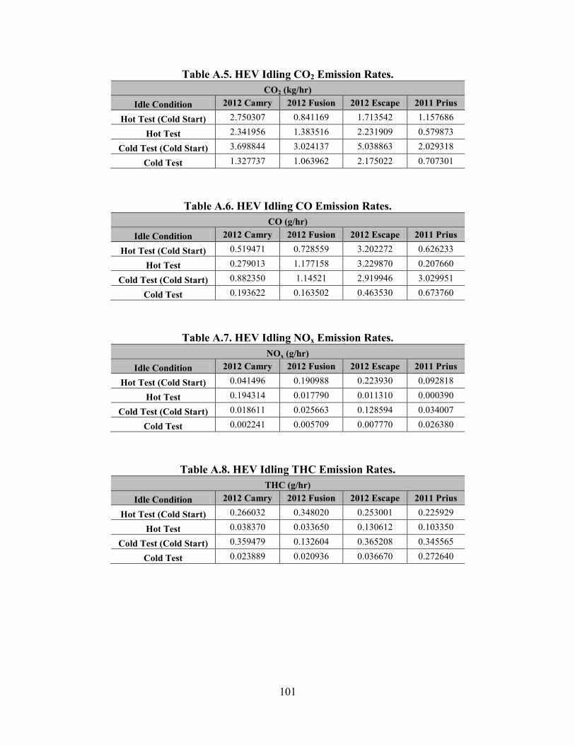
101
Table A.5. HEV Idling CO2 Emission Rates. CO2 (kg/hr)
Idle Condition 2012 Camry 2012 Fusion 2012 Escape 2011 Prius
Hot Test (Cold Start) 2.750307 0.841169 1.713542 1.157686
Hot Test 2.341956 1.383516 2.231909 0.579873
Cold Test (Cold Start) 3.698844 3.024137 5.038863 2.029318
Cold Test 1.327737 1.063962 2.175022 0.707301
Table A.6. HEV Idling CO Emission Rates. CO (g/hr)
Idle Condition 2012 Camry 2012 Fusion 2012 Escape 2011 Prius
Hot Test (Cold Start) 0.519471 0.728559 3.202272 0.626233
Hot Test 0.279013 1.177158 3.229870 0.207660
Cold Test (Cold Start) 0.882350 1.14521 2.919946 3.029951
Cold Test 0.193622 0.163502 0.463530 0.673760
Table A.7. HEV Idling NOx Emission Rates. NOx (g/hr)
Idle Condition 2012 Camry 2012 Fusion 2012 Escape 2011 Prius
Hot Test (Cold Start) 0.041496 0.190988 0.223930 0.092818
Hot Test 0.194314 0.017790 0.011310 0.000390
Cold Test (Cold Start) 0.018611 0.025663 0.128594 0.034007
Cold Test 0.002241 0.005709 0.007770 0.026380
Table A.8. HEV Idling THC Emission Rates. THC (g/hr)
Idle Condition 2012 Camry 2012 Fusion 2012 Escape 2011 Prius
Hot Test (Cold Start) 0.266032 0.348020 0.253001 0.225929
Hot Test 0.038370 0.033650 0.130612 0.103350
Cold Test (Cold Start) 0.359479 0.132604 0.365208 0.345565
Cold Test 0.023889 0.020936 0.036670 0.272640
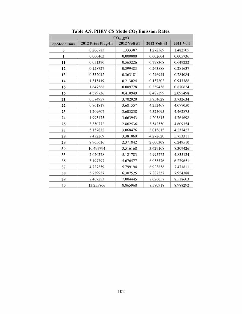
102
Table A.9. PHEV CS Mode CO2 Emission Rates. CO2 (g/s)
opMode Bins 2012 Prius Plug-In 2012 Volt #1 2012 Volt #2 2011 Volt
0 0.206783 1.333387 1.272569 1.482505 1 0.000463 0.000000 0.002604 0.005736
11 0.051390 0.563226 0.798368 0.649222 12 0.128727 0.399483 0.263888 0.281637 13 0.532042 0.363181 0.246944 0.784084 14 1.315419 0.213024 0.137802 0.943388 15 1.647568 0.009778 0.339438 0.870624 16 4.579736 0.410949 0.487599 2.095498 21 0.584957 3.702920 3.954628 3.732634 22 0.701817 3.681557 4.252467 4.077050 23 1.209607 3.603238 4.325095 4.462875 24 1.993175 3.663943 4.203815 4.761698 25 3.350772 2.862536 3.542550 4.609354 27 5.157832 3.068476 3.015615 4.237427 28 7.482269 3.381069 4.272620 5.753311 29 8.905616 2.371842 2.600308 6.249510 30 10.499794 3.516168 3.629108 8.309426 33 2.020278 5.121783 4.995272 4.835124 35 3.197797 5.676577 6.033376 6.279651 37 4.727359 5.799194 6.923858 7.471811 38 5.739957 6.307525 7.887537 7.954388 39 7.407253 7.004445 8.026057 8.518603 40 13.255866 8.865968 8.580918 8.988292

103
Table A.10. PHEV CS Mode CO Emission Rates. CO (g/s)
opMode Bins 2012 Prius Plug-In 2012 Volt #1 2012 Volt #2 2011 Volt
0 0.000317 0.063584 0.046440 0.070734 1 0.000003 0.000000 0.000008 0.000083
11 0.000131 0.001452 0.001608 0.002472 12 0.000275 0.002750 0.000501 0.001566 13 0.000513 0.004303 0.000429 0.002904 14 0.000880 0.001293 0.000186 0.003119 15 0.001156 0.003585 0.000496 0.004918 16 0.006190 0.012915 0.001557 0.006303 21 0.000366 0.123586 0.025677 0.062198 22 0.000307 0.091880 0.013095 0.065597 23 0.000661 0.116399 0.015739 0.062491 24 0.001131 0.075597 0.011150 0.074826 25 0.001101 0.024308 0.012157 0.034323 27 0.003562 0.021143 0.015407 0.028796 28 0.006373 0.103817 0.035974 0.032176 29 0.008567 0.042188 0.018251 0.129693 30 0.006362 0.189774 0.039630 0.113369 33 0.000816 0.280725 0.124609 0.154771 35 0.001334 0.287252 0.106790 0.135706 37 0.002700 0.308050 0.214637 0.259250 38 0.004173 0.473494 0.348864 0.338701 39 0.003116 0.747390 0.763204 0.485535 40 0.004793 1.036054 0.980230 0.839810

104
Table A.11. PHEV CS Mode NOx Emission Rates. NOx (g/s)
opMode Bins 2012 Prius Plug-In 2012 Volt #1 2012 Volt #2 2011 Volt
0 0.000011 0.000011 0.000151 0.000099 1 0.000000 0.000000 0.000000 0.000000
11 0.000000 0.000003 0.000026 0.000038 12 0.000006 0.000002 0.000027 0.000046 13 0.000019 0.000002 0.000020 0.000038 14 0.000034 0.000001 0.000007 0.000169 15 0.000074 0.000000 0.000011 0.000095 16 0.000693 0.000006 0.000035 0.000293 21 0.000013 0.000051 0.000269 0.000190 22 0.000032 0.000027 0.000130 0.000209 23 0.000018 0.000027 0.000200 0.000208 24 0.000017 0.000026 0.000145 0.000237 25 0.000093 0.000029 0.000126 0.000216 27 0.000222 0.000044 0.000365 0.000207 28 0.000208 0.000035 0.000421 0.000607 29 0.000504 0.000040 0.000515 0.000981 30 0.001831 0.000387 0.000655 0.001054 33 0.000075 0.000024 0.000220 0.000230 35 0.000030 0.000015 0.000202 0.000281 37 0.000076 0.000016 0.000280 0.000374 38 0.000119 0.000011 0.000410 0.000424 39 0.000068 0.000010 0.000314 0.000431 40 0.002975 0.000087 0.000519 0.000451

105
Table A.12. PHEV CS Mode THC Emission Rates. THC (g/s)
opMode Bins 2012 Prius Plug-In 2012 Volt #1 2012 Volt #2 2011 Volt
0 0.000008 0.000656 0.000553 0.000251 1 0.000000 0.000000 0.000005 0.000004
11 0.000000 0.000918 0.000074 0.000142 12 0.000002 0.001030 0.000187 0.000169 13 0.000006 0.001296 0.000381 0.000156 14 0.000009 0.000613 0.000066 0.000166 15 0.000004 0.000001 0.000002 0.000098 16 0.000067 0.000416 0.000004 0.000199 21 0.000003 0.000343 0.000727 0.000079 22 0.000007 0.000962 0.000089 0.000070 23 0.000006 0.000570 0.000207 0.000078 24 0.000006 0.000373 0.000254 0.000097 25 0.000034 0.000179 0.000860 0.000110 27 0.000029 0.000269 0.001104 0.000099 28 0.000052 0.000689 0.000024 0.000118 29 0.000121 0.000158 0.000116 0.000158 30 0.000274 0.002693 0.000714 0.000175 33 0.000049 0.000861 0.000170 0.000228 35 0.000041 0.001153 0.000273 0.000318 37 0.000058 0.001524 0.001544 0.000800 38 0.000067 0.002033 0.002205 0.001031 39 0.000099 0.003586 0.000988 0.000680 40 0.000468 0.004461 0.001716 0.000684

106
Table A.13. PHEV CS Mode Idling CO2 Emission Rates. CO2 (g/hr)
Idle Condition 2012 Prius Plug-In 2012 Volt #1 2012 Volt #2 2011 Volt
Hot Test (Cold Start) 0.304364 1.304041 2.581410 2.408431
Hot Test (Auto) 0.650506 1.755424 2.320106 3.077833
Cold Test (Cold Start) 1.662147 2.164913 2.363869 1.786422
Cold Test (Auto) 0.679624 1.420467 1.423375 1.741813
Table A.14. PHEV CS Mode Idling CO Emission Rates. CO (g/hr)
Idle Condition 2012 Prius Plug-In 2012 Volt #1 2012 Volt #2 2011 Volt
Hot Test (Cold Start) 0.132666 5.104767 4.387454 5.836191
Hot Test 0.122120 0.661294 1.324737 1.801881
Cold Test (Cold Start) 7.955499 6.151218 1.881553 1.688279
Cold Test 0.167451 0.690750 1.180267 2.403380
Table A.15. PHEV CS Mode Idling NOx Emission Rates. NOx (g/hr)
Idle Condition 2012 Prius Plug-In 2012 Volt #1 2012 Volt #2 2011 Volt
Hot Test (Cold Start) 0.001866 0.004526 0.128984 0.127490
Hot Test 0.004040 0.001549 0.098122 0.023907
Cold Test (Cold Start) 0.000000 0.060000 0.009477 0.126928
Cold Test 0.000000 0.000000 0.000000 0.015211
Table A.16. PHEV CS Mode Idling THC Emission Rates. THC (g/hr)
Idle Condition 2012 Prius Plug-In 2012 Volt #1 2012 Volt #2 2011 Volt
Hot Test (Cold Start) 0.087288 0.176099 0.471595 0.629596
Hot Test 0.082800 0.058742 0.006052 0.004781
Cold Test (Cold Start) 0.198780 0.386509 0.246265 0.372259
Cold Test 0.027565 0.022363 0.016300 0.059179

107
Table A.17. PHEV CD Mode Electricity Consumption Rates. Electricity (kWh/s)
opMode Bins 2012 Prius Plug-In 2012 Volt #1 2012 Volt #2 2011 Volt
0 0.000000 0.000000 0.000000 0.000000 1 0.000000 0.000387 0.000291 0.000404
11 0.000000 0.000000 0.000000 0.000000 12 0.005893 0.000768 0.001434 0.002006 13 0.002506 0.002916 0.003986 0.005413 14 0.006171 0.004216 0.006050 0.007157 15 0.008125 0.004399 0.007689 0.009175 16 0.014848 0.010441 0.014138 0.015584 21 0.000000 0.000000 0.000000 0.000000 22 0.001192 0.001411 0.001422 0.001276 23 0.003003 0.002633 0.002892 0.003032 24 0.006415 0.003760 0.004727 0.004420 25 0.009397 0.005407 0.007426 0.007315 27 0.015131 0.008010 0.009565 0.010164 28 0.018300 0.012266 0.016542 0.014094 29 N/A 0.016352 0.021783 0.020891 30 N/A 0.026611 0.029266 0.028739 33 0.004135 0.002436 0.001029 0.001286 35 0.007575 0.005580 0.006016 0.006123 37 0.011144 0.008210 0.008437 0.009401 38 N/A 0.011279 0.012260 0.012794 39 N/A 0.013207 0.018364 0.021680 40 N/A 0.027728 0.029557 0.031663
Note: N/A means the vehicle was never operated in CD mode in that operating mode bin. The various “0” values mean during those operating mode bins, the vehicle used regenerative braking to generate electricity and therefore did not consume electricity.

108
Table A.18. PHEV CD Mode CO2 Emission Rates. CO2 (g/s)
opMode Bins 2012 Prius Plug-In 2012 Volt #1 2012 Volt #2 2011 Volt
0 0.000000 0.000000 0.000000 0.000000 1 0.000000 0.207754 0.156194 0.216679
11 0.000000 0.000000 0.000000 0.000000 12 3.159255 0.411675 0.769092 1.075517 13 1.343845 1.563611 2.136822 2.902338 14 3.308439 2.260376 3.243816 3.837275 15 4.355952 2.358362 4.122465 4.919020 16 7.960964 5.597711 7.579839 8.355127 21 0.000000 0.000000 0.000000 0.000000 22 0.639236 0.756325 0.762330 0.684259 23 1.610197 1.411562 1.550368 1.625619 24 3.439250 2.016105 2.534290 2.370010 25 5.038141 2.898726 3.981328 3.921879 27 8.112662 4.294286 5.128038 5.449595 28 9.811344 6.576528 8.868896 7.556239 29 N/A 8.767152 11.678796 11.200860 30 N/A 14.267322 15.690865 15.408516 33 2.217163 1.305857 0.551919 0.689385 35 4.061447 2.991931 3.225542 3.282891 37 5.974637 4.401708 4.523632 5.040133 38 N/A 6.047415 6.572914 6.859494 39 N/A 7.080964 9.845594 11.623649 40 N/A 14.866478 15.846867 16.976081
Note: N/A means the vehicle was never operated in CD mode in that operating mode bin. The various “0” values mean during those operating mode bins, the vehicle used regenerative braking to generate electricity and therefore did not consume electricity.

109
Table A.19. PHEV CD Mode NOx Emission Rates. NOx (g/s)
opMode Bins 2012 Prius Plug-In 2012 Volt #1 2012 Volt #2 2011 Volt
0 0.000000 0.000000 0.000000 0.000000 1 0.000000 0.126551 0.095144 0.131987
11 0.000000 0.000000 0.000000 0.000000 12 1.924419 0.250767 0.468483 0.655137 13 0.818586 0.952454 1.301617 1.767922 14 2.015293 1.376879 1.975929 2.337426 15 2.653372 1.436566 2.511146 2.996358 16 4.849318 3.409773 4.617161 5.089417 21 0.000000 0.000000 0.000000 0.000000 22 0.389383 0.460706 0.464363 0.416807 23 0.980831 0.859835 0.944387 0.990225 24 2.094975 1.228084 1.543730 1.443661 25 3.068918 1.765721 2.425175 2.388962 27 4.941723 2.615809 3.123678 3.319551 28 5.976453 4.006007 5.402373 4.602785 29 N/A 5.340397 7.113987 6.822859 30 N/A 8.690754 9.557887 9.385898 33 1.350556 0.795446 0.336194 0.419930 35 2.473978 1.822496 1.964797 1.999731 37 3.639373 2.681244 2.755512 3.070132 38 N/A 3.683705 4.003805 4.178372 39 N/A 4.313278 5.997316 7.080395 40 N/A 9.055722 9.652914 10.340760
Note: N/A means the vehicle was never operated in CD mode in that operating mode bin. The various “0” values mean during those operating mode bins, the vehicle used regenerative braking to generate electricity and therefore did not consume electricity.

110
Table A.20. PHEV CD Mode Electricity Consumption Rates. Electricity (kWh)
Idle Condition 2012 Prius Plug-In 2012 Volt #1 2012 Volt #2 2011 Volt
Hot Test (Cold Start) 1.84 0.69 1.46 1.86
Hot Test 0.76 0.77 0.99 1.35
Cold Test (Cold Start) N/A 1.98 4.73 4.66
Cold Test N/A 2.03 1.84 2.89
Table A.21. PHEV CD Mode Idling CO2 Emission Rates. CO2 (kg/hr)
Idle Condition 2012 Prius Plug-In 2012 Volt #1 2012 Volt #2 2011 Volt
Hot Test (Cold Start) 0.990855 0.370369 0.782773 0.997231 Hot Test (Min) 0.409016 0.416371 0.530784 0.723797
Cold Test (Cold Start) N/A 1.063177 2.535971 2.498441 Cold Test N/A 1.092487 0.986508 1.549462
Table A.22. PHEV CD Mode Idling NOx Emission Rates. NOx (g/hr)
Idle Condition 2012 Prius Plug-In 2012 Volt #1 2012 Volt #2 2011 Volt
Hot Test (Cold Start) 0.603567 0.225605 0.476816 0.607451 Hot Test 0.249147 0.253627 0.323321 0.440892
Cold Test (Cold Start) N/A 0.647621 1.544754 1.521893 Cold Test N/A 0.665474 0.600919 0.943835
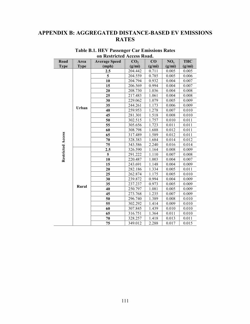
111
APPENDIX B: AGGREGATED DISTANCE-BASED EV EMISSIONS RATES
Table B.1. HEV Passenger Car Emissions Rates on Restricted Access Road.
Road Type
Area Type
Average Speed (mph)
CO2 (g/mi)
CO (g/mi)
NOx (g/mi)
THC (g/mi)
Res
tric
ted
Acc
ess
Urban
2.5 204.442 0.711 0.005 0.005 5 204.559 0.785 0.005 0.006
10 204.794 0.932 0.004 0.007 15 206.569 0.994 0.004 0.007 20 208.730 1.036 0.004 0.008 25 217.483 1.061 0.004 0.008 30 229.062 1.079 0.005 0.009 35 244.261 1.173 0.006 0.009 40 259.953 1.278 0.007 0.010 45 281.301 1.518 0.008 0.010 50 302.515 1.757 0.010 0.011 55 305.656 1.723 0.011 0.011 60 308.798 1.688 0.012 0.011 65 317.489 1.589 0.012 0.011 70 328.383 1.684 0.014 0.012 75 343.586 2.240 0.016 0.014
Rural
2.5 326.590 1.164 0.008 0.009 5 291.222 1.110 0.007 0.008
10 220.487 1.003 0.004 0.007 15 243.691 1.148 0.004 0.009 20 282.186 1.334 0.005 0.011 25 262.874 1.175 0.005 0.010 30 239.872 0.994 0.004 0.009 35 237.237 0.973 0.005 0.009 40 250.797 1.081 0.005 0.009 45 273.768 1.235 0.007 0.009 50 296.740 1.389 0.008 0.010 55 302.292 1.414 0.009 0.010 60 307.845 1.439 0.010 0.010 65 316.751 1.364 0.011 0.010 70 328.257 1.418 0.013 0.011 75 349.012 2.288 0.017 0.015

112
Table B.2. HEV Passenger Car Emissions Rates on Unrestricted Access Road.
Road Type
Area Type
Average Speed (mph)
CO2 (g/mi)
CO (g/mi)
NOx (g/mi)
THC (g/mi)
Unr
estr
icte
d A
cces
s
Urban
2.5 242.011 0.850 0.006 0.007 5 202.269 0.960 0.004 0.006
10 216.320 1.108 0.003 0.008 15 231.785 1.205 0.003 0.009 20 239.726 1.184 0.004 0.009 25 233.257 1.053 0.004 0.009 30 242.303 1.077 0.005 0.009 35 259.819 1.220 0.005 0.010 40 279.300 1.428 0.007 0.011 45 300.963 1.829 0.009 0.012 50 317.857 2.134 0.012 0.013 55 309.708 1.932 0.011 0.012 60 301.560 1.730 0.011 0.011 65 307.732 1.580 0.012 0.011 70 328.383 1.684 0.014 0.012 75 343.586 2.240 0.016 0.014
Rural
2.5 279.132 1.019 0.007 0.008 5 231.845 1.108 0.004 0.007
10 208.993 1.066 0.003 0.007 15 273.344 1.368 0.004 0.011 20 258.783 1.226 0.004 0.010 25 242.117 1.102 0.004 0.009 30 266.986 1.342 0.005 0.011 35 276.536 1.309 0.005 0.011 40 283.677 1.295 0.007 0.010 45 318.736 2.020 0.011 0.013 50 352.683 2.721 0.014 0.015 55 332.169 2.203 0.013 0.013 60 311.656 1.685 0.011 0.011 65 309.198 1.360 0.011 0.010 70 328.257 1.418 0.013 0.011 75 349.012 2.288 0.017 0.015

113
Table B.3. HEV Passenger Truck Emissions Rates on Restricted Access Road.
Road Type
Area Type
Average Speed (mph)
CO2 (g/mi)
CO (g/mi)
NOx (g/mi)
THC (g/mi)
Res
tric
ted
Acc
ess
Urban
2.5 238.395 1.780 0.012 0.019 5 234.545 2.113 0.014 0.018
10 226.847 2.779 0.017 0.017 15 233.426 2.774 0.018 0.015 20 245.022 2.532 0.018 0.013 25 267.122 2.861 0.021 0.013 30 293.724 3.434 0.023 0.014 35 323.103 5.784 0.031 0.025 40 352.861 8.376 0.038 0.036 45 392.117 12.549 0.050 0.053 50 431.244 16.741 0.062 0.070 55 444.714 18.668 0.068 0.076 60 458.183 20.595 0.074 0.081 65 465.653 22.254 0.083 0.083 70 476.444 26.850 0.096 0.096 75 495.876 38.343 0.119 0.138
Rural
2.5 308.428 2.923 0.014 0.031 5 293.682 2.803 0.016 0.026
10 264.189 2.562 0.018 0.017 15 291.755 3.441 0.024 0.019 20 328.610 4.503 0.029 0.022 25 319.036 3.777 0.027 0.017 30 306.499 2.936 0.023 0.013 35 316.159 4.144 0.027 0.018 40 343.570 6.979 0.035 0.031 45 386.123 10.718 0.046 0.046 50 428.677 14.458 0.057 0.062 55 443.042 16.839 0.065 0.069 60 457.406 19.219 0.073 0.075 65 465.674 20.815 0.082 0.077 70 473.176 23.703 0.093 0.084 75 484.660 34.410 0.116 0.125

114
Table B.4. HEV Passenger Truck Emissions Rates on Unrestricted Access Road.
Road Type
Area Type
Average Speed (mph)
CO2 (g/mi)
CO (g/mi)
NOx (g/mi)
THC (g/mi)
Unr
estr
icte
d A
cces
s
Urban
2.5 267.718 2.146 0.013 0.022 5 208.911 1.954 0.013 0.017
10 212.770 1.734 0.015 0.013 15 238.806 1.828 0.017 0.011 20 273.931 2.037 0.020 0.010 25 290.710 2.031 0.020 0.009 30 309.366 2.995 0.024 0.012 35 338.317 5.455 0.031 0.023 40 370.536 8.637 0.041 0.036 45 408.802 13.848 0.055 0.057 50 445.218 18.527 0.067 0.075 55 471.917 20.421 0.076 0.082 60 474.735 21.621 0.082 0.084 65 472.311 22.669 0.086 0.084 70 476.444 26.850 0.096 0.096 75 495.876 38.343 0.119 0.138
Rural
2.5 287.244 1.867 0.014 0.020 5 220.472 1.753 0.014 0.015
10 234.830 1.859 0.016 0.014 15 295.614 2.294 0.021 0.013 20 288.048 2.209 0.021 0.011 25 300.195 1.932 0.020 0.008 30 324.042 2.942 0.026 0.011 35 349.151 5.472 0.033 0.023 40 381.567 9.841 0.044 0.042 45 440.128 17.841 0.067 0.070 50 484.378 23.560 0.084 0.091 55 477.890 21.188 0.079 0.085 60 475.063 21.140 0.081 0.081 65 473.039 21.602 0.086 0.079 70 473.176 23.703 0.093 0.084 75 484.660 34.410 0.116 0.125

115
Table B.5. PHEV Passenger Car Emissions Rates on Restricted Road.
Road Type
Area Type
Average Speed (mph)
CO2 (g/mi)
CO (g/mi)
NOx (g/mi)
THC (g/mi)
Res
tric
ted
Urban
2.5 240.275 4.675 0.013 0.140 5 228.370 4.145 0.013 0.121
10 204.560 3.086 0.011 0.081 15 221.644 3.128 0.011 0.060 20 250.263 3.480 0.011 0.044 25 270.091 3.727 0.011 0.036 30 288.245 3.954 0.011 0.029 35 290.224 4.550 0.011 0.028 40 290.798 5.178 0.011 0.027 45 297.794 6.137 0.010 0.029 50 304.790 7.096 0.010 0.030 55 308.107 7.911 0.010 0.032 60 311.271 8.720 0.009 0.035 65 309.671 9.537 0.010 0.038 70 309.342 10.546 0.011 0.041 75 312.906 12.103 0.013 0.044
Rural
2.5 238.371 4.590 0.013 0.137 5 228.370 4.145 0.013 0.121
10 204.560 3.086 0.011 0.081 15 281.560 3.934 0.013 0.058 20 309.250 4.481 0.013 0.046 25 296.889 4.595 0.012 0.039 30 284.529 4.709 0.010 0.031 35 279.737 4.170 0.010 0.026 40 276.242 3.673 0.010 0.022 45 292.272 5.210 0.010 0.026 50 308.302 6.746 0.009 0.029 55 311.954 7.528 0.009 0.031 60 313.154 8.167 0.008 0.033 65 309.753 8.814 0.009 0.037 70 307.605 9.644 0.010 0.040 75 319.877 12.564 0.013 0.046

116
Table B.6. PHEV Passenger Car Emissions Rates on Unrestricted Access Road.
Road Type
Area Type
Average Speed (mph)
CO2 (g/mi)
CO (g/mi)
NOx (g/mi)
THC (g/mi)
Unr
estr
icte
d A
cces
s
Urban
2.5 301.066 2.735 0.017 0.237 5 220.084 3.099 0.012 0.120
10 210.319 3.013 0.011 0.072 15 232.009 3.176 0.011 0.051 20 270.601 3.562 0.012 0.039 25 301.287 3.819 0.012 0.031 30 301.849 3.727 0.012 0.027 35 298.481 4.029 0.012 0.026 40 295.644 4.569 0.012 0.026 45 298.134 5.907 0.011 0.028 50 301.563 7.044 0.010 0.031 55 306.400 7.882 0.010 0.033 60 311.238 8.719 0.009 0.035 65 309.671 9.537 0.010 0.038 70 309.342 10.546 0.011 0.041 75 312.906 12.103 0.013 0.044
Rural
2.5 313.526 2.865 0.018 0.246 5 220.606 3.107 0.012 0.120
10 233.557 3.321 0.012 0.075 15 232.903 3.188 0.011 0.051 20 292.797 3.823 0.012 0.039 25 301.619 3.822 0.012 0.031 30 314.842 3.923 0.012 0.027 35 304.047 4.146 0.012 0.026 40 295.644 4.569 0.012 0.026 45 298.134 5.907 0.011 0.028 50 301.913 6.952 0.010 0.030 55 307.625 7.559 0.009 0.032 60 313.154 8.167 0.008 0.033 65 309.753 8.814 0.009 0.037 70 307.605 9.644 0.010 0.040 75 319.877 12.564 0.013 0.046

117
APPENDIX C: PILOT APPLICATION RESULTS
Table C.1. Harris County Emissions Summary for 2014 Scenarios. Pollutant Vehicle Type Base Case 2014 (ton/day) EV 2014 (ton/day)
CO2
Passenger Car 30,213.78 29,890.54
Passenger Truck 8048.70 8037.40
Fleet Total 52,829.76 52,495.23
CO
Passenger Car 191.76 191.58
Passenger Truck 80.22 80.96
Fleet Total 329.19 329.75
NOx
Passenger Car 19.02 18.27
Passenger Truck 10.48 10.43
Fleet Total 65.58 64.78
THC
Passenger Car 3.63 3.55
Passenger Truck 2.30 2.29
Fleet Total 9.82 9.73

118
Table C.2. Harris County Emissions Summary for 2026 Scenarios.
Pollutant Vehicle Type Base Case
2026 (ton/day)
Low Oil Price 2026
(ton/day)
Medium Oil Price 2026
(ton/day)
High Oil Price 2026
(ton/day)
Extended Incentive 2026
(ton/day)
CO2
Passenger Car 29,859.74 28,674.57 28,484.21 28,136.42 27,959.78
Passenger Truck 7477.30 7276.51 7244.85 7194.90 7127.88
Fleet Total 54,019.82 52,633.87 52,411.85 52,014.11 51,770.45
CO
Passenger Car 147.26 159.92 161.11 163.61 158.67
Passenger Truck 50.63 64.27 65.75 68.45 64.26
Fleet Total 239.22 265.53 268.19 273.39 264.26
NOx
Passenger Car 6.13 5.51 5.42 5.25 5.33
Passenger Truck 4.41 4.12 4.08 4.02 4.02
Fleet Total 25.38 24.47 24.34 24.11 24.19
THC
Passenger Car 1.59 1.69 1.70 1.71 1.67
Passenger Truck 0.94 0.94 0.94 0.94 0.93
Fleet Total 4.60 4.70 4.71 4.72 4.66