ABSTRACT Title of dissertation: ESSAYS ON INEQUALITY ...

ABSTRACT

Title of dissertation: ESSAYS ON INEQUALITY, SOCIAL MOBILITY

AND REDISTRIBUTIVE PREFERENCES

IN TRANSITION ECONOMIES

Alexandru Cojocaru, Doctor of Philosophy, 2012

Dissertation directed by: Professor Carol Graham

School of Public Policy

In this dissertation I rely on attitudinal and subjective well-being data from Transition

Economies to examine several aspects of the relationship between inequality, social mobility and

citizens’ preferences for government involvement in redistributive policies. In the second chapter I

suggest that if aversion to inequality is driven by social mobility considerations or by differences in

status between self and relevant others, then aggregate statistical indices of inequality will be unable

to capture in a meaningful way changes in status implicit in inequality dynamics. An alternative

test of inequality aversion that derives from the experimental literature is adopted, that is better

able to capture status driven aversion to inequality. The third chapter investigates empirically the

link between the prospects of upward mobility (POUM) and preferences for redistribution. The

POUM hypothesis is tested while directly accounting for other factors affecting preferences for

redistribution such as risk aversion, beliefs regarding effort and luck as determinants of success,

past economic mobility, or religious preferences. The chapter then looks at what shapes individuals’

beliefs vis-a-vis future economic mobility. In particular, I examine the role of perceived inequality

of opportunity, conceptualised in the spirit of John Rawls. The fourth chapter is concerned with

the body of literature that suggests that relative status is an important determinant of well-being

by looking at the effect of one’s income relative to some reference group on self-reported life

satisfaction. In most of these studies the data come from developed countries, while the reference

group of the individual is unknown, and thus imposed by the researcher. This essay looks instead

at self-reported relative deprivation based on data from six countries from different parts of Eastern

Europe and Former Soviet Union and which are at different levels of economic development. The

relative salience of several reference groups is examined. Given the cross-sectional nature of the

data, an instrumental variable strategy is employed to establish a causal link between relative

deprivation and the level of satisfaction with the household’s standard of living.

ESSAYS ON INEQUALITY, SOCIAL MOBILITYAND REDISTRIBUTIVE PREFERENCES IN TRANSITION ECONOMIES

by

Alexandru Cojocaru

Dissertation submitted to the Faculty of the Graduate School of theUniversity of Maryland, College Park in partial fulfillment

of the requirements for the degree ofDoctor of Philosophy

2012

Advisory Committee:Professor Carol Graham, ChairProfessor Branko MilanovicProfessor Madiha AfzalProfessor Peter MurrellProfessor Andrew Clark

c© Copyright byAlexandru Cojocaru

2012

Dedication

To my family

ii

Acknowledgments

I am grateful to my dissertation adviser, Carol Graham, for encouraging my interest in

subjective well-being and relative status research, for many discussions and for reading multiple

drafts of the essays that comprise this dissertation. I would also like to thank my committee

members – Madiha Afzal, Andrew Clark, Branko Milanovic and Peter Murrell – for insightful

comments on earlier versions of these essays; their suggestions helped me considerably improve

both the conceptualisation and the exposition.

Over the years, this work has also benefited from conversations with Stacy Kosko, Bob

Rijkers, Francisco Ferreira, Caterina Ruggeri Laderchi, Mame Fatou Diagne, Roy van der Weide,

Jorge Holzer, Randi Hjalmarsson and Kabir Malik, as well as the participants of the AISSEC

Workshop “Comparing Inequalities” in Assisi, the “Health, Happiness, Inequality” conference in

Darmstadt, the Fourth Meeting of the Society for the Study of Economic Inequality (ECINEQ)

in Catania, and the UNU-WIDER Conference on Poverty and Behavioural Economics in Helsinki.

None but me are responsible for any remaining errors.

I would also like to thank the Maryland School of Public Policy for providing me with

a supporting environment throughout the course of my doctoral studies and the departments of

Economics and of Agricultural and Resource Economics on whose resources I drew extensively.

Also, thanks to the European Bank for Reconstruction and Development for access to the data

used in chapters 2 and 3, and to the United Nations Development Programme for access to the

data used in chapter 4.

Last but not least, I would like to express my deep gratitude to my wife, Stacy Kosko, for

constant support, encouragement and understanding.

iii

Contents

1. Introduction . . . . . . . . . . . . . . . . . . . . . . . . . . . . . . . . . . . . . . . . . . . 1

2. Inequality and well-being: a non-experimental test of inequality aversion . . . . . . . . . 42.1 Introduction . . . . . . . . . . . . . . . . . . . . . . . . . . . . . . . . . . . . . . . . 42.2 Social evaluation, inequality aversion, and reference groups . . . . . . . . . . . . . 7

2.2.1 Existing literature . . . . . . . . . . . . . . . . . . . . . . . . . . . . . . . . 72.2.2 Proposed methodology . . . . . . . . . . . . . . . . . . . . . . . . . . . . . . 102.2.3 Relevant reference groups . . . . . . . . . . . . . . . . . . . . . . . . . . . . 152.2.4 Evaluative space and status observability . . . . . . . . . . . . . . . . . . . 182.2.5 Adaptation . . . . . . . . . . . . . . . . . . . . . . . . . . . . . . . . . . . . 192.2.6 Specifying a welfare metric . . . . . . . . . . . . . . . . . . . . . . . . . . . 21

2.3 Data . . . . . . . . . . . . . . . . . . . . . . . . . . . . . . . . . . . . . . . . . . . . 232.4 Empirical analysis of inequality aversion and well-being . . . . . . . . . . . . . . . 27

2.4.1 What is driving inequality aversion? . . . . . . . . . . . . . . . . . . . . . . 372.4.2 Implications for social welfare . . . . . . . . . . . . . . . . . . . . . . . . . . 432.4.3 Inequality aversion and support for redistribution . . . . . . . . . . . . . . . 44

2.5 Concluding remarks . . . . . . . . . . . . . . . . . . . . . . . . . . . . . . . . . . . 46

3. Prospects of upward mobility, inequality of opportunity and preferences for redistribution 493.1 Introduction . . . . . . . . . . . . . . . . . . . . . . . . . . . . . . . . . . . . . . . . 493.2 Empirical strategy . . . . . . . . . . . . . . . . . . . . . . . . . . . . . . . . . . . . 51

3.2.1 Data requirements and existing studies . . . . . . . . . . . . . . . . . . . . . 513.2.2 Empirical model . . . . . . . . . . . . . . . . . . . . . . . . . . . . . . . . . 55

3.3 Data description . . . . . . . . . . . . . . . . . . . . . . . . . . . . . . . . . . . . . 593.4 Main results and robustness checks . . . . . . . . . . . . . . . . . . . . . . . . . . . 64

3.4.1 Main results . . . . . . . . . . . . . . . . . . . . . . . . . . . . . . . . . . . . 643.4.2 Robustness analysis . . . . . . . . . . . . . . . . . . . . . . . . . . . . . . . 71

3.5 Inequality of opportunity and perceptions of upward mobility . . . . . . . . . . . . 733.5.1 Empirical strategy . . . . . . . . . . . . . . . . . . . . . . . . . . . . . . . . 773.5.2 Results . . . . . . . . . . . . . . . . . . . . . . . . . . . . . . . . . . . . . . 80


4. Does relative deprivation matter in developing countries? . . . . . . . . . . . . . . . . . 894.1 Introduction . . . . . . . . . . . . . . . . . . . . . . . . . . . . . . . . . . . . . . . . 894.2 Existing studies of relative status . . . . . . . . . . . . . . . . . . . . . . . . . . . . 91

4.2.1 Reference groups based on ’likeness’ . . . . . . . . . . . . . . . . . . . . . . 924.2.2 Reference groups based on geographic proximity . . . . . . . . . . . . . . . 944.2.3 Intermediate approaches . . . . . . . . . . . . . . . . . . . . . . . . . . . . . 954.2.4 Observed reference groups . . . . . . . . . . . . . . . . . . . . . . . . . . . . 97

4.3 Data and descriptive statistics . . . . . . . . . . . . . . . . . . . . . . . . . . . . . . 984.4 Empirical analysis . . . . . . . . . . . . . . . . . . . . . . . . . . . . . . . . . . . . 105

4.4.1 Salience of different reference groups . . . . . . . . . . . . . . . . . . . . . . 1054.4.2 More on local relative deprivation - IV results . . . . . . . . . . . . . . . . . 110


5. Overall conclusion . . . . . . . . . . . . . . . . . . . . . . . . . . . . . . . . . . . . . . . 119

Bibliography . . . . . . . . . . . . . . . . . . . . . . . . . . . . . . . . . . . . . . . . . . . . 121

iv

List of Tables

2.1 Summary statistics . . . . . . . . . . . . . . . . . . . . . . . . . . . . . . . . . . . 242.2 CEA level Gini index of inequality by country . . . . . . . . . . . . . . . . . . . . 262.3 Baseline FS model of inequality aversion, by region . . . . . . . . . . . . . . . . . . 312.4 Model with the Gini measure of inequality, by region . . . . . . . . . . . . . . . . . 342.5 Specification with reference group fixed effects . . . . . . . . . . . . . . . . . . . . . 352.6 Further robustness checks . . . . . . . . . . . . . . . . . . . . . . . . . . . . . . . . 362.7 Injustice vs laziness . . . . . . . . . . . . . . . . . . . . . . . . . . . . . . . . . . . . 382.8 Hard work vs political and criminal connections . . . . . . . . . . . . . . . . . . . . 392.9 Winners and losers of the transition process . . . . . . . . . . . . . . . . . . . . . . 412.10 Inequality aversion among young and old respodents . . . . . . . . . . . . . . . . . 422.11 Inequality and well-being across groups . . . . . . . . . . . . . . . . . . . . . . . . 442.12 Institutions and attitudes toward redistribution . . . . . . . . . . . . . . . . . . . . 46

3.1 Current and future welfare ladder placement . . . . . . . . . . . . . . . . . . . . . 613.2 Future mobility categories by country . . . . . . . . . . . . . . . . . . . . . . . . . 623.3 Summary statistics by region . . . . . . . . . . . . . . . . . . . . . . . . . . . . . . 633.4 POUM Hypothesis - Baseline . . . . . . . . . . . . . . . . . . . . . . . . . . . . . . 663.5 POUM Hypothesis: EU and non-EU countries . . . . . . . . . . . . . . . . . . . . 683.6 POUM Hypothesis - Alternative inequality preference . . . . . . . . . . . . . . . . 723.7 Falsification exercise - artificially low threshold . . . . . . . . . . . . . . . . . . . . 733.8 Importance of having connections . . . . . . . . . . . . . . . . . . . . . . . . . . . . 753.9 Inequality of opportunity . . . . . . . . . . . . . . . . . . . . . . . . . . . . . . . . 823.10 Differentiating by likelihood of using connections . . . . . . . . . . . . . . . . . . . 833.11 Inequality of opportunity and returns to education . . . . . . . . . . . . . . . . . . 853.12 Inequality of opportunity and redistributive preferences . . . . . . . . . . . . . . . 86

4.1 Satisfaction with standard of living by country . . . . . . . . . . . . . . . . . . . . 994.2 Asset index by satisfaction level . . . . . . . . . . . . . . . . . . . . . . . . . . . . . 1004.3 Relative deprivation for various reference groups . . . . . . . . . . . . . . . . . . . 1014.4 Relative status and household welfare (asset index) . . . . . . . . . . . . . . . . . 1024.5 Summary statistics by country . . . . . . . . . . . . . . . . . . . . . . . . . . . . . 1034.6 Relative status and satisfaction with living standards - different reference groups . 1074.7 Relative status and satisfaction with living standards - interactions . . . . . . . . . 1094.8 Relative status and satisfaction with living standards - OLS . . . . . . . . . . . . . 1124.9 Relative status and satisfaction with living standards - 2SLS . . . . . . . . . . . . 115

v

1 Introduction

“All societies are inegalitarian. But what is the relation between the

inequalities in a society and the feelings of acquiescence or resentment to

which they give rise?” (W.G. Runciman, 1972:3)

The countries of Eastern Europe and the Former Soviet Union have undergone a

vast transformation – economic, political, and social – over the course of the past

two decades. One of the important features of this transformation has been the con-

siderable increase in economic inequality in the region since the beginning of tran-

sition. Inequality is also perceived to be excessive by the citizens in post-Socialist

Europe – in a recent survey more than 70 percent of respondents either agreed or

strongly agreed that the gap between the rich and the poor in their countries should

be reduced. This dissertation tackles a number of issues pertaining to economic

inequality, social mobility, and preferences for redistributive policy in Transition

Economies. It focuses in particular on institutional factors like fairness and inequal-

ity of opportunity as key drivers of attitudes toward inequality and redistribution.

Yet, this dissertation is not merely concerned with the particular circumstances

of post-Socialist Europe. It aims to contribute to several strands of literature that

are not specific to any given geographic area. For instance, the first essay aims to

contribute to the small literature concerned with the general question of whether

preferences for fairness observed in laboratory experiments can be similarly found

among “regular people” and addresses some of the methodological challenges in-

1

volved in testing for aversion to inequality with observational data. The second

essay aims to contribute to the nascent literature on the measurement and impli-

cations of inequality of opportunity, and also to the broader literature concerned

with the link between redistributive preferences and institutional factors life beliefs

about the degree of fairness in the distribution of fortunes in society. The third

essay adds empirical evidence to the emerging literature on the importance of rel-

ative status for well-being, particularly in developing countries, where the evidence

remains sparse and the results – mixed. More generally, the dissertation relies on

attitudinal and subjective well-being data from household surveys and comments

on several methodological aspects pertaining to the use of such data to examine the

importance of inequality and relative status for well-being.

If there is a common thread that unites the three essays, it is that all three

are concerned with the importance of relative position within different reference

groups. The first essay focuses on one’s position vis-a-vis neighbours, and, to a

limited extent, one’s position relative to a salient point in the past (here the pre-

transition level of welfare). The second essay looks into the future and examines

the importance of expected future changes in the individual’s relative position in

society. The third essay examines the salience of a number of different reference

groups such as parents or grandparents, or local reference groups at different levels

of geographic aggregation. To a large extent, reference points – both inter-temporal

and inter-personal – are found to be salient for individuals’ assessments of well-being

and for their policy preferences.

A second common thread that spans two of the three essays is the emphasis on

2

institutional aspects of the transition process, and in particular, on the individual

beliefs about institutions (largely informal ones). Beliefs about the existence of

inequality of opportunity (in a Rawlsian sense), and about the importance of effort

and luck for success in society are found to influence the degree of tolerance for

economic inequality, preferences over redistributive policy, as well as expectations of

one’s ability to progress up the socio-economic ladder in the future. These findings

seem particularly relevant in light of the increasing concern in analytical and policy

debates with the extent and the implications of inequality of opportunity.

3

2 Inequality and well-being: a non-experimental test of inequalityaversion

2.1 Introduction

On October 15, 2011 Occupy protests that originated with the Occupy Wall

Street movement in New York were planned in over 80 countries and 950 cities

worldwide. These protests are perhaps the most vivid manifestation of the growing

global concern with equity and inequality, also reflected in China’s pledge to create

a “harmonious society”, or in the indicators underpinning European Union’s “social

inclusion agenda”, or in the recommendation of the Sarkozy Commission (on the

Measurement of Economic Performance and Social Progress) that “[q]uality-of-life

indicators in all the dimensions covered should assess inequalities in a comprehen-

sive way.” (Stiglitz, Sen and Fitoussi, 2009). This concern is driven in part by the

oftentimes sharp increase in the gap between the rich and the poor over the past two

decades in many OECD countries, in China, and in Eastern Europe. Yet, the map-

ping from a given statistical measure of inequality to preferences for redistribution,

or to individual (social) welfare, and the importance of tradeoffs between the size

of the pie and the inequality in its distribution will be influenced by the prevailing

degree of inequality aversion in society.1 The latter is the subject of this paper.

Some evidence of aversion to inequality can be inferred from the preferences

for equity that have been observed in tightly controlled lab experiments, where

individuals have been observed to have strong other-regarding preferences, to prefer

equitable outcomes, and to engage in cooperation (see Fehr and Schmidt 2006 for

1 In the case of social welfare, the normative degree of inequality aversion in the social welfare function will alsoplay a crucial role (Sen 1997 provides a detailed discussion).

4

a comprehensive review of the literature). These other-regarding preferences have

been observed in a number of different games, such as ultimatum games (Thaler,

1988; Camerer and Thaler, 1995), public goods games with punishments (Fehr and

Gachter, 1996), or gift exchange games (Fehr, Gachter, and Kirchsteiger, 1997), as

well as in other contexts.

This paper investigates, rather, the degree of inequality aversion based on

nationally representative household survey data. Evidence on this is more scarce

and generally looks at associations between inequality, usually measured in terms of

some statistical index like the Gini index, and subjective well-being using household

survey data (Tomes 1986; Clark 2003; Alesina et al. 2004; Senik 2004; Graham and

Felton 2006; Grosfeld and Senik 2010). A negative association between inequality

and well-being is viewed as indicative of inequality being a welfare-relevant consider-

ation in the population. The motivation behind this line of research stems from the

argument that aversion to inequality, by its nature, offers only a limited scope for

revealed choice analysis, but more progress could be made by analysing expressed

preferences. These studies reach mixed conclusions, inequality having either a posi-

tive, a negative, or no statistically discernible effect on individual well-being.

This paper suggests that if aversion to inequality is driven by social mobility

considerations or by differences in status between self and relevant others, then ag-

gregate statistical indices of inequality will be unable to capture in a meaningful way

changes in status implicit in inequality dynamics. An alternative test of inequality

aversion is adopted, that is better able to capture, I believe, status-driven aversion

to inequality. The test builds on the model of inequality aversion proposed in the

5

experimental literature by Fehr and Schmidt (1999), which is closely related to ear-

lier work on relative deprivation by Yitzhaki (1979). The proposed specification,

while intimately related to the Gini index, allows us to make progress in settings

where aggregate measures of inequality are less appealing.

Several findings emerge from this study. First, individuals are found to exhibit

aversion to inequality (in the sense of Fehr and Schmidt, 1999), and this result holds

across a number of specifications, and also across regional subsets of countries. The

Gini index, on the other hand, is unable to capture this negative effect of inequal-

ity on well-being. Second, inequality aversion does not appear to be intrinsic, but

rather stems from a sense of fairness, as captured by opinions vis-a-vis the main

determinants of success and economic need in society. As such, the findings are sug-

gestive of inequality of opportunity being the factor that is driving the individuals’

responses to economic inequality. Finally, perceiving inequality to be unfair is also

associated with calls for strong government involvement in redistributive policies.

Section 2.2 reviews existing findings on inequality and subjective well-being,

discusses the proposed methodology and addresses some of the difficulties of testing

for inequality aversion with large household survey data. Section 2.3 describes the

survey data employed in the empirical analysis. Section 2.4 presents the main find-

ings, discusses the driving forces behind inequality aversion, and considers implica-

tions for social welfare and support of redistributive policies. Section 2.5 concludes.

6

2.2 Social evaluation, inequality aversion, and reference groups

2.2.1 Existing literature

The primary aim of this paper is to test for inequality aversion using nationally-

representative survey data. In the existing literature there are two types of studies

that share this goal, at least to some degree. First, there are several recent stud-

ies that run experiments on populations that go beyond the usual student setting.

Guth, Schmidt and Sutter (2007) implement a three-person ultimatum game exper-

iment through the German weekly Die Zeit. A total of 5,132 readers took part in

the experiment, thus offering a much greater variation in socio-economic and demo-

graphic characteristics in the participant group. Their findings suggest considerable

parallelism between student and non-student behaviour, and thus help address the

common objection that university students who typically take part in laboratory ex-

periments are not representative of the general population. Bellemare et al. (2008)

implement an ultimatum game relying on a representative sample of the Dutch pop-

ulation drawn from the participants of the CentERpanel (2,000 households) and

find that young and highly educated subjects have lower aversion to inequality than

other groups.

Pirttila and Uusitalo (2010), using a representative survey of Finnish people,

present survey respondents with a ’leaky bucket’ experiment in which they probe the

respondent’s willingness to have the tax schedule adjusted to effect a transfer from

the top income decile to the bottom income decile. In addition, the authors also ask

respondents to compare the Finnish wage distribution to alternative distributions

with a higher mean and dispersion of income. While they find evidence in support

7

of inequality averse preferences, the results also suggest differences between the two

approaches - a large group of respondents who supported more narrow wage differ-

ences do not support costly progressive transfers.2 The authors also find inequality

aversion to be strongly associated with attitudes to increased tax progression, with

increased unemployment insurance and unemployment assistance benefits, and with

increased income support.

A somewhat larger, albeit still limited, literature looks at the association be-

tween individual well-being and statistical measures of income inequality. This

question is apart from the larger literature that examines whether relative status

concerns, such as those embodied in the relation of someone’s income to mean (or

median) reference group income, or in someone’s rank in the income distribution, are

relevant for individual well-being (Clark and Oswald 1996; McBride 2001; Ravallion

and Lokshin 2002; Blanchflower and Oswald 2004; Ferrer-i-Carbonell 2005; Luttmer

2005; Graham and Felton 2006; see also Clark et al. 2008 for a recent review of

the literature). The relevant question here is whether conditional on own income,

and conditional on relative income, the degree of inequality in the distribution of

incomes in a given group has an effect on individual well-being. Existing studies

that explore the relationship between inequality and welfare based on household

survey data generally model individual well-being – proxied by a measure of self-

reported happiness or life satisfaction – as a function of the Gini index or some other

composite inequality measure. As already noted, they arrive at mixed results.

Tomes (1986), using survey data from Canada, finds higher levels of inequality

2 The authors conclude that it is unclear why this is the case, but note that it is plausible that a smaller increase inthe underlying latent preference for equality increases may trigger willingness to support an equal wage distribution,compared with the increase necessary to trigger support for costly transfers.

8

(as measured by the income share of the poorest 40 percent of the population) to be

positively associated with life satisfaction among men, controlling for own income

and average income in the district of residence. Clark (2003) similarly finds, using

data from the British Household Panel Survey, that well-being is positively corre-

lated with reference group income inequality measured by either the Gini coefficient

or the 90th / 10th percentile ratio.

On the other hand, Alesina et al. (2004), relying on US GSS survey data from

1972-1997, and Eurobarometer data for 1975-1992, find that inequality (measured by

the Gini coefficient) has a negative effect on happiness, controlling for own income

and a number of socio-demographic characteristics, albeit the relationship is less

precisely estimated in the US sample. They also find a strong negative effect of

inequality on happiness among the poor and the political left in Europe, but not

in the United States. A negative association between inequality and subjective

evaluations of the economic situation is found in the Grosfeld and Senik (2010)

study on Poland, but only for the second half of the transition period (1997-2005),

whereas a positive association is found in the early years (1992-1996).

Graham and Felton (2006), relying on Latinobarometro data from 18 countries

in Latin America find country-level inequality measured by the Gini index to not

have a statistically significant effect on happiness. Senik (2004), relying on panel

data from the Russian Longitudinal Monitoring Survey, finds that neither national

level inequality (measured by either Gini or Stark indices), nor the regional or Pri-

mary Sampling Unit inequality, have a significant effect on reported life satisfaction

in Russia.

9

2.2.2 Proposed methodology

Imagine an increase in the Gini index of income inequality for a given group

from, say, G1 = 0.22 to G2 = 0.29. Assume further that the group in question is

the relevant reference group (more on this in Section 2.2.3.) and that the inequality

in the income space is the relevant dimension for well-being evaluation (see Section

2.2.4.). Should we expect this sizable increase in the Gini index to have an effect

on individual well-being? The answer to this question depends in part on whether

individuals are averse to inequality, and if so, on the nature of this aversion. If

aversion to inequality is based on its perception as a social evil (Alesina et al. 2004),

then higher inequality should reduce the (individual) well-being of all irrespective of

the underlying changes in the income distribution that precipitated the increase in

inequality, or of the individuals’ position in this income distribution. If, on the other

hand, aversion to inequality is driven by perceptions of social mobility, aggregate

national measures of inequality may be limited in their ability to capture the subtle

effects of inequality on prospects of social mobility (Graham and Felton, 2006).

Similarly, if inequality aversion is driven by status considerations that are

sensitive to the distribution of incomes in the group and not just the individual’s

position in the income distribution, then aggregate measures of income distribution

will provide little useful information on implicit changes in status. Returning to

the above increase in the Gini index, consider instead the income distribution A1 =

{100, 200, 300} that corresponds to G1and A2 = {100, 200, 400} that corresponds

to G2. For someone with the income equal to 100, for instance, the change in

relative standing embodied in the income gaps between her and others in A2 relative

10

to the initial distribution A1 is much more explicit. The relative standing of the

person whose income increases from 300 to 400 actually improves as inequality

increases. It seems plausible for these bilateral differences between group members to

be important factors determining well-being (if status considerations matter), even

if composite inequality indices generated by these are not, in themselves, meaningful

indicators of inequality of status.

These bilateral gaps form the basis of the relative deprivation measure pro-

posed by Yitzhaki (1979). Given a range of incomes (0, y∗), Yitzhaki defines the total

deprivation of someone with income yi is the sum inherent in all units of income the

person is deprived of, or incomes in the interval (yi, y∗):

D(yi) =

ˆ y∗

yi

(z − yi)f(z)dz =

ˆ y∗

yi

[1− F (z)]dz

where F (y) =´ y∗

0f(z)dz is the cumulative income distribution. This definition is a

formalisation of the concept of relative deprivation proposed by Runciman (1972).

Yitzhaki further shows that the degree of relative deprivation within a given group

is the product of the group’s mean income and its Gini index of inequality (G), such

that:

G =1

µ

ˆ y∗

0

D(z)f(z)dz

A number of studies establish a negative relationship between Yitzhaki’s mea-

sure of relative deprivation D(yi) and individual well-being (D’Ambrosio and Frick,

2007) or health outcomes within groups (Deaton, 2001; Eibner and Evans, 2005).

On the other hand, if one were to model individual well-being as a function of the

Gini index of inequality, this implicitly assumes that an individual’s utility (proxied

11

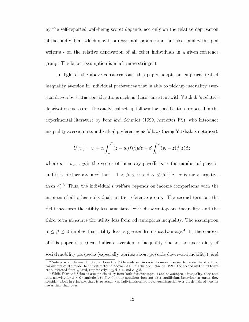
by the self-reported well-being score) depends not only on the relative deprivation

of that individual, which may be a reasonable assumption, but also - and with equal

weights - on the relative deprivation of all other individuals in a given reference

group. The latter assumption is much more stringent.

In light of the above considerations, this paper adopts an empirical test of

inequality aversion in individual preferences that is able to pick up inequality aver-

sion driven by status considerations such as those consistent with Yitzhaki’s relative

deprivation measure. The analytical set-up follows the specification proposed in the

experimental literature by Fehr and Schmidt (1999, hereafter FS), who introduce

inequality aversion into individual preferences as follows (using Yitzhaki’s notation):

U(yi) = yi + α

ˆ y∗

yi

(z − yi)f(z)dz + β

ˆ yi

0

(yi − z)f(z)dz

where y = y1, ..., ynis the vector of monetary payoffs, n is the number of players,

and it is further assumed that −1 < β ≤ 0 and α ≤ β (i.e. α is more negative

than β).3 Thus, the individual’s welfare depends on income comparisons with the

incomes of all other individuals in the reference group. The second term on the

right measures the utility loss associated with disadvantageous inequality, and the

third term measures the utility loss from advantageous inequality. The assumption

α ≤ β ≤ 0 implies that utility loss is greater from disadvantage.4 In the context

of this paper β < 0 can indicate aversion to inequality due to the uncertainty of

social mobility prospects (especially worries about possible downward mobility), and

3 Note a small change of notation from the FS formulation in order to make it easier to relate the structuralparameters of the model to the estimates in Section 2.4. In Fehr and Schmidt (1999) the second and third termsare subtracted from yi, and, respectively, 0 ≤ β < 1, and α ≥ β.

4 While Fehr and Schmidt assume disutility from both disadvantageous and advantageous inequality, they notethat allowing for β < 0 (equivalent to β > 0 in our notation) does not alter equilibrium behaviour in games theyconsider, albeit in principle, there is no reason why individuals cannot receive satisfaction over the domain of incomeslower than their own.

12

is also consistent with a preference for fairness with respect to the fortunes of the

poor.

Fehr and Schmidt (1999) show that many of the manifestations of fair and

cooperative behaviour in experimental studies, such as those observed in ultima-

tum games (Thaler, 1988; Camerer and Thaler, 1995), public goods games with

punishments (Fehr and Gachter, 1996), or gift exchange games (Fehr, Gachter, and

Kirchsteiger, 1997) can be explained if a fraction of subjects are inequality averse in

the above sense. In particular, they note that “[t]his utility function can rationalize

positive and negative actions towards other players. It is consistent with generosity

in dictator games and kind behavior of responders in trust games and gift exchange

games, and at the same time with the rejection of low offers in ultimatum games.

It can explain voluntary contributions in public good games and at the same time

costly punishments of free-riders.” (Fehr and Schmidt, 2006:640)

The advantage of using the FS specification is that the test for inequality

aversion is based on a self-regarding utility function that only considers the relative

deprivation of self, and not of all others in the reference group. It is also easily

observed that the FS specification is intimately related to Yitzhaki’s concept of

relative deprivation - the second term in the FS utility function is Yitzhaki’s measure

of relative deprivation D(yi), and the last term is a similar measure of normalised

aggregate income gap, but defined over incomes that are lower than the income

of the individual i. If we take Yitzhaki’s measure of relative satisfaction S(yi),

defined as: S(yi) =´ yi

0[1 − F (z)]dz, then the third term in the FS utility function

is´ yi

0(yi − z)f(z)dz = yi − S(yi). Thus, the FS utility function can be written as:

13

U(yi) = yi + αD(yi) + β(yi − S(yi))

As Yitzhaki’s notes further, D(yi) = µ − S(yi), and substituting into the above

equation, we can rewrite U(yi) equivalently as a function of own income, relative

income, and Yitzhaki’s relative deprivation, which is the specification used in section

2.4 of this paper:

U(yi) = yi + β(yi − µ) + (α + β)D(yi)

A further advantage of using the FS specification in a cross-sectional setting

stems from the fact that it allows us to investigate the relationship between inequal-

ity and well-being at the level of the individual. A regression of individual well-being

on a group inequality measure (e.g. Gini or Theil index) in a cross-section essen-

tially looks at the relationship between the mean well-being level in a group and the

group’s level of inequality because there is no within-group variation in the inequal-

ity measure. In principle, a negative association between life satisfaction and the

group inequality index would be consistent with the “social evil” hypothesis. There

is, however, an alternative explanation consistent with this negative relationship.

Consider v(yi), which is a concave function of individual income alone. The con-

cavity of the individual utility function will imply a negative relationship between

mean group life satisfaction and group inequality (Atkinson, 1970), even though at

the individual level inequality has no bearing on well-being.

The link between Yitzhaki’s relative deprivation and inequality is established

by Hey and Lambert (1980). In particular, fix mean group income µ and consider

14

two income distributions F1 and F2 where F1 Lorenz dominates F2, in other words

F2 is more unequal than F1. Hey and Lambert show that there will be more relative

deprivation at every level of income under F2. Since inequality averse preferences

imply that α+β < 0, higher inequality associated with F2 will have a negative effect

on individual well-being at every level of income. If, on the other hand, α + β = 0

and there is no aversion to inequality, higher relative deprivation under F2 would

have no effect on individual well-being (see also Deaton 2001).

A number of difficulties arise, however, when translating the FS specification

to an empirical setting based on large household survey data, namely: (i) whether

inequality in the general population could be expected to produce an evaluative re-

sponse that could be captured in an empirical test; (ii) what is the relevant group

over which the inequality measure is to be defined; and (iii) the nature of an ap-

propriate welfare metric. These issues are discussed in more detail below. It is

important to note, however, that these difficulties are not specific to the FS specifi-

cation alone; all of them apply equally to any study that proposes to examine the

relationship between individual life satisfaction and economic inequality defined for

some chosen reference group.

2.2.3 Relevant reference groups

In laboratory experiments, the relevant reference group is obvious in games

involving two subjects, and most theories of other-regarding preferences in n-person

games assume the remaining n−1 actors to form the relevant reference group (Fehr

and Schmidt, 2006). It is much less clear what the relevant reference groups are

in the general population for purposes of social comparisons, and there is little

15

consensus in the literature on this issue. In Veblen’s description of conspicuous

consumption behaviour the reference level of consumption was set by the affluent

(Veblen 1994, originally published in 1899). Duesenberry (1949) in formulating the

relative income hypothesis5 took the neighbours as the group against which relative

status is being assessed. The social comparison theory proposed by Festinger (1954)

suggested that individuals seek to compare their abilities/opinions with others who

are perceived to be similar in relevant dimensions. In this spirit, Van de Stadt et al.

(1985) rely on age, education and employment status as the relevant attributes for

social comparison.

In more recent studies that investigate the effect of relative status on well-

being, a number of different reference groups have been employed such as a first

stage regression to predict reference income based on a set of characteristics like

age, education, occupation and area of residence (Clark and Oswald 1996; Senik

2004), as well as reference groups based on age cohorts (Deaton 2001; McBride

2001), age, education, and region (Eibner and Evans 2005; Ferrer-i-Carbonell 2005),

area of residence such as US state (Blanchflower and Oswald 2004) or the Public Use

Microdata Areas from the US Census (Luttmer 2005), city of residence (Ravallion

and Lokshin 2002), country (Graham and Felton 2006) or even adjacent countries

(Diener et al. 1995).

Abundance of various approaches notwithstanding, the true reference groups

are ultimately unobserved. This paper follows Frank and Levine (2007) in assuming

that the inequality within a person’s reference group varies directly with the amount

5 The hypothesis is that individual’s attitude toward consumption and saving is motivated by his/her income andconsumption relative to the income and consumption of others, rather than by some abstract standard of living.

16

of inequality within the respondent’s place of residence. As Frank and Levine argue,

‘the within-reference group level of inequality for an individual is likely to correspond

more closely to the degree of inequality in the city in which [the person] lives than

to the degree of inequality in his home country’ (Frank and Levine 2007:13). Senik

(2004) similarly suggests that people may be ignorant with regard to the distribution

of income at the national level.

There is indeed some empirical evidence suggesting that reference groups are

likely to be local. Graham and Felton (2006) find the effect of relative status in Latin

America to be strongest at the city level as compared to the country level. Knight et

al. (2009), in an unique study that actually asks respondents in rural China to define

their reference groups, find that most respondents (68 percent) compare themselves

to others within their village (including immediate neighbours), and only 11 percent

of respondents report reference groups that stretch beyond village limits. Kuhn et

al. (2011), relying on data from the Dutch postcode lottery, find exogenous income

shocks to affect consumption behaviour only for immediate neighbours.

For these reasons, the empirical analysis relies on reference groups based on

the Census Enumeration Areas (CEA) from which the household was drawn, which

is the most localised reference group allowed by the data. While the primary sam-

pling units vary in size across and within countries, they are rather local, sampled

households representing a few thousand inhabitants on average (see Synovate 2006

for details of the LiTS sampling methodology).

17

2.2.4 Evaluative space and status observability

Even if we can agree on a definition of a relevant reference group, this still

leaves two key questions: (i) what is the relevant space over which relative status

is considered; and (ii) whether relative status of any given member of the reference

group - however defined - is observable to other members of that group. In the ulti-

matum game or in the public goods game the relevant inequality is unambiguously

defined over the sum of money that is being considered in the experiment. In our

case, the relevant space for status considerations is less clear cut, and likely mul-

tidimensional. Relative deprivation concerns may involve not just wealth, but also

education, political participation, etc. This is separate from the question “equal-

ity of what”, considered by Amartya Sen in the 1979 Tanner Lectures, which was

concerned with the relevant space over which equality should be considered for pur-

poses of justice (Sen, 1980). In the philosophical inequality literature it has been

suggested that the relevant space over which inequalities matter (for justice) should

be resources (Rawls 1971; Dworkin 1981), opportunity for welfare (Arneson 1989),

access to advantage (G.A. Cohen 1989), opportunities for a good life (Arneson 2000);

capabilities (Sen 1980), or opportunities (Roemer 2000).

In this paper the concern is not with a normative criterion of redistribution,

but rather with the relationship between perceptions of relative deprivation based

on status. The space over which relative deprivation is measured is that of per

capita household expenditures. The choice is both pragmatic and is based on the

need for status to be observable. This is because differences in objective well-being

between an individual and other members of her reference group can only give rise

18

to a sense of relative deprivation if these differences are both observed and perceived

to be relevant. If one’s neighbours are better off, but the individual does not per-

ceive them as such, then there is no obvious reason why she should feel relatively

deprived. Status observability is thus required for an empirical test of inequality

aversion to pick-up a non-spurious correlation between inequality and some measure

of welfare. Inequalities in wealth, arguably a salient dimension for purposes of social

comparisons, are also considerably easier to observe than inequalities in education or

political participation. Whereas inequalities in wealth can in principle be captured

by both income and expenditure data, the latter gets us much further along the

observability spectrum than income data, particularly because income tends to be

poorly measured in developing countries and, more importantly, because income is

primarily observable when it is spent.

Finally, defining reference groups at the local level similarly makes it more

likely that that distribution of wealth would be observed. As Lichtenberg (1996:

295) argues, “literal neighbors sometimes have a special significance because [...]

one is confronted by their houses, their yards, and their cars.”

2.2.5 Adaptation

Sen (2000) argues that individuals may come to terms with their deprivation,

even report reasonable levels of life satisfaction. Thus, even if the level of inequality

is observable, it still may not have a discernible effect on well-being, in the sense of

inequality aversion, because of adaptive preferences. While this is indeed a valid cri-

tique, and while there is evidence of adaptive preferences (Frederick and Loewenstein

1999; Easterlin 2001; Stutzer 2004; Di Tella et al. 2010), adaptation is commonly

19

incomplete, and tends to be more prominent over gains than over losses (Arkes et

al, 2006). Furthermore, Sen’s critique pertains primarily to chronic deprivation.

With respect to inequality, this critique would be stronger in a region like Latin

America, where a high degree of inequality has been a long-standing phenomenon,

but less so in Eastern Europe, where inequality increased rapidly over a relatively

short period of time. In Russia, for instance, the level of inequality, as measured

by the Gini index, increased from 0.26 in 1990 to 0.41 in 2003, and a number of

other transition economies (Armenia, Estonia, Latvia, and Moldova) experienced

increases in inequality of similar magnitude (Mitra and Yemtsov, 2006). Milanovic

similarly notes that over the past twenty years there has been a ‘dramatic shift

in the role of Eastern European / Former Soviet Union (FSU) countries from an

“inequality reducing” world middle class to an “inequality increasing” downwardly

mobile group’ (Milanovic, 2005: 44).6

The rapid transformation after the collapse of the Soviet Union, and the in-

crease in inequality that accompanied it make the experience of transition economies

particularly conducive to the analysis undertaken in this paper, because it is in times

of rapid change when inequality is most likely to elicit an evaluative response. Runci-

man similarly notes that relative deprivation is most likely to be heightened when

things get sharply better or sharply worse, whereas ‘[i]t is only poverty which seems

irremediable that is likely to keep relative deprivation low’ (Runciman 1972: 22,

originally published in 1966).

6 Milanovic refers to the contribution of the Eastern European / FSU states to the international unweightedinequality measure, or what he calls concept 1 inequality.

20

2.2.6 Specifying a welfare metric

In order to empirically test for inequality aversion in the general population,

a measure of utility is needed. Following a growing literature on relative status

concerns and inequality, this study relies on self-reported life satisfaction (McBride

2001; Ravallion and Lokshin 2002, 2010; Blanchflower and Oswald 2004; Senik 2004;

Ferrer-i-Carbonell 2005; Graham and Felton 2006; Luttmer 2006; Senik and Grosfeld

2010; see also Clark and Oswald 1996 for job satisfaction). While issues such as

interpreting self-reported satisfaction scores, relating these scores to the concept of

utility, or whether self-reported measures of subjective well-being are an adequate

measure of human welfare are not trivial,7 it is important to note that studies

undertaken to date produce encouraging results in terms of the viability of subjective

well-being measures.

For instance, Diener et al. (1995) examined four subjective well-being surveys

in a total of 55 countries with a combined population of 4.1 billion people and a

total survey sample of 100,000 respondents, and found “strong covariation among

surveys, despite different years, sample populations, wording, and response formats.”

The authors further conclude that at least with regard to self-reported measures of

well-being, various scales for measuring subjective well-being tend to yield similar

results across countries, a conclusion that is further strengthened by the finding that

objective variables can predict measures of subjective well-being across countries.8

Frey and Stutzer (2001) reach a similar conclusion.

Helliwell et al. (2009) examine data from the first three waves (2006-2008) of

7 On these issues, see Frey and Stutzer (2001); Kimball and Willis (2006); Di Tella and MacCulloch (2006);Kahneman and Krueger (2006); Clark et al. (2008). On the issue of whether happiness data can be viewed as usefulindicators of human welfare, see Deaton (2007) for a dissenting view.

8 Diener et al (1995).

21

the World Gallup Poll, which uses both the Cantril ladder question and the“satisfac-

tion with life”question, yielding from 50,000 to 140,000 respondents in 125 countries.

They find the structural parameters to be very similar across the different SWB mea-

sures, and, at the same time, that international differences in life evaluations are

due to differences in life circumstances rather than differences in structural relations

between circumstances and life evaluations. As they note, the “[a]pplication of the

same well-being equation to 125 different national societies shows the same factors

coming into play in much the same way and to much the same degree.” In other

words, international differences in subjective well-being are found not to be driven

by different approaches to the meaning of a good life.

A number of other studies have similarly found (i) strong positive associations

between measures of subjective well-being and income, health, marriage and em-

ployment, and also between well-being reported by the respondent and assessments

of the respondent’s well-being by friends, relatives, or the interviewer; and (ii) that

current subjective well-being measures can predict future behaviour such as marital

break-up, or job quits (for a detailed review of these studies see Clark et al. 2008).

The findings of aforementioned studies are encouraging since the provide sup-

port to the assumption of ordinal interpersonal comparability implicit in subjective

well-being analysis, i.e. two individuals reporting similar answers to satisfaction

questions can be presumed to enjoy similar levels of satisfaction (van Praag 2007).

This assumption is further reinforced by other studies that find a correspondence

between well-being reported by the respondent and assessments of the respondent’s

well-being by friends, relatives, or the interviewer (Sandvik et al., 1993). Van Praag

22

(1991) also finds that individuals translate verbal labels such as “very bad” or “very

good” into roughly the same numerical values.

Ferrer-i-Carbonell and Frijters (2005) examine the more stringent assumption

of cardinality, i.e. that the difference between responses 2 and 3 on the satisfaction

scale is the same, for instance, as the difference between 6 and 7. Relying on data

from the German Socio-Economic Panel (GSOEP) they look at differences between

ordinal and cardinal models of life satisfaction using the 11-step response to the

following question: “How happy are you at present with your life as a whole? Please

answer by using the following scale in which 0 means totally unhappy, and 10 means

totally happy.” They find that results are largely unaffected by the choice of cardinal

vs. ordinal specification.

2.3 Data

The analysis relies on data from the first round of the Life in Transition Sur-

vey (LiTS I), conducted jointly by the World Bank and the EBRD in 2006. The

survey covers 27 transition economies, as well as Turkey and Mongolia. In each of

the countries a nationally representative sample of 1,000 households was selected for

face-to-face interviews. The advantage of the LiTS is that it builds on a consistent

sampling methodology across countries. Within each household the head of house-

hold was interviewed about household expenditures and composition, and the “last

birthday” rule was applied to randomly choose the household member (who could

also be the household head) for the remaining modules of the survey.

The consumption aggregate recorded in the survey is based on household ex-

penditures over a 30 day period on (i) food, beverages and tobacco; (ii) clothing and

23

Tab. 2.1: Summary statistics

Variables Mean SDLife satisfaction 3.084 1.152Age 48.514 17.574Male 0.411 0.492Education

Compulsory or none 0.230 0.421Secondary education 0.269 0.444Professional / vocational 0.311 0.463University education 0.191 0.393

HH size 3.188 1.826Urban 0.570 0.495Employed 0.469 0.499Head of HH 0.554 0.497Two respondents 0.384 0.486Religion

Agnostic / atheist / none 0.091 0.288Christian 0.686 0.464Muslim 0.205 0.404Other 0.017 0.131

Economic rank (ladder) in 2006 4.267 1.754Economic mobility 1989-2006

Downward 0.595 0.491Stable 0.204 0.403Upward 0.201 0.401

Expenditures per capita (000) 1.861 1.840Mean reference group expenditures (000) 1.881 1.231Relative deprivation (000) 0.601 0.636Minimum income per capita (000) 2.995 2.920Mean reference group min income (000) 3.007 2.082Relative deprivation in min income (000) 0.871 1.015Gini index of inequality (CEA level) 0.303 0.076Preference for government involvement in redistribution 0.692 0.461

Notes:Estimates based on the full sample of 27 countries.

24

footwear; (iii) transport and communication; and (iv) recreation, entertainment,

meals outside the home, etc.; as well as (v) education; (vi) health; (vii) furnishings;

(viii) household durable goods; and (ix) other expenditures, categories (v)-(ix) be-

ing recorded based on a 12 month recall period. These expenditures are recorded in

US Dollars and expressed in terms of annual per capita expenditures. A common

concern with consumption estimates based on a recall module (relative to the gold

standard of a personal diary) has to do with accuracy (Beegle et al 2010; see also

Deaton and Zaidi 1999). Zaidi et al. (2009) compare the welfare aggregate from the

LiTS survey to the welfare aggregates constructed from more detailed Household

Budget Surveys (HBS) and the Living Standards Measurement Study (LSMS) sur-

veys used by the World Bank to compute official poverty estimates for the Europe

and Central Asia (ECA) region. They conclude that the ‘LiTS consumption aggre-

gate provides a credible welfare metric with which to paint the profile of variation

in living conditions across ECA’ (Zaidi et al 2009: 39).

The survey also records the respondent’s opinion on the minimum amount of

money required to make ends meet at the end of the month “living in this dwelling

and doing what you do.” This measure of welfare, expressed in USD, is similarly

converted to per-capita equivalents.

The measure of relative deprivation is constructed by computing the aggregate

gap between the expenditures of a given individual and the expenditures of all others

in the individual’s reference group, whose expenditures are higher than those of the

individual in question. This aggregate expenditure gap is then normalised by the size

of the reference group, which is chosen to be the individual’s Census Enumeration

25

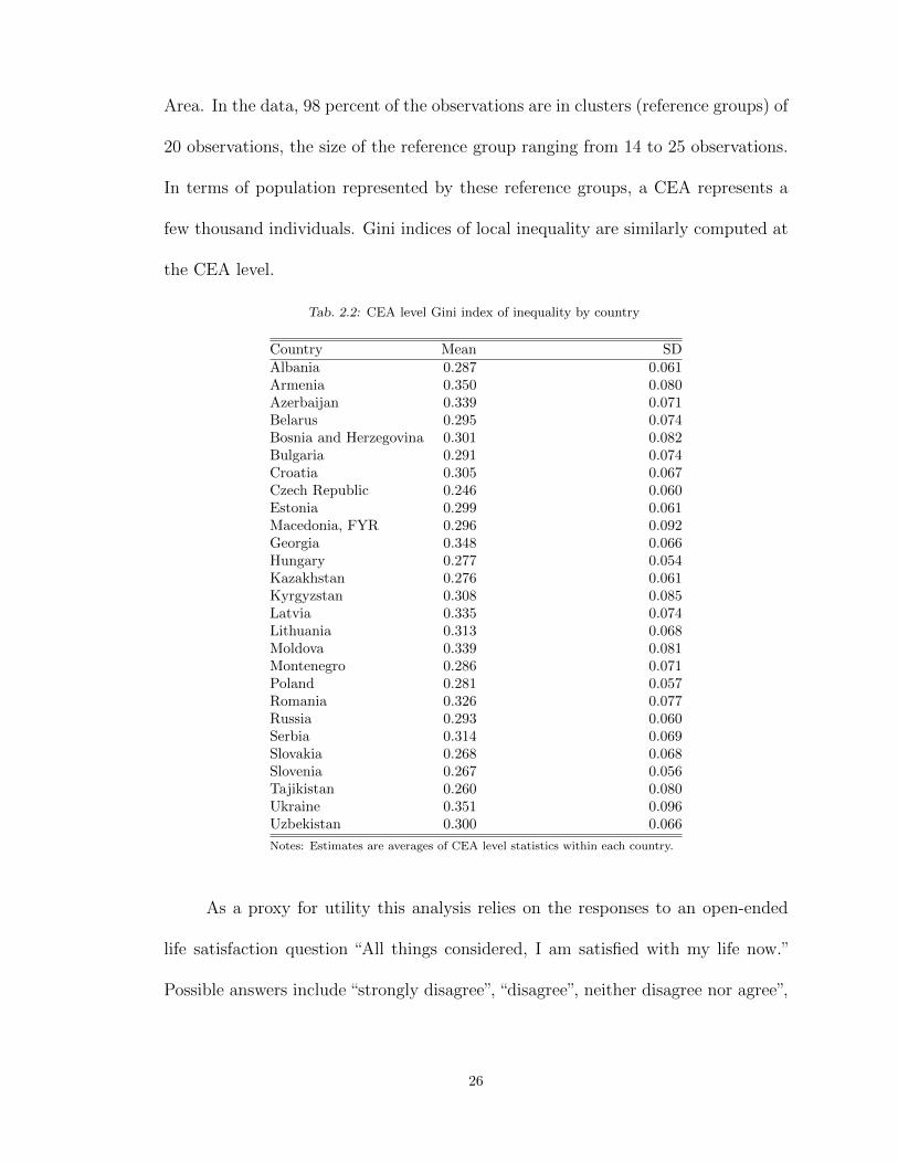
Area. In the data, 98 percent of the observations are in clusters (reference groups) of

20 observations, the size of the reference group ranging from 14 to 25 observations.

In terms of population represented by these reference groups, a CEA represents a

few thousand individuals. Gini indices of local inequality are similarly computed at

the CEA level.

Tab. 2.2: CEA level Gini index of inequality by country

Country Mean SDAlbania 0.287 0.061Armenia 0.350 0.080Azerbaijan 0.339 0.071Belarus 0.295 0.074Bosnia and Herzegovina 0.301 0.082Bulgaria 0.291 0.074Croatia 0.305 0.067Czech Republic 0.246 0.060Estonia 0.299 0.061Macedonia, FYR 0.296 0.092Georgia 0.348 0.066Hungary 0.277 0.054Kazakhstan 0.276 0.061Kyrgyzstan 0.308 0.085Latvia 0.335 0.074Lithuania 0.313 0.068Moldova 0.339 0.081Montenegro 0.286 0.071Poland 0.281 0.057Romania 0.326 0.077Russia 0.293 0.060Serbia 0.314 0.069Slovakia 0.268 0.068Slovenia 0.267 0.056Tajikistan 0.260 0.080Ukraine 0.351 0.096Uzbekistan 0.300 0.066

Notes: Estimates are averages of CEA level statistics within each country.

As a proxy for utility this analysis relies on the responses to an open-ended

life satisfaction question “All things considered, I am satisfied with my life now.”

Possible answers include “strongly disagree”, “disagree”, neither disagree nor agree”,

26

“agree”, “strongly agree.”9 In the overall sample 44 percent of respondents either

agreed or strongly agreed with the above statement.

In addition, this study employs a number of other attitudinal questions from

the survey, such as questions about the respondent’s opinion on factors that im-

portant for success in life, or on reasons why there is need in society today, or on

state’s involvement in reducing the gap between the rich and the poor. Finally,

the survey records a number of standard socio-demographic characteristics that are

normally found to be important determinants of subjective well-being. Summary

statistics the main variables are presented in Table 2.1. Estimates of the Gini indices

of inequality at CEA level for all countries in the sample are presented in Table 2.2.

2.4 Empirical analysis of inequality aversion and well-being

The discussion in section 2.2.2. is operationalised by means of the following

empirical specification:

h∗ijc = γyijc + λD(yijc) + βyrelijc +X ′ijcδ + εijc

where h∗ijc is latent satisfaction, yijc is the per capita consumption of household

i from Census Enumeration Area j in country c, D(yijc) is Yitzhaki’s measure of

relative deprivation, yrelijc = yijc − µjc, and µjc is the mean income of the reference

group. This is the empirical counterpart of U(yi) = yi + β(yi−µ) + (α+ β)D(yi) in

Section 2.2.2, estimated conditional on a set of individual, household, and geographic

covariates. The correspondence between the parameters α and β of the theoretical

model in section 2.2.2. and the coefficients of the empirical specification is as follows:

λ = α+ β, where β captures, as before, aversion to advantageous inequality, and α

9 Overall, 2 percent of the sample replied “don’t know” or “not applicable” and are excluded from the analysis.

27

captures aversion to disadvantageous inequality. The joint test of inequality aversion

is the test of the null hypothesis λ = 0, and λ < 0 (equivalent to α+β < 0) indicates

inequality averse preferences based on this joint test. Moreover, β < 0 indicates

aversion to advantageous inequality, and λ− β < 0 (equivalent to α < 0), indicates

aversion to disadvantageous inequality.

To account for a number of confounding factors, the FS model is estimated

conditional on a set X of variables (including a constant) that have been previously

found to explain variation in life satisfaction. These include a second degree poly-

nomial in age (to account for the well-known U-shaped relationship between age

and life satisfaction), sex and education of the respondent, whether the respondent

is the head of the household, household size, area of residence (rural vs urban), re-

spondent’s employment status and religious affiliation. A dummy for whether there

were two respondents in the household is also included to account for imperfect

knowledge of household expenditures by respondents who are not heads of house-

hold.10 To account for differences in subjective well-being across countries, a set of

country dummies is also included in the regressions, such that estimates are based

on within-country variation.11

Regressions also include dummies indicating the nature of respondent’s (self-

reported) mobility during the 1989-2006 period, whether downward, upward or sta-

10 Note that in cases when there is only one respondent, the head of household and most knowledgeable adultare different household members in in 15 percent of cases, which is why dummies for both household head and tworespondents are included.11 Pischke (2010) investigates whether the correlation between income and life satisfaction in a cross-sectional

setting can be viewed as causal, with causality running from income to satisfaction. Based on data from the USGeneral Social Survey (GSS), the European Social Survey (ESS) and the German Socio Economic Panel (GSOEP),and relying on industry wage differentials as instruments for family income, he runs a number of tests, includingcomparisons of results based on life satisfaction with those based on job satisfaction, looking at the life satisfactionof the wives, using husbands industry as the instrument, as well as using individual fixed effects. His results areconsistent with the conclusion that the cross-sectional relationship between income and life satisfaction is mostlycausal, rather than being the outcome of unobservables or reverse causality.

28

ble (baseline). These mobility dummies are based on the answers to a ladder question

that asks the respondent to place herself today (in 2006), and similarly in 1989, on

a “ten-step ladder where on the bottom, the first step, stand the poorest people and

on the highest step, the tenth, stand the richest.” The inclusion of these dummies

allows also for an inter-temporal reference point, which has been found to be im-

portant in the literature on adaptation (Frederick and Loewenstein, 1999; Frey and

Stutzer, 2001; Di Tella et al., 2003; Di Tella et al., 2010). Senik (2009), for instance,

finds comparisons with own economic situation prior to 1989 to still be an important

determinant of subjective well-being 15 years into the transition process in Eastern

Europe. Since movements from the 1st step to the 2nd, and from the 5th step to

the 6th, for instance, can be perceived as qualitatively different, and because those

at the bottom (top) in 2006 are more likely to have experienced downward (upward)

mobility in the past, the specification also controls for the respondent’s placement

on the current (2006) economic ladder.

It should be noted, however, that the test of loss-aversion based on this inter-

temporal reference point should be viewed as merely suggestive, since life satisfaction

and the placement on the economic ladder can be jointly determined and it is difficult

to rule out endogeneity completely in a cross-sectional setting with the data at hand.

The influence of unobservable traits that may influence both the response to the life

satisfaction question and to the economic ladder question is mitigated partly by the

fact that the test of loss aversion is based on the difference between the 2006 ladder

and the 1989 ladder and to the extent that the unobservable traits affect responses

to both ladder questions in a similar way, the bias will be at least partly mitigated.

29

An alternative test is also provided in Section 2.4.3, where the dependent variable

is preference for redistribution instead of satisfaction with life.

Given the ordinal nature of observed life satisfaction, it is assumed that hi = k

if τk−1 ≤ h∗i < τk, where τk are unknown cut points with τ0 = −∞ and τ5 = ∞.

It is further assumed that Pr[hi = k] = Pr[τk−1 ≤ h∗i < τk] = F (τk − X̃′iζ) −

F (τk−1−X̃′iζ), where εijk is assumed logistic distributed with cumulative distribution

F (z) = ez/(1 + ez).12 Finally, errors are allowed to be correlated within primary

sampling units.

The above model is the baseline FS specification for the empirical test of

inequality aversion. Estimates from this model (Table 2.3), reveal that both for

the full sample and for regional subsamples other than South-Eastern Europe 13

respondents are averse to inequality (λ < 0), controlling for a number of character-

istics commonly found to be important determinants of life satisfaction.14 Moreover,

estimates suggest aversion to both disadvantageous inequality and to advantageous

inequality, as suggested by the Fehr and Schmidt (1999) model.15 In practical terms,

the estimates of the baseline model imply that a rank-preserving progressive transfer

resulting in a 1 unit (USD 1,000/year/per person) increase in relative deprivation,

holding own income and mean group income constant, would be associated with a

12 Here X̃ designates the full vector of covariates.13 The group of EU members comprises Czech Republic, Estonia, Hungary, Latvia, Lithuania, Poland, Slovakia

and Slovenia; the group of non-EU South-Eastern European countries includes Albania, Bosnia and Herzegovina,Bulgaria, Croatia, FYR Macedonia, Montenegro, Romania and Serbia; the group of CIS countries is comprised of11 countries, including all former Soviet Republics with the exception of the Baltic States (included in EU) andTurkmenistan, for which data were not available.14 In the case of South-Eastern Europe the results are similar, albeit less precisely estimated. Moreover, if Bulgaria

and Romania, who were about to join the European Union when the LiTS survey was fielded, are grouped insteadwith the other EU member states, then λ < 0 in the South-East European sub-sample as well.15 There is a large literature that looks at relative status effects by estimating equations like hi = ρyi + ψ(yi −µ) +X′iζ + υi. It is commonly found that ψ > 0 (for a review, see Clark et al., 2008), although Senik (2004) findsthat ψ < 0 based on data from Russia. The parameter ψ in such models should not be compared to the structuralparameter β in the FS specification as they identify different things. Indeed, if Yitzhaki’s RD is removed from thebaseline model reported in table 2.3, the coefficient on the relative income variable becomes positive, albeit notstatistically significant.

30

Tab. 2.3: Baseline FS model of inequality aversion, by region

(1) (2) (3) (4)Own expenditures (γ) 0.017*** 0.016** 0.016* 0.023*

(0.004) (0.005) (0.008) (0.010)Relative expenditures (β) -0.016** -0.018** -0.008 -0.025*

(0.005) (0.006) (0.010) (0.012)Yitzhaki’s RD (λ) -0.030*** -0.030*** -0.022 -0.046**

(0.006) (0.007) (0.012) (0.015)Age 0.000 0.001*** 0.000 -0.001**

(0.000) (0.000) (0.000) (0.000)Male 0.008* 0.002 0.008 0.012*

(0.003) (0.006) (0.006) (0.006)Education level: secondary ref. ref. ref. ref.Compulsory -0.015** -0.014 -0.029** 0.003

(0.005) (0.009) (0.010) (0.008)Vocational -0.004 0.002 -0.017 -0.002

(0.005) (0.008) (0.010) (0.007)University 0.026*** 0.039*** 0.015 0.020**

(0.005) (0.008) (0.010) (0.007)HH size 0.006*** 0.010*** 0.010*** 0.004*

(0.001) (0.003) (0.003) (0.002)Employed 0.019*** 0.014 0.018* 0.021**

(0.004) (0.007) (0.008) (0.007)Head of HH -0.008 -0.013 -0.002 -0.006

(0.005) (0.008) (0.010) (0.009)Two respondents 0.008 0.005 0.014 0.010

(0.005) (0.008) (0.010) (0.009)Current welfare ladder 0.043*** 0.039*** 0.046*** 0.042***

(0.002) (0.003) (0.003) (0.003)Mobility during 1986-2006: stable ref. ref. ref. ref.Downward mobility 1989-2006 -0.071*** -0.077*** -0.074*** -0.062***

(0.006) (0.009) (0.010) (0.010)Upward mobility 1989-2006 0.019** 0.018* 0.009 0.026*

(0.006) (0.007) (0.015) (0.011)Religion: atheist/agnostic ref. ref. ref. ref.Christian 0.002 -0.017* 0.006 0.038**

(0.007) (0.008) (0.017) (0.015)Muslim 0.004 -0.054 0.002 0.051**

(0.012) (0.044) (0.020) (0.019)Other -0.031* -0.045** 0.045 -0.038

(0.014) (0.016) (0.038) (0.033)Urban -0.003 -0.014 -0.003 0.007

(0.006) (0.008) (0.012) (0.010)Pseudo R-squared 0.109 0.098 0.091 0.116Obs 23783 7117 7306 9360α -0.014 -0.012 -0.014 -0.021Prob>chi2 0.000 0.013 0.106 0.014

Notes: Average marginal effects. Robust standard errors, clustered at reference group level in parentheses.Dependent variable: life satisfaction. Column (1) - full sample; (2) - EU; (3) - SEB; (4) - CIS. Countrydummies included but not reported. Baseline categories: education - secondary; mobility - none; religion- atheist/agnostic The structural parameter α is calculated based on regression estimates. Significance: *p<0.05, ** p<0.01, *** p<0.001.

31

3 percentage points lower probability of reporting above average life satisfaction. A

one standard deviation increase in relative deprivation (USD 620) would be associ-

ated with a 1.9 percentage points lower probability of reporting above neutral life

satisfaction. For the CIS subsample a one standard deviation increase in relative

deprivation would be associated with a 2.9 percentage points lower probability of

reporting above neutral life satisfaction.

The other variables in the model have expected signs. Age and life satisfaction

exhibit a U-shaped relationship with a minimum at around the age of 48, which is

consistent with other studies in the happiness economics literature (Graham 2010).16

Men report higher satisfaction levels in the overall sample and in the CIS sub-sample,

which is again consistent with other findings from Transition Economies, although

in Western Europe the opposite tends to be the case (Graham 2010). Satisfaction

with life increases with the education level of the respondent, and is also higher for

those who are employed and for those from larger households.

The estimates also suggest an important inter-temporal reference point - down-

ward mobility during the 1989-2006 period is associated with lower satisfaction with

life, holding current position on the income ladder constant. The coefficient on the

upward mobility variable is positive, but smaller in magnitude, and the difference

is statistically significant in all four cases. Even though 15 years elapsed between

the collapse of the Soviet Union and the LiTS survey, the pre-transition standard of

living still looms large in people’s memories (see also Senik 2009). These results are

consistent with loss aversion (Kahneman and Tversky, 1979) and with adaptation

16 Note that while both age and age squared are included in the regression, the average marginal effect for age isreported, which account for the fact that age enters as a second degree polynomial. The small average marginaleffect is consistent with the U-shaped relationship between age and life satisfaction.

32

being more complete in the domain of gains from the reference point relative to the

domain of losses (Arkes et al, 2006).

A modified version of the above model is estimated next, where D(yijc) is sub-

stituted with Gjc, the Gini coefficient of inequality defined at the reference group

level. This specification aims to test whether inequality aversion can also be cap-

tured by looking at the relationship between an aggregate index of inequality and

individual life satisfaction, conditional on the same set of control variables. There

are two main reasons for choosing the Gini index in favour of some other aggregate

index of inequality as, for instance, Theil. First, the Gini index is most commonly

used index to measure inequality, and it is also the index that is generally employed

in the studies that estimate a relationship between the individual satisfaction and

the level of inequality. More importantly, Gini is the theoretically relevant index of

inequality, implied by the FS model. To see this, note that given no within group

variation in the Gini index, a regression of individual satisfaction on the Gini in-

dex essentially looks at the relationship between mean group satisfaction and the

group’s index of inequality. Aggregating the FS utility specification to group level

gives group satisfaction as a function of mean group income and the group’s Gini

index of inequality (see section 2.4.2).

The results are reported in Table 2.4.17 The Gini coefficient has no association

with life satisfaction at conventional significance levels, which is in line with the

earlier results by Senik (2004) and Graham and Felton (2006) who similarly find no

relationship between inequality and well-being. As the discussion in section 2.2.2.

17 In this and all of the tables that follow the conditioning vector remains the same as in Table 3, but the estimatesare omitted to conserve space.

33

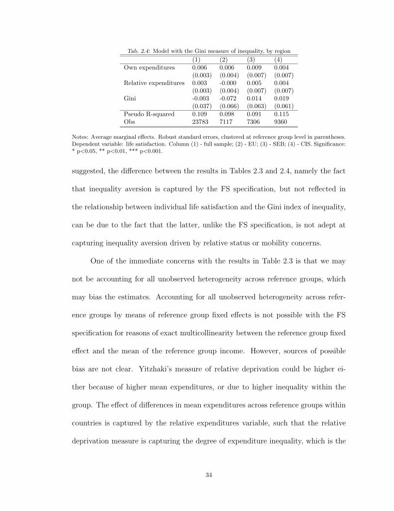
Tab. 2.4: Model with the Gini measure of inequality, by region

(1) (2) (3) (4)Own expenditures 0.006 0.006 0.009 0.004

(0.003) (0.004) (0.007) (0.007)Relative expenditures 0.003 -0.000 0.005 0.004

(0.003) (0.004) (0.007) (0.007)Gini -0.003 -0.072 0.014 0.019

(0.037) (0.066) (0.063) (0.061)Pseudo R-squared 0.109 0.098 0.091 0.115Obs 23783 7117 7306 9360

Notes: Average marginal effects. Robust standard errors, clustered at reference group level in parentheses.Dependent variable: life satisfaction. Column (1) - full sample; (2) - EU; (3) - SEB; (4) - CIS. Significance:* p<0.05, ** p<0.01, *** p<0.001.

suggested, the difference between the results in Tables 2.3 and 2.4, namely the fact

that inequality aversion is captured by the FS specification, but not reflected in

the relationship between individual life satisfaction and the Gini index of inequality,

can be due to the fact that the latter, unlike the FS specification, is not adept at

capturing inequality aversion driven by relative status or mobility concerns.

One of the immediate concerns with the results in Table 2.3 is that we may

not be accounting for all unobserved heterogeneity across reference groups, which

may bias the estimates. Accounting for all unobserved heterogeneity across refer-

ence groups by means of reference group fixed effects is not possible with the FS

specification for reasons of exact multicollinearity between the reference group fixed

effect and the mean of the reference group income. However, sources of possible

bias are not clear. Yitzhaki’s measure of relative deprivation could be higher ei-

ther because of higher mean expenditures, or due to higher inequality within the

group. The effect of differences in mean expenditures across reference groups within

countries is captured by the relative expenditures variable, such that the relative

deprivation measure is capturing the degree of expenditure inequality, which is the

34

Tab. 2.5: Specification with reference group fixed effects

(1) (2) (3) (4)Expenditures (γ + β) 0.001 -0.013 0.020* -0.002

(0.005) (0.007) (0.008) (0.007)RD (λ) -0.057*** -0.069*** -0.049 -0.058*

(0.013) (0.018) (0.025) (0.028)Pseudo R-squared 0.122 0.126 0.127 0.121Obs 22815 7023 6962 8830

Notes: Conditional fixed effects logistic regressions. Average marginal effects. Robust standard errors,clustered at reference group level in parentheses. Dependent variable equals 1 if respondent agrees orstrongly agrees with All things considered, I am satisfied with my life now, and zero if the respondentstrongly disagrees, disagrees or neither disagrees nor agrees. Column (1) - full sample; (2) - EU; (3) - SEB;(4) - CIS. Significance: * p<0.05, ** p<0.01, *** p<0.001.

primary interest of this analysis. The estimates could be biased however if, for

instance, a particular characteristic were more (less) common within groups with

higher inequality, and also negatively (positively) associated with subjective well-

being in ways that are not captured by mean expenditure differences across groups

or other control variables.

To account for all unobserved heterogeneity across reference groups a condi-

tional fixed effects logit model is estimated (Table 2.5) in which matching is done

within reference groups.18 This is similar to the analysis of Eibner and Evans (2005),

although they rely on a linear specification. In this specification λ is identified out of

within reference group variation, accounting for all heterogeneity in unobserved ref-

erence group characteristics. The test for inequality aversion is the joint test of the

null hypothesis λ = 0. The estimates in Table 2.5 confirm the presence of inequality

aversion in individual preferences, both in the overall sample and in the EU and

CIS regional sub-samples. In this specification a one standard deviation increase in

relative deprivation is associated with a 3.6 percentage points lower probability of

18 Since this model is binary, the dependent variable is transformed into a dummy (hb) that evaluates to 1 if therespondent either agrees or strongly agrees with the life satisfaction statement, and zero otherwise. The matchinghere is mj : nj , i.e. generally in group j (strictly, at least in 1 group) there are mj > 1 observations where hb = 1and nj observations for which hb = 0. Note also that the coefficient on the own expenditures variable in Table 2.5is the counterpart of the (γ + β) in Table 2.4 and not of γ alone.

35

Tab. 2.6: Further robustness checks

(1) (2)Minimum income (γ) -0.001

(0.003)Relative min income (β) 0.002

(0.003)RD (minimum income) (λ) -0.001

(0.004)Own expenditures (γ) 0.968***

(0.126)Relative expenditures (β) -0.300*

(0.152)Yitzhaki’s RD (λ) -0.136

(0.148)R-squared 0.556Pseudo R-squared 0.108Obs 23730 24199α -0.003 0.164Prob>F 0.214 0.005

Notes: Average marginal effects in (1) OLS estimates in (2). Robust standard errors, clustered at referencegroup level in parentheses. Dependent variable in column (1): life satisfaction. Dependent variable in (2)is the reported minimum amount of money per capita needed to make ends meet. Significance: * p<0.05,** p<0.01, *** p<0.001.

reporting above neutral life satisfaction in the overall sample, and an 5.3 percentage

points lower probability in the EU subsample.

As a further robustness check, in column (1) of Table 2.6 the same regression as

above is run with relative deprivation defined in terms of minimum income instead

of actual household expenditures. Minimum income is reported in response to the

question ‘Living in the dwelling and doing what you do, what would be the minimum

amount of money that this household would need to make ends meet at the end

of each month.’19 The estimates suggest that inequality in perceived necessary

minimum income does not have an effect on utility. Upon reflection, this is not

surprising. The income that is perceived as being the necessary minimum is likely

to already reflect the relative status concerns that may be present. Indeed, as

the estimates in column (2) suggest, α < 0 and β > 0 such that disadvantageous

19 Minimum income is converted to per capita units.

36

(advantageous) inequality in expenditures has a positive (negative) effect on the

amount of money deemed to be the necessary minimum.

2.4.1 What is driving inequality aversion?

What could be the source of inequality aversion? One possibility is that in-

dividuals are intrinsically averse to inequality in outcomes, such that inequality is

utility-decreasing even when it can be considered as just from the social justice

perspective. Another possibility is that inequality aversion is the outcome of per-

ceptions of unfairness with regard to the processes that determine the distribution

of fortunes. With regard to the results of laboratory experiments, the World De-

velopment Report 2006 notes that “it is possible to speculate that the aversion to

very unequal payoff distributions in the Ultimatum Game arises from the arbitrary

and unequal nature of the endowments (or power) implicit in the initial allocation

of the roles of Proposer and Responder” (World Bank 2005: 81). Graham and Fel-

ton (2006) argue that inequality exhibits a negative impact on happiness in Latin

America because it signals persistent unfairness. Alesina, DiTella and MacCulloch

(2004) similarly argue that the strong inequality aversion in Europe is due to a

lower degree of mobility in the society, whereas Americans believe that poverty can

be escaped through hard work. Runciman (1972:22) notes that relative deprivation

is brought about by the upsetting of expectations, such as for instance, when stable

expectations are disappointed. The transition period certainly can be described as

the time when stable expectations of many individuals had been disappointed.

An empirical test of this hypothesis is possible with the LiTS data. Respon-

dents were asked the following question: “In your opinion, what is the main reason

37

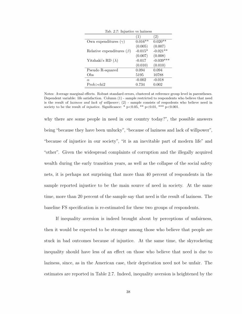
Tab. 2.7: Injustice vs laziness

(1) (2)Own expenditures (γ) 0.016** 0.020**

(0.005) (0.007)Relative expenditures (β) -0.015* -0.021**

(0.007) (0.008)Yitzhaki’s RD (λ) -0.017 -0.039***

(0.010) (0.010)Pseudo R-squared 0.094 0.094Obs 5195 10788α -0.002 -0.018Prob>chi2 0.734 0.002

Notes: Average marginal effects. Robust standard errors, clustered at reference group level in parentheses.Dependent variable: life satisfaction. Column (1) - sample restricted to respondents who believe that needis the result of laziness and lack of willpower ; (2) - sample consists of respodents who believe need insociety to be the result of injustice. Significance: * p<0.05, ** p<0.01, *** p<0.001.

why there are some people in need in our country today?”, the possible answers

being “because they have been unlucky”, “because of laziness and lack of willpower”,

“because of injustice in our society”, “it is an inevitable part of modern life” and

“other”. Given the widespread complaints of corruption and the illegally acquired

wealth during the early transition years, as well as the collapse of the social safety

nets, it is perhaps not surprising that more than 40 percent of respondents in the

sample reported injustice to be the main source of need in society. At the same

time, more than 20 percent of the sample say that need is the result of laziness. The

baseline FS specification is re-estimated for these two groups of respondents.

If inequality aversion is indeed brought about by perceptions of unfairness,

then it would be expected to be stronger among those who believe that people are

stuck in bad outcomes because of injustice. At the same time, the skyrocketing

inequality should have less of an effect on those who believe that need is due to

laziness, since, as in the American case, their deprivation need not be unfair. The

estimates are reported in Table 2.7. Indeed, inequality aversion is heightened by the

38

Tab. 2.8: Hard work vs political and criminal connections

(1) (2) (3) (4)Own expenditures (γ) 0.019** 0.018** 0.021*** 0.005

(0.007) (0.007) (0.006) (0.006)Relative expenditures (β) -0.014 -0.020* -0.023** 0.003

(0.009) (0.008) (0.007) (0.008)Yitzhaki’s RD (λ) -0.025* -0.043*** -0.036*** -0.005

(0.011) (0.010) (0.009) (0.011)Pseudo R-squared 0.111 0.103 0.109 0.111Obs 9070 7288 12845 4839α -0.011 -0.023 -0.014 -0.008Prob>chi2 0.091 0.001 0.016 0.175

Notes: Average marginal effects. Robust standard errors, clustered at reference group level in parentheses.Dependent variable: life satisfaction. Column (1) - Sample restricted to respondents who believe thateffort and hard work are the most important factor to succeed in life now ; (2) - respondents who believepolitical or criminal ties to be the most important factor to succeed in life now ; (3) - respondents who statethat effort and hard work were the most important factor to succeed in 1989 ; (4) - respodents who believepolitical, criminal ties to have been the main determinant of success in 1989. Significance: * p<0.05, **p<0.01, *** p<0.001.

perception of unfairness. Respondents who believe that need is caused by laziness

do not exhibit inequality averse preferences, unlike respondents who believe that

need is caused by injustice.

Respondents were additionally asked about the factors that are important to

succeed in life today, and also about factors important for success prior to 1989.

Here the focus is on those who reported the main factor for success to be ‘effort and

hard work’ on the one hand, and ‘political connections / criminal and corrupt ties’

on the other hand. Estimates reported in Table 2.8 suggest aversion to inequality

among those who believe success today to be determined by political connections or

criminal ties to be more prominent than among those who believe that hard work

is the main determinant of success.

When similar regressions are run for attitudes toward success prior to 1989,

the results are reversed. Inequality averse preferences are observed among those

who believe that prior to 1989 hard work was the main factor of success, but not

39

among respondents who believed that before the transition period started political

connections were important. In other words, it seems that those who believed in the

importance of hard work in the past associate the inequality in the distribution today

as not being the result of hard work, but rather of corruption, which is why it has a

negative effect on utility. Those who think that political / criminal connections were

important even before 1989 were perhaps less disturbed by the rampant corruption

during the transition years. Why should there be a difference between the results in

columns (2) and (4) if inequality is corruption-driven? Recall Runciman’s argument

that relative deprivation is heightened when expectations are being disappointed. It

is likely that for the subgroup in column (4) the expectations were not disappointed,

if they already saw connections as the main key to success even before 1989.

It should be noted that it is possible for perceptions of the main drivers of

success or need in society to be systematically linked, through some unobservables,

with life satisfaction. With the existing data it is difficult to eliminate this possi-

bility, such that the estimates in Tables 2.7 and 2.8 should be viewed as suggestive.

In section 2.4.3 I re-estimate the model with the preference for inequality as the

dependent variable instead of life satisfaction. The results are consistent with those

in tables 2.7 and 2.8. While this alone does not resolve the possible endogeneity, it

is somewhat reassuring that the estimates are robust to alternative specifications of

the dependent variable.

In addition to institutional factors, it may also be the case that aversion to

inequality is driven by the personal fortunes throughout the turbulent transition

years. As suggested by estimates in Table 2.3, lower status on the socio-economic

40

Tab. 2.9: Winners and losers of the transition process

(1) (2)Own expenditures (γ) 0.025*** 0.005

(0.006) (0.005)Relative expenditures (β) -0.025*** -0.004

(0.007) (0.006)Yitzhaki’s RD (λ) -0.039*** -0.017*

(0.009) (0.007)Pseudo R-squared 0.088 0.063Obs 14147 4786α -0.014 -0.014Prob>chi2 0.014 0.002

Notes: Average marginal effects. Robust standard errors, clustered at reference group level in parentheses.Dependent variable: life satisfaction. Column (1) - downwardly mobile sample; (2) - upwardly mobilesample. Significance: * p<0.05, ** p<0.01, *** p<0.001.

ladder today relative to 1989 is negatively associated with reported life satisfaction.

One could hypothesize, as do Graham and Felton (2006), that attitudes toward

inequality will be coloured by one’s own mobility trajectory during the transition

period. Aversion to inequality may be higher, in particular, among those who moved

down the socio-economic ladder during the 1989-2006 period, according to their

own perceptions, and, correspondingly, lower among the upwardly mobile group.

Estimates in Table 2.9 do not necessarily bear out this hypothesis, however. The FS

specification is re-estimated separately among those who reported being on a lower

ladder step in 2006 than in 1989 (column 1), and those who either stayed in place or

moved up the socio-economic ladder (column 2). In particular in both cases α < 0,

and λ < 0.

Future mobility prospects can also influence one’s preferences for the degree

of inequality in society. Benabou and Ok (2001) propose a model in which it can be

rational for poor individuals today to oppose redistribution because they expect to

move up the economic ladder in the future (known as the prospect of upward mobility

hypothesis). This hypothesis is explored in detail in Chapter 3 of this dissertation,

41

Tab. 2.10: Inequality aversion among young and old respodents

(1) (2) (3)Own expenditures (γ) 0.010 0.013* 0.024***

(0.006) (0.006) (0.006)Relative expenditures (β) -0.006 -0.014 -0.023**

(0.007) (0.007) (0.008)Yitzhaki’s RD (λ) -0.016 -0.030** -0.038***

(0.008) (0.010) (0.010)Pseudo R-squared 0.096 0.110 0.099Obs 9022 8324 8656α -0.010 -0.016 -0.014Prob>chi2 0.077 0.010 0.016

Notes: Average marginal effects. Robust standard errors, clustered at reference group level in parentheses.Dependent variable: life satisfaction. Column (1) - bottom age tertile (respondents aged 37 or younger);(2) - middle age tertile (38-56); (3) top tertile (57+ age group). Significance: * p<0.05, ** p<0.01, ***p<0.001.

as respondents’ mobility aspirations are are not available in the data LiTS 2006 data

used in this analysis.

It is still possible to hypothesise that younger cohorts may be more optimistic

about future economic mobility, and hence less averse to inequality, because it may

be easier for them to develop or adapt their skill set to match the changing require-

ments of the labour market. To test this empirically I split the sample into three

groups based on age tertiles, which corresponds to the following groups: respondents

aged 37 or under, respondents in the 38-55 age group, and respondents aged 56 or

higher) and re-estimate the FS model for each of these age groups. This split is

arbitrary, but it ensures that the first group was 21 or younger in 1989, such that

they completed their tertiary education and entered the labour market after the

start of transition. The results are consistent with the above reasoning - inequality

averse preferences are largely absent in the under 35 age group, whereas in the other

two groups the joint test of no inequality aversion rejects the null of λ = 0. These

results are also consistent with the findings of Bellemare et al. (2008).

42

2.4.2 Implications for social welfare

Consider an additive social welfare function of the formW (y) =´ y∗

0u(z)dF (z).

Aggregating to the level of reference groups, we obtain:

Wj(y) = µj(1− θGj)

where µj denotes mean expenditures in cluster j, Gj is the group’s Gini index of

inequality, and θ = −(α+ β). Note that in the case of inequality averse preferences

θ > 0, as confirmed by the estimates in section 2.4.1, such that higher within-

group inequality lowers social welfare. Note also that W (y) resembles Atkinson’s

formulation W = µ(1 − I), where µ is mean group income and I is the group’s

measure of inequality. However, it is important to note that Atkinson’s social welfare

function is normative in character and has inequality aversion built into it, such that

it allows for reductions in mean income for purposes of greater equality. The social

welfare function adopted here, on the other hand, is utilitarian in nature, and is

not per se concerned with inequality. The fact that the social welfare function

allows for tradeoffs between the size of the pie and the degree of inequality in its

distribution stems from inequality aversion in individual preferences. It is clear from

this formulation that a redistribution of income via a rank-preserving Pigou-Dalton

transfer that decreases inequality will lead to an increase in social welfare, whereas

a regressive transfer that increases inequality would reduce social welfare.

This result is confirmed in Table 2.11, which presents estimates of CEA-level

OLS regressions of mean CEA life satisfaction on mean CEA expenditures, CEA

Gini index of inequality, as well as mean values of control variables collapsed to the

43

Tab. 2.11: Inequality and well-being across groups

(1) (2) (3) (4)Mean group expenditures 0.108*** 0.113*** 0.072*** 0.033

(0.013) (0.017) (0.019) (0.017)Group Gini -1.362*** -0.594** -0.409* -0.252

(0.206) (0.182) (0.186) (0.160)Country dummies no yes yes yesSocio-demographic controls no no yes yesMobility controls no no no yesR-squared 0.078 0.457 0.476 0.567Obs 1350 1350 1350 1349

Notes: OLS estimates. Robust standard errors in parentheses. Dependent variable is mean reference grouplife satisfaction. Significance: * p<0.05, ** p<0.01, *** p<0.001.

level of CEAs. Group level life satisfaction is positively associated with the average

group expenditures and negatively associated with the group Gini (column 1). The

negative association between average life satisfaction and inequality is maintained if

country dummies are added to the specification, such that the estimates draw only

on within-country variation (column 2), and when mean values of other covariates

other than the mobility and current economic rank are accounted for (column 3).

The relationship between inequality and life satisfaction becomes insignificant when

we control for the 1989-2006 mobility experience (column 4). This latter result is not

surprising once it is noted that movements up and down the socio-economic ladder

since 1989 (and in particular wage losses as the result of the post-1989 economic

contraction) are likely among the key determinants of the level of inequality today.

2.4.3 Inequality aversion and support for redistribution

Since inequality aversion is inherent in individual preferences, and since these

preferences imply that redistributive policies have a positive effect on social welfare,

it should be the case that inequality averse individuals should favour redistributive

policies. Indeed, Alesina et al. (2004) argue that Europeans, whom they find to be

44

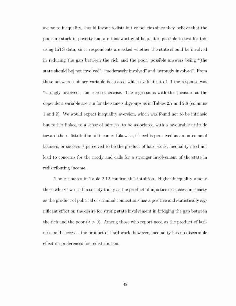
averse to inequality, should favour redistributive policies since they believe that the

poor are stuck in poverty and are thus worthy of help. It is possible to test for this

using LiTS data, since respondents are asked whether the state should be involved

in reducing the gap between the rich and the poor, possible answers being “[the

state should be] not involved”, “moderately involved” and “strongly involved”. From

these answers a binary variable is created which evaluates to 1 if the response was

“strongly involved”, and zero otherwise. The regressions with this measure as the

dependent variable are run for the same subgroups as in Tables 2.7 and 2.8 (columns

1 and 2). We would expect inequality aversion, which was found not to be intrinsic

but rather linked to a sense of fairness, to be associated with a favourable attitude

toward the redistribution of income. Likewise, if need is perceived as an outcome of

laziness, or success is perceived to be the product of hard work, inequality need not

lead to concerns for the needy and calls for a stronger involvement of the state in

redistributing income.

The estimates in Table 2.12 confirm this intuition. Higher inequality among

those who view need in society today as the product of injustice or success in society

as the product of political or criminal connections has a positive and statistically sig-

nificant effect on the desire for strong state involvement in bridging the gap between

the rich and the poor (λ > 0). Among those who report need as the product of lazi-

ness, and success - the product of hard work, however, inequality has no discernible

effect on preferences for redistribution.

45

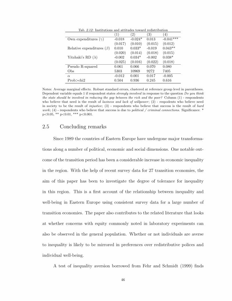
Tab. 2.12: Institutions and attitudes toward redistribution

(1) (2) (3) (4)Own expenditures (γ) -0.018 -0.024* 0.013 -0.041***

(0.017) (0.010) (0.015) (0.012)Relative expenditures (β) 0.010 0.033* -0.019 0.043**

(0.020) (0.014) (0.018) (0.015)Yitzhaki’s RD (λ) -0.002 0.034* -0.002 0.038*

(0.025) (0.016) (0.022) (0.018)Pseudo R-squared 0.061 0.066 0.070 0.080Obs 5303 10969 9272 7405α -0.012 0.001 0.017 -0.005Prob>chi2 0.504 0.936 0.245 0.616

Notes: Average marginal effects. Robust standard errors, clustered at reference group level in parentheses.Dependent variable equals 1 if respondent states strongly involved in response to the question Do you thinkthe state should be involved in reducing the gap between the rich and the poor? Column (1) - respondentswho believe that need is the result of laziness and lack of willpower ; (2) - respodents who believe needin society to be the result of injustice; (3) - respondents who believe that success is the result of hardwork ; (4) - respondents who believe that success is due to political / criminal connections. Significance: *p<0.05, ** p<0.01, *** p<0.001.

2.5 Concluding remarks

Since 1989 the countries of Eastern Europe have undergone major transforma-

tions along a number of political, economic and social dimensions. One notable out-

come of the transition period has been a considerable increase in economic inequality

in the region. With the help of recent survey data for 27 transition economies, the

aim of this paper has been to investigate the degree of tolerance for inequality

in this region. This is a first account of the relationship between inequality and

well-being in Eastern Europe using consistent survey data for a large number of

transition economies. The paper also contributes to the related literature that looks

at whether concerns with equity commonly noted in laboratory experiments can

also be observed in the general population. Whether or not individuals are averse

to inequality is likely to be mirrored in preferences over redistributive polices and

individual well-being.

A test of inequality aversion borrowed from Fehr and Schmidt (1999) finds

46

considerable support for aversion to inequality in individual preferences, and this

result holds across a number of specifications, and also across regional subsets of

countries. The benefit of this model is that it can detect aversion to inequality that

is driven by status and mobility considerations, a setting where aggregate inequality

measures provide little help. Indeed, this study found that the Gini index was

unable to capture this negative effect of inequality on well-being. The results in this

chapter thus caution against the common practice of looking at the effect of economic

inequality on well-being by means of the empirical relationship between individual

well-being and aggregate inequality indices calculated over some geographic space.

Building on the work by Roemer (2000) and earlier philosophical studies (Sen

1980; Dworkin 1981; Arneson 1989; Cohen 1989), a number of recent papers distin-

guish between overall inequality and inequality of opportunity. (Bourguignon et al.

2003; Roemer et al. 2003; Ooghe et al. 2007; Checchi and Peragine 2009; Cogneau

and Mesple-Somps 2008; Ferreira and Gignoux 2008; Ferreira et al. 2008, 2010;

Lefranc et al. 2008, 2009). These studies stress that it is inequality of opportunity

that is morally objectionable, as opposed to inequalities generated by differences in

effort. While I do not formalise a concept of inequality of opportunity in this study,

the evidence this paper presents is suggestive of inequality of opportunity driving

attitudes toward overall economic inequality in transition economies. Aversion to

inequality is found not to be intrinsic, but rather tied to a concern with fairness

in the institutions underlying the distribution of fortunes in society. The relation-

ship between redistributive preferences (and expectations of social mobility), and a

Rawlsian concept of inequality of opportunity is also examined in Chapter 3 of this

47

dissertation.

Inequality averse preferences imply a negative relationship between inequality

and social welfare, even when the underlying social welfare function is utilitarian in

character and is not intrinsically concerned with inequality. This suggests that in-

equality aversion should be associated with demands for redistributive policies. Con-

sistent with this intuition, the LiTS data confirm the association between inequality

and demands for strong government involvement in bridging the gap between the

rich and the poor, but only when inequality is perceived to be unfair.

48

3 Prospects of upward mobility, inequality of opportunity andpreferences for redistribution

3.1 Introduction

The extent to which the brunt of the austerity measures implemented in re-

sponse to the recent financial crisis should fall on the wealthy is at the forefront

of policy debates on both sides of the Atlantic. The arguments in favour of taxing

the rich stem partly from the fact that they have benefited disproportionately from

globalisation. Indeed, income inequality increased considerably in many European

countries and in the United States over the past two decades, especially on account

of rapidly rising incomes at the top of the income distribution (Piketty and Saez

2003; OECD 2008). The increase in income inequality has been especially rapid in

Transition Economies since the early 1990s. It is thus not surprising that in these

countries more than 70 percent of adults believed that the gap between the rich

and the poor should be reduced, according the 2010 round of the Life in Transition

Survey (LiTS II). Even among those who placed themselves in the top three rungs

of a ten-step economic ladder more than 60 percent shared this view.

Yet, the link between high inequality and calls for redistribution is not auto-

matic. European governments have traditionally been more redistributive than that

of the United States despite lower levels of income inequality in Europe. Alesina,

DiTella and MacCulloch (2004) found that higher income inequality has a negative

effect on life satisfaction in Europe but not in the United States, and suggested that

the difference is due to perceptions of higher social mobility in the United States.

Notably, such perceptions of social mobility are not matched by reality - social mo-

49

bility in the United States is in fact lower than in European countries (OECD 2010)

- but it is precisely perceived social mobility that matters for life satisfaction and

preferences for redistribution at any given point in time.

Benabou and Ok (2001) propose a theoretical model in which the prospect

of upward mobility (POUM) for individuals who are poorer than average, and in

particular the expectation of being richer than average in the future, can under

certain conditions lead them to oppose lasting redistribution. These conditions

include requirements that voters have a reasonably low level of risk aversion, be

reasonably farsighted, and that fiscal policy set today can be expected to persist

into future periods.

This paper aims to empirically assess the POUM hypothesis based on compara-

ble data for all Transition Economies and a number of Western European countries.

It contributes to, and aims to improve upon, the existing empirical literature on

social mobility and preferences for redistribution. To my knowledge this is the first

study to investigate the relationship between social mobility and redistributive pref-

erences for a large set of Eastern European countries. Ravallion and Lokshin (2000)

provide some evidence based on Russian data from the mid-1990s.

The results from the overall sample of countries suggest that the prospects of

upward mobility are indeed associated with a lower preference for redistribution, but

only if the degree of risk aversion is low. The POUM hypothesis is then confirmed

for the sub-sample of countries that are EU members, whereas it does not hold in

the non-EU Transition Economies. The paper then looks in more detail at the deter-

minants of perceived future social mobility. The main question is whether mobility

50

aspirations are affected by inequality of opportunity in key dimensions of life such as

getting a university education or getting a job. The results suggest that inequality

of opportunity does indeed dampen aspirations of future upward mobility, but only

for the disadvantaged segments of the population - those who cannot overcome the

obstacles of an uneven playing field through personal connections.

The rest of the paper is structured as follows: section 3.2 briefly describes the

existing empirical studies that test the POUM hypothesis. Section 3.3 describes the

proposed empirical model. Section 3.4 discusses the data used in the analysis. Main

results are presented in section 3.5. Section 3.6 examines the link between social

mobility and inequality of opportunity. Section 3.7 concludes.

3.2 Empirical strategy

3.2.1 Data requirements and existing studies

The aim of this paper is to test empirically whether individuals who are poorer

than average in the present, but who expect to be richer than average in the future

exhibit a reduced level of support for redistributive policies. This claim, known as

the POUM hypothesis, rests on three premises: “The first is that policies chosen

today will, to some extent, persist into future periods. Some degree of inertia or

commitment power in the setting of fiscal policy seems quite reasonable. The second

assumption is that agents are not too risk averse, for otherwise they must realize

that redistribution provides valuable insurance against the fact that their income

may go down as well as up. The third and key premise is that individuals or families

who are currently poorer than average—for instance, the median voter—expect to

become richer than average.” (Benabou and Ok, 2001: p.448, italics in original).

51

Only a few of the existing studies implement empirical tests of the POUM

hypothesis. This is primarily due to the limitations of existing data. Checchi and

Filippin (2003) suggest that it is difficult to implement a test of the POUM hy-

pothesis based on observational data because one needs to have data for a number

of components including (i) the degree of risk aversion; (ii) the current (income)

position of the respondent; (iii) expectations of future (income) position; (iv) ex-

pectations vis-a-vis the persistence of distributive policy. Piketty (1995) points to

the need also to account for factors like past mobility and beliefs about effort and

luck as determinants of success. Alesina and Angeletos (2005) note that beliefs

about the fairness of social competition and determinants of income inequality can

play an important role. A number of recent empirical studies find that redistribu-

tive preferences are influenced by factors such as beliefs about hard work and luck,

perceptions of fairness, past mobility, religion, political ideology or cultural norms

(Corneo and Gruner 2001; Fong 2001; Alesina and La Ferrara 2005; Alesina and

Guiliano 2009; Luttmer 2010). Checci and Filippin overcome these difficulties by

testing the POUM in an experimental setting in which they experimentally vary the

concavity of the mobility process, the degree of social mobility, the knowledge of

personal income and the degree of inequality, while controlling for the degree of risk

aversion and inequality aversion. They find that preferred taxation level declines

when transition matrices are characterised by POUM, that is when an individual

below average income has an above average expected income for the next period.

Several studies that use observational data to explore the relationship between

social mobility and redistributive preferences exist, although none benefit from data

52

that make it possible to meet all of the requirements pointed out by Checchi and

Filippin (2003). Alesina and La Ferrara (2005), who find support for the POUM

hypothesis based on US data, are able to account for the beliefs vis-a-vis the im-

portance of effort and luck for success, but not for the degree of risk aversion of the

respondents. Furthermore, expectations of future mobility are constructed from ob-

jective transition probabilities imputed into their data from the PSID survey. The

reliance on objective mobility matrices to relate prospects of upward mobility to

redistribution preferences is problematic, however, since high objective probability

of upward mobility need not lead to aversion to redistribution if this probability is

not perceived as such.1 When there are such discrepancies between perceptions of

mobility and objective reality, it is the former that will be crucial in shaping re-

distributive preferences (see also Benabou and Tirole 2006). While Alesina and La

Ferrara (2005) also have a measure of whether the respondents believe that people

like them have a good chance of improving their standard of living,2 this measure

only gives a rather general and imprecise sense of future expectations. Furthermore,

this question is only available for one year of the GSS survey (1987), such that the

core of the analysis, including specifications that control for beliefs about luck /

effort, rely on mobility expectations based on transition matrices.

Subjective accounts of future social mobility are exploited by Ravallion and

Lokshin (2000), who analyse redistributive preferences in Russia, but the data pro-

vide only a very general sense of the expectation of being better off or worse off

1 As already noted, the lack of inequality aversion in the United States is commonly attributed to the perceptionsof high degree of social mobility among Americans (Alesina et al. 2004), despite the divergence between these beliefsand reality - recent research finds social mobility in the United States to be quite low by international standards, itis lower than in many other European countries, as well as Canada and Australia (OECD 2010).

2 The exact phrasing of the question is as follows: “The way things are in America, people like me and my familyhave a good chance of improving our standard of living—do you agree or disagree?” (for details, see Alesina and LaFerrara, 2005).

53

relative to the present, without quantifying either of those two subjective assess-

ments in any precise way, i.e. we do not know whether someone who currently

places herself on the 7th rung of the subjective welfare ladder and states that she

expects to be worse off in the future means that that she will be marginally worse off

but still on the 7th rung, or considerably worse off, say, on the 3rd rung. Ravalion

and Lokshin (2000) are also not able to account for the degree of risk aversion of

the individuals, or their beliefs about the importance of luck and effort for economic

success.

Gaviria (2007) also relies on subjective mobility prospects in his analysis of

preferences for redistribution in Latin America, but he focuses on inter-generational

mobility prospects - whether children will have better opportunities to improve their

level of well-being. This does not provide a direct test of the POUM hypothesis,

which is intra-generational in character. Alesina and Guiliano (2009) examine the

various determinants of redistribution, including the POUM hypothesis, based on

General Social Survey data for the period 1972-2004. They note, however, that

the data only allows for very rough POUM proxies such as the education of the

respondent’s father or the income of the family when the respondent was 16 years

old. They find that having a highly educated father, as well as a higher family

income during youth, reduce the desire for redistribution, although their effect is

modest relative to the respondent’s own education level. However, it is not clear

how these findings test the POUM hypothesis in any direct sense.

54

3.2.2 Empirical model

The (latent) support for redistribution of individual i is assumed to be char-

acterised by the following relationship:

R∗i = β1Group1i + β2Group

2i + β3Group

3i +X

′iγ + εi,

where Groupki are dummies capturing the subjective expectations of future mobility,

namely whether the individual is currently (i) poorer than average and expects to

remain so in the future (group 1); (ii) poorer than average but expects to be above

average in the future (group 2 - POUM); or (iii) above average but expects to be

poorer than average in the future (group 3). The omitted reference category is

composed of individuals who are above average presently and expect to remain so

in the future (group 4).

The four mobility groups are based on the assessment of current economic

status on a 10-step ladder and an assessment of the expected economic status on

the same ladder four years hence, derived from the respondent’s answers to the

following questions: “Please imagine a ten-step ladder where on the bottom, the

first step, stand the poorest 10% people in our country, and on the highest step,

the tenth, stand the richest 10% of people in our country. On which step of the ten

is your household today? And where on the ladder do you believe your household

will be 4 years from now?” I compute the average ladder score for the current

and the future welfare ladder, and construct four mobility groups based on whether

respondents are below or above the average today and in the future.

Redistributive preferences of the individual are elicited by means of the fol-

lowing question: “The gap between the rich and the poor in our country should

55

be reduced”, the possible answers ranging on an ordinal scale from “strongly dis-

agree” to “strongly agree”. Given the ordinal nature of observed preference for

redistribution, it is assumed that Ri = k if µk−1 ≤ R∗i < µk, where µk are

unknown cut points with µ0 = −∞ and µ5 = ∞. It is further assumed that

Pr[Ri = k] = Pr[µk−1 ≤ R∗i < µk] = F (µk − X̃′iζ) − F (µk−1 − X̃

′iζ), where εi is

assumed logistic distributed with cumulative distribution F (z) = ez/(1 + ez).3

The proxy for redistributive preferences used in this paper is similar to the one

used by Alesina and La Ferrara (2005), where the respondents are asked whether the

government should reduce income differences between the rich and the poor, and the

responses are based on an ordinal scale that ranges from 1 (should) to 7 (should not).

Gaviria (2007) similarly infers redistributive preferences from respondent’ opinions

on whether the gap between the rich and the poor should be reduced. In section

3.4.2 I also look at an alternative survey question that aims to elicit the respondent’s

preference of the degree of inequality in their country.

Based on this formulation, if the only relevant consideration for redistributive

preferences is one’s current economic standing, irrespective of it’s expected future

dynamics, then it has to be the case that β1, β2 > 0, since the current position

of Group1i and Group2

i is lower by construction than that of the omitted category

(Group4i ). It should similarly be the case (for the same reasons) that β1, β2 > β3.

The POUM model claims, on the other hand, that future mobility expecta-

tions, and not only current economic standing determine redistributive preferences.

If this is true, then respondents in Group 2 should have lower preferences for re-

distribution in light of their expected upward mobility. The notion of ’lower’ here

3 Here X̃ designates the full vector of covariates.

56

is relative, based on the test of the difference in redistributive preferences between

Group 1 and Group 2, and similarly between Group 2 and Group 4 (the omitted cat-

egory). The POUM hypothesis would be consistent with β1− β2 > 0, together with

β2 = 0, i.e. preferences for redistribution in the POUM group are lower than among

those who do not expect to be above average in the future welfare distribution, but

not lower than among those who are currently above average and expect to remain

so in the future. Both conditions need to hold simultaneously, since the mean of the

current welfare ladder in Group 1 is lower than in Group 2, such that β1 > β2 can

simply reflect that fact that poorer individuals have higher preferences for redistri-

bution today, regardless of future mobility. The second condition (β2 = 0) is needed

to guard against this alternative interpretation, since Group 2 is currently strictly

poorer than Group 4 by construction, and it would have to be the case that β2 > 0 if

preferences for redistribution are based on current wealth alone. Strictly speaking,

the preferences of the POUM group need not be statistically indistinguishable from

those of Group 4 for the POUM hypothesis to hold (i.e. β2 > 0 can be consistent

with the POUM hypothesis), such that β2 = 0 is required in light of the fact that

β2 > 0 can be indicative of purely static considerations.

The test of the POUM hypothesis is conditional on the vector X that contains

a number of characteristics (including a constant) that have been previously found

to affect preferences for redistribution. Unlike in the previous studies, I am able

to account for a wide range of such factors, including: (i) beliefs about the factors

influencing success in life, including effort, intelligence and connections; (ii) beliefs

about the factors influencing need in society, including luck, injustice, and laziness;

57

(iii) religious preferences of the individual; (iv) past mobility experience of the in-

dividual; (v) political ideology (preferences for market economy vs. the state); (vi)

the objective welfare of the individual’s household based on household expenditures;

(vii) the impact of the recent financial crisis; and (viii) a set of personal character-

istics including age, sex, marital status, education, employment status, household

size, household composition, and area of residence. The vector X also includes a set

of country dummies, such that estimates rely on within-country variation. Finally,

errors are allowed to be correlated within the Primary Sampling Units.

A crucial issue for the empirical model is the degree of risk aversion of the

individuals. Benabou and Ok (2001) note that“[w]hen agents are risk averse, the fact

that redistributive policies provide insurance against idiosyncratic shocks increases

the breadth of their political support.” In the LiTS respondents are asked to respond

to the following hypothetical: “I will now ask you another hypothetical question.

Imagine that you are a farmer. If all goes well, you expect to sell your harvest for

[insert country specific amount] in a few more months. However, there is a risk: If

there is a drought the harvest will be lost – this has happened to your neighbors in

half of the recent years. You consider installing an irrigation system which would

protect your crop in case of a drought, but it costs [insert country specific amount]

and you would need to sell your car to buy it. Which of the following is more likely

to be your decision? (a) I would take the risk and hope there is no drought; (b) I

would sell my car and buy an irrigation system.” I split the sample into two groups

based on responses to this question and estimate separate regression for each group,

where group (a) captures those who are not averse to idiosyncratic shocks, and group

58

(b) capture those who are risk averse. The POUM hypothesis would suggest a lower

preference for redistribution in (a), but not necessarily in (b).

This paper aims to improve on the above studies in a number of respects.

While previous studies either rely on mobility concepts that are not explicitly linked

to respondent expectations, or only provide a coarse expectation for the future (e.g.

better or worse), the Life in Transition II Survey (LiTS II) data allows for a precise

subjective account of expectations of upward mobility based on the respondent’s

placement on today’s and future economic ladder. Second, the model accounts

explicitly for the individual’s degree of risk aversion – a key aspect of the POUM

model.

One limitation of the analysis in this paper, which also affects previous studies,

has to do with the fact that the data is cross-sectional in nature, and it is possi-

ble that there are unobserved variables that can drive both expectations of future

mobility and redistributive preferences. While it is not possible to rule this out

completely, it should be noted that the existing studies suggest that preferences for

redistribution are a function of (i) objective welfare; (ii) beliefs about the impor-

tance luck or effort; (iii) degree of risk aversion; (iv) religious beliefs; (v) political

beliefs; and (vi) past mobility. Here all of the above factors can be accounted for,

such that the key structural determinants of redistributive preferences are not part

of the error term.

3.3 Data description

The analysis relies on data from the second round of the Life in Transition

Survey (LiTS II), run jointly by the World Bank and the European Bank for Recon-

59

struction and Development (EBRD) in the Fall of 2010. LiTS II provides data from

a unified survey for the entire set of Transition Economies, 4 and a number of West-

ern European countries (France, Germany, Italy, Sweden, and United Kingdom).5

In each of the countries in the LiTS survey a nationally-representative sample of

households was drawn, and in each of the selected households one face-to-face in-

terview was conducted with a randomly-selected member of the household.6 In the

empirical analysis in Sections 3.4 and 3.5 in addition to estimating pooled mod-

els over the whole LiTS sample I also contrast European Union member countries

against non-EU countries to see whether patterns differ between these two groups

of countries.

According to the survey data, the preference for reducing the gap between the

rich and the poor is widespread in the region. Overall, more than three quarters

of adults either agree or strongly agree with the statement “the gap between the

rich and the poor in your country should be reduced” and this share ranges from 59

percent in Azerbaijan and Belarus to 91 percent in Georgia.

Table 3.1 shows the distribution of responses to the current and future welfare

ladder questions. There is clustering in the middle of the scale both in the case of

the current ladder and the future ladder. About 60 percent of respondents in the

sample place themselves on the 4th, 5th, or 6th step of the current ladder, and more

than 50 percent place themselves on one of these three steps on the future welfare

ladder. This higher density in the middle of the welfare ladder is observed not only

4 The only exception is Turkmenistan, for which no data are available.5 Western European countries were added in the second round of the LiTS, and are not available in the initial

2006 round of the survey. Data for Mongolia and Turkey are also available in the LiTS, but are not included in theempirical analysis here, given the focus on Transition Economies.

6 The details of the sampling methodology can be found on the EBRD website athttp://www.ebrd.com/downloads/research/surveys/LiTS2eh.pdf

60

in the overall sample, but in the individual country samples as well.

Tab. 3.1: Current and future welfare ladder placement

Future ladderCurrent ladder 1 2 3 4 5 6 7 8 9 10 Total1 730 154 90 30 37 19 8 8 1 8 1,0852 406 865 323 156 110 43 25 16 8 4 1,9563 293 675 1,673 877 565 224 111 50 19 15 4,5024 85 314 743 1,932 1,353 743 336 152 32 26 5,7165 60 148 412 918 3,189 1,591 1,013 467 101 76 7,9756 6 14 62 192 501 1,483 942 513 133 63 3,9097 2 4 18 41 102 252 973 529 196 69 2,1868 2 0 5 13 23 39 92 347 159 95 7759 1 0 0 1 3 2 10 20 73 40 15010 2 0 0 0 2 2 2 3 8 77 96Total 1,587 2,174 3,326 4,160 5,885 4,398 3,512 2,105 730 473 28,350Notes: Eestimates for the full sample.

The composition of each country’s population in terms of the four mobility

groups is presented in Table 3.2. The largest two groups are those exhibiting no

mobility in terms of the coarse categorisation adopted here: more than one third of

the respondents in the overall sample are below average both on the current and the

future welfare ladders, and 40 percent of respondents are above average today and

in the future. The POUM group (Group 2) that is the main focus in this paper is

comprised of 9 percent of respondents in the overall sample and tends to be smaller

in Western European countries and larger in the Transition Economies, particularly

in the Balkans. The group formed by those who are above average today but expect

to be below average in the future accounts for 13 percent of the overall sample.

Summary statistics by region (EU and non-EU) for the variables used in the

empirical analysis in this paper are presented in Table 3.3. Several observations can

be made vis-a-vis average differences between group of EU countries and the non-EU

countries. In the non-EU countries a higher share of adults believe that success in

life is determined by political connections, while need is a product of injustice. A

61

Tab. 3.2: Future mobility categories by country

Group1 Group2 Group3 Group4Albania 0.45 0.16 0.08 0.32Armenia 0.38 0.03 0.20 0.39Azerbaijan 0.41 0.10 0.11 0.38Belarus 0.39 0.06 0.16 0.39BiH 0.33 0.12 0.06 0.49Bulgaria 0.37 0.04 0.18 0.42Croatia 0.37 0.08 0.12 0.42Czech 0.54 0.11 0.08 0.28Estonia 0.40 0.12 0.08 0.40FYROM 0.35 0.17 0.07 0.40France 0.34 0.08 0.11 0.47Georgia 0.36 0.05 0.19 0.40Germany 0.56 0.06 0.03 0.35Hungary 0.33 0.07 0.11 0.49Italy 0.49 0.06 0.08 0.37Kazakhstan 0.38 0.12 0.10 0.39Kosovo 0.37 0.24 0.04 0.35Kyrgyzstan 0.32 0.16 0.12 0.40Latvia 0.40 0.03 0.19 0.37Lithuania 0.45 0.12 0.10 0.33Moldova 0.32 0.15 0.05 0.47Montenegro 0.27 0.07 0.30 0.36Poland 0.29 0.05 0.26 0.40Romania 0.31 0.06 0.14 0.48Russia 0.36 0.05 0.12 0.47Serbia 0.35 0.05 0.20 0.40Slovakia 0.46 0.12 0.06 0.36Slovenia 0.36 0.07 0.14 0.42Sweden 0.37 0.13 0.08 0.43Tajikistan 0.31 0.09 0.23 0.37UK 0.38 0.14 0.06 0.42Ukraine 0.44 0.06 0.16 0.34Uzbekistan 0.33 0.06 0.20 0.40Total 0.38 0.09 0.13 0.40

Notes: Estimates for the full sample.

62

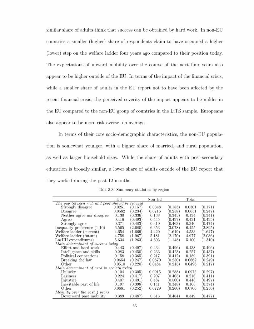
similar share of adults think that success can be obtained by hard work. In non-EU

countries a smaller (higher) share of respondents claim to have occupied a higher

(lower) step on the welfare ladder four years ago compared to their position today.

The expectations of upward mobility over the course of the next four years also

appear to be higher outside of the EU. In terms of the impact of the financial crisis,

while a smaller share of adults in the EU report not to have been affected by the

recent financial crisis, the perceived severity of the impact appears to be milder in

the EU compared to the non-EU group of countries in the LiTS sample. Europeans

also appear to be more risk averse, on average.

In terms of their core socio-demographic characteristics, the non-EU popula-

tion is somewhat younger, with a higher share of married, and rural population,

as well as larger household sizes. While the share of adults with post-secondary

education is broadly similar, a lower share of adults outside of the EU report that

they worked during the past 12 months.

Tab. 3.3: Summary statistics by region

EU Non-EU TotalThe gap between rich and poor should be reduced

Strongly disagree 0.0251 (0.157) 0.0348 (0.183) 0.0301 (0.171)Disagree 0.0582 (0.234) 0.0716 (0.258) 0.0651 (0.247)Neither agree nor disagree 0.130 (0.336) 0.138 (0.345) 0.134 (0.341)Agree 0.416 (0.493) 0.445 (0.497) 0.431 (0.495)Strongly agree 0.371 (0.483) 0.310 (0.463) 0.340 (0.474)

Inequality preference (1-10) 6.565 (2.680) 6.353 (3.078) 6.455 (2.895)Welfare ladder (current) 4.654 (1.669) 4.420 (1.619) 4.533 (1.647)Welfare ladder (future) 4.758 (1.967) 5.181 (2.170) 4.977 (2.086)Ln(HH expenditures) 5.634 (1.263) 4.603 (1.148) 5.100 (1.310)Main determinant of success today

Effort and hard work 0.443 (0.497) 0.434 (0.496) 0.438 (0.496)Intelligence and skills 0.283 (0.450) 0.233 (0.423) 0.257 (0.437)Political connections 0.158 (0.365) 0.217 (0.412) 0.189 (0.391)Breaking the law 0.0654 (0.247) 0.0670 (0.250) 0.0662 (0.249)Other 0.0510 (0.220) 0.0484 (0.215) 0.0496 (0.217)

Main determinant of need in society todayUnlucky 0.104 (0.305) 0.0915 (0.288) 0.0975 (0.297)Laziness 0.224 (0.417) 0.207 (0.405) 0.216 (0.411)Injustice 0.407 (0.491) 0.487 (0.500) 0.448 (0.497)Inevitable part of life 0.197 (0.398) 0.141 (0.348) 0.168 (0.374)Other 0.0681 (0.252) 0.0729 (0.260) 0.0706 (0.256)

Mobility over the past 4 yearsDownward past mobility 0.389 (0.487) 0.313 (0.464) 0.349 (0.477)

63

No past mobility 0.418 (0.493) 0.422 (0.494) 0.420 (0.494)Upward past mobility 0.193 (0.395) 0.265 (0.442) 0.231 (0.421)

How much were you impacted by the financial crisis?A great deal 0.139 (0.346) 0.197 (0.398) 0.169 (0.375)A fair amount 0.267 (0.443) 0.269 (0.443) 0.268 (0.443)Just a little 0.308 (0.462) 0.174 (0.379) 0.239 (0.426)Not at all 0.261 (0.439) 0.291 (0.454) 0.276 (0.447)Don’t know 0.0248 (0.155) 0.0694 (0.254) 0.0479 (0.213)

Risk aversion hypotheticalWould take the risk 0.339 (0.473) 0.354 (0.478) 0.347 (0.476)Would not take the risk 0.570 (0.495) 0.473 (0.499) 0.520 (0.500)Don’t know 0.0917 (0.289) 0.173 (0.378) 0.134 (0.341)

Age 49.03 (17.15) 43.18 (16.72) 46.01 (17.18)Female 0.586 (0.493) 0.605 (0.489) 0.596 (0.491)University education 0.216 (0.412) 0.198 (0.398) 0.207 (0.405)Employed 0.557 (0.497) 0.477 (0.499) 0.515 (0.500)Ln(HH size) 0.752 (0.536) 1.107 (0.574) 0.936 (0.584)Household composition

Children’s share in HH 0.115 (0.197) 0.165 (0.212) 0.141 (0.207)Female share in HH 0.538 (0.295) 0.530 (0.242) 0.534 (0.269)Elderly share in HH 0.144 (0.314) 0.0736 (0.231) 0.108 (0.277)

Market is preferred 0.343 (0.475) 0.380 (0.485) 0.362 (0.481)Non-Orthodox 0.856 (0.351) 0.516 (0.500) 0.680 (0.466)Not married 0.465 (0.499) 0.363 (0.481) 0.412 (0.492)Rural 0.343 (0.475) 0.447 (0.497) 0.396 (0.489)Observations 13679 14671 28350Note: Mean of each variable with standard deviation in parentheses.

3.4 Main results and robustness checks

3.4.1 Main results

The estimates for the baseline specification for the whole region are presented

in Table 3.4. Column (1) reports estimates for the whole sample, column (2) reports

the estimates for the same model estimated among those with a low degree of risk

aversion (those who said that they would take the risk in the hypothetical scenario),

and column (3) reports estimates for the risk averse sub-sample. Among those with

a low degree of risk aversion and relative to the group of respondents who are above

average today and expect to remain so four years hence (Group 4) the respondents

who are below average today and expect to remain so in the future (Group 1)

exhibit a higher preference for reducing the gap between the rich and the poor in

their country, whereas the redistributive preferences of the POUM group are not

statistically different from those of Group 4 (i.e. the null hypothesis β2 = 0 is not

64

rejected). It is also the case that β1 − β2 > 0, as required in the present setup

for the POUM hypothesis not to be rejected. These findings are in contrast to the

estimates for the risk-averse sample, where the POUM group together with the stable

low group are more likely than the stable above average group to support a smaller

gap between the rich and the poor. Furthermore, β1 − β2 = 0 cannot be rejected in

the risk-averse sub-sample. The estimates from the low risk aversion sub-sample and

the high risk aversion sub-sample, viewed together, are consistent with the POUM

hypothesis put forth by Benabou and Ok (2001). The fact that estimates in the

overall sample that does not differentiate according to the degree of risk aversion

reject the POUM hypothesis (on account of β2 > 0) highlights the importance of

accounting for risk aversion in empirical tests of the POUM hypothesis, something

existing studies based on observational data have been unable to do.

The other estimates in Table 3.4 are consistent with findings in existing stud-

ies. Consistent with the reasoning in Piketty (1995), beliefs about the importance of

effort figure prominently into redistributive preferences irrespective of one’s degree

of risk aversion. Respondents who believe that success is mainly driven by politi-

cal connections or by breaking the law (relative to the reference category of effort

and hard work) are more supportive of reducing the gap between the rich and the

poor, while those who believe success to be driven by intelligence and skills are less

supportive. If need in society is perceived to be the result of injustice, this is asso-

ciated with greater preference for redistribution, whereas the opposite is true when

need is viewed as driven by laziness. Past upward mobility is negatively associated

with the support for bridging the gap between the rich and the poor in the low risk

65

Tab. 3.4: POUM Hypothesis - Baseline

Overall Risk loving Risk averse

Group 1 (β1) 0.205*** 0.269*** 0.229***(0.039) (0.059) (0.048)

Group 2 (β2) 0.102** 0.085 0.158***(0.049) (0.076) (0.061)

Group 3 (β3) 0.051 0.032 0.090(0.044) (0.072) (0.056)

Success due to: effort and hard work ref. ref. ref.Intelligence and skills -0.093*** -0.154*** -0.078*

(0.034) (0.052) (0.044)Political connections 0.179*** 0.162** 0.175***

(0.051) (0.073) (0.065)Breaking the law 0.219*** 0.229** 0.201**

(0.066) (0.096) (0.088)Other 0.155** 0.114 0.299***

(0.064) (0.109) (0.088)Need due to: inevitable part of life ref. ref. ref.Unlucky -0.059 -0.081 -0.011

(0.049) (0.078) (0.065)Laziness -0.099** -0.133** -0.080

(0.043) (0.067) (0.055)Injustice 0.265*** 0.196*** 0.294***

(0.041) (0.064) (0.052)Other -0.058 -0.131 0.053

(0.066) (0.107) (0.079)Market preferred -0.144*** -0.094* -0.218***

(0.034) (0.049) (0.045)No past mobility ref. ref. ref.Downward past mobility 0.042 0.010 0.076*

(0.036) (0.057) (0.043)Upward past mobility -0.038 -0.117* 0.006

(0.038) (0.060) (0.049)

Pseudo R-squared 0.031 0.036 0.037Obs 28350 9826 14729β1 - β2 0.103 0.183 0.071Prob>chi2 0.039 0.017 0.269

Notes: Ordered logit regressions. Robust standard errors, clustered at primary sampling unit level inparentheses. Regressions also include the following set of controls: Ln(HH expenditures), crisis impact,age and age squared, sex, education, Ln(HH size), household composition, religion, marital status, area ofresidence and country dummies. Significance: * p<0.10, ** p<0.05, *** p<0.01.

66

aversion sub-sample, but not among the risk averse respondents. For them it is past

downward mobility that matters. Ideology also matters, confirming earlier results

by Alesina and Giuliano (2009). Those who think that a market economy is always

the preferred economic system are less supportive of reducing the gap between the

rich and the poor, especially if they are also risk averse.

Other estimates, not reported to conserve space, suggest that the preference

for redistribution increases concavely with age and is lower among those with a post-

secondary level of education. Given that the data was collected in the aftermath

of the recent financial crisis, it is not surprising that those who were affected more

by the crisis are also more supportive of bridging the gap between the rich and the

poor, irrespective of their degree of risk aversion.

The same empirical models are re-estimated separately for EU-member coun-

tries and non-EU countries in the sample to explore whether similar patterns can

be found in both groups. In both cases estimates are presented separately for the

low risk aversion respondents and the high risk aversion respondents (Table 3.5).

In the European Union the results are substantively similar to those for the over-

all sample. The data again support the POUM hypothesis – prospects of upward

mobility combined with a low degree or risk aversion are associated with a lower

preference for bridging the gap between the rich and the poor, whereas a high degree

of risk aversion makes redistributive preferences stronger, such that they are similar

to those held by those who see themselves as being in the bottom half of the welfare

distribution and expect to remain there in the future.

Beliefs about the determinants of success and need, and in particular the

67

Tab. 3.5: POUM Hypothesis: EU and non-EU countries

EU Non-EURisk loving Risk averse Risk loving Risk averse

Group 1 (β1) 0.368*** 0.298*** 0.157* 0.117(0.085) (0.061) (0.083) (0.076)

Group 2 (β2) 0.177 0.234*** 0.026 0.067(0.117) (0.084) (0.101) (0.090)

Group 3 (β3) 0.164* 0.132* -0.103 0.033(0.096) (0.079) (0.105) (0.079)

Success due to: effort and hard work ref. ref. ref. ref.Intelligence and skills -0.197*** -0.029 -0.112 -0.138*

(0.072) (0.053) (0.075) (0.073)Political connections 0.156 0.317*** 0.148 0.047

(0.108) (0.083) (0.101) (0.098)Breaking the law 0.349*** 0.309** 0.097 0.085

(0.127) (0.132) (0.141) (0.122)Other 0.122 0.376*** 0.091 0.219

(0.157) (0.114) (0.151) (0.134)Need due to: inevitable part of life ref. ref. ref. ref.Unlucky -0.054 -0.048 -0.110 -0.002

(0.104) (0.083) (0.118) (0.104)Laziness -0.095 -0.170** -0.151 -0.019

(0.090) (0.070) (0.101) (0.089)Injustice 0.353*** 0.440*** 0.036 0.099

(0.088) (0.067) (0.093) (0.079)Other 0.110 0.083 -0.322** -0.011

(0.146) (0.103) (0.152) (0.125)Market preferred -0.204*** -0.384*** 0.007 -0.027

(0.066) (0.057) (0.069) (0.067)No past mobility ref. ref. ref. ref.Downward past mobility 0.130* 0.141** -0.135* -0.028

(0.079) (0.056) (0.082) (0.068)Upward past mobility -0.082 0.016 -0.165** -0.032

(0.083) (0.063) (0.084) (0.074)

Pseudo R-squared 0.048 0.047 0.027 0.033Obs 4634 7791 5192 6938β1 - β2 0.191 0.065 0.131 0.050Prob>chi2 0.098 0.456 0.205 0.602

Notes: Ordered logit regressions. Robust standard errors, clustered at primary sampling unit level inparentheses. Regressions also include the following set of controls: Ln(HH expenditures), crisis impact,age and age squared, sex, education, Ln(HH size), household composition, religion, marital status, area ofresidence and country dummies. Significance: * p<0.10, ** p<0.05, *** p<0.01.

68

importance of political connections for success and of injustice as a primary driver

of need in society are associated with preferences for greater redistribution even

when the degree of risk aversion is low. Ideological preferences, captured here by

the belief in the superiority of the market economy in all circumstances, have the

opposite effect. Unlike in the overall sample, downward past mobility is associated

with stronger redistributive preferences in the EU countries.

The estimates from non-EU countries, on the other hand, stand in sharp con-

trast to the above findings. Here the POUM hypothesis is not borne out by the data.

Whereas β2 = 0 cannot be rejected, the preference for reducing the gap between the

rich and the poor in the POUM group does not appear to be statistically lower than

in Group 1 in the low risk aversion sub-sample (the null hypothesis β1 − β2 = 0

cannot be rejected).

Other drivers of redistributive preferences that proved to be important in the

EU do not appear to matter in non-EU countries, although the relationship between

redistributive preferences and variables such as age, sex and education are qualita-

tively similar. In particular, the perceived importance of political connections for

success, or of injustice for poverty, are not associated with a stronger desire to reduce

the gap between the rich and the poor, and the preference for markets is similarly

not significant. In the low risk aversion sub-sample, both upward past mobility is

negatively associated with preferences for more redistribution (perhaps to protect

some of the gains). It is the case, however, that the stronger impact of the financial

crisis is still associated with a preference for more redistribution, as was the case in

the EU group.

69

Lack of dynamic considerations among determinants of redistributive prefer-

ences outside of the European Union is more general than the restricted sense of

the prospects of upward mobility suggested by Benabou and Ok (2001) and tested

above. If instead redistributive preferences are re-estimated as a function of the cur-

rent economic ladder and of the future economic ladder (not reported to conserve

space), a higher position on the current economic ladder is negatively associated with

the preference for reducing the gap between the rich and the poor, whereas the po-

sition on the future economic ladder is insignificant both among the risk averse and

the risk loving respondents. It is plausible that the greater political and economic

uncertainty outside of the EU makes it more difficult to link current preferences

with expectations of the future, or to believe in medium-term policy stability, as the

POUM model requires.

The reasons why beliefs about whether effort or connections determine success

(or whether luck or injustice determine need) in society are associated with greater

preference for redistribution in the EU countries but not outside of the EU are sim-

ilarly difficult to uncover with the LiTS data. One plausible explanation, however,

is that outside of the European Union inequality of opportunity is more widespread

and this leads people to adapt to it, which attenuates the link between perceptions

of unfairness and preferences for redistribution. Graham (2010) suggests, for in-

stance, that well-being effects of corruption have been found to be lower for those

living in countries where corruption is the status quo and people are accustomed

to it. Related to this, Graham and Chattopadhyay (2009) find that the wellbeing

effects of crime are lower when crime is widespread. I return briefly to this question

70

in section 3.5.

3.4.2 Robustness analysis

As a robustness check, I re-estimate the baseline model with an alterna-

tive proxy for redistributive preferences. In addition to reporting their opinion

on whether “the gap between the rich and the poor should be reduced” the sur-

vey questionnaire also elicits respondents’ views on inequality based on a 1-10 scale

where 1 corresponds to the statement “incomes should be made more equal” and 10

corresponds to the statement “we need larger income differences as incentives for

individual effort”. Respondents are asked to report 1 if they completely agree with

the former statement, 10 if they completely agree with the latter statement, and

to choose any number in between if their views fall somewhere in between the two

statements. To make the estimates consistent with the earlier results, the scale is

reversed such that complete agreement with the statement “we need larger income

differences as incentives for individual effort” is recoded as 1, and compete agree-

ment with the statement “incomes should be made more equal” is correspondingly

recoded as 10, and a positive coefficient on an independent variable implies higher

preference for redistribution associated with it. The estimates of the model with this

alternative dependent variable (Table 3.6) confirm the predictions of the the POUM

hypothesis for the group of European Union countries. In the non-EU countries

the POUM hypothesis is not borne out by the data, similarly to the results of the

baseline model.

A further robustness check could be performed by specifying an artificially low

threshold that defines the future mobility groups. Table 3.7 reports the estimates for

71

Tab. 3.6: POUM Hypothesis - Alternative inequality preference


β1 0.458*** 0.322*** 0.180** 0.324***(0.081) (0.064) (0.081) (0.075)

β2 0.053 0.197** 0.025 0.130(0.108) (0.078) (0.097) (0.101)

β3 0.251*** 0.058 0.066 0.188**(0.097) (0.084) (0.098) (0.089)


Notes: Ordered logit regressions. Robust standard errors, clustered at primary sampling unit level inparentheses. Regressions include the same full set of controls like the baseline model. Significance: * 0.05** 0.01 *** 0.001.

the the EU and non-EU groups of countries, where the rung 3 of the welfare ladder

is taken as the threshold that separates the “above average” group from the “below

average” group. Thus, the POUM group is composed of those who are on rung 1 or

2 of the welfare ladder currently but believe that they will be on rung 3 or above

in the future. The other three groups are correspondingly defined as being on one

side of this threshold in both years, or moving down across this threshold (Group 3).

Arguably, moving up from rung 1 or 2 to rung 3 or even 4 is still far from being“above

average”. Such respondents would still remain rather low on the welfare ladder, even

if upwardly mobile, and as such, should still have strong redistributive preferences.

As the result, one would not expect to find support for the POUM hypothesis with

this artificially low threshold. This intuition is confirmed by the estimates in Table

3.7. Even in the EU sample, where support for the POUM hypothesis was found in

the analysis above, the hypothesis β1 − β2 = 0 can never be rejected, even in the

low risk aversion sub-sample. Also, β2 = 0 in the high risk aversion group but not

in the low risk aversion group, which is counter-intuitive.

72

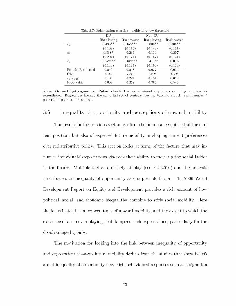
Tab. 3.7: Falsification exercise - artificially low threshold


β1 0.496** 0.458*** 0.300** 0.306**(0.193) (0.116) (0.143) (0.131)

β2 0.388* 0.236 0.119 0.207(0.207) (0.171) (0.157) (0.131)

β3 0.652*** 0.489*** 0.417** 0.078(0.140) (0.121) (0.190) (0.124)


Notes: Ordered logit regressions. Robust standard errors, clustered at primary sampling unit level inparentheses. Regressions include the same full set of controls like the baseline model. Significance: *p<0.10, ** p<0.05, *** p<0.01.

3.5 Inequality of opportunity and perceptions of upward mobility

The results in the previous section confirm the importance not just of the cur-

rent position, but also of expected future mobility in shaping current preferences

over redistributive policy. This section looks at some of the factors that may in-

fluence individuals’ expectations vis-a-vis their ability to move up the social ladder

in the future. Multiple factors are likely at play (see EU 2010) and the analysis

here focuses on inequality of opportunity as one possible factor. The 2006 World

Development Report on Equity and Development provides a rich account of how

political, social, and economic inequalities combine to stifle social mobility. Here

the focus instead is on expectations of upward mobility, and the extent to which the

existence of an uneven playing field dampens such expectations, particularly for the

disadvantaged groups.

The motivation for looking into the link between inequality of opportunity

and expectations vis-a-vis future mobility derives from the studies that show beliefs

about inequality of opportunity may elicit behavioural responses such as resignation

73

and reduced ambition, which can lead to inequality traps (for a discussion, see World

Bank 2005; Bourguignon et al. 2006). For instance, Appadurai (2004) argues that

deprivation can reduce the “capacity to aspire” and, hence, effort. In the theoretical

model proposed by Piketty (1995) prior beliefs about the existence of inequality of

opportunity translate into low effort, which in turn leads to poor outcomes, but, due

to dynastic learning, the bad outcomes only reinforce the prior beliefs. Experimental

work in India suggests that children from low castes perform tasks such as solving

a maze better when not reminded of their caste (Hoff and Pandey, 2006). One may

be less determined to invest in education, when jobs are obtained primarily through

connections.

To assess the extent to which a level playing field exists I rely on the respon-

dents’ assessments of the importance of “having connections” in order to progress in

a number of crucial dimensions of life, based on the following set of questions: “Some

people, because of their job, position in the community or contacts, are asked by

others to help influence decisions in their favour. In general, how important is it in

our country to have the support of such people to influence decisions in the following

situations?” The following domains of life are considered in the survey: (i) to get

a good job in the government sector; (ii) to get a good job in the private sector;

(iii) to get into university; (iv) to settle a dispute with a neighbour; (v) to obtain

permits or official papers. The respondents could choose from the following options:

not important at all, somewhat important, moderately important, very important,

and essential. Only 3 percent of respondents in the pooled sample think that con-

nections are not important at all, such that there appears to be a universal belief

74

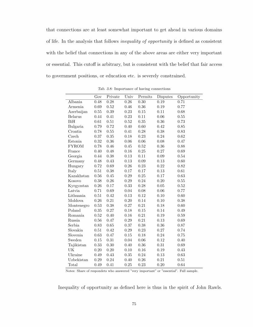
that connections are at least somewhat important to get ahead in various domains

of life. In the analysis that follows inequality of opportunity is defined as consistent

with the belief that connections in any of the above areas are either very important

or essential. This cutoff is arbitrary, but is consistent with the belief that fair access

to government positions, or education etc. is severely constrained.

Tab. 3.8: Importance of having connections

Gov Private Univ Permits Disputes OpportunityAlbania 0.48 0.28 0.26 0.30 0.19 0.71Armenia 0.69 0.52 0.46 0.36 0.19 0.77Azerbaijan 0.55 0.39 0.23 0.15 0.11 0.68Belarus 0.44 0.41 0.23 0.11 0.06 0.55BiH 0.61 0.51 0.52 0.35 0.36 0.73Bulgaria 0.79 0.72 0.40 0.60 0.42 0.85Croatia 0.78 0.55 0.41 0.28 0.38 0.83Czech 0.37 0.35 0.18 0.23 0.24 0.62Estonia 0.32 0.36 0.06 0.06 0.08 0.47FYROM 0.78 0.46 0.45 0.52 0.36 0.88France 0.40 0.48 0.16 0.25 0.27 0.69Georgia 0.44 0.38 0.13 0.11 0.09 0.54Germany 0.48 0.43 0.13 0.09 0.13 0.60Hungary 0.72 0.69 0.26 0.23 0.22 0.82Italy 0.51 0.38 0.17 0.17 0.13 0.61Kazakhstan 0.56 0.45 0.29 0.25 0.17 0.63Kosovo 0.38 0.26 0.29 0.24 0.20 0.55Kyrgyzstan 0.26 0.17 0.33 0.28 0.05 0.52Latvia 0.71 0.69 0.04 0.08 0.06 0.77Lithuania 0.51 0.42 0.13 0.12 0.10 0.60Moldova 0.26 0.21 0.20 0.14 0.10 0.38Montenegro 0.53 0.38 0.27 0.21 0.18 0.60Poland 0.35 0.27 0.18 0.15 0.14 0.49Romania 0.52 0.40 0.16 0.21 0.19 0.59Russia 0.56 0.47 0.29 0.21 0.13 0.69Serbia 0.83 0.65 0.37 0.38 0.36 0.87Slovakia 0.51 0.42 0.29 0.23 0.27 0.74Slovenia 0.63 0.47 0.15 0.18 0.24 0.75Sweden 0.15 0.31 0.04 0.06 0.12 0.40Tajikistan 0.33 0.30 0.40 0.36 0.31 0.69UK 0.20 0.20 0.10 0.16 0.19 0.43Ukraine 0.49 0.43 0.35 0.24 0.13 0.63Uzbekistan 0.29 0.24 0.40 0.26 0.21 0.51Total 0.49 0.41 0.25 0.23 0.20 0.64

Notes: Share of respondets who answered ”very important” or ”essential”. Full sample.

Inequality of opportunity as defined here is thus in the spirit of John Rawls.

75

Recall that the second part of the Second Principle of Justice proposed by Rawls

(1971) requires that offices and positions in society are open to all on a fair basis.7

This is precisely what is queried by the above survey questions, since need for

connections to get jobs in various sectors, or to get necessary permits for business

activity is in direct contradiction of the Second Principle as it denies equal access

to all.

The perceptions of inequality of opportunity are quite widespread in the region.

For instance, almost half of the adults in the region believe that it is very important

or essential to have connections to get a good government job, in Croatia and in

FYROM the share exceeds three quarters, and in Serbia it is greater than 80 percent.

On the other hand, in the UK and in Sweden no more than 20 percent of adults

share this view. In some of the Transition countries the need for connections to get

a good public sector job is also perceived to be low, such as in Estonia, Kyrgyzstan,

Moldova, Tajikistan and Uzbekistan where less than one third of adults believe that

connections are very important or essential for public sector jobs. The need for

connections is generally perceived to be lower in other domains of life, although

the share of adults who believe that connections are necessary in these other areas

remains non-trivial in most countries (Table 3.8).8

The first part of Rawls’s Second Principle of Justice allows for inequalities to

exist to the extent that they are to the greatest benefit of the least advantaged.

This is not the case in practice. In the LiTS survey the respondents are further

7 The two principles of justice proposed by Rawls are as follows: First Principle - “each person is to have anequal right to the most extensive total system of equal basic liberties compatible with a similar system of libertyfor all”; and Second Principle - “Social and economic inequalities are to be arranged so that they are both: (a) tothe greatest benefit of the least advantaged, consistent with the just savings principle, and (b) attached to officesand positions open to all under conditions of fair equality of opportunity.” (Rawls, 1971: p.302).

8 The last column in Table 3.8 is our measure of inequality of opportunity, which, for each individual evaluatesto 1 if connections in any of the five areas are very important or essential, and zero otherwise.

76

asked if they knew of anyone (friends, relatives, classmates, local boss, etc.) who

could influence decisions with respect to getting a good government job, or getting

into university etc., should such influence be needed. Overall in the LiTS survey 32

percent of the adult population reported that they do not know any such person,

but this share is generally higher for individuals who place themselves at the bottom

of the welfare ladder, or those who (or whose parents) had low levels of education.

It is perhaps not surprising that disadvantaged groups are least likely to thrive in

the presence of inequality of opportunity. These two characteristics – the impor-

tance of connections to get ahead and lack of such connections – combine to create

what Bourguignon et al. (2006) call “inequality traps” or the persistence of relative

positions (and implicitly of poverty and vulnerability) over time.

3.5.1 Empirical strategy

In order to investigate whether inequality of opportunity dampens expectations

of future mobility, a relationship similar to the one used to test the POUM hypothesis

is estimated:

Statusf∗i = δ1Conn1i + δ2Conn

2i + δ3Conn

3i +X

′iγ + εi,

where Statusf∗i is the latent future economic status, it is assumed that the observed

expected future economic status Statusfi = k if µk−1 ≤ Statusf∗i < µk, where µk are

unknown cut points with µ0 = −∞ and µ10 = ∞. Connji dummies represent the

intersection of the respondent’s view on the importance of connections (either vital or

not, where vital is defined as very important or essential) and whether the respondent

has such connections or not. This interaction creates four categories, namely: (i)

77

connections are not vital but available (reference category); (ii) connections are not

vital and not available (Conn1i ); (iii) connections are vital and available (Conn2

i );

and (iv) connections are vital and not available (Conn3i ).

It is hypothesised that perceptions of an uneven playing field, when they are

combined with lack of informal connections to overcome these, will have a dampening

effect on expectations of future mobility, or δ3 < 0. Two additional hypotheses are

tested:

• δ2−δ3 > 0, i.e. when the playing field is not even, connections improve prospects

of future upward mobility;

• δ1− δ3 > 0, i.e. if connections are unavailable, inequality of opportunity damp-

ens prospects of future upward mobility.

A number of important confounding factors need to be accounted for in the model,

and are included in the Xi vector. Factors such as the person’s education and em-

ployment status have been shown to have a strong effect on social mobility (Bozeat et

al. 2010). The respondent’s age is included to account for the fact that there may be

greater scope for younger individuals to move up the ladder in the future, compared

to those who are nearing retirement. Similarly, the respondent’s sex and religious af-

filiation are included to account for possible differences in ambition between men and

women, or across religious denominations, which may lead to different aspirations

for the future.

It is the case the respondents who are currently at the top of the current

welfare ladder have less scope of moving up the ladder, and similarly those at the

bottom are less likely to move lower still in the near future. Moreover, the current

78

position on the welfare ladder can be correlated with the person’s assessment of the

importance of having connections to succeed in the labour market or in terms of

education. For this reason, I control for the respondent’s current position on the

welfare ladder in all specifications in this section. In addition, the individual’s past

mobility experience may influence future expectations. It is difficult to say a priori

how past experience may translate into future expectations. It may be, for instance,

that past upward (downward) mobility may indicate further upward (downward)

mobility in the future. It is also possible, however, that upward (downward) mobility

in the past leaves less scope for further upward (downward) mobility in the future.

The direction of the effect is likely to depend on other characteristics of the individual

and is investigated empirically by including dummies indicating either upward or

downward past mobility (no past mobility being the reference category).

Expectations of future mobility may similarly be influenced by the recent fi-

nancial crisis experience. Those who were affected by the crisis but believe its impact

to be transitory may expect to move up the ladder in the next four years as part

of regaining the lost status due to the crisis. It is similarly possible that those who

were strongly affected by the crisis in a way that is not easy to recover from over

the short term may have modest expectations of upward mobility in the future. To

account for such confounding effects, I also control for the respondent’s assessment

of the degree to which she have been affected by the financial crisis.

As in the case of the POUM hypothesis, it is important to account for the

individual’s degree of risk aversion, since those who are less risk averse may be more

likely to engage in risky projects and expect to to move up the ladder based on

79

their belief of their success. Risk averse individuals, on the other hand, may be

more likely to prefer stability, which in turn may lead to expectations of the stable

position on the society’s welfare ladder in the future. To account for the individual’s

degree of risk aversion I include dummies based on the hypothetical drought scenario

described in section 3.2.2.

The literature on inequality of opportunity generally distinguishes between

inequality due to unequal opportunities, and inequality due to effort (Bourguignon

et al. 2003; Roemer et al. 2003; Ooghe et al. 2007; Checchi and Peragine 2009;

Cogneau and Mesple-Somps 2008; Ferreira and Gignoux 2008; Ferreira et al. 2008,

2010). However, as noted by Lefranc et al. (2009), luck is also an important factor,

but generally gets bundled together with effort. In the LiTS survey it is possible

to account for the influence of luck by conditioning on the individual’s beliefs with

regard to the reasons why there are people in need in society, whether it be luck,

laziness, an inevitable part of modern life, or injustice in society.

Included in the Xi vector are also country dummies, such that estimates rely

on within-country variation. The full set of controls, which also includes household

size and composition, is listed in Table 3.3. As before, ordered logistic regressions

are estimated, and errors are allowed to be correlated within primary sampling units.

3.5.2 Results

Column (1) of table 3.9 presents the estimates of ordered logistic regressions for

the whole LiTS sample. First, δ3 < 0, such that inequality of opportunity coupled

with lack of connections is negatively associated with prospects of future mobility.

Second, when there is inequality of opportunity, connections matter (δ2 − δ3 > 0)

80

and lack thereof is associated with expectations of a lower position on the future

social ladder. The reasons why δ2 may be negative I return to below.

It is also the case that lack of connections matters δ1 < 0, even when they

are not perceived to be vital. To understand why this may be the case, recall that

here when connections are “not vital”, they need not be “not important at all”,

rather, they can be somewhat or moderately important. Therefore, the distinction

here is between severe inequality of opportunity and mild inequality of opportunity,

since very few respondents perceive opportunities to be equal in the “connections

are not important at all” sense. More importantly, however, δ1 − δ3 > 0, i.e. when

connections are unavailable, the extent of IO matters.

The same specification is re-estimated for the European Union countries (col-

umn 2) and non-EU countries (column 3). In the non-EU sample the results are

similar in the sense that when there is inequality of opportunity, it helps to have

connections (δ2− δ3 > 0), and when connections are unavailable, it matters whether

the playing field is level or not (δ1 − δ3 > 0).

One of the key difference in the group of EU countries is that when there is

inequality of opportunity, there appears to be no difference between having connec-

tions and not having connections (δ2 − δ3 = 0 cannot be rejected). One possible

reason for this difference could be due to the fact that it may be less common -

and possibly less socially acceptable - to rely on informal connections in the Eu-

ropean Union. One would certainly expect reliance on informal institutions to be

more prevalent when formal institutions are weaker. There is some evidence in the

LiTS survey that supports this reasoning. The respondents who claimed to have

81

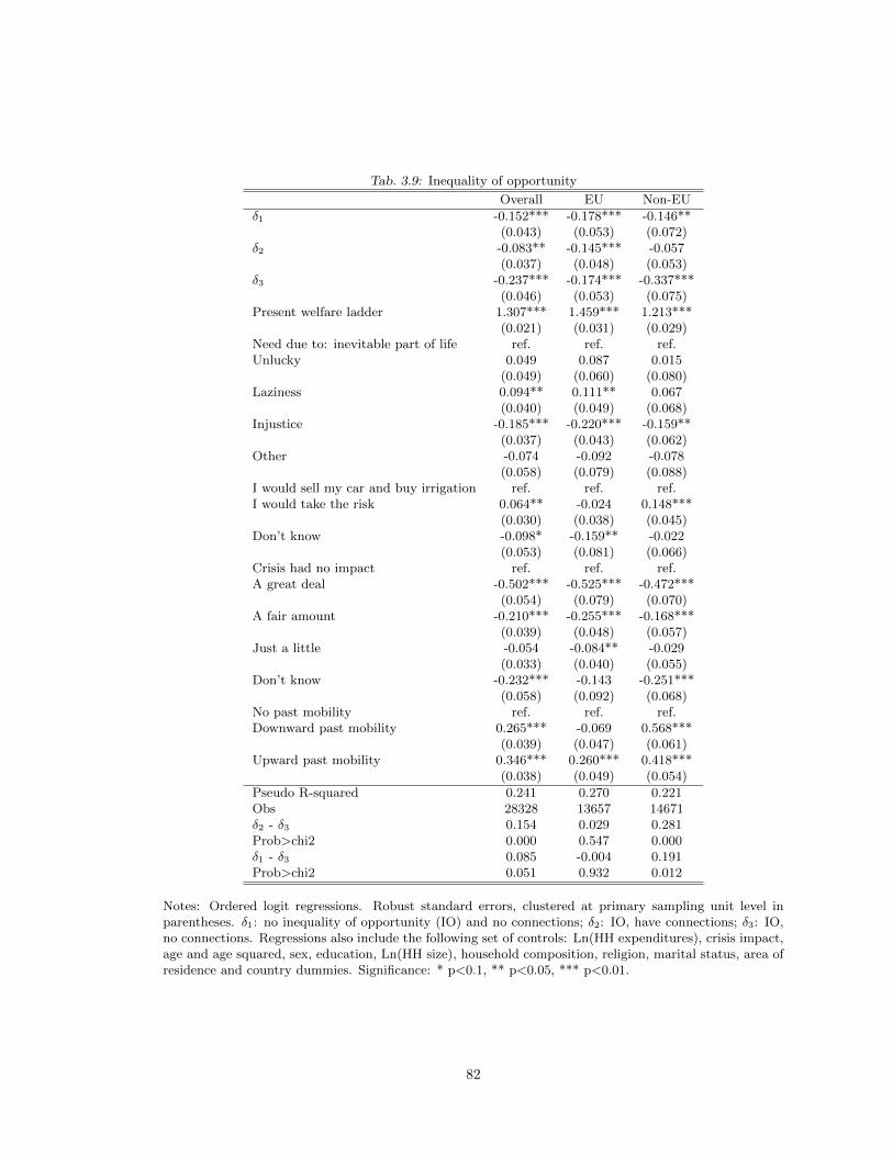
Tab. 3.9: Inequality of opportunity

Overall EU Non-EU

δ1 -0.152*** -0.178*** -0.146**(0.043) (0.053) (0.072)

δ2 -0.083** -0.145*** -0.057(0.037) (0.048) (0.053)

δ3 -0.237*** -0.174*** -0.337***(0.046) (0.053) (0.075)

Present welfare ladder 1.307*** 1.459*** 1.213***(0.021) (0.031) (0.029)

Need due to: inevitable part of life ref. ref. ref.Unlucky 0.049 0.087 0.015

(0.049) (0.060) (0.080)Laziness 0.094** 0.111** 0.067

(0.040) (0.049) (0.068)Injustice -0.185*** -0.220*** -0.159**

(0.037) (0.043) (0.062)Other -0.074 -0.092 -0.078

(0.058) (0.079) (0.088)I would sell my car and buy irrigation ref. ref. ref.I would take the risk 0.064** -0.024 0.148***

(0.030) (0.038) (0.045)Don’t know -0.098* -0.159** -0.022

(0.053) (0.081) (0.066)Crisis had no impact ref. ref. ref.A great deal -0.502*** -0.525*** -0.472***

(0.054) (0.079) (0.070)A fair amount -0.210*** -0.255*** -0.168***

(0.039) (0.048) (0.057)Just a little -0.054 -0.084** -0.029

(0.033) (0.040) (0.055)Don’t know -0.232*** -0.143 -0.251***

(0.058) (0.092) (0.068)No past mobility ref. ref. ref.Downward past mobility 0.265*** -0.069 0.568***

(0.039) (0.047) (0.061)Upward past mobility 0.346*** 0.260*** 0.418***

(0.038) (0.049) (0.054)

Pseudo R-squared 0.241 0.270 0.221Obs 28328 13657 14671δ2 - δ3 0.154 0.029 0.281Prob>chi2 0.000 0.547 0.000δ1 - δ3 0.085 -0.004 0.191Prob>chi2 0.051 0.932 0.012

Notes: Ordered logit regressions. Robust standard errors, clustered at primary sampling unit level inparentheses. δ1: no inequality of opportunity (IO) and no connections; δ2: IO, have connections; δ3: IO,no connections. Regressions also include the following set of controls: Ln(HH expenditures), crisis impact,age and age squared, sex, education, Ln(HH size), household composition, religion, marital status, area ofresidence and country dummies. Significance: * p<0.1, ** p<0.05, *** p<0.01.

82

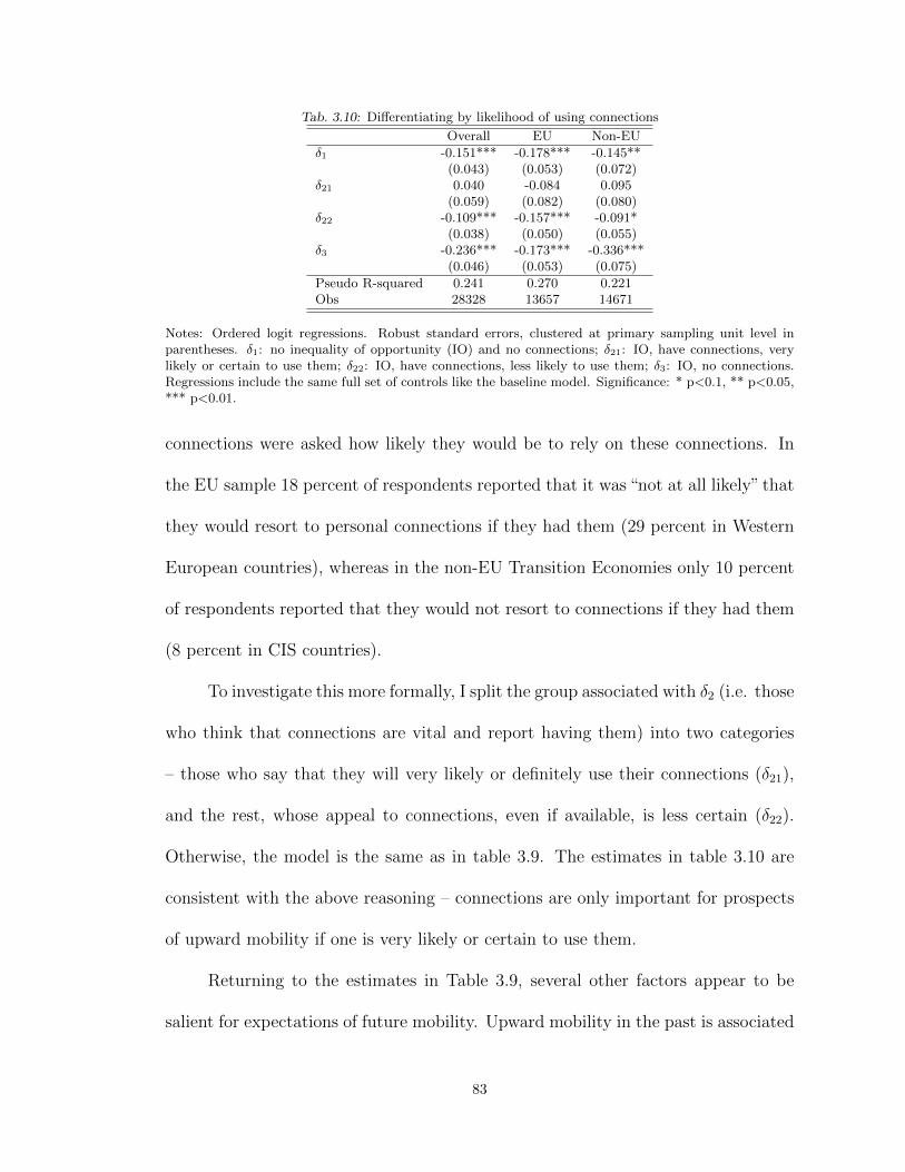
Tab. 3.10: Differentiating by likelihood of using connections

Overall EU Non-EU

δ1 -0.151*** -0.178*** -0.145**(0.043) (0.053) (0.072)

δ21 0.040 -0.084 0.095(0.059) (0.082) (0.080)

δ22 -0.109*** -0.157*** -0.091*(0.038) (0.050) (0.055)

δ3 -0.236*** -0.173*** -0.336***(0.046) (0.053) (0.075)

Pseudo R-squared 0.241 0.270 0.221Obs 28328 13657 14671

Notes: Ordered logit regressions. Robust standard errors, clustered at primary sampling unit level inparentheses. δ1: no inequality of opportunity (IO) and no connections; δ21: IO, have connections, verylikely or certain to use them; δ22: IO, have connections, less likely to use them; δ3: IO, no connections.Regressions include the same full set of controls like the baseline model. Significance: * p<0.1, ** p<0.05,*** p<0.01.

connections were asked how likely they would be to rely on these connections. In

the EU sample 18 percent of respondents reported that it was “not at all likely” that

they would resort to personal connections if they had them (29 percent in Western

European countries), whereas in the non-EU Transition Economies only 10 percent

of respondents reported that they would not resort to connections if they had them

(8 percent in CIS countries).

To investigate this more formally, I split the group associated with δ2 (i.e. those

who think that connections are vital and report having them) into two categories

– those who say that they will very likely or definitely use their connections (δ21),

and the rest, whose appeal to connections, even if available, is less certain (δ22).

Otherwise, the model is the same as in table 3.9. The estimates in table 3.10 are

consistent with the above reasoning – connections are only important for prospects

of upward mobility if one is very likely or certain to use them.

Returning to the estimates in Table 3.9, several other factors appear to be

salient for expectations of future mobility. Upward mobility in the past is associated

83

with expectations of further upward mobility in the future. The same is true of past

downward mobility in non-EU countries, but not in the EU countries, where the

estimated coefficient on the downward past mobility is negative. One interpretation

that is consistent with this difference is that perceptions of downward mobility in

the EU are perceived to be of a less transitory nature. It could be that a more stable

economic environment in the EU may leave less scope for those who perceive to have

moved downward in the past to expect a reversal of their fortunes in the immediate

future. It is not possible, however, to confirm this with the LiTS data. Willingness

to take risks is also positively associated with future mobility expectations outside of

the EU, whereas this is not the case in EU countries. On the other hand, the belief

that need is the product of laziness is positively associated with future mobility

expectations only in the EU.

Some other factors have similar effects in both country groupings. A stronger

effect of the recent financial crisis dampens future mobility expectations. The be-

lief that need in society is the product of injustice (the reference category being

“inevitable part of modern life”) also lowers expectations vis-a-vis future upward

mobility.

The estimates on other variables (not reported to conserve space) suggest that

both in both groups of countries expectations of future upward mobility diminish

with age, are higher in urban areas and for those who are not married. In the EU

they are also higher at higher levels of education, whereas outside of the EU they

are higher for those currently employed (whereas there are no differences across

education levels). Men and women have similar aspirations of upward mobility once

84

Tab. 3.11: Inequality of opportunity and returns to education

Overall EU Non-EU

δ1 0.145*** 0.139** 0.169**(0.045) (0.059) (0.069)

δ2 -0.072** -0.087** -0.064(0.034) (0.041) (0.052)

δ3 0.051 0.082 0.017(0.044) (0.058) (0.065)

Pseudo R-squared 0.241 0.270 0.220Obs 28350 13679 14671δ2 - δ3 -0.122 -0.170 -0.080Prob>chi2 0.001 0.001 0.139δ1 - δ3 0.095 0.057 0.152Prob>chi2 0.054 0.370 0.042

Notes: Ordered logit regressions. Robust standard errors, clustered at primary sampling unit level inparentheses. δ1: no inequality of opportunity (IO) and university education; δ2: IO, no university educa-tion; δ3: IO, university education. Regressions include the same full set of controls like the baseline model.Significance: * p<0.1, ** p<0.05, *** p<0.01.

other characteristics and held beliefs are held constant.

One could also ask whether inequality of opportunity reduces “returns to edu-

cation” in terms of the ability of the latter to improve individual chances of upward

mobility. In order to investigate this question similar specifications are estimated,

except that the dummy variable indicating whether connections are vital is inter-

acted instead with whether the respondent has tertiary education. The estimates

are reported in Table 3.11. First, both in the EU countries and in non-EU countries

tertiary education is associated with higher expectations of future upward mobility

when there exists a level playing field (δ1 > 0). Second, in the pooled sample and in

the EU subsample expectations for the future are lower among those without uni-

versity education when there is IO (δ2 < 0), whereas this is not the case outside of

the EU. Third, in the EU, but not outside of the EU, tertiary education is associated

with higher expectations of future social position when there is IO (δ2−δ3 < 0). One

possible explanation for this, albeit one that is not possible to test with the LiTS

data, lies with the deterioration of the education system in Transition Economies

85

Tab. 3.12: Inequality of opportunity and redistributive preferences

Overall EU Non-EU

δ1 0.127** 0.185*** 0.067(0.056) (0.068) (0.094)

δ2 0.376*** 0.413*** 0.353***(0.044) (0.057) (0.064)

δ3 0.441*** 0.511*** 0.378***(0.053) (0.068) (0.082)

Pseudo R-squared 0.034 0.044 0.026Obs 28328 13657 14671δ2 - δ3 -0.065 -0.099 -0.025Prob>chi2 0.173 0.124 0.725δ1 - δ3 -0.314 -0.327 -0.311Prob>chi2 0.000 0.000 0.001

Notes: Ordered logit regressions. Robust standard errors, clustered at primary sampling unit level inparentheses. δ1: no inequality of opportunity (IO) and no connections; δ2: IO, have connections; δ3: IO,no connections. Regressions include the same full set of controls like the baseline model. Significance: *p<0.1, ** p<0.05, *** p<0.01.

after 1989 and the considerable disconnect between the knowledge taught in the ed-

ucational institutions in Transition Economies and the skills that are in demand in

the labour market, as documented by World Bank (2011). Finally, IO is associated

with lower returns to having university education outside of the EU (δ1 − δ3 > 0),

but not in the EU countries.

Finally, in Table 3.12 I explore whether this “Rawlsian” inequality of opportu-

nity is associated with stronger redistributive preferences. The model is re-estimated

with the preference for reducing the gap between the rich and the poor as the depen-

dent variable, and the δ vector corresponds to the intersection of beliefs about the

importance of connections and whether one has such connections, as in the baseline

model reported in table 3.9. The results suggest that both inside and outside of the

EU the perceived existence of inequality of opportunity is associated with stronger

redistributive preferences (δ2 < 0 and δ3 < 0). Also, (δ1 − δ3 < 0) in both groups of

countries, indicating that when connections are unavailable, IO is associated with a

stronger preference for redistribution.

86


It is the case that people who are currently lower on the society’s welfare ladder

are more in favour of redistribution. The results in this paper suggest, however,

that preferences for redistribution go beyond the present economic position of an

individual. In the European Union individuals in the bottom half of the welfare

ladder today who expect to be in the top half of the ladder in the future (and whose

degree of risk aversion is low) have lower preferences for redistribution than those

who expect to remain in the bottom half of society’s welfare ladder. This finding

supports the POUM hypothesis proposed by Benabou and Ok (2001). Outside of

the EU, on the other hand, data do not support the POUM hypothesis. In these

countries attitudes toward redistribution even among those currently in the bottom

half of the welfare ladder and who expect to remain there are not that different

from the attitudes of those who are currently – and expect to remain – in the top

half of the welfare ladder. Since the POUM model relies on the expectations that

policies set today will persist into future periods, it is plausible that greater policy

volatility severs the link between expectations of future mobility and current policy

preferences.

This paper also looked at the link between inequality of opportunity defined

as the perceived need of connections and expectations of future upward mobility.

Inequality of opportunity is perceived to be widespread outside of the EU, but less

so in the EU countries. Furthermore, inequality of opportunity has a dampening

effect on expectations of future mobility even when such connections are available in

the European Union, if the respondent is reluctant to rely upon them. The data also

87

support the argument that existence of stronger formal institutions (as is the EU

case) makes the reliance on informal institutions less socially acceptable, or in any

case there is less willingness to tap into these informal institutions as compared to

non-EU countries. Unlike informal connections, tertiary education does not appear

to promote greater expectations of upward mobility in non-EU countries when there

is inequality of opportunity, whereas it does so in the European Union. Finally,

inequality of opportunity is also associated with stronger redistributive preferences

in both groups of countries.

88

4 Does relative deprivation matter in developing countries?

4.1 Introduction

One of the prominent explanations for the existence of the Easterlin paradox -

an observation by Easterlin (1974) that despite a strong correlation between income

and happiness within a cross-section, real increases in per capita income over time

do not generally translate into increases in reported levels of happiness - is that in

addition to absolute income, relative income is also an important determinant of

happiness or utility.1 If this is the case, then overall increases in income need not

translate into higher reported life satisfaction, if relative status remains unchanged.

Indeed, a number of recent empirical studies, using data from both OECD and de-

veloping countries, have found reference group income to be an important predictor

of well-being (Clark and Oswald 1996; McBride 2001; Ravallion and Lokshin 2002;

Blanchflower and Oswald 2004; Luttmer 2005; Ferrer-i-Carbonell 2005; Graham and

Felton 2006, Fafchamps and Shilpi 2008).

Preferences for status can have important welfare implications. In developed

countries positional concerns have been shown to lead to longer work hours, reduced

savings, higher indebtedness and bankruptcy rates, longer commutes, higher divorce

rates, higher morbidity (Deaton 2001; Eibner and Evans 2005; Frank 2007 and

references therein). If relative status is indeed a welfare-relevant concern even among

the poor in developing countries, it may drive expenditure and savings patterns

that could increase the longer-term poverty vulnerability of poor households.2 For

instance, positional concerns have been found to drive spending on weddings and1 See Clark et al. (2008) for a comprehensive review of the literature.2 On relative status and well-being in developing countries see Clark and Senik (2011) and references therein.

89

funerals (Brown et al. 2011), with expenses oftentimes financed through blood

donations that carry important health risks (Chen and Zhang, 2009).

In most of the studies that examine the importance of relative status the true

reference group is unknown. Instead, researchers choose a reference group, guided

by certain theoretical considerations, and accounting for data constraints, and then

compute the mean or median income (or expenditures) of the chosen reference group.

The importance of relative status for subjective well-being is then assessed based

on a regression of a self-reported measure of life satisfaction or happiness on own

income or expenditures, as well as on the mean or median income or expenditures of

the reference group, conditional on a set of control variables. A non-zero coefficient

on the reference group welfare variable in regressions of this type is taken to indicate

that subjective well-being is not only a function of own welfare, but also of the the

individual’s welfare relative to that of her reference group.

This paper takes advantage of the 2009 survey implemented by the United

Nations Development Programme (UNDP) in six transition economies, in which the

respondents are asked to evaluate their standard of living (whether worse, same

or better) vis-a-vis the majority of people in their (i) settlement (town / village),

(ii) district, (iii) country. They are also asked to rate their standard of living vis-

a-vis their parents. This makes it possible to explore the importance of relative

deprivation as reported directly by the respondent, rather than being imposed by

the researcher. It also allows us to compare the relative salience of different reference

groups.

A further advantage of the UNDP survey is the availability of the interviewer’s

90

own assessment of the conditions of each respondent’s property and of the respon-

dent’s neighbourhood, ranging from slum to elite in both cases. This is useful

because using respondent-defined relative deprivation helps address issues of rela-

tive status observability and of relevance of a given reference groups, but it does not

eliminate the potential endogeneity arising from the fact that assessments of relative

deprivation and of the satisfaction with the standard of living can both be driven

by unobserved cognitive biases. I rely on the interviewer’s assessment of the relative

deprivation to instrument for the respondent’s self-reported relative deprivation.

The estimates from the pooled sample of all six countries, as well as from

regressions estimated separately for each country, suggest that local relative depri-

vation has a strong negative effect on satisfaction with one’s standard of living, even

when we account for important determinants of satisfaction with the standard of

living, including the respondent’s wealth. This is true even among the poorest Tran-

sition Economies (Tajikistan and Moldova). Moreover, relative deprivation vis-a-vis

neighbours appears to be more salient that relative deprivation vis-a-vis parents.

A brief overview of existing studies that look at the impact of relative status

on well-being is provided in Section 4.2. Section 4.3 describes the data used in the

analysis and provides some descriptive statistics. The salience of various reference

groups is explored in Section 4.4.1, while local relative deprivation, including IV

results are presented in Section 4.4.2. Section 4.5 concludes.

4.2 Existing studies of relative status

A number of different reference group definitions have been employed to date

in the literature that examines the effect of relative status on well-being. Most rel-

91

evant to this analysis are inter-personal reference groups, i.e. groups of individuals

who may be important for social comparisons. At the most general level such refer-

ence groups can be categorized into: (i) reference groups based on a set of ’likeness’

attributes; and (ii) reference groups based on geographic proximity. Clearly, inter-

personal comparisons need not be the only relevant dimension. This paper sidesteps

inter-temporal reference points, which are dealt with in a large literature on adap-

tation (Frederick and Loewenstein, 1999; Frey and Stutzer, 2001; Di Tella et al.,

2003; Di Tella et al., 2010). Senik (2009), for instance, finds comparisons with own

economic situation prior to 1989 to still be an important determinant of subjective

well-being 15 years into the transition process in Eastern Europe.

4.2.1 Reference groups based on ’likeness’

Reference groups based on similar characteristics are grounded analytically in

the social comparison theory proposed by Festinger (1954), who argued that indi-

viduals relied on reference groups to evaluate their abilities and opinions, and that

individuals’ tendency to compare with others was decreasing with the discrepancy

between his/her opinions/abilities and those of others. In other words, individuals

seek to compare their abilities/opinions with others who are perceived to be similar

in relevant dimensions. Goethals and Darley (1977) later build on Festinger’s earlier

work to formulate the related attributes hypothesis that states that people compare

themselves with others who are similar on attributes related to and predictive of the

attribute that is under evaluation.3

Van de Stadt et al. (1985) rely explicitly on the related attributes hypothesis

and construct reference groups on the basis of the education level, age and em-

3 For an overview of the history of the theory of social comparison, see Suls and Wheeler, 2000.

92

ployment status of individuals, using data for two waves of a panel survey of 775

households conducted by the Netherlands Central Bureau of Statistics in 1980 and

1981. Their underlying assumption is that age, education and employment status

are important income generating attributes and as such would be the basis of social

comparison.

McBride (2001), in a study based on 1994 General Social Survey data, con-

structs reference groups based on age cohorts of all those within +/- 5 years from

the respondent. The reference group welfare is then calculated as the mean income

for this group. McBride’s choice of the reference group is based on the view that the

individual “associates most with people of his own age and, as the result, compares

his income to theirs.”

Senik (2004), based on data from the Russian Longitudinal Monitoring Sur-

vey, constructs the reference group income by estimating a first stage regression of

individual’s income as a function of education, years of experience, region, branch,

age, sex, and primary occupation type and then uses the predicted income as a

proxy for the individual’s reference group income. The rationale for this approach,

which is similar to that of Clark and Oswald (1996), who looked at the impact

of relative status on job satisfaction, is to construct an “average pay-off associated

with the productive characteristics of a given individual.” One thing to note about

Senik (2004) is that, unlike most other studies that look ta relative income, it finds

reference group income to exert a positive effect on individual satisfaction, which

the author interprets in the spirit of Hirschman’s “tunnel effect” (Hirschman and

Rothschild, 1973), i.e. the reference group income is treated more like an indication

93

of their own future income, rather than of their inferior relative status.

Ferrer-i-Carbonell (2005), using data from the German Socio-Economic Panel,

defines reference groups as consisting of all individuals with a similar education level

(based on 5 categories), age brackets (10 year cohorts), and regions (West Germany

and East Germany), which amount to a total of 50 reference groups. The author also

tests an alternative specification of the reference group, in which gender is added to

the above characteristics. In both specifications the income of the reference group

is found to have a negative effect on subjective well-being, and the magnitudes of

this effect are not statistically different.

4.2.2 Reference groups based on geographic proximity

Local reference groups based on place of residence are also rather intuitive.

Indeed, your neighbours’ bigger house or more expensive car can hardly be disre-

garded just because that neighbor has a different level of education from yours, or

is in a different age cohort. As Lichtenberg (1996: 295) argues “literal neighbors

sometimes have a special significance because [...] one is confronted by their houses,

their yards, and their cars.” In the context of inequality aversion, Frank and Levine

(2007: 13) argue, ‘the within-reference group level of inequality for an individual is

likely to correspond more closely to the degree of inequality in the city in which [the

person] lives than to the degree of inequality in his home country’.

Some of the geographically defined reference groups in the existing literature

are not strictly local. Diener et al. (1995) take adjacent countries to be the relevant

reference group. Graham and Felton (2006), relying on Latinobarometro data, cal-

culate reference group income at the level of the country, but also test more narrow

94

reference groups at city level (in small cities this amounts to groups of roughly 5,000,

on average). Blanchflower and Oswald (2004) define reference groups at the level of

US State. Eibner and Evans (2005) also use the US State as the relevant reference

group in their study of the effect of relative deprivation on mortality risk, but they

also restrict their reference groups to a set of observable characteristics such as race,

education and age. Luttmer (2005), based on data from the National Survey of

Families and Households (NSFH), uses Public Use Microdata Areas (PUMAs) as

the relevant reference group (PUMAs are about 150,000 inhabitants, on average).

Other studies rely on more localized reference groups. Ravallion and Lokshin

(2002) define reference groups at the respondent’s locality of residence in the Russian

Federation. Fafchamps and Shilpi (2008), in their study of relative consumption

in Nepal, define reference groups at the level of villages or wards. Ravallion and

Lokshin (2010) calculated reference group consumption at the level of the Census

Enumeration Area, using LSMS data from Malawi, which gives the reference group

a rather local character.

4.2.3 Intermediate approaches

Ravallion and Lokshin (2010) explore the importance of relative deprivation

with the LSMS data from Malawi. In this survey respondents were also asked to

“imagine a 6-step ladder where on the bottom, the first step, stand the poorest

people and on the highest step, the sixth, stand the rich” and then to place their

household’s current situation on one of those steps. They were then asked to place

their friends, and their neighbors, on the similar 6-step ladder. The placement on

one’s own household relative to the placement of the neighbors or friends then gives

95

a measure of relative deprivation vis-a-vis that group.

Senik (2009) relies on the first round of the Life in Transition (LiTS) survey,

which offers several similar respondent-defined relative deprivation measures based

on responses to the following statements: “I have done better in life than my par-

ents”, “I have done better in life than most of my high school classmates”, and “I

have done better in life than most of my colleagues I had around 1989”. It also

offers and inter-temporal reference point, based on responses to the statement “My

household lives better nowadays than around 1989”. Senik (2009) finds that one’s

relative trajectory through the Transition years vis-a-vis old friends or colleagues is

an important determinant of current well-being.

As Ravallion and Lokshin (2010) note, the use of such respondent-defined mea-

sures of relative deprivation avoids the need to impose rather restrictive assumptions

that are required with researcher-chosen reference groups. In particular, they suggest

that differences in objective well-being between an individual and her neighbors can

only give rise to a sense of relative deprivation if these differences are both observed

and perceived to be relevant. Thus, if one’s neighbors are better off (as measured

by, say, household expenditures), but the individual does not perceive them as such,

then there is no obvious reason why she should feel relatively deprived. Similarly, if

the neighbors report similar levels of consumption, but are nevertheless perceived to

be better off, then the individual will likely feel relatively worse off, despite similar

objective levels of well-being. The measure of relative deprivation in the Malawi

LSMS, on the other hand, gives an unambiguous assessment of perceived relative

deprivation, which is precisely what is needed in the first place.

96

4.2.4 Observed reference groups

Only a few studies observe reference groups directly. Melenberg (1992) asks

the respondent about the characteristics of the people in their social circle, or“people

whom you meet frequently, like friends, neighbors, acquaintances or possibly people

you meet at work”, whose income turns out to be a significant determinant of whether

the respondent finds her own income to be good or adequate.4 Knight et al. (2009)

rely on rural data from a 2002 national household survey of China, in which the

respondents are asked directly to indicate who they compare themselves with. Their

study supports the view that reference groups are local. Almost 30 percent of

respondents report their reference group to be their neighbors, and a further 39

percent of respondents confine the reference group to their village. Within the

village, they find relative status to be an important determinant of subjective well-

being.

Clark and Senik (2010) employ the third round of the European Social Sur-

vey (ESS) to investigate the nature of social comparisons. According to their data,

work colleagues are the most commonly invoked reference group (36 percent of re-

spondents), followed by friends (15 percent of respondents).5 They further find that

the self-employed are more likely to claim family members as their reference group,

whereas employees are more likely to compare themselves to work colleagues. Across

countries, they find that Eastern Europeans compare less with family members (rel-

ative to work colleagues) then do residents of Western European countries. At the

same time Clark and Senik do not have data on the incomes or consumption levels

4 Quoted in Clark et al. (2008:108).5 It should be noted, however, that ’neighbours’ was not among the possible answers in the survey question

’Whose income would you be most likely to compare your own with?’ Certainly there can be considerable overlapbetween neighbors and friends / co-workers.

97

of these reference groups, such that they are not able to directly test for the effect

of the individual’s status relative to her reference group on her well-being.

4.3 Data and descriptive statistics

This paper relies on data from the 2009 social inclusion survey administered

by the UNDP in six transition economies: FYROM, Kazakhstan, Moldova, Serbia,

Tajikistan and Ukraine. For each of these countries the survey offers a nationally-

representative sample based on a multi-stage random sampling algorithm. One

respondent in each of the selected households was interviewed, and this respondent

was selected base on the “next birthdate” principle. The survey offers insights into

a diverse group of Transition Economies that differ both geographically (West vs.

East) or economically in terms per capita GDP.

Subjective well-being in the survey is based on a respondents’ satisfaction or

dissatisfaction with their standard of living. It is a 5-step Likert scale measure that

ranges from “completely dissatisfied” to “completely satisfied”, where the middle

category is “neither dissatisfied nor satisfied.” Satisfaction with the standard of

living appears to be higher in Kazakhstan and Tajikistan, even though Tajikistan

is the poorest country in the sample. This is consistent, however, with the higher

levels of satisfaction reported in Central Asian countries in other surveys, such as

the Life in Transition Survey (LiTS). Satisfaction is lowest in Serbia and Ukraine,

and similarly complete dissatisfaction with the standard of living is considerably

higher in these countries.

The UNDP survey does not have a reliable expenditure or income module. As

the objective level of welfare is among the key determinants of subjective well-being

98

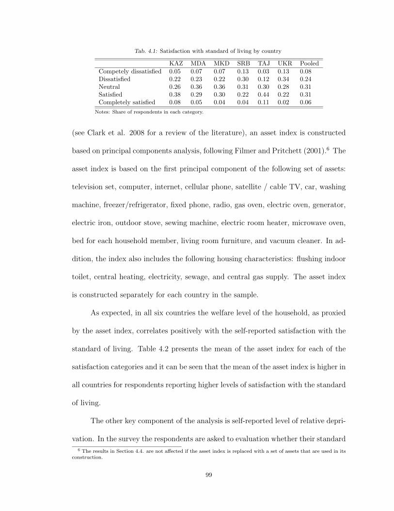
Tab. 4.1: Satisfaction with standard of living by country

KAZ MDA MKD SRB TAJ UKR PooledCompetely dissatisfied 0.05 0.07 0.07 0.13 0.03 0.13 0.08Dissatisfied 0.22 0.23 0.22 0.30 0.12 0.34 0.24Neutral 0.26 0.36 0.36 0.31 0.30 0.28 0.31Satisfied 0.38 0.29 0.30 0.22 0.44 0.22 0.31Completely satisfied 0.08 0.05 0.04 0.04 0.11 0.02 0.06

Notes: Share of respondents in each category.

(see Clark et al. 2008 for a review of the literature), an asset index is constructed

based on principal components analysis, following Filmer and Pritchett (2001).6 The

asset index is based on the first principal component of the following set of assets:

television set, computer, internet, cellular phone, satellite / cable TV, car, washing

machine, freezer/refrigerator, fixed phone, radio, gas oven, electric oven, generator,

electric iron, outdoor stove, sewing machine, electric room heater, microwave oven,

bed for each household member, living room furniture, and vacuum cleaner. In ad-

dition, the index also includes the following housing characteristics: flushing indoor

toilet, central heating, electricity, sewage, and central gas supply. The asset index

is constructed separately for each country in the sample.

As expected, in all six countries the welfare level of the household, as proxied

by the asset index, correlates positively with the self-reported satisfaction with the

standard of living. Table 4.2 presents the mean of the asset index for each of the

satisfaction categories and it can be seen that the mean of the asset index is higher in

all countries for respondents reporting higher levels of satisfaction with the standard

of living.

The other key component of the analysis is self-reported level of relative depri-

vation. In the survey the respondents are asked to evaluation whether their standard

6 The results in Section 4.4. are not affected if the asset index is replaced with a set of assets that are used in itsconstruction.

99

Tab. 4.2: Asset index by satisfaction level

KAZ MDA MKD SRB TAJ UKR PooledCompletely dissatisfied -1.75 -0.89 -2.33 -1.72 -0.86 -0.82 -1.37Dissatisfied -0.84 -0.71 -0.59 -0.41 -0.76 -0.35 -0.57Neutral -0.27 -0.29 0.03 0.39 -0.65 0.24 -0.10Satisfied 0.66 0.86 0.77 0.90 0.37 0.68 0.67Completely satisfied 1.13 1.40 1.24 1.03 1.42 0.71 1.24

Notes: Mean asset index in each category. The asset index is centered around zero;

negative values indicate lower welfare levels, positive values – higher welfare levels.

of living is better, same or worse than that of the majority of other people in (i) their

settlement (town or village); (ii) district of residence; (iii) country of residence. In

addition, the respondents are asked to state whether their parents and, separately,

grandparents had a higher/same/lower position in society when they were the same

age as the respondent.

Several observations can be made based on the distribution of responses to the

relative deprivation questions. Across countries the patterns of perceived relative

deprivation at local / regional and country levels appear to be broadly similar. Re-

spondents in Serbia report the highest levels of relative deprivation at all three levels

of geographic aggregation. This negativity echoes the greater levels of dissatisfac-

tion with the standard of living reported in Serbia (see Table 4.1). Furthermore,

the share of respondents who report a standard of living that is worse than that

of the majority of people in the village/town of residence is smaller than a similar

category at the district level, which in turn is lower than the country-level share

of those reporting to be relatively deprived. To understand why this should be the

case, note that since most of the respondents in a given country reside outside of the

capital city, the prevalence of those residing in relatively poor towns or villages who

are relatively deprived at the country level but not at the local level will be higher

100

than the prevalence of those residing in the capital, for instance, who are worse off

than their neighbours, but still better off than most the country’s citizens.

Tab. 4.3: Relative deprivation for various reference groups

KAZ MDA MKD SRB TAJ UKR PooledStandard of living relative to townWorse 0.174 0.222 0.169 0.245 0.142 0.197 0.191Same 0.649 0.573 0.598 0.554 0.599 0.655 0.605Better 0.151 0.157 0.190 0.164 0.203 0.0970 0.160N/A 0.00630 0.00407 0.00704 0.0146 0.0230 0.00815 0.0104Don’t know 0.0189 0.0448 0.0363 0.0229 0.0333 0.0426 0.0333Standard of living relative to districtWorse 0.234 0.305 0.206 0.358 0.301 0.239 0.272Same 0.564 0.467 0.587 0.483 0.442 0.563 0.518Better 0.152 0.116 0.146 0.0912 0.177 0.0807 0.128N/A 0.0141 0.00667 0.00852 0.0308 0.0248 0.0174 0.0168Don’t know 0.0352 0.106 0.0522 0.0371 0.0548 0.100 0.0648Standard of living relative to countryWorse 0.375 0.396 0.311 0.468 0.415 0.308 0.377Same 0.409 0.382 0.466 0.367 0.344 0.501 0.412Better 0.139 0.104 0.138 0.0820 0.132 0.0596 0.110N/A 0.0174 0.00741 0.0156 0.0333 0.0267 0.0174 0.0194Don’t know 0.0600 0.111 0.0696 0.0500 0.0826 0.114 0.0818Standard of living relative to parentsWorse 0.326 0.272 0.287 0.393 0.498 0.281 0.342Same 0.396 0.317 0.233 0.283 0.342 0.345 0.320Better 0.203 0.336 0.400 0.253 0.0900 0.310 0.266N/A 0.0237 0.00778 0.0126 0.0292 0.0185 0.0100 0.0167Don’t know 0.0515 0.0667 0.0674 0.0421 0.0511 0.0537 0.0557Standard of living relative to grandparentsWorse 0.196 0.204 0.126 0.224 0.287 0.161 0.199Same 0.264 0.186 0.120 0.205 0.264 0.188 0.204Better 0.343 0.401 0.528 0.353 0.204 0.453 0.381N/A 0.0396 0.0107 0.00926 0.0358 0.0315 0.0152 0.0235Don’t know 0.159 0.199 0.216 0.182 0.213 0.183 0.192Note: Share of respondents in each category, by country.

One of the questions explored in the next section pertains to the relative

salience of these various reference groups. Some insight into this question can be

gained by looking at the share of respondents who could not evaluate their relative

status at different levels of geographic proximity. This share increases in all countries

as the group relative to which one’s living standard is to be evaluated becomes less

local. It is perhaps not surprising that respondents find it easier to evaluate their

standard of living relative to a local – and thus more easily observable – reference

group. As the level of observability decreases, it becomes more difficult to evaluate

one’s relative deprivation. This can be argued to be prima facie evidence in favour

101

of local reference groups, since relative status can only be a salient concern if it

is observable. As the difficulty of relative comparisons increases, their importance

should generally decrease. I return to this issue in the next section.

In the case of relative deprivation vis-a-vis parents or grandparents, the dif-

ficulty of making a comparison is much higher in the case of grandparents. The

evaluations also tend to be more positive relative to grandparents than relative to

parents. They are also considerably more positive than local level comparisons -

whereas 16 percent of respondents in the overall sample viewed their standard of

living as better than that of the majority of other people in their village or town,

more than a quarter of respondents believe that their standard of living is higher

than the one enjoyed by their parents at similar age, and 38 percent believe that it

is higher than that of grandparents (more than half in FYROM).

Tab. 4.4: Relative status and household welfare (asset index)

KAZ MDA MKD SRB TAJ UKR PooledStandard of living relative to townWorse -1.06 -1.60 -1.53 -1.45 -1.12 -1.22 -1.35Same 0.01 0.25 0.18 0.41 -0.19 0.22 0.14Better 1.08 1.15 0.85 0.96 1.44 1.02 1.10Standard of living relative to districtWorse -0.98 -1.47 -1.37 -1.02 -0.92 -1.15 -1.15Same 0.14 0.56 0.25 0.65 0.09 0.31 0.32Better 1.06 1.52 0.92 0.93 1.44 1.18 1.19Standard of living relative to countryWorse -1.14 -1.08 -0.84 -0.64 -0.68 -0.88 -0.87Same 0.90 0.70 0.30 0.72 0.51 0.40 0.57Better 0.57 1.42 0.84 0.87 0.95 1.02 0.92Standard of living relative to parentsWorse -0.47 0.26 -0.07 -0.12 -0.05 -0.06 -0.09Same -0.05 -0.27 -0.09 0.11 -0.07 0.15 -0.04Better 0.63 -0.00 0.23 0.31 0.67 -0.06 0.21Standard of living relative to grandparentsWorse -0.52 -0.10 -0.17 -0.21 -0.07 -0.16 -0.20Same -0.30 -0.57 -0.22 0.09 -0.34 -0.14 -0.26Better 0.44 0.12 0.20 0.36 0.45 0.19 0.27

Notes: Mean asset index in each category.

102

Table 4.4 reports the mean of the asset index for each of the categories of

relative deprivation for each of the reference groups available in the data. Encour-

agingly, the value of the asset index is generally lowest for those who report to be

worse off vis-a-vis other groups, and highest for those who report to be better off.

The gradient is steepest for local reference groups, but less pronounced in the case

of comparisons vis-a-vis parents or grandparents.

Summary statistics for the variables used in the empirical analysis in the next

section are reported in Table 4.5. There are several notable differences between the

countries in the sample. For instance, in Tajikistan the share of heads of households

among respondents is considerably lower than in the rest of the countries, consistent

with the large-scale economic migration from Tajikistan to other countries in the

region, primarily Russia. Tajikistan is also the youngest country in the sample,

and has the highest share of population with primary education or less, which is

consistent with the fact that it is also the poorest country. The share of respondents

who are unemployed also varies considerably, from less than 10 percent in Moldova

and Ukraine to More than 20 percent in Tajikistan and Macedonia. In Ukraine

and in Macedonia the share of population residing in villages is roughly half the

level reported in Moldova and in Tajikistan. The share of population residing in

the country’s capital ranges from under 5 percent in Kazakhstan to more than 20

percent in Macedonia.

Tab. 4.5: Summary statistics by country

KAZ MDA MKD SRB TAJ UKR Pooled

Satisfaction 3.230 3.034 3.030 2.749 3.471 2.667 3.035(1.038) (0.996) (0.977) (1.059) (0.946) (1.033) (1.044)

Age 42.43 43.24 43.04 43.51 36.35 45.03 42.24(17.16) (18.05) (16.71) (16.41) (15.73) (18.58) (17.37)

Male 0.489 0.424 0.474 0.503 0.431 0.443 0.460

103

(0.500) (0.494) (0.499) (0.500) (0.495) (0.497) (0.498)Head of HH 0.524 0.491 0.409 0.495 0.286 0.541 0.457

(0.499) (0.500) (0.492) (0.500) (0.452) (0.498) (0.498)EducationPrimary or less 0.203 0.306 0.206 0.234 0.351 0.120 0.237

(0.402) (0.461) (0.404) (0.424) (0.477) (0.325) (0.425)Secondary 0.311 0.379 0.529 0.576 0.404 0.276 0.410

(0.463) (0.485) (0.499) (0.494) (0.491) (0.447) (0.492)Post-secondary 0.486 0.315 0.265 0.190 0.245 0.604 0.354

(0.500) (0.464) (0.441) (0.392) (0.430) (0.489) (0.478)Married 0.550 0.578 0.631 0.570 0.665 0.557 0.592

(0.498) (0.494) (0.483) (0.495) (0.472) (0.497) (0.491)Labour force statusPrivate sector 0.247 0.134 0.246 0.267 0.0734 0.208 0.195

(0.432) (0.341) (0.431) (0.443) (0.261) (0.406) (0.396)Public sector 0.171 0.194 0.136 0.160 0.126 0.197 0.164

(0.377) (0.395) (0.343) (0.367) (0.332) (0.398) (0.370)Self-employed 0.0591 0.0586 0.0426 0.0677 0.0999 0.0332 0.0600

(0.236) (0.235) (0.202) (0.251) (0.300) (0.179) (0.238)Unemployed 0.114 0.0976 0.289 0.188 0.234 0.0786 0.166

(0.318) (0.297) (0.454) (0.390) (0.423) (0.269) (0.372)Retired 0.189 0.213 0.160 0.188 0.0999 0.293 0.191

(0.392) (0.409) (0.367) (0.390) (0.300) (0.455) (0.393)Other 0.219 0.303 0.126 0.130 0.367 0.190 0.224

(0.414) (0.460) (0.332) (0.336) (0.482) (0.393) (0.417)Ln(HH size) 1.072 0.905 1.184 1.027 1.625 0.956 1.130

(0.586) (0.514) (0.461) (0.518) (0.473) (0.490) (0.563)Asset index 0.00408 -0.00237 0.00999 0.0255 0.00398 0.00885 0.00801

(2.430) (2.458) (2.027) (2.246) (2.349) (2.179) (2.287)Rural area 0.520 0.600 0.304 0.474 0.693 0.309 0.484

(0.500) (0.490) (0.460) (0.499) (0.461) (0.462) (0.500)NeighbourhoodElite 0.0138 0.00593 0.0295 0.00961 0.00745 0.00298 0.0116

(0.117) (0.0768) (0.169) (0.0976) (0.0860) (0.0545) (0.107)Higher middle class 0.131 0.297 0.340 0.213 0.367 0.123 0.246

(0.337) (0.457) (0.474) (0.410) (0.482) (0.328) (0.431)Lower middle class 0.669 0.612 0.546 0.686 0.484 0.661 0.608

(0.471) (0.487) (0.498) (0.464) (0.500) (0.473) (0.488)Poor 0.172 0.0812 0.0747 0.0869 0.116 0.205 0.123

(0.378) (0.273) (0.263) (0.282) (0.320) (0.404) (0.329)Slum 0.0149 0.00371 0.00896 0.00460 0.0257 0.00820 0.0111

(0.121) (0.0608) (0.0942) (0.0677) (0.158) (0.0902) (0.105)PropertyElite 0.00372 0.0182 0.0284 0.0242 0.0119 0.00745 0.0155

(0.0609) (0.134) (0.166) (0.154) (0.109) (0.0860) (0.123)Higher middle class 0.127 0.296 0.333 0.232 0.285 0.143 0.236

(0.333) (0.457) (0.471) (0.422) (0.451) (0.350) (0.425)Lower middle class 0.563 0.497 0.506 0.564 0.434 0.594 0.525

(0.496) (0.500) (0.500) (0.496) (0.496) (0.491) (0.499)Poor 0.222 0.143 0.105 0.132 0.168 0.218 0.165

(0.415) (0.350) (0.306) (0.338) (0.374) (0.413) (0.371)Slum 0.0305 0.0263 0.0175 0.0418 0.0667 0.0332 0.0359

(0.172) (0.160) (0.131) (0.200) (0.250) (0.179) (0.186)N/A 0.0543 0.0197 0.0105 0.00669 0.0350 0.00559 0.0222

(0.227) (0.139) (0.102) (0.0815) (0.184) (0.0746) (0.147)

Note: Mean of each variable with standard deviation in parentheses.

104

4.4 Empirical analysis

4.4.1 Salience of different reference groups

In investigating the relative salience of different reference groups I follow the

empirical setup in Senik (2009). Table 4.6 presents estimates of regressions which

include the three geographic relative deprivation metrics (at local, district, and

country levels) as well as the relative deprivation vis-a-vis the standard of living

held by the parents. The comparison with grandparents is not considered due to

the high share of respondents who were not able to rank their own standard of living

vis-a-vis the one enjoyed by their grandparents, suggesting that it is not the most

natural reference group. As in Senik (2009) OLS regressions are estimated for ease of

interpretation.7 The baseline category is composed by those who reported the same

standard of living vis-a-vis all four reference categories (locality, district, country,

and parents). Results for the pooled regression are in column (1) and columns (2)-(7)

present separate regression for each of the countries in the sample. All regressions

account account for the respondent’s age, age squared, sex, education level, marital

status, employment status, as well as household size, area of residence, the asset

index and whether the respondent is the head of household. All regressions also

include a set of district dummies.

Several observations can be made about the estimated coefficients. For all

three geographic measures of relative deprivation considering your own standard of

7 Ferrer-i-Carbonell and Frijters (2005) examine the more stringent assumption of cardinality, i.e. that thedifference between responses 2 and 3 on the satisfaction scale is the same, for instance, as the difference between 6and 7. Relying on data from the German Socio-Economic Panel (GSOEP) they look at differences between ordinaland cardinal models of life satisfaction using the 11-step response to the following question: “How happy are youat present with your life as a whole? Please answer by using the following scale in which 0 means totally unhappy,and 10 means totally happy.” They find that results are largely unaffected by the choice of cardinal vs. ordinalspecification.

105

living as being worse that the majority of people in that group is negatively associ-

ated with reported satisfaction with the standard of well-being, and the opposite it

true for those who assess their standard of living as being “better”. In the case of

relative deprivation vis-a-vis parents, a negative assessment similarly has a negative

association with reported satisfaction, whereas having a higher standard of living

vis-a-vis parents does not appear to boost reported satisfaction, a results consistent

with adaptive preferences (Frederick and Loewenstein 1999; Easterlin 2001; Stutzer

2004; Di Tella et al. 2010), and in particular with more prominent adaptation over

the domain of gains (Arkes et al, 2006).

Table 4.6 also presents two sets of tests. First, across all reference groups

there is an apparent asymmetry in the sense that the magnitude of the estimates

associated with a negative assessment is larger than that for the positive assessment.

This was also observed by Senik (2009). I perform formal tests which compare the

magnitude of the negative coefficient associated with the “worse” relative status

assessment in a given group and the positive coefficient associated with the “better”

relative status (e.g. in the town case, I test the hypothesis H0 : β1t + β3t = 0).

In the case of relative deprivation vis-a-vis parents the magnitude of the negative

assessments is larger than that of the positive assessments. For geographic reference

groups this is also the case in the pooled sample, albeit in the individual country

regressions the null hypothesis cannot be rejected in 14 out out 18 tests.8

Secondly, I test the relative salience of different reference groups by comparing

the magnitudes of the coefficients associated with perceived relative deprivation

8 The larger magnitudes associated with negative assessments is in the spirit of loss aversion (Kahneman andTversky, 1979), although the evidence is merely suggestive, since income differences associated with “worse” and“better” need not be the same. I am grateful to Andrew Clark for pointing this out.

106

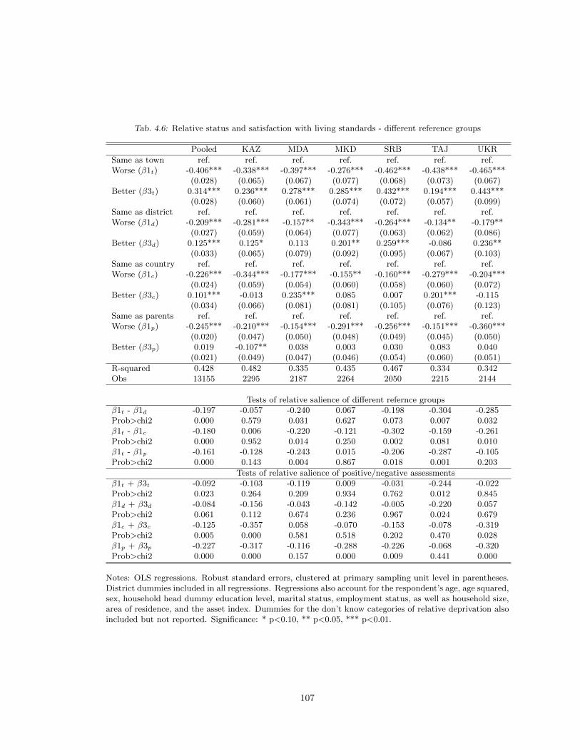
Tab. 4.6: Relative status and satisfaction with living standards - different reference groups

Pooled KAZ MDA MKD SRB TAJ UKR

Same as town ref. ref. ref. ref. ref. ref. ref.Worse (β1t) -0.406*** -0.338*** -0.397*** -0.276*** -0.462*** -0.438*** -0.465***

(0.028) (0.065) (0.067) (0.077) (0.068) (0.073) (0.067)Better (β3t) 0.314*** 0.236*** 0.278*** 0.285*** 0.432*** 0.194*** 0.443***

(0.028) (0.060) (0.061) (0.074) (0.072) (0.057) (0.099)Same as district ref. ref. ref. ref. ref. ref. ref.Worse (β1d) -0.209*** -0.281*** -0.157** -0.343*** -0.264*** -0.134** -0.179**

(0.027) (0.059) (0.064) (0.077) (0.063) (0.062) (0.086)Better (β3d) 0.125*** 0.125* 0.113 0.201** 0.259*** -0.086 0.236**

(0.033) (0.065) (0.079) (0.092) (0.095) (0.067) (0.103)Same as country ref. ref. ref. ref. ref. ref. ref.Worse (β1c) -0.226*** -0.344*** -0.177*** -0.155** -0.160*** -0.279*** -0.204***

(0.024) (0.059) (0.054) (0.060) (0.058) (0.060) (0.072)Better (β3c) 0.101*** -0.013 0.235*** 0.085 0.007 0.201*** -0.115

(0.034) (0.066) (0.081) (0.081) (0.105) (0.076) (0.123)Same as parents ref. ref. ref. ref. ref. ref. ref.Worse (β1p) -0.245*** -0.210*** -0.154*** -0.291*** -0.256*** -0.151*** -0.360***

(0.020) (0.047) (0.050) (0.048) (0.049) (0.045) (0.050)Better (β3p) 0.019 -0.107** 0.038 0.003 0.030 0.083 0.040

(0.021) (0.049) (0.047) (0.046) (0.054) (0.060) (0.051)

R-squared 0.428 0.482 0.335 0.435 0.467 0.334 0.342Obs 13155 2295 2187 2264 2050 2215 2144

Tests of relative salience of different refernce groupsβ1t - β1d -0.197 -0.057 -0.240 0.067 -0.198 -0.304 -0.285Prob>chi2 0.000 0.579 0.031 0.627 0.073 0.007 0.032β1t - β1c -0.180 0.006 -0.220 -0.121 -0.302 -0.159 -0.261Prob>chi2 0.000 0.952 0.014 0.250 0.002 0.081 0.010β1t - β1p -0.161 -0.128 -0.243 0.015 -0.206 -0.287 -0.105Prob>chi2 0.000 0.143 0.004 0.867 0.018 0.001 0.203

Tests of relative salience of positive/negative assessmentsβ1t + β3t -0.092 -0.103 -0.119 0.009 -0.031 -0.244 -0.022Prob>chi2 0.023 0.264 0.209 0.934 0.762 0.012 0.845β1d + β3d -0.084 -0.156 -0.043 -0.142 -0.005 -0.220 0.057Prob>chi2 0.061 0.112 0.674 0.236 0.967 0.024 0.679β1c + β3c -0.125 -0.357 0.058 -0.070 -0.153 -0.078 -0.319Prob>chi2 0.005 0.000 0.581 0.518 0.202 0.470 0.028β1p + β3p -0.227 -0.317 -0.116 -0.288 -0.226 -0.068 -0.320Prob>chi2 0.000 0.000 0.157 0.000 0.009 0.441 0.000

Notes: OLS regressions. Robust standard errors, clustered at primary sampling unit level in parentheses.District dummies included in all regressions. Regressions also account for the respondent’s age, age squared,sex, household head dummy education level, marital status, employment status, as well as household size,area of residence, and the asset index. Dummies for the don’t know categories of relative deprivation alsoincluded but not reported. Significance: * p<0.10, ** p<0.05, *** p<0.01.

107

across reference groups (e.g. H0 : β1t − β1d = 0 tests the relative salience of town-

based vs district-based relative status comparisons). In five out of seven cases the

negative coefficient associated with relative deprivation at the local (village / town)

level is larger in magnitude than the coefficient associated with relative deprivation

at the district level. Similarly in 5 out of 7 tests it is also larger than the coefficient

associated with relative deprivation at the country level. This provides some support

for the salience of localised relative deprivation in particular, and is consistent with

the earlier results which suggested that relative deprivation at the local level was

easiest for respondents to evaluate.

As Senik (2009) notes, one of the difficulties with the above results has to do

endogeneity resulting from with the fact that perceptions of relative deprivation and

satisfaction with standard of living can both be a function of unobserved traits. To

account for this possibility, Senik proposes to look at respondents who are better off

on one dimension, but worse off on another. The identifying assumption is that while

those with universally positive (negative) assessments of their relative standard of

living may be generally more optimistic (pessimistic) for reasons we do not observe,

there is “[n]o obvious omitted variable or reverse causation is available for these

concomitant opposite variations.”

Following Senik (2009) I evaluate the salience of different reference groups by

looking at the interactions of relative deprivation assessments for different groups

that go in opposite directions. Thus, for relative deprivation at town level and rel-

ative deprivation at district level this interaction generates nine categories, two of

which are of interest: (i) worse at town level and better at district level; and (ii)

108

Tab. 4.7: Relative status and satisfaction with living standards - interactions

(1) (2) (3) (4) (5) (6)

Below town, above district -0.294**(0.128)

Above town, below district -0.114(0.078)

Below town, above country -0.143(0.106)

Above town, below country -0.001(0.052)

Below district, above country -0.060(0.101)

Above district, below country -0.131*(0.070)

Below town, above parents -0.741***(0.040)

Above town, below parents 0.183***(0.043)

Below district, above parents -0.624***(0.034)

Above district, below parents 0.112**(0.045)

Below country, above parents -0.544***(0.034)

Above country, below parents 0.042(0.050)

R-squared 0.411 0.413 0.394 0.409 0.398 0.387Obs 13155 13155 13155 13155 13155 13155

Notes: OLS regressions. Two interactions reported, but all interactions included in the regressions. Robuststandard errors, clustered at primary sampling unit level in parentheses. District dummies included in allregressions. Regressions also account for the respondent’s age, age squared, sex, household head dummyeducation level, marital status, employment status, as well as household size, area of residence, and theasset index. Dummies for the don’t know categories of relative deprivation also included but not reported.Significance: * p<0.10, ** p<0.05, *** p<0.01.

better at town level and worse at district level. Similar groups are constructed for

town×country, town×parents, district×country, district×parents, and country×parents

pairs.

The estimates of regressions with reference group interactions are presented in

Table 4.7. Only estimates of the worse/better interactions are reported, although

all nine cross-categories are included in all regressions. The regressions also account

for the full set of controls. Columns (1)-(3) look at local interactions of relative

deprivation at town, district and country level, whereas columns (4)-(6) report the

interaction of relative deprivation vis-a-vis parents with each of geographic reference

109

groups. From (1)-(3) it is not possible to infer any notable ranking of the importance

of different geographic reference groups. On the other hand, estimates of models

(4)-(6) suggest that relative deprivation defined in terms of geographic space is more

salient than deprivation vis-a-vis parents. The sign of the coefficient in all of the

cases is based on whether one reports to be worse or better than others in their

locality/district/country of residence. Relative deprivation in this geographic sense

is not fully compensated by an improved standard of living relative to the one enjoyed

by parents. Having a standard of living higher than the majority of people in the

town or district of residence still has a positive effect on overall satisfaction with the

standard of living, even if this standard of living is perceived by the respondent to

be below the level enjoyed by her parents. The patterns are again in line with loss

aversion, estimates being larger in magnitude over the domain of losses. Finally,

deprivation at the village/town level appears to be the most salient geographic

reference group in terms of the magnitudes of impact.

4.4.2 More on local relative deprivation - IV results

The results in section 4.4.1 suggested that relative deprivation defined in terms

of geographic space is more salient for overall satisfaction with the standard of living

compared with relative deprivation vis-a-vis one’s parents. Furthermore, the results

are consistent with previous evidence that reference groups are likely to be very

local (Graham and Felton 2006; Knight et al. 2009; Kuhn et al. 2011). In this

section I look more closely at local relative deprivation. In particular, I employ an

instrumental variables approach to estimate a causal effect of relative deprivation

on satisfaction with the standard of living.

110

I start by assuming that satisfaction with one’s living standard is a function of

the living standard itself (in an absolute sense), relative status considerations, and

relevant characteristics of the respondent/household/area of residence, expressed as

follows:

Si = β1LSi + β2RDPi +X

′iγ + εi,

where Si is satisfaction with living standard, LSi is objective living standard, mea-

sured by means of an asset index, RDPi is relative deprivation at the town level

as perceived by individual i, Xi is a set of personal and household characteristics

that determine one’s satisfaction as before. For the moment it is assumed that

Cov(RDPi , εi) = 0. The relationship between satisfaction and local relative depri-

vation thus defined is reported in Table 4.8. As before, lower relative status is

negatively associated with one’s satisfaction with the standard of living both in the

pooled sample and in each of the individual countries in the survey. 9

It is possible, however, that the error term εi includes unobserved cognitive

traits Cogi that are correlated both with RDPi and with Si, such that εi = θCogi+ui,

and Cov(RDPi , εi) 6= 0, while Cov(RDP

i , ui) = 0.10 For instance, respondents who

are better off than their neighbours may report instead that their standard of living

is the same as that of their neighbours out of modesty or unwillingness to admit

their superior relative standing. Modest individuals may, at the same time, be more

content with their own standard of living due to the same unobservables.

9 Here relative deprivation is used as an index where higher values indicate better relative standing, in spite ofthe fact that this is an ordinal variable with no natural scale. For this reason of primary interest is the sign of thecoefficient, and not its magnitude. Note, however, that the estimates in table 4.6 suggested that the effect of movingfrom “worse” to “same” and from “same” to “better” is of equal magnitude. The results are substantively the samewhen relative deprivation is defined instead as a dummy variable that equals 1 if the respondent stated that herstandard of living is worse than that of the majority of people in her village/town of residence, and zero otherwise.10 Identification requires that Cogi not be systematically correlated with LSi and Xi, including (perhaps strongly)

age, sex and education level.

111

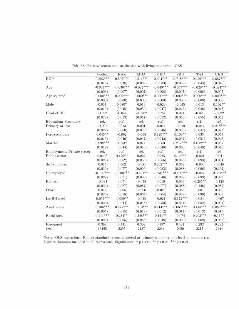
Tab. 4.8: Relative status and satisfaction with living standards - OLS


RDP 0.583*** 0.507*** 0.514*** 0.604*** 0.718*** 0.429*** 0.667***(0.016) (0.038) (0.039) (0.033) (0.038) (0.043) (0.048)

Age -0.034*** -0.036*** -0.024*** -0.046*** -0.047*** -0.029*** -0.024***(0.003) (0.007) (0.007) (0.008) (0.007) (0.008) (0.007)

Age squared 0.000*** 0.000*** 0.000*** 0.000*** 0.000*** 0.000*** 0.000***(0.000) (0.000) (0.000) (0.000) (0.000) (0.000) (0.000)

Male 0.031 0.080* 0.019 -0.029 -0.045 0.013 0.102**(0.019) (0.045) (0.050) (0.047) (0.045) (0.046) (0.048)

Head of HH -0.022 -0.044 -0.098* 0.024 0.061 -0.025 -0.022(0.022) (0.053) (0.057) (0.052) (0.050) (0.055) (0.053)

Education: Secondary ref. ref. ref. ref. ref. ref. ref.Primary or less -0.001 0.013 0.001 -0.074 -0.019 -0.044 0.218***

(0.022) (0.060) (0.048) (0.046) (0.055) (0.047) (0.073)Post-secondary 0.045** -0.002 -0.064 0.120*** 0.109** 0.035 0.053

(0.019) (0.046) (0.047) (0.042) (0.052) (0.051) (0.046)Married 0.098*** 0.073* 0.074 0.050 0.217*** 0.158*** 0.067

(0.019) (0.044) (0.050) (0.046) (0.050) (0.049) (0.046)Employment: Private sector ref. ref. ref. ref. ref. ref. ref.Public sector 0.045* 0.126** 0.022 0.025 0.140** -0.021 -0.041

(0.026) (0.062) (0.063) (0.056) (0.063) (0.093) (0.061)Self-employed 0.015 0.002 -0.081 0.262*** 0.058 -0.060 -0.048

(0.036) (0.077) (0.095) (0.083) (0.088) (0.096) (0.132)Unemployed -0.192*** -0.200*** -0.191** -0.234*** -0.166*** -0.027 -0.331***

(0.027) (0.071) (0.080) (0.046) (0.059) (0.093) (0.083)Retired -0.034 0.071 -0.038 0.010 0.099 -0.285** -0.128

(0.036) (0.087) (0.087) (0.077) (0.088) (0.126) (0.085)Other 0.012 0.005 -0.006 -0.025 0.086 0.001 0.060

(0.026) (0.058) (0.064) (0.064) (0.069) (0.090) (0.066)Ln(HH size) -0.057*** -0.089** -0.035 -0.021 -0.172*** 0.084 -0.067

(0.020) (0.044) (0.048) (0.050) (0.044) (0.052) (0.054)Asset index 0.106*** 0.177*** 0.119*** 0.114*** 0.065*** 0.118*** 0.083***

(0.005) (0.015) (0.013) (0.012) (0.011) (0.013) (0.015)Rural area 0.111*** 0.234** 0.248*** 0.111** -0.074 0.203*** 0.115*

(0.026) (0.095) (0.068) (0.048) (0.050) (0.069) (0.066)

R-squared 0.393 0.441 0.303 0.397 0.431 0.292 0.294Obs 13155 2295 2187 2264 2050 2215 2144

Notes: OLS regressions. Robust standard errors, clustered at primary sampling unit level in parentheses.District dummies included in all regressions. Significance: * p<0.10, ** p<0.05, *** p<0.01.

112

Furthermore, a large share of respondents report that their standard of living

is the same as that of the majority of residents in their town (and similarly for

district) of residence. Roh (2011) shows that the tendency of choosing the middle

category, oftentimes observed in responses to attitudinal questions, will introduce

non-classical measurement error into independent variables (here RDPi ) that will

generally bias downward the regression coefficient on those variables.

In order to extract exogenous variation in the relative deprivation variable, I

rely on the interviewer’s own assessment of the respondent’s relative deprivation.

Specifically, the interviewer provides an evaluation of the conditions inside the re-

spondent’s property, coded as one of the following: elite, higher middle class, lower

middle class, poor, or slum. The interviewer is also asked to provide an assessment

of the conditions of the neighbourhood where the respondent’s household is located,

similarly ranging from elite to slum. Based on this I create an index defined as the

difference between the neighbourhood score and the household score, where positive

values indicate that the household conditions are better than those of the neigh-

bourhood, and negative values indicate that the household’s conditions are worse

than those of the neighbourhood where it is located. 11 The index ranges from -2

to +2.12

Perceptions of relative deprivation RDPi are assumed to be determined as

follows:

RDPi = δRDa

i +X′iζ + υi, where RDa

i is actual relative deprivation, Xi is the

same set of controls as before, and Cogi is not observed and is part of a composite

11 Note that results do not change if instead RDIi is defined as a dummy variable which evaluates to 1 if the

conditions of the neighbourhood are better than the conditions of the property, and zero otherwise.12 There are only few observations with an index of -3 (a total of 33 in the pooled sample, most from Tajikistan)

or +3 (a total of 6 in the pooled sample), these are recoded as -2 and +2 respectively.

113

error term υi = ϕCogi + ϑi.

Note that RDai is not observed. Instead, we observe the interviewer’s as-

sessment of relative deprivation RDIi , which serves as a proxy for actual relative

status, i.e. RDIi = ρRDa

i + ωi, where ωi is assumed uncorrelated with RDai .

Thus, RDPi = ψRDI

i + X′iζ + ηi, where ψ = δ

ρand ηi = υi − δ

ρωi. It is as-

sumed that Cov(RDai , υi) = 0, i.e. objective relative deprivation is not correlated

with unobservable cognitive biases in the error term. It is similarly assumed that

Cov(RDIi , υi) = 0, i.e. any possible cognitive biases of the interviewer are not sys-

tematically linked with those of the respondent. It is plausible that RDai and RDI

i

are reasonably well correlated.

In order for RDIi to serve as an instrument for relative deprivation the first

requirement is that it has to be the case that ψ 6= 0, i.e. RDIi has to be partially

correlated with RDPi conditional on all of the other exogenous variables (here LSi

and the vector Xi). This assumption is testable. Table 4.10 reports the tests of weak

identification based on the Kleibergen-Paap Wald F statistic (Kleibergen and Paap

2006). In all cases the F statistic exceeds the critical values for weak identification

proposed in Stock and Yogo (2005). RDIi is strongly predictive of perceived relative

deprivation both in the pooled sample and in the individual country sub-samples.

The second requirement is Cov(RDIi , εi) = 0. For this to hold it has to be

the case that RDIi only affects satisfaction with one’s living standard through per-

ceptions of relative deprivation, which in turn affect Si. As argued above, it seems

plausible that the interviewer’s RDIi is not correlated with the respondent’s unob-

served Cogi.13 It is plausible that perceived relative status affects satisfaction with

13 One may worry that the interviewer’s assessment of the respondent’s relative deprivation may be influenced by

114

Tab. 4.9: Relative status and satisfaction with living standards - 2SLS


RDP 1.371*** 2.348*** 0.782*** 1.432*** 1.358*** 1.518*** 1.296***(0.143) (0.627) (0.279) (0.404) (0.320) (0.377) (0.410)

Obs 12873 2174 2145 2237 2035 2146 2136Endogeneity test 35.633 20.778 0.896 4.856 4.685 11.691 2.664P-value 0.000 0.000 0.344 0.028 0.030 0.001 0.103Kleibergen-Paap statistic 145.055 12.927 38.872 14.815 30.212 25.889 19.332

Notes: 2SLS regressions. Robust standard errors, clustered at primary sampling unit level in parentheses.Full set of controls. Interviewer’s assessment of the entrance of the property and of the property itself usedas instruments. Significance: * p<0.10, ** p<0.05, *** p<0.01.

living standard. For Cov(RDIi , εi) = 0 to hold it also has to be the case that the

respondent’s relative deprivation per se, when the respondent is not aware that she

is relatively deprived, does not have an effect on her standard of living satisfac-

tion. It can be argued that relative deprivation can be negatively associated with

satisfaction, even when unobserved, because it is a by-product of a low standard

of living, which is negatively associated with satisfaction. The IV set-up thus im-

plicitly requires that the observed LSi capture one’s objective absolute standard of

living in some complete sense, such that there is no unobserved living standard in

εi. Finally, since RDIi is constructed as the difference between the property and the

neighbourhood living standard assessments, the possibility of the middle response

style affecting the interviewer as well will not be problematic as long as the response

style is stable across the two questions, and it is difficult to think of reasons why

this should not be the case.

The estimates for 2SLS regressions in which interviewer’s assessments are used

to instrument relative deprivation are reported in Table 4.10. In addition to the

the mood of the respondent. There are two factors mitigating this possibility. First, the interviewer is not asked toprovide a direct assessment of relative deprivation, rather the assessment of the neighbourhood and the assessmentof the property are provided separately, and these two questions are not consecutive. Secondly, in the questionnairethe respondent’s assessment of relative status is in the first half of the interview, whereas the respondent’s assessmentis provided at the end of the interview, after attitudinal questions that do not probe the respondent’s welfare ineither absolute or relative terms.

115

weak identification tests discussed above I also report the results of an endogeneity

test, defined as the difference between two Sargan-Hansen statistics: one for the

equation where the relative deprivation is treated as endogenous, and one for the

equation with the larger set of instruments, where it is treated as exogenous. With

the exception of Moldova and (marginally, Ukraine) the null hypothesis that the

relative deprivation measure is exogenous is rejected at conventional levels. Subject

to the validity of the IV approach, the 2SLS estimates confirm the negative effect of

local relative deprivation on satisfaction with one’s standard of living, both in the

pooled sample, and in the individual country samples.

Notably, 2SLS estimates are larger than OLS estimates, particularly in the case

of Kazakhstan, although here the estimate is very imprecise. The higher second stage

estimates are consistent with the downward OLS bias due to the measurement error

introduced by the middle response style. Reporting that one’s living standard is no

higher than of the majority of settlement residents due to unobserved traits such as

modesty would also bias the OLS results downward. Finally, note that the positive

(negative) effect on one’s satisfaction with the standard of living of reporting a higher

(lower) living standard vis-a-vis others in one’s settlement increases (decreases) with

the interviewer’s assessment (i.e. the positive satisfaction effect of reporting a better

living standard is greatest in magnitude when matched by an assessment of “better”

by the interviewer, and decreases in magnitude when the interviewer’s assessment

is “same”, or “lower”). Since the scale of worse/same/better is coarse, it is plausible

that households with a very high standard of living will be more likely to be ranked

as better than others by both the respondent and the interviewer, and similarly

116

household with a very low standard of living will be more likely to get a consistently

negative assessment. This would also suggest higher second stage estimates.


The existing evidence of the importance of relative deprivation for well-being is

generally (i) derived from data for OECD countries; (ii) based on relative deprivation

metrics that are imposed by the researcher, an assumption the validity of which is

difficult to test; and (iii) does not always fully address the potential endogeneity

biases, especially in cross-sectional studies.

This study aimed to address all three of the above shortcomings. It found

a negative effect of local relative deprivation on satisfaction with one’s standard

of living based on data from six Transition Economies, including Tajikistan and

Moldova - the poorest countries in post-Socialist Europe. The estimates of the

negative effect of relative deprivation were based on respondent-defined measures of

relative deprivation that do not suffer from status observability or status salience

concerns associated with researcher-imposed relative deprivation metrics. Finally,

an instrumental variables empirical strategy was adopted in order to establish a

causal effect of relative deprivation on well-being.

Several other findings emerge from this study. First, while the true reference

groups are multidimensional and ultimately unobserved, the data suggest that rela-

tive deprivation based on geographic reference groups is more salient than that based

on comparisons vis-a-vis parents, and within the category of geographic reference

groups, local reference groups are more salient than broader country-wide assess-

ments of relative status. Second, relative deprivation is a welfare-relevant concern

117

even at low income levels. This conclusion is in line with the recent findings by

Fafchamps and Shilpi (2008) from Nepal, but contradict the Ravallion and Lokshin

(2010) results from Malawi where relative deprivation mattered only for the well-off.

118

5 Overall conclusion

Amartya Sen’s question “Equality of What?”, posed in his 1979 Tanner Lec-

tures and concerned with the relevant space over which equality should be considered

for purposes of justice, is an important and highly contested subject in the distribu-

tive justice literature. A number of alternatives have been suggested, including

equality of resources (Rawls 1971; Dworkin 1981), equality of opportunities for wel-

fare (Arneson 1989), equality of opportunity for a good life (Arneson 2000), equality

of access to advantage (G. A. Cohen 1989), or equality of capabilities (Sen 1980,

2000), among others. Meanwhile, at international development institutions like the

World Bank, and in the current policy discourse that is increasingly concerned with

the growing economic inequality in many countries, the main concept of inequality

in use is that of income inequality. Until recently, the fields of distributive justice

and development economics did not communicate effectively on this important is-

sue. While the former identified inequalities that matter, these were difficult to

measure, and hence difficult to use effectively in development policies. The latter

provided us with precise magnitudes of inequality across space and time, but it is

not clear that what was being measured was the relevant inequality space, or even

the degree to which it approximated the relevant inequality space as described by

political philosophers.

However, the extent and the implications of inequality of opportunity – and its

relation to overall inequality – are becoming increasingly important in analytical and

policy debates. The provision of equal opportunities for all is moving to the forefront

119

of social policy not only in the European Union but also in other parts of the world.

In Latin America a number of countries track the evolution of the recently developed

Human Opportunity Index (HOI) and in several countries (Mexico, Chile) policies

aim directly at the improvement of the HOI.

To the extent that status concerns and inequality of opportunity trap develop-

ment in low level equilibria, as was eloquently articulated by the World Development

Report 2006 on Equity and Development, it is knowledge based on developing coun-

tries that is most vital for policy purposes. This dissertation aimed to contribute to

our knowledge base in this area by adding an account of the importance of inequal-

ity of opportunity in post-Socialist Europe for preferences over redistributive policy

and expectations of future social mobility. The concept of inequality of opportunity

examined derived in part from Rawls’s concept of fair equality of opportunity based

on access to positions and offices in society, and in part it is based on beliefs about

the importance of effort and luck for success. This is but one of many ways of

looking at this issue. A growing literature that builds on the work of John Roemer

examines inequality of opportunity by separating overall inequality into that due to

effort and that due to pre-determined circumstances. This literature is in its early

stage of development, and the findings of this dissertation support further analytical

efforts aimed at capturing the various dimensions of inequality of opportunity both

in developed and developing countries, understanding its drivers, and ways in which

it can be alleviated through policy interventions.

This dissertation drew on data from Transition Economies, which, due to the

rapid changes since 1989 over a very short period of time, provided an ideal setting

120

for investigating aspects of inequality aversion and relative deprivation. This is be-

cause the magnitude of the socio-economic transformation is large enough to upset

prior stable expectations of the citizens of this region, while the speed of the trans-

formation ensured that the effect of adaptive preferences is only partial. This raises a

question, however, vis-a-vis the relevance of the findings of this dissertation for other

developing countries such as those in Latin America, where high levels of inequality

existed for much longer periods of time. While long-term deprivation and inequality

may certainly give rise to adaptation, possibly weakening the link between inequal-

ity and life satisfaction, it should still be the case that expectations of one’s future

chances of mobility will suffer on account of inequality of opportunity. Furthermore,

as suggested by Alesina and Angeletos (2005), preferences over redistributive policy

will still be affected (and reinforced) by perceptions of persistent institutional un-

fairness, resulting in multiple equilibria. As the result, improvements of the formal

institutions aimed at leveling the playing field and enlarging the opportunity set

of all – and especially of those in the lower tail of the bottom to escape inequality

traps.

121

Bibliography

Alesina, A., Di Tella, R. and MacCulloch, R. (2004) Inequality and happiness: are

europeans and americans different?, Journal of Public Economics, 88, 2009–2042.

Alesina, A. F. and Angeletos, G.-M. (2005) Fairness and redistribution, The Amer-

ican Economic Review, 95, pp. 960–980.

Alesina, A. F. and Giuliano, P. (2009) Preferences for redistribution, NBER Working

Papers 14825, National Bureau of Economic Research, Inc.

Alesina, A. F. and La Ferrara, E. (2005) Preferences for redistribution in the land

of opportunities, Journal of Public Economics, 89, 897–931.

Appadurai, A. (2004) The capacity to aspire: culture and the terms of recognition,

in Culture and Public Action (Eds.) V. Rao and M. Walton, Stanford University

Press, pp. 59–84.

Arkes, H., Hirshleifer, D., Jiang, D. and Lim, S. (2006) Reference point adaptation:

Tests in the domain of security trading, Tech. rep., University Library of Munich,

Germany.

Arneson, R. J. (1989) Equality and equal opportunity for welfare, Philosophical

Studies, 56, 77 – 93.

Arneson, R. J. (2000) Economic analysis meets distributive justice, Social Theory

and Practice: An International and Interdisciplinary Journal of Social Philosophy,

26(2), 327–345.

Atkinson, A. B. (1970) On the measurement of inequality, Journal of Economic

Theory, 2, 244–263.

Beegle, K., De Weerdt, J., Friedman, J. and Gibson, J. (2010) Methods of household

consumption measurement through surveys : experimental results from tanzania,

Policy Research Working Paper Series 5501, The World Bank.

Beegle, K., Himelein, K. and Ravallion, M. (2009) Frame-Of-Reference bias in sub-

jective welfare regressions, Research Working papers, 1, 1–36.

Bellemare, C., Kroger, S. and Van Soest, A. (2008) Measuring inequity aversion in

a heterogeneous population using experimental decisions and subjective probabil-

ities, Econometrica, 76, 815–839.

Benabou, R. and Ok, E. A. (2001) Social mobility and the demand for redistribution:

The poum hypothesis, The Quarterly Journal of Economics, 116, 447–487.

Benabou, R. and Tirole, J. (2006) Belief in a just world and redistributive politics,

The Quarterly Journal of Economics, 121, 699–746.

Blanchflower, D. G. and Oswald, A. J. (2004) Well-being over time in britain and

the USA, Journal of Public Economics, 88, 1359–1386.

Bourguignon, F., Ferreira, F. H. G. and Menendez, M. (2003) Inequality of outcomes

and inequality of opportunities in brazil, Tech. rep., Department of Economics

PUC-Rio (Brazil).

Bourguignon, F., Ferreira, F. H. G. and Walton, M. (2006) Equity, efficiency and

inequality traps: A research agenda, The Journal of Economic Inequality, 5, 235–

256.

123

Bozeat, N., Irving, P., Ramos, X., Vincze, M., Juravle, C. and Jesuit, D. (2010)

Social mobility and intra-regional income distribution across eu member states,

Tech. rep., European Commission, DG Regional Policy.

Brown, P. H., Bulte, E. and Zhang, X. (2011) Positional spending and status seeking

in rural china, Journal of Development Economics, 96, 139–149.

Camerer, C. F. and Thaler, R. H. (1995) Ultimatums, dictators and manners, Jour-

nal of Economic Perspectives, IX, 209–219.

Checchi, D. and Filippin, A. (2004) An Experimental Study of the POUM Hypoth-

esis, Research on Economic Inequality, 11, 115–136.

Checchi, D. and Peragine, V. (2010) Inequality of opportunity in italy, Journal of

Economic Inequality, 8, 429–450.

Chen, X. and Zhang, X. (2009) Blood for social status: Preliminary evidence from

rural china, 2009 Annual Meeting, July 26-28, 2009, Milwaukee, Wisconsin 49411,

Agricultural and Applied Economics Association.

Clark, A. E. (2003) Unemployment as a social norm: Psychological evidence from

panel data, Journal of Labor Economics, 21, 289–322.

Clark, A. E., Frijters, P. and Shields, M. A. (2008) Relative income, happiness, and

utility: An explanation for the easterlin paradox and other puzzles, Journal of

Economic Literature, 46, 95–144.

Clark, A. E. and Oswald, A. J. (1996) Satisfaction and comparison income, Journal

of Public Economics, 61, 359–381.

124

Clark, A. E. and Senik, C. (2010) Who compares to whom? the anatomy of income

comparisons in europe*, The Economic Journal, 120, 573–594.

Clark, A. E. and Senik, C. (2011) Will gdp growth increase happiness in developing

countries?, IZA Discussion Papers 5595, Institute for the Study of Labor (IZA).

Cogneau, D. and Mesple-Somps, S. (2008) Inequality of opportunity for income in

five countries of africa, in Research on Economic Inequality, Emerald (MCB UP

), Bingley, vol. 16, pp. 99–128.

Cohen, G. A. (1989) On the currency of egalitarian justice, Ethics, 99, 906–944.

Corneo, G. and Gruner, H. P. (2002) Individual preferences for political redistribu-

tion, Journal of Public Economics, 83, 83–107.

D’Ambrosio, C. and Frick, J. R. (2007) Income satisfaction and relative deprivation:

An empirical link, Social Indicators Research, 81, pp. 497–519.

Deaton, A. (2001) Relative deprivation, inequality, and mortality, NBER Working

Paper 8099, National Bureau of Economic Research.

Deaton, A. (2007) Income, aging, health and wellbeing around the world: Evidence

from the gallup world poll, Tech. rep., National Bureau of Economic Research,

Inc.

Deaton, A. and Zaidi, S. (1999) Guidelines for constructing consumption aggregates

for welfare analysis, Working Papers 217, Princeton University, Woodrow Wilson

School of Public and International Affairs, Research Program in Development

Studies.

125

Di Tella, R., Haisken-De New, J. and MacCulloch, R. (2010) Happiness adaptation

to income and to status in an individual panel, Journal of Economic Behavior &

Organization, 76, 834–852.

Di Tella, R. and MacCulloch, R. (2006) Some uses of happiness data in economics,

Journal of Economic Perspectives, 20, 25–46.

Di Tella, R., MacCulloch, R. J. and Oswald, A. J. (2003) The macroeconomics of

happiness, Review of Economics and Statistics, 85, 809–827.

Diener, E., Diener, M. and Diener, C. (1995) Factors predicting the subjective

well-being of nations, Journal of Personality and Social Psychology, 69, 851–864,

PMID: 7473035.

Duesenberry, J. S. (1949) Income, Saving, and the Theory of Consumer Behavior,

Harvard University Press.

Dworkin, R. (1981) What is equality? part 2: Equality of resources, Philosophy &

Public Affairs, 10, pp. 283–345.

Easterlin, R. A. (2001) Income and happiness: Towards an unified theory, Economic

Journal, 111, 465–84.

Easterlin, R. E. (1974) Does economic growth improve the human lot? some empir-

ical evidence, in Nations and Households in Economic Growth: Essays in Honor

of Moses Abramovitz, Academic Press, New York.

Eibner, C. and Evans, W. N. (2005) Relative deprivation, poor health habits, and

mortality, J. Human Resources, XL, 591–620.

126

Fafchamps, M. and Shilpi, F. (2008) Subjective welfare, isolation, and relative con-

sumption, Journal of Development Economics, 86, 43–60.

Fehr, E. and Gachter, S. (1996) Cooperation and punishment - an experimental

analysis of norm formation and norm enforcement.

Fehr, E., Gachter, S. and Kirchsteiger, G. (1997) Reciprocity as a contract enforce-

ment device: Experimental evidence, Econometrica, 65, 833–860.

Fehr, E. and Schmidt, K. M. (1999) A theory of fairness, competition, and cooper-

ation, The Quarterly Journal of Economics, 114, 817–868.

Fehr, E. and Schmidt, K. M. (2006) The economics of fairness, reciprocity and

altruism - experimental evidence and new theories, Elsevier, vol. 1 of Handbook

on the Economics of Giving, Reciprocity and Altruism, pp. 615–691.

Ferreira, F. H. G. and Gignoux, J. (2008) The measurement of inequality of op-

portunity : theory and an application to latin america, Tech. rep., The World

Bank.

Ferreira, F. H. G., Gignoux, J. and Aran, M. (2010) Measuring inequality of oppor-

tunity with imperfect data : the case of turkey, Tech. rep., The World Bank.

Ferreira, F. H. G., Vega, J. R. M., Barros, R. P. D. and Chanduvi, J. S. (2008)

Measuring Inequality of Opportunities in Latin America and the Caribbean, World

Bank Publications.

Ferrer-i-Carbonell, A. (2005) Income and well-being: an empirical analysis of the

comparison income effect, Journal of Public Economics, 89, 997–1019.

127

Ferrer-i-Carbonell, A. and Frijters, P. (2004) How important is methodology for the

estimates of the determinants of happiness?, Economic Journal, 114, 641–659.

Festinger, L. (1954) A theory of social comparison processes, Human Relations, 7,

117–140.

Filmer, D. and Pritchett, L. H. (2001) Estimating wealth effects without expendi-

ture data-or tears: An application to educational enrollments in states of india,

Demography, 38, pp. 115–132.

Fong, C. (2001) Social preferences, self-interest, and the demand for redistribution,

Journal of Public Economics, 82, 225–246.

Frank, R. (2007) Falling behind: how rising inequality harms the middle class, The

Aaron Wildavsky forum for public policy, University of California Press.

Frank, R. H. and Levine, A. S. (2007) Expenditure cascades, Cornell University

(Mimeograph).

Frederick, S. and Loewenstein, G. (1999) Hedonic adaptation, in Well-being: The

Foundations of Hedonic Psychology (Eds.) D. Kahneman and E. Diener, Russell

Sage Foundation, New York, pp. 302–329.

Frey, B. S. and Stutzer, A. (2001) Happiness and Economics: How the Economy

and Institutions Affect Human Well-Being., Princeton University Press.

Gaviria, A. (2007) Social mobility and preferences for redistribution in latin america,

Journal of LACEA Economia, 8, 55–96.

128

Goethals, G. and Darley, J. (1977) Social comparison theory: An attributional ap-

proach, in Social Comparison Processes: Theoretical and Empirical Perspective

(Eds.) J. Suls and R. Miller, Hemisphere, Washington, DC, pp. 259–278.

Graham, C. (2010) Happiness around the world: the paradox of happy peasants and

miserable millionaires, Oxford University Press.

Graham, C. and Chattopadhyay, S. (2009) Well-being and public attitudes in

afghanistan: Some insights from the economics of happiness, World Economics,

10, 105–147.

Graham, C. and Felton, A. (2006) Inequality and happiness: Insights from latin

america, Journal of Economic Inequality, 4, 107–122.

Grosfeld, I. and Senik, C. (2010) The emerging aversion to inequality, The Economics

of Transition, 18, 1–26.

Guth, W., Schmidt, C. and Sutter, M. (2007) Bargaining outside the lab - a news-

paper experiment of a three-person ultimatum game, Economic Journal, 117,

449–469.

Helliwell, J. F., Barrington-Leigh, C. P., Harris, A. and Huang, H. (2009) Interna-

tional evidence on the social context of well-being, Working Paper 14720, National

Bureau of Economic Research.

Hey, J. D. and Lambert, P. J. (1980) Relative deprivation and the gini coefficient:

Comment, The Quarterly Journal of Economics, 95, pp. 567–573.

Hirschman, A. O. and Rothschild, M. (1973) The changing tolerance for income

129

inequality in the course of economic development; with a mathematical appendix,


Hoff, K. and Pandey, P. (2004) Belief systems and durable inequalities : an experi-

mental investigation of indian caste, Policy Research Working Paper Series 3351,

The World Bank.

Kahneman, D. and Krueger, A. B. (2006) Developments in the measurement of

subjective well-being, Journal of Economic Perspectives, 20, 3–24.

Kahneman, D. and Tversky, A. (1979) Prospect theory: An analysis of decision

under risk, Econometrica, 47, 263–91.

Kimball, M. and Willis, R. (2006) Utility and happiness, Tech. rep., University of

Michigan (mimeo)., university of Michigan (mimeo).

Kleibergen, F. and Paap, R. (2006) Generalized reduced rank tests using the singular

value decomposition, Journal of Econometrics, 133, 97–126.

Knight, J., Song, L. and Gunatilaka, R. (2009) Subjective well-being and its deter-

minants in rural china, China Economic Review, 20, 635–649.

Kuhn, P., Kooreman, P., Soetevent, A. and Kapteyn, A. (2011) The effects of lottery

prizes on winners and their neighbors: Evidence from the dutch postcode lottery,

American Economic Review, 101, 2226–47.

Lefranc, A., Pistolesi, N. and Trannoy, A. (2008) Inequality of opportunities vs.

inequality of outcomes: Are western societies all alike?, Review of Income and

Wealth, 54, 513–546.

130

Lefranc, A., Pistolesi, N. and Trannoy, A. (2009) Equality of opportunity and luck:

Definitions and testable conditions, with an application to income in france, Jour-

nal of Public Economics, 93, 1189–1207.

Lichtenberg, J. (1996) Consuming because others consume, Social Theory and Prac-

tice, 22, 273–297.

Luttmer, E. F. P. (2005) Neighbors as negatives: Relative earnings and Well-Being,


McBride, M. (2001) Relative-income effects on subjective well-being in the cross-

section, Journal of Economic Behavior & Organization, 45, 251–278.

Melenberg, B. (1992) Micro-Economic Models of Consumer Behaviour and Welfare,

Ph.D. thesis, Tilburg University, Tilburg, the Netherlands.

Milanovic, B. (2005) Worlds Apart: Measuring International and Global Inequality,

Princeton University Press.

Mitra, P. and Yemtsov, R. (2006) Increasing inequality in transition economies : is

there more to come?, Tech. rep., The World Bank.

Ooghe, E. and Schokkaert, E. (2007) Equality of opportunity versus equality of

opportunity sets, Social Choice and Welfare, 28, 209–230.

Organisation for Economic Co-operation and Development (2008) Growing un-

equal?: income distribution and poverty in OECD countries, OECD, Organisation

for Economic Co-operation and Development.

131

Organisation for Economic Co-operation and Development (2010) Economic Pol-

icy Reforms: Going for Growth 2010, OECD, Organisation for Economic Co-

operation and Development.

Piketty, T. (1995) Social mobility and redistributive politics, The Quarterly Journal

of Economics, 110, 551–84.

Piketty, T. and Saez, E. (2003) Income inequality in the united states, 1913-1998,


Pirttila, J. and Uusitalo, R. (2010) A ’leaky bucket’ in the real world: Estimating

inequality aversion using survey data, Economica, 77, 60–76.

Pischke, J.-S. (2011) Money and happiness: Evidence from the industry wage struc-

ture, Working Paper 17056, National Bureau of Economic Research.

Ravallion, M. and Lokshin, M. (2000) Who wants to redistribute?: The tunnel effect

in 1990s russia, Journal of Public Economics, 76, 87–104.

Ravallion, M. and Lokshin, M. (2002) Self-rated economic welfare in russia, European

Economic Review, 46, 1453–1473.

Ravallion, M. and Lokshin, M. (2010) Who cares about relative deprivation?, Jour-

nal of Economic Behavior & Organization, 73, 171–185.

Rawls, J. (1971) A theory of justice, Belknap Press.

Roemer, J. E. (2000) Equality of Opportunity, Harvard University Press.

Roemer, J. E., Aaberge, R., Colombino, U., Fritzell, J., Jenkins, S. P., Lefranc,

A., Marx, I., Page, M., Pommer, E. and Ruiz-Castillo, J. (2003) To what extent

132

do fiscal regimes equalize opportunities for income acquisition among citizens?,

Journal of Public Economics, 87, 539–565.

Roh, J. (2011) Essays on the political economy of welfare and redistribution, Ph.D.

thesis, Massachusetts Institute of Technology.

Runciman, W. (1972) Relative Deprivation and Social Justice: A Study of Attitudes

to Social Inequality in Twentieth Century England, Penguin Books Ltd.

Sandvik, E., Diener, E. and Seidlitz, L. (1993) Subjective well-being: The conver-

gence and stability of self-report and non-self-report measures, Journal of Person-

ality, 61, 317–342.

Sen, A. (1980) Equality of what?, in Tanner Lectures on Human Values. (Ed.) S. M.

McMurrin, Cambridge University Press.

Sen, A. (1997) On economic inequality, Clarendon Press.

Sen, A. (2000) Development as Freedom, Anchor, reprint edn.

Senik, C. (2004) When information dominates comparison: Learning from russian

subjective panel data, Journal of Public Economics, 88, 2099–2123.

Senik, C. (2009) Direct evidence on income comparisons and their welfare effects,

Journal of Economic Behavior & Organization, 72, 408–424.

Stevenson, B. and Wolfers, J. (2008) Economic growth and subjective well-being:

Reassessing the easterlin paradox, Brookings Papers on Economic Activity, 39,

1–102.

133

Stiglitz, J., Sen, A. and Fitoussi, J. (2009) Report by the Commission on

the measurement of economic performance and social progress, Tech. rep.,

http://www.stiglitz-sen-fitoussi.fr.

Stock, J. H. and Yogo, M. (2005) Testing for weak instruments in linear iv regres-

sion, in Identification and Inference for Econometric Models: Essays in Honor

of Thomas Rothenberg. (Eds.) D. W. K. Andrews and J. H. Stock, Cambridge

University Press, pp. 80–108.

Stutzer, A. (2004) The role of income aspirations in individual happiness, Journal

of Economic Behavior & Organization, 54, 89–109.

Suls, J. and Wheeler, L. (2000) Handbook of Social Comparison: Theory and Re-

search, Springer, 1 edn.

Synovate (2006) Life in transition (LITS) 2006. a brief report on observations,

methodology and experiences from the survey., Report prepared for the european

bank for reconstruction and development.

Thaler, R. (1988) The ultimatum game, Journal of Economic Perspectives, 2, 195–

206.

Tomes, N. (1986) Income distribution, happiness and satisfaction: A direct test of

the interdependent preferences model, Journal of Economic Psychology, 7, 425–

446.

van de Stadt, H., Kapteyn, A. and van de Geer, S. (1985) The relativity of utility:

Evidence from panel data, The Review of Economics and Statistics, 67, 179–87.

134

van Praag, B. M. (1991) Ordinal and cardinal utility : An integration of the two

dimensions of the welfare concept, Journal of Econometrics, 50, 69–89.

van Praag, B. M. (2007) Perspectives from the happiness literature and the role of

new instruments for policy analysis, IZA Discussion Papers 2568, Institute for the

Study of Labor (IZA).

Veblen, T. (1994) The Theory of the Leisure Class, Penguin Classics.

World Bank (2005) World Development Report 2006: Equity And Development,

World Bank Publications, 2006 edn.

World Bank (2008) Tajikistan living standards measurement survey 2007: Basic

information document., Tech. rep.

Yitzhaki, S. (1979) Relative deprivation and the gini coefficient, The Quarterly Jour-

nal of Economics, 93, 321–24.

Zaidi, S., Alam, A. and Mitra, P. (2009) Satisfaction with Life and Service Delivery

in Eastern Europe and the Former Soviet Union: Some Insights from the 2006

Life in Transition Survey, World Bank Publications.

135

ABSTRACT Title of dissertation: ESSAYS ON INEQUALITY ...

Documents

Transcript of ABSTRACT Title of dissertation: ESSAYS ON INEQUALITY ...