Essays in Computational Finance - Niels Romnielsrom.com/professional/documents/Thesis.pdf · Essays...

Essays in Computational Finance

Niels Rom-Poulsen

Ph.D. Dissertation

Department of Finance

Copenhagen Business School

Thesis advisor: Carsten Sørensen

April 2006

Contents

Preface 4

1 English Summary 6

2 Bias Reduction in European Option Pricing 9

2.1 Introduction . . . . . . . . . . . . . . . . . . . . . . . . . . . . . . . . . . . . 11

2.2 A Short Description of the Least-Squares Monte Carlo Approach . . . . . . 14

2.2.1 The Bias Reduction Method . . . . . . . . . . . . . . . . . . . . . . 16

2.3 Model Setup . . . . . . . . . . . . . . . . . . . . . . . . . . . . . . . . . . . 17

2.3.1 Bias in Derivative Prices . . . . . . . . . . . . . . . . . . . . . . . . . 18

2.3.2 The Bias Reduction Simulation Algorithm . . . . . . . . . . . . . . . 26

2.4 Test Cases and the Interest Rate Model . . . . . . . . . . . . . . . . . . . . 29

2.4.1 The Hull-White Interest Rate Model . . . . . . . . . . . . . . . . . . 29

2.5 Numerical Results . . . . . . . . . . . . . . . . . . . . . . . . . . . . . . . . 30

2.5.1 Zero Coupon Bond as Underlying . . . . . . . . . . . . . . . . . . . . 31

2.5.2 MBS as Underlying . . . . . . . . . . . . . . . . . . . . . . . . . . . 36

2.5.3 Convergence . . . . . . . . . . . . . . . . . . . . . . . . . . . . . . . 36

2.5.4 Error Analysis . . . . . . . . . . . . . . . . . . . . . . . . . . . . . . 37

2.5.5 Efficiency Issues . . . . . . . . . . . . . . . . . . . . . . . . . . . . . 41

2.5.6 Result - Antithetic Sampling . . . . . . . . . . . . . . . . . . . . . . 44

2.5.7 Basis Function Sensitivity . . . . . . . . . . . . . . . . . . . . . . . . 47

2.6 Improvements . . . . . . . . . . . . . . . . . . . . . . . . . . . . . . . . . . . 48

2.6.1 Inner Versus Outer Paths. . . . . . . . . . . . . . . . . . . . . . . . . 48

2.6.2 An Infinite Dimensional Set of Basis Functions. . . . . . . . . . . . . 51

2.6.3 Importance Sampling. . . . . . . . . . . . . . . . . . . . . . . . . . . 52

2.7 Conclusion . . . . . . . . . . . . . . . . . . . . . . . . . . . . . . . . . . . . 54

1

2.8 Appendix A: Proofs . . . . . . . . . . . . . . . . . . . . . . . . . . . . . . . 55

2.8.1 Proof of Proposition 2.1 . . . . . . . . . . . . . . . . . . . . . . . . . 55



2.9 Appendix B: MBS Valuation . . . . . . . . . . . . . . . . . . . . . . . . . . 58

2.9.1 The Prepayment Model . . . . . . . . . . . . . . . . . . . . . . . . . 59

2.9.2 Updating Rules . . . . . . . . . . . . . . . . . . . . . . . . . . . . . . 60

2.9.3 Monte Carlo Formulation of MBS Valuation Problem . . . . . . . . 61

2.9.4 An Example . . . . . . . . . . . . . . . . . . . . . . . . . . . . . . . 62

2.10 Appendix C: MBS Computational Test Case . . . . . . . . . . . . . . . . . 67

3 An Algorithm for Simulating Bermudan Option Prices on Simulated

Asset Prices 68

3.1 Introduction . . . . . . . . . . . . . . . . . . . . . . . . . . . . . . . . . . . . 70

3.2 The Model . . . . . . . . . . . . . . . . . . . . . . . . . . . . . . . . . . . . 71

3.2.1 Bermudan Option Pricing and Optimal Stopping . . . . . . . . . . . 72

3.2.2 Least Squares Monte Carlo Simulations (LSMC) . . . . . . . . . . . 73

3.2.3 Extension of the LSMC Method . . . . . . . . . . . . . . . . . . . . 75

3.2.4 Solving with Simulations . . . . . . . . . . . . . . . . . . . . . . . . 76

3.2.5 Biases in the Least Squares Monte Carlo Algorithm . . . . . . . . . 78

3.2.6 The Simulation Algorithm . . . . . . . . . . . . . . . . . . . . . . . . 79

3.3 Test Cases . . . . . . . . . . . . . . . . . . . . . . . . . . . . . . . . . . . . . 80

3.3.1 The Hull-White Model . . . . . . . . . . . . . . . . . . . . . . . . . . 80

3.3.2 Test Cases . . . . . . . . . . . . . . . . . . . . . . . . . . . . . . . . . 83

3.4 Results . . . . . . . . . . . . . . . . . . . . . . . . . . . . . . . . . . . . . . . 85

3.4.1 Estimated Price Relation . . . . . . . . . . . . . . . . . . . . . . . . 89

3.4.2 Estimated Price Coefficients . . . . . . . . . . . . . . . . . . . . . . . 92

3.5 Conclusion . . . . . . . . . . . . . . . . . . . . . . . . . . . . . . . . . . . . 94

3.6 Appendix A: Proofs . . . . . . . . . . . . . . . . . . . . . . . . . . . . . . . 98


4 Semi-Analytic MBS Pricing 99

4.1 Introduction . . . . . . . . . . . . . . . . . . . . . . . . . . . . . . . . . . . . 101

4.2 Pool Size, CPR and Mortgage Payments . . . . . . . . . . . . . . . . . . . . 105

2

4.3 Computational Framework . . . . . . . . . . . . . . . . . . . . . . . . . . . . 109

4.3.1 The Duffie, Pan, and Singleton (2000) Framework . . . . . . . . . . 110

4.3.2 Quadratic Interest Rate Modelling . . . . . . . . . . . . . . . . . . . 110

4.4 The Collin-Dufresne and Harding (1999) Model . . . . . . . . . . . . . . . . 111

4.5 An Intensity-Based Model for MBS Pricing . . . . . . . . . . . . . . . . . . 114

4.5.1 The Stochastic Interest Rate Model . . . . . . . . . . . . . . . . . . 114

4.5.2 The Prepayment Model . . . . . . . . . . . . . . . . . . . . . . . . . 116

4.5.3 Prepayments Below Par . . . . . . . . . . . . . . . . . . . . . . . . . 120

4.6 Results . . . . . . . . . . . . . . . . . . . . . . . . . . . . . . . . . . . . . . . 120

4.6.1 General Analysis . . . . . . . . . . . . . . . . . . . . . . . . . . . . . 121

4.6.2 Partial Analysis . . . . . . . . . . . . . . . . . . . . . . . . . . . . . 126

4.7 Conclusion . . . . . . . . . . . . . . . . . . . . . . . . . . . . . . . . . . . . 133

4.8 Appendix A: ODE Derivation . . . . . . . . . . . . . . . . . . . . . . . . . . 135

4.9 Appendix B: ODEs in the CDH-Model . . . . . . . . . . . . . . . . . . . . . 138

5 Danish Summary 139

References 143

Bibliography 146

3

Preface

During the writing of this thesis I have been employed in Quantitative Research in Danske

Bank. Quantitative Research is a unit within Danske Markets responsible for developing

and implementing financial models used for pricing and risk management purposes, pri-

marily in the fixed income market. A major issue in Quantitative Research is efficiency of

the implemented models. Due to the amount of computations and the need for intraday

market calibration of the models it is crucial that the pricing routines are fast and efficient.

Thus, a lot of attention is devoted to find ways to speed up traditional solution methods

such as Monte Carlo simulation and finite difference.

It is from this environment that the thesis has grown. It lies within the field of com-

putational finance and much of the motivation for each project can be attributed to the

need for having fast pricing routines. The projects in the thesis are results of concrete

projects in Quantitative Research, and some of them are currently an integrated part of

Danske Bank’s financial pricing systems.

Although fixed-rate mortgage backed securities (MBS) play a role in all three papers,

this is not a thesis on MBS. However, the complexity of MBS makes them ideal for testing

new numerical routines built to handle very complicated pricing problems. This is the

case for the first two papers in which MBS are used to test the proposed methods. The

last paper, however, deals directly with the pricing of MBS.

The paper corresponding to Chapter 4 has been accepted for publication in The Journal

of Real Estate Finance and Economics. The papers corresponding to Chapter 2 and

Chapter 3 have been submitted to international journals and are currently in the review

process.

4

Acknowledgements

My work on this thesis has been influenced by many people. First of all I am grateful to

my advisers Carsten Sørensen for guidance throughout the past 3 years. I would also like

to thank faculty members at the Department of Finance at Copenhagen Business School

for making my stay pleasant and very fruitful. Thanks to Peter Raahauge for helping me

with MatLab and LATEX.

Danske Bank deserves a special thank for their financial support during the past 3

years. Without its support this thesis would not have been written. I would also like

to thank my colleagues at Quantitative Research department Morten Bjerregaard, Brian

Fuglsbjerg, Esben Hedegaard, Brian Huge, Henrik Lauridsen, Lars Peter Lilleøre, Kenneth

Møller, Jesper Hyldgaard Nielsen, Mikkel Olsen and Nicki Rasmussen for a very inspiring

environment and a good social climate. A special thank goes to my co-author Brian Huge.

Also, I am thankful to my daughter Maria for putting up with a father who has been

occupied with thesis writing the past years. Finally many thanks to my companion in life,

my wife Anne Mai Linh for her support and always positive attitude.

Niels Rom-Poulsen

Copenhagen, April 2006

5

Chapter 1

English Summary

Essay I: Bias Reduction in European Option Pricing

In this paper a new method for reducing bias in European option pricing is presented. The

bias arises from computing option pay-offs using noisy price estimates of the underlying

security, which due to a Jensen-inequality effect creates an upward bias in the option price.

Such problems typically arise in option pricing problems where the price of the underlying

security is found by crude Monte Carlo simulations. We show that if an unbiased Monte

Carlo estimate of the price of the underlying security exists at option expiration, the bias

can be controlled by increasing the computational effort put into computing such Monte

Carlo estimates. This strategy, however, may lead to very slow pricing routines. To

increase the speed we proceed by assuming that the true price of the underlying security

at option expiration belongs to a space spanned by a set of basis functions. We then

propose a new estimator for the price of the underlying security found by regressing the

crude Monte Carlo estimates onto a set of basis functions. This new estimator is less

volatile than the crude Monte Carlo estimates and thus the option price bias is reduced. If

our spanning assumption is fulfilled, we prove that the resulting option price estimator is

consistent. We demonstrate that the bias reduction technique can be viewed as a way to

trade off the number of paths used to generate prices of the underlying with the number of

crude Monte Carlo estimates used in the regression. In the limit only one path is necessary

if the number of crude Monte Carlo estimates used in the regression is sufficiently high.

We present two examples, one in which the spanning assumption is fulfilled and one in

which it is not. In both examples the bias reduction routine effectively reduces the option

price bias.

6

Essay II: An Algorithm for Simulating Bermudan Option Prices on Sim-

ulated Asset Prices

This paper presents an algorithm for pricing Bermudan style options written on securities

so complex that they must be priced by Monte Carlo. The algorithm is of the (F. Longstaff

& Schwartz, 2001) type, extended with the bias reduction technique developed in (Huge &

Rom-Poulsen, 2004). As shown in their paper, using noisy price estimates of the underlying

security to compute option pay-offs creates an upward bias in the option price and thus

bias reduction is needed. We prove consistency of the option price estimator. A particular

simple algorithm is constructed utilizing that only one path is necessary to compute the

price of the underlying at any exercise date. Using the Hull-White interest rate model five

test cases are presented. In the first three test cases we compute the price of a Bermudan

option with 2 exercise dates written on a bullet. In ”Testcase1”, we use the simulation

algorithm to compute the Bermudan option price and we utilize that the price of the

underlying security is known in closed form at each exercise date. In ”Testcase2”, the

closed form solution for the price of the underlying is replaced by its simulated value,

but no bias reduction is performed. In ”Testcase3”, bias reduction is performed on the

set-up from Testcase2. We demonstrate that bias reduction is needed and when used,

the bias reduction technique efficiently reduces the option price bias. In ”Testcase4”

the price of a Bermudan option with 104 exercise dates is computed. The underlying

is a bullet whose simulated price is used to compute option-payoffs. Compared to a

price computed by finite difference, it is shown that the algorithm has no problem in

computing the Bermudan option price. Finally, in ”Testcase5”, the price of a Bermudan

option with 104 exercise dates written on a callable mortgage backed security is computed.

The additional complexity increases the option price uncertainty, but as the number of

simulations increase, convergence is achieved.

Essay III: Semi-Analytic MBS Pricing

This paper presents a multi-factor valuation model for callable mortgage backed securities

(MBS). The model yields semi-analytic solutions for the value of MBS in the sense that

the MBS value is found by solving a system of ordinary differential equations. Instead of

modelling the conditional prepayment rate (CPR), as is customary, the pool size is the

primary modelling object. It is shown that the value of a single MBS payment due at

7

time tn can be found by computing two expectations of the pool size at time tn−1 and tn

respectively. This is a general result independent of any interest rate model. However, if

the pool size is specified in a way that makes the expectations solvable using transform

methods, semi-analytic pricing formulas are achieved. The affine and quadratic pricing

frameworks are combined to get flexible and sophisticated prepayment functions. We show

that the model has no problem of generating negative convexity as the spot rate falls, and

still be close to a similar non-callable bond when the spot rate rises.

8

Chapter 2

Bias Reduction in European

Option Pricing1

Co-authored with Brian Huge, Danske Bank

1This Essay has been presented at the EFA 2004 annual meeting in Maastricht, Holland. We are grateful

to Carsten Sørensen, and Ph.D. workshops at the Danish Doctoral School of Finance. All errors are of

course our own.

9

Abstract

Pricing European options using noisy price estimates of the underlying security

creates a bias in the option price. We present a method to reduce this bias based on

ideas from the (F. Longstaff & Schwartz, 2001) algorithm. Assuming that the true

price is spanned by a set of basis functions, we prove that (i) the option price bias can

be controlled by increasing the computational burden, (ii) the proposed estimator

for the price of the underlying security is less volatile than the crude Monte Carlo

estimate, and (iii) the resulting option price estimator is consistent.

10

2.1 Introduction

In this paper we propose a new technique aimed at reducing bias in European

option pricing. The bias comes from using price estimates of the underlying security

containing noise when computing option pay-offs. Pricing problems to which the

bias reduction technique applies are typically options written on securities that are

priced by simulations, i.e. problems where option pay-offs are computed using crude

Monte Carlo estimates for the price of the underlying security.

The traditional approach to pricing European options is to solve the fundamental

partial differential equation (PDE) common to all derivative securities with bound-

ary conditions defining the security at hand. In contrast, the modern approach

is primarily based on probability theory and states that asset prices relative to a

numeraire are martingales. In this framework, prices are found as expectations of

discounted terminal pay-offs, where the expectation is computed under a probability

measure associated with the numeraire. The modern formulation is well suited for

Monte Carlo simulations, especially for pricing complex securities where the PDE

approach cannot be applied. However, the slow convergence rate of O(√M) in

crude Monte Carlo, M being the number of simulations, has triggered an enormous

amount of research trying to speed up the method. These techniques are known as

variance reduction methods.

In finance, the variance reduction methods used so far are: antithetic sampling,

control variates, importance sampling, stratification and low discrepancy sequences.

Antithetic sampling has been used by (Boyle, 1977) to price a European call option

on a dividend paying stock. His paper was the first in the finance literature to apply

simulations. Other studies that have used antithetic sampling have been carried out,

among others, (Hull & White, 1987), who applied simulations to price a European

call option on a stock that exhibits stochastic volatility, and (Clewlow & Carverhill,

1994), who computed the price on a discrete foreign exchange look-back call option

under stochastic volatility. Whereas antithetic sampling is completely independent

of the derivative security to be priced, the control variate technique is developed to a

particular pricing problem. The method has been used by (Boyle, 1977), (Kemna &

Vorst, 1990) to price an arithmetic Asian option using the geometric Asian option as

11

the control variate, by (Broadie & Glasserman, 1996) to compute price derivatives

in a simulation framework, and by (Clewlow & Carverhill, 1994) and (Carverhill &

Pang, 1995) to price options on coupon bonds. An application of stratified sampling

can be found in (Curran, 1994), an application of importance sampling can be found

in (Andersen, 1996), while an example of using low discrepancy sequences can be

found in (Brotherton-Ratcliffe, 1994).

In the above mentioned literature, the price of the underlying security at option

expiration can relatively easily be computed from the simulated variables. However,

when the price of the underlying security at option expiry is difficult to obtain,

a (sub)simulation initiated at expiry may be applied to compute the price. In this

case an upward bias in the option price is introduced. Intuitively, the variance of the

underlying security price increases because the simulated price is only an estimate of

the true price, and as such contains a stochastic error term with an expected value

equal to zero and strictly positive variance. Reducing the bias can only be done by

lowering the variance on the error, either by using variance reduction methods or by

increasing the number of simulations.

In this paper we propose a new variance reduction technique especially designed

to reduce the bias resulting from using simulated prices of the underlying security

when computing options pay-offs. The idea is to use all information available from

the simulated prices at option expiry. Using regression, variations in the simulated

prices are divided into a systematic component and its residual, which is primarily

noise. In this way we are able to filter away noise, i.e. variations not stemming

from the model. Under fairly restrictive assumptions we can prove that (i) the

option price bias can be controlled by increasing the computational burden, (ii) our

alternative estimator for the price of the underlying security is less volatile than

the crude Monte Carlo estimator, and finally (iii) consistency of the option price

estimator that is constructed by using the price estimate from the regression in the

option pay-offs. We demonstrate that the method is applicable to any quality of the

crude Monte Carlo estimates for the price of the underlying security. This means

that for a fixed computational budget there is a trade-off between improving the

crude Monte Carlo price estimates of the underlying security and the number of

simulations between today and option expiry. The latter will improve the option

12

price estimate but in general will not reduce the option price bias. However, for

the method we propose, the option price bias will also be reduced and this makes

our method particularly efficient when the cost of improving the crude Monte Carlo

estimates of the underlying security is high compared to the cost of simulating

between today and option expiry. The method can be combined with other variance

reduction techniques and is very easy to implement.

The bias reduction is a result of replacing the crude Monte Carlo estimate of the

price of the underlying security with a least squares Monte Carlo estimate found

using all the simulated paths. The crude Monte Carlo estimate of the price of the

underlying security at option expiry is an estimate of a conditional expectation. In

our approach we approximate this expectation with a linear function of some basis

functions. From this perspective our proposed method is a direct application of the

method for estimating the continuation value in the (F. Longstaff & Schwartz, 2001)

algorithm for pricing American options with Monte Carlo. We simply regress future

simulated prices of the underlying security onto a set of basis functions and use this

expression to calculate option pay-offs instead of the raw Monte Carlo simulated

price estimates. Both in (F. Longstaff & Schwartz, 2001) and in our model, least

squares is used to find the estimate of an iterated expectation. However, there is

a difference in the way the estimate is used. Our use of the least squares estimate

has a much higher impact on the option price because we use it directly in the

option pay-off. This is in contrast to (F. Longstaff & Schwartz, 2001), who use the

least squares estimate to determine the optimal exercise boundary. The assumption

underlying the (F. Longstaff & Schwartz, 2001) algorithm is therefore much more

critical to our model than to theirs.

Numerical investigations of the proposed method are done using two test cases in

the Hull-White interest rate model. In the first case, we price a European call option

on a zero coupon bond. For this case, all assumptions of the model are fulfilled and

we can therefore compare our proposed technique with closed form solutions. In the

second case, we price a European option on a callable mortgage backed bond. Here

the assumptions are not fulfilled, but nevertheless we show that the bias reduction

technique is very effective in reducing the option price bias.

In Section 2.2 we give a very short introduction to regression based algorithms,

13

which are used to value Bermudan style options by Monte Carlo simulations. In

Section 2.3 the model is set up and the main results are presented. The proofs are

given in Appendix 2.8. Also, the simulation algorithms are presented. In Section

2.4 the test cases are described and, for the sake of completeness, well-known results

for the Hull-White model are given. In Section 2.5 numerical results are presented.

For the zero coupon bond case, only the bias reduction technique is employed but

for the MBS case, an improvement using antithetic sampling between today and

option expiry is also considered. Further improvements of the method are discussed

in Section 2.6 but only using the zero coupon bond example. Section 2.7 presents

our conclusions. In Appendix 2.9 a short description of MBS Monte Carlo valuation

is given along with an intuitive example showing why the bias reduction technique

works in this case. Finally, Appendix 2.10 displays the details of our computational

test cases.

2.2 A Short Description of the Least-Squares Monte Carlo

Approach

The intention of this section is to give a very short and informal introduction to the

Least-Squares Monte Carlo approach for simulating Bermudan option values. Since

the idea in our Bias Reduction Method is inspired by these types of algorithms, the

Least-Squares Monte Carlo algorithm is presented at this stage. For an in-depth

description please see (F. Longstaff & Schwartz, 2001), Chapter 8 in (Glasserman,

2004), (Tsitsiklis & Van Roy, 2001) and, for convergence results of the Longstaff-

Schwartz algorithm, (Clemente, Lamberton, & Protter, 2002). The presentation in

this section is taken from (Glasserman, 2004).

The difficulty in valuing a Bermudan style option by simulation lies in the fact,

that Monte Carlo simulation works forward in the time dimension whereas the dy-

namic programming principle, which must be used to find the optimal exercise strat-

egy, works backward in the time dimension. This difficulty is basically what is

overcome in the Least-Squares Monte Carlo algorithms. First the state space is

simulated, and then the dynamic programming principle is applied to the simulated

paths. When performing the dynamic programming principle, the value of immedi-

14

ate exercise must repeatedly be compared with the value of postponing exercise. The

latter is known as the continuation value, and it is this value that is approximated

by linear functions of the state variables.

In the following, we only consider problems that can be formulated through an

Rd-valued Markov state process X(t), 0 ≤ t ≤ T, which records all necessary

information about the relevant financial variables. We only consider Bermudan

options, and thus it is only necessary to know the value of the state process at the

exercise dates t0 < t1 < . . . < tn. The discrete time process X0 = X(0), X1, . . . , Xn

is then a Markov chain on Rd. We will use the notation Xi = X(ti) and assume that

Xi can be simulated without discretization errors at the exercise dates. The pay-off

to the option holder from exercise at time ti given Xi = x is denoted hi(x) and is

measured in time t0-dollars. The same goes for Vi(x), which denotes the value of the

option at ti given Xi = x. We want to determine V0(X0) recursively by the dynamic

programming principle.

The continuation value at date ti in state Xi = x is equal to the expected value

today of tomorrow’s option value conditioned on the current state. I.e.

Ci(x) = EQ [Vi+1(Xi+1)|Xi = x] , i = 1, . . . , n− 1 (2.1)

Clearly, the continuation value at the last exercise date is 0 and thus, the dynamic

programming principle can be stated as

Cn ≡ 0

Ci(x) = EQ [max (hi+1(Xi+1), Ci+1(Xi+1)) |Xi = x] (2.2)

i = 0, . . . , n− 1

and the Bermudan option value is given by C0(X0). The value function of the

Bermudan option is given by

Vi(x) = max (hi(x), Ci(x))

where it is implicitly assumed that h0(x) = 0.

Equation (2.1) is the regression of the option value Vi+1(Xi+1) on the current

state x. This suggests a valuation procedure: approximate the continuation value

in Equation (2.1) by a linear combination of functions of the current state x. These

15

functions are known as basis functions, and their coefficients are typically estimated

by least squares regression.

The main assumption in Least-Squares Monte Carlo is:

EQ [Vi+1(Xi+1)|Xi = x] =B∑

b=1

βibψb(x)

for some basis functions ψb : Rd → R and constants βib, b = 1, . . . , B. We now

have

Ci(x) = βT

i ψ(x)

where

βT

i = (βi1, . . . , βB) , ψ(x) = (ψ1(x), . . . , ψB(x))T

From (Glasserman, 2004) we have reproduced the complete algorithm in Algorithm

1.

Algorithm 1 Regression-Based Pricing Algorithm

1: Simulate M independent paths X1j , . . . , Xnj, j = 1, . . . ,M of the Markov chain2: At terminal nodes, set Vnj = hn(Xnj), j = 1, . . . ,M3: Apply backward induction:4: for (i = n− 1 to 1) do

5: given estimated values Vi+1,j , j = 1, . . .M , use regression to calculate βi (the esti-mate of βi);

6: set Vij = max(

hi(Xij), Ci(Xij))

, j = 1, . . . ,M

with Ci(x) = βiψ(x)7: end for

8: Set V0 = (V11 + . . .+ V1M ))/M

Two approximations are made in the Least-Squares approach described in Algo-

rithm 1. The first approximation consist of approximating the continuation value

in Equation (2.1) by a finite number of basis functions, i.e. having B < ∞. The

second approximation consists of using a finite number of simulations of the Markov

chain. It is shown in (Tsitsiklis & Van Roy, 2001) that if Equation (2.1) holds at all

i = 1, . . . , n− 1, then the estimate V0 converges to the true value V0 as M → ∞.

2.2.1 The Bias Reduction Method

In the Bias Reduction Method presented in this paper, the price of the underlying

security at option expiration T is approximated, just like the continuation value in

16

Equation (2.1), by a finite set of basis functions. The basic idea is to construct a

functional relation between the price of the underlying security at option expiration

and the state at that time. This is, in most cases, clearly an approximation but

for the cases we consider in this paper, it is a good approximation. The functional

relation is found by specifying a set of basis functions and then use least squares

to estimate the coefficients to the basis functions using the crude Monte Carlo esti-

mates as dependent variables. Once the functional relation between the price of the

underlying security and the current state has been estimated, the estimated func-

tion is used to compute option pay-offs. This is different from the (F. Longstaff &

Schwartz, 2001) approach, in which the estimated continuation value is only used

to determine the exercise region and not used directly to compute pay-offs. In this

respect, we are much more in line with (Tsitsiklis & Van Roy, 2001), who use the

estimated function of the continuation value as the Bermudan option value, as can

be seen in line 6 of Algorithm 1.

If the price of the underlying security happens to belong to the space spanned by

the basis functions we are able to prove some analytical results about the convergence

of the resulting option price estimator. Basically, we have that if the price of the

underlying security is spanned by the basis functions, the noise contained in the

crude Monte Carlo estimates can effectively be removed. This is the same spanning

assumption used to prove convergence in (Tsitsiklis & Van Roy, 2001).

We now turn to the bias reduction model which is the primary objective of this

paper.

2.3 Model Setup

A completed filtered probability space(

Ω,F , FtUt=0 ,Q

)

is taken as given, and

we let the filtration be generated by the relevant state processes in the economy.

The state variables are given by an RD-valued Markov process X(t), 0 ≤ t ≤ Urecording all relevant financial information in the economy. Sometimes the Markov

property can be achieved by augmenting the state vector to include supplementary

variables. An equivalent martingale measure, Q, is assumed to exist under which

all pricing are done. We do not assume that the martingale measure is unique, the

17

particular martingale measure used is found by calibrating to market prices. Under

the equivalent martingale measure, Q, prices are computed by

Vt = EQt

[

hT exp

(

−∫ T

t

rs ds

)]

(2.3)

where Vt is the time t value of the time T pay-off hT , t ≤ T ≤ U , and rt is the

spot interest rate. In Equation (2.3) we have implicitly used the shorthand notation

Vt = V (Xt), hT = h(XT ) and r(Xs) = rs, which will be used in the rest of the paper.

In some cases the relevant expectations in (2.3) can be calculated analytically if the

joint distribution of exp(

−∫ T

trs ds

)

and hT is known. However, in many cases

numerical routines, such as simulations, must be used in evaluating Vt. In a general

setup, the pay-off, hT , may only be available through a numerical routine, as is the

case when the price of the underlying security can only be found numerically. The

specific problem considered in this paper is the case where both Vt and hT must be

evaluated by simulations.

2.3.1 Bias in Derivative Prices

Option Bias

When hT is computed numerically by simulations, it induces a systematic error in the

evaluation of Vt as made precise in the following proposition, where hT = f(PT , K)

is the pay-off from a European (call/put) option with strike K. We consider the case

where the option pay-off, hT , is a function of the value of an underlying contract

with price PT , where PT is computed by simulations. The important feature is that

hT is convex as a function of the underlying contract price PT . Proposition 2.1 states

that the derived price, Vt, in this case will be systematically upward biased (see also

(Glasserman, 2004) p. 15), but it also provides an upper bound for this bias.

Proposition 2.1 Assume PT is an unbiased estimator of the true price of the un-

derlying security PT , i.e.

PT = PT + ǫ (2.4)

EQT [ǫ] = 0 (2.5)

VarQT [ǫ] = σ2

ǫ (2.6)

18

Let ct be the true price of a European call/put option with strike K and convex pay-

off function f(P,K). Let ct be the estimated price of ct where the option pay-off is

computed using PT , i.e.

ct = EQt [e−

∫ T

trs dsf(PT , K)]

Then

ct ≤ ct ≤ ct + σǫEQt

[

e−∫ T

trs ds]

Proof: See Appendix 2.8.1

Note that Assumption (2.5) yields EQT

[

PT

]

= PT , and Assumptions (2.5) and (2.6)

yield EQt [ǫ] = 0, VarQ

t [ǫ] = σ2ǫ . The stochastic nature of ǫ is not used anywhere in

the proof of Proposition 2.1, but as the number of simulations used to determine PT

increases, ǫ will be approximately normally distributed with mean zero and variance

σ2ǫ . It is important, however, that an unbiased estimate exists, i.e. ǫ has an expected

value of zero and that ǫ has finite variance.

Proposition 2.1 shows that the noise in the price of the underlying security results

in an upward bias in the option price. The intuitive explanation for this bias is that

the noise corresponds to a higher volatility on the underlying security. This means

that the prices used for computing option pay-offs are too volatile, which leads to

a higher option price. However, the option price bias can be reduced by lowering

the variance on the price estimates of the underlying security either by employing

variance reduction methods, or by increasing the number of simulations used to price

the underlying security at option expiry. This, however, can be very time consuming

and in the rest of this section we present an alternative method to reduce the option

price bias.

Crude Monte Carlo Simulations

Before we proceed we will describe the simulation algorithm we call crude Monte

Carlo, and introduce the two central concepts outer simulations and inner simula-

tions.

19

Crude Monte Carlo simulations can be described as follows. Suppose that a se-

quence of independent identically distributed (i.i.d.) price estimates,

V it , i = 1, . . . ,M

each with mean Vt and variance σ2 has been calculated where M is the total number

of replications. Usually σ2 is also unknown and must be estimated from the sample

requiring the pay-off function to be square integrable. From the strong law of large

numbers we know that if V it are unbiased estimates of Vt, the sample mean

Vt =1

M

M∑

i=1

V it (2.7)

converges to the true mean V (the expectation in (2.3)) as M → ∞. Furthermore,

the central limit theorem2 states that V will be normally distributed with mean V

and variance σ2/M . A probabilistic error bound is given by (V − szα/2/√M, V +

szα/2/√M), the 1 − α confidence interval, where zα/2 is the 1 − α/2 quantile of the

standard normal distribution and s is the estimated standard deviation of V i. This

illustrates one of the weaknesses of Monte Carlo, namely that the result is only an

estimate of the true price. However, we can make the interval arbitrarily small by

increasing M or by lowering σ. If it is costly to compute new paths, as is usually

the case, decreasing σ will generally be the fastest way to generate better estimates.

This is emphasized by the fact that decreasing σ by a factor of 10 gives the same

variance reduction as a 100 fold increase in M , other things being equal.

When we want to simulate the value of a European option, the crude Monte

Carlo method specializes in the following way. We describe a situation where the

underlying security also must be valued by Monte Carlo simulations, which is the

situation displayed in Figure 2.1. First M paths are simulated between today and

option expiration. We will refer to this number as the number of outer simulations.

At option expiration, we need to compute the state dependent option pay-off con-

ditioned on each single outer simulation. Thus we need to know the value of the

underlying security, which will be determined by initiating a sub-simulation condi-

tioned on the given state (outer simulation). The number of simulations in that

sub-simulation, N , we will refer to as the number of inner simulations. The option

2We are using these statistical theorems in spite of the non-randomness induced by the use of a computer

to generate the random numbers. Random numbers generated on a computer are labelled pseudo-random

numbers.

20

0 5 10 150

50

100

150

200

250

300

350

400

Time(years)

S(t)

M outer simulations

N inner simulations

T=

Figure 2.1: Simulation of European option prices

Crude Monte Carlo simulation of a path dependent European option price.

value is now determined by averaging the discounted option pay-offs. A version of

the algorithm, for the Hull-White interest rate model, is displayed in Section 2.3.2,

Algorithm 2.

As demonstrated in Proposition 2.1, the crude Monte Carlo algorithm leads to

an upward bias in the option price. In the next section we thus introduce a method

to handle this upward bias.

Bias Reduction using Least Squares

In this section we set up the model which is used to reduce the option price bias

arising from using price estimates of the underlying security that contain a noisy

element. We will suggest a method based on the Least-Squares Monte Carlo ideas

in (F. Longstaff & Schwartz, 2001) and compare it to a crude Monte Carlo method.

In the following we will assume that the true price of the underlying security is given

as a finite linear combination of some basis functions, as formalized in Assumption

2.1 below. In this setup we show that using least squares estimates for computing

21

option pay-offs results in a lower bias than when crude Monte Carlo estimates are

used. Also, we show that the technique can be viewed as a way to substitute inner

simulations (simulations of the underlying security price at option expiration) with

outer simulations (simulations of the option price) making the pricing algorithm

very fast and accurate compared to crude Monte Carlo simulations. Our method is

particularly efficient for problems where outer simulations are cheap relative to inner

simulations, which is typically the case for short-termed options on long-lived assets.

In Section 2.5 we examine the effect on estimated option prices in a more realistic

situation where the linear combination of the basis functions only approximates the

true price of the underlying security. Using a numerical example, we demonstrate

that for relatively few basis functions a pricing algorithm based on option pay-offs

computed with least squares estimates of the price of the underlying is generally

more efficient than an algorithm where option pay-offs are computed with crude

Monte Carlo price estimates of the underlying security.

Assumption 2.1 Assume that the true time T price of the underlying security can

be written as a linear combination of B basis functions (B <∞),

PT = L(XT )Tb (2.8)

where XT is a time T-measurable D× 1 vector of state variables, L and b are B× 1

vectors. L is a vector of basis functions taking as input the vector XT , and b is the

vector of coefficients to the basis functions. T denotes the matrix transpose operator.

In the following we will sometimes suppress the dependence of the basis functions

on the state variables in order to lighten the notation, i.e. L(XT ) is written as L.

Assume that for all simulated outer paths, i = 1 . . . ,M , there exists an unbiased

crude Monte Carlo estimate of the underlying security, PMC,iT (N), obtained by N

inner simulations. Furthermore, assume that the variance of these estimates are

equal and that the noise terms are uncorrelated, i.e.

22

Assumption 2.2

PMC,iT (N) = P i

T + ǫMC,i(N) (2.9)

EQT

[

ǫMC,i(N)]

= 0 (2.10)

VarQT

[

ǫMC,i(N)]

= σ2ǫ , ∀ i (2.11)

CovQT

[

ǫMC,i(N), ǫMC,j(N)]

= 0 (2.12)

In general the variance in (2.11) may depend on the specific path i. However, the

number of simulations at the end of a given path i can always be chosen so that

(2.11) is fulfilled for all the simulated paths. In that case, N will not necessarily be

equal across the simulated paths. The assumption about constant variance of the

error term is used to prove the theoretical results below, but in practice it does not

seem to be important as demonstrated in Section 2.5 where N is constant across all

the simulated paths. Assumption (2.12) means that the error terms are independent

of each other, i.e. that the error term along the ith outer path is independent of the

error term along the jth outer path. This will be fulfilled whenever we can generate

independent sample paths of the state vector Xt, which we assume can be done. In

the following, the superscripts ”MC, i” will generally refer to the crude Monte Carlo

estimate at the end of the ith outer path.

We want to estimate Model (2.8) by regression, using the crude Monte Carlo

estimates in (2.9) as dependent variables. Combining (2.8) and (2.9) yields

PMC,iT (N) = L(Xi

T )Tb + ǫMC,i(N) (2.13)

Stacking our M Monte Carlo estimates into the vector PMCT we get

PMCT = Lb + ǫ

MC (2.14)

where PMCT is a M × 1 vector of Monte Carlo simulated prices of the underlying

security, b is the B × 1 vector of coefficients to the basis functions, ǫMC is a M × 1

vector of error terms , and L is a M × B matrix3. The ith row of L is the 1 × B

3L =

L(X1T )T

...

L(XMT )T

, L(XiT ) =

L1(XiT )

...

LB(XiT )

23

vector L(XiT )T, which represents the value of the vector of basis functions along the

ith path. In the following we will denote this ith row of L by Li (Li = L(XiT )T).

Option Pricing Using Least Squares Estimates of the Underlying

Before option pay-offs can be computed the Model in (2.14) must be estimated.

This is done with ordinary least squares, which yields the unbiased estimator, see

(Greene, 2002)

b = (LTL)−1

LTPMCT

EQT

[

b]

= b

VarQT

[

b]

= σ2ǫ (LTL)

−1(2.15)

When calculating option pay-offs we use least squares Monte Carlo estimates

instead of using the crude Monte Carlo estimates PMC,iT . The least squares estimate,

PLS,iT , of the price of the underlying security along path i is given as

PLS,iT = Lib (2.16)

Also, define PLST = Lb as the M × 1 vector of least squares estimates of the vector

of true prices, PT , of the underlying security at option expiration with the ith row

equal to (2.16). It follows from Assumption 2.1 and Assumption 2.2 that PLST is

an unbiased estimator of the true price PT . Furthermore, the variance of PLS,iT is

lower than the variance of PMC,iT thereby reducing the option price bias as shown in

Proposition 2.2 below. These properties mean that PLST is a more efficient estimator

of the true prices PT than PMCT .

Proposition 2.2 Assume that the least squares price estimates have been estimated

using crude Monte Carlo simulated prices of the underlying security. Then

EQT

[

PLST

]

= PT

VarQT

(

PLST

)

≤ VarQT

(

PMCT

)


24

Proposition 2.2 indicates that using least squares estimates when calculating option

pay-offs could reduce the option price bias induced by the noisy estimates of the

prices of the underlying security.

By regressing crude Monte Carlo estimates onto a set of basis functions, the

variance is decomposed into a component stemming from variations in the basis

functions and a residual component contained in a space orthogonal to the space

spanned by the basis functions. When the true price belongs to the space spanned

by the basis functions, the residual space only contains noise. The option price bias

is therefore effectively removed when using least squares estimates from the space of

true prices instead of crude Monte Carlo estimates for computing option pay-offs.

Consistency of the Least Squares Computed Option Price

Given Assumption 2.1, the option price computed using least squares estimates of

the option pay-offs is a consistent estimator of the true option price. The intuition

is that given (2.8), the only error on PLST comes from b not being close to b and this

error disappears for the number of observations approaching infinity. Thus, for any

given number of inner simulations, one can increase the number of outer simulations

until convergence has been achieved.

Proposition 2.3 Let M and N be the number of outer and inner simulations re-

spectively. Define

QM =1

MLTL (2.17)

and

cLSt = E

Qt [e−

∫ T

trs dsf(PLS

T , K)] (2.18)

Given Assumption 2.1, Assumption 2.2 and that

limM→∞

QM = Q (2.19)

is a positive definite matrix, so that Q−1M exists from a certain step, then for any

choice of N , the least squares computed option price fulfils

cLSt → ct as M → ∞ (2.20)

25


Assumption (2.19) states that the sample second order matrix, 1M

LTL, approaches

the population second order matrix. This can be seen by noting that 1M

LTL is an

average of LTL and by the law of large numbers, the average will approach the true

mean as the number of observations increases. We do not check for this in our

numerical test cases below.

Besides proving consistency of the least squares option price estimator, cLSt ,

Proposition 2.3 also suggests that it is possible to substitute inner simulations with

outer simulations. Since the proposition is valid for any N , we can use few inner

simulations and compensate by increasing the number of outer simulations. This is

especially valuable when the computational burden of generating outer simulations

is low compared to the computational burden of generating inner simulations.

2.3.2 The Bias Reduction Simulation Algorithm

In this section the bias reduction algorithm is described. We are primarily interested

in valuing European options on path dependent securities, however, we restrict our-

selves to cases in which the option pay-off depends on the value of the state vector

at a fixed set of dates t = t0 < t1 < · · · < tn = T . When we later value a European

option on a mortgage backed security, the set of dates that influences future option

pay-offs are the payment dates of the underlying bond.4

The algorithm has been tailor made to the Hull-White interest rate model. The

reason is that we can use results resting on the Gaussian structure of the Hull-White

model to speed up the algorithm. Especially we can use a result from (Gandhi

& Hunt, 1997), saying that the zero coupon price for the period [ti−1, ti] can be

computed exactly when the spot rates at the end points are known. Thus

Pzcb(ti−1, ti) = EQ

[

exp

(

−∫ ti

ti−1

rs ds

)

|rti−1, rti

]

is known in closed form. In this particular case, the state vector consist of the spot

rate and the variables that influence the option pay-offs.

4For a mortgage backed security these variables are the pool factor and tranche weights, see Appendix

2.9.

26

A simple valuation scheme would be to define the pathwise option price estima-

tor by cit = exp(

−∑nj=1 r

itj(tj − tj−1)

)

max (P iT −K, 0). However, with the result

from (Gandhi & Hunt, 1997) in mind, we instead define the pathwise option price

estimator as

cit ≡n∏

j=1

P izcb(tj−1, tj) max

(

P iT −K, 0

)

= P izcb(t, T ) max

(

P iT −K, 0

)

(2.21)

The advantage is that if the value of the underlying security at option expiration

only depends on the dates t1, . . . , tn, no discretization errors are made.

For securities that are priced by simulations, we replace P iT with P i

T and define

the path estimator as

cit ≡ P izcb(t, T ) max

(

P iT −K, 0

)

Then we form the following simulation estimator of the option price ˆct by

ˆct =1

M

M∑

i=1

cit

=1

M

M∑

i=1

P izcb(t, T ) max

(

P iT −K, 0

)

In Algorithm 2 below, the procedure described above for crude Monte Carlo

simulation is shown in pseudo code. The algorithm prices a European option written

on a path dependent security whose price at option expiration must be computed

by simulations. Comments are put in ·As an alternative, our proposed algorithm is shown in pseudo code in Algorithm

3. When using the least squares approach the calculations must be performed in a

slightly different order. Variables along each path that must be stored and used in

the regression are dependent on the type of the underlying security. In the algorithm

below they are labelled f iT = f(xi

t1, . . . , xi

tn) where f iT is a vector function.

The two algorithms are almost identical, the difference being that the crude

Monte Carlo estimates in Algorithm 2 are used directly to compute option pay-offs

whereas in Algorithm 3 they are used to estimate the Model (2.8). Option pay-offs

are then computed using prices of the underlying security found from the estimated

Model (2.16). For the least squares algorithm it is important to use independent

27

Algorithm 2 Crude Monte Carlo

1: for i = 1 to M do

2: for j = 1 to n do

3: Simulate rtj4: Update relevant state variables at tj , which influence option pay-offs at time T5: Compute P i

zcb(tj−1, tj) using (Gandhi & Hunt, 1997)6: Compute P i

zcb(t0, tj) = P izcb(t0, tj−1)P

izcb(tj−1, tj)

7: end for

8: Simulate PMC,iT The underlying simulated price conditioned on path i

9: ciT = max(PMC,iT −K, 0) The option pay-off conditioned on path i

10: cit = P izcb(t, T )ciT Discounted option pay-off along path i

11: end for

12: ˆct = 1M

∑Mi=1 c

it Average as price estimator

13: σˆct=√

1M−1

∑Mi=1(c

it − ˆct) Standard deviation of sample estimator

Algorithm 3 Least squares Monte Carlo

1: for i = 1 to M do

2: for j = 1 to n do

3: Simulate rtj4: Update relevant state variables at tj , which influence option pay-offs at time T5: Compute P i

zcb(tj−1, tj) using (Gandhi & Hunt, 1997)6: Compute P i

zcb(t0, tj) = P izcb(t0, tj−1)P

izcb(tj−1, tj)

7: end for

8: Simulate PMC,iT The underlying price estimate along on path i

9: Store f iT Store state variables along path i

10: Store P izcb(t, T ) Store the discount factor along path i

11: end for

12: b = (LTL)−1LTPMC

T Regressing simulated prices onto the basis functions13: for i = 1 to M do

14: Compute PLS,iT = Lib The least squares price of the underlying security along path

i15: ciT = max(PLS,i

T −K, 0) The option pay-off conditioned on path i16: cit = P i

zcb(t, T )ciT Discounted option pay-off conditioned on path i17: end for

18: ˆct = 1M

∑Mi=1 c

it Average as price estimator

19: σˆct=√

1M−1

∑Mi=1(c

it − ˆct) Standard deviation of sample estimator

28

paths in the inner simulations. If the same paths are used, the systematic variations

in the simulated prices will not be present. For example, if using a specific inner

path conditioned on a given starting point (outer path) results in a much too low

price, using the same inner path from a starting point near by the first (another

outer path) is also likely to generate a price much too low. Using independent inner

paths we ensure that the errors are independent as stated in Assumption 2.2. Note,

that the regression is performed after all the crude Monte Carlo prices have been

computed; hence they must be stored in the memory.

2.4 Test Cases and the Interest Rate Model

In this section we describe our test case setup; numerical results are postponed until

Section 2.5. We present two test cases. In the first test case, we price a European

call option on a zero coupon bond. The reason for using this simple example is that

the option price can be computed analytically in the interest rate model we use,

and we can therefore make very precise conclusions about the performance of our

proposed Algorithm 3. In the second test case, we price a European call option on a

Danish mortgage backed security (MBS). Pricing a MBS is a multi-dimensional path

dependent problem, and simulation is therefore employed. It is precisely this setting

that Algorithm 3 is designed to handle. Because no closed form solution exists for

the option price, we compare the performance of Algorithm 3 to the crude Monte

Carlo method as described in Algorithm 2. In both test cases the Hull-White model

is the underlying interest rate model, and for the sake of completeness a very short

description of the interest rate model is given below in Section 2.4.1. In Appendix

2.9 the valuation procedure for mortgage backed securities is given.

2.4.1 The Hull-White Interest Rate Model

In the Hull-White model the Q-dynamics of the spot rate is given by

drt = (Θ(t) − κrt) dt+ σ(t)dWt (2.22)

where rt is the spot rate, κ is the mean-reversion rate, which is assumed to be

constant, Θ(t)κ

is the interest rate level that the spot rate will be pushed towards,

29

σ(t) is the spot rate volatility, and Wt is a Brownian motion. In our first test case

σ(t) is equal to a constant σ and in our second test case the volatility function is a

step function with four levels. In practice, specifying the volatility as a step function

allows for some flexibility in fitting and calibrating the model to existing interest

rate derivatives. Both of these specifications of the volatility function yield an affine

term structure model.

Θ(t) is found so that the initial term structure of market interest rates are

matched and is given by

Θ(t) =∂fM(0, t)

∂t+ κfM(0, t) +

∫ T

0

σ2(s)e−2κ(T−s)ds

where fM(0, t) is the observed market term structure of forward rates. Zero coupon

bond prices are given by

Pzcb(t, T ) = eα(t,T )+β(t,T )rt (2.23)

where α(t, T ) and β(t, T ) can be found by

β(t, T ) =1

κ

(

e−κ(T−t) − 1)

α(t, T ) =

∫ T

t

(

1

2σ2(s)β2(s, T ) + Θ(s)β(s, T )

)

ds

Options on zero coupon bonds can be computed analytically in this model, and

for σ(t) = σ, the time t price of a call option expiring at time T0 on a zero coupon

bond maturing at time T1, t < T0 < T1, and strike K is given by

c(t, T0, T1, K) = Pzcb(t, T1)N(d) −KPzcb(t, T0)N(d− ν(t, T0, T1))

d =ln(

Pzcb(t,T1)Pzcb(t,T0)K

)

+ 12ν2(t, T0, T1)

ν(t, T0, T1)

ν(t, T0, T1) =σ2

2κ3

(

1 − e−κ(T1−T0))2 (

1 − e−2κ(T0−t))

(2.24)

where N(·) is the cumulative standard normal distribution ( see (Jamshidian, 1989)).

Options on complicated bonds, such as e.g. mortgage backed securities, can in

general not be evaluated analytically.

2.5 Numerical Results

In this section we present numerical results for our two test cases. In Section 2.5.1

below the underlying security is a zero coupon bond, which can be priced analytically.

30

In the following Section 2.5.2 the underlying security is a mortgage backed bond,

which must be priced by simulations.

2.5.1 Zero Coupon Bond as Underlying

We will price a call option on a zero coupon bond in a Hull-White model using

Monte Carlo simulation. The price of a zero coupon bond in this model is given in

(2.23). Now the call price ct can be calculated as

ct = EQt

[

e−∫ T0

t rs ds max (Pzcb(T0, T1) −K, 0)]

whereK is the strike value, T0 is option expiry and T1 is bond maturity with T0 < T1.

This value can be computed analytically in the Hull-White model, and the result is

given in (2.24).

Define a set of basis functions by

L(x) =

L1(x)

L2(x)

L3(x)

L4(x)

=

eβ(T0,T1)x

1

x

x2

.

For this choice of basis functions Assumption 2.1 is fulfilled because

Pzcb(T0, T1) = LT(rT0)b = eα(T0,T1)+β(T0,T1)rT0

where bT = [eα(T0,T1), 0, 0, 0].

We will simulate the call premium by Monte Carlo simulation. Also, we will

simulate the zero coupon bond price at time T0 given the simulated value of the

interest rate. Define the Monte Carlo estimate as

PMCzcb (T0, T1) = Pzcb(T0, T1) + ǫT0

For this example we have used 5 paths for each Monte Carlo estimate PMCzcb (T0, T1).

We have simulated 10 paths for a 1-year option on a 10-year bond with strike

K = 0.55. The results are shown in Table 2.1.

As in (2.16), the least squares estimate of the zero coupon bond price is given by

PLSzcb (T0, T1) = bL(rT0)

31

Table 2.1

Pathwise simulation

PMC,izcb (T0, T1) L1(r

iT0

) L2(riT0

) L3(riT0

) L4(riT0

)

0.5311 0.6708 1 0.0507 0.0026

0.6258 0.6689 1 0.0511 0.0026

0.5916 0.6675 1 0.0514 0.0026

0.5731 0.6667 1 0.0515 0.0027

0.5232 0.6513 1 0.0545 0.0030

0.5780 0.6503 1 0.0547 0.0030

0.5255 0.6199 1 0.0608 0.0037

0.5489 0.6071 1 0.0634 0.0040

0.4776 0.5729 1 0.0708 0.0050

0.4973 0.5585 1 0.0740 0.0055

Notes: Results of pathwise simulation of basis functions and zero coupon bond prices in the Hull-Whitemodel.

where b is the least squares estimate of b.

Using the 10 paths from Table 2.1 we compute the least squares estimates of

the coefficients. The result is shown in Table 2.2. Note that since only 10

Table 2.2

Basis function coefficients

b b

b1 0.8750 1.8889

b2 0.0000 -0.9443

b3 0.0000 4.9426

b4 0.0000 2.0173

Notes: True and estimated basis function coefficients. The coefficients are estimated by ordinary leastsquares.

observations are used for estimating 4 parameters there is a large difference between

the true coefficient vector and the estimated coefficient vector. The resulting option

prices are shown in Table 2.3 along each of the 10 paths for each of the 3 option

price estimators.

In Table 2.3 the price estimators are defined by the expression for the price

estimator of the underlying security at option expiry. cMCi means that crude Monte

Carlo has been used, cLSi means that least squares has been used and cCF

i means that

32

Table 2.3

Pathwise option price estimators

riT0

cMC,it cLS,i

t cCF,it

5.07% 0.0000 0.0273 0.0352

5.11% 0.0721 0.0257 0.0336

5.14% 0.0396 0.0245 0.0324

5.15% 0.0219 0.0238 0.0318

5.45% 0.0000 0.0107 0.0189

5.47% 0.0266 0.0098 0.0181

6.08% 0.0000 0.0000 0.0000

6.34% 0.0000 0.0000 0.0000

7.08% 0.0000 0.0000 0.0000

7.40% 0.0000 0.0000 0.0000

Notes: Pathwise option price estimators and the spot rate at option expiry.

the price of the underlying security has been found by the closed form solution. If

we let Y = MC,LS,CF, then for each of the 3 estimators in Table 2.3 Equation

(2.21) yields

cY,it = P Y,i

zcb(t, T0) max(

P Y,izcb(T0, T1) −K, 0

)

The importance of using least squares estimates can be seen by looking at Figure

2.2 below. In the figure crude Monte Carlo simulated prices, least squares prices

and closed form prices are plotted against the spot rate at option expiration. As

can be seen, the least squares estimated prices are much closer to the closed form

expressions and have much less variance than crude Monte Carlo computed prices.

This is as expected since the example is constructed so that both Assumptions 2.1

and 2.2 are fulfilled and Proposition 2.2 can be applied. Therefore by replacing the

crude Monte Carlo computed prices with least squares computed prices in the option

pay-offs, the bias is reduced.

Next, we want to examine the effect of increasing the number of outer simula-

tions M while keeping the number of inner simulations, N , constant. As shown in

Proposition 2.3 this should effectively reduce the option price bias and result in much

more accurate option price estimates. The intuition is that more outer simulations

will produce a more precise regression and hereby reduce the bias. The bias for N

33

Figure 2.2: Prices of underlying security at option expiry

Prices of the underlying security computed at option expiration using 3 different methods. MC denote

crude Monte Carlo estimates, LS denote least squares estimates and CF denote closed form prices. Five

inner simulations are used.

inner simulations and M outer simulations is defined as

ηLSt (M,N) =

EQt

[

cLSt (M,N)

]

− ct

ct

ηLSt (M,N) has been estimated from a sample of 50000 independent observations. In

Figure 2.3 we show the estimates ηLS0 (M, 5) for different M ’s between 20 and 50000.

We have also indicated the interval ±2 standard deviations of ηLS0 (M, 5). As we can

see the bias is reduced as the number of outer paths is increased. Another attractive

feature of the bias reduction technique is that as the number of outer simulations is

increased in order to reduce option price bias, the standard deviation of the option

price estimate is reduced. This is also easily seen from Figure 2.3.

In Figure 2.4 we have plotted the average of b1 and ±2 standard deviations of b1

computed from a sample of 50000 independent observations. Ideally, EQt [b1] should

be equal to eα(T0,T1) since Assumption 2.1 is fulfilled is this setting. Figure 2.4 shows

that the average of b1 is indistinguishable from b1 but for few outer simulations the

uncertainty on b1 is high. However, as the number of outer simulations increases,

the uncertainty reduces. For b2, b3, and b4 the picture is similar.

34

Figure 2.3: Convergence of option premium

The number of inner simulations is kept constant equal to 5. The lines above and below the dots are 2

times the standard deviation of the bias estimate.

Figure 2.4: Convergence of the regression coefficient of the exponential function.

The number of inner simulations is kept constant equal to 5. The lines above and below the dots are 2

times the standard deviation of the bias estimate.

35

2.5.2 MBS as Underlying

Before presenting our results from simulating call option prices on mortgage backed

securities, a short description of our choice of basis functions will be presented. The

basis functions used in least squares Monte Carlo are constructed from Chebyshev

polynomials taking as input variables that determine the price of the underlying

security. In the case of a mortgage backed bond we use the time T values of the

spot rate(r), the pool factor(p) and the tranche weights(ω1 and ω2). More precisely,

we only use up to squared values of the variables and cross products as input. In

this example the inputs are given by

r, p, ω1, ω2, r2, p2, ω2

1, ω22, rp, rω1, rω2, pω1, pω2, ω1ω2

Each of the input variables is now assigned a basis function in the following way.

The input variable x is assigned the basis function T1(x) = x, x2 is assigned T2(x) =

2x2 − 1, and xy is assigned T1(x)T1(y) = xy. Since we also include a constant in the

regression we end up with a total of 15 basis functions.

On January 9, 2003, we price a European call option with strike 1.02 and expira-

tion on July 1, 2004. The underlying callable mortgage backed bond is an annuity

with a coupon rate of 6% and with 4 payments per year. The details for the test

case can be found in Appendix 2.10. The price, which we will use as the true price

is a limit price found from crude Monte Carlo using no variance reduction methods.

The limit price has been computed using Algorithm 2 with 64500 outer and 10000

inner simulations and is equal to

P limitMBS (64500, 10000) = 0.016480

2.5.3 Convergence

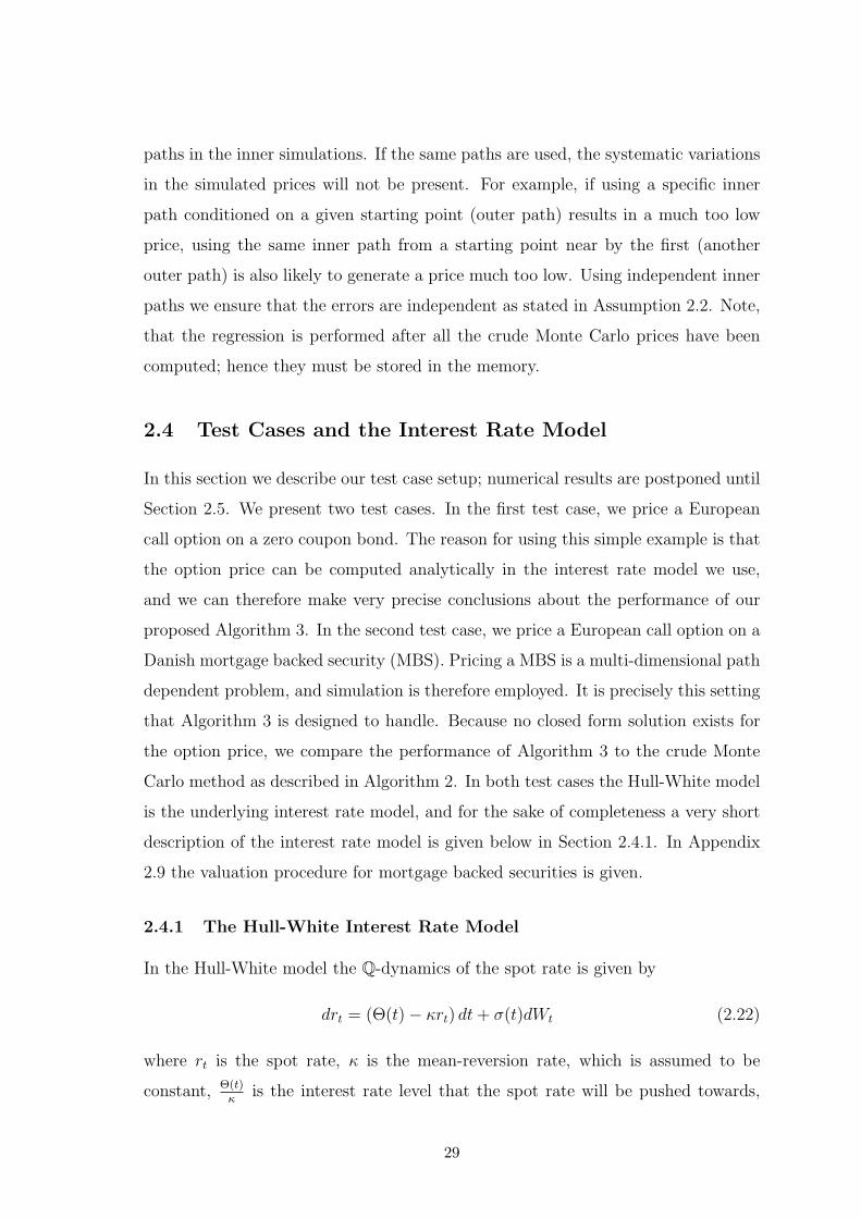
In Figure 2.5 the convergence of the simulated option price in the crude Monte Carlo

case is shown. Convergence is achieved for about 3000 outer simulations. However,

the uncertainty on the price of the underlying security results in an upward bias

on the option price, its size depending on the number of inner simulations used.

In the model with only 5 inner simulations, the option price converges to a price

36

much higher than the limit price, but as the number of inner simulations increase

the option price bias is reduced.

Figure 2.6 shows the convergence of simulated option prices when least squares

prices have been used to compute option pay-offs. Convergence is achieved for

approximately the same number of outer simulations as for crude Monte Carlo but

there is no upward option price bias. Even for the model with only 1 single inner

simulation, the least squares Monte Carlo method is able to come up with an option

price close to the limit price. With more than 3000 outer simulations used, the

number of inner simulations do not seem to have any major effect on the option

price. In that case all the models in Figure 2.6 produce option prices close to the

limit price. The exception is the model with only 1 inner simulation, which seems

to undervalue the true option price.

Besides reducing the option price bias, the least squares Monte Carlo approach

also gives lower variance on the option price estimate than crude Monte Carlo for

a low number of inner simulations. In Figure 2.7 the numerical difference between

standard deviations from crude Monte Carlo and least squares Monte Carlo are plot-

ted. For a small number of inner simulations the least squares Monte Carlo computed

option prices have lower variability than the crude Monte Carlo computed option

prices. As the number of inner simulations increases this difference diminishes.

2.5.4 Error Analysis

Each computed price shown in Figure 2.5 and 2.6 is the result of a single call to a

pricing routine. In order to study the error from the crude Monte Carlo and the

least squares Monte Carlo methods we have computed a sample of 50 independent

prices for each of the models. From these samples we compute the distribution of

the relative pricing error. Figures 2.8 and 2.9 show the result for the model with

400 outer simulations and 5 inner simulations - (400,5), and for the (12800,5) model.

The figures clearly demonstrate that the conclusions drawn from Figure 2.5 and 2.6

were not due to the paths used for those particular calculations. In general, not

surprisingly, the existence of many outer paths reduces the variance of the option

estimate for both algorithms. However, the option price computed with crude Monte

Carlo will converge to a wrong option price much higher than the limit price. For

37

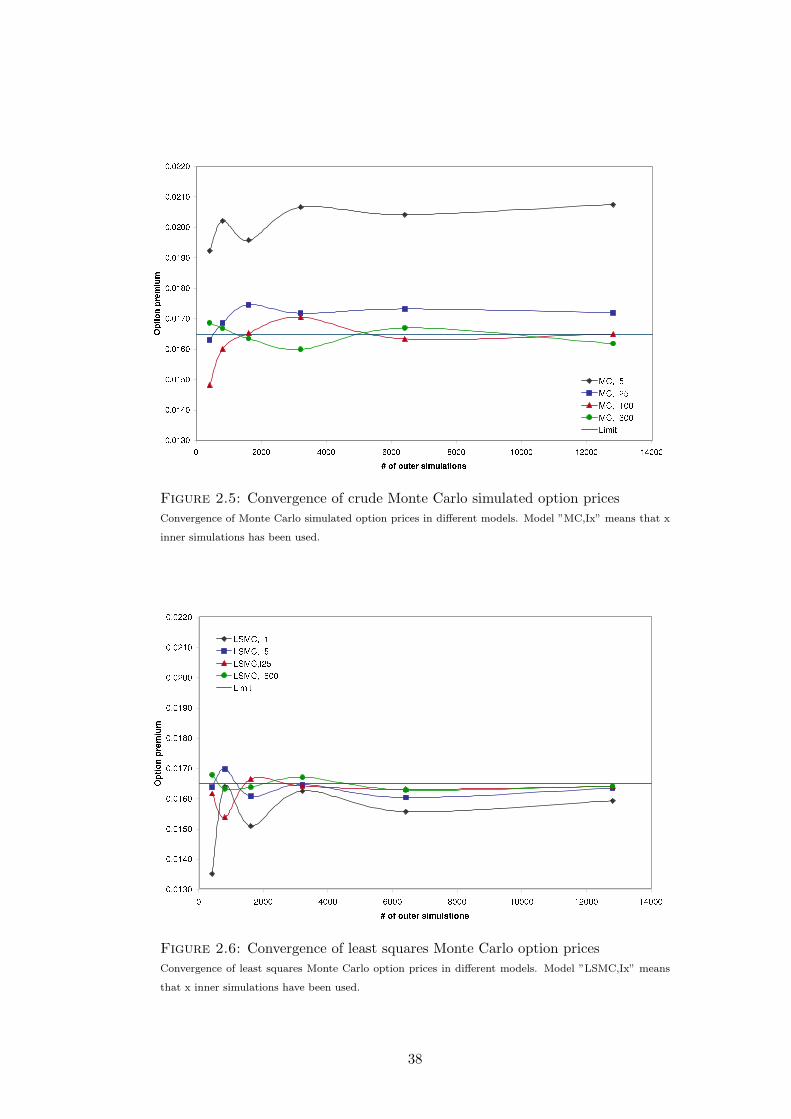
Figure 2.5: Convergence of crude Monte Carlo simulated option prices

Convergence of Monte Carlo simulated option prices in different models. Model ”MC,Ix” means that x

inner simulations has been used.

Figure 2.6: Convergence of least squares Monte Carlo option prices

Convergence of least squares Monte Carlo option prices in different models. Model ”LSMC,Ix” means

that x inner simulations have been used.

38

Figure 2.7: Differences in standard deviations

Differences in standard deviations between crude Monte Carlo and least squares Monte Carlo prices from

Figures 2.5 and 2.6.

400 outer simulations, about 12% of the least squares Monte Carlo computed option

prices have a relative pricing error of 0 and as many as 48% have a relative pricing

error below 5%. Option prices computed with crude Monte Carlo are all biased high

and none of the computed prices are within a 5% range of the true price. For 12800

outer simulations, approximately 54% have a relative pricing error of 0% using the

least squares method and 98% fall within a 5% range of the true price. In the case of

crude Monte Carlo, 12800 outer simulations result in convergence to a wrong price

much higher than the true price. None of the crude Monte Carlo simulated prices

are within a 5% range of the true price.

From the distributions of the relative pricing errors in different models, we have

calculated the probability of getting a relative pricing error below 5%. The results

are shown in Table 2.4. From the table a couple of interesting points can be made.

First, the result of Proposition 2.3 is very clear. Price estimates computed with

least squares Monte Carlo become closer to the limit price as the number of outer

simulations increases - the error distribution becomes more centered around 0. Also,

the least squares Monte Carlo prices do not depend so much on the number of inner

simulations in the sense that the number of outer simulations can always be increased

39

Figure 2.8: Histogram for the relative pricing error.

Histogram for the relative pricing error in the Crude Monte Carlo and least squares Monte Carlo case

using 400 outer and 5 inner paths. No other variance reduction methods are used. The probabilities are

found using a batch of size 50.

Figure 2.9: Histogram for the relative pricing error.

Histogram for the relative pricing error in the Crude Monte Carlo and least squares Monte Carlo case

using 12800 outer and 5 inner paths. No other variance reduction methods are used. The probabilities

are found using a batch size of 50.

40

in order for the price estimates to become more valid, i.e. into close range of the

limit price. In fact, for the calculations in Table 2.4, when more than 6400 outer

simulations are used no more that 25 inner simulations are needed in order to get

very precise option prices. Moverover, when using crude Monte Carlo it is crucial

to reduce the option price bias in order to get precise option prices. For very few

inner simulations crude Monte Carlo simulations cannot be used to produce a price

within an error margin of 5% of the limit price. In Appendix 2.9.4 the emperical

distribution function for the error term is shown for different models.

2.5.5 Efficiency Issues

As described in Section 2.3.2 least squares Monte Carlo is a crude Monte Carlo plus

a regression. The cost of performing the regression must therefore be lower than

the cost of the inner simulations saved, if least squares Monte Carlo is to be more

efficient than crude Monte Carlo. In Figure 2.10 we have graphed combinations of

outer and inner simulations that with 95% probability result in an absolute relative

pricing error below 5%. For a given number of inner simulations we have increased

the number of outer simulaitons until the probability of getting the wanted accuracy

has been achived.

In the least squares Monte Carlo method the number of inner simulations are 1,

5, 25, 50, 100, 200, 400 and 800. As suggested by Proposition 2.3 inner simulations

can be substituted by outer simulations. Few inner simulations require many outer

simulations to compensate for the high uncertainty in the price of the underlying

security. However, from an efficiency viewpoint, since many outer simulations also

incur higher computation time in the regression it might not be optimal just to

use few inner simulations. Looking at the least squares Monte Carlo computation

time in Figure 2.11 , we can see that it is optimal to have the number of inner

simulations below 25, which is also the minimum time used for achieving the desired

accuracy. With 25 inner simulations 4800 outer simulations are required to get the

desired accuracy with 95% probability. For this combination it takes 115 seconds5

to compute the option price.

In the crude Monte Carlo method only inner simulations from 50 to 800 have

5The calculations have been performed on a Pentium 4, 2.4 GHz, 512 MB RAM PC.

41

Table 2.4

Probability of |ǫ| ≤ 5%

Model#Outer #Inner LSMC MC

400 1 6% 0%800 1 14% 0%1600 1 8% 0%3200 1 40% 0%6400 1 78% 0%12800 1 96% 0%

400 5 48% 0%800 5 76% 0%1600 5 70% 0%3200 5 92% 0%6400 5 94% 0%12800 5 98% 0%

400 25 52% 52%800 25 60% 54%1600 25 88% 56%3200 25 90% 56%6400 25 100% 42%12800 25 100% 50%

400 50 56% 62%800 50 82% 68%1600 50 90% 84%3200 50 94% 90%6400 50 98% 90%12800 50 100% 100 %

400 100 52% 68%800 100 66% 78%1600 100 82% 92%3200 100 88% 98%6400 100 98% 100%12800 100 100% 100%

400 800 56% 62%800 800 78% 84%1600 800 84% 96%3200 800 90% 100%6400 800 100% 100%12800 800 100% 100%

Notes: The distributions are found on a 50 sample basis. #Outer and #Inner are the number of outerand inner paths respectively. No variance reduction has been used.

42

been computed. For fewer inner simulations it is not possible to compute an option

price within 5% of the limit price. For 50 inner simulations 9600 outer simulations

are needed but this number reduces to 2400 when 100 inner simulations are used.

This is also the most efficient combination of outer and inner simulations in the

crude Monte Carlo case. This combination of inner and outer simulations takes 133

seconds for computing an option price.

Figure 2.10: Outer/Inner trade-off.

Combinations of outer and inner simulations that with a probability of 95% results in an relative pricing

error below 5%. For a fixed number of inner simulations, the number of outer simulations is found using

interpolation between the number of simulations resulting in a probability just below and just above

95%. The sample size is equal to 50.

A measure that takes into account both the option price bias and the variance of

an estimator is the RMSE, which is defined as√

E[(c− c)2]. RMSE can therefore

be used to summarize, in a single number, the points drawn from Figure 2.7 and

Table 2.4. Using relative pricing errors as in (Broadie & Detemple, 1996), RMSE

can be estimated by the following formula, where J is the sample size.√

√

√

√

1

J

J∑

j=1

(

(cj − cj)

cj

)2

The traditional approach to compute RMSE is based on prices of contracts with

different specifications, i.e. different strikes, maturities etc. We, however, compute

it from the prices in the batches computed for estimating the distribution of the

43

Figure 2.11: Computation times.

Computation times found by interpolation from the models in Figure 2.10.

relative pricing error. The results are shown in Figure 2.12. The preferred region

is the upper-left corner, which combines high precision with high speed. As can be

seen the most efficient method to use in our test case is least squares Monte Carlo

with 5 inner simulations.

2.5.6 Result - Antithetic Sampling

6To see the impact on efficiency using antithetic sampling between today and option

expiry only, we have computed the same numbers presented in Table 2.4. The

numbers are shown in Table 2.5 below together with the number from Table 2.4.

Using antithetic sampling has a major positive effect on the least squares Monte

Carlo method. With only 5 inner simulations the number of outer simulations does

not have to be higher than 1600 in order to be almost certain to have an error within

a 5% range of the true price. Note that using antithtic sampling between today and

option expiry will not reduce the option price bias for crude Monte Carlo esitmates.

It that case only the variance in the option price will be reduced but the option price

bias will not.6Using antithetic sampling between today and option expiration is a violation of the conditions in

Equation (2.11) and Equation (2.12), but since the results are so promising we include them. The reason

for the violation is that antithetic paths are not independent.

44

Table 2.5

Probability of |ǫ| ≤ 5%

Model#Outer #Inner LSMC Antithetic LSMC

400 1 16% 6%800 1 6% 14%1600 1 50% 8%3200 1 76% 40%6400 1 94% 78%12800 1 100% 96%

400 5 88% 48%800 5 80% 76%1600 5 98% 70%3200 5 100% 92%6400 5 100% 94%12800 5 100% 98%

400 25 80% 52%800 25 96% 60%1600 25 98% 88%3200 25 100% 90%6400 25 100% 100%12800 25 100% 100%

400 50 82% 56%800 50 98% 82%1600 50 98% 90%3200 50 100% 94%6400 50 100% 98%12800 50 100% 100%

400 400 94% 56%800 400 97% 56%1600 400 98% 80%3200 400 100% 84%6400 400 100% 100%12800 400 100% 100%

400 800 92% 56%800 800 100% 78%1600 800 98% 84%3200 800 100% 90%6400 800 100% 100%12800 800 100% 100%

Notes: The distributions are found on a 50 sample basis. #Outer and #Inner are the number of outerand inner paths respectively. Antithetic sampling has been used between today and option expiry.

45

Figure 2.12: Speed-accuracy trade-off for different models.

RMS relative error is defined by√

1J

∑Jj=1((cj − cj)/cj)2, where cj is the true option value computed

by crude Monte Carlo with 64500 outer and 10000 inner paths and cj is either the crude Monte Carlo

or the least squares Monte Carlo estimate. Speed is measured as 1/(computation time in sec.). The

preferred region is the upper-left corner. The sample size, J , is equal to 50.

Of course, using antithetic sampling cannot be done without incurring additional

costs in the form of higher computation time. The efficiency of using least squares

Monte Carlo with antithetic sampling until option expiry is compared in Figure

2.13 with the least squares Monte Carlo without any variance reduction method.

The figure shows that using antithetic sampling considerably reduces the number of

outer simulations necessary for getting an error below 5% with a probability of 95%.

For more than 5 inner simulations the number of outer simulations are reduced by

a factor of two or more, indicating that antithetic sampling will indeed speed up

the method. This is also evident when looking at the computation times for the

two methods. The computation time for least squares Monte Carlo with antithetic

sampling is always below the computation time for the method without the variance

reduction technique. Least squares Monte Carlo with antithetic sampling is most

efficient for 25 inner simulations, in which case 775 outer simulations are necessary

to obtain an errror below 5% with 95% certainty. This only takes 35 seconds to

compute, whereas the most efficient set-up takes 115 seconds when no variance

reduction thechniques are used, yielding a speed-up factor of more than 3.

46

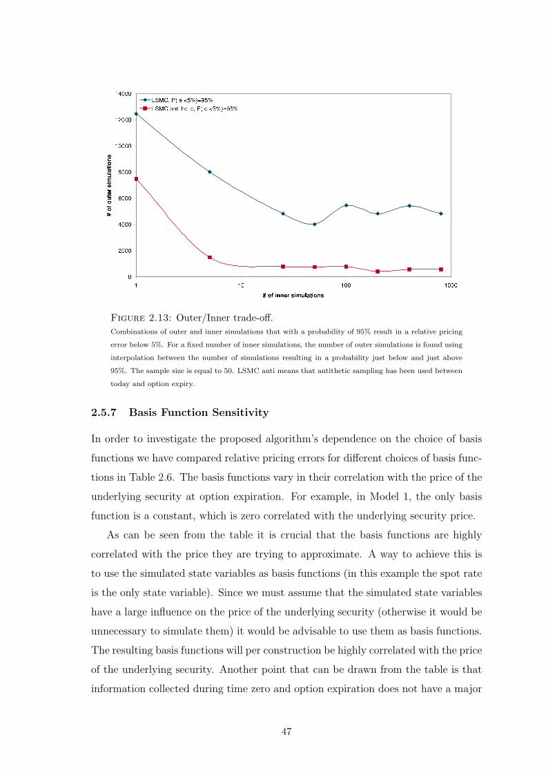
Figure 2.13: Outer/Inner trade-off.

Combinations of outer and inner simulations that with a probability of 95% result in a relative pricing

error below 5%. For a fixed number of inner simulations, the number of outer simulations is found using

interpolation between the number of simulations resulting in a probability just below and just above

95%. The sample size is equal to 50. LSMC anti means that antithetic sampling has been used between

today and option expiry.

2.5.7 Basis Function Sensitivity

In order to investigate the proposed algorithm’s dependence on the choice of basis

functions we have compared relative pricing errors for different choices of basis func-

tions in Table 2.6. The basis functions vary in their correlation with the price of the

underlying security at option expiration. For example, in Model 1, the only basis

function is a constant, which is zero correlated with the underlying security price.

As can be seen from the table it is crucial that the basis functions are highly

correlated with the price they are trying to approximate. A way to achieve this is

to use the simulated state variables as basis functions (in this example the spot rate

is the only state variable). Since we must assume that the simulated state variables

have a large influence on the price of the underlying security (otherwise it would be

unnecessary to simulate them) it would be advisable to use them as basis functions.

The resulting basis functions will per construction be highly correlated with the price

of the underlying security. Another point that can be drawn from the table is that

information collected during time zero and option expiration does not have a major

47

Table 2.6

Basis Function Sensitivity

Model Basis Fct. #Basis Fct. Error(400/50)

Error(6400/50)

1 1 1 -74.6% -100.0%2 1,r, r2 3 3.2% -0.4%3 1,r, r2, p, p2, rp 6 -0.2% -1.2%4 1,r, r2, ω1, ω

21, ω2

ω22, rω1, rω2, ω1ω2 10 -1.4% -1.8%

5 1,p, p2 3 -21.9% -23.8%6 1,p, p2, ω1, ω

21, ω2

ω22, pω1, pω2, ω1ω2 10 -6.4% -8.0%

7 1,ω1, ω21, ω2, ω

22, ω1ω2 6 -16.2% -17.3%

Notes: Errors relative to the price obtained by using 14 basis functions for the two models (400/50) and(6400/50).

impact on the pricing. In other words, at least for this example, the simulated state

variable alone is useful in explaining the price of the underlying security at option

expiration, meaning that the path dependent nature of the mortgage bond for a

large part is captured by observing the spot rate at the beginning and at option

expiration.

2.6 Improvements

In this paper we have reduced the option price bias by regressing the Monte Carlo

computed prices of the underlying security onto a set of basis functions. The most

important question here is how to create a precise regression. In this section we will

discuss a few ways to accomplish this and some complications that can arise when

trying.

2.6.1 Inner Versus Outer Paths.

The first and probably most obvious way to get a more precise regression is to

increase the number of outer paths which will result in more observations to use in

the regression. Another just as obvious choice is to increase the number of inner

paths which will create more precise observations to use in the regression.

It is not obvious which combination of (M,N) we should use. Is there an optimal

48

combination of outer and inner simulations? Of course such a combination will

depend on the problem at hand and the implementation. We will illustrate this

issue by continuing the example from Section 2.5.1.

(M1, N1) and (M2, N2) will be called time equivalent if cLS(M1, N1) and cLS(M2, N2)

have the same calculation time. In Figure 2.14 we have shown a set of time equiv-

alent pairs. Now, we are interested in finding the best combination among these

pairs.

Figure 2.14: Iso time line.

Combinations of outer and inner simulations, (M,N), yielding identical computation time.

There are different ways of comparing these combinations. In Figure 2.15 we have

shown the average and indicated ±2 standard deviations for the estimated option

prices for each combination.7 As we can see the standard deviation is much larger

for a high number of inner simulations, indicating that it is inefficient to use too

many inner simulations. It is not clear if there is any difference in the bias produced

by each combination. In order to take both bias and variation into account we have

estimated the probability that the error is less than both 1% and 5%. These numbers

are shown in Figure 2.16. Here, we can see that a combination of 5 inner and 5125

outer simulations seems to be optimal both for 1% and 5%.

In our MBS example from Appendix 2.9 the calculation of an inner path was

7We have used a sample of 50000 independent simulations to estimate averages and standard deviations.

49

Figure 2.15: Bias estimation for time equivalent pairs of inner and outer

simulations.

Figure 2.16: P(Error≤a) for time equivalent pairs of inner and outer simula-

tions.

50

far more complex than an outer path. This suggests that we should use fewer inner

paths for that type of problem. In that example the variance of the MBS estimates

is highly state dependent. Hence, we can improve the regression simply by using

more inner paths in the high variance regions. For the callable mortgage bond this

is around the time when people start to call the mortgage bond.

2.6.2 An Infinite Dimensional Set of Basis Functions.

In the previous sections we have assumed that the price of the underlying asset is

spanned by a finite set of basis functions. This is usually not the case. In Appendix

2.9 we valued an option on a callable mortgage bond which was not spanned by the

set of basis functions used in the regression.

To illustrate this type of problem we will again turn to our example from Section

2.5.1. In this example we know the price at the exercise time and can therefore

create a set of basis functions that will span the solution. How will this method

work if we do not know the true value? In Figure 2.17 we show for N = 5 and

M = 5000 the bias and ±2 standard deviations of the bias estimate. The series

labelled ”Polynomial” does not include the exponential function as a basis function

whereas the series labelled ”Incl. exp” does. Recall that if the exponential function

is included in the set of basis functions the true price will be spanned by the basis

functions. As can be seen, in the ”Polynomial” case, nothing is gained by having

more than 3 basis functions, so just increasing the number of basis functions to

beyond 3 will not produce better bias reduction. Note, that the bias created when the

exponential function is not included in the basis functions is greater than when it is

included. At first it might seem peculiar that we do not gain any more accuracy from

increasing the number of basis functions. The reason is that more basis functions

give more volatile coefficients for the same number of observations. Hence, in order

to get the same precision a higher number of observations is required. On the other

hand, too few basis functions will produce a functional form which is far from the

true functional form. (Glasserman & Yu, 2003) show that the number of outer

simulations needed grows exponentially with the number of basis functions. Hence,

more is not always better. For this reason it is very important to choose the best set

of basis functions for which a low-dimensional set of basis functions is acceptable.

51

Figure 2.17: Bias estimation for polynomial basis function.

2.6.3 Importance Sampling.

For a call option we are only interested in an accurate estimate above the strike. For

this reason we want to concentrate our regression on this region. This is important

both to get a more precise regression but also few basis functions will be better at

approximating a minor region. The simplest way of concentrating our regression on

the critical region is to exclude some observations from the regression. In Figure

2.18 we have excluded all observations of the zero coupon bond price from Section

2.5.1 where the true price is less than 0.5. As we can see the regression is shifted to

the right.

This reduces the bias significantly as can be seen from comparing Figure 2.19

with Figure 2.17 where the only difference is the sample used in the regression.

This is a very extreme way of focusing the regression. Another way is to use

importance sampling. This is a well-documented variance reduction technique which

is used to create more samples of the state variables in the most critical regions. This

technique can be used to increase the number of samples in the most volatile areas

instead of increasing the number of inner paths in the same areas.

52

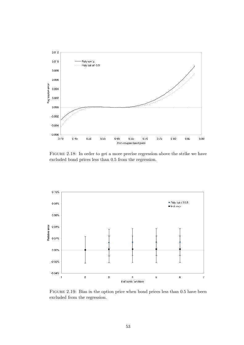
Figure 2.18: In order to get a more precise regression above the strike we have

excluded bond prices less than 0.5 from the regression.

Figure 2.19: Bias in the option price when bond prices less than 0.5 have been

excluded from the regression.

53

2.7 Conclusion

In this paper we have developed a method to reduce the option price bias in the Eu-

ropean option price, resulting from using simulated prices of the underlying security

when computing option pay-offs. We have shown that in an ideal world where the

true price is spanned by a set of basis functions the option price bias can be com-

pletely removed by increasing the number of outer simulations independent of the

number of inner simulations. Under the same assumptions, we have also shown that

the least squares estimate of the price of the underlying security has lower variance

than the crude Monte Carlo estimate leading to lower option price bias.

Even when the true price is approximated by a finite linear combination of the

basis functions, i.e. the true price does not belong to the space spanned by the basis

functions, we have seen in a numerical example that the least squares computed

option price converges to the limit price as the number of outer simulations increases.

For a single inner simulation we were able to compute an option price very close to the

limit price using many outer simulations. The method can also be viewed as a way

to substitute inner simulations with outer simulations. This is particularly efficient

when the cost of simulating inner paths is high compared to the cost of simulating

outer paths as in the case of pricing short-term options on long-lived securities.

In our computational test case the least squares Monte Carlo method proved to be

faster than crude Monte Carlo when no other variance reduction methods were used.

We also demonstrated that the bias reduction method can be combined with

other variance reduction techniques. In Section 2.6 it was shown that the regression

could be considerably improved by focusing on the relevant region as is done in

important sampling. In Section 2.5.6 antithetic sampling between today and option

expiry was employed to improve the regression. Compared to the case with no

variance reduction techniques we obtained a speed-up factor of three by using the

least squares Monte Carlo method.

54

2.8 Appendix A: Proofs

2.8.1 Proof of Proposition 2.1

We first show that option prices are upwardly biased when option pay-offs are com-

puted using the prices of the underlying security that contain a noisy element.

ct = EQt

[

e−∫ T

trs dsf (PT , K)

]

= EQt

[

e−∫ T

trs dsf

(

EQT

[

PT

]

, K)]

≤ EQt

[

e−∫ T

trs dsE

QT

[

f(

PT , K))]]

= EQt

[

e−∫ T

trs dsf

(

PT , K)]

= ct

The first equality comes from the general pricing formula for pricing under the risk

neutral probability measure. In the second equality PT is an unbiased estimator of

the true price of the underlying security, PT . The third line follows from Jensen’s

inequality and the convexity of the pay-off function f(P,K). In the fourth line we

use the the law of iterated expectations and the fifth equality is given by definition.

Next we show that the option price bias can be controlled by determining an

upper bound on the deviation from the true price of the underlying security.

ct = EQt

[

e−∫ T

trs dsf (PT + ǫ, K)

]

≤ EQt

[

e−∫ T

trs ds (f (PT , K) + |ǫ|)

]

= EQt

[

e−∫ T

trs dsf (PT , K)

]

+ EQt

[

e−∫ T

trs ds |ǫ|

]

= ct + EQt

[

e−∫ T

trs dsE

QT

[√ǫ2]]

≤ ct + EQt

[

e−∫ T

trs ds]

√

VarQt [ǫ]

= ct + σǫEQt

[

e−∫ T

trs ds]

The first equality follows from Equation (2.4). The second line follows from moving

ǫ out of the pay-off function, and using the anatomy of the pay-off function. In the

third line we use the linearity of the expectation operator. The fourth equality fol-

lows from the definition of the true option price and the law of iterated expectations.

Then we use Equation (2.5) and Jensen’s inequality to interchange the E operator

and the√· function. Finally we use Equation (2.6).

55


The first statement of the proposition follows by

EQT

[

PLST

]

= EQT

[

Lb]

= LEQT

[

b]

= Lb = PT

where the first equality follows from (2.16), the second equality follows from L being

T -measurable, the third equality follows from the unbiasedness of the estimator b

as stated in (2.15) and the last equality follows from Assumption 2.1. The second

statement is proved by

VarQT

[

PLS,iT

]

= VarQT

[

Lib]

= LiVarQT

[

b]

(Li)T

= σ2ǫ Li (LTL)

−1(Li)T

The first equality is given by (2.16), the second follows from moving the vector Li

out of the variance operator, and in the third equality we use Equation (2.15).

If Li (LTL)−1

(Li)T ≤ 1 the result is proved. To confirm that this is the case

we use a corollary of the extended Cauchy-Schwartz inequality (see (Johnson &

Wichern, 1998) page 82), which states

maxx 6=0

(xTd)2

xTBx= dTB−1d (2.25)

where B is a positive definite matrix and d and x are vectors.

We will use this result with d = (Li)T and B = LTL. Note, that both the nomina-

tor and denominator are scalars and can be evaluated separately. The denominator

is equal to

xT(LTL)x = (Lx)T (Lx)

=M∑

k=1,k 6=i

(

Lkx)2

+(

Lix)2

(2.26)

The nominator is equal to

(

xT(Li)T)2

=(

Lix)2

(2.27)

56

hence, by inserting (2.26) and (2.27) into (2.25) we can conclude that

Li(LTL)−1(Li)T ≤ 1 ∀ i

from which the the result follows.


From Proposition 2.1 we know that cLSt ≤ ct +E

Qt

[

e−∫ T

trs ds]

√

VarQt [ǫLS]. If we can

show that the last term approaches 0 as the number of outer simulations M increases

we have shown (2.20). In the proof of Proposition 2.2 we saw that VarQT

[

PLS,iT

]

=

σ2ǫL

i (LTL)−1

(Li)T. Now,

VarQt

[

ǫLS,i]

= VarQt

[

EQT

[

ǫLS,i]]

+ EQt

[

VarQT

[

ǫLS,i]]

= EQt

[

VarQT

[

PLS,iT

]]

= EQt

[

σ2ǫL

i (LTL)−1

(Li)T

]

=σ2

ǫ

ME

Qt

[

LiQ−1M (Li)T

]

→ 0 as M → ∞ ∀ i

The first equality can be found in e.g. (Greene, 2002), page 866, the second and

third lines follow from Assumption 2.2 and PLS,iT = PT + ǫLS,i

T . The result follows

now from Assumption (2.19).

57

2.9 Appendix B: MBS Valuation

In this section we will briefly describe pricing of mortgage backed bonds by simula-

tions. We also give an example showing the intuition in using least squares Monte

Carlo estimates for computing option pay-offs when few inner simulations are em-

ployed.

A callable mortgage bond gives the borrower the right to prepay the remaining

loan balance at any point in time. However, debt holders do not follow the optimal

exercise strategy which excludes the use of traditional option theory in the valuation

of the borrower side. Instead, a statistical model is used, which over time explains

the majority of the variations in prepayments across different mortgage pools. The

prepayment function must take into account heterogeneity among borrowers as a

result of a long issue period8and behavioural differences among debt holders for

utilizing the prepayment option. Many models use the after tax and costs9 gain from

refinancing as one of the explanatory variables. The value of this variable captures

prepayments arising from future market situations. However, as the mortgage pool

characteristics change because the most inclined prepayers leave the mortgage pool,

a given level of refinancing gains tends to result in lower prepayments than when

the level was hit the first time. To capture this and dampen prepayments in series

that have already experienced prepayments, (Jakobsen, 1994) suggests dividing the

mortgage pool into tranches, each with its own prepayment function. This will

capture some divergences in prepayments among debtor groups over time, because

when the pool changes from large to small loans, prepayments will fall. However,

we find that a combination of this method and a more direct modelling of the

burnout gives a better explanation of variations in prepayments. The model we use

thus utilizes the series pool factor as a way to capture additional burnout among

debt holders. See (Schwartz & Torous, 1989) and (Jakobsen, 1992) for an in-depth

description of prepayments and valuation of MBS’.10

8In Denmark callable mortgage bonds are open for issue for up to three years, which means that the

same underlying pool of mortgage bonds can be issued to borrowers under very different market conditions.9The costs of refinancing are: DKK 2500 in fixed costs, 2.5% in differential rate, 1% in creation fee and

0.15% in brokerage fee.10(Jakobsen, 1992) is the main reference for valuation of Danish callable mortgage bonds.

58

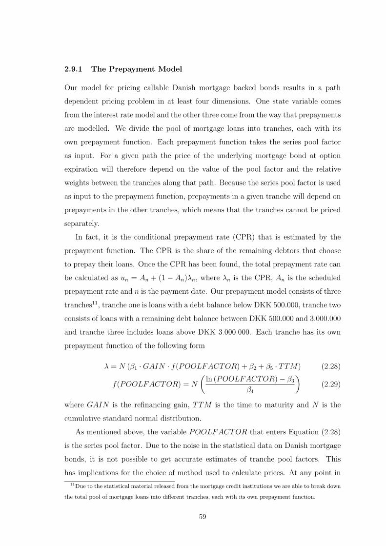
2.9.1 The Prepayment Model

Our model for pricing callable Danish mortgage backed bonds results in a path

dependent pricing problem in at least four dimensions. One state variable comes

from the interest rate model and the other three come from the way that prepayments

are modelled. We divide the pool of mortgage loans into tranches, each with its

own prepayment function. Each prepayment function takes the series pool factor

as input. For a given path the price of the underlying mortgage bond at option

expiration will therefore depend on the value of the pool factor and the relative

weights between the tranches along that path. Because the series pool factor is used

as input to the prepayment function, prepayments in a given tranche will depend on

prepayments in the other tranches, which means that the tranches cannot be priced

separately.

In fact, it is the conditional prepayment rate (CPR) that is estimated by the

prepayment function. The CPR is the share of the remaining debtors that choose

to prepay their loans. Once the CPR has been found, the total prepayment rate can

be calculated as un = An + (1 − An)λn, where λn is the CPR, An is the scheduled

prepayment rate and n is the payment date. Our prepayment model consists of three

tranches11, tranche one is loans with a debt balance below DKK 500.000, tranche two

consists of loans with a remaining debt balance between DKK 500.000 and 3.000.000

and tranche three includes loans above DKK 3.000.000. Each tranche has its own

prepayment function of the following form

λ = N (β1 ·GAIN · f(POOLFACTOR) + β2 + β5 · TTM) (2.28)

f(POOLFACTOR) = N

(

ln (POOLFACTOR) − β3

β4

)

(2.29)

where GAIN is the refinancing gain, TTM is the time to maturity and N is the

cumulative standard normal distribution.

As mentioned above, the variable POOLFACTOR that enters Equation (2.28)

is the series pool factor. Due to the noise in the statistical data on Danish mortgage

bonds, it is not possible to get accurate estimates of tranche pool factors. This

has implications for the choice of method used to calculate prices. At any point in

11Due to the statistical material released from the mortgage credit institutions we are able to break down

the total pool of mortgage loans into different tranches, each with its own prepayment function.

59

the future, the series pool factor must be calculated as a weighted average of the

tranche pool factors (see Equation (2.31) below). However, this requires knowledge

of all the tranche weights simultaneously. Additional state variables comes from

the interest rate model. We therefore use Monte Carlo simulations when pricing

Danish mortgage backed bonds. If a PDE solution were to be used, we would have

to augment the state space with the number of tranches, and with a total of more

than four state variables, the PDE approach would be unmanageable. In (Paskov,

1996), a similar pricing problem is presented although he prices different tranches

of a CMO on a pool of mortgage loans instead of the mortgage pool itself.

2.9.2 Updating Rules

Along a given path, variables influencing the option pay-off must be updated. In the

case of options on MBS, variables that determine the bond price must be updated

between today and option expiration. The variables are the pool factor and the

relative tranche weights, which summarizes changes in debtor distribution.

The pool factor for tranche k at date n measures how much debt is left in the

tranche at time n. Knowing the tranche size relative to the series size at time 0 and

prepayments in the tranche between 0 and n, the pool factor of the tranche at time

n can be calculated as

pkn = p0ω

k0

n∏

j=1

(

1 − λkj

)

(2.30)

where p0 is the series pool factor at time 0, ωk0 is the tranche weight for tranche k

at time 0 and λkj is the cpr rate for tranche k at time j. The series pool factor at

date n can be found by

pn =K∑

k=1

pkn (2.31)

where K is the number of tranches.

The tranche weights are defined as the tranche size relative to the whole series

and are given by

ωkn =

p0ωk0

∏nj=1

(

1 − λkj

)

∑

k p0ωk0

∏nj=1

(

1 − λkj

) =pk

n

pn

(2.32)

60

Notice that the tranche weights add to unity.

K∑

k=1

ωkn = 1

2.9.3 Monte Carlo Formulation of MBS Valuation Problem

Let bkn be the payment from tranche k at payment date n. It can be computed as

bkn =n−1∏

j=1

(1 − λkj )(

λknH

kn + (1 − λk

n)Akn + Ik

n

)

(2.33)

where Akn, Ik

n are the scheduled prepayment and interest payment from tranche k at

payment date n respectively and Hkn is the scheduled remaining debt balance at pay-

ment date n before a redemption payment is made. Note that when the prepayment

function depends on previously computed λ’s, bkn will be path dependent12.

Using (2.3) we find the value of a single payment as

Vt(bkn) = E

Qt

[

bkne−∫ Tn

trs ds]

where Tn is the payment date. Let V mt (k) be an estimate of the MBS value along

path m. With N payment dates the price of tranche k at time t along path m is

given by the sum of the prices of the individual payments along that path

V mt (k) =

N∑

n=1

V mt (bkn)

The crude Monte Carlo estimate of the value of tranche k is therefore given by

Vt(k) =1

M

M∑

m=1

V mt (k)

and the price of the total pool of mortgage loans is computed as a weighted sum of

the prices of each of the tranches, times the tranche weights.

Vt(MBS) =K∑

k=1

ωk0 Vt(k) (2.34)

12It is precisely these λ’s that depend on the series pool factor, and the value of the tranche weights

must thus be known simultaneously.

61

2.9.4 An Example

To illustrate how least squares can be used to reduce the bias, we have plotted

95% confidence intervals for future MBS prices calculated with and without least

squares. The prices are computed using 400 outer paths and 5, 50 and 500 inner

paths respectively. No other variance reduction methods are used. The future

trading date is July, 1, 2004 using data from January, 9, 2003. The results are

shown in Figures 2.20, 2.21 and 2.22. The x-axis shows the future spot rates and

the y-axis shows the simulated prices given the future state for a principal of DKK

1. The light gray lines are prices calculated without using the least squares approach

and the black lines are calculated using least squares. Some of the variation in the

figures can be explained by differences in vaiables like the pool factor and the debtor

distribution, which is why the regressed expression is not a smooth function. In

Figure 2.23 the corresponding spot rate distribution at option expiration is shown.

With only five inner paths the MC prices are, not surprisingly, extremely volatile.

The maximum difference between the upper and lower bound in the confidence

interval is as large as DKK 0.25 meaning that another simulation could result in a

price DKK 0.25 away from the calculated price given the same state. Running a

least squares regression, however, has a remarkable effect on the confidence interval.

The maximum distance between the upper bound and the lower bound narrows to

DKK 0.07 and if we only look at spot rates between 1% and 5%, the maximum

difference declines to DKK 0.04. Results from increasing the number of inner paths

to 50 are shown in Figure 2.21. As expected the MC price estimates becomes much

less volatile compared to the prices in Figure 2.20. The maximum distance between

the upper and lower bound in the confidence interval without using least squares is

DKK 0.06 and only DKK 0.03 when a regression is applied. Finally, increasing the

number of inner paths to 500 yields almost identical confidence intervals for the two

methods. The maximum distance now falls to DKK 0.02 in the crude Monte Carlo

case and to DKK 0.007 in the case where least squares is used. It is worth noting

that even in the case of 500 inner paths the crude Monte Carlo confidence band is

still not as good as the band obtained using least squares. In fact, in this example, it

seems that the maximum distance between the upper and lower bounds declines with

the same factor in both cases when the number of inner paths increases suggesting,

62

that it is always worthwhile to run a regression. For very low rates, however, there is

large difference between the crude Monte Carlo prices and the prices obtained from

least squares. The reason is that there are only few observations in this area making

the regression bad.

In the regressions used above, all the simulated prices have been used. This

approach can be refined. To improve the regression in areas which are important,

for example in areas where the option is in the money, the regression could be

performed using mostly in the money data.

63

Figure 2.20: 95% confidence intervals for MBS prices at option expiration

Crude Monte Carlo and least squares Monte Carlo prices for the underlying security at option expiration

using 400 outer and 5 inner paths. No other variance reduction methods are used. The standard deviation

of the least squares Monte Carlo estimate is found using 20 batches.



using 400 outer and 50 inner paths. No other variance reduction methods are used. The standard

deviation of the least squares Monte Carlo estimate is found using 20 batches.

64



using 400 outer and 500 inner paths. No other variance reduction methods are used. The standard

deviation of the least squares Monte Carlo estimate is found using 20 batches.

Figure 2.23: Spot rate distribution at option expiration

The distribution is found from the simulated spot rates associated with the least squares Monte Carlo

simulation in the figures above, i.e. from 400 simulations.

65

(a) (400,25) (b) (800,25)

(c) (1600,25) (d) (3200,25)

(e) (6400,25) (f) (12800,25)

Figure 2.24: Empirical cumulative distribution functions

Cumulative distribution functions for the relative pricing error in the models (Outer, Inner). The distri-

butions are found on a 50 sample basis.

66

2.10 Appendix C: MBS Computational Test Case

Table 2.7

Basic bond data

Parameter Value

Isin code DK¡0009265076Coupon rate 6%

Maturity 01/10/2032Payments per year 4

Amortization AnnuityInitial pool factor 0.97Tranche weight 1 0.15Tranche weight 2 0.75Tranche weight 3 0.10

The parameter values for the prepayment model used in this paper are given in

Table 2.8 below.

Table 2.8

Basic bond data

Parameter Tranche 1 Tranche 2 Tranche 3

β1 0.15 0.20 0.25β2 -1.60 -1.00 -0.60β3 -4.20 -3.40 -2.50β4 1.80 1.20 0.80β5 -0.05 -0.10 -0.15

Parameters in the interest rate model are calibrated to be as shown in Table 2.9.

Table 2.9

Basic bond data

Parameter Value

κ 0.03σ2

0−0.25 0.01σ2

0.25−5 0.009σ2

5−10 0.008σ2

10− 0.007

67

Chapter 3

An Algorithm for Simulating

Bermudan Option Prices on

Simulated Asset Prices

Co-authored with Brian Huge, Danske Bank

68

Abstract

In this paper we present an algorithm that combines the (F. Longstaff & Schwartz,

2001) simulation algorithm and the bias reduction technique developed in (Huge &

Rom-Poulsen, 2004) to simulate Bermudan option prices on securities so complex

that their price must be found by Monte Carlo simulations. Bias reduction is needed

because using simulated prices of the underlying security to compute option pay-offs

causes an upward bias in the option price. We prove consistency of the option price

computed by the algorithm.

69

3.1 Introduction

In this paper we use the (F. Longstaff & Schwartz, 2001) simulation algorithm to

price Bermudan options written on securities so complex that their price must be

computed by Monte Carlo simulations. In recent years, approximation methods for

pricing Bermudan style options by Monte Carlo simulations have been developed.

The first attempts to price Bermudan style options by Monte Carlo simulations were

done in (Tilley, 1993) and (Carriere, 1996). Recently, several other methods have

been proposed. These include (F. Longstaff & Schwartz, 2001) and (Tsitsiklis &

Van Roy, 2001), the random tree method in (Broadie & Glasserman, 1997) and the

stochastic mesh method of (Broadie & Glasserman, 2004), state space partitioning

as in (Barraquand & Martineau, 1995) and the dual method in (Rogers, 2002). A

survey of American option pricing using Monte Carlo simulations can be found in

(Fu, Laprise, Madan, Su, & Wu, 2001) and chapter 8 in (Glasserman, 2004).

Not much attention has been given to the problem of pricing Bermudan options

on securities that themselves must be priced by simulations. Although the theoret-

ical problem is already covered by the methods above, the additional problem of

simulating the price of the underlying security increases the computational burden

considerably. In this paper we show that this does not have to be the case. To the

best of our knowledge, this paper is the first to address this particular problem.

All the above mentioned methods use dynamic programming to solve the in-

herited maximization problem that must be solved in order to compute the price

of a Bermudan option. Since the maximum is taken over all stopping times, dy-

namic programming is essentially used to find the optimal exercise policy for the

option. The procedure is as follows; first, the state space is simulated using a (in

time) forward running routine. Secondly, the dynamic programming is solved using

a backward running routine. The backward running routine is a recursive procedure

that is initialized at option expiration by setting the option value equal to the option

pay-off. It then recursively works back to time 0 by, at each exercise date, setting

the option value equal to the maximum of the immediate exercise value and the

present value of the expected future option value, also known as the continuation

value. I.e. at each exercise date a decision is made whether to exercise the option

70

or to hold it for another period.

To use the dynamic programming approach, it is therefore necessary to be able to

compute option pay-offs at each exercise date. However, if the price of the underlying

security must be computed by simulations, the problem of computing option pay-

offs poses a huge computational burden. For example, consider a Bermudan option

with L exercise dates. Using U paths to simulate the state space and N paths to

simulate prices of the underlying security at each exercise date results in a total of

L× U ×N path generations of the underlying security. However, by using the bias

reduction technique in (Huge & Rom-Poulsen, 2004), the number of simulations used

to compute the price of the underlying security, N , can be reduced considerably. In

fact, it is shown that using one single simulation, N = 1, can be sufficient to find

prices of the underlying security and still get acceptable option pay-offs. However,

the number of state space simulations, U , must increase if N is to be low and a good

functional relationship between the price of the underlying security and the state

variables has to be established. We utilize this to develop a simulation algorithm

that prices Bermudan options on complex securities.

Section 3.2 contains the model setup. The dynamic programming principle is pre-

sented for the original Bermudan pricing problem and for the Least-Squares Monte

Carlo approximation. In addition we introduce our proposed extension, constructed

to handle cases in which the value of the underlying security must be found by Monte

Carlo simulations. In Section 3.3, our numerical test cases are presented along with

a short description of the Hull-White interest rate model. An explicit expression for

a class of basis functions in the Hull-White model is also developed for a bullet loan.

Section 3.4 contains the results of the test cases. Finally, conclusions are made in

Section 3.5.

3.2 The Model

Define a time line S = s0, s1, . . . , sM and let Xs0 , Xs1 , . . . , XsMbe a Rd-valued

Markov chain with Xs0 fixed. Xsi, i = 1, . . . ,M , represents the state variables which

must be simulated and upon which the underlying security depends. S contains both

71

exercise dates and dates influencing the future price of the underlying security1. It is

necessary to include non-exercise dates in S because, for path dependent securities,

variables that are important for the underlying security, may need to be updated

between exercise dates for future option pay-off computations to be possible. We also

define T = t0, t1, . . . , tL ⊆ S, t0 = s0 and tL < sM , as the set of stopping times. tL

is the expiration date of the option. We take as given a complete probability space(

Ω,F , FsiM

i=0,Q)

, where the discrete time filtration is generated by the relevant

processes in the economy. We assume that an equivalent martingale measure Q

exists under which all expectations are computed. Let hti(Xti), ti ∈ T be the t0

value of the pay-off at time ti. Since the pay-off function only influences the option

value on exercise dates, we put hsi(Xsi

) = 0 for all non-exercise dates si ∈ S. This

formulation of including the discounting into the pay-off function is discussed in

(Glasserman, 2004) section 8.1. To lighten notation, we let the subscript i indicate

time index ti or si.

3.2.1 Bermudan Option Pricing and Optimal Stopping

In this section we present the original Bermudan option pricing problem in which

no approximations are made. The Bermudan option price is given as the value

of the option if optimal exercise behaviour is followed by the holder of the option

(see (Duffie, 1996)). The optimal exercise strategy amounts to choosing the time of

exercise (stopping time) that maximizes the value of the option today. Let V ∗i (Xi)

denote the value of the option at exercise date ti ∈ T in state Xi. The superscript ∗

indicates that this is the option price in the problem where no approximations are

made. The value of the option is found by choosing, from the set of stopping times

Ti = i, i+ 1, . . . , L, τ ∈ Ti that maximizes V ∗i (Xi). I.e.

V ∗i (Xi) = max

τ∈Ti

EQi [hτ (Xτ )] (3.1)

V ∗i (Xi) is the value of the option given that the option was not exercised before

date ti. We are interested in computing V ∗0 (X0), the value of the option today. The

1Such dates could for example be payment dates of a callable mortgage backed bond, which will influence

future values of the bond, because future payments from the bond might be dependent on historical

prepayments.

72

optimal stopping time is found using dynamic programming, and V ∗0 (X0) is found

recursively as follows:

V ∗L (XL) = hL(XL) (3.2)

V ∗i (Xi) = max

(

hi(Xi),EQi [V ∗

i+1(Xi+1)])

, ti ∈ T , i < L (3.3)

At option expiration the value of the option is equal to its exercise value given by

the function hL(XL). An any exercise date i before expiration, the option holder

has to decide whether to hold the option for another period, which has the value

EQi [V ∗

i+1(Xi+1)], or to exercise immediately yielding a pay-off of hi(Xi). Working

backwards iteratively, this procedure gives the solution to the pricing problem in

Equation (3.1).

The Bermudan option valuation problem can also be formulated using continu-

ation values. Define

C∗i (Xi) = E

Qi [V ∗

i+1(Xi+1)] (3.4)

and the recursion procedure in (3.2) and (3.3) now becomes

C∗L(XL) ≡ 0 (3.5)

C∗i (Xi) = E

Qi [V ∗

i+1(Xi+1)] , ti ∈ T , i < L (3.6)

V ∗i (Xi) = max (hi(Xi), C

∗i (Xi)) , ti ∈ T (3.7)

Obviously, the continuation value is 0 at option expiration. At any date before

option expiration, the continuation value is equal to the present value of the expected

option value one period ahead. The option value is then given as the maximum of

immediate exercise and the continuation value.

As can be seen from (3.2) and (3.3) or (3.5), (3.6) and (3.7), the dynamic pro-

gramming routine works backward in the time dimension, and solving it using a

forward working Monte Carlo simulation therefore seem impossible. However, in

recent years, methods that combine Monte Carlo simulations and the dynamic pro-

gramming problem have been proposed.

3.2.2 Least Squares Monte Carlo Simulations (LSMC)

In order to distinguish approximated functions from functions from the original

problem presented in Section 3.2.1, we will use the notational convention that ap-

73

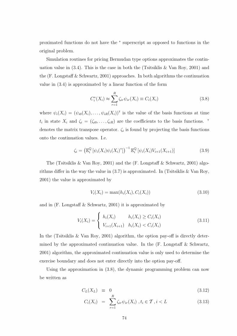
proximated functions do not have the ∗ superscript as opposed to functions in the

original problem.

Simulation routines for pricing Bermudan type options approximates the contin-

uation value in (3.4). This is the case in both the (Tsitsiklis & Van Roy, 2001) and

the (F. Longstaff & Schwartz, 2001) approaches. In both algorithms the continuation

value in (3.4) is approximated by a linear function of the form

C∗i (Xi) ≈

R∑

r=1

ζirψir(Xi) ≡ Ci(Xi) (3.8)

where ψi(Xi) = (ψi0(Xi), . . . , ψiR(Xi))T is the value of the basis functions at time

ti in state Xi and ζi = (ζi0, . . . , ζiR) are the coefficients to the basis functions. T

denotes the matrix transpose operator. ζi is found by projecting the basis functions

onto the continuation values. I.e.

ζi =(

EQi [ψi(Xi)ψi(Xi)

T])−1

EQi [ψi(Xi)Vi+1(Xi+1)] (3.9)

The (Tsitsiklis & Van Roy, 2001) and the (F. Longstaff & Schwartz, 2001) algo-

rithms differ in the way the value in (3.7) is approximated. In (Tsitsiklis & Van Roy,

2001) the value is approximated by

Vi(Xi) = max(hi(Xi), Ci(Xi)) (3.10)

and in (F. Longstaff & Schwartz, 2001) it is approximated by

Vi(Xi) =

hi(Xi) hi(Xi) ≥ Ci(Xi)

Vi+1(Xi+1) hi(Xi) < Ci(Xi)(3.11)

In the (Tsitsiklis & Van Roy, 2001) algorithm, the option pay-off is directly deter-

mined by the approximated continuation value. In the (F. Longstaff & Schwartz,

2001) algorithm, the approximated continuation value is only used to determine the

exercise boundary and does not enter directly into the option pay-off.

Using the approximation in (3.8), the dynamic programming problem can now

be written as

CL(XL) ≡ 0 (3.12)

Ci(Xi) =R∑

r=1

ζirψir(Xi) , ti ∈ T , i < L (3.13)

74

and Vi(Xi) equal to either (3.10) or (3.11).

In the rest of the paper we will focus on the (F. Longstaff & Schwartz, 2001)

algorithm only.

3.2.3 Extension of the LSMC Method

As dictated by the dynamic programming routine we must be able to compute the

immediate exercise value hi(Xi). When the price of the underlying security itself

must be computed by simulations, an additional approximation is made. In that

case, the option pay-off hi(Xi) is replaced by the approximation

hi(Xi) = f(

Pi(Xi))

(3.14)

where Pi(Xi) is the price estimate of the underlying security in stateXi and f(Pi(Xi))

is the pay-off function for a call/put taking as input the state dependent price of

the underlying security at exercise date ti. Pi(Xi) could be a crude Monte Carlo

estimate, but as shown in (Huge & Rom-Poulsen, 2004) this creates a bias in the

option price. To reduce this bias much computational effort has to be allocated to

find P (Xi). (Huge & Rom-Poulsen, 2004) propose an alternative price estimator

for the price of the underlying security. This estimator uses crude Monte Carlo

estimates to construct a new estimator that is less dependent of the computational

effort put into generating the crude Monte Carlo estimates. The study in (Huge

& Rom-Poulsen, 2004) only considers European options but in this section their

arguments are extended so that the bias reduction method can be applied to price

Bermudan options as well.

We will make the following assumptions:

Assumption 3.1 Assume that the true price of the underlying security, Pi, ti ∈ T ,

is given as a finite linear combination of V basis functions. I.e.

Pi(Xi) =V∑

v=1

υivφiv(Xi) (3.15)

Assumption 3.2 For each exercise date ti ∈ T , along any two paths m,n, an

unbiased crude Monte Carlo estimate, with independent error terms, for the price

75

of the underlying security can be computed. I.e.

PMC,ni (Xi) = Pi(Xi) + ǫMC,n

i (3.16)

EQi

[

ǫMC,ni

]

= 0 (3.17)

VarQi

[

ǫMC,ni

]

= σ2ǫ (3.18)

CovQi

[

ǫMC,mi , ǫMC,n

i

]

= 0 , ∀m,n (3.19)

If Assumptions 3.1 and 3.2 are fulfilled, a better estimate for the price of the

underlying security is given by

PLSi (Xi) =

V∑

v=1

υivφiv(Xi) (3.20)

where υi = (υi1, . . . , υiV )T is computed by

υi =(

EQi [φi(Xi)φi(Xi)

T])−1

EQi

[

φi(Xi)PMCi (Xi)

]

(3.21)

I.e. given Assumption 3.1 and Assumption 3.2, noise is removed by projecting the

crude Monte Carlo estimates of the price of the underlying security onto a set of

basis functions.

We denote functions that use the approximations (3.14) and (3.20) by superscript

LS. The dynamic programming problem can now be stated as

CLSL (XL) ≡ 0 (3.22)

CLSi (Xi) =

R∑

r=1

ζLSir ψir(Xi) , ti ∈ T , i < L (3.23)

V LSi (Xi) =

hLSi (Xi) , hLS

i (Xi) ≥ CLSi (Xi) , ti ∈ T , i < L

V LSi+1(Xi+1) , hLS

i (Xi) < CLSi (Xi) , ti ∈ T

(3.24)

with hLSi (Xi) = f(PLS

i (Xi)) and PLSi (Xi) given by (3.20).

3.2.4 Solving with Simulations

In a practical implementation of the LSMC method from Section 3.2.2, the expecta-

tions in (3.9) are replaced by their sample counterparts thereby introducing one more

approximation. Assume that U independent replications of the Markov chain have

76

been sampled and denote them by X1j, . . . , XMj, j = 1, . . . , U . Then the coefficients

in (3.9) are estimated by

ζi =

(

1

U

U∑

j=1

ψi(Xij)ψi(Xij)T

)−1(

1

U

U∑

j=1

ψi(Xij)Vi+1(Xi+1,j)

)

(3.25)

The dynamic programming problem can now be written for j = 1, . . . , U

CLj(XLj) ≡ 0 (3.26)

Cij(Xij) =R∑

r=1

ζirψi(Xij) , ti ∈ T , i < L (3.27)

where (3.11) is given by

Vij(Xij) =

hij(Xij) hij(Xij) ≥ Cij(Xij)

Vi+1,j(Xi+1,j) hij(Xij) < Cij(Xij)(3.28)

Because X0 is fixed, the price at time 0 is given by

V0(X0) =1

U

U∑

j=1

V1j(X1j) (3.29)

(Clemente et al., 2002) shows that as the number of replications, U , increases

and for R < ∞ fixed, the option price estimator in Equation (3.29) approaches the

value of the approximative option price defined by relation (3.8). They also show

that as R → ∞ the stopping problem defined by the approximation (3.8) approaches

the original optimal stopping problem.

In the extended LSMC approach from Section 3.2.3 we further have to approxi-

mate the price of the underlying security. The expectations in (3.21) are also found

using the simulated paths and the coefficients can thus be computed by

ˆυi =

(

1

U

U∑

j=1

φi(Xij)φi(Xij)T

)−1(

1

U

U∑

j=1

φi(Xij)PMCij (Xij;N)

)

(3.30)

where N is the number of simulations used to generate the crude Monte Carlo prices.

The option price estimator is now defined as

V LS0 =

1

U

U∑

j=1

V LS1j (X1j) (3.31)

We will now show that using least squares price estimates, PLSi , when computing

option pay-offs, yields an option price estimator that converges to the option price

77

computed using least squares Monte Carlo as the number of paths U increases. The

result does not depend on the number of simulations, N , used to generate the crude

Monte Carlo estimates, PMCi (Xi), and is therefore valid for any such number.

Proposition 3.1 Let U be the number of crude Monte Carlo estimates used to

estimate the coefficients in (3.30) and let N be any positive integer. Assume that ∀i

ψ(Xi)VLSi+1(Xi+1;U)

d→ ψ(Xi)Vi+1(Xi+1) as U → ∞ (3.32)

supU≥1

EQi [|ψ(Xi)V

LSi+1(Xi+1;U)|δ] <∞ (3.33)

for some δ > 1. Given Assumptions 3.1 and 3.2, the option price computed using

(3.22), (3.23) and (3.24) converge to the least squares Monte Carlo computed option

price from Section 3.2.2 as U approaches infinity, i.e.

V LS0 (X0) → V0(X0) as U → ∞

Proof: See Appendix 3.6

An implication of proposition 3.1 is that the estimator (3.31) will approach the

estimator (3.29) as U → ∞.

3.2.5 Biases in the Least Squares Monte Carlo Algorithm

Two sources of bias arises when simulating Bermudan option prices. A high bias

resulting from using information about the future in making decisions whether to

exercise or not, and a low bias coming from applying a suboptimal exercise strategy.

The high bias is a result of applying the dynamic programming principle to simulated

paths. At each exercise date, the dynamic programming recursion states that the

state dependent option value is equal to the maximum of immediate exercise and the

estimated continuation value. But the estimated continuation value is found using

a backward recursion on the future simulated paths and future information thus

influences the current exercise decision. This is for example the case in the (Tsitsiklis

& Van Roy, 2001) algorithm in which the state dependent option value will be equal

to the continuation value if the continuation value is greater than immediate exercise.

78

To remove the high bias, it is necessary to separate the exercise decision from the

continuation value. One way is to simulate a new continuation value in case of

no exercise. An example of this can be found in (Broadie & Glasserman, 1997)

resulting in an additional option price estimator that is biased low. In the original

(F. Longstaff & Schwartz, 2001) algorithm the two sources of bias are mixed. The

state dependent option value is equal to the maximum of the intristic value and

the discounted value of the one period ahead option value. This is a special case of

simulating a new continuation value in which the existing simulated paths are used

to evaluate the new continuation value. In practice, the (F. Longstaff & Schwartz,

2001) algorithm thus produces low-biased option price estimates (see (Glasserman,

2004) chapter 8). Our algorithm contains a third source of bias, which we know is

a high bias, but since the original (F. Longstaff & Schwartz, 2001) algorithm mixes

high and low biases, the bias in the resulting option price cannot be determined.

3.2.6 The Simulation Algorithm

As shown in (Huge & Rom-Poulsen, 2004) it is sufficient to have N = 1 in (3.30)

in order to get a good approximation for the price of the underlying security if the

number of crude Monte Carlo price estimates (U) is sufficiently high. This can be

used to construct a particular simple algorithm for pricing Bermudan options on

securities that are priced by simulations. We start by sampling the underlying state

space and store payments made by the underlying security (coupons, prepayments

etc.). For each generated path, at an exercise date ti, the price of the underlying

security is given as the time ti value of future payments along that path. Thus, the

crude Monte Carlo price of the underlying security is found using one single path.

Before computing option pay-offs we improve the price estimate of the underlying

security by regressing the crude Monte Carlo computed prices onto a set of state

dependent basis functions. The estimated expression is then used to find the state

dependent price of the underlying security, and this price is used to compute option

pay-offs. Also, we run a regression in order to find the exercise boundary at time

ti, just as in the (F. Longstaff & Schwartz, 2001) algorithm. The Bermudan option

value at time ti is then given as the maximum of the continuation value and the

option’s approximated intristic value at time ti. The recursion is carried out for all

79

exercise dates from option expiration until today. In case of a Bermudan option on

a bond, the state space is sampled from today until the maturity of the bond, not

only until option expiration. The algorithm is described in details in Algorithm 4

below.

In the algorithm, bMCij denotes the crude Monte Carlo simulated payment from

the underlying security at time i along path j. Recall that the set S is constructed

so that both payment dates and the exercise dates belongs to S, and the algorithm

thus iterates over the dates in S. In general the subscript ij denotes the value of some

security at time i along path j whereas the subscript i alone denotes a U × 1 vector

with j’th row equal to the value along the j’th path (ij). Values of the underlying

security are denoted by PMCij and along the j’th path, prices of zero coupon bonds

for the period (ti, tk) are denoted by P zcbij (k).

3.3 Test Cases

In this section we describe our computational test cases. Since our underlying inter-

est rate model is the Hull-White model, we first present well known results for this

model.

3.3.1 The Hull-White Model

In the Hull-White model the Q-dynamics of the spot rate is given by

drs = (Θ(s) − κrs) ds+ σdWs (3.34)

where rs is the spot rate, κ is the mean-reversion rate, σ is the spot rate volatility,

and Ws is a Brownian motion. Θ(s) is found so that the initial term structure of

market interest rates are matched and is given by

Θ(s) =∂fM(0, s)

∂s+ κfM(0, s) +

σ2

2κ

(

1 − e−2κs)

(3.35)

where fM(0, s) is the observed market term structure of forward rates.

Applying Ito’s lemma on eκsrs yields the following solution to the stochastic

80

Algorithm 4 Extended Least Squares Monte Carlo

1: for (j = 1 to U) do

2: for (i = 1 to M) do

3: Simulate and store Xij

4: Compute and store bMCij (Xij)

5: end for

6: end for

7: for (i = M − 1 to 1) do

8: for (j = 1 to U) do

9: if (i = M − 1) then

10: PMCM,j = bMC

Mj

11: end if

12: PMCij (Xij) = P zcb

ij (i+ 1)PMCi+1,j + bMC

ij

13: end for

14: if (ti ∈ T ) then

15: ˆυi = ( 1U

∑Uj=1 φ(Xij)φ(Xij)

T)−1( 1U

∑Uj=1 φ(Xij)P

MCij (Xij))

16: for (j = 1 to U) do

17: PLSij (Xij) = φ(Xij)

T ˆυi

18: end for

19: if (i = L) then

20: for (j = 1 to U) do

21: CLSij (Xij) = max(PLS

ij (Xij) −K, 0)22: end for

23: else

24: ζi = ( 1U

∑Uj=1 ψ(Xij)ψ(Xij)

T)−1( 1U

∑Uj=1 ψ(Xij)P

zcbij (i+ 1)Ci+1,j(Xi+1,j))

25: for j = 1 to U do

26: hLSij (Xij) = max(PLS

ij (Xij) −K, 0)

27: if (hLSij (Xij) ≥ ψ(Xij)

Tζi) then

28: CLSij (Xij) = hLS

ij (Xij)29: else

30: CLSij (Xij) = P zcb

ij (i+ 1)CLSi+1,j(Xi+1,j)

31: end if

32: end for

33: end if

34: end if

35: end for

36: CLS0 (X0) = 1

U

∑Uj=1 P

zcb0j (1)CLS

1j (X1j)

81

differential equation in (3.34)

rS = e−κ(S−s)rs + γ(S) − e−κ(S−s)γ(s) + σ

∫ S

s

e−κ(S−u)dWu

γ(s) = fM(0, s) +σ2

2κ2

(

1 − e−κs)2

(3.36)

Since the stochastic integral σ∫ S

se−κ(S−u)dWu is normally distributed with mean

zero and variance σ2∫ S

se−2κ(S−u)du (see (Bjork, 1998) Lemma 3.15), the conditional

expected spot rate is given by

EQs [rS] = e−κ(S−s) + γ(S) − e−κ(S−s)γ(s)

γ(s) = fM(0, s) +σ2

2κ2

(

1 − e−κs)2

(3.37)

and has conditional variance

VarQs =

σ2

2κ

(

1 − e−2κ(S−s))

(3.38)

Prices of zero coupon bonds are given by

P zcb(s, S) = eα(s,S)+β(s,S)rs (3.39)

where α(s, S) and β(s, S) are given by

β(s, S) =1

κ

(

e−κ(S−s) − 1)

α(s, S) = −fM(0, s)β(s, S) + ln

(

P zcb(0, S)

P zcb(0, s)

)

+σ2

4κβ2(s, S)(e−2κs − 1)

Basis Functions in the Hull-White Model

Choosing a set of basis functions in (3.15) can be a difficult task. In this section we

will choose a set of basis function that can be computed explicitly. To do this we

let the underlying security be a bullet.

Start by writing the exponential function as the infinite sum

ex =∞∑

n=0

xn

n!(3.40)

This leads to the following expression for a zero coupon bond in the Hull-White

model

P zcb(t, T ) = eα(t,T )eβ(t,T )rt

= eα(t,T )

∞∑

n=0

(β(t, T )rt)n

n!(3.41)

82

The value at time t ≤ t1 for a security with non-stochastic payments b1, . . . , bN

at the dates t1, . . . , tN where bi = b for i = 1, . . . , N − 1 and bN = 1 + b can be

written as

P (t) = P zcb(t, tN) + bN∑

i=1

P zcb(t, ti)

=N∑

i=1

biPzcb(t, ti)

=N∑

i=1

bieα(t,ti)

∞∑

n=0

(β(t, ti)rt)n

n!

=∞∑

n=0

N∑

i=1

bieα(t,ti)

(β(t, ti)rt)n

n!

=∞∑

n=0

(

N∑

i=1

bieα(t,ti)

βn(t, ti)

n!

)

rnt

=∞∑

n=0

υnrnt (3.42)

Line 1, 2 and 6 in Equation (3.42) all define a set of basis functions. Choosing the

basis functions P zcb(t, tN),∑N

i=1 Pzcb(t, ti) will lead to coefficients 1 and b. Choosing

the basis functions P zcb(t, t1), . . . , Pzcb(t, tN) will lead to coefficients b1, . . . , bN . Both

sets fulfill Assumption 3.1 but these choices would require information about the

pricing function P (t). Thus, these choices do not seem realistic so instead we have

chosen powers of the spot rate as basis functions. In this case Assumption 3.1 is

violated. However, we can choose an arbitrary number of basis functions to get

sufficient close to the true price of the underlying security. This choice will also give

us an indication of how serious it would be to violate Assumption 3.1.

By this choice of basis functions, the coefficients to the basis functions are given

by

υn =N∑

i=1

bieα(t,ti)

βn(t, ti)

n!(3.43)

3.3.2 Test Cases

In Table 3.1 we have listed the test cases that will be investigated in Section 3.4

below. Testcase1, Testcase2 and Testcase3 computes the Bermudan put option price

on a bullet. To keep the computational burden to a minimum, we only have 2 exercise

83

dates. Testcase1 covers the case where the price of the underlying security, at each

exercise date, is given as a known function of the state variables (spot rate), meaning

that the true state dependent price of the underlying easily can be computed from

the simulated spot rate (state variable). This corresponds to the algorithm in (F.

Longstaff & Schwartz, 2001) and is basically Algorithm 4 without bias reduction

(without line 15 to 18). In Testcase2 we apply Algorithm 4 without bias reduction

to illustrate that this creates a high bias in the Bermudan put option price. The

bias arises because highly uncertain crude Monte Carlo simulated price estimates of

the underlying security are used to compute the value of immediate exercise in the

backward recursion of the dynamic programming algorithm. Testcase3 is Testcase2

plus bias reduction. Testcase3 should thus be compared with Testcase1 in order

to evaluate the effectiveness of our proposed algorithm. In Testcase4 we compute

the price of a 2-year Bermudan option with weekly exercise giving a total of 104

exercise dates. The underlying bond is the same as for Testcase1, Testcase2 and

Testcase3. This test case is included to study how effective the algorithm is in

approximating American option prices. For Testcase1 to Testcase4, we compare

the option price computed with Algorithm 4 with a PDE2 computed option price.

Testcase5 is similar to Testcase4 except that the underlying security is a callable

mortgage backed security instead of a bullet. This test case is included to study the

effectiveness of the algorithm when the underlying security is complex, and Testcase5

should thus be viewed as the prototype pricing problem that our algorithm is tailored

to solve.

The parameters in the HW-model κ, σ are chosen to be equal to 0.05 and 0.01

respectively and the model is calibrated to a flat yield curve of 5% by computing Θ(s)

according to Equation (3.35). The trading date is April 6, 2004 and for Testcase1,

Testcase2 and Testcase3 the exercise dates are April 6, 2005 and April 6, 2006

respectively. For Testcase4 and Testcase5 we have weekly exercise starting at April

13, 2004 and ending at April 4, 2006. The infinite sum in (3.42) is approximated

2The option price computed by solving the fundamental Partial Differential Equation. We have used a

Crank-Nicholson scheme to solve the partial differential equation.

84

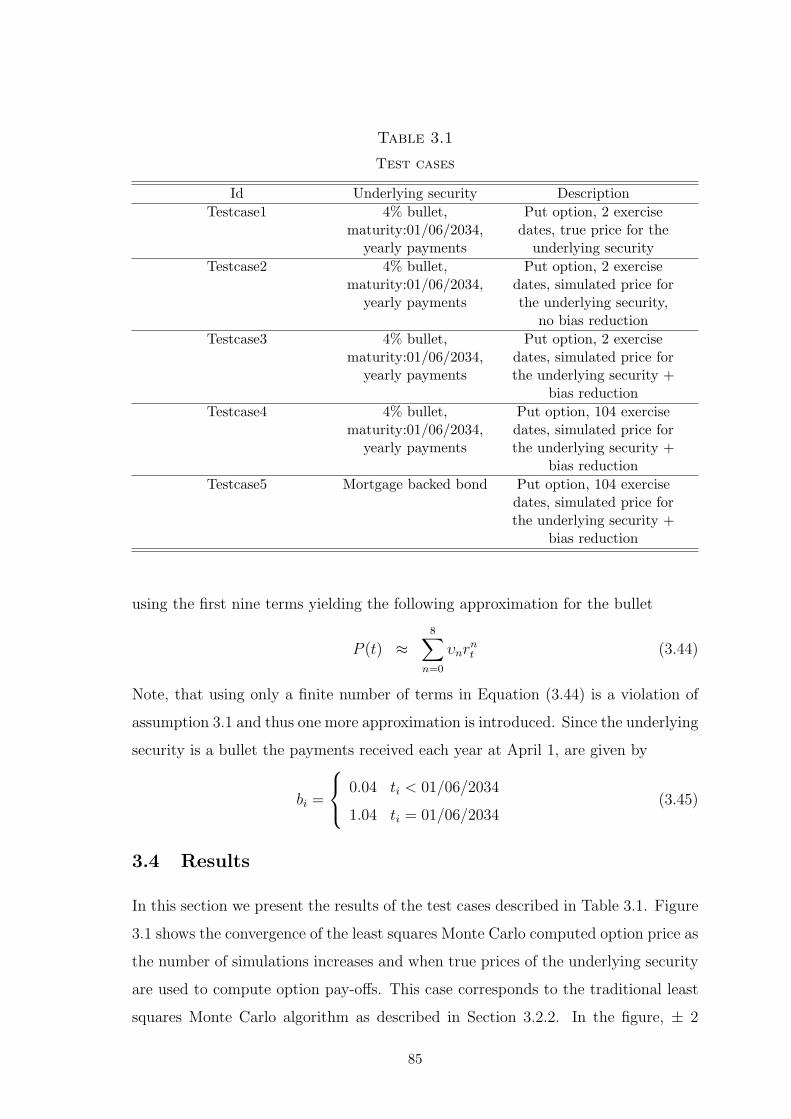
Table 3.1

Test cases

Id Underlying security Description

Testcase1 4% bullet,maturity:01/06/2034,

yearly payments

Put option, 2 exercisedates, true price for the

underlying security


yearly payments

Put option, 2 exercisedates, simulated price forthe underlying security,

no bias reduction


yearly payments

Put option, 2 exercisedates, simulated price forthe underlying security +

bias reduction


yearly payments

Put option, 104 exercisedates, simulated price forthe underlying security +

bias reduction

Testcase5 Mortgage backed bond Put option, 104 exercisedates, simulated price forthe underlying security +

bias reduction

using the first nine terms yielding the following approximation for the bullet

P (t) ≈8∑

n=0

υnrnt (3.44)

Note, that using only a finite number of terms in Equation (3.44) is a violation of

assumption 3.1 and thus one more approximation is introduced. Since the underlying

security is a bullet the payments received each year at April 1, are given by

bi =

0.04 ti < 01/06/2034

1.04 ti = 01/06/2034(3.45)

3.4 Results

In this section we present the results of the test cases described in Table 3.1. Figure

3.1 shows the convergence of the least squares Monte Carlo computed option price as

the number of simulations increases and when true prices of the underlying security

are used to compute option pay-offs. This case corresponds to the traditional least

squares Monte Carlo algorithm as described in Section 3.2.2. In the figure, ± 2

85

Figure 3.1: Testcase1 - Convergence of least squares Monte Carlo.Diamonds represent the average relative pricing error. The upper and lower bar show ± 2 standarddeviation of the pricing error respectively. The dotted lines indicate ±2.5% deviations from the PDEcomputed option price. The sample size is 1000.

standard deviations of the option price estimate are also shown. The dashed lines

indicate ±2.5% deviations from the PDE computed option price. As can be seen, the

least squares Monte Carlo computed option price converges to the PDE computed

option price as the number of simulations increases. Also, not surprisingly, as the

number of simulations increases, the uncertainty of the price estimate decreases. It

is also worth noting that all the price estimates are almost identically to the PDE

computed option price, even for a small number of simulations. This would probably

not be the case if we were to price an option on a more complex underlying than

the option on a bullet we investigate in Figure 3.1.

In Figure 3.2, the convergence of the least squares Monte Carlo computed option

price for Testcase2 is shown. In this test case, true prices of the underlying security

have been replaced with crude Monte Carlo simulated prices when option pay-offs

are computed. No bias reduction are performed. Recall that when option pay-

offs are computed, Algorithm 4 only uses the current path to compute the state

dependent price of the underlying security. Off course this price estimate will be

highly uncertain, since only one single path has been used to simulate the price.

This leads to a high bias in the option pay-off, and we would expect the resulting

least squares Monte Carlo computed option price to be biased high as well. Also,

86


the bias cannot be removed no matter how many simulations we put into computing

the option price. The only way to reduce the bias is to lower the uncertainty of

the crude Monte Carlo estimates of the underlying, which only can be achieved by

increasing the work that is put into generating these prices. In many cases this

is very computationally burdensome and Algorithm 4 is constructed in a way that

makes it impossible to use more than one path in the simulation of the underlying.

When we add bias reduction to Testcase2 we get Testcase3. The convergence

result for this test case is shown in Figure 3.3. For few simulations, the simulated

option price is biased high. But as the number of simulations increase, the bias is

reduced and the option price becomes almost equal to the PDE option price. Recall

that we are only using 9 basis functions in the polynomial approximating the under-

lying bond price, but this does not seem to be of any problem. Another attractive

feature of the algorithm is that both bias reduction and accuracy are improved by

increasing the number of simulations. This is in contrast to Testcase2 in which only

accuracy, but no bias reduction, is improved by increasing the number of simula-

tions. Comparing with Testcase1, in which the true price of the underlying security

was used to compute option pay-offs, the option prices computed in Testcase3 are

very close to the ones computed in Testcase1. Only for 100, 200 and 400 simulations

87


there is a small difference between the option prices in the two test cases. How-

ever, the uncertainty induced by using simulated prices of the underlying security

when computing option pay-offs also turns up in higher uncertainty on the simulated

option price and this higher uncertainty persists even for 204800 simulations.

In Figure 3.4 the price of a Bermudan option with 104 exercise dates has been

simulated. The effect of increasing the number of exercise dates from 2 to 104 is

higher bias and higher standard errors, especially for a low number of simulations.

But as the number of simulations increases, both the bias and the standard errors

are reduced and for approximately 12800 simulations they are at the same low level

as in Testcase3.

Finally, for Testcase5 we have simulated the price of a Bermudan option with

104 exercise dates on a MBS. The results are shown in Figure 3.5. We have not

computed a PDE price for Testcase5, so the values shown are the simulated option

prices. The conclusions are the same as for the previous test cases - both bias and

standard errors are reduced when the number of simulations increase.

88


3.4.1 Estimated Price Relation

In this section we will investigate the estimated price relations of the underlying

security at the exercise dates for Testcase3. These estimated relations are used to

compute option pay-offs and it is therefore crucial that they are good approxima-

tions of the true relation between the price of the underlying security and the state

variables.

In Figure 3.6 the true relation between the price of the coupon bond and the

spot rate is shown at the first exercise date April 6, 2005. The true price relation

can easily be found in the Hull-White model since, in each future state, the entire

yield curve is just an exponential affine function of the spot rate. Thus, the true

price relation fulfills equation 3.42. Figure 3.6 also shows three estimated relations

between the price of the underlying security and the spot rate. These relations

are found by projecting the crude Monte Carlo simulated price estimates of the

underlying security onto powers of the spot rate. I.e. they are approximations of the

expression given by Equation (3.42). The approximations are found using 100, 6400

and 204800 simulations respectively. As can be seen, the approximation becomes

more accurate as the number of simulations increase. For only 100 simulations,

89

Figure 3.5: Testcase5 - Convergence of least squares Monte Carlo.Diamonds represent the average option price. The upper and lower bar shows ± 2 standard deviation ofthe pricing respectively. The sample size is 1000.

the estimated price for high spot rates are completely wrong, whereas it is close

to the true price relation for low and middle ranged spot rates. The reason for

this divergence is that when we only use 100 simulations, there is little or no price

information in the high spot rate region of the state space. The probability of

getting a spot rate, at exercise date 1, above 8% is only 0.11% meaning that on

average only 0.11 out of 100 simulated spot rates will be above 8%. Thus, the

probablity of getting a crude Monte Carlo estimate of the underlying security in this

part of the state space is very low, making the estimated price relation very difficult

to infer. The bias reduction method takes advantages of a diversification effect in

the sense that if one has enough observations, the error term embedded in each

observation can be filtered away. But since the elapsed time from today until the

first exercise date is relatively short, the simulated spot rates are not very dispersed

and will be concentrated around it’s conditional mean at exercise date 1. This can

also be seen in Figure 3.6, namely in regions of the state space where there are many

observations, the estimated price relations are very accurate. Looking at Figure 3.3

we see that the inaccurate estimated price relation of the underlying results in an

inaccurate and biased option price. The reason why the computed option prices are

not that inaccurate in spite of the divergence in the estimated price relation of the

90

Figure 3.6: Testcase3 - Model price-spot rate relation and estimated price-spotrate relation of the underlying coupon bond at exercise date 1. Initial spot rateis 5%

underlying is, that the weight (probability) which these pay-offs get, is relatively low.

Increasing the number of simulations to 6400 and 204800 removes the divergence of

the estimated price relation and with 204800 simulations the estimated price relation

is relatively close to the true price relation for all levels of the spot rate. This can

also be seen in the option prices as a more accurate option price estimate (see Figure

3.3).

Now turn to exercise date 2. In Figure 3.7 the relation between the price of the

underlying and the spot rate is shown for the same models as in Figure 3.6. For

6400 and 204800 simulations the conclusions are the same as for exercise date 1 -

that the estimated price relations are good at approximating the true price relation

over a large range of the state space. For 100 simulations, however, we have a much

better approximation of the true price relation of the underlying. The reason is

the longer time period between today and exercise date 2, which results in more

dispersed spot rates over the state space than for exercise date 1. At exercise date

2, the probability of getting a spot rate above 8% is now 1.34%, more than 10 times

higher than for exercise date 1.

91

Figure 3.7: Testcase3 - Model price-spot rate relation and estimated price-spotrate relation of the underlying coupon bond at exercise date 2. Initial spot rateis 5%

Table 3.2

True coefficients

Coefficient Spot rate Value at exercisedate 1

Value at exercisedate 2

ν0 r0 1.4046 1.3955ν1 r1 -15.6877 -15.4399ν2 r2 102.4994 99.7405ν3 r3 -475.1468 -456.6217ν4 r4 1704.1267 1,616.1862

3.4.2 Estimated Price Coefficients

In Section 3.3.1 we derived an expression for the coefficients to the basis functions

in the Hull-White model for a bullet loan. In this section we investigate the first five

estimated coefficients at exercise date 1 and 2. The true coefficients are computed

by Equation (3.43) and they are summarized in Table 3.2.

In Figure 3.8, the bars show the relative errors on the estimated constant co-

efficient, ν0, as the number of simulations increases. In addition, the standard de-

viations of the relative errors are displayed as lines with values on the right hand

axis. Relative errors and standard deviations of the relative errors are shown for

92

both exercise date 1 and exercise date 2. As can be seen, both the relative error

and the standard deviation of the relative error decreases and approaches zero as

the number of simulations increases. It can also be seen that the relative errors are

lower for exercise date 2 than for exercise date 1, and that the standard deviation

of the relative errors are lower on exercise date 2 than on exercise date 1. The

only major exception for this pattern is the case with 100 simulations, where the

relative error of ν0 is lower on exercise date 1 than on exercise date 2. It is also

worth nothing that, as the number of simulations increases, the differences in terms

of relative errors and standard deviations of the relative errors between exercise date

1 and exercise date 2, vanishes. The reason for this phenomenon is that for a small

number of simulations, the spot rates are more dispersed throughout the state space

on exercise date 2 than they are on exercise date 1. This is illustrated in Figure 3.9

where the solution to the spot rate process in Equation (3.36) has been simulated

on exercise date 1 and exercise date 2 respectively. Note also, that the standard

deviations of the relative errors are very high for a small number of simulations.

The conclusions made for ν0 also apply for the estimated coefficients ν1, ν2,

ν3 and ν4. This is illustrated in Figure 3.10, Figure 3.11, Figure 3.12 and Figure

3.13. The differences is that the level for both the relative error and the standard

deviation of the relative error are much higher, the higher the power of the spot

rate is. This suggests that a large part of variations on prices of the underlying

coupon bond at exercise date 1 and exercise date 2 can be explained by the first

basis functions in the approximation of the price given by (3.44) for this simple

underlying security. This would probably not be the case if the underlying security

were more complex, as would be the case for a mortgage backed bond. However, as

the number of simulations increases, the estimates become more and more accurate,

because the spot rates become more dispersed throughout the state space. Our

results are consistent with the result in (Glasserman & Yu, 2003), saying that the

number of simulations needed grows exponentially in the number of basis functions.

93

Figure 3.8: Testcase3 - Estimated ν0 coefficient.Estimated constant at exercise date 1 and 2. The bars show the average relative error and are relatedto the left axis. The lines show the standard deviation of the estimate and are related to the right axis.The sample size is 1000.

3.5 Conclusion

In this paper we develop an algorithm aimed at simulating Bermudan option prices

written on securities that must also be priced by simulations. The method extends

the algorithm developed in (F. Longstaff & Schwartz, 2001) by applying the bias

reduction technique from (Huge & Rom-Poulsen, 2004) to reduce the bias in the

option price induced by using noisy price estimates of the underlying security in the

dynamic programming recursion. We show that if the price of the underlying secu-

rity belongs to a space spanned by some basis functions, the result of the algorithm

approaches the solution to the programming problem in (F. Longstaff & Schwartz,

2001). (Clemente et al., 2002) prove that this solution approaches the true option

price as the number of basis functions and paths approaches infinity. However,

generally the spanning assumption is not fulfilled, and the bias reduction thus in-

troduces an additional approximation besides those introduced using the algorithm

in (F. Longstaff & Schwartz, 2001).

We demonstrate, using simple test cases, that the algorithm is capable of com-

puting Bermuda option prices that are very close to the option prices computed

using a PDE approach.

94

Figure 3.9: Simulated Hull-White spot rate distributionSimulated spot rate distribution at exercise date 1 and exercise date 2 respectively for the parametervalues in Testcase3. 30.000 simulations have been used.

The estimated coefficients to the basis functions seem to approach their true val-

ues, especially for the coefficients multiplying low powers of the spot rate. However,

for a small number of simulations, the standard deviation of the estimated coefficient

is extremely high. Many simulations are needed in order to get accurate coefficient

estimates. This is in line with the findings in (Glasserman & Yu, 2003).

Using many simulations yields relatively accurate coefficient estimates and this,

in turn, results in relatively good approximations of the relations between the price

of the underlying and the spot rate. However, for a small number of simulations

and short term exercise dates, the relation between the price of the underlying and

the spot rate is only accurate in non-extreme regions of the state space. Thus, one

must be sure to use a sufficient number of paths when simulating Bermudan option

prices with a strike corresponding to extreme values of the state variables.

95

Figure 3.10: Testcase3 - Estimated ν1 coefficient.Estimated ν1 at exercise date 1 and 2. The bars show the average relative error and are related to theleft axis. The lines show the standard deviation of the estimate and are related to the right axis. Thesample size is 1000.


96



97

3.6 Appendix A: Proofs


We want to show that the solution to the dynamic programming problem in Section

3.2.3 approaches the solution to the problem in Section 3.2.2 when the approximation

in Equation (3.30) is used. In the following, we emphasise the dependence of the

number of paths U used in the simulation of the state space and thus used in

Equation (3.30) to estimate the coefficients in the least squares price estimate. By

Assumptions 3.1 and 3.2, the price of the underlying security fulfils PLSi (Xi;U) →

Pi(Xi) ∀ i as U increases. Thus we have ∀ i

hLSi (Xi;U) → hi(Xi) as U → ∞

By definition CLSL (XL;U) = CL(XL) = 0 and V LS

L (XL;U) = hLSL (XL;U) → hL(XL) =

VL(XL) as U → ∞. The proof now goes by induction. Assume that V LSj (Xj;U) →

Vj(Xj) as U → ∞, for j = i+ 1, . . . , L. If we can prove that CLSi (Xi;U) → Ci(Xi)

as U → ∞, then we have V LSi (Xi;U) → Vi(Xi) as U → ∞ and we are done. Now

from (3.23)

CLSi (Xi;U) =

R∑

r=1

ζLSir (U)ψir(Xi)

where

ζLSi (U) = (EQ

i [ψi(Xi)ψi(Xi)T])−1E

Qi [ψi(Xi)V

LSi+1(Xi+1;U)]

If

EQi [ψi(Xi)V

LSi+1(Xi+1;U)] → E

Qi [ψi(Xi)Vi+1(Xi+1)] as U → ∞ (3.46)

then ζLSi (U) → ζi as U → ∞, which implies that CLS

i (Xi;U) → Ci(Xi) as U → ∞Since ψi(Xi)V

LSi+1(Xi+1;U) defines a sequence of stochastic variables as U in-

creases, a sufficient condition for (3.46) is (3.32) and (3.33).

98

Chapter 4

Semi-Analytic MBS Pricing1

1This Essay is forthcoming in The Journal of Real Estate Finance and Economics. I am grateful to

Lars Peter Lilleøre, Allan Mortensen and Carsten Sørensen for useful discussions and comments. All errors

are of course my own.

99

Abstract

This paper presents a multi-factor valuation model for callable mortgage backed

securities (MBS). The model gives semi-analytic solutions for the value of MBS. By

modelling the size of the remaining debt, also known as the pool size, we show that

the value of a single MBS payment due at time tn can be found by computing two

expectations of the pool size at tn−1 and tn, respectively. To obtain semi-analytic

solutions, we specify the pool size in such a way that these expectations can be

computed by transform methods. The expectations are taken of two simple pay-offs,

but instead of using the spot rate for discounting, a prepayment-adjusted discounting

rate must be used. By combining the affine and quadratic pricing frameworks,

flexible and sophisticated prepayment functions can be specified. The result is a

MBS pricing model that is able to generate negative convexity as interest rates fall

and still be close to the non-callable counterpart as interest rates rise. The valuation

model is potentially useful in managing large MBS portfolios and in pricing options

on MBS.

100

4.1 Introduction

In this paper a semi-analytic model for pricing fixed-rate callable mortgage backed

securities (MBS) is presented. The model is based on ideas from credit risk modelling

and belongs to the class of intensity-based models. At almost no computational cost

the model can handle multiple state variables. Usually, MBS are priced with lattice

methods, finite difference or Monte Carlo simulations, which is the only alternative

if the dimension of the state space is high. The presented model thus offers an

attractive alternative if computational speed is an important factor.

A callable mortgage backed security is a pass-through giving borrowers, at any

point in time, the possibility to cancel their loans by paying back the outstanding

loan balance at par. From the investor’s perspective, a MBS is a fixed rate bond

plus a sold American call option on the remaining scheduled cash flow. In principle,

prices of MBS can be computed by valuing the embedded American style option

using standard option pricing theory. In its purest form, this procedure implicitly

assumes that all debt holders prepay the first time it is economically profitable, a

decision that is made endogenously within the model. However, such a model will

produce MBS prices that only exceed par with the cost of prepaying, usually a few

percent of the debt size. This is not consistent with observations in the market where

some mortgage holders prepay as soon as it is profitable and others do not prepay at

all, leading to MBS prices that far exceed par. To handle this heterogeneity among

borrowers, different types of models have been proposed. One class of models uses

an econometric model to explain prepayments by some exogenous variables that are

assumed to determine the mortgagor’s prepayment decision. The most important

explanatory variable in these models is the gain from refinancing. The model is

then estimated by fitting it to observed prepayment data, and the heterogeneity

among borrowers becomes a function of observed variables. Another line of research

holds on to the rational hypothesis in option pricing theory and let differences in

prepayment costs drive the heterogeneity among borrowers. Typically, such models

assume that mortgage holders minimize their lifetime mortgage costs, which include

both economical and non-economical costs. Examples of the first class of models are

(Schwartz & Torous, 1989) and (Jakobsen, 1992) and examples of the second class

101

of models are (Stanton, 1995), (Kau, C., Muller III, & Epperson, 1995), (Yongheng,

Quigley, & Van Order, 2000). (F. A. Longstaff, 2002) also belongs to the second

class of models, and he extends the concept of costs to include borrower credit

worthiness (see (Kau & Keenan, 1995) for an overview of the option approach for

MBS pricing). In recent years, models that use elements from credit risk modelling

to price MBS have emerged. This is for example the case in (Collin-Dufresne &

Harding, 1999), (Kariya & Kobayashi, 2000), (Nakamura, 2001) and (Kau, Keenan,

& Smurov, 2004).

In this paper an intensity-based model for pricing callable MBS is constructed.

By modelling the pool size2 instead of the conditional prepayment rate3 (CPR) as

is usual, we are able to derive a semi-analytic formula for the price of a callable

MBS. The trick is to specify the pool size in such a way that it has a form that looks

similar to the pay-offs that can be valued semi-analytically in the pricing frameworks

of (Duffie, Pan, & Singleton, 2000) and (Leippold & Wu, 2002). From the pool sizes,

an expression for the instantaneous CPR is derived and it is eventually this function

that must be estimated. In this respect our model belongs to the first class of models

described above. Using this specification, the value of a single MBS payment can be

computed by valuing two simple pay-offs that only depend on the state variables at

payment time. However, instead of discounting the pay-offs with the spot rate, they

must be discounted by a prepayment-adjusted rate defined by the instantaneous

CPR function. The advantage of this approach is that the values of these pay-offs

are known in semi-analytic form. In the (Duffie et al., 2000) pricing framework, they

are given as exponential affine functions of the state variables, and in the (Leippold

& Wu, 2002) pricing framework they are given as quadratic exponential functions

of the state variables. The coefficients on the state variables (and squared state

variables) are in both cases deterministic functions of time, which in both the affine

and quadratic pricing framework are found by solving a set of coupled ordinary

differential equations (ODE). This, in turn, yields semi-analytical pricing formulas

for the MBS price. Moreover, this ODE system only has to be solved once in order to

value all payments from a particular MBS. The presented model can handle multiple

2The pool size measures how many loans are left in the pool of mortgage loans.3The conditional prepayment rate gives the proportion of the pool size that prepays during a given

period.

102

state variables allowing for realistic yield curve dynamics and a flexible specification

of the prepayment model. We do not, however, model any burn out effects. A simple

way to introduce burn out is to divide the MBS pool into sub-pools, each with its

own prepayment model.

In this paper, a two factor affine term structure model (ATSM) is employed as

the underlying interest rate model. More precisely, the two-factor shifted Gaussian

model from (Brigo & Mercurio, 2001) is used. (Litterman & Scheinkman, 1991)

show that yield curve dynamics are best described by using two or three state vari-

ables. Another reason for using multiple state variables is that correlation between

rates of different maturities are decoupled allowing the prepayment model to depend

on both short and long rates. The model fits into the (Duffie et al., 2000) pricing

framework and provides closed form solutions for a wide range of securities. How-

ever, the pay-offs that can be priced must be affine functions of the state variables.

A good model for pricing MBS is a model in which CPR speeds up as interest rates

fall. In (Schwartz & Torous, 1989) this is done by including cubic terms of the

refinancing incentive. In our model, however, quadratic terms are used to acceler-

ate prepayments for sufficiently low interest rates. The reason for using quadratic

terms is that the quadratic pricing framework can then be applied. Quadratic terms

structure models (QTSM) like ATSM, yield closed form solutions for many interest

rate products. The difference between an ATSM and a QTSM is that in the for-

mer, the spot rate is given as an affine function of the state variables whereas in

the latter, the spot rate is a quadratic function of the state variables. From (Dai

& Singleton, 2000) we know that in ATSM, Gaussian and square root processes

can be mixed. In QSTM, however, only Gaussian processes are allowed. The main

reason that we have chosen the two-factor shifted Gaussian term structure model is

that it also fits into the quadratic pricing framework. Since spot rates are affine in

the state variables, we are now allowed to build prepayment functions that depend

on quadratic terms of the spot rate and still remain within the quadratic pricing

framework. Put another way, we mix the two pricing frameworks by working in the

area where ATSM and QTSM coincide, to get a more sophisticated description of

prepayments.4

4See (Duffie & Kan, 1996), (Dai & Singleton, 2000) and (Duffie et al., 2000) for papers on ATSM and

103

The paper by (Collin-Dufresne & Harding, 1999) is the one closest to the study

in this article. Using an affine term structure model5, they derive semi-analytic

pricing formulas for MBS. However, they are restricted to one-factor models. The

specification of the instantaneous CPR is, like in our model, restricted to a specific

form in order for their argument to work. We extend the work done in (Collin-

Dufresne & Harding, 1999) by allowing for multiple state variables, which allows for

a more sophisticated specification of the prepayment model. Since this model is so

closely related to our work we will take a closer look at this model and show how it

can be cast into the more general pricing framework of (Duffie et al., 2000), which

also allows for jumps in the state variables. (Nakamura, 2001) also obtains semi-

analytic MBS pricing formulas by modelling the individual loan’s exit time from the

pool of mortgage loans.

We only consider MBS that are backed by the issuing institution and thus we

treat them as default-free. Some papers in the literature also model prepayments

resulting from mortgagors’ defaulting, which rationally happens when the value of

the remaining mortgage payments exceeds the value of the property. In Denmark,

however, some MBS pools are backed by the other mortgage holders in the pool and

other MBS pools are backed by the issuing institution. This makes the need for

modelling the default option less important for Danish MBS and we do not consider

it in this study. Papers that include the default option are (Kau et al., 1995), (Kau

& Keenan, 1995), (Yongheng et al., 2000), (Nakamura, 2001) and (Kau et al., 2004).

Besides providing fast computation of MBS prices and price sensitivities, the

model can be used to construct efficient pricing routines for pricing options on

callable MBS and prepayment dependent pay-offs. The price of a European op-

tion on a MBS for example, can be computed by simulating the state variables from

today until option expiration, where the price of the underlying MBS is known in

semi-analytic form, providing fast computation of the option pay-off.6 Alternatively,

(Jamshidian, 1996), (Ahn, Dittmar, & Gallant, 2002), (Leippold & Wu, 2002), (Cheng & Scaillet, 2004)

and (Chen, Filipovic, & Poor, 2004) for papers on quadratic term structures.5Their reported results are based on a Vasicek one-factor model, but their result carries over to all affine

one-factor models.6Also, since Gaussian state variables are used, the joint distribution of the state variables is known,

allowing for single-step simulation when no pool factor is present.

104

a new pricing routine would have to be initiated to compute the state dependent

MBS price at option expiration as done in (Huge & Rom-Poulsen, 2004). A pre-

payment cap is a cap on prepayments made at a particular payment date. Since

the pool size is a known function of the state variables, the value of a prepayment

cap can easily be computed by a Fourier inversion of the discounted cap pay-off.

The inversion must typically be done numerically, but since it implies solving a

one-dimensional integral, efficient numerical routines exist.

The paper is organized as follows; in Section 4.2 the pool size is defined and

we show how it is related to CPR. Furthermore, we show how to value a single

mortgage payment by decomposing the mortgage into two terms that must be valued

separately. This result is quite general and does not depend on any term structure

model. In Section 4.3 both the affine and the quadratic pricing frameworks are

introduced. Section 4.4 shows how the (Collin-Dufresne & Harding, 1999) model

can be cast into the (Duffie et al., 2000) pricing framework. In Section 4.5, the

specific two-factor intensity-based model for pricing MBS is introduced. First we

present the shifted Gaussian interest rate model and then we present the prepayment

model. Section 4.6 contains results from the model. Finally, Section 4.7 concludes

on the paper.

4.2 Pool Size, CPR and Mortgage Payments

In each period, [ti−1, ti], a percentage of the mortgage holders in the pool decide

to prepay their loans. This percentage is called CPR(ti−1, ti) and it depends on

the state of the economy through the vector of state variables Xi.7 The remaining

amount of loans left in the pool after n periods is called the pool size and is denoted

by Qn. The relation between CPR and pool size is

Qn ≡n∏

j=1

(1 − CPR(tj−1, tj)) (4.1)

and in terms of the pool size, the CPR for the period (ti−1, ti] is given by

CPR(ti−1, ti) =Qi−1 −Qi

Qi−1

(4.2)

7For readability the following notation will be used Xi = Xti.

105

Relation (4.2) states that the CPR is the amount of terminated loans in a period

relative to the remaining loans left in the pool at the beginning of the period.

The pricing models to be used are formulated in continuous time and thus we

define the instantaneous CPR as

f(Xt) = lim∆→0

(

CPR(t, t+ ∆)

∆

)

=1

Qt

lim∆→0

Qt −Qt+∆

∆

= −dQt/dt

Qt

= − d

dtlnQt

which yields the following relation between the instantaneous CPR and the pool size

Qt = e−∫ t

0 f(Xu) du (4.3)

Ito’s lemma gives

dQt = −f(Xt)Qtdt ,Qs = qs (4.4)

which says that over time, the pool size depreciates continuously at the rate f(Xt).

Also, by Equation (4.2), CPR(ti−1, ti) = 1 −Qi/Qi−1, which yields

f(Xi) ≈− ln (1 − CPR(ti−1, ti))

ti − ti−1

(4.5)

over small intervals.

In this paper, instead of modelling CPR(tj−1, tj), the primary object to be mod-

elled is Qj, which basically means that we are modelling the instantaneous CPR,

f(Xt). However, f(Xt) cannot be chosen arbitrary since the following properties

must be fulfilled

• Q0 = 1

• Qt ∈ [0, 1] ∀ t

• Qt must be a non-increasing function of time

Furthermore, to obtain realistic prepayment functions, one would usually require

that

• f(Xt) must be negatively correlated with interest rates

106

The first property states that the pool size at the time of MBS origination is equal to

1 and it is satisfied by construction as stated in relation (4.3). The second property

states that the pool size must belong to the interval [0, 1]. The third property states

that the pool size cannot rise, which basically is the same as requiring that f(Xt)

is non-negative. The last property implies that CPR is negatively correlated with

interest rates, which is a requirement because we want prepayments to rise when

interest rates fall, and prepayments to fall when interest rates rise. The property

is easily achieved, since the factors explaining prepayments are the same as the

factors explaining interest rates. Alternatively, if the instantaneous CPR, f(Xt),

was modelled by a separate state variable process, this process must be negatively

correlated with the state variables driving interest rates.8

The general expression for a single MBS payment due at time tn is

hn =∏n−1

j=1 (1 − CPR(tj−1, tj))

(CPR(tn−1, tn)(Hn +Rn) + (1 − CPR(tn−1, tn))(On +Rn))(4.6)

where Hn is the remaining debt as scheduled if no prepayments occur before any

redemption payment is made, Rn is the scheduled interest payment, and On is the

scheduled redemption payment. The product term scales the pool size according

to prepayments up to time tn−1. At tn a fraction of the mortgagors prepay their

loans, this fraction is given by CPR(tn−1, tn). Borrowers who prepay must return

the remaining debt balance given by Hn and interest for the period given by Rn.

Borrowers who do not prepay make a scheduled redemption payment, On, and must

also pay interest for the period.9

Insert into Equation (4.6) the expression for the pool size Equation (4.1) and the

expression for the CPR Equation (4.2) to get

hn = Qn−1

((

Qn−1 −Qn

Qn−1

)

(Hn +Rn) +Qn

Qn−1

(On +Rn)

)

= Qn−1 (Hn +Rn) −Qn (Hn −On) (4.7)

Note that On, Rn, and Hn are known when the MBS is issued.

8This is another reason to use a QTSM rather than a ATSM when pricing MBS. Negative correlation

between state variables and positiveness of the state variables is not possible in ATSM, see (Dai & Singleton,

2000) page 1956.9Setting CPR(tj−1, tj) = 0 ∀j yields the cash flow from a non-callable bond.

107

Thus, by formulating the MBS payment in terms of the pool size as in Equation

(4.7) instead of the CPR as in Equation (4.6), the nasty term∏n

j=1(1−CPR(tj−1, tj))

disappears. Having the MBS payment due at time tn expressed in terms of functions

of the pool size at time tn−1 and tn greatly simplifies the pricing of MBS, as will

become clear in the following sections.

We are now ready to compute the value of a single MBS payment. The time t

value of a mortgage payment due at time tn is equal to

V (t, hn) = EQt

[

e−∫ tn

tr(Xu) duhn

]

= (Hn +Rn)EQt

[

e−∫ tn

tr(Xu) duQn−1

]

− (Hn −On)EQt

[

e−∫ tn

tr(Xu) duQn

]

= (Hn +Rn)EQt

[

e−∫ tn−1

t r(Xu) duQn−1EQtn−1

[

e−∫ tn

tn−1r(Xu) du

]]

− (Hn −On)EQt

[

e−∫ tn

tr(Xu) duQn

]

= (Hn +Rn)EQt

[

e−∫ tn−1

t r(Xu) duQn−1P (tn−1, tn)]

− (Hn −On)EQt

[

e−∫ tn

tr(Xu) duQn

]

(4.8)

where the expectation is taken under the risk-neutral probability measure and where

P (tn−1, tn) is the time tn−1 price of a zero coupon bond with maturity at time tn.

Inserting the expression for Qn yields

V (t, hn) = (Hn +Rn)QtEQt

[

e−∫ tn−1

t (r(Xu)+f(Xu)) duP (tn−1, tn)]

− (Hn −On)QtEQt

[

e−∫ tn

t(r(Xu)+f(Xu)) du

]

(4.9)

The quantity Qt = e−∫ t

0 f(Xu) du is the time t pool factor, i.e. the remaining pool size

at time t. If we want the prepayment function to be dependent on the pool size, this

is the object that should enter into the prepayment function. Typically the current

pool factor is approximated by the total current debt size relative to the initial debt

size.

From the expression for the value of a single MBS payment, the MBS value

is found by adding the values of all its payments. Note that the price computed

by Equation (4.9) is the price for a pool size of Qt = e−∫ t

0 f(Xu) du. Market prices,

108

however, are typically quoted for a pool size of 100. Thus, when normalised to a

pool size of 1 the term e−∫ t

0 f(Xu) du in (4.9) disappears.

The complicated task of finding the value of the expression in Equation (4.6) has

now been reduced to that of computing the time t value of the pay-offs P (tn−1, tn)

and 1. However, instead of using the spot rate, r(Xt), for discounting, we must

use a prepayment-adjusted rate equal to r(Xt) + f(Xt). In other words, payments

from callable MBS are discounted at a higher rate than payments from non-callable

securities. In this respect, the formulation given here is similar to an intensity-based

model used for pricing securities that are subject to credit risk. In intensity-based

models, payments from bonds with credit risk are discounted by a spot rate plus a

stochastic intensity representing the default risk of the bond in question. See e.g.

(Lando, 2004) for a description of intensity-based credit risk models.

4.3 Computational Framework

In this section a short description of the affine and the quadratic pricing frameworks

is given. In ATSM the spot rate is an affine function of the state variables and in

QTSM the spot rate is a quadratic function of the state variables. Both frameworks

give closed form pricing solutions for a wide range of pay-offs. The restriction is

that the pay-offs can be written as an exponential affine or an exponential quadratic

form of the state variables. Both models allow for jumps in the state processes, but

this is not used in this paper.

A completed filtered probability space(

Ω,F , FtTt=0 ,Q

)

is taken as given. The

filtration is generated by the relevant price processes in the economy. We assume

the existence of a risk-neutral martingale measure, Q, under which all expectations

are taken. Assume that the uncertainty of the economy is described by a vector of

state variables10

dXt = µ(t,Xt)dt+ σ(t,Xt)dWt (4.10)

where µ(t,X) is a n×1 vector defining the drift, σ(t,X) is a n×n matrix defining the

diffusion of the process, and Wt is a n× 1 vector of independent Brownian motions

10To include jumps in ATSM see (Duffie et al., 2000). To include jumps in QTSM see (Cheng & Scaillet,

2004).

109

under Q.

4.3.1 The Duffie, Pan, and Singleton (2000) Framework

The affine set-up puts an affine structure on µ, σσT and the spot rate, r(Xt), as

stated in the following

µ(t,Xt) = K0 +K1Xt, for K0 ∈ Rn, K1 ∈ Rn×n

(σ(t,Xt)σ(t,Xt)T)ij = (H0)ij + (H1)ij ·Xt for H0 ∈ Rn×n, H1 ∈ Rn×n×n

r(Xt) = ω0 + ω1 ·Xt for ω0 ∈ R, ω1 ∈ Rn

The transform defined by

ψ(u,Xt, t, T ) = EQt

[

exp

(

−∫ T

t

r(Xs) ds

)

eu·XT

]

(4.11)

is known in closed form with solution

ψ(u,Xt, t, T ) = eα(t,T )+β(t,T )·Xt (4.12)

where α(t, T ) and β(t, T ) are solutions to the following ODEs

β(t) = ω1 −KT

1β(t) − 12β(t)TH1β(t), β(T ) = u

α(t) = ω0 −K0 · β(t) − 12β(t)TH0β(t), α(T ) = 0

(4.13)

The transform in (4.11) is in fact the price at time t of a pay-off eu·XT at time

T and many pay-offs can be cast into this form allowing for semi-analytic pricing.

For example, the price of a zero coupon bond is obtained by solving the ODEs in

(4.13) with u = 0. If we allow for complex numbers, and price a security with time

T pay-off equal to eiuXt , where i =√−1, the transform in (4.11) actually gives

us the discounted characteristic function for the stochastic variable XT , which is

the foundation for using Fourier transforms in option pricing. See also (Bakshi &

Madan, 2000) for properties of this transform.

4.3.2 Quadratic Interest Rate Modelling

In quadratic term structure models the spot rate is a quadratic function of the

state variables. This framework is a little more restrictive when specifying the state

110

variables in that only Gaussian processes are allowed.

µ(t,Xt) = K0 +K1Xt, for K0 ∈ Rn, K1 ∈ Rn×n

(σ(t,Xt)σ(t,Xt)T)ij = ΣΣT for Σ ∈ Rn×n

r(Xt) = cr + bT

rXt +XT

t ArXt for cr ∈ R, br ∈ Rn, Ar ∈ Rn×n

Positive spot interest rates are guaranteed by assuming Ar to be positive semidefinite

and having cr − 14bT

rA−1r br ≥ 0.11 Note that in quadratic term structure models, the

volatility is not allowed to depend on the state process vector.

The transform defined by

φ(u,Xt, t, T ) = EQt

[

exp

(

−∫ T

t

r(Xs) ds

)

euTXT +XT

TvXT

]

(4.14)

with u ∈ Rn and v ∈ Rn×n is known in closed form with solution

ψ(u,Xt, t, T ) = eα(t,T )+β(t,T )TXt+XTt γ(t,T )Xt (4.15)

where α(t, T ), β(t, T ) and γ(t, T ) are solutions to the following ODEs

γ(t) = Ar − 2KT

1γ(t) − 2γ(t)TΣΣTγ(t), γ(T ) = v

β(t) = br −KT

1β(t) − 2γ(t)TK0 − 2γ(t)TΣΣTβ(t), β(T ) = u

α(t) = cr −KT

0β(t) − 12β(t)TΣΣTβ(t) − tr (ΣΣTγ(t)) , α(T ) = 0

(4.16)

In Appendix 4.8, the ODEs are derived for the quadratic case. The ODEs in the

affine case can be derived in the same way by setting the quadratic term equal to

zero.

4.4 The Collin-Dufresne and Harding (1999) Model

Since the (Collin-Dufresne & Harding, 1999) model is similar to our model, this

section takes a closer look at it and shows how to solve the model with the techniques

used in this paper. In the original (Collin-Dufresne & Harding, 1999) paper only one-

factor ATSM are allowed12, but this section demonstrates that their model in fact

can cope with multiple factors by casting it into the (Duffie et al., 2000) affine pricing

11To see this, differentiate r(Xt) with respect to Xt to find the Xt at which r(Xt) attains its minimum.

Then insert this Xt into r(Xt) to find the restriction.12As stated in (Collin-Dufresne & Harding, 1999) page 134; ”we are limited to a single state variable,

the interest rate.”

111

framework. In the (Collin-Dufresne & Harding, 1999) model the instantaneous CPR

is defined as

f(Xt) = a0 + a1 ln

(

P (0, T )

P (t, T )

)

= a0 + a1(α(0, T ) + β(0, T )r0) − a1(α(t, T ) + β(t, T )rt) (4.17)

where P (t, T ) is the time t price of a zero coupon bond maturing at time T and T

is the MBS maturity date. The mortgage bond is issued at time 0 and is priced at

time t. The fraction ln(P (0, T )/P (t, T )) is a measure for the refinancing incentive,

thus a1 ≤ 0. The instantaneous CPR is linear in the spot rate and there is nothing

to accelerate prepayments when interest rates becomes sufficiently low. This is a

drawback of the model. Note also that it is possible for f(Xt) to become negative

for some choices of a0 and a1.

In this model, no bond specific variables enter the CPR function. This means

that two different mortgage pools will have the same model price if they were issued

at the same date and have the same maturity. Thus, the model implicitly assumes

homogeneous mortgage holders over different pools. It is easy, however, to extend

the model to take into account, for example, the coupon rate and time-to-maturity.

For an example of how this could be incorporated into the model see Section 4.5.2.

Using a Vasicek interest rate model, the price of a mortgage bond with a continu-

ous payout is computed by solving ODEs and numerical integration. The dynamics

of the spot rate is given by

drt = κ (θ − rt) dt+ σdWt (4.18)

where Wt is a one-dimensional standard Brownian motion. The Vasicek model

belongs to the class of affine term structure models and thus the framework from

(Duffie et al., 2000) can be applied.

Prices of zero coupon bonds are obtained by taking u = 0 in (4.11), which yields

112

the well-know solutions to the ODEs in the Vasicek model13

P (t, T ) = eα(t,T )+β(t,T )rt

β(t, T ) = 1κ

(

e−κ(T−t) − 1)

α(t, T ) =(

σ2

2κ2 − θ)

(β(t, T ) + (T − t)) − σ2

4κβ(t, T )2

(4.19)

It is straightforward to extend this set-up to cope with deterministic coefficients

in r(Xt) instead of constant coefficients. This is necessary since the discounting

term in Equation (4.20) below has deterministic ω1(t, T ) = (1 − a1β(t, T )). The

extension is carried out simply by replacing the constant ω1 in Equation (4.13) with

its deterministic counterpart.

Using the form for prices of zero coupon bonds from (4.19) and using the equa-

tions (4.17) and (4.9) the value of a mortgage payment can be written

V (t, bn) = (Hn +Rn)eα(tn−1,tn)C(t, tn−1)

EQt

[

e−∫ tn−1

t (1−a1β(u,T ))ru dueβ(tn−1,tn)rtn−1

]

− (Hn −On)C(t, tn)EQt

[

e−∫ tn

t(1−a1β(u,T ))ru du

]

(4.20)

where

C(t, tn) =

exp

(

a1

∫ tn

t

α(u, T ) du− (tn − t)(a0 + a1(α(0, T ) + β(0, T )r0))

)

(4.21)

Using footnote 13 we immediately have

∫ tn

t

α(u, T ) du =

(

σ2

2κ2− θ

)[(

T − 1

2tn

)

tn −(

T − 1

2t

)

t

]

+

(

3σ2

4κ3− θ

κ

)

[β(tn, t) − β(t, T ) − (tn − t)]

+σ2

8κ2

(

β(t, T )2 − β(tn, T )2)

(4.22)

Each of the two expectations in (4.20) can be computed using the (Duffie et al.,

2000) framework from Section 4.3.1. Their solutions have the form given in (4.12)

where α(t, T ) and β(t, T ) solves the ODEs (4.55) in Appendix 4.8 with boundary

conditions β(tn−1, tn) and 0 respectively and ω1 = (1 − a1β(t, T )).

13For later use we note that∫ tn

tβ(u, T ) du = 1

κ(β(tn, T ) − β(t, T ) − (tn − t)) and

∫ tn

tβ(u, T )2 du =

1κ2 (β(t, T ) − β(tn, T ) + (tn − t)) − 1

2κ(β(t, T )2 − β(tn, T )2)

113

4.5 An Intensity-Based Model for MBS Pricing

4.5.1 The Stochastic Interest Rate Model

In this section the intensity-based MBS pricing model is put forward. The general

result from Section 4.2 is used to construct a specific model for valuing MBS semi-

analytically. First, however, the interest rate model is presented, followed by the

prepayment model. Since we want prepayments to depend on interest rates in a

quadratic way, the term structure model is restricted to have a Gaussian specifica-

tion. Thus, the relatively flexible G2++ model from (Brigo & Mercurio, 2001) is

applied. The G2++ model is a two factor short rate model where the spot rate is

given by

r(Xt) = ϕ(t) + bT

rXt , bT

r = [1 1] (4.23)

with r(X0) = r0 and where the state variables have the following Q-dynamics

dXt = −

a 0

0 b

Xtdt+

σ 0

ηρ η√

1 − ρ2

dWt , X0 =

0

0

(4.24)

where dWt is a two dimensional vector of independent Brownian motions. Correla-

tion between the two factors is modelled by having a non-zero entry in Σ21 = ηρ.

The reason for this is that the formulations in both (Duffie et al., 2000) and (Leip-

pold & Wu, 2002) assume independent Brownian motions. In contrast, (Brigo &

Mercurio, 2001) work with correlated Brownian motion, but of course, the two for-

mulations lead to identical pricing formulas. r0, a, b, σ, η are positive constants and

−1 ≤ ρ ≤ 1 is the correlation. ϕ(t) is a deterministic function with ϕ0 = r0 used to

match the initial yield curve.

ϕ(T ) = fM(0, T ) +σ2

2a2

(

1 − e−aT)2

+η2

2b2(

1 − e−bT)2

+ ρση

ab

(

1 − e−aT) (

1 − e−bT)

(4.25)

fM(0, T ) is the market instantaneous forward rate at time 0 for maturity T defined

by

fM(0, T ) = −∂ lnPM(0, T )

∂T(4.26)

114

and PM(0, T ) is the price of a zero coupon bond with maturity T currently observed

in the market.

The model yields closed form solutions for a wide range of interest rate products.

Especially, there exist closed form solutions for zero coupon bonds, European options

on zero coupon bonds, interest rate caplets and European swaptions.

Defining the functions

β1(t, T ) = 1a

(

e−a(T−t) − 1)

β2(t, T ) = 1b

(

e−b(T−t) − 1)

(4.27)

allows us to write the yield on a zero coupon bond as

y(Xt, T ) =1

T − t

(∫ T

t

ϕ(u)du− β1(t, T )X1,t − β2(t, T )X2,t −1

2V (t, T )

)

(4.28)

where

V (t, T ) =σ2

a2

[

T − t+2

ae−a(T−t) − 1

2ae−2a(T−t) − 3

2a

]

+η2

b2

[

T − t+2

be−b(T−t) − 1

2be−2b(T−t) − 3

2b

]

(4.29)

+2ρση

ab

[

T − t+ β1(t, T ) + β2(t, T ) − 1

a+ b

(

e−(a+b)(T−t) − 1)

]

and

exp

(

−∫ T

t

ϕ(u)du

)

=PM(0, T )

PM(0, t)exp

(

−1

2[V (0, T ) − V (0, t)]

)

(4.30)

The two processes X1,t and X2,t drive the spot rate and they are correlated

through the diffusion term for X2,t. In contrast to one-factor models, yields of dif-

ferent maturities are not perfectly correlated in multi-factor term structure models,

why it makes sense to build a prepayment function that depends on both the short

and long rate. This is an attractive feature since a mortgagor (at least in Denmark)

faces both refinancing alternatives in the short end of the yield curve in the form

of adjustable-rate mortgage loans, and refinancing alternatives in the long end of

the yield curve in the form of fixed-rate callable loans. In the quadratic pricing

framework the pay-offs that can be priced are allowed to be quadratic in the state

variables. This means that if we let the spot rate be an affine function of the state

variables, the prepayment function can be quadratic in the spot rate. However,

115

Table 4.1

Parameters in the Shifted Gaussian Two-Factor Model

Parameter Value

a 0.1467b 0.3037σ 0.02742η 0.03457ρ -0.8330

Notes: Parameters in the G2++ model taken from (Andersen & Andreasen, 2001).

since only Gaussian processes are allowed, the positiveness of the spot rate cannot

be guaranteed.

We only consider prepayments that are functions of X1 and X2. However, it

would be straightforward to introduce a third source of uncertainty by introduc-

ing a state variable representing non-interest driven prepayments. This could be

relevant since prepayments can change dramatically when new refinancing oppor-

tunities comes to the market. This also suggests that including jumps into such a

state process could be a good idea.14

For our numerical illustrations we have taken the parameter values of the G2++

term structure model from (Andersen & Andreasen, 2001). The values are shown

in Table 4.1. ϕ(t) is then chosen to match the Danish swap curve as of January 3,

2005. The yield curve is shown in Figure 4.1.

4.5.2 The Prepayment Model

In the quadratic pricing framework the CPR function is allowed to have the following

form

f(Xt) = c+ bTXt +XT

t AXt (4.31)

where A is a n× n matrix, b is a vector of size n and c is a scalar. It is possible to

ensure positivity of f(Xt) by A being positive semidefinite and having c− 14bTA−1b ≥

0. Such a restriction, however, should not be imposed uncritically since it might put

14For example, adding to the system X3t where dX3t = (−κ31X1,t − κ21X2,t − κ31X3t)dt + dW3t would

introduce a third source of prepayment uncertainty not captured by interest rates but which could depend

on the interest rate path through the feedback in the drift term. If the default option was modelled, X3t

could represent the house price dynamics or it could describe a stochastic pool factor.

116

0 5 10 15 20 25 30 352

2.5

3

3.5

4

4.5

5

Maturity(years)

Yie

ld(%

)

Figure 4.1: DKK swap yield curve on January 3, 2005

too many restrictions on the parameters in the prepayment model. Worse case,

it might prevent the prepayment model from becoming negatively correlated with

interest rates. In this paper the restriction is hence not imposed.

Generally, A, b and c are allowed to be deterministic functions of time and this is

used in the following to build a prepayment model that depends on both the short

and long term interest rates.

A Bond Specific Prepayment Model

In this section we incorporate bond specific information into the prepayment func-

tion. Ideally we would like to use a prepayment model of the following kind

f(Xt) = a0 + a1TTM + a2 (COUPON − r(Xt))

+ a3 (COUPON − r(Xt))2 + a4 (y(Xt, T ) − r(Xt)) (4.32)

where COUPON and TTM denote the coupon rate and term-to-maturity of the

bond respectively. r(Xt) is the spot rate and y(Xt, T ) is the time t yield on a zero

coupon bond with maturity T . The difference (COUPON − r(Xt)) measures the

refinancing incentive and (y(Xt, T )−r(Xt)) measures the yield curve slope’s influence

117

on prepayments. The quadratic term (COUPON − r(Xt))2 is used to accelerate

prepayment when the spot rate becomes sufficiently low.

The specification in Equation (4.32), however, involves products of ϕ(t) and Xi,

i = 1, 2, terms which cannot be taken out of the expectations. The problem with

this is that since ϕ(t) depends on the initial yield curve these terms make the ODE

system non-homogeneous in the sense that two different MBS payments follow two

different ODE systems. The ODE system becomes dependent on time t itself and

not only on T − t. For a MBS with 120 payment dates this means 120 ODEs of

different lengths must be solved, which makes the pricing routines computationally

inefficient. Thus instead of using the prepayment model in Equation (4.32) we

propose the following variant of Equation (4.32) as prepayment model

f(Xt) = a0 + a1TTM + a2 (D − (X1,t +X2,t)) + a3 (D − (X1,t +X2,t))2

+ a4

(

1

T − t

(

−β1(t, T )X1,t − β2(t, T )X2,t −1

2V (t, T )

)

−X1,t +X2,t)

)

(4.33)

Instead of using r(Xt) and Y (Xt, T ) directly we use the state variables and the

V (t, T ) function, which only depends on T − t. In this way changes in the spot rate

and the long rate caused by changes in the state variables are reflected in f(Xt).

Also, we have introduced a new bond specific variable D instead of the COUPON

of the MBS.

a2, a3 and a4 measure the response in CPR to changes in refinancing incentives

caused by changes in the spot rate and the long rate. a3 measures the response to

the square of the refinancing incentive caused by changes in the spot rate. It is this

term that is intended to speed up prepayments at sufficiently low interest rates. T

is the MBS maturity date.

We cannot guarantee that the specification in Equation (4.33) always stays pos-

itive and this is a major drawback of this CPR specification. Also, due to the

quadratic term, it is not necessarily negatively related to the spot rate r(t) for high

rates. The implication is that for high interest rates the term (D − (X1,t + X2,t))

and for inverted yield curves the term (−β1(t, T )X11t − β2(t, T )X2,t − 12V (t, T )) −

(X1,t + X2,t) may become negative. This can lead to negative CPR. Whether this

poses a significant problem remains to be solved.

Having a quadratic term of the spot rate in the instantaneous CPR function is in

118

line with (Schwartz & Torous, 1989) who include cubic terms in their prepayment

function specification. It is a major advantage of the model that such terms are

allowed.

With this specification of the instantaneous CPR, the prepayment-adjusted spot

rate r(Xt) + f(Xt) has a quadratic form given by

f(Xt) + r(Xt) = ct + bT

tXt +XT

t AXt (4.34)

with

ct = ϕ(t) + a0 + a1TTM + a2D + a3D2 − a4

2(T − t)V (t, T ) (4.35)

and for i = 1, 2

bit = (1 − a2 − 2a3D − a4) −a4βi(t, t+ T )

(T − t)(4.36)

and

A = a3

1 1

1 1

(4.37)

The value of a mortgage payment is given by Equation (4.9) and specializes to

V (t, hn) = (Hn +Rn)eα(tn−1,tn)EQt

[

e−∫ tn−1

t r(Xu)+f(Xu) dueβ(tn−1,tn)TXn−1

]

−(Hn −On)EQt

[

e−∫ tn

tr(Xu)+f(Xu) du

] (4.38)

where α(t, T ) and β(t, T ) solve Equation (4.13) with ω1 = [1 1]T, ω0(t) = ϕ(t), v = 0

and u = 0.

Computing the Expectations

From Section 4.3.2 we know that expectations of the form as in Equation (4.38)

have solutions given by (4.15). Thus

EQt

[

e−∫ tn−1

t r(Xu) dueβ(tn−1,tn)TXn−1

]

= eα(t,tn−1)+β(t,tn−1)TXt+XTt γ(t,tn−1)Xt

EQt

[

e−∫ tn

tr(Xu) du

]

= eα(t,tn)+β(t,tn)TXt+XTt γ(t,tn)Xt

(4.39)

where α(t, tn−1), β(t, tn−1) and γ(t, tn−1) solve Equation (4.16) with ct, bt and A

defined as in Equation (4.35), (4.36) and (4.37), respectively, with v = 0 and u =

β(tn−1, t). α(t, tn), β(t, tn) and γ(t, tn) also solves Equation (4.16) with identical

ct, bt and A, but where v = 0 and u = 0. Both expectations are solved using the

prepayment-adjusted spot rate function r(Xt) = r(Xt) + f(Xt).

119

4.5.3 Prepayments Below Par

In Denmark it is possible for a mortgagor to cancel his loan by delivering the nominal

amount of the remaining loan balance back to the issuing institution. Thus, if the

market value of the underlying MBS is below par no prepayments will occur. To

prevent prepayments below par, we would need to include an indicator function in

the pool size as shown in the following

Qn = e−∫ tn0 f(Xu)11P (Xu)>1 du (4.40)

where P (Xu) is the price of the MBS at time tu conditioned on the state variables

at that time. In (4.40) the pool size only decreases if the price of the mortgage bond

is above par. Discounted expectations of such expressions are not possible to solve

within the affine or quadratic pricing frameworks. Also, the recursive self-referencing

nature induced by having the MBS price appearing in the indicator function, poses

a problem. The MBS price depends on future prepayments which in turn depends

on the pool size. Similar kind of expressions can be found in (Duffie & Huang, 1996)

and (Huge, 2001) in connection with pricing swaps with two-sided default risk. In

both papers the expectations are solved numerically.

4.6 Results

In this section we investigate whether the model is capable of generating some of the

distinctive features of MBS. We are especially interested in studying whether the

model is able to generate negative convexity when interest rates drop and generating

MBS model prices close to a similar non-callable bond when interest rates rise. In

order to do this we compare prices of MBS and the similar non-callable bond when

the yield curve changes. In the following examples we have used a 30-year 6% annu-

ity. The callable bond is labelled MBS and the non-callable counterpart is labelled

BND. We generate several yield curves by varying X1,0 and X2,0. Following this

procedure, all sorts of yield curve shifts occur. Thus, to ensure that our conclusions

are not the result of a particular yield curve shift, we always compare MBS prices

with BND prices. In this way we know that the conclusions are a consequence of

the model.

120

Table 4.2

Parameters in the prepayment model

Parameter Value

a0 0.0a1 0.0a2 1.5a3 25.0a4 1.0D 0.08

Notes: Parameters used in the prepayment model.

The only purpose of this section is to demonstrate that the MBS valuation model

is capable of generating some of the most important MBS price movements and to

analyse how the prepayment parameters influence MBS model prices. Thus the

parameter values used should not necessarily be taken as literal estimates of true

values coming from an estimation using real world data. The parameters are chosen

in order to demonstrate some of the strengths and weaknesses of the MBS valuation

model.

The analysis is split into two parts. The first part computes, for a given set

of prepayment parameters MBS and BND prices for changing yield curves. This

part is primarily intended to demonstrate that the computed MBS model prices

exhibit negative convexity for low rates and at the same time are close to BND

prices for high rates. The second part is a partial analysis intended to show how

the prepayment parameters influence MBS model prices. Like in Section 4.6.1, the

prepayment parameters used have not been verified on real world data.

4.6.1 General Analysis

The analysis in this section uses the prepayment model parameters given in Table

4.2.

In Figure 4.2 and Figure 4.3, BND model prices and MBS model prices are shown

as functions of the two initial state variables X1,0 and X2,0. Since the spot rate is

equal to rt = ϕt +X1,t +X2,t, the East corner corresponds to falling spot rates and

the West corner corresponds to high spot rates (see also Figure 4.5). As Figure 4.2

shows, non-callable bond prices exhibit the well-known form of positive convexity

121

−0.02

0

0.02

0.04

0.06

0.08−0.02

00.02

0.040.06

0.08

0.7

0.8

0.9

1

1.1

1.2

1.3

1.4

X2X1

BN

D p

rice

Figure 4.2: Non-callable bond prices as a function of X1 and X2 for a30Y 6% annuity BND.

and, as Figure 4.3 shows, MBS prices exhibit negative convexity as the spot rate

declines.

In Figure 4.4 and Figure 4.5, the CPR surface and the spot rate surface is shown.

The model prices from Figure 4.2 and Figure 4.3 are based on these CPR and spot

rates. As can be seen from Figure 4.4, CPR is quadratic in the state variables

and this has the undesired effect that CPR can rise when interest rates are high.

However, this only occurs for very high spot rates and we are able to guarantee,

because of the quadratic form, positive CPR for all levels of the spot rate. Also, the

quadratic form helps speeding up prepayments when the spot rate falls.

The black lines in Figure 4.2 to Figure 4.5 shows combinations of X1,0 and X2,0

where X1,0 − X2,0 = 0.01. In the following figures, Figure 4.6 to Figure 4.8, we

will go into more detail with these lines on the surfaces. In Figure 4.6, MBS model

prices and BND model prices are shown as functions of the spot rate conditioned on

X1,0 − X2,0 = 0.01. The value of the non-callable bond exhibits positive convexity

whereas MBS model prices bend off, as they should, when interest rates fall. The

reason being that some borrowers terminate their loans by prepaying at par when

it gets more attractive to refinance at lower interest rates. The other important

122

−0.02

0

0.02

0.04

0.06

0.08

−0.020

0.020.04

0.060.08

0.7

0.8

0.9

1

1.1

1.2

1.3

X2X1

MB

S p

rice

Figure 4.3: MBS prices as a function of X1 and X2 for a 30Y 6%annuity MBS.

−0.02

0

0.02

0.04

0.06

0.08

−0.020

0.020.04

0.060.08

−2

0

2

4

6

8

10

X2X1

CP

R(%

)

Figure 4.4: CPR as a function of X1 and X2 for a 30Y 6% annuityMBS.

123

−0.02

0

0.02

0.04

0.06

0.08

−0.02

0

0.02

0.04

0.06

0.08

−10

0

10

20

30

40

X2X1

Spo

t Rat

e (%

)

Figure 4.5: Spot rate as a function of X1 and X2.

observation is that for high spot rates MBS model prices become close to prices of

the non-callable bond.

In Figure 4.7, the MBS model prices along the black line from Figure 4.3 are

shown, but now as a function of the spot rate instead of the state variables. It is

seen that the MBS valuation model is able to generate both negative and positive

convexity over the interest rate interval in question. For high interest rates, the MBS

model price exhibits positive convexity and as interest rates fall the MBS model price

starts to bend off resulting in negative convexity. This is a very important feature

of a MBS valuation model.

In Figure 4.8, a two-dimensional plot of the black line in Figure 4.4 is shown. It

shows CPR as a function of the spot rate and it is easy to see the quadratic nature

of the CPR. The quadratic form speeds up prepayments for low spot rates, but has

the unwanted effect of rising CPR for high spot rates. However, because of the

quadratic form, CPR are positive for all levels of the spot rate.

Finally, we consider the distribution over time of today’s value of each single

payment for both the MBS and the non-callable bond. As borrowers prepay their

loans, payments are effectively moved from the far future until the near future. This

also happens in the MBS pricing model as is evident from Figure 4.9 where today’s

124

0 5 10 15 20 25 30 35

0.7

0.8

0.9

1

1.1

1.2

1.3

1.4

Spot rate (%)

Pric

e

MBSBND

Figure 4.6: Price sensitivity as a function of the spot rate for a 30Y6% annuity non-callable and callable bond.Spot rate found by varying intial X1 and X2. Initial spot rate is 2.39%

0 5 10 15 20 25 30 350.65

0.7

0.75

0.8

0.85

0.9

0.95

1

1.05

1.1

1.15

Spot rate (%)

MB

S p

rice

Figure 4.7: Price sensitivity as a function of the spot rate for a 30Y6% annuity callable MBS.Spot rate found by varying intial X1 and X2. Initial spot rate is 2.39%

125

0 5 10 15 20 25 30 35−1

0

1

2

3

4

5

6

7

Spot rate (%)

CP

R (

%)

Figure 4.8: CPR as a function of the spot rate for a 30Y 6% callableMBS.Spot rate found by varying intial X1 and X2. Initial spot rate is 2.39%

value of each single payment for a MBS and a non-callable bond is shown. As can be

seen, the MBS receives its payments in the beginning whereas the non-callable bond

is not prepaid before maturity. In fact, by looking at Figure 4.9, it seems that the

mortgage bond has been almost fully prepaid after 60 payment dates corresponding

to 15 years.

4.6.2 Partial Analysis

We now turn to analysing the partial effect of changing prepayment model param-

eters. Generally we have that if CPR is positive, payments are moved from the far

future to the near future and the prepayment adjusted discounting rate is higher

than the spot rate. This causes MBS prices to be lower than BND prices for low

interest rates, but it also means prepayments below par, putting an upward pres-

sure on MBS prices relative to BND prices for high interest rates. In some cases

the capital gain from receiving prepayments below par more than offsets the higher

discounting rate and MBS prices become higher than BND prices for high spot rates.

If CPR is negative, three effects influences MBS prices, two which push MBS prices

above BND prices, and one which pushes MBS prices below BND prices. Negative

126

0 5 10 15 20 25 300

0.01

0.02

0.03

0.04

0.05

0.06

0.07

0.08

0.09

Payment Date (years)

Pay

men

t Val

ue

MBSBND

Figure 4.9: The value of a single payment as a function of time for a30Y 6% annuity callable and non-callable bond.

CPR causes MBS payments to be moved from the near future to the far future15 and

this puts a downward pressure on MBS prices relative to BND prices. On the other

hand, negative CPR lowers the discounting effect and, what is worse, negative CPR

can press the pool size above unity (see Equation (4.3)). These two effects put an

upward pressure on MBS prices relative to BND prices. Some of these effects will be

illustrated in the following examples, where figures similar to Figure 4.6 are given

for 3 different values of the particular prepayment model parameter we analyse.

In Figure 4.10, MBS prices have been computed for a0 = 0.05, a0 = 0.10 and

a0 = 0.15 and in Figure 4.1116 MBS prices have been computed for a1 = 2, a1 = 4

and a1 = 6. We see that a0 and a1 have almost a similar effect on MBS model prices.

The difference between a0 and a1 is that a0 is independent of the time-to-maturity

whereas a1 is weighted by the time-to-maturity. Thus the difference between a0

and a1 is not so evident from this particular example but would be more apparent

if two MBS with different maturities were compared. A positive parameter value,

for either a0 or a1, ensures that CPR are always positive and we get lower MBS

15Negative CPR can even lead to negative MBS payments for some payment dates.16When computing the MBS prices in Figure 4.11, the time-to-maturity has been normalised by a factor

100.

127

0 5 10 15 20 25 30 350.7

0.8

0.9

1

1.1

1.2

1.3

1.4

Spot rate (%)

Pric

e

BNDMBS(a0=0.05)MBS(a0=0.10)MBS(a0=0.15)

Figure 4.10: MBS price sensitivity.MBS price as a function of the spot rate for prepayment parameter vector(a0, a1, a2, a3, a4, D) = (a0, 0, 0, 0, 0, 0).

0 5 10 15 20 25 30 350.7

0.8

0.9

1

1.1

1.2

1.3

1.4

Spot rate (%)

Pric

e

BNDMBS(a1=2)MBS(a1=4)MBS(a1=6)

Figure 4.11: MBS price sensitivity.MBS price as a function of the spot rate for prepayment parameter vector(a0, a1, a2, a3, a4, D) = (0, a1, 0, 0, 0, 0).

128

0 5 10 15 20 25 30 35

0.7

0.8

0.9

1

1.1

1.2

1.3

1.4

Spot rate (%)

Pric

e

BNDMBS(a2=1)MBS(a2=1.75)MBS(a2=2.5)

Figure 4.12: MBS price sensitivity.MBS price as a function of the spot rate for prepayment parameter vector(a0, a1, a2, a3, a4, D) = (0, 0, a2, 0, 0, 0.1).

prices for low spot rates relative to non-callable bond prices. However, when spot

rate rises, MBS prices become higher than non-callable bond prices. The reason

why MBS prices become higher than non-callable bond prices for high spot rates,

is that prepayments at par have positive value for the investor when MBS prices

are below par. The model allows for prepayments below par and this makes MBS

more valuable than the non-callable counterpart even though MBS payments are

discounted at a higher rate. When a0 and a1 are the only positive parameters in the

prepayment model different from 0, f(Xt) is constant and this will eventually push

the MBS price above BND price. The curvature does not seem to be affected for

these values of a0 and a1.

In Figure 4.12 and Figure 4.13 the MBS price is shown as a function of the spot

rate when a2 and a4 are varied respectively. a2 is the response in prepayments when

the spot rate changes and a4 is the response in prepayments as a result of a changing

long rate. To avoid starting out with negative CPR we have put D = 0.1 in Figure

4.12. As can be seen from Figure 4.12, the a2 variable has the desired effect on MBS

prices. A positive value of a2 lowers the MBS price and we get negative convexity

for low spot rates but also for high spot rates. Even though we get negative CPR

129

0 5 10 15 20 25 30 35

0.7

0.8

0.9

1

1.1

1.2

1.3

1.4

Spot rate (%)

Pric

e

BNDMBS(a4=1)MBS(a4=1.5)MBS(a4=2)

Figure 4.13: MBS price sensitivity.MBS price as a function of the spot rate for prepayment parameter vector(a0, a1, a2, a3, a4, D) = (0, 0, 0, 0, a4, 0).

when the spot rates hits approximately 22.5%, it does not seem to pose a major

problem for the considered range of the spot rate. MBS prices are lower than BND

prices for high spot rates, but not very much. However, as can be seen, the problem

will become worse for spot rates above 30%. The a4 variable should have almost the

same effect as the a2 variable, since the economic reasoning for including this term

is the same as for the spot rate term - namely to include the gain from refinancing.

However, for the considered yield curve shifts, since the range of the long rate is

much smaller than for the spot rate, the effect on MBS prices is not so apparent as

in the spot rate case. In fact, for the specific prepayment parameter values used in

Figure 4.13, the term is not enough to yield negative convexity, and only MBS prices

for high spot rates are affected. The MBS prices become lower than the BND prices

because CPR is positive but small, and thus the discounting effect is dominating

the gain from having prepayments below par. Also, quadratic terms involving the

long end of the yield curve could be included, but this is not done here.

Figure 4.14 shows how the MBS price curve is influenced by the quadratic term

in the prepayment function. In this example D = 0, since the quadratic term ensures

positive CPR for all spot rates. Generally, the curvature of the function between

130

0 5 10 15 20 25 30 350.7

0.8

0.9

1

1.1

1.2

1.3

1.4

Spot rate (%)

Pric

e

BNDMBS(a3=10)MBS(a3=20)MBS(a3=30)

Figure 4.14: MBS price sensitivity.MBS price as a function of the spot rate for prepayment parameter vector(a0, a1, a2, a3, a4, D) = (0, 0, 0, a3, 0, 0).

MBS prices and the spot rate changes by including this term. Both positive and

negative convexity is generated with this term, but the fall in the spot rate is too

small to generate negative convexity for this particular example. For low spot rates

the MBS price is lower than the non-callable price, but for high spot rates the MBS

price rises above the non-callable price. The reason is the quadratic relationship

between instantaneous CPR’s and spot rates, which yields high CPR when the

difference between D(= 0) and (X1,t + X2,t) is high. CPR is always positive and

the higher MBS prices relative to the BND prices for high spot rates are due to

prepayments below par that offset the discounting effect.

Finally, in Figure 4.15 and 4.16, MBS prices as functions of spot rates are shown

for various values of D. Since D only matters when a2 and a3 are different from

zero, a2 and a3 have been set to 1 and 20 respectively. The parameter D is used

instead of the coupon of the MBS, and it can be used to control the level at which

the CPR stemming from the spot rate term becomes negative. As can be seen from

Figure 4.15, a higher value of D twists the MBS price curve. From Figure 4.16 it

seems that D has more impact when a3 is different from zero than when a2 is the

only other parameter different from zero. Different values of D can in fact change

131

0 5 10 15 20 25 30 35

0.7

0.8

0.9

1

1.1

1.2

1.3

1.4

Spot rate (%)

Pric

e

BNDMBS(D=0.05,a2=1)MBS(D=0.1,a2=1)MBS(D=0.15,a2=1)

Figure 4.15: MBS price sensitivity.MBS price as a function of the spot rate for prepayment parameter vector(a0, a1, a2, a3, a4, D) = (0, 0, 1, 0, 0, D).

0 5 10 15 20 25 30 350.7

0.8

0.9

1

1.1

1.2

1.3

1.4

Spot rate (%)

Pric

e

BNDMBS(D=0.05,a3=20)MBS(D=0.1,a3=20)MBS(D=0.15,a3=20)

Figure 4.16: MBS price sensitivity.MBS price as a function of the spot rate for prepayment parameter vector(a0, a1, a2, a3, a4, D) = (0, 0, 0, 20, 0, D).

132

the curvature of the MBS price curve. In the examples from Section 4.6.1, D has

been used to fine-tune the prepayment model.

4.7 Conclusion

In this paper, a model for semi-analytic MBS valuation has been presented. By

switching the focus from the CPR to the pool size, we were able to express a single

MBS payment due at time tn as a function of two terms. The first term depends on

the state variables at time tn−1 and the second is dependent on the state variables

at time tn. By defining the pool size as a quadratic function of the state variables,

we were able to compute the value of each single MBS payment in the quadratic

pricing framework by solving a system of coupled ODEs. Solving ODEs can be done

almost instantly even in high dimensions, yielding very fast MBS pricing routines.

However, it is crucial that the prepayment function is specified in a way that makes

the ODE system homogeneous so that the same ODE system can be used for all

MBS payments.

We were able to cast the (Collin-Dufresne & Harding, 1999) model into the

(Duffie et al., 2000) affine pricing framework, and thus we have extended their

model to cope with multiple state variables. This also shows that their model is in

fact an intensity based model. The model we propose, however, combines the affine

and the quadratic pricing framework, the reason being that we want to speed up

prepayments as interest rates fall.

Since the quadratic pricing framework is used, we were restricted to use Gaus-

sian processes for the state variables. Thus we chose the two-factor shifted Gaussian

model from (Brigo & Mercurio, 2001). A multi-factor model was chosen since corre-

lation between yields of different maturities in these models are non-perfect, and we

wanted prepayments to depend on both the short and long end of the yield curve. It

is straightforward to include jumps in the state variables, which gives the possibility

to build very sophisticated prepayment models.

We showed that the model was able to capture many of the features of MBS.

In particular, it can generate both negative and positive convexity as the spot rate

changes, and it can generate MBS prices very close to the non-callable counterpart

133

for high spot rates. However, the model cannot, when solved semi-analytically,

prevent prepayments below par, which is an issue in Denmark but not in the U.S.

A more severe problem is the possibility of negative CPR.

Future work has to be put into finding the best prepayment model specification

and to estimate it on real world data. This we leave to a future study.

134

4.8 Appendix A: ODE Derivation

In this section we go through the basic arguments leading to the solutions of the

transforms in Equation (4.15) and to the ODE system in Equation (4.16). The

arguments are valid both for the affine and the quadratic case and thus only the

quadratic case will be considered. The affine case can be dealt with by setting

the quadratic term equal to zero. The intention of this section is to give some

intuition and feeling with the arguments used in transform pricing. First, however,

the fundamental partial differential equation (PDE) is derived.

Let Xt be a n-dimensional process with dynamics given by

dX(t) = µ(t,Xt)dt+ Σ(t,Xt)dW (t) (4.41)

where µt is a n-dimensional vector, Σt is a n× n matrix and Wt is a n-dimensional

vector of independent Brownian motions. As in Section 4.3.2, the spot rate is given

as a quadratic function of the state variables

r(Xt) = cr + bT

r +XT

t ArXt (4.42)

where cr is a constant, br is a n-dimensional vector of constants, and Ar is a n× n

matrix of constants. cr, br, and Ar can be functions of time but for tractability we

will here treat them as constants.

Using a Markov assumption allows us to write the time t value of an asset as a

function of the state variables at that time only and time itself, i.e. the value of any

asset can be written as V (t,Xt). Use Ito’s Lemma on V (t,Xt) to get the dynamics

in V .

dV =

(

∂V

∂t+

[

∂V

∂X

]

T

µ+1

2tr

(

ΣΣT∂2V

∂X∂XT

))

dt+

[

∂V

∂X

]

T

Σ dWt (4.43)

where tr denotes the trace of a matrix.

Under the risk-neutral pricing measure the bank account is used as numeraire.

Now define

A(t) = e−∫ t

0 r(Xu) du (4.44)

where r(Xu) is the spot rate. The dynamics of A(t) is

dA(t) = −r(Xt)A(t)dt (4.45)

135

Since deflated prices are martingales under the risk-neutral measure, we can

establish a PDE fulfilled by all assets by finding the dynamics in deflated prices and

setting the drift term equal to zero. The dynamics in deflated prices is found by

Ito’s lemma and is given by

dA(t)V (t,Xt) = A(t)dV (t,Xt) + V (t,Xt)dA(t) (4.46)

which yields

dA(t)dV (t,Xt)

A(t)=

(

∂V (t,Xt)

∂t+ A(t,Xt) − r(Xt)V (t,Xt)

)

dt

+

[

∂V (t,Xt)

∂X

]

T

Σ(t,Xt) dWt

where

A(t,Xt) =

[

∂V (t,Xt)

∂X

]

T

µ(t,Xt) +1

2tr

(

Σ(t,Xt)Σ(t,Xt)T∂2V (t,Xt)

∂X∂XT

)

(4.47)

The martingale property of deflated prices and the martingale representation

theorem means that the dt-term is equal to zero, which holds for all t and for all Xt.

Thus, any asset fulfills a PDE of the following kind

∂V (t,Xt)

∂t+

[

∂V (t,Xt)

∂X

]

T

µ(t,Xt) +1

2tr

(

Σ(t,Xt)Σ(t,Xt)T∂2V (t,Xt)

∂X∂XT

)

− r(Xt)V (t,Xt) = 0 (4.48)

with boundary condition specifying the particular asset at hand. In the quadratic

pricing framework such terminal pay-offs has the form V (T,XT ) = ec+bTXT +XT

TAXT

In order to find the ODEs that must be fulfilled for an asset to solve the PDE we

do as follows; Assume that the solution has the form as stated in Equation (4.15).

Take the relevant partial differentials and put them into the fundamental PDE in

Equation (4.48). Thus we assume that V (t,Xt) has the following form

V (t,Xt) = eα(t)+β(t)TXt+XTt γ(t)Xt (4.49)

where α(t) is a number, β(t) is a n-dimensional vector and γ(t) is a n×n matrix. All

are deterministic functions of time. We can now identify the boundary conditions

from the terminal pay-off to be α(T ) = c, β(T ) = b, and γ(T ) = A. Taking partial

136

derivatives gives

∂V∂t

=(

∂α(t)∂t

+[

∂β(t)∂t

]

T

X +XT

[

∂γ(t)∂t

]

X)

V (t,X)

∂V∂X

= (2γ(t)X + β(t))V (t,X)

∂2V∂X∂XT =

(

2γ(t) + (2γ(t)X + β(t)) (2γ(t)X + β(t))T)

V (t,X)

(4.50)

Recall from Section 4.3.2 that µ(t,Xt) = (K0 +K1Xt). Using this, Ito’s lemma, and

the derivatives from (4.50) we get(

∂α(t)

∂t+

[

∂β(t)

∂t

]

T

X +XT

[

∂γ(t)

∂t

]

X

)

(4.51)

+ (K0 +K1Xt)T (2γ(t)X + β(t))

+1

2tr[

ΣΣT(

2γ(t) + (2γ(t)X + β(t)) (2γ(t)X + β(t))T)]

− r(t) = 0

It is now clear why only Gaussian processes with affine drift terms can be used in

QTSM. If the drift term was not affine, the product of (K0 +K1X)T(2γ(t)X +β(t))

would bring us out of the quadratic class. Likewise, if the diffusion term depended

on X, the product in the last line in Equation (4.51) would also bring us out of the

quadratic class.

Using that for any matrix C, tr(CXXT) = XTCX, the last term in Equation

(4.51) can be written

tr (ΣΣTγ(t)) +1

2(2γ(t)X + β(t))T ΣΣT (2γ(t)X + β(t)) (4.52)

and the PDE in Equation (4.51) now becomes

∂α(t)∂t

+KT

0β(t) + tr (ΣΣTγ(t)) + 12β(t)TΣΣTβ(t) − cr

+[

∂β(t)∂t

]

T

X + 2KT

0γ(t)X + β(t)TK1X + 2β(t)TΣΣTγ(t)X − bT

rX

+XT

[

∂β(t)∂t

]

X + 2XTKT

1γ(t)X + 2XTγ(t)TΣΣTγ(t)X −XTArX = 0

(4.53)

Since this PDE must hold for all t and all Xt each line in Equation (4.53) must be

equal to zero, which yields the ODE system in Equation (4.16).

What remains to be shown is that Equation (4.49) is in fact a solution to

EQt

[

e−∫ T

tr(Xu) duec+bTXT +XT

TAXT

]

Following (Duffie et al., 2000) Proposition 1, we will show that the function defined

by

Ψ(t) = exp

(

−∫ t

0

r(Xu) du

)

eα(t)+β(t)TXt+XTt γ(t)Xt

137

is a martingale, for then Ψ(t) = EQt [Ψ(T )] and Ψ(t) can be multiplied by exp(

∫ t

0r(Xu) du)

to get the result. From Equation (4.44) and Equation (4.49) we immediate see that

Ψ(t) = AtV (t,Xt) and this is indeed a martingale since α(t), β(t) and γ(t) solve the

ODE system in Equation (4.16).

4.9 Appendix B: ODEs in the CDH-Model

For the MBS payment due at time tn we must solve two expectations. From (4.11)

we have

EQ[

e−∫ tn−10 (1−a1β(u,T ))ru dueβ(tn−1,tn)rn−1

]

= eα(t,tn−1)+β(t,tn−1)rt (4.54)

where α and β solves

∂∂tβ(t, tn−1) = 1 + a1

κ

(

1 − e−κ(T−t))

+ κβ(t, tn−1)

β(tn−1, tn−1) = β(tn−1, tn)

∂∂tα(t, tn−1) = −κθβ(t, tn−1) − 1

2σ2β(t, tn−1)

2

α(tn−1, tn−1) = 0

(4.55)

We also have

EQ[

e−∫ tn0 (1−a1β(u,T ))ru du

]

= eα(t,tn)+β(t,tn)rt (4.56)

where α and β solves

∂∂tβ(t, tn) = 1 + a1

κ

(

1 − e−κ(T−t))

+ κβ(t, tn)

β(tn, tn) = 0

∂∂tα(t, tn) = −κθβ(t, tn) − 1

2σ2β(t, tn)2

α(tn, tn) = 0

(4.57)

This yields

α(t, tn−1) = κθ

∫ tn−1

t

β(u, tn−1) du+σ2

2

∫ tn−1

t

β(t, tn−1)2 du

α(t, tn) = κθ

∫ tn

t

β(u, tn) du+σ2

2

∫ tn

t

β(t, tn)2 du

138

Chapter 5

Danish Summary

Under udarbejdelsen af denne afhandling har jeg været ansat i Kvantitativ Anal-

yse i Danske Bank. Afdelingen er en enhed i Danske Markets og er ansvarlig for

udvikling og implementering af finansielle modeller til brug for prisfastsættelse og

risikostyring af renteprodukter. Et vigtigt fokusomrade er effektiviteten af de imple-

menterede modeller. Pa grund af mængden af beregninger og det løbende behov for

kalibrering til markedsdata er det strengt nødvendigt at prisfastsættelsesmetoderne

er bade hurtige og præcise. Der bliver derfor brugt megen tid og opfindsomhed pa

at accelerere traditionelle løsningsmetoder sasom Monte Carlo simulering og endelig

differens.

Det er pa baggrund af disse udfordringer at emnerne i min afhandling er fremkom-

met. Afhandlingen er emnemæssigt placeret indenfor omradet ”numeriske metoder i

finansiering” og motivationen for hver af afhandlingens artikler er behovet for hurtige

prisfastsættelsesprogrammer. De enkelte artikler er resultatet af konkrete projekter

i Kvantitativ Analyse, og flere af dem er pa nuværende tidspunkt integreret i Danske

Banks finansielle prisfastsættelsessystemer.

Selvom fastforrentede konverterbare realkreditobligationer spiller en rolle i alle

tre artikler er dette ikke en afhandling om dette aktiv. Det er derimod den komplekse

prisfastsættelse der gør fastforrentede konverterbare realkreditobligationer velegnet

til at afprøve de udviklede numeriske metoder. Undtagelse fra dette er den sidste ar-

tikel i hvilken der udvikles en alternativ metode til prisfastsættelse af fastforrentede

konverterbare realkreditobligationer.

139

Essay I: Bias Reduction in European Option Pricing

Denne artikel introducerer en ny metode til at reducere bias i prisen pa europæiske

optioner. Denne bias opstar hvis udregningen af options pay-off foretages pa bag-

grund af usikre prisestimater pa det underliggende aktiv. Da options pay-off funktion

er konveks medfører Jensens ulighed at støjen i priserne pa det underliggende aktiv

forplanter sig til en højere pris pa optionen. Intuitivt betyder støjen at prisvari-

ansen pa optionens udløbstidspunkt øges, hvilket resulterer i en højere options pris.

Sadanne problemer opstar typisk i prisfastsættelsesproblemer hvor det underliggende

aktiv bliver prisfastsat ved Monte Carlo simulering. Usikkerheden i prisestimaterne

pa det underliggende aktiv kan reduceres ved at øge den beregningsmæssige indsats,

men dette kan i mange tilfælde føre til særdeles beregningstunge prisfastsættelsesru-

tiner. Alternativt kan man, ved at antage at prisen pa det underliggende aktiv ligger

i et underrum udspændt af en mængde af basisfunktioner, konstruere en estimator

for prisen pa det underliggende aktiv ved at projicere rene Monte Carlo estimater

ned i underrummet udspændt af basisfunktionerne. Eftersom den sande pris lig-

ger i dette underrum reduceres støjen i Monte Carlo prisestimaterne, og benyttes

disse nye priseestimater til at beregne pay-off pa optionen, i stedet for de rene

Monte Carlo prisestimater, reduceres optionens prisbias. Artiklen demonstrerer at

metoden kan opfattes som en metode til at substituere antallet af stier brugt til at

bestemme Monte Carlo priserne med selve antallet af Monte Carlo estimater. Vi

viser, at hvis antallet af Monte Carlo estimater vokser mod uendeligt, vil metoden

konvergere mod den sande options pris uafhængig af antallet af stier brugt til at

finde Monte Carlo estimaterne af det underliggende aktiv. Saledes er det i grænsen

kun nødvendigt at bruge en sti til at beregne Monte Carlo estimatet af prisen pa

det underliggende aktiv pa optionens udløbstidspunkt, forudsat antallet af sadanne

estimater vokser mod uendeligt. To eksempler illustrerer effektiviteten af metoden.

I det første eksempel ligger prisen pa det underliggende aktiv i et underrum ud-

spændt af basisfunktionerne, i det andet eksempel er antagelsen ikke opfyldt. For

begge eksempler er metoden i stand til effektivt at reducere bias i optionsprisen.

140

Essay II: An Algorithm for Simulating Bermudan Option Prices on Sim-

ulated Asset Prices

I denne artikel introduceres en algoritme til beregning af værdien af en Bermudan

option skrevet pa et aktiv der prisfastsættes ved Monte Carlo simulering. Algo-

ritmen er af samme type som (F. Longstaff & Schwartz, 2001), dog udvidet med

bias reduktions teknikken fra (Huge & Rom-Poulsen, 2004). Som vist i deres artikel

vil der opsta en bias opadtil i optionens pris hvis der benyttes usikre prisestimater

til at beregne pay-off fra optionen. Det vises i denne artikel at prisestimatoren for

optionen er konsistent. Der konstrueres en særlig simpel algoritme der udnytter, at

en enkelt sti er tilstrækkelig til at beregne Monte Carlo prisen pa det underliggende

aktiv, forudsat at antallet af Monte Carlo estimater vokser. I Hull-White rentestruk-

turmodellen præsenteres fem eksempler. I det første eksempel beregnes prisen pa

en Bermuda option med 2 udnyttelsestidspunkter med et staende lan som under-

liggende aktiv. I dette eksempel bruges den originale (F. Longstaff & Schwartz, 2001)

simuleringsalgoritme til at bestemme værdien af optionen og vi udnytter at værdien

af det underliggende aktiv er kendt i lukket formel pa hvert udnyttelsestidspunkt.

I eksempel 2 erstattes det lukkede formeludtryk for prisen pa det underliggende

aktiv med den simulerede værdi, men der foretages ingen bias reduktion. I eksem-

pel 3 udføres bias reduktion pa eksempel 2. Konklusionen er at bias reduktion er

nødvendig, og nar det benyttes bliver bias i optionsprisen reduceret betragteligt. I

eksempel 4 værdiansættes en Bermuda option med 104 udnyttelsestidspunkter. Det

underliggende aktiv er et staende lan og det er den simulerede pris der benyttes til

at beregne options pay-off. Til sammenligning beregnes Bermuda optionens værdi

vha. en endelig difference metode, og det demonstreres at simuleringsalgoritmen

ingen problemer har med at finde værdien af Bermuda optionen. Til slut bliver der i

eksempel 5 beregnet værdien af en Bermuda option med 104 udnyttelsestidspunkter

og med en konverterbar realkreditobligation som underliggende aktiv. Den øgede

kompleksitet giver større usikkerhed pa værdien af optionen, men som antallet af

simuleringer øges opnas konvergens.

141

Essay III: Semi-Analytic MBS Pricing

I denne artikel præsenteres en multifaktor model til prisfastsættelse af konverterbare

realkreditobligationer (MBS). Modellen giver semi-analytiske løsninger for værdien

af MBS. Ved at modellere størrelsen af restgælden, ogsa kendt som pool-størrelsen,

vises det i artiklen at værdien af en enkelt MBS-betaling, til udbetaling pa tidspunkt

tn, kan findes ved at udregne to forventninger af pool-størrelsen pa tidspunkterne

tn−1 og tn. For at fa semi-analytiske løsninger er det nødvendigt at specificere

pool-størrelsen pa en made sa forventningerne kan løses med ”transform”-metoder.

Forventningerne er givet som værdien af to simple betalinger, men i stedet for at

diskontere disse betalinger med spotrenten skal de diskonteres med en diskonter-

ingsrente der er justeret for førtidige indfrielser. For at fa en sa fleksibel og sofistik-

eret model for førtidige indfrielser som overhovedet muligt kombineres de affine og

kvadratiske prisfastsættelsesmodeller. Resultatet er en prisfastsættelsesmodel der

bade kan generere positiv og negativ konveksitet pa MBS. Prisfastsættlesesmodellen

er ekstrem hurtig til at beregne MBS priser, og den kan derfor vise sig nyttig til

styring af store MBS porteføljer og til prisfastsættelse af optioner pa MBS.

142

References

Ahn, D., Dittmar, R. F., & Gallant, A. R. (2002). Quadratic term structure models:

Theory and evidence. The Review of Financial Studies, 15 (1), 243-288.

Andersen, L. (1996). Five essays on the pricing of contingent claims. Unpublished doctoral

dissertation, Aarhus School of Business.

Andersen, L., & Andreasen, J. (2001). Factor dependence of bermudan swaptions: fact

or fiction? Journal of Financial Economics, 62, 3-37.

Bakshi, G., & Madan, D. (2000). Spanning and derivative-security valuation. Journal of

Financial Economics, 55, 205-238.

Barraquand, J., & Martineau, D. (1995). Numerical valuation of high dimensional multi-

variate american securities. Journal of Financial and Quantitative Analysis, 30 (3),

383-405.

Bjork, T. (1998). Arbitrage theory in continuous time (1 ed.). Oxford University Press.

Boyle, P. (1977). Options: A monte carlo approach. Journal of Financial Economics, 40,

323-338.

Brigo, D., & Mercurio, F. (2001). Interest rate models theory and practice (First ed.).

Springer.

Broadie, M., & Detemple, J. (1996). American option valuation: New bounds, approxi-

mations, and a comparison of existing methods. The Review of Financial Studies,

9 (4), 1211-1250.

Broadie, M., & Glasserman, P. (1996). Estimating security price derivatives using simu-

lation. Management Science, 42 (2), 269-285.

Broadie, M., & Glasserman, P. (1997). Pricing american-style securities using simulation.

Journal of Economic Dynamics and Control, 21, 1323-1352.

Broadie, M., & Glasserman, P. (2004). A stochastic mesh method for pricing high-

dimensional american optoins. Journal of Computational Finance, 7 (4), 35-72.

143

Brotherton-Ratcliffe, R. (1994). Monte-carlo motoring. Risk, 7 (12), 53-57.

Carriere, J. (1996). Valuation of the early-exercise price for options using simulations and

nonparametric regression. Insurance: Matthematics and Economics, 19, 19-30.

Carverhill, A., & Pang, K. (1995). Efficient and flexible bond option valuation in the

heath, jarrow and morton framework. Journal of Fixed Income, 5 (2), 70-77.

Chen, L., Filipovic, D., & Poor, V. H. (2004). Quadratic term structure models for

risk-free and defaultable rates. Mathematical Finance, 14 (4), 515-536.

Cheng, P., & Scaillet, O. (2004). Linear-quadratic jump-diffusion modeling with application

to stochastic volatility (Working Paper). University of Geneva.

Clemente, E., Lamberton, D., & Protter, P. (2002). An analysis of a least squares regression

method for american option pricing. Finance and Stochastics, 6 (4), 449-471.

Clewlow, L., & Carverhill, A. (1994). On the simulation of contingent claims. Journal of

Derivatives, 2 (2), 66-74.

Collin-Dufresne, P., & Harding, J. P. (1999, September). A closed form formula for valuing

mortgages. The Journal of Real Estate Finance and Economics, 19 (2), 133-46.

Curran, M. (1994). Strata gems. Risk, 7 (3), 70-71.

Dai, Q., & Singleton, K. (2000). Specification analysis of affine term structure models.

The Journal of Finance, 55 (5), 1943-1978.

Duffie, D. (1996). Dynamic asset pricing theory (Second ed.). Princeton university Press.

Duffie, D., & Huang, M. (1996). Swap rates and credit quality. The Journal of Finance,

51 (3), 921-950.

Duffie, D., & Kan, R. (1996). A yield-factor model of interest rates. Mathematical Finance,

6 (4), 379-406.

Duffie, D., Pan, J., & Singleton, K. (2000). Transform analysis and asset pricing for affine

jump-diffusions. Econometrica, 68 (6), 1343-1376.

Fu, M., Laprise, S., Madan, D., Su, Y., & Wu, R. (2001). Pricing american options: a com-

parison of monte carlo simulation approaches. Journal of Computational Finance,

4 (3), 39-88.

Gandhi, S., & Hunt, P. (1997). Numerical option pricing using conditioned diffusions.

In M. A. Dempster & S. R. Pliska (Eds.), Mathematics of derivative securities (p.

457-472). Cambridge University Press.

Glasserman, P. (2004). Monte carlo methods in financial engineering (1 ed.). Springer.

Glasserman, P., & Yu, B. (2003). Number of paths versus number of basis functions in

144

american option pricing (Working Paper). Columbia Business School.

Greene, W. H. (2002). Econometric analysis (5 ed.). Prentice Hall.

Huge, B. (2001). Forecast contingent discount factors in a gaussian model (Technical

Report). Quatitative Research, Danske Bank.

Huge, B., & Rom-Poulsen, N. (2004). Bias reduction in european option pricing (Working

Paper). Copenhagen Business School.

Hull, J., & White, A. (1987). The pricing of options on assets with stochastic volatilities.

The Journal of Finance, 42, 281-300.

Jakobsen, S. (1992). Prepayment and the valuation of mortgage backed bonds (Phd thesis).

The Aarhus School of Business.

Jakobsen, S. (1994). A mixture distribution approach to the valuation of mortgage backed

securities (Working Paper). The Aarhus School of Business.

Jamshidian, F. (1989). An exact bond option formula. The Journal of Finance, 44 (1),

205-209.

Jamshidian, F. (1996). Bond, futures and option evaluation in the quadratic interest rate

model. Applied Mathematical Finance, 3, 93-115.

Johnson, R. A., & Wichern, D. W. (1998). Applied multivariate statistical analysis.

Prentice Hall.

Kariya, T., & Kobayashi, M. (2000). Pricing mortgage-backed securities(mbs). Asia-

Pacific Financial Markets, 7, 189-204.

Kau, J. B., C., K. D., Muller III, W. J., & Epperson, J. F. (1995). The valuation at

origination of fixed-rate mortgages with default and prepayment. Journal of Real

Estate Finance and Economics, 11, 5-36.

Kau, J. B., & Keenan, D. C. (1995). An overview of the option-theoretic pricing of

mortgages. Journal of Housing Research, 6 (2), 217-244.

Kau, J. B., Keenan, D. C., & Smurov, A. A. (2004). Rdeuced-form mortgage valuation

(Working Paper). Department of Insurance, Legal Studies, Real Estate.

Kemna, A., & Vorst, A. (1990). A pricing method for options based on average asset

values. Journal of Banking and Finance, 14 (1), 113-129.

Lando, D. (2004). Credit risk modeling theory and applications. Princeton University

Press.

Leippold, M., & Wu, L. (2002). Asset pricing under the quadratic class. Journal of

Financial and Quantitative Analysis, 37 (2), 271-295.

145

Litterman, R., & Scheinkman, J. (1991). Common factors affecting bond returns. Journal

of Fixed Income, 1, 54-61.

Longstaff, F., & Schwartz, E. (2001). Valuing american options by simulation: A simple

least-squares approach. The Review of Financial Studies, 14 (1), 113-147.

Longstaff, F. A. (2002). Optimal recursive refinancing and the valuation of

mortgage-backed securities (Working Paper). The Anderson School at UCLA.

(www.anderson.ucla.edu/acad unit/finance/faculty/longstaff/longstaffbio.htm)

Nakamura, N. (2001). Valuation of mortgage-backed securities based upon a structural

approach. Asia-Pacific Financial Markets, 8, 259-289.

Paskov, S. (1996). New methodologies for valuing derivatives. In s. Pliska & M. Demp-

ster (Eds.), Mathematics of derivative securities (p. 545-582). IssacNewton Insti-

tute/Cambridge University Press.

Rogers, L. (2002). Monte carlo valuation of american options. Mathematical Finance, 12,

271 - 286.

Schwartz, E., & Torous, W. (1989, june). Prepayment and the valuation of mortgage-

backed securities. The Journal of Finance, 44 (2), 375-392.

Stanton, R. (1995). Rational prepayment and the valuation of mortgage-backed securities.

The Review of Financial Studies, 8 (4), 677-708.

Tilley, J. (1993). Valuing american options in a path simulation model. Tansactions of

the Society of Actuaries, 45, 83-104.

Tsitsiklis, J., & Van Roy, B. (2001). Regression methods for pricing complex american-

style options. IEEE Transactions on Neural Networks, 12 (4), 694-703.

Yongheng, D., Quigley, J. M., & Van Order, R. (2000). Mortgage terminations, hetero-

geneity and the exercise of mortgage options. Econometrica, 68 (2), 275-307.

146

Essays in Computational Finance - Niels Romnielsrom.com/professional/documents/Thesis.pdf · Essays...

Documents

Transcript of Essays in Computational Finance - Niels Romnielsrom.com/professional/documents/Thesis.pdf · Essays...