Abstract SPECTROMETRY OF SYNTHETIC...
83
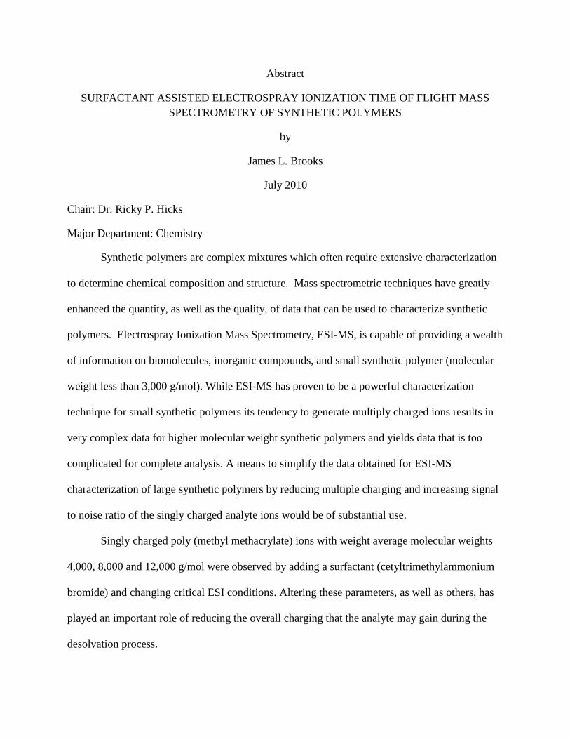
Abstract SURFACTANT ASSISTED ELECTROSPRAY IONIZATION TIME OF FLIGHT MASS SPECTROMETRY OF SYNTHETIC POLYMERS by James L. Brooks July 2010 Chair: Dr. Ricky P. Hicks Major Department: Chemistry Synthetic polymers are complex mixtures which often require extensive characterization to determine chemical composition and structure. Mass spectrometric techniques have greatly enhanced the quantity, as well as the quality, of data that can be used to characterize synthetic polymers. Electrospray Ionization Mass Spectrometry, ESI-MS, is capable of providing a wealth of information on biomolecules, inorganic compounds, and small synthetic polymer (molecular weight less than 3,000 g/mol). While ESI-MS has proven to be a powerful characterization technique for small synthetic polymers its tendency to generate multiply charged ions results in very complex data for higher molecular weight synthetic polymers and yields data that is too complicated for complete analysis. A means to simplify the data obtained for ESI-MS characterization of large synthetic polymers by reducing multiple charging and increasing signal to noise ratio of the singly charged analyte ions would be of substantial use. Singly charged poly (methyl methacrylate) ions with weight average molecular weights 4,000, 8,000 and 12,000 g/mol were observed by adding a surfactant (cetyltrimethylammonium bromide) and changing critical ESI conditions. Altering these parameters, as well as others, has played an important role of reducing the overall charging that the analyte may gain during the desolvation process.
Transcript of Abstract SPECTROMETRY OF SYNTHETIC...
Abstract
SURFACTANT ASSISTED ELECTROSPRAY IONIZATION TIME OF FLIGHT MASS
SPECTROMETRY OF SYNTHETIC POLYMERS
by
James L. Brooks
July 2010
Chair: Dr. Ricky P. Hicks
Major Department: Chemistry
Synthetic polymers are complex mixtures which often require extensive characterization
to determine chemical composition and structure. Mass spectrometric techniques have greatly
enhanced the quantity, as well as the quality, of data that can be used to characterize synthetic
polymers. Electrospray Ionization Mass Spectrometry, ESI-MS, is capable of providing a wealth
of information on biomolecules, inorganic compounds, and small synthetic polymer (molecular
weight less than 3,000 g/mol). While ESI-MS has proven to be a powerful characterization
technique for small synthetic polymers its tendency to generate multiply charged ions results in
very complex data for higher molecular weight synthetic polymers and yields data that is too
complicated for complete analysis. A means to simplify the data obtained for ESI-MS
characterization of large synthetic polymers by reducing multiple charging and increasing signal
to noise ratio of the singly charged analyte ions would be of substantial use.
Singly charged poly (methyl methacrylate) ions with weight average molecular weights
4,000, 8,000 and 12,000 g/mol were observed by adding a surfactant (cetyltrimethylammonium
bromide) and changing critical ESI conditions. Altering these parameters, as well as others, has
played an important role of reducing the overall charging that the analyte may gain during the
desolvation process.

© Copyright 2010
James Lee Brooks

SURFACTANT ASSISTED ELECTROSPRAY IONIZATION TIME OF FLIGHT MASS
SPECTROMETRY OF SYNTHETIC POLYMERS
A Thesis
Presented To
the Faculty of the Department of Chemistry
East Carolina University
In Partial Fulfillment
of the Requirements for the Degree
Master of Science in Chemistry
by
James L. Brooks
July, 2010

SURFACTANT ASSISTED ELECTROSPRAY IONIZATION TIME OF FLIGHT MASS
SPECTROMETRY OF SYNTHETIC POLYMERS
by
James L. Brooks
APPROVED BY:
DIRECTOR OF THESIS: ________________________________________________________
Timothy J. Romack, PhD
COMMITTEE MEMBER: _______________________________________________________
Colin S. Burns, PhD
COMMITTEE MEMBER: _______________________________________________________
Paul W. Hager, PhD
COMMITTEE MEMBER: _______________________________________________________
Yumin Li, PhD
CHAIR OF THE DEPARTMENT OF CHEMISTRY:
________________________________________________________
Ricky P. Hicks, PhD
DEAN OF THE GRADUATE SCHOOL:
________________________________________________________
Paul J. Gemperline, PhD

ACKNOWLEDGEMENTS
I would like to thank my research advisor for helping me get through those tough
semesters and guiding me from the beginning to the end of my research. Also, I would like to
thank my committee members for being supportive throughout my project.
I would like to thank the Department of Chemistry for accepting me into their graduate
program, providing me with the necessary tools to carry out my research, and financially
supporting me.
Finally, to my family, thank you for teaching me that with hard work and determination I
could get through anything.

TABLE OF CONTENTS
LIST OF TABLES ........................................................................................................................ vii
LIST OF FIGURES ..................................................................................................................... viii
LIST OF SCHEMES....................................................................................................................... x
LIST OF EQUATIONS ................................................................................................................. xi
LIST OF ABBREVIATIONS ....................................................................................................... xii
CHAPTER 1: BACKGROUND ..................................................................................................... 1
1.1 Brief History of Synthetic Polymers ..................................................................................... 1
1.2 Introduction to Synthetic Polymers ....................................................................................... 2
1.3 Typical Techniques of Analysis ............................................................................................ 4
1.4 Overview of Mass Spectrometry ........................................................................................... 7
1.4.1 Ionization Source ............................................................................................................ 7
1.4.2 Mass Analyzer ................................................................................................................ 8
1.5 Overview of ESI-MS ............................................................................................................. 9
1.5.1 Production of Gas Phase Ions from Charged Droplets ................................................. 10
1.6 What We Know About ESI-MS .......................................................................................... 11
1.7 Surfactants ........................................................................................................................... 13
1.8 ESI-MS of Synthetic Polymers ........................................................................................... 14
CHAPTER 2: ELECTROSPRAY IONIZATION OF POLY (METHYL METHACRYLATE) 16
2.1 Results and Discussion ........................................................................................................ 16

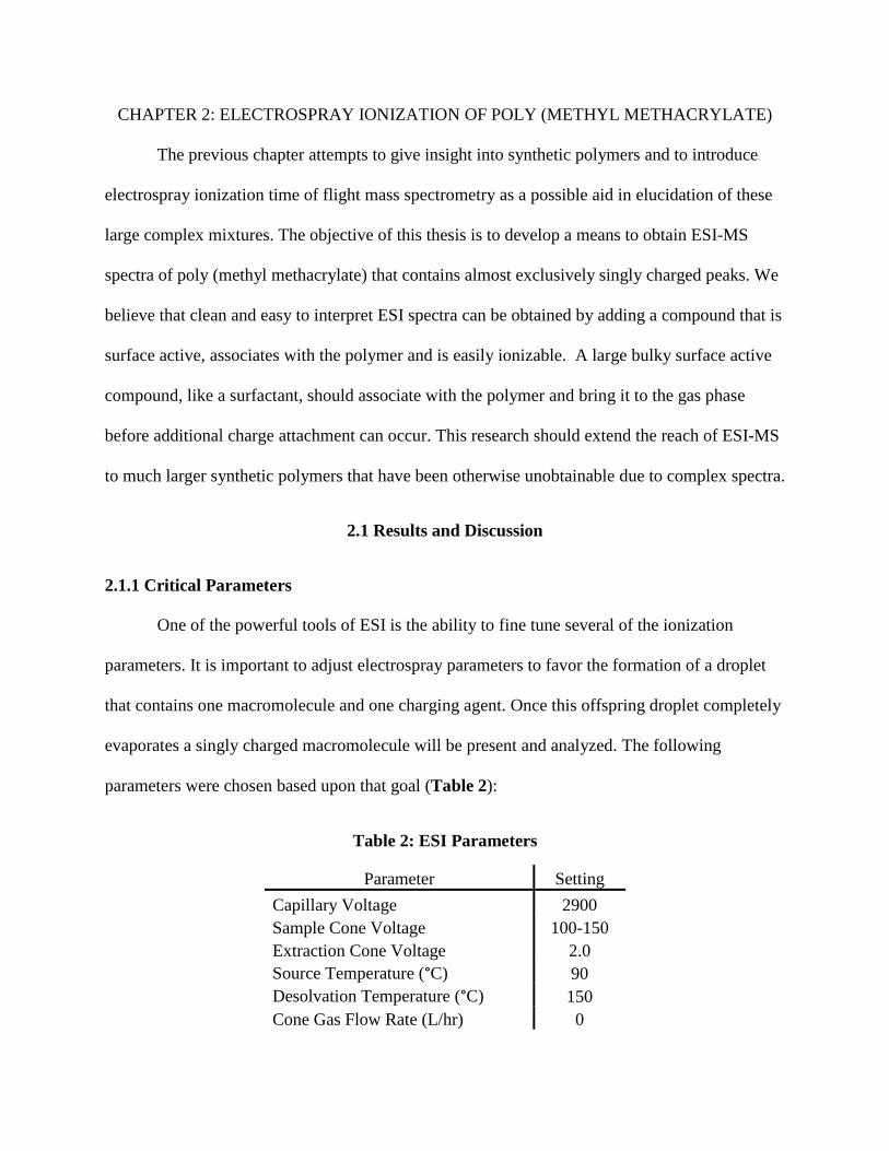
2.1.1 Critical Parameters ....................................................................................................... 16
2.1.2 Solvent Selection .......................................................................................................... 20
2.2 ESI-MS of Poly (Methyl Methacrylate) .............................................................................. 20
2.2.1 Analysis of PMMA 4000 .............................................................................................. 21
2.2.2 Analysis of PMMA 8000 .............................................................................................. 30
2.2.3 Analysis of PMMA 12000 ............................................................................................ 36
2.3 Surfactant Consideration ..................................................................................................... 43
2.4 Conclusion and Suggestions for Future Work .................................................................... 45
CHAPTER 3: EXPERIMENTAL................................................................................................. 47
3.1 Materials .............................................................................................................................. 47
3.2 GPC Polystyrene Sample Preparation and Calibration ....................................................... 47
3.2.1 PMMA Standard Sample Preparation and Analysis for GPC ...................................... 48
3.3 ESI-ToF Sample Preparation .............................................................................................. 48
3.3.2 ESI Parameters for Each Sample .................................................................................. 50
3.4 NMR Sample Preparation ................................................................................................... 52
APPENDIX A. Calibration of PMMA 4000. ............................................................................... 56
APPENDIX B. Calibration of PMMA 8000................................................................................. 59
APPENDIX C. Calibration of PMMA 12000............................................................................... 62
APPENDIX D. Spectrum and Parameters of PMMA 4000 with Cetyltrimethylammonium
Bromide......................................................................................................................................... 65

APPENDIX E. Spectrum and Parameters of PMMA 4000 with Dihexadecyldimethylammonium
Bromide......................................................................................................................................... 66
Appendix F. Spectrum and Parameters of PMMA 4000 with Tetrahexadecylammonium
Bromide......................................................................................................................................... 67

LIST OF TABLES
Table 1: Synthetic Polymer Applications ....................................................................................... 4
Table 2: ESI Parameters................................................................................................................ 16
Table 3: The actual m/z, intensity, and corrected m/z of PMMA 4000........................................ 24
Table 4: Molecular weight distribution data from ESI-ToF calculations, In-Lab GPC, and
Manufacturer GPC of PMMA 4000 ............................................................................................. 25
Table 5: Assigned Possible Structures to Peaks of PMMA 4000 ................................................. 27
Table 6: The actual m/z, intensity, and corrected m/z of PMMA 8000........................................ 32
Table 7: Molecular weight distribution data from ESI-ToF calculations, In-Lab GPC, and
Manufacturer GPC of PMMA 8000 ............................................................................................. 34
Table 8: PMMA 8000 Assigned Structures of Major Species ...................................................... 34
Table 9: The actual m/z, intensity, and corrected m/z of PMMA 12000...................................... 40
Table 10: Molecular weight distribution data from ESI-ToF calculations, In-Lab GPC, and
Manufacturer GPC of PMMA 12000 ........................................................................................... 41
Table 11: PMMA 12000 Assigned Structures of Major Species .................................................. 42

LIST OF FIGURES
Figure 1: Possible Distribution of Molecular Sizes of a Polymer Sample ..................................... 2
Figure 2: Poly (methyl methacrylate) ............................................................................................. 2
Figure 3: Example of ESI MS Multiple Charging of a Synthetic Polymer Sample ....................... 6
Figure 4: Components of a Typical Mass Spectrometer ................................................................. 7
Figure 5: ESI Process .................................................................................................................... 10
Figure 6: Charge Residue Mechanism .......................................................................................... 10
Figure 7: Ion Evaporation Mechanism ......................................................................................... 11
Figure 8: Surface Active Analytes have a Higher ESI Response ................................................. 13
Figure 9: Cetyltrimethylammonium Bromide .............................................................................. 13
Figure 10: Internal Scheme of Electrospray ................................................................................. 17
Figure 11: ESI-ToF of PMMA 4000 without a cationizing agent at optimized parameters......... 21
Figure 12: ESI-ToF of PMMA 4000 with the addition of cetyltrimethylammonium bromide
under optimized conditions ........................................................................................................... 23
Figure 13: Calibration lines generated from corrected and actual ESI data points ...................... 24
Figure 14: NMR of PMMA 4000 ................................................................................................. 30
Figure 15: ESI-ToF of PMMA 8000 without a cationizing agent at optimized parameters......... 31
Figure 16: ESI-ToF of PMMA 8000 with the addition of cetyltrimethylammonium bromide
under optimized conditions ........................................................................................................... 32
Figure 17: NMR of PMMA 8000 ................................................................................................. 36
Figure 18: ESI-ToF of PMMA 12000 without a cationizing agent at optimized parameters ....... 37
Figure 19: ESI-ToF of PMMA 12000 with the addition of cetyltrimethylammonium bromide
under optimized conditions ........................................................................................................... 38
Figure 20: Expansion of the singly charged region from the ESI-ToF of PMMA 12000 with the
addition of cetyltrimethylammonium bromide under optimized conditions ................................ 39
Figure 21: Cetyltrimethylammonium Bromide ............................................................................ 44
Figure 22: Dihexadecyldimethylammonium Bromide ................................................................. 44
Figure 23: Tetrahexadecylammonium Bromide ........................................................................... 44

LIST OF SCHEMES
Scheme 1: Group Transfer Polymerization Mechanism ............................................................... 29
LIST OF EQUATIONS
Equation 1: Weight Average Molecular Weight ............................................................................ 3
Equation 2: Number Average Molecular Weight ........................................................................... 3
Equation 3: Poly Dispersity ............................................................................................................ 3
Equation 4: Concentration of Excess Charge ............................................................................... 19
Equation 5: Percent Difference ..................................................................................................... 26

LIST OF ABBREVIATIONS
Mw Weight Average Molecular Weight
Mn Number Average Molecular Weight
PD Polydispersity
GPC Gel Permeation Chromatography
MALS Multi Angel Laser Light Scattering
NMR Nuclear Magnetic Resonance
MALDI Matrix-Assisted Laser Desorption / Ionization
ESI Electrospray Ionization
MS Mass Spectrometry
m/z Mass to Charge Ratio
DNA Deoxyribonucleic Acid
EI Electron Impact
CI Chemical Ionization
ToF Time of Flight
CRM Charge Residue Mechanism
IEM Ion Evaporation Mechanism
V Voltage
C Celsius
µL Microliter
Q Concentration of Excess Charge
i Circuit Current
F Faraday Constant

Γ Flow Rate
xc Calculated PMMA Peak Mass to Charge Ratio Values
xa Actual PMMA Peak Mass to Charge Values
CHAPTER 1: BACKGROUND
“Polymers are composed of covalent structures many times greater in extent
than those occurring in simple compounds and this feature alone accounts
for the characteristic properties that set them apart from other forms of
matter. Appropriate means need to be used to elucidate their macromolecular
structure and relationships established to express the dependence of physical
and chemical properties on the structures so evaluated.” – Paul Flory [1]
1.1 Brief History of Synthetic Polymers
Since the beginning of time polymers have existed as natural bio-molecules which are
essential to life. The manufacture of synthetic polymers has been applied to a wide range of
applications: cable insulation, car parts, packaging chips, kitchen appliances, paints, etc. The first
published examples of synthetic polymers were vulcanized rubber and Bakelite. In the early
1800’s natural rubber was an important commodity to the world but consequently it could only
be used in limited environments because the natural rubber would become brittle if it became too
cold or melt if it became too hot. In 1839 Charles Goodyear stumbled upon the synthesis of
rubber that made it weather proof and the synthesis was given the title vulcanization [2]. In 1907
Leo Baekeland synthesized Bakelite, also known as polyoxybenzylmethylenglycolanhydride,
which was important for its ability to act as an electrical insulator and its resistance to heat [3].
Up until the 1920’s little was known about these large interconnected compounds
(macromolecules) or if they were even interconnected, but Hermann Staudinger proved the
existence of macromolecules with x-ray studies [4]. Staudinger was awarded the Nobel Prize in
2
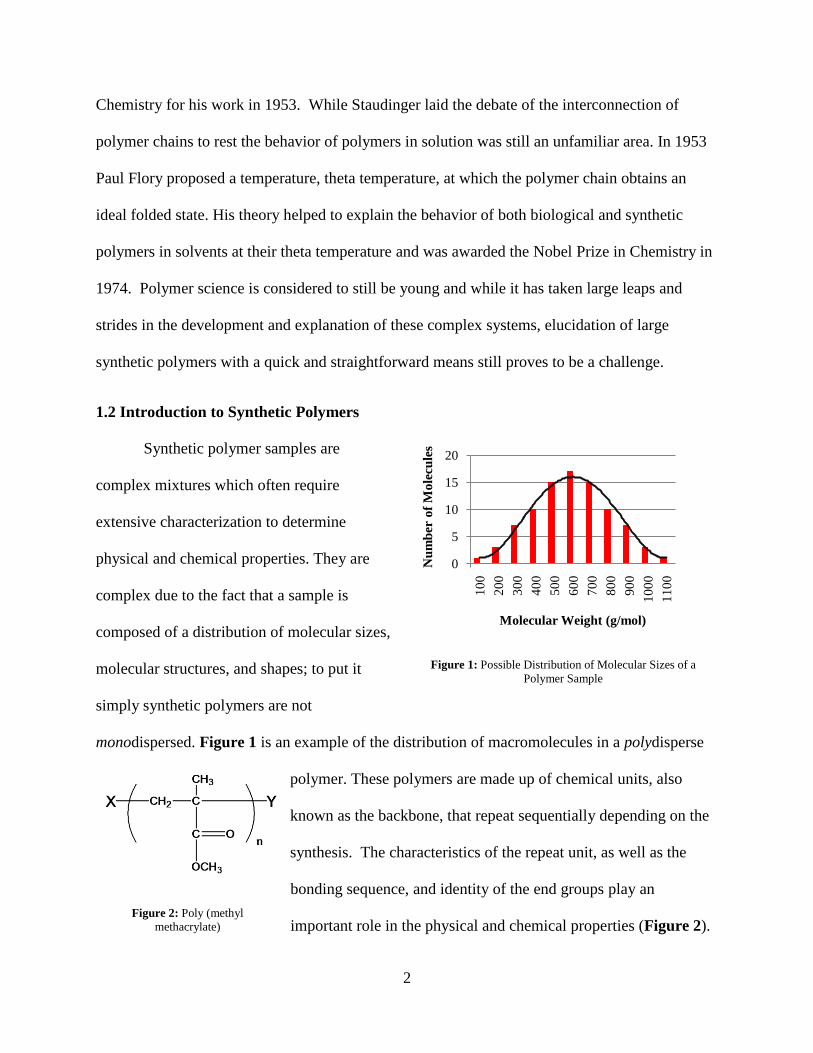
Chemistry for his work in 1953. While Staudinger laid the debate of the interconnection of
polymer chains to rest the behavior of polymers in solution was still an unfamiliar area. In 1953
Paul Flory proposed a temperature, theta temperature, at which the polymer chain obtains an
ideal folded state. His theory helped to explain the behavior of both biological and synthetic
polymers in solvents at their theta temperature and was awarded the Nobel Prize in Chemistry in
1974. Polymer science is considered to still be young and while it has taken large leaps and
strides in the development and explanation of these complex systems, elucidation of large
synthetic polymers with a quick and straightforward means still proves to be a challenge.
1.2 Introduction to Synthetic Polymers
Synthetic polymer samples are
complex mixtures which often require
extensive characterization to determine
physical and chemical properties. They are
complex due to the fact that a sample is
composed of a distribution of molecular sizes,
molecular structures, and shapes; to put it
simply synthetic polymers are not
monodispersed. Figure 1 is an example of the distribution of macromolecules in a polydisperse
polymer. These polymers are made up of chemical units, also
known as the backbone, that repeat sequentially depending on the
synthesis. The characteristics of the repeat unit, as well as the
bonding sequence, and identity of the end groups play an
important role in the physical and chemical properties (Figure 2).
0
5
10
15
20
10
0
20
0
30
0
40
0
50
0
60
0
70
0
80
0
90
0
10
00
11
00
Nu
mb
er o
f M
ole
cule
s
Molecular Weight (g/mol)
Figure 1: Possible Distribution of Molecular Sizes of a
Polymer Sample
Figure 2: Poly (methyl
methacrylate)

3
The n in Figure 2 represents the degree of polymerization, which corresponds to chain length of
the polymer. Chain length of a polymer is important for its interactions with itself and with other
compounds. In order to help describe these complex systems polymer chemist use weight
average molar mass (Mw) (Equation 1), number average molar mass (Mn) (Equation 2), and
polydispersity (PD) (Equation 3). The weight average molar mass takes into account the mass-
average probability per molecule that a given macromolecule is present in the sample. The
number average molar mass is the molecule number-average probability that a given
macromolecule mass is present in the sample. Polydispersity is an index which utilizes both the
weight average molar mass and number average molar mass help to describe how narrow or
broad the polymer molecular mass distribution is.
Equation 1: Weight Average Molecular Weight
Mw = ΣiNiMi2 / ΣiNiMi
Equation 2: Number Average Molecular Weight
Mn = ΣiNiMi / ΣiNi
Equation 3: Poly Dispersity
PD = Mw / Mn
Where N in equations 1 and 2 represents the number of molecules, M is the molar mass of
the ith
molecules, and i is the selected molecule.
Synthetic polymers can be tailored to exist as hydrophobic, hydrophilic, high or low
molecular weight, transparent, opaque, energy resilient, energy absorbing or any combination of
these properties. All of these characteristics can be controlled by manipulating the chemical and

4
physical properties which are greatly influenced by molecular weight, molecular weight
distribution, chemical composition, chemical composition distribution, topology and end groups.
Due to the wide range of properties that polymers can have they make up a broad range
of many day to day applications that extends
from household goods to industrial tools.
Some of the synthetic polymers that have
proven to be of relevant importance include
Kevlar (poly paraphenylene terephthalamide) which is used in body armor, polyvinyl chloride’s
which are commonly used for insulation and fluoropolymer’s in lubricants. For more examples
of relevant synthetic polymers see Table 1. These synthetic polymers, as well as many more,
have made life much safer and more efficient. Challenging polymer samples can require
extensive characterization utilizing various analytical techniques to determine the aspects which
account for their distinct properties.
1.3 Typical Techniques of Analysis
As discussed earlier the broad range of properties of synthetic polymers can require
comprehensive characterization in order to identify the important physical and chemical
characteristics, which make their applications unique. It is important to reveal these key factors
governing the physical and chemical characteristics in order to understand the synthetic
polymer’s functions. Insight into these characteristics can be explained by obtaining data on the
chemical composition, chemical composition distribution, molecular weight, molecular weight
distribution, topology, and end groups. Common techniques for the characterization of synthetic
polymers include gel permeation chromatography (GPC) / multi angle laser light scattering
Chemical Name Application
Poly (methyl methacrylate) Automotive Parts
Polytetrafluoroethylene Teflon
Polyethylene House Appliances
Polystyrene Packaging Chips
Table 1: Synthetic Polymer Applications

5
(MALS), nuclear magnetic resonance (NMR), matrix-assisted laser desorption/ionization mass
spectrometry (MALDI-MS), and electrospray ionization mass spectrometry (ESI-MS).
GPC separates polymer samples into several fractions which are then analyzed by one or
more detectors (i.e. refractive index, ultraviolet detector, MALS). While GPC has proven to be a
very important tool in yielding data on the weight average molecular weight, number average
molecular weight and polydispersity of polymers, end group determination is not yet possible.
End group determination of synthetic polymers is vital in that it contributes to the performance
properties as well as reactivity.
NMR is capable of measuring the molecular weight and determining end groups of
synthetic polymers, however determination of these two properties can only be elucidated under
certain circumstances. As the length of the backbone increases (we can relate the overall length
of the chain to the overall concentration of the sum of the backbone units) the concentration of
the end group’s decreases which directly affects the NMR signal strength.
MALDI-MS strength lies in its ability to singly charge large synthetic polymers creating
simple and easy to interpret spectra. However, while MALDI-MS is considered to be a soft
ionization technique it has been shown to fragment polymer end groups [5]. Soft ionization
refers to a mass spectrometers ability to induce little, if any, fragmentation and minor loss non-
covalent interaction. MALDI requires that the mixture of a matrix and analyte are soluble in a
solvent so they can co-crystallize, however this can prove to be difficult with the available
matrixes. Also, MALDI is not easily coupled to separation methods (i.e. high pressure liquid
chromatography, capillary electrophoresis, and GPC) due to it being a pulsed ionization
technique (produces packets of ions, not a continuous flow of ions).
6
ESI-MS has proven to be a very powerful technique in analyzing smaller synthetic
polymers (i.e. molecular weight < 3,000 g/mol) yielding data on chemical composition,
molecular weight, molecular weight distribution, and end groups [6, 7]. Multiple charging of
analytes is considered to be a powerful feature for analyzing biomolecules, such as proteins and
deoxyribonucleic acid (DNA), but this feature greatly limits the ability of ESI to characterize
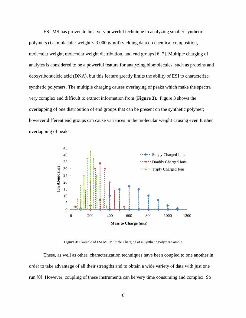
synthetic polymers. The multiple charging causes overlaying of peaks which make the spectra
very complex and difficult to extract information from (Figure 3). Figure 3 shows the
overlapping of one distribution of end groups that can be present on the synthetic polymer;
however different end groups can cause variances in the molecular weight causing even further
overlapping of peaks.
Figure 3: Example of ESI MS Multiple Charging of a Synthetic Polymer Sample
These, as well as other, characterization techniques have been coupled to one another in
order to take advantage of all their strengths and to obtain a wide variety of data with just one
run [8]. However, coupling of these instruments can be very time consuming and complex. So
0
5
10
15
20
25
30
35
40
45
0 200 400 600 800 1000 1200
Ion
Ab
un
da
nce
Mass to Charge (m/z)
Singly Charged Ions
Doubly Charged Ions
Triply Charged Ions
7
while all of these characterization techniques have their strengths they have a core weakness that
limits the amount of information which can be gathered from synthetic polymers. ESI-MS
seems to be an appealing candidate for the analysis of larger molecular weight synthetic
polymers if the charge state distribution could be controlled.
1.4 Overview of Mass Spectrometry
It is a common misconception that mass spectrometers measure the actual molecular
weight of a compound, they actually measure the mass to charge ratio (m/z) versus the ion
abundance. As a result of individual ions being measured the isotope effect must be accounted
for and not an averaged mass. For example bromine has two naturally occurring isotopes 79
Br
(natural abundance 50.7% and 78.92 g/mol) and 81
Br (natural abundance 49.3% and 80.92
g/mol) so two separate peaks will be detected at 78.92 and 80.92 m/z with the former peak
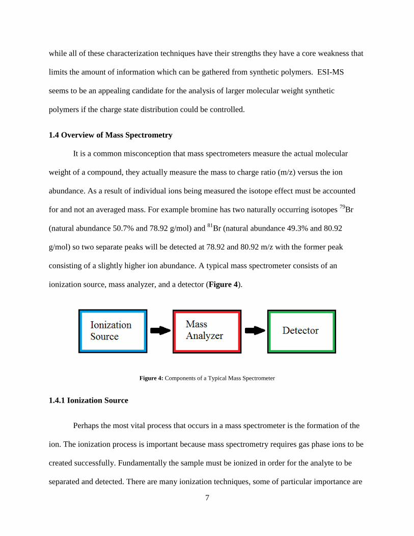
consisting of a slightly higher ion abundance. A typical mass spectrometer consists of an
ionization source, mass analyzer, and a detector (Figure 4).
Figure 4: Components of a Typical Mass Spectrometer
1.4.1 Ionization Source
Perhaps the most vital process that occurs in a mass spectrometer is the formation of the
ion. The ionization process is important because mass spectrometry requires gas phase ions to be
created successfully. Fundamentally the sample must be ionized in order for the analyte to be
separated and detected. There are many ionization techniques, some of particular importance are
8
electron impact (EI), chemical ionization (CI), matrix-assisted laser desorption/ionization
(MALDI), and electrospray ionization (ESI). The first technique, EI, is considered to be a hard
ionization technique (causes loss of covalent and non-covalent interaction) which is not optimal
for acquiring reliable data on end groups and molecular weight distribution information. Also
when using EI or CI the analyte must be volatile, thermally stable, and have a molecular weight
less than 1,000 g/mol. MALDI and ESI are soft ionization techniques that permit the ionization
of large nonvolatile compounds, like synthetic polymers.
1.4.2 Mass Analyzer
It is advantageous to be familiar with the molecular mass range of your analyte when
selecting a mass analyzer because many mass analyzers have a set mass to charge range. Linear
quadrupole and quadrupole ion traps mass to charge ranges do not exceed 6,000 m/z. This is not
a crucial factor when working with low molecular weight compounds or when multiple charging
higher molecular weight compounds that are monodisperse, but synthetic polymers can be very
large well exceeding the mass of 6,000 g/mol. It is also important to note once again that
synthetic polymers have a distribution of sizes and molecular weights associated with the
sample, so the mass spectra will not have just one peak, it will have a distribution of peaks that
vary over a large mass to charge range. The Time-of-Flight (ToF) mass analyzer has proven to
be a very powerful ally when analyzing larger molecular weight compounds due the fact that the
mass to charge range is theoretically unlimited.
Mass spectrometric techniques have significantly enhanced the quantity, as well as the
quality, of data that can be obtained from many classes of compounds (i.e. catalyst, proteins,
carbohydrates, etc.). Sensitivity, reproducibility, and automation have been established to be
some of the features that make mass spectrometry so powerful. Mass spectrometry encompasses

9
a broad range of applications in fields such as inorganic chemistry, physical chemistry,
biochemistry, medical chemistry, etc. However, the successful and complete elucidation of large
synthetic polymers still proves to be an issue that has yet to be resolved.
1.5 Overview of ESI-MS
Electrospray was first investigated by Malcolm Dole over four decades ago [9], but was
not brought to the analytical realm until 1984 by John Fenn [10]. Fenn was able to analyze low
molecular weight analytes on an electrospray ionization quadrupole mass analyzer. In 2002 the
Noble Prize in Chemistry was awarded to John Fenn and Koichi Tanaka for their work in the soft
ionization techniques ESI and MALDI [11]. Their developments led to the analysis of higher
molecular weight compounds that were both non-volatile and thermally labile.
While the process of ESI is straightforward it is important to understand how charge
droplets are formed. A dilute sample (1-5 µM) is pushed through a capillary which has a high
voltage (2 – 5 kV) applied to it. The high voltage causes a separation of positive and negative
charges in solution. As the sample exits the capillary a Taylor cone is formed. Ions in solution
eventually experience enough repulsive force to overcome the surface tension of the solvent and
leave tip of the Taylor cone as a droplet. The droplets receive a push / pull to the mass analyzer
from the applied electric field depending on the voltage implemented (Figure 5). Positive
voltage at the capillary is typically applied for analyzing analytes that form positive ions, where
as negative voltage at the capillary is typically applied for analyzing analytes that form negative
ions [12].

10
Figure 5: ESI Process
1.5.1 Production of Gas Phase Ions from Charged Droplets
There are two processes that have been proposed which explain how gas phase analyte
ions form from charged droplets. After the droplet has ejected from the capillary it begins to
travel towards the mass analyzer and the solvent starts to evaporate during which the charged
residue mechanism (CRM) [9] or the ion evaporation model (IEM) [13] will be responsible for
the production of gas phase ions. The mechanism by which the analyte is ejected into the gas
phase is believed to be largely related to the analytes molecular size [14].
The charge residue mechanism
is believed to be the mechanism of gas
phase ion formation of larger
compounds. As the droplet evaporates
it eventually reaches a point where the
surface charge density is great enough for the droplet to undergo fission, this point is referred to
as the Rayleigh limit [15]. The fission that takes place produces several offspring droplets from
Figure 6: Charge Residue Mechanism

11
the parent droplet, this process is repeated until one analyte molecule is present in one droplet, at
this point the solvent evaporates and the analyte is released into the gas phase (Figure 6).
The ion evaporation model is
believed to govern the gas phase ion
formation for smaller compounds. During
the IEM the droplet undergoes similar
evaporation and fission events to that of
CRM; however at a critical diameter in the evaporation process coulombic repulsion forces the
analyte to eject from the droplet surface to the gas phase in its ion form (Figure 7).
The CRM and IEM are different in the way by which the analyte in the droplet is released
to the gas phase as ions. We are more interested in the charge residue mechanism (CRM)
because the synthetic polymers that we wish to analyze are considered to be large compounds.
1.6 What We Know About ESI-MS
Solvent selection plays an important role in the observed analyte charge state. Multiple
charging of the analyte in the positive ion mode results from the attachment of several protons or
several cations. Use of higher polarity solvents has been shown to favor the formation of higher
charge states because it improves stability of charge separation in solution [16]. Improved
stability of charge separation in solution can hinder the ability of the counterion to move to the
parent and offspring droplets during the droplet fission process. This decreases the overall ion
pairing during the solvent evaporation and droplet fission process.
The range of solvents in ESI is limited to those with higher dielectric constants (20 - 80).
This is due to the fact that ESI solvents must be capable of conducting charge. Typically with an
Figure 7: Ion Evaporation Mechanism
12
increase in the dielectric constant of the solvent the surface tension also increases. It has been
seen that if the surface tension of the solvent is increased the charge state of the analyte will also
be increased [17]. The surface tension increases the time it takes the droplet to reach the
Rayleigh limit which effectively enhances the amount of charges that can exist on the surface of
the droplet before fission occurs. This will result in higher concentration of charges in the
offspring droplet. The rise in the number of charges that will exist in the droplet surface
increases the likely hood for the analyte to obtain more than one charge as it enters the gas phase.
It is also important to note the solubility of analytes in the solvent, i.e. better solvated ions have
lower partitioning constants and hence will have a lower ESI response [18].
Analytes with the highest response have been shown to have both a polar and a nonpolar
character. The polar portion can help to facilitate charging while the nonpolar character of an
analyte causes it to exist on the surface of the droplet. This is because the solvents typically
employed are polar so the partitioning constant of the nonpolar character will be higher than that
of a analyte with a large polar character [19]. Also the atmospheric environment of the droplet is
considered to be nonpolar, so the analyte will partition to the nonpolar phase. Analytes that
exhibit a higher degree of surface activity will have higher intensity signals because these surface
active analytes exhibit greater desorption characteristics [20] (Figure 8). Figure 8 shows how a
surface active compound (A) has a much greater probability of being in the offspring droplet
during the fission process then a compound that exists in the core of the droplet (B).

13
Figure 8: Surface Active Analytes have a Higher ESI Response
1.7 Surfactants
Surfactants are surface active compounds that contain a polar (hydrophilic) head and a
nonpolar (hydrophobic) tail, this property of a compound is also typically identified as being
amphiphlic (Figure 9). Surfactants have a broad range of usages and can be found in various
products such as detergents, shampoos, paints, and dental floss. They are soluble in nonpolar and
polar environments, which allow it to act as a phase interface transferring agent. However to our
knowledge the unique and diverse range of properties that are derived from there amphiphlic
character has not been applied to ESI-MS of synthetic polymers. Based on the literature it is
believed that certain surfactants will have a very high ESI response even at a low concentration
due to the nonpolar character and its ability to have a stable charge. If a surfactant is able to
associate with an analyte acting as the charging agent then it may be brought to the surface of the
droplet.
Figure 9: Cetyltrimethylammonium Bromide
14
1.8 ESI-MS of Synthetic Polymers
ESI-MS is considered to be a very soft ionization technique that limits the amount of
fragmentation and decomposition of synthetic polymers. The limited amount of decomposition
and fragmentation that takes place allows for the reliable determination of end groups and
molecular weight distribution data. While this feature of ESI is advantageous for lower
molecular weight polymers, larger molecular weight polymers are still plagued by the multiple
charging that occurs which creates spectral congestion due to peak overlap.
As stated earlier ESI has a limited solvent selection, depending on the analyte being
analyzed, due to conductivity requirements. Typical ESI solvents include, but are not limited to,
methanol, acetonitrile, and water. Various solvents can be mixed and matched to meet suitable
conductivity requirements, but solubility of the analyte can still be an obstacle here. Most
industrial and household synthetic polymers are nonpolar and require such solvents to be
dissolved in. Researchers have utilized additives that act as conductivity enhancers to attempt to
deal with this polymer solubility and solvent conductivity issue [21]. However, the lower m/z
region is congested by the conductivity enhancer and this does not deal with the issue of complex
spectra that are created by multiple charging.
A powerful feature of ESI is the ability to carefully modify the amount of energy that can
be imparted to the analyte. The potential that is applied to the capillary is one of the essential
parameters to obtaining a sustainable Taylor cone. It was seen that high cone voltage produced
higher intensity spectra of the lower molecular weight singly charged synthetic polymer ions
[22]. Larger gas phase ions of lower charge states do not experience the same amount of
focusing towards the skimmer. The increased energy imparted to the analyte also promotes
15
charge shedding. Charge shedding is the transfer of charge from the analyte to neutral gas
molecules or species that were present in the sample and solvent.
To our knowledge ESI-ToF-MS has not been utilized to successfully analyze poly(methyl
methacrylate) samples above the mass range of 4,000 g/mol without an offline/online separation
technique or data processing assistance [23].
CHAPTER 2: ELECTROSPRAY IONIZATION OF POLY (METHYL METHACRYLATE)
The previous chapter attempts to give insight into synthetic polymers and to introduce
electrospray ionization time of flight mass spectrometry as a possible aid in elucidation of these
large complex mixtures. The objective of this thesis is to develop a means to obtain ESI-MS
spectra of poly (methyl methacrylate) that contains almost exclusively singly charged peaks. We
believe that clean and easy to interpret ESI spectra can be obtained by adding a compound that is
surface active, associates with the polymer and is easily ionizable. A large bulky surface active
compound, like a surfactant, should associate with the polymer and bring it to the gas phase
before additional charge attachment can occur. This research should extend the reach of ESI-MS
to much larger synthetic polymers that have been otherwise unobtainable due to complex spectra.
2.1 Results and Discussion
2.1.1 Critical Parameters
One of the powerful tools of ESI is the ability to fine tune several of the ionization
parameters. It is important to adjust electrospray parameters to favor the formation of a droplet
that contains one macromolecule and one charging agent. Once this offspring droplet completely
evaporates a singly charged macromolecule will be present and analyzed. The following
parameters were chosen based upon that goal (Table 2):
Table 2: ESI Parameters
Parameter Setting
Capillary Voltage 2900
Sample Cone Voltage 100-150
Extraction Cone Voltage 2.0
Source Temperature (°C) 90
Desolvation Temperature (°C) 150
Cone Gas Flow Rate (L/hr) 0
17
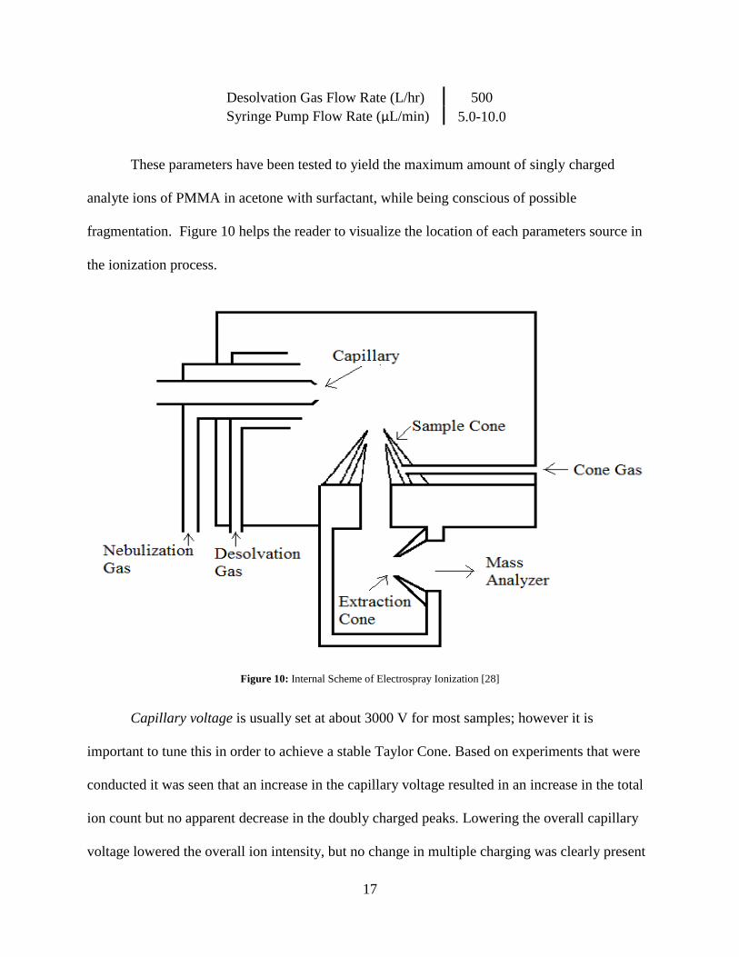
Desolvation Gas Flow Rate (L/hr) 500
Syringe Pump Flow Rate (µL/min) 5.0-10.0
These parameters have been tested to yield the maximum amount of singly charged
analyte ions of PMMA in acetone with surfactant, while being conscious of possible
fragmentation. Figure 10 helps the reader to visualize the location of each parameters source in
the ionization process.
Figure 10: Internal Scheme of Electrospray Ionization [28]
Capillary voltage is usually set at about 3000 V for most samples; however it is
important to tune this in order to achieve a stable Taylor Cone. Based on experiments that were
conducted it was seen that an increase in the capillary voltage resulted in an increase in the total
ion count but no apparent decrease in the doubly charged peaks. Lowering the overall capillary
voltage lowered the overall ion intensity, but no change in multiple charging was clearly present
18
as its ion intensity decreased along with the singly charged ion intensity. Increasing the capillary
voltage to a high setting can possibly cause fragmentation of the macromolecule so a capillary
voltage of 2900 was chosen.
The sample cone voltage is typically adjusted for the type of analyte being analyzed, i.e.
solvent, carbohydrates, protein ions, etc. Higher molecular weight analytes can require higher
sample cone voltage to observe appropriate distributions. Based on the ESI q-ToF manual the
sample cone voltage should be adjusted for maximum sensitivity, within the range 15V to 150V.
When increasing the sample cone voltage it is important be aware of possible analyte
fragmentation. Increasing the voltage leads to higher analyte kinetic energy which results in a
higher probability of collisions [24]. The sample cone voltage was adjusted for each sample to
achieve the maximum amount of singly charged ions.
Extractor cone voltage is typically optimizes within the range of 0 - 5V. Adjusting the
voltage to higher values may cause fragmentation of analyte ions. An extractor cone voltage of
2.0 appears to be appropriate for the poly (methyl methacrylate) standards.
Cone gas flow rate is typically altered to reduce the possible adduct ions or solvent
clustering ions. If the cone gas flow rate is set to 0 then it is possible to increase the length of
time that a low surface-charge density is present before droplet fission occurs, hence leading to
offspring droplets with less overall charge.
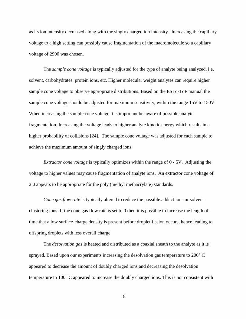
The desolvation gas is heated and distributed as a coaxial sheath to the analyte as it is
sprayed. Based upon our experiments increasing the desolvation gas temperature to 200° C
appeared to decrease the amount of doubly charged ions and decreasing the desolvation
temperature to 100° C appeared to increase the doubly charged ions. This is not consistent with

19
research that states that rapid evaporation of charged droplet should lead to higher charged states
[25]. However it is possible that the temperature is affecting the overall solubility of the polymer,
causing it to develop a closed or compact form. Also the increase of the viscosity of the droplet
would hinder the ability of the analyte to move to the surface and gain charge [26]. The
desolvation gas temperature was set to 150° C in order to diminish the amount of multiple
charging while keeping the amount of energy introduced to the system low enough to prevent
possible fragmentation.
In our studies of varying the gas desolvation flow rate it did not appear to alter the doubly
charged region or the ion intensity in any great effect. However, increasing the gas flow rate to
values higher than the amount quoted in the q-ToF manual leads to high nitrogen levels. High
levels of nitrogen could possibly cause an enhanced amount of collisions between the gas
molecules and analyte ions, but this is not likely. However, possible amplified amount of
collisions could cause charge shedding but could also induce fragmentation of labile groups.
The syringe pump flow rate is directly related to the amount sample consumed however
does not alter the amount of energy in the system. Increasing the syringe pump flow rate from
5.0 uL/min to 15.0 uL/min reduced the multiply charged region, as well as increased the overall
ion intensity. Based upon the literature using higher flow rates will create droplets with a lower
density of charge per unit volume [27].This can be explained by the excess charge equation listed
below:
Equation 4: Concentration of Excess Charge
[Q] = i / FΓ
20
Where [Q] represents the concentration of excess charge, i is the circuit current (amperes), F is
Faraday’s constant (96,485 coulomb/mol), and Γ is the flow rate (L/sec). Offspring droplets that
separate from the parent droplets when the surface charge density is low will contain fewer
charges [16]. The sample flow rate was adjusted for each sample as to optimize the amount of
sample consumed, the time it takes for successful analysis, and to reduce the amount of multiple
charging. For sample consumption purposes the syringe pump flow rate above 10.0 uL/min will
not be used as it produced a respectable ion intensity value as well as decreases the multiple
charging.
2.1.2 Solvent Selection
Selecting a solvent plays a considerable role in the conformation which a polymer
assumes in solution. We want a solvated polymer so isolated chains in solution form and the
polymer does not attach to one another forming large coalesced balls. A solvent that is not highly
polar and our analyte is soluble in would be suitable for ESI analysis. Acetone seems like an
appropriate candidate for our study with a low dielectric constant, compared to typical ESI
solvents (acetone at 21, methanol at 33, acetonitrile at 36, and water at 80), as well as a low
surface tension.
2.2 ESI-MS of Poly (Methyl Methacrylate)
Based upon the literature high molecular weight poly (methyl methacrylate) standards
have not yielded ESI-MS spectra dominated by singly charged ions. Poly (methyl methacrylate),
PMMA, has an extensive array of properties that can depend on its molecular weight, molecular
weight distribution, and end groups. PMMA can have good resistance to effects of weathering
while being a transparent tough material. This synthetic polymer has found applications in
lenses, skylight domes, protective coatings, and riot shields [29].
21
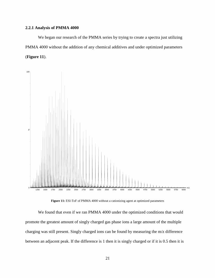
2.2.1 Analysis of PMMA 4000
We began our research of the PMMA series by trying to create a spectra just utilizing
PMMA 4000 without the addition of any chemical additives and under optimized parameters
(Figure 11).
Figure 11: ESI-ToF of PMMA 4000 without a cationizing agent at optimized parameters
We found that even if we ran PMMA 4000 under the optimized conditions that would
promote the greatest amount of singly charged gas phase ions a large amount of the multiple
charging was still present. Singly charged ions can be found by measuring the m/z difference
between an adjacent peak. If the difference is 1 then it is singly charged or if it is 0.5 then it is
m/z1250 1500 1750 2000 2250 2500 2750 3000 3250 3500 3750 4000 4250 4500 4750 5000 5250 5500 5750 6000
%
0
100
22
doubly charged. The large amount of multiple charging that takes place contributes to the overall
ion intensity of the singly charged peaks, [M + Cation]+, due to peak m/z overlapping.
Calculating the number average molecular weight, weight average molecular weight and
polydispersity will be perturbed by the overlapping ion intensity contribution. Also the
congestion in the lower ion intensity region requires additional deconvoluting to draw
information from. The lower intensity regions of these spectra can give insight into different end
groups of the polymer, possible contaminates present in the sample and/or other charging agents
present.
By adding our surfactant, cetyltrimethylammonium bromide, to the sample prior to
injection into the ESI-ToF, along with the optimized settings, we are able to create a spectrum
that is dominated by singly charged peaks, [M + CTA]+ that dwarfs the now lower ion intensity
doubly charged region (Figure 12).
23
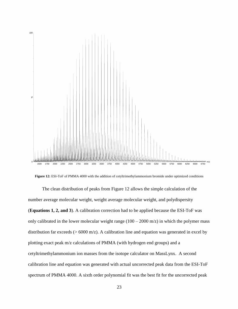
Figure 12: ESI-ToF of PMMA 4000 with the addition of cetyltrimethylammonium bromide under optimized conditions
The clean distribution of peaks from Figure 12 allows the simple calculation of the
number average molecular weight, weight average molecular weight, and polydispersity
(Equations 1, 2, and 3). A calibration correction had to be applied because the ESI-ToF was
only calibrated in the lower molecular weight range (100 – 2000 m/z) in which the polymer mass
distribution far exceeds (> 6000 m/z). A calibration line and equation was generated in excel by
plotting exact peak m/z calculations of PMMA (with hydrogen end groups) and a
cetyltrimethylammonium ion masses from the isotope calculator on MassLynx. A second
calibration line and equation was generated with actual uncorrected peak data from the ESI-ToF
spectrum of PMMA 4000. A sixth order polynomial fit was the best fit for the uncorrected peak
m/z1500 1750 2000 2250 2500 2750 3000 3250 3500 3750 4000 4250 4500 4750 5000 5250 5500 5750 6000 6250 6500 6750
%
0
100
24
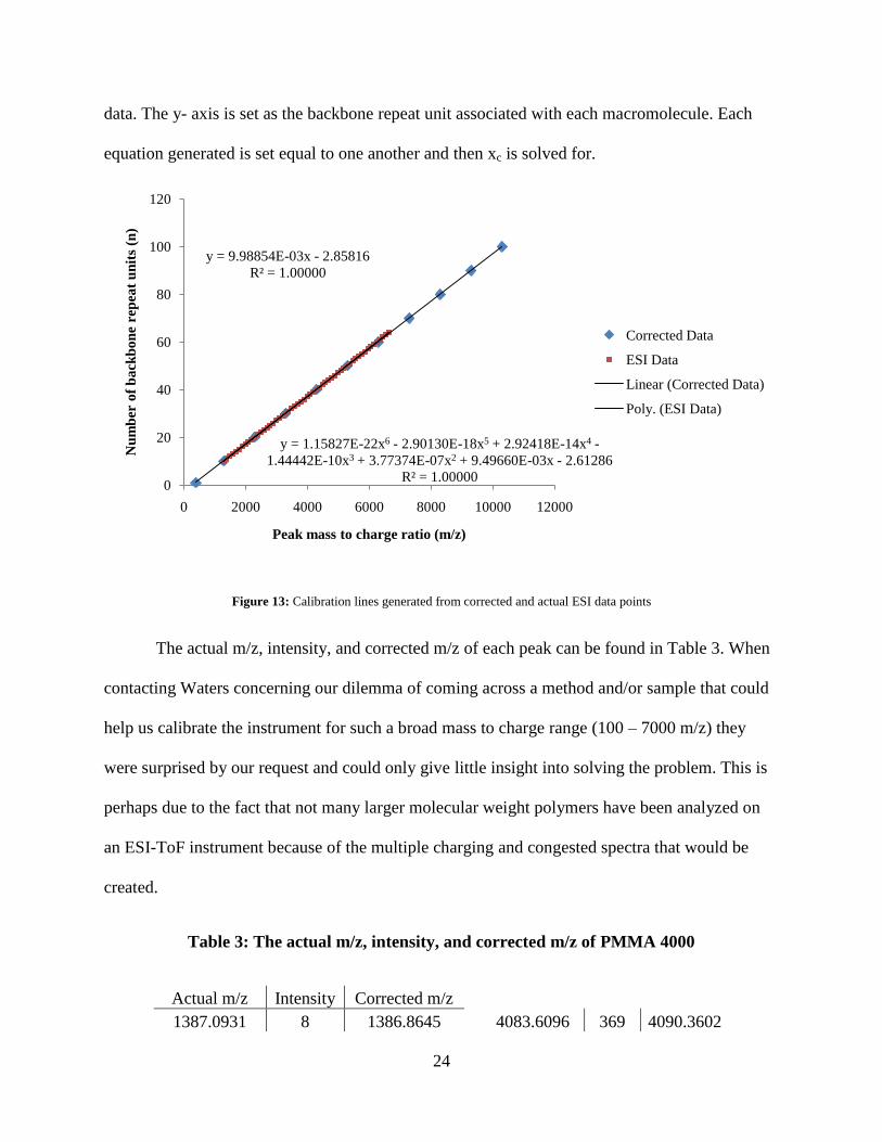
data. The y- axis is set as the backbone repeat unit associated with each macromolecule. Each
equation generated is set equal to one another and then xc is solved for.
Figure 13: Calibration lines generated from corrected and actual ESI data points
The actual m/z, intensity, and corrected m/z of each peak can be found in Table 3. When
contacting Waters concerning our dilemma of coming across a method and/or sample that could
help us calibrate the instrument for such a broad mass to charge range (100 – 7000 m/z) they
were surprised by our request and could only give little insight into solving the problem. This is
perhaps due to the fact that not many larger molecular weight polymers have been analyzed on
an ESI-ToF instrument because of the multiple charging and congested spectra that would be
created.
Table 3: The actual m/z, intensity, and corrected m/z of PMMA 4000
Actual m/z Intensity Corrected m/z 1387.0931 8 1386.8645
4083.6096 369 4090.3602
y = 9.98854E-03x - 2.85816
R² = 1.00000
y = 1.15827E-22x6 - 2.90130E-18x5 + 2.92418E-14x4 -
1.44442E-10x3 + 3.77374E-07x2 + 9.49660E-03x - 2.61286
R² = 1.000000
20
40
60
80
100
120
0 2000 4000 6000 8000 10000 12000
Nu
mb
er o
f b
ack
bo
ne
rep
eat
un
its
(n)
Peak mass to charge ratio (m/z)
Corrected Data
ESI Data
Linear (Corrected Data)
Poly. (ESI Data)

25
1487.1329 12 1486.7767
4182.7554 297 4190.3850
1588.1923 15 1587.7766
4281.8633 270 4290.4564
1688.2686 20 1687.8478
4380.8257 246 4390.4693
1788.3169 25 1787.9320
4479.7881 214 4490.5740
1888.3674 35 1888.0494
4579.5825 187 4591.6168
1988.3804 81 1988.1525
4678.3066 171 4691.6744
2088.4080 112 2088.2873
4775.9565 144 4790.7425
2188.4202 143 2188.4198
4875.5557 126 4891.8927
2288.4287 184 2288.5588
4974.0425 106 4992.0197
2388.3948 222 2388.6646
5072.1992 93 5091.9191
2488.3406 260 2488.7591
5169.6133 76 5191.1719
2588.2805 291 2588.8579
5268.5703 65 5292.1109
2688.1929 339 2688.9414
5366.6226 55 5392.2435
2788.0654 361 2789.0000
5464.6636 43 5492.4834
2887.8955 387 2889.0347
5561.9966 35 5592.1206
2987.4190 405 2988.7845
5659.5723 28 5692.1310
3087.5149 405 3089.1352
5756.2295 22 5791.3274
3187.2622 420 3189.1683
5854.2622 21 5892.0698
3286.9307 426 3289.1591
5952.5537 15 5993.2199
3387.6172 415 3390.2139
6049.7388 12 6093.3773
3487.1968 420 3490.2052
6145.5884 10 6192.3075
3586.7632 419 3590.2358
6243.1260 8 6293.1406
3686.2539 405 3690.2479
6339.5972 6 6393.0401
3785.6951 393 3790.2730
6437.2598 5 6494.3553
3885.0593 368 3890.2882
6532.5767 6 6593.4258
3984.3513 332 3990.3028
6628.0586 4 6692.8683
It is important to validate our molecular weight calculations from the ESI spectrum, so an In-lab
GPC on our PMMA 4000 standard was run and compared the values obtained (Table 4).
Table 4: Molecular weight distribution data from ESI-ToF calculations, In-Lab GPC, and
Manufacturer GPC of PMMA 4000
Technique Mw Mn PD
ESI - ToF 3480 3256 1.07
In-Lab GPC 3728 3497 1.07
Manufacturer GPC 4200 3900 1.06
26
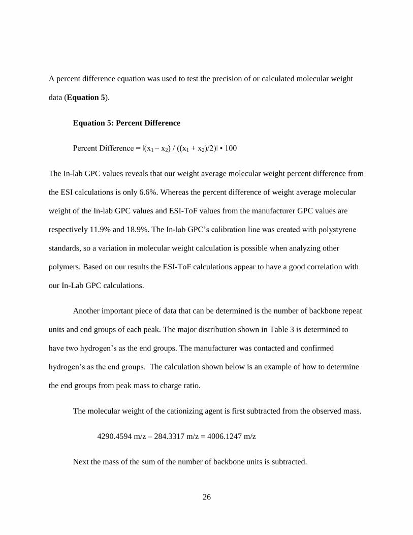
A percent difference equation was used to test the precision of or calculated molecular weight
data (Equation 5).
Equation 5: Percent Difference
Percent Difference = ǀ(x1 – x2) / ((x1 + x2)/2)ǀ • 100
The In-lab GPC values reveals that our weight average molecular weight percent difference from
the ESI calculations is only 6.6%. Whereas the percent difference of weight average molecular
weight of the In-lab GPC values and ESI-ToF values from the manufacturer GPC values are
respectively 11.9% and 18.9%. The In-lab GPC’s calibration line was created with polystyrene
standards, so a variation in molecular weight calculation is possible when analyzing other
polymers. Based on our results the ESI-ToF calculations appear to have a good correlation with
our In-Lab GPC calculations.
Another important piece of data that can be determined is the number of backbone repeat
units and end groups of each peak. The major distribution shown in Table 3 is determined to
have two hydrogen’s as the end groups. The manufacturer was contacted and confirmed
hydrogen’s as the end groups. The calculation shown below is an example of how to determine
the end groups from peak mass to charge ratio.
The molecular weight of the cationizing agent is first subtracted from the observed mass.
4290.4594 m/z – 284.3317 m/z = 4006.1247 m/z
Next the mass of the sum of the number of backbone units is subtracted.
27
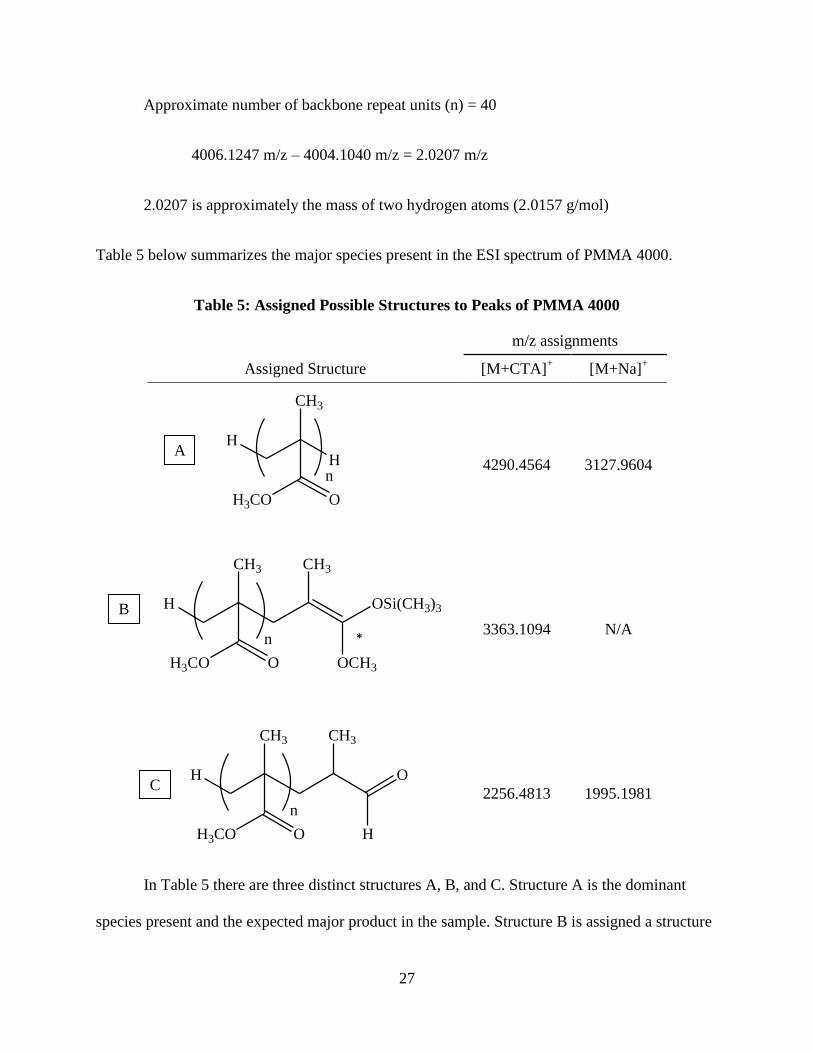
Approximate number of backbone repeat units (n) = 40
4006.1247 m/z – 4004.1040 m/z = 2.0207 m/z
2.0207 is approximately the mass of two hydrogen atoms (2.0157 g/mol)
Table 5 below summarizes the major species present in the ESI spectrum of PMMA 4000.
Table 5: Assigned Possible Structures to Peaks of PMMA 4000
m/z assignments
Assigned Structure [M+CTA]+ [M+Na]
+
4290.4564 3127.9604
3363.1094 N/A
2256.4813 1995.1981
In Table 5 there are three distinct structures A, B, and C. Structure A is the dominant
species present and the expected major product in the sample. Structure B is assigned a structure
H
CH3
OSi(CH3)3
OCH3
CH3
H3CO O
n
H
CH3
O
H
CH3
H3CO O
n
H
H
CH3
H3CO O
n
A
B
C
*
28
which would have residual trimethylsilyl still present in the sample. While structure C is
believed to be an oligomer that has been fragmented. This fragmentation was not expected
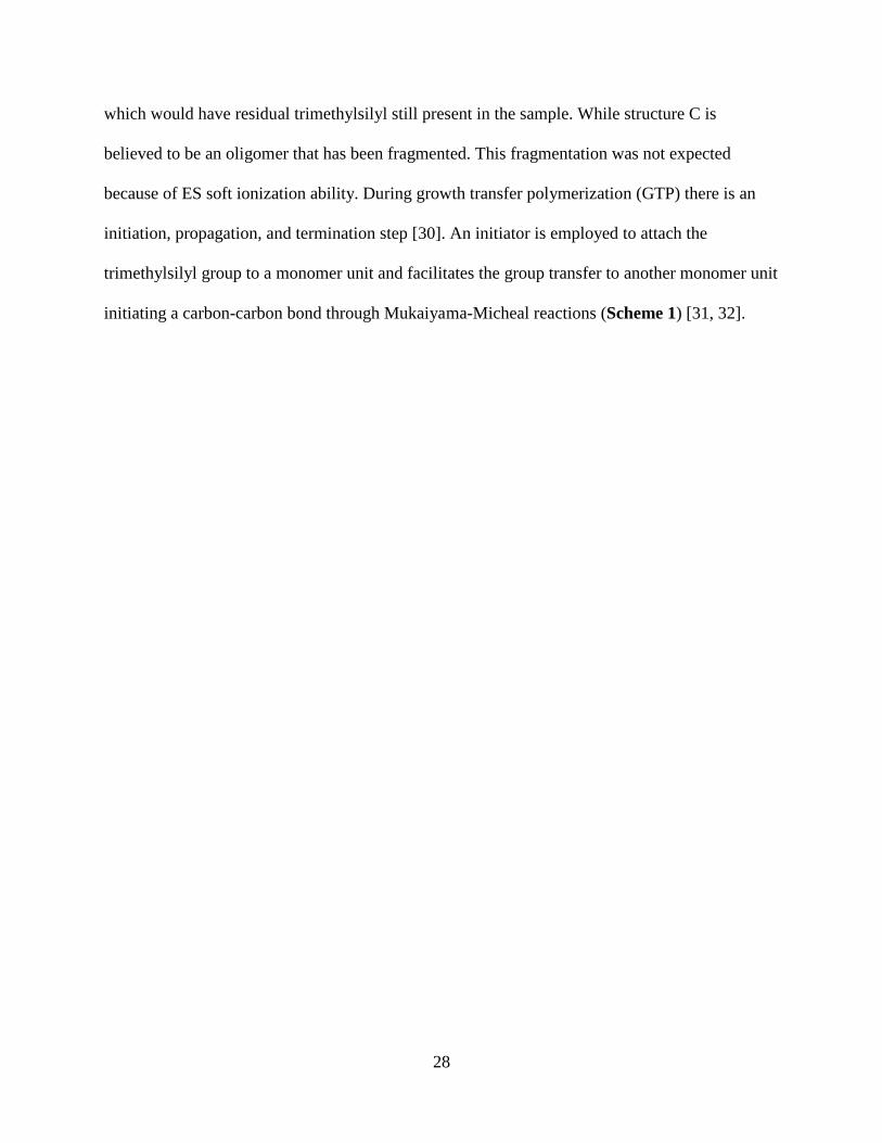
because of ES soft ionization ability. During growth transfer polymerization (GTP) there is an
initiation, propagation, and termination step [30]. An initiator is employed to attach the
trimethylsilyl group to a monomer unit and facilitates the group transfer to another monomer unit
initiating a carbon-carbon bond through Mukaiyama-Micheal reactions (Scheme 1) [31, 32].
29
Scheme 1: Group Transfer Polymerization Mechanism
O
O
SiO
O
Si
Catalyst
Catalyst
O
O
O
O
H
O
O
Si
n
OOSi
O
O
Catalyst
Initiator Si O
O
+
It is possible that not all of the trimethylsilyl was terminated and could still be present on
the end of the oligomer. The carbon-oxygen bond (*), assigned to structure B, is more labile due
to the diminished electron withdrawing nature of the oxygen by the trimethylsilyl group. This
increases the ability to stabilize the carbocation after the bond scission. It is reasonable to believe
30
that the fragmentation is occurring at this labile bond rather than the ester bond present in
assigned structure A.
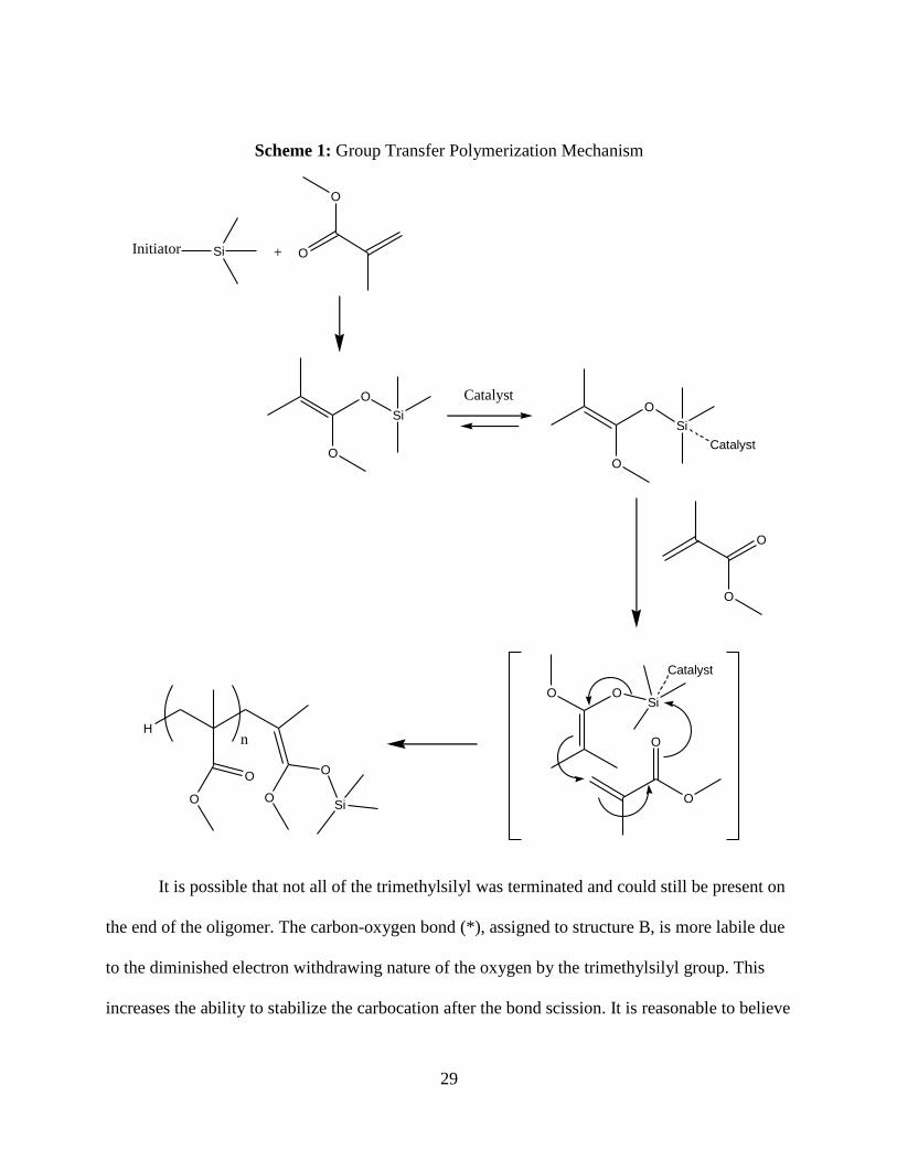
In order to further confirm that there is trimethylsilyl present in the sample we ran a
proton NMR with deuterated acetone d-6 (Figure 14). The NMR reveals a distinct peak at 0.06
ppm which would be the location of the trimethyl siloxane group.
Figure 14: NMR of PMMA 4000
2.2.2 Analysis of PMMA 8000
Achieving a clean distribution of singly charged PMMA 4000 peaks, calculating end
groups, and molecular weight distribution data was a good foundation for us to begin the analysis
of the PMMA 8000 standard. The spectrum obtained below of PMMA 8000 is under optimized
conditions without the addition of any cetyltrimethylammonium bromide (Figure 15).

31
Figure 15: ESI-ToF of PMMA 8000 without a cationizing agent at optimized parameters
While Figure 15 does have a distribution of [M + CTA]+
peaks present, it also contains a
large amount of doubly and triply charged peaks; this creates a high degree of congestion in the
lower m/z region. The high degree of congestion in this spectrum causes many lower intensity
peaks to be lost in the baseline. Once again by simply adding cetyltrimethylammonium bromide
and applying the optimized parameters we achieve a spectrum that is dominated by [M + CTA]+
peaks (Figure 16).
m/z1000 2000 3000 4000 5000 6000 7000 8000 9000 10000 11000
%
0
100

32
Figure 16: ESI-ToF of PMMA 8000 with the addition of cetyltrimethylammonium bromide under optimized conditions
There is a great improvement in the total ion intensity and [M + CTA]+ from Figure 15 to
Figure 16. It is also important to observe the peak distribution from approximately 1500 – 4000
m/z that was otherwise unobservable in Figure 15. As with PMMA 4000 the distribution of
peaks present in PMMA 8000 are out of the calibration range and required a calibration
correction. Table 6 is the mass to charge distribution of the species with the highest ion intensity
present in the spectra.
Table 6: The actual m/z, intensity, and corrected m/z of PMMA 8000
Actual m/z Intensity Corrected m/z
m/z1500 2000 2500 3000 3500 4000 4500 5000 5500 6000 6500 7000 7500 8000 8500 9000 9500 10000 10500 11000
%
0
100

33
3786.3394 7 3789.5697
7060.5718 66 7093.9298
3887.0732 7 3890.4449
7158.6260 63 7193.9035
3987.7104 7 3991.2877
7256.7622 63 7294.0451
4086.7490 6 4090.5861
7355.3721 60 7394.7571
4186.3916 6 4190.5428
7452.9805 56 7494.5340
4285.9800 8 4290.4942
7551.1987 55 7595.0245
4385.4707 7 4390.3934
7647.8760 50 7694.0284
4486.2681 8 4491.6487
7745.7559 45 7794.3566
4585.5786 9 4591.4519
7844.0933 43 7895.2493
4684.1055 11 4690.5070
7940.3237 39 7994.0746
4783.6821 11 4790.6563
8038.7891 36 8095.2932
4883.6821 10 4891.2704
8135.7378 33 8195.0510
4982.7236 12 4990.9587
8233.1807 31 8295.4171
5083.0117 15 5091.9412
8330.0869 28 8395.3307
5182.2583 16 5191.9148
8427.2529 28 8495.6141
5281.9390 19 5292.3667
8524.7606 22 8596.3539
5380.7715 21 5392.0057
8621.3428 21 8696.2413
5481.0098 24 5493.1061
8717.3691 18 8795.6574
5579.3418 28 5592.3289
8814.1387 17 8895.9489
5678.5386 30 5692.4714
8910.9443 14 8996.3853
5777.4741 34 5792.3995
9007.7813 13 9096.9632
5876.3735 43 5892.3425
9102.7256 12 9195.6827
5975.2876 45 5992.3543
9198.6904 9 9295.5727
6074.1943 49 6092.4147
9294.6016 8 9395.5185
6173.1943 52 6192.6284
9392.7490 8 9497.9119
6272.6221 56 6293.3370
9487.7734 7 9597.1623
6370.6284 60 6392.6689
9583.1211 6 9696.8661
6470.1416 61 6493.5948
9678.7402 7 9796.9725
6568.5918 64 6593.5113
9773.8955 5 9896.7140
6666.9492 65 6693.4045
9869.7207 5 9997.2821
6765.4272 65 6793.4935
9965.2939 5 10097.7132
6863.8550 65 6893.6072
10060.7432 4 10198.1445
6962.7705 63 6994.2957
10154.6200 4 10297.0519
The clean distribution of peaks from Figure 16 allows us to calculate the number average
molecular weight, weight average molecular weight, and polydispersity utilizing equations 1, 2,
34
and 3. Molecular weight distribution data from the ESI-ToF calculation, In-Lab GPC and
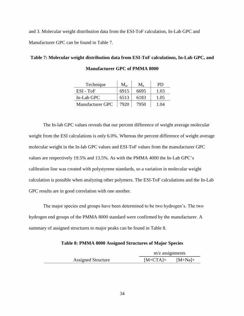
Manufacturer GPC can be found in Table 7.
Table 7: Molecular weight distribution data from ESI-ToF calculations, In-Lab GPC, and
Manufacturer GPC of PMMA 8000
Technique Mw Mn PD
ESI - ToF 6915 6695 1.03
In-Lab GPC 6513 6183 1.05
Manufacturer GPC 7920 7950 1.04
The In-lab GPC values reveals that our percent difference of weight average molecular
weight from the ESI calculations is only 6.0%. Whereas the percent difference of weight average
molecular weight in the In-lab GPC values and ESI-ToF values from the manufacturer GPC
values are respectively 19.5% and 13.5%. As with the PMMA 4000 the In-Lab GPC’s
calibration line was created with polystyrene standards, so a variation in molecular weight
calculation is possible when analyzing other polymers. The ESI-ToF calculations and the In-Lab
GPC results are in good correlation with one another.
The major species end groups have been determined to be two hydrogen’s. The two
hydrogen end groups of the PMMA 8000 standard were confirmed by the manufacturer. A
summary of assigned structures to major peaks can be found in Table 8.
Table 8: PMMA 8000 Assigned Structures of Major Species
m/z assignments
Assigned Structure [M+CTA]+ [M+Na]+
35
6293.3370 6231.2638
7168.1608 N/A
3658.7201 N/A
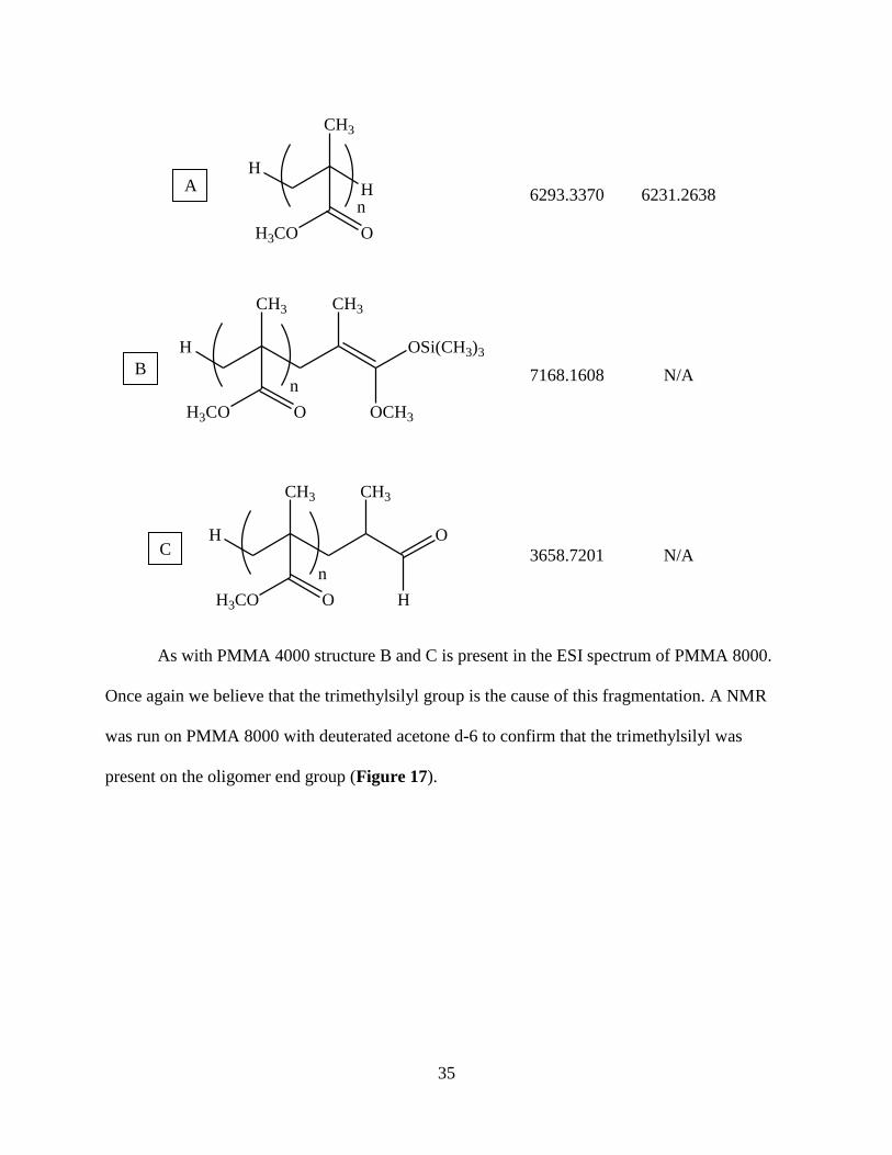
As with PMMA 4000 structure B and C is present in the ESI spectrum of PMMA 8000.
Once again we believe that the trimethylsilyl group is the cause of this fragmentation. A NMR
was run on PMMA 8000 with deuterated acetone d-6 to confirm that the trimethylsilyl was
present on the oligomer end group (Figure 17).
H
CH3
OSi(CH3)3
OCH3
CH3
H3CO O
n
H
CH3
O
H
CH3
H3CO O
n
H
H
CH3
H3CO O
n
A
B
C
36
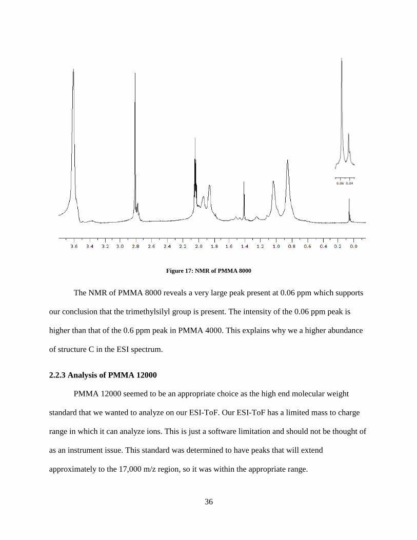
Figure 17: NMR of PMMA 8000
The NMR of PMMA 8000 reveals a very large peak present at 0.06 ppm which supports
our conclusion that the trimethylsilyl group is present. The intensity of the 0.06 ppm peak is
higher than that of the 0.6 ppm peak in PMMA 4000. This explains why we a higher abundance
of structure C in the ESI spectrum.
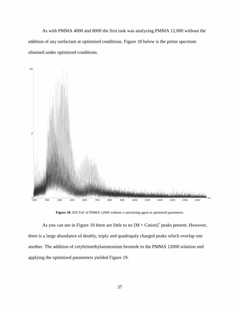
2.2.3 Analysis of PMMA 12000
PMMA 12000 seemed to be an appropriate choice as the high end molecular weight
standard that we wanted to analyze on our ESI-ToF. Our ESI-ToF has a limited mass to charge
range in which it can analyze ions. This is just a software limitation and should not be thought of
as an instrument issue. This standard was determined to have peaks that will extend
approximately to the 17,000 m/z region, so it was within the appropriate range.
37
As with PMMA 4000 and 8000 the first task was analyzing PMMA 12,000 without the
addition of any surfactant at optimized conditions. Figure 18 below is the prime spectrum
obtained under optimized conditions.
Figure 18: ESI-ToF of PMMA 12000 without a cationizing agent at optimized parameters
As you can see in Figure 18 there are little to no [M + Cation]+
peaks present. However,
there is a large abundance of doubly, triply and quadrupaly charged peaks which overlap one
another. The addition of cetyltrimethylammonium bromide to the PMMA 12000 solution and
applying the optimized parameters yielded Figure 19.
m/z2000 3000 4000 5000 6000 7000 8000 9000 10000 11000 12000 13000 14000 15000
%
0
100

38
Figure 19: ESI-ToF of PMMA 12000 with the addition of cetyltrimethylammonium bromide under optimized conditions
The first thing to observe in Figure 19 is the [M + Cation]+ region from approximately
1500 to 4000 m/z. This region was originally consumed by the triply and quadruply charged
peaks which would otherwise be unobservable previously in Figure 18. While we were able to
drastically reduce the multiply charged regions of PMMA 12000 with the addition of the
surfactant we were unable to completely rid the spectrum of the doubly charged peaks. This is
attributed to time constraints as well as issues with the ESI-ToF being unavailable. We are very
confident that with further investigation we can improve the reduction of the intensity of the
doubly charged peaks present. However the doubly charged peaks are diminished enough to be
able to calculate molecular weight distribution data. Figure 20 is just an expansion of the [M +
m/z2000 3000 4000 5000 6000 7000 8000 9000 10000 11000 12000 13000 14000 15000 16000 17000
%
0
100

39
CTA]+ region to show the clean distribution of singly charged peaks. Figures 19 and 20 have
been smoothed twice in order to reduce congestion.
Figure 20: Expansion of the [M + CTA]+ region from the ESI-ToF of PMMA 12000 with the addition of
cetyltrimethylammonium bromide under optimized conditions
As with PMMA 4000 and 8000 the distribution of peaks present in PMMA 12000 are out the
calibration range and required a calibration correction. An explanation for the ion intensity being
low is that the [M + CTA]+
species have such large masses and only one ion attached to them so
it is difficult to focus them to the mass analyzer [22]. Table 9 is the distribution of the species
with the highest ion intensity present in the spectra.
m/z10000 10500 11000 11500 12000 12500 13000 13500 14000 14500 15000 15500 16000 16500
%
0
100
40
Table 9: The actual m/z, intensity, and corrected m/z of PMMA 12000
Actual m/z Intensity Corrected m/z 10073.2734 3 10096.8808
13386.0879 13 13502.6375
10173.0986 3 10197.1250
13482.4160 13 13602.9588
10271.6924 3 10296.3185
13577.0693 12 13701.5705
10371.7588 3 10397.1873
13671.4072 12 13799.8898
10469.7402 3 10496.1464
13770.0713 12 13902.7589
10569.4805 3 10597.0777
13864.9375 11 14001.7105
10668.9746 4 10697.9553
13962.3145 11 14103.3272
10766.3818 5 10796.9037
14057.8096 11 14203.0288
10865.8936 5 10898.1764
14152.3555 9 14301.7902
10964.1865 5 10998.3884
14248.8047 10 14402.5952
11064.2451 6 11100.5776
14342.0430 9 14500.1007
11162.9160 6 11201.5174
14440.0346 8 14602.6399
11259.3652 5 11300.3379
14534.7988 7 14701.8662
11358.3799 5 11401.9366
14633.0400 7 14804.8024
11455.7588 5 11501.9964
14725.1797 6 14901.4113
11547.8457 5 11596.7379
14822.9220 6 15003.9654
11647.8701 5 11699.7686
14918.7314 6 15104.5626
11744.1172 6 11799.0208
15011.6279 5 15202.1680
11840.0557 6 11898.0560
15106.7266 6 15302.1537
11938.2744 7 11999.5415
15204.9063 5 15405.4461
12034.5693 7 12099.1259
15297.5605 4 15502.9837
12131.6367 8 12199.5886
15392.4814 4 15602.9606
12228.6406 8 12300.0580
15490.1494 4 15705.8788
12320.0410 9 12394.7839
15584.2793 3 15805.1048
12417.6719 9 12496.0257
15673.8467 3 15899.5437
12519.3125 11 12601.4837
15775.1787 3 16006.3980
12612.2764 11 12697.9865
15868.7197 3 16105.0299
12712.5469 11 12802.1202
15965.8486 3 16207.4176
12808.2441 12 12901.5454
16057.3701 2 16303.8472
12905.1728 12 13002.2881
16151.8838 2 16403.3564
13003.4092 12 13104.4267
16248.9385 2 16505.4335
13096.5029 12 13201.2508
16345.7510 2 16607.1125
13194.5117 12 13303.2205
16437.5430 2 16703.3507
13287.3398 14 13399.8315

41
The distribution of peaks from Figure 20 allows us to calculate the number average
molecular weight, weight average molecular weight, and polydispersity utilizing equations 1, 2,
and 3. Molecular weight distribution data from the ESI-ToF calculation, In-Lab GPC and
Manufacturer GPC can be found in Table 10.
Table 10: Molecular weight distribution data from ESI-ToF calculations, In-Lab GPC, and
Manufacturer GPC of PMMA 12000
Technique Mw Mn PD
ESI - ToF 13150 12982 1.01
In-Lab GPC 12692 11987 1.06
Manufacturer GPC 12000 11540 1.04
The In-Lab GPC values reveals that our percent difference of weight average molecular
weight from the ESI calculations is only 3.5%. Whereas the percent difference of weight average
molecular weight in the GPC values and ESI values from the manufacturer values are
respectively 5.6% and 9.1%. Further investigation of the PMMA 12000 is needed to fully
elucidate the standard but current results seem very promising. The low ion abundance present
could prove to be an issue with the molecular weight distribution calculations, but our
calculations still seem to be in good correlation with one another. As with the PMMA 4000 and
8000 the In-Lab GPC’s calibration line was created with polystyrene standards, so a variation in
molecular weight calculation is possible when analyzing other polymers.
Table 11 is the assigned structures of the major species present in the ESI spectrum of
PMMA 12000.

42
Table 11: PMMA 12000 Assigned Structures of Major Species
m/z assignments
Assigned Structure [M+CTA]+ [M+Na]+
13399.8315 11637.8448
10470.4359 N/A
3057.1060 2796.0105
H
CH3
OSi(CH3)3
OCH3
CH3
H3CO O
n
H
CH3
O
H
CH3
H3CO O
n
H
H
CH3
H3CO O
nA
B
C
43
As with PMMA 4000 and 8000 we have come to the same conclusion with PMMA
12000 that structure C is a result of the fragmentation of the labile bond in structure B. The NMR
of PMMA 12000 did not reveal trimethylsilyl group. However, this is not a surprise because as
the molecular weight of the polymer grows the backbone concentration increases and the end
group’s concentration decreases. The concentration the trimethylsilyl end group appears to be so
low that it is unobservable by NMR.
2.3 Surfactant Consideration
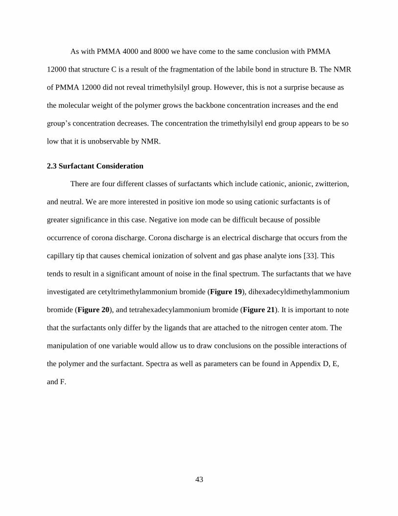
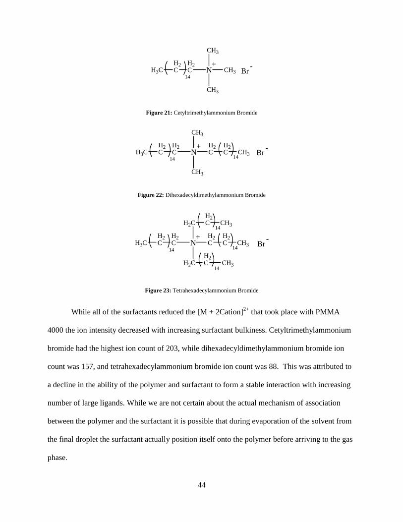
There are four different classes of surfactants which include cationic, anionic, zwitterion,
and neutral. We are more interested in positive ion mode so using cationic surfactants is of
greater significance in this case. Negative ion mode can be difficult because of possible
occurrence of corona discharge. Corona discharge is an electrical discharge that occurs from the
capillary tip that causes chemical ionization of solvent and gas phase analyte ions [33]. This
tends to result in a significant amount of noise in the final spectrum. The surfactants that we have
investigated are cetyltrimethylammonium bromide (Figure 19), dihexadecyldimethylammonium
bromide (Figure 20), and tetrahexadecylammonium bromide (Figure 21). It is important to note
that the surfactants only differ by the ligands that are attached to the nitrogen center atom. The
manipulation of one variable would allow us to draw conclusions on the possible interactions of
the polymer and the surfactant. Spectra as well as parameters can be found in Appendix D, E,
and F.
44
N
CH3
H2C CH3
CH3
H2CH3C
14
+Br
-
Figure 21: Cetyltrimethylammonium Bromide
N
CH3
H2C
H2C
CH3
H2CH3C
14
H2C CH3
14
+Br
-
Figure 22: Dihexadecyldimethylammonium Bromide
N
H2C
H2C
H2C
H2C
H2CH3C
14
H2C
H2C
H2C
CH3
CH3
CH3
14
14
14
+Br
-
Figure 23: Tetrahexadecylammonium Bromide
While all of the surfactants reduced the [M + 2Cation]2+
that took place with PMMA
4000 the ion intensity decreased with increasing surfactant bulkiness. Cetyltrimethylammonium
bromide had the highest ion count of 203, while dihexadecyldimethylammonium bromide ion
count was 157, and tetrahexadecylammonium bromide ion count was 88. This was attributed to
a decline in the ability of the polymer and surfactant to form a stable interaction with increasing
number of large ligands. While we are not certain about the actual mechanism of association
between the polymer and the surfactant it is possible that during evaporation of the solvent from
the final droplet the surfactant actually position itself onto the polymer before arriving to the gas
phase.

45
2.4 Conclusion and Suggestions for Future Work
In conclusion this will be the first report detailing successful use of ESI-ToF to produce
clean mass spectral data for PMMA with molecular weights > 3,000 g/mol. This was
accomplished by utilizing cetyltrimethylammonium bromide and adjusting critical ESI
parameters. We hypothesize that the parent and offspring droplets will have less cationizing
agent because cetyltrimethylammonium ion is a great deal larger than other typical cationizing
agents (i.e. Na+) so less charge will be able to exist on the exterior of the droplet. The large
surface area of the cetyltrimethylammonium ion will also hinder the polymers ability to gain
multiple charges. The molecular weight data is in good agreement with In-lab GPC-MALS from
1,000 – 13,000 m/z (g/mol) with a percent difference of 6.6% for PMMA 4000, 6.0% for PMMA
8000, and 3.5% for PMMA 12000.
One of the long term goals of this project is to incorporate chromatographic separation,
such as GPC. Addition of GPC would allow separation of highly complex mixtures prior to ESI-
MS analysis. Also we could evaluate other surfactants and solvent systems. By creating a two
part solvent system in which the core of the droplet is insoluble with the analyte and the outside
of the solvent layer holds onto the analyte the offspring droplets will have predominately analyte
present. Upon solvent evaporation from the final droplet more analyte will be ejected to the gas
phase. A fluorinated surfactant could be of interest in analyzing a fluoropolymer. Typically
fluropolymer’s are not soluble in conventional ESI solvents; however the addition of a
fluorinated surfactant may be able to bridge this gap by acting as a phase interface transferring
agent. As stated earlier our ESI-ToF mass to charge range only extends to 20,000 m/z so using a
surfactant with a higher charge state (i.e. +2, +3) could possibly control the charge state
distribution. Controlling the charge state distribution could prove to be a valuable tool when

46
analyzing polymers which molecular weights which exceed the ESI-ToF mass to charge range.
Finally we plan on expanding this application to other synthetic polymers

CHAPTER 3: EXPERIMENTAL
3.1 Materials
The LC/UV grade acetone was manufactured by ChromAR (Lot number H14B00) and
used without further alteration. The HPLC grade solvent tetrahydrofuran (THF) (Lot number
G35804) was manufactured by J.T. Baker and used without further alteration. Anhydrous toluene
(99.8%) was manufactured from Sigma Aldrich and used without further alteration.
Poly (methyl methacrylate) (PMMA) 4000 (Lot number WA22833) and 8000 (Lot
number 0001428483) were purchased from Sigma Aldrich and were manufactured by Fluka
utilizing group transfer polymerization. PMMA 12000 (Lot number 510978) was manufactured
by Polymer Sciences Incorporated utilizing group transfer polymerization. Varian Incorporated
polystyrene standards kit (Lot number 101) was manufactured by Polymer Labs and used
without further alteration.
Cetyltrimethylammonium bromide (CTAB) (Lot number 116464641505047) was
manufactured by Sigma and used without further alteration. Dihexadecyldimethylammonium
bromide (Lot number 13813LH) and Tetrahexadecylammonium bromide (Lot number
04757811) were manufactured from Aldrich and were used without further alteration.
3.2 GPC Polystyrene Sample Preparation and Calibration
The following groups of polystyrene (PS) standards from Polymer Labs were added to
three different 20 mL scintillation vials in preparation of GPC calibration. Vial one contained
0.0153 grams of PS 640, 0.0136 grams of PS 10290, 0.0113 grams of PS 200100, and 0.0051
grams of PS 2748000. Vial two contained 0.0158 grams of PS 1490, 0.0148 grams of PS 29460,
and 0.0092 grams of PS 458700. Vial three contained 0.0148 grams of PS 3950, 0.0118 grams of
48
PS 69200, and 0.0061 grams of PS 1202000. Exactly 10.00 mL of THF was pipette into each
scintillation vial. The solutions were allowed to sit for approximately one day before analysis.
The columns were set in the following order: PLgel Mixed-C, PLgel Mixed-E, Waters HR 2, and
Waters HR 0.5. Distribution data was extracted from Millennium and imported to Cirrus in order
to create the calibration curve.
3.2.1 PMMA Standard Sample Preparation and Analysis for GPC
0.0051 grams of PMMA 4000 was added to a 20 mL scintillation vial followed by 1.5
mL of THF. The sample was then spiked with 2 µM of toluene. 0.0047 grams of PMMA 8000
was added to a 20 mL scintillation vial followed by 1.5 mL of THF. The sample was then spiked
with 2 µM of toluene. 0.0051 grams of PMMA 12000 was added to a 20 mL scintillation vial
followed by 1.5 mL of THF. The sample was then spiked with 2 µM of toluene. The solutions
were allowed to sit for approximately one day before analysis. Distribution data was extracted
from Millennium and imported to Cirrus. Molecular weight data from each run was calculated
using the calibration line created from the PS standards.
3.3 ESI-ToF Sample Preparation
0.0041 g of the Sigma cetyltrimethylammonium bromide (CTAB) surfactant was added
to a 20 mL scintillation vial followed by 20.00 mL of LC/UV grade acetone. The solution was
stored in a lab drawer until necessary for ESI-ToF analysis.
0.0109 g of the Fluka PMMA 4000 standard was added to a 20 mL scintillation vial
followed by the addition of 20.00 mL of LC/UV grade acetone. The standard was stored in a lab
drawer until ESI-ToF analysis. Prior to ESI analysis 40.0 µL of the solution was transferred to a

49
20 mL scintillation vial followed by the addition 70.0 µL of the CTAB solution. 10.00 mL of the
LC/UV grade acetone was then added to the scintillation vial.
0.0202 g of the Fluka PMMA 8000 standard was added to a 20 mL scintillation vial
followed by the addition of 20.00 mL of LC/UV grade acetone. The standard was stored in a lab
drawer until ESI-ToF analysis. Prior to ESI analysis 150.0 µL of the solution was transferred to a
20 mL scintillation vial followed by the addition of 40.0 µL of the CTAB solution. 10.00 mL of
the LC/UV grade acetone was then added to the scintillation vial.
0.0255 g of the Polymer Sciences PMMA 12000 standard was added to a 20 mL
scintillation vial followed by the addition of 20.00 mL of LC/UV grade acetone. The standard
was stored in a lab drawer until ESI-ToF analysis. Prior to ESI analysis 50.0 µL of the solution
was transferred to a 20 mL scintillation vial followed by the addition of 30.0 µL of the CTAB
solution. 10.00 mL of the LC/UV grade acetone was then added to the scintillation vial.
0.0044 g of the Aldrich dihexadecyldimethylammonium bromide surfactant was added to
a 20 mL scintillation vial followed by 20.00 mL of LC/UV grade acetone. The solution was
stored in a lab drawer until necessary ESI-ToF analysis. Prior to ESI analysis 45.0 µL of the
PMMA solution was transferred to a 20 mL scintillation vial followed by the addition of 26.6 µL
of the dihexadecyldimethylammonium bromide solution. 10.00 mL of the LC/UV grade acetone
was then added to the scintillation vial.
0.0045 g of the Sigma tetrahexadecylammonium bromide surfactant was added to a 20
mL scintillation vial followed by 20.00 mL of LC/UV grade acetone. The solution was stored in
a lab drawer until necessary ESI-ToF analysis. Prior to ESI analysis 45.0 µL of the PMMA
solution was transferred to a 20 mL scintillation vial followed by the addition of 26.6 µL of the

50
tetrahexadecylammonium bromide solution. 10.00 mL of the LC/UV grade acetone was then
added to the scintillation vial.
3.3.2 ESI Parameters for Each Sample
PMMA 4000 spectrum without CTAB (Figure 11) had the following ES parameters applied:
Parameter Setting
Capillary Voltage 2900
Sample Cone Voltage 100
Extraction Cone Voltage 2.0
Source Temperature (°C) 90
Desolvation Temperature (°C) 150
Cone Gas Flow Rate (L/hr) 0
Desolvation Gas Flow Rate (L/hr) 500
Syringe Pump Flow Rate (µL/min) 5.0
Analysis Time – 5 minutes
PMMA 4000 with CTAB (Figure 12) had the following ES parameters applied:
Parameter Setting
Capillary Voltage 2900
Sample Cone Voltage 100
Extraction Cone Voltage 2.0
Source Temperature (°C) 90
Desolvation Temperature (°C) 150
Cone Gas Flow Rate (L/hr) 0
Desolvation Gas Flow Rate (L/hr) 500
Syringe Pump Flow Rate (µL/min) 5.0
Analysis Time – 5 minutes
PMMA 8000 without CTAB (Figure 14) had the following ES parameters applied:
Parameter Setting
Capillary Voltage 2900
Sample Cone Voltage 140
Extraction Cone Voltage 2.0
Source Temperature (°C) 90

51
Desolvation Temperature (°C) 150
Cone Gas Flow Rate (L/hr) 0
Desolvation Gas Flow Rate (L/hr) 500
Syringe Pump Flow Rate (µL/min) 10.0
Analysis Time – 6 minutes
Smoothing
Smooth window (channels) – 3
Number of smooths – 2
PMMA 8000 with CTAB (Figure 15) had the following ES parameters applied:
Parameter Setting
Capillary Voltage 2900
Sample Cone Voltage 140
Extraction Cone Voltage 2.0
Source Temperature (°C) 90
Desolvation Temperature (°C) 140
Cone Gas Flow Rate (L/hr) 0
Desolvation Gas Flow Rate (L/hr) 500
Syringe Pump Flow Rate (µL/min) 10.0
Analysis Time – 6 minutes
Smoothing
Smooth window (channels) – 3
Number of smooths – 2
PMMA 12000 without CTAB (Figure 16) had the following ES parameters applied:
Parameter Setting
Capillary Voltage 2900
Sample Cone Voltage 150
Extraction Cone Voltage 2.0
Source Temperature (°C) 90
Desolvation Temperature (°C) 150
Cone Gas Flow Rate (L/hr) 0
Desolvation Gas Flow Rate (L/hr) 500
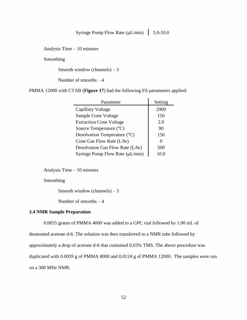
52
Syringe Pump Flow Rate (µL/min) 5.0-10.0
Analysis Time – 10 minutes
Smoothing
Smooth window (channels) – 3
Number of smooths – 4
PMMA 12000 with CTAB (Figure 17) had the following ES parameters applied:
Parameter Setting
Capillary Voltage 2900
Sample Cone Voltage 150
Extraction Cone Voltage 2.0
Source Temperature (°C) 90
Desolvation Temperature (°C) 150
Cone Gas Flow Rate (L/hr) 0
Desolvation Gas Flow Rate (L/hr) 500
Syringe Pump Flow Rate (µL/min) 10.0
Analysis Time – 10 minutes
Smoothing
Smooth window (channels) – 3
Number of smooths – 4
3.4 NMR Sample Preparation
0.0055 grams of PMMA 4000 was added to a GPC vial followed by 1.00 mL of
deuterated acetone d-6. The solution was then transferred to a NMR tube followed by
approximately a drop of acetone d-6 that contained 0.03% TMS. The above procedure was
duplicated with 0.0059 g of PMMA 8000 and 0.0124 g of PMMA 12000. The samples were run
on a 300 MHz NMR.

REFERENCES
1. Flory, P.J., Principles of Polymer Chemistry 1953, Ithaca, N.Y.: Cornell University
Press.
2. Goodyear, C., Improvement In India-Rubber Fabrics. 1844.
3. Baekeland, L.H., Synthesis of condensation product of phenols and formaldehyde. 1908.
4. Staudinger, H., Polymerization. Berichte der Deutschen Chemischen Gesellschaft
[Abteilung] B: Abhandlungen, 1920. 53B: p. 1073-1085.
5. Jiang, X., et al., Mass Spectrometric Characterization of Functional Poly(methyl
methacrylate) in Combination with Critical Liquid Chromatography Analytical
Chemistry, 2003. 75(20): p. 5517-5524.
6. Jackson, A.T., et al., Characterization of end groups in poly(2-hydroxyethyl
methacrylate) by means of electrospray ionization-mass spectrometry/mass spectrometry
(ESI-MS/MS) Polymer, 2010. 51(6): p. 1418-1424.
7. Romack, T.J., et al., Characterization of perfluoroalkyl acrylic oligomers by
electrospray ionization time-of-flight mass spectrometry Rapid Communications in Mass
Spectrometry, 2008. 22(7): p. 930-934.
8. Murgasova, R. and D.M. Hercules, Polymer characterization by combining liquid
chromatography with MALDI and ESI mass spectrometry Analytical and Bioanalytical
Chemistry, 2002. 373(6): p. 481-489.
9. Dole, M., et al., Molecular beams of macroions. Journal of Chemical Physics, 1968.
49(5): p. 2240-2249.
10. Fenn, J.B. and M. Yamashita, Electrospray ion source. Another variation on the free-jet
theme Journal of Physical Chemistry, 1984. 88(20): p. 4451-4459.
11. Tanaka, K., et al., Protein and polymer analyses up to m/z 100,000 by laser ionization
time-of-flight mass spectrometry Rapid Communications in Mass Spectrometry, 1988.
2(8): p. 151-153.
12. Crews, P., J. Rodriguez, and M. Jaspars, Organic Structure Analysis. Topics In Organic
Chemistry, ed. K. Houk. 1998, New York: Oxford University Press.
13. Iribarne, J.V. and B.A. Thomson, On the evaporation of small ions from charged
droplets. Journal of Chemical Physics, 1976. 64(6): p. 2287-2294.
14. Kebarle, P., A brief overview of the present status of the mechanisms involved in
electrospray mass spectrometry. Journal of Mass Spectrometry, 2000. 35: p. 804-817.
54
15. Rayleigh, L., Philos. Mag., 1882. 49: p. 2240.
16. Cole, R.B. and G. Wang, Effects of solvent and counterion on ion pairing and observed
charge states of diquaternary ammonium salts in electrospray ionization mass
spectrometry Journal of the American Society for Mass Spectrometry, 1996. 7(10): p.
1050-1058.
17. Iavarone, A.T. and E.R. Williams, Mechanism of Charging and Supercharging Molecules
in Electrospray Ionization Journal of the American Chemical Society, 2003. 125(8): p.
2319-2327.
18. Sherman, C.L. and J.S. Brodbelt, An equilibrium partitioning model for predicting
response to host-guest complexation in electrospray ionization mass spectrometry
Analytical chemistry, 2003. 75(8): p. 1828-1836.
19. Cech, N.B. and C.G. Enke, Relating Electrospray Ionization Response to Nonpolar
Character of Small Peptides. Analytical Chemistry, 2000. 72(13): p. 2717-2723.
20. Tang, K. and R.D. Smith, Physical/chemical separations in the break-up of highly
charged droplets from electrosprays Journal of the American Society for Mass
Spectrometry, 2001. 12(3): p. 343-347.
21. Grimm, R.L. and J.L. Beauchamp, Evaporation and Discharge Dynamics of Highly
Charged Droplets of Heptane, Octane, and p-Xylene Generated by Electrospray
Ionization. Analytical Chemistry, 2002. 74(24): p. 6291-6297.
22. Hunt, S.M., et al., Probing the Effects of Cone Potential in the Electrospray Ion Source:
Consequences for the Determination of Molecular Weight Distributions of Synthetic
Polymers Analytical Chemistry, 1998. 70(9): p. 1812-1822.
23. Kehr, S. and H. Luftmann, Polymer characterization by electrospray-mass-spectrometry
- shifting the upper mass limit e-Polymers, 2007.
24. Touboul, D., M.C. Jecklin, and R. Zenobi, Ion internal energy distributions validate the
charge residue model for small molecule ion formation by spray methods Rapid
Communications in Mass Spectrometry, 2008. 22(7): p. 1062-1068.
25. Fenn, J.B., Ion formation from charged droplets: roles of geometry, energy, and time
Journal of the American Society for Mass Spectrometry, 1993. 4(7): p. 524-535.
26. Fenn, J.B. and T. Nohmi, Electrospray mass spectrometry of poly(ethylene glycols) with
molecular weights up to five million. Journal of the American Chemical Society, 1992.
114(9): p. 3241-3246.
55
27. Enke, C.G., A predictive model for matrix and analyte effects in electrospray ionization
of singly-charged ionic analytes Analytical Chemistry, 1997. 69(23): p. 4885-4893.
28. Waters, Micromass Q-Tof micro Mass Spectrometer Operator’s Guide. 2002.
29. Bahadur, P. and N.V. Sastry, Principles of Polymer Science. 2002, New Dehli: Narosa
Publishing House.
30. Webster, O.W., et al., Group-transfer polymerization. 1. A new concept for addition
polymerization with organosilicon initiators Journal of the American Chemical Society,
1983. 105(17): p. 5706-5708.
31. Raynaud, J., Y. Gnanou, and D. Taton, Group Transfer Polymerization of (Meth)acrylic
Monomers Catalyzed by N-Heterocyclic Carbenes and Synthesis of All Acrylic Block
Copolymers: Evidence for an Associative Mechanism Macromolecules, 2009. 42(16): p.
5996-6005.
32. Scholten, M.D., J.L. Hedrick, and R.M. Waymouth, Group Transfer Polymerization of
Acrylates Catalyzed by N-Heterocyclic Carbenes. Macromolecules, 2008. 41(20): p.
7399-7404.
33. Kebarle, P. and H. Yeunghaw, eds. On the mechanism of electrospray mass
spectrometry. Electrospray Ionization Mass Spectrometry, ed. R.B. Cole. 1997, Wiley:
New York. 3-63.

APPENDIX A. Calibration of PMMA 4000.
Calculated ESI Peaks of PMMA 4000 with two hydrogen end groups with CTAB as the
cationizing agent
n m/z
1 386.3998
10 1286.8717
20 2288.3994
30 3289.9270
40 4290.4512
50 5291.9790
60 6293.5063
70 7294.0308
80 8295.5586
90 9296.0830
100 10297.6104
Actual Collected ESI Data of PMMA 4000
n m/z
10 1387.0931
11 1487.1329
12 1588.1923
13 1688.2686
14 1788.3169
15 1888.3674
16 1988.3804
17 2088.4080
18 2188.4202
19 2288.4287
20 2388.3948
21 2488.3406
22 2588.2805
23 2688.1929
24 2788.0654
25 2887.8955
26 2987.4190
27 3087.5149
28 3187.2622
29 3286.9307
57
30 3387.6172
31 3487.1968
32 3586.7632
33 3686.2539
34 3785.6951
35 3885.0593
36 3984.3513
37 4083.6096
38 4182.7554
39 4281.8633
40 4380.8257
41 4479.7881
42 4579.5825
43 4678.3066
44 4775.9565
45 4875.5557
46 4974.0425
47 5072.1992
48 5169.6133
49 5268.5703
50 5366.6226
51 5464.6636
52 5561.9966
53 5659.5723
54 5756.2295
55 5854.2622
56 5952.5537
57 6049.7388
58 6145.5884
59 6243.1260
60 6339.5972
61 6437.2598
62 6532.5767
63 6628.0586

58
Linear trendline of the calculated ESI data – y = 9.98854E-03xc - 2.85816
6th
order polynomial trendline of the actual ESI data – y = 1.15827E-22xa6 - 2.90130E-18xa
5 +
2.92418E-14xa4 - 1.44442E-10xa
3 + 3.77375E-07xa
2 + 9.49660E-03xa - 2.61286
Equations set equal and solved for xc -
xc = (1.15827E-22xa6 - 2.90130E-18xa
5 + 2.92418E-14xa
4 - 1.44442E-10xa
3 + 3.77375E-07xa
2 +
9.49660E-03xa + 0.24530) / 9.98854E-03
y = 9.98854E-03x - 2.85816
R² = 1.00000
y = 1.15827E-22x6 - 2.90130E-18x5 + 2.92418E-14x4 - 1.44442E-
10x3 + 3.77374E-07x2 + 9.49660E-03x - 2.61286
R² = 1.000000
20
40
60
80
100
120
0 2000 4000 6000 8000 10000 12000
Nu
mb
er o
f b
ack
bo
ne
rep
eat
un
its
(n)
Peak mass to charge ratio (m/z)
Corrected Data
ESI Data
Linear (Corrected Data)
Poly. (ESI Data)

APPENDIX B. Calibration of PMMA 8000.
Calculated ESI Peaks of PMMA 8000 with two hydrogen end groups with CTAB as the
cationizing agent
n m/z
1 386.3998
10 1286.8717
20 2288.3994
30 3289.9270
40 4290.4512
50 5291.9790
60 6293.5063
70 7294.0308
80 8295.5586
90 9296.0830
100 10297.6104
Actual Collected ESI Data of PMMA 8000
n m/z
10 1387.0931
11 1487.1329
12 1588.1923
13 1688.2686
14 1788.3169
15 1888.3674
16 1988.3804
17 2088.4080
18 2188.4202
19 2288.4287
20 2388.3948
21 2488.3406
22 2588.2805
23 2688.1929
24 2788.0654
25 2887.8955
26 2987.4190
27 3087.5149
28 3187.2622
29 3286.9307

60
30 3387.6172
31 3487.1968
32 3586.7632
33 3686.2539
34 3785.6951
35 3885.0593
36 3984.3513
37 4083.6096
38 4182.7554
39 4281.8633
40 4380.8257
41 4479.7881
42 4579.5825
43 4678.3066
44 4775.9565
45 4875.5557
46 4974.0425
47 5072.1992
48 5169.6133
49 5268.5703
50 5366.6226
51 5464.6636
52 5561.9966
53 5659.5723
54 5756.2295
55 5854.2622
56 5952.5537
57 6049.7388
58 6145.5884
59 6243.1260
60 6339.5972
61 6437.2598
62 6532.5767
63 6628.0586
61
Linear trendline of the calculated data – y = 9.98854E-03xc - 2.85816
6th
order polynomial trendline of the actual ESI data – y = 2.13185E-23xa6 - 9.45430E-19xa
5 +
1.70983E-14xa4 - 1.57815E-10xa
3 + 8.04178E-07xa
2 + 7.85639E-03xa - 5.56546E-01
Equations set equal and solved for xc -
xc = (2.13185E-23xa6 - 9.45430E-19xa
5 + 1.70983E-14xa
4 - 1.57815E-10xa
3 + 8.04178E-07xa
2 +
7.85639E-03xa + 2.3016) / 9.98854E-03
y = 9.98854E-03x - 2.85816
R² = 1.00000
y = 2.13185E-23x6 - 9.45430E-19x5 + 1.70983E-14x4 -
1.57815E-10x3 + 8.04178E-07x2 + 7.85639E-03x - 5.56546E-01
R² = 1.000000
20
40
60
80
100
120
0 2000 4000 6000 8000 10000 12000
Nu
mb
er o
f b
ack
bo
ne
rep
eat
un
tis
(n)
Peak mass to charge ratio (m/z)
Calibrated Data
Series2
Linear (Calibrated Data)
Poly. (Series2)
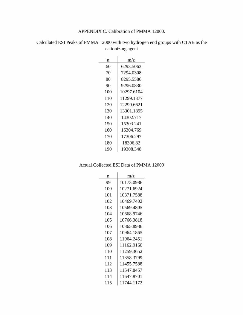
APPENDIX C. Calibration of PMMA 12000.
Calculated ESI Peaks of PMMA 12000 with two hydrogen end groups with CTAB as the
cationizing agent
n m/z
60 6293.5063
70 7294.0308
80 8295.5586
90 9296.0830
100 10297.6104
110 11299.1377
120 12299.6621
130 13301.1895
140 14302.717
150 15303.241
160 16304.769
170 17306.297
180 18306.82
190 19308.348
Actual Collected ESI Data of PMMA 12000
n m/z
99 10173.0986
100 10271.6924
101 10371.7588
102 10469.7402
103 10569.4805
104 10668.9746
105 10766.3818
106 10865.8936
107 10964.1865
108 11064.2451
109 11162.9160
110 11259.3652
111 11358.3799
112 11455.7588
113 11547.8457
114 11647.8701
115 11744.1172
63
116 11840.0557
117 11938.2744
118 12034.5693
119 12131.6367
120 12228.6406
121 12320.0410
122 12417.6719
123 12519.3125
124 12612.2764
125 12712.5469
126 12808.2441
127 12905.1728
128 13003.4092
129 13096.5029
130 13194.5117
131 13287.3398
132 13386.0879
133 13482.4160
134 13577.0693
135 13671.4072
136 13770.0713
137 13864.9375
138 13962.3145
139 14057.8096
140 14152.3555
141 14248.8047
142 14342.0430
143 14440.0346
144 14534.7988
145 14633.0400
146 14725.1797
147 14822.9220
148 14918.7314
149 15011.6279
150 15106.7266
151 15204.9063
152 15297.5605
153 15392.4814
154 15490.1494
155 15584.2793
156 15673.8467
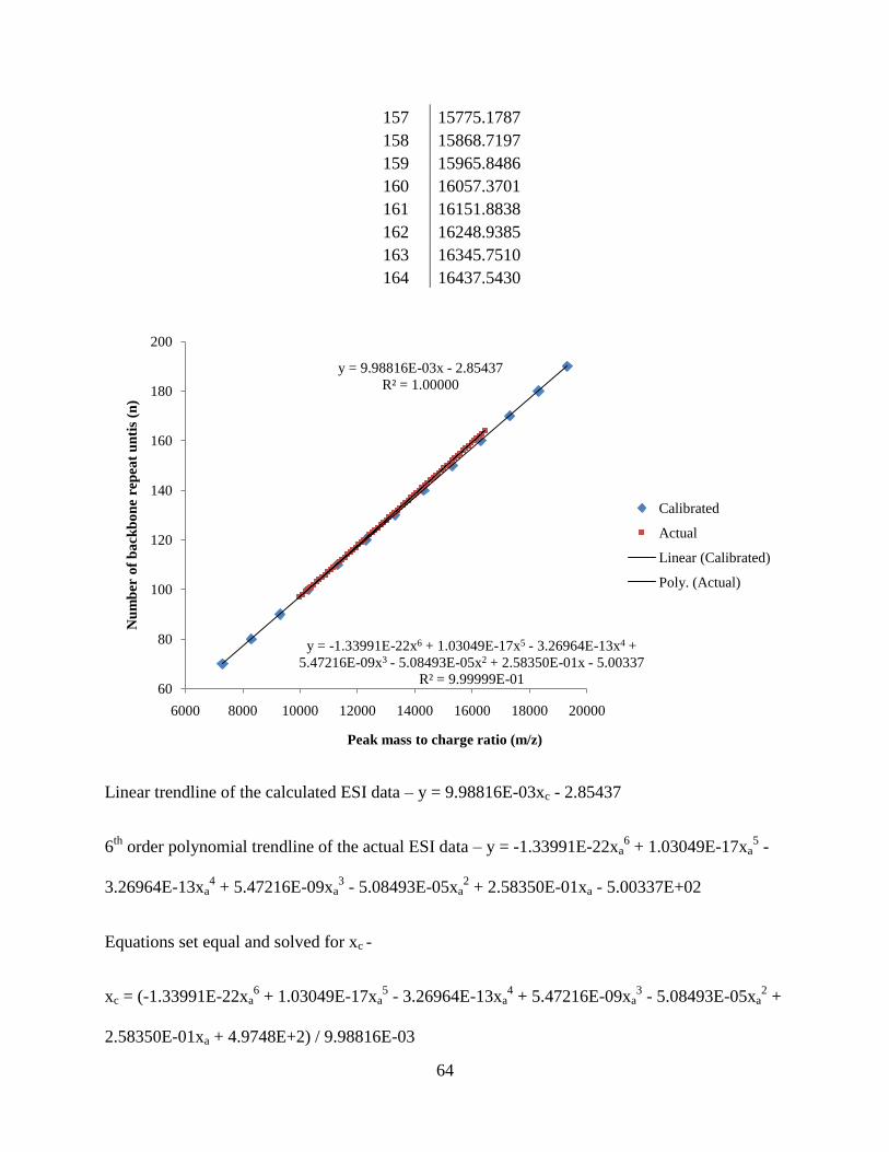
64
157 15775.1787
158 15868.7197
159 15965.8486
160 16057.3701
161 16151.8838
162 16248.9385
163 16345.7510
164 16437.5430
Linear trendline of the calculated ESI data – y = 9.98816E-03xc - 2.85437
6th
order polynomial trendline of the actual ESI data – y = -1.33991E-22xa6 + 1.03049E-17xa
5 -
3.26964E-13xa4 + 5.47216E-09xa
3 - 5.08493E-05xa
2 + 2.58350E-01xa - 5.00337E+02
Equations set equal and solved for xc -
xc = (-1.33991E-22xa6 + 1.03049E-17xa
5 - 3.26964E-13xa
4 + 5.47216E-09xa
3 - 5.08493E-05xa
2 +
2.58350E-01xa + 4.9748E+2) / 9.98816E-03
y = 9.98816E-03x - 2.85437
R² = 1.00000
y = -1.33991E-22x6 + 1.03049E-17x5 - 3.26964E-13x4 +
5.47216E-09x3 - 5.08493E-05x2 + 2.58350E-01x - 5.00337
R² = 9.99999E-0160
80
100
120
140
160
180
200
6000 8000 10000 12000 14000 16000 18000 20000
Nu
mb
er o
f b
ack
bo
ne
rep
eat
un
tis
(n)
Peak mass to charge ratio (m/z)
Calibrated
Actual
Linear (Calibrated)
Poly. (Actual)
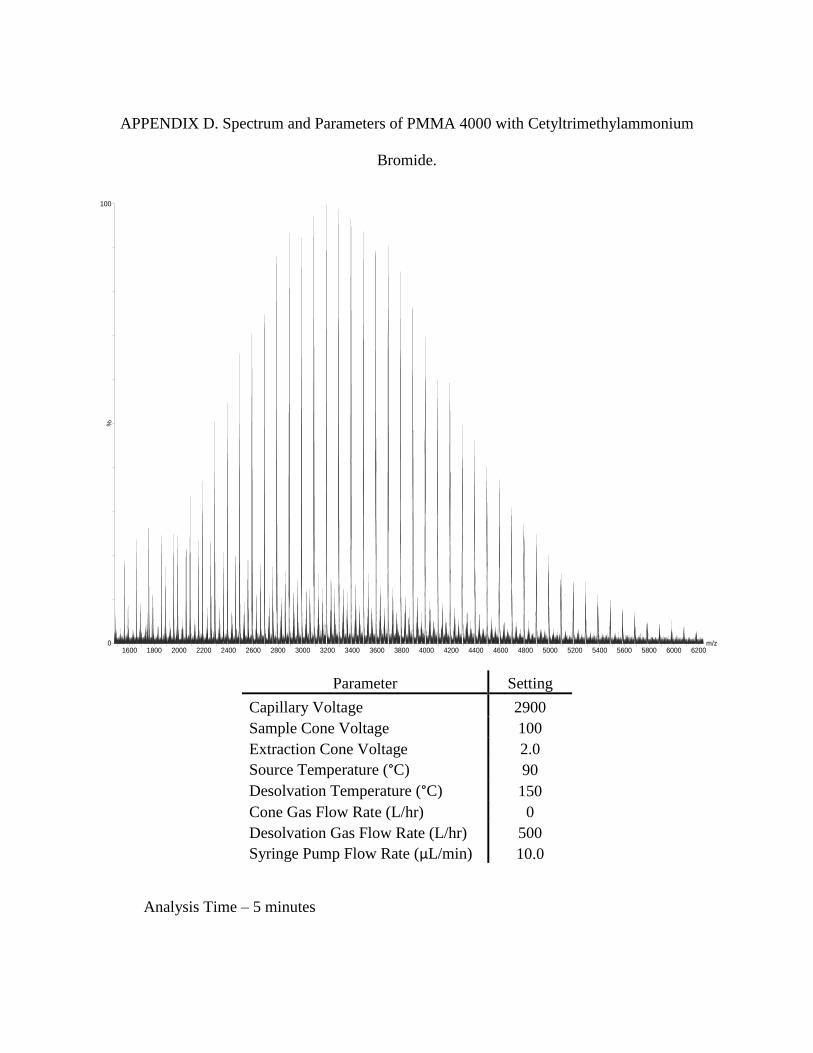
APPENDIX D. Spectrum and Parameters of PMMA 4000 with Cetyltrimethylammonium
Bromide.
Parameter Setting
Capillary Voltage 2900
Sample Cone Voltage 100
Extraction Cone Voltage 2.0
Source Temperature (°C) 90
Desolvation Temperature (°C) 150
Cone Gas Flow Rate (L/hr) 0
Desolvation Gas Flow Rate (L/hr) 500
Syringe Pump Flow Rate (µL/min) 10.0
Analysis Time – 5 minutes
m/z1600 1800 2000 2200 2400 2600 2800 3000 3200 3400 3600 3800 4000 4200 4400 4600 4800 5000 5200 5400 5600 5800 6000 6200
%
0
100

APPENDIX E. Spectrum and Parameters of PMMA 4000 with Dihexadecyldimethylammonium
Bromide.
Parameter Setting
Capillary Voltage 2900
Sample Cone Voltage 140
Extraction Cone Voltage 2.0
Source Temperature (°C) 90
Desolvation Temperature (°C) 100
Cone Gas Flow Rate (L/hr) 0
Desolvation Gas Flow Rate (L/hr) 500
Syringe Pump Flow Rate (µL/min) 10.0
Analysis Time – 5 minutes
m/z1600 1800 2000 2200 2400 2600 2800 3000 3200 3400 3600 3800 4000 4200 4400 4600 4800 5000 5200 5400 5600 5800 6000 6200
%
0
100

Appendix F. Spectrum and Parameters of PMMA 4000 with Tetrahexadecylammonium
Bromide.
Parameter Setting
Capillary Voltage 2900
Sample Cone Voltage 100
Extraction Cone Voltage 2.0
Source Temperature (°C) 90
Desolvation Temperature (°C) 150
Cone Gas Flow Rate (L/hr) 0
Desolvation Gas Flow Rate (L/hr) 500
Syringe Pump Flow Rate (µL/min) 10.0
Analysis Time – 5 minutes
m/z1800 2000 2200 2400 2600 2800 3000 3200 3400 3600 3800 4000 4200 4400 4600 4800 5000 5200 5400 5600 5800 6000 6200
%
0
100

68