Abstract - Queen's Universitypost.queensu.ca/~sdb2/PAPERS/thesis_lusina.pdf · Link Budget...

KA-BROADBAND SATELLITE COMMUNICATION USING

CYCLOSTATIONARY PARABOLIC BEAMFORMING

by

PAUL LUSINA

A thesis submitted to the

Department of Electrical and Computer Engineering

in conformity with the requirements

for the degree of Master of Science

Queen's University

Kingston, Ontario, Canada

August 1997

Copyright

c

PAUL LUSINA, 1997

Abstract

The purpose of this document is to investigate the design of a broadband satellite

system which operates at the Ka frequency band. A channel model was developed

which indicated that the satellite link would be noise limited and slowly time varying.

Cyclostationary beamforming using the Cross-SCORE (Self Coherent Property

Restoral) algorithm on a high gain multi-feed parabolic antenna array was considered.

The slowly time varying channel environment allowed for a long correlation time.

This application of SCORE is in contrast to existing work which uses linear arrays in

interference limited environments with short correlation times.

A novel technique of front-end ltering was applied to the SCORE algorithms to

improve the convergence rate. This resulted in a reduction of the noise power input to

the beamformer which improved the performance. A phase bias was also introduced

by the lter which degraded the performance of the system under certain conditions.

A second ltering technique which used of phase compensation to eliminate the phase

bias improved performance. Robustness tests of the Cross SCORE algorithm showed

that the technique was highly sensitive to errors in the characteristic cyclic frequency

of the signal. Beamforming gains were shown to be dependent on the parabolic

antenna array geometry.

The design of a Ka broadband satellite system is feasible. However, large gain

terrestrial antennas or high transmission power levels may be necessary to insure

reliable performance.

ii

Acknowledgements

I would like to thank my thesis supervisor Dr. Steven Blostein. His insight and

enthusiasm about this project made the research highly rewarding. I would also

like to thank him for his advice and support with respect to my application to the

University of Ulm, Germany and for his interest in my extra-curricular hobbies.

Thanks to my lab mates, especially Mark Earnshaw who's technical experience

was key in overcoming many computer and system problems throughout my two years

at Queen's.

Thanks is extended to my family. Their support of my interests and condence in

my abilities helped me through the dicult times. Their enthusiasm and love made

the distance from Kingston to Pickering much smaller.

Finally, I would like to dedicate this thesis to the memory of my Grandmother,

whose kindness, generosity and humour throughout my life will always be remem-

bered. Thoughts of her will forever bring our family closer together.

This work was supported by the Canadian Institute for Telecommunications Re-

search and the School of Graduate Studies and Research at Queen's University.

iii

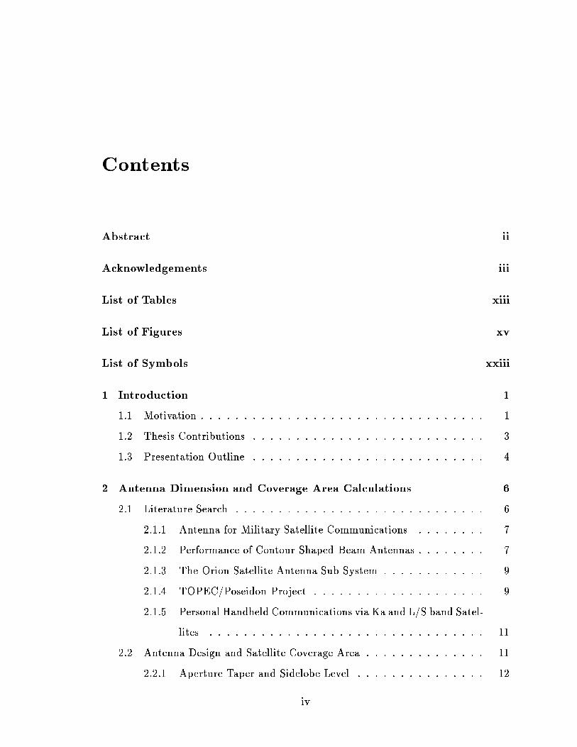
Contents

Abstract ii

Acknowledgements iii

List of Tables xiii

List of Figures xv

List of Symbols xxiii

1 Introduction 1

1.1 Motivation : : : : : : : : : : : : : : : : : : : : : : : : : : : : : : : : : 1

1.2 Thesis Contributions : : : : : : : : : : : : : : : : : : : : : : : : : : : 3

1.3 Presentation Outline : : : : : : : : : : : : : : : : : : : : : : : : : : : 4

2 Antenna Dimension and Coverage Area Calculations 6

2.1 Literature Search : : : : : : : : : : : : : : : : : : : : : : : : : : : : : 6

2.1.1 Antenna for Military Satellite Communications : : : : : : : : 7

2.1.2 Performance of Contour Shaped Beam Antennas : : : : : : : : 7

2.1.3 The Orion Satellite Antenna Sub-System : : : : : : : : : : : : 9

2.1.4 TOPEC/Poseidon Project : : : : : : : : : : : : : : : : : : : : 9

2.1.5 Personal Handheld Communications via Ka and L/S band Satel-

lites : : : : : : : : : : : : : : : : : : : : : : : : : : : : : : : : 11

2.2 Antenna Design and Satellite Coverage Area : : : : : : : : : : : : : : 11

2.2.1 Aperture Taper and Sidelobe Level : : : : : : : : : : : : : : : 12

iv

2.2.2 Beamwidth : : : : : : : : : : : : : : : : : : : : : : : : : : : : 12

2.2.3 Gain Loss : : : : : : : : : : : : : : : : : : : : : : : : : : : : : 14

2.2.4 Oset Height : : : : : : : : : : : : : : : : : : : : : : : : : : : 14

2.2.5 Maximum Scan Angle : : : : : : : : : : : : : : : : : : : : : : 14

2.3 Calculated Dimension for the Re ector Antenna : : : : : : : : : : : : 15

2.3.1 Re ector Diameter : : : : : : : : : : : : : : : : : : : : : : : : 15

2.3.2 Focal Length : : : : : : : : : : : : : : : : : : : : : : : : : : : 15

2.3.3 Gain : : : : : : : : : : : : : : : : : : : : : : : : : : : : : : : : 15

2.3.4 Re ector Angle : : : : : : : : : : : : : : : : : : : : : : : : : : 16

2.3.5 Feed Directivity Value (Q) : : : : : : : : : : : : : : : : : : : : 16

2.3.6 Element Size and Spacing : : : : : : : : : : : : : : : : : : : : 17

2.3.7 Antenna Design Summary : : : : : : : : : : : : : : : : : : : : 17

2.4 Feed Location Calculation : : : : : : : : : : : : : : : : : : : : : : : : 19

2.5 Beam Distortion due to Frequency Distribution : : : : : : : : : : : : 20

2.6 Degradation in Performance for O Focus Beams : : : : : : : : : : : 22

3 Link Budget Calculation for the Ka-Band Geostationary Satellite 27

3.1 Ka-Band Link Budget Contributions : : : : : : : : : : : : : : : : : : 27

3.1.1 Physical Link Parameter Summary : : : : : : : : : : : : : : : 29

3.1.2 Earth/Satellite EIRP : : : : : : : : : : : : : : : : : : : : : : : 30

3.1.3 Free Space Loss : : : : : : : : : : : : : : : : : : : : : : : : : : 31

3.1.4 Gaseous Losses : : : : : : : : : : : : : : : : : : : : : : : : : : 31

3.1.5 Rain Attenuation : : : : : : : : : : : : : : : : : : : : : : : : : 32

3.1.6 Temperature : : : : : : : : : : : : : : : : : : : : : : : : : : : : 32

3.1.7 Bandwidth Calculation : : : : : : : : : : : : : : : : : : : : : : 32

3.2 FDMA System : : : : : : : : : : : : : : : : : : : : : : : : : : : : : : 33

3.3 Link Budget Calculation : : : : : : : : : : : : : : : : : : : : : : : : : 33

3.3.1 Hardware Specications : : : : : : : : : : : : : : : : : : : : : 34

3.3.2 Frequency Parameters : : : : : : : : : : : : : : : : : : : : : : 34

3.3.3 Target Latitude and Longitude : : : : : : : : : : : : : : : : : 34

v

3.3.4 Height above Sea Level : : : : : : : : : : : : : : : : : : : : : : 35

3.3.5 Outage Percentage : : : : : : : : : : : : : : : : : : : : : : : : 35

3.3.6 Antenna Gain Reduction : : : : : : : : : : : : : : : : : : : : : 35

3.3.7 System Interference : : : : : : : : : : : : : : : : : : : : : : : : 35

3.3.8 Temperature Parameters : : : : : : : : : : : : : : : : : : : : : 36

3.3.9 Channel Guard Bands : : : : : : : : : : : : : : : : : : : : : : 36

3.3.10 Pulse Design : : : : : : : : : : : : : : : : : : : : : : : : : : : 37

3.3.11 Base Band Channel : : : : : : : : : : : : : : : : : : : : : : : : 37

3.3.12 Ionospheric Eects : : : : : : : : : : : : : : : : : : : : : : : : 37

3.3.13 E

b

=N

o

Requirements : : : : : : : : : : : : : : : : : : : : : : : 37

3.4 Comparison with L Band Voice System : : : : : : : : : : : : : : : : : 40

4 Cyclostationary Beamforming and On-Board Processing 42

4.1 Motivation for Digital Beamforming and On-Board Processing : : : : 42

4.1.1 Reference-Based Beamforming : : : : : : : : : : : : : : : : : : 43

4.1.2 Location-Based Beamforming : : : : : : : : : : : : : : : : : : 44

4.1.3 Property Restoral/Blind Beamforming : : : : : : : : : : : : : 44

4.2 Motivation for the Cyclostationary Property Restoral Technique : : : 45

4.3 Theoretical Background for Cyclostationary Analysis : : : : : : : : : 46

4.3.1 Fraction of Time Probability Measure : : : : : : : : : : : : : : 47

4.4 Second-Order Cyclostationariy : : : : : : : : : : : : : : : : : : : : : : 50

4.4.1 Cyclic Autocorrelation Function : : : : : : : : : : : : : : : : : 51

4.5 Cyclic Temporal Correlation Coecient : : : : : : : : : : : : : : : : : 53

4.6 Spectral Correlation Density Function : : : : : : : : : : : : : : : : : 53

4.7 Frequency-Shift Filtering (FRESH) : : : : : : : : : : : : : : : : : : : 54

4.8 The Cyclic Signal Model Environment : : : : : : : : : : : : : : : : : 55

4.9 Blind Cyclic Spatial Filtering Algorithms : : : : : : : : : : : : : : : : 57

4.9.1 Spectral Coherence Restoral Blind Beamforming Algorithms

(SCORE) : : : : : : : : : : : : : : : : : : : : : : : : : : : : : 57

4.9.2 The Cyclic Adaptive Beamforming Algorithm : : : : : : : : : 62

vi

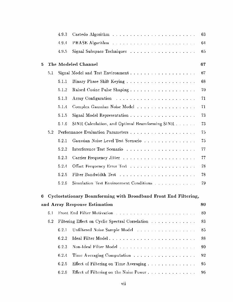
4.9.3 Castedo Algorithm : : : : : : : : : : : : : : : : : : : : : : : : 63

4.9.4 PHASE Algorithm : : : : : : : : : : : : : : : : : : : : : : : : 64

4.9.5 Signal Subspace Techniques : : : : : : : : : : : : : : : : : : : 65

5 The Modeled Channel 67

5.1 Signal Model and Test Environment : : : : : : : : : : : : : : : : : : : 67

5.1.1 Binary Phase Shift Keying : : : : : : : : : : : : : : : : : : : : 68

5.1.2 Raised Cosine Pulse Shaping : : : : : : : : : : : : : : : : : : : 70

5.1.3 Array Conguration : : : : : : : : : : : : : : : : : : : : : : : 71

5.1.4 Complex Gaussian Noise Model : : : : : : : : : : : : : : : : : 71

5.1.5 Signal Model Representation : : : : : : : : : : : : : : : : : : : 73

5.1.6 SINR Calculation, and Optimal Beamforming SINR : : : : : : 73

5.2 Performance Evaluation Parameters : : : : : : : : : : : : : : : : : : : 75

5.2.1 Gaussian Noise Level Test Scenario : : : : : : : : : : : : : : : 75

5.2.2 Interference Test Scenario : : : : : : : : : : : : : : : : : : : : 77

5.2.3 Carrier Frequency Jitter : : : : : : : : : : : : : : : : : : : : : 77

5.2.4 Oset Frequency Error Test : : : : : : : : : : : : : : : : : : : 78

5.2.5 Filter Bandwidth Test : : : : : : : : : : : : : : : : : : : : : : 78

5.2.6 Simulation Test Environment Conditions : : : : : : : : : : : : 79

6 Cyclostationary Beamforming with Broadband Front End Filtering,

and Array Response Estimation 80

6.1 Front End Filter Motivation : : : : : : : : : : : : : : : : : : : : : : : 80

6.2 Filtering Eect on Cyclic Spectral Correlation : : : : : : : : : : : : : 83

6.2.1 Unltered Noise Sample Model : : : : : : : : : : : : : : : : : 85

6.2.2 Ideal Filter Model : : : : : : : : : : : : : : : : : : : : : : : : : 88

6.2.3 Non-Ideal Filter Model : : : : : : : : : : : : : : : : : : : : : : 90

6.2.4 Time Averaging Computation : : : : : : : : : : : : : : : : : : 92

6.2.5 Eect of Filtering on Time Averaging : : : : : : : : : : : : : : 95

6.2.6 Eect of Filtering on the Noise Power : : : : : : : : : : : : : : 96

vii

6.2.7 Limit as the Filter Bandwidth Approaches Innity : : : : : : 96

6.2.8 Limit as the Filter Bandwidth Approaches Zero : : : : : : : : 97

6.2.9 Finite Time Fourier Transform : : : : : : : : : : : : : : : : : 98

6.2.10 Summary of Filtering's Eects on Beamforming : : : : : : : : 99

6.3 Cyclostationary Array Response Estimation : : : : : : : : : : : : : : 101

6.4 Front End Filtered SCORE Beamforming Techniques : : : : : : : : : 103

6.4.1 SCORE Algorithm (SCORE) : : : : : : : : : : : : : : : : : : 106

6.4.2 Filtered SCORE Algorithm (F-SCORE) : : : : : : : : : : : : 106

6.4.3 Phase Compensated SCORE Algorithm (PC-SCORE) : : : : 106

6.4.4 Array Estimated SCORE (A-SCORE) : : : : : : : : : : : : : 107

6.4.5 Filtered Array Estimated SCORE (FA-SCORE) : : : : : : : : 107

6.5 Transitional Filter Design : : : : : : : : : : : : : : : : : : : : : : : : 107

7 SCORE Algorithm Simulation Results 112

7.1 Introduction : : : : : : : : : : : : : : : : : : : : : : : : : : : : : : : : 112

7.2 Cyclostationary Array Estimation Performance of the Linear and Parabolic

Antenna Conguration : : : : : : : : : : : : : : : : : : : : : : : : : : 113

7.3 Eect of Array Initialization : : : : : : : : : : : : : : : : : : : : : : : 118

7.4 Performance Comparison between Cross SCORE and Least Squares

SCORE : : : : : : : : : : : : : : : : : : : : : : : : : : : : : : : : : : 119

7.4.1 Summary of Filtered Least Square and Cross SCORE algorithm

Comparison : : : : : : : : : : : : : : : : : : : : : : : : : : : : 127

7.5 Comparison of the Parabolic and Linear Arrays : : : : : : : : : : : : 127

7.6 Beam Pattern Performance : : : : : : : : : : : : : : : : : : : : : : : : 128

7.7 SCORE Algorithm Convergence Performance : : : : : : : : : : : : : 130

7.7.1 Eect of Filter Bandwidth on Convergence Performance : : : 130

7.8 Eect of Noise on Convergence Performance : : : : : : : : : : : : : : 137

7.8.1 Convergence Rate Deterioration due to Noise : : : : : : : : : 139

7.8.2 SCORE Convergence Limit due to High Noise : : : : : : : : : 139

7.8.3 Cross SCORE Noise Performance Summary : : : : : : : : : : 139

viii

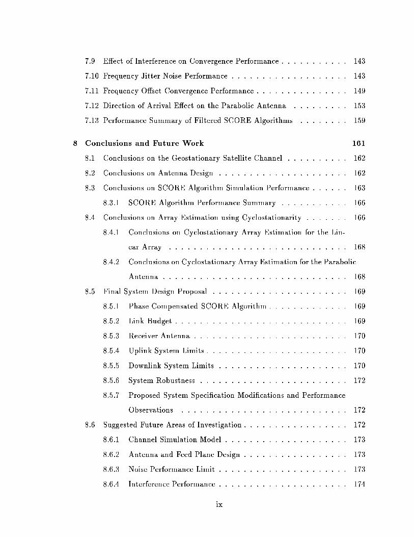
7.9 Eect of Interference on Convergence Performance : : : : : : : : : : : 143

7.10 Frequency Jitter Noise Performance : : : : : : : : : : : : : : : : : : : 143

7.11 Frequency Oset Convergence Performance : : : : : : : : : : : : : : : 149

7.12 Direction of Arrival Eect on the Parabolic Antenna : : : : : : : : : 153

7.13 Performance Summary of Filtered SCORE Algorithms : : : : : : : : 159

8 Conclusions and Future Work 161

8.1 Conclusions on the Geostationary Satellite Channel : : : : : : : : : : 162

8.2 Conclusions on Antenna Design : : : : : : : : : : : : : : : : : : : : : 162

8.3 Conclusions on SCORE Algorithm Simulation Performance : : : : : : 163

8.3.1 SCORE Algorithm Performance Summary : : : : : : : : : : : 166

8.4 Conclusions on Array Estimation using Cyclostationarity : : : : : : : 166

8.4.1 Conclusions on Cyclostationary Array Estimation for the Lin-

ear Array : : : : : : : : : : : : : : : : : : : : : : : : : : : : : 168

8.4.2 Conclusions on Cyclostationary Array Estimation for the Parabolic

Antenna : : : : : : : : : : : : : : : : : : : : : : : : : : : : : : 168

8.5 Final System Design Proposal : : : : : : : : : : : : : : : : : : : : : : 169

8.5.1 Phase-Compensated SCORE Algorithm : : : : : : : : : : : : : 169

8.5.2 Link Budget : : : : : : : : : : : : : : : : : : : : : : : : : : : : 169

8.5.3 Receiver Antenna : : : : : : : : : : : : : : : : : : : : : : : : : 170

8.5.4 Uplink System Limits : : : : : : : : : : : : : : : : : : : : : : : 170

8.5.5 Downlink System Limits : : : : : : : : : : : : : : : : : : : : : 170

8.5.6 System Robustness : : : : : : : : : : : : : : : : : : : : : : : : 172

8.5.7 Proposed System Specication Modications and Performance

Observations : : : : : : : : : : : : : : : : : : : : : : : : : : : 172

8.6 Suggested Future Areas of Investigation : : : : : : : : : : : : : : : : : 172

8.6.1 Channel Simulation Model : : : : : : : : : : : : : : : : : : : : 173

8.6.2 Antenna and Feed Plane Design : : : : : : : : : : : : : : : : : 173

8.6.3 Noise Performance Limit : : : : : : : : : : : : : : : : : : : : : 173

8.6.4 Interference Performance : : : : : : : : : : : : : : : : : : : : : 174

ix

8.6.5 Frequency Jitter Performance : : : : : : : : : : : : : : : : : : 174

8.6.6 Oset Frequency Error : : : : : : : : : : : : : : : : : : : : : : 174

8.6.7 Filter Optimization : : : : : : : : : : : : : : : : : : : : : : : : 174

8.6.8 Cyclostationary Array Estimation : : : : : : : : : : : : : : : : 175

8.6.9 Low Earth Orbit Satellite Applications : : : : : : : : : : : : : 175

8.6.10 Terrestrial Applications : : : : : : : : : : : : : : : : : : : : : : 176

8.6.11 Algorithm Optimization : : : : : : : : : : : : : : : : : : : : : 176

A Antenna Design and Simulation Methods 177

A.1 Calculation of the Oset Parabolic Re ector Dimensions : : : : : : : 177

A.2 Design Procedure : : : : : : : : : : : : : : : : : : : : : : : : : : : : : 179

A.3 Approximate Radiation Pattern : : : : : : : : : : : : : : : : : : : : : 181

A.4 Antenna Pattern Program : : : : : : : : : : : : : : : : : : : : : : : : 182

A.4.1 Parabolic Antenna Theory and Approximations : : : : : : : : 182

A.4.2 Parameter Specication : : : : : : : : : : : : : : : : : : : : : 183

A.5 Feed Design : : : : : : : : : : : : : : : : : : : : : : : : : : : : : : : : 183

A.5.1 Maximum Theoretical Eciency of Multiple Beam Antennas : 184

A.5.2 Beamwidth of Antenna Feed Elements : : : : : : : : : : : : : 184

A.5.3 Wide Band Techniques for Antenna Feeds : : : : : : : : : : : 186

A.6 Filter Implementation : : : : : : : : : : : : : : : : : : : : : : : : : : 188

A.7 Transitional Filter Design : : : : : : : : : : : : : : : : : : : : : : : : 190

A.8 Butterworth Pole Location : : : : : : : : : : : : : : : : : : : : : : : : 190

A.9 Bessel Pole Location : : : : : : : : : : : : : : : : : : : : : : : : : : : 191

B Satellite Footprint Calculations 193

C Beam Patterns for O Focus Feeds 198

D Communications Model Background 202

D.1 Statistical Channel Model of the Carrier at the Ka Frequency Band : 203

D.2 Ionospheric Eects : : : : : : : : : : : : : : : : : : : : : : : : : : : : 205

x

D.2.1 Refraction/Direction of Arrival Variation : : : : : : : : : : : : 205

D.2.2 Faraday Rotation : : : : : : : : : : : : : : : : : : : : : : : : : 205

D.2.3 Group Delay : : : : : : : : : : : : : : : : : : : : : : : : : : : : 206

D.2.4 Phase Advance : : : : : : : : : : : : : : : : : : : : : : : : : : 206

D.2.5 Doppler Frequency : : : : : : : : : : : : : : : : : : : : : : : : 207

D.2.6 Dispersion : : : : : : : : : : : : : : : : : : : : : : : : : : : : : 207

D.2.7 Ionospheric Scintillation : : : : : : : : : : : : : : : : : : : : : 208

D.2.8 Summary of Ionospheric Eects : : : : : : : : : : : : : : : : : 208

D.3 Clear Air Eects : : : : : : : : : : : : : : : : : : : : : : : : : : : : : 209

D.4 Tropospheric Scattering : : : : : : : : : : : : : : : : : : : : : : : : : 209

D.5 Antenna Gain Reduction : : : : : : : : : : : : : : : : : : : : : : : : : 209

D.6 Absorptive Eects : : : : : : : : : : : : : : : : : : : : : : : : : : : : : 210

D.6.1 Absorption due to Oxygen : : : : : : : : : : : : : : : : : : : : 210

D.6.2 Absorption due to Water : : : : : : : : : : : : : : : : : : : : : 211

D.6.3 Total Gaseous Attenuation due to Absorption : : : : : : : : : 212

D.7 Tropospheric Scintillation Eects : : : : : : : : : : : : : : : : : : : : 213

D.8 Attenuation Eects : : : : : : : : : : : : : : : : : : : : : : : : : : : : 213

D.8.1 Attenuation Prediction Models : : : : : : : : : : : : : : : : : 214

D.9 Downlink Degradation : : : : : : : : : : : : : : : : : : : : : : : : : : 219

D.10 Frequency Scaling : : : : : : : : : : : : : : : : : : : : : : : : : : : : : 221

D.11 Fading Statistics : : : : : : : : : : : : : : : : : : : : : : : : : : : : : 223

E Coordinate System Transformations 226

E.1 Earth Centered System : : : : : : : : : : : : : : : : : : : : : : : : : : 226

E.2 Satellite Centered System : : : : : : : : : : : : : : : : : : : : : : : : 228

E.3 Perspective Projection View of the Earth : : : : : : : : : : : : : : : : 228

E.4 Coordinate Transform : : : : : : : : : : : : : : : : : : : : : : : : : : 229

E.5 Local Coordinate System : : : : : : : : : : : : : : : : : : : : : : : : : 231

E.6 Satellite / Earth Geometry : : : : : : : : : : : : : : : : : : : : : : : : 233

xi

F Calculation of Satellite Feed Coordinates 236

Bibliography 241

Vita 246

xii

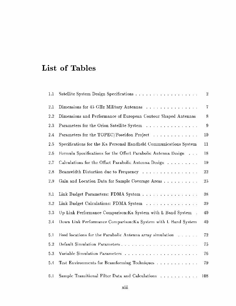
List of Tables

1.1 Satellite System Design Specications : : : : : : : : : : : : : : : : : : 2

2.1 Dimensions for 45 GHz Military Antennas : : : : : : : : : : : : : : : 7

2.2 Dimensions and Performance of European Contour Shaped Antennas 8

2.3 Parameters for the Orion Satellite System : : : : : : : : : : : : : : : 9

2.4 Parameters for the TOPEC/Poseidon Project : : : : : : : : : : : : : 10

2.5 Specications for the Ka Personal Handheld Communications System 11

2.6 Formula Specications for the Oset Parabolic Antenna Design : : : 18

2.7 Calculations for the Oset Parabolic Antenna Design : : : : : : : : : 19

2.8 Beamwidth Distortion due to Frequency : : : : : : : : : : : : : : : : 22

2.9 Gain and Location Data for Sample Coverage Areas : : : : : : : : : : 25

3.1 Link Budget Parameters: FDMA System : : : : : : : : : : : : : : : : 38

3.2 Link Budget Calculations: FDMA System : : : : : : : : : : : : : : : 39

3.3 Up Link Performance Comparison:Ka System with L Band System : 40

3.4 Down Link Performance Comparison:Ka System with L Band System 40

5.1 Feed locations for the Parabolic Antenna array simulation : : : : : : 72

5.2 Default Simulation Parameters : : : : : : : : : : : : : : : : : : : : : : 75

5.3 Variable Simulation Parameters : : : : : : : : : : : : : : : : : : : : : 76

5.4 Test Environments for Beamforming Techniques : : : : : : : : : : : : 79

6.1 Sample Transitional Filter Data and Calculations : : : : : : : : : : : 108

xiii

7.1 Direction of Arrival Information for the Parabolic Antenna: = 0:23

= 4:21

: : : : : : : : : : : : : : : : : : : : : : : : : : : : : : : : : 154

7.2 Direction of Arrival Information for the Parabolic Antenna: = 0:0

= 3:5

: : : : : : : : : : : : : : : : : : : : : : : : : : : : : : : : : : 154

8.1 SCORE SINR Convergence Summary: Parabolic Antenna : : : : : : 167

8.2 SINR Calculations of Proposed Satellite System : : : : : : : : : : : : 171

A.1 Antenna Parameters for the Oset Parabolic Antenna Program : : : 183

A.2 Feed Parameters for the Oset Parabolic Antenna Program : : : : : : 183

D.1 Statistical Data on Carrier Envelope Under Various Weather Patterns 204

D.2 Calculation Summary of Ionospheric Eects : : : : : : : : : : : : : : 208

D.3 Fading Duration Statistics: 15 dB Attenuation Threshold : : : : : : : 223

D.4 Fading Duration Statistics: 20 dB Attenuation Threshold : : : : : : : 224

xiv

List of Figures

2.1 a) Diagram of Antenna Parameters b) Diagram of Beampattern Pa-

rameters : : : : : : : : : : : : : : : : : : : : : : : : : : : : : : : : : : 13

2.2 Satellite Footprint Coverage of Canada, Dimensions in : : : : : : : 20

2.3 Feed Plane Element Location for Coverage of Canada : : : : : : : : : 21

2.4 Foot Print Distortion at 21 MHz : : : : : : : : : : : : : : : : : : : : 23

2.5 Foot Print Distortion at 19 MHz : : : : : : : : : : : : : : : : : : : : 23

2.6 Feed Location for O Focus Beam Pattern Foot prints : : : : : : : : 24

2.7 Beam Pattern of Feed 1 : : : : : : : : : : : : : : : : : : : : : : : : : 26

2.8 Beam Pattern of Feed 6 : : : : : : : : : : : : : : : : : : : : : : : : : 26

3.1 Diagram of Atmospheric Eects on the Channel : : : : : : : : : : : : 28

3.2 Allocation of Channels at the Ka Band : : : : : : : : : : : : : : : : : 36

5.1 Signal Processing before Beamforming : : : : : : : : : : : : : : : : : 68

5.2 a) Signal spectrum at the Ka Band. b) Analogue down conversion

of desired channel to the wide band anti-aliasing lter. c) Digitally

sampled spectrum of the desired channel. : : : : : : : : : : : : : : : : 69

6.1 a) Received waveform magnitude before ltering b) Received waveform

magnitude after ltering : : : : : : : : : : : : : : : : : : : : : : : : : 82

6.2 Processing Steps for Beamforming : : : : : : : : : : : : : : : : : : : : 86

6.3 a) Frequency Domain of the Noise Variance. b) Time Domain of Noise

Samples. : : : : : : : : : : : : : : : : : : : : : : : : : : : : : : : : : : 87

xv

6.4 a) Frequency domain magnitude of an ideal lter pulse. b) Frequency

domain phase of an ideal lter pulse. c) Time domain impulse response

of an ideal lter. : : : : : : : : : : : : : : : : : : : : : : : : : : : : : 89

6.5 a) Frequency domain magnitude of an non-ideal lter. b) Frequency

domain phase of an non-ideal lter. : : : : : : : : : : : : : : : : : : : 91

6.6 Components of a lter with non-ideal phase response : : : : : : : : : 92

6.7 Comparison of a ideal and non-ideal lter pulse in response showing

pulse widening. : : : : : : : : : : : : : : : : : : : : : : : : : : : : : : 93

6.8 a) SCORE beamforming implementation b) F-SCORE beamforming

implementation c) PC-SCORE beamforming implementation : : : : : 104

6.9 d)A-SCORE beamforming implementation e) FA-SCORE beamform-

ing implementation : : : : : : : : : : : : : : : : : : : : : : : : : : : : 105

6.10 Plot of S plane Poles and Zeros for Butterworth, Bessel, Transitional

Filters : : : : : : : : : : : : : : : : : : : : : : : : : : : : : : : : : : : 109

6.11 Plot of the Normalized Magnitude for Butterworth, Bessel, Transi-

tional Filters : : : : : : : : : : : : : : : : : : : : : : : : : : : : : : : : 109

6.12 Plot of the Normalized Phase for Butterworth, Bessel, Transitional

Filters : : : : : : : : : : : : : : : : : : : : : : : : : : : : : : : : : : : 110

7.1 Cyclic Array Estimation Linear Array SINR Test LNNB: Received

SINR=-12 dB. *-: Optimum SINR, x-:Single Element SINR. : : : : : 113

7.2 Cyclic Array Estimation: Element # 1 Phase Convergence Test LNNB:

Received SINR=-12 dB. *-: Optimum Angle : : : : : : : : : : : : : : 114

7.3 Cyclic Array Estimation: Element # 5 Phase Convergence Test LNNB:

Received SINR=-12 dB. *-: Optimum Angle : : : : : : : : : : : : : : 115

7.4 Cyclic Array Estimation Linear Array SINR Test HNNB: Received

SINR=-36 dB. *-: Optimum SINR, x-:Single Element SINR. : : : : : 115

7.5 Cyclic Array Estimation Parabolic Antenna: Element # 1 Phase Con-

vergence Test HNWB: Received SINR=-36 dB. *-: Optimum Angle : 116

xvi

7.6 Cyclic Array Estimation Parabolic Antenna: Element # 5 Convergence

Test HNWB Received SINR=-14 dB. *-: Optimum Angle : : : : : : : 117

7.7 Performance Comparison of Array Initialization for SCORE Algorithms.

*-: Optimum SNR, x-: Single Element SNR : : : : : : : : : : : : : : 120

7.8 LS-SCORE Linear Array SINR, Test LNNB. Received SNR=-12 dB.

*-: Optimum SINR, x-:Single Element SINR. : : : : : : : : : : : : : : 122

7.9 Cross-SCORE Linear Array SINR, Test LNNB. Received SNR=-12

dB. *-: Optimum SINR, x-:Single Element SINR. : : : : : : : : : : : 123

7.10 LS-SCORE Converged SINR Linear Array Noise Performance: Test

LNNB. *-: Optimum SINR, x-:Single Element SINR : : : : : : : : : : 123

7.11 Cross-SCORE Converged SINR Linear Array Noise Performance: Test

LNNB. *-: Optimum SINR, x-:Single Element SINR : : : : : : : : : : 124

7.12 LS-SCORE Parabolic Antenna SINR, Test LNNB. Received SNR=-36

dB. *-: Optimum SINR, x-:Single Element SINR. : : : : : : : : : : : 124

7.13 Cross-SCORE Parabolic Antenna SINR, Test LNNB. Received SNR=-

36 dB. *-: Optimum SINR, x-:Single Element SINR. : : : : : : : : : : 125

7.14 LS-SCORE Converged SINR Parabolic Antenna Noise Performance:

Test LNNB. *-: Optimum SINR, x-:Single Element SINR : : : : : : : 125

7.15 Cross-SCORE Converged SINR Parabolic Antenna Noise Performance:

Test LNNB. *-: Optimum SINR, x-:Single Element SINR : : : : : : : 126

7.16 CS-SCORE Parabolic Antenna Beam Pattern, Test LNNB. Received

SNR=-36 dB. *-: Optimum SINR. : : : : : : : : : : : : : : : : : : : 128

7.17 CS-SCORE Parabolic Antenna Beam Pattern, Test LNNB. Received

SNR=-36 dB. *-: Optimum SINR. : : : : : : : : : : : : : : : : : : : 129

7.18 Cross SCORE Parabolic Array SINR, Test LNNB: Received SNR=-36

dB. Filter BW= .05Hz. *-: Optimum SINR, x-: Single Element SINR 131

7.19 Cross SCORE Parabolic Array SINR, Test LNWB: Received SNR=-36

dB. Filter Bandwidth= .2 Hz *-: Optimum SINR, x-: Single Element

SINR : : : : : : : : : : : : : : : : : : : : : : : : : : : : : : : : : : : : 132

xvii

7.20 Cross SCORE Parabolic Array SINR, Test LNNB: Received SNR=-42


SINR : : : : : : : : : : : : : : : : : : : : : : : : : : : : : : : : : : : : 133

7.21 Cross SCORE Parabolic Array SINR, Test LNWB: Received SNR=-42


SINR : : : : : : : : : : : : : : : : : : : : : : : : : : : : : : : : : : : : 133

7.22 Cross SCORE Parabolic Antenna SINR, Test LNNB: Received SNR=-

40.4 dB. Filter Bandwidth= .4 Hz *-: Optimum SINR, x-: Single

Element SINR : : : : : : : : : : : : : : : : : : : : : : : : : : : : : : : 134

7.23 Cross SCORE Steady-State for SINR Parabolic Antenna, Test LNNB:

Received SNR=-40.4 dB. *-: Optimum SINR, x-: Single Element SINR 135

7.24 Cross SCORE Steady State for SINR Parabolic Antenna, Test HNNB:

Received SNR=-47 dB. *-: Optimum SINR, x-: Single Element SINR 136

7.25 Cross SCORE Steady-State for SINR Linear Array, Test LNNB: Re-

ceived SNR=-12 dB. *-: Optimum SINR, x-: Single Element SINR : 137

7.26 Cross SCORE Steady State for SINR Linear Array, Test HNNB: Re-

ceived SNR=-22 dB. *-: Optimum SINR, x-: Single Element SINR : 138

7.27 Cross-SCORE Parabolic Array SINR, Test LNWB. Received SNR=-36

dB. *-: Optimum SINR, x-: Single Element SINR : : : : : : : : : : : 140





7.30 Cross-SCORE Steady State SINR Parabolic Antenna Noise Perfor-

mance: Test LNWB. *-: Optimum SINR, x-: Single Element SINR : 142

7.31 Cross SCORE Parabolic Antenna Array SINR, Test LNNB. Interfer-

ence Frequency=.245 Hz with the desired oset frequency at .25 Hz.

*-: Optimum SINR, x-: Single Elements SINR. : : : : : : : : : : : : : 144

xviii

7.32 Cross SCORE Parabolic Antenna Array SINR, Test LNNB: Interfer-

ence Frequency=.2 Hz with the desired oset frequency at .25 Hz. *-:

Optimum SINR, x-: Single Elements SINR. : : : : : : : : : : : : : : 145

7.33 Cross SCORE Parabolic Antenna SINR, Test LNWB: Jitter Devia-

tion= 0.04 % of Carrier Oset Frequency (2 kHz). *-: Optimal SINR,

x-: Single Element SINR. : : : : : : : : : : : : : : : : : : : : : : : : : 146

7.34 Cross SCORE Parabolic Antenna SINR, Test HNWB: Jitter Devia-



7.35 Cross SCORE Parabolic Antenna SINR, Test LNNB: Jitter Devia-



7.36 Cross SCORE Parabolic Array SINR, Test LNWB: Frequency Error

= 0.04 % of Carrier Oset Frequency (2 kHz). *-: Optimum SINR, x-:

Single Element SINR. : : : : : : : : : : : : : : : : : : : : : : : : : : : 150

7.37 Cross SCORE Parabolic Array SINR, Test LNWB: Frequency Error



7.38 Cross SCORE Parabolic Array SINR, Test HNWB: Frequency Error



7.39 Cross SCORE Parabolic Antenna Performance: = 0

= 3:5

.

Received SINR=-36 dB. *-: Optimum SINR, x-: Single Element SINR. 155


= 3:5

.



= 3:5

.


xix

7.42 Cross SCORE Steady State SINR Parabolic Antenna Noise Perfor-

mance: = 0

= 3:5

. Received SINR=-50 dB. *-: Optimum SINR,


7.43 Cross SCORE Parabolic Antenna Beam Pattern: = 0

= 3:5

.

Received SINR=-50 dB. *-: Optimum SINR. : : : : : : : : : : : : : : 158

A.1 Oset Parabolic Antenna Schematic : : : : : : : : : : : : : : : : : : : 178

A.2 Simple Diagram of a Patch and Planar F Antenna : : : : : : : : : : : 186

A.3 Broad and Narrow band Filter Schematic for Message and Carrier Re-

covery : : : : : : : : : : : : : : : : : : : : : : : : : : : : : : : : : : : 189

B.1 Earth-Satellite Geometry for the Calculation of Beam Footprints : : : 194

C.1 Beam Pattern of Feed 1 : : : : : : : : : : : : : : : : : : : : : : : : : 198






D.1 Eect of Elevation Angle on Oxygen and Water attenuation at = 20

GHz : : : : : : : : : : : : : : : : : : : : : : : : : : : : : : : : : : : : 211

D.2 Eect of Frequency on Oxygen and Water attenuation : : : : : : : : 212

D.3 Schematic of Absorption Mechanisms : : : : : : : : : : : : : : : : : : 214

D.4 Eect of Elevation on Rain Attenuation : : : : : : : : : : : : : : : : : 215

D.5 Eect of Frequency on Rain Attenuation : : : : : : : : : : : : : : : : 216

D.6 Eect of Height Above Sea Level on Rain Attenuation : : : : : : : : 217

D.7 Eect of Percent Outage Level on Rain Attenuation : : : : : : : : : : 218

D.8 Down Link Degradation Mechanism : : : : : : : : : : : : : : : : : : : 219

D.9 Antenna Noise Schematic : : : : : : : : : : : : : : : : : : : : : : : : : 220

E.1 Earth Coordinate system Geometry : : : : : : : : : : : : : : : : : : : 227

xx

E.2 Satellite Coordinate system Geometry : : : : : : : : : : : : : : : : : 228

E.3 Satellite Coordinate system Geometry : : : : : : : : : : : : : : : : : 229

E.4 Local Coordinate system Geometry : : : : : : : : : : : : : : : : : : : 232

E.5 Satellite-Earth Geometric relationship : : : : : : : : : : : : : : : : : : 234

F.1 Earth-Satellite Target Geometry : : : : : : : : : : : : : : : : : : : : : 236

F.2 Antenna Feedplane Geometry, Y-Plane : : : : : : : : : : : : : : : : : 237

F.3 Antenna Feed Plane Geometry, XZ-Plane : : : : : : : : : : : : : : : : 238

F.4 Geometry of Polar Coordinate Transform : : : : : : : : : : : : : : : : 240

xxi

List of Symbols

C=N ) Carrier to noise power ratio (dBm)

P

t

) Power transmitted (mW)

G

Sat

) Satellite Antenna Gain (dB)

G

Ea

) Earth Antenna Gain (dB)

L ) Total Loss (dB)

N

t

) Thermal Noise (dB)

A

A

) Antenna apperature (m

2

)

s

) Spillover eciency

o

) Manufacturing eciency

i

) Illumination eciency

) Wavelength (m)

SCORE ) SCORE simulation algorithm

F-SCORE ) Filtered SCORE simulation algorithm

FA-SCORE ) Filtered Array Estimated SCORE simulation algorithm

A-SCORE ) Array Estimated SCORE simulation algorithm

PC-SCORE ) Phase Compensated SCORE simulation algorithm

Array ) Cyclic Array Estimation Algorithm

F-Array ) Filtered Cyclic Array Estimation Algorithm

PC-Array ) Phase Compensated Cyclic Array Estimation Algorithm

LNNB ) Low Noise Narrow Band

LNWB ) Low Noise Wide Band

LNNB ) High Noise Narrow Band

HNWB ) High Noise Wide Band

xxiii

F ) Parent parabola focal length ()

h ) Height to center of re ector A ()

l

ant

) Re ector focal length ()

SL ) Sidelobe Level (dB)

1

) angle of x-z plane with re ector base (degrees)

2

) angle of x-z plane with re ector tip (degrees)

3

) angle of x-y plane with re ector center (degrees)

h

1

) oset height with respect to x-y plane ()

D ) Diameter of parent parabola (lambda)

D

1

) Diameter of re ector parabola ()

0

) the angle of the ray originating at the focus with

respect to the x-z componenet of the antenna boresight ()

1

) 3 dB angle (degrees)

) Wavelength

4 ) aperature taper (dB)

ET ) edge taper (dB)

3

) maximum scan angle (degrees)

BDF ) beam deviation factor

N ) Number of feeds.

A

ant

) center of the re ector

d

ant

) element spacing ()

Q ) Quality factor

f

hp

) Half power frequency

f

o

) Center frequency (Hz)

R

f

) Resistance of the feed

f

o


P

trans

) Complex Poles of the transitional lter

P

Btt

) Complex Poles of the Butterworth lter

P

Bss

) Complex Poles of the Bessel lter

W

Btt

) Weighting factor of the Butterworth lter

xxiv

W

Bss

) Weighting factor of the Bessel lter

Btt

) Butterworth scale factor for transfer function

k

Btt

) Transfer function of Butterworth lter

A

Btt

) Attenuation function of Butterworth lter

N

Btt

) Number of poles for Butterworth lter

N

Bssji

) Bessel lter polynomial, odd powers of frequency

M

Bssji

) Bessel lter polynomial, even powers of frequency

q

i

) coecients for the Bessel lter transfer function

Bss

) delay of Bessel lter

k ) Boltzman's constant (1:38 10

23

J=K)

T

e

) Noise temperature of Earth station (degrees K)

B ) Base band of signal (Hz)

T

s

) Sky noise temperature (degrees K)

P

s

) Satellite power (dB)

P

e

) Earth station power (dB)

G

s

) Satellite antenna gain (dB)

G

e

) Earth station antenna gain (dB)

L ) Link losses (dB)

L

w

) Weather losses (dB)

L

g

) Gaseous losses (dB)

L

f

) Free space losses (dB)

EIRP ) Equivilant Isotropic Radiated Power (dB)

f ) frequency (Hz)

N ) number of electrons =m

3

B

av

) average strength of earth's magnetic eld (Wb=m

3

)

dl ) incremental distance through plasma. (m)

TEC ) Total Electron Content (electrons=m

2

)

fd

) Faraday rotation (rad)

4t

i

) group delay (sec)

t

gd

) group delay across message bandwidth (sec)

xxv

pa

dt

) rate of change of phase advance (rad/sec)

4

pa

) phase advance (rad)

f

D

) Doppler frequency (Hertz)

pd

) phase dispersion (rad)

w

) water attenuation coecient (dB/km)

w

) water vapour (g/m

3

)

o

) oxygen attenuation coecient (dB/km)

h

o

) eective oxygen height (km)

h

w

) eective water vapour height (km)

h

wo

) eective water vapour scale coecient

h

s

) height above sea level (km)

h

R

) height of rain (km)

L

s

) slant path (km)

L

g

) horizontal slant path length (km)

r

x

) rain intensity reduciton factor

k

r

) rain attenuation coecient

r

) rain attenuation power term

el

) earth station elevation

r

) specic rain attenuation (dB/km)

A

g

) eective water vapour scale coecient

A

xjR

) attenuation level for a specic outage percent

R

0:01

) Point rainfall rate for the location for 0.01 percent

of an average year (mm/hr)

T

sys

) System noise temperature. (

K)

T

A

) Noise temperature incident on antenna. (

K)

T

r

) Receiver noise temperature (

K)

T

c

) Cosmic noise temperature (

K)

T

m

) Temperature of the medium (

K)

f

) Feed transmissivity factor

A

sky

) Total atmospheric attenuation (dB)

xxvi

A

g

) Gaseous attenuation (dB)

RAS ) rain attenuation statistical ratio

ACA ) attenuation due to clear air (dB)

f

u

) upper frequency (Hz)

f

l

) lower frequency (Hz)

G ) gravitational constant (6.67 10

11

)

M ) earth mass (kg) (5.976 1024)

P ) earth period (sec) (86, 164)

R ) earth mean radius (km) (6371)

~

f ) intersection point of ray from satellite with earth.

~

t ) ray from satellite to intersection point f.

~s ) ray from the earth center to the satellite.

A

T

) the target satellite point on the earth.

A

0

T

) projection of the satellite point on the earth x-y plane

d

1

) distance from satellite position S to target location A.

d

2

) distance from satellite position S to target projection A

0

T

.

es

) earth satellite longitudinal position

eA

) earth aim point longitudinal position

eA

) earth aim point latitudinal position

bw

) spherical coordinate of ray

~

t in z

a

y

a

plane restricted by beam width

bw

) spherical coordinate of ray

~

t in z

a

x

a

plane restricted by beam width

ef

) intersection point of satellite ray's longitudinal position

ef

) intersection point of satellite ray's latitudinal position

x

e

; y

e

; z

e

) earth cartesian coordinates

x

L

; y

L

; z

L

) local cartesian coordinates

x

s

; y

s

; z

s

) satellite cartesian coordinates

e

;

e

) earth spherical coordinates

s

;

s

) satellite spherical coordinates

~r;~s;

~

t ) orientation vectors for cartesian coordinate transform

~

i;

~

j;

~

k ) basis vectors for earth cartesian system

xxvii

~

l; ~m;~n ) basis vectors for earth local system

A ) cartesian transformation matrix

a

i

) element of cartesian transformation matrix

M

i

) scalar magnitudes of transformation matrix

es

) azimuth angle of earth to satellite

es

) elevation angle of earth to satellite

BDF ) beam deviation factor.

r

) angle re ected o of the re ector

a

) angle of the feed plane normal with the zy satellite plane

r

) angle re ected o of the re ector in the yz plane

a

) angle of rotation of the antenna coordinates with respect to the

satellite system in the xz plane

N

f

) normal vector of feed plane

~x

da

; ~y

da

; ~z

da

) direction vector with respect to cartesian coordinates

~

V

d

) direction vector with respect to cartesian coordinates

~x

ra

; ~y

ra

; ~z

ra

) cartesian coordinates of ray re ected o of re ector

~v

r

) cartesian coordinates of ray re ected o of re ector

a

) angle of re ection of incident ray for an on focus beam

in the xz plane of the antenna

t

feed

) scaling parameter to nd the

intersection point of the ray with the feed plane

feed

) angular component of the polar intersection point on the feed plane

feed

) radial component of the polar intersection point on the feed plane

u ) dummy frequency

) Fourier frequency

T

FA

) Fourier Time average period

v

l

) ltered signal

x(t) ) unltered signal

s(t) ) deterministic desired signal

f

c

) desired signal frequency

xxviii

jA

sig

j ) deterministic desired signal magnitude

jA

sinc

j ) sinc() attenuation factor

jA

filt

j ) lter attenuation factor

) deterministic phase of desired signal

i(t) ) deterministic interference signal

% ) deterministic phase of interference signal

jIj ) deterministic interference magnitude

n(t) ) random noise vector

jN

l

(t; f)j ) white Gausian noise N(0;

n

) from element l.

) uniformly distributed noise phase [; pi]

h(t) ) time domain response of lter

jH(f)j ) frequency response magnigude of lter

(f) ) frequency phase response of lter

B

filt

) lter bandwidth

B

FA

) Fourier time average lter bandwidth

T

FA

) coecient for the sinc function of the nite time Fourier transform

T

FA

) maximum magnitude of the nite time Fourier transform with T

FA

= 0

filt

) phase error constant of the lter

N

B

FA

) number of discrete frequencies for in the interval B

FA

.

) lter phase error due to

filt

N

4t

;K

) Correlation coecient sum.

) time averaged mean

c

(i k) ) correlation between elements.

xxix

Chapter 1

Introduction

1.1 Motivation

There is an increasing demand for broadband services which will provide reliable

transmission of information. Multi-media applications including data and video re-

quire large bandwidths and low error rates for satisfactory performance. This demand

will exceed the present services in existence today, and there will be increasing prob-

lems nding the required frequency spectrum to provide the bandwidth for broadband

services. Below is a summary of some of the obstacles that the design and deployment

of a broadband system will have to overcome.

An accurate model of the channel environment must be developed which will

predict how the transmitted signals would be degraded.

High frequency spectral bands will have to be used to provide the necessary

bandwidth for the system.

In order to keep the transmitter and receiver small, power resources must be

conserved.

The system must be robust to component failure, and errors introduced by the

channel.

The service provided to the coverage area must be uniform.

1

A dynamic access scheme needs to be considered which will adapt to changes

in the user location, and in the channel environment.

To meet these system requirements a geostationary satellite system is proposed.

The target specications of this system are presented in Table 1.1.

Parameter Specication

Downlink Frequency 20 GHz

Uplink Frequency 30 GHz

Coverage Area Canada

BER 10

5

Number of Users 100

Bit Rate 2 Mbps

Uplink Transmitter Power 1 W

Downlink Transmitter Power 1 W

User Location Portable

Table 1.1: Satellite System Design Specications

In order to meet these specications, the following techniques will be employed:

The Ka frequency band will be used. The spectrum at this frequency is presently

unallocated, and has the necessary size to support a broadband service. Band-

width will not be a limiting parameter.

A multi-beam geostationary satellite will provide the necessary coverage. This

satellite system will use a parabolic antenna to increase the SNR of the signal.

Beamforming will be investigated using the Spectral Self Coherence Property

Restoral technique (SCORE). A new technique using front end ltering and ar-

ray estimation will be applied to the SCORE algorithm to improve performance

and robustness.

2

The use of the Ka frequency band has the advantage of providing the necessary

spectrum. The drawback is that higher frequencies suer more from attenuation

due to free space losses and atmospheric attenuation. The present literature is only

beginning to focus on characterizing the Ka frequency band, and there is very little

long term data available for modeling.

The multi-beam parabolic antenna conguration seeks to compensate the high

attenuation resulting from using the Ka frequency band. The parabolic antenna

oers a large gain. Parabolic antenna construction can be light-weight which will

keep the payload of the system small.

The use of beamforming is aimed at maximizing the satellites resources. A beam-

forming algorithm will allow for agile formation of spot beams which can adaptively

focus on a user's location, and respond to a time varying channel environment. The

ability to dynamically focus the satellite beam could be used to reduce power and

hardware requirements, or to increase the system performance.

The SCORE algorithm is seen as ideal for the satellite beamforming application.

This algorithm uses the cyclostationary properties of the desired signal to beamform.

As a result, no synchronization, training sequences, or array calibration are needed.

1.2 Thesis Contributions

This thesis has investigated several new areas with respect to satellite beamforming.

A channel model for the Ka frequency band is constructed. This channel shows

that the FDM access system proposed in this thesis is noise limited. Access

schemes studied in present literature are usually interference limited.

The Least Squares and Cross SCORE algorithm are applied to a parabolic an-

tenna array under high noise conditions (SNR < 30 dB). Previous work using

SCORE had always employed linear arrays in interference limited environments,

under low noise conditions (SNR > 0 dB).

3

Front-end ltering is employed to isolate the desired oset carrier frequency

needed for beamforming. Front-end ltering was shown to improve the perfor-

mance of the SCORE algorithms in high noise environments.

An estimation technique of the array response is presented. This algorithm

maximizes the real component of the cyclic autocorrelation value between an-

tenna elements by introducing a delay. The delay corresponds to a phase shift

which can be calculated. The cyclic array estimation technique was shown to

work for SNR levels of about -12 dB on linear arrays.

Initialization of the antenna elements to an estimate of the array response was

shown to have no signicant eect on the convergence rate of the SCORE algo-

rithms.

1.3 Presentation Outline

There are two distinct areas of research in this thesis. The rst aspect focuses on

the modeling of the satellite link at the Ka frequency band. The second section deals

with the beamforming algorithms and the test scenarios.

Chapter 2 presents the design and calculation of the parabolic antenna which will

be used in the satellite link. Based on the design of the antenna, a uniform coverage

area of Canada is calculated. This coverage area provides information on the amount

of physical hardware needed.

The system link budget is calculated in Chapter 3. The signicant channel atten-

uation factors for the link are presented for the Ka frequency band.

Chapter 4 presents the theory behind the cyclostationary algorithms. Several

dierent cyclostationary beamforming techniques are brie y presented.

The signal model for the simulations is described in Chapter 5. This includes

the noise modeling, modulation format, and simulation parameters. The selected

parameters for evaluating the robustness of the SCORE algorithms are also presented.

4

A technique of combining front-end ltering with cyclostationary beamforming is

presented in Chapter 6. A method of array response estimation is outlined, and the

simulation conditions are dened. The nal section of this chapter deals with the

design of the transitional lter to be used in the simulations.

Chapter 7 presents the results of the beamforming algorithm performance under

the test conditions chosen. Conclusions based on these test results are presented in

Chapter 8.

Appendix A, B and C present a calculation of the antenna design, coverage area

calculations and performance values. A detailed account of the channel model design

is presented in Appendix D.

Reference coordinate system derivations and translations are presented in Appen-

dices E and F.

5

Chapter 2

Antenna Dimension and Coverage Area

Calculations

This chapter outlines the calculation of the antenna dimensions and the required hard-

ware to provide uniform coverage of Canada. The antenna will be designed to work

at the Ka band frequency and will provide broadband services to the coverage area.

These models are used to determine worst case conditions within the coverage area.

The antenna gain and array patterns based on the calculated antenna dimensions are

used in all beamforming simulations and in link budget calculations.

A detailed presentation of the design procedures, and approximations used in

generating the antenna dimensions and beampatterns is presented in Appendix A.

Models and reference systems used in calculating the satellite foot print coverage,

and feed location calculations are presented in Appendices B and E.

2.1 Literature Search

In order to get an idea of the parameters of the system which are physically realizable

using current technology, an extensive search was done on satellite projects which are

already designed or implemented. The result of this search provided guidelines in

selecting the physical antenna parameters.

6

2.1.1 Antenna for Military Satellite Communications

In the paper by Rao [33], a satellite antenna was designed, and a prototype con-

structed which used a feed array of 121 Potter horn feed elements to cover a circular

region of 8

radius at 45 GHz modulating frequency. The design used 1

spot beams

which were grouped into a hexagonal septet to form a "virtual" feed and a resulting

beam footprint. This allowed beamforming to take place by weighting these feeds.

The system achieved a beam crossover level of 3 dB, and a sidelobe level of 25

dB below the peak gain. The interference nulling capability achieved nulls of 32 dB

below the main lobe. The satellite dimensions are shown bellow in units of wavelength.

Dimension Measurement ()

Diameter 83.4

Focal Length 140

Oset Height 22.36

Feed Horn Size 2.1

Gain (dB) 43.1

Table 2.1: Dimensions for 45 GHz Military Antennas

2.1.2 Performance of Contour Shaped Beam Antennas

There are several European satellite systems which employ shaped re ectors which

result in contour beam patterns. The design has the advantage of being practically

simple to implement, and the reduced number of feeds greatly reduces the mass of the

system. This design did not give the exibility of multiple access and beamforming

which is the thrust of this thesis. Below are a list of existing, or designed contour

beam systems which can be used to compare the performance of the multi-beam

system proposed in this thesis [30].

7

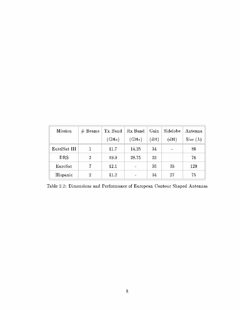
Mission # Beams Tx Band Rx Band Gain Sidelobe Antenna

(GHz) (GHz) (dB) (dB) Size ()

EutelSat III 1 11.7 14.25 34 - 80

DRS 2 19.0 28.75 23 - 76

EuroSat 7 12.1 - 35 35 120

Hispanic 2 11.2 - 34 27 75

Table 2.2: Dimensions and Performance of European Contour Shaped Antennas

8

2.1.3 The Orion Satellite Antenna Sub-System

This satellite project operates at the Ku band and uses two beam forming networks

to service America and Europe. The feed array is used to re-congure the antenna

beam patterns. The design accounts for antenna feed coupling. The system links

with ground terminals which use a 1.2 m rooftop antenna system. The satellite link

uses 100 W of power for each feed. Below is a summary of the design specications

[43].

Parameter American Beam European Beam

Diameter () 91.6 57.7

Focal Length () 75.7 47.7

Oset () 8 47.7

Tx Band (GHz) 11.95 12.1

Rx Band (GHz) 14.25 14.25

Gain (dB) 41 41

Feed Horns 12 8

Table 2.3: Parameters for the Orion Satellite System

The power requirements and the size of the receiving antenna make this style of

design poor for the portable low power system proposed in this thesis.

2.1.4 TOPEC/Poseidon Project

This project's objective is to accurately measure and collect data from the earth's

oceans. Below is a summary of the signicant parameters of the satellite. [47]

The largest power drain of this system comes from the traveling wave tube am-

plier (70 W). The signal processor is the next largest power user (37.4 W).

Power requirement data from this project indicate that a signicant amount of

the satellite's resources will have to be allocated to running the digital beamforming

hardware.

9

Parameter Measurement

Frequency (GHz) 13.6

Antenna Diameter () 68

Peak Power (W) 232

Gain (dB) 43.9

Table 2.4: Parameters for the TOPEC/Poseidon Project

10

2.1.5 Personal Handheld Communications via Ka and L/S

band Satellites

Design guidelines for portable voice systems operating in the Ka and L/S frequency

bands are presented in [13]. The following information is given for the Ka band

system.

Frequency (GHz) 20

3 dB Beamwidth 0.3

Antenna Diameter () 333

Antenna Gain (dB) 51.8

Transmitter Power (W) 7.8

Total number of cells 260

Total Power (W) 9192.91

Table 2.5: Specications for the Ka Personal Handheld Communications System

This system is designed to provided almost complete coverage of the United States

during clear sky conditions. During rain conditions a L band sub system (which suers

less from rain fades) takes over. The draw back of this system is the high number of

feeds required, and the large power demands of the system.

2.2 Antenna Design and Satellite Coverage Area

One of the goals of this thesis is to provide a system which would service all of

Canada. Simulations for coverage areas were made using designed programs, based

on geometric relations and approximations. These calculations are only rst order

[38], and do not incorporate detailed physical eects in antenna construction. Second-

order eects are not considered crucial to the system due to the fact that the cyclic

beamforming algorithms do not rely on the physical geometry of the system, and

provide adaptive beamforming weights to changing environmental conditions.

11

Calculations for the geometry of the oset parabolic antenna, a pattern of satellite

footprints to provide coverage of Canada, and the corresponding feed locations for

these footprints are presented in the following sections.

Preliminary calculations for the oset parabolic antenna are made using the de-

sign formulas presented in A.1, and the beampattern is veried using the program

developed by [11] (section A.4). The basic antenna design will cover Canada using a

hexagonal grid of antenna feeds. While this may not be the optimum conguration

for beamforming, it will oer a system that can be used for comparison with conven-

tional single beam per user systems, and will be able to show the relative gain due to

beamforming alone in these systems. The following subsections brie y dene some of

the design parameters and their eect on the antenna design. Figure 2.1 shows some

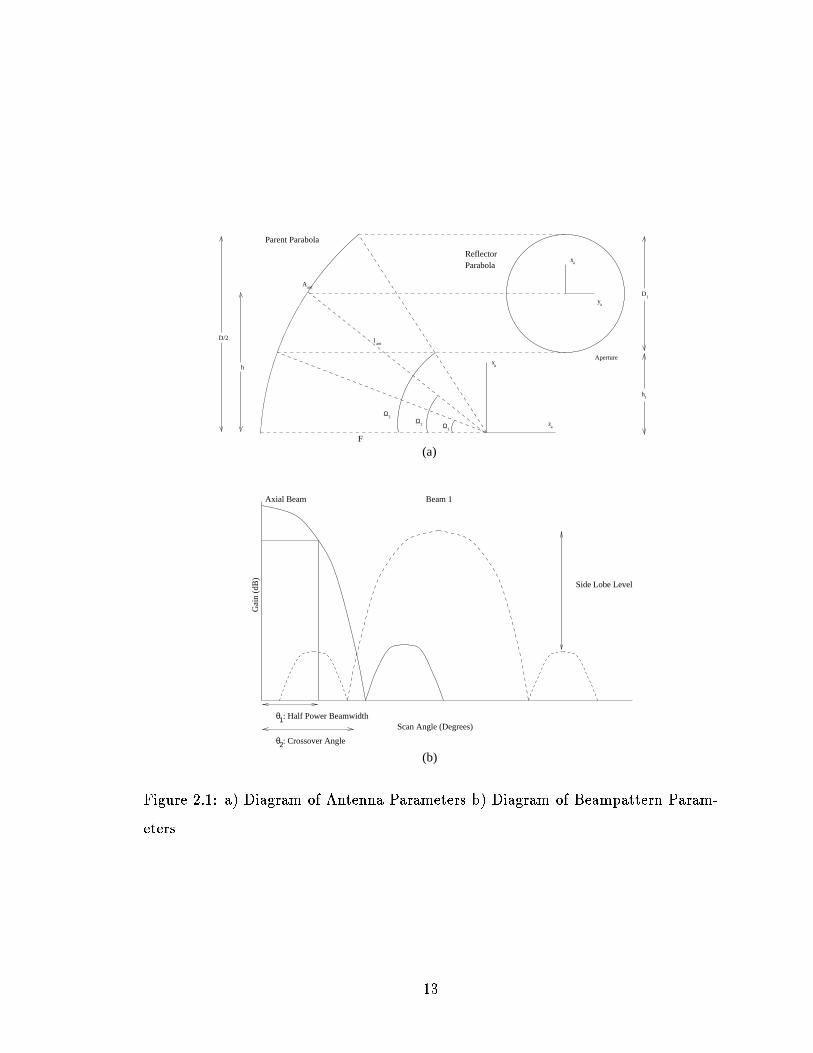
of the signicant antenna design dimensions and beampattern terms.

2.2.1 Aperture Taper and Sidelobe Level

The antenna's aperture taper measures the relative power level of the electric eld at

the center of the re ector with the power at the edge of the re ector. This in turn

determines the sidelobe level of an antenna. The sidelobe level is the magnitude of

the second maximum point after the mainlobe maximum. Low sidelobe levels are

desired to minimize the chance of amplifying signals which are not in the target area.

The sidelobe level directly in uences the aperture taper, which in turn controls

the size of the re ector. Levels ranging from 20 dB to 30 dB below the peak lobe gain

are used in existing systems. A specication of 27 dB was chosen for this project.

The 27 dB level gives the optimum edge taper performance for aperture eciency

as presented in [26]

2.2.2 Beamwidth

The beamwidth of the antenna greatly aects the antenna gain, and the size of the

re ector. The smallest practical beam that can be focussed accurately from a geo-

stationary satellite is 0:2

. The beamwidth is a parameter that is dependent on the

12

xa

Ω1

Ω2

Ω3

za

h1

D1

xa

ya

A

D/2

h

l

Aperture

ant

ant

θ1: Half Power Beamwidth

θ2: Crossover Angle

Axial Beam

Gai

n (d

B)

Scan Angle (Degrees)

Side Lobe Level

Beam 1

F

Parent Parabola

ReflectorParabola

(a)

(b)

Figure 2.1: a) Diagram of Antenna Parameters b) Diagram of Beampattern Param-

eters

13

frequency of the transmitted signal. For this reason all calculations are done in terms

of wavelengths, and then scaled to standard SI units depending on the frequency of

the application.

Since the largest possible gain is desired for this application, the 0:2

limit was

chosen as the design parameter.

2.2.3 Gain Loss

The gain loss parameter refers to the reduction in the main lobe gain as the antenna

feed is moved o of the focus of the x-z plane of the feed coordinate system (Appendix

F). The chosen gain loss greatly aects the focal length of the antenna and indirectly

aects the necessary size of the feed. A small gain loss results in a long focal length

and a larger, more directive feed.

The gain loss selected for this application is 0.1 dB. This level was found to give

a low loss while resulting in physical dimensions comparable to dimensions found in

the literature.

2.2.4 Oset Height

The oset height is dened as the number of wavelengths that the bottom edge of

the re ector is positioned above the y-z plane. This height is usually determined by

the size and orientation of the feed plane.

An oset height of 2 was found to provide enough clearance for the feed plane.

2.2.5 Maximum Scan Angle

The maximum scan angle is determined by the required coverage area of the system.

It is the largest angle in the x-z plane within the coverage area. The maximum scan

angle aects the focal length of the satellite.

The maximum scan angle for Canada was calculated. The antenna was directed

toward a target location of 94:7

Longitude and 51:4

Latitude. These dimensions

14

required a scan angle of 0:77

to provide coverage of Canada.

2.3 Calculated Dimension for the Re ector An-

tenna

Once the design parameters were selected, the antenna dimension calculations were

made. It was found that for these parameters, an antenna with dimensions compara-

ble to those found in literature was possible. Below is a comment on the signicance

of some of the calculated values.

2.3.1 Re ector Diameter

Present satellite systems have re ector parabolas approximately 3 m in diameter.

It was found that using the above design parameters that the downlink antenna

(20GHz operating frequency) would have the dimension of 2.5 m and the uplink (30

GHz operating frequency) would have the dimension of 1.67 m.

2.3.2 Focal Length

The focal lengths over 2.0 m are dicult to deploy. The design formulas indicated

that the focal length for the Uplink and Downlink antennas were 1.809 m and 1.206

m respectively. The shorter focal length also required a less directive, and smaller

feed.

2.3.3 Gain

The antenna gain was calculated using the antenna program developed in [11]. The

maximum achieved gain calculated was for the on focus feed, (feed position (0,0)),

was found to be 53.4 dB. The lowest gain for the coverage area was found to be 48.1

dB at a focal plane location of x = 1:165 and y = 8:869.

15

The pointing error associated with the 0:2

beamwidth is not expected to be

signicant for the beam forming application due to the fact that the calculated beam

will adjust to optimize the desired signal based on the direction of arrival.

The above calculated gain is comparable to the re ector antennas of existing

systems.

It was noticed during beamforming simulations that only two or three feed ele-

ments made signicant contributions to the combined signal depending on the location

of the target on the earth. Simulations were run using larger beamwidths with lower

gains to determine if such a system would have a better performance. The motivation

was that the larger beamwidths would allow more elements to contribute to the sum

after beamforming. The conclusion to this design was that the loss of gain could

not be compensated by the broader beamwidths of the adjacent elements. Further

investigation is needed in the area of optimizing the location of the antenna feeds for

the purpose of coverage and beamforming.

2.3.4 Re ector Angle

This is the angle that the center of the re ector makes with the focus and the z-y

plane of the satellite coordinate system. The feed plane is oriented perpendicular to

this angle.

The re ector angle was calculated to be 39

. This exceeds the recommended

design for the formulas which is 0

<

ref

< 30

. In order to decrease this angle it

would have been required to increase the focal length beyond practical dimensions.

The plotted beam patterns displayed no degradation in performance with respect

to the sidelobe levels or the gain due to the re ector angle.

2.3.5 Feed Directivity Value (Q)

The feed Q value controls the directivity of the antenna feed, and is responsible for

the edge taper. A more directive feed is required for long focal lengths or for low gain

16

losses. The required Q value for this conguration was found to be 6.62. Details of

this calculation are presented in Section A.3.

2.3.6 Element Size and Spacing

The paper [33] oered a method for calculating the element size for a specic Q value

based on the Potter Horn feed conguration.

The element size for the above designed antenna was calculated to be 0.903 .

This size was found to be small enough to t on the feed plane and provide coverage

of Canada. Dierent feed plane technologies, such as planar feeds, may also be able

to produce smaller feeds while still providing the necessary performance criteria.

A design was constructed which grouped feeds closer together than one wave-

length. The combined feed patterns for this system were found to be worse than

those for the larger element spacing design. This behavior was explained in the paper

by Lam et al. [24]

2.3.7 Antenna Design Summary

An oset parabolic antenna was designed which gives a minimum gain of 48.1 dB for

the furthest o focus antenna feed while giving a side lobe level of 27 dB below the

peak lobe. This gain was achieved for beamwidth of 0:2

.

Re ector size and focal length for both Uplink and Downlink designs were within

the dimensions of existing satellite systems. The feed size which resulted from the

calculations was small enough to t on the feed plane while providing enough coverage

to service any location in Canada.

This design will be used for all systems to be studied in this thesis.

17

Parameter Specication

Side Lobe (SL) (dB) 27

3dB

(deg) 0.2

Gain Loss (dB) 0.1

Height () 2

Max Scan

3

(deg) .77

Table 2.6: Formula Specications for the Oset Parabolic Antenna Design

18

Parameter Calculation

Re ector Diameter () 166.8

Uplink Re ector Diameter (m) 1.668

Downlink Re ector Diameter (m) 2.502

Length to Focus () 120.6

Uplink Length to Focus (m) 1.206

Downlink Length to Focus (m) 1.809

Gain Max Feed (dB) 53.4

Gain Min Feed (dB) 48.1

Re ector Angle (deg) 39

Feed Q value 6.62

Element Size () 0.903

Table 2.7: Calculations for the Oset Parabolic Antenna Design

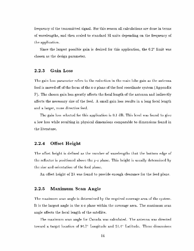
2.4 Feed Location Calculation

Feed locations were calculated to provide uniform coverage of Canada using a 0:2

beam width for a 3 dB beam contour. The beam distortion due to the curvature of

the earth was not considered signicant to the free space loss of the system.

Seventy feeds are required to provide the necessary coverage. The beams are

spaced laterally by approximately 1 . This is sucient distance required for the

feed size calculated in the antenna design section. The beam spacing depends on

the re ector tilt angle and the calculated focal length. The target center for the

satellite was chosen to be 51:4

Latitude, and 94:3

Longitude. This corresponds to

the geographic center of Canada. Plots of the beam coverage area and the distribution

of feeds on the feed plane may be referenced in Figures 2.2, and 2.3.

For the broadband satcom application, the goal of systems with beamforming is

to incorporate a less dense collection of feeds and to dynamically control the array

19

so as to give comparable or better coverage using less hardware as compared to the

single feed per sector design.

−0.4 −0.3 −0.2 −0.1 0 0.1 0.2 0.3 0.4

−0.4

−0.3

−0.2

−0.1

0

0.1

0.2

0.3

0.4

−0.4

−0.2

0

0.2

0.4

Satellite Footprints

Figure 2.2: Satellite Footprint Coverage of Canada, Dimensions in

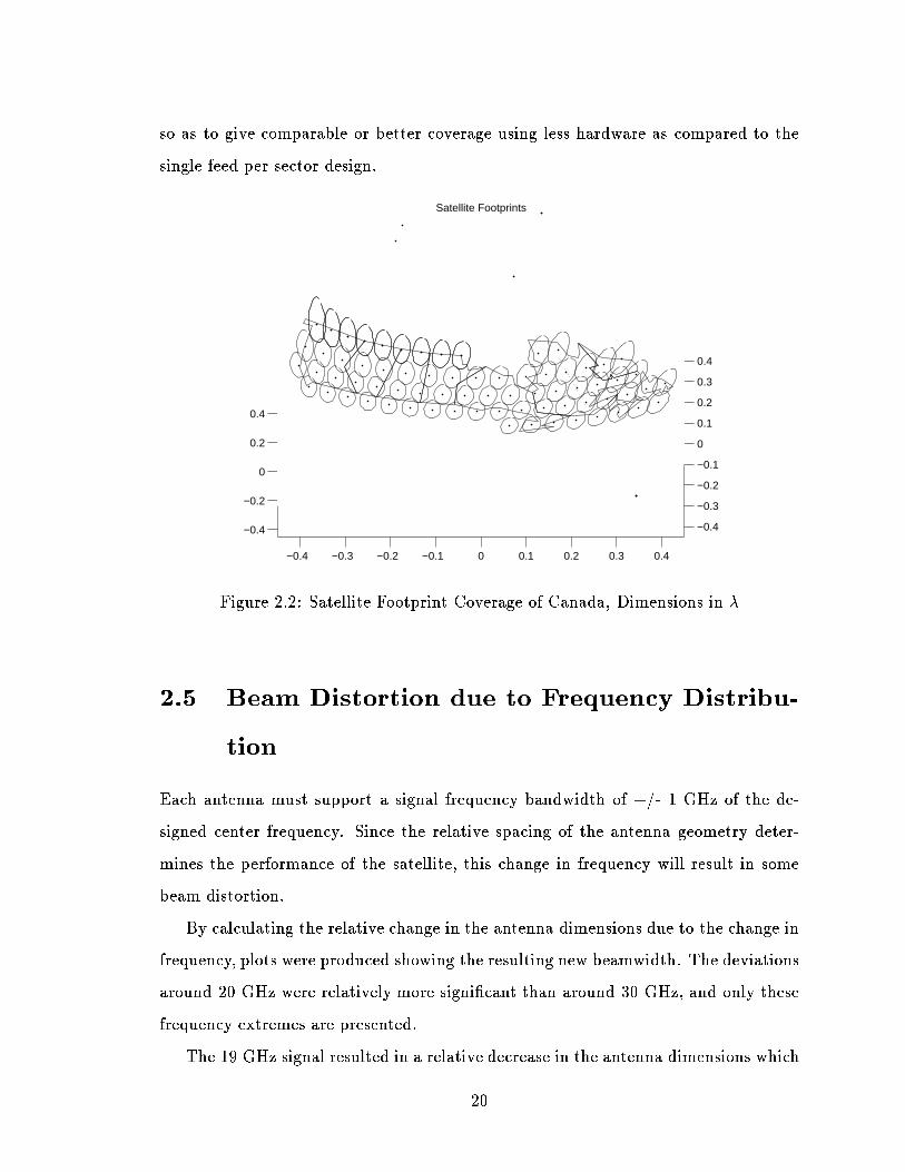
2.5 Beam Distortion due to Frequency Distribu-

tion

Each antenna must support a signal frequency bandwidth of +/- 1 GHz of the de-

signed center frequency. Since the relative spacing of the antenna geometry deter-

mines the performance of the satellite, this change in frequency will result in some

beam distortion.

By calculating the relative change in the antenna dimensions due to the change in

frequency, plots were produced showing the resulting new beamwidth. The deviations

around 20 GHz were relatively more signicant than around 30 GHz, and only these

frequency extremes are presented.

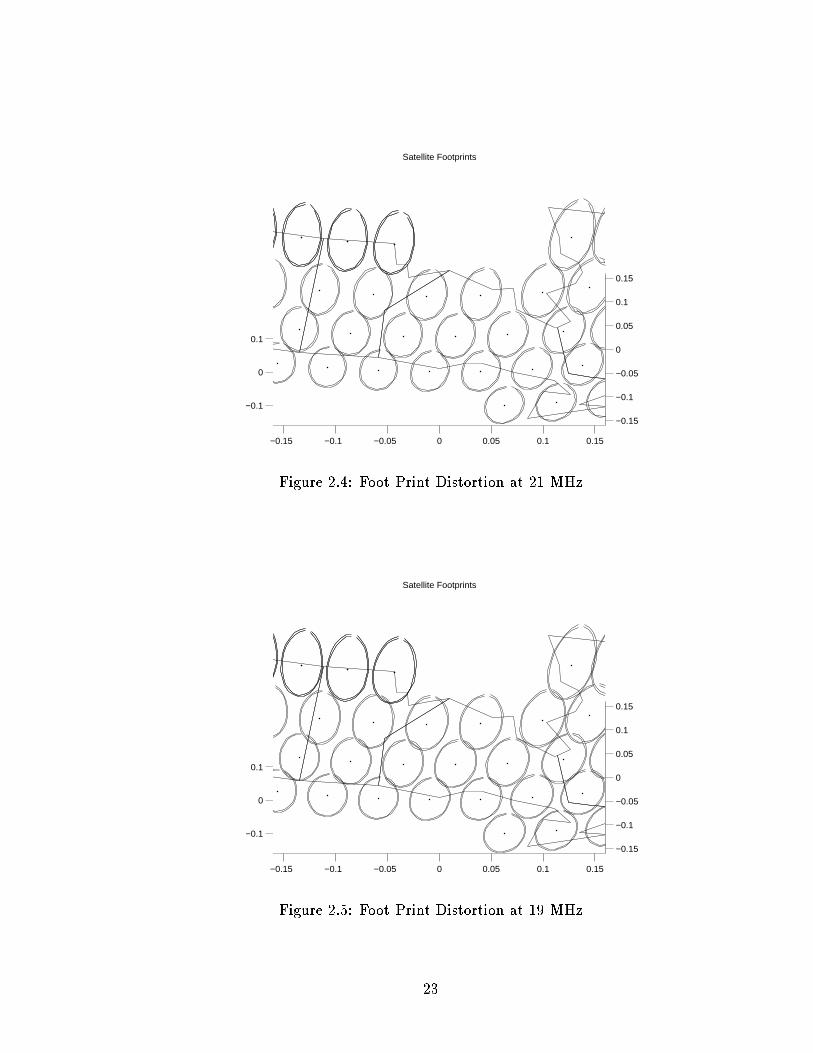
The 19 GHz signal resulted in a relative decrease in the antenna dimensions which

20

−10 −8 −6 −4 −2 0 2 4 6 8−1.5

−1

−0.5

0

0.5

1

1.5

2

Y axis

X a

xis

Feed Coordinates

Figure 2.3: Feed Plane Element Location for Coverage of Canada

21

resulted in a broader beamwidth and a lower gain. In this case the beamwidth in-

creased to 0:22

. Simulation plots showed that this deviation was not signicant.

Conversely, the 21 GHz signal resulted in a relative increase in the antenna dimen-

sions which resulted in a narrower beam width and a higher gain. The beamwidth

decreased to 0:191

Again, simulations showed that the change did not signicantly

aect coverage area or preformance. Plots of the distortion due to frequency of the

beam foot prints may be referenced in Figures 2.4 and 2.5.

The 29 and 31 Ghz signals resulted in a new 3 dB beamwidth of 0:206

and 0:194

respectively. The beam distortion for the coverage area was less than that for the 20

GHz carrier, and was therefore not considered signicant.

Frequency (GHz) Beamwidth (deg)

19 0.211

20 0.200

21 0.191

29 0.206

30 0.200

31 0.194

Table 2.8: Beamwidth Distortion due to Frequency

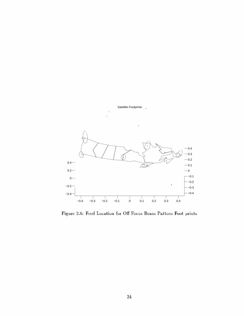
2.6 Degradation in Performance for O Focus Beams

When a feed is displaced from the geometric focus, the resulting electromagnetic eld

no longer arrives at the feed with a coherent phase. This produces a decrease in the

eective gain of the antenna.

Six antenna feed locations were chosen from the feed plane. Five of the feed

locations (1-5) corresponded to beam footprints on the edge of the coverage area. The

6th location corresponded to the focal point of the feed. The program by Duggan

[11] was used to calculate the beam patterns.

22

−0.15 −0.1 −0.05 0 0.05 0.1 0.15

−0.15

−0.1

−0.05

0

0.05

0.1

0.15

−0.1

0

0.1


Figure 2.4: Foot Print Distortion at 21 MHz

−0.15 −0.1 −0.05 0 0.05 0.1 0.15

−0.15

−0.1

−0.05

0

0.05

0.1

0.15

−0.1

0

0.1


Figure 2.5: Foot Print Distortion at 19 MHz

23

−0.4 −0.3 −0.2 −0.1 0 0.1 0.2 0.3 0.4

−0.4

−0.3

−0.2

−0.1

0

0.1

0.2

0.3

0.4

−0.4

−0.2

0

0.2

0.4


Figure 2.6: Feed Location for O Focus Beam Pattern Foot prints

24

It was found that the on-focus feed had the largest gain (53.4 dB), while the worst

gain was from feed number 1 (48.1 dB). This feed location was used in the link budget

calculation as a worst-case scenario.

The coverage area of these feeds and their location on the feed plane may be

referenced in Section 2.6. The corresponding antenna gain patterns for the worst feed

may be referenced in Section 2.7. The optimal on-focus feed may be referenced in

Section 2.8. Remaining plots of the other feed locations are presented in Appendix C

Beam Longitude Latitude x

plane

y

plane

Tilt Max Max

Number (degrees) (degrees) (degrees) dB

1 53 47.5 1.165 -8.869 -0.53 3.696 48.1

2 137 60 -0.976 6.481 0.42 -2.800 49.9

3 126 47.5 0.989 6.985 -0.45 -2.857 49.75

4 80 44 1.557 -3.745 -0.67 1.524 52.1

5 73 60 -1.227 -3.642 0.49 1.451 52.25

6 94.8 51.4 0 0 0.00 0.00 53.4

Table 2.9: Gain and Location Data for Sample Coverage Areas

25

0 0.5 1 1.5 2 2.5 3 3.5 4 4.5 50

10

20

30

40

50

60Magnitude

Deg

Mag

nitu

de in

dB

Figure 2.7: Beam Pattern of Feed 1

0 0.5 1 1.5 2 2.5 3 3.5 4 4.5 50

10

20

30

40

50

60Magnitude

Deg

Mag

nitu

de in

dB

Figure 2.8: Beam Pattern of Feed 6

26

Chapter 3

Link Budget Calculation for the

Ka-Band Geostationary Satellite

Based on the coverage area and the antenna design calculated in Chapter 2, a link

budget was determined for the proposed broadband satellite system operating at the

Ka frequency. This chapter details some of the rst-order eects contributing to the

link budget.

3.1 Ka-Band Link Budget Contributions

The link budget is the calculation of the signal energy in the channel. This budget

determines the number of users that can be supported by the system, and the quality

of service that can be provided.

Figure 3.1 shows the factors in the Link calculations. Only the most signicant

of these factors were incorporated in a rst order Link Budget calculation. The Link

Budget can be calculated using the following formula:

C

N

t

= P

t

+G

Sat

+G

Ea

L 10 log(N

t

) (3.1)

27

stratificationelectron densitysolar flares

ice crystalshumidity

ionosphericeffects

Faraday rotation

phae/range errors

scintillation

ice crystalsdustsnowhailsleetrain

raindepolarisation

depolarisationice crystal

troposphericclear-sky effects

scintillationmultipath ray bendinggaseous attention

transmitted signal

CLEAR SKY

DEGRADED SKY

attenuation

scatter

absorption

Figure 3.1: Diagram of Atmospheric Eects on the Channel

28

C=N ) Carrier to noise power ratio (dBm)

P

t

) Power transmitted (mW)

G

Sat

) Satellite Antenna Gain (dB)

G

Ea

) Earth Antenna Gain (dB)

L ) Total Loss (dB)

N

t

) Thermal Noise (dB)

The remainder of this section provides a summary of the calculation of the pa-

rameters, and a comparison with values from literature.

3.1.1 Physical Link Parameter Summary

To begin the calculation of the link budget several parameters must be determined

including frequency, link direction, satellite position, and target location.

The system is to be operated in the Ka frequency range (20-30 GHz). This band is

presently unallocated, and can provide the necessary bandwidth. The frequencies near

22 GHz were avoided for this system because these values were close to the resonant

frequency of water (Section D.6). This resonance would cause a large amount of signal

attenuation.

Specifying up/down link directions in the calculation are needed to determine

the worst path. In general, atmospheric attenuation increases with the increase of

frequency. Furthermore the thermal noise in each link is also dierent due to the

Downlink Degradation factor (section D.9). As a result, one link direction will be

more attenuated than the other. Attenuation may be compensated from the earth

station using an increase of transmit power or by more complex receiver or antenna

design. A satellite system would typically not have these resources due to payload

and power limitations. Based on this reasoning, the downlink was given the lower

frequency band (20 GHz).

The geometry of the link is determined by the satellite and the earth latitude and

longitude coordinates. Typically, coverage will not be guaranteed for target locations

greater than 70

latitude. Points at this latitude have an elevation angle below 10

.

29

Attenuation increases greatly at these latitudes (Section D.6.3).

3.1.2 Earth/Satellite EIRP

The Equivalent Isotropic Radiated Power (EIRP) for the earth and the satellite are

calculated using the following formulas:

EIRP = G

t

+ P

t

(3.2)

where G

t

is the transmitter antenna gain, and P

t

is the transmitter power.

The typical antenna gain values found in literature for existing Ka and Ku band

satellites ranges from 25 - 45 dB. This gain is given by:

G

t

=

4(A

A

s

o

i

)

2

(3.3)

A

A

) Antenna aperture (m

2

)

G

t

) Transmitter antenna gain (dB)

P

t

) Transmitter power (dBW)

s

) Spill-over eciency

o

) Manufacturing eciency

i

) Illumination eciency

) Wavelength (m)

In addition, the antenna eciency is decreased by non-ideal properties such as

surface blemishes, however the limiting factor in eciency for a multi-beam antenna

is due to the Stein Limit which is 50 % [10] (Section A.5.1).

The maximum gain that could be achieved while giving reasonable re ector di-

mensions and coverage footprints was 53.4 dB for on focus feed. Gains above this

resulted in very large antennas, with very small beam footprints which would require

many feeds to cover the desired geographic area.

30

3.1.3 Free Space Loss

The free space loss is the loss due to the distance that the transmitted signal must

travel through free space. This is found using the following formula:

L

fs

= (

4r

)

2

(3.4)

Where r is the radius from the source. The radius is determined by the satellite

and target coordinates. This loss was found to be the largest single contributor to

signal attenuation. The large distances required for Geostationary orbit which result

in high free space losses are one of the major drawbacks of this system.

3.1.4 Gaseous Losses

The calculations of the gaseous losses are done based on the CCIR model presented

in [3] (Section D.6). These losses are not signicant at lower frequencies, but in the

Ka band they should be considered. The major gases which contribute to attenu-

ation are oxygen and water. The CCIR model [3] is used to calculate the gaseous

attenuation of the system. Water has a resonance frequency at approximately 22

GHz which makes this frequency undesirable. Water attenuation depends largely on

the atmospheric conditions specied by temperature, atmospheric water vapor, and

precipitation conditions. A value of 7 g/m

3

was used as quoted from [3] for the wa-

ter vapor. Correction constants were used in the attenuation formulas to correct for

temperature ranges. Two dierent constants were used in determining the equivalent

atmospheric height of water vapor for rainy and clear sky conditions. The resonant

frequency of Oxygen is at approximately 60 GHz. This frequency is well outside of

the bandwidth being investigated. A detailed calculation of Oxygen attenuation is

presented in Appendix D

31

3.1.5 Rain Attenuation

The rain attenuation model used was the CCIR model (Section D.8). The values gen-

erated using this method have been shown to have a good correlation with measured

values [3] while requiring a minimal amount of statistical data. The CCIR divides

the world into dierent regions based on rain fall statistics. Canada falls mainly in

regions E and C. Region E was chosen for determining the rainfall model as a pes-

simistic parameter. This rainfall area has a precipitation rate exceeding 22 mm/h for

0.01 % of the year [3].

3.1.6 Temperature

Several dierent temperatures are signicant in the calculation of the system temper-

ature. These include the receiver temperature, the cosmic temperature, the ground

temperature and the medium temperature. The direction of the link is also impor-

tant. In the downlink, the earth station sees cool sky. As the signal passes through

the atmosphere, some of the energy of the signal is absorbed and retransmitted as

thermal noise. This eect is quantied in the downlink degradation factor (section

D.9) which has been shown to increase the attenuation by as much as 2 dB.

3.1.7 Bandwidth Calculation

The bandwidth section of the link calculation provides information which is specic to

the type of system proposed. This includes the uplink and downlink band frequency,

the information bandwidth, the size of the guard bands and the type of pulse used.

This information gives a bit energy over signal and noise ratio. Depending on the

modulation scheme used, this would correspond to a particular bit error rate as well

as the number of channels available.

32

3.2 FDMA System

This system has the basic conguration that will be used as a baseline for comparison

with other beamforming systems. The FDMA scenario has no beamforming. The

down link is considered the most critical direction due to the limitations of satellite

power, mass and receiver complexity. The system is noise limited. This is a result of

the large amount of attenuation on both desired and interference signals, and from

the frequency separation of signals which allows for front- end ltering. Interferers

from other systems at the Ka band are not anticipated in the signal environment.

The statistical models on which the link budget has been based show that the

channel is slowly time varying. Experimental results from [27] support the slowly

time varying model.

Each user is assigned a unique frequency for the uplink and the downlink. The

link budget for this system shows the major losses in the link and the amount of

additional gain that would be required due to channel coding and beamforming to

make the system feasible. The system is compared with the link analysis performed

by Karimi for a low bit rate (9600 bps) voice system operating at L-band [21].

A more detailed explanation of the link budget calculations is presented in the

following sections.

3.3 Link Budget Calculation

The link budget is a calculation which shows the expected carrier to noise ratio of

the system under the specied conditions. This ratio is directly related to the E

b

=N

o

[3]. From this calculation a prediction of the bit error rate and the reliability of of

service can be determined.

The following sections outline the values chosen for the input parameters and the

calculations which result.

33

3.3.1 Hardware Specications

Hardware losses for both the uplink and the downlink were estimated at 2.0 dB for

the each receiver and 0.2 dB for each feed. These were the values presented in [3].

The satellite gain was calculated using the designed parabolic antenna presented in

the previous section. The power for each downlink signal was limited to 1 Watt due

to power constraints on the satellite.

The earth antenna gain was set at 0 dB and the earth transmitter was given a

power of 1 Watt. In this way the design of the satellite system alone can be evaluated

and the necessary gain needed from the earth station to make the system feasible can

be determined.

3.3.2 Frequency Parameters

Frequencies in the Ka frequency band were chosen because this band has not yet been

allocated. There is a large amount of available bandwidth which could support high

data rate services.

Frequency has a direct eect on the power of the received signal due to rain

attenuation and free space loss. Free space loss increases at a rate of inverse distance

squared. The frequency scaling method presented by [25] (section D.10) was used for

frequencies +/- 1 GHz for the up and downlink frequencies of 30 and 20 GHz.

3.3.3 Target Latitude and Longitude

The target latitude and longitude were selected based on the coverage area of the

feed with the worse gain as calculated in the antenna design section (Feed # 1).

The geographical coordinates of feed # 1 correspond to 47:5

Latitude and 53:0

Longitude. The satellite Latitude position must be situated on the equator 0

in

order to maintain a geostationary position. The Longitude position of the satellite

was chosen to be 94:7

which is the geographic center of the coverage area.

34

3.3.4 Height above Sea Level

A target's height above sea level aects the attenuation due to the free space loss,

as well as the eect of rain on the slant path of the signal. A height of 0.2 km was

selected for the elevation of the target.

3.3.5 Outage Percentage

The outage percentage is a statistical calculation which is used to predict the per-

centage of time that atmospheric attenuation exceeds a certain threshold (Section

D.8). This calculation is based on the CCIR attenuation model as presented in [3].

The model is dependent on the geographic parameters as well as the frequency of the

signal.

An outage percent probability of 0.01 % was used for this system. The 0.01%

level is the value derived from measured systems. Other percent outage levels must

be calculated indirectly using a scaling method.

The 0.01 % level gives a statistical prediction that the attenuation due to rain will

exceed the calculated threshold only 0.01 % of the year.

3.3.6 Antenna Gain Reduction

For an antenna design having a beam width of 0:2

and servicing a location having

an elevation angle of 20

the antenna gain reduction was found to be 0.5 dB [3].

3.3.7 System Interference

In the FDMA system, no interference from other users was modeled. This is due to

the fact that all users occupy a unique frequency and from the fact that channels

are spaced with 1 Mhz guard bands at the upper and lower edges of each channel.

Broadband front-end ltering would provide additional attenuation to interfering sig-

nals. The narrow beamwidth of the antenna and low side lobe levels tend make user

signals in other geographic areas very weak relative to the desired signal. For this

35

reason, the FDMA system is seen to be noise-limited. Further justication for this

assumption is presented through simulations in Chapter 7.

3.3.8 Temperature Parameters

Summer temperatures were estimated for the system to give a worst-case scenario.

Temperatures were selected based on those found in literature and through personal

communication with system designers. The selected parameters are presented in chart

form in the link analysis summary.

The temperature values chosen signicantly aect the amount of attenuation

which results from the downlink degradation factor (Section D.9).

8 MHz 1 MHz1 MHz

10 MHz

19 GHz 20 GHz 21 GHz 29 GHz 30 GHz

Figure 3.2: Allocation of Channels at the Ka Band

3.3.9 Channel Guard Bands

In order to decrease the interference from other users, guard bands of 1 MHz are

placed between each channel. A schematic of the frequency allocation is given in

gure 3.2.

36

3.3.10 Pulse Design

A binary phase shift keying pulse was used to transmit data. This scheme simplies

the recovery of the message signal at the receiver.

To minimize intersymbol interference a 100 % raised cosine pulse was selected.

This eectively doubles the bandwidth of the system. The increase in bandwidth is

not seen as a problem due to the large amount of unallocated bandwidth in the Ka

band.

3.3.11 Base Band Channel

The basic information rate was selected for 2 Mbps. The 2 Mbps rate will allow for

high data rate transfer as well as image transmission.

3.3.12 Ionospheric Eects

The major parameter controlling the eect of the the ionosphere are the Total Electron

Count (TEC=#=m

3

) and the frequency. The TEC value of 10

17

was used [3]. The

ionospheric eects are not seen as signicant with respect to signal distortion. The

reason for the small in uence of the ionosphere on the signal is due to the inverse

frequency dependence on the degradation parameters. A detailed description of the

ionospheric eects are presented in Appendix D. The ionospheric eects were not

considered further.

3.3.13 E

b

=N

o

Requirements

The E

b

=N

o

level was selected to give a Bit error rate (BER) of 10

5

for binary phase

shift keying pulses. This level corresponds to an E

b

=N

o

of 10 [40]. Additional gain

from beamforming and coding would be expected to increase this level to give data

quality performance of 10

6

or better.

37

Satellite Rx Loss (dB) 2

Satellite Feed Loss (dB) 0.2

Satellite Gain (dB) 48

Satellite Power (dBW) 0

Earth Rx Loss (dB) 2

Earth Feed Loss (dB) 0.2

Earth Gain (dB) 0

Earth Power (dBW) 0

Target Latitude (deg) 47.5

Target Longitude (deg) 53.0

Satellite Longitude (deg) 94.8

Earth Feed Temp (

K 300

Sat Feed Temp (

K) 200

Earth Temp (

K) 300

Sat Temp (

K) 200

Sky Temp (

K) 2

Medium Temp (

K) 290

Ground Temp (

K) 300

Guard Band (MHz) 1

Base Band (MHz) 2

Raised Cosine % 100

TEC (#/m

2

) 10

17

Height above Sea (km) 0.2

Outage (%) 0.01

Aperture Degradation (dB) 0.5

Interference Noise (dB) 0.0

H

2

O Vapor (), (g/m

3

) 7.0

Table 3.1: Link Budget Parameters: FDMA System

38

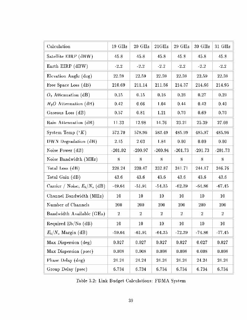
Calculation 19 GHz 20 GHz 21GHz 29 GHz 30 GHz 31 GHz

Satellite EIRP (dBW) 45.8 45.8 45.8 45.8 45.8 45.8

Earth EIRP (dBW) -2.2 -2.2 -2.2 -2.2 -2.2 -2.2

Elevation Angle (deg) 22.59 22.59 22.59 22.59 22.59 22.59

Free Space Loss (dB) 210.69 211.14 211.56 214.37 214.66 214.95

O

2

Attenuation (dB) 0.15 0.15 0.16 0.26 0.27 0.29

H

2

O Attenuation (dB) 0.42 0.66 1.04 0.44 0.42 0.40

Gaseous Loss (dB) 0.57 0.81 1.21 0.70 0.69 0.70

Rain Attenuation (dB) 11.33 12.98 14.76 23.21 25.39 27.69

System Temp (

K) 572.70 578.96 583.49 485.99 485.97 485.96

DWN Degradation (dB) 2.15 2.03 1.84 0.00 0.00 0.00

Noise Power (dB) -201.02 -200.97 -200.94 -201.73 -201.73 -201.73

Noise Bandwidth (MHz) 8 8 8 8 8 8

Total Loss (dB) 228.24 230.47 232.87 241.71 244.17 246.76

Total Gain (dB) 43.6 43.6 43.6 43.6 43.6 43.6

Carrier / Noise, E

b

=N

o

(dB) -49.64 -51.91 -54.35 -62.39 -64.86 -67.45

Channel Bandwidth (MHz) 10 10 10 10 10 10

Number of Channels 200 200 200 200 200 200

Bandwidth Available (GHz) 2 2 2 2 2 2

Required Eb/No (dB) 10 10 10 10 10 10

E

b

=N

o

Margin (dB) -59.64 -61.91 -64.35 -72.39 -74.86 -77.45

Max Dispersion (deg) 0.027 0.027 0.027 0.027 0.027 0.027

Max Dispersion (psec) 0.008 0.008 0.008 0.008 0.008 0.008

Phase Delay (deg) 24.24 24.24 24.24 24.24 24.24 24.24

Group Delay (psec) 6.734 6.734 6.734 6.734 6.734 6.734

Table 3.2: Link Budget Calculations: FDMA System

39

3.4 Comparison with L Band Voice System

There is signicantly more loss resulting in the broadband scenario proposed as com-

pared to voice band systems which operate at lower frequencies. In order to illustrate

the source of these dierences, a comparison was made with the 9.6 kbps voice band

system proposed by [21].

Parameter 1.6 GHz 30 GHz Dierence

Bit Rate 9.6 kbps 2 Mbps

Free Space Loss (dB) 188.38 214.66 26.28

Noise Power (dB) -158.34 -141.73 22.61

Weather Attenuation (dB) 0.1 26.08 25.98

Total Major Attenuation Factors (dB) 30.14 105.01 74.87

Table 3.3: Up Link Performance Comparison:Ka System with L Band System

Parameter 2.0 GHz 20 GHz Dierence

Bit Rate 9.6 kbps 2 Mps

Free Space Loss (dB) 190.11 211.14 21.03

Noise Power (dB) -157.11 -140.96 22.15

Weather Attenuation (dB) 0.1 13.79 13.69

Total Major Attenuation Factors (dB) 33.1 89.97 56.87

Table 3.4: Down Link Performance Comparison:Ka System with L Band System

As this analysis shows that the major factors contributing to the system attenua-

tion as compared to the lower frequency and data rate system are the free space loss,

the noise power (which is a function of the data rate and noise power bandwidth) and

the attenuation due to weather.

The values aecting the magnitude of this attenuation are the result of the desired

frequency band the of the service required. Practical receiving antennas are limited

40

to a gain of approximately 50 dB due to size constraints, construction and pointing

errors. It is anticipated that beamforming will allow for an increase in the signal to

noise ratio which would make this system less costly.

41

Chapter 4

Cyclostationary Beamforming and

On-Board Processing

The underlying principles behind the cyclostationary beamforming techniques, and a

summary of existing cyclostationary algorithms will be presented.

A brief summary of the advantages of beamforming and on board processing will

be discussed, and the advantages of cyclostationary algorithms over other beamform-

ing techniques will be summarized.

4.1 Motivation for Digital Beamforming and On-

Board Processing

On-Board Processing deals with the general topic of improving the received signal of

the system in question before it is retransmitted to the desired user. Three forms of

on-board processing take the form of regenerative repeaters, adaptive power control,

and antenna beamforming.

This thesis will investigate the area of digital beamforming method of on-board

processing as applied to the geostationary satellite mobile communications environ-

ment at the Ka frequency band. Digital Beamforming can oer the following advan-

tages in a communications environment:

42

Adaptive beams may be dedicated to individual users using antenna arrays.

Power can be eciently focused on a target area to improve the satellite system's

eciency.

The beamforming array can adapt to variations in the user trac levels

The increased eciency of power usage could translate into reduced hardware

requirements and payload expense.

Frequency reuse may be increased as a result of narrower adaptive beams which

reduce interference from adjacent channels.

Beamforming may oer robustness to the system in the event of component

failure.

There are three general methods of beamforming being actively investigated in the

present literature. The following sections brie y introduce the basic principles of these

methods, and relate their application to the satellite system under investigation. For

a more complete account of beamforming, tutorial papers by Van Veen and Buckley

[41] and the text by Monzingo and Miller [28] may be referenced.

4.1.1 Reference-Based Beamforming

In reference based beamforming, a know signal which is highly correlated with the

desired data and uncorrelated with interference signals is transmitted. This reference

signal often takes the form of a known transmitted training sequence. Beamforming

weights are calculated based on the reference signal using a variety of algorithms, the

most common of which are Least Mean Square, and Direct Matrix Inversion. The ma-

jor drawback of the reference-based beamforming method is the power and bandwidth

resources that are taken up by the reference signal. In the satellite environment, this

power cost is highly undesirable.

43

4.1.2 Location-Based Beamforming

Location-based beamforming relies on knowledge of the direction of arrival of the

desired signal and the interference signals. Using this information, optimum beam

weights may be calculated to suppress the interference, and boost the desired signal.

This technique relies on algorithms which reliably estimate the direction of both

the desired and interference signals. This is often done on the basis of eigen-vector

analysis, such as the Multiple Signal Classication algorithm (MUSIC) [36] Most

of these direction estimation algorithms require accurate knowledge of the type of

interference, and the geometry of the array manifold.

In the portable satellite communications environment, weather patterns are con-

stantly changing, and the ability to characterize the system once deployed is dicult.

These disadvantages would make knowledge of the interference environment dicult,

and the array geometry calibration less robust.

4.1.3 Property Restoral/Blind Beamforming

The property restoral beamforming technique focuses on maximizing inherent prop-

erties of the desired signal which are already present during transmission. Typically

these characteristic signal properties are degraded by noise and interference. Algo-

rithms are employed which beamform to restore these properties in the signal. It is

assumed that by restoring the characteristic properties, the entire message signal is

improved. Two techniques of property restoral are the Constant Modulus algorithm

[37], and Cyclostationary Property Restoral technique [2].

The most obvious advantage of this type of beamforming is that there is no need

for a reference signal, or accurate knowledge of the interference environment. Only

accurate knowledge of the property to be restored is needed.

44

4.2 Motivation for the Cyclostationary Property

Restoral Technique

Cyclostationary theory and techniques have been pioneered in various works by Gard-

ner [16] [14]. Cyclostationarity exploits the behavior that most man-made signals

exhibit a high degree of correlation with characteristic frequency shifted versions of

themselves. Through selected weighting and summing of the signal at these frequen-

cies, the cyclic correlation coecient can be calculated. This coecient is a measure

of the similarity between the received signal and the frequency shifted signal. By ad-

justing antenna element weight coecients to maximize this property, beamforming

can be done to improve the reception of the entire message signal.

The advantages which result from the cyclostationary method are many. The

beamforming algorithms are blind. They require no knowledge of the transmitted

waveform. No training signal is needed and no knowledge of the noise and inter-

ference statistics are necessary. It is not necessary to calibrate the algorithm with

measurements of the array manifold. The cyclostationary algorithms do not increase

bandwidth or power requirements of the signal, and no synchronization is needed with

the transmitter, which is a highly prohibitive requirement for the long distances and

time delays involved in satellite communication. The only knowledge that is needed

is the cyclic frequency of the chosen signal to be restored.

The major drawback of the cyclostationary algorithms are their high computa-

tional requirements and their slow convergence rate. Present literature has focused

mainly on developing computationally ecient algorithms in SINR environments in

the range of 0 to 20 dB [34] [2]. The focus of investigation for this thesis is on mod-

ifying existing algorithms to work in the geostationary satellite environment at the

Ka band where SINR levels may be as low as -110 dB (Table 3.2) without antenna

gains.

45

4.3 Theoretical Background for Cyclostationary

Analysis

The theory of Cyclostationary analysis rst began to receive attention in 1972 with

Gardner's PhD. thesis [14]. Over the past 25 years, his original presentation which fo-

cused on real time series properties of cyclostationarity, has been extended to include

complex time series and has been linked with statistical theory. Areas of application

for cyclostationarity are being developed in the areas of array processing, transmit-

ter/receiver optimization, blind channel equalization and identication.

Cyclostationarity exists in a signal if and only if a nite amplitude sine wave is

produced when the original signal is multiplied by a non-linear n-th order transforma-

tion. This is calculated through temporal processing. A signal, x(t), exhibits second

order (n=2) cyclostationarity at the cyclic frequency if and only if its delay product

waveform, y(t), exhibits a spectral line at this frequency.

y(t) = x(t)x(t ) (4.1)

Higher order non-linearities with a multiple lag parameters (ie.

1

;

2

; :::) will

generate spectral lines for higher order cyclostationary time series. For wide sense

stationary signals, a spectral line is only observed for the case = 0.

The cyclic spectrum is dened as all cyclic frequencies where the signal exhibits

a spectral line. Cyclic spectrums of man-made signals are often unique. Therefore,

the unique cyclic spectrum of the desired signal may be exploited resulting in the

rejection of noise and interferers, and enhancement of the desired signal.

Processing of the cyclostationary spectrum is done using time series analysis. As

a result, the desired signal must be ergodic in nature, which will allow the ensemble

average to equal the time average in the limit as the averaging time goes to innity.

Fortunately, most communications signals and environments are ergodic in nature.

The next section presents a brief outline of the theory and motivation behind

cyclostationarity. Many of the results are presented without proof or justied by

46

appeal to the analogous well known property in a stochastic environment.

The cyclic theory presented by Gardner is based on the extension of Wiener's time-

series analysis to cyclostationary signals of arbitrary order. Using this approach, tem-

poral and spectral moments, higher order moments, bias, variance and Cramer-Rao

bounds may be calculated. The application to this thesis is to provide a theoretical

justication for the second order cyclostationary equations used in the beamforming

algorithms applied. A full presentation of the following theory may be referenced in

[16]. The "^" notation is used to distinguish between time-series measures and the

related probabilistic measures.

4.3.1 Fraction of Time Probability Measure

Let the event indicator be dened as

I[x x(t)]

4

=

8

>

<

>

:

1; x(t) < x

0; x(t) > x

(4.2)

The time averaging of the event indicator results in the fraction-of-time probability

distribution.

^

F

0

x(t)

4

=

^

E

0

fI[x x(t)]g (4.3)

Where the time-averaging operator

^

E

0

is dened as:

^

E

0

fh(t)g

4

= lim

Z!1

1

2Z

Z

Z

Z

h(t+ t

0

)dt

0

(4.4)

Where h(t) is any time dependent signal.

The joint fraction-of-time probability distribution may be generalized for the set

of variables x

4

= fx(t+ t

1

); x(t+ t

2

); :::x(t+ t

n

)g

^

F

0

x(t)

4

=

^

E

0

f

n

Y

j=1

I[x

j

x(t+ t

j

)]g (4.5)

47

The joint fraction of time probability density which results when (4.5) is dieren-

tiable.

^

f

0

x(t)

(x) =

@

n

@x

1

; @x

2

; :::@x

n

^

F

0

x(t)

(x) (4.6)

The following theorem results from the Fraction-of-Time formulation of the time

signal x, which is based upon the parallel stochastic process principle, the "Funda-

mental Theorem of Expectation". It states:

Theorem 1 (Fundamental Theorem of Time-Averaging)

For every time-invariant function g() for which

^

E

0

fg[x(t)]g exists,

^

E

0

fg[x(t)]g =

Z

g(x)

^

f

0

x(t)

(x)dx (4.7)

This theorem shows that the time averaging operator

^

E

0

fg can be thought of as

the temporal expectation operator. It may also be shown [34] that the

^

E

0

fg may

remove residual terms in the time-averaged equation. Therefore

^

E

0

fg is also referred

to as the constant component extractor.

In the probabilistic environment, the joint density of a cyclostationary stationary

process is periodic in t. Similarly the Fraction-of-time probability density function is

also periodic in t. In order to extend the principle of the constant component extractor

to a polyperiodic function, consider the time series Fraction-of- Time probability

density

^

F

0

x(t)

(x) which is a polyperiodic function of t. This function can be expanded

in a Fourier series as

^

F

0

x(t)

x(t) =

X

^

F

0

x(0)

(x)e

i2t

(4.8)

=

X

^

F

x(t)

(x) (4.9)

Here

^

F

x(0)

(x) are the Fourier series coecients, and denotes the cyclic frequency.

The sinusoidal components of

^

F

x(t)

(x) may be given by:

48

^

F

x(t)

(x)

4

=

lim

Z !1

1

2Z

Z

Z

Z

^

F

0

t+t

0

(x)e

i2t

0

dt

0

(4.10)

=

^

E

0

f

^

F

0

x(t)

(x)e

i2t

0

ge

i2t

0

(4.11)

4

=

^

E

f

^

F

0

x(t)

g (4.12)

The general sinewave component extractor may be written as:

^

E

fg

4

=

^

E

0

f()e

i2t

ge

i2t

(4.13)

Using this denition of the sinewave component extractor, the multiple periodic-

ities of a time series may be extracted by:

^

E

fg

4

=

X

2fg

^

E

fg (4.14)

The set of fg frequencies which are extracted represent the harmonics of the re-

ciprocals of the underlying multiple periodicities in the signal. Finally, the expression

for the polyperiodic Fraction-of-Time Probability distribution for a time-series with

multiple periodicities becomes:

^

F

x(t)

4

=

^

E

f

n

Y

j=1

I[x

j

x(t+ t

j

)]g (4.15)

The polyperiodic Function of Time density which results is:

^

f

x(t)

(x) =

@

n

@x

1

; @x

2

; :::@x

n

^

F

x(t)

(x) (4.16)

Theorem 2 (Fundamental Theorem of Polyperiodic Component Extrac-

tion)

For every time-invariant function g() for which

^

E

fg[x(t)]g exists:

^

E

fg[x(t)]g =

Z

g(x)

^

f

x(t)

(x)dx (4.17)

49

The strict sense denitions of cyclostationarity follow from the preceding theorem.

Dene fg to be the set of all cycle frequencies for which

^

F

x(t)

6= 0 [34].

Stationarity: A time series x(t) is stationary if and only if its joint fraction of

time probability density

^

F

x(t)

6= 0 exists and is independent of the parameter t. In

this case fg = f0g

Cyclostationarity: A time-series x(t) is cyclostationary with period T

0

if and

only if its fraction of time probability density

^

F

x(t)

6= 0 exists, and is periodic in t

with period T

o

. In this case, the cyclic spectrum fg is composed of all harmonics of

1=T

0

.

Polycyclostationarity: A time-series x(t) is cyclostationary with period T

0

; T

1

; T

2

:::

if and only if its fraction of time probability density

^

F

x(t)

6= 0 exists, and is polyper-

iodic in t with periods T

0

; T

1

; T

2

; ::: In this case, the cyclic spectrum is the set of all

the harmonics of each fundamental period.

The following section will build upon the theorems and denitions presented as

applied to second order cyclostationary time-series.

4.4 Second-Order Cyclostationariy

The second order polyperiodic cyclostationary waveform can be generated as follows:

y

(t) = x(t+ =2)x(t =2) (4.18)

From the theorems and denitions presented in Section 4.3 , the following terms

are obtained from the polyperiodic component extractor

~

E

fy

r

(t)g =

X

fg

~

E

0

fy

r

(t)e

i2t

ge

i2t

(4.19)

=

X

fg

~

R

xx

( )e

i2(t=2)

(4.20)

Here the notation refers to continuous time series, and the omission of this

symbol refers to discrete time series.

50

In Equation (4.20)

~

R

xx

( )

4

= E

0

fx(t+ =2)x(t =2)e

i2t

g (4.21)

is the Fourier series coecient of the additive sine-wave component of y

r

(t) with

frequency . For the discrete case this formula is modied to:

R

xx

( )

4

= E

0

fx(t)x(t )e

i2t

ge

i2

(4.22)

It is important to stress that the above quantities are time-averaged. The constant

component extraction operation will be dened as:

hi

1

= lim

Z!1

1

2Z

Z

Z

Z

()dt (4.23)

For the discrete case the formula is modied to:

hi

1

= lim

Z!1

1

2Z + 1

+Z

X

Z

() (4.24)

4.4.1 Cyclic Autocorrelation Function

The quantity

~

R

xx

( ) may be interpreted in three ways which oer insight into the

measure produced.

1

~

R

xx

( ) may be interpreted as the Fourier coecients of the additive sine-

wave components of the delay product waveform of x(t)x(t ). This was

shown in section 4.3.

2 The conventional autocorrelation function

R

0

xx

( ) = hx(t)x(t )i

1

(4.25)

51

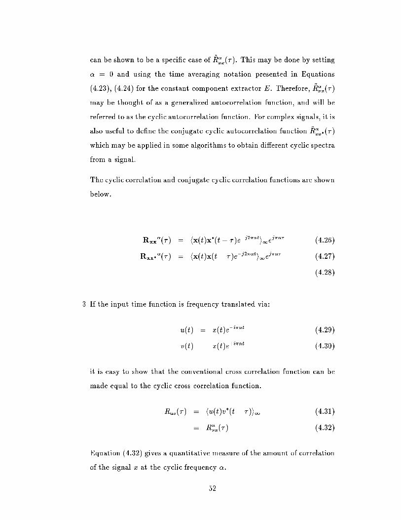
can be shown to be a specic case of

~

R

xx

( ). This may be done by setting

= 0 and using the time averaging notation presented in Equations

(4.23), (4.24) for the constant component extractor E. Therefore,

~

R

xx

( )

may be thought of as a generalized autocorrelation function, and will be

referred to as the cyclic autocorrelation function. For complex signals, it is

also useful to dene the conjugate cyclic autocorrelation function

~

R

xx

( )

which may be applied in some algorithms to obtain dierent cyclic spectra

from a signal.

The cyclic correlation and conjugate cyclic correlation functions are shown

below.

R

xx

( ) = hx(t)x

(t )e

j2t

i

1

e

j

(4.26)

R

xx

( ) = hx(t)x(t )e

j2t

i

1

e

j

(4.27)

(4.28)

3 If the input time function is frequency translated via:

u(t) = x(t)e

it

(4.29)

v(t) = x(t)e

+it

(4.30)

it is easy to show that the conventional cross-correlation function can be

made equal to the cyclic cross correlation function.

R

uv

( ) = hu(t)v

(t )i

1

(4.31)

= R

xx

( ) (4.32)

Equation (4.32) gives a quantitative measure of the amount of correlation

of the signal x at the cyclic frequency .

52

4.5 Cyclic Temporal Correlation Coecient

The cyclic temporal autocorrelation coecient may be generated by normalizing the

the cyclic autocorrelation function with respect to the autocorrelation function of x(t)

for the time lag = 0. This produces the cyclic temporal correlation coecient.

xx

( )

4

=

R

xx

()

R

xx

(0)

(4.33)

The feature strength is dened as the magnitude of equation (4.33)

The value of (4.33) is 0

xx

( ) 1. This quantity is the measure that is

maximized in the existing cyclic correlation algorithms. It should be noted that

(4.33) is complex-valued. Therefore its argument can be used to distinguish between

dierent signals of the same magnitude which may allow algorithms to select signals

with the same cyclic frequencies arriving from dierent directions.

Similarly the cyclic temporal cross correlation coecient may be generated for

two time sequences x(t) and y(t) by:

xy

( )

4

=

R

xy

()

R

xy

(0)

(4.34)

4.6 Spectral Correlation Density Function

Gardner in [17] has related the time domain performance of the cyclic correlation

coecient to the frequency domain. This is be done by passing the frequency trans-

lated signals u(t) and v(t) through an ideal bandpass lter at the center frequency

f . The average power is measured at the output, and the result is normalized by the

bandwidth. This results in the spectral correlation density function:

S

xx

4

=

lim

B ! 0

1

B

Dh

h

f

B

(t) u(t)][h

f

B

(t) v(t)

i

E

(4.35)

where denotes convolution and h

f

B

is the ideal bandpass lter.

53

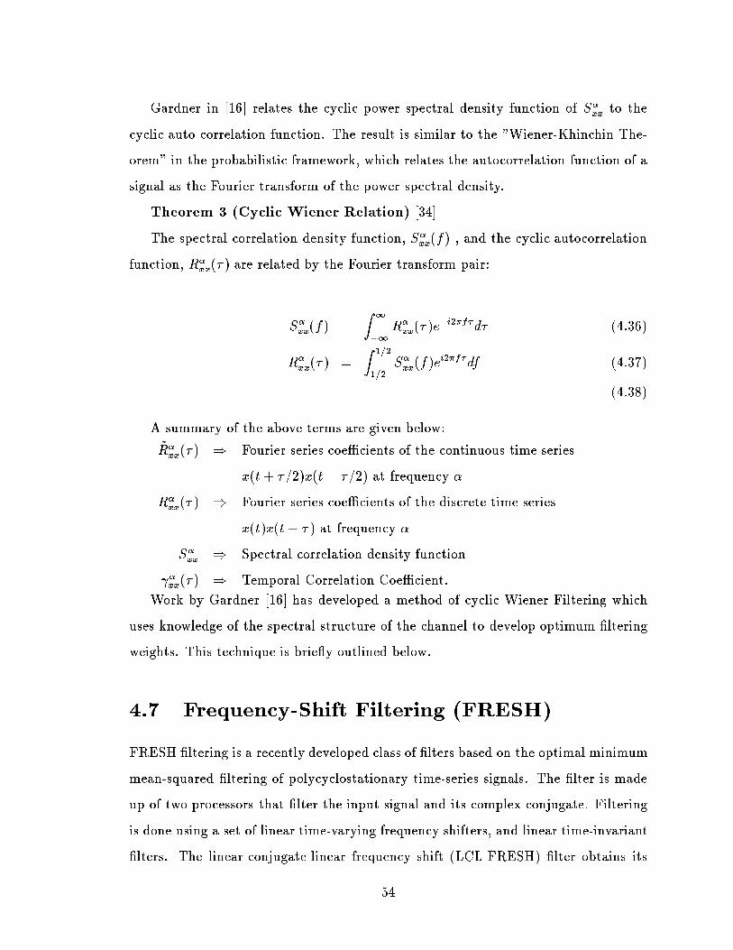
Gardner in [16] relates the cyclic power spectral density function of S

xx

to the

cyclic auto correlation function. The result is similar to the "Wiener-Khinchin The-

orem" in the probabilistic framework, which relates the autocorrelation function of a

signal as the Fourier transform of the power spectral density.

Theorem 3 (Cyclic Wiener Relation) [34]

The spectral correlation density function, S

xx

(f) , and the cyclic autocorrelation

function, R

xx

( ) are related by the Fourier transform pair:

S

xx

(f) =

Z

1

1

R

xx

( )e

i2f

d (4.36)

R

xx

( ) =

Z

1=2

1=2

S

xx

(f)e

i2f

df (4.37)

(4.38)

A summary of the above terms are given below:

~

R

xx

( ) ) Fourier series coecients of the continuous time series

x(t+ =2)x(t =2) at frequency

R

xx

( ) ) Fourier series coecients of the discrete time series

x(t)x(t ) at frequency

S

xx

) Spectral correlation density function

xx

( ) ) Temporal Correlation Coecient.

Work by Gardner [16] has developed a method of cyclic Wiener Filtering which

uses knowledge of the spectral structure of the channel to develop optimum ltering

weights. This technique is brie y outlined below.

4.7 Frequency-Shift Filtering (FRESH)

FRESH ltering is a recently developed class of lters based on the optimal minimum

mean-squared ltering of polycyclostationary time-series signals. The lter is made

up of two processors that lter the input signal and its complex conjugate. Filtering

is done using a set of linear time-varying frequency shifters, and linear time-invariant

lters. The linear-conjugate-linear frequency shift (LCL-FRESH) lter obtains its

54

input values from solving a multi-variate Wiener ltering problem based on the ap-

plication of theorem 3. This ltering allows the desired signal to be separated from

spectrally overlapping interference using the spectral redundancy inherent in the ex-

cess bandwidth of the signal.

The computation of the variables in FRESH ltering requires knowledge of the

frequency spectrum of the interference signals and the desired signal, such as the

baud rate, carrier frequency, and number of interferers. For an adaptive application

of the FRESH lter, some known training sequence must be supplied for the purpose

of updating the variables.

4.8 The Cyclic Signal Model Environment

The notation introduced in this section is summarized below:

n ) independent, identically distributed , spatially and temporally

incoherent white Gaussian noise samples.

d() ) array response of the desired signal.

a ) array response of the interference signals.

l

) direction of arrival of the l

th

signal with frequency spectrum L

m

) direction of arrival of the l

th

interference signal.

D() ) J L

Array manifold for the desired signal vectors s(t).

A() ) J M Array manifold for the interference vectors i(t).

The signal observed for a J -element antenna is dened as:

x(t) =

L

X

l=1

d(

l

)s

l

(t) +

M

X

m=1

a()i

m

+ n(t) (4.39)

= D()s(t) +A()i(t) + n(t) (4.40)

In the above equation, L

; l = 1; :::L

represents the number of desired signals s

l

with cyclic spectra . There are also M interferers i

m

(t);m = 1; :::;M which do not

have the cyclic spectrum .

In the equation (4.40), a matrix form is used where:

55

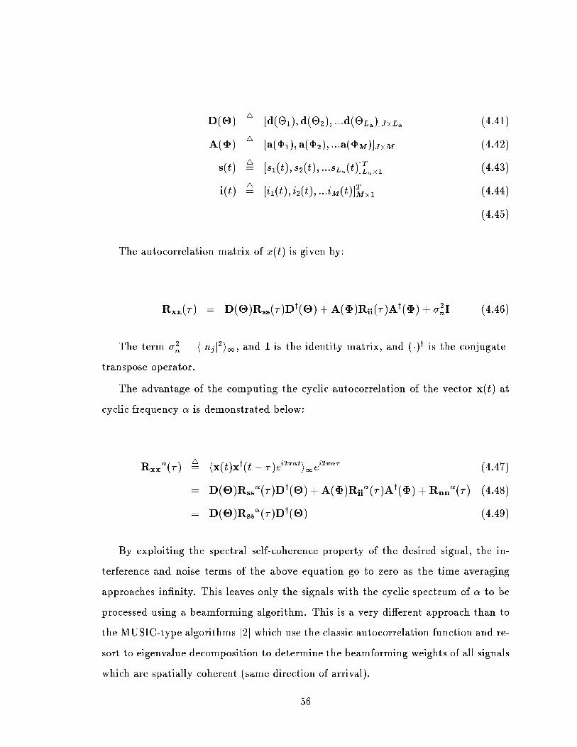
D()

4

= [d(

1

);d(

2

); :::d(

L

)]

JL

(4.41)

A()

4

= [a(

1

);a(

2

); :::a(

M

)]

JM

(4.42)

s(t)

4

= [s

1

(t); s

2

(t); :::s

L

(t)]

T

L

1

(4.43)

i(t)

4

= [i

1

(t); i

2

(t); :::i

M

(t)]

T

M1

(4.44)

(4.45)

The autocorrelation matrix of x(t) is given by:

R

xx

( ) = D()R

ss

( )D

y

() +A()R

ii

( )A

y

() +

2

n

I (4.46)

The term

2

n

= hjn

j

j

2

i

1

, and I is the identity matrix, and ()

y

is the conjugate-

transpose operator.

The advantage of the computing the cyclic autocorrelation of the vector x(t) at

cyclic frequency is demonstrated below:

R

xx

( )

4

= hx(t)x

y

(t )e

i2t

i

1

e

i2

(4.47)

= D()R

ss

( )D

y

() +A()R

ii

( )A

y

() +R

nn

( ) (4.48)

= D()R

ss

( )D

y

() (4.49)

By exploiting the spectral self-coherence property of the desired signal, the in-

terference and noise terms of the above equation go to zero as the time averaging

approaches innity. This leaves only the signals with the cyclic spectrum of to be

processed using a beamforming algorithm. This is a very dierent approach than to

the MUSIC-type algorithms [2] which use the classic autocorrelation function and re-

sort to eigenvalue decomposition to determine the beamforming weights of all signals

which are spatially coherent (same direction of arrival).

56

4.9 Blind Cyclic Spatial Filtering Algorithms

Since the theory behind cyclic time series is still relatively new, its application to this

beamforming is also quite new. There are four major techniques of beamforming to

date which employ cyclostationarity: SCORE (Spectral Coherence Restoral) [2], the

Cyclic Adaptive Beamformers [46], the Phase algorithm [34], and nally the Castedo

algorithm [34]. Recent investigation into signal subspace techniques have also been

applied to existing algorithms [5], and the motivation for this technique will be brie y

discussed below.

The performance of all these algorithms may be measured with respect to the

optimal beamforming weights. The optimal weights in terms of maximizing signal to

noise and interference (SINR) are given by [41]:

w

1;opt

= R

xx

1

d(

1

) (4.50)

Where w is the optimal beamforming weight vector.

4.9.1 Spectral Coherence Restoral Blind Beamforming Al-

gorithms (SCORE)

All SCORE algorithms aim at maximizing the spectral self-coherence of a single

frequency at the output of the beamformer using the principle of cyclostationarity.

There are a variety of cost functions which give rise to dierent algorithms with

specic advantages and applications. Least Squares SCORE and Cross SCORE are

the two techniques which are dealt in detail in this thesis.

4.9.1.1 Least-Squares SCORE

The Least-Squares SCORE is the simplest algorithm which employs spectral self-

coherence. This technique is applicable to the rank L

= 1 environment where there

is only one signal with the frequency spectrum .

57

The rst step in the LS-SCORE algorithm is to dene the reference signal:

u(t)

4

= c

y

x

()

(t )e

i2t

(4.51)

This reference signal has a component which is correlated with the desired signal

(s(t)) and a component which is uncorrelated (i(t);n(t)) The optional conjugation

operator ()

()

is employed depending on the type of spectral self-coherence to be

exploited. The value of the control vector c is a xed constant, and does not aect

the performance of the algorithm.

The beamforming weights are found by performing a least squares minimization

of the distance between the reference signal and the output signal y(t):

y(t)

4

= w

y

x(t) (4.52)

This results in the requirement:

min

whjy(t) u(t)j

2

i

N

(4.53)

Here N is the number of samples of x available to the algorithm.

The familiar optimal solution to (4.53) as N !1 is [34]:

w

opt

! R

xx

1

r

xu

(4.54)

= R

xx

1

R

xx

( )ce

j

(4.55)

(4.56)

For this application of the LS-SCORE algorithm, it is assumed that the in-

terference and the noise terms are not spectrally coherent at the frequency spec-

trum and that only one desired signal has the frequency spectrum . Therefore

R

xx

( ) = d(

1

)d

y

(

1

)R

ss

is a rank-one matrix. 4.56 reduces to:

w

opt

= [d

y

(

1

)R

ss

c e

j

]R

xx

1

d(

1

) (4.57)

= R

xx

1

d(

1

) (4.58)

58

Where is a complex-valued constant.

Therefore as N !1 the Least Squares SCORE algorithm converges to the SINR

optimal beam weight.

The main advantage of the Least Squares score is its computational simplicity. The

cost for this simplicity is a slow convergence rate. Analysis done in [34] attributes

the slow convergence rate to the weak feature strength or spectral self-coherence

generated by the algorithm, and its inability to quickly reject strong interferers.

An improvement to the Least Squares SCORE algorithm is to adaptively modify

the control vector c. This give rise to the Cross Score algorithm.

4.9.1.2 Cross SCORE Algorithm

The Cross SCORE algorithm uses the received signal y(t) and the reference signal

u(t) to adaptively update both the control vector c and the weight vector w. The

algorithm maximizes the temporal cross-correlation coecient, j

yu

( )j

2

dened anal-

ogously to equation (4.33) resulting in the following cost function:

max

w; c j

yu

( )j

2

,

max

w; c

jw

y

R

xx

( )cj

2

[w

y

R

xx

w][c

y

R

xx

c]

(4.59)

The Rayleigh Quotient cost function for w arises when w in (4.59) is xed. The

maximal value for c = R

xx

1

R

xx

y

( )w is substituted:

max

w

w

y

R

xx

1

( )R

xx

y

( )w

w

y

R

xx

w

(4.60)

By solving a standard eigenvalue problem, solutions to Equation (4.60) may found.

The solution to the Cross Score algorithm is achieved using the optimal expression for

c, and by using the pair of eigenvectors corresponding to the maximum eigenvalues

of the two equations below:

R

xx

( )R

xx

1

R

xx

y

( )w = R

xx

w (4.61)

R

xx

( )R

xx

1

R

xx

y

( )c = R

xx

c (4.62)

59

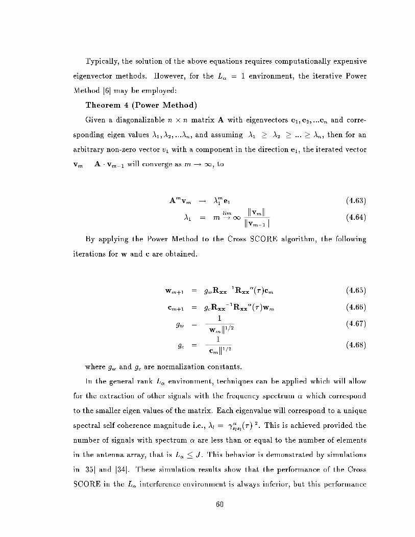
Typically, the solution of the above equations requires computationally expensive

eigenvector methods. However, for the L

= 1 environment, the iterative Power

Method [6] may be employed:

Theorem 4 (Power Method)

Given a diagonalizable n n matrix A with eigenvectors e

1

; e

2

; :::e

n

and corre-

sponding eigen values

1

;

2

; :::

n

, and assuming j

1

j j

2

j :::

n

, then for an

arbitrary non-zero vector v

1

with a component in the direction e

1

, the iterated vector

v

m

= A v

m1

will converge as m!1, to

A

m

v

m

!

m

1

e

1

(4.63)

1

=

lim

m!1

kv

m

k

kv

m1

k

(4.64)

By applying the Power Method to the Cross SCORE algorithm, the following

iterations for w and c are obtained.

w

m+1

= g

w

R

xx

1

R

xx

( )c

m

(4.65)

c

m+1

= g

c

R

xx

1

R

xx

( )w

m

(4.66)

g

w

=

1

kw

m

k

1=2

(4.67)

g

c

=

1

kc

m

k

1=2

(4.68)

where g

w

and g

c

are normalization constants.

In the general rank L

environment, techniques can be applied which will allow

for the extraction of other signals with the frequency spectrum which correspond

to the smaller eigen values of the matrix. Each eigenvalue will correspond to a unique

spectral self coherence magnitude i.e.,

l

= j

s

l

s

l

( )j

2

. This is achieved provided the

number of signals with spectrum are less than or equal to the number of elements

in the antenna array, that is L

J . This behavior is demonstrated by simulations

in [35] and [34]. These simulation results show that the performance of the Cross

SCORE in the L

interference environment is always inferior, but this performance

60

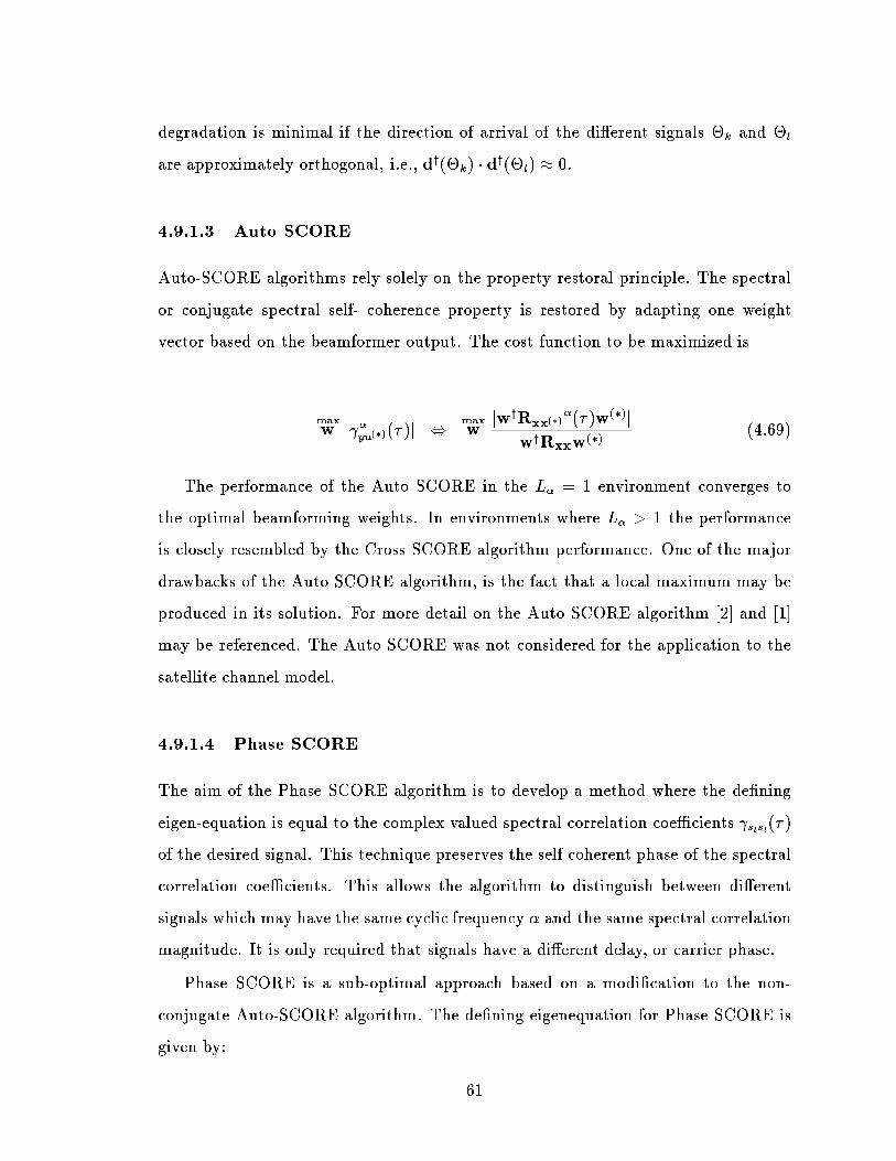
degradation is minimal if the direction of arrival of the dierent signals

k

and

l

are approximately orthogonal, i.e., d

y

(

k

) d

y

(

l

) 0.

4.9.1.3 Auto SCORE

Auto-SCORE algorithms rely solely on the property restoral principle. The spectral

or conjugate spectral self- coherence property is restored by adapting one weight

vector based on the beamformer output. The cost function to be maximized is

max

wj

yu

()

( )j ,

max

w

jw

y

R

xx

()

( )w

()

j

w

y

R

xx

w

()

(4.69)

The performance of the Auto SCORE in the L

= 1 environment converges to

the optimal beamforming weights. In environments where L

> 1 the performance

is closely resembled by the Cross SCORE algorithm performance. One of the major

drawbacks of the Auto SCORE algorithm, is the fact that a local maximum may be

produced in its solution. For more detail on the Auto SCORE algorithm [2] and [1]

may be referenced. The Auto SCORE was not considered for the application to the

satellite channel model.

4.9.1.4 Phase SCORE

The aim of the Phase SCORE algorithm is to develop a method where the dening

eigen-equation is equal to the complex valued spectral correlation coecients

s

l

s

l

( )

of the desired signal. This technique preserves the self coherent phase of the spectral

correlation coecients. This allows the algorithm to distinguish between dierent

signals which may have the same cyclic frequency and the same spectral correlation

magnitude. It is only required that signals have a dierent delay, or carrier phase.

Phase SCORE is a sub-optimal approach based on a modication to the non-

conjugate Auto-SCORE algorithm. The dening eigenequation for Phase SCORE is

given by:

61

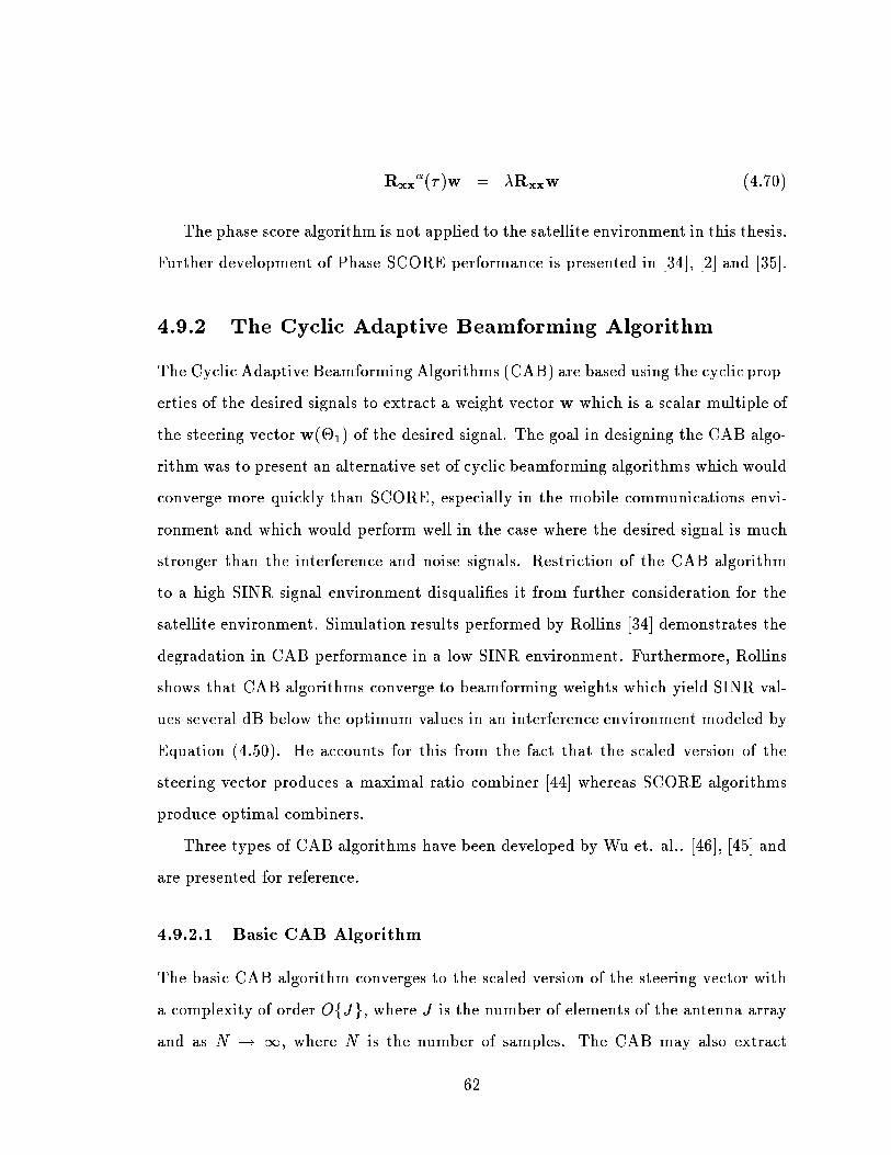
R

xx

( )w = R

xx

w (4.70)

The phase score algorithm is not applied to the satellite environment in this thesis.

Further development of Phase SCORE performance is presented in [34], [2] and [35].

4.9.2 The Cyclic Adaptive Beamforming Algorithm

The Cyclic Adaptive Beamforming Algorithms (CAB) are based using the cyclic prop-

erties of the desired signals to extract a weight vector w which is a scalar multiple of

the steering vector w(

1

) of the desired signal. The goal in designing the CAB algo-

rithm was to present an alternative set of cyclic beamforming algorithms which would

converge more quickly than SCORE, especially in the mobile communications envi-

ronment and which would perform well in the case where the desired signal is much

stronger than the interference and noise signals. Restriction of the CAB algorithm

to a high SINR signal environment disqualies it from further consideration for the

satellite environment. Simulation results performed by Rollins [34] demonstrates the

degradation in CAB performance in a low SINR environment. Furthermore, Rollins

shows that CAB algorithms converge to beamforming weights which yield SINR val-

ues several dB below the optimum values in an interference environment modeled by

Equation (4.50). He accounts for this from the fact that the scaled version of the

steering vector produces a maximal ratio combiner [44] whereas SCORE algorithms

produce optimal combiners.

Three types of CAB algorithms have been developed by Wu et. al.. [46], [45] and

are presented for reference.

4.9.2.1 Basic CAB Algorithm

The basic CAB algorithm converges to the scaled version of the steering vector with

a complexity of order OfJg, where J is the number of elements of the antenna array

and as N ! 1, where N is the number of samples. The CAB may also extract

62

multiple signals with the cyclic frequency spectra , provided the direction of arrival

of the signals are approximately orthogonal.

4.9.2.2 Constrained CAB Algorithm (C-CAB)

C-CAB exploits the property that the CAB algorithm converges to a scaled version

of the steering vector. The w

CAB

estimation of the direction of arrival of the desired

signal is used as an input to the linearly-constrained minimum variance (LCMV)

beamforming algorithm [41]. The computational complexity of this problem is of

order OfJ

2

g

4.9.2.3 Robust CAB Algorithm (R-CAB)

The R-CAB algorithm has a modied cost function that reduces the eect of small

perturbations in R

ii

and d(

l

). R-CAB requires an estimation of R

ii

which requires

the complexity of order OfJ

3

g.

4.9.3 Castedo Algorithm

This algorithm is based upon the observation that cyclostationary signals exhibit

spectral lines in the frequency domain when passed through non-linear transforms.

The algorithm attempts to minimize the mean square error of these spectral lines

with a known generated reference tone corresponding to one of the spectral lines

[7]. Spectral lines are generated by the non-linear transform ()

p

where p 2 at the

following frequencies:

y(t) =

^

E

fx

p

(t)g (4.71)

4

=

^

E

0

fx

p

(t)e

i2t

ge

i2t

(4.72)

= m

px

e

i2t

(4.73)

Cyclic beamforming weights may be calculated by using the following cost func-

tion:

63

J = hje

i2t

y

p

(t)j

2

i

1

(4.74)

Here, the beamformer output is the scalar y(t) = w

y

x(t)

The Equation (4.74) may be minimized using the method of steepest descent,

resulting in the iteration:

w(t+ 1) = w(t) r

w(t)

J (4.75)

In 4.75 represents the step-size parameter, and r

w(t)

J represents the gradient

of w. This results in the following iterative algorithm for nding the beam weights:

w(t+ 1) = w(t) +

(t)y

p1

(t)x (4.76)

Where the error signal is the term = e

i2t

y

p

(t).

The performance of the Castedo algorithm is highly dependent upon the stationary

points which are generated under dierent signal environments. A summary of the

conditions for optimal convergence are presented in [7] and [34]

4.9.4 PHASE Algorithm

A new PHASE algorithm has been proposed by Cui in [9] for application in a wireless

indoor environment. In the Phase algorithm, the output of each array element is

spectrally correlated. A reference signal u

j

(t) = x

j

(t)e

2t

is applied to the steering

vector.

r

j

4

= hx(t)u(t)i

N

(4.77)

This results in a set of cyclic correlation vectors, in which the rank L

= 1

environment converges towards a scaled replica of the steering vector d(

1

). Each

64

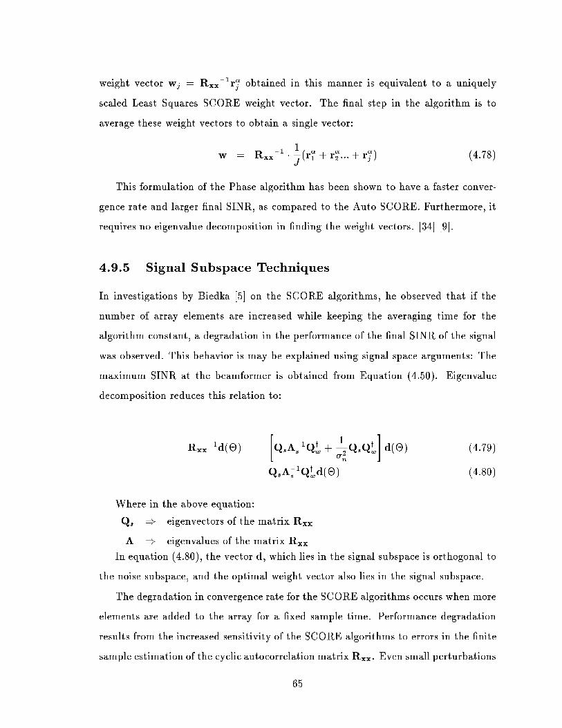
weight vector w

j

= R

xx

1

r

j

obtained in this manner is equivalent to a uniquely

scaled Least Squares SCORE weight vector. The nal step in the algorithm is to

average these weight vectors to obtain a single vector:

w = R

xx

1

1

J

(r

1

+ r

2

:::+ r

j

) (4.78)

This formulation of the Phase algorithm has been shown to have a faster conver-

gence rate and larger nal SINR, as compared to the Auto SCORE. Furthermore, it

requires no eigenvalue decomposition in nding the weight vectors. [34] [9].

4.9.5 Signal Subspace Techniques

In investigations by Biedka [5] on the SCORE algorithms, he observed that if the

number of array elements are increased while keeping the averaging time for the

algorithm constant, a degradation in the performance of the nal SINR of the signal

was observed. This behavior is may be explained using signal space arguments: The

maximum SINR at the beamformer is obtained from Equation (4.50). Eigenvalue

decomposition reduces this relation to:

R

xx

1

d() =

"

Q

s

1

s

Q

y

w

+

1

2

n

Q

s

Q

y

w

#

d() (4.79)

= Q

s

1

s

Q

y

w

d() (4.80)

Where in the above equation:

Q

s

) eigenvectors of the matrix R

xx

) eigenvalues of the matrix R

xx

In equation (4.80), the vector d, which lies in the signal subspace is orthogonal to

the noise subspace, and the optimal weight vector also lies in the signal subspace.

The degradation in convergence rate for the SCORE algorithms occurs when more

elements are added to the array for a xed sample time. Performance degradation

results from the increased sensitivity of the SCORE algorithms to errors in the nite

sample estimation of the cyclic autocorrelation matrixR

xx

. Even small perturbations

65

in the estimation of the noise matrix may cause large errors in the inverse of the cyclic

autocorrelation matrix R

xx

.

Biedka's solution to this problem is to constrain the weight vector to lie in the

signal subspace by using a low rank approximation to R

xx

[5]. Simulations by Biedka

show that the Subspace constrained SCORE algorithms exhibit signicant improve-

ments in convergence rates, compared to the standard SCORE algorithms.

The drawback to this approach is the relatively high complexity with directly

computing the eigen value decomposition of the signal space which is of order O(J

3

).

New techniques in subspace tracking may improve computational eciency. For a

brief summary of signal subspace techniques, see reference [34].

4.9.5.1 Rank-1 Power Phase SCORE Algorithm

Recent work by Rollins [34] has applied the signal sub-space method to the Phase

SCORE, and has incorporated the power method technique for arriving at the signal

weights in the rank L

=1

environment. In his study, Rollins shows that the asymptotic

values reached by Cross-SCORE and the Power Phase SCORE are the same. The

Power Phase-SCORE method is given by:

w(1; opt) = g

w

(t)

^

R

1

xx

^

R

xx

()

( )w(t) (4.81)

The matrix

^

R

1

xx

is the signal sub-space constrained estimate of the autocorrelation

of x. The major advantage of this algorithm over the Cross SCORE algorithm,

is the need to adapt only one vector, which greatly reduces the complexity of the

beamformer.

66

Chapter 5

The Modeled Channel

In this chapter, the signal model for the experimental performance evaluation will be

presented based on the statistical models, and the empirical measurements discussed

in previous chapters. The next section deals with a description of the algorithms that

will be simulated, and an account of the dierent environments that will be used to

test the robustness of the algorithms under dierent conditions.

5.1 Signal Model and Test Environment

All calculations of the signal frequencies are normalized with respect to the sampling

frequency of the system. Sampling frequencies would have to be greater than 20 MHz

based on the channel spectrum proposed in Section 3.3.

The signal processing will go through several stages. The rst stage will be the

analogue downconversion from the Ka frequency band. The desired channel will then

be frequency translated into the range of a broad band lter equal to half of the

sampling frequency. This lter will eliminate distortion due to aliasing during the

digital conversion as well as removing undesired signals from the waveform. These

steps will not be simulated in this thesis. A whitening lter may be necessary at this

stage to whiten the coloured noise generated by the broad band lter. Figure 5.1

shows the stages of the above steps. From this point on, the processing will depend

upon the proposed beamforming algorithm.

67

Analogue Anti-AliasingFilter

Analogue FrequencyTranslation

Antenna Feed To Beamformer

Analogue to DigitalConversion

Figure 5.1: Signal Processing before Beamforming

It is important to remember that the oset frequency of the carrier must not be

removed during frequency translation. This would remove the characteristic cyclic

frequency of the signal needed for the beamforming algorithms. Figure 5.2 graphically

illustrates the conversion in the frequency domain.

5.1.1 Binary Phase Shift Keying

The signal method chosen was Binary Phase Shift Keying. It was selected for a variety

of reasons, the rst of which is its simplicity for decoding. The antipodal nature of

the signal constellation also provides the greatest signal distance between dierent

symbols, which will reduce the probablily of error in a high noise environment. The

BPSK format provides cyclostationarity at self-coherent frequencies at baud rate

multiples, and at a unique conjugate self-coherence frequency at 2f

c

. Simulations

were run using the conjugate self-coherent technique [2] [34]. This will allow oset

frequencies to be assigned to dierent channels, and will allow these frequencies to be

used in the cyclostationary beamforming algorithms.

The cyclic signal strength parameter generated using conjugate self-coherent tech-

nique produces a temporal cyclic correlation coecient of unity. In contrast, cyclo-

stationary frequencies which are multiples of the baud rate produce temporal cyclic

correlation coecients of 1/6. This smaller value results in a much slower convergence

rate than for the oset carrier case [34]. Furthermore, assigning signals dierent baud

rates for identication purposes would greatly increase the complexity of the receiver

in signal recovery, and would not allow the convenience of frequency translation in

68

0Offset Channel Carrier

Ka Carrier Frequency

Message Band Guard Band

fs/20

Filter Pass Band

0 fs/2

(a)

(b)

(c)

Figure 5.2: a) Signal spectrum at the Ka Band. b) Analogue down conversion of

desired channel to the wide band anti-aliasing lter. c) Digitally sampled spectrum

of the desired channel.

69

positioning the desired channel for the anti-aliasing lter.

A detailed derivation of the calculation of the cyclic spectra of BPSK and other

modulation schemes are reported in [16].

5.1.2 Raised Cosine Pulse Shaping

The raised cosine pulse was chosen for pulse shaping [32]:

p(t) =

sin(t=T

p

)

t=T

p

cos(t=T

p

)

1 4

2

t

2

=T

2

p

(5.1)

p(t) ) pulse waveform as a function of time.

T

p

) pulse period.

) percent roll o factor.

The excess bandwidth was selected at 100 %. This value was chosen because

at the Ka frequency band, bandwidth is not a limiting factor in the system design.

The 100 % bandwidth selection makes the system more robust to sampling jitter

and intersymbol interference eects. These robustness considerations are not directly

investigated in this thesis.

In the simulations, the pulses were computed over 5 signal periods. This number

was selected as a compromise between computational speed for the simulation, as

well as in providing sucient accuracy in channel modeling.

70

5.1.3 Array Conguration

Two types of arrays were investigated. The rst array was a ve-element linear array,

with half-element spacing. This geometry was chosen for its simplicity in calculation

of the array response vector for any given direction of arrival. This basic model

allowed for easy verication of the output of the beam weights produced by the

various algorithms.

In the second array, a multiple-feed parabolic re ection antenna was calculated

using the dimensions of the antenna calculated in Section 2.2. A feed matrix was

then simulated using a parabolic array response program [11]. The target location

on the earth was selected to have a longitude of 53 degrees, and a latitude of 47.5

degrees. This corresponds to the worst case location in the coverage area as calculated

in Section 2.6.

A 5-element array was used for the purpose of beamforming on the parabolic an-

tenna. The earth coordinates of the target corresponded to 1:1 in the x-direction,

and 8:9 in the y-direction on the satellite feed plane. The method for the calcula-

tion of the feed location may be referenced in the Appendix F The geometry of the

remaining 4 points were spaced one wavelength apart in a square pattern around the

center point. The one wavelength spacing was selected to satisfy the requirements of

Section 2.3.6.

The geometry of the selected locations are presented in the Table 5.1

5.1.4 Complex Gaussian Noise Model

An additive white Gaussian noise model was used in the channel simulation. White

noise was considered the best model for the representation of the system noise which

primarily was a result of atmospheric conditions, and thermal radiation from the

earth and the satellite system. The noise vector was generated using a Gaussian

distributed envelope of various noise power levels. The phase of the generated points

were evenly distributed between 0 and 2. The noise at each antenna element was

considered independent and identically distributed.

71

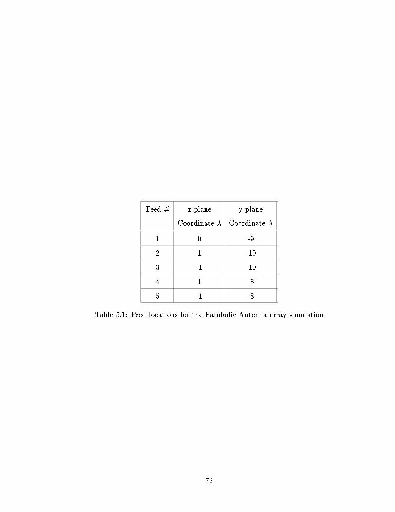
Feed # x-plane y-plane

Coordinate Coordinate

1 0 -9

2 1 -10

3 -1 -10

4 1 -8

5 -1 -8

Table 5.1: Feed locations for the Parabolic Antenna array simulation

72

Based on the calculation of the satellite link budget presented in Table 3.2, the

noise power was found to be -200.94 dBW at 20 GHz, and -201.73 dBW at 30 GHz.

This resulted in a SNR value of -51.91 dB for the 20 GHz downlink, and 64.8 dB for

the 30 GHz uplink including the parabolic antenna gain.

5.1.5 Signal Model Representation

Based on the modeling considerations presented above, the following signal model was

generated for the signal received at the antenna. This signal model was presented in

Equation (4.40) and is reproduced here for reference.

x(t) =

L

X

l=1

d(

l

)s

l

(t) +

M

X

m=1

a()i

m

+ n(t) (5.2)

= D()s(t) +A()i(t) + n(t) (5.3)

5.1.6 SINR Calculation, and Optimal Beamforming SINR

The equation for the SINR is calculated based on the above model [11]

SINR =

2

d

kw

y

d()k

2

w

y

A()R

ii

A

y

()w +

2

n

kwk

2

(5.4)

2

d

) desired signal power

2

n

) noise power

A() ) interference array matrix

d() ) desired signal direction vector

w ) beamforming weight vector

R

ii

) interference correlation matrix

To compare the performance of the beamformers, the optimal SINR of the message

signal was calculated in closed-form with the known interference direction and noise

power parameters without ltering. Using these known values, the autocorrelation

matrix R

xx

was calculated using the following steps:

73

The IID white Gaussian noise component of R

xx

was calculated resulting in the

following matrix.

2

6

6

6

6

6

6

6

6

6

6

6

6

4

2

n

0 0 ! 0

0

2

n

0 ! 0

0 0

2

n

0 0

#

0 0 ! 0

2

n

3

7

7

7

7

7

7

7

7

7

7

7

7

5

(5.5)

Next, the component of the autocorrelation of the desired signal was calculated

based on the known phase delays of the relative elements. This resulted in the complex

matrix below.

2

6

6

6

6

6

6

6

6

6

6

6

6

4

2

d

2

d

e

j2(

1

2

)

2

d

e

j2(

1

3

)

!

2

d

e

j2(

1

j

)

2

d

e

j2(

2

1

)

2

d

2

d

e

j2(

2

3

)

!

2

d

e

j2(

2

j

)

2

d

e

j2(

3

1

)

2

d

e

j2(

3

2

)

2

d

!

2

d

e

j2(

3

j

)

#

2

d

e

j2(

n

1

)

2

d

e

j2(

n

3

)

!

2

d

e

j2(

n

j1

)

2

d

3

7

7

7

7

7

7

7

7

7

7

7

7

5

(5.6)

Finally, the interference matrix was calculated in the same manner as for the

desired signal except the phase osets were scaled by the dierence in wavelength

which resulted from the dierent carrier frequency. This is indicated by the

0

notation

where is the direction of arrival of the interferer. Only one interferer was considered.

2

6

6

6

6

6

6

6

6

6

6

6

6

4

2

i

2

i

e

j2(

0

1

0

2

)

2

i

e

j2(

0

1

0

3

)

!

2

i

e

j2(

0

1

0

j

)

2

i

e

j2(

0

2

0

1

)

2

i

2

i

e

j2(

0

2

0

3

)

!

2

i

e

j2(

0

2

0

j

)

2

i

e

j2(

0

3

0

1

)

2

i

e

j2(

0

3

0

2

)

2

i

!

2

i

e

j2(

0

3

0

j

)

#

2

i

e

j2(

0

n

0

1

)

2

i

e

j2(

0

j

0

3

)

!

2

i

2

i

e

j2(

0

j

0

j

)

3

7

7

7

7

7

7

7

7

7

7

7

7

5

(5.7)

These three matrices were summed and inverted. The resulting R

xx

1

was substi-

tuted into Equation (4.50) along with the known desired signal direction to produce

74

the optimal beam forming weights.

5.2 Performance Evaluation Parameters

Several dierent test scenarios were chosen to compare the new techniques under

dierent conditions. The default environment and algorithm parameters which were

selected for the dierent test conditions are presented in Table 5.2. Table 5.3 is a list

of the variable test condition values. The test conditions are outlined below.

Total Number of Samples 2

14

Number of Samples/R

xx

2

7

Number of Symbols 3276

Number of Elements 5

# of Power Method Iterations 50

% Raised Cosine 100

# of Pulse Overlap Periods 5

Carrier Signal Magnitude 1 V

Oset Frequency of Carrier (Normalized) .25 Hz

Interference Magnitude 1

Message Signal Period (Normalized) .2 Hz

Table 5.2: Default Simulation Parameters

5.2.1 Gaussian Noise Level Test Scenario

In this test, the noise power of the environment is altered while the other test condi-

tions remain the same. The purpose of this test was to compare the performance of

dierent algorithms under dierent noise levels. This is considered the most critical

test environment.

75

Interference Frequency (f

c

10

4

), (f

c

5 10

4

)

(f

c

10

3

), (f

c

15 10

3

)

Band Pass Filter Width (Normalized) 0.4, 0.3, 0.2, 0.1, 0.05

Carrier Jitter Deviation Variance 10

8

, 2:5 10

7

, 10

6

, 2:5 10

5

Noise Vector Magnitude (Parabolic) 36.3, 40.4, 43.2, 45.3, 47.0,

48.5, 49.7, 51.7, 52.6

Noise Vector Magnitude (Linear) 0, 12.0, 18.1, 21.6, 24.1, 26.0, 27.6

Table 5.3: Variable Simulation Parameters

76

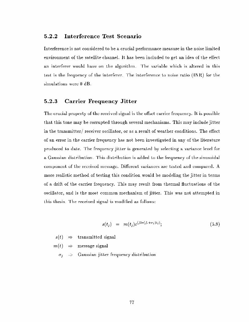
5.2.2 Interference Test Scenario

Interference is not considered to be a crucial performance measure in the noise limited

environment of the satellite channel. It has been included to get an idea of the eect

an interferer would have on the algorithm. The variable which is altered in this

test is the frequency of the interferer. The interference to noise ratio (INR) for the

simulations were 0 dB.

5.2.3 Carrier Frequency Jitter

The crucial property of the received signal is the oset carrier frequency. It is possible

that this tone may be corrupted through several mechanisms. This may include jitter

in the transmitter/ receiver oscillator, or as a result of weather conditions. The eect

of an error in the carrier frequency has not been investigated in any of the literature

produced to date. The frequency jitter is generated by selecting a variance level for

a Gaussian distribution. This distribution is added to the frequency of the sinusoidal

component of the received message. Dierent variances are tested and compared. A

more realistic method of testing this condition would be modeling the jitter in terms

of a drift of the carrier frequency. This may result from thermal uctuations of the

oscillator, and is the most common mechanism of jitter. This was not attempted in

this thesis. The received signal is modied as follows:

s(t

j

) = m(t

j

)e

(j2(f

c

+

j

)t

j

)

; (5.8)

s(t) ) transmitted signal

m(t) ) message signal

j

) Gaussian jitter frequency distribution

77

5.2.4 Oset Frequency Error Test

In this test scenario the oset frequency of the carrier is miss-matched with the

receiver cyclic frequency. In this case the desired signal is seen as an interferer.

The longer the convergence time, the greater the chance of rejection of the desired

signal by the beamforming algorithm. It is likely that the satellite and receiver

oscillators will be slightly dierent, therefore this test is seen as fairly signicant

in determining the application of the cyclic algorithms to the satellite environment.

One method proposed by [2] to minimize the eect of frequency mismatch, is to

weight the signicance of the received data points in calculating the cyclic correlation

matrix R

xx

based upon the time that the sample is received. The problem with

this technique in the satellite environment is that long correlation times are needed

to reject the high noise level, and by weighting the data, the necessary level of noise

rejection may not be possible.

5.2.5 Filter Bandwidth Test

The variable in this test scenario is the bandwidth of the front-end lter. This test

examines the eect of the distortion of the received signal which is caused by the lter

on the beamforming algorithm under dierent noise levels, and dierent lter band

widths to determine whether it is worth optimizing the bandwidth.

78

5.2.6 Simulation Test Environment Conditions

Four basic test environments were chosen to characterize the performance of the

algorithms. Single interferers were used in the interference tests. The variables in

each environment are listed below for reference:

Test Default Default Default Notes

Condition Noise Power Noise Power Bandwidth

Parabolic (dB) Linear (dB)

LNNB 40.4 12.0 .05

LNWB 40.4 12.0 .2 Filtering not tested

HNNB 47.0 21.6 .05 Filtering not tested

HNWB 47.0 21.6 .2 Noise not tested

Table 5.4: Test Environments for Beamforming Techniques

Where the above acronyms represent:

LNNB ) Low Noise Narrow Band

LNWB ) Low Noise Wide Band

HNNB ) High Noise Narrow Band

HNWB ) High Noise Wide Band

79

Chapter 6

Cyclostationary Beamforming with

Broadband Front End Filtering, and

Array Response Estimation

Two novel techniques are introduced for the purpose of beamforming in a high noise

environment. The rst of which is front end ltering the received signal before beam-

forming to reduce the magnitude of the noise power. The second technique investi-

gated uses the time lag between array elements to calculate the array response of the

system. Array response estimation is expected to reduce the time to convergence of

the algorithms.

6.1 Front End Filter Motivation

As demonstrated in Table 3.2, the Ka broadband satellite system is a noise-limited

environment. This places a dierent emphasis on beamforming algorithms than in

in the case of interference limited environments. Preliminary calculations using the

large gain of a parabolic antenna indicate that a large amount of power or gain from

the earth station (up to 74.86 dB, Table 3.2) would be required to produce a SINR

ratio suciently strong to provide a reliable link in most weather conditions. (i.e. an

outage rate of 0.01 %)

80

The literature to date has focused on cyclic beamforming environments where

the system is interference limited and the relative SINR is high, typically 0 - 20 dB.

These systems were applied to lower frequency earth based applications where there

is interference from other systems, or in multi-path environments.

Filtering was considered as a method to reduce the noise in the system. The

FRESH ltering technique employs cyclostationarity (Section 4.7) but is mainly de-

signed for eliminating interference in the system. It is also computationally expensive.

We propose basic front end digital ltering for the Ka satellite environment, in

combination with beamforming. Cyclostationarity works on the principle of rejecting

frequencies which are not equal to the cyclic frequency . The algorithm's ability to

reject other frequencies is dependent on the relative power of the desired signal and

the interference.

In Section 5.1.1 the cyclic frequency will be chosen to be twice the conjugate of

the oset frequency of the channel of interest. Since this is the only signal parameter

upon which the cyclic beamforming algorithms depend, all the other frequencies of the

received signal may be attenuated for the purpose of beamforming. This includes the

signal information as well as noise and interference. Only the carrier component must

be preserved at each antenna element. Once the beamforming weights are calculated,

they may be applied to the unltered signal, yielding the beamforming gain. A sketch

of this technique in the frequency domain is presented in Figure 6.1.

Front end ltering may be seen as a method of altering the noise subspace of

the system. From this perspective, the front end lter reduces the magnitude of the

frequency components in the noise sub-space while leaving the signal sub-space ideally

unaected.

Front end ltering avoids the need for eigenvalue decomposition or detailed knowl-

edge of the noise environment and may oer a simple method of improving cyclosta-

tionary beamforming algorithms.

81

Offset Carrier

mag

nitu

de

frequency

(a)

Offset Carrier

mag

nitu

de

frequency

(b)

Noise Magnitude

Signal Magnitude Spectrum

Filter attenuation band

Figure 6.1: a) Received waveform magnitude before ltering b) Received waveform

magnitude after ltering

82

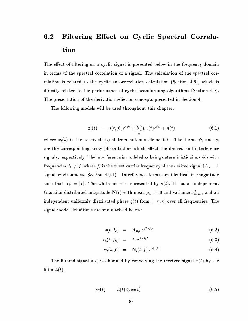
6.2 Filtering Eect on Cyclic Spectral Correla-

tion

The eect of ltering on a cyclic signal is presented below in the frequency domain

in terms of the spectral correlation of a signal. The calculation of the spectral cor-

relation is related to the cyclic autocorrelation calculation (Section 4.6), which is

directly related to the performance of cyclic beamforming algorithms (Section 4.9).

The presentation of the derivation relies on concepts presented in Section 4.

The following models will be used throughout this chapter.

x

l

(t) = s(t; f

c

)e

j

l

+

X

k

i

ljk

(t)e

j%

l

+ n(t) (6.1)

where x

l

(t) is the received signal from antenna element l. The terms

l

and %

l

are the corresponding array phase factors which eect the desired and interference

signals, respectively. The interference is modeled as being deterministic sinusoids with

frequencies f

k

6= f

c

where f

c

is the oset carrier frequency of the desired signal (L

= 1

signal environment, Section 4.9.1). Interference terms are identical in magnitude

such that jI

k

j = jIj. The white noise is represented by n(t). It has an independent

Gaussian distributed magnitude N(t) with mean

n

= 0 and variance

2

n

n

, and an

independent uniformly distributed phase (t) from [; ] over all frequencies. The

signal model denitions are summarized below:

s(t; f

c

) = jA

sig

je

j2f

c

t

(6.2)

i

k

(t; f

k

) = jIje

j2f

k

t

(6.3)

n

l

(t; f) = jN

l

(t; f)je

j

l

(t)

(6.4)

The ltered signal v(t) is obtained by convolving the received signal x(t) by the

lter h(t).

v

l

(t) = h(t) x

l

(t) (6.5)

83

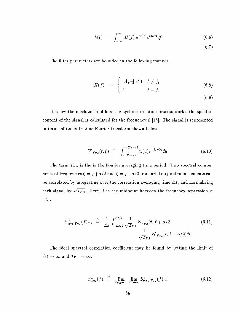
h(t) =

Z

1

1

jH(f)je

j(f)

e

j2ft

df (6.6)

(6.7)

The lter parameters are bounded in the following manner.

jH(f)j =

8

>

<

>

:

jA

filt

j < 1 f 6= f

c

1 f = f

c

(6.8)

(6.9)

To show the mechanism of how the cyclic correlation process works, the spectral

content of the signal is calculated for the frequency [15]. The signal is represented

in terms of its nite-time Fourier transform shown below:

V

ljT

FA

(t; )

4

=

Z

t+T

FA

=2

tT

FA

=2

v

l

(u)e

j2u

du (6.10)

The term T

FA

is the is the Fourier averaging time period. Two spectral compo-

nents at frequencies = f+=2 and = f=2 from arbitrary antenna elements can

be correlated by integrating over the correlation averaging time 4t, and normalizing

each signal by

p

T

FA

. Here, f is the midpoint between the frequency separation

[15].

S

v

l

v

k

jT

FA

(f)

4t

4

=

1

4t

Z

4t=2

4t=2

1

p

T

FA

V

ljT

FA

(t; f + =2) (6.11)

1

p

T

FA

V

kjT

FA

(t; f =2)dt

The ideal spectral correlation coecient may be found by letting the limit of

4t!1 and T

FA

!1.

S

v

l

v

k

(f)

4

= lim

T

FA

!1

lim

4t!1

S

v

l

v

k

jT

FA

(f)

4t

(6.12)

84

The order of the limit is important. As 4t! 1 all random terms are averaged

to their mean value. As T

FA

!1, the Fourier integral results in the rejection of all

frequencies except for f = .

If the order of the limit is changed, the limit T

FA

! 1 would decompose the

signal v

l

(t) into a discrete summation of Fourier components in the time domain or

Dirac delta functions in the frequency domain. The continuous time correlation does

not exist for discrete models when 4t <1 [16].

Figure 6.2 shows the basic processing blocks for the calculation of the cyclic cor-

relation matrix. The signal is received from the antenna, then downconverted. The

signal is time averaged to remove the random components, then is Fourier trans-

formed at the cyclic frequency. This step removes all non-random interference. The

nal processing step combines signals from other antenna elements for the calcula-

tion of the cyclic correlation matrix which is used by the beamforming algorithm to

calculate the beamweights.

The following sections will investigate how the pulse shape eects the signal model

in the calculation of the cyclic correlation matrix. A discrete time model will be used

to illustrate the eects of ltering on the signal. Limiting conditions with respect to

the lter bandwidth, and time averaging will be presented. Finally, the implications

of these ndings will be summarized.

6.2.1 Unltered Noise Sample Model

For unltered time averaging, the signal waveform is periodically sampled. The ideal

noise samples consist of uncorrelated delta functions of random Gaussian amplitude

and uniformly distributed phase in the time domain. In the frequency domain, the

signal has a constant noise power over all frequencies. The phase of the noise power

is zero. This is shown in Figure 6.3.

85

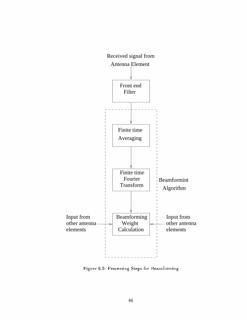
Input from other antennaelements

Input from other antennaelements

Algorithm

Beamformint

Received signal from

Front end Filter

Finite time

Averaging

Finite timeFourier

Transform

BeamformingWeight

Calculation

Antenna Element

Figure 6.2: Processing Steps for Beamforming

86

N =ο σ 2

f

f

t t

Magnitude Phase

Magnitude Phase

(a)

(b)

nn

Figure 6.3: a) Frequency Domain of the Noise Variance. b) Time Domain of Noise

Samples.

87

6.2.2 Ideal Filter Model

Equations for the ideal lter in the time and frequency domain are presented below

[19]:

jH(f)j =

8

>

<

>

:

jA

filt

j = 1 W f

c

< jf j < W + f

c

0 otherwise

(6.13)

(f) =

8

>

<

>

:

2t

o

(f) W f

c

< jf j < W + f

c

0 otherwise

(6.14)

h(t) = 2Wsinc(2W (t t

o

)) (6.15)

A diagram of the ideal lter pulse is shown in Figure 6.4.

6.2.2.1 Amplitude Distortion

The ideal lter is modeled as being uniform with zero attenuation in the passband

from W !W in the frequency domain. The Fourier transform for this pulse is the

sinc(u) = sin(u)=u pulse.

6.2.2.2 Ideal Phase

The ideal phase response of the lter consists of an angle which is a linear function

of the frequency. In the time domain this represents a time delay which is related to

the slope of the phase in the frequency domain.

6.2.2.3 Ideal Filter Impulse Response

The time domain representation of the Fourier transform of the ideal lter is shown

in Figure 6.4 (c). This sketch shows the pure time delay which results from the ideal

phase. The sinc(u) pulse is a consequence of the constant attenuation in the lter

passband.

88

t + 1/2Woto

to

fc W - fc W+

fc W+fc fc

t

Magnitude

t - 1/2Wo

2 π f

f

Phase

(b)

Magnitude

f

1

2W

(c)

(a)

W -

Figure 6.4: a) Frequency domain magnitude of an ideal lter pulse. b) Frequency

domain phase of an ideal lter pulse. c) Time domain impulse response of an ideal

lter.

89

6.2.3 Non-Ideal Filter Model

The eect of a non-ideal lter was derived to see how this changed the rate of conver-

gence of the cyclic correlation calculation. The amplitude and phase in the frequency

domain of the non-ideal lter are modeled as follows:

jH(f)j =

8

>

<

>

:

jA

filt

j = 1 W f

c

< jf j < W + f

c

0 otherwise

(6.16)

(f) =

8

>

<

>

:

2t

o

+ b sin(=Wf) W f

c

< jf j < W + f

c

0 otherwise

(6.17)

6.2.3.1 Amplitude Distortion

As mentioned in Section 6.2 the only known frequency needed for beamforming is

the cyclic frequency f

c

. This single frequency can be thought of as the message

bandwidth. Therefore as long as the cyclic frequency is not attenuated, there will be

no amplitude distortion of the carrier frequency.

As mentioned in Chapter 4 and simulated in [34], the cyclic temporal correlation

coecient depends on the magnitude of the cyclic correlation frequency . This

quantity in turn controls the convergence rate of the beamforming algorithm. A

non-uniform amplitude attenuation which meets the condition of Equation 6.8 would

have the positive eect of further attenuating the non-cyclic frequencies as compared

to the ideal lter model. The ideal lter frequency magnitude is a worst-case lter

amplitude scenario and is used for this derivation due to its simplicity in calculation.

6.2.3.2 Non-Ideal Phase

The eect of a non-ideal lter phase was investigated based on the model presented

by [19]. The phase is shown in Figure 6.5 (b). The equation of the phase as a function

of the frequency is shown in Equation 6.17. Here the constant b is assumed small

such that the rst order approximation e

j(b sin(=Wf))

= 1 + b sin(=Wf) is valid.

90

χ (f) to2 π f=

-W Wf

Phase

(b)

Magnitude

f-W W

1

(a)

+ b sin( πf/W)

Figure 6.5: a) Frequency domain magnitude of an non-ideal lter. b) Frequency

domain phase of an non-ideal lter.

91

6.2.3.3 Filter Impulse Response

The Fourier transform of the non-ideal pulse based on Equation 6.2.3.2 is derived as:

h(t) = 2Wsinc(W (t t

o

)) + (6.18)

bW [sinc(2(Wt+ 1=2)) + sinc(2(Wt 1=2))]

A time domain sketch of this pulse is shown in Figure 6.6 and 6.7. In comparison

to the ideal lter pulse, the non-ideal phase results in a wider overall signal in the

time domain.

Ideal Filter

time delayed non−ideal component

time advanced non−ideal component

−2 −1 0 1 2 3 4−0.4

−0.2

0

0.2

0.4

0.6

0.8

1

time

ampl

itude

Figure 6.6: Components of a lter with non-ideal phase response

6.2.4 Time Averaging Computation

The purpose of time averaging is to eliminate the random components of the received

signal. Equation 6.1 models the random noise signal in terms of two independent

processes, the zero Gaussian mean and the zero mean uniformly distributed phase.

These two processes are ergodic [32].

92

Non−Ideal Filter Time ResponseIdeal Filter Time Response

−2 −1 0 1 2 3 4−0.4

−0.2

0

0.2

0.4

0.6

0.8

1

time

ampl

itude

Figure 6.7: Comparison of a ideal and non-ideal lter pulse in response showing pulse

widening.

93

6.2.4.1 Independent Time Samples

For the calculation of independent time samples, the time averaged mean may be

found by [32]:

= lim

4t!1

1

N

4t

N

4t

X

i=1

x

i

(6.19)

= (6.20)

where is the sample mean and N

4t

is the number of noise samples. The rate of

convergence to the true mean is 1=N

4t

.

The unbiased sample variance of independent signals for an unknown mean can

be estimated as [32]:

2

n

l

n

l

=

1

(N

4t1)

N

4t

X

i=1

2

n

l

n

l

ji

(6.21)

6.2.4.2 Correlated Time Samples

When the time samples are correlated, the time to convergence is aected by a factor

which depends on the amount of correlation among the samples:

N

4t

;K

4

=

N

4t

X

i=0

K

X

k=K

j

c

(i k)j (6.22)

=

1

N

4t

N

4t

X

i=0

K

X

k=K

c

(i k)x

k

(6.23)

<

N

4t

;K

N

4t

N

4t

X

i=0

x

i

(6.24)

where

N

4t

;K

is the correlation coecient sum, 2K is the correlation period, and

c

(i k) is the correlation between time samples i and k.

The time averaged term will converge almost surely to the true mean in the

limit as 4t!1 if

N

4t

;K

is nite.

94

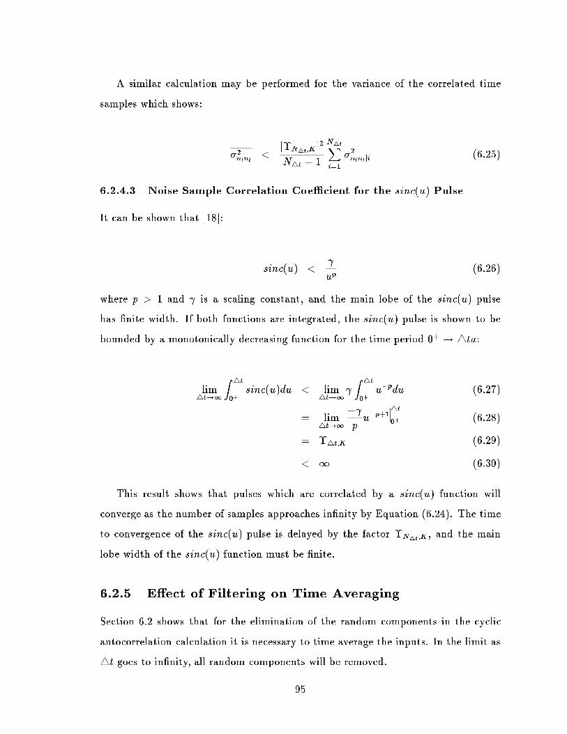
A similar calculation may be performed for the variance of the correlated time

samples which shows:

2

n

l

n

l

<

[

N

4t

;K

]

2

N

4t

1

N

4t

X

i=1

2

n

l

n

l

ji

(6.25)

6.2.4.3 Noise Sample Correlation Coecient for the sinc(u) Pulse

It can be shown that [18]:

sinc(u) <

u

p

(6.26)

where p > 1 and is a scaling constant, and the main lobe of the sinc(u) pulse

has nite width. If both functions are integrated, the sinc(u) pulse is shown to be

bounded by a monotonically decreasing function for the time period 0

+

!4ta:

lim

4t!1

Z

4t

0

+

sinc(u)du < lim

4t!1

Z

4t

0

+

u

p

du (6.27)

= lim

4t!1

p

u

p+1

4t

0

+

(6.28)

=

4t;K

(6.29)

< 1 (6.30)

This result shows that pulses which are correlated by a sinc(u) function will

converge as the number of samples approaches innity by Equation (6.24). The time

to convergence of the sinc(u) pulse is delayed by the factor

N

4t

;K

, and the main

lobe width of the sinc(u) function must be nite.

6.2.5 Eect of Filtering on Time Averaging

Section 6.2 shows that for the elimination of the random components in the cyclic

autocorrelation calculation it is necessary to time average the inputs. In the limit as

4t goes to innity, all random components will be removed.

95

The lter has the eect of spreading out the input waveform in the time domain.

Hence, the uncorrelated unltered noise becomes correlated after ltering. This re-

duces the eectiveness of time averaging and increases the required correlation time

(Section 6.2.4.3).

Furthermore, for the case where the lter's phase response is given by Equation

6.17 , the pulse is spread out more. This is shown in Figure 6.7. The larger the

deviation from the ideal phase response, the larger the pulse spread, and therefore

the longer the required averaging time to reach convergence. It is important to note

that as long as the main lobe of the sinc(u) pulse is nite in the duration, the limit

as 4t!1 is not aected.

6.2.6 Eect of Filtering on the Noise Power

The fact that the noise is limited to the frequency band from W ! W for the

ltered signal, reduces the noise power of the system. This increases the SNR of the

input signal to the beamformer which improves the convergence rate. Simulations by

[34] and [2] show that the higher the SNR value, the quicker the rate of convergence

for cyclostationary beamforming algorithms.

6.2.7 Limit as the Filter Bandwidth Approaches Innity

The eect of letting the lter bandwidth approach innity is considered:

6.2.7.1 Eect on Filter Amplitude

As the lter bandwidth W ! 1, the lter impulse response is more concentrated.

In the limit, the lter impulse response becomes a delta function. This is the case

for both the ideal and non-ideal lter model and is identical to the pulse of the

non-ltered noise sample.

96

6.2.7.2 Eect on Filter Phase

The widening of the lter bandwidth will have the eect of reducing the slope of the

lter phase in the frequency domain. This will result in a decrease in the time delay.

For the non-ideal lter case, the distortion and the corresponding time pulse dilation

will also be reduced. In the limit, the phase delay and distortion would be zero for

both the ideal and non-ideal lter.

6.2.7.3 Eect on Time Averaging

When the lter bandwidth reaches innity, the correlation of the dierent time sam-

ples is removed. Therefore there is no degradation in the time averaging performance

of the algorithms. The resulting calculation is identical to the non-ltered scenario.

6.2.7.4 Eect on Noise Power

The broadening of the lter bandwidth results in a rejection of fewer noise frequency

components. As a result the noise power increases. In the limit, the input noise power

is identical to the non-ltered condition.

6.2.8 Limit as the Filter Bandwidth Approaches Zero

In this limit, the lter bandwidth is narrowed to reject all frequencies other than the

oset carrier frequency needed for beamforming.

6.2.8.1 Eect on Filter Amplitude

As the lter's bandwidth becomes more narrow, the impulse response becomes more

dilated in the time domain for both the ideal and non-ideal signal model. When the

limit is reached, the lter signal is uniform for all time.

97

6.2.8.2 Eect on Filter Phase

The compression of the lter bandwidth will have the result of increasing the slope

of the phase for the ideal lter response. This will result in the pulse having a longer

delay.

For the non-ideal case, the phase distortion will become greater as the bandwidth

decreases. Based on Equation 6.17, this corresponds to an increase in the magnitude

of the constant b. As a result, the time domain response will be further dilated.

6.2.8.3 Eect on Time Averaging

For the ideal lter the dilation of the impulse response in the time domain will decrease

the eectiveness of time averaging, as the correlation time among samples becomes

longer. The pure phase delay will not aect the time averaging convergence rate.

In the case of the non-ideal lter, both the dilation due to the magnitude, and

the dilation due to an increase in the phase distortion will degrade the eectiveness

of time averaging on the reduction of the noise power.

When the lter frequency response reaches the limit (f f

c

) for both the ltered

and unltered cases, the impulse response will be uniform for all values of time,

and the period of the sinc(u) pulse will be innite. As a result, the random noise

component at the carrier frequency will not be removed due to time averaging.

6.2.8.4 Eect on Noise Power

When the lter frequency response reaches the limit (f f

c

), only the noise which

is present at the carrier frequency remains. As explained in Section 6.2.8.3, time

averaging will not reduce this random component.

6.2.9 Finite Time Fourier Transform

The function of the nite time Fourier transform is to reject the non-random inter-

ference signals at frequencies other than the cyclic frequency. The nite time Fourier

98

transform acts much like a brickwall lter whose passband becomes more narrow as

the averaging time increases.

With reference to Equation 6.10, the transform for the ltered signal at the cyclic

frequency after the random frequency components have been averaged to zero can

be written as:

V

ljT

FA

() = jA

sig

je

j

l

+

K

X

k=1

jIjjH(f

k

)je

j(f

k

+%

l

)

sinc(( f

k

)(T

FA

)) (6.31)

The lter's eect does not alter the cyclic carrier frequency information and does

attenuate the interference signals which would increase the rate of interference rejec-

tion [34]. The eect of the nite time Fourier transform can be compared to the case

for ideal ltering where the lter passband narrows to a point about f

c

.

It should be noted that the lter introduces a phase component to the interference

signal. This would harm the performance of beamforming techniques which introduce

beam pattern nulls to block out interferers. Since this thesis focuses on a noise-limited

channel, such an investigation was not pursued.

6.2.10 Summary of Filtering's Eects on Beamforming

The goal of ltering is to reduce the input noise power into the beamformer under

conditions where the signal environment is noise limited. The only signal criteria that

must be preserved is the cyclic carrier frequency. Based on the preceding sections,

the following statements can be made:

6.2.10.1 Noise Power Reduction

As shown in Section 6.2.6, the lter reduces the noise power input to the system.

This noise power reduction increases as the bandwidth decreases, and in this manner

increases the SNR of the signal input into the beamformer. The increase in the SNR

will improve the convergence rate of the algorithm [34] [2]. The only condition on the

lter magnitude is that the cyclic carrier frequency not be attenuated.

99

6.2.10.2 Eect of Filtering on Time Averaging

The cyclic correlation calculation is based on the principal of ergodicity. In the

unltered condition, all time samples are modeled as being statistically independent.

Therefore time averaging reduces the random signal's variance at a rate of 1=(N

4t

1)

for the condition of unknow phase [29]. Here, N

4t

corresponds to the number of noise

samples of the signal.

Filtering has the following two eects on the rate of time averaging:

Limiting the input noise frequencies results in a sinc(u) pulse shape (Section

6.2.2). The dilation of the noise samples in the time domain correlates the

samples and in turn decreases the rate of convergence. It is possible that under

low noise conditions, the correlation of the time samples will outweight the

eects of noise power rejection. Therefore, ltering is predicted to be most

benecial in noise limited environments. This will be veried in the simulation

tests.

In the case of non-ideal ltering, the phase distortion also results in a dilation

of the signal pulse (Section 6.2.3.2). The phase dilation increases as the lter

bandwidth decreases the rate of convergence (Section 6.2.3.2).

6.2.10.3 Eect of Filtering on Convergence

In Section 6.2.5 it was shown that as long as the lter impulse response was nite,

the eects of time averaging would reduce the random eects of the received signal,

and the ltered and unltered signals would be the same in the limit as 4t!1.

The rate of convergence depends on the trade-o between the lter's noise reduc-

tion (Section 6.2.6), and the input pulse's time dilation.

6.2.10.4 Motivation for Phase Compensation

An eective method of reducing the time dilation and improving the time averaged

variance reduction is through phase compensation of the ltered signal. Since the

100

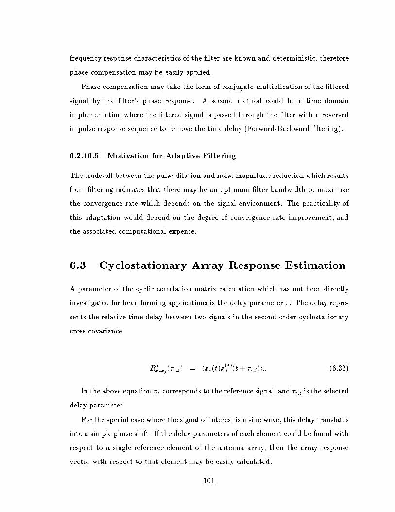
frequency response characteristics of the lter are known and deterministic, therefore

phase compensation may be easily applied.

Phase compensation may take the form of conjugate multiplication of the ltered

signal by the lter's phase response. A second method could be a time domain

implementation where the ltered signal is passed through the lter with a reversed

impulse response sequence to remove the time delay (Forward-Backward ltering).

6.2.10.5 Motivation for Adaptive Filtering

The trade-o between the pulse dilation and noise magnitude reduction which results

from ltering indicates that there may be an optimum lter bandwidth to maximize

the convergence rate which depends on the signal environment. The practicality of

this adaptation would depend on the degree of convergence rate improvement, and

the associated computational expense.

6.3 Cyclostationary Array Response Estimation

A parameter of the cyclic correlation matrix calculation which has not been directly

investigated for beamforming applications is the delay parameter . The delay repre-

sents the relative time delay between two signals in the second-order cyclostationary

cross-covariance.

R

x

r

x

j

(

r;j

) = hx

r

(t)x

()

j

(t+

r;j

)i

1

(6.32)

In the above equation x

r

corresponds to the reference signal, and

r;j

is the selected

delay parameter.

For the special case where the signal of interest is a sine wave, this delay translates

into a simple phase shift. If the delay parameters of each element could be found with

respect to a single reference element of the antenna array, then the array response

vector with respect to that element may be easily calculated.

101

It must be noted that the reference sinusoid must be one of the antenna elements

of the array, not an independently generated sinusoid. This necessity arises from the

fact that the array sinusoid is modulated according to some unknown bit sequency. If

this message modulation is not present, the signals will not converge. This behavior

was tested in simulations.

An algorithm for the estimation of the array response based on the relative delay

among elements is proposed using a simple binary search algorithm. Two delay values

corresponding to the start and end of the period of the oset sinusoid were chosen.

The cyclic correlation was calculated for the upper and lower bound of the delays

selected. A binary search algorithm was implemented. The delay resulting in the

largest calculated value of the real component of the temporal correlation coecient

was selected as the next bound in the binary search.

When the exact delay factor is found, the real part of the temporal correlation

coecient is equal to 1.

The array response estimation technique proposed can be compared to several

algorithms existing in the literature. It is most similar to the Phase estimation tech-

nique (Section 4.9.4) in that both algorithms use an antenna element as a reference

signal to estimate the array response. The Phase algorithm uses a least squares cost

function while the Array estimation technique performs a search of the time delay

value which will maximize the real part of the temporal correlation coecient.

The application of the cyclic array response estimation is to provide a method

of calculating the array response of the antenna which may be updated dynamically,

and which will be robust with respect to errors or component failures. Applications

may also be used to nding direction of arrival for simple antenna geometries.

102

6.4 Front End Filtered SCORE Beamforming Tech-

niques

Two basic beamforming algorithms were selected for application to the linear antenna

array and for the parabolic antenna array in the L

= 1 environment. The least

squares algorithm was chosen for its simplicity, and to give a lower bound on the

performance of an algorithm with minimal computational complexity. The Cross-

Score algorithm was selected based on its superior convergence rate. Many of the

algorithms presented in literature aim at reducing the computational complexity of

the Cross SCORE while maintaining the same convergence rate, or improving the

algorithms in an interference environment.

The satellite environment is modeled as a slowly time-varying. This is supported

by the condition that the earth station is stationary during transmission, and by the

observation that changing weather patterns are not fast enough to result in quickly

changing channel parameters. This allows the satellite environment the advantage

of a relatively long convergence time as compared to the mobile signal environment.

This long convergence time will be necessary in the time estimation of the cyclic

correlation matrix in a high noise environment.

The sub-space constrained techniques were not applied. The rst reason for this

is the increase in computational complexity which would result. The second reason is

that front end ltering is expected to reduce the eectiveness of the sub-space tech-

nique, though this has not been veried. Optimum implementation of the following

algorithms in terms of computation and hardware will not be investigated in detail

in this thesis. The main focus will be on the performance of the dierent algorithms

under dierent conditions.

The following sections describe the implementation of various modications of

the SCORE algorithms. Figures 6.8 and 6.9 give a graphic representation of these

schemes.

103

From Analogueto DigitalStage Beamforming

Network

From Analogueto DigitalStage

BeamformingNetwork


BeamformingNetwork

(a)

B.F.

w(t)

BeamformingAlgorithm

Message Path

(b)

H B.F.

w(t)


Message Path

Filter

(c)

H

X

B.F.

w(t)

Received Phase

Filter Magnitude


Message Path

Output to receiver

Output to receiver

Output to receiver

Figure 6.8: a) SCORE beamforming implementation b) F-SCORE beamforming im-

plementation c) PC-SCORE beamforming implementation

104

τ r,j


τ r,j


w(0)

B.F.

BeamformingNetwork

Array VectorEstimation


Message Path

H

(d)

(e)

Filter

w(0)

B.F.

BeamformingNetwork

Array VectorEstimation


Message Path

w(t) Output to receiver

w(t) Output to receiver

Figure 6.9: d)A-SCORE beamforming implementation e) FA-SCORE beamforming

implementation

105

6.4.1 SCORE Algorithm (SCORE)

The rst test condition used was the basic SCORE algorithm. (Least Squares or

Cross Score) These algorithms were applied directly to the received signal from the

antenna array. For future reference, this method will be referred to as the SCORE

implementation.

6.4.2 Filtered SCORE Algorithm (F-SCORE)

The ltered SCORE algorithm consists of a the proposed front-end lter located

along each antenna element array path. This lter's task is to remove the noise

component of the received waveform, while preserving the oset carrier signature of

the desired channel. In the simulations dierent lter bandwidths under dierent

noise environments will be examined. The basic front-end lter technique has the

advantage of being very easy to implement, with a minimal amount of computational

complexity or hardware. This technique will be referred to as F-SCORE. (Filtered

SCORE).

6.4.3 Phase Compensated SCOREAlgorithm (PC-SCORE)

In this implementation, the received signal is ltered as with the F-SCORE technique,

but the phase information received from the array is preserved or recovered. This

may be done through storing the phase data of the digitally sampled waveform before

digital ltering, and then multiplying the magnitude of the digital waveform after

ltering. Other methods would include multiplying the ltered signal by the conjugate

phase response, or by Forward-Backward ltering where the ltered signal is passed

through the lter in reverse order to remove the time delay caused by ltering. Phase

compensation ltering would be more complex and computationally expensive than

the F-SCORE described above. This beamforming method will be referred to as

PC-SCORE (Phase Compensated SCORE).

106

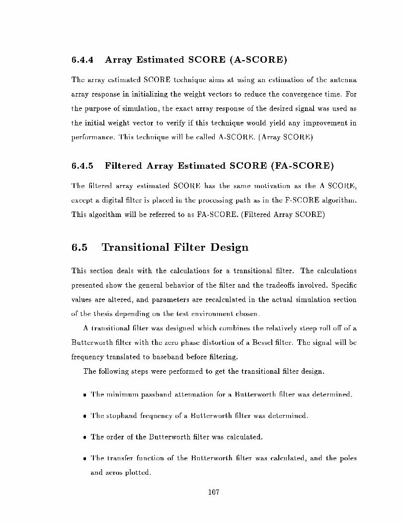
6.4.4 Array Estimated SCORE (A-SCORE)

The array estimated SCORE technique aims at using an estimation of the antenna

array response in initializing the weight vectors to reduce the convergence time. For

the purpose of simulation, the exact array response of the desired signal was used as

the initial weight vector to verify if this technique would yield any improvement in

performance. This technique will be called A-SCORE. (Array SCORE)

6.4.5 Filtered Array Estimated SCORE (FA-SCORE)

The ltered array estimated SCORE has the same motivation as the A-SCORE,

except a digital lter is placed in the processing path as in the F-SCORE algorithm.

This algorithm will be referred to as FA-SCORE. (Filtered Array SCORE)

6.5 Transitional Filter Design

This section deals with the calculations for a transitional lter. The calculations

presented show the general behavior of the lter and the tradeos involved. Specic

values are altered, and parameters are recalculated in the actual simulation section

of the thesis depending on the test environment chosen.

A transitional lter was designed which combines the relatively steep roll o of a

Butterworth lter with the zero phase distortion of a Bessel lter. The signal will be

frequency translated to baseband before ltering.

The following steps were performed to get the transitional lter design.

The minimum passband attenuation for a Butterworth lter was determined.

The stopband frequency of a Butterworth lter was determined.

The order of the Butterworth lter was calculated.

The transfer function of the Butterworth lter was calculated, and the poles

and zeros plotted.

107

A Bessel lter transfer function was calculated using the same order and stop-

band criteria as the Butterworth lter.

The S-Plane locations of the Butterworth and Bessel lter's poles and zeros

were averaged according to a chosen weighting function.

The magnitude, phase, and S-Plane coordinates were graphed for each lter.

Parameter Value

Max Passband Attenuation (dB) 3

Min Stopband Attenuation (dB) -30

Passband Frequency (MHz, Hz) 4, 1

Stopband Frequency (MHz, Hz) 5, 1.2

Filter Order 19

Butterworth Filter Weight 1

Bessel Filter Weight 3

Table 6.1: Sample Transitional Filter Data and Calculations

Normalized and scaled plots of the magnitude, phase and S-Plane poles and zeros

are plotted using the above design parameters.

The S-plane pole locations are shown in gure 6.10.

The Transitional lter shows a more gradual roll o in the transition band as

compared to the Butterworth lter as shown in gure 6.11. However its attenuation

characteristics are better than those of the Bessel lter. By adjusting the lter weights

the transitional lter may be modied to resemble the Bessel or Butterworth lter to

varying degrees.

The phase response of the transitional lter is plotted in gure 6.12. This plot

shows that the phase response of the transitional lter closely follows that of the

Bessel lter up to a normalized frequency of 0.8. The dierence between the two

plots becomes larger at the edge of the passband. Otherwise the phase distortion is

below 5:0

.

108

−1 −0.9 −0.8 −0.7 −0.6 −0.5 −0.4 −0.3 −0.2 −0.1 0−1

−0.8

−0.6

−0.4

−0.2

0

0.2

0.4

0.6

0.8

1S−plane Poles (Normal)

Butterworth

Transitional

Bessel

Figure 6.10: Plot of S plane Poles and Zeros for Butterworth, Bessel, Transitional

Filters

0 0.2 0.4 0.6 0.8 1 1.2 1.4 1.6 1.8−100

−80

−60

−40

−20

0

20Normal Mag: Butterworth, Transitional, Bessel

Butterworth

Transitional

Bessel

Figure 6.11: Plot of the Normalized Magnitude for Butterworth, Bessel, Transitional

Filters

109

0 0.2 0.4 0.6 0.8 1 1.2 1.4 1.6 1.8−200

−150

−100

−50

0

50

100

150

200Normal Phase: Butterworth, Transitional, Bessel

Butterworth

Transitional

Bessel

Figure 6.12: Plot of the Normalized Phase for Butterworth, Bessel, Transitional Fil-

ters

110

The above presented parameters produced a good realizable lter which oered

adequate attenuation while preserving the phase relation of the signal. Further in-

vestigation of the tradeo between phase and attenuation may result in lters better

designed for specic noise and interference environments (Section ??).

111

Chapter 7

SCORE Algorithm Simulation Results

7.1 Introduction

In this chapter the various test conditions are simulated for the dierent ltering

algorithms. Plots of the convergence rates of each condition are made to compare the

dierent beamforming methods. The convergence plots were done over 40 indepen-

dent iterations. The number of iterations for the power method of the Cross SCORE

was set to 50. Selected beam patterns are also plotted.

A plot of the convergence weights after 3000 symbols versus the noise level or lter

bandwidth is made for selected conditions. The lower bound on these graphs is the

SINR of a single element. For the parabolic antenna, the element with the strongest

received signal strength based on the direction of arrival was chosen.

The single element performance of the parabolic system is highly dependent on

the antenna geometry, the feed coordinates and the direction of arrival. Optimizing

these parameters was not within the scope of this thesis.

112

7.2 Cyclostationary Array Estimation Performance

of the Linear and Parabolic Antenna Cong-

uration

The cyclostationary array estimation algorithm was applied for the linear array and

the parabolic antenna. The linear array is not considered to have enough gain to

make it applicable to the high noise satellite environment, but it does oer a familiar

reference to which the algorithms' performance can be gauged.

The parabolic antenna is the antenna conguration which is most applicable to

the satellite environment based on the large gain which results from the re ector.

The linear array showed a rapid convergence under low noise conditions. This

indicates that the algorithm will work in a favourable environment.

Array

F−Array

PC−Array

0 500 1000 1500 2000 2500 3000 3500−15

−14

−13

−12

−11

−10

−9

−8

−7

−6

−5

Symbol Perods

SIN

R (

dB)

Figure 7.1: Cyclic Array Estimation Linear Array SINR Test LNNB: Received

SINR=-12 dB. *-: Optimum SINR, x-:Single Element SINR.

The convergence rate of the elements to the optimal phase was plotted for elements

113

# 1 and # 5. Figures 7.2 and 7.3 show slow convergence to the desired phase under

a low noise environment.

Array

F−Array

PC−Array

0 500 1000 1500 2000 2500 3000 3500−100

−50

0

50

100

150

200

Number of Symbols

Wei

ght A

ngle

(de

g)

Element Number 1

Figure 7.2: Cyclic Array Estimation: Element # 1 Phase Convergence Test LNNB:

Received SINR=-12 dB. *-: Optimum Angle

The performance of the parabolic antenna array is very poor even under low noise

conditions. All algorithms tend to converge very close to the SINR level of the single

strongest element. This can be seen in Figure 7.4.

Convergence performance of the algorithms to the ideal phase shows very poor

behavior. This can be seen in Figures 7.5 and 7.6. The fact that the weight angle

uctuates indicates that the calculation of the cyclic autocorrelation value of the

reference element with the selected array element is poor. The nal beam weight after

3000 symbol periods has a very large error which will greatly limit the performance

of the beamformer.

One explanation for the poor behavior of the parabolic antenna is based on the

fact that the antenna elements all have dierent received power depending on their

position on the feed plane and the direction of the incoming signal. This is very

114

Array

F−Array

PC−Array

0 500 1000 1500 2000 2500 3000 3500−170

−160

−150

−140

−130

−120

−110

−100

−90

−80

−70

Number of Symbols

Wei

ght A

ngle

(de

g)

Element Number 5

Figure 7.3: Cyclic Array Estimation: Element # 5 Phase Convergence Test LNNB:

Received SINR=-12 dB. *-: Optimum Angle

Array

F−Array

PC−Array

14 16 18 20 22 24 26 28 30 32 34 36 38 40−10

−5

0

5

10

15

Noise Magnitude (dB)

SIN

R C

alcu

latio

n

Figure 7.4: Cyclic Array Estimation Linear Array SINR Test HNNB: Received

SINR=-36 dB. *-: Optimum SINR, x-:Single Element SINR.

115

Array

F−Array

PC−Array

0 500 1000 1500 2000 2500 3000 3500−10.5

−10

−9.5

−9

Number of Symbols

Wei

ght A

ngle

(de

g)

Element Number 1

Figure 7.5: Cyclic Array Estimation Parabolic Antenna: Element # 1 Phase Conver-

gence Test HNWB: Received SINR=-36 dB. *-: Optimum Angle

116

Array

F−Array

PC−Array

0 500 1000 1500 2000 2500 3000 3500130

131

132

133

134

135

136

137

Number of Symbols

Wei

ght A

ngle

(de

g)

Element Number 5

Figure 7.6: Cyclic Array Estimation Parabolic Antenna: Element # 5 Convergence

Test HNWB Received SINR=-14 dB. *-: Optimum Angle

117

dierent compared to the linear array where all elements have approximately the same

received signal strength. As a result of this variation in the received signal among

elements, the selection of the reference element is very important in determining the

convergence rate of the algorithm for the parabolic antenna. For the test conditions

presented in this section, the relative gain of each antenna element can be referenced

in Table 7.1. This table shows that if element 5 is selected, the signal gain on the

element due to the parabolic signal would only be 12 dB. If element 3 is selected, the

re ector gain would be 30.8 dB.

Another factor which signicantly eects the convergence, is the fact that the

element with the largest signal component will converge to the correct beam weight

before the others. This may explain why the achieved SINR for the parabolic antenna

is only slightly better than the SINR of the strongest single element.

The nal factor which may contribute to the poor performance of the parabolic

antenna array is the sensitivity of the elements with a large gain to error. A slightly

incorrect temporal delay estimation could result in a large error when the power of

the elements are added after beamforming. This would result in a degradation in

performance.

These explanations are presented as hypotheses, and were not investigated further

in this thesis.

Due to the poor performance of the cyclic array estimation technique, it was

disqualied as a method for generating the array response in the high noise satellite

environment. The implementation if this array estimation technique may have an

application for linear arrays in a lower noise environment.

7.3 Eect of Array Initialization

For the conventional algorithms, the weights used for beamforming are set to an

initial value which is not related in any way to the direction of arrival of the incoming

signal. The eect of initializing the weight vector to an approximation of the direction

118

of arrival was hoped to reduce the convergence time of the SCORE algorithms. For

the algorithms considered, the initial beam weights were those which would produce

the optimal SNR.

As shown in Figure 7.28 this improvement in convergence was not observed. The

performance of SCORE, A-SCORE, and F-SCORE, FA-SCORE respectively were al-

most identical. This behavior was observed for both Least Squares and Cross SCORE

techniques, antenna congurations and all test conditions considered.

The reason for this result may be understood by referencing Equation (4.56) for

the Least Squares SCORE and (4.65) and (4.66) for the Cross SCORE algorithm.

The most important calculated value for determining the beam weights is the time

averaged estimation of the autocorrelation matrix and the cyclic autocorrelation ma-

trix. If estimation of these two values is poor, then any advantage gained by the

initialization of the beam weights is lost.

For the implementation of the Cross SCORE algorithm in the L

= 1 environment,

initialization of the weight vector should reduce the number of iterations necessary for

the convergence of the power method implementation. This computational reduction

was not expected to be signicant as compared to the time average calculation of the

cyclic correlation matrix.

It must be noted that cyclic array estimation weights were not applied to the

received data at the antenna elements but as a part of the beamforming calculation.

It is conceivable that using the cyclic array estimation directly on the received data

could improve the beamforming convergence.

7.4 Performance Comparison between Cross SCORE

and Least Squares SCORE

The two extremes of the SCORE family of algorithms were tested. The least squares

SCORE is the least complex method using the SCORE technique, while the Cross

119

SCORE

F−SCORE

PC−SCORE

A−SCORE

FA−SCORE

0 500 1000 1500 2000 2500 3000 3500−22

−21

−20

−19

−18

−17

−16

−15

−14

−13

−12

Symbol Perods

SIN

R (

dB)

Figure 7.7: Performance Comparison of Array Initialization for SCORE Algorithms.

*-: Optimum SNR, x-: Single Element SNR

120

SCORE technique is computationally the most expensive, and also has the best per-

formance.

The graphs presented in this section show the relative performance of the two

algorithms under a high noise environment for both the linear and parabolic congu-

ration. The noise performance of the algorithm was considered the most crucial test in

evaluating the suitability of an algorithm for the beamforming satellite environment

presented in this thesis.

Linear Array

The test environment considered was test LNNB which consisted of a narrow

lter bandwidth. The simulation results for the convergence rates of the least squares

SCORE and Cross SCORE are presented in Figures 7.8 and 7.9 respectively.

The least squares score shows a poor convergence rate for all techniques considered

as compared to the Cross SCORE technique when the SNR is low (-12 dB). As the

SNR decreases, beamforming performance deteriorates further. This can be noticed

by comparing the converged SINR values for the Least Squares and Cross SCORE

algorithms after 3000 symbol periods. (Figures 7.10 and 7.11)

Parabolic Antenna

The Least Squares SCORE algorithm has only a slightly worse performance as

compared the the Cross SCORE technique for low noise environments using the

parabolic antenna array. This indicates that the Least Squares SCORE algorithm

performance trade o with respect to the computational complexity may be justied

for low noise environments using a parabolic antenna (Figures 7.12 and 7.18).

The noise performance of the Least Squares SCORE algorithm quickly deteriorates

as the noise level increases as compared to the Cross SCORE algorithm. This shows

the sensitivity of the Least Squares SCORE algorithm, and its lack of robustness.

This can be seen in the Figures 7.14 and 7.15

121

SCORE

F−SCORE

PC−SCORE

0 500 1000 1500 2000 2500 3000 3500−16

−14

−12

−10

−8

−6

−4

Symbol Perods

SIN

R (

dB)

Figure 7.8: LS-SCORE Linear Array SINR, Test LNNB. Received SNR=-12 dB. *-:

Optimum SINR, x-:Single Element SINR.

122

SCORE

F−SCORE

PC−SCORE

0 500 1000 1500 2000 2500 3000 3500−15

−14

−13

−12

−11

−10

−9

−8

−7

−6

−5

Symbol Perods

SIN

R (

dB)

Figure 7.9: Cross-SCORE Linear Array SINR, Test LNNB. Received SNR=-12 dB.

*-: Optimum SINR, x-:Single Element SINR.

SCORE

F−SCORE

PC−SCORE

0 5 10 15 20 25

−25

−20

−15

−10

−5

0

5


SIN

R C

alcu

latio

n

Figure 7.10: LS-SCORE Converged SINR Linear Array Noise Performance: Test

LNNB. *-: Optimum SINR, x-:Single Element SINR

123

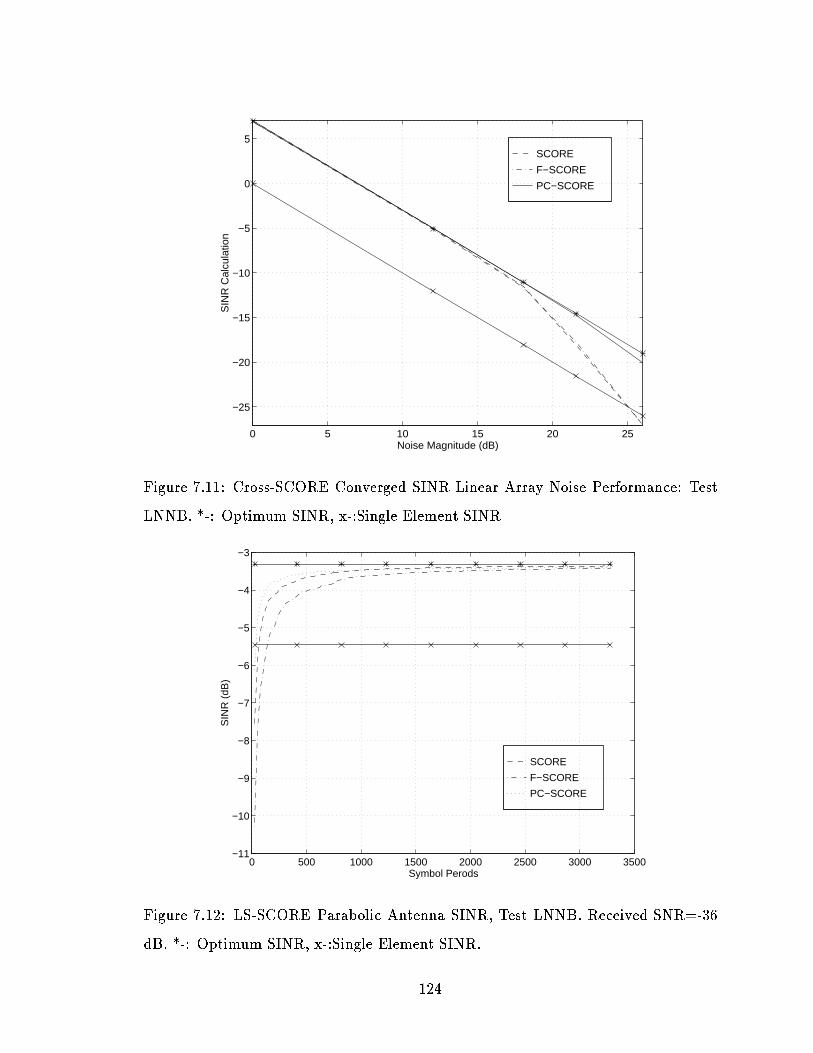
SCORE

F−SCORE

PC−SCORE

0 5 10 15 20 25

−25

−20

−15

−10

−5

0

5


SIN

R C

alcu

latio

n

Figure 7.11: Cross-SCORE Converged SINR Linear Array Noise Performance: Test

LNNB. *-: Optimum SINR, x-:Single Element SINR

SCORE

F−SCORE

PC−SCORE

0 500 1000 1500 2000 2500 3000 3500−11

−10

−9

−8

−7

−6

−5

−4

−3

Symbol Perods

SIN

R (

dB)

Figure 7.12: LS-SCORE Parabolic Antenna SINR, Test LNNB. Received SNR=-36

dB. *-: Optimum SINR, x-:Single Element SINR.

124

SCORE

F−SCORE

PC−SCORE

0 500 1000 1500 2000 2500 3000 3500−10

−9

−8

−7

−6

−5

−4

−3

Symbol Perods

SIN

R (

dB)

Figure 7.13: Cross-SCORE Parabolic Antenna SINR, Test LNNB. Received SNR=-36

dB. *-: Optimum SINR, x-:Single Element SINR.

SCORE

F−SCORE

PC−SCORE

38 40 42 44 46 48 50 52

−25

−20

−15

−10

−5


SIN

R C

alcu

latio

n

Figure 7.14: LS-SCORE Converged SINR Parabolic Antenna Noise Performance:

Test LNNB. *-: Optimum SINR, x-:Single Element SINR

125

SCORE

F−SCORE

PC−SCORE

38 40 42 44 46 48 50 52

−25

−20

−15

−10

−5


SIN

R C

alcu

latio

n

Figure 7.15: Cross-SCORE Converged SINR Parabolic Antenna Noise Performance:

Test LNNB. *-: Optimum SINR, x-:Single Element SINR

126

7.4.1 Summary of Filtered Least Square and Cross SCORE

algorithm Comparison

In all test environments considered the Cross SCORE outperforms the Least Squares

SCORE algorithm. For this reason, the Cross SCORE was considered the best can-

didate for the satellite channel used in this thesis.

The cause of this improved performance comes from the adaptation of the control

vector as well as the desired beam weight vector. This advantage is discussed in detail

in Section 4.9.1.2.

Least Squares SCORE results will not be presented in subsequent sections of this

thesis.

7.5 Comparison of the Parabolic and Linear Ar-

rays

The two antenna congurations chosen for this thesis are the parabolic and the linear

antenna. The linear antenna was selected as a simple implementation which could

oer a familiar geometry. It is easy to build, and calculations are easy to verify.

The parabolic antenna was chosen to supply the link budget with the extra gain

necessary to make the Ka band geostationary link feasible. It is the antenna design

which will be presented in the remaining sections of this thesis.

The linear array was shown to have the same performance patterns as the parabolic

antenna except at a much lower noise power level. This fact shows that the beamform-

ing algorithms tested do not depend on the array geometry. Algorithms only depend

on maximizing the characteristic cyclostationary frequency. Thus, cyclostationary

algorithms may be developed for specic environments, and could be implemented

on dierent antenna congurations without modication.

Comparison of the parabolic and linear array performance may be made using

gures presented in Section 7.4.

127

7.6 Beam Pattern Performance

The beam patterns of the various antennas, test conditions and algorithms were

plotted. These plots were used to verify if the beamforming algorithms produced a

radiation pattern which corresponds to the direction of arrival of the desired signal.

Plots are made after a correlation time of 3000 symbols.

SCORE

F−SCORE

PC−SCORE

2 2.5 3 3.5 4 4.5 5 5.55

10

15

20

25

30

35

40

45

50

Scan Angle (deg)

Gai

n dB

Figure 7.16: CS-SCORE Parabolic Antenna Beam Pattern, Test LNNB. Received

SNR=-36 dB. *-: Optimum SINR.

Figures 7.16 and 7.17 show the degradation in performance of the beam pattern

as the noise level increases. The '*-' curve shows the beam pattern based on optimum

weights. The degradation was observed to correspond to the convergence performance

for all test conditions and parameters. Only the eect of the reduction in gain due

to imperfect beamforming was investigated in this thesis. Eects such as increased

sidelobe levels and other non-idealities are an area of future investigation.

128

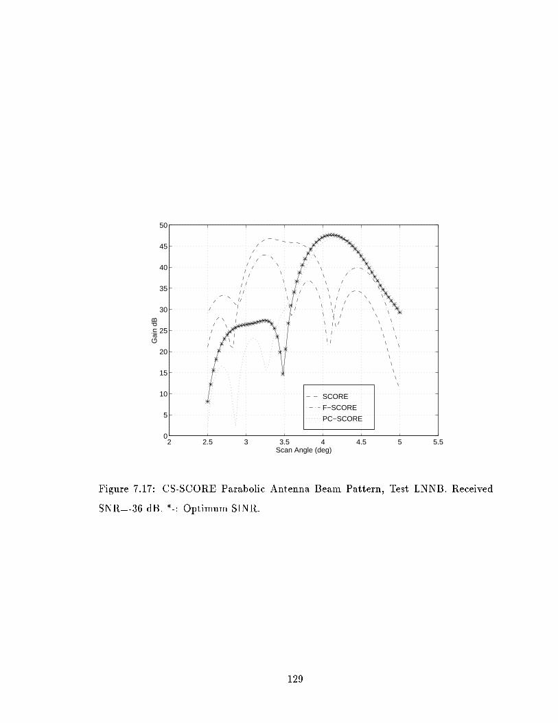
SCORE

F−SCORE

PC−SCORE

2 2.5 3 3.5 4 4.5 5 5.50

5

10

15

20

25

30

35

40

45

50

Scan Angle (deg)

Gai

n dB

Figure 7.17: CS-SCORE Parabolic Antenna Beam Pattern, Test LNNB. Received

SNR=-36 dB. *-: Optimum SINR.

129

7.7 SCORE Algorithm Convergence Performance

In the following pages, the convergence performance of the Cross SCORE parabolic

antenna array is presented. This combination of antenna geometry and beam pattern

calculation is considered most suitable to the satellite environment.

The performance of the Least Squares and linear array convergence combinations

showed the same trends as for the Cross SCORE parabolic antenna combination,

except at lower noise power levels. The explanation of the observations in the Cross

SCORE parabolic antenna environment can be applied to the Least Squares, linear

array techniques.

7.7.1 Eect of Filter Bandwidth on Convergence Perfor-

mance

The lter bandwidth is aimed at reducing the noise power which is input into the

beamformer. Section 6.2.10 describes the tradeo between noise attenuation and

pulse dilation in the time domain which aects the rate of convergence.

Performance comparisons in Figures 7.18 and 7.27 show that the SCORE algo-

rithm outperforms the F-SCORE algorithm when the lter bandwidth is narrow. If

the lter bandwidth is widened, the performance of the F-SCORE algorithm improves,

and approaches the performance of the PC-SCORE algorithm. This improvement is

more clearly seen in Figures 7.20 and 7.28 under higher noise conditions.

The degradation of F-SCORE for narrow bandwidth lters can be explained by

the increase in the pulse dilation of the ltered noise which results from the non-ideal

lter. This eect is shown in Section 6.2.3.2.

When the lter bandwidth becomes very large, the performance of all ltered

algorithms approaches the performance of the unltered SCORE method as expected

and shown in Section 6.2.7. This can be seen in Figure 7.22.

Figures 7.23 and 7.24 show the performance of the parabolic antenna of the dier-

ent algorithms for dierent lter bandwidths after a convergence time of 3000 symbols.

130

SCORE

F−SCORE

PC−SCORE

0 500 1000 1500 2000 2500 3000 3500−10

−9

−8

−7

−6

−5

−4

−3

Symbol Perods

SIN

R (

dB)

Figure 7.18: Cross SCORE Parabolic Array SINR, Test LNNB: Received SNR=-36

dB. Filter BW= .05Hz. *-: Optimum SINR, x-: Single Element SINR

131

SCORE

F−SCORE

PC−SCORE

0 500 1000 1500 2000 2500 3000 3500−7.5

−7

−6.5

−6

−5.5

−5

−4.5

−4

−3.5

−3

Symbol Perods

SIN

R (

dB)

Figure 7.19: Cross SCORE Parabolic Array SINR, Test LNWB: Received SNR=-36

dB. Filter Bandwidth= .2 Hz *-: Optimum SINR, x-: Single Element SINR

132

SCORE

F−SCORE

PC−SCORE

0 500 1000 1500 2000 2500 3000 3500−22

−20

−18

−16

−14

−12

−10

Symbol Perods

SIN

R (

dB)

Figure 7.20: Cross SCORE Parabolic Array SINR, Test LNNB: Received SNR=-42


SCORE

F−SCORE

PC−SCORE

0 500 1000 1500 2000 2500 3000 3500−22

−20

−18

−16

−14

−12

−10

Symbol Perods

SIN

R (

dB)

Figure 7.21: Cross SCORE Parabolic Array SINR, Test LNWB: Received SNR=-42


133

SCORE

F−SCORE

PC−SCORE

0 500 1000 1500 2000 2500 3000 3500−16

−15

−14

−13

−12

−11

−10

−9

−8

−7

Symbol Periods

SIN

R (

dB)

Figure 7.22: Cross SCORE Parabolic Antenna SINR, Test LNNB: Received SNR=-

40.4 dB. Filter Bandwidth= .4 Hz *-: Optimum SINR, x-: Single Element SINR

134

The relative behavior of the PC-SCORE and F-SCORE are almost identical in the

two test cases, though ltering is seen to make a signicant dierence in convergence

performance for the high noise test condition.

SCORE

F−SCORE

PC−SCORE

0.1 0.2 0.3 0.4−7.7

−7.65

−7.6

−7.55

−7.5

−7.45

Filter Bandwidth (Hz)

SIN

R C

alcu

latio

n

Figure 7.23: Cross SCORE Steady-State for SINR Parabolic Antenna, Test LNNB:

Received SNR=-40.4 dB. *-: Optimum SINR, x-: Single Element SINR

When the converged SINR is plotted versus the lter bandwidth for the linear

array after 3000 symbols, the performance dependence of the algorithms is more

dramatic. The linear array shows that there is an optimal lter bandwidth which

corresponds to a particular environment. For example, the optimal performance

bandwidth for the F-SCORE algorithm when the received SNR level is -22 dB is close

to 0.1 Hz (Test HNNB). When the received SNR is raised to -12 dB (Test LNNB),

the optimal lter bandwidth is approximately 0.2 Hz. This behavior is presented in

Figures 7.25 and 7.26. Again ltering has a signicant eect on convergence rate

performance for the linear array in a high noise environment. These trends support

the theoretical predictions presented in Section 6.2.

The variation of the lter bandwidth does not result in a signicant performance

improvement over a large range of lter values. This can be noted in Figure 7.23

where the performance gain for F-SCORE varied by only .02 dB for a lter range of

135

SCORE

F−SCORE

PC−SCORE

0.1 0.2 0.3 0.4−18.5

−18

−17.5

−17

−16.5

−16

−15.5

−15

−14.5

−14

−13.5


SIN

R C

alcu

latio

n

Figure 7.24: Cross SCORE Steady State for SINR Parabolic Antenna, Test HNNB:

Received SNR=-47 dB. *-: Optimum SINR, x-: Single Element SINR

136

1.5 Hz to 3.5 Hz.

The PC-SCORE algorithm is almost at for a bandwidth less than .3 Hz. The

signicance of this result shows that bandwidth optimization does not result in signif-

icant performance gains, and may not justify the necessary computational expense.

SCORE

F−SCORE

PC−SCORE

0.05 0.1 0.15 0.2 0.25 0.3 0.35 0.4−5.15

−5.1

−5.05

−5


SIN

R C

alcu

latio

n

Figure 7.25: Cross SCORE Steady-State for SINR Linear Array, Test LNNB:Received

SNR=-12 dB. *-: Optimum SINR, x-: Single Element SINR

7.8 Eect of Noise on Convergence Performance

The most signicant environment parameter in the evaluation of the beamforming

algorithms is the noise performance since the satellite system will be noise limited.

This section displays the convergence of the dierent algorithms with the intention of

characterizing the noise performance limit of the algorithms relative to the optimum

SNR possible. Beamforming gains which result from these simulations may be too low

for a practical system. System level changes to increase the gain would be necessary.

137

SCORE

F−SCORE

PC−SCORE

0.05 0.1 0.15 0.2 0.25 0.3 0.35 0.4−22

−21

−20

−19

−18

−17

−16

−15

−14


SIN

R C

alcu

latio

n

Figure 7.26: Cross SCORE Steady State for SINR Linear Array, Test HNNB: Re-

ceived SNR=-22 dB. *-: Optimum SINR, x-: Single Element SINR

138

7.8.1 Convergence Rate Deterioration due to Noise

Figures 7.27 to 7.29 show the degradation in the convergence rate of the Parabolic

antenna Cross SCORE method as the noise power increases. Noise performances

were not considered above 52.5 dB where the output SINR levels of all the algorithms

deteriorated below the already unsatisfactory SINR level generated by the single

element conguration. All plots show that the PC-SCORE algorithm signicantly

outperforms all other algorithms for the test cases considered.

7.8.2 SCORE Convergence Limit due to High Noise

In Figure 7.29 the SCORE and F-SCORE show no indication of convergence after

3000 symbol periods. For the basic SCORE algorithm the poor noise performance

may be explained by the need for a longer convergence time to reject the noise. For

the F-SCORE algorithm the pulse dilation due to ltering may result in the poor

performance. These eects are explained in Section 6.2.

The PC-SCORE technique shows a signicant convergence rate performance im-

provement over F-SCORE. This supports the argument that the calculation of the

SCORE beamforming algorithms have a critical dependence on the phase of the in-

coming signal data (Section 6.2.3).

The performance of the SINR convergence after 3000 symbols with respect to the

noise power level is presented in Figure 7.30. This gure indicates that there is a

threshold level at which the performance of the algorithms begin to deteriorate.

7.8.3 Cross SCORE Noise Performance Summary

The cross SCORE parabolic antenna conguration modeled in this thesis can provide

an antenna gain of 31 dB. An optimum beamforming gain of 2 dB could be achieved

at a received SNR level as low as -45 dB and -48 dB for F-SCORE and PC-SCORE

respectively. This resulted in SNR levels of less than -10 dB which are too low for a

reliable communications system. Therefore, a practical system would have to provide

139

SCORE

F−SCORE

PC−SCORE

0 500 1000 1500 2000 2500 3000 3500−7.5

−7

−6.5

−6

−5.5

−5

−4.5

−4

−3.5

−3

Symbol Perods

SIN

R (

dB)

Figure 7.27: Cross-SCORE Parabolic Array SINR, Test LNWB. Received SNR=-36

dB. *-: Optimum SINR, x-: Single Element SINR

140

SCORE

F−SCORE

PC−SCORE

0 500 1000 1500 2000 2500 3000 3500−22

−20

−18

−16

−14

−12

−10

Symbol Perods

SIN

R (

dB)



141

SCORE

F−SCORE

PC−SCORE

0 500 1000 1500 2000 2500 3000 3500−30

−28

−26

−24

−22

−20

−18

−16

Symbol Perods

SIN

R (

dB)



SCORE

F−SCORE

PC−SCORE

38 40 42 44 46 48 50 52

−25

−20

−15

−10

−5


SIN

R C

alcu

latio

n

Figure 7.30: Cross-SCORE Steady State SINR Parabolic Antenna Noise Performance:

Test LNWB. *-: Optimum SINR, x-: Single Element SINR

142

an additional 15 to 25 dB of gain. This may be obtained using higher gain antennas,

or through increasing the beamforming gain by using more antenna elements.

The relatively long correlation time of 3000 symbols is possible because of the

slowly time varying nature of the system modes (Section 3.2). This long convergence

time is not possible with quickly changing environments such as in the case of mobile

users, or interference limited channels.

7.9 Eect of Interference on Convergence Perfor-

mance

The eect of interference on convergence is not expected to be signicant for the test

environments considered due to the fact that the interference power is much less than

the noise power level. Simulations were run to verify this statement. The interferer

was modeled as being in the same direction as the desired signal with the same power

level. The only dierence is the oset frequency.

Figures 7.31 and 7.32 show that even under narrow ltering and relatively low

noise environment of test condition LNNB, there is no signicant eect of introducing

the interference signal on the convergence rate.

The reason for this performance may be explained by noting that the interference

signal is well below the noise power of the system. Therefore the power contributed

from the interference term is not signicant with respect to the white noise power.

Under much lower noise conditions or higher interference power levels, the eect of the

interference is expected to be much more important. In these situations, the front end

lter bandwidth will play an important role in interference rejection (Section 6.2.9).

7.10 Frequency Jitter Noise Performance

The frequency jitter test is aimed at evaluating the performance of the SCORE al-

gorithms when the oset frequency is varying around the true cyclic frequency. A

143

SCORE

F−SCORE

PC−SCORE

0 500 1000 1500 2000 2500 3000 3500−17

−16

−15

−14

−13

−12

−11

−10

−9

−8

−7

Symbol Periods

SIN

R (

dB)

Figure 7.31: Cross SCORE Parabolic Antenna Array SINR, Test LNNB. Interference

Frequency=.245 Hz with the desired oset frequency at .25 Hz. *-: Optimum SINR,

x-: Single Elements SINR.

144

SCORE

F−SCORE

PC−SCORE

0 500 1000 1500 2000 2500 3000 3500−17

−16

−15

−14

−13

−12

−11

−10

−9

−8

−7

Symbol Periods

SIN

R (

dB)

Figure 7.32: Cross SCORE Parabolic Antenna Array SINR, Test LNNB: Interference

Frequency=.2 Hz with the desired oset frequency at .25 Hz. *-: Optimum SINR,

x-: Single Elements SINR.

145

detailed description of the frequency jitter model may be referenced in Section 5.2.3.

The frequency jitter produced a signicant deterioration in beamforming perfor-

mance, especially as the noise level of the environment increased. This can be observed

in Figures 7.33 and 7.34. The frequency jitter deviation in both of these scenarios is

the same, while the noise level is increased.

SCORE

F−SCORE

PC−SCORE

0 500 1000 1500 2000 2500 3000 3500−17

−16

−15

−14

−13

−12

−11

−10

−9

−8

−7

Symbol Periods

SIN

R (

dB)

Figure 7.33: Cross SCORE Parabolic Antenna SINR, Test LNWB: Jitter Deviation=

0.04 % of Carrier Oset Frequency (2 kHz). *-: Optimal SINR, x-: Single Element

SINR.

For jitter frequency deviations of 0.2 % of the carrier oset frequency (10 kHz)

and greater, eventually deteriorated in SINR performance. This was observed in

every test environment considered. The divergent nature of the SCORE algorithms

is illustrated in gure 7.35.

This rejection of the characteristic oset frequency can be explained in terms of

the frequency rejection nature of the SCORE algorithm (Section 6.2.9). When the

frequency jitter is small, the eects of jitter can be averaged out as the integration

time is increased resulting in only a reduction in the convergence rate.

146

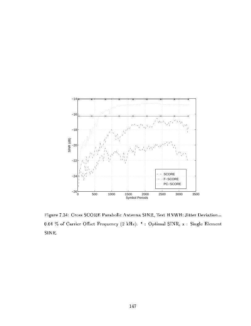
SCORE

F−SCORE

PC−SCORE

0 500 1000 1500 2000 2500 3000 3500−26

−24

−22

−20

−18

−16

−14

Symbol Periods

SIN

R (

dB)

Figure 7.34: Cross SCORE Parabolic Antenna SINR, Test HNWB: Jitter Deviation=


SINR.

147

SCORE

F−SCORE

PC−SCORE

0 500 1000 1500 2000 2500 3000 3500−17

−16

−15

−14

−13

−12

−11

−10

−9

−8

−7

Symbol Periods

SIN

R (

dB)

Figure 7.35: Cross SCORE Parabolic Antenna SINR, Test LNNB: Jitter Deviation=


SINR.

148

When the jitter deviation reaches a threshold dependent on the system noise

power, the averaging of the frequency jitter becomes more sensitive to error. After

a certain averaging time, (500 symbol periods as shown in Figure 7.35), the errors

in the carrier oset eventually result in the SCORE algorithm rejecting the desired

signal.

A similar type of behavior was mentioned by Agee [2], who suggested that a

windowing technique be applied to the received data to improve the robustness of

the SCORE time averaging to frequency error. The resulting trade-o would be a

decrease in convergence rate performance. Eects of windowing, as well as nding

the threshold where the desired signal is rejected due to frequency jitter are areas of

future investigation.

7.11 Frequency Oset Convergence Performance

Errors in frequency oset may arise from a variety of sources including temperature

uctuations, or component mismatches.

The Figures 7.36 to 7.38 show the eects of oset frequency mismatch on the

convergence rate. It can be seen that an increase from a noise power of 40.4 dB to

47.0 dB greatly degrades the performance of the SCORE algorithms.

The periodic nature of the uctuation of the beamforming patterns can be ex-

plained in terms of the frequency rejection nature of the SCORE algorithms. The

algorithm will converge to the desired beamforming weights up until the point where

the time averaging will begin to reject the desired signal. After a sucient averaging

time, (1000 symbol periods for Figure 7.36), the desired signal is completely rejected,

and the convergence to the desired pattern begins again. The reduction in succes-

sive maxima of the SINR is attributed to the increased sensitivity of the SCORE

algorithms to the cyclic frequency error.

The periodic convergence uctuation increases in frequency as the carrier oset

error increases. This can be seen by the quick rejection of the PC-SCORE signal in

149

SCORE

F−SCORE

PC−SCORE

0 500 1000 1500 2000 2500 3000 3500−20

−18

−16

−14

−12

−10

−8

−6

Symbol Periods

SIN

R (

dB)

Figure 7.36: Cross SCORE Parabolic Array SINR, Test LNWB: Frequency Error =

0.04 % of Carrier Oset Frequency (2 kHz). *-: Optimum SINR, x-: Single Element

SINR.

150

SCORE

F−SCORE

PC−SCORE

0 500 1000 1500 2000 2500 3000 3500−20

−18

−16

−14

−12

−10

−8

−6

Symbol Periods

SIN

R (

dB)

Figure 7.37: Cross SCORE Parabolic Array SINR, Test LNWB: Frequency Error =


SINR.

151

SCORE

F−SCORE

PC−SCORE

0 500 1000 1500 2000 2500 3000 3500−26

−24

−22

−20

−18

−16

−14

Symbol Periods

SIN

R (

dB)

Figure 7.38: Cross SCORE Parabolic Array SINR, Test HNWB: Frequency Error =


SINR.

152

Figure 7.37

The performance of the SCORE algorithms under the frequency jitter and the

carrier oset error environments are similar in terms of the mechanism of SINR degra-

dation. The carrier oset error is considered more critical in terms of convergence

performance because the carrier frequency error cannot be averaged out as seen for

the jitter case in Figure 7.34. Windowing the received data points as suggested by

Agee [2] would be expected to improve the robustness of SCORE to this type of error

at the expense of extending the convergence time.

7.12 Direction of Arrival Eect on the Parabolic

Antenna

It was observed that for the parabolic antenna the maximum theoretical gain was

dependent on the direction of arrival of the desired signal. This direction determined

the magnitude of the received signal and was dependent on the dimensions of the

parabolic antenna and the location of the feeds.

For the above test conditions, the direction of arrival of the signal was 4:21

and

the tilt angle was 0:23

. Table 7.1 shows that there are three elements that have a

signicant contribution with this direction of arrival.

Noise power simulations for test condition LNWB were re-run using a dierent

direction of arrival. The received signal at the antenna elements for this new direction

of arrival is displayed below in Table 7.2.

The following graphs show the result of the change of direction of the desired

signal on the theoretical beamforming gain, as well as on the gain of using the single

strongest antenna element.

Figures 7.39 to 7.41 can be compared with gures 7.27 to 7.29. These graphs

show comparable convergence performance for the same signal environment. The

only dierence is in the direction of arrival of the desired signal.

Figure 7.42 shows the converged SINR value after an averaging time of 3000

153

Element Received Received Gain

Number Magnitude Angle (dB)

1 22.71 -10.00 27.12

2 15.35 -9.23 23.72

3 34.66 42.33 30.80

4 0.88 105.07 -1.12

5 4.23 130.51 12.52

Table 7.1: Direction of Arrival Information for the Parabolic Antenna: = 0:23

= 4:21

Element Received Received Gain

Number Magnitude Angle (dB)

1 37.66 -1.75 31.52

2 20.17 0.21 26.07

3 20.03 1.99 26.04

4 27.38 -2.44 28.75

5 20.25 -0.36 26.13

Table 7.2: Direction of Arrival Information for the Parabolic Antenna: = 0:0

= 3:5

154

SCORE

F−SCORE

PC−SCORE

0 500 1000 1500 2000 2500 3000 3500−5.5

−5

−4.5

−4

−3.5

−3

−2.5

−2

−1.5

−1

−0.5

Symbol Perods

SIN

R (

dB)

Figure 7.39: Cross SCORE Parabolic Antenna Performance: = 0

= 3:5

. Re-

ceived SINR=-36 dB. *-: Optimum SINR, x-: Single Element SINR.

SCORE

F−SCORE

PC−SCORE

0 500 1000 1500 2000 2500 3000 3500−20

−18

−16

−14

−12

−10

−8

−6

Symbol Perods

SIN

R (

dB)


= 3:5

. Re-


155

SCORE

F−SCORE

PC−SCORE

0 500 1000 1500 2000 2500 3000 3500−28

−26

−24

−22

−20

−18

−16

−14

Symbol Perods

SIN

R (

dB)


= 3:5

. Re-


156

symbols. Here the optimal and converged gain for the dierent scenarios, as compared

to the single element case, is approximately 4 dB. For the same test conditions (test

condition LNWB) Table 7.30, shows an optimum gain of approximately 2.5 dB due

to beamforming.

The above comparison demonstrates the sensitivity of the performance of the

parabolic antenna system on the the position of the antenna elements and the parabola

geometry. The 1.5 dB dierence between the two scenarios merits an investigation

into the optimization of the antenna element location.

SCORE

F−SCORE

PC−SCORE

38 40 42 44 46 48 50 52

−20

−15

−10

−5


SIN

R C

alcu

latio

n

Figure 7.42: Cross SCORE Steady State SINR Parabolic Antenna Noise Performance:

= 0

= 3:5

. Received SINR=-50 dB. *-: Optimum SINR, x-: Single Element

SINR.

Figure 7.43 shows the beam pattern of the new direction of arrival.

It is important to note that the parabolic antenna array is fundamentally dierent

to the linear array with respect to the maximum beamforming gain possible. Each

element of the linear array receives approximately the same amount of power from

the desired signal. Therefore correct beamforming results in an increase in the signal

power by the multiple of the number of feeds. This can be seen in the linear element

simulation results (Figure 7.8) where the optimal SINR is 7 dB above the single

157

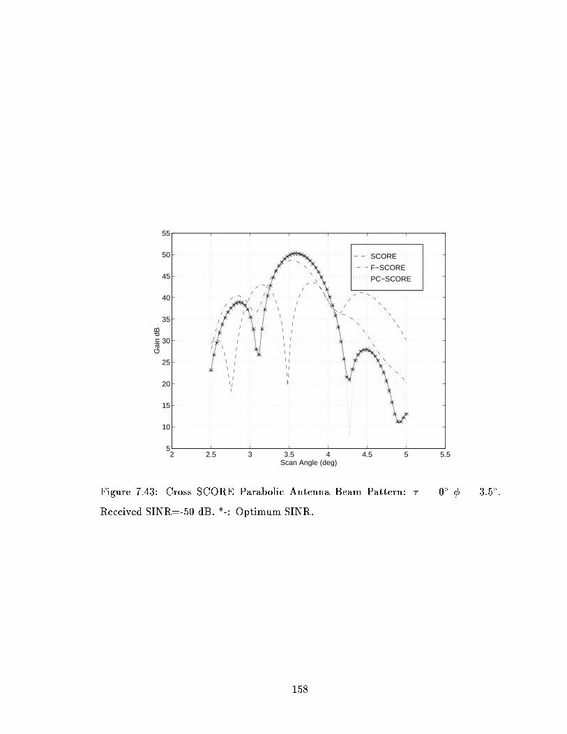
SCORE

F−SCORE

PC−SCORE

2 2.5 3 3.5 4 4.5 5 5.55

10

15

20

25

30

35

40

45

50

55

Scan Angle (deg)

Gai

n dB

Figure 7.43: Cross SCORE Parabolic Antenna Beam Pattern: = 0

= 3:5

.

Received SINR=-50 dB. *-: Optimum SINR.

158

element SINR for a 5 element array.

The parabolic antenna acts like a "physical" beamformer. The re ector coherently

adds the re ected components of the desired signal at a specic location on the feed

plane. Therefore the received power of the desired signal for the parabolic antenna is

dependent on its proximity to the focal point.

The re ector has much the same eect as a beamforming algorithm. A beamform-

ing algorithm multiplies the signal received from dierent feeds by complex weights

such that they add coherently.

Tables 7.1 and 7.2 show that only two or three antenna feeds receive a signicant

amount of power from the desired signal. This results in a maximum gain of only

two to ve dB of beamforming gain depending on the direction of arrival. More gain

would be possible if the feeds were placed closer together on the feed plane, however

there are physical limits to the feed density.

7.13 Performance Summary of Filtered SCORE

Algorithms

The A-SCORE and FA-SCORE implementations show no signicant dierence from

the SCORE and the F-SCORE performance respectively. This is because the initial-

ization of the antenna weights in the A-SCORE and the FA-SCORE play no eect in

the algorithm performance if the time averaged autocorrelation matrix of the signal

environment is poor. Therefore the SCORE algorithm's performance would be best

improved by optimizing the convergence rate as opposed to estimating the direction

of arrival of the signal.

The PC-SCORE algorithm performed best in all conditions tested for the parabolic

antenna array. This algorithm had signicantly faster convergence rates, and showed

convergence at SNR levels of -50 dB. The PC-SCORE technique also had an improved

robustness performance with respect to errors in the carrier oset frequency.

The reason for this improvement is attributed to the reduction of the input noise

159

power to the beamformer, and the preservation of the received signal's phase infor-

mation. The eects of this mechanism are detailed in Section 6.2.3.

The F-SCORE algorithm's performance was dependent on the bandwidth of the

front end lter. There was an optimal lter level observed in the simulations which

depended on the noise environment. The mechanism proposed for this behavior is the

tradeo between the dilation of the noise pulse in the time domain and the reduction

of the noise power. The gains which result from optimization were small, and may

not merit the additional computational expense.

The geometry of the parabolic antenna makes the maximum theoretical gain for

beamforming dependent on the direction of arrival of the signal and the location of

the feeds on the feed plane. This uneven distribution of the signal power on the

feed plane means that only feed elements in close proximity to the focal point of

the desired signal will contribute signicantly to the beamforming gain. This is very

dierent from linear arrays, where each element contributes the same amount to the

beamforming gain.

160

Chapter 8

Conclusions and Future Work

Conclusions on the major areas that this thesis has investigated are presented in this

chapter:

The rst area deals with the modeling of the physical conditions of the satellite

environment. This area includes modeling the satellite channel, design of the

antenna, and simulation of the coverage area.

A summary of the theoretical eects of ltering is presented.

Conclusions reached on the selection of the best SCORE technique and the most

advantageous antenna array are given.

The next section focuses on the performance of the proposed method of calcu-

lating the array response using cyclostationary techniques.

The performance and performance comparison of the front-end ltering tech-

niques with the Cross SCORE and the Least Squares SCORE are presented.

Conclusions are drawn about the convergence rate, and the robustness of each

algorithm.

A nal summary is given on the feasibility of a geostationary satellite channel at

the Ka band frequency using the property of cyclostationarity. In closing, suggested

areas of future work are presented.

161

8.1 Conclusions on the Geostationary Satellite Chan-

nel

The link budget analysis of the satellite channel at the Ka frequency band for the

geostationary satellite system showed that the system was noise limited (Section 3.2).

The major factors contributing to the channel attenuation were the free space loss,

the thermal noise received from the wide message bandwidth, and the attenuation

margin needed to account for changing atmospheric conditions. This is presented in

the FDMA link budget calculation in Table 3.2. The high frequency of the channel

made eects such as ionospheric distortion negligible due to their 1=f dependence

(Section 3.3.12).

It was also noted that since the terrestrial receiver is stationary during transmis-

sion, and the channel uctuations due to weather are slow, a long integration period

for time averaging possible (Section 3.2). This makes the satellite channel potentially

viable for cyclostationary beamforming using a long integration time under high noise

environments.

8.2 Conclusions on Antenna Design

Based on the calculation techniques of this thesis, it is feasible to construct a high gain

parabolic antenna to be used in the satellite link (Section 2.2). Present technology

oers a number of candidates of feed antennas such as the Potter horn, or patch

antennas which would satisfy the requirements of having a broad bandwidth, and

small physical dimensions (Appendix A).

In this thesis an antenna was designed with an on focus gain of 53.4 dB. Re ector

diameters were 1.67 m and 2.50 m for the uplink and downlink antennas respectively.

Focal lengths were 1.21 m and 1.81 m for the uplink and downlink respectively (Table

2.7).

162

8.3 Conclusions on SCORE Algorithm Simula-

tion Performance

The following sections relate the conclusions drawn about the general eect of the

simulated robustness tests performed on the SCORE technique of beamforming.

8.3.0.1 SCORE Noise Performance

The front-end ltering techniques of SCORE improved the convergence rate perfor-

mance of the beamforming system under high noise conditions. A summary of the

conclusions based on the noise simulations of Section 7.8 are presented below:

Beamforming Convergence Rate Performance

The ltered SCORE techniques were shown to improve the convergence rate per-

formance under high noise conditions after a correlation time of 3000 symbol periods.

Filtered SCORE and PC SCORE began to show sub-optimal performance at received

SNR levels of -45 dB and -48 dB under test conditions LNWB (Figure 7.30) and -43

dB and -50 dB for test conditions LNNB (Figure 7.15) respectively.

Optimum SNR Levels

High noise simulation showed that the ltering of the received signal would result

in convergence of the SCORE algorithm to the optimum SNR level, as predicted in

Section 6.2.10.

Optimum SNR levels for the high noise environment including antenna and beam-

forming gains were often below -10 dB for high noise environments (Section 7.8.2).

The bulk of the optimal SNR gain for the simulations came from the antenna re ec-

tor geometry, (31 dB based on Figure 7.30), while only 2.5 dB of beamforming gain

resulted for the worst case direction of arrival scenario (Section 7.8.3). This signal

level is too low for reliable data performance.

For a practical system an additional gain in the optimum performance of 15 to

25 dB would be necessary. This gain could come from an increase in the parabolic

antenna gain, or through the beamforming gain. The beamforming gain could be

163

increased using more antenna feed elements or through dierent antenna geometries.

8.3.0.2 SCORE Interference Performance

At low noise levels, the frequency rejection nature of the cyclostationary algorithms

eliminates most of the eect of the interferer. In the channel environment modeled,

the interfering signals will have a signal power well below the noise power level.

Interference is therefore not expected to have a signicant in uence on the SINR

values. It is for this reason that no signicant eect of ltering was observed in the

interference environment (Section 7.9).

8.3.0.3 SCORE Carrier Oset Jitter Performance

The eect of errors produced in the carrier oset frequency were observed. Based on

dierent magnitudes of the deviation of the uctuation it was observed that there is

a threshold where a particular algorithm will converge to the optimum SINR value.

All algorithms showed a very high degree of sensitivity to this frequency jitter.

Frequency deviations as low as 0.05 % (2.5 kHz) of the normalized sampling frequency

at noise power levels of 40 dB and 12 dB for the parabolic and linear scenarios,

respectively, resulted in a deterioration of SINR level as the averaging time increased

(Section 7.10).

The mechanism for this behavior is based on the ability of the cyclostationary al-

gorithm to correctly estimate the cyclic autocorrelation matrix. This ability degrades

as the jitter increases. Furthermore, the longer the averaging time, the more sensitive

the algorithm becomes to the error in the cyclic autocorrelation matrix. This resulted

in the degradation of the SINR levels past approximately 500 symbol periods for the

test conditions observed.

The noise level signicantly eected the sensitivity of the algorithms to frequency

jitter.

164

8.3.0.4 SCORE Oset Carrier Frequency Error Performance

All algorithms were demonstrated to be very sensitive to any error in the oset carrier

frequency. The performance degradation resulted in a uctuation in the SINR value as

the time averaging period increased and eventually diverged. This periodic uctuation

increased as the oset carrier frequency error increased. The sensitivity to oset error

in the carrier increased as the noise power level increased (Section 7.11).

In this test, the carrier signal appears much like an interferer to the cyclostationary

algorithm which is eventually rejected by the algorithm. The frequency rejection

capability of SCORE was presented in Section 6.2.

8.3.0.5 SCORE Front End Filter Bandwidth Performance

Variations of the bandwidth of the front-end lter did not have a signicant eect

on the convergence of the beamforming algorithms, front end ltering did have the

ability to improve the performance of the SCORE algorithms especially under high

noise environments. Therefore, bandwidth optimization to improve the convergence

rate would be dicult to justify in terms of the computational expense in the test

conditions studied.

Simulation results in relatively low noise environments showed that the SINR

performance curve as a function of the bandwidth was almost at. A wide range

of lter bandwidths could therefore be selected with only a small deterioration of

lter performance from the optimal parameter. Filter bandwidth design becomes

marginally more important as the noise power of the environment increases (Section

7.7.1).

The positive eect of ltering reduces the noise power input into the beamformer.

The draw back is that there is a pulse dilation of the input signal which results is

caused by the nite noise frequency band, and any non-linear phase relationships to

frequency (Section 6.2.3.2). The correlation of the noise terms in the time domain

will result in an increase in the convergence time.

165

The PC-SCORE algorithm removes the non-ideal phase eect, and the perfor-

mance deterioration was not observed for small bandwidths.

It is important to note that ltering only alters the convergence time of the algo-

rithms, and does not aect the nal convergence value. This was explained in Section

6.2 and supported by the simulation results.

8.3.1 SCORE Algorithm Performance Summary

Table 8.1 provides a summary of the SINR performance of the convergence results

presented in Chapter 7. Values of the SINR convergence were taken at 500 symbol

periods and 3000 symbol periods. It is important to note that these selected values

do not indicate the convergence trends over the integration times.

8.4 Conclusions on Array Estimation using Cy-

clostationarity

The relative delay among elements for a known sinusoidal oset carrier was estimated

using cyclostationarity. This information was used to calculate the array response of

the antenna array. The application of array estimation to this thesis was an attempt

at increasing the convergence rate of the SCORE algorithms. As shown in Chapter 7,

estimating the array response did not improve the convergence rate for the SCORE

algorithms under the test conditions chosen.

The eect of bandwidth, carrier frequency jitter, and carrier oset error follow the

same trends as for the SCORE algorithms. The PC-Array algorithm performed the

best, followed by the F-Array algorithm.

166

Test Parameters Opt Single SCORE SINR dB (Symbols)

SINR Feed PC F SCORE

SINR 500 3000 500 3000 500 3000

Comparison: Cross SCORE and Least Squares SCORE

LS N=36, BW=.05 Hz -3.3 -5.5 -3.5 -3.45 -4 -3.4 -3.6 -3.35

CS N=36, BW=.05 Hz -3.3 -5.5 -3.45 -3.44 -3.7 -3.44 -3.45 -3.35

Comparison: Filter Bandwidth

CS N=42, BW=.05 Hz -10.2 -13.3 -10.8 -10.2 -14 -10.8 -14 -11

CS N=42, BW=.2 Hz -10.2 -13.3 -10.8 -10.2 -11.8 -10.3 -14 -10.8

CS N=40, BW=.4 Hz -7.5 -9.6 -8 -7.6 -8.5 -7.6 -8.2 -7.6

Comparison: Noise Power

CS N=36, BW=.2 Hz -3.3 -5.5 -3.4 -3.3 -3.4 -3.3 -3.4 -3.3

CS N=42, BW=.2 Hz -10.2 -13.3 -10.8 -10.2 -11.8 -10.3 -14 -10.8

CS N=50, BW=.2 Hz -17.9 -20 -24.8 -19.2 - - - -

Comparison: Frequency Jitter (Cross SCORE)

LNWB Dev=.04 % Hz -7.5 -9.6 -7.8 -7.6 -8 -7.6 -8.4 -7.8

HNWB Dev=.04 % Hz -14.1 -16.2 -17.5 -14.8 -21 -17 -23 -21

LNNB Dev=.2 % Hz -7.5 -9.6 -7.8 -10.5 -9.5 -13.5 -9.5 -14

Comparison: Frequency Oset Error (Cross SCORE)

LNWB FErr=.04 % Hz -7.5 -9.6 -8 -18 -9 -18 -9.5 -19

WNWB FErr=.2 % Hz -7.5 -9.6 - - - - - -

HNWB FErr=.04 % Hz -14.1 -16 -20 - - - - -

Table 8.1: SCORE SINR Convergence Summary: Parabolic Antenna

167

8.4.1 Conclusions on Cyclostationary Array Estimation for

the Linear Array

The linear array performs well in the estimation of the array response. Convergence

rates based on symbol times are comparable to those of the least squares SCORE

algorithm. All elements converge with approximately the same rate of convergence,

and the convergence rate is independent of which element is chosen as the reference

element.

8.4.2 Conclusions on Cyclostationary Array Estimation for

the Parabolic Antenna

The parabolic antenna was observed to converge to a SINR level close to the SINR of

the single element with the strongest received signal strength for the test conditions

observed. This is well below the optimal level.

The reason for this poor performance arises from the gain of the re ector parabola.

Each element's received signal strength depends upon its location on the feed plane

relative to the direction of arrival of the signal. For this reason the selection of the

reference element for the cyclostationary array estimation is critical. Selection of a

reference element with a weak signal will signicantly harm the convergence rate. This

behavior is conrmed from the convergence plots of the individual array elements.

This dependence on array geometry and direction of arrival makes the cyclosta-

tionary array estimation technique poor for the satellite environment or for parabolic

arrays in general. If some method of selecting the array element with the maximum

desired signal strength could be found, then the dependence on the direction of arrival

of the desired signal would be reduced.

168

8.5 Final System Design Proposal

Based on the simulation results in the previous chapters, and the link budget calcu-

lations, the following sections outline the design of a Ka broad band geostationary

satellite system which uses cyclostationary beamforming. An FDM access scheme is

assumed and no gain derived from coding is included in the link budget.

The system has been left as generic as possible and focuses exclusively on beam-

forming aspects of the link. No reference is made with respect to standards or pro-

tocols. Frequency reuse limits are not investigated. The goal is to provide a feasible

system model that could be developed for a specic standard.

8.5.1 Phase-Compensated SCORE Algorithm

Based on the superior convergence ability and robustness of PC-SCORE (Section

7.13) this algorithm is best suited for Ka band satcom applications. The algorithm

should use a front end lter with a bandwidth of .05 of the sampling frequency.

The PC-SCORE showed a signicant performance improvement over SCORE and

F-SCORE under high noise environments and limited convergence times (Section

7.8). It did not degrade in performance under low lter bandwidth conditions like

F-SCORE (Section 7.7.1).

Based on the convergence rate performance improvement compared to F-SCORE,

the increase in computation required for phase compensation was seen to be justied.

8.5.2 Link Budget

Based on the calculated link budget levels presented in Table 3.2, it is clear that for

the system to have SINR levels required to achieve a bit error rate of less than 10

5

without coding gain and using the design parameters outlined in Table 1.1 is beyond

the ability of the algorithms considered. The received SNR level of the desired signal

(i.e. without the gain of the parabolic antenna) is -100.11 dB and -113.06 dB for the

downlink and uplink respectively.

169

To overcome the noise problem, it is proposed that terrestrial systems use a highly

directive antenna. This solution will increase system cost, and require some method

of pointing the earth station antenna towards the satellite. Since the user is not

expected to be moving during transmission, targeting the satellite is not expected to

be a dicult problem.

Additional methods of increasing the link budget SNR could involve using higher

gain antennas, system designs which result in higher beamforming gains (more an-

tenna elements) or by operating at lower orbits or frequency bands. These techniques

were not pursued in this thesis.

8.5.3 Receiver Antenna

The terrestrial antenna considered to improve the link budget is described in [31].

This antenna is .5 m in diameter, operates from 19 to 29 GHz, with a gain of 38.7 dB

and 42.3 dB respectively. This antenna is ideal for the satellite system application.

8.5.4 Uplink System Limits

Using the antenna gain described in Section 8.5.3, the received power at the satellite

based on the calculations in Table 3.2 would be -74.28 dB. This SNR is beyond the

convergence capability of the beamforming algorithms studied over the 3000 symbol

periods considered. If an optimal beamforming gain of 4 dB could be achieved, then

using a parabolic antenna gain of 48.1 dB the nal SINR would be -22.18 dB which

is 32.18 dB below the SINR needed for a BER of 10

5

. This decit could be made

up by altering the system design.

8.5.5 Downlink System Limits

A method of providing a reference signal from the terrestrial user is required in any

access scheme. This signal is needed to allow the satellite downlink to beamform

on the user. Two methods of providing a reference signal could be achieved either

170

by using a pilot tone, or through frequency scaling the beam weights of the uplink

connection. The potential source of error with frequency scaling is the need for

accurate calibration of the array manifold, and accurate knowledge of the carrier

frequencies being used.

Using a terrestrial antenna design such as the one presented in [31] with a 42.3 dB

gain would result in a received SINR of -57.71 dB at the antenna elements. Assuming

that an optimal beamforming gain of 4 dB could be achieved using a 48.1 dB satellite

antenna, the nal SINR would be -5.61 dB which is 15.61 dB below the SINR needed

for a BER of 10

5

. It is conceivable that a changes in the system design could achieve

the required BER.

In the down link budget, a 15 dB margin was given to atmospheric losses. From

Table D.3 the down link would suer on average only 10 fades of more than 1000

seconds per year and only 100 fades of more than 10 seconds per year.

Link Condition Uplink (dB) Downlink (dB)

Received SINR -112.98 -100.01

Received SINR (Earth Antenna -74.28 -57.71

38.7/42.3 dB Up/Down Gain)

Margin below Beamforming 24.28 7.71

Threshold (-50 dB)

SINR with Satellite -26.18 -9.61

Re ector Gain (48.1 dB)

SINR assuming Optimal -22.18 -5.61

Beamforming (4 dB)

10

5

BER Margin -32.18 -15.61

Table 8.2: SINR Calculations of Proposed Satellite System

171

8.5.6 System Robustness

As shown in Chapter 7 the cyclostationary SCORE algorithms are highly sensitive

to any error in the oset carrier. The requirement for highly accurate oscillators and

hardware modications to limit temperature uctuations etc. on the satellite and the

receiver would greatly increase the cost of the system. It is unclear that even these

modications would ensure reliable performance. Other techniques such as frequency

tracking may over come this problem.

8.5.7 Proposed System Specication Modications and Per-

formance Observations

The specications for this thesis were chosen based on geostationary satellite com-

munications systems which operated at lower frequencies and at lower bandwidths.

The link budget calculations show that parabolic antenna beamforming alone cannot

achieve the E

b

=N

o

required for data rate service. Additional gain will have to be

provided using coding, power, or bandwidth trade-os.

The investigation of the Ka band geostationary satellite link using parabolic beam-

forming did reveal several important areas to be considered in future system designs

(Chapter 7). The satellite channel for a broadband service at the Ka frequency band

was shown to be noise limited. The SCORE algorithms were modied to work under

high noise environments. Finally, the limited application of the parabolic antenna to

beamforming was characterized.

8.6 Suggested Future Areas of Investigation

In this thesis many aspects of cyclostationarity were investigated through simulation.

Where possible, theoretical explanations were oered to explain the trends observed,

however the focus of the thesis was more on establishing the important parameters af-

fecting the performance of the cyclostationary algorithms in high noise environments.

The following sections are a list of some of the areas which merit further investigation.

172

8.6.1 Channel Simulation Model

Investigation into wireless satellite communications at the Ka band is an area of

ongoing research. The calculations used in this thesis combined statistical models,

with empirical data from the most up to date sources available. Since this area

of research constantly being updated, any future application of beamforming to Ka

satellite communications must keep current with new research.

8.6.2 Antenna and Feed Plane Design

The antenna designed in this thesis was accurate to rst order eects. Increased gains

in antenna eciency and performance designs may be possible using more advanced

design tools which were not available to the author.

Antenna eects which should be more thoroughly investigated included element

coupling, and optimization of inter-element distance to produce maximum gain (Sec-

tion 2.3.6).

Techniques need to be investigated to maximize the gain of the received signal

while minimizing the number of elements, and eect of user location on beamforming

performance. These gains would depend on the pattern of the feeds on the feed plane,

and antenna beam width optimization.

8.6.3 Noise Performance Limit

The beamforming ability of the dierent SCORE algorithms should be characterized

with respect to noise performance. Simulation results indicate that the dierent algo-

rithms begin to degrade at a certain received SNR level. The factors which contribute

to this degradation threshold should be characterized in terms of the channel, and

the lter specications.

173

8.6.4 Interference Performance

It was shown that the presence of a single interferer in a noise limited environment

does not signicantly aect the performance of the algorithms. The eect of the

interference on the convergence of dierent algorithms should be investigated for

lower levels of noise power relative to the desired signal power and interference power.

While this characterization is not relevant to this satellite channel model, it would be

relevant to terrestrial systems or satellite systems operating at lower frequencies.

8.6.5 Frequency Jitter Performance

Simulations showed a high degree of sensitivity of the algorithms to frequency jitter

at the cyclostationary frequency. Research in this area should focus on more realistic

models of frequency jitter. Techniques which may make the algorithms more robust

to jitter should also be investigated. This might include methods of weighting the

values of the received signal samples based on the time of arrival.

It was also observed in the simulations that there might be a threshold at which

the algorithms investigated will converge to a stable level. This threshold appears

to depend on the noise power level, as well as the jitter deviation. A theoretical

explanation of this behavior should be investigated.

8.6.6 Oset Frequency Error

All algorithms were very sensitive to any error in the oset cyclostationary frequency.

This was noted by a periodic uctuation of the SINR which depends on the magnitude

of the frequency error. A relation between the frequency error, noise power level, and

magnitude and period of the SINR uctuations should be investigated.

8.6.7 Filter Optimization

Only one lter type was investigated in this thesis. Dierent parameters for the

transitional lters should be investigated, as well as other lter types which trade o

174

attenuation with phase distortion.

Section 6.2 oers an explanation as to the mechanism of how ltering is advan-

tageous to beamforming in high noise environments. This model should be explored

further to characterize the signicance of the phase errors and noise power reduction

introduced by the lter. Such a relation could possible oer a method of adaptively

selecting an optimal lter bandwidth depending on the noise conditions.

8.6.8 Cyclostationary Array Estimation

Theoretical relationships for the performance of the proposed cyclostationary array

estimates should be found. This would include the eect of the convergence rate with

the selection of reference elements with varying signal strengths, robustness and the

sensitivity of the array estimation with respect to the error in the calculated array

response. This result would indicate to which environment this array estimation

technique could be applied.

The binary search algorithm used to nd the delay among elements is simple but

lacks robustness. The performance of the cyclostationary array estimation may be

improved by a more robust technique, and one that converges faster.

A method of estimating the antenna element with the highest received power

of the desired signal should be found. This would minimize the dependence on the

parabolic conguration on the direction of arrival of the desired signal, and is expected

to improve the convergence rate performance.

8.6.9 Low Earth Orbit Satellite Applications

The large amount of attenuation which results from the geostationary orbit is a major

cost in the link budget calculation. A low earth orbit application may improve the

link budget, and make the satellite system more robust. There would be an increase

in complexity in the system which would require tracking of the target location due

to the asynchronous orbit of the satellite with the earth.

175

8.6.10 Terrestrial Applications

The linear array as well as the least squares SCORE technique showed convergence

trends at lower noise power levels. An investigation should be made into the appli-

cation of these techniques to lower noise environments such as for terrestrial applica-

tions. Terrestrial applications would require simpler algorithms and array congura-

tions which are satised by the least squares SCORE and the linear array respectively.

8.6.11 Algorithm Optimization

This thesis neglected any attempt to calculate the computational complexity of the

algorithms. To complete the investigation, more cyclostationary beamforming tech-

niques should be compared to the SCORE methods presented here on the basis of

convergence and complexity. In particular, the sub-space constrained SCORE tech-

niques should be compared to the front end ltering techniques. It is expected that

constraining the weight vector to the signal sub-space will have a similar eect as

front end ltering.

176

Appendix A

Antenna Design and Simulation Methods

This appendix outlines the methods followed to calculate the oset parabolic antenna

used in the link budget calculation and the beamforming simulation of the satellite

system. Background on antenna feed elements and lter design methods are also

presented.

A.1 Calculation of the Oset Parabolic Re ector

Dimensions

The formulas for the design of a Parabolic Re ector are give by Lee and Rahmat-

Samii. [26] They can be used to provide approximate dimensions for a parabolic

antenna which satises certain parameters. These dimensions may then be modied

using a more accurate antenna simulation program developed by Duggan to meet the

exact specications. Figure A.1 shows the design geometry for the oset re ector

antenna.

The basic equation for the parabolic re ector surface can be found using:

z =

x

2

+ y

2

4F

F (A.1)

The feed radiation pattern is modeled for oset feeds using:

g(

0

) = (cos(

0

))

q

(A.2)

177

xa

Ω1

Ω2

Ω3

za

h1

D1

xa

ya

A

D/2

h

l

Aperture

ant

ant

F

Parent Parabola

ReflectorParabola

Figure A.1: Oset Parabolic Antenna Schematic

q =

log(14)

log(cos(

1

2

(

2

1

)))

(A.3)

The feed employed in the thesis is symmetric in its electric and magnetic components.

4 is the aperture taper.

The edge taper (ET) is used to measure the electromagnetic distribution of radi-

ation across the re ector. This quantity may be used to nd the antenna's eciency.

ET = j20 log

10

(14)j (A.4)

The geometry of the re ector is completely determined by the focal length, the re-

ector diameter and the oset height. To arrive at these dimensions, the following

design information must be given.

The sidelobe level of the secondary pattern must be determined.

The half power beamwidth must be dened.

The maximum scan angle in the z-y, and z-x plane must be calculated.

The oset height of the re ector must be decided.

Calculated and specied parameters must satisfy the following conditions in order

for the equations which are presented to be valid.

178

0 < 4 < 0:85

0 < GL < 3

(

F

D

) < 1:5

3

< 30 deg

3

tan(

3

)

A.2 Design Procedure

The following steps outline the design procedure for nding the geometry of the oset

parabola according to [26]

The aperture taper is found using the following equation:

4 =

3

X

n=0

n

(

SL

10

)

n

(A.5)

The coecients for the oset feed location are:

0

= -8.87

1

= 9.32

2

= -3.00

3

= 0.32

The aperture eciency for the oset feed location may be determined graph-

ically based on the edge taper value (ET) or the aperture taper (4). The

optimum eciency occurs at an edge taper value of 11.00 dB [26].

The diameter for the parent parabola is calculated below. The re ector parabola

is the circular portion of the parent parabola to which the feed plane is directed.

D

1

=

1

sin(

1

)

3

X

n=0

n

4

n

(A.6)

D = 2(h

1

+D

1

) (A.7)

The coecients used in calculating the diameter are:

0

= 1.61

1

= 0.57

2

= -1.43

3

= 1.47

179

The focal length of the antenna is determined by the allowable gain loss (GL)

and the furthermost scan angle

1

. This length may be found for gain losses

less than 3 dB using

F

D

=

(sin(

3

)= sin(

1

))

190 cos

1

[1 (GL=5)]

(A.8)

k = 1 exp(0:12

q

D

1

=) (A.9)

The length from the re ector focus to the re ector center is given by:

l = F [1 + (

h

2F

)

2

]

1

2

(A.10)

The required angles needed for subsequent calculations including the angle and

orientation of the feed plane may be obtained using:

1

= (

h

1

F

)[1

1

4

(

h

1

F

)

2

]

1

(A.11)

2

= (

D

2F

)[1

1

4

(

D

2F

)

2

]

1

(A.12)

3

= (

h

F

)[1

1

4

(

h

F

)

2

]

1

(A.13)

The actual direction of the beam aimed at the focus is altered slightly due to

the re ector geometry. The amount that the beam deviates from the true ray

is determined by the Beam Deviation Factor (BDF) It may be calculated as

follows:

BDF = [1 :72 exp(3:2

F

D

1

)] (A.14)

=

cos(

3

) + cos(

3

1

)

1 + cos(

3

1

)

(A.15)

2

=

1

2

tan

1

[(BDF )

d

l

] (A.16)

Where

2

is the actual direction of the ray. d is the element spacing on the feed

plane.

180

The criteria to insure no feed blockage is to specify the height of the oset

re ector such that the lower edge of the re ector clears the feed array plane.

This condition is satised if

h

1

> d

maxjant

[1 (

h

l

ant

)

2

]

1

2

(A.17)

In order to determine the number of elements required for the antenna feed, the

following calculation is performed. [33]

N

Area

2764(=D

1

)

2

(A.18)

The area is calculated in terms of degrees squared and represents a circular disk

dened by the maximum scan angle

max

. The elements are assumed to be placed in

a hexagonal pattern.

The maximum size of the feed element aperture can be calculated using Equation

(A.19) [33]. This formula is based on the need for low cross polerization levels for a

multiple beam antenna. The result was derived for circular polerization using horn

feeds and giving cross polerization levels below 20 dB. The numbers generated by

this formula will be used as a guideline for antenna element spacing. This feed size

approximation assumed Potter horn feeds which provided low cross polar radiation

levels in the antenna designed in [33].

d

1:25 (F=D

1

) (A.19)

A.3 Approximate Radiation Pattern

The following formula presented in [26] can be used to approximate the radiation

pattern produced by the calculated re ector geometry. The patterns calculated using

matlab were found to produce a radiation pattern close to the design parameters

specied. The nal radiation pattern used in the model system will be calculated

from [11]. The variable

0

ranges from 0 to 2.

181

g(u) =

1

1 0:54

(

2J

1

(u)

u

+4[

2J

2

u

2

2J

1

(u)

u

]) (A.20)

u = D

1

sin(

0

) (A.21)

A.4 Antenna Pattern Program

To accurately perform beamforming calculations, it was necessary to get a more de-

tailed calculation of the antenna beam pattern. It was necessary to nd a program

that would accurately account for design parameters such as feed location, feed po-

lerization, feed plane geometry, and which would accurately calculate the electrical

and magnetic elds based on physical equations.

This program was provided by Duggan in his master's thesis [11], and has been

used with his permission. The program was modied to allow the selection of a tilt

angle which would give beam pattern calculations in a direction o the horizontal

plane of the satellite antenna. Below is a brief summary of the principles upon which

the program was developed. For an account of the formulas used, refer to [11]

A.4.1 Parabolic Antenna Theory and Approximations

The electric eld pattern is found through the solution of the radiation integral.

This integral is simplied using far eld approximations. The program numerically

calculates the integral using the Fourier-Bessel Method.

In order to model the scattering of the electric eld on the parabola, the physical

optics approximation is used. This assumes that scattering takes place as if there was

an innite tangential plane at the point of intersection of the antenna. It has been

shown that this method is accurate for the main beam, but the accuracy decreases

for successive sidelobes.

182

A.4.2 Parameter Specication

The following parameters must be specied to calculated the antenna's radiation

pattern.

Focal length Radius of parabola

Oset height Number of feeds

Polerization Magnitude X Polerization Magnitude Y

Phase oset of Polerization Number of iterations (2

)

Order of Bessel Function

Table A.1: Antenna Parameters for the Oset Parabolic Antenna Program

These parameters are selected based on the system to be simulated, and through

the geometric calculations based on the specications as computed by the simplifying

formulas presented in [26]. The output of the antenna program is compared to the

desired specications and modications are made to meet the original specications.

Dimensions are also bounded by the physical limits of existing systems referenced in

the literature search.

Feed plane X coordinate Feed Plane Y coordinate

Angle with Antenna X Axis () Angle with Y Axis ( )

Angle with Antenna Z Axis () Electric eld Directivity of feed

Magnetic eld Directivity of feed

Table A.2: Feed Parameters for the Oset Parabolic Antenna Program

A.5 Feed Design

A design of an antenna feed that would accurately model all of the electromagnetic

properties is beyond the scope of this thesis. Instead, some of the more signicant

design considerations are presented, along with some references from specic satellite

projects.

183

The antenna feeds needed in this thesis will have to support a frequency range

of approximately 2 GHz. The transmit frequency will be either 20 or 30 GHz. This

requires that the feed have a frequency bandwidth of 10% and 6.7% respectively. It

is also necessary that the feeds be small in size to allow for a large antenna gain while

insuring thorough coverage of the proposed service area. Using recent developments

in microwave technologies and the formulas presented in [33], these goals can be

achieved.

A.5.1 Maximum Theoretical Eciency of Multiple Beam

Antennas

The electromagnetic interaction of the antenna feed matrix causes mutual interference

which can limit the eciency of the overall antenna. In the paper by DuFort [10] he

shows that the maximum eciency for a multiple beam antenna is approximately 50

% for large antenna arrays. This proof is based on the Stein Limit [39] which shows

that the maximum eciency possible is the ratio of the average to the peak value of

the aperture power distribution. [10] shows this to be approximately 50 %. DuFort

goes on to prove that the eciency limit can be achieved by selectively attenuating

the signal in the aperture.

In the antenna feed plane design for this thesis, the maximum eciency is assumed

to be achieved and the limit of 50 % eciency is used in the link budget calculation.

The specic details in the feed design to achieve the 50 % limit are not derived. For

more detail on optimal feed plane eciency design, [10] may be referenced.

A.5.2 Beamwidth of Antenna Feed Elements

Antenna feed elements have a characteristic bandwidth of operation. As a result, it

was necessary to insure that today's technology could provide antenna elements that

could operate at Ka band frequencies, while providing a bandwidth that would allow

complete recovery of the message signal for processing.

184

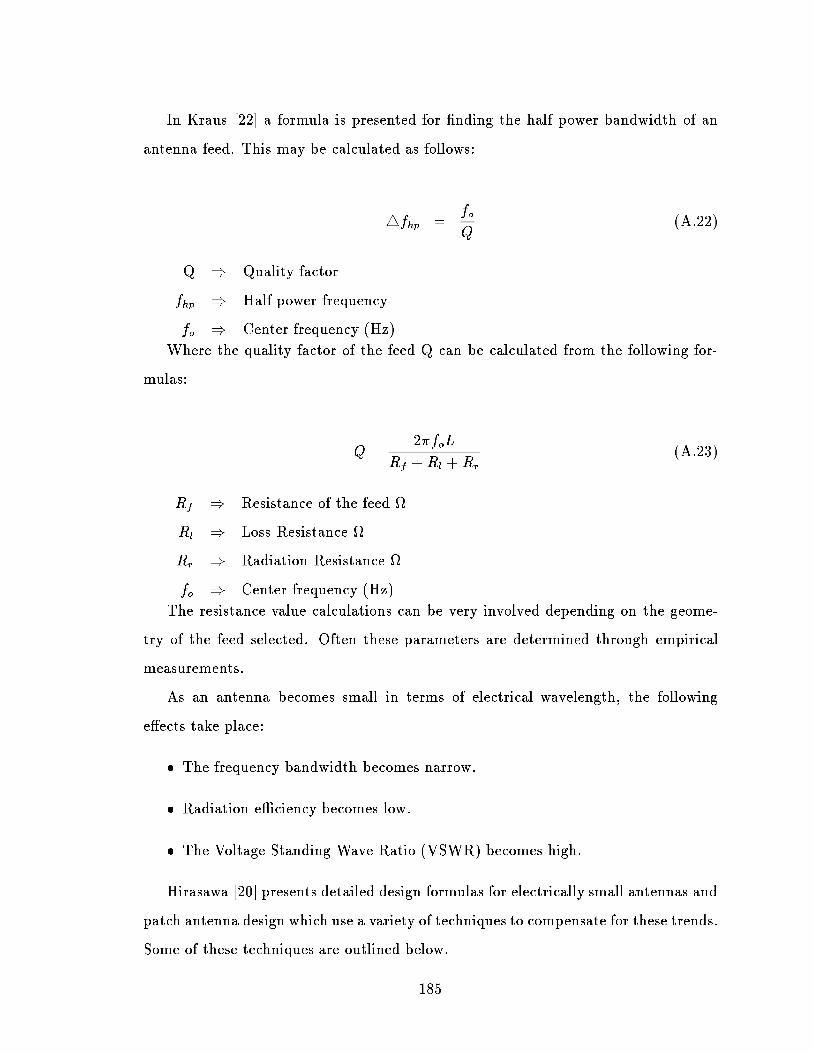
In Kraus [22] a formula is presented for nding the half power bandwidth of an

antenna feed. This may be calculated as follows:

4f

hp

=

f

o

Q

(A.22)

Q ) Quality factor

f

hp

) Half power frequency

f

o


Where the quality factor of the feed Q can be calculated from the following for-

mulas:

Q =

2f

o

L

R

f

+R

l

+R

r

(A.23)

R

f

) Resistance of the feed

R

l

) Loss Resistance

R

r

) Radiation Resistance

f

o


The resistance value calculations can be very involved depending on the geome-

try of the feed selected. Often these parameters are determined through empirical

measurements.

As an antenna becomes small in terms of electrical wavelength, the following

eects take place:

The frequency bandwidth becomes narrow.

Radiation eciency becomes low.

The Voltage Standing Wave Ratio (VSWR) becomes high.

Hirasawa [20] presents detailed design formulas for electrically small antennas and

patch antenna design which use a variety of techniques to compensate for these trends.

Some of these techniques are outlined below.

185

A.5.3 Wide Band Techniques for Antenna Feeds

A.5.3.1 Patch Antenna

The patch antenna is typically characterized by a ground plane covered with a dielec-

tric material. A conductor is placed on top of the substrait in accordance to some

design specication A.2. The dimensions of the patch antenna can be of the order of

a wavelength or smaller.

Dielectric Material

Ground Plane

Conductor

L2

1L

Ground Plane

Short-Circuit Plate

W

Planar Element H

Patch Antenna

Planar F Antenna

Figure A.2: Simple Diagram of a Patch and Planar F Antenna

The patch antenna has the following advantages, depending on the design chosen:

186

[20]

Low prole and conformal structure.

Suitable for mass production (low cost).

Easy for miniaturization and light weight.

Structurally robust.

Integration of a radiator and feeding system is possible.

The standard bandwidth of a patch antenna is 1 - 2 %. [20]

The small size and light weight of the patch antenna make it a good candidate

for a satellite antenna feed, and the oset design of the parabolic antenna would

overcome the interference of the received signal which might be caused by the feed

plane. The standard patch antenna would have a bandwidth that is several percent

too small for the broadband application, however [20] presents methods for increasing

the patch antenna bandwidth. Some of these techniques are presented below.

Low Unloaded Q Substraight:

By selecting a substraight that results in a low Q value, the band width of the

patch antenna may be increased to approximately 8.75 % of the modulating

frequency.

Double Resonance Phenomenon

This technique uses a parasitic element to creat a second resonant frequency.

The result is an increase in bandwidth of up to 8.5 % of the modulating fre-

quency.

Wideband Impedance Matching Network.

Through the use of transmission line broadband impedance matching techniques

the bandwidth of the patch antenna can be increased to 9.1 % of the modulating

frequency.

187

To increase these bandwidths further, a combination of techniques can be em-

ployed.

A.5.3.2 Planar Inverted F Antenna

The Planar inverted F typically consists of a rectangular planar element, ground

plane, and a short circuit plate [20] (Figure A.2). These antennas are low prole, and

have been designed for various portable communication applications.

This type of antenna can be designed to have dimensions less than a wavelength.

The bandwidth of the antenna can be increased by increasing the height dimension

up to a maximum of 14% of the modulating frequency.

A.5.3.3 Planar Spiral Antennas

The text by Elliott [12] contains the design formulas for planar spiral antennas. These

antennas provide a very large bandwidth and a low prole by using micro strip tech-

niques. The drawback is that the antenna's physical dimensions are large, which may

make dense clustering of feeds dicult.

A.5.3.4 Potter Horn Antenna

In the work done by Rao et. al. [33] a 45 GHz multi-beam antenna was designed.

The design used 121 Potter horn feeds to achieve coverage in an 8

diameter. Physical

modeling and theoretical calculations showed that the system operated well within

43.5 to 45.5 GHz. This corresponds to 4.5 % of the modulation bandwidth. The the

Potter Horn antenna can achieve a 30 dB side lobe level of suppression which makes

it a good candidate for the feed antenna required.

A.6 Filter Implementation

It is expected that the satellite system will be noise limited, and therefore selective

ltering is expected to improve the performance of the system.

188

Two lter designs operating on two parallel branches are required. The rst

branch will lter out all noise and message components except for the known carrier

frequency. This path will be used for calculating the antenna weights based on the

cyclostationary properties of the carrier. A schematic of the proposed scheme can be

referred to in A.3

From Feed

and Down Converters

Message Filter(Wide Bandwidth)

Carrier Filter(Narrow Bandwidth at the Carrier Frequency)

To Message Recovery

Hardware

To Beamforming

Hardware

Figure A.3: Broad and Narrow band Filter Schematic for Message and Carrier Re-

covery

The second lter will be a wide band lter, which will pass only the information

on the desired channel. This ltered branch will be used to recover the message data.

Either lter may be implemented using analogue or digital techniques, depending on

the resources available on the satellite. The chosen lters must also preserve phase

information necessary for beamforming and signal combining as much as possible

while providing a large attenuation in the stop band.

The critical lter for the investigation of beamforming is the lter on the cyclosta-

tionary branch. The message lter is expected to improve performance of the system

through out of band noise rejection, but would not aect the performance of the cy-

clostationary algorithms. For this reason, only the cyclostationary lter is designed

and simulated in this thesis.

A transitional lter will be used to achieve the tradeo between passband and

189

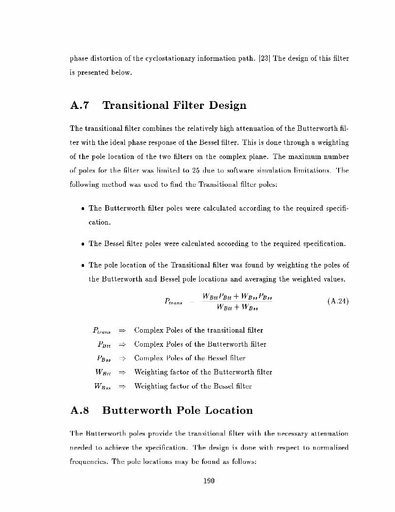
phase distortion of the cyclostationary information path. [23] The design of this lter

is presented below.

A.7 Transitional Filter Design

The transitional lter combines the relatively high attenuation of the Butterworth l-

ter with the ideal phase response of the Bessel lter. This is done through a weighting

of the pole location of the two lters on the complex plane. The maximum number

of poles for the lter was limited to 25 due to software simulation limitations. The

following method was used to nd the Transitional lter poles:

The Butterworth lter poles were calculated according to the required speci-

cation.

The Bessel lter poles were calculated according to the required specication.

The pole location of the Transitional lter was found by weighting the poles of

the Butterworth and Bessel pole locations and averaging the weighted values.

P

trans

=

W

Btt

P

Btt

+W

Bss

P

Bss

W

Btt

+W

Bss

(A.24)

P

trans

) Complex Poles of the transitional lter

P

Btt

) Complex Poles of the Butterworth lter

P

Bss

) Complex Poles of the Bessel lter

W

Btt

) Weighting factor of the Butterworth lter

W

Bss

) Weighting factor of the Bessel lter

A.8 Butterworth Pole Location

The Butterworth poles provide the transitional lter with the necessary attenuation

needed to achieve the specication. The design is done with respect to normalized

frequencies. The pole locations may be found as follows:

190

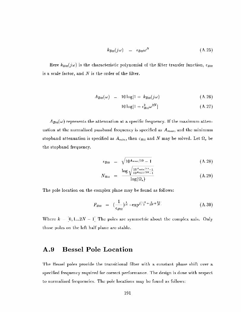
jk

Btt

(j!)j =

Btt

!

N

(A.25)

Here k

Btt

(j!) is the characteristic polynomial of the lter transfer function,

Btt

is a scale factor, and N is the order of the lter.

A

Btt

(!) = 10 log[1 + jk

Btt

(j!)j (A.26)

= 10 log[1 +

2

Btt

!

2N

] (A.27)

A

Btt

(!) represents the attenuation at a specic frequency. If the maximum atten-

uation at the normalized passband frequency is specied as A

max

, and the minimum

stopband attenuation is specied as A

min

, then

Btt

and N may be solved. Let

s

be

the stopband frequency.

Btt

=

q

10

A

max

=10

1 (A.28)

N

Btt

=

log

r

10

A

min

=10

1

10

A

max

=10

1

log(

s

)

(A.29)

The pole location on the complex plane may be found as follows:

P

Btt

= (

1

Btt

)

1

N

exp

j[

2

+

2N

+

k

N

]

(A.30)

Where k = [0; 1:::2N 1] The poles are symmetric about the complex axis. Only

those poles on the left half plane are stable.

A.9 Bessel Pole Location

The Bessel poles provide the transitional lter with a constant phase shift over a

specied frequency required for correct performance. The design is done with respect

to normalized frequencies. The pole locations may be found as follows:

191

The Bessel transfer function is

H

Bss

(s) =

a

o

M

Bssj2

+N

Bssj2

(A.31)

4

= M

Bss

(s) +N

Bss

(s) (A.32)

M

Bssj2

(s) = q

0

+ q

2

s

2

+ ::: (A.33)

N

Bssj2

(s) = q

1

s

1

+ q

3

s

3

+ ::: (A.34)

M

Bss

(s) =

q

0

M

Bssj2

(s)

M

2

Bss

(s)N

2

Bssj2

(s)

(A.35)

N

Bss

(s) =

q

0

N

Bssj2

(s)

M

2

Bss

(s)N

2

Bssj2

(s)

(A.36)

The quantity of interest in the Bessel lter is the delay over the passband which is

ideally uniform. The delay may be calculated using the following formula:

Bss

(!) =

M

Bss2

(!)N

0

Bss2

(!)N

Bss2

(!)M

0

Bss2

(!)

M

2

Bss2

(!)N

2

Bss2

(!)

(A.37)

Where the prime denotes dierentiation with respect to !. The solution to the above

equation for delay may be approximated using Bessel polynomials from which the

Bessel lter poles may be found.

192

Appendix B

Satellite Footprint Calculations

The satellite footprints are contour plots of lines of equal power which originate from

the satellite and intersect the earth. This information is needed to determine the

location of the feed element with the appropriate coverage area on the ground. A

simple method of calculating the main lobe footprints of a geostationary satellite was

derived by Spy and Haakinson [38]. The the technique is limited by the following

restriction.

No consideration is given to the interaction of antenna radiation with atmo-

sphere.

The small variation of received power due to slightly diering distances from

the dierent transmitter locations within a footprint are ignored. This power

variation is due to the curvature of the earth, and is small for small beam

footprints.

The earth is assumed to be perfectly spherical.

Only the main lobe pattern is calculated.

This technique requires knowledge of the satellite longitude location

es

, the aim

point location (

eA

;

eA

), and the beam width

bw

. The program nds a cone of

constant power density which corresponds to the main lobe of the antenna pattern.

193

Once this cone is dened from the satellite position , a locus of intersection of points

with the earth are calculated.

The satellite location for geosynchronous orbit is dened as

s = (

GMP

2

4

2

)

1

3

(B.1)

= 6:62R (B.2)

The formulas required for the calculation of the intersection of a line from the

satellite with the earth are presented below. The beam footprint was found by itera-

tively performing the calculation for the beam for dierent

bw

values.

ye

xe

θbw

φbw

|d |2

|d |1

A

A’

F

S

ze

ρ ρ

T

eA

T

µ

µ

µef

eA

ea

ef

zx

y

aa

a

t

s

f

Figure B.1: Earth-Satellite Geometry for the Calculation of Beam Footprints

194

The coordinate system used for the earth is specied in Appendix E. All dis-

tances are expressed in earth radii.

The aim point is the point on the earth to where the satellite's z axis is directed.

The satellite geometry and orientation relative to each other are specied in

Appendix E. The aim point is a know location on the earth and corresponds to

the beam center for a particular antenna element.

As seen in the diagram B.1, the intersection point of the satellite ray with the

earth may be found by solving the following relation.

~

f = ~s+

~

t (B.3)

Where

~

f is the intersection point of the ray from the satellite with the earth,

~

t

is the ray from the satellite to the intersection point F, and ~s is the ray from the

earth center to the satellite. In this equation the only unknown is the vector

~

t.

For the calculation of the unknown parameters d

1

, d

2

, and

~

t the following proce-

dure is used.

Applying the cosine law to the satellite geometry, it can be shown that:

d

1

= [jsj

2

+ jsj cos

2

(

ea

) cos(

ea

es

)]

1=2

(B.4)

d

2

= [jsj

2

+ 1 2jsj cos

2

(

ea

) cos(

ea

es

)]

1=2

(B.5)

From these values the components of

~

t may be calculated in the earth centered

coordinate system.

t

x

t

=

1

d

1

d

2

[(cos(

ea

) cos(

ea

) jsj cos(

es

)) (B.6)

(d

2

cos(

bw

) sin(

ea

) sin(

bw

) cos(

bw

)) +

(cos(

ea

) sin(

ea

) jsj sin(

es

)) (d

1

sin(

bw

) sin(

bw

))]

t

y

t

=

1

d

1

d

2

[(cos(

ea

) sin(

ea

) jsj cos(

es

)) (B.7)

195

(d

2

cos(

bw

) sin(

ea

) sin(

bw

) cos(

bw

))

(cos(

ea

) cos(

ea

) jsj cos(

es

)) (d

1

sin(

bw

) sin(

bw

))]

t

z

t

=

1

d

1

(sin(

ea

) cos(

bw

) + (d

2

sin(

bw

) cos(

bw

)) (B.8)

To nd the magnitude of

~

t, it can be shown that

~

f

~

f = (~s+

~

t) (~s+

~

t) (B.9)

= 1

This leads to the following quadratic equation:

jtj

2

+B

1

jtj+B

2

= 0 (B.10)

The constants B

1

and B

2

may be found by:

B

1

=

2jsj

d

1

d

2

[(cos(

ea

) cos(

ea

es

) jsj) (B.11)

(d

2

cos(

bw

) sin(

ea

) sin(

bw

) cos(

bw

)) +

(d

1

cos(

ea

) sin(

ea

es

) sin(

bw

) sin(

bw

))]

B

2

= jsj

2

1 (B.12)

The following physical situations occur under these range of values for the discrimi-

nant of equation B.10.

The beam from the satellite does not intersect the earth at all when

B

2

1

4B

2

< 0 (B.13)

This solution gives a complex solution to the equation for

~

t.

The beam from the satellite intersects the earth at two locations when

B

2

1

4B

2

> 0 (B.14)

The smaller magnitude of the two possible solutions corresponds to the physical

projection of the satellite contour on the earth.

196

In conclusion, the Cartesian and angular coordinates for the intersection point f

in earth center coordinates can be calculated using:

f

ex

= s

ex

+ (

t

x

jtj

)jtj (B.15)

f

ey

= s

ey

+ (

t

y

jtj

)jtj (B.16)

f

ez

= (

t

x

jtj

)jtj (B.17)

ef

= tan

1

(

f

z

(f

2

x

+ f

2

y

)

1

2

) (B.18)

ef

= tan

1

(

f

y

f

x

) (B.19)

Computer simulation programs have been created which uses this technique for

nding the beam footprints. For the circular aperture, the variable

bw

ranges over

2 radians, which results in a closed contour of points of intersection with the earth

for a specied beamwidth

bw

and target location A

T

.

197

Appendix C

Beam Patterns for O Focus Feeds

This appendix presents the degradation which results from moving the feed from the

center of the focus. The feed locations were based on the coordinates in table 2.9.

The beam patterns were calculated using the parabolic antenna program developed

in [11].

0 0.5 1 1.5 2 2.5 3 3.5 4 4.5 50

10

20

30

40

50

60Magnitude

Deg

Mag

nitu

de in

dB

Figure C.1: Beam Pattern of Feed 1

198

0 0.5 1 1.5 2 2.5 3 3.5 4 4.5 50

10

20

30

40

50

60Magnitude

Deg

Mag

nitu

de in

dB


0 0.5 1 1.5 2 2.5 3 3.5 4 4.5 50

10

20

30

40

50

60Magnitude

Deg

Mag

nitu

de in

dB


199

0 0.5 1 1.5 2 2.5 3 3.5 4 4.5 50

10

20

30

40

50

60Magnitude

Deg

Mag

nitu

de in

dB


0 0.5 1 1.5 2 2.5 3 3.5 4 4.5 50

10

20

30

40

50

60Magnitude

Deg

Mag

nitu

de in

dB


200

0 0.5 1 1.5 2 2.5 3 3.5 4 4.5 50

10

20

30

40

50

60Magnitude

Deg

Mag

nitu

de in

dB


201

Appendix D

Communications Model Background

This appendix gives a detailed account of the models used in determining the param-

eters to be used in the link budget analysis, and the eects of dierent variables on

the attenuation models used. Only the most signicant of these eects are presented

in the nal calculation for the link budget.

The recent interest in satellite communications using the Ka frequency band has

lead to a study of the eects of atmospheric conditions on the propagation of these

service links. Empirical studies have revealed a lot of variation among sites, due

to variables such as temperature, elevation angle, relative humidity and other site

specic phenomenon. Much has yet to be satisfactorily modeled.

The atmospheric communication link for this thesis has been developed based

primarily on the empirical statistical data collected by Loo [27], and the Olympus

Satellite experiment performed by Warren et.al. [42], the CCIR model, and the mod-

els presented by Allnutt [3] which are developed using experimental and theoretical

calculations.

Atmospheric attenuation due to Ionospheric conditions, Tropospheric conditions,

and Rain attenuation were investigated. Where possible, other atmospheric eects

were incorporated into the model based on the data available. Channel modeling

of the Ka band is an area of on going research, and there is relatively little long

term empirical data available which can be used for simulation. The channel model

presented here incorporates the most signicant in uences on the Ka band frequency

202

link, and where possible pessimistic values were used to give a upper bound on the

attenuation. Other factors are omitted from the model and the justication for these

omissions are presented.

D.1 Statistical Channel Model of the Carrier at

the Ka Frequency Band

In order to determine the conditions under which the beamforming algorithms must

perform, it is rst necessary to develop an accurate channel model. The goal of this

model is to predict the amount of attenuation of the signal at the Ka frequency band,

and the necessary gain needed to achieve the system goals. This information will also

be used in designing the parabolic antenna used to receive the signal.

The paper by Loo [27] collects signal strength and phase measurements from the

Olympus satellite for both mobile and stationary signals. The test measurements

were taken from the region around Ottawa Ontario Canada. This locality had an

elevation angle of 14:2

with respect to the satellite. A continuous wave signal was

used to make the measurements at a signal frequency of 28.07 GHz for the stationary

measurement. This system used a 4.2 m receiving parabolic antenna.

Statistical data was collected under a variety of weather conditions. This infor-

mation was analyzed, and a trial and error approach was attempted to nd the best

distribution t with the empirical data. It was found that for the stationary receiver,

the communication's channel depended only on the weather conditions. A Gaussian

distribution for phase and amplitude was found to accurately predict the empirical

data. This model was usually reliable up to the 99 % condence level for both am-

plitude and phase models. The distribution of the model under rain conditions had

the largest variance of the weather patterns observed. Thunder showers and cumu-

lus cloud had the next largest variances respectively. Below is a reproduction of the

statistical results. [27]

These statistics show that the mean envelope is attenuated signicantly depending

203

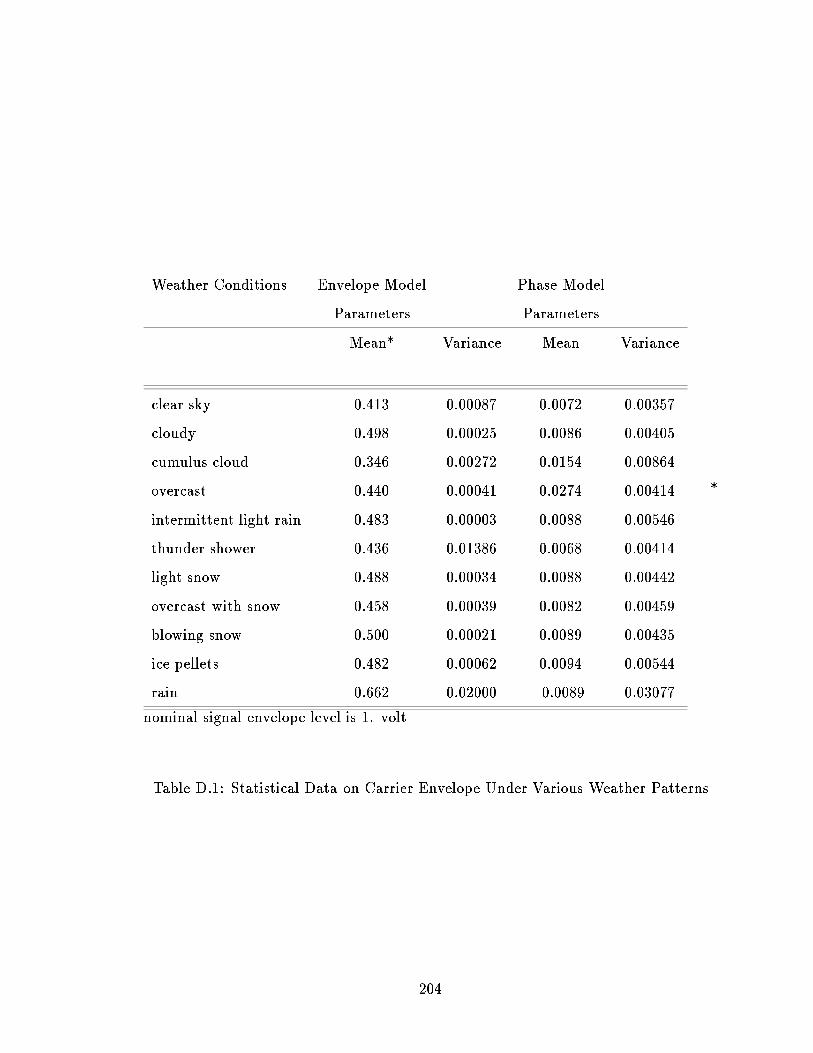
Weather Conditions Envelope Model Phase Model

Parameters Parameters

Mean* Variance Mean Variance

clear sky 0.413 0.00087 0.0072 0.00357

cloudy 0.498 0.00025 0.0086 0.00405

cumulus cloud 0.346 0.00272 0.0154 0.00864

overcast 0.440 0.00041 0.0274 0.00414

intermittent light rain 0.483 0.00003 0.0088 0.00546

thunder shower 0.436 0.01386 0.0068 0.00414

light snow 0.488 0.00034 0.0088 0.00442

overcast with snow 0.458 0.00039 0.0082 0.00459

blowing snow 0.500 0.00021 0.0089 0.00435

ice pellets 0.482 0.00062 0.0094 0.00544

rain 0.662 0.02000 -0.0089 0.03077

*

nominal signal envelope level is 1. volt

Table D.1: Statistical Data on Carrier Envelope Under Various Weather Patterns

204

on the weather conditions, while the energy of the sinusoid remains relatively constant

as indicated by the low variance of the envelope. Due to this low variance, the channel

will be modeled as a non-time varying system for the purposes of simulation. Other

models will be used to calculate the amount of attenuation of the signal.

D.2 Ionospheric Eects

The ionospheric eects are due to the charged particles in the atmosphere which result

from a number of sources, the most signicant of which is the solar wind. These

charged particles may cause attenuation and multipath eects that can degrade the

transmitted signal. An account of the ionospheric eects are presented below.

D.2.1 Refraction/Direction of Arrival Variation

The eects of refraction are not signicant for frequencies above 10 GHz. The beam-

forming algorithms used in the thesis are not dependent on knowing the direction

of arrival of the information. Average values for the direction of arrival variation

due to the ionosphere may be calculated in an actual design of a satellite system,

but this factor is considered unimportant for the purpose of simulating the eects of

beamforming on a satellite channel.

D.2.2 Faraday Rotation

Due to the anisotropy of the medium which results from the distribution of ionized

particles, linear polerized waves will suer an angular rotation according to the fol-

lowing formula

fd

=

2:36 10

4

f

2

B

av

Z

Ndl (D.1)

Where

205

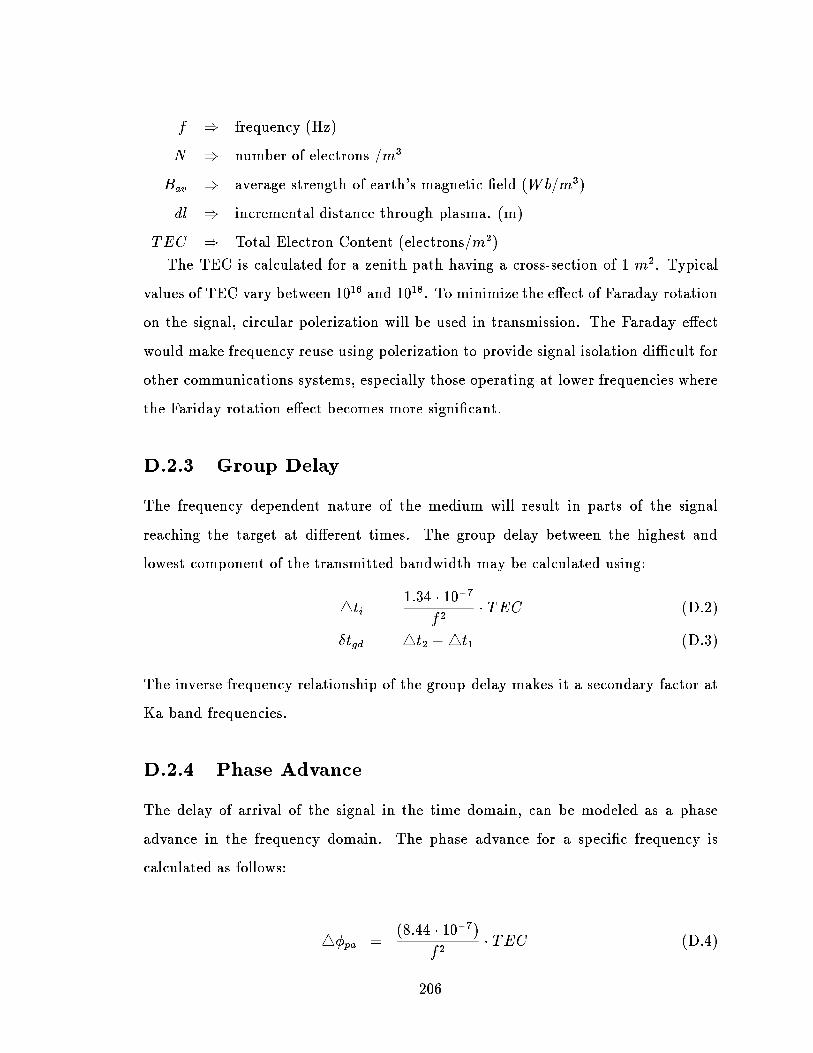
f ) frequency (Hz)

N ) number of electrons =m

3

B

av

) average strength of earth's magnetic eld (Wb=m

3

)

dl ) incremental distance through plasma. (m)

TEC ) Total Electron Content (electrons=m

2

)

The TEC is calculated for a zenith path having a cross-section of 1 m

2

. Typical

values of TEC vary between 10

16

and 10

18

. To minimize the eect of Faraday rotation

on the signal, circular polerization will be used in transmission. The Faraday eect

would make frequency reuse using polerization to provide signal isolation dicult for

other communications systems, especially those operating at lower frequencies where

the Fariday rotation eect becomes more signicant.

D.2.3 Group Delay

The frequency dependent nature of the medium will result in parts of the signal

reaching the target at dierent times. The group delay between the highest and

lowest component of the transmitted bandwidth may be calculated using:

4t

i

=

1:34 10

7

f

2

TEC (D.2)

t

gd

= 4t

2

4t

1

(D.3)

The inverse frequency relationship of the group delay makes it a secondary factor at

Ka band frequencies.

D.2.4 Phase Advance

The delay of arrival of the signal in the time domain, can be modeled as a phase

advance in the frequency domain. The phase advance for a specic frequency is

calculated as follows:

4

pa

=

(8:44 10

7

)

f

2

TEC (D.4)

206

d

pa

dt

=

(8:44 10

7

)

f

2

TEC (D.5)

The inverse relationship of the phase advance with respect to frequency makes

its impact on the overall signal a secondary eect. The phase advance phenomena

demonstrate a potential problem for broad band digital signals at lower frequencies

which would be aected by pulse smearing.

D.2.5 Doppler Frequency

The atmospheric conditions are time dependent in nature. Therefore the rate of

change of the phase advance results in a frequency uctuation. This may be calculated

as follows:

f

D

=

1:34 10

7

f

d(TEC)

dt

(D.6)

For the system studied in this thesis, the target station is assumed to be stationary

during transmission, therefore there is no Doppler shift due to the earth station unit.

The Doppler frequency with respect to the ionosphere is not considered signicant

at the Ka band frequency range due to the inverse frequency relationship. This

assumption is also supported by Loo's empirical statistical model presented in section

D.1.

D.2.6 Dispersion

The rate of change of the time delay with frequency is the dispersion of the signal

due to time delay. This quantity may be modeled as follows:

j 4

pd

j =

(8:44 10

7

)

f

2

B TEC (D.7)

The variable B is the bandwidth of the signal transmitted. the dispersion angle

is again an inverse function of frequency which makes the eect of dispersion on the

signal relatively small for the Ka band frequencies.

207

D.2.7 Ionospheric Scintillation

Ionospheric scintillation is caused by variations in the electron density. This will

cause a variation in focusing eect due to changes in Fresnel zones. The uctuations

are usually seen as a rapid variation in amplitude of the signal around a mean level.

For regions away from the geomagnetic equator, which have an elevation angle of

approximately 10 degrees or greater, and with a frequency above 10 GHz, the eects

of ionospheric scintillation are negligible.

D.2.8 Summary of Ionospheric Eects

Below is a table of the eects of ionospheric factors on a 20 GHz signal. These results

were scaled from data presented in [3]

Eect Frequency 20 GHz

Dependence

Faraday

1

f

2

0:28

Rotation

Propagation

1

f

2

0.625

delay ns

Refraction

1

f

2

< 0:09

00

Variation in

1

f

2

0:03

00

direction of of arc

arrival

Dispersion

1

f

2

0:5 10

7

ps/Hz

Table D.2: Calculation Summary of Ionospheric Eects

The high frequency eects of Ka band frequencies makes ionospheric eects on

the signal secondary as shown by the above table.

208

D.3 Clear Air Eects

Clear air eects primarily deal with the eects that the lower atmosphere has on

the radio signal. It has been presented in [3] that the most signicant in uence on

the magnitude of clear air interference comes from the elevation angle. For elevation

angles above 5 degrees, the eect of the atmosphere are usually only a secondary

consideration. The ray bending due to the troposphere is not considered relevant

for the channel model being developed in this thesis due to the blind beamforming

algorithms being considered.

D.4 Tropospheric Scattering

Tropospheric scattering is a result of turbulence in the lower earth atmosphere which

causes variations in the medium's density and composition. This becomes a signicant

for the signal when the elevation angle is below approximately 1 degree. Tropospheric

scattering was not modeled in this thesis.

D.5 Antenna Gain Reduction

The apparent reduction in the gain of an antenna increases as the eective aperture

increases. The eect of antenna gain reduction becomes larger as the frequency

increases. Allnutt [3] has presented a relation based on empirical data which gives

regions of antenna gain reduction based on the elevation angle and the beamwidth of

the re ector. The gain reduction is primarily a result of the phase distortion of the

received electric eld. This results in a nonuniform phase incident on the antenna

aperture. For a beamwidth of 0:2

, and an elevation angle of 20

, the antenna gain

is reduced by a factor of 0.5 dB. This gain reduction was incorporated in the link

budget analysis.

209

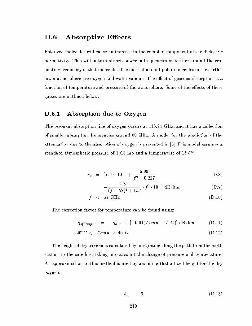
D.6 Absorptive Eects

Polerized molecules will cause an increase in the complex component of the dielectric

permutivity. This will in turn absorb power in frequencies which are around the res-

onating frequency of that molecule. The most abundant polar molecules in the earth's

lower atmosphere are oxygen and water vapour. The eect of gaseous absorption is a

function of temperature and pressure of the atmosphere. Some of the eects of these

gasses are outlined below.

D.6.1 Absorption due to Oxygen

The resonant absorption line of oxygen occurs at 118.74 GHz, and it has a collection

of smaller absorption frequencies around 60 GHz. A model for the prediction of the

attenuation due to the absorption of oxygen is presented in [3] This model assumes a

standard atmospheric pressure of 1013 mb and a temperature of 15 C

.

o

= [7:19 10

3

+

6:09

f

2

+ 0:227

(D.8)

+

4:81

(f 57)

2

+ 1:5

] f

2

10

3

dB/km (D.9)

f < 57 GHz (D.10)

The correction factor for temperature can be found using:

ojTemp

=

oj15

C

[0:01(Temp 15

C)] dB/km (D.11)

20

C < Temp < 40

C (D.12)

The height of dry oxygen is calculated by integrating along the path from the earth

station to the satellite, taking into account the change of pressure and temperature.

An approximation to this method is used by assuming that a xed height for the dry

oxygen.

h

o

= 6 (D.13)

210

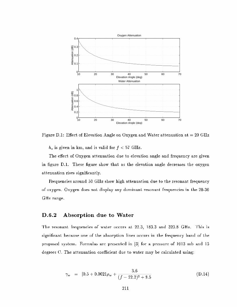
10 20 30 40 50 60 700

0.1

0.2

0.3

0.4Oxygen Attenuation

Elevation Angle (deg)

Atte

nuat

ion

(dB

)

10 20 30 40 50 60 700

0.2

0.4

0.6

0.8

1

Water Attenuation

Elevation Angle (deg)

Atte

nuat

ion

(dB

)

Figure D.1: Eect of Elevation Angle on Oxygen and Water attenuation at = 20 GHz

h

o

is given in km, and is valid for f < 57 GHz.

The eect of Oxygen attenuation due to elevation angle and frequency are given

in gure D.1. These gure show that as the elevation angle decreases the oxygen

attenuation rises signicantly.

Frequencies around 50 GHz show high attenuation due to the resonant frequency

of oxygen. Oxygen does not display any dominant resonant frequencies in the 20-30

GHz range.

D.6.2 Absorption due to Water

The resonant frequencies of water occurs at 22.3, 183.3 and 323.8 GHz. This is

signicant because one of the absorption lines occurs in the frequency band of the

proposed system. Formulas are presented in [3] for a pressure of 1013 mb and 15

degrees C. The attenuation coecient due to water may be calculated using:

w

= [0:5 + 0:0021

w

+

3:6

(f 22:2)

2

+ 8:5

(D.14)

211

0 50 100 150 200 250 300 35010

−2

10−1

100

101

102

103

Oxygen Attenuation

Frequency (GHz)

Atte

nuat

ion

(dB

)

0 50 100 150 200 250 300 35010

−2

10−1

100

101

102

103

Water Attenuation

Frequency (GHz)

Atte

nuat

ion

(dB

)

Figure D.2: Eect of Frequency on Oxygen and Water attenuation

+

10:6

(f 183:3)

2

+ 9:0

+

8:9

(f 325:4)

2

+ 26:3

]f

2

w

10

4

(D.15)

The correction factor for temperature can be found using:

wjTemp

=

wj15

C

[0:006(Temp 15

C)] dB/km (D.16)

20

C < Temp < 40

C (D.17)

This formula is accurate to within 15 % over the range of measured water vapour

density

w

of 0-50 g=m

3

.

The equivalent height for water vapour may be calculated by:

h

w

= h

wo

[1 +

3:0

(f 22:2)

2

+ 5

+

5:0

(f 183:3)

2

+ 6

+

2:5

(f 325:4)

2

+ 4

(D.18)

h

wo

has a value of 1.6 km in clear weather, and 2.1 km in rain. It is measured in

km and is valid for f < 350 GHz.

D.6.3 Total Gaseous Attenuation due to Absorption

The total zenith attenuation A

g

due to atmospheric gasses may be found as follows.

212

A

g

=

o

h

o

e

h

s

=h

o

+

w

hw

sin(

el

)

(D.19)

This formula is valid for slant angles

el

greater than 10 degrees, and f < 50 GHz.

The variable h

s

is the earth station's height above sea level.

D.7 Tropospheric Scintillation Eects

The eect of wind on the lower earth atmosphere tends to mix up the dierent

stratication layers of gas which causes a variations in the refractive index to occur

over small intervals at a rapid rates. Amplitude and phase variations due to the

change in the refractive index appear as amplitude variations at the receiving antenna.

Studies have shown [3] that the eect of the tropospheric scintillations increases with

frequency and with decreasing elevation angle.

The empirical data collected by Loo [27] shows that for a sinusoidal frequency

operating at the Ka frequency band, the variation in the signal amplitude is not

very large. The cyclostationary algorithms which will be employed depend only on

the preservation of the known carrier sinusoid, and should not be degraded by the

slight carrier envelope variations. (Section D.1). For this reason, the tropospheric

scintillation eects were not modeled in the channel. For a method on the modeling

of tropospheric scintillation refer to [3].

D.8 Attenuation Eects

The attenuation on the satellite signal is the most signicant eect in the link budget

analysis. The attenuation is a result of two main mechanisms which are absorption

and scattering.

The rst form of attenuation results when the medium absorbs some of the signal

energy. This energy is then retransmitted through thermal vibrations. The result

observed is an increase in the thermal noise of the system.

213

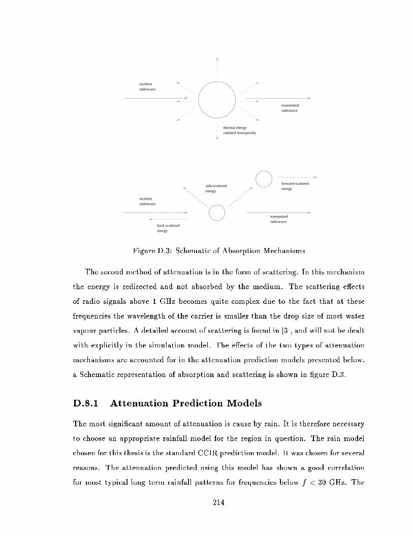
back-scattered energy

transmitted radiowave

transmitted radiowave

forward-scatteredenergy

side-scattered energy

incidentradiowave

incidentradiowave

thermal energy radiated isotropically

Figure D.3: Schematic of Absorption Mechanisms

The second method of attenuation is in the form of scattering. In this mechanism

the energy is redirected and not absorbed by the medium. The scattering eects

of radio signals above 1 GHz becomes quite complex due to the fact that at these

frequencies the wavelength of the carrier is smaller than the drop size of most water

vapour particles. A detailed account of scattering is found in [3], and will not be dealt

with explicitly in the simulation model. The eects of the two types of attenuation

mechanisms are accounted for in the attenuation prediction models presented below.

a Schematic representation of absorption and scattering is shown in gure D.3.

D.8.1 Attenuation Prediction Models

The most signicant amount of attenuation is cause by rain. It is therefore necessary

to choose an appropriate rainfall model for the region in question. The rain model

chosen for this thesis is the standard CCIR prediction model. It was chosen for several

reasons. The attenuation predicted using this model has shown a good correlation

for most typical long term rainfall patterns for frequencies below f < 30 GHz. The

214

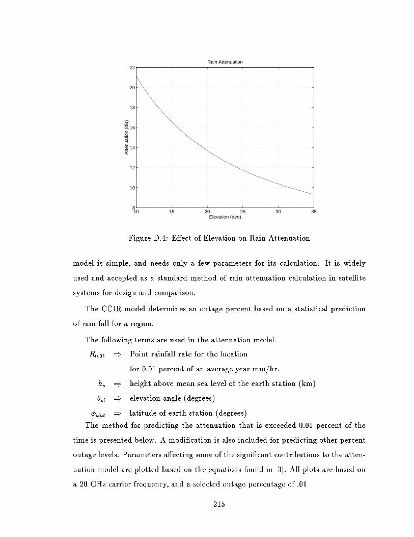
10 15 20 25 30 358

10

12

14

16

18

20

22Rain Attenuation

Elevation (deg)

Atte

nuat

ion

(dB

)

Figure D.4: Eect of Elevation on Rain Attenuation

model is simple, and needs only a few parameters for its calculation. It is widely

used and accepted as a standard method of rain attenuation calculation in satellite

systems for design and comparison.

The CCIR model determines an outage percent based on a statistical prediction

of rain fall for a region.

The following terms are used in the attenuation model.

R

0:01

) Point rainfall rate for the location

for 0.01 percent of an average year mm/hr.

h

s

) height above mean sea level of the earth station (km)

el

) elevation angle (degrees)

elat

) latitude of earth station (degrees)

The method for predicting the attenuation that is exceeded 0.01 percent of the

time is presented below. A modication is also included for predicting other percent

outage levels. Parameters aecting some of the signicant contributions to the atten-

uation model are plotted based on the equations found in [3]. All plots are based on

a 20 GHz carrier frequency, and a selected outage percentage of .01

215

17.5 18 18.5 19 19.5 20 20.5 21 21.5 22 22.510

0

101

102

Rain Attenuation

Frequency (GHz)

Atte

nuat

ion

(dB

)

27.5 28 28.5 29 29.5 30 30.5 31 31.5 32 32.510

1

102

Rain Attenuation

Frequency (GHz)

Atte

nuat

ion

(dB

)

Figure D.5: Eect of Frequency on Rain Attenuation

Figure D.4 shows that as the elevation angle decreases, the attenuation due to

rain increases signicantly. This behavior will aect the the selection of the target

location on the earth of the parabolic antenna.

Figure D.5 shows that as the frequency increases so does the attenuation due to

rain. It can be observed that the attenuation at 30 GHz is approximately 10 dB

higher than at 20 GHz. For this reason the downlink channel was chosen to be at 20

GHz due to the power limitations on the satellite.

The attenuation due to the height above sea level decreases with elevation as

shown in gure D.6. Locations closer to sea level receive more attenuation which is a

result of a thicker layer of precipitation.

The eect of the selected outage percent on the attenuation margin is also plotted.

This shows a steep rise in the attenuation margin for condence levels of greater than

0.01 % per year. Therefore the cost of decreasing the outage percent below 0.01 %

would be very expensive in terms of hardware or power.

The following collection of equations outline the calculation of the attenuation

parameters for the CCIR attenuation model as presented in [3]

216

0 0.1 0.2 0.3 0.4 0.5 0.6 0.7 0.8 0.9 17

7.5

8

8.5

9

9.5

10

10.5Rain Attenuation

Height (km)

Atte

nuat

ion

(dB

)

Figure D.6: Eect of Height Above Sea Level on Rain Attenuation

The rain height h

R

is calculated from the latitude of the station, and is in units

of km.

h

R

=

8

>

<

>

:

4:0 0<

el

< 36

4:0 0:075(

el

36)

el

> 36

(D.20)

The slant path for angles above

el

> 5

can be found using the following

equation. L

s

is calculated in km.

L

s

=

(h

R

h

s

)

sin(

el

)

(D.21)

The horizontal projection of the slant path is

L

G

= L

s

cos(

el

) (D.22)

The reduction factor r

0:01

for 0.01 % outage time can be calculated from

r

0:01

=

1

1 + 0:045L

G

(D.23)

217

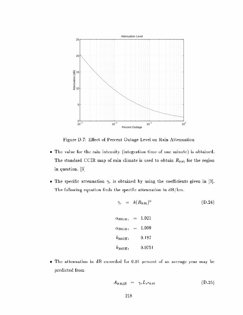
10−3

10−2

10−1

100

0

5

10

15

20

25Attenuation Level

Percent Outtage

Atte

nuat

ion

(dB

)

Figure D.7: Eect of Percent Outage Level on Rain Attenuation

The value for the rain intensity (integration time of one minute) is obtained.

The standard CCIR map of rain climate is used to obtain R

0:01

for the region

in question. [3]

The specic attenuation

r

is obtained by using the coecients given in [3].

The following equation nds the specic attenuation in dB/km.

r

= k(R

0:01

)

(D.24)

30GHz

= 1:021

20GHz

= 1:099

k

30GHz

= 0:187

k

20GHz

= 0:0751

The attenuation in dB exceeded for 0.01 percent of an average year may be

predicted from

A

0:01jR

=

r

L

s

r

0:01

(D.25)

218

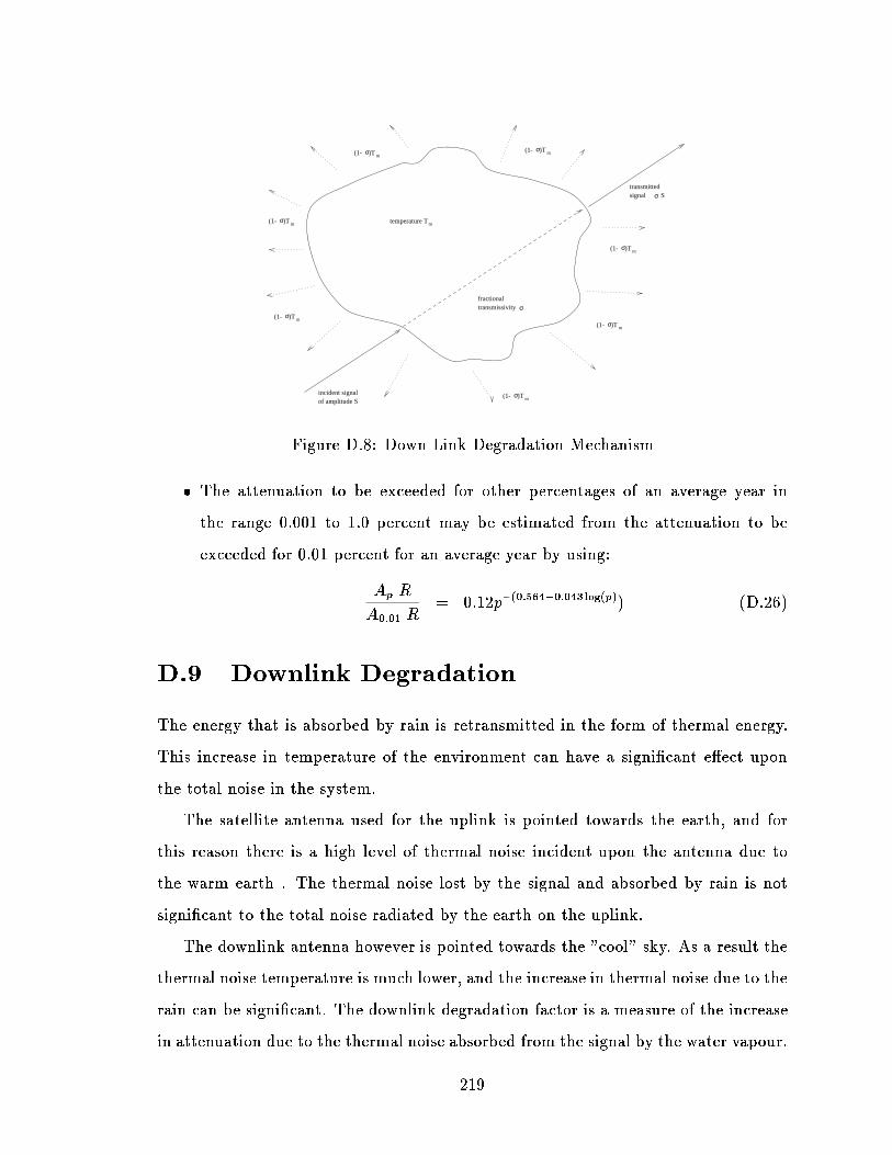
incident signalof amplitude S

fractional transmissivity σ

temperature Tm

transmitted signal Sσ

(1- )Tσm

(1- )Tσm

(1- )Tσm(1- )Tσ

m

(1- )Tσm

(1- )Tσm

(1- )Tσm

Figure D.8: Down Link Degradation Mechanism

The attenuation to be exceeded for other percentages of an average year in

the range 0.001 to 1.0 percent may be estimated from the attenuation to be

exceeded for 0.01 percent for an average year by using:

A

p

jR

A

0:01

jR

= 0:12p

(0:564+0:043log(p)

) (D.26)

D.9 Downlink Degradation

The energy that is absorbed by rain is retransmitted in the form of thermal energy.

This increase in temperature of the environment can have a signicant eect upon

the total noise in the system.

The satellite antenna used for the uplink is pointed towards the earth, and for

this reason there is a high level of thermal noise incident upon the antenna due to

the warm earth . The thermal noise lost by the signal and absorbed by rain is not

signicant to the total noise radiated by the earth on the uplink.

The downlink antenna however is pointed towards the "cool" sky. As a result the

thermal noise temperature is much lower, and the increase in thermal noise due to the

rain can be signicant. The downlink degradation factor is a measure of the increase

in attenuation due to the thermal noise absorbed from the signal by the water vapour.

219

Tf

antenna

T

feed run

T referenced to this point

receiver T

A

sys

r

σf

Figure D.9: Antenna Noise Schematic

Figure D.8 depicts schematically this mechanism.

To calculate the downlink degradation factor (DND), the following variables must

be dened. The variables are represented schematically on the diagram D.9

T

sys

) System noise temperature. (

K)

T

A

) Noise temperature incident on antenna. (

K)

T

r

) Receiver noise temperature (

K)

T

c

) Cosmic noise temperature (

K)

T

m

) Temperature of the medium (

K)

f

) Feed transmission factor

A

sky

) Total atmospheric attenuation (dB)

A

g

) Gaseous attenuation (dB)

A certain amount of the energy received by the antenna is absorbed by the feed

line to the receiver. The receiver in turn transmits some thermal noise which is

proportional to its temperature. The DND factor may be found using the following

steps.

220

The total system noise temperature must be found. This can be done using:

T

sys

= T

r

+ (1

f

)T

f

+

f

T

A

(D.27)

It is necessary to nd the clear sky attenuation with and without attenuation

due to rain.

T

Ajclearsky

= T

m

(1 10

A

g

=10

) + T

c

10

A

g

=10

) (D.28)

T

Ajrain

= T

m

(1 10

A=10

) + T

c

10

A=10

) (D.29)

A

g

may be calculated from equation D.19.

The downlink degradation factor is then calculated as follows:

DND = A+ 10 log(

T

sysjrain

T

sysjclearsky

) (D.30)

The DND can have a signicant aect on the level of received noise seen by the

earth station. For example, the following values were used:

A

g

=0.5 dB T

c

=2:7

K T

m

=280

K A=5.0 dB

f

= 0.95 T

f

=280

K T

r

=200

K

Here the resulting temperatures calculated were:

T

Ajclearsky

=39:2

K T

Ajrain

=192:3

K T

sysjclearsky

=245:3

K T

sysjrain

=396:7

K

From this the DND was found to be:

DND = 5 + 2:1 (D.31)

= 7:1 (D.32)

The additional increase of 2.1 dB in attenuation is signicant in the total link budget

calculation for system performance and capacity.

D.10 Frequency Scaling

The transmitted frequency band proposed is has a large bandwidth. For this reason

it was necessary to develop an accurate model that would frequency scale the atten-

uation at the band edges. This was signicant in determining if the signals on the

221

edge of the frequency channel would suer signicantly more or less than channels

closer to the target frequency. An empirical statistical model was used to achieve the

attenuation scaling parameters. The attenuation of a radio beacon at the frequencies

of 12.5, 20 and 30 GHz were measured over one year. Data was collected by a research

group in Blacksburg Virginia from the Olympus satellite at an elevation angle of 14

degrees. This angle provides a worst case scenario for coverage in Canada with a

geostationary satellite. The data in this experiment is unique due to the fact that

measurements were made simultaneously at all three frequencies. Using this data,

the following frequency scaling principle was derived based on the frequency scaling

power law. [25]

RAS

n

(f

L

; f

U

) =

ACA(f

U

)

ACA(f

L

)

(D.33)

= (

f

U

f

L

)

n

(D.34)

Where ACA is the attenuation due to clear sky conditions, and RAS is the statistical

attenuation ratio.

Analysis of the averaged data ratios for the factor n showed that the best value

to match the data when scaling from 20 to 30 GHz was 1.72. The average value for n

was found to be 1.9 for general frequency scaling across the Ka/Ku frequency bands.

This relation for the attenuation scaling is accurate 50 % of the time. For example,

if the attenuation at the lower frequency is exceeded 1 percent of the time per year,

then the frequency scaled result is exceeded 0.5 percent of the time. (50 percent of

one percent)

For a more accurate frequency scaling prediction, presented an empirical model

based on collected data. This model is accurate 99 percent of the time for attenuation

in the Ka/Ku band.

A(f

U

)

99%

= (

f

U

f

L

)

2:65

A(f

L

) 0:00138(

f

2

f

1

)

6:98

A(f

L

) (D.35)

222

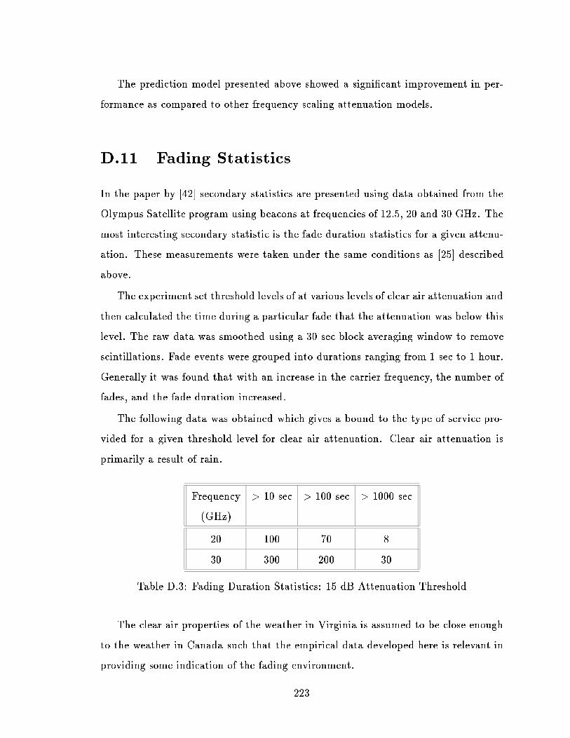
The prediction model presented above showed a signicant improvement in per-

formance as compared to other frequency scaling attenuation models.

D.11 Fading Statistics

In the paper by [42] secondary statistics are presented using data obtained from the

Olympus Satellite program using beacons at frequencies of 12.5, 20 and 30 GHz. The

most interesting secondary statistic is the fade duration statistics for a given attenu-

ation. These measurements were taken under the same conditions as [25] described

above.

The experiment set threshold levels of at various levels of clear air attenuation and

then calculated the time during a particular fade that the attenuation was below this

level. The raw data was smoothed using a 30 sec block averaging window to remove

scintillations. Fade events were grouped into durations ranging from 1 sec to 1 hour.

Generally it was found that with an increase in the carrier frequency, the number of

fades, and the fade duration increased.

The following data was obtained which gives a bound to the type of service pro-

vided for a given threshold level for clear air attenuation. Clear air attenuation is

primarily a result of rain.

Frequency > 10 sec > 100 sec > 1000 sec

(GHz)

20 100 70 8

30 300 200 30

Table D.3: Fading Duration Statistics: 15 dB Attenuation Threshold

The clear air properties of the weather in Virginia is assumed to be close enough

to the weather in Canada such that the empirical data developed here is relevant in

providing some indication of the fading environment.

223

Frequency > 10 sec > 100 sec > 1000 sec

(GHz)

20 70 30 10

30 200 100 30

Table D.4: Fading Duration Statistics: 20 dB Attenuation Threshold

224

The fading statistics give a measure of the type of performance that subscribers

to the system would have to deal with under worst case scenarios.

225

Appendix E

Coordinate System Transformations

Throughout this thesis it was necessary to use a variety of coordinate systems to

aid in calculations and for visualization of the physical geometry. This appendix

contains a summary of the coordinate systems used, under what conditions, and how

to transform among them.

The reference "Generation and Display of Satellite Antenna Patterns" by Cook et.

al. [8] provided the transformation formulas and the reference models needed.

E.1 Earth Centered System

The earth centered system is used in calculation of the beam foot prints and the

target position of the main beams. It is also used to output the maps corresponding

to the coverage location.

This coordinate system has its origin located at the center of the earth. The positive

z axis points to the north pole, the positive x axis intersects the Greenwich Meridian

and the positive y axis points 90

east according to the right hand rule. [8]

The following formulas are used to dene the spherical and Cartesian coordinates for

the earth centered system.

x

e

= R

e

cos(

e

) cos(

e

) (E.1)

y

e

= R

e

cos(

e

) sin(

e

) (E.2)

226

z

e

= R

e

sin(

e

) (E.3)

To transform from Cartesian to spherical coordinates:

R

e

= 6371km (E.4)

e

= sin

1

(z

e

=R

e

) (E.5)

e

= tan

1

(y

e

=x

e

) (E.6)

µ

ρ

e

e

R

z

x e

eGreenwich Meridian

Equator

Figure E.1: Earth Coordinate system Geometry

Here, the subscript "e" denotes the earth centered system, and the constant R

e

refers to the earth's radius. A geometric representation of the coordinate system is

shown in gure E.1.

227

E.2 Satellite Centered System

The satellite centered system has the z-axis pointing towards the center of the earth,

and the x-axis is oriented towards the north pole of the earth. The y-axis corresponds

to the orientation of a right handed coordinate system. Here the subscript "s" denotes

the satellite system. A geometric representation is shown in gure E.2.

x

y

z

Sub-Satellite Point

φ θ

T

s s

s

s

ss

Equator

View Window

Figure E.2: Satellite Coordinate system Geometry

x

s

= T

s

sin(

s

) cos(

s

) (E.7)

y

s

= T

s

sin(

s

) sin(

s

) (E.8)

z

s

= T

s

cos(

s

) (E.9)

E.3 Perspective Projection View of the Earth

There are a variety of ways of viewing a circular earth on a two dimensional surface.

The method that was chosen for this thesis was the perspective projection. The earth

228

is seen in perspective as viewed from a specic location in space. This method was

implemented using matlab's three dimensional graphics capabilities. The viewing

window is represented by the dotted box in gure E.2.

E.4 Coordinate Transform

In order to transform coordinates among the dierent reference system, the following

vectors were dened. A graphical representation of the system is depicted in gure

E.3.

xs

ys

s

r

t

x

zs

z

y

e

e

e

Figure E.3: Satellite Coordinate system Geometry

229

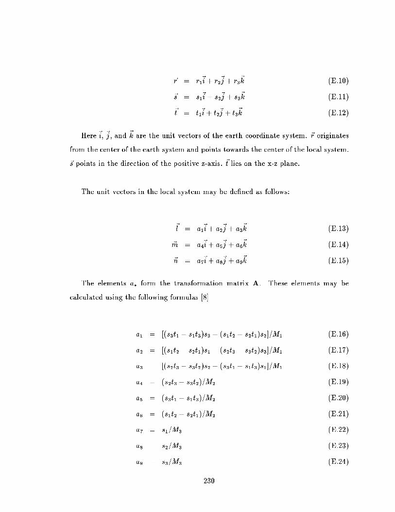
~r = r

1

~

i+ r

2

~

j + r

3

~

k (E.10)

~s = s

1

~

i+ s

2

~

j + s

3

~

k (E.11)

~

t = t

1

~

i+ t

2

~

j + t

3

~

k (E.12)

Here

~

i,

~

j, and

~

k are the unit vectors of the earth coordinate system. ~r originates

from the center of the earth system and points towards the center of the local system.

~s points in the direction of the positive z-axis.

~

t lies on the x-z plane.

The unit vectors in the local system may be dened as follows:

~

l = a

1

~

i+ a

2

~

j + a

3

~

k (E.13)

~m = a

4

~

i+ a

5

~

j + a

6

~

k (E.14)

~n = a

7

~

i+ a

8

~

j + a

9

~

k (E.15)

The elements a

form the transformation matrix A. These elements may be

calculated using the following formulas [8]

a

1

= [(s

3

t

1

s

1

t

3

)s

3

(s

1

t

2

s

2

t

1

)s

2

]=M

1

(E.16)

a

2

= [(s

1

t

2

s

2

t

1

)s

1

(s

2

t

3

s

3

t

2

)s

3

]=M

1

(E.17)

a

3

= [(s

2

t

3

s

3

t

2

)s

2

(s

3

t

1

s

1

t

3

)s

1

]=M

1

(E.18)

a

4

= (s

2

t

3

s

3

t

2

)=M

2

(E.19)

a

5

= (s

3

t

1

s

1

t

3

)=M

2

(E.20)

a

6

= (s

1

t

2

s

2

t

1

)=M

2

(E.21)

a

7

= s

1

=M

3

(E.22)

a

8

= s

2

=M

3

(E.23)

a

9

= s

3

=M

3

(E.24)

230

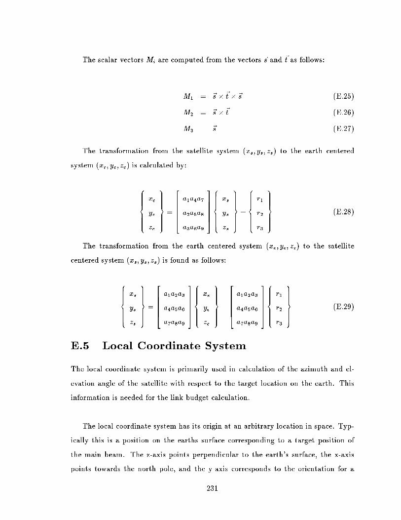
The scalar vectors M

i

are computed from the vectors ~s and

~

t as follows:

M

1

= ~s

~

t ~s (E.25)

M

2

= ~s

~

t (E.26)

M

3

= ~s (E.27)

The transformation from the satellite system (x

s

; y

s

; z

s

) to the earth centered

system (x

e

; y

e

; z

e

) is calculated by:

8

>

>

>

>

>

<

>

>

>

>

>

:

x

e

y

e

z

e

9

>

>

>

>

>

=

>

>

>

>

>

;

=

2

6

6

6

6

6

4

a

1

a

4

a

7

a

2

a

5

a

8

a

3

a

6

a

9

3

7

7

7

7

7

5

8

>

>

>

>

>

<

>

>

>

>

>

:

x

s

y

s

z

s

9

>

>

>

>

>

=

>

>

>

>

>

;

+

8

>

>

>

>

>

<

>

>

>

>

>

:

r

1

r

2

r

3

9

>

>

>

>

>

=

>

>

>

>

>

;

(E.28)

The transformation from the earth centered system (x

e

; y

e

; z

e

) to the satellite

centered system (x

s

; y

s

; z

s

) is found as follows:

8

>

>

>

>

>

<

>

>

>

>

>

:

x

s

y

s

z

s

9

>

>

>

>

>

=

>

>

>

>

>

;

=

2

6

6

6

6

6

4

a

1

a

2

a

3

a

4

a

5

a

6

a

7

a

8

a

9

3

7

7

7

7

7

5

8

>

>

>

>

>

<

>

>

>

>

>

:

x

e

y

e

z

e

9

>

>

>

>

>

=

>

>

>

>

>

;

2

6

6

6

6

6

4

a

1

a

2

a

3

a

4

a

5

a

6

a

7

a

8

a

9

3

7

7

7

7

7

5

8

>

>

>

>

>

<

>

>

>

>

>

:

r

1

r

2

r

3

9

>

>

>

>

>

=

>

>

>

>

>

;

(E.29)

E.5 Local Coordinate System

The local coordinate system is primarily used in calculation of the azimuth and el-

evation angle of the satellite with respect to the target location on the earth. This

information is needed for the link budget calculation.

The local coordinate system has its origin at an arbitrary location in space. Typ-

ically this is a position on the earths surface corresponding to a target position of

the main beam. The z-axis points perpendicular to the earth's surface, the x-axis

points towards the north pole, and the y-axis corresponds to the orientation for a

231

y

z

x

To Satellite

L

L

L

ε

−α

yL

xL

zL

y

z

x

e

e

e

es

es

Figure E.4: Local Coordinate system Geometry

232

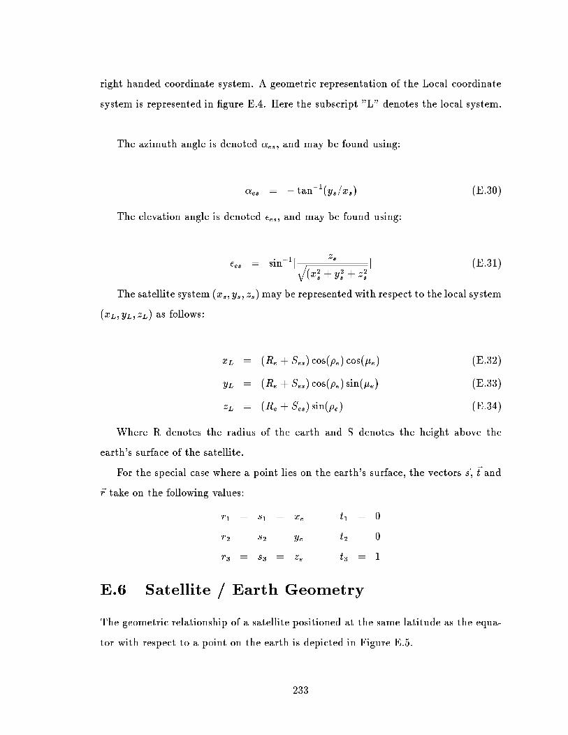
right handed coordinate system. A geometric representation of the Local coordinate

system is represented in gure E.4. Here the subscript "L" denotes the local system.

The azimuth angle is denoted

es

, and may be found using:

es

= tan

1

(y

s

=x

s

) (E.30)

The elevation angle is denoted

es

, and may be found using:

es

= sin

1

[

z

s

q

(x

2

s

+ y

2

s

+ z

2

s

] (E.31)

The satellite system (x

s

; y

s

; z

s

) may be represented with respect to the local system

(x

L

; y

L

; z

L

) as follows:

x

L

= (R

e

+ S

es

) cos(

e

) cos(

e

) (E.32)

y

L

= (R

e

+ S

es

) cos(

e

) sin(

e

) (E.33)

z

L

= (R

e

+ S

es

) sin(

e

) (E.34)

Where R denotes the radius of the earth and S denotes the height above the

earth's surface of the satellite.

For the special case where a point lies on the earth's surface, the vectors ~s,

~

t and

~r take on the following values:

r

1

= s

1

= x

e

r

2

= s

2

= y

e

r

3

= s

3

= z

e

t

1

= 0

t

2

= 0

t

3

= 1

E.6 Satellite / Earth Geometry

The geometric relationship of a satellite positioned at the same latitude as the equa-

tor with respect to a point on the earth is depicted in Figure E.5.

233

ze

θ

ε

ε

S

T

es

es

s

s

Figure E.5: Satellite-Earth Geometric relationship

234

The target position of a beam on the earth may be represented by the variables

(T

es

;

s

;

s

) which are shown in the gure E.5.

T

es

= (S

es

+R

e

) cos(

s

)

q

R

2

(S

es

+R

e

)

2

sin

2

(

s

) (E.35)

R

e

cos(

es

) = (S +R) sin(

s

) (E.36)

R

e

sin(

es

) =

q

R

2

e

(S

es

+R

e

)

2

sin

2

(

s

) (E.37)

235

Appendix F

Calculation of Satellite Feed Coordinates

The following method was developed to nd the coordinates of the satellite feed

positions which correspond to dierent target locations on the earth. Figure F.1

shows the physical modeling of the problem. The satellite must be positioned at

0 degrees latitude to maintain a geostationary orbit. The longitude position of the

satellite is stationed in the center of the coverage area.

ya

ys

xa

xs

za

zs

target

τ

reference satellite point

satellite point

sub-satellite point

equator

a

Figure F.1: Earth-Satellite Target Geometry

The antenna is aimed at a point on the earth which is ideally in the center of the

coverage area. This point on the earth corresponds to the on focus feed position, and

is dened as the reference target location or reference beam. This beam lies parallel

to the z axis of the antenna coordinate system which is used to calculate the feed

locations for the other target beams.

All coordinates are transformed into the satellite antenna reference system. The

236

ya ys

za

xa

xs

zs

saτ

xr

xazr

ya

yr

za

Feed Plane

Reflector Surface

τ

Feed Plane

Satellite Coordinates

AntennaCoordinates

Parent Reflectorr Surface

Offset Reflector Surface

On Focus Beam

rθ

Ω

α

a

a

Figure F.2: Antenna Feedplane Geometry, Y-Plane

237

angle

sa

species the angle the antenna axis makes with the satellite system in the xz

plane. There is no oset angle in the zy plane because the satellite and the antenna

are located directly above the target on the earth in the longitudinal coordinate. See

F.2 for a detail of the geometry. The incoming angle of a target beam is broken up

into two components, the xz component and the yz component.

The re ected angle in the yz component can be found using simple angle of inci-

dence equals the angle of re ection principle. This angle is specied by

r

All feeds

are assumed to be aimed towards the geometric center of the oset parabola.

xa

ya za

Feed Plane

Centered Beam

Offset Beam

Feed Location for Offset Beam

α

Ωγ

len

a

y

x

z

ar

ra

ra

ra

Figure F.3: Antenna Feed Plane Geometry, XZ-Plane

The re ected angle in the xz plane is depicted in gure F.3 This angle can be

calculated as follows:

a

is calculated for the system by dividing the known angle

a

by two.

a

was

238

found in the calculation of the re ector geometry.

a

=

a

=2 (F.1)

The re ected angle is therefore the negative of the incident angle and the line

parallel to z

a

. Here the subscript ta refers to the target's Cartesian coordinates

in the antenna reference system.

r

= (tan

1

(x

ta

=z

ta

) + 2

a

) BDF (F.2)

The coordinates of the re ector center is calculated with respect to the antenna

coordinate position. Since the satellite is positioned above the reference beam

location in longitude, the coordinates may be found using:

x

ra

= len sin(

a

) (F.3)

y

ra

= 0 (F.4)

z

ra

= len cos(

a

) (F.5)

~

V

r

= (x

ra

; y

ra

; z

ra

) (F.6)

The normal of the feed plane is found with respect to the antenna coordinate

system as follows:

x

nf

= sin(

a

) (F.7)

y

nf

= 0 (F.8)

z

nf

= cos(

a

) (F.9)

~

N

f

= (x

nf

; y

nf

; z

nf

) (F.10)

A direction vector for each target location from the oset re ector's center to

the feed plane is calculated. The constant M

d

is the magnitude of the direction

vector, and is used to normalize the cartesian coordinates.

x

da

= sin(

r

) (F.11)

239

y

da

= sin(

r

) (F.12)

z

da

= cos(

r

) (F.13)

M

d

=

q

x

2

da

+ y

2

da

+ z

2

da

(F.14)

~

V

d

= (x

da

; y

da

; z

da

)=M

d

(F.15)

A parametric method is used to calculate the intersection of each direction

vector with the feed plane. [4]

t

feed

=

~

N

f

~

V

r

~

V

d

~

N

f

(F.16)

The parameter t

feed

is used to calculate the length of the direction vector nec-

essary for the intersection with the feed plane.

x

f

= x

ra

+ x

da

t (F.17)

y

f

= y

ra

+ y

da

t (F.18)

z

f

= z

ra

+ z

da

t (F.19)

~

V

f

= (x

f

; y

f

; z

f

) (F.20)

xf

yf

ya

xa

za

yf

xf

εΓfeed

feed

Figure F.4: Geometry of Polar Coordinate Transform

The z

f

component for the intersection always resulted in a zero value.

The points of intersection are transformed into polar coordinates on the feed

plane. The geometry of this transform is depicted in gure F.4.

feed

=

q

x

2

f

+ y

2

f

(F.21)

feed

= tan

1

(y

f

=x

f

) (F.22)

240

Bibliography

[1] B.G. Agee. The property restoral approach to blind adaptive signal extraction.

PhD thesis, University of California, 1989.

[2] B.G. Agee, S.V. Schell, and W.A. Gardner. Spectral Self-Coherence Restoral:

A New Approach to Blind Adaptive Signal Extraction Using Antenna Arrays.

IEEE Proceedings, 4:753 766, April 1990.

[3] J.E. Allnutt. Satellite to ground radiowave propagation. Peter Peregrinus Ltd.,

1989.

[4] H. Anton. Elementary Linear Algebra. John Wiely and Sons, 4 edition, 1984.

[5] T.E. Biedka. Subspace-constrained SCORE algorithms. In Proceedings of the

Asilomar Conference on Signals, Systems and Computers, pages 716 720,

November 1993.

[6] E. Bodewig. Matrix Calculus. North Holland Publishing Company, Amsterdam,

Holland, 1956.

[7] L. Castedo, A.R. Figueiras-Vidal, C.Y Tseng, and L.J Griths. Linearly con-

strained adaptive beamforming using cyclostationary signal properties. In IEEE

International Conference on Acoustics, Speech and Signal Processing, volume IV,

pages 249 252, 1994.

[8] W.L. Cook, D.D Opiedun, and L.R. Karl. Generation and Display of Satellite

Antenna Patterns. Comsat Technical Review, 19(2):259297, 1989.

241

[9] J. Cui, D.D. Falconer, and A.U.H. Sheikh. A phase algorithm for blind adaptive

optimum diversity combining. In Vehicular Technology Conference Proceedings,

June 1995.

[10] E.C. DuFort. Optimum Low Sidelobe High Crossover Multiple Beam Antennas.

IEEE Transactions on Antennas and Propagation, 33(9):946 954, 1985.

[11] J. Duggan. Parabolic Antenna Beamforming. Master's thesis, Queen's Univer-

sity, 1996.

[12] R.S. Elliott. Antenna THeory and Design. Prentice-Hall, 1981.

[13] R.J Fang. Lecture Notes in Control and Information Sciences 182: Advanced

Methods for Satellites and Deep Space Communications. COMSAT Corporation,

1992.

[14] W.A. Gardner. Representation and Estimation of Cyclostationar Processes. PhD

thesis, University of Massachusetts, Amherst, MA, 1972.

[15] W.A. Gardner. Spectral correlation of modulated signals: Part I - Analogue

modulation. IEEE Transactions on Communications, 35:584 594, June 1987.

[16] W.A. Gardner. Statistical Spectral Analysis: A Non-Probabilistic Theory.

Prentice-Hall, Englewood Clifs, NJ, 1987.

[17] W.A. Gardner. Cyclic Wiener lterint: theory and method. IEEE Transactions

on Communications, 41:151 163, January 1993.

[18] S. Grossman. Calculus. Academic Press Inc., 3 edition, 1984.

[19] S. Haykin. An Introduction to Analog and Digital Communications. John Wiley

& Sons, Toronto, 1989.

[20] K. Hirasawa. Analysis, design and measurement of small and low-prole anten-

nas. Artech House, 1992.

242

[21] J. Karimi. Personal Han-Held Communications Via L-Band CDMA-Based Geo-

stationary Beamforming Satellites. Master's thesis, Queen's University, 1996.

[22] J.D. Kraus. Antennas. McGraw-Hill, 1988.

[23] H. Lam. Analogue and Digital Filter Design: Design and Realization. Prentice-

Hall Inc., 1979.

[24] P. Lam, S. Lee, C. Donald, Chang, and Lang. Directivity Optimization of a

Re ector Antenna with Cluster Feeds: A Closed-Form Solution. IEEE Transac-

tions on Antennas and Propagtion, 33(11):1163 1473, 1985.

[25] J.D. Laster and L.S. Warren. Frequency Scaling of Rain Attenuation for Satel-

lite Communication Links. IEEE Transactions on Antennas and Propagation,

43(11):1207 1216, 1995.

[26] S.W. Lee and Y. Rahmat-Samii. Simple Formulas for Designing an Oset Multi-

beam Parabolic Re ector. IEEE Transactions on Antennas and Propagation,

29(3):472478, 1981.

[27] C. Loo. Statistic Models for Land Mobile and Fixed Satellite Communications

at Ka Band. In IEEE Vehicular Technology Conference, 1996.

[28] R.A. Monzingo and T.W. Miller. Introduction to Adaptive Arrays. Wiley, New

York, 1980.

[29] A. Papoulis. Probability, Random Variables, and Stochastic Processes. Mc Graw

Hill, 2 edition, 1989.

[30] R.A. Pearson, Y. Kalatidazeh, B.G. Driscoll, G.T. Philippou, B. Claydon, and

D.J Brain. Application of Contoured Beam Shaped Re ector Antannas to Mis-

sion Requirements. In IEE 8th International Confrence on Antennas and Prop-

agation, pages 9 13, United Kingdom, March 1993.

243

[31] C.J. Pike. EHF(28/19 GHz) Suitcase Satellite Terminal. In Proceedings of the

Olympus Utilisation Conference, pages 203 207, Sevilla, Spain, April 1993.

[32] J.G. Proakis. Digital Communicaions. Mc Graw-Hill, Montreal, 1989.

[33] K.S. Rao, G.A. Morin, M.Q. Tang, and S. Richard. Development of a 45 GHz

Multiple Beam Antenna for Millitary Satellite Communications. IEEE Transac-

tions on Antennas and Propagation, 43(10):1036 1046, 1995.

[34] M.E. Rollins and C Loo. Cyclic Beamforming Algorithms for Future Broad-band

Satellite Communications Systems Employing On-Board Processing. Technical

report, Communications Research Center, Ottawa, December 1995.

[35] S.V. Schell and B.G. Agee. Application of the SCORE alogrithm and SCORE

extensions to sorting in the rank-L spectral selfcoherence environment. In Pro-

ceedings of the 22nd Asilomar Conference on Signals, Systems and Computers,

pages 274 278, 1988.

[36] R.O. Schmidt. A Signal Subspace Approach to Multiple Emitter Location and

Spectral Estimation. PhD thesis, Stanford University, November 1981.

[37] J. Shynk and R. Gooch. The Constant Modulus Array for Cochannel Signal

Copy and Direction Finding. IEEE Transactions on Signal Processing, 44(3):652

660, March 1996.

[38] K.P. Spy and E.J. Haakinson. Calculation of Geostationary Satellite Footprints

for Certain Idealized Antennas. U.S. Department of Commerce, October 1980.

[39] S. Stein. On cross coupling in multiple-beam antennas. IRE Transactions on

Antennas and Propagation, 10:548, 1962.

[40] W. Tranter and R. Ziemer. Principles of Communications. John Wiley and

Sons, 4 edition, 1995.

244

[41] B. Van Veen and K.M. Buckley. Beamforming: A versitile approach to spatial

ltering. IEEE ASSP Magazine, pages 4 23, April 1988.

[42] L.S. Warren, T. Pratt, A. Safaai-Jazi, P.W Remaklus, J. Laster, B. Nelson,

and H. Ajaz. Results for the Virginia Tech Propagation Experiment Using the

Olympus Satellite 12, 20 and 30 GHz Beacons. IEEE Transactions on Antennas

and Propagation, 43(1):54 62, 1995.

[43] T.R. Watereld. Design Features of the Orion Satellite Antenna Subsystem. In

IEE 8th International Confrence on Antennas and Propagation, pages 95 98,

United Kingdom, March 1993.

[44] J.H Winters. Optimum combining in digital mobile radio with cochannel inter-

ference. IEEE journal on Selected Areas in Communications, 2(4):528 539,

July 1984.

[45] Q Wu. Fast algorithm for adaptive beamforming of cyclic signals. IEE Proceed-

ings on Radar, Sonar and Navigation, 141(6):312 318, December 1994.

[46] Q. Wu and K.M. Wong. Adaptive beamforming of cyclic signal and fast imple-

mentation. In IEEE International Conference on Acoustics, Speech and Signal

Processing, volume IV, pages 157 160, 1994.

[47] A.R. Zieger, D.W. Hancock, G.S. Hayne, and C.L. Purdy. NASA Radar Altime-

ter for the TOPEX/Poesidon Project. Proceedings of the IEEE, 79(6):810 826,

1991.

245

Vita

Paul James Lusina

EDUCATION

M.Sc (19951997), Electrical & Computer Engineering, Queen's University

B.Sc. (19901995), Engineering Science: Electrical Option, University of Toronto

International Baccalaureate Diploma (19881990), Victoria Park Secondary School

LANGUAGES

Two Ontario Academic Credits in French and three summer work terms in French

speaking communities.

One year of introductory German in preparation for the

Ontario/Baden-Wurttemberg exchange program at the University of Ulm. (97-98)

EXPERIENCE

Queen's University, Kingston, Ontario (Sept 95 Present)

Teaching Assistant (Image Processing & Communications Lab)

Teleste Antenni Oy, Littionen Finland (May/95 Aug/95)

Design Engineer

246

Northern Telecom: Product Assurance Component Evaluation Lab.

Ottawa, Ontario (May/93 Aug/94)

Test Engineer

General Comminution Inc, Toronto, Ontario (May/92 Aug/92)

Test Technician

Ministere Des Telecommunications, Ste. Foy, Quebec (May/91 Aug/91)

Research Technician

PUBLICATIONS

Lusina, Karimi, Blostein, "Broadband Satellite Coverage of Canada Using Parabolic

Antennas and Beamforming", Proceedings for the CITR Conference, pp83-84. August

1996, Montebello, Quebec, Canada.

247

Abstract - Queen's Universitypost.queensu.ca/~sdb2/PAPERS/thesis_lusina.pdf · Link Budget...

Documents

Transcript of Abstract - Queen's Universitypost.queensu.ca/~sdb2/PAPERS/thesis_lusina.pdf · Link Budget...