Abstract Cryogenic Optomechanics with a Silicon Nitride Membrane

Mitchell James Underwood III 2016

The field of optomechanics involves the study of the interaction between light and matter via

the radiation pressure force. Though the radiation pressure force is quite weak compared with forces

we normally experience in the macroscopic world, modern optical and microwave resonators are able to

enhance the radiation pressure force so that it can be used to both measure and control the motion of

macroscopic mechanical oscillators. Recently, optomechanical systems have reached a regime where

the sensitivity to mechanical motion is limited only by quantum effects. Together with optical cooling

techniques such as sideband cooling, this sensitivity has allowed experiments to probe the quantum

behaviors of macroscopic objects, and also the quantum limits of measurement itself. In this dissertation

I describe the physics underlying the modern field of optomechanics and provide an overview of

experimental accomplishments of the field such as ground state cooling of mechanical oscillators,

detection of radiation pressure shot noise, and preparation, storage, and transfer of quantum states

between macroscopic objects and the electromagnetic field. I then describe the specific experimental

work done in pursuit of my degree involving the ground state cooling of a silicon nitride membrane in a

high finesse Fabry-Perot cavity, and a systematic characterization of the dynamics that occur when the

membrane is coupled to two nearly degenerate cavity modes at an avoided crossing in the cavity

spectrum. In the section on ground state cooling, particular attention is given to the influence of

classical laser noise on the measurement of the membrane’s motion at low phonon occupancies, and

techniques for laser noise measurement and reduction are discussed.

1

Cryogenic Optomechanics with a Silicon Nitride Membrane

A Dissertation Presented to the Faculty of the Graduate School of

Yale University in Candidacy for the Degree of

Doctor of Philosophy

by Mitchell James Underwood III

Dissertation Director: Jack Harris

December 2016

2

© 2016 by Mitchell James Underwood III All Rights Reserved.

3

Acknowledgements

There are many people I would like to thank for supporting me throughout the course of my

research. First, of course, is Jack Harris for being an excellent mentor and providing me with the

opportunity to work on such an exciting project. Next, are Donghun Lee and David Mason, my

colleagues who worked with me throughout the entirety of the experiments described in this

dissertation, helping to make them a success. There are also Haitan Xu, and Luyao Jiang, who joined the

group just as the research in this dissertation was wrapping up, but who nonetheless made valuable

contributions. Frequent conversations with Alexey Shkarin, Anna Kashkanova, Nathan Flowers-Jacobs,

and Scott Hoch were also much appreciated. I’d also like to thank Jack Sankey, Andrew Jayich, and Brian

Yang for their work on version 1.0 of the ground state cooling experiment, which gave us an idea of

where to start the research described here.

On a more personal level, I would like to thank Ashley Watts for her daily support throughout

graduate school, and my parents Mitchell and Susan Underwood for raising me to be the scholar I have

become.

Finally, I would like to thank Nufern, Inc. (my current employer), and my supervisor Peyman

Ahmadi, for their flexibility as I finished up this dissertation and moved on to my career.

4

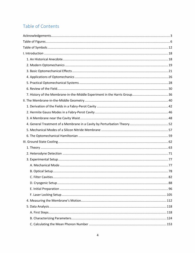
Table of Contents Acknowledgements ....................................................................................................................................... 3

Table of Figures ............................................................................................................................................. 6

Table of Symbols ......................................................................................................................................... 12

I. Introduction ............................................................................................................................................. 18

1. An Historical Anecdote........................................................................................................................ 18

2. Modern Optomechanics ..................................................................................................................... 19

3. Basic Optomechanical Effects ............................................................................................................. 21

4. Applications of Optomechanics .......................................................................................................... 26

5. Practical Optomechanical Systems ..................................................................................................... 28

6. Review of the Field .............................................................................................................................. 30

7. History of the Membrane-in-the-Middle Experiment in the Harris Group......................................... 36

II. The Membrane-in-the-Middle Geometry ............................................................................................... 40

1. Derivation of the Fields in a Fabry-Perot Cavity ................................................................................. 42

2. Hermite Gauss Modes in a Fabry-Perot Cavity ................................................................................... 46

3. A Membrane near the Cavity Waist .................................................................................................... 48

4. General Treatment of a Membrane in a Cavity by Perturbation Theory ............................................ 52

5. Mechanical Modes of a Silicon Nitride Membrane ............................................................................ 57

6. The Optomechanical Hamiltonian ...................................................................................................... 59

III. Ground State Cooling ............................................................................................................................. 62

1. Theory ................................................................................................................................................. 63

2. Heterodyne Detection ........................................................................................................................ 71

3. Experimental Setup ............................................................................................................................. 77

A. Mechanical Mode ........................................................................................................................... 77

B. Optical Setup ................................................................................................................................... 78

C. Filter Cavities ................................................................................................................................... 82

D. Cryogenic Setup .............................................................................................................................. 88

E. Initial Preparation ........................................................................................................................... 96

F. Laser Locking Setup ....................................................................................................................... 105

4. Measuring the Membrane’s Motion ................................................................................................. 112

5. Data Analysis ..................................................................................................................................... 118

A. First Steps...................................................................................................................................... 118

B. Characterizing Parameters ............................................................................................................ 124

C. Calculating the Mean Phonon Number ........................................................................................ 153

5

6. Future Directions .............................................................................................................................. 161

IV. Quadratic Optomechanics ................................................................................................................... 164

1. Introduction to Avoided Crossings .................................................................................................... 165

2. Theory ............................................................................................................................................... 171

3. Experimental Setup ........................................................................................................................... 178

A. Mechanical Mode ......................................................................................................................... 179

B. Optical Setup, Locking, and Measurement ................................................................................... 179

C. Characterizing Parameters ............................................................................................................ 184

4. Results ............................................................................................................................................... 189

5. Future Directions .............................................................................................................................. 202

V. Conclusion ............................................................................................................................................. 205

VI. Works Cited.......................................................................................................................................... 207

6

Table of Figures

Figure 1: Photophone transmitter (left) 2, and receiver (right) 3 ................................................................. 19

Figure 2: Schematic of the canonical optomechanical system. .................................................................. 21

Figure 3: Spectrum of light exiting the optical cavity after the interaction of an on-resonance optical drive with the moveable mirror. .................................................................................................... 22

Figure 4: Spectrum of light exiting the optical cavity after the interaction of a red detuned (left) or blue detuned (right) optical drive with the moveable mirror. .............................................................. 23

Figure 5: Illustration of Branginskiĭ, Manukin, and Tikhonov’s microwave cavity with moveable wall.. ... 31

Figure 6: Top, illustration of a membrane in the middle of a Fabry-Perot optical cavity, with the intracavity field plotted in red. Bottom, plot of the cavity detuning as a function of membrane position. ......................................................................................................................................... 41

Figure 7: Transverse spatial mode profiles of the first 9 Hermite Gauss optical cavity modes. ................ 46

Figure 8: Schematic of a partially reflective membrane inside an optical cavity. ...................................... 48

Figure 9: Numerically generated plot of cavity resonant frequency in units of free spectral range vs. membrane position normalized to wavelength. ........................................................................... 52

Figure 10: A plot of the result of numerical integration of Equation (36) with parameters selected to match those used in the experiment. ............................................................................................ 55

Figure 11: A plot of the frequencies of the (0,0), (0,2), (1,1), and (2,0) transverse modes of the optical cavity for a membrane of thickness 𝑡 = 50 nm and a membrane tilt of ~0.29° along both the x and y axes....................................................................................................................................... 56

Figure 12: Scanning electron micrograph of a membrane similar to the ones used in the experiments. . 58

Figure 13: 3D plots of the first nine mechanical modes of a square membrane. ...................................... 59

Figure 14: Schematic representation of contributions to the red (left) and blue (right) sidebands for a membrane with phonon number 𝑛𝑚 = 0 ..................................................................................... 76

Figure 15: 3D plot of the (2, 2) vibrational mode of the membrane, with phase selected such that antinodes are at their maximum deviations from equilibrium. .................................................... 78

Figure 16: Schematic of the optical setup for the ground state cooling experiment. ................................ 79

Figure 17: Combined spectrum of the lasers showing their detunings relative to the cavity resonances. 81

7

Figure 18: Spectrum of the photocurrent produced when the lasers land on the PDA10CF photodiode. 82

Figure 19: Photograph of filter cavity FC2. ................................................................................................. 84

Figure 20: CAD drawing showing the filter cavity sitting on its kinematic mount. ..................................... 85

Figure 21: Photograph of the complete optical setup of FC2. .................................................................... 87

Figure 22: CAD drawing of the cryogenic stage. See main text for a thorough description....................... 89

Figure 23: Photograph of the cryogenic stage. ........................................................................................... 92

Figure 24: A top down photograph of the cryostat during assembly of the vibration isolation system. ... 93

Figure 25: Photograph of a prototype of the membrane mounting assembly. ......................................... 95

Figure 26: Photograph of the membrane assembly resting inside the cryogenic optical cavity. ............... 96

Figure 27: Photograph of the alignment setup. .......................................................................................... 97

Figure 28: Schematic of the initial alignment setup. .................................................................................. 98

Figure 29: Plot of 935 nm light transmission measured by the germanium photodiode as a function of linear displacement of one of the collimator PiezoKnobs. .......................................................... 101

Figure 30: A plot of the cavity reflection as a function of membrane position and laser frequency, informally called a “bandstructure”. ........................................................................................... 104

Figure 31: Block diagram of electrical circuit for locking the measurement laser to the optical cavity. . 106

Figure 32: Schematic of the electrical circuit used to lock the cooling laser to the measurement laser with an adjustable frequency offset. ........................................................................................... 109

Figure 33: Plot of the frequency difference between the measurement and cooling laser optical modes as a function of membrane position. ........................................................................................... 110

Figure 34: Schematic of the filter cavity locking circuits. ......................................................................... 111

Figure 35: Electrical schematic of the circuit used to isolate and digitize the heterodyne signal from the photocurrent. ............................................................................................................................... 113

Figure 36: Left: A demodulated time trace of the red sideband of the membrane’s motion at 10 µW cooling power. Right: A zoom-in of the time trace. ..................................................................... 114

Figure 37: Typical average power spectral density of one sideband of the membrane’s motion at a cooling power of 10 uW. .............................................................................................................. 116

8

Figure 38: Left, an average power spectral density of the membrane’s motion at 450 uW cooling power computed from 1,302 time traces (651 seconds of data). Right, the same average power spectral density after binning to reduce the spectral resolution by a factor of 10 ................................... 117

Figure 39: Example of a simultaneous fit to the red (left) and blue (right) sidebands of the membrane’s Brownian motion at a medium cooling power of 250 µW. ......................................................... 119

Figure 40: A plot of the inverse of the fitted Lorentzian area vs. power for the red and blue sidebands. ..................................................................................................................................................... 120

Figure 41: A plot of the linewidth of the sidebands vs. cooling laser power. ........................................... 121

Figure 42: A plot of the sideband asymmetry for a typical data set. ........................................................ 122

Figure 43: An exaggerated cartoon schematic showing how a red-detuned measurement beam leads to asymmetric filtering of the mechanical sidebands. ..................................................................... 123

Figure 44: Left, the PDH error signal recorded as the laser was swept over the cavity resonance. Right, a Lorentzian fit to the optical resonance.. ...................................................................................... 125

Figure 45: Simultaneous fits to the optical spring and damping of the (1,3) and (3,1) modes to obtain 𝜅. ..................................................................................................................................................... 126

Figure 46: Schematic indicating location of components whose transmissivities contribute to the overall detection efficiency. .................................................................................................................... 128

Figure 47: Fits to power spectral density background as a function of cooling power. ........................... 130

Figure 48: Simultaneous fits to the optical damping (left) and optical spring (right) as a function of cooling power. ............................................................................................................................. 131

Figure 49: Schematic of the measurement circuit for making mechanical ringdown measurements. .... 132

Figure 50: A plot of the demodulated time trace of a mechanical ringdown measurement. .................. 133

Figure 51: A plot showing a least squares fit to a mechanical ringdown. ................................................ 134

Figure 52: Plot of the power spectral density of the mechanical mode’s motion with the cooling laser blocked. ........................................................................................................................................ 135

Figure 53: Schematic of the optical setup used for the delayed self-homodyne laser noise measurement. ..................................................................................................................................................... 136

Figure 54: Plot of the relative sensitivity of delay line interferometer to classical amplitude noise (blue) and classical phase noise (yellow) as a function of noise frequency. .......................................... 139

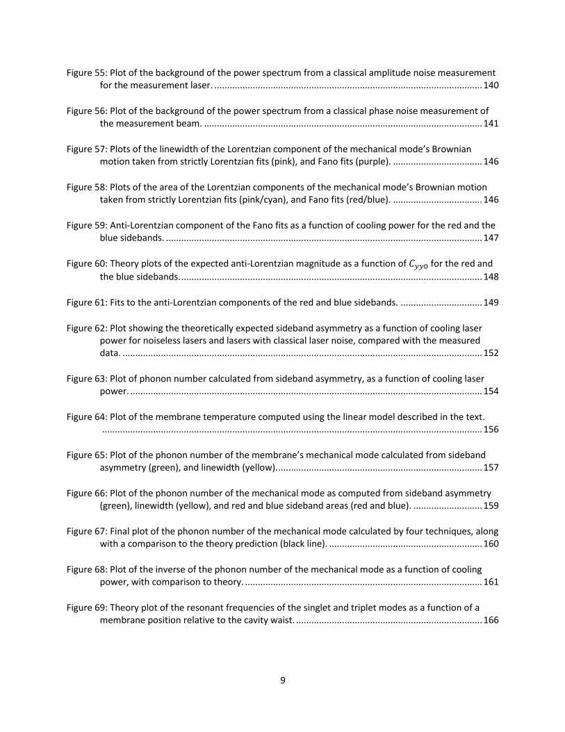
9

Figure 55: Plot of the background of the power spectrum from a classical amplitude noise measurement for the measurement laser. ......................................................................................................... 140

Figure 56: Plot of the background of the power spectrum from a classical phase noise measurement of the measurement beam. ............................................................................................................. 141

Figure 57: Plots of the linewidth of the Lorentzian component of the mechanical mode’s Brownian motion taken from strictly Lorentzian fits (pink), and Fano fits (purple). ................................... 146

Figure 58: Plots of the area of the Lorentzian components of the mechanical mode’s Brownian motion taken from strictly Lorentzian fits (pink/cyan), and Fano fits (red/blue). ................................... 146

Figure 59: Anti-Lorentzian component of the Fano fits as a function of cooling power for the red and the blue sidebands. ............................................................................................................................ 147

Figure 60: Theory plots of the expected anti-Lorentzian magnitude as a function of 𝐶𝑦𝑦0 for the red and

the blue sidebands. ...................................................................................................................... 148

Figure 61: Fits to the anti-Lorentzian components of the red and blue sidebands. ................................ 149

Figure 62: Plot showing the theoretically expected sideband asymmetry as a function of cooling laser power for noiseless lasers and lasers with classical laser noise, compared with the measured data. ............................................................................................................................................. 152

Figure 63: Plot of phonon number calculated from sideband asymmetry, as a function of cooling laser power. .......................................................................................................................................... 154

Figure 64: Plot of the membrane temperature computed using the linear model described in the text. ..................................................................................................................................................... 156

Figure 65: Plot of the phonon number of the membrane’s mechanical mode calculated from sideband asymmetry (green), and linewidth (yellow). ................................................................................ 157

Figure 66: Plot of the phonon number of the mechanical mode as computed from sideband asymmetry (green), linewidth (yellow), and red and blue sideband areas (red and blue). ........................... 159

Figure 67: Final plot of the phonon number of the mechanical mode calculated by four techniques, along with a comparison to the theory prediction (black line). ............................................................ 160

Figure 68: Plot of the inverse of the phonon number of the mechanical mode as a function of cooling power, with comparison to theory. ............................................................................................. 161

Figure 69: Theory plot of the resonant frequencies of the singlet and triplet modes as a function of a membrane position relative to the cavity waist. ......................................................................... 166

10

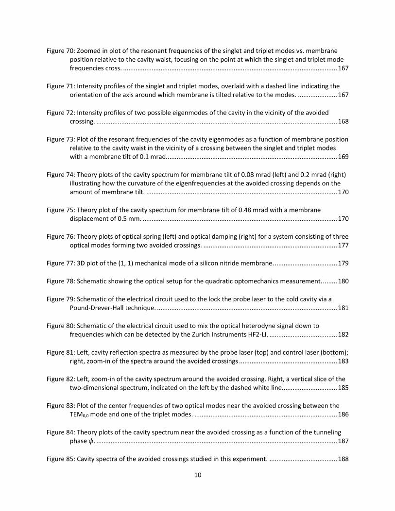
Figure 70: Zoomed in plot of the resonant frequencies of the singlet and triplet modes vs. membrane position relative to the cavity waist, focusing on the point at which the singlet and triplet mode frequencies cross. ........................................................................................................................ 167

Figure 71: Intensity profiles of the singlet and triplet modes, overlaid with a dashed line indicating the orientation of the axis around which membrane is tilted relative to the modes. ...................... 167

Figure 72: Intensity profiles of two possible eigenmodes of the cavity in the vicinity of the avoided crossing. ....................................................................................................................................... 168

Figure 73: Plot of the resonant frequencies of the cavity eigenmodes as a function of membrane position relative to the cavity waist in the vicinity of a crossing between the singlet and triplet modes with a membrane tilt of 0.1 mrad. ............................................................................................... 169

Figure 74: Theory plots of the cavity spectrum for membrane tilt of 0.08 mrad (left) and 0.2 mrad (right) illustrating how the curvature of the eigenfrequencies at the avoided crossing depends on the amount of membrane tilt. ........................................................................................................... 170

Figure 75: Theory plot of the cavity spectrum for membrane tilt of 0.48 mrad with a membrane displacement of 0.5 mm. ............................................................................................................. 170

Figure 76: Theory plots of optical spring (left) and optical damping (right) for a system consisting of three optical modes forming two avoided crossings. ........................................................................... 177

Figure 77: 3D plot of the (1, 1) mechanical mode of a silicon nitride membrane. ................................... 179

Figure 78: Schematic showing the optical setup for the quadratic optomechanics measurement. ........ 180

Figure 79: Schematic of the electrical circuit used to the lock the probe laser to the cold cavity via a Pound-Drever-Hall technique. ..................................................................................................... 181

Figure 80: Schematic of the electrical circuit used to mix the optical heterodyne signal down to frequencies which can be detected by the Zurich Instruments HF2-LI. ...................................... 182

Figure 81: Left, cavity reflection spectra as measured by the probe laser (top) and control laser (bottom); right, zoom-in of the spectra around the avoided crossings ....................................................... 183

Figure 82: Left, zoom-in of the cavity spectrum around the avoided crossing. Right, a vertical slice of the two-dimensional spectrum, indicated on the left by the dashed white line. .............................. 185

Figure 83: Plot of the center frequencies of two optical modes near the avoided crossing between the TEM0,0 mode and one of the triplet modes. ................................................................................ 186

Figure 84: Theory plots of the cavity spectrum near the avoided crossing as a function of the tunneling phase 𝜙. ....................................................................................................................................... 187

Figure 85: Cavity spectra of the avoided crossings studied in this experiment. ...................................... 188

11

Figure 86: Left, zoom-in of the cavity spectrum around the avoided crossing with green dashed line showing the region over which the control laser was stepped. Right, a theory plot of the avoided crossing generated from the parameters extracted as described above. ................................... 190

Figure 87: Left, color plot of Brownian motion power spectral densities of the membrane measured as the control laser was stepped across the avoided crossing. Right, color plot of the Brownian motion as predicted by theory. ................................................................................................... 191

Figure 88: A zoomed-in plot of the cavity spectrum with dashed lines representing the range over which the control laser was stepped at various membrane positions around the avoided crossing. ... 192

Figure 89: Left, plot of the optical spring of the mechanical mode as a function of laser detuning. Right, plot of optical damping of the mechanical mode as a function of laser detuning. ..................... 193

Figure 90: Left, plot of the optical spring of the mechanical mode as a function of laser detuning for various control beam powers. Right, plot of optical damping of the mechanical mode as a function of laser detuning for various control beam powers. ..................................................... 195

Figure 91: Plots comparing fitted membrane positions and control laser powers with their intended values. .......................................................................................................................................... 196

Figure 92: Plot of mechanical frequency shift as a function of laser detuning for three different avoided crossings. ...................................................................................................................................... 197

Figure 93: Schematic of the electrical circuit used for the phase-locked loop measurement. ................ 200

Figure 94: Power spectral density of the membrane’s frequency deviation............................................ 201

Figure 95: Plot of the maximum frequency deviation due to the optical spring effect caused by periodic modulation of the intracavity photon number. ........................................................................... 202

12

Table of Symbols

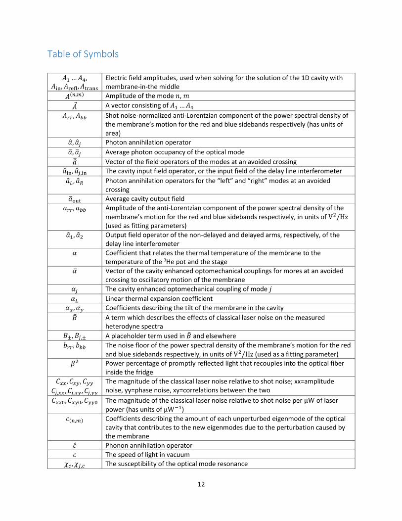
𝐴1…𝐴4, 𝐴in, 𝐴refl, 𝐴trans

Electric field amplitudes, used when solving for the solution of the 1D cavity with membrane-in-the middle

𝐴(𝑛,𝑚) Amplitude of the mode 𝑛, 𝑚

𝐴 A vector consisting of 𝐴1…𝐴4

𝐴𝑟𝑟, 𝐴𝑏𝑏 Shot noise-normalized anti-Lorentzian component of the power spectral density of the membrane’s motion for the red and blue sidebands respectively (has units of area)

��, ��𝑗 Photon annihilation operator

��, ��𝑗 Average photon occupancy of the optical mode

�� Vector of the field operators of the modes at an avoided crossing

��in, ��𝑗,in The cavity input field operator, or the input field of the delay line interferometer

��𝐿 , ��𝑅 Photon annihilation operators for the “left” and “right” modes at an avoided crossing

��out Average cavity output field

𝑎𝑟𝑟, 𝑎𝑏𝑏 Amplitude of the anti-Lorentzian component of the power spectral density of the membrane’s motion for the red and blue sidebands respectively, in units of V2/Hz (used as fitting parameters)

��1, ��2 Output field operator of the non-delayed and delayed arms, respectively, of the delay line interferometer

𝛼 Coefficient that relates the thermal temperature of the membrane to the temperature of the 3He pot and the stage

�� Vector of the cavity enhanced optomechanical couplings for mores at an avoided crossing to oscillatory motion of the membrane

𝛼𝑗 The cavity enhanced optomechanical coupling of mode 𝑗

𝛼𝐿 Linear thermal expansion coefficient

𝛼𝑥 , 𝛼𝑦 Coefficients describing the tilt of the membrane in the cavity

�� A term which describes the effects of classical laser noise on the measured heterodyne spectra

𝐵±, 𝐵𝑗,± A placeholder term used in �� and elsewhere

𝑏𝑟𝑟, 𝑏𝑏𝑏 The noise floor of the power spectral density of the membrane’s motion for the red and blue sidebands respectively, in units of V2/Hz (used as a fitting parameter)

𝛽2 Power percentage of promptly reflected light that recouples into the optical fiber inside the fridge

𝐶𝑥𝑥, 𝐶𝑥𝑦, 𝐶𝑦𝑦

𝐶𝑗,𝑥𝑥, 𝐶𝑗,𝑥𝑦, 𝐶𝑗,𝑦𝑦

The magnitude of the classical laser noise relative to shot noise; xx=amplitude noise, yy=phase noise, xy=correlations between the two

𝐶𝑥𝑥0, 𝐶𝑥𝑦0, 𝐶𝑦𝑦0 The magnitude of the classical laser noise relative to shot noise per μW of laser power (has units of μW−1)

𝑐(𝑛,𝑚) Coefficients describing the amount of each unperturbed eigenmode of the optical cavity that contributes to the new eigenmodes due to the perturbation caused by the membrane

�� Phonon annihilation operator

𝑐 The speed of light in vacuum

𝜒𝑐 , 𝜒𝑗,𝑐 The susceptibility of the optical mode resonance

13

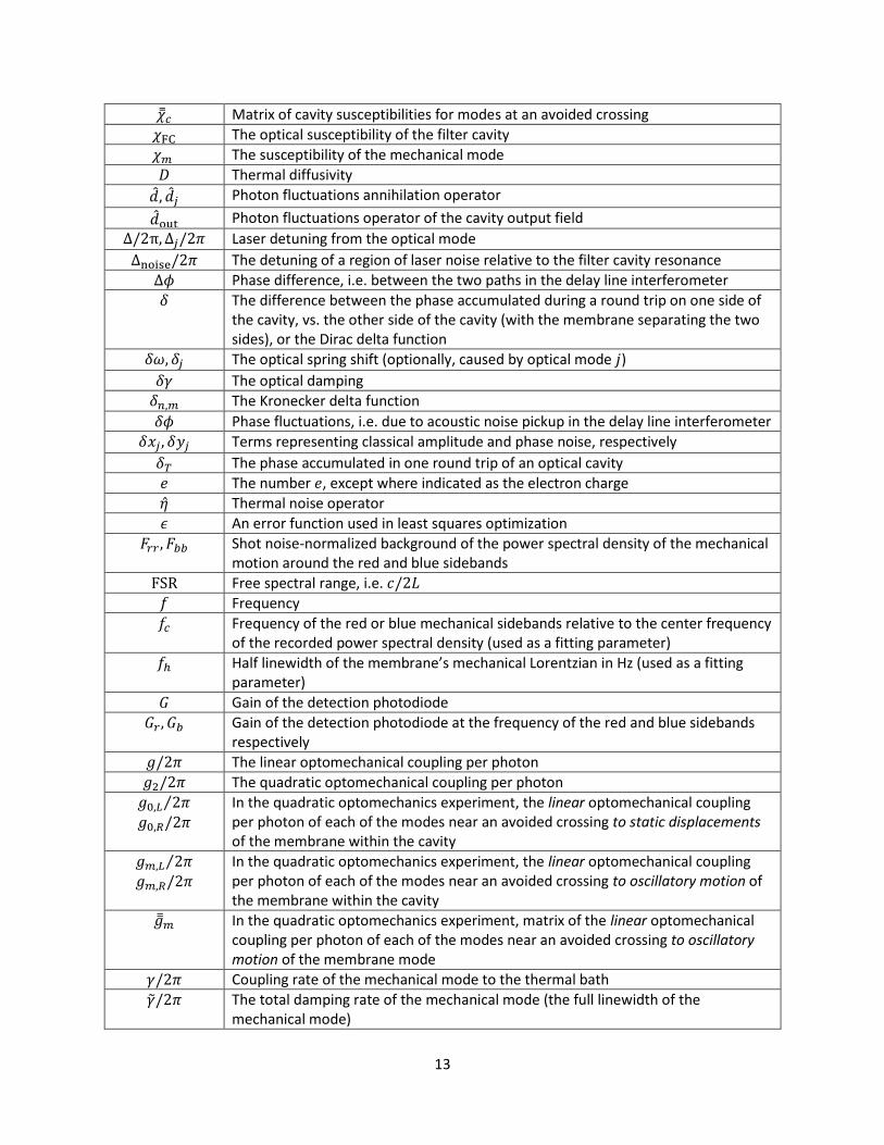
��𝑐 Matrix of cavity susceptibilities for modes at an avoided crossing

𝜒FC The optical susceptibility of the filter cavity

𝜒𝑚 The susceptibility of the mechanical mode

𝐷 Thermal diffusivity

��, ��𝑗 Photon fluctuations annihilation operator

��out Photon fluctuations operator of the cavity output field

Δ/2π, Δ𝑗/2𝜋 Laser detuning from the optical mode

Δnoise/2𝜋 The detuning of a region of laser noise relative to the filter cavity resonance

Δ𝜙 Phase difference, i.e. between the two paths in the delay line interferometer

𝛿 The difference between the phase accumulated during a round trip on one side of the cavity, vs. the other side of the cavity (with the membrane separating the two sides), or the Dirac delta function

𝛿𝜔, 𝛿𝑗 The optical spring shift (optionally, caused by optical mode 𝑗)

𝛿𝛾 The optical damping

𝛿𝑛,𝑚 The Kronecker delta function

𝛿𝜙 Phase fluctuations, i.e. due to acoustic noise pickup in the delay line interferometer

𝛿𝑥𝑗, 𝛿𝑦𝑗 Terms representing classical amplitude and phase noise, respectively

𝛿𝑇 The phase accumulated in one round trip of an optical cavity

𝑒 The number 𝑒, except where indicated as the electron charge

�� Thermal noise operator

𝜖 An error function used in least squares optimization

𝐹𝑟𝑟, 𝐹𝑏𝑏 Shot noise-normalized background of the power spectral density of the mechanical motion around the red and blue sidebands

FSR Free spectral range, i.e. 𝑐/2𝐿

𝑓 Frequency

𝑓𝑐 Frequency of the red or blue mechanical sidebands relative to the center frequency of the recorded power spectral density (used as a fitting parameter)

𝑓ℎ Half linewidth of the membrane’s mechanical Lorentzian in Hz (used as a fitting parameter)

𝐺 Gain of the detection photodiode

𝐺𝑟, 𝐺𝑏 Gain of the detection photodiode at the frequency of the red and blue sidebands respectively

𝑔/2𝜋 The linear optomechanical coupling per photon

𝑔2/2𝜋 The quadratic optomechanical coupling per photon

𝑔0,𝐿 2𝜋⁄ 𝑔0,𝑅/2𝜋

In the quadratic optomechanics experiment, the linear optomechanical coupling per photon of each of the modes near an avoided crossing to static displacements of the membrane within the cavity

𝑔𝑚,𝐿 2𝜋⁄

𝑔𝑚,𝑅/2𝜋

In the quadratic optomechanics experiment, the linear optomechanical coupling per photon of each of the modes near an avoided crossing to oscillatory motion of the membrane within the cavity

��𝑚 In the quadratic optomechanics experiment, matrix of the linear optomechanical coupling per photon of each of the modes near an avoided crossing to oscillatory motion of the membrane mode

𝛾/2𝜋 Coupling rate of the mechanical mode to the thermal bath

��/2𝜋 The total damping rate of the mechanical mode (the full linewidth of the mechanical mode)

14

𝛾𝑗/2𝜋 The optical damping of the mechanical mode due to optical mode 𝑗

𝐻 Hamiltonian

𝐻int Interaction Hamiltonian

𝐻intlin Linearized interaction Hamiltonian

𝐻diss, 𝐻drive Hamiltonian components representing dissipation and the laser drive

𝐻env Hamiltonian component representing the interaction with the environment

ℏ Reduced Planck constant

𝐼 Photon flux operator, i.e. the number operator of the cavity output field

𝐼 Identity matrix

𝑖 Imaginary unit, or photocurrent

𝑗 Subscript placeholder to indicate either the measurement beam mode 𝑠 or the cooling beam mode 𝑝

𝐾2, 𝐾𝑗2 Optical power in units of photons per second

𝑘 Wave vector

𝑘B Boltzmann’s constant

𝑘min For an optical fiber, 2.405 divided by the radius of the fiber cladding; this is approximately the minimum wave vector at which the cladding supports at least one optical mode

𝑘max For an optical fiber, 2 divided by the mode field radius; this is approximately the maximum wave vector at which the core supports single-mode propagation

𝑘(𝑛,𝑚)(0)

The wave vector of the mode 𝑛, 𝑚 for the unperturbed cavity, used when calculating the perturbation due to the membrane

𝜅/2𝜋, 𝜅𝑗/2𝜋 Total decay rate of the optical mode (the full linewidth of the optical resonance)

�� Matrix containing the 𝜅’s of modes at an avoided crossing

𝜅in 2𝜋⁄ 𝜅𝑗,in/2𝜋

Decay rate of the optical mode through the cavity input mirror

√𝜅in Vector containing the square root of the 𝜅in’s of modes at an avoided crossing

𝜅int 2𝜋⁄ 𝜅𝑗,int/2𝜋

Decay rate of the optical mode due to losses within the cavity

𝐿 Length of the optical cavity, or length of one side of the membrane, or in the quadratic optomechanics experiment, a subscript indicating the “left” mode at an avoided crossing (generally the TEM0,0)

𝐿𝑑 Thickness of the membrane

𝐿𝑟𝑟, 𝐿𝑏𝑏 Shot noise-normalized area of the Lorentzian component of the power spectral density of the membrane’s motion for the red and blue sidebands respectively

𝐿1 Length from cavity input mirror to the membrane

𝐿2 Length from membrane to cavity output mirror

𝑙 Length of the fiber optic delay line in the delay line interferometer

Λ A diagonal matrix consisting of the eigenvalues of another matrix

𝜆 Wavelength of light, generally 1064 nm unless otherwise specified

𝑀 A generic symbol representing a matrix

𝑚 Mass, or a generic symbol for eigenvalues of a matrix, or arbitrary integer such as a mode index

𝑁 A placeholder in the cavity equations of motion

𝑛 Photon number, or index of refraction, or an arbitrary integer such as a mode index

𝑛int An arbitrary integer, for when 𝑚 and 𝑛 aren’t enough

15

𝑛𝑗 Effective phonon number of the optical mode 𝑗, in the sense of the phonon number the mechanical mode would have if in thermal equilibrium with the optical drive

𝑛𝑚 Phonon number

𝑛𝑚(𝑛,𝑚)

Phonon number of mode 𝑛, 𝑚

𝑛𝑚(𝛾)

Phonon number calculated from the linewidth of the mechanical sidebands

𝑛𝑚(𝜉′)

Phonon number calculated from the sideband asymmetry

𝑛𝑚(𝑟𝑟)

, 𝑛𝑚(𝑏𝑏)

Phonon number calculated from the displacement-calibrated area under the red or blue sidebands respectively

𝑛SiN Index of refraction of silicon nitride

𝑛th Thermal phonon number of the mechanical mode

∇2 Laplacian operator

𝜈 Optical frequency

𝑃 Optical power, or a parameter in the theory of Gaussian laser beams related to the phase of the beam

𝑃circ The circulating power in the optical cavity

𝑃𝑗, 𝑃LO Optical power in the beam driving mode 𝑗, or in the local oscillator beam, respectively

𝑝 Subscript indicating the cooling beam mode

𝜙 A general symbol for phase, sometimes used in more specific contexts

𝜙(𝑛,𝑚) The phase of mode 𝑛, 𝑚

Φ The Guoy phase

𝜋 Pi

𝜓 A component of the solution to the scalar wave equation

𝑄 Mechanical quality factor, or a matrix consisting of the eigenvalues of another matrix

𝑞 Parameter in the theory of Gaussian laser beams related to the cross sectional profile of the beam

𝑞0 𝑞 evaluated at the beam waist

𝑅 Radius of curvature of the phase front of a Gaussian beam, or power reflectivity of a cavity mirror, or responsivity of the measurement photodiode, or in the quadratic optomechanics experiment, a subscript indicating the “right” mode at an avoided crossing

𝑅1, 𝑅2 In the quadratic optomechanics experiment, subscripts used to differentiate between additional modes at an avoided crossing

𝑅mirror Radius of curvature of the cavity mirrors

𝑟 Ratio of the local oscillator power to the measurement beam power

��𝑑 Complex field reflectivity of the membrane

𝑟𝑑 Magnitude of ��𝑑

𝑟1, 𝑟2 Field reflectivities of the cavity input and output mirrors, respectively

𝜌, 𝜌𝑝 Normalized amplitude of the reflected measurement beam and cooling beam respectively after interacting with the cavity

𝑆 Power spectral density

𝑆(𝑛) The power spectral density of either sideband of the membrane’s motion computed from the 𝑛th recorded time trace

𝑆avg(𝑛) The average power spectral density of the either sideband of the membrane’s

motion computed after recording 𝑛 time traces

16

𝑆𝑟𝑟, 𝑆𝑏𝑏 Power spectral density of the membrane’s motion for the red and blue sidebands respectively

𝑆𝑟𝑟,𝑝, 𝑆𝑏𝑏,𝑝 Contribution of the cooling beam (shot noise) to 𝑆𝑟𝑟 and 𝑆𝑏𝑏

𝑆𝜙𝜙 Power spectral density of phase noise due to thermal fluctuations in the delay line interferometer

𝑠 Subscript indicating the measurement beam mode

𝑠𝑟𝑟, 𝑠𝑏𝑏 Amplitude of the Lorentzian component of the red and blue mechanical sidebands respectively in the power spectral density of the membrane’s motion, in units of V2/Hz (used as a fitting parameter)

Σ The optomechanical self energy

𝜎 The detection efficiency of the measurement photodiode

𝜎QE The quantum efficiency of the measurement photodiode

𝑇 Absolute temperature

𝑇tot, 𝑇ff, 𝑇99 𝑇99→cir, 𝑇cir

Respective power transmissivities of: all optical components after the circulator, the splice to the fridge fiber, the 99% output port of the 99:1 beamsplitter, the splice between the 99:1 beamsplitter and the circulator, and the circulator itself. See Table 1 on page 129.

𝑇stage, 𝑇pot Absolute temperature of the stage and the 3He pot respectively

𝑡 Time, or the thickness of the membrane (equivalent to 𝐿𝑑), or the coupling between two modes at an avoided crossing

��𝑑 Complex field transmissivity of the membrane

𝑡𝑑 Magnitude of ��𝑑

𝑡1, 𝑡2 Field transmissivities of the cavity input and output mirrors, respectively

𝜏 A delay time, or a ringdown time

𝜏meas The length of time over which a measurement was taken

Θ The Heaviside step function

𝜃 Phase of the local oscillator beam relative to the measurement beam

𝑢 Solution to the scalar wave equation

𝑢(𝑛,𝑚)(0) The unperturbed eigenmodes of the Fabry-Perot cavity, used when calculating the

effects of the perturbation due to the membrane

𝑉 A perturbation to the free-space scalar wave equation

𝑉(𝑛,𝑚) The expectation value of the perturbation 𝑉 for the modes 𝑛, 𝑚, i.e.:

⟨𝑢𝑛,𝑚(0)|𝑉|𝑢𝑛,𝑚

(0) ⟩

𝑊𝑟𝑟 ,𝑊𝑏𝑏 The red and blue sideband “weights”, which are normalized versions of 𝐿𝑟𝑟 and 𝐿𝑏𝑏

𝑤 Radius of a Gaussian laser beam

𝑤0 Radius of Gaussian laser beam at the beam waist, or if in a fiber, the mode field radius

Ω𝐿 , Ω𝑗 Drive laser angular frequency

𝜔 Angular frequency

𝜔𝑐 , 𝜔𝑗 Angular frequency of the optical cavity mode

��𝑐 Matrix describing the resonant angular frequencies of, and couplings between modes at an avoided crossing

𝜔𝑐′ , 𝜔𝑐

′′ First and second derivatives of the cavity’s resonant frequency as a function of membrane position

𝜔if Frequency of the heterodyne beat note

17

𝜔𝑚 Angular frequency of the mechanical mode

��𝑚 Angular frequency of the mechanical mode as perturbed by the lasers

𝜔𝑚(𝑛,𝑚) Angular frequency of the 𝑛, 𝑚 mechanical mode

𝜔𝑟 , 𝜔𝑏 Angular frequency of the red and blue mechanical sidebands in the power spectral density of the membrane’s motion

𝜔0 Angular frequency at which there is an avoided crossing in the optical cavity spectrum

𝑥 Except where defined differently, the dimensionless position operator of the mechanical mode

𝑥zpf Amplitude of the mechanical mode’s zero-point fluctuations

��𝜙 Amplitude of one quadrature of the oscillator’s position operator

𝜉, 𝜉𝑗 Vacuum noise of the optical mode, or the sideband asymmetry (red/blue)

𝜉′ Time derivative of the vacuum noise of the optical mode, or the gain and detuning-corrected sideband asymmetry

𝜉𝑗,in Vacuum noise of the laser driving mode 𝑗

𝜉1, 𝜉2 Vacuum noise of the fields in the non-delayed and delayed arms, respectively, of the delay line interferometer

��𝜙 Amplitude of another quadrature of the oscillator’s position operator

�� Except where defined differently, the dimensionless position operator of the mechanical mode (�� is used in place of 𝑥 for the chapter on Quadratic Optomechanics to be consistent with our prior publication on the subject)

𝑧zpf Amplitude of the mechanical mode’s zero-point fluctuations

𝑧𝑐 An equation describing the orientation of the membrane within the cavity

𝑧0 The position of the membrane in the cavity

𝜁𝑗 A placeholder in the cavity equations of motion

18

I. Introduction

1. An Historical Anecdote

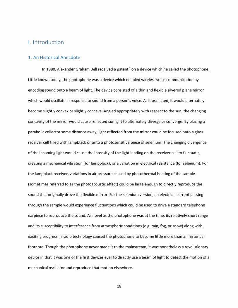
In 1880, Alexander Graham Bell received a patent 1 on a device which he called the photophone.

Little known today, the photophone was a device which enabled wireless voice communication by

encoding sound onto a beam of light. The device consisted of a thin and flexible silvered plane mirror

which would oscillate in response to sound from a person’s voice. As it oscillated, it would alternately

become slightly convex or slightly concave. Angled appropriately with respect to the sun, the changing

concavity of the mirror would cause reflected sunlight to alternately diverge or converge. By placing a

parabolic collector some distance away, light reflected from the mirror could be focused onto a glass

receiver cell filled with lampblack or onto a photosensitive piece of selenium. The changing divergence

of the incoming light would cause the intensity of the light landing on the receiver cell to fluctuate,

creating a mechanical vibration (for lampblack), or a variation in electrical resistance (for selenium). For

the lampblack receiver, variations in air pressure caused by photothermal heating of the sample

(sometimes referred to as the photoacoustic effect) could be large enough to directly reproduce the

sound that originally drove the flexible mirror. For the selenium version, an electrical current passing

through the sample would experience fluctuations which could be used to drive a standard telephone

earpiece to reproduce the sound. As novel as the photophone was at the time, its relatively short range

and its susceptibility to interference from atmospheric conditions (e.g. rain, fog, or snow) along with

exciting progress in radio technology caused the photophone to become little more than an historical

footnote. Though the photophone never made it to the mainstream, it was nonetheless a revolutionary

device in that it was one of the first devices ever to directly use a beam of light to detect the motion of a

mechanical oscillator and reproduce that motion elsewhere.

19

Figure 1: Photophone transmitter (left) 2, and receiver (right) 3

While the scientific principles upon which Bell’s photophone was based differ from the

principles upon which modern optomechanics is based, many of themes are the same. Modern

optomechanical experiments involve a mechanical oscillator which modulates the phase of a beam of

light as it oscillates, just as the photophone modulated the convergence of a beam of light, and hence

the intensity landing on a photoreceiver. Many experiments today also focus on coupling oscillators

together using light as a coupling mechanism, just as the photophone coupled the vibrations of granular

lampblack to the vibrations of the flexible mirror. Electro-opto-mechanical devices today attempt to

transfer electrical (microwave) signals in a quantum coherent manner using mechanical oscillators as

up/down-converters to and from optical frequencies, just as the photophone paired with a speaker at

the transmitter could have conceivably upconverted audio frequency electrical signals to the optical

regime and back again with a selenium receiver on the other end.

2. Modern Optomechanics

The modern field of optomechanics seeks to harness mechanical interactions with light to both

control and measure the motion of mechanical oscillators with extremely high precision. Some goals of

modern optomechanics include measurement of extremely small forces, displacements, and

accelerations, and detection of small masses. 4 The incredible sensitivity to these quantities obtained in

modern optomechanical systems allows for exploration of the quantum mechanical behaviors of

20

mechanical oscillators using light to both control and measure oscillators’ behavior. Modern

optomechanical systems can use the radiation pressure force to cool mechanical oscillators to their

vibrational ground states, 5 - 11 prepare mechanical oscillators in non-classical states, 5, 12, 13 and

coherently transfer states between mechanical oscillators and the light field. 14, 15 The long lifetimes of

mechanical states make them well suited for use as quantum memory elements, and the ability to

transfer states from mechanical oscillators to the light field and back brings about potential uses for

future quantum information processors. 16 The broadband nature of the coupling between mechanical

oscillators and electromagnetic fields also allows for coherent quantum state transfer between

electromagnetic modes of vastly different frequencies. On a more basic level, modern optomechanical

systems provide the tools needed to test predictions of quantum mechanics in macroscopic objects, and

even to explore the fundamental limits of measurement itself.

While Bell’s photophone was a novel invention for its time, the goals of modern optomechanics

require a more advanced system than a membrane mirror and some lampblack or a selenium

photoresistor. Unlike the photophone, the interaction between light and mechanical oscillators in

modern optomechanical systems is driven by radiation pressure. Radiation pressure is the force exerted

on any surface which absorbs or reflects light due to conservation of the momentum carried by the

electromagnetic fields that make up the light. For the purposes of building an optomechanical system,

radiation pressure is superior to the photoacoustic and photoresistive effects used in the photophone

for several reasons. First, the fact that radiation pressure can exert a force without being absorbed

means that in an appropriate system the same light can interact with a mechanical oscillator multiple

times, increasing the strength of the radiation pressure force. During each of these multiple interactions,

the light acquires information about the state of the oscillator, allowing for detection of the oscillator’s

state. Additionally, since slow thermal excitations or high latency photoresistive responses are not

21

required for the mechanical oscillator to respond to the light, the bandwidth of the interaction is much

higher than can be achieved via the photoacoustic effect.

3. Basic Optomechanical Effects

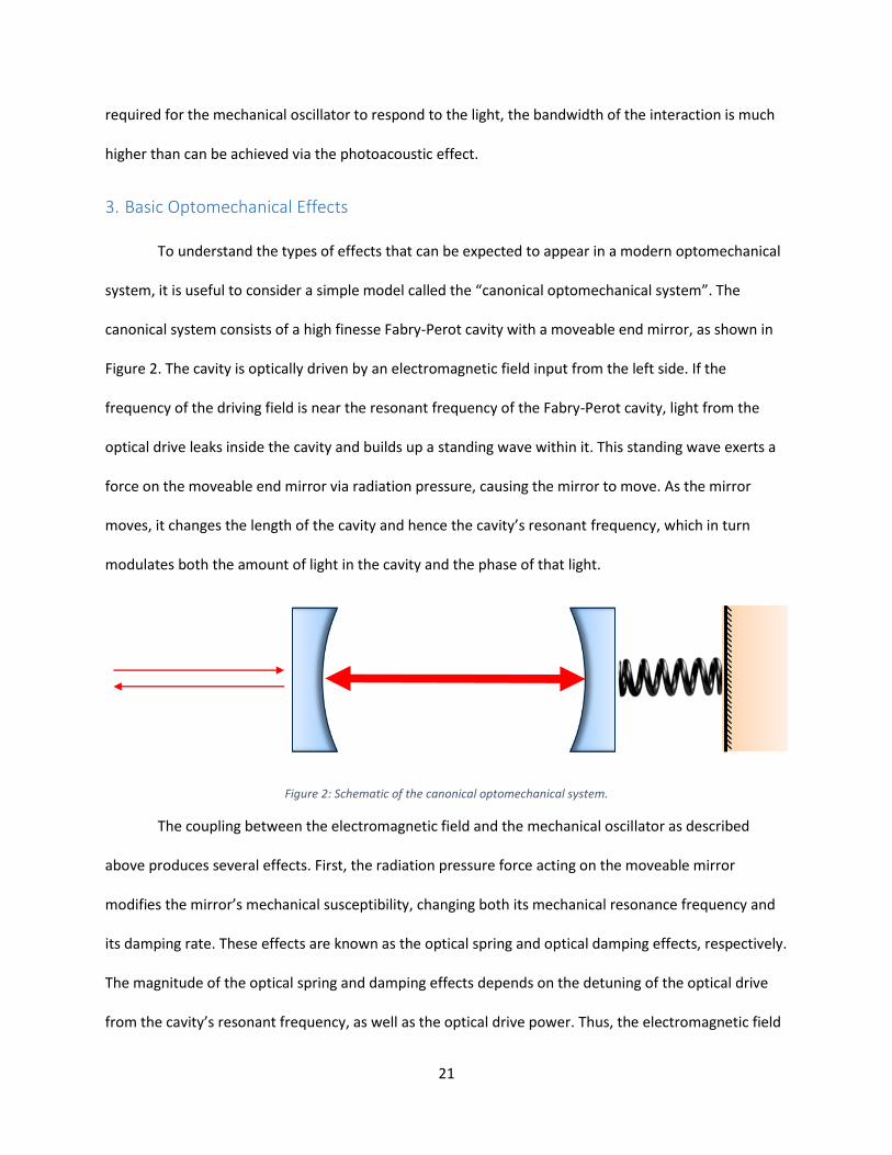
To understand the types of effects that can be expected to appear in a modern optomechanical

system, it is useful to consider a simple model called the “canonical optomechanical system”. The

canonical system consists of a high finesse Fabry-Perot cavity with a moveable end mirror, as shown in

Figure 2. The cavity is optically driven by an electromagnetic field input from the left side. If the

frequency of the driving field is near the resonant frequency of the Fabry-Perot cavity, light from the

optical drive leaks inside the cavity and builds up a standing wave within it. This standing wave exerts a

force on the moveable end mirror via radiation pressure, causing the mirror to move. As the mirror

moves, it changes the length of the cavity and hence the cavity’s resonant frequency, which in turn

modulates both the amount of light in the cavity and the phase of that light.

Figure 2: Schematic of the canonical optomechanical system.

The coupling between the electromagnetic field and the mechanical oscillator as described

above produces several effects. First, the radiation pressure force acting on the moveable mirror

modifies the mirror’s mechanical susceptibility, changing both its mechanical resonance frequency and

its damping rate. These effects are known as the optical spring and optical damping effects, respectively.

The magnitude of the optical spring and damping effects depends on the detuning of the optical drive

from the cavity’s resonant frequency, as well as the optical drive power. Thus, the electromagnetic field

22

can be used to control the motion of the mechanical oscillator. A second consequence of the

optomechanical coupling is that the changing cavity length caused by the motion of the mirror produces

modulation in the optical field. This modulation carries away information about the mirror’s motion. In

this way, the electromagnetic field can also be used to measure the oscillator’s motion.

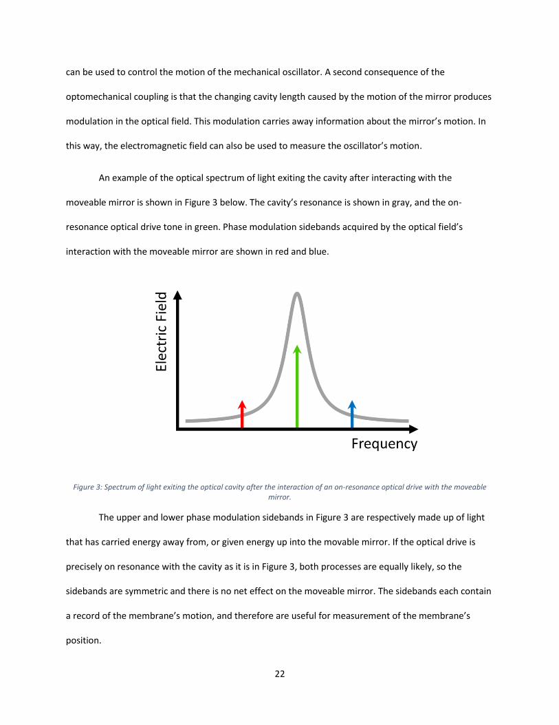
An example of the optical spectrum of light exiting the cavity after interacting with the

moveable mirror is shown in Figure 3 below. The cavity’s resonance is shown in gray, and the on-

resonance optical drive tone in green. Phase modulation sidebands acquired by the optical field’s

interaction with the moveable mirror are shown in red and blue.

Figure 3: Spectrum of light exiting the optical cavity after the interaction of an on-resonance optical drive with the moveable mirror.

The upper and lower phase modulation sidebands in Figure 3 are respectively made up of light

that has carried energy away from, or given energy up into the movable mirror. If the optical drive is

precisely on resonance with the cavity as it is in Figure 3, both processes are equally likely, so the

sidebands are symmetric and there is no net effect on the moveable mirror. The sidebands each contain

a record of the membrane’s motion, and therefore are useful for measurement of the membrane’s

position.

23

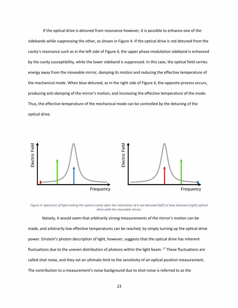
If the optical drive is detuned from resonance however, it is possible to enhance one of the

sidebands while suppressing the other, as shown in Figure 4. If the optical drive is red detuned from the

cavity’s resonance such as in the left side of Figure 4, the upper phase modulation sideband is enhanced

by the cavity susceptibility, while the lower sideband is suppressed. In this case, the optical field carries

energy away from the moveable mirror, damping its motion and reducing the effective temperature of

the mechanical mode. When blue detuned, as in the right side of Figure 4, the opposite process occurs,

producing anti-damping of the mirror’s motion, and increasing the effective temperature of the mode.

Thus, the effective temperature of the mechanical mode can be controlled by the detuning of the

optical drive.

Figure 4: Spectrum of light exiting the optical cavity after the interaction of a red detuned (left) or blue detuned (right) optical drive with the moveable mirror.

Naively, it would seem that arbitrarily strong measurements of the mirror’s motion can be

made, and arbitrarily low effective temperatures can be reached, by simply turning up the optical drive

power. Einstein’s photon description of light, however, suggests that the optical drive has inherent

fluctuations due to the uneven distribution of photons within the light beam. 17 These fluctuations are

called shot noise, and they set an ultimate limit to the sensitivity of an optical position measurement.

The contribution to a measurement’s noise background due to shot noise is referred to as the

24

measurement imprecision. Measurement imprecision scales inversely with the total power of the optical

beam used to perform a measurement. However, as the power of the measurement beam is turned up,

the amount of radiation pressure the beam exerts on the mirror increases as well. Fluctuations in the

radiation pressure caused by the shot noise fluctuations in the light beam can then drive the mechanical

oscillator, creating fluctuations in its position. These fluctuations are referred to generically as the

measurement back-action, or more specifically in this case, as measurement back-action due to

radiation pressure shot noise. Radiation pressure shot noise sets another limit to the sensitivity of an

optical position measurement, and it increases proportionally with the total power of the optical beam

used to perform the measurement. Thus, in any optomechanical position measurement there is a

compromise between measurement imprecision and measurement back-action due to radiation

pressure shot noise of the beam used to perform the measurement. There exists an optimal point at

which the sum of the measurement imprecision and the back-action is minimized. This point is called

the standard quantum limit, and represents the maximally sensitive position measurement possible in

an optomechanical system without employing special techniques to evade the back-action of the

measurement. 4, 18, 19 In addition to setting limits on measurement sensitivity, radiation pressure shot

noise also limits the amount of cooling that can be done using sideband cooling techniques. 20

Many modern optomechanical systems operate in a regime where the effects of radiation

pressure shot noise are significant. For example, the phase modulation sidebands produced by the

interaction between an on-resonance optical drive and a mechanical oscillator that has been cooled

close to its quantum vibrational ground state are expected to show asymmetry which can be attributed

in part to the fact that the radiation pressure shot noise from the optical field used for measurement is

correlated with the shot noise of the light exiting the optical cavity. 21 This sideband asymmetry is

significant because it provides evidence of the quantized nature of the electromagnetic field in the

cavity, and can be used as a probe of the effective temperature of the mechanical mode. Other

25

experiments have reached the regime where the measurement’s sensitivity to the position of the

mechanical oscillator is dominated by back-action from radiation pressure shot noise rather than the

measurement imprecision, 22 which similarly provides evidence of the quantization of the

electromagnetic field within the cavity and confirms predictions 19 that radiation pressure shot noise can

affect the motion of mechanical oscillators.

While radiation pressure limits the precision to which it is possible to measure a mechanical

oscillator’s position, this is not necessarily true for measurements of other characteristics of an

oscillator’s motion. Measurements which measure such characteristics are called quantum non-

demolition, or back-action evading measurements. These measurements involve measuring an

observable that commutes with the full Hamiltonian of the system. With such an observable, the back-

action caused by the measurement affects a quadrature of the motion that does not perturb the one

being measured. Thus, unlike position, it is possible to measure such a quantum non-demolition

observable to arbitrary precision. One example of this is a measurement of only one quadrature of the

oscillator’s position. For example, the position operator of a mechanical oscillator can be decomposed

into quadratures as follows:

𝑥(𝑡) = ��𝜙 cos(𝜔𝑚𝑡 + 𝜙) + ��𝜙 sin(𝜔𝑚𝑡 + 𝜙) (1)

In Equation (1), 𝜔𝑚/2𝜋 is the mechanical frequency of the oscillator, 𝑡 is time, 𝜙 is an arbitrary phase,

and ��𝜙 and ��𝜙 are the quadrature amplitudes. It can be shown that measurements of either only ��𝜙 or

only ��𝜙 can be made to arbitrary precision, and that back-action from measurement of either affects

only the other quadrature. 23 Such a measurement can be implemented, for example, by measuring the

oscillator’s position stroboscopically at times when one quadrature is maximized and the other is

minimized, 23 or through a reservoir engineering scheme in which two measurement tones are used to

achieve the same result in the steady state. 13 When a quantum non-demolition measurement is

26

performed in such a way as to measure one quadrature of motion to an uncertainty less than the

fluctuations caused by the oscillator’s zero-point motion, the mechanical oscillator is said to be in a

squeezed state. 23

From this brief description of optomechanical interactions, it is clear that optomechanical

systems are excellent tools for probing quantum behavior of mechanical oscillators, and also for

characterizing properties of quantum measurements. However, optomechanical systems also have

many practical uses beyond just testing the predictions of quantum mechanics itself. In the next section,

I will discuss some of these applications.

4. Applications of Optomechanics

The excellent displacement sensitivity of optomechanical systems makes them useful for

construction of precision accelerometers, where it is desirable to measure the motion of a test mass due

to weak forces or accelerations. Perhaps the largest examples of this are the Laser Interferometric

Gravitational Wave (LIGO) observatories, which use optomechanical systems consisting of Fabry-Perot

cavities with kilogram scale moveable mirrors, very similar to the canonical system, to detect tiny

displacements caused by passing gravitational waves. 24

In sensitive accelerometers such as LIGO, the standard quantum limit sets a bound on the

weakest forces and accelerations that can be detected. One way to improve sensitivity beyond the

standard quantum limit is by using squeezed light to perform the measurement. In the last section I

described how a quantum non-demolition measurement can reduce the fluctuations in one quadrature

of an oscillator’s motion to below the level of the oscillator’s zero-point fluctuations at the expense of

larger fluctuations in the other quadrature. Analogously, it is possible to reduce the fluctuations in one

quadrature of a light field to below the shot noise level at the expense of fluctuations in the other

quadrature. By reducing fluctuations in the amplitude quadrature of a light field below the shot noise

27

level, back-action due to the radiation pressure shot noise of that light acting on a mechanical oscillator

can be reduced. Optomechanical systems themselves are one way in which such squeezed light can be

produced. An optomechanical system whose position fluctuations are driven predominantly by the

radiation pressure shot noise of an on-resonance optical drive will produce phase modulation of the

intracavity optical field that is correlated with the shot noise in the amplitude quadrature. These

correlations can destructively interfere along the axis of some particular quadrature, reducing

fluctuations in such a quadrature to below the shot noise level. 25

Beyond sensitive displacement measurements, optomechanical systems are useful because they

can be used to store and transduce quantum information. I have already described how an

optomechanical system can prepare a mechanical oscillator in its vibrational ground state. From the

ground state, an oscillator can be excited into other states by the electromagnetic field. Under the right

conditions, it is possible to transfer the quantum state of the electromagnetic field into the mechanical

oscillator which can store it, acting like a quantum memory element. 16 The state that is stored in the

mechanical oscillator can then be transferred back into the electromagnetic field at a later time. The

ability to store, manipulate, and retrieve information is fundamental to the operation of a computer; the

ability of optomechanical systems to do these things with quantum states therefore makes them

promising candidates for future uses in quantum computing.

Another aspect of optomechanical systems which makes them particularly attractive for

quantum computing is the fact that mechanical oscillators can couple to electromagnetic radiation of

many different frequencies. Thus, for example, a quantum state can be transmitted on a microwave

signal within a quantum computer, stored in a mechanical oscillator via optomechanical interactions,

and then retrieved by an optical light pulse interacting with the same mechanical oscillator. 15, 16 The

optical light can then be transmitted a long distance via a low-loss optical fiber and stored into another

mechanical element at a remote location. Such transduction of quantum states between

28

electromagnetic modes of different frequencies, and also between mechanical memory elements which

can be physically separated by long distances, holds promise for future quantum networking.

Optomechanical systems which are specifically designed to couple to more than one type of

electromagnetic radiation are referred to as “hybrid” optomechanical systems.

It is clear that there are many practical applications of optomechanical systems, ranging from

putting their precision displacement sensitivity to use, to building fundamental components of quantum

computers. In the next section I will describe some of technical properties of practical optomechanical

systems, before giving a review of some of the experiments in the field.

5. Practical Optomechanical Systems

In the last several years, experiments characterizing the fundamental effects of optomechanics,

utilizing optomechanical systems to probe predictions of quantum mechanics, and demonstrating many

of the practical applications just mentioned, have been developed. The systems used in these

experiments operate using the same physical principles as the canonical system, but their designs often

differ in order to accommodate various practical requirements.

One common practical requirement is cryogenic compatibility. According to the correspondence

principle, a typical meso- or macro-scale mechanical oscillator at room temperature behaves classically.

In a quantum mechanical sense, this means that the oscillator exists in a mixed thermal state where it is

strongly entangled with and influenced by the thermal bath. Measurements of the instantaneous

phonon occupancy of the mechanical oscillator in a thermal state should recover values consistent with

the Maxwell-Boltzmann distribution. Due to the large spread of this distribution for room temperature

oscillators relative to the quantum of mechanical motion ℏ𝜔𝑚 and the frequent fluctuations in phonon

occupancy due to oscillator’s interaction with the thermal bath, it is difficult to make a measurement

strong enough to observe the quantization of the mechanical oscillator’s phonon number. Observation

29

of quantization in a mechanical oscillator therefore requires cooling the mechanical oscillator to the

point where the width of the Boltzmann distribution is closer to the size of the quantum of mechanical

motion. Since the standard deviation of the Maxwell-Boltzmann distribution for the energy of an

oscillator in a thermal state scales ∝ 𝑘B𝑇, this condition is approximately expressed as 𝑘B𝑇 ≈ ℏ𝜔𝑚.

Thus, the temperature to which a mechanical oscillator must be cooled to observe quantum effects

scales with the frequency of the mechanical oscillator. For oscillators in the GHz regime, the necessary

temperatures can be achieved using conventional cryogenic techniques. For example, a 1 GHz oscillator

would satisfy 𝑘B𝑇 ≈ ℏ𝜔𝑚 at a temperature of 50 mK, well within range of temperatures achievable with

a modern helium dilution refrigerator. For lower frequency oscillators, however, this criterion is much

more difficult to satisfy. A 1 MHz oscillator would have to be cooled to 50 μK, well beyond the reach of

conventional cryogenic refrigeration.

Optomechanical systems therefore typically must be designed with components that can

tolerate extremely cold temperatures. Both the mechanical oscillator itself and the system around it

such as the oscillator’s mount and the optics used to couple the electromagnetic field into the system

must be thermally stable and remain aligned over the range of temperatures from room temperature

down to the cryogenic realm. Additionally, it is desirable to select a mechanical oscillator with a high

intrinsic quality factor (as low a thermal damping rate as possible), so that the oscillator’s motion will be

dominated by its coupling to the optical drive, rather than the coupling to the thermal bath. Finally, the

oscillator must be well suited for control and measurement with an electromagnetic field. For this, the

mechanical oscillator must have low optical absorption at the frequencies chosen for the optical drive,

geometric compatibility with the optical cavity, and a low enough mass for the radiation pressure force

to have an appreciable effect.

While particular experiments may have other requirements, these are the general properties

that are desirable in most optomechanical systems. Simultaneously realizing all of these characteristics

30

in a system like the canonical system can be difficult, and therefore optomechanical systems come in a

diverse array of designs. Each system is tailored to the scientific goals of the experiment for which the

system is built. In the next section I will describe some of these systems, as well as the scientific goals

they have achieved.

6. Review of the Field

The field of optomechanics has truly blossomed within the last ten years, with optomechanical

systems of many different shapes and sizes achieving significant results. Systems that achieve ground

state cooling of macroscopic oscillators have been developed, as have systems that use mechanical

oscillators to detect radiation pressure shot noise. Yet other systems have prepared oscillators into non-

classical states of motion, and demonstrated coherent transfer of quantum states between mechanical

oscillators and the light field. In this section I will give a review of the first modern optomechanical

device, as well as some of these more recent papers, and discuss how each is relevant to the goals of the

modern field of optomechanics so that the reader might appreciate the progress the field has made, and

gain an understanding of how this dissertation sits in relation to the rest of the field.

The first modern optomechanical devices was Branginskiĭ, Manukin, and Tikhonov’s 1969

microwave cavity with a moveable wall. 26 A schematic illustration of the system, taken from the original

publication 26 is shown in Figure 5 below.

31

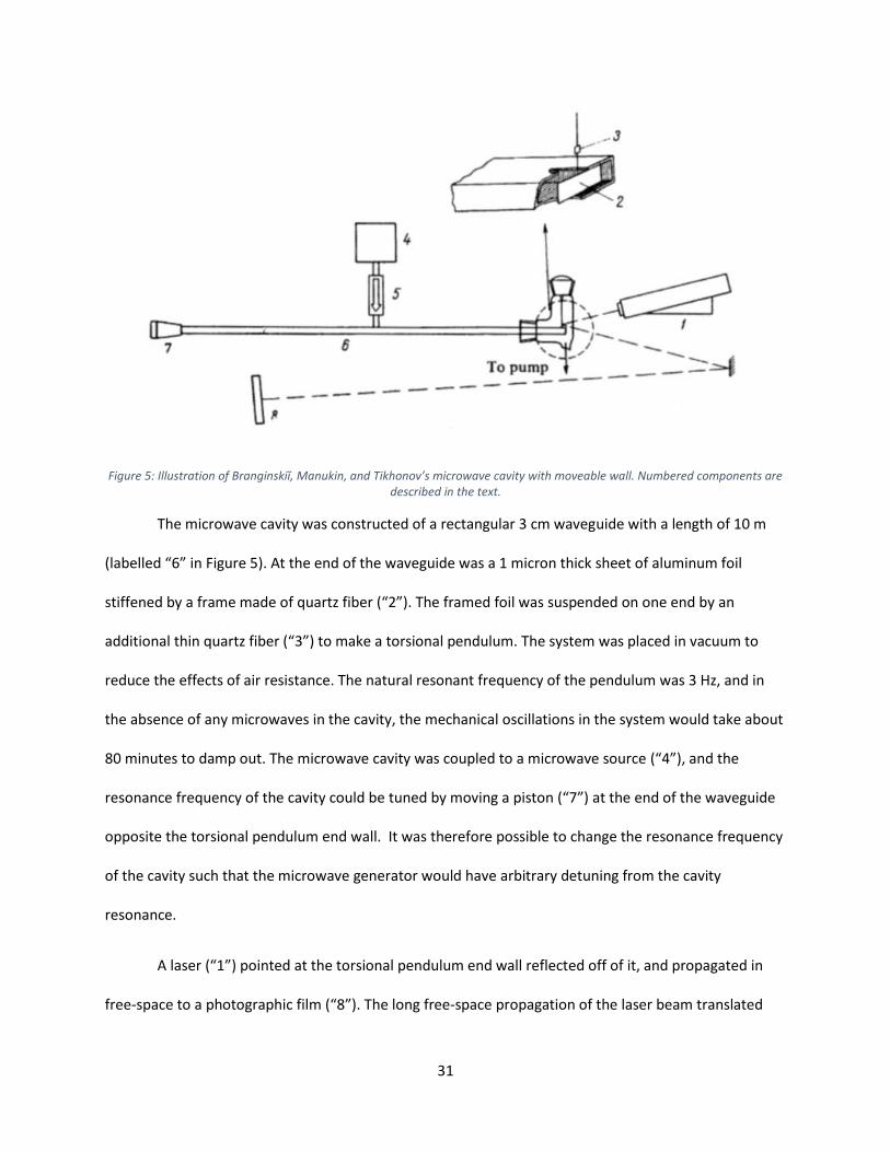
Figure 5: Illustration of Branginskiĭ, Manukin, and Tikhonov’s microwave cavity with moveable wall. Numbered components are described in the text.

The microwave cavity was constructed of a rectangular 3 cm waveguide with a length of 10 m

(labelled “6” in Figure 5). At the end of the waveguide was a 1 micron thick sheet of aluminum foil

stiffened by a frame made of quartz fiber (“2”). The framed foil was suspended on one end by an

additional thin quartz fiber (“3”) to make a torsional pendulum. The system was placed in vacuum to

reduce the effects of air resistance. The natural resonant frequency of the pendulum was 3 Hz, and in

the absence of any microwaves in the cavity, the mechanical oscillations in the system would take about

80 minutes to damp out. The microwave cavity was coupled to a microwave source (“4”), and the

resonance frequency of the cavity could be tuned by moving a piston (“7”) at the end of the waveguide

opposite the torsional pendulum end wall. It was therefore possible to change the resonance frequency

of the cavity such that the microwave generator would have arbitrary detuning from the cavity

resonance.

A laser (“1”) pointed at the torsional pendulum end wall reflected off of it, and propagated in

free-space to a photographic film (“8”). The long free-space propagation of the laser beam translated

32

the small angular oscillations of the torsional pendulum into large sinusoidal oscillations on the

photographic film. The amplitude of the oscillations of the pendulum could then be extracted by

measuring the size of the exposed area on the photographic film. By changing the film at fixed time

intervals, it was therefore possible to measure the oscillation amplitude vs. time in order to characterize

the damping rate of the torsional pendulum. Braginskiĭ, et al found that the damping rate of the

torsional pendulum was directly related to the power of the microwaves in the cavity as well as the

detuning of the microwave source from the cavity resonance. Positive detunings would decrease the

damping time, and negative detunings would increase it. By carefully characterizing the damping time

and resonant frequency of the pendulum at different detunings, they were able to compute the

damping force applied to the oscillator by the microwave field. They also noted a corresponding change

in the resonant frequency of pendulum, which they attributed to an extra spring force attributable to

the microwave field. This was the first experimental observation of the optical damping and optical

spring effects.

As described in the section “Practical Optomechanical Systems” above, it is very difficult to

observe quantum mechanical effects in mechanical oscillators at low frequencies and high

temperatures. It is perhaps no surprise then that the first experiment to observe quantum effects in a

mesoscopic oscillator used a dilatational mode of a cantilever with a mechanical frequency of 𝜔𝑚/2𝜋 =

6 GHz that was cooled in a dilution refrigerator. 5 This system was published in 2010 by the Cleland and

Martinis group. The cantilever was constructed of a layer of aluminum nitride sandwiched between

layers of aluminum. As a piezoelectric material, the aluminum nitride at the center of the cantilever

allowed for direct coupling of the mechanical mode to electrical signals. These electrical signals were

then capacitively coupled to a qubit, i.e. a Josephson junction in parallel with a capacitor and an

inductor, which behaves like a tunable quantum two-level system. When the qubit was tuned such that

the energy difference between its two levels corresponded to the frequency of the mechanical mode,

33

the coupling between the two systems caused a periodic exchange of energy between the two: Rabi

oscillations. As the state of the qubit could be easily readout using a magnetic flux bias pulse technique,

it was possible to characterize the state of the mechanical oscillator by measuring its effects on the

qubit. This technique was used to demonstrate unambiguously that the cantilever was cooled to its

vibrational ground state. Once in the ground state, a microwave drive pulse was applied to produce

single quantum excitations in the cantilever, which were similarly verified via their effect on the qubit.

Mechanical oscillators with lower resonant frequencies cannot be cooled into the quantum

regime with cryogenic cooling alone. Typically, some form of optical cooling such as the sideband

cooling technique discussed briefly earlier in this dissertation is used. This technique was originally

described in two pioneering theory papers from 2007, 27, 20 which suggested that a mechanical oscillator

can be cooled to its motional ground state in the resolved sideband limit, i.e. when the lifetime of the

electromagnetic mode being driven is significantly longer than the mechanical oscillation period.

One of the first optomechanical devices to achieve ground state cooling using this technique

was the Painter group’s photonic crystal “zipper” cavity in 2011. 6 This device consisted of an integrated

optical and mechanical oscillator fabricated in the surface layer of a silicon-on-insulator chip. The

oscillator was a silicon bridge which had co-localized optical and mechanical resonances thanks to

periodic patterning of the bridge which confined both the optical and mechanical mode to the same

region of the structure. Light was coupled into the oscillator evanescently from a nearby tapered optical

fiber. The oscillator had a mechanical frequency of 3.68 GHz, and was cryogenically cooled to 20 K,

significantly higher than the dilatational cantilever device discussed earlier. At 20 K, the phonon

occupancy of the photonic crystal oscillator was estimated to be around 100 phonons, but a red-

detuned optical drive tone was then used to cool the mechanical mode to ~0.86 phonons. In 2012 and

2015, variants of the photonic crystal zipper cavity device demonstrated the sideband asymmetry

expected to occur at low phonon numbers, 28, 29 and in 2013 another version of this system

34

demonstrated the production of light with non-classical statistics. 30 A modified version consisting of a

photonic crystal nanobeam oscillator suspended between two photonic crystal slab oscillators also

demonstrated strong non-linear coupling between the optical mode frequencies and the positions of

the mechanical oscillators in 2015. 31

Another device to achieve ground state cooling in 2011 was the aluminum capacitor drumhead

oscillator pioneered by the Simmonds group. 7 The oscillator was the fundamental drumhead mode of a

circularly shaped parallel plate capacitor, integrated into a superconducting microwave LC circuit. The

mechanical frequency of the oscillator was 10 MHz, significantly lower than the Cleland and Martinis

and Painter group devices, and the resonant frequency of the LC circuit was 7.54 GHz. The device was

cryogenically cooled to 15 mK in a cryostat, giving it a starting phonon occupancy of just 30 phonons. A

microwave tone detuned to the red side of the LC circuit resonance was then used to cool the oscillator

to a phonon occupancy of less than one. In 2013, the bidirectional transfer of a coherent quantum state

between itinerant microwave fields and a mechanical oscillator was demonstrated. 14 Later that year, a

similar system was used to demonstrate entanglement between the mechanical oscillator and a

propagating microwave field. 32 In 2015, a system consisting of an aluminum capacitor oscillator coupled

to a qubit was used to demonstrate quantum coherent amplification of the zero-point fluctuations of

the mechanical motion of the oscillator. 33 Most recently, such a system was used to prepare a squeezed

mechanical state which was then monitored continuously via a two-tone measurement technique to

perform a quantum non-demolition measurement of one mechanical quadrature of the capacitor’s

motion. 12

A similar device was introduced by the Schwab group. This device consisted of a rectangular

aluminum capacitor with fundamental drumhead frequency of 4 MHz, shunted by an inductor to

produce an LC electrical resonance at a frequency of 5.4 GHz. In 2014, this device was cryogenically

cooled in a dilution refrigerator to low phonon number, and further cooling was performed using a

35

detuned microwave tone to a phonon occupancy of less than one. 8 Using a back-action evading two-

tone measurement technique originally published by the Schwab group in work on an earlier silicon

nitride/aluminum nanostring oscillator 34, the group performed a back-action evading measurement of

their aluminum capacitor system, demonstrating 8.5 dB suppression of quantum back-action. 35 A final

paper from 2015 demonstrates mechanical squeezing of the same oscillator, with one quadrature of the

oscillator’s motion exhibiting fluctuations a factor of 0.8 times the ordinary magnitude of the oscillator’s

zero-point fluctuations. 13

In 2013, the Regal group detected evidence of radiation pressure shot noise on a silicon nitride

membrane oscillator. 22 Later that year, they demonstrated optical squeezing by 1.7 dB below the shot

noise level using a system with a similar membrane. 25 In 2014, the Regal and Lehnert groups

demonstrated bidirectional quantum coherent state transfer between microwave and optical light using

a partially metal-coated membrane as an intermediary. 15 Finally, in 2015, the Regal group published a

paper demonstrating cooling of a 1.5 MHz membrane mechanical mode to a phonon occupancy of

about 2, using sideband asymmetry as a means of extracting the effective temperature of the

mechanical mode. 9 Around the same time as the Regal group, the Steele group at Delft University used

an aluminum coated silicon nitride membrane to demonstrate cooling of a 123 kHz mechanical mode to

a phonon occupancy of about 5. 10 As discussed in this dissertation, the Harris group at Yale also

achieved near ground state cooling of a membrane around this time, cooling a 705 kHz mechanical

mode to a phonon occupancy of ~0.84. 11

While the optomechanical devices discussed here all sound very different, they are all

fundamentally similar in that they consist of one (or two) electromagnetic modes coupled to one

mechanical mode, and all can ultimately be described as more advanced variations of the canonical

optomechanical system. Each system has its particular merits, as demonstrated by the range of physical

36

phenomena that each has been used to explore. In the next section, I will describe the topic of my

research, as well as an overview of the history of this research in the Harris group at Yale.

7. History of the Membrane-in-the-Middle Experiment in the Harris Group

This dissertation presents results of two optomechanical experiments with a silicon nitride

membrane mechanical oscillator placed in the middle of a free-space Fabry-Perot cavity. The focus of

the first experiment is on ground state cooling, and the second is on characterizing the classical

dynamics of the system when the coupling between the mechanical oscillator and the optical cavity is

non-linear. The results presented in this dissertation were the product of many years of effort which

began before my time in the Harris group. In this section I will review previous publications about the

membrane-in-the-middle experiment in the Harris group.

The first, a senior essay by Thompson, 36 derived the behavior of the cavity eigenmodes as a

function of membrane position for the one dimensional case and described construction of the first

experimental membrane-in-the-middle setup. Cavity alignment and locking techniques were introduced

in this essay, and a basic method of membrane displacement measurement was discussed. The

experiment was conducted in vacuum at room temperature, and demonstrated laser cooling of the

membrane’s effective temperature to 6.82 ± 0.61 mK. 37 In this experiment there was only a single laser

used for locking to cavity, measuring the membrane’s motion, and cooling it through the sideband

cooling technique. Unfortunately, the optimal laser detuning for each of these processes is different:

Pound-Drever-Hall locking 38 and measurement requires the laser detuning be close to resonance, while

sideband cooling requires the laser detuning to be to the red by the mechanical frequency.

Furthermore, a large amount of classical laser noise on the cooling beam in this experiment would cause

heating of the membrane at high cooling powers, limiting the lowest phonon number that could be

reached. Thus, while the results were an excellent proof of concept that inspired future research into

37

the membrane-in-the-middle design, the experiment was not able to cool the membrane to the ground

state. Additionally, the Pound-Drever-Hall technique used for locking and measurement does not permit

measurement of the red and the blue phase modulation sidebands individually, which would have

precluded detection of sideband asymmetry, even if ground state cooling were possible.

The Ph.D. dissertation by Zwickl 39 introduced a new heterodyne detection scheme, used in this

dissertation as well. Using a heterodyne detection scheme permits independent measurement of the

red and the blue sidebands of mechanical motion. The main focus of the Zwickl dissertation was efforts

to detect radiation pressure shot noise using the membrane-in-the-middle setup. As already briefly

discussed, in the simplest case, detection of radiation pressure shot noise requires high enough laser

power such that the noise due to back-action from radiation pressure shot noise exceeds the

measurement imprecision noise due to shot noise in the optical field. In practical efforts to measure

radiation pressure shot noise however, the measurement imprecision is generally larger than just the

imprecision due to shot noise because of technical, or “classical” laser noise, and noise added by the

photodetector and its amplifier. Additionally, the thermal motion of the mechanical oscillator also

contributes to the measured spectrum, and is often much larger than the driven motion due to radiation

pressure shot noise. In Zwickl’s dissertation it was determined that the ratio of the radiation pressure

shot noise fluctuations to the thermal fluctuations alone, not even considering classical laser noise,

would be on the order of 10−5 − 10−4. The heterodyne detection scheme used in Zwickl’s dissertation

could have allowed for detection of the relatively weak contribution of radiation pressure shot noise to

the spectrum of the mechanical oscillator’s motion by examining correlations between the red and the

blue sidebands, as described in a theory paper by Børkje et al. 40 Unfortunately, even with this novel

detection scheme, the additional noise sources proved too large for detection of radiation pressure shot

noise in a reasonable measurement time.

38

The dissertations by Yang 41 and Jayich 42 focused on attempts to cool a membrane-in-the-middle

to its vibrational ground state. Though the primary scientific goal in these dissertations was not the

detection of radiation pressure shot noise, many improvements were made to overcome the technical

challenges encountered in Zwickl’s dissertation. First, the membrane-in-the-middle system was put in a

cryostat cooled to ~300 mK to reduce the membrane’s thermal motion. Second, means were

investigated to reduce classical laser noise. A narrow-linewidth Fabry-Perot cavity was constructed and

used to passively filter classical laser noise on the laser used for sideband cooling of the membrane. The

use of a cryogenic system in the Yang and Jayich dissertations also introduced new challenges in regard

to alignment of the optical system. Thermal contraction as the system was cooled from room

temperature to 300 mK necessitated the introduction of an in situ positioning and tip/tilt adjustment

system for the membrane, so that it could be aligned within the cavity after cooling down. This

positioning and tip/tilt adjustment system also opened the possibility of exploring points of non-linear

coupling in the cavity spectrum due to avoided crossings between cavity modes, and even tuning the

properties of these crossings in situ. 43 Ultimately, Yang and Jayich demonstrated sideband cooling of

the membrane’s fundamental mechanical mode at 261 kHz from a starting phonon occupancy of

~30,000 to a final occupancy of about 60. Further cooling of the membrane was precluded by difficulties

in resolving the membrane’s motion in the measured heterodyne spectrum at lower phonon

occupancies. The signal-to-noise ratio of the measurement was low due to limited measurement beam

power. The power in the measurement beam could not be increased due to the additional classical laser

noise this would introduce. Unwanted mechanical vibrations within the cryostat added spurious noise

spikes to the spectrum of the membrane’s motion, and a lack of adequate vibration isolation made it

difficult to keep the lasers locked to the cavity long enough to achieve adequately long measurement

averaging times.

39

This dissertation presents a new version of the cryogenic membrane-in-the-middle setup which

was redesigned from the ground up to alleviate the problems discovered by Yang and Jayich. A new

design of the cryogenic portion of the experiment provides excellent vibration isolation within the

cryostat, and the cryostat itself is suspended on pneumatic air legs for additional vibration reduction. A

new filter cavity provides classical laser noise reduction on the measurement beam (which was

unfiltered previously), and this together with a novel locking setup allows for higher signal-to-noise ratio

detection of membrane’s motion. Additionally, a smaller membrane, and higher frequency mechanical

mode pushes the system into a regime where laser noise and spurious mechanical vibrations are smaller

to begin with. An improved kinematic computer-controlled positioning system within the cryostat allows

for in situ adjustment of not only the membrane’s position and tip/tilt, but also allows for in situ

realignment of the optics to the Fabry-Perot cavity. All of these improvements together allowed for the

sideband cooling of the membrane to phonon occupancies less than one and the observation of

sideband asymmetry. 11 Additionally, they provided a very stable platform for exploration of the avoided

crossings between cavity modes. 44

As of the writing of this dissertation, the membrane-in-the-middle experiment in the Harris lab

is nearly a decade in the making. Significant progress has been made over the years, and the experiment

is at a point where some of the scientific goals originally proposed theoretically can be achieved

experimentally. In the following chapters, I will derive the optical modes in a Fabry-Perot cavity and

discuss how the presence of a membrane can affect these modes. I will then give details of the current

cryogenic membrane-in-the-middle optomechanical system, and present the methods and results of

efforts to cool the membrane to its vibrational ground state, and explore the dynamics of avoided

crossings between cavity modes.

40

II. The Membrane-in-the-Middle Geometry

The type of mechanical oscillator described in this dissertation, a silicon nitride membrane, has

been extensively studied both by the Harris group and others. In silicon nitride membrane

optomechanical systems, the mechanical mode of the oscillator has a typical frequency ranging from

several hundred kilohertz up to several megahertz, and the electromagnetic mode is typically in the

optical regime. Coupling between the two is achieved by placing the membrane inside a Fabry-Perot

optical cavity. The presence of the dielectric membrane within the cavity changes the optical path length

within the cavity, thus detuning the cavity’s resonant frequency. The amount to which the cavity is

detuned by the membrane is depends on the overlap between the intracavity standing wave and the

membrane’s thickness. The thickness is usually much less than the wavelength of the electromagnetic

field, and therefore the overlap can be adjusted by moving the membrane within the intracavity

standing wave. This is illustrated in Figure 6, which shows a membrane within a Fabry-Perot cavity. The

intracavity field is plotted in red, and the cavity detuning (i.e. the perturbation of the cavity’s resonant

frequency by the membrane) corresponding to the overlap between the membrane and the intracavity

field, is plotted in blue.

41

Figure 6: Top, illustration of a membrane in the middle of a Fabry-Perot optical cavity, with the intracavity field plotted in red. Bottom, plot of the cavity detuning as a function of membrane position.

The membrane-in-the-middle geometry has several advantages as an optomechanical system.

First, since the mechanical oscillator is separate from the cavity mirrors, there is no need for mirrors that

are simultaneously highly reflective, mechanically compliant, and of high mechanical quality factor as

would be the case in the canonical system. Instead, rigidly fixed high reflectivity mirrors define the

optical cavity, and the system can exploit the excellent properties of the silicon nitride membrane as the

mechanical element. The high stress silicon nitride membranes used in these systems have high

mechanical quality factors (~106 − 107) and low optical absorption (< 1 × 10−4) in the near infrared

regime. Additionally, they are commercially available and inexpensive. Though not necessarily an

advantage, silicon nitride membranes tend to have large masses (~10 − 100 ng), and low mechanical

frequencies (~1 MHz) compared with the mechanical oscillators used in other systems.

Since the membrane is placed within a free-space optical cavity, its position within the cavity, as

well as its angular orientation relative to the cavity axis can be manipulated. This gives the membrane-

42

in-the-middle system a large degree of in situ tunability, an advantage over many other optical systems

which consist of rigidly mounted oscillators, or hybrid mechanical and electromagnetic resonators. At

the same time, however, this tunability also introduces new challenges like the need for precise

alignment and levelling of the membrane within the cavity. These challenges will be discussed later in

this dissertation when I describe the experimental setup. In the meantime, however, I will discuss the

mathematical framework of the membrane-in-the-middle system, starting with the Fabry-Perot optical

cavity.

1. Derivation of the Fields in a Fabry-Perot Cavity

To derive the electromagnetic field inside a Fabry-Perot cavity it is useful to begin with the time-

independent scalar wave equation, which arises from Maxwell’s equations in free-space. 45 The scalar

wave equation is:

∇2𝑢 + 𝑘2𝑢 = 0 (2)

Here 𝑢 generically represents either the electric or magnetic field of the electromagnetic wave, and 𝑘 =

2𝜋/𝜆 is the wavenumber of the light. For light traveling along an axis which we define as 𝑧, a reasonable

place to begin is the general solution:

𝑢 = 𝜓(𝑥, 𝑦, 𝑧)𝑒−𝑖𝑘𝑧 (3)

In this expression, 𝑒−𝑖𝑘𝑧 is the expression of a plane wave, and 𝜓(𝑥, 𝑦, 𝑧) represents the difference

between this general solution and a plane wave. Substituting Equation (3) into the wave equation gives

(𝜕2𝜓

𝜕𝑥2+𝜕2𝜓

𝜕𝑦2)𝑒−𝑖𝑘𝑧 +

𝜕2

𝜕𝑧2[𝜓𝑒−𝑖𝑘𝑧] + 𝑘2𝜓𝑒−𝑖𝑘𝑧 = 0 (4)

Expanding the 𝑧-derivative produces several terms:

𝜕2

𝜕𝑧2[𝜓𝑒−𝑖𝑘𝑧] =

𝜕2𝜓

𝜕𝑧2𝑒−𝑖𝑘𝑧 − 2𝑖𝑘 (

𝜕𝜓

𝜕𝑧) 𝑒−𝑖𝑘𝑧 − 𝑘2𝜓𝑒−𝑖𝑘𝑧 (5)

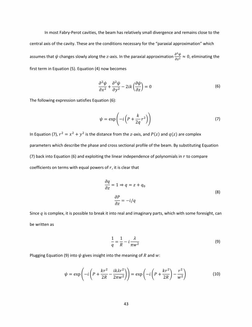
43

In most Fabry-Perot cavities, the beam has relatively small divergence and remains close to the

central axis of the cavity. These are the conditions necessary for the “paraxial approximation” which

assumes that 𝜓 changes slowly along the 𝑧-axis. In the paraxial approximation 𝜕2𝜓

𝜕𝑧2≈ 0, eliminating the

first term in Equation (5). Equation (4) now becomes

𝜕2𝜓

𝜕𝑥2+𝜕2𝜓

𝜕𝑦2− 2𝑖𝑘 (

𝜕𝜓

𝜕𝑧) = 0 (6)

The following expression satisfies Equation (6):

𝜓 = exp(−𝑖 (𝑃 +𝑘

2𝑞𝑟2)) (7)

In Equation (7), 𝑟2 = 𝑥2 + 𝑦2 is the distance from the 𝑧-axis, and 𝑃(𝑧) and 𝑞(𝑧) are complex

parameters which describe the phase and cross sectional profile of the beam. By substituting Equation

(7) back into Equation (6) and exploiting the linear independence of polynomials in 𝑟 to compare

coefficients on terms with equal powers of 𝑟, it is clear that

𝜕𝑞

𝜕𝑧= 1 ⇒ 𝑞 = 𝑧 + 𝑞0

𝜕𝑃

𝜕𝑧= −𝑖/𝑞

(8)

Since 𝑞 is complex, it is possible to break it into real and imaginary parts, which with some foresight, can

be written as

1

𝑞=1

𝑅− 𝑖

𝜆

𝜋𝑤2 (9)

Plugging Equation (9) into 𝜓 gives insight into the meaning of 𝑅 and 𝑤:

𝜓 = exp(−𝑖 (𝑃 +𝑘𝑟2

2𝑅−𝑖𝑘𝜆𝑟2

2𝜋𝑤2)) = exp (−𝑖 (𝑃 +𝑘𝑟2

2𝑅) −

𝑟2

𝑤2) (10)

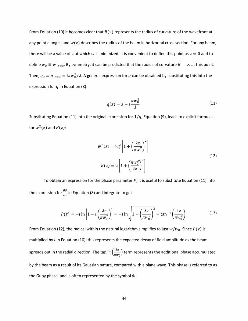
44

From Equation (10) it becomes clear that 𝑅(𝑧) represents the radius of curvature of the wavefront at

any point along 𝑧, and 𝑤(𝑧) describes the radius of the beam in horizontal cross section. For any beam,

there will be a value of 𝑧 at which 𝑤 is minimized. It is convenient to define this point as 𝑧 = 0 and to

define 𝑤0 ≡ 𝑤|𝑧=0. By symmetry, it can be predicted that the radius of curvature 𝑅 = ∞ at this point.

Then, 𝑞0 ≡ 𝑞|𝑧=0 = 𝑖𝜋𝑤02 𝜆⁄ . A general expression for 𝑞 can be obtained by substituting this into the

expression for 𝑞 in Equation (8):

𝑞(𝑧) = 𝑧 + 𝑖𝜋𝑤0

2

𝜆 (11)

Substituting Equation (11) into the original expression for 1/𝑞, Equation (9), leads to explicit formulas

for 𝑤2(𝑧) and 𝑅(𝑧):

𝑤2(𝑧) = 𝑤02 [1 + (

𝜆𝑧

𝜋𝑤02)

2

]

𝑅(𝑧) = 𝑧 [1 + (𝜋𝑤0

2

𝜆𝑧)

2

]

(12)

To obtain an expression for the phase parameter 𝑃, it is useful to substitute Equation (11) into

the expression for 𝜕𝑃

𝜕𝑧 in Equation (8) and integrate to get

𝑃(𝑧) = −𝑖 ln [1 − 𝑖 (𝜆𝑧

𝜋𝑤02)] = −𝑖 ln√1 + (

𝜆𝑧

𝜋𝑤02)

2

− tan−1 (𝜆𝑧

𝜋𝑤02) (13)

From Equation (12), the radical within the natural logarithm simplifies to just 𝑤/𝑤0. Since 𝑃(𝑧) is

multiplied by 𝑖 in Equation (10), this represents the expected decay of field amplitude as the beam

spreads out in the radial direction. The tan−1 (𝜆𝑧

𝜋𝑤02) term represents the additional phase accumulated

by the beam as a result of its Gaussian nature, compared with a plane wave. This phase is referred to as

the Guoy phase, and is often represented by the symbol Φ.

45

The final expression for the field is therefore:

𝑢(𝑟, 𝑧) =𝑤0𝑤exp [−𝑖(𝑘𝑧 − Φ) − 𝑟2 (

1

𝑤2+𝑖𝑘

2𝑅)] (14)

Careful observation of the scalar wave equation and the solution found above reveals that Equation (14)

is actually a special case of a more general form. Starting with Equation (7), one might postulate that a

more general solution would be of the form:

𝜓 = 𝑔 (𝑥

𝑤)ℎ (

𝑦

𝑤) exp(−𝑖 (𝑃 +

𝑘

2𝑞𝑟2)) (15)

By substituting this trial solution into the wave equation, it becomes clear that the wave equation is

satisfied when 𝑔 (𝑥

𝑤) and ℎ (

𝑦

𝑤) are Hermite polynomials. Equation (7) is simply the special case of this

expression for which 𝑔 (𝑥

𝑤) = ℎ (

𝑦

𝑤) = 1, which is the zeroth order Hermite polynomial. Higher-order

Hermite polynomials produce solutions with different transverse spatial profiles. Mode numbers 𝑛 and

𝑚 specify the order of the Hermite polynomial used to describe the field in the 𝑥 and 𝑦 directions

respectively. The Guoy phase, is also modified for the higher-order modes:

Φ = (1 +𝑚 + 𝑛)arctan(𝜆𝑧

𝜋𝑤02) (16)

The final expression for all of the modes (within the paraxial approximation) is therefore:

𝑢(𝑥, 𝑦, 𝑧,𝑚, 𝑛) = 𝐻𝑛 (√2𝑥

𝑤)𝐻𝑚 (

√2𝑦

𝑤)𝑤0𝑤exp [−𝑖(𝑘𝑧 − 𝛷) − 𝑟2 (

1

𝑤2+𝑖𝑘

2𝑅)] (17)

The transverse spatial profiles of several of these modes are shown in Figure 7 below.

46

Figure 7: Transverse spatial mode profiles of the first 9 Hermite Gauss optical cavity modes.

2. Hermite Gauss Modes in a Fabry-Perot Cavity

The derivation of the Hermite Gauss modes so far has assumed free-space boundary conditions.

For a mode to be stable within a Fabry-Perot cavity, it is required that the mode remain self-consistent

after one complete round trip through the cavity. This has a few logical implications: (1) the phase fronts

of the beam must be parallel to the surfaces of the mirror, such that light incident on the mirrors

retraces its path upon reflection, and (2) the total phase change between one mirror and the next must

be an integer multiple of 𝜋 so that destructive interference does not occur when beams reflect back and

47

forth many times. For a perfectly symmetrical system of two concave mirrors with radius of curvature

𝑅mirror a distance 𝐿 apart, the first of these can be expressed mathematically 𝑅 (𝐿

2) = 𝑅mirror.

Substituting this into Equation (12) yields 𝑅mirror = (𝐿

2) [1 + (

𝜋𝑤02

𝜆(𝐿 2⁄ ))2

], which can be solved for the

beam waist 𝑤0.

The second implication can be expressed as 𝑘𝑧 − 2Φ = 𝑛int𝜋, where 𝑛int represents an

arbitrary integer. From the second implication it is possible to derive a formula for the resonant

frequency of the optical modes:

𝜈

FSR= (𝑛int + 1) +

1

𝜋(𝑚 + 𝑛 + 1) arccos (1 −

𝐿

𝑅mirror) (18)

In Equation (18), 𝜈 is the frequency of the optical mode and FSR ≡ 𝑐/2𝐿 is the free spectral range of the

optical cavity. From Equation (18), it is clear that except for special cases where the second term

produces integers, higher-order modes of different total mode number 𝑚+ 𝑛 are in general non-

degenerate in frequency with each other. Therefore, to couple light into an optical cavity, the light must

match both the spatial profile and frequency of a mode as defined by the cavity mirrors. In the

experiments described in the forthcoming chapters, since light from the lasers is typically in a free-space

fundamental Gaussian mode (𝑛 = 𝑚 = 0), the light typically couples most strongly to the

corresponding mode in our optical cavities. However, precisely matching the beam shape and

convergence angle to the fundamental Gaussian mode defined by the cavity mirrors is technically

challenging, and therefore the spatial profile of the incident beam always has some overlap with the

higher-order modes. Thus, changing laser frequency alone is generally sufficient to drive higher-order

Hermite-Gauss modes, albeit at reduced efficiency.

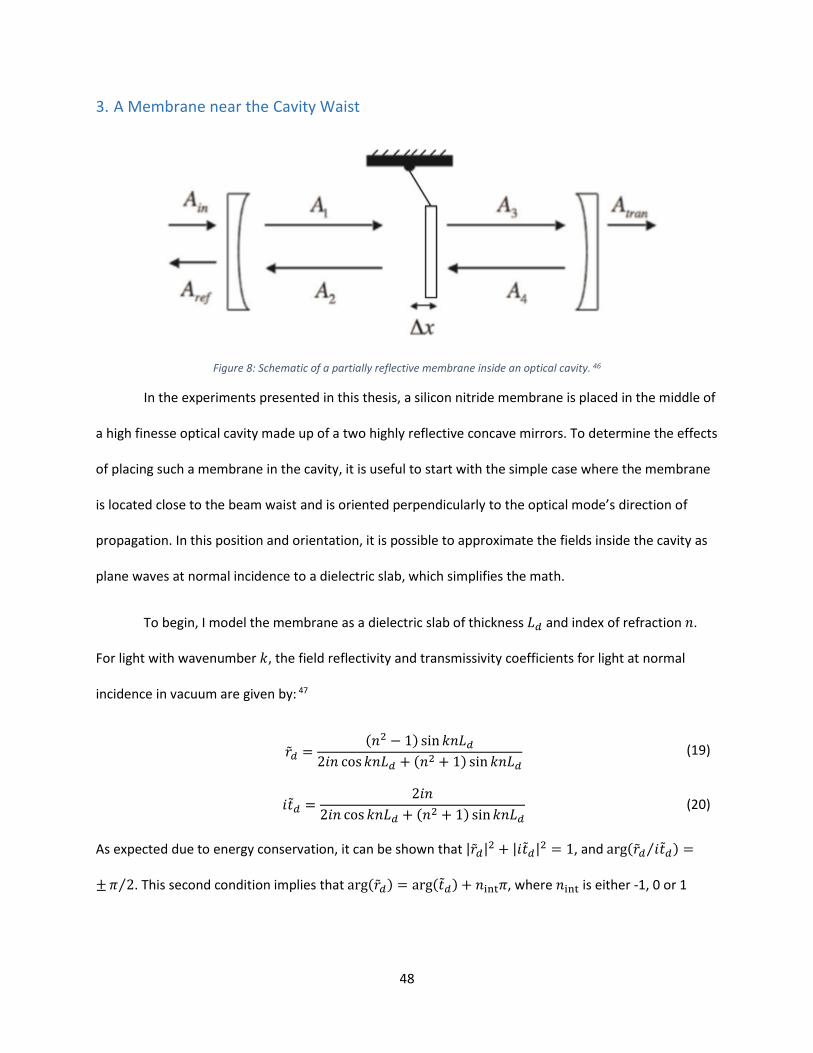
48

3. A Membrane near the Cavity Waist

Figure 8: Schematic of a partially reflective membrane inside an optical cavity. 46

In the experiments presented in this thesis, a silicon nitride membrane is placed in the middle of

a high finesse optical cavity made up of a two highly reflective concave mirrors. To determine the effects

of placing such a membrane in the cavity, it is useful to start with the simple case where the membrane

is located close to the beam waist and is oriented perpendicularly to the optical mode’s direction of

propagation. In this position and orientation, it is possible to approximate the fields inside the cavity as

plane waves at normal incidence to a dielectric slab, which simplifies the math.

To begin, I model the membrane as a dielectric slab of thickness 𝐿𝑑 and index of refraction 𝑛.

For light with wavenumber 𝑘, the field reflectivity and transmissivity coefficients for light at normal

incidence in vacuum are given by: 47

��𝑑 =(𝑛2 − 1) sin 𝑘𝑛𝐿𝑑

2𝑖𝑛 cos𝑘𝑛𝐿𝑑 + (𝑛2 + 1) sin 𝑘𝑛𝐿𝑑

(19)

𝑖��𝑑 =2𝑖𝑛

2𝑖𝑛 cos 𝑘𝑛𝐿𝑑 + (𝑛2 + 1) sin𝑘𝑛𝐿𝑑

(20)

As expected due to energy conservation, it can be shown that |��𝑑|2 + |𝑖��𝑑|

2 = 1, and arg(��𝑑 𝑖��𝑑⁄ ) =

±𝜋 2⁄ . This second condition implies that arg(��𝑑) = arg(��𝑑) + 𝑛int𝜋, where 𝑛int is either -1, 0 or 1

49

depending on the values of 𝑘, 𝐿𝑑, and 𝑛. In the limit 𝐿𝑑 ≪ 𝜆 with realistic index of refraction 𝑛 ≈ 2, it

can be shown that the complex phases of ��𝑑 and ��𝑑 are equal, which is important later.

With 𝑟1 (𝑖𝑡1) and 𝑟2 (𝑖𝑡2) representing the field reflectivity (transmissivity) of mirrors 1 and 2

respectively, the system of equations describing the field amplitudes within the system is:

𝐴1 = 𝑖𝑡1𝐴in + 𝑟1𝐴2𝑒𝑖𝑘𝐿1

𝐴2 = ��𝑑𝐴1𝑒𝑖𝑘𝐿1 + 𝑖��𝑑𝐴4𝑒

𝑖𝑘𝐿2

𝐴3 = 𝑖��𝑑𝐴1𝑒𝑖𝑘𝐿1 + ��𝑑𝐴4𝑒

𝑖𝑘𝐿2

𝐴4 = 𝑟2𝐴3𝑒𝑖𝑘𝐿2

𝐴refl = 𝑖𝑡1𝐴2𝑒𝑖𝑘𝐿1 + 𝑟1𝐴in

𝐴tran = 𝑖𝑡2𝐴3𝑒𝑖𝑘𝐿2

(21)

As a system of six equations with six unknowns, it is possible to obtain analytic expressions for

each field component. However, this is unnecessarily complicated and yields unwieldy equations. In

practice, what we care about is the just the frequency of the cavity eigenmodes as a function of

membrane position, i.e. we want to find combinations of 𝑘, 𝐿1, and 𝐿2 that provide non-trivial solutions

to the system of equations. Since this depends only on the fields and boundary conditions within the

cavity and is independent of the presence of any laser drive, we can neglect the equations for 𝐴refl and

𝐴tran and set 𝐴in → 0. We also, for clarity, shall write out explicitly the complex phases of ��𝑑 and ��𝑑 as

��𝑑 = 𝑟𝑑𝑒𝑖𝜙 and ��𝑑 = 𝑡𝑑𝑒

𝑖𝜙 so that it is easier to follow them through the computation. We can then

write the system of equations in matrix form as follows:

(

𝐴1𝐴2𝐴3𝐴4

) =

[

0 𝑟1𝑒𝑖𝑘𝐿1 0 0

𝑟𝑑𝑒𝑖𝑘𝐿1+𝑖𝜙 0 0 𝑖𝑡𝑑𝑒

𝑖𝑘𝐿2+𝑖𝜙

𝑖𝑡𝑑𝑒𝑖𝑘𝐿1+𝑖𝜙 0 0 𝑟𝑑𝑒

𝑖𝑘𝐿2+𝑖𝜙

0 0 𝑟2𝑒𝑖𝑘𝐿2 0 ]

(

𝐴1𝐴2𝐴3𝐴4

) (22)

The four eigenvalues of this matrix are:

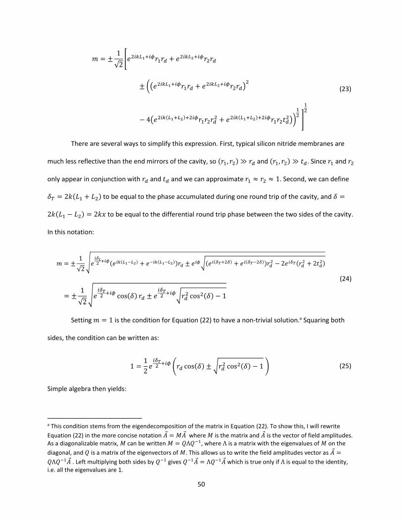
50

𝑚 = ±1

√2[𝑒2𝑖𝑘𝐿1+𝑖𝜙𝑟1𝑟𝑑 + 𝑒

2𝑖𝑘𝐿2+𝑖𝜙𝑟2𝑟𝑑

± ((𝑒2𝑖𝑘𝐿1+𝑖𝜙𝑟1𝑟𝑑 + 𝑒2𝑖𝑘𝐿2+𝑖𝜙𝑟2𝑟𝑑)

2

− 4(𝑒2𝑖𝑘(𝐿1+𝐿2)+2𝑖𝜙𝑟1𝑟2𝑟𝑑2 + 𝑒2𝑖𝑘(𝐿1+𝐿2)+2𝑖𝜙𝑟1𝑟2𝑡𝑑

2))

12 ]

12

(23)

There are several ways to simplify this expression. First, typical silicon nitride membranes are

much less reflective than the end mirrors of the cavity, so (𝑟1, 𝑟2) ≫ 𝑟𝑑 and (𝑟1, 𝑟2) ≫ 𝑡𝑑. Since 𝑟1 and 𝑟2

only appear in conjunction with 𝑟𝑑 and 𝑡𝑑 and we can approximate 𝑟1 ≈ 𝑟2 ≈ 1. Second, we can define

𝛿𝑇 = 2𝑘(𝐿1 + 𝐿2) to be equal to the phase accumulated during one round trip of the cavity, and 𝛿 =

2𝑘(𝐿1 − 𝐿2) = 2𝑘𝑥 to be equal to the differential round trip phase between the two sides of the cavity.

In this notation:

𝑚 = ±1

√2√𝑒

𝑖𝛿𝑡2+𝑖𝜙(𝑒𝑖𝑘(𝐿1−𝐿2) + 𝑒−𝑖𝑘(𝐿1−𝐿2))𝑟𝑑 ± 𝑒

𝑖𝜙√(𝑒𝑖(𝛿𝑇+2𝛿) + 𝑒𝑖(𝛿𝑇−2𝛿))𝑟𝑑2 − 2𝑒𝑖𝛿𝑇(𝑟𝑑

2 + 2𝑡𝑑2)

= ±1

√2√𝑒

𝑖𝛿𝑇2+𝑖𝜙 cos(𝛿) 𝑟𝑑 ± 𝑒

𝑖𝛿𝑇2+𝑖𝜙√𝑟𝑑

2 cos2(𝛿) − 1

(24)

Setting 𝑚 = 1 is the condition for Equation (22) to have a non-trivial solution.a Squaring both

sides, the condition can be written as:

1 =1

2𝑒𝑖𝛿𝑇2+𝑖𝜙 (𝑟𝑑 cos(𝛿) ± √𝑟𝑑

2 cos2(𝛿) − 1 ) (25)

Simple algebra then yields:

a This condition stems from the eigendecomposition of the matrix in Equation (22). To show this, I will rewrite

Equation (22) in the more concise notation 𝐴 = 𝑀𝐴 where 𝑀 is the matrix and 𝐴 is the vector of field amplitudes. As a diagonalizable matrix, 𝑀 can be written 𝑀 = 𝑄Λ𝑄−1, where Λ is a matrix with the eigenvalues of 𝑀 on the

diagonal, and 𝑄 is a matrix of the eigenvectors of 𝑀. This allows us to write the field amplitudes vector as 𝐴 =

𝑄Λ𝑄−1𝐴 . Left multiplying both sides by 𝑄−1 gives 𝑄−1𝐴 = Λ𝑄−1𝐴 which is true only if Λ is equal to the identity, i.e. all the eigenvalues are 1.

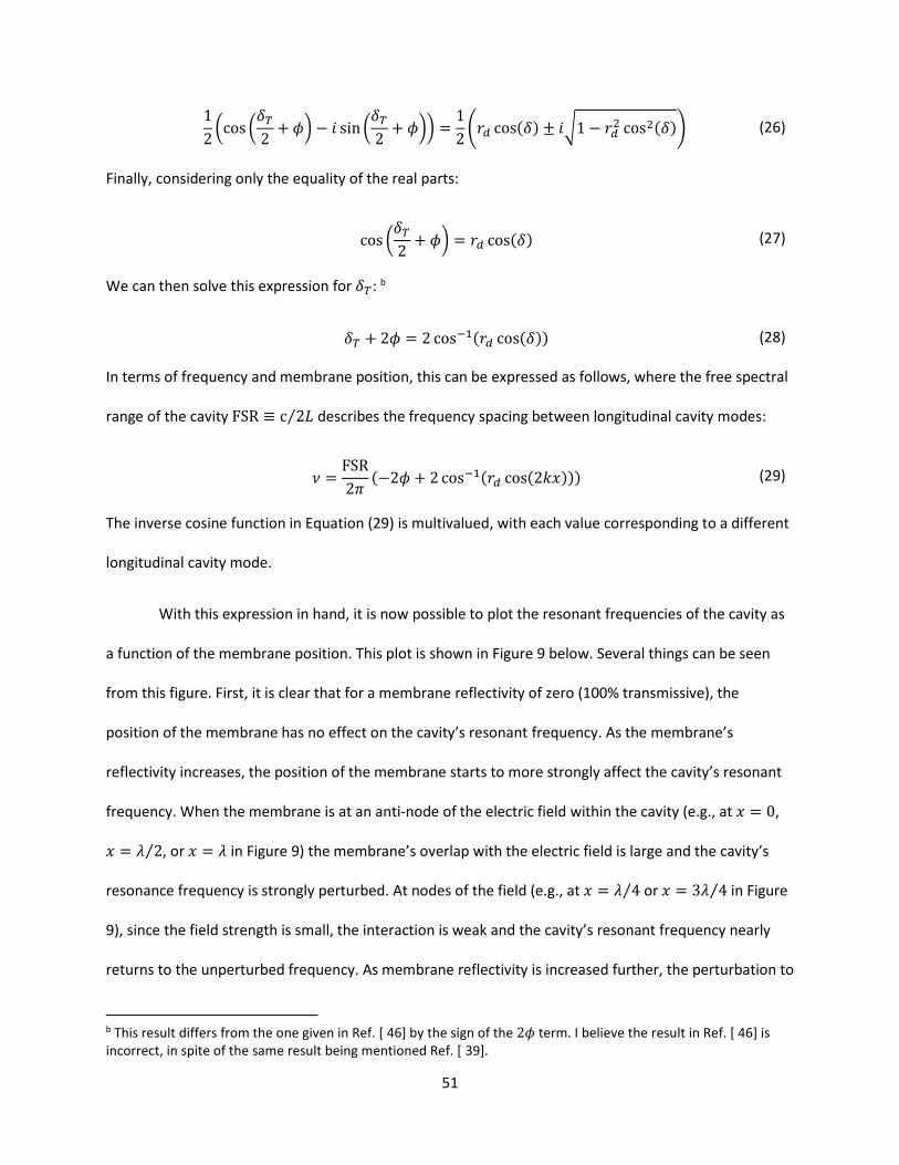
51

1

2(cos (

𝛿𝑇2+ 𝜙) − 𝑖 sin (

𝛿𝑇2+ 𝜙)) =

1

2(𝑟𝑑 cos(𝛿) ± 𝑖√1 − 𝑟𝑑

2 cos2(𝛿)) (26)

Finally, considering only the equality of the real parts:

cos (𝛿𝑇2+ 𝜙) = 𝑟𝑑 cos(𝛿) (27)

We can then solve this expression for 𝛿𝑇: b

𝛿𝑇 + 2𝜙 = 2 cos−1(𝑟𝑑 cos(𝛿)) (28)

In terms of frequency and membrane position, this can be expressed as follows, where the free spectral

range of the cavity FSR ≡ c 2𝐿⁄ describes the frequency spacing between longitudinal cavity modes:

𝜈 =FSR

2𝜋(−2𝜙 + 2 cos−1(𝑟𝑑 cos(2𝑘𝑥))) (29)

The inverse cosine function in Equation (29) is multivalued, with each value corresponding to a different

longitudinal cavity mode.

With this expression in hand, it is now possible to plot the resonant frequencies of the cavity as

a function of the membrane position. This plot is shown in Figure 9 below. Several things can be seen

from this figure. First, it is clear that for a membrane reflectivity of zero (100% transmissive), the

position of the membrane has no effect on the cavity’s resonant frequency. As the membrane’s

reflectivity increases, the position of the membrane starts to more strongly affect the cavity’s resonant

frequency. When the membrane is at an anti-node of the electric field within the cavity (e.g., at 𝑥 = 0,

𝑥 = 𝜆 2⁄ , or 𝑥 = 𝜆 in Figure 9) the membrane’s overlap with the electric field is large and the cavity’s

resonance frequency is strongly perturbed. At nodes of the field (e.g., at 𝑥 = 𝜆 4⁄ or 𝑥 = 3𝜆 4⁄ in Figure

9), since the field strength is small, the interaction is weak and the cavity’s resonant frequency nearly

returns to the unperturbed frequency. As membrane reflectivity is increased further, the perturbation to

b This result differs from the one given in Ref. [ 46] by the sign of the 2𝜙 term. I believe the result in Ref. [ 46] is incorrect, in spite of the same result being mentioned Ref. [ 39].

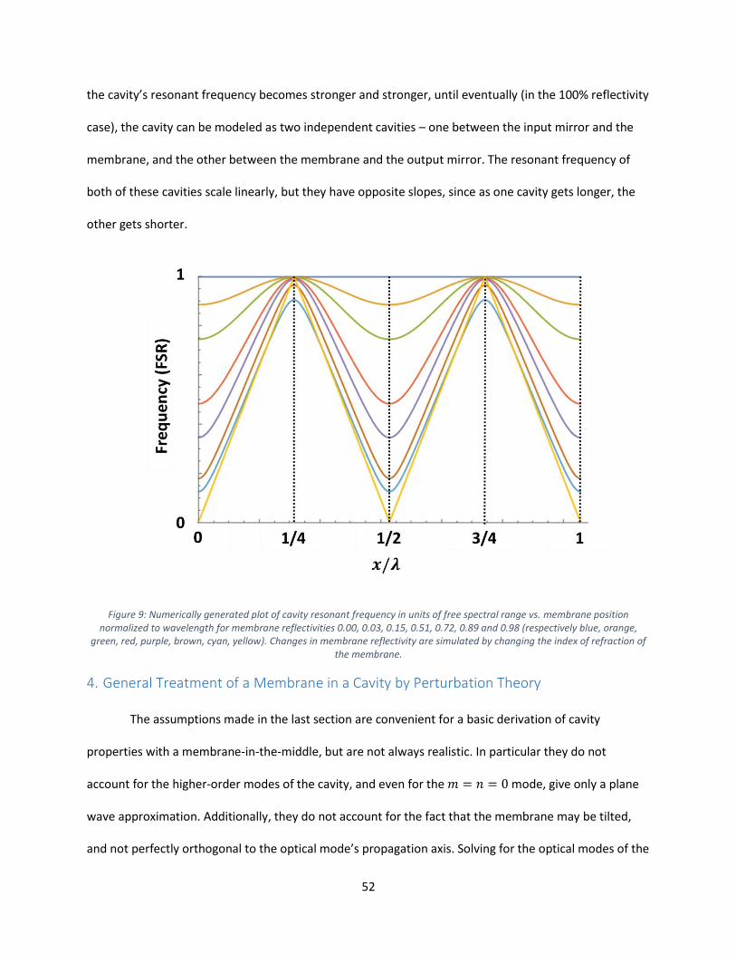
52

the cavity’s resonant frequency becomes stronger and stronger, until eventually (in the 100% reflectivity

case), the cavity can be modeled as two independent cavities – one between the input mirror and the

membrane, and the other between the membrane and the output mirror. The resonant frequency of

both of these cavities scale linearly, but they have opposite slopes, since as one cavity gets longer, the

other gets shorter.

Figure 9: Numerically generated plot of cavity resonant frequency in units of free spectral range vs. membrane position normalized to wavelength for membrane reflectivities 0.00, 0.03, 0.15, 0.51, 0.72, 0.89 and 0.98 (respectively blue, orange,

green, red, purple, brown, cyan, yellow). Changes in membrane reflectivity are simulated by changing the index of refraction of the membrane.

4. General Treatment of a Membrane in a Cavity by Perturbation Theory

The assumptions made in the last section are convenient for a basic derivation of cavity

properties with a membrane-in-the-middle, but are not always realistic. In particular they do not

account for the higher-order modes of the cavity, and even for the 𝑚 = 𝑛 = 0 mode, give only a plane

wave approximation. Additionally, they do not account for the fact that the membrane may be tilted,

and not perfectly orthogonal to the optical mode’s propagation axis. Solving for the optical modes of the

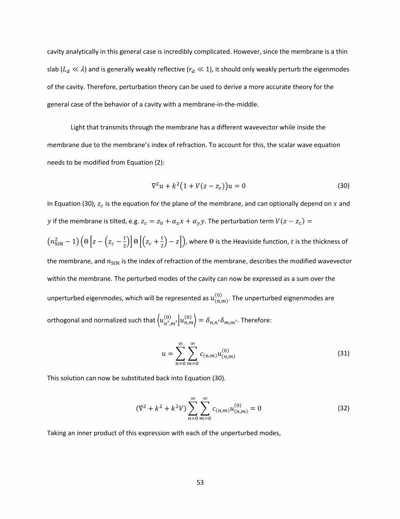
53

cavity analytically in this general case is incredibly complicated. However, since the membrane is a thin

slab (𝐿𝑑 ≪ 𝜆) and is generally weakly reflective (𝑟𝑑 ≪ 1), it should only weakly perturb the eigenmodes

of the cavity. Therefore, perturbation theory can be used to derive a more accurate theory for the

general case of the behavior of a cavity with a membrane-in-the-middle.

Light that transmits through the membrane has a different wavevector while inside the

membrane due to the membrane’s index of refraction. To account for this, the scalar wave equation

needs to be modified from Equation (2):

∇2𝑢 + 𝑘2(1 + 𝑉(𝑧 − 𝑧𝑐))𝑢 = 0 (30)

In Equation (30), 𝑧𝑐 is the equation for the plane of the membrane, and can optionally depend on 𝑥 and

𝑦 if the membrane is tilted, e.g. 𝑧𝑐 = 𝑧0 + 𝛼𝑥𝑥 + 𝛼𝑦𝑦. The perturbation term 𝑉(𝑧 − 𝑧𝑐) =

(𝑛SiN2 − 1) (Θ [𝑧 − (𝑧𝑐 −

𝑡

2)]Θ [(𝑧𝑐 +

𝑡

2) − 𝑧]), where Θ is the Heaviside function, 𝑡 is the thickness of

the membrane, and 𝑛SiN is the index of refraction of the membrane, describes the modified wavevector

within the membrane. The perturbed modes of the cavity can now be expressed as a sum over the

unperturbed eigenmodes, which will be represented as 𝑢(𝑛,𝑚)(0)

. The unperturbed eignenmodes are

orthogonal and normalized such that ⟨𝑢𝑛′,𝑚′(0)

|𝑢𝑛,𝑚(0)⟩ = 𝛿𝑛,𝑛′𝛿𝑚,𝑚′. Therefore:

𝑢 = ∑ ∑ 𝑐(𝑛,𝑚)𝑢(𝑛,𝑚)(0)

∞

𝑚=0

∞

𝑛=0

(31)

This solution can now be substituted back into Equation (30).

(∇2 + 𝑘2 + 𝑘2𝑉)∑ ∑ 𝑐(𝑛,𝑚)𝑢(𝑛,𝑚)(0)

∞

𝑚=0

∞

𝑛=0

= 0 (32)

Taking an inner product of this expression with each of the unperturbed modes,

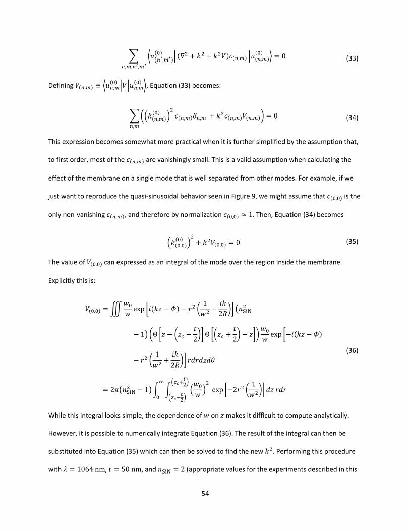
54

∑ ⟨𝑢(𝑛′,𝑚′)

(0)| (∇2 + 𝑘2 + 𝑘2𝑉)𝑐(𝑛,𝑚) |𝑢(𝑛,𝑚)

(0)⟩

𝑛,𝑚,𝑛′,𝑚′

= 0 (33)

Defining 𝑉(𝑛,𝑚) ≡ ⟨𝑢𝑛,𝑚(0)|𝑉|𝑢𝑛,𝑚

(0)⟩, Equation (33) becomes:

∑((𝑘(𝑛,𝑚)(0) )

2𝑐(𝑛,𝑚)𝛿𝑛,𝑚 + 𝑘

2𝑐(𝑛,𝑚)𝑉(𝑛,𝑚))

𝑛,𝑚

= 0 (34)

This expression becomes somewhat more practical when it is further simplified by the assumption that,

to first order, most of the 𝑐(𝑛,𝑚) are vanishingly small. This is a valid assumption when calculating the

effect of the membrane on a single mode that is well separated from other modes. For example, if we

just want to reproduce the quasi-sinusoidal behavior seen in Figure 9, we might assume that 𝑐(0,0) is the

only non-vanishing 𝑐(𝑛,𝑚), and therefore by normalization 𝑐(0,0) ≈ 1. Then, Equation (34) becomes

(𝑘(0,0)(0) )

2+ 𝑘2𝑉(0,0) = 0 (35)

The value of 𝑉(0,0) can expressed as an integral of the mode over the region inside the membrane.

Explicitly this is:

𝑉(0,0) =∭𝑤0𝑤exp [𝑖(𝑘𝑧 − 𝛷) − 𝑟2 (

1

𝑤2−𝑖𝑘

2𝑅)] (𝑛SiN

2

− 1) (Θ [𝑧 − (𝑧𝑐 −𝑡

2)]Θ [(𝑧𝑐 +

𝑡

2) − 𝑧])

𝑤0𝑤exp [−𝑖(𝑘𝑧 − 𝛷)

− 𝑟2 (1

𝑤2+𝑖𝑘

2𝑅)] 𝑟𝑑𝑟𝑑𝑧𝑑𝜃

= 2𝜋(𝑛SiN2 − 1)∫ ∫ (

𝑤0𝑤)2

exp [−2𝑟2 (1

𝑤2)] 𝑑𝑧

(𝑧𝑐+𝑡2)

(𝑧𝑐−𝑡2)

𝑟𝑑𝑟∞

0

(36)

While this integral looks simple, the dependence of 𝑤 on 𝑧 makes it difficult to compute analytically.

However, it is possible to numerically integrate Equation (36). The result of the integral can then be

substituted into Equation (35) which can then be solved to find the new 𝑘2. Performing this procedure

with 𝜆 = 1064 nm, 𝑡 = 50 nm, and 𝑛SiN = 2 (appropriate values for the experiments described in this

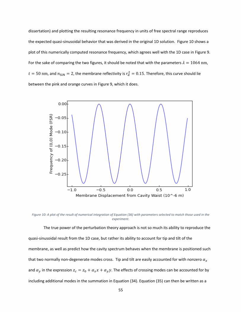
55

dissertation) and plotting the resulting resonance frequency in units of free spectral range reproduces

the expected quasi-sinusoidal behavior that was derived in the original 1D solution. Figure 10 shows a

plot of this numerically computed resonance frequency, which agrees well with the 1D case in Figure 9.

For the sake of comparing the two figures, it should be noted that with the parameters 𝜆 = 1064 nm,

𝑡 = 50 nm, and 𝑛SiN = 2, the membrane reflectivity is 𝑟𝑑2 = 0.15. Therefore, this curve should lie

between the pink and orange curves in Figure 9, which it does.

Figure 10: A plot of the result of numerical integration of Equation (36) with parameters selected to match those used in the experiment.

The true power of the perturbation theory approach is not so much its ability to reproduce the

quasi-sinusoidal result from the 1D case, but rather its ability to account for tip and tilt of the

membrane, as well as predict how the cavity spectrum behaves when the membrane is positioned such

that two normally non-degenerate modes cross. Tip and tilt are easily accounted for with nonzero 𝛼𝑥

and 𝛼𝑦 in the expression 𝑧𝑐 = 𝑧0 + 𝛼𝑥𝑥 + 𝛼𝑦𝑦. The effects of crossing modes can be accounted for by

including additional modes in the summation in Equation (34). Equation (35) can then be written as a

56

matrix equation, and the integrals for each 𝑉(𝑛,𝑚) computed numerically. Solving for the eigenvalues of

the matrix yields the perturbed cavity resonance frequencies. Figure 11 shows an example of the

interaction between the three triplet modes (TEM0,2, TEM1,1, and TEM2,0) of one longitudinal mode and

the fundamental transverse mode of the next longitudinal mode.

Figure 11: A plot of the frequencies of the (0,0), (0,2), (1,1), and (2,0) transverse modes of the optical cavity for a membrane of thickness 𝑡 = 50 𝑛𝑚 and a membrane tilt of ~0.29° along both the x and y axes. Plot is based on numerical computation of the

𝑉(𝑛,𝑚) integrals as described in the text.

Qualitatively, it is apparent that as the modes cross each other, they actually avoid becoming

fully degenerate. This is due to the reduced symmetry of the cavity in the presence of membrane tilt. As

a consequence of the modes avoiding each other, there are points in the cavity spectrum for which a

Taylor expansion of the mode frequency as a function of membrane position has no first-order term. At

these points, the cavity responds quadratically to membrane position, which can yield interesting

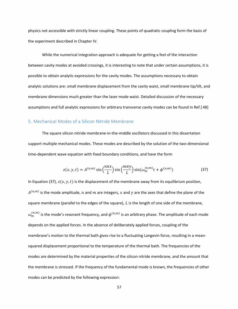
57

physics not accessible with strictly linear coupling. These points of quadratic coupling form the basis of

the experiment described in Chapter IV.

While the numerical integration approach is adequate for getting a feel of the interaction

between cavity modes at avoided crossings, it is interesting to note that under certain assumptions, it is

possible to obtain analytic expressions for the cavity modes. The assumptions necessary to obtain

analytic solutions are: small membrane displacement from the cavity waist, small membrane tip/tilt, and

membrane dimensions much greater than the laser mode waist. Detailed discussion of the necessary

assumptions and full analytic expressions for arbitrary transverse cavity modes can be found in Ref.[ 48]

5. Mechanical Modes of a Silicon Nitride Membrane

The square silicon nitride membrane-in-the-middle oscillators discussed in this dissertation

support multiple mechanical modes. These modes are described by the solution of the two-dimensional

time-dependent wave equation with fixed boundary conditions, and have the form

𝑧(𝑥, 𝑦, 𝑡) = 𝐴(𝑛,𝑚) sin (𝑛𝜋𝑥

𝐿) sin (

𝑚𝜋𝑦

𝐿) sin (𝜔𝑚

(𝑛,𝑚)𝑡 + 𝜙(𝑛,𝑚)) (37)

In Equation (37), 𝑧(𝑥, 𝑦, 𝑡) is the displacement of the membrane away from its equilibrium position,

𝐴(𝑛,𝑚) is the mode amplitude, 𝑛 and 𝑚 are integers, 𝑥 and 𝑦 are the axes that define the plane of the

square membrane (parallel to the edges of the square), 𝐿 is the length of one side of the membrane,

𝜔𝑚(𝑛,𝑚)

is the mode’s resonant frequency, and 𝜙(𝑛,𝑚) is an arbitrary phase. The amplitude of each mode

depends on the applied forces. In the absence of deliberately applied forces, coupling of the

membrane’s motion to the thermal bath gives rise to a fluctuating Langevin force, resulting in a mean-

squared displacement proportional to the temperature of the thermal bath. The frequencies of the

modes are determined by the material properties of the silicon nitride membrane, and the amount that

the membrane is stressed. If the frequency of the fundamental mode is known, the frequencies of other

modes can be predicted by the following expression:

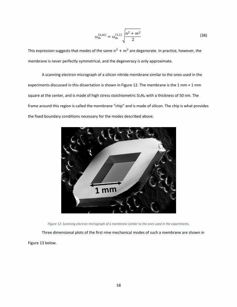
58

𝜔𝑚(𝑛,𝑚)

= 𝜔𝑚(1,1)√

𝑛2 +𝑚2

2 (38)

This expression suggests that modes of the same 𝑛2 +𝑚2 are degenerate. In practice, however, the

membrane is never perfectly symmetrical, and the degeneracy is only approximate.

A scanning electron micrograph of a silicon nitride membrane similar to the ones used in the

experiments discussed in this dissertation is shown in Figure 12. The membrane is the 1 mm × 1 mm

square at the center, and is made of high stress stoichiometric Si3N4 with a thickness of 50 nm. The

frame around this region is called the membrane “chip” and is made of silicon. The chip is what provides

the fixed boundary conditions necessary for the modes described above.

Figure 12: Scanning electron micrograph of a membrane similar to the ones used in the experiments.

Three dimensional plots of the first nine mechanical modes of such a membrane are shown in

Figure 13 below.

59

Figure 13: 3D plots of the first nine mechanical modes of a square membrane.

6. The Optomechanical Hamiltonian

The optomechanical interaction between a single membrane mechanical mode and a single

cavity optical mode is governed by a Hamiltonian that includes terms for total energy of the mechanical

and optical modes. In the simplest case, this is:

𝐻 = ℏ𝜔𝑐(𝑥)��†�� + ℏ𝜔𝑚��

†�� (39)

In this expression, �� is the optical mode photon annihilation operator, �� is the mechanical mode phonon

annihiliation operator, and 𝜔𝑚 is the mechanical mode frequency. 𝜔𝑐(��) is the resonant frequency of

the optical cavity, which as shown in Figure 6, is a function of the membrane position. The

dimensionless membrane position 𝑥 = (��† + ��). To effectively describe the coupling between the

60

mechanical and optical modes, it is useful to expand 𝜔𝑐(𝑥) in a Taylor series. For a membrane near an

arbitrary position within the cavity:

𝜔𝑐(𝑥) ≈ 𝜔𝑐 +𝜔𝑐′𝑥zpf�� +

1

2𝜔𝑐′′𝑥zpf

2 𝑥2 +⋯ (40)

where 𝜔𝑐, 𝜔𝑐′ , and 𝜔𝑐

′′ represent derivatives of 𝜔𝑐(𝑥) evaluated at the position of the membrane, and

𝑥zpf ≡ √ℏ

2𝑚𝜔𝑚 is the magnitude of the zero-point fluctuations of the mechanical mode.

Depending on the position of the membrane within the cavity, certain terms of this Taylor

expansion may be more or less important. For example, as seen in Figure 6, in between nodes and

antinodes of the intracavity field, the cavity detuning as a function of membrane position is

predominantly linear, and 𝜔𝑐(𝑥) ≈ 𝜔𝑐 +𝜔𝑐′𝑥zpf��. At points such as these, the coupling between the

mechanical and optical modes is said to be “linear,” and its strength is characterized by the linear

optomechanical coupling parameter: 𝑔 ≡ 𝜔𝑐′𝑥zpf. At the node or antinode however, the linear term of

the Taylor expansion vanishes, and the second-order term of the Taylor expansion becomes significant,

𝜔𝑐(𝑥) ≈ 𝜔𝑐 +1

2𝜔𝑐′′𝑥zpf

2 𝑥2. In this case, the optomechanical coupling is said to be quadratic, and the

strength of the coupling is characterized by the quadratic optomechanical coupling parameter 𝑔2 ≡

𝜔𝑐′′𝑥zpf

2 .

Therefore, changing the position of the membrane within the cavity changes both the strength

and functional form of the coupling between the mechanical oscillator and the cavity’s resonant

frequency. 37 Avoided crossings between cavity modes, as described above, can produce points that

exhibit much stronger quadratic coupling than can be obtained at nodes and antinodes of the intracavity

field, permitting exploration of a range of new physical effects. 43, 49

In this dissertation I will describe two experiments. The first involves the use of a point of linear

coupling to demonstrate near ground state cooling of one mechanical mode of the membrane. The

61

second involves the use of a point of quadratic coupling formed by the avoided crossing between two

cavity modes to explore the classical dynamics of the quadratic optomechanical interaction. I shall

discuss the details of how the optomechanical Hamiltonian leads to the observed effects in each case in

the Theory section of each of following chapters.

62

III. Ground State Cooling

As discussed in the introduction, cooling a mechanical oscillator to its vibrational ground state is

a useful first step in preparing the oscillator to store an arbitrary quantum state. Additionally, cooling an

oscillator to the ground state reduces the thermal contribution to the spectrum of the oscillator’s

motion, which can enhance the visibility of radiation pressure shot noise. Furthermore, the smaller

thermal contribution to the oscillator’s motion may, with an appropriate measurement, allow for

observation of quantum jumps between phonon levels.

The term “ground state cooling” refers to cooling one or more of the membrane’s mechanical

modes until the phonon occupancy of the mode or modes is close to zero, i.e. the amplitude of motion

is close to the zero-point fluctuations of the mode as predicted by quantum mechanics: 𝐴(𝑛,𝑚) ≈ 𝑥zpf ≡

√ℏ

2𝑚𝜔𝑚. If cooling is done by lowering the temperature of the thermal bath (such as by placing the

system inside a cryostat), then by the classical equipartition theorem, all of the modes will be cooled to

a phonon occupancy of 𝑛𝑚(𝑛,𝑚) = 𝑘B𝑇 ℏ𝜔𝑚

(𝑛,𝑚)⁄ . However, as discussed in the introduction, cryogenic

cooling is generally insufficient to cool low-frequency modes of massive mechanical oscillators to their

ground states. Sideband cooling of the sort discussed in the introduction does not generally cool all

modes by the same amount. Therefore, the term “ground state cooling” in reference to systems cooled

by sideband cooling generally refers to efforts targeted at cooling only one mechanical mode of the

oscillator.

Though ground state cooling has previously been achieved in many optomechanical systems, 5, 6,

7, 8, 9, 10 it is still a goal worth pursuing in the membrane-in-the-middle system. First, the membrane

cooled in the experiment described in this dissertation has an effective mass on the order of tens of

nanograms, and dimensions on the order of 1 mm2, making it visible to the naked eye. The mechanical

63

frequency of the mode selected for ground state cooling is less than 1 MHz. 11 These parameters put this

system among the heaviest, lowest frequency mechanical oscillators cooled to the ground state. Cooling

such a massive and low-frequency oscillator to the ground state is incredibly challenging because of the

low effective temperature that must be achieved. As discussed in the introduction, a ~MHz frequency

oscillator in its ground state has an effective temperature of approximately 50 μK, necessitating very

careful experimental design to isolate the oscillator from the comparatively “hot” cryogenic bath. Also,

classical laser noise is generally worse at ~MHz and lower frequencies, and this further confounds efforts

to cool such low-frequency oscillators.

Notwithstanding the technical accomplishments required to cool a membrane oscillator to its

ground state, the effort to achieve ground state cooling in such a system is worthwhile because it allows

for tests of the predictions of quantum mechanics in a truly macroscopic object. Additionally, a

membrane-in-the-middle system has particular advantages over many other optomechanical systems in

terms of tunability. As previously discussed, the membrane can be translated, tipped, and tilted within

the optical cavity to change the functional form of the coupling between the cavity’s resonant frequency

and the mechanical mode. By selecting appropriate points within the cavity spectrum, it is possible to

obtain linear coupling to one optical mode, and quadratic coupling to another mode, allowing for

ground state cooling while simultaneously exploring the dynamics of non-linear coupling. This flexibility

is not found in other systems, and is a major reason why ground state cooling of a membrane-in-the-

middle is valuable.

1. Theory

In this section I seek to derive the how sideband cooling of a mechanical oscillator works using a

Hamiltonian formalism. While I shall refer to the mechanical oscillator as the “membrane”, this

formalism is actually completely general, and could apply to any optomechanics experiment that uses

64

one laser to measure the motion of the mechanical oscillator, and a second laser to perform sideband

cooling. I will begin with the Hamiltonian of the membrane/cavity system, which can be written as:

𝐻 = ∑ ℏ(𝜔𝑗 + 𝑔𝑗𝑥)��𝑗†��𝑗 + ℏ𝜔𝑚��

†�� + 𝐻drive + 𝐻diss𝑗=𝑠,𝑝

(41)

In the summation over 𝑗, 𝑠 represents the optical cavity mode addressed by the measurement laser, and

𝑝 represents the mode addressed by the cooling laser. 𝜔𝑗 represents the frequency of each mode, 𝑔𝑗 =

𝜔𝑗′𝑥zpf (where 𝜔𝑗

′ is the slope of the cavity’s resonant frequency as a function of membrane position,

and 𝑥zpf = √ℏ

2𝑚𝜔𝑚 is the amplitude of the zero-point fluctuations of the membrane’s position) is the

optomechanical coupling of membrane to each optical mode mode, and ��𝑗 is the photon annihilation

operator for each mode. 𝜔𝑚 is the frequency of the membrane’s mechanical mode of interest, and �� is

the phonon annihilation operator for that mode. The membrane’s position is therefore given by 𝑥 =

𝑥𝑜 + (�� + ��†), where 𝑥0 = ⟨𝑥⟩ is the membrane’s time-averaged position (in units of the zero-point

fluctuations) which we may define to be 0. 𝐻drive and 𝐻diss respectively represent the laser drive, and

the coupling rate of both the cavity and the membrane to the outside environment.

The interaction term, ℏ𝑔𝑗𝑥��𝑗†��𝑗 describes how the membrane’s motion interacts with the

electromagnetic field inside the cavity, as well as how the electromagnetic field interacts with the

membrane. In the limit of a strong laser drive and weak coupling such that the membrane induces only

small fluctuations in the amplitude of the electromagnetic field in the cavity, the interaction term can be

linearized. In this approximation, it is simple to predict the types of interactions that can occur between

the mechanical mode and the optical cavity mode(s) by inspection of the Hamiltonian. In the linearized

approximation, the cavity field is expressed in terms of an average coherent amplitude ��𝑗 and

fluctuations ��𝑗:

65

��𝑗 = ��𝑗 + ��𝑗 (42)

Substituting this into the interaction Hamiltonian gives

𝐻int = ℏ𝑔𝑗(��𝑗 + ��𝑗)†(��𝑗 + ��𝑗)(�� + ��

†) (43)

In this expression, there are several terms. The |��𝑗|2

term indicates that there is a static force acting on

the membrane due to the average field in the cavity, which results in a constant shift in membrane’s

position. This term can therefore be removed from the expression by simply redefining 𝑥0. Terms that

are quadratic in ��𝑗 can be neglected since ��𝑗 is already small to first order. The remaining terms describe

the linear interaction between the mechanical and optical modes:

𝐻intlin = ℏ𝑔𝑗(��𝑗

∗��𝑗 + ��𝑗��𝑗†)(�� + ��†) = ℏ𝑔𝑗��𝑗(��𝑗�� + ��𝑗 ��

† + ��𝑗†�� + ��𝑗

†��†) (44)

The terms ��𝑗 ��† + ��𝑗

†�� represent an exchange of energy between optical mode photons and mechanical

mode phonons, while the ��𝑗�� + ��𝑗†��† terms represent a two-mode squeezing interaction in which the

creation/annihilation of photons in the optical mode is correlated with creation/annihilation

(respectively) of phonons in the mechanical mode. In the photon/phonon exchange processes, the ��𝑗†��

term is referred to as the anti-Stokes process, and represents the annihilation of phonons in the

membrane in exchange for the creation of blue detuned photons. This term is the origin of

optomechanical cooling and the blue sideband in the optical spectrum. The ��𝑗†�� process is referred to as

the Stokes process, and represents the creation of phonons in the membrane in exchange for a photon

from the optical beam. This term is the origin of red sideband in the optical spectrum.

The rotating wave approximation provides a means of determining which of these four

processes is expected to occur as a function of drive laser detuning from the optical cavity mode. The

rotating wave approximation is a common method used in optical physics, in which the Hamiltonian is

rewritten in a reference frame that is oscillating at the frequency of the laser drive. To apply the rotating

66

wave approximation it is first necessary to explicitly express the phase (frequency) of each operator in

the Hamiltonian, which can be accomplished by making the following substitutions: the photon

annihilation operator can be rewritten as ��𝑗 → ��𝑗𝑒𝑖𝜔𝑗𝑡, and the phonon annihilation operator can be

rewritten as �� → ��𝑒𝑖𝜔𝑚𝑡. Next, to move into a rotating frame, the laser drive frequency Ω𝑗 gets factored

out of the photon operators, i.e.: ��𝑗 → ��𝑗𝑒𝑖(𝜔𝑗−Ω𝑗)𝑡 = ��𝑗𝑒

−𝑖Δ𝑗𝑡, where Δ𝑗 is the laser’s detuning from

the cavity mode. Therefore, in the rotating wave approximation, the linearized Hamiltonian takes the

following form:

𝐻intlin = ℏ𝑔𝑗��𝑗 (��𝑗��

†𝑒𝑖(−Δ𝑗−𝜔𝑚)𝑡 + ��𝑗†��𝑒𝑖(Δ𝑗+𝜔𝑚)𝑡 + ��𝑗��𝑒

𝑖(−Δ𝑗+𝜔𝑚)𝑡 + ��𝑗†��†𝑒𝑖(Δ𝑗−𝜔𝑚)𝑡) (45)

In the rotating wave approximation, terms with rapidly oscillating phase are assumed to average

out to zero. For example, if the laser detuning Δ𝑗 = −𝜔𝑚, the terms ��𝑗 ��†𝑒𝑖(−Δ𝑗−𝜔𝑚)𝑡 + ��𝑗

†��𝑒𝑖(Δ𝑗+𝜔𝑚)𝑡

have a fixed phase, while the terms ��𝑗 ��𝑒𝑖(−Δ𝑗+𝜔𝑚)𝑡 + ��𝑗

†��†𝑒𝑖(Δ𝑗−𝜔𝑚)𝑡 are rapidly oscillating with a

phase of 𝑒±2𝑖𝜔𝑚𝑡. Therefore, the rotating wave approximation predicts that the photon-phonon

exchange terms are enhanced, while the two-mode squeezing terms are suppressed. Conversely, when

blue detuned, the two-mode squeezing terms are enhanced, and the photon/phonon exchange terms

are rapidly oscillating and suppressed. 50

While the Stokes (��𝑗��†) and anti-Stokes (��𝑗

†��) processes are equally weighted in the linearized

Hamiltonian and are both in phase with the rotating frame, the fact that the laser is red detuned relative

to the cavity mode breaks the symmetry of the two processes, making the anti-Stokes process more

likely. Fermi’s golden rule dictates that the transition probability between two energy eigenstates of a

system is proportional to the density of states in the final configuration (i.e., after the transition). For the

anti-Stokes process, a photon absorbs a phonon and becomes blue-shifted. For the Stokes process, a

photon gives up energy to produce a phonon and becomes red-shifted. As shown in the left side of

Figure 4 in the introduction, at a laser detuning of Δ𝑗 = −𝜔𝑚 for example, the blue-shifted photon is on-

67

resonance with the cavity, while the red-shifted photon is detuned by −2𝜔𝑚. Due to the cavity

susceptibility, the density of states is enhanced on resonance, and suppressed at large detuning.

Therefore, the anti-Stokes process is preferred over the Stokes process, leading to net laser cooling. 50

The general equations of motion for the system can be found using input-output theory,

described in detail in Refs.[ 39, 50]. The equations of motion are: 51

��𝑗 = −(𝜅𝑗

2+ 𝑖𝜔𝑗) ��𝑗 − 𝑖𝑔𝑗𝑥��𝑗 + √𝜅𝑗,in��𝑗,in +√𝜅𝑗,int𝜉𝑗 (46)

�� = − (𝛾

2+ 𝑖𝜔𝑚) �� − 𝑖 ∑𝑔𝑗��𝑗

†��𝑗 +√𝛾��

𝑗

(47)

In Equation (46), 𝜅𝑗,int represents the decay rate of each cavity mode due to absorption or scattering

within the cavity, and 𝜅𝑗,in represents the decay rate of those modes through the cavity input mirror.

𝜅𝑗 = 𝜅𝑗,int + 𝜅𝑗,in is defined as the total optical decay rate. 𝜉𝑗 describes vacuum noise within each cavity

mode and obeys the relations

⟨𝜉𝑗†(𝑡)𝜉𝑗(𝑡

′)⟩ = 0

⟨𝜉𝑗(𝑡)𝜉𝑗†(𝑡′)⟩ = 𝛿(𝑡 − 𝑡′)𝛿𝑗,𝑗′

(48)

The laser drives can be expressed as

��𝑗,in(𝑡) = 𝑒−𝑖Ω𝑗𝑡 [𝐾𝑗 +

1

2(𝛿𝑥𝑗(𝑡) + 𝑖𝛿𝑦𝑗(𝑡))] + 𝜉𝑗,in (49)

Where 𝐾𝑗2 = 𝑃𝑗/ℏΩ𝑗 is the incident photon flux in the measurement or the cooling laser drive in units of

photons per second. The terms 𝛿𝑥𝑗(𝑡) and 𝛿𝑦𝑗(𝑡) represent the classical amplitude and phase noise of

each laser drive, respectively. As we are only concerned with these noises in a relatively narrow

bandwidth, we treat them as white noise, obeying the following criteria:

68

⟨𝛿𝑥𝑗(𝑡)𝛿𝑥𝑗′(𝑡′)⟩ = 𝐶𝑗,𝑥𝑥𝛿(𝑡 − 𝑡

′)𝛿𝑗,𝑗′

⟨𝛿𝑥𝑗(𝑡)𝛿𝑦𝑗′(𝑡′)⟩ = 𝐶𝑗,𝑥𝑦𝛿(𝑡 − 𝑡

′)𝛿𝑗,𝑗′

⟨𝛿𝑦𝑗(𝑡)𝛿𝑦𝑗′(𝑡′)⟩ = 𝐶𝑗,𝑦𝑦𝛿(𝑡 − 𝑡

′)𝛿𝑗,𝑗′

(50)

The real coefficients 𝐶𝑗,𝑥𝑥, 𝐶𝑗,𝑥𝑦, and 𝐶𝑗,𝑦𝑦 describe the magnitude of the laser noise relative to vacuum

noise (e.g., a coefficient of 1 implies noise magnitude equal to vacuum noise), and scale linearly with

laser power. By the Cauchy-Bunyakovsky-Schwartz inequality, 𝐶𝑗,𝑥𝑦2 ≤ 𝐶𝑗,𝑥𝑥𝐶𝑗,𝑦𝑦.

The 𝜉𝑗,in term in Equation (49) represents the optical vacuum noise in the laser drive and like 𝜉𝑗,

has the following properties:

⟨𝜉𝑗,in† (𝑡)𝜉𝑗,in(𝑡

′)⟩ = 0

⟨𝜉𝑗,in(𝑡)𝜉𝑗,in† (𝑡′)⟩ = 𝛿(𝑡 − 𝑡′)𝛿𝑗,𝑗′

(51)

In Equation (47), 𝛾 represents the coupling of the mechanical mode of the membrane to the

thermal bath. �� represents thermal noise from the bath and obeys the relations

⟨��(𝑡)��†(𝑡′)⟩ ≈ ⟨��†(𝑡)��(𝑡′)⟩ = 𝑛th𝛿(𝑡 − 𝑡′) (52)

In Equation (52), 𝑛th ≈ 𝑘B𝑇/ℏ𝜔𝑚 is the phonon number of the mechanical mode in the absence of any

laser drive.

In the limit of a strong laser drive and weak optomechanical coupling, the equations of motion

can be linearized by making the same substitution used to linearize the Hamiltonian (i.e. Equation (42)):

��𝑗(𝑡) = 𝑒−𝑖Ω𝑗𝑡 (��𝑗 + ��𝑗(𝑡)) (53)

Here, ��𝑗 =√𝜅𝑗,in𝐾𝑗

𝜅𝑗 2⁄ −𝑖Δ𝑗, where Δ𝑗 = Ω𝑗 −𝜔𝑗 − 𝑔𝑗𝑥0 represents the detuning of the laser from the cavity

mode after the mode has been shifted due to the presence of the membrane.

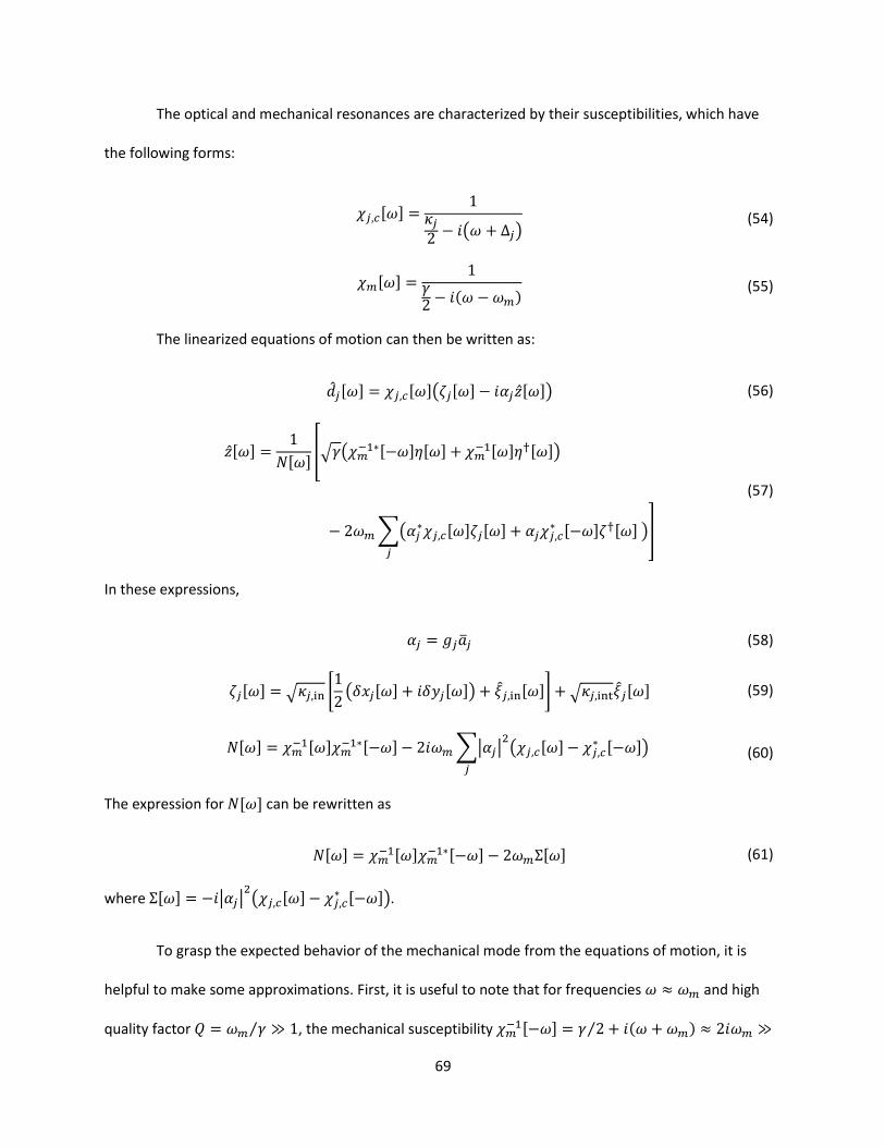
69

The optical and mechanical resonances are characterized by their susceptibilities, which have

the following forms:

𝜒𝑗,𝑐[𝜔] =1

𝜅𝑗2− 𝑖(𝜔 + Δ𝑗)

(54)

𝜒𝑚[𝜔] =1

𝛾2− 𝑖(𝜔 − 𝜔𝑚)

(55)

The linearized equations of motion can then be written as:

��𝑗[𝜔] = 𝜒𝑗,𝑐[𝜔](𝜁𝑗[𝜔] − 𝑖𝛼𝑗��[𝜔]) (56)

��[𝜔] =1

𝑁[𝜔][√𝛾(𝜒𝑚

−1∗[−𝜔]𝜂[𝜔] + 𝜒𝑚−1[𝜔]𝜂†[𝜔])

− 2𝜔𝑚∑(𝛼𝑗∗𝜒𝑗,𝑐[𝜔]𝜁𝑗[𝜔] + 𝛼𝑗𝜒𝑗,𝑐

∗ [−𝜔]𝜁†[𝜔] )

𝑗

]

(57)

In these expressions,

𝛼𝑗 = 𝑔𝑗��𝑗 (58)

𝜁𝑗[𝜔] = √𝜅𝑗,in [1

2(𝛿𝑥𝑗[𝜔] + 𝑖𝛿𝑦𝑗[𝜔]) + 𝜉𝑗,in[𝜔]] + √𝜅𝑗,int𝜉𝑗[𝜔] (59)

𝑁[𝜔] = 𝜒𝑚−1[𝜔]𝜒𝑚

−1∗[−𝜔] − 2𝑖𝜔𝑚∑|𝛼𝑗|2(𝜒𝑗,𝑐[𝜔] − 𝜒𝑗,𝑐

∗ [−𝜔])

𝑗

(60)

The expression for 𝑁[𝜔] can be rewritten as

𝑁[𝜔] = 𝜒𝑚−1[𝜔]𝜒𝑚

−1∗[−𝜔] − 2𝜔𝑚Σ[𝜔] (61)

where Σ[𝜔] = −𝑖|𝛼𝑗|2(𝜒𝑗,𝑐[𝜔] − 𝜒𝑗,𝑐

∗ [−𝜔]).

To grasp the expected behavior of the mechanical mode from the equations of motion, it is

helpful to make some approximations. First, it is useful to note that for frequencies 𝜔 ≈ 𝜔𝑚 and high

quality factor 𝑄 = 𝜔𝑚 𝛾⁄ ≫ 1, the mechanical susceptibility 𝜒𝑚−1[−𝜔] = 𝛾 2⁄ + 𝑖(𝜔 + 𝜔𝑚) ≈ 2𝑖𝜔𝑚 ≫

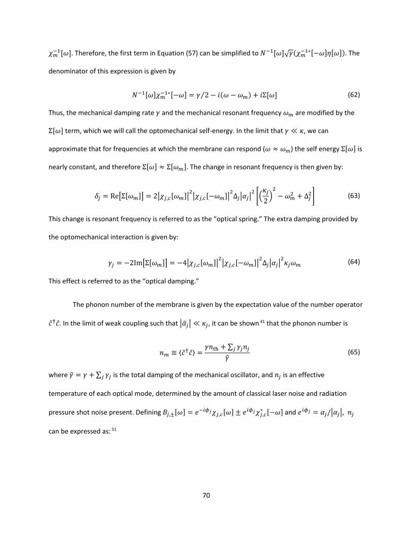
70

𝜒𝑚−1[𝜔]. Therefore, the first term in Equation (57) can be simplified to 𝑁−1[𝜔]√𝛾(𝜒𝑚

−1∗[−𝜔]𝜂[𝜔]). The

denominator of this expression is given by

𝑁−1[𝜔]𝜒𝑚−1∗[−𝜔] = 𝛾 2⁄ − 𝑖(𝜔 − 𝜔𝑚) + 𝑖Σ[𝜔] (62)

Thus, the mechanical damping rate 𝛾 and the mechanical resonant frequency 𝜔𝑚 are modified by the

Σ[𝜔] term, which we will call the optomechanical self-energy. In the limit that 𝛾 ≪ 𝜅, we can

approximate that for frequencies at which the membrane can respond (𝜔 ≈ 𝜔𝑚) the self energy Σ[𝜔] is

nearly constant, and therefore Σ[𝜔] ≈ Σ[𝜔𝑚]. The change in resonant frequency is then given by:

𝛿𝑗 = Re[Σ[𝜔𝑚]] = 2|𝜒𝑗,𝑐[𝜔𝑚]|2|𝜒𝑗,𝑐[−𝜔𝑚]|

2Δ𝑗|𝛼𝑗|

2[(𝜅𝑗

2)2

−𝜔𝑚2 + Δ𝑗

2] (63)

This change is resonant frequency is referred to as the “optical spring.” The extra damping provided by

the optomechanical interaction is given by:

𝛾𝑗 = −2Im[Σ[𝜔𝑚]] = −4|𝜒𝑗,𝑐[𝜔𝑚]|2|𝜒𝑗,𝑐[−𝜔𝑚]|

2Δ𝑗|𝛼𝑗|

2𝜅𝑗𝜔𝑚 (64)

This effect is referred to as the “optical damping.”

The phonon number of the membrane is given by the expectation value of the number operator

��†��. In the limit of weak coupling such that |��𝑗| ≪ 𝜅𝑗, it can be shown 41 that the phonon number is

𝑛𝑚 ≡ ⟨��†��⟩ =𝛾𝑛th +∑ 𝛾𝑗𝑛𝑗𝑗

�� (65)

where �� = 𝛾 + ∑ 𝛾𝑗𝑗 is the total damping of the mechanical oscillator, and 𝑛𝑗 is an effective

temperature of each optical mode, determined by the amount of classical laser noise and radiation

pressure shot noise present. Defining 𝐵𝑗,±[𝜔] = 𝑒−𝑖𝜙𝑗𝜒𝑗,𝑐[𝜔] ± 𝑒

𝑖𝜙𝑗𝜒𝑗,𝑐∗ [−𝜔] and 𝑒𝑖𝜙𝑗 = 𝛼𝑗/|𝛼𝑗|, 𝑛𝑗

can be expressed as: 51

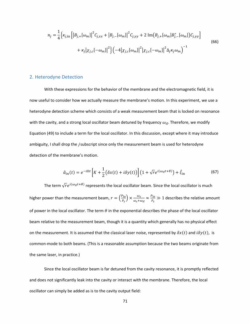
71

𝑛𝑗 =1

4{𝜅𝑗,in [|𝐵𝑗,+[𝜔𝑚]|

2𝐶𝑗,𝑥𝑥 + |𝐵𝑗,−[𝜔𝑚]|

2𝐶𝑗,𝑦𝑦 + 2 Im(𝐵𝑗,+[𝜔𝑚]𝐵𝑗,−

∗ [𝜔𝑚])𝐶𝑗,𝑦𝑦]

+ 𝜅𝑗|𝜒𝑗,𝑐[−𝜔𝑚]|2} (−4|𝜒𝑗,𝑐[𝜔𝑚]|

2|𝜒𝑗,𝑐[−𝜔𝑚]|

2Δ𝑗𝜅𝑗𝜔𝑚)

−1

(66)

2. Heterodyne Detection

With these expressions for the behavior of the membrane and the electromagnetic field, it is

now useful to consider how we actually measure the membrane’s motion. In this experiment, we use a

heterodyne detection scheme which consists of a weak measurement beam that is locked on resonance

with the cavity, and a strong local oscillator beam detuned by frequency 𝜔if. Therefore, we modify

Equation (49) to include a term for the local oscillator. In this discussion, except where it may introduce

ambiguity, I shall drop the j subscript since only the measurement beam is used for heterodyne

detection of the membrane’s motion.

��𝑖𝑛(𝑡) = 𝑒−𝑖Ω𝑡 [𝐾 +

1

2(𝛿𝑥(𝑡) + 𝑖𝛿𝑦(𝑡))] (1 + √𝑟𝑒𝑖(𝜔if𝑡+𝜃)) + 𝜉in (67)

The term √𝑟𝑒𝑖(𝜔if𝑡+𝜃) represents the local oscillator beam. Since the local oscillator is much

higher power than the measurement beam, 𝑟 = (𝑃lo

𝑃𝑠) ×

𝜔𝑠

𝜔𝑠+𝜔if≈

𝑃lo

𝑃𝑠≫ 1 describes the relative amount

of power in the local oscillator. The term 𝜃 in the exponential describes the phase of the local oscillator

beam relative to the measurement beam, though it is a quantity which generally has no physical effect

on the measurement. It is assumed that the classical laser noise, represented by 𝛿𝑥(𝑡) and 𝑖𝛿𝑦(𝑡), is

common-mode to both beams. (This is a reasonable assumption because the two beams originate from

the same laser, in practice.)

Since the local oscillator beam is far detuned from the cavity resonance, it is promptly reflected

and does not significantly leak into the cavity or interact with the membrane. Therefore, the local

oscillator can simply be added as is to the cavity output field:

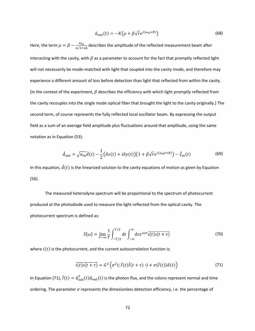
72

��out(𝑡) = −𝐾(𝜌 + 𝛽√𝑟𝑒𝑖(𝜔if+𝜃)) (68)

Here, the term 𝜌 = 𝛽 −𝜅in

𝜅 2⁄ +𝑖Δ describes the amplitude of the reflected measurement beam after

interacting with the cavity, with 𝛽 as a parameter to account for the fact that promptly reflected light

will not necessarily be mode-matched with light that coupled into the cavity mode, and therefore may

experience a different amount of loss before detection than light that reflected from within the cavity.

(In the context of the experiment, 𝛽 describes the efficiency with which light promptly reflected from

the cavity recouples into the single mode optical fiber that brought the light to the cavity originally.) The

second term, of course represents the fully reflected local oscillator beam. By expressing the output

field as a sum of an average field amplitude plus fluctuations around that amplitude, using the same

notation as in Equation (53):

��out = √𝜅in��(𝑡) −1

2(𝛿𝑥(𝑡) + 𝑖𝛿𝑦(𝑡))(1 + 𝛽√𝑟𝑒𝑖(𝜔if𝑡+𝜃)) − 𝜉in(𝑡) (69)

In this equation, ��(𝑡) is the linearized solution to the cavity equations of motion as given by Equation

(56).

The measured heterodyne spectrum will be proportional to the spectrum of photocurrent

produced at the photodiode used to measure the light reflected from the optical cavity. The

photocurrent spectrum is defined as:

𝑆[𝜔] = lim𝑇→∞

1

𝑇∫ d𝑡𝑇/2

−𝑇/2

∫ d𝜏𝑒𝑖𝜔𝜏𝑖(𝑡)𝑖(𝑡 + 𝜏) ∞

−∞

(70)

where 𝑖(𝑡) is the photocurrent, and the current autocorrelation function is:

𝑖(𝑡)𝑖(𝑡 + 𝜏) = 𝐺2 (𝜎2⟨: 𝐼(𝑡)𝐼(𝑡 + 𝜏) ∶⟩ + 𝜎⟨𝐼(𝑡)⟩𝛿(𝑡)) (71)

In Equation (71), 𝐼(𝑡) = ��out† (𝑡)��out(𝑡) is the photon flux, and the colons represent normal and time

ordering. The parameter 𝜎 represents the dimesionless detection efficiency, i.e. the percentage of

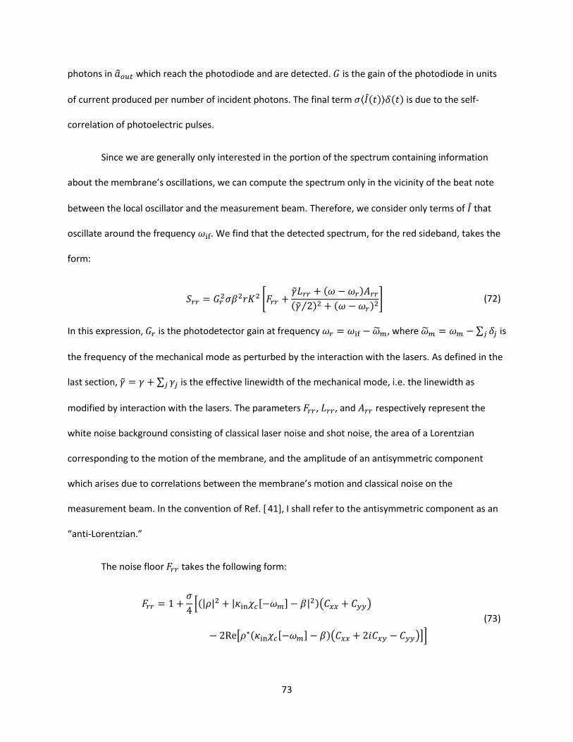
73

photons in ��𝑜𝑢𝑡 which reach the photodiode and are detected. 𝐺 is the gain of the photodiode in units

of current produced per number of incident photons. The final term 𝜎⟨𝐼(𝑡)⟩𝛿(𝑡) is due to the self-

correlation of photoelectric pulses.

Since we are generally only interested in the portion of the spectrum containing information

about the membrane’s oscillations, we can compute the spectrum only in the vicinity of the beat note

between the local oscillator and the measurement beam. Therefore, we consider only terms of 𝐼 that

oscillate around the frequency 𝜔if. We find that the detected spectrum, for the red sideband, takes the

form:

𝑆𝑟𝑟 = 𝐺𝑟2𝜎𝛽2𝑟𝐾2 [𝐹𝑟𝑟 +

��𝐿𝑟𝑟 + (𝜔 − 𝜔𝑟)𝐴𝑟𝑟(�� 2⁄ )2 + (𝜔 − 𝜔𝑟)

2] (72)

In this expression, 𝐺𝑟 is the photodetector gain at frequency 𝜔𝑟 = 𝜔if − ��𝑚, where ��𝑚 = 𝜔𝑚 −∑ 𝛿𝑗𝑗 is

the frequency of the mechanical mode as perturbed by the interaction with the lasers. As defined in the

last section, �� = 𝛾 + ∑ 𝛾𝑗𝑗 is the effective linewidth of the mechanical mode, i.e. the linewidth as

modified by interaction with the lasers. The parameters 𝐹𝑟𝑟, 𝐿𝑟𝑟, and 𝐴𝑟𝑟 respectively represent the

white noise background consisting of classical laser noise and shot noise, the area of a Lorentzian

corresponding to the motion of the membrane, and the amplitude of an antisymmetric component

which arises due to correlations between the membrane’s motion and classical noise on the

measurement beam. In the convention of Ref. [ 41], I shall refer to the antisymmetric component as an

“anti-Lorentzian.”

The noise floor 𝐹𝑟𝑟 takes the following form:

𝐹𝑟𝑟 = 1 +𝜎

4[(|𝜌|2 + |𝜅in𝜒𝑐[−𝜔𝑚] − 𝛽|

2)(𝐶𝑥𝑥 + 𝐶𝑦𝑦)

− 2Re[𝜌∗(𝜅in𝜒𝑐[−𝜔𝑚] − 𝛽)(𝐶𝑥𝑥 + 2𝑖𝐶𝑥𝑦 − 𝐶𝑦𝑦)]]

(73)

74

In this expression, all noises have been normalized to shot noise – therefore the 1 at the beginning of

the expression is shot noise itself. The other terms represent contributions from classical laser noise,

and scale linearly in power.

The Lorentzian component of Equation (72) is

𝐿𝑟𝑟 = 𝜎𝜅in|𝛼|2|𝜒𝑐[−𝜔𝑚]|

2(𝑛𝑚 + 1) + Re��[𝜔𝑚] (74)

�� represents the effects of classical noise on 𝐿𝑟𝑟 (and 𝐴𝑟𝑟). Using the definition of 𝐵±[𝜔] from the last

section, �� takes the form:

��[𝜔] =𝜅in4|𝜒𝑐[−𝜔]|

2𝑒−𝑖𝜙 [(𝐶𝑥𝑥 + 𝑖𝐶𝑥𝑦)𝐵+[𝜔] + (𝑖𝐶𝑥𝑦 − 𝐶𝑦𝑦)𝐵−[𝜔]]

−𝛽

4𝜒𝑐∗[−𝜔]𝑒−𝑖𝜙[(𝐶𝑥𝑥𝐵+[𝜔] + 𝑖𝐶𝑥𝑦𝐵−[𝜔])(1 + 𝜌)

+ (𝑖𝐶𝑥𝑦𝐵+[𝜔] − 𝐶𝑦𝑦𝐵−[𝜔])(1 − 𝜌)]

(75)

The anti-Lorentzian component of Equation (72) is:

𝐴𝑟𝑟 = 2𝜎𝜅in|𝛼|2 Im ��[𝜔𝑚] (76)

The heterodyne spectrum of the blue sideband has a form very similar to that of the red

sideband, except for a few subtle differences: namely, the sign of 𝜔𝑚 is switched since this sideband

occurs at a frequency higher than 𝜔if, �� is subtracted instead of added, and (𝑛𝑚 + 1) → 𝑛𝑚 in the

expression for 𝐿𝑏𝑏. Explicitly, these expressions are:

𝑆𝑏𝑏 = 𝐺𝑏2𝜎𝛽2𝑟𝐾2 [𝐹𝑟𝑟 +

��𝐿𝑟𝑟 + (𝜔 − 𝜔𝑏)𝐴𝑟𝑟(�� 2⁄ )2 + (𝜔 − 𝜔𝑏)

2] (77)

In Equation (77), analogous to 𝜔𝑟, 𝜔𝑏 = 𝜔if + ��𝑚.

𝐹𝑏𝑏 = 1 +𝜎

4[(|𝜌|2 + |𝜅in𝜒𝑐[𝜔𝑚] − 𝛽|

2)(𝐶𝑥𝑥 + 𝐶𝑦𝑦)

− 2Re[𝜌∗(𝜅in𝜒𝑐[𝜔𝑚] − 𝛽)(𝐶𝑥𝑥 + 2𝑖𝐶𝑥𝑦 − 𝐶𝑦𝑦)]]

(78)

75

𝐿𝑏𝑏 = 𝜎𝜅in|𝛼|2|𝜒𝑐[𝜔𝑚]|

2(𝑛𝑚) − Re��[−𝜔𝑚] (79)

𝐴𝑏𝑏 = −2𝜎𝜅in|𝛼|2 Im ��[−𝜔𝑚] (80)

So far in this discussion I have neglected the cooling beam since it does not contribute any

information about the membrane’s motion to the photocurrent spectrum around 𝜔if. However, it does

still make a white contribution to the spectrum from shot noise. This contribution takes the form

𝑆𝑟𝑟,𝑝 = 𝐺𝑟

2𝜎𝛽2𝐾𝑝2|𝜌𝑝|

2

𝑆𝑏𝑏,𝑝 = 𝐺𝑏2𝜎𝛽2𝐾𝑝

2|𝜌𝑝|2

(81)

for the red and the blue sidebands respectively. These expressions may be added to Equations (72) and

(77) to produce the full expressions for the heterodyne spectrum in cases where absolute calibration the

white background is important.

The origin and interpretation of the asymmetry in the dependence on 𝑛𝑚 in the expressions for

𝐿𝑟𝑟 and 𝐿𝑏𝑏 are non-trivial, and are treated in Ref.[ 8]. Summarized briefly, for a linear power detector

like the photodiode used in this experiment, there are four physical contributions to 𝑆𝑟𝑟 and 𝑆𝑏𝑏:

1. Quantum fluctuations of the electromagnetic field, which manifest as shot noise.

2. Thermal motion of the mechanical oscillator, which produces sidebands of equal area, each

proportional to the mean phonon number of the mechanical oscillator 𝑛𝑚 ≈ 𝑘B𝑇/ℏ𝜔𝑚.

3. Zero-point motion of the oscillator, which contributes equally to each of the sidebands by an

amount equivalent to increasing the oscillator’s mean phonon number by ½.

4. The response of the oscillator to the quantum fluctuations of the electromagnetic field,

which contributes to the red sideband by an amount equivalent to increasing the mean

phonon number by ½, and to the blue sideband by an amount equivalent to decreasing the

mean phonon number by ½.

76

Contributions 2-4 together indicate that 𝐿𝑟𝑟 should have an area that is equal to the area that

would be expected if the oscillator had one more phonon than it really does, while 𝐿𝑏𝑏 should scale

linearly with phonon number all the way down to zero. These contributions are summarized

schematically in Figure 14.

Figure 14: Schematic representation of contributions to the red (left) and blue (right) sidebands for a membrane with phonon number 𝑛𝑚 = 0. The dashed green line represents the contribution due to the quantum fluctuations of the electromagnetic field

(shot noise), the red dashed line represents the contribution due to the oscillator’s zero-point motion, and the blue represents the contribution due to the response of the oscillator to the quantum fluctuations of the electromagnetic field. Since this

diagram is for 𝑛𝑚 = 0, there is no contribution from the oscillator’s thermal motion.

Using this description of the asymmetry of the sidebands, it is possible to compute the mean

phonon number by comparing the ratio of the sideband areas. This can be done by subtracting the 𝐹𝑟𝑟

and 𝐹𝑏𝑏 background terms from Equations (72) and (77), normalizing the gain of one sideband to the

gain of the other, then integrate the remaining terms over all frequency space. The result of this integral

is referred to as the “sideband weight”, which is essentially just 𝐿𝑟𝑟 and 𝐿𝑏𝑏 normalized so that they may

be directly compared. 51 Taking the ratio of the red sideband weight to the blue sideband weight gives

the sideband ratio, which we define as 𝜉:

𝜉 =𝑊𝑟𝑟𝑊𝑏𝑏

=|𝜒𝑐[−𝜔𝑚]|

2(𝑛𝑚 + 1) + Re ��[𝜔𝑚]

|𝜒𝑐[𝜔𝑚]|2𝑛𝑚 − Re ��[−𝜔𝑚]

(82)

In the absence of classical laser noise, �� ≡ 0. If the measurement laser is exactly on resonance

with the optical cavity (measurement beam detuning Δ𝑠 = 0), then |𝜒𝑐[𝜔]|2 is an even function and the

sideband ratio 𝜉 depends only on the mean phonon number:

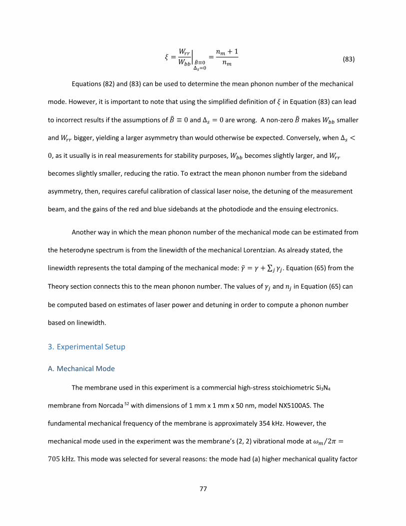
77

𝜉 =𝑊𝑟𝑟𝑊𝑏𝑏

|��≡0Δ𝑠=0

=𝑛𝑚 + 1

𝑛𝑚 (83)

Equations (82) and (83) can be used to determine the mean phonon number of the mechanical

mode. However, it is important to note that using the simplified definition of 𝜉 in Equation (83) can lead

to incorrect results if the assumptions of �� ≡ 0 and Δ𝑠 = 0 are wrong. A non-zero �� makes 𝑊𝑏𝑏 smaller

and 𝑊𝑟𝑟 bigger, yielding a larger asymmetry than would otherwise be expected. Conversely, when Δ𝑠 <

0, as it usually is in real measurements for stability purposes, 𝑊𝑏𝑏 becomes slightly larger, and 𝑊𝑟𝑟

becomes slightly smaller, reducing the ratio. To extract the mean phonon number from the sideband

asymmetry, then, requires careful calibration of classical laser noise, the detuning of the measurement

beam, and the gains of the red and blue sidebands at the photodiode and the ensuing electronics.

Another way in which the mean phonon number of the mechanical mode can be estimated from

the heterodyne spectrum is from the linewidth of the mechanical Lorentzian. As already stated, the

linewidth represents the total damping of the mechanical mode: �� = 𝛾 + ∑ 𝛾𝑗𝑗 . Equation (65) from the

Theory section connects this to the mean phonon number. The values of 𝛾𝑗 and 𝑛𝑗 in Equation (65) can

be computed based on estimates of laser power and detuning in order to compute a phonon number

based on linewidth.

3. Experimental Setup

A. Mechanical Mode

The membrane used in this experiment is a commercial high-stress stoichiometric Si3N4

membrane from Norcada 52 with dimensions of 1 mm x 1 mm x 50 nm, model NX5100AS. The

fundamental mechanical frequency of the membrane is approximately 354 kHz. However, the

mechanical mode used in the experiment was the membrane’s (2, 2) vibrational mode at 𝜔𝑚 2𝜋⁄ =

705 kHz. This mode was selected for several reasons: the mode had (a) higher mechanical quality factor

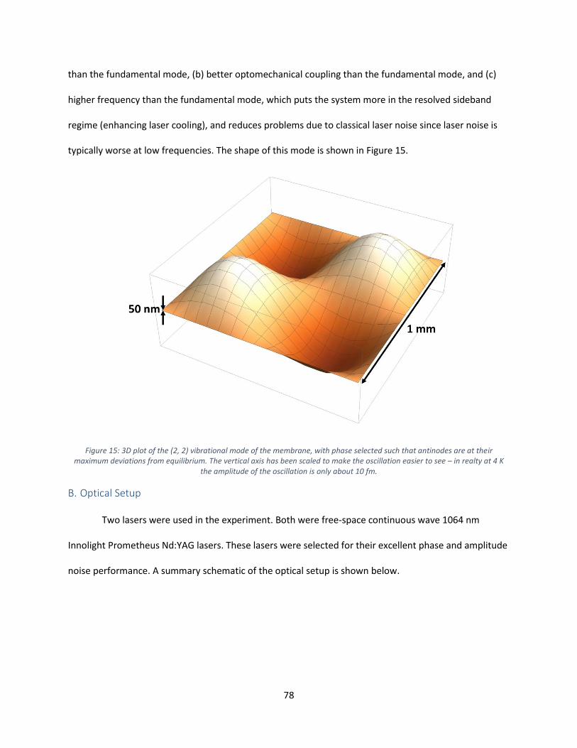
78

than the fundamental mode, (b) better optomechanical coupling than the fundamental mode, and (c)

higher frequency than the fundamental mode, which puts the system more in the resolved sideband

regime (enhancing laser cooling), and reduces problems due to classical laser noise since laser noise is

typically worse at low frequencies. The shape of this mode is shown in Figure 15.

Figure 15: 3D plot of the (2, 2) vibrational mode of the membrane, with phase selected such that antinodes are at their maximum deviations from equilibrium. The vertical axis has been scaled to make the oscillation easier to see – in realty at 4 K

the amplitude of the oscillation is only about 10 fm.

B. Optical Setup

Two lasers were used in the experiment. Both were free-space continuous wave 1064 nm

Innolight Prometheus Nd:YAG lasers. These lasers were selected for their excellent phase and amplitude

noise performance. A summary schematic of the optical setup is shown below.

79

Figure 16: Schematic of the optical setup for the ground state cooling experiment.

The measurement laser, labelled “ML” in Figure 16, first passes through a beamsplitter which

picks off a small percentage of the beam to use as a reference for measuring the frequency difference

between the measurement laser and the cooling laser (labelled “CL” in Figure 16). The rest of the

measurement laser passes through an optical filter cavity labelled “FC1”. (I will explain more about how

the filter cavity works in the next section.) The filter cavity is locked to the measurement laser using a

Pound-Drever-Hall locking technique, 38 with feedback going to a piezo actuator that changes the length

of the optical cavity to keep it on resonance with the laser. Light that transmits through the filter cavity

goes through a beamsplitter which breaks it into two paths. One path goes through an electrooptic

modulator (EOM) which produces phase modulation sidebands for Pound-Drever-Hall locking to the

cryogenic optical cavity. It also passes through an acoustooptic modulator (AOM1), which shifts its

frequency by 80 MHz so that it can be used for heterodyne detection. This beam is referred to as the

“measurement beam” or the “probe beam”. The other path from the beamsplitter doesn’t pass through

any modulators, and is used as and referred to as the “local oscillator” beam. The two beams are

recombined in another beam splitter, before being coupled into an optical fiber.

80

Once in the optical fiber, the measurement laser passes through a wide bandwidth fiber

acoustooptic modulator (AOM2). The servo used to keep the measurement beam locked to the

cryogenic optical cavity works by changing the drive frequency of AOM2. After passing through AOM2,

the measurement beam goes through a fiber optic circulator which sends the beam into the cryostat.

Once in the cryostat, the measurement beam enters the optical cavity and interacts with the

membrane, acquiring phase modulation sidebands containing information about the membrane’s

motion at ±𝜔𝑚. The local oscillator beam goes into the cryostat, but is 80 MHz away from the cavity

resonance, and promptly reflects from the input mirror. Both beams recouple into the same optical fiber

that took them into the cryostat originally, and are diverted by the fiber optic circulator to a Thorlabs

PDA10CF photodiode for measurement. In Figure 16, the measurement apparatus is labelled “DAQ”.

The cooling laser, like the measurement laser, has a small percentage picked off to combine

with the light that was picked off from the measurement laser. The two beams combine using a

beamsplitter and land on a fast photodiode which can detect the several GHz beat note between the

two lasers. The signal from this photodiode goes through a mixing circuit and then to a servo which

feeds back to the laser piezo in the cooling laser to lock it a fixed frequency difference away from the

measurement laser (more information about this in the Laser Locking Setup section). The rest of the

cooling laser passes through another filter cavity, labelled “FC2”, which is locked to the cooling laser

using a similar technique to FC1. After passing through the filter cavity, the cooling laser goes through

some waveplates and a polarizer (not shown in Figure 16), which are used to adjust the optical power of

the cooling beam. The cooling beam then couples into an optical fiber and is combined with the

measurement laser using a polarizing beam combiner, following the same path into the cryostat and

back. Since the cooling beam passes through AOM2 just like the measurement beam, it acquires the

same frequency shifts as the measurement beam, allowing it to track the fluctuations of the cold cavity.

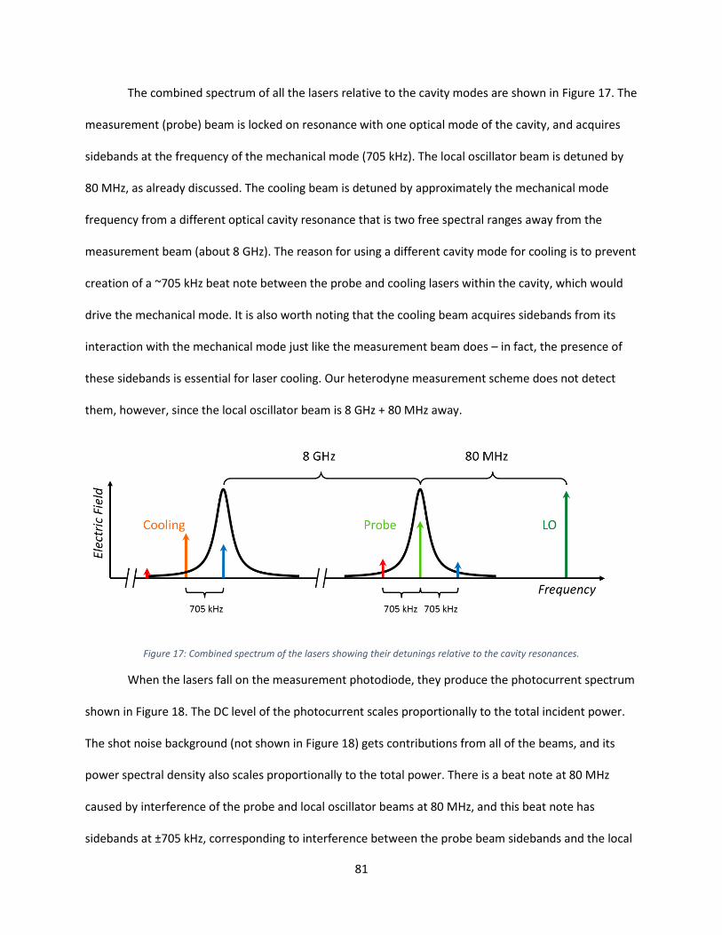
81

The combined spectrum of all the lasers relative to the cavity modes are shown in Figure 17. The

measurement (probe) beam is locked on resonance with one optical mode of the cavity, and acquires

sidebands at the frequency of the mechanical mode (705 kHz). The local oscillator beam is detuned by

80 MHz, as already discussed. The cooling beam is detuned by approximately the mechanical mode

frequency from a different optical cavity resonance that is two free spectral ranges away from the

measurement beam (about 8 GHz). The reason for using a different cavity mode for cooling is to prevent

creation of a ~705 kHz beat note between the probe and cooling lasers within the cavity, which would

drive the mechanical mode. It is also worth noting that the cooling beam acquires sidebands from its

interaction with the mechanical mode just like the measurement beam does – in fact, the presence of

these sidebands is essential for laser cooling. Our heterodyne measurement scheme does not detect

them, however, since the local oscillator beam is 8 GHz + 80 MHz away.

Figure 17: Combined spectrum of the lasers showing their detunings relative to the cavity resonances.

When the lasers fall on the measurement photodiode, they produce the photocurrent spectrum

shown in Figure 18. The DC level of the photocurrent scales proportionally to the total incident power.

The shot noise background (not shown in Figure 18) gets contributions from all of the beams, and its

power spectral density also scales proportionally to the total power. There is a beat note at 80 MHz

caused by interference of the probe and local oscillator beams at 80 MHz, and this beat note has

sidebands at ±705 kHz, corresponding to interference between the probe beam sidebands and the local

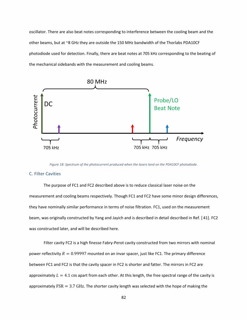
82

oscillator. There are also beat notes corresponding to interference between the cooling beam and the

other beams, but at ~8 GHz they are outside the 150 MHz bandwidth of the Thorlabs PDA10CF

photodiode used for detection. Finally, there are beat notes at 705 kHz corresponding to the beating of

the mechanical sidebands with the measurement and cooling beams.

Figure 18: Spectrum of the photocurrent produced when the lasers land on the PDA10CF photodiode.

C. Filter Cavities

The purpose of FC1 and FC2 described above is to reduce classical laser noise on the

measurement and cooling beams respectively. Though FC1 and FC2 have some minor design differences,

they have nominally similar performance in terms of noise filtration. FC1, used on the measurement

beam, was originally constructed by Yang and Jayich and is described in detail described in Ref. [ 41]. FC2

was constructed later, and will be described here.

Filter cavity FC2 is a high finesse Fabry-Perot cavity constructed from two mirrors with nominal

power reflectivity 𝑅 = 0.99997 mounted on an invar spacer, just like FC1. The primary difference

between FC1 and FC2 is that the cavity spacer in FC2 is shorter and fatter. The mirrors in FC2 are

approximately 𝐿 = 4.1 cm apart from each other. At this length, the free spectral range of the cavity is

approximately FSR = 3.7 GHz. The shorter cavity length was selected with the hope of making the

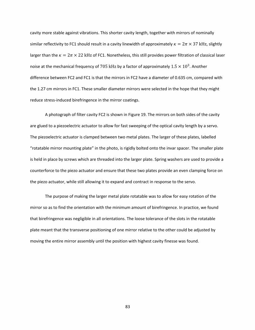
83

cavity more stable against vibrations. This shorter cavity length, together with mirrors of nominally

similar reflectivity to FC1 should result in a cavity linewidth of approximately 𝜅 = 2𝜋 × 37 kHz, slightly

larger than the 𝜅 = 2𝜋 × 22 kHz of FC1. Nonetheless, this still provides power filtration of classical laser

noise at the mechanical frequency of 705 kHz by a factor of approximately 1.5 × 103. Another

difference between FC2 and FC1 is that the mirrors in FC2 have a diameter of 0.635 cm, compared with

the 1.27 cm mirrors in FC1. These smaller diameter mirrors were selected in the hope that they might

reduce stress-induced birefringence in the mirror coatings.

A photograph of filter cavity FC2 is shown in Figure 19. The mirrors on both sides of the cavity

are glued to a piezoelectric actuator to allow for fast sweeping of the optical cavity length by a servo.

The piezoelectric actuator is clamped between two metal plates. The larger of these plates, labelled

“rotatable mirror mounting plate” in the photo, is rigidly bolted onto the invar spacer. The smaller plate

is held in place by screws which are threaded into the larger plate. Spring washers are used to provide a

counterforce to the piezo actuator and ensure that these two plates provide an even clamping force on

the piezo actuator, while still allowing it to expand and contract in response to the servo.

The purpose of making the larger metal plate rotatable was to allow for easy rotation of the

mirror so as to find the orientation with the minimum amount of birefringence. In practice, we found

that birefringence was negligible in all orientations. The loose tolerance of the slots in the rotatable

plate meant that the transverse positioning of one mirror relative to the other could be adjusted by

moving the entire mirror assembly until the position with highest cavity finesse was found.

84

Figure 19: Photograph of filter cavity FC2.

A kinematic mount inside a vacuum can provides a reliable mount for the filter cavity within the

optical beam path. Sapphire balls sit between the cavity spacer and the mount. One large ball mates

with the cone which can be seen in photograph above, and the other balls touch the outer cylindrical

surface of the invar spacer. The combination of all these contact points ensures repeatable positioning

of the cavity within the optical beam path so that the cavity can be removed, adjusted, and reseated

without requiring extensive optical realignment. The CAD drawing in Figure 20 shows how the filter

cavity sits on this mount.

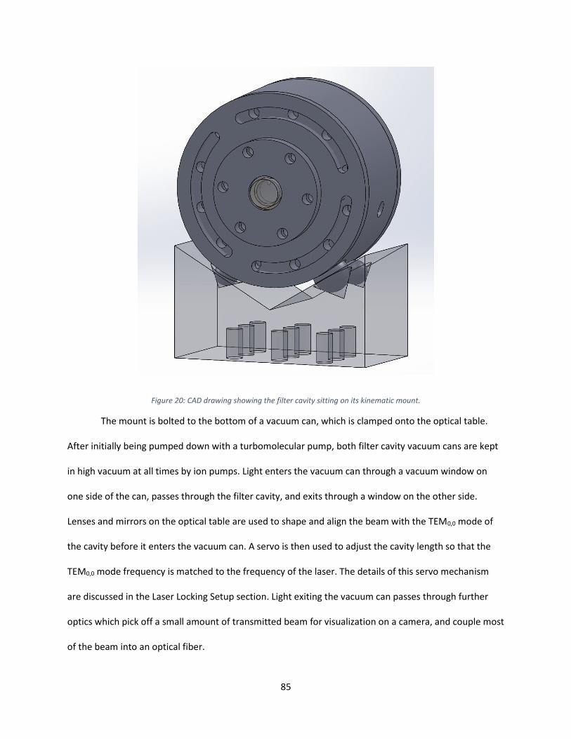
85

Figure 20: CAD drawing showing the filter cavity sitting on its kinematic mount.

The mount is bolted to the bottom of a vacuum can, which is clamped onto the optical table.

After initially being pumped down with a turbomolecular pump, both filter cavity vacuum cans are kept

in high vacuum at all times by ion pumps. Light enters the vacuum can through a vacuum window on

one side of the can, passes through the filter cavity, and exits through a window on the other side.

Lenses and mirrors on the optical table are used to shape and align the beam with the TEM0,0 mode of

the cavity before it enters the vacuum can. A servo is then used to adjust the cavity length so that the

TEM0,0 mode frequency is matched to the frequency of the laser. The details of this servo mechanism

are discussed in the Laser Locking Setup section. Light exiting the vacuum can passes through further

optics which pick off a small amount of transmitted beam for visualization on a camera, and couple most

of the beam into an optical fiber.

86

With perfect mode matching to a lossless, symmetrical optical cavity, it should be possible to

obtain 100% transmission of a shot noise limited laser that is on resonance with the cavity. In practice,

primarily due to imperfect mode matching, we typically obtain at best 50% transmission. In spite of this

power loss, the light exiting the cavity has significantly less classical laser noise than the light incident on

the cavity due to filtration by the cavity. Filtration of classical laser noise occurs passively due to the

narrow linewidth of the cavity. The noise power filtration factor is given by the ratio of the squared

cavity susceptibility measured on resonance to the squared cavity susceptibility at the frequency of the

noise, i.e. |𝜒FC[0]|2/|𝜒FC[Δnoise]|

2, where 𝜒FC[𝜔] is the cavity susceptibility and Δnoise is the detuning

of the noise relative to the cavity resonance.

While this reduction in noise is desirable during attempts to cool the membrane to the ground

state, the extra steps involved to lock the filter cavities can be burdensome for miscellaneous

measurements and general experimental tasks that don’t require shot noise limited performance.

Therefore the optics surrounding the filter cavities have been laid out such that either filter cavity may

be bypassed on demand via removable mirrors in the beam path. Engaging the bypass of either FC1 or

FC2 has the net effect of completely removing the filter cavity, its preceding beamsplitter, and its servo

loop from the summary schematic in Figure 16.

A photograph of the complete FC2 optical setup is shown in Figure 21 below.

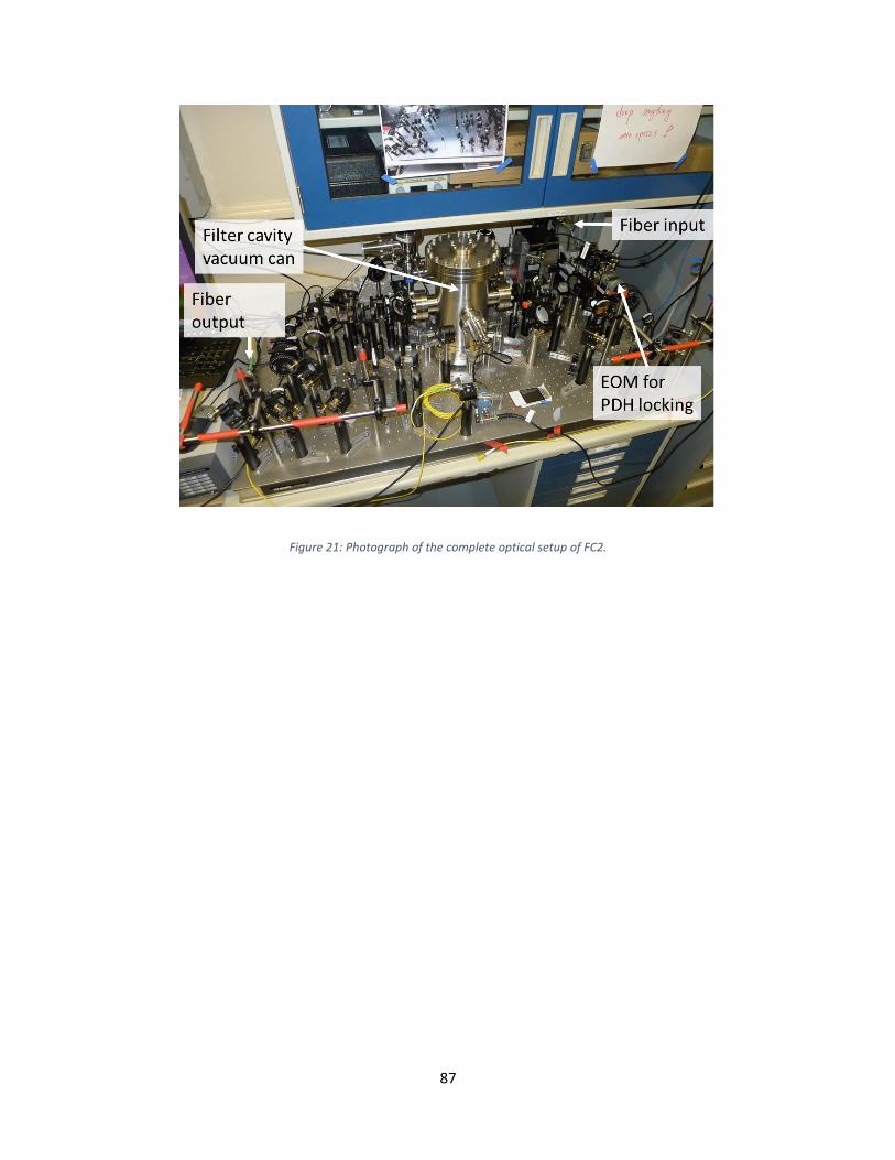
87

Figure 21: Photograph of the complete optical setup of FC2.

88

D. Cryogenic Setup

The cryogenics system used in this experiment is a Janis 3He refrigerator. It consists of an

internal vacuum chamber (IVC) which is submerged in a bath of liquid 4He at a temperature of ~4 K. This

bath has to be replenished approximately once per week by transferring liquid helium from a storage

dewar provided by a supplier. Within the IVC is a series of cryogenic stages that achieve temperatures as

low as 300 mK by evaporative cooling of liquid 3He in a sealed chamber. A charcoal “sorb” adsorbs

evaporated 3He atoms to prevent 3He vapor pressure from rising over the liquid and slowing the

evaporative cooling process. Eventually, all the 3He in the system evaporates and is adsorbed in sorb, at

which point the temperature of the system rises to the bath temperature of 4 K. To cool the system

down again, it is necessary to run a refrigeration cycle which consists of heating the sorb to release the

adsorbed 3He, and pumping on a small chamber of 4He with a mechanical pump to achieve

temperatures low enough to condense the 3He back into a liquid. Once most of the 3He has been

recondensed, the sorb heater and mechanical pump are switched off, allowing for evaporative cooling

of the liquid 3He to resume. This recondensation cycle needs to be performed approximately once per

week.

The use of a sorb-pumped 3He refrigerator is nice because during normal operation, there are

no mechanical pumps running, keeping vibrations to a minimum. However, the tradeoff for this

normally quiet operation is an unavoidable weekly warm up of the experimental apparatus in the IVC to

4 K during the recondensation process. While the experimental apparatus about to be discussed

generally tolerates this brief thermal excursion quite well, it sometimes can have effects on the system,

as will be discussed.

The cryogenic “stage” of the membrane-in-the-middle experiment is stored entirely within the

IVC, and is coupled to the coldest part of the 3He refrigerator. Due to thermal conductivity through

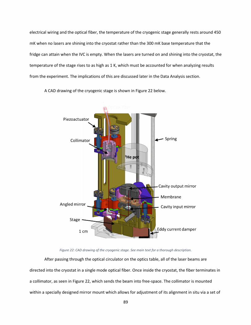
89

electrical wiring and the optical fiber, the temperature of the cryogenic stage generally rests around 450

mK when no lasers are shining into the cryostat rather than the 300 mK base temperature that the

fridge can attain when the IVC is empty. When the lasers are turned on and shining into the cryostat, the

temperature of the stage rises to as high as 1 K, which must be accounted for when analyzing results

from the experiment. The implications of this are discussed later in the Data Analysis section.

A CAD drawing of the cryogenic stage is shown in Figure 22 below.

Figure 22: CAD drawing of the cryogenic stage. See main text for a thorough description.

After passing through the optical circulator on the optics table, all of the laser beams are

directed into the cryostat in a single mode optical fiber. Once inside the cryostat, the fiber terminates in

a collimator, as seen in Figure 22, which sends the beam into free-space. The collimator is mounted

within a specially designed mirror mount which allows for adjustment of its alignment in situ via a set of

90

three piezo-actuated mirror knobs. The knobs, appropriately called PiezoKnobs, are computer-

controlled actuators that can adjust all the degrees of freedom of the mirror mount even at cryogenic

temperatures.

The free-space beam coming out of the collimator travels downward and hits an adjustable 45

degree mirror, which is mounted in a similar piezo-actuated mirror mount. Since both the collimator and

this mirror can be adjusted on multiple axes, it is possible to use two-knob-adjustment techniques to

align the beams with the cryogenic cavity for optimal mode matching.

The light from the adjustable 45 degree mirror bounces off another non-adjustable 45 degree

mirror which directs it toward the cavity input mirror. If well coupled and tuned to the right frequency,

light enters the cavity and interacts with the membrane. The membrane itself is mounted on a

somewhat larger, but otherwise similar piezo-actuated mirror mount. This allows for adjustment of the

membrane’s tip, tilt, and translation along the cavity axis.

The cavity output mirror (𝑅 = 0.99997) was selected to be significantly more reflective than the

input mirror (𝑅 = 0.9998), so that most of the light within the cavity reflects and traces the same path

back to collimator and optical fiber. Light that manages to recouple into the fiber returns to the optical

table for measurement.

Light that transmits through the cavity’s output mirror is collected on a germanium photodiode

(not shown in Figure 22). The photodiode is not particularly useful for measurement of the mechanical

mode due to the poor responsivity of germanium photodiodes at 1064 nm at cryogenic temperatures,

and also the high RC time constant of that photodiode and its readout electronics system. Nonetheless,

the transmission photodiode is useful for initial alignment of the system at cryogenic temperatures

using 935 nm light, as will be discussed in the next section.

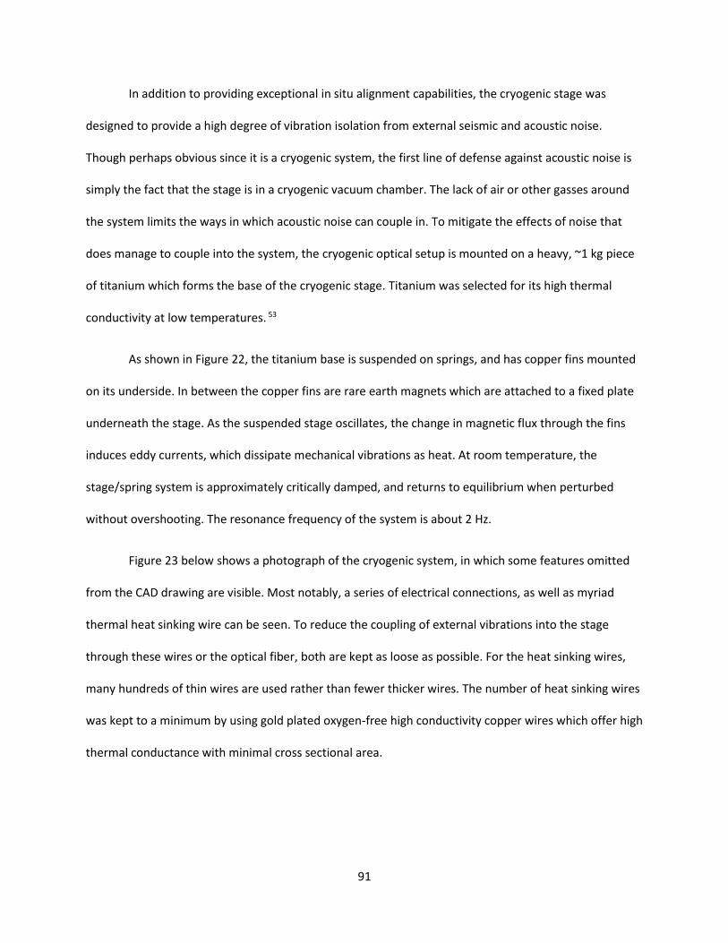
91

In addition to providing exceptional in situ alignment capabilities, the cryogenic stage was

designed to provide a high degree of vibration isolation from external seismic and acoustic noise.

Though perhaps obvious since it is a cryogenic system, the first line of defense against acoustic noise is

simply the fact that the stage is in a cryogenic vacuum chamber. The lack of air or other gasses around

the system limits the ways in which acoustic noise can couple in. To mitigate the effects of noise that

does manage to couple into the system, the cryogenic optical setup is mounted on a heavy, ~1 kg piece

of titanium which forms the base of the cryogenic stage. Titanium was selected for its high thermal

conductivity at low temperatures. 53

As shown in Figure 22, the titanium base is suspended on springs, and has copper fins mounted

on its underside. In between the copper fins are rare earth magnets which are attached to a fixed plate

underneath the stage. As the suspended stage oscillates, the change in magnetic flux through the fins

induces eddy currents, which dissipate mechanical vibrations as heat. At room temperature, the

stage/spring system is approximately critically damped, and returns to equilibrium when perturbed

without overshooting. The resonance frequency of the system is about 2 Hz.

Figure 23 below shows a photograph of the cryogenic system, in which some features omitted

from the CAD drawing are visible. Most notably, a series of electrical connections, as well as myriad

thermal heat sinking wire can be seen. To reduce the coupling of external vibrations into the stage

through these wires or the optical fiber, both are kept as loose as possible. For the heat sinking wires,

many hundreds of thin wires are used rather than fewer thicker wires. The number of heat sinking wires

was kept to a minimum by using gold plated oxygen-free high conductivity copper wires which offer high

thermal conductance with minimal cross sectional area.

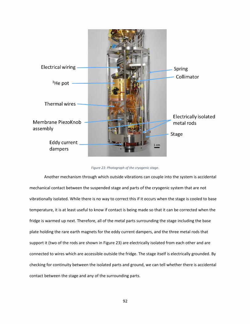
92

Figure 23: Photograph of the cryogenic stage.

Another mechanism through which outside vibrations can couple into the system is accidental

mechanical contact between the suspended stage and parts of the cryogenic system that are not

vibrationally isolated. While there is no way to correct this if it occurs when the stage is cooled to base

temperature, it is at least useful to know if contact is being made so that it can be corrected when the

fridge is warmed up next. Therefore, all of the metal parts surrounding the stage including the base

plate holding the rare earth magnets for the eddy current dampers, and the three metal rods that

support it (two of the rods are shown in Figure 23) are electrically isolated from each other and are

connected to wires which are accessible outside the fridge. The stage itself is electrically grounded. By

checking for continuity between the isolated parts and ground, we can tell whether there is accidental

contact between the stage and any of the surrounding parts.

93

For further isolation, the cryostat itself sits on four pneumatic vibration isolators. These

isolators, Newport Model S-2000A-128, are typically used to support and isolate optical tables. As can be

seen in Figure 24, a heavy duty aluminum frame made of 8020 brand extrusions rests on top of the of

vibration isolators. The frame supports a thick aluminum plate in the middle to which the dewar is

bolted and suspended (not shown in Figure 24). Surrounding the dewar setup are removable walls and a

ceiling made of plexi-glass that are covered in soundproofing foam to reduce the influence of acoustic

noise. When fully enclosed within this acoustic isolation cube, the ambient sound levels around the

dewar are reduced by 13 dB.

Figure 24: A top down photograph of the cryostat during assembly of the vibration isolation system.

While I have discussed details of the refrigeration system, the cryogenic stage, and vibration

isolation, I have thus far neglected to discuss the membrane itself. The membrane is mounted on a

winged circular piece of copper that is a little smaller than a penny called the “membrane plate”, as

94

shown in Figure 25. The membrane plate has a circle of tapped holes which can optionally be used to

attach a leaf spring to hold the membrane in place, or the membrane can be glued. Figure 25 shows the

membrane secured with a leaf spring, though in the final configuration used for this experiment, the

membrane was secured with small dabs of Stycast 2850 epoxy on 3 corners. Though we never

performed a systematic analysis of membrane mounting methods, we found through trial and error that

the excellent mechanical properties of silicon nitride membranes at cryogenic temperatures 54 were

most reliably achieved with membranes that were glued as opposed to membranes that we clamped

with a leaf spring.

The membrane plate is secured to a rectangular titanium block via screws through its two

wings. Between the membrane plate and the titanium block is a thin sheet of oxygen free high

conductivity (OFHC) copper, to create a good thermal link to the heat sinking wires which are pressed

onto the copper sheet at the corners of the titanium block. Underneath the titanium block is a ring piezo

actuator (only the wires for the ring piezo actuator are visible in Figure 25) which allows for angstrom

scale adjustments to the position of the membrane within the optical cavity. The ring piezo sits on the

large titanium “bridge”, which is used to support the entire assembly within the optical cavity and to

attach it to the PiezoKnob-based mirror mount for in situ adjustment.

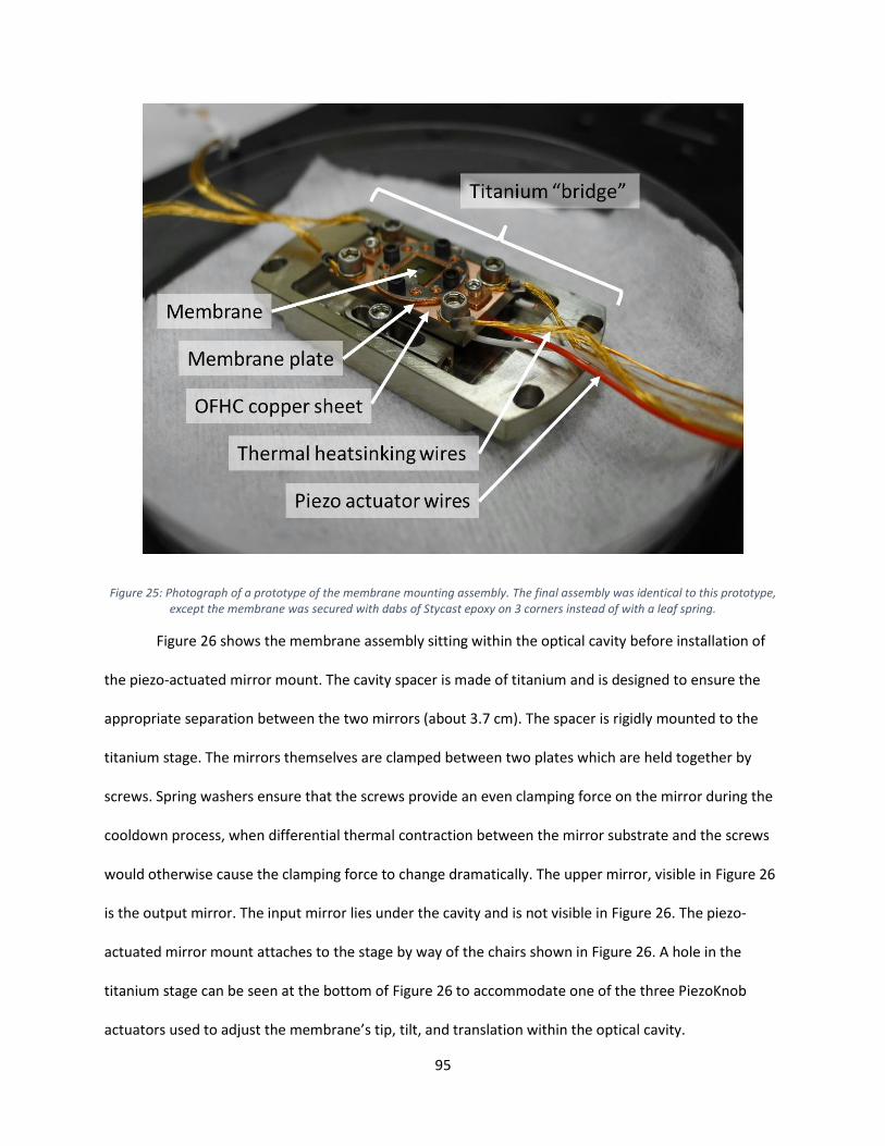
95

Figure 25: Photograph of a prototype of the membrane mounting assembly. The final assembly was identical to this prototype, except the membrane was secured with dabs of Stycast epoxy on 3 corners instead of with a leaf spring.

Figure 26 shows the membrane assembly sitting within the optical cavity before installation of

the piezo-actuated mirror mount. The cavity spacer is made of titanium and is designed to ensure the

appropriate separation between the two mirrors (about 3.7 cm). The spacer is rigidly mounted to the

titanium stage. The mirrors themselves are clamped between two plates which are held together by

screws. Spring washers ensure that the screws provide an even clamping force on the mirror during the

cooldown process, when differential thermal contraction between the mirror substrate and the screws

would otherwise cause the clamping force to change dramatically. The upper mirror, visible in Figure 26

is the output mirror. The input mirror lies under the cavity and is not visible in Figure 26. The piezo-

actuated mirror mount attaches to the stage by way of the chairs shown in Figure 26. A hole in the

titanium stage can be seen at the bottom of Figure 26 to accommodate one of the three PiezoKnob

actuators used to adjust the membrane’s tip, tilt, and translation within the optical cavity.

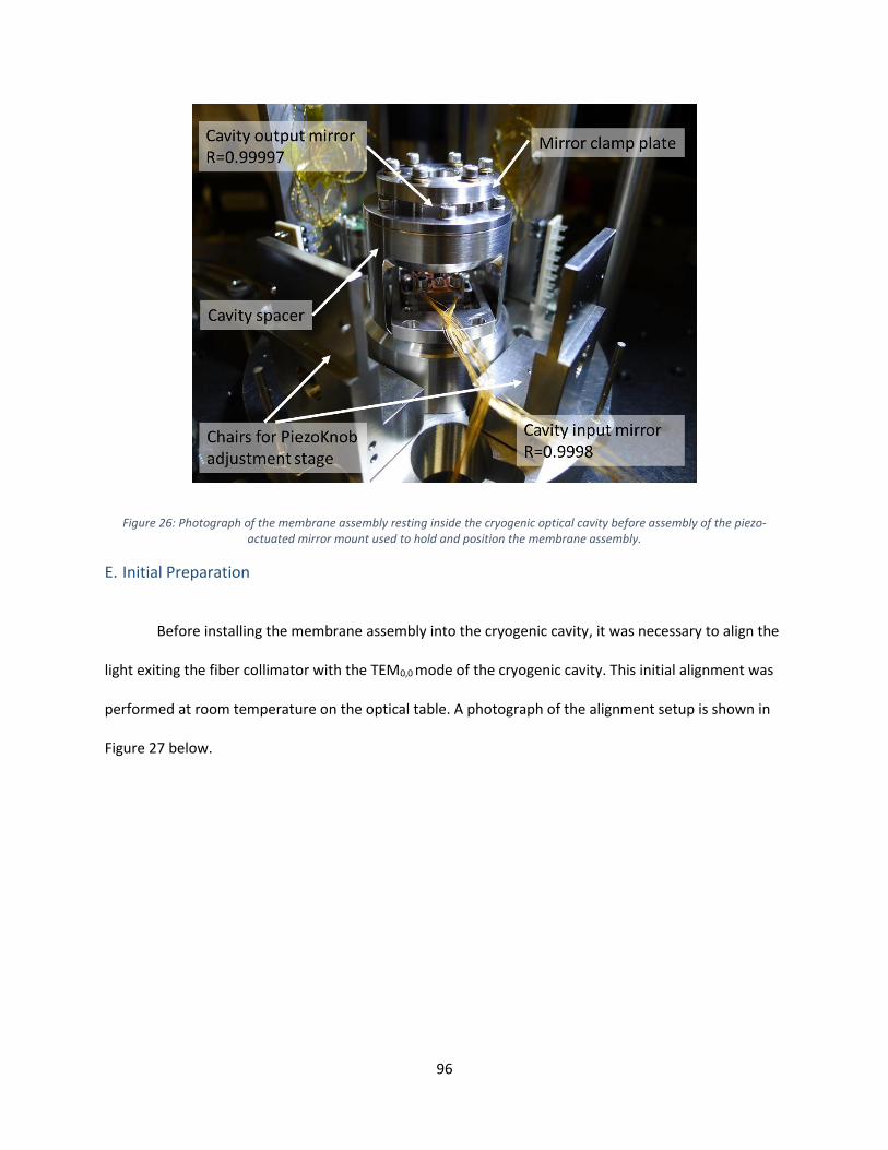
96

Figure 26: Photograph of the membrane assembly resting inside the cryogenic optical cavity before assembly of the piezo-actuated mirror mount used to hold and position the membrane assembly.

E. Initial Preparation

Before installing the membrane assembly into the cryogenic cavity, it was necessary to align the

light exiting the fiber collimator with the TEM0,0 mode of the cryogenic cavity. This initial alignment was

performed at room temperature on the optical table. A photograph of the alignment setup is shown in

Figure 27 below.

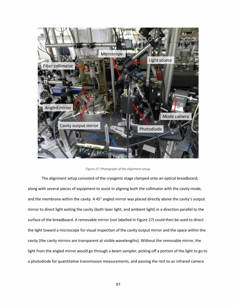
97

Figure 27: Photograph of the alignment setup.

The alignment setup consisted of the cryogenic stage clamped onto an optical breadboard,

along with several pieces of equipment to assist in aligning both the collimator with the cavity mode,

and the membrane within the cavity. A 45° angled mirror was placed directly above the cavity’s output

mirror to direct light exiting the cavity (both laser light, and ambient light) in a direction parallel to the

surface of the breadboard. A removable mirror (not labelled in Figure 27) could then be used to direct

the light toward a microscope for visual inspection of the cavity output mirror and the space within the

cavity (the cavity mirrors are transparent at visible wavelengths). Without the removable mirror, the

light from the angled mirror would go through a beam sampler, picking off a portion of the light to go to

a photodiode for quantitative transmission measurements, and passing the rest to an infrared camera

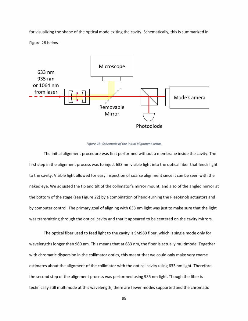
98

for visualizing the shape of the optical mode exiting the cavity. Schematically, this is summarized in

Figure 28 below.

Figure 28: Schematic of the initial alignment setup.

The initial alignment procedure was first performed without a membrane inside the cavity. The

first step in the alignment process was to inject 633 nm visible light into the optical fiber that feeds light

to the cavity. Visible light allowed for easy inspection of coarse alignment since it can be seen with the

naked eye. We adjusted the tip and tilt of the collimator’s mirror mount, and also of the angled mirror at

the bottom of the stage (see Figure 22) by a combination of hand-turning the PiezoKnob actuators and

by computer control. The primary goal of aligning with 633 nm light was just to make sure that the light

was transmitting through the optical cavity and that it appeared to be centered on the cavity mirrors.

The optical fiber used to feed light to the cavity is SM980 fiber, which is single mode only for

wavelengths longer than 980 nm. This means that at 633 nm, the fiber is actually multimode. Together

with chromatic dispersion in the collimator optics, this meant that we could only make very coarse

estimates about the alignment of the collimator with the optical cavity using 633 nm light. Therefore,

the second step of the alignment process was performed using 935 nm light. Though the fiber is

technically still multimode at this wavelength, there are fewer modes supported and the chromatic

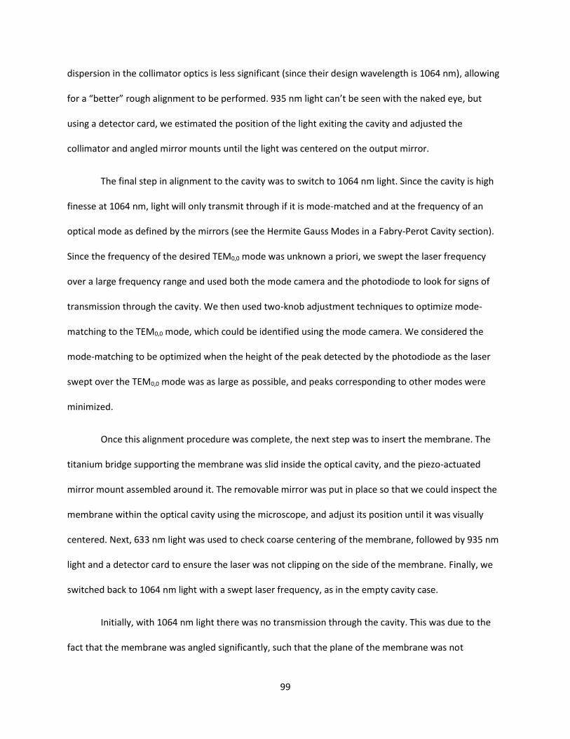
99

dispersion in the collimator optics is less significant (since their design wavelength is 1064 nm), allowing

for a “better” rough alignment to be performed. 935 nm light can’t be seen with the naked eye, but

using a detector card, we estimated the position of the light exiting the cavity and adjusted the

collimator and angled mirror mounts until the light was centered on the output mirror.

The final step in alignment to the cavity was to switch to 1064 nm light. Since the cavity is high

finesse at 1064 nm, light will only transmit through if it is mode-matched and at the frequency of an

optical mode as defined by the mirrors (see the Hermite Gauss Modes in a Fabry-Perot Cavity section).

Since the frequency of the desired TEM0,0 mode was unknown a priori, we swept the laser frequency

over a large frequency range and used both the mode camera and the photodiode to look for signs of

transmission through the cavity. We then used two-knob adjustment techniques to optimize mode-

matching to the TEM0,0 mode, which could be identified using the mode camera. We considered the

mode-matching to be optimized when the height of the peak detected by the photodiode as the laser

swept over the TEM0,0 mode was as large as possible, and peaks corresponding to other modes were

minimized.

Once this alignment procedure was complete, the next step was to insert the membrane. The

titanium bridge supporting the membrane was slid inside the optical cavity, and the piezo-actuated

mirror mount assembled around it. The removable mirror was put in place so that we could inspect the

membrane within the optical cavity using the microscope, and adjust its position until it was visually

centered. Next, 633 nm light was used to check coarse centering of the membrane, followed by 935 nm

light and a detector card to ensure the laser was not clipping on the side of the membrane. Finally, we

switched back to 1064 nm light with a swept laser frequency, as in the empty cavity case.

Initially, with 1064 nm light there was no transmission through the cavity. This was due to the

fact that the membrane was angled significantly, such that the plane of the membrane was not

100

perpendicular to the optical axis through the cavity. Though we tried to use calipers to measure the

angle of mirror mount that holds the titanium bridge of the membrane assembly relative to the base of

the stage, finding the initial alignment of the membrane to allow any transmission through the cavity at

1064 nm was largely a trial and error process. Eventually, we did notice some transmission using the

photodiode and the mode camera, and were able further adjust the membrane angle to recover

coupling to the TEM0,0 mode.

The initial cooldown of the system in the cryostat was to a temperature of 77 K using liquid

nitrogen in place of the liquid helium bath. Since liquid nitrogen is significantly less expensive than liquid

helium and also has a significantly larger heat of vaporization, it is an excellent cryogen for initial

cooling. Upon cooling the system down in the cryostat, due to uneven thermal contraction of various

parts of the stage assembly, alignment of the optics was invariably lost. We were generally able to

recover it using the same techniques described above, with slight modifications due to the fact that

once the system was inside the cryostat, we no longer had the luxury of a microscope, a photodiode

sensitive at 1064 nm, and a mode camera to help with alignment. Instead, we only had the germanium

transmission photodiode, which as discussed earlier, was not sensitive to 1064 nm light. The first step to

realigning after cooling was therefore to use the 935 nm laser to ensure that the laser was not clipping

on the frame of the membrane. To do this, we systematically stepped one of the collimator’s PiezoKnob

motors while recording transmission of 935 nm light using the transmission diode at each step. We

swept over the full range within which there was detectable transmission and eventually stopped near

the center of the transmission plateau. We then repeated this with the PiezoKnob that controlled the

orthogonal degree of freedom. The transmission as a function of the PiezoKnob’s linear displacement

(calibrated by the PiezoKnob’s response to various drive signals at room temperature) for one of these

knobs resembled the following:

101

Figure 29: Plot of 935 nm light transmission measured by the germanium photodiode as a function of linear displacement of one of the collimator PiezoKnobs.

In Figure 29, some displacements were measured more than once, and did not yield the same

amount of transmission with each measurement. From this we inferred that there is some non-

reproducibility in the motion of the PiezoKnobs, and therefore the “Displacement” may have some

random errors in addition to systematic errors caused by the change in PiezoKnob response from room

temperature to 77 K. Nonetheless, this measurement allowed us to maneuver the collimator such that

the 935 nm light was roughly centered on the membrane.

Once we were confident that the angle of the light exiting from the collimator was

approximately correct, we switched back to 1064 nm light, sweeping the laser over a large frequency

range, just as we did at room temperature. Since the transmission diode was not sensitive to this 1064

nm light at cryogenic temperatures, we used light reflected from the cavity to look for cavity modes,

102

which manifested as “dips” in the DC level coming from the reflection photodiode as the laser frequency

swept over a cavity mode. We then used two-knob adjustment techniques with the collimator

PiezoKnobs and the 45 degree angled mirror PiezoKnobs to improve coupling to whatever modes we

could find. The identity of these modes was not known a priori.

Identifying cavity modes without using a mode camera can be quite challenging, since there is

no simple way identify a mode based exclusively on the reflection dip it produces as the laser sweeps

over the mode’s resonant frequency. However, several factors helped us to identify the unknown modes

we found after performing a cursory alignment of the optics. First, there is the fact that the TEM0,0 mode

is the only non-degenerate Hermite Gauss optical cavity mode. Though normally degenerate modes can

become non-degenerate due to symmetry breaking by the membrane, these modes will still show

roughly the same behavior as a function of membrane position, making it easier to identify them as

nearly degenerate groups. Second, since the free-space beam leaving the collimator has a Gaussian

beam shape, it is well matched with the shape of TEM0,0 mode, and will therefore couple more strongly

to the TEM0,0 (assuming good alignment) than it will to any other modes.

The process of aligning the beam with the TEM0,0 mode of the cavity was therefore an iterative

process in which we measured the behavior of the modes as a function of membrane position in

between adjustments to the piezo-actuated mirror mounts within the cryostat. During this process, we

also tried to level the membrane within the optical cavity, with a goal of making it as perpendicular as

possible to the cavity’s optical axis. We could identify how level the membrane was based on the degree

of degeneracy observed in normally degenerate modes such as the TEM0,1 and TEM1,0 modes. A perfectly

level membrane should not lift the degeneracy of such modes.

We refer to each measurement of the behavior of the cavity modes as a function of membrane

position as a “bandstructure”. This term has no physical relation to the term bandstructure used in solid

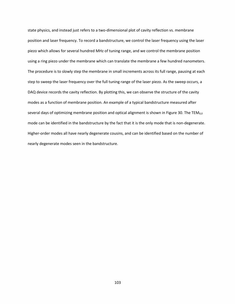
103

state physics, and instead just refers to a two-dimensional plot of cavity reflection vs. membrane

position and laser frequency. To record a bandstructure, we control the laser frequency using the laser

piezo which allows for several hundred MHz of tuning range, and we control the membrane position

using a ring piezo under the membrane which can translate the membrane a few hundred nanometers.

The procedure is to slowly step the membrane in small increments across its full range, pausing at each

step to sweep the laser frequency over the full tuning range of the laser piezo. As the sweep occurs, a

DAQ device records the cavity reflection. By plotting this, we can observe the structure of the cavity

modes as a function of membrane position. An example of a typical bandstructure measured after

several days of optimizing membrane position and optical alignment is shown in Figure 30. The TEM0,0

mode can be identified in the bandstructure by the fact that it is the only mode that is non-degenerate.

Higher-order modes all have nearly degenerate cousins, and can be identified based on the number of

nearly degenerate modes seen in the bandstructure.

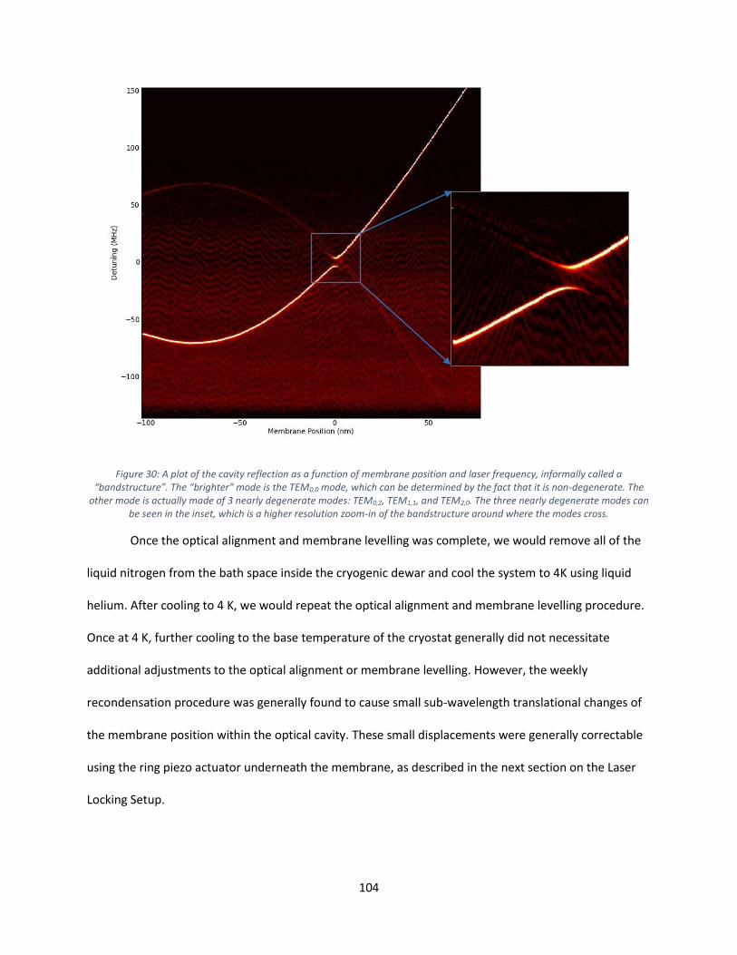
104

Figure 30: A plot of the cavity reflection as a function of membrane position and laser frequency, informally called a “bandstructure”. The “brighter” mode is the TEM0,0 mode, which can be determined by the fact that it is non-degenerate. The

other mode is actually made of 3 nearly degenerate modes: TEM0,2, TEM1,1, and TEM2,0. The three nearly degenerate modes can be seen in the inset, which is a higher resolution zoom-in of the bandstructure around where the modes cross.

Once the optical alignment and membrane levelling was complete, we would remove all of the

liquid nitrogen from the bath space inside the cryogenic dewar and cool the system to 4K using liquid

helium. After cooling to 4 K, we would repeat the optical alignment and membrane levelling procedure.

Once at 4 K, further cooling to the base temperature of the cryostat generally did not necessitate

additional adjustments to the optical alignment or membrane levelling. However, the weekly

recondensation procedure was generally found to cause small sub-wavelength translational changes of

the membrane position within the optical cavity. These small displacements were generally correctable

using the ring piezo actuator underneath the membrane, as described in the next section on the Laser

Locking Setup.

105

The final step in the preparing the system for operation was to survey several mechanical modes

of the membrane to determine which would be most suitable for ground state cooling. We did this by

measuring the mechanical quality factor and optomechanical coupling of each mode. The mechanical

quality factor was measured by mechanical ringdown, and the optomechanical coupling was estimated

by fitting measurements of the optical spring and damping using Equations (63) and (64). Unfortunately,

between the time this initial survey of modes was taken and the time the results of the experiment were

published 11, the trustworthiness of the results from this initial survey was called into question due to a

combination of technical problems with the 935 nm laser used for mechanical ringdowns, unusual

results when trying to reproduce these ringdowns, and questions over exactly how much laser power

was used in measurements of optomechanical coupling. I therefore will not discuss at length how these

measurements were performed. In spite of the questions about these results, they indicated that the

(2,2) mechanical mode at 705 kHz was the most promising for ground state cooling due to a high

mechanical quality factor and strong optomechanical coupling relative to other modes. A much more

careful measurement of mechanical quality factor and optomechanical coupling of this mode is

presented in the Data Analysis->Characterizing Parameters section.

F. Laser Locking Setup

There are many servo feedback loops used to keep the lasers and cavities on resonance with

each other or when appropriate, detuned from each other. In this section I will describe these locking

setups.

The first step in any measurement we make is to find where the membrane is within the cavity.

For this process, the classical noise performance of the lasers is not critical, so we bypass both of the

filter cavities for convenience. For ground state cooling, we ideally want the membrane positioned at a

point where the optomechanical coupling is maximized, i.e. at a point where the slope of the cavity’s

106

resonant frequency as a function of membrane position is maximized. We find the coarse position of the

membrane relative to this point by measuring the cavity bandstructure. We then identify the TEM0,0

mode and note where the node and/or anti-node of the mode is in the bandstructure. By positioning

the membrane halfway between the node and anti-node, we know that the membrane is close to the

point of maximum slope. For example, in Figure 30 the antinode of the TEM0,0 mode occurs at a

membrane position of about -75 nm (the offset of the x-axis in this figure is arbitrary). Therefore, we

expect the point of maximum linearity of the TEM0,0 mode to occur at a membrane position of +58 nm

(𝜆/8 away from the antinode).

Once the approximate point of maximum slope has been found, we move the membrane to this

point and lock the measurement laser to the cavity resonance using a Pound-Drever-Hall technique.

Optical phase modulation sidebands from the EOM (see Figure 16) are detected by the measurement

photodiode and go through a mixing circuit to produce a Pound-Drever-Hall error signal. The mixing

circuit is shown in Figure 31.

Figure 31: Block diagram of electrical circuit for locking the measurement laser to the optical cavity.

107

The error signal is fed to a PI controller (New Focus LB1005) which adjusts the tuning voltage of

a voltage controlled oscillator (Crystek CRBV55FL-0183-0219) which, after amplification through a high

power amplifier (Minicircuits ZHL-5W-1), drives AOM2. In this way, the frequency of the measurement

laser can be kept on resonance with the optical cavity. The frequency shifting range of AOM2 is

approximately 200 MHz ± ~100 MHz. However, the diffraction efficiency of AOM2 drops as the deviation

from 200 MHz gets larger. Therefore a second PI controller takes the output of the first PI controller as

its error signal and sends feedback to the laser piezo of the measurement laser. This feedback is low-

passed at several Hz, and is primarily intended to keep the drive frequency of AOM2 centered near 200

MHz. A portion of this signal also gets split off to feed forward to FC1, which will be discussed in a bit.

Once the probe beam has been locked to the cavity, the next step is to lock the cooling laser to

the measurement laser with an offset equal to approximately two free spectral ranges of the cold cavity.

This is done for several reasons: (1) since the cooling laser is typically detuned from the cavity resonance

by an amount comparable to 𝜔𝑚, coupling the laser to a different longitudinal mode several GHz away

prevents the formation of a beat note at 𝜔𝑚 inside the cavity, and (2) the slope of the linear region of

the cavity resonance as a function of membrane position has a sign which alternates with each free

spectral range – therefore to keep both lasers in a region with the same sign, it is necessary to detune

the cooling laser by two free spectral ranges. It is important that the two modes have the same sign

because the measurement and cooling beams both receive the same frequency shifts from AOM2. If the

beams are coupling to modes which have different slopes as a function of membrane position, then only

one of the two beams will receive the necessary frequency shifts from AOM2 to track the cavity’s

resonance – the other will receive frequency shifts that are the opposite of the actual fluctuations of the

mode it is coupled to.

To actually perform the offset lock, a scheme similar to the one described in Ref. [ 55] is

employed. As shown in Figure 16, a portion of both the measurement and cooling lasers are picked off

108

right after light exits the lasers themselves and combined on a photodiode. This photodiode is a

Newport Model 1554-B, which has a 12 GHz bandwidth and is therefore able to directly detect the ~8

GHz optical beat note between the two lasers. The output of this photodiode is sent into a high

frequency mixer, where it is combined with a reference tone from a Rohde & Schwartz signal generator.

When the frequency of the optical beat note and the reference tone are near each other, the output of

the high frequency mixer has frequency components near DC and near 16 GHz. The 16 GHz component

is suppressed due to the bandwidth of the mixer. The component near DC has a frequency which

represents the offset in frequency between the optical beat note and the reference tone from the signal

generator. To produce an error signal for servo feedback to keep the frequency offset locked, it is

necessary to convert the frequency of this signal into a voltage. This is easily done by mixing it with a

low-passed version of itself, where the low-pass corner frequency is selected so that there is a steep

linear roll-off of phase around the desired frequency offset. We do this using a Minicircuits BLP-1.9+ low

pass filter which has a 3 dB corner frequency of 2.5MHz. (The frequency dependent phase shift from this

filter replaces the phase shift introduced by the coaxial delay line in Ref. [ 55].) The phase shift

introduced by this filter makes it so that after mixing the low passed and non-low passed signals, there is

a component at DC corresponding to the error in frequency between the optical beat note and the

reference tone. The other component at a few MHz is filtered out with a second BLP-1.9+ filter. The DC

component is fed into a New Focus LB1005 servo controller, and the output of that controller is sent to

the laser piezo of the cooling laser to keep it locked with the appropriate offset. A schematic of this

setup is shown in Figure 32.

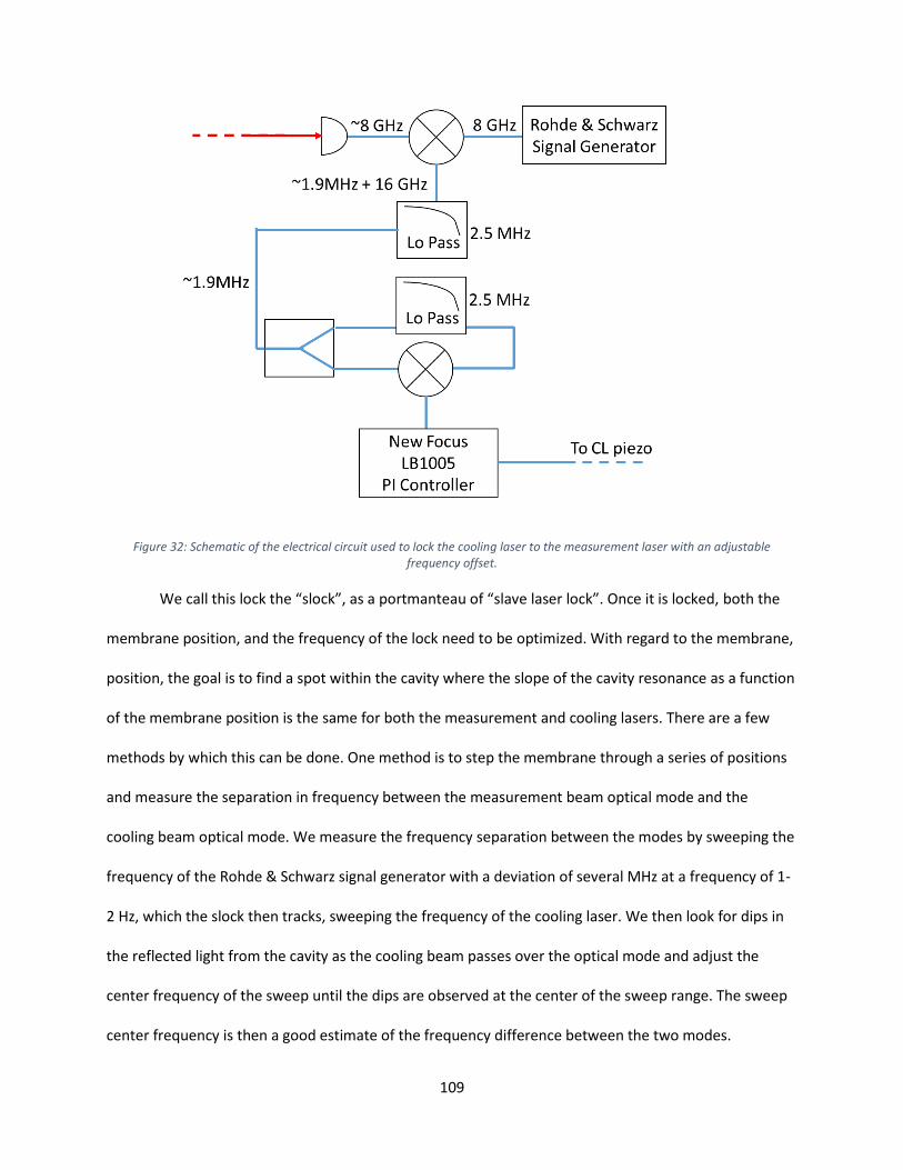
109

Figure 32: Schematic of the electrical circuit used to lock the cooling laser to the measurement laser with an adjustable frequency offset.

We call this lock the “slock”, as a portmanteau of “slave laser lock”. Once it is locked, both the

membrane position, and the frequency of the lock need to be optimized. With regard to the membrane,

position, the goal is to find a spot within the cavity where the slope of the cavity resonance as a function

of the membrane position is the same for both the measurement and cooling lasers. There are a few

methods by which this can be done. One method is to step the membrane through a series of positions

and measure the separation in frequency between the measurement beam optical mode and the

cooling beam optical mode. We measure the frequency separation between the modes by sweeping the

frequency of the Rohde & Schwarz signal generator with a deviation of several MHz at a frequency of 1-

2 Hz, which the slock then tracks, sweeping the frequency of the cooling laser. We then look for dips in

the reflected light from the cavity as the cooling beam passes over the optical mode and adjust the

center frequency of the sweep until the dips are observed at the center of the sweep range. The sweep

center frequency is then a good estimate of the frequency difference between the two modes.

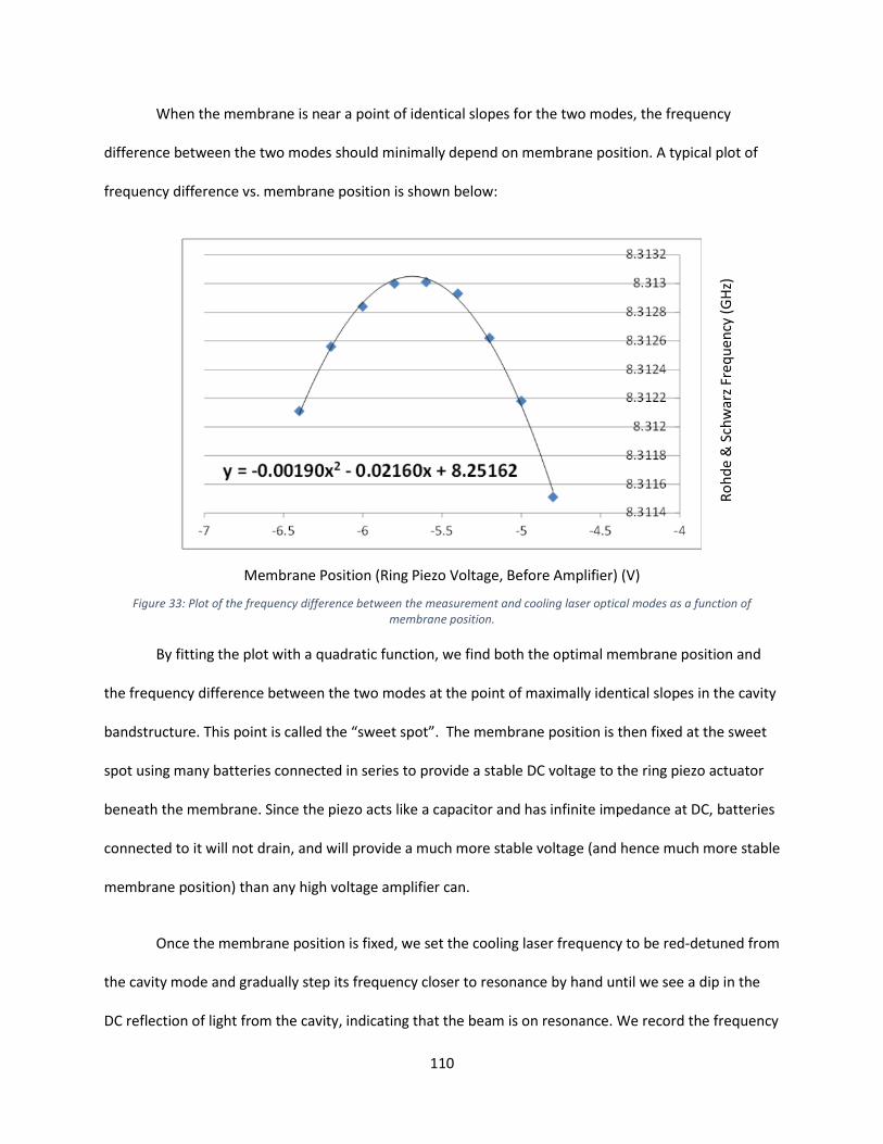
110

When the membrane is near a point of identical slopes for the two modes, the frequency

difference between the two modes should minimally depend on membrane position. A typical plot of

frequency difference vs. membrane position is shown below:

Figure 33: Plot of the frequency difference between the measurement and cooling laser optical modes as a function of membrane position.

By fitting the plot with a quadratic function, we find both the optimal membrane position and

the frequency difference between the two modes at the point of maximally identical slopes in the cavity

bandstructure. This point is called the “sweet spot”. The membrane position is then fixed at the sweet

spot using many batteries connected in series to provide a stable DC voltage to the ring piezo actuator

beneath the membrane. Since the piezo acts like a capacitor and has infinite impedance at DC, batteries

connected to it will not drain, and will provide a much more stable voltage (and hence much more stable

membrane position) than any high voltage amplifier can.

Once the membrane position is fixed, we set the cooling laser frequency to be red-detuned from

the cavity mode and gradually step its frequency closer to resonance by hand until we see a dip in the

DC reflection of light from the cavity, indicating that the beam is on resonance. We record the frequency

Ro

hd

e &

Sch

war

z Fr

equ

ency

(G

Hz)

Membrane Position (Ring Piezo Voltage, Before Amplifier) (V)

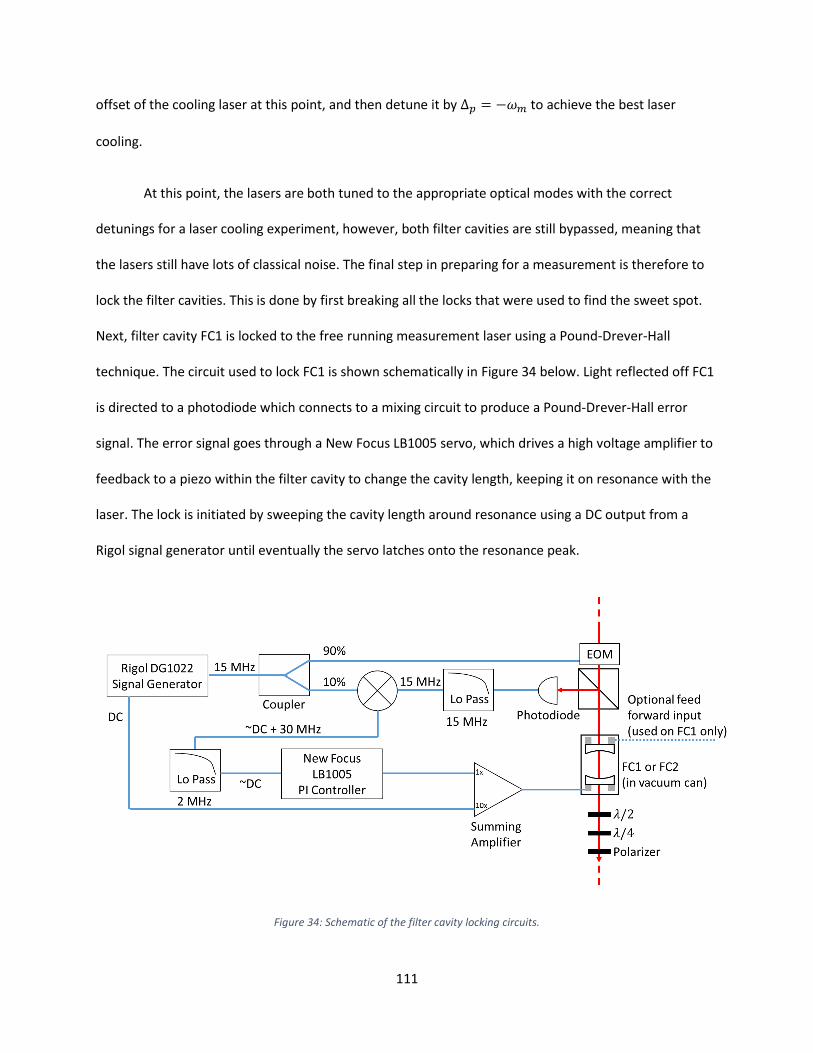
111

offset of the cooling laser at this point, and then detune it by Δ𝑝 = −𝜔𝑚 to achieve the best laser

cooling.

At this point, the lasers are both tuned to the appropriate optical modes with the correct

detunings for a laser cooling experiment, however, both filter cavities are still bypassed, meaning that

the lasers still have lots of classical noise. The final step in preparing for a measurement is therefore to

lock the filter cavities. This is done by first breaking all the locks that were used to find the sweet spot.

Next, filter cavity FC1 is locked to the free running measurement laser using a Pound-Drever-Hall

technique. The circuit used to lock FC1 is shown schematically in Figure 34 below. Light reflected off FC1

is directed to a photodiode which connects to a mixing circuit to produce a Pound-Drever-Hall error

signal. The error signal goes through a New Focus LB1005 servo, which drives a high voltage amplifier to

feedback to a piezo within the filter cavity to change the cavity length, keeping it on resonance with the

laser. The lock is initiated by sweeping the cavity length around resonance using a DC output from a

Rigol signal generator until eventually the servo latches onto the resonance peak.

Figure 34: Schematic of the filter cavity locking circuits.

112

Once FC1 is locked, it is necessary to lock to the cold cavity again. Since the laser was previously

locked to the optical mode of the cryogenic cavity before locking FC1, it is typically still close to

resonance, and can be locked just by sweeping the drive frequency of AOM2. On occasion, if things have

drifted, it is necessary to make slow adjustments to the measurement laser frequency using the

measurement laser’s piezo. These adjustments must be made very slowly so that FC1 can track the

changes in frequency without unlocking. This is where feeding forward a portion of the ML piezo drive

signal to FC1 is helpful, as it reduces the work that must be done by the PDH lock to track changes to the

measurement laser frequency. Details of how the feed forward scheme works and the requirements

necessary to implement it are described in Ref. [ 41].

Once the measurement laser has been locked to the cold cavity, the slock is relocked as already

described at the optimal frequency for laser cooling, and then filter cavity FC2 is locked to the cooling

laser. Now, since all the laser beams pass through AOM2 before reaching the cold cavity, they all track

fluctuations of the cold cavity and stay appropriately on resonance with, or detuned from, the cavity

modes. At this point it is possible to start measuring the behavior of the membrane as it is cooled by the

laser.

4. Measuring the Membrane’s Motion

As shown in Figure 17, the light reflected from the cryogenic cavity has several different

frequency components. When these land on the measurement photodiode, interference between these

components produces beat notes in the photocurrent at the sum and difference frequencies between all

the components, as shown in Figure 18. The beat note between the local oscillator and the

measurement beam and its mechanical sidebands produces components in the photocurrent at

80 MHz ± 705 kHz. The circuit we use to isolate and record these components works as follows. The

signal from the photodiode first goes through a bias tee to separate the DC level from the RF

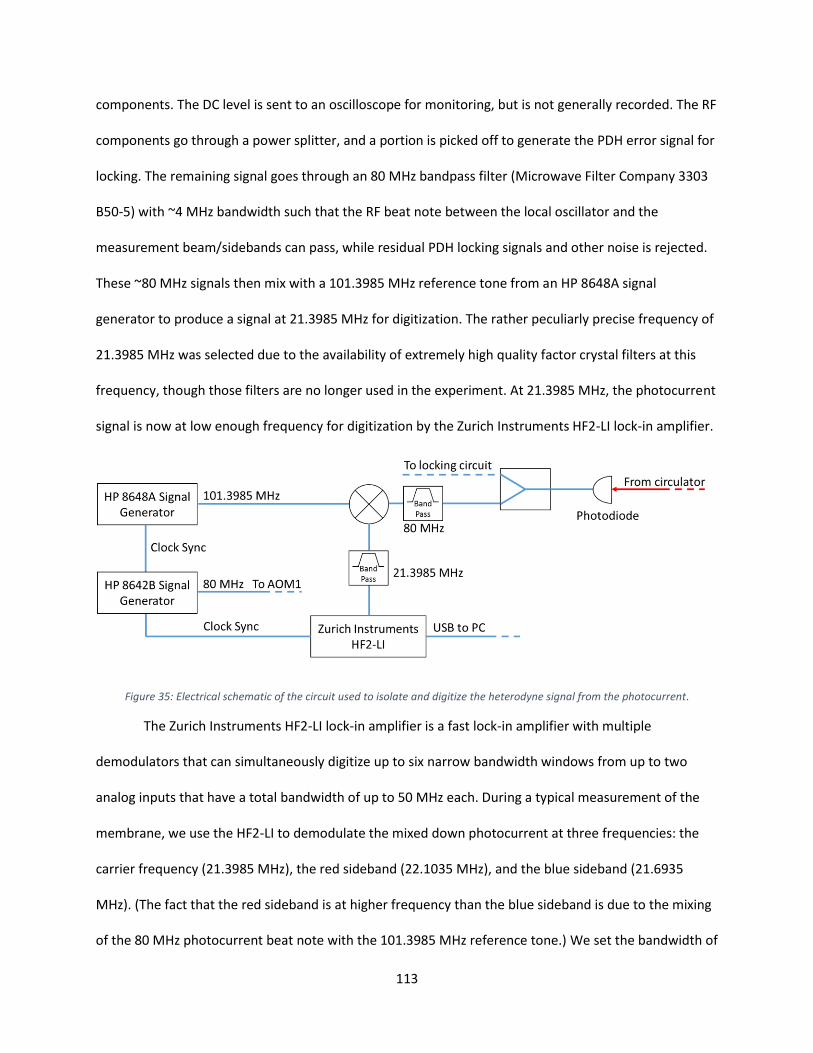
113

components. The DC level is sent to an oscilloscope for monitoring, but is not generally recorded. The RF

components go through a power splitter, and a portion is picked off to generate the PDH error signal for

locking. The remaining signal goes through an 80 MHz bandpass filter (Microwave Filter Company 3303

B50-5) with ~4 MHz bandwidth such that the RF beat note between the local oscillator and the

measurement beam/sidebands can pass, while residual PDH locking signals and other noise is rejected.

These ~80 MHz signals then mix with a 101.3985 MHz reference tone from an HP 8648A signal

generator to produce a signal at 21.3985 MHz for digitization. The rather peculiarly precise frequency of

21.3985 MHz was selected due to the availability of extremely high quality factor crystal filters at this

frequency, though those filters are no longer used in the experiment. At 21.3985 MHz, the photocurrent

signal is now at low enough frequency for digitization by the Zurich Instruments HF2-LI lock-in amplifier.

Figure 35: Electrical schematic of the circuit used to isolate and digitize the heterodyne signal from the photocurrent.

The Zurich Instruments HF2-LI lock-in amplifier is a fast lock-in amplifier with multiple

demodulators that can simultaneously digitize up to six narrow bandwidth windows from up to two

analog inputs that have a total bandwidth of up to 50 MHz each. During a typical measurement of the

membrane, we use the HF2-LI to demodulate the mixed down photocurrent at three frequencies: the

carrier frequency (21.3985 MHz), the red sideband (22.1035 MHz), and the blue sideband (21.6935

MHz). (The fact that the red sideband is at higher frequency than the blue sideband is due to the mixing

of the 80 MHz photocurrent beat note with the 101.3985 MHz reference tone.) We set the bandwidth of

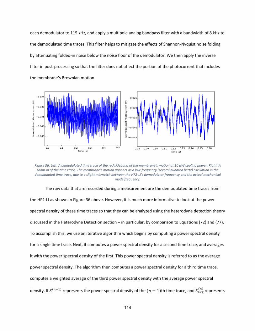
114

each demodulator to 115 kHz, and apply a multipole analog bandpass filter with a bandwidth of 8 kHz to

the demodulated time traces. This filter helps to mitigate the effects of Shannon-Nyquist noise folding

by attenuating folded-in noise below the noise floor of the demodulator. We then apply the inverse

filter in post-processing so that the filter does not affect the portion of the photocurrent that includes

the membrane’s Brownian motion.

Figure 36: Left: A demodulated time trace of the red sideband of the membrane’s motion at 10 µW cooling power. Right: A zoom-in of the time trace. The membrane’s motion appears as a low-frequency (several hundred hertz) oscillation in the

demodulated time trace, due to a slight mismatch between the HF2-LI’s demodulator frequency and the actual mechanical mode frequency.

The raw data that are recorded during a measurement are the demodulated time traces from

the HF2-LI as shown in Figure 36 above. However, it is much more informative to look at the power

spectral density of these time traces so that they can be analyzed using the heterodyne detection theory

discussed in the Heterodyne Detection section – in particular, by comparison to Equations (72) and (77).

To accomplish this, we use an iterative algorithm which begins by computing a power spectral density

for a single time trace. Next, it computes a power spectral density for a second time trace, and averages

it with the power spectral density of the first. This power spectral density is referred to as the average

power spectral density. The algorithm then computes a power spectral density for a third time trace,

computes a weighted average of the third power spectral density with the average power spectral

density. If 𝑆(𝑛+1) represents the power spectral density of the (𝑛 + 1)th time trace, and 𝑆avg(𝑛) represents

115

the average power spectral density after 𝑛 time traces, the following recursion relation describes how

the average power spectral density is computed:

𝑆avg(𝑛+1)

=𝑛𝑆avg

(𝑛)+ 𝑆(𝑛+1)

𝑛 + 1 (84)

Using a recursive process to combine separate power spectral densities into an average power

spectral density is convenient for several reasons. First, it allows for real time display of the power

spectral density while collecting data. Second, it allows for computation of a power spectral density

representing, potentially, hours of data, without the need to Fourier transform an hours-long time trace.

Since the length of the time trace used to compute any individual Fourier transform or power spectral

density determines the spectral resolution, we set the length of our time traces to 0.5 seconds, which

corresponds to a resolution of 2 Hz. An hours-long time trace would produce a spectrum with millihertz

resolution which could then be binned to 2 Hz to reduce noise, but would be more computationally

complex to achieve, and would not allow for real-time viewing of the power spectral density.

For a laser cooling measurement, a typical measurement involves collecting sufficiently many

time traces at each cooling laser power to clearly resolve the shape of the Brownian motion above the

fuzz in the noise floor in the real time power spectral density. At low cooling powers, the Brownian

motion is very large, and can be resolved after only a few dozen 0.5 second time traces. In practice, for

the best data, we typically collect far more time traces than are actually needed to resolve the motion

above the fuzz, so a low cooling power measurement might have an average PSD computed from on the

order of 100 time traces. With a time trace length of 0.5 seconds, this represents a total data length of

under a minute, which can be collected (after accounting for overhead in data acquisition) in 1-2

minutes. Figure 37 shows a typical low cooling power power spectral density.

116

Figure 37: Typical average power spectral density of one sideband of the membrane’s motion at a cooling power of 10 uW. This power spectral density was produced using 102 time traces of 0.5 seconds each.

At the highest cooling powers, the Brownian motion is heavily damped and has a much smaller

amplitude that is on the order of the size of the fuzz in Figure 37. In order to resolve the Brownian

motion in the power spectral density when it is so heavily damped, it is necessary to collect drastically

more time traces than at low cooling power. Since the fuzz in the power spectral density is assumed to

be Gaussian distributed, its standard deviation should become smaller like the square root of the

number of time traces that were used to compute the average power spectrum. Therefore, after

averaging ten times more time traces, the fuzz gets smaller only by a factor of about 3.2. The longest

practical measurement we can make (due to stability concerns, and the fact that humans eventually get

tired), is on the order of several hours, or tens of thousands of seconds, and therefore achieving even an

order of magnitude reduction in the size of the fuzz by collecting more data is difficult. However, since

the heavily damped motion of the oscillator at high cooling powers can have linewidths of several

117

kilohertz, we are able to trade some spectral resolution in exchange for reduced fuzz by binning

together adjacent points in the average power spectral density. Since our spectral resolution is 2 Hz and

the linewidth of the Brownian motion is several kilohertz, selecting a bin size of 20 Hz (10x the original

spectral resolution), for example, has no negative effect on the Brownian motion in the power

spectrum, but reduces the fuzz in a way equivalent to if we measured 10x longer than we actually did.

Therefore, a combination of long measurements and appropriate binning are used to produce good

power spectral densities of data taken at high cooling powers. Figure 38 shows an example of the

reduction in fuzz that can be achieved by binning from a spectral resolution of 2 Hz to a spectral

resolution of 20 Hz as described above. (The ostensibly larger-than-3.2x reduction in the fuzz is an

artifact of trying to display such a high spectral resolution in the left plot – relatively infrequent large

deviations from the mean are smooshed together in the plot due to the limited resolution of the screen

or printer from which you are reading this, making the fuzz seem larger. Nonetheless, the reduction in

fuzz is still dramatic.) By looking at the real-time power spectral density as we collect the data and

adjusting the bin size as needed, we are able to estimate when we have collected enough time traces for

a given measurement.

Figure 38: Left, an average power spectral density of the membrane’s motion at 450 uW cooling power computed from 1,302 time traces (651 seconds of data). Right, the same average power spectral density after binning to reduce the spectral resolution by a factor of 10, in exchange for reducing the fuzz as if the power spectral density was computed from 13,020 time traces (6510

seconds of data).

118

5. Data Analysis

A. First Steps

After collecting an adequate number of time traces at each cooling laser power we begin data

analysis of the average power spectral densities. While the power spectral densities are completely

described by Equations (72), (77), and (81), we typically begin analysis by fitting the power spectral

densities to a generic Lorentzian form. Using a generic Lorentzian instead of the full equations for the

power spectral densities is a good first step in analysis because it is possible to extract the basic behavior

of the mechanical mode without the need to carefully calibrate each parameter in Equations (72), (77),

and (81). Fitting to just a Lorentzian rather than a Fano lineshape assumes that 𝐴𝑟𝑟 and 𝐴𝑏𝑏 are

negligibly small compared with, 𝐿𝑟𝑟 and 𝐿𝑏𝑏, and 𝐹𝑟𝑟 and 𝐹𝑏𝑏 respectively. This is a valid assumption in

the limit of small classical laser noise on the measurement beam – an assumption which I will revisit

later in the section Characterizing Parameters->Classical Laser Noise.

Before fitting the data, we first subtract the heterodyne carrier frequency from the x-axis such

that the red sideband occurs at +705 kHz, and the blue sideband at -705 kHz. We then reflect the blue

sideband about zero frequency for easier visual comparison with the red sideband, and scale the x-axis

of both sidebands into units of kilohertz. The Lorentzian fits to the data are then simultaneously

performed for the red and the blue sidebands. The form of the fits are:

{

𝑆𝑟𝑟 = 𝑏𝑟𝑟 +

𝑠𝑟𝑟

1 + (𝑓 − 𝑓𝑐𝑓ℎ

)2

𝑆𝑏𝑏 = 𝑏𝑏𝑏 +𝑠𝑏𝑏

1 + (𝑓 − 𝑓𝑐𝑓ℎ

)2

(85)

The red and the blue sidebands are each allowed to have different noise backgrounds 𝑏𝑟𝑟 and

𝑏𝑏𝑏. This is because dispersion in the dark noise and gain of the photodiode/mixing circuit can cause the

noise backgrounds of each sideband to differ. The amplitudes of the Lorentzian peaks, 𝑠𝑟𝑟 and 𝑠𝑏𝑏, are

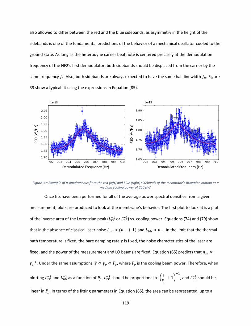
119

also allowed to differ between the red and the blue sidebands, as asymmetry in the height of the

sidebands is one of the fundamental predictions of the behavior of a mechanical oscillator cooled to the

ground state. As long as the heterodyne carrier beat note is centered precisely at the demodulation

frequency of the HF2’s first demodulator, both sidebands should be displaced from the carrier by the

same frequency 𝑓𝑐. Also, both sidebands are always expected to have the same half linewidth 𝑓ℎ. Figure

39 show a typical fit using the expressions in Equation (85).

Figure 39: Example of a simultaneous fit to the red (left) and blue (right) sidebands of the membrane’s Brownian motion at a medium cooling power of 250 µW.

Once fits have been performed for all of the average power spectral densities from a given

measurement, plots are produced to look at the membrane’s behavior. The first plot to look at is a plot

of the inverse area of the Lorentzian peak (𝐿𝑟𝑟−1 or 𝐿𝑏𝑏

−1) vs. cooling power. Equations (74) and (79) show

that in the absence of classical laser noise 𝐿𝑟𝑟 ∝ (𝑛𝑚 + 1) and 𝐿𝑏𝑏 ∝ 𝑛𝑚. In the limit that the thermal

bath temperature is fixed, the bare damping rate 𝛾 is fixed, the noise characteristics of the laser are

fixed, and the power of the measurement and LO beams are fixed, Equation (65) predicts that 𝑛𝑚 ∝

𝛾𝑝−1. Under the same assumptions, �� ∝ 𝛾𝑝 ∝ 𝑃𝑝, where 𝑃𝑝 is the cooling beam power. Therefore, when

plotting 𝐿𝑟𝑟−1 and 𝐿𝑏𝑏

−1 as a function of 𝑃𝑝, 𝐿𝑟𝑟−1 should be proportional to (

1

𝑃𝑝+ 1)

−1

, and 𝐿𝑏𝑏−1 should be

linear in 𝑃𝑝. In terms of the fitting parameters in Equation (85), the area can be represented, up to a

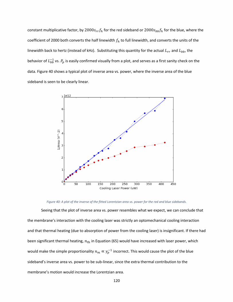
120

constant multiplicative factor, by 2000𝑠𝑟𝑟𝑓ℎ for the red sideband or 2000𝑠𝑏𝑏𝑓ℎ for the blue, where the

coefficient of 2000 both converts the half linewidth 𝑓ℎ to full linewidth, and converts the units of the

linewidth back to hertz (instead of kHz). Substituting this quantity for the actual 𝐿𝑟𝑟 and 𝐿𝑏𝑏, the

behavior of 𝐿𝑏𝑏−1 vs. 𝑃𝑝 is easily confirmed visually from a plot, and serves as a first sanity check on the

data. Figure 40 shows a typical plot of inverse area vs. power, where the inverse area of the blue

sideband is seen to be clearly linear.

Figure 40: A plot of the inverse of the fitted Lorentzian area vs. power for the red and blue sidebands.

Seeing that the plot of inverse area vs. power resembles what we expect, we can conclude that

the membrane’s interaction with the cooling laser was strictly an optomechanical cooling interaction

and that thermal heating (due to absorption of power from the cooling laser) is insignificant. If there had

been significant thermal heating, 𝑛th in Equation (65) would have increased with laser power, which

would make the simple proportionality 𝑛𝑚 ∝ 𝛾𝑝−1 incorrect. This would cause the plot of the blue

sideband’s inverse area vs. power to be sub-linear, since the extra thermal contribution to the

membrane’s motion would increase the Lorentzian area.

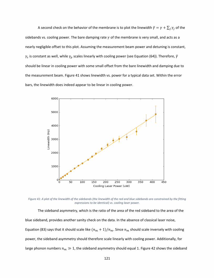
121

A second check on the behavior of the membrane is to plot the linewidth �� = 𝛾 + ∑ 𝛾𝑗𝑗 of the

sidebands vs. cooling power. The bare damping rate 𝛾 of the membrane is very small, and acts as a

nearly negligible offset to this plot. Assuming the measurement beam power and detuning is constant,

𝛾𝑠 is constant as well, while 𝛾𝑝 scales linearly with cooling power (see Equation (64)). Therefore, ��

should be linear in cooling power with some small offset from the bare linewidth and damping due to

the measurement beam. Figure 41 shows linewidth vs. power for a typical data set. Within the error

bars, the linewidth does indeed appear to be linear in cooling power.

Figure 41: A plot of the linewidth of the sidebands (the linewidth of the red and blue sidebands are constrained by the fitting expressions to be identical) vs. cooling laser power.

The sideband asymmetry, which is the ratio of the area of the red sideband to the area of the

blue sideband, provides another sanity check on the data. In the absence of classical laser noise,

Equation (83) says that it should scale like (𝑛𝑚 + 1)/𝑛𝑚. Since 𝑛𝑚 should scale inversely with cooling

power, the sideband asymmetry should therefore scale linearly with cooling power. Additionally, for

large phonon numbers 𝑛𝑚 ≫ 1, the sideband asymmetry should equal 1. Figure 42 shows the sideband

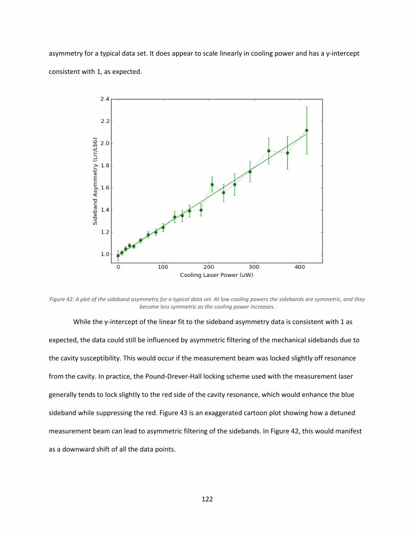
122

asymmetry for a typical data set. It does appear to scale linearly in cooling power and has a y-intercept

consistent with 1, as expected.

Figure 42: A plot of the sideband asymmetry for a typical data set. At low cooling powers the sidebands are symmetric, and they become less symmetric as the cooling power increases.

While the y-intercept of the linear fit to the sideband asymmetry data is consistent with 1 as

expected, the data could still be influenced by asymmetric filtering of the mechanical sidebands due to

the cavity susceptibility. This would occur if the measurement beam was locked slightly off resonance

from the cavity. In practice, the Pound-Drever-Hall locking scheme used with the measurement laser

generally tends to lock slightly to the red side of the cavity resonance, which would enhance the blue

sideband while suppressing the red. Figure 43 is an exaggerated cartoon plot showing how a detuned

measurement beam can lead to asymmetric filtering of the sidebands. In Figure 42, this would manifest

as a downward shift of all the data points.

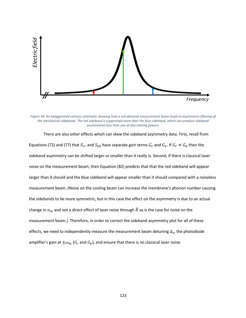
123

Figure 43: An exaggerated cartoon schematic showing how a red-detuned measurement beam leads to asymmetric filtering of the mechanical sidebands. The red sideband is suppressed more than the blue sideband, which can produce sideband

asymmetries less than one at low cooling powers.

There are also other effects which can skew the sideband asymmetry data. First, recall from

Equations (72) and (77) that 𝑆𝑟𝑟 and 𝑆𝑏𝑏 have separate gain terms 𝐺𝑟 and 𝐺𝑏. If 𝐺𝑟 ≠ 𝐺𝑏 then the

sideband asymmetry can be shifted larger or smaller than it really is. Second, if there is classical laser

noise on the measurement beam, then Equation (82) predicts that that the red sideband will appear

larger than it should and the blue sideband will appear smaller than it should compared with a noiseless

measurement beam. (Noise on the cooling beam can increase the membrane’s phonon number causing

the sidebands to be more symmetric, but in this case the effect on the asymmetry is due to an actual

change in 𝑛𝑚 and not a direct effect of laser noise through �� as is the case for noise on the

measurement beam.) Therefore, in order to correct the sideband asymmetry plot for all of these

effects, we need to independently measure the measurement beam detuning Δ𝑠, the photodiode

amplifier’s gain at ±𝜔𝑚 (𝐺𝑟 and 𝐺𝑏), and ensure that there is no classical laser noise.

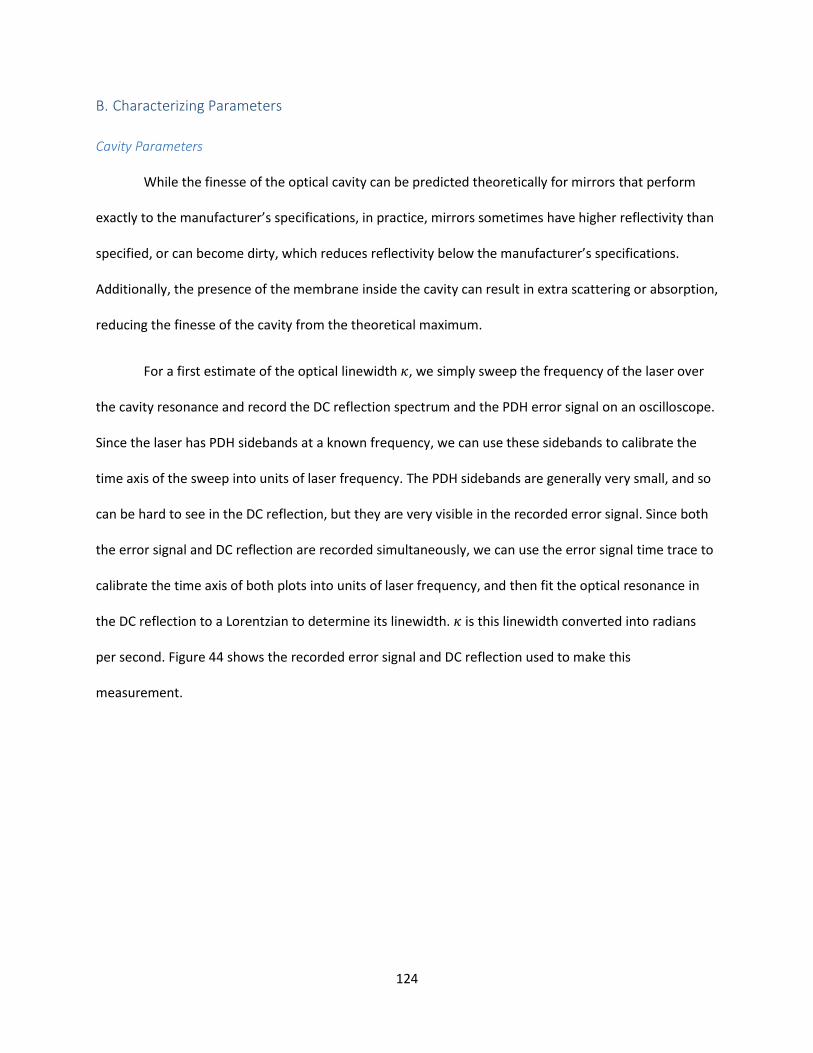
124

B. Characterizing Parameters

Cavity Parameters

While the finesse of the optical cavity can be predicted theoretically for mirrors that perform

exactly to the manufacturer’s specifications, in practice, mirrors sometimes have higher reflectivity than

specified, or can become dirty, which reduces reflectivity below the manufacturer’s specifications.

Additionally, the presence of the membrane inside the cavity can result in extra scattering or absorption,

reducing the finesse of the cavity from the theoretical maximum.

For a first estimate of the optical linewidth 𝜅, we simply sweep the frequency of the laser over

the cavity resonance and record the DC reflection spectrum and the PDH error signal on an oscilloscope.

Since the laser has PDH sidebands at a known frequency, we can use these sidebands to calibrate the

time axis of the sweep into units of laser frequency. The PDH sidebands are generally very small, and so

can be hard to see in the DC reflection, but they are very visible in the recorded error signal. Since both

the error signal and DC reflection are recorded simultaneously, we can use the error signal time trace to

calibrate the time axis of both plots into units of laser frequency, and then fit the optical resonance in

the DC reflection to a Lorentzian to determine its linewidth. 𝜅 is this linewidth converted into radians

per second. Figure 44 shows the recorded error signal and DC reflection used to make this

measurement.

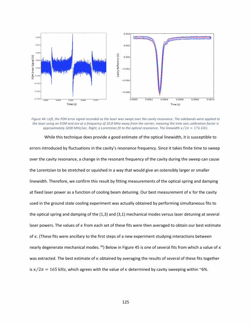
125

Figure 44: Left, the PDH error signal recorded as the laser was swept over the cavity resonance. The sidebands were applied to the laser using an EOM and are at a frequency of 10.8 MHz away from the carrier, meaning the time axis calibration factor is

approximately 3200 MHz/sec. Right, a Lorentzian fit to the optical resonance. The linewidth 𝜅 2𝜋⁄ ≈ 176 𝑘𝐻𝑧.

While this technique does provide a good estimate of the optical linewidth, it is susceptible to

errors introduced by fluctuations in the cavity’s resonance frequency. Since it takes finite time to sweep

over the cavity resonance, a change in the resonant frequency of the cavity during the sweep can cause

the Lorentzian to be stretched or squished in a way that would give an ostensibly larger or smaller

linewidth. Therefore, we confirm this result by fitting measurements of the optical spring and damping

at fixed laser power as a function of cooling beam detuning. Our best measurement of 𝜅 for the cavity

used in the ground state cooling experiment was actually obtained by performing simultaneous fits to

the optical spring and damping of the (1,3) and (3,1) mechanical modes versus laser detuning at several

laser powers. The values of 𝜅 from each set of these fits were then averaged to obtain our best estimate

of 𝜅. (These fits were ancillary to the first steps of a new experiment studying interactions between

nearly degenerate mechanical modes. 56) Below in Figure 45 is one of several fits from which a value of 𝜅

was extracted. The best estimate of 𝜅 obtained by averaging the results of several of these fits together

is 𝜅 2𝜋⁄ = 165 kHz, which agrees with the value of 𝜅 determined by cavity sweeping within ~6%.

126

Figure 45: Simultaneous fits to the optical spring and damping of the (1,3) and (3,1) modes to obtain 𝜅.

𝜅in is the cavity parameter which characterizes the transmission through the mirrors of the

optical cavity. Recalling from Equation (68) the expression for the normalized amplitude of the reflected

field after the laser’s interaction with the cavity, 𝜌(Δ) = 𝛽 −𝜅in

𝜅 2⁄ +𝑖Δ, it is possible to solve for 𝜅ext using

the measured value of 𝜅 and the value of 𝛽 which shall be discussed in the next section. Precisely on

resonance, Δ = 0, and 𝜌(0) = 𝛽 − 2𝜅in/𝜅. This can be solved for 𝜅in =𝜅

2(𝛽 − 𝜌(0)). By this method

we find 𝜅in 2𝜋⁄ ≈ 65 kHz.

Optical Losses and Efficiencies

Since the cooling measurement of the mechanical mode measures the mode’s behavior as a

function of cooling laser power, it is essential to know exactly how much laser power reaches the optical

cavity, how much of that power returns to the photodiode, and how much of the power reaching the

127

photodiode is actually detected. These efficiencies and losses are described by several parameters, most

of which can be independently measured. Following the circulator in Figure 16, there is a 99:1 fiber

beam splitter which is used to pick off 1% of the optical power to measure with a power meter. The

power meter is calibrated so that from the 1% output of the beam splitter, it reads the amount of power

that is actually coming out of the 99% port. The 99% port is fusion spliced onto the fiber that goes into

the fridge. The loss in this splice is one of the few losses that cannot be directly measured, but it is

estimated based on other losses as will be described.

Once in the fiber that goes into the fridge, light is assumed to pass losslessly out the fiber

collimator and then in free-space to the optical cavity. Light that reflects back from the optical cavity

recouples into the optical fiber with an efficiency which we can measure. This measurement is

performed by sending light into the fridge from free-space directly into the fridge fiber (without an

inline circulator or 99:1 beamsplitter) and measuring how much power reflects back. We then cut the

fiber and measure how much light comes out to determine the free-space-to-fiber coupling. The ratio of

the the power of the reflected light to the power of the light coming out of the cut fiber gives the fiber

recoupling efficiency inside the fridge, 𝛽2 ≈ 0.77. It should be noted that this measurement is

performed without locking the lasers to the cavity, and therefore this recoupling efficiency is only valid

for light that promptly reflects off the cavity’s input mirror. The equivalent parameter for light that

couples into the cavity would be a coefficient inserted before 𝜅in everywhere that 𝜅in appears in the

theory. We cannot independently measure this coefficient in our experiment, so we absorb it into 𝜅in.

Therefore, the fiber recoupling efficiency of light that couples into the cavity is accounted for with our

measured value of 𝜅in.

The detection efficiency 𝜎 represents the total efficiency in detection of light that is reflected

from the optical cavity, excluding the fiber recoupling efficiency 𝛽. The detection efficiency is therefore

the product of the power transmissivities of the splice between the fridge fiber and the 99:1 beam

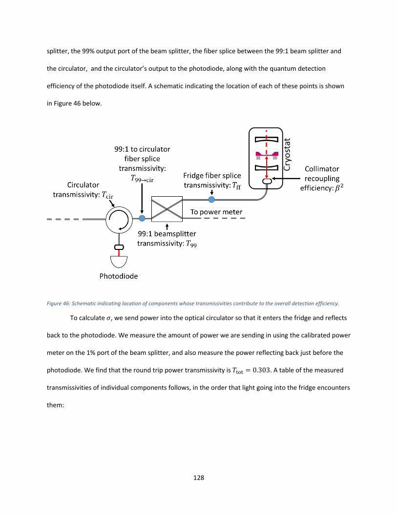
128

splitter, the 99% output port of the beam splitter, the fiber splice between the 99:1 beam splitter and

the circulator, and the circulator’s output to the photodiode, along with the quantum detection

efficiency of the photodiode itself. A schematic indicating the location of each of these points is shown

in Figure 46 below.

Figure 46: Schematic indicating location of components whose transmissivities contribute to the overall detection efficiency.

To calculate 𝜎, we send power into the optical circulator so that it enters the fridge and reflects

back to the photodiode. We measure the amount of power we are sending in using the calibrated power

meter on the 1% port of the beam splitter, and also measure the power reflecting back just before the

photodiode. We find that the round trip power transmissivity is 𝑇tot = 0.303. A table of the measured

transmissivities of individual components follows, in the order that light going into the fridge encounters

them:

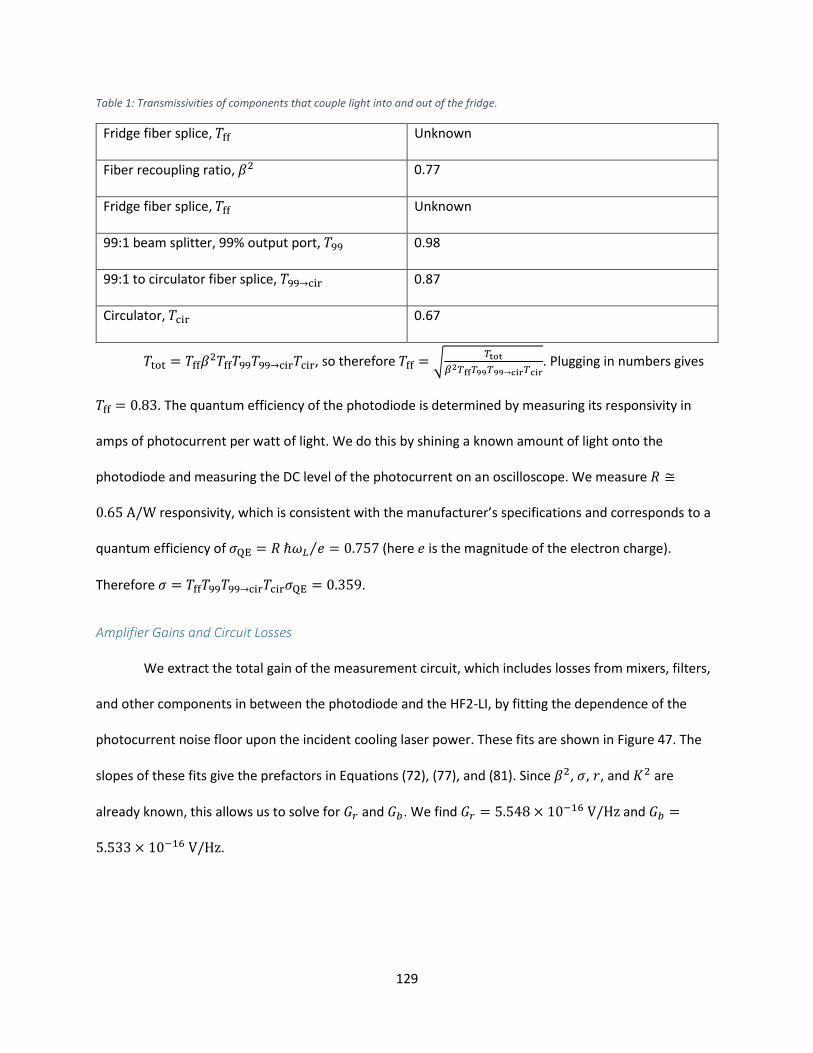
129

Table 1: Transmissivities of components that couple light into and out of the fridge.

Fridge fiber splice, 𝑇ff Unknown

Fiber recoupling ratio, 𝛽2 0.77

Fridge fiber splice, 𝑇ff Unknown

99:1 beam splitter, 99% output port, 𝑇99 0.98

99:1 to circulator fiber splice, 𝑇99→cir 0.87

Circulator, 𝑇cir 0.67

𝑇tot = 𝑇ff𝛽2𝑇ff𝑇99𝑇99→cir𝑇cir, so therefore 𝑇ff = √

𝑇tot

𝛽2𝑇ff𝑇99𝑇99→cir𝑇cir. Plugging in numbers gives

𝑇ff = 0.83. The quantum efficiency of the photodiode is determined by measuring its responsivity in

amps of photocurrent per watt of light. We do this by shining a known amount of light onto the

photodiode and measuring the DC level of the photocurrent on an oscilloscope. We measure 𝑅 ≅

0.65 A/W responsivity, which is consistent with the manufacturer’s specifications and corresponds to a

quantum efficiency of 𝜎QE = 𝑅 ℏ𝜔𝐿 𝑒⁄ = 0.757 (here 𝑒 is the magnitude of the electron charge).

Therefore 𝜎 = 𝑇ff𝑇99𝑇99→cir𝑇cir𝜎QE = 0.359.

Amplifier Gains and Circuit Losses

We extract the total gain of the measurement circuit, which includes losses from mixers, filters,

and other components in between the photodiode and the HF2-LI, by fitting the dependence of the

photocurrent noise floor upon the incident cooling laser power. These fits are shown in Figure 47. The

slopes of these fits give the prefactors in Equations (72), (77), and (81). Since 𝛽2, 𝜎, 𝑟, and 𝐾2 are

already known, this allows us to solve for 𝐺𝑟 and 𝐺𝑏. We find 𝐺𝑟 = 5.548 × 10−16 V/Hz and 𝐺𝑏 =

5.533 × 10−16 V/Hz.

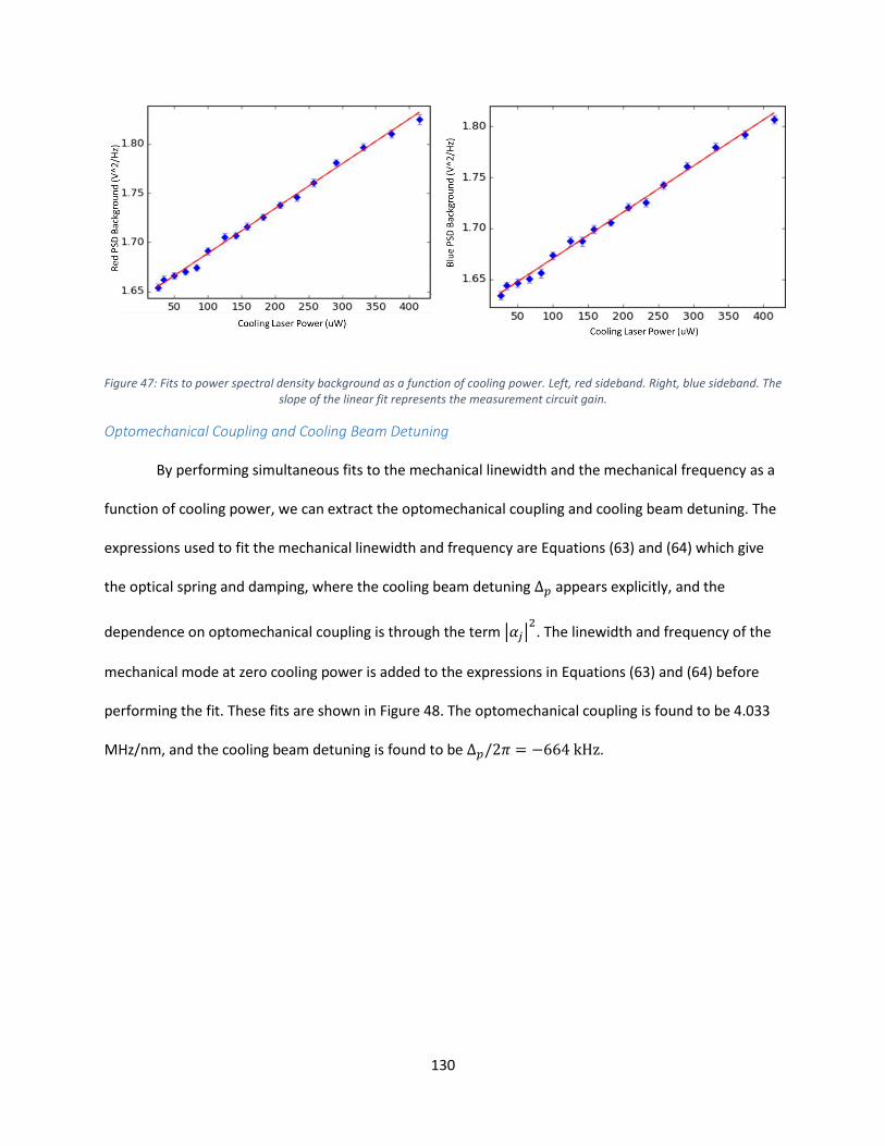
130

Figure 47: Fits to power spectral density background as a function of cooling power. Left, red sideband. Right, blue sideband. The slope of the linear fit represents the measurement circuit gain.

Optomechanical Coupling and Cooling Beam Detuning

By performing simultaneous fits to the mechanical linewidth and the mechanical frequency as a

function of cooling power, we can extract the optomechanical coupling and cooling beam detuning. The

expressions used to fit the mechanical linewidth and frequency are Equations (63) and (64) which give

the optical spring and damping, where the cooling beam detuning Δ𝑝 appears explicitly, and the

dependence on optomechanical coupling is through the term |𝛼𝑗|2

. The linewidth and frequency of the

mechanical mode at zero cooling power is added to the expressions in Equations (63) and (64) before

performing the fit. These fits are shown in Figure 48. The optomechanical coupling is found to be 4.033

MHz/nm, and the cooling beam detuning is found to be Δ𝑝/2𝜋 = −664 kHz.

131

Figure 48: Simultaneous fits to the optical damping (left) and optical spring (right) as a function of cooling power.

Bare Mechanical Linewidth

We characterize the bare linewidth of the mechanical mode using a time-domain mechanical

ringdown measurement. To perform this measurement, we use a laser that is outside of the cavity

mirrors’ high reflectivity bandwidth, a ThorLabs 1310 nm fiber laser. Use of this laser is necessary

because locking the 1064 nm laser to the cavity when the membrane is oscillating with high amplitude is

extremely difficult, and because the optical damping effect caused by 1064 nm laser perturbs the

linewidth significantly even for a weak beam that is nearly on resonance. The 1310 nm laser can enter

the cavity without any need for locking because the finesse of the cavity at 1310 nm is close to unity due

to the lower reflectivity of the mirrors at this wavelength. Also, since the finesse is so low, the

optomechanical interaction (and optical damping) is negligible.

Once the 1310 nm laser is on, we use the HF2-LI to drive the membrane at a frequency near 𝜔𝑚.

Light from the 1310 nm laser enters the cavity and reflects off of the driven membrane, carrying away

information about the membrane’s motion in the phase of the light. This light then combines with light

that promptly reflected off the cavity input mirror inside the cryostat. When the two light beams

eventually return to the optics table, they pass through a circulator which directs them to a photodiode.

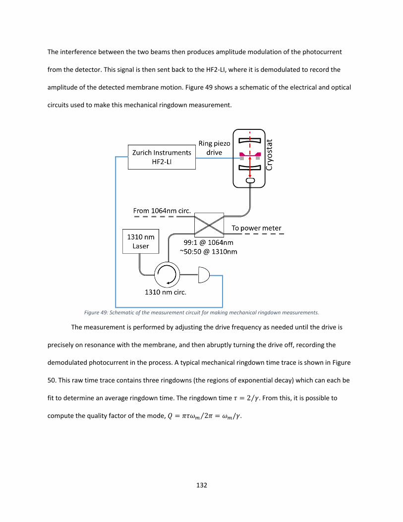
132

The interference between the two beams then produces amplitude modulation of the photocurrent

from the detector. This signal is then sent back to the HF2-LI, where it is demodulated to record the

amplitude of the detected membrane motion. Figure 49 shows a schematic of the electrical and optical

circuits used to make this mechanical ringdown measurement.

Figure 49: Schematic of the measurement circuit for making mechanical ringdown measurements.

The measurement is performed by adjusting the drive frequency as needed until the drive is

precisely on resonance with the membrane, and then abruptly turning the drive off, recording the

demodulated photocurrent in the process. A typical mechanical ringdown time trace is shown in Figure

50. This raw time trace contains three ringdowns (the regions of exponential decay) which can each be

fit to determine an average ringdown time. The ringdown time 𝜏 = 2 𝛾⁄ . From this, it is possible to

compute the quality factor of the mode, 𝑄 = 𝜋𝜏𝜔𝑚 2𝜋⁄ = 𝜔𝑚/𝛾.

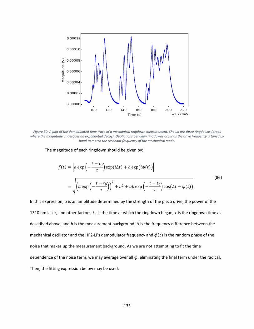
133

Figure 50: A plot of the demodulated time trace of a mechanical ringdown measurement. Shown are three ringdowns (areas where the magnitude undergoes an exponential decay). Oscillations between ringdowns occur as the drive frequency is tuned by

hand to match the resonant frequency of the mechanical mode.

The magnitude of each ringdown should be given by:

𝑓(𝑡) = |𝑎 exp (−𝑡 − 𝑡0𝜏

) exp(𝑖Δ𝑡) + 𝑏 exp(𝑖𝜙(𝑡))|

= √(𝑎 exp (−𝑡 − 𝑡0𝜏

))2

+ 𝑏2 + 𝑎𝑏 exp (−𝑡 − 𝑡0𝜏

) cos(𝛥𝑡 − 𝜙(𝑡))

(86)

In this expression, 𝑎 is an amplitude determined by the strength of the piezo drive, the power of the

1310 nm laser, and other factors, 𝑡0 is the time at which the ringdown began, 𝜏 is the ringdown time as

described above, and 𝑏 is the measurement background. Δ is the frequency difference between the

mechanical oscillator and the HF2-LI’s demodulator frequency and 𝜙(𝑡) is the random phase of the

noise that makes up the measurement background. As we are not attempting to fit the time

dependence of the noise term, we may average over all 𝜙, eliminating the final term under the radical.

Then, the fitting expression below may be used:

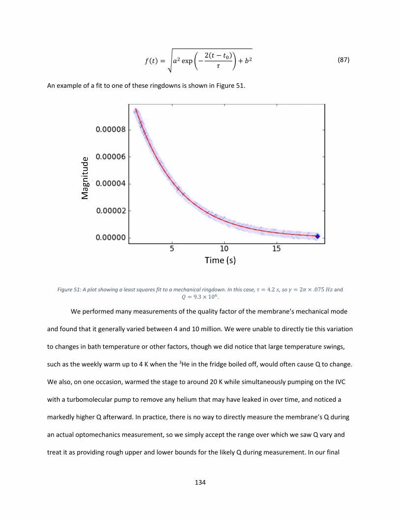
134

𝑓(𝑡) = √𝑎2 exp (−2(𝑡 − 𝑡0)

𝜏) + 𝑏2 (87)

An example of a fit to one of these ringdowns is shown in Figure 51.

Figure 51: A plot showing a least squares fit to a mechanical ringdown. In this case, 𝜏 = 4.2 𝑠, so 𝛾 = 2𝜋 × .075 𝐻𝑧 and 𝑄 = 9.3 × 106.

We performed many measurements of the quality factor of the membrane’s mechanical mode

and found that it generally varied between 4 and 10 million. We were unable to directly tie this variation

to changes in bath temperature or other factors, though we did notice that large temperature swings,

such as the weekly warm up to 4 K when the 3He in the fridge boiled off, would often cause Q to change.

We also, on one occasion, warmed the stage to around 20 K while simultaneously pumping on the IVC

with a turbomolecular pump to remove any helium that may have leaked in over time, and noticed a

markedly higher Q afterward. In practice, there is no way to directly measure the membrane’s Q during

an actual optomechanics measurement, so we simply accept the range over which we saw Q vary and

treat it as providing rough upper and lower bounds for the likely Q during measurement. In our final

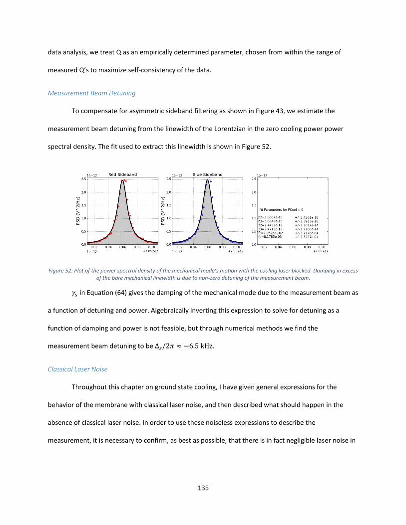
135

data analysis, we treat Q as an empirically determined parameter, chosen from within the range of

measured Q’s to maximize self-consistency of the data.

Measurement Beam Detuning

To compensate for asymmetric sideband filtering as shown in Figure 43, we estimate the

measurement beam detuning from the linewidth of the Lorentzian in the zero cooling power power

spectral density. The fit used to extract this linewidth is shown in Figure 52.

Figure 52: Plot of the power spectral density of the mechanical mode’s motion with the cooling laser blocked. Damping in excess of the bare mechanical linewidth is due to non-zero detuning of the measurement beam.

𝛾𝑠 in Equation (64) gives the damping of the mechanical mode due to the measurement beam as

a function of detuning and power. Algebraically inverting this expression to solve for detuning as a

function of damping and power is not feasible, but through numerical methods we find the

measurement beam detuning to be Δ𝑠/2𝜋 ≈ −6.5 kHz.

Classical Laser Noise

Throughout this chapter on ground state cooling, I have given general expressions for the

behavior of the membrane with classical laser noise, and then described what should happen in the

absence of classical laser noise. In order to use these noiseless expressions to describe the

measurement, it is necessary to confirm, as best as possible, that there is in fact negligible laser noise in

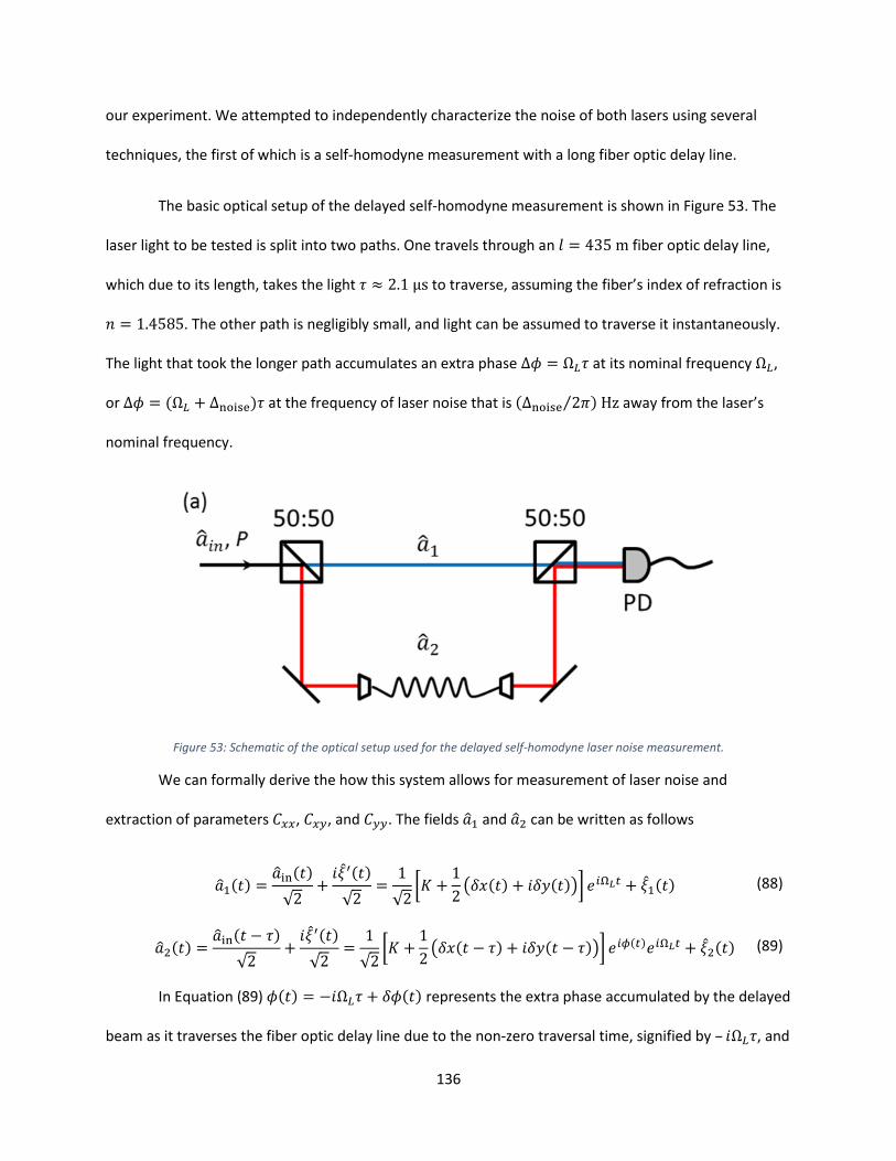
136

our experiment. We attempted to independently characterize the noise of both lasers using several

techniques, the first of which is a self-homodyne measurement with a long fiber optic delay line.

The basic optical setup of the delayed self-homodyne measurement is shown in Figure 53. The

laser light to be tested is split into two paths. One travels through an 𝑙 = 435 m fiber optic delay line,

which due to its length, takes the light 𝜏 ≈ 2.1 μs to traverse, assuming the fiber’s index of refraction is

𝑛 = 1.4585. The other path is negligibly small, and light can be assumed to traverse it instantaneously.

The light that took the longer path accumulates an extra phase Δ𝜙 = Ω𝐿𝜏 at its nominal frequency Ω𝐿,

or Δ𝜙 = (Ω𝐿 + Δnoise)𝜏 at the frequency of laser noise that is (Δnoise 2𝜋⁄ ) Hz away from the laser’s

nominal frequency.

Figure 53: Schematic of the optical setup used for the delayed self-homodyne laser noise measurement.

We can formally derive the how this system allows for measurement of laser noise and

extraction of parameters 𝐶𝑥𝑥, 𝐶𝑥𝑦, and 𝐶𝑦𝑦. The fields ��1 and ��2 can be written as follows

��1(𝑡) =��in(𝑡)

√2+𝑖𝜉′(𝑡)

√2=1

√2[𝐾 +

1

2(𝛿𝑥(𝑡) + 𝑖𝛿𝑦(𝑡))] 𝑒𝑖Ω𝐿𝑡 + 𝜉1(𝑡) (88)

��2(𝑡) =��in(𝑡 − 𝜏)

√2+𝑖𝜉′(𝑡)

√2=1

√2[𝐾 +

1

2(𝛿𝑥(𝑡 − 𝜏) + 𝑖𝛿𝑦(𝑡 − 𝜏))] 𝑒𝑖𝜙(𝑡)𝑒𝑖Ω𝐿𝑡 + 𝜉2(𝑡) (89)

In Equation (89) 𝜙(𝑡) = −𝑖Ω𝐿𝜏 + 𝛿𝜙(𝑡) represents the extra phase accumulated by the delayed

beam as it traverses the fiber optic delay line due to the non-zero traversal time, signified by – 𝑖Ω𝐿𝜏, and

137

due to large (but slow compared with 𝜏) fluctuations in the length of the delay line due to vibrational,

acoustic, or thermal effects, signified by 𝛿𝜙(𝑡). When the beams recombine at a 50:50 beam splitter,

the total optical field can be written as the sum of ��1(𝑡)/√2 and ��2(𝑡)/√2:

��(𝑡) =

1

2{[𝐾 +

1

2(𝛿𝑥(𝑡) + 𝑖(𝛿𝑦(𝑡)))] + [𝐾 +

1

2(𝛿𝑥(𝑡 − 𝜏) + 𝑖𝛿𝑦(𝑡 − 𝜏))] 𝑒𝑖𝜙(𝑡)} 𝑒𝑖Ω𝑡

+ 𝜉(𝑡)

(90)

In this expression, the total vacuum noise has been rewritten as just 𝜉(𝑡).

As in the heterodyne case, the power spectrum can be derived using the Weiner-Khinchin

theorem from the current autocorrelation function given by Equation (71), except now 𝐼(𝑡) arises from

the fields of the homodyne measurement:

𝐼(𝑡) =𝐾

2{[𝐾 +

1

2(𝛿𝑥(𝑡) + 𝛿𝑥(𝑡 − 𝜏))] (1 + cos(𝜙(𝑡))

+1

2(𝛿𝑦(𝑡) + 𝛿𝑦(𝑡 − 𝜏)) sin(𝜙(𝑡)))}

(91)

Since laser noise is generally assumed to be small, terms quadratic in 𝛿𝑥(𝑡) or 𝛿𝑦(𝑡) can be

neglected. Exploiting Equation (50) and also assuming that 𝜙 varies slowly compared to the fiber delay

such that 𝜙(𝑡 + 𝜏) ≈ 𝜙(𝑡), the first term of the current autocorrelation function can be written as

⟨: 𝐼(𝑡)𝐼(𝑡 + 𝜏): ⟩

= 𝐾2

4{4 cos4 (

𝜙(𝑡)

2)𝐾2

+ cos4 (𝜙(𝑡)

2)𝐶𝑥𝑥[2𝛿(𝑡𝑐) + 𝛿(𝑡𝑐 − 𝜏) + 𝛿(𝑡𝑐 + 𝜏)]

+ cos2 (𝜙(𝑡)

2) sin2 (

𝜙(𝑡)

2)𝐶𝑦𝑦[2𝛿(𝑡𝑐) − 𝛿(𝑡𝑐 − 𝜏) − 𝛿(𝑡𝑐 − 𝜏)]}

(92)

138

After averaging 𝜙 over the interval (0,2𝜋) to account for the fluctuations in fiber delay line

length that occur during the timescale of a measurement (measurement time 𝜏meas ≫ 𝜏), the power

spectrum is

𝑆[𝜔] = 𝐺2𝜎𝐾2

2[1 + 𝜎 (

3

4𝐶𝑥𝑥 cos

2𝜔𝜏

2+1

4𝐶𝑦𝑦 sin

2𝜔𝜏

2)] (93)

From Equation (93) it is clear that the spectrum is everywhere sensitive to shot noise,

represented by the 1 at the beginning of the expression. For classical noise, the spectrum is maximally

sensitive to amplitude noise at maxima of cos2𝜔𝜏

2, and maximally sensitive to phase noise at maxima of

sin2𝜔𝜏

2. For an approximate delay of 2.1 μs, the first phase noise sensitivity maximum occurs near 238

kHz, and the second near 713 kHz. The precise positions of these sensitivity maxima depend on the

precise delay time, which depends on the precise index of refraction of the fiber. However, due to the

short delay time of our fiber and the ensuing slow periodicity of cos2𝜔𝜏

2 and sin2

𝜔𝜏

2 the bandwidth of

the region of nearly maximum sensitivity to phase noise is many tens of kilohertz wide. Since we care

about being able to measure phase noise at 𝜔𝑚 2𝜋⁄ = 705 kHz and there is a predicted maximum less

than 10 kHz away, precisely measuring the fiber’s index of refraction and delay time is not necessary.

The coefficients of 𝐶𝑥𝑥 and 𝐶𝑦𝑦 in of Equation (93) determine the interferometer’s relative

sensitivity to each type of noise. Figure 54 shows a plot of the relative sensitivity of the delay line

interferometer to amplitude noise (blue) and phase noise (yellow) as a function of frequency after

dividing out the common coefficients 𝐺2𝜎2𝐾2 2⁄ . As can be seen in Figure 54 the interferometer is

maximally sensitive to phase noise in the region around 713 kHz.

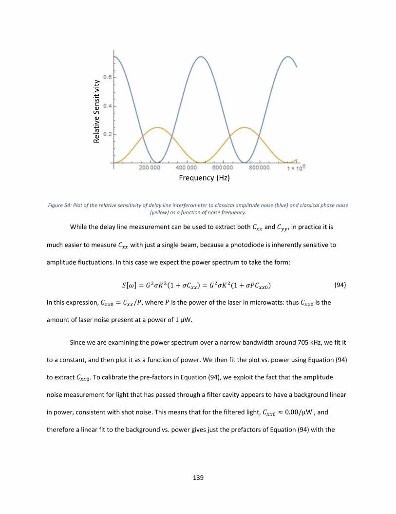
139

Figure 54: Plot of the relative sensitivity of delay line interferometer to classical amplitude noise (blue) and classical phase noise (yellow) as a function of noise frequency.

While the delay line measurement can be used to extract both 𝐶𝑥𝑥 and 𝐶𝑦𝑦, in practice it is

much easier to measure 𝐶𝑥𝑥 with just a single beam, because a photodiode is inherently sensitive to

amplitude fluctuations. In this case we expect the power spectrum to take the form:

𝑆[𝜔] = 𝐺2𝜎𝐾2(1 + 𝜎𝐶𝑥𝑥) = 𝐺2𝜎𝐾2(1 + 𝜎𝑃𝐶𝑥𝑥0) (94)

In this expression, 𝐶𝑥𝑥0 = 𝐶𝑥𝑥/𝑃, where 𝑃 is the power of the laser in microwatts: thus 𝐶𝑥𝑥0 is the

amount of laser noise present at a power of 1 μW.

Since we are examining the power spectrum over a narrow bandwidth around 705 kHz, we fit it

to a constant, and then plot it as a function of power. We then fit the plot vs. power using Equation (94)

to extract 𝐶𝑥𝑥0. To calibrate the pre-factors in Equation (94), we exploit the fact that the amplitude

noise measurement for light that has passed through a filter cavity appears to have a background linear

in power, consistent with shot noise. This means that for the filtered light, 𝐶𝑥𝑥0 ≈ 0.00/μW , and

therefore a linear fit to the background vs. power gives just the prefactors of Equation (94) with the

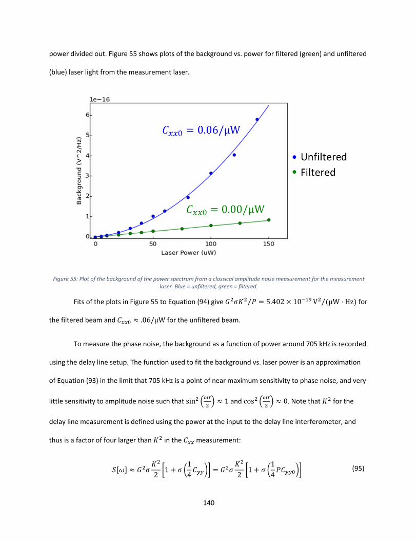
140

power divided out. Figure 55 shows plots of the background vs. power for filtered (green) and unfiltered

(blue) laser light from the measurement laser.

Figure 55: Plot of the background of the power spectrum from a classical amplitude noise measurement for the measurement laser. Blue = unfiltered, green = filtered.

Fits of the plots in Figure 55 to Equation (94) give 𝐺2𝜎𝐾2 𝑃⁄ = 5.402 × 10−19 V2 (μW ⋅ Hz)⁄ for

the filtered beam and 𝐶𝑥𝑥0 ≈ .06/μW for the unfiltered beam.

To measure the phase noise, the background as a function of power around 705 kHz is recorded

using the delay line setup. The function used to fit the background vs. laser power is an approximation

of Equation (93) in the limit that 705 kHz is a point of near maximum sensitivity to phase noise, and very

little sensitivity to amplitude noise such that sin2 (𝜔𝜏

2) ≈ 1 and cos2 (

𝜔𝜏

2) ≈ 0. Note that 𝐾2 for the

delay line measurement is defined using the power at the input to the delay line interferometer, and

thus is a factor of four larger than 𝐾2 in the 𝐶𝑥𝑥 measurement:

𝑆[𝜔] ≈ 𝐺2𝜎𝐾2

2[1 + 𝜎 (

1

4𝐶𝑦𝑦)] = 𝐺

2𝜎𝐾2

2[1 + 𝜎 (

1

4𝑃𝐶𝑦𝑦0)] (95)

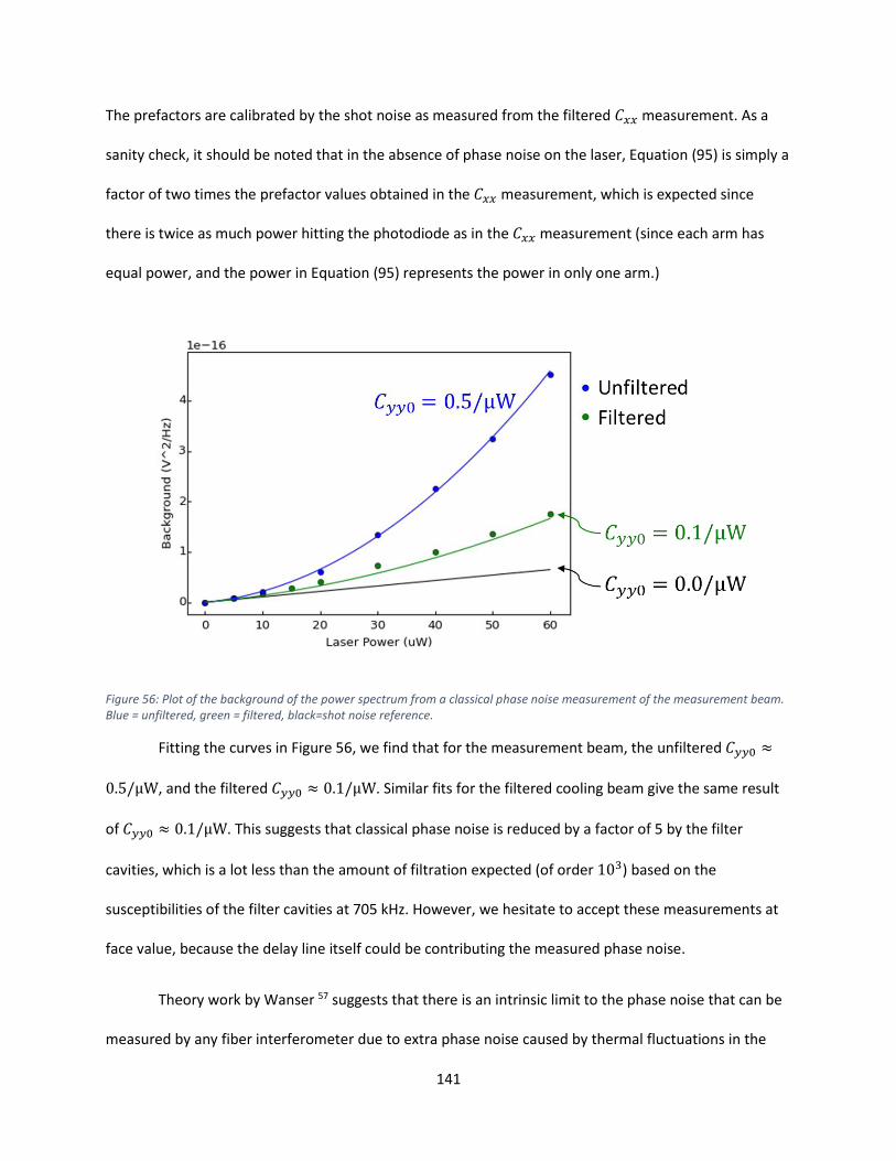
141

The prefactors are calibrated by the shot noise as measured from the filtered 𝐶𝑥𝑥 measurement. As a

sanity check, it should be noted that in the absence of phase noise on the laser, Equation (95) is simply a

factor of two times the prefactor values obtained in the 𝐶𝑥𝑥 measurement, which is expected since

there is twice as much power hitting the photodiode as in the 𝐶𝑥𝑥 measurement (since each arm has

equal power, and the power in Equation (95) represents the power in only one arm.)

Figure 56: Plot of the background of the power spectrum from a classical phase noise measurement of the measurement beam. Blue = unfiltered, green = filtered, black=shot noise reference.

Fitting the curves in Figure 56, we find that for the measurement beam, the unfiltered 𝐶𝑦𝑦0 ≈

0.5/μW, and the filtered 𝐶𝑦𝑦0 ≈ 0.1/μW. Similar fits for the filtered cooling beam give the same result

of 𝐶𝑦𝑦0 ≈ 0.1/μW. This suggests that classical phase noise is reduced by a factor of 5 by the filter

cavities, which is a lot less than the amount of filtration expected (of order 103) based on the

susceptibilities of the filter cavities at 705 kHz. However, we hesitate to accept these measurements at

face value, because the delay line itself could be contributing the measured phase noise.

Theory work by Wanser 57 suggests that there is an intrinsic limit to the phase noise that can be

measured by any fiber interferometer due to extra phase noise caused by thermal fluctuations in the

142

fiber. Since these thermal fluctuations change the effective length of the fiber, they can modulate the

phase of the light passing through the fiber, adding noise that is indistinguishable from the classical

phase noise that the fiber is being used to measure. Wanser’s expression for the spectrum of phase

noise introduced by thermal fluctuations in the fiber is

𝑆𝜙𝜙[𝑙, 𝜈] =𝜋𝑘B𝑇

2𝑙

𝜅𝜆2((𝑑𝑛

𝑑𝑇) + 𝑛𝛼𝐿)

2

ln

{

([𝑘max

2 + (2𝜋𝜈𝑐/𝑛

)2

]

2

+ (2𝜋𝜈𝐷 )

2

)

([𝑘min2 + (

2𝜋𝜈𝑐/𝑛

)2

]

2

+ (2𝜋𝜈𝐷)2

)}

(96)

In this equation, 𝑘B is Boltzmann’s constant, 𝑇 is the temperature, 𝑙 is the length of the fiber, 𝜅 is the

thermal conductivity of the fiber, 𝐷 is the thermal diffusivity of the fiber, 𝑑𝑛

𝑑𝑇 is the temperature

derivative of the fiber’s index of refraction 𝑛, 𝛼𝐿 is the linear thermal expansion coefficient of the fiber,

𝑘min = 2.405/𝑎𝑓 where 𝑎𝑓 is the fiber cladding radius, 𝑘max = 2/𝑤0 where 𝑤0 is the mode field radius,

𝑐 is the speed of light in vacuum, 𝜈 is the frequency (in Hertz) at which the spectrum is being evaluated.

After plugging reasonable estimates of these parameters into Equation (96), 𝑆𝜙𝜙[435 m,

705 kHz] ≈ 7.21 × 10−16radians2

Hz . Shot noise at one microwatt should be 𝑆𝜙𝜙

shot =ℏ𝜔𝐿

𝑃= 1.86 ×

10−13radians2

Hz. The ratio of these two should be equivalent to the expected 𝐶𝑦𝑦0 value if the additional

noise in our measurement were entirely from the intrinsic phase noise of the fiber, but it is actually

somewhat lower at 0.0039. While this suggests that our measured noise cannot be entirely attributed

to the intrinsic phase noise of the fiber, it is still an encouraging result because it gives some perspective

to the susceptibility of the fiber delay line technique to fluctuations from both internal and external

sources. Statistical fluctuations in temperature within the delay line are incredibly small, but yet theory

says that they introduce extra phase noise of magnitude equal to a few percent of shot noise even at

laser powers as low as a few microwatts.

143

Though we have no way of independently measuring the ambient acoustic noise at 705 kHz, it is

reasonable that it may have added to the statistical thermal fluctuations in the fiber at 705 kHz, perhaps

explaining the difference between the theory prediction of the intrinsic phase noise and the phase noise

we measured. Indeed, experiments which have attempted to directly measure the intrinsic noise

predicted by Wanser’s theory have taken excruciating steps to eliminate the influence of external noise

sources when performing measurements, such as using an interferometer with equal length arms co-

wound around a common spool and acoustically isolated from the environment by alternating layers of

lead and open cell foam inside a rigid aluminum box mounted on an air bladder on top of a vibrationally

isolated optical table in an empty building with air handlers turned off and a spectrum analyzer isolated

from sources of RF interference. 58 Thus we accept that we cannot obtain a reliable measurement of

𝐶𝑦𝑦0 using the delay line alone. However, we can say that since 𝐶𝑥𝑥0 is unambiguously zero, and 𝐶𝑦𝑦0 is

close to the limit of detectable phase noise using the common delay line interferometer technique, our

laser noise is likely very small.

Nonetheless, if appreciable classical laser noise is present in our setup, it should manifest in the

optomechanical experiments in several distinct ways. Noise on the measurement beam appears in the

heterodyne spectrum in three ways: (1) as an increased background, as can be seen from Equations (73)

and (78); (2) as a change in the area of the Lorentzian component of the membrane’s motion, as can be

seen from Equation (74) and Equation (79); and (3) as a non-zero anti-Lorentzian component of the

membrane’s motion, as can be seen from Equations (76) and (80). Careful inspection of the equations

reveals that the effect of laser noise on 𝐿𝑟𝑟 and 𝐿𝑏𝑏 is such that it leads to a larger asymmetry in the

sideband areas than would be the case for a noiseless laser. If this effect is not accounted for, a naive

analysis of the asymmetry between the sidebands would yield an incorrect phonon number that is too

small.

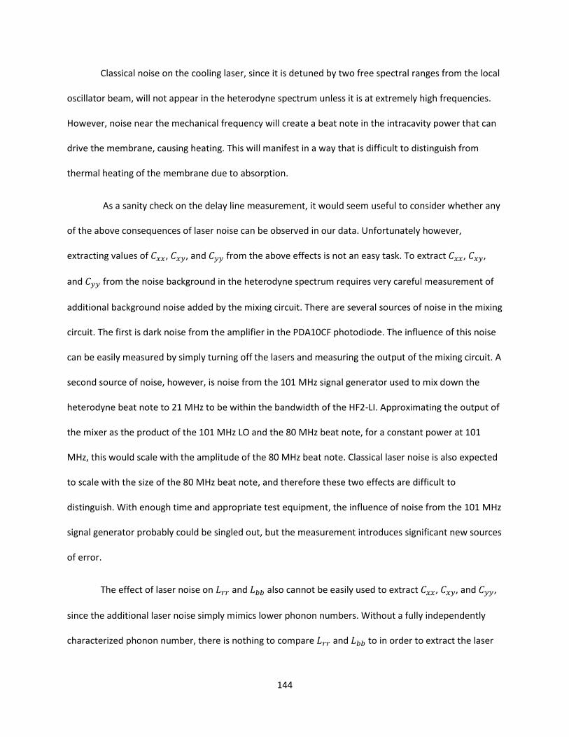
144

Classical noise on the cooling laser, since it is detuned by two free spectral ranges from the local

oscillator beam, will not appear in the heterodyne spectrum unless it is at extremely high frequencies.

However, noise near the mechanical frequency will create a beat note in the intracavity power that can

drive the membrane, causing heating. This will manifest in a way that is difficult to distinguish from

thermal heating of the membrane due to absorption.

As a sanity check on the delay line measurement, it would seem useful to consider whether any

of the above consequences of laser noise can be observed in our data. Unfortunately however,

extracting values of 𝐶𝑥𝑥, 𝐶𝑥𝑦, and 𝐶𝑦𝑦 from the above effects is not an easy task. To extract 𝐶𝑥𝑥, 𝐶𝑥𝑦,

and 𝐶𝑦𝑦 from the noise background in the heterodyne spectrum requires very careful measurement of

additional background noise added by the mixing circuit. There are several sources of noise in the mixing

circuit. The first is dark noise from the amplifier in the PDA10CF photodiode. The influence of this noise

can be easily measured by simply turning off the lasers and measuring the output of the mixing circuit. A

second source of noise, however, is noise from the 101 MHz signal generator used to mix down the

heterodyne beat note to 21 MHz to be within the bandwidth of the HF2-LI. Approximating the output of

the mixer as the product of the 101 MHz LO and the 80 MHz beat note, for a constant power at 101

MHz, this would scale with the amplitude of the 80 MHz beat note. Classical laser noise is also expected

to scale with the size of the 80 MHz beat note, and therefore these two effects are difficult to

distinguish. With enough time and appropriate test equipment, the influence of noise from the 101 MHz

signal generator probably could be singled out, but the measurement introduces significant new sources

of error.

The effect of laser noise on 𝐿𝑟𝑟 and 𝐿𝑏𝑏 also cannot be easily used to extract 𝐶𝑥𝑥, 𝐶𝑥𝑦, and 𝐶𝑦𝑦,

since the additional laser noise simply mimics lower phonon numbers. Without a fully independently

characterized phonon number, there is nothing to compare 𝐿𝑟𝑟 and 𝐿𝑏𝑏 to in order to extract the laser

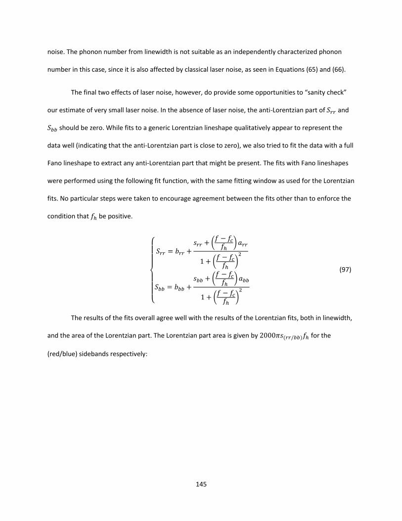
145

noise. The phonon number from linewidth is not suitable as an independently characterized phonon

number in this case, since it is also affected by classical laser noise, as seen in Equations (65) and (66).

The final two effects of laser noise, however, do provide some opportunities to “sanity check”

our estimate of very small laser noise. In the absence of laser noise, the anti-Lorentzian part of 𝑆𝑟𝑟 and

𝑆𝑏𝑏 should be zero. While fits to a generic Lorentzian lineshape qualitatively appear to represent the

data well (indicating that the anti-Lorentzian part is close to zero), we also tried to fit the data with a full

Fano lineshape to extract any anti-Lorentzian part that might be present. The fits with Fano lineshapes

were performed using the following fit function, with the same fitting window as used for the Lorentzian

fits. No particular steps were taken to encourage agreement between the fits other than to enforce the

condition that 𝑓ℎ be positive.

{

𝑆𝑟𝑟 = 𝑏𝑟𝑟 +

𝑠𝑟𝑟 + (𝑓 − 𝑓𝑐𝑓ℎ

)𝑎𝑟𝑟

1 + (𝑓 − 𝑓𝑐𝑓ℎ

)2

𝑆𝑏𝑏 = 𝑏𝑏𝑏 +𝑠𝑏𝑏 + (

𝑓 − 𝑓𝑐𝑓ℎ

) 𝑎𝑏𝑏

1 + (𝑓 − 𝑓𝑐𝑓ℎ

)2

(97)

The results of the fits overall agree well with the results of the Lorentzian fits, both in linewidth,

and the area of the Lorentzian part. The Lorentzian part area is given by 2000𝜋𝑠(𝑟𝑟/𝑏𝑏)𝑓ℎ for the

(red/blue) sidebands respectively:

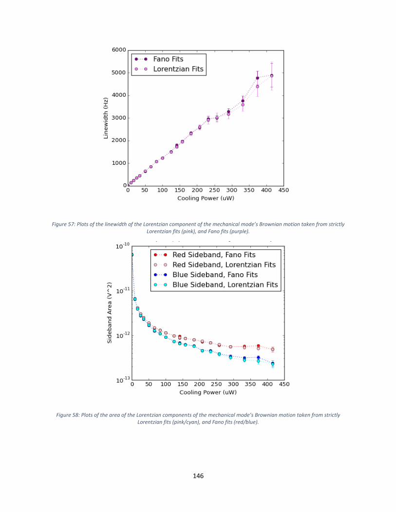
146

Figure 57: Plots of the linewidth of the Lorentzian component of the mechanical mode’s Brownian motion taken from strictly Lorentzian fits (pink), and Fano fits (purple).

Figure 58: Plots of the area of the Lorentzian components of the mechanical mode’s Brownian motion taken from strictly Lorentzian fits (pink/cyan), and Fano fits (red/blue).

147

While it is possible to characterize the Lorentzian part of the Fano fit results in terms of the area

under the Lorentzian, the anti-Lorentzian part has odd symmetry and therefore always has an area of

zero. However, it is still possible to characterize the size of the anti-Lorentzian by considering 𝐴𝑟𝑟 and

𝐴𝑏𝑏 (Equations (76) and (80)) which have units of area. In terms of the variables in the fitting

expressions (Equation (97)) these are 𝐴(𝑟𝑟/𝑏𝑏) =2𝜋×1000𝑓ℎ𝑎(𝑟𝑟/𝑏𝑏)

𝐺𝑟2𝜎𝑟𝛽2𝐾2

. For easier comparison to Figure 58

however, the gain factors need not be divided out. Thus I refer to the “area” of the anti-Lorentzian

component as the anti-Lorentzian “magnitude”, which I define as 2𝜋 × 1000𝑓ℎ𝑎(𝑟𝑟/𝑏𝑏).

Figure 59: Anti-Lorentzian component of the Fano fits as a function of cooling power for the red and the blue sidebands.

Upon first glance, the anti-Lorentzian part of the fit results shown in Figure 59 looks scattered

and does not seem to show a trend as consistent as the Lorentzian part in Figure 58. Theory predicts

that the anti-Lorentzian component should depend only on the power of the measurement/LO beams

and not depend on cooling power, so therefore the data should be flat, which they appear to be only

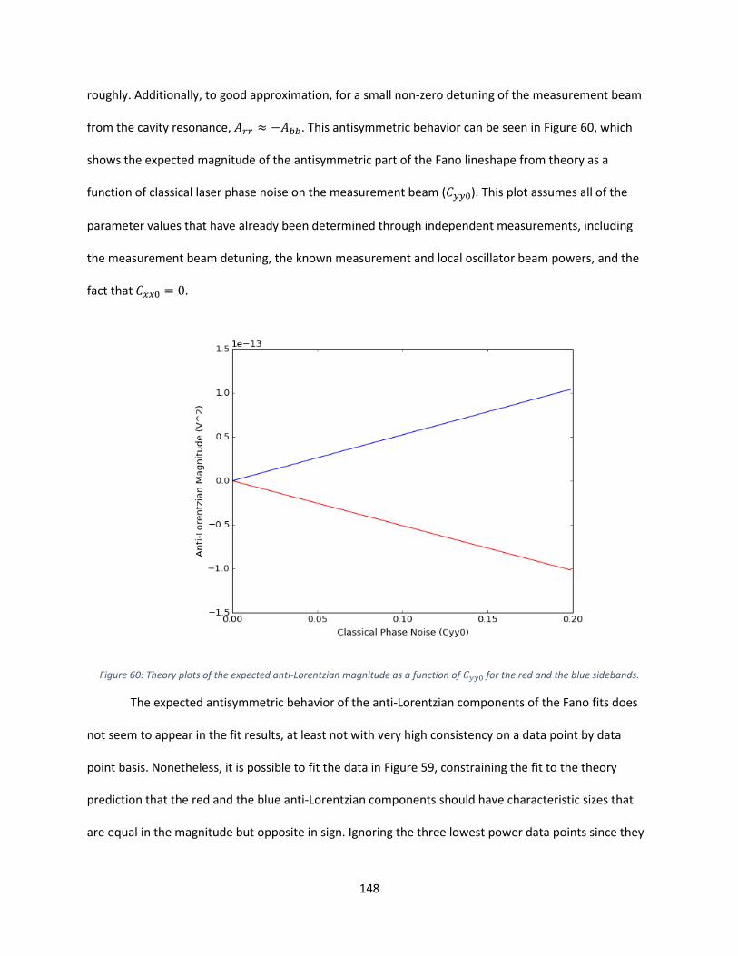
148

roughly. Additionally, to good approximation, for a small non-zero detuning of the measurement beam

from the cavity resonance, 𝐴𝑟𝑟 ≈ −𝐴𝑏𝑏. This antisymmetric behavior can be seen in Figure 60, which

shows the expected magnitude of the antisymmetric part of the Fano lineshape from theory as a

function of classical laser phase noise on the measurement beam (𝐶𝑦𝑦0). This plot assumes all of the

parameter values that have already been determined through independent measurements, including

the measurement beam detuning, the known measurement and local oscillator beam powers, and the

fact that 𝐶𝑥𝑥0 = 0.

Figure 60: Theory plots of the expected anti-Lorentzian magnitude as a function of 𝐶𝑦𝑦0 for the red and the blue sidebands.

The expected antisymmetric behavior of the anti-Lorentzian components of the Fano fits does

not seem to appear in the fit results, at least not with very high consistency on a data point by data

point basis. Nonetheless, it is possible to fit the data in Figure 59, constraining the fit to the theory

prediction that the red and the blue anti-Lorentzian components should have characteristic sizes that

are equal in the magnitude but opposite in sign. Ignoring the three lowest power data points since they

149

seem to indicate some unexpected trend, the fit results shown in Figure 61 do indicate a non-zero

average anti-Lorentzian component to the Fano fits, with characteristic size for the red and blue

sidebands of ∓(5.3 ± 0.8) × 10−14 V2 respectively. Using the defined relationship between the plotted

anti-Lorentzian magnitudes and 𝐴𝑟𝑟/𝐴𝑏𝑏 it is possible to solve for Im(��), and hence extract a value for

𝐶𝑦𝑦0 from these results.

Figure 61: Fits to the anti-Lorentzian components of the red and blue sidebands.

The value of 𝐶𝑦𝑦0 extracted from the fitted magnitudes of the anti-Lorentzian components of

the Fano fits is 𝐶𝑦𝑦0 ≈ 0.1. This value is surprisingly large, and actually agrees well with the value

obtained from the delay line measurement. However, there is still reason to question this result. First,

though the constrained fit above produces a result with reasonable uncertainty, ∓(5.3 ± 0.8) ×

10−14 V2, the red and the blue data sets independently have very large uncertainties. For example,

excluding the first three data points, the average value and standard deviation of the red data set is

(−6.7 ± 5.4) × 10−14 V2, which is an uncertainty of 81%. For the blue data set, the average value and

150

standard deviation is (3.6 ± 5.3) × 10−14 V2, which is an uncertainty of 150%, and is potentially

consistent with zero. Additionally, it is odd that fluctuations in the anti-Lorentzian magnitude

qualitatively seem to be common mode to both the red and the blue sidebands, rather than

antisymmetric about zero as expected from theory. This indicates that the change in the anti-Lorentzian

magnitudes from one cooling power to the next is probably not due to fluctuations in the amount of

noise on the measurement laser, and calls into question how well the data actually represent the laser

noise.

Ultimately, Fano lineshapes are caused by the presence of correlations between the motion of

the driven mechanical mode and the laser light used to measure that mode. The only source of such

correlations considered in our theory of heterodyne detection is classical laser noise. However, there

may be other ways in which correlations between the mechanical mode and the laser light can occur.

For example, if a different mechanical mode is present in the system, such as a mode of the membrane

chip, the cavity mirrors, or the cavity body, that mode can mechanically drive the membrane. If this

mode also couples to the laser light inside the cavity, this would introduce correlations between the

membrane’s motion and the measurement laser, resulting in a Fano lineshape.

Because our theory of heterodyne detection considers laser noise as the only source of

correlations between the measurement beam and the mechanical mode, attempting to extract a value

of 𝐶𝑦𝑦0 from a Fano lineshape whose source is not classical laser noise will give an incorrect result.

While it is true that the coupling between this hypothetical extra mode and the measurement beam

means that there is extra “noise” on the laser as far as the membrane is concerned, the heterodyne

detection theory models noise with particular properties: (1) the noise is white within a bandwidth ≫ ��

around 𝜔𝑚, (2) the noise on the measurement beam is not correlated with the noise on the cooling

beam, and (3) the coupling between the noise and the mechanical motion is entirely described by the

151

cavity enhanced optomechanical coupling 𝛼𝑗. Noise from an additional mechanical mode need not

satisfy any of these properties and thus cannot be described by this model. Such noise could, for

example, strongly drive the membrane mode mechanically but only weakly couple to the laser. This

could result in a large anti-Lorentizian component in the Fano fits, but would not necessarily introduce

much additional classical noise on the lasers – which is an important characteristic, since as will be

discussed below, there is strong evidence that the noise on at least the cooling beam was very close to

zero.

Whether or not this speculation about the causes of the Fano lineshapes holds any merit, there

is compelling evidence that the laser noise on at least the cooling beam was close to zero. In the

heterodyne detection theory, classical laser noise ultimately has two effects:

1. The equations for 𝐿𝑟𝑟 and 𝐿𝑏𝑏 indicate that the sideband asymmetry will be affected by

the presence of laser noise on the measurement beam, making the sideband ratio

larger.

2. The equation for 𝑛𝑚 (Equation (65)) indicates that 𝑛𝑚 itself is also affected by classical

laser noise on both lasers, with excess laser noise causing 𝑛𝑚 to become larger. Since

𝜉 → 1 for large 𝑛𝑚, this makes the sideband ratio smaller.

Theory plots of the sideband asymmetry as a function of cooling laser power which account for

these two effects with the amount of laser noise on the measurement and the cooling lasers suggested

by the delay line and Fano fit techniques do not agree well with the experimentally measured sideband

asymmetry. The solid green line in Figure 62 shows the expected sideband asymmetry for noiseless

lasers. The dashed line shows the expected sideband asymmetry if the measurement laser has 𝐶𝑦𝑦0 =

0.1. Admittedly, this is a small enough change in the expected sideband asymmetry that qualitatively,

the data still agrees with the theory line. However, the dashed lime line in Figure 62 shows the expected

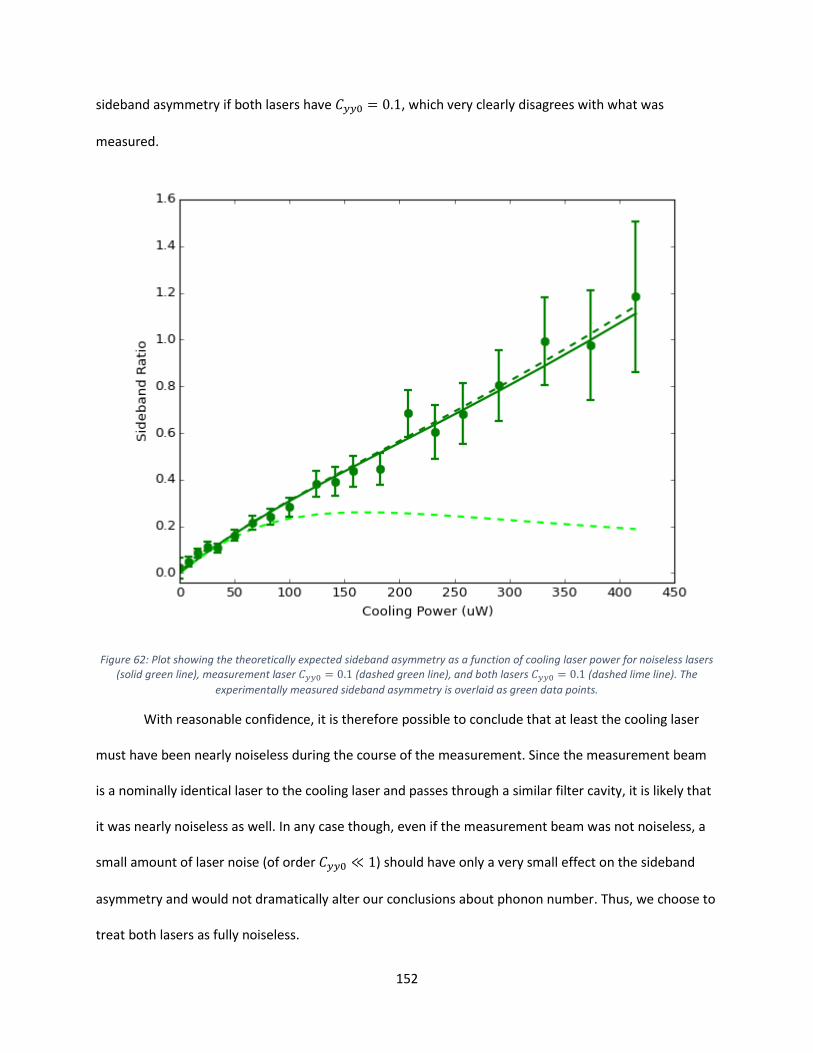
152

sideband asymmetry if both lasers have 𝐶𝑦𝑦0 = 0.1, which very clearly disagrees with what was

measured.

Figure 62: Plot showing the theoretically expected sideband asymmetry as a function of cooling laser power for noiseless lasers (solid green line), measurement laser 𝐶𝑦𝑦0 = 0.1 (dashed green line), and both lasers 𝐶𝑦𝑦0 = 0.1 (dashed lime line). The

experimentally measured sideband asymmetry is overlaid as green data points.

With reasonable confidence, it is therefore possible to conclude that at least the cooling laser

must have been nearly noiseless during the course of the measurement. Since the measurement beam

is a nominally identical laser to the cooling laser and passes through a similar filter cavity, it is likely that

it was nearly noiseless as well. In any case though, even if the measurement beam was not noiseless, a

small amount of laser noise (of order 𝐶𝑦𝑦0 ≪ 1) should have only a very small effect on the sideband

asymmetry and would not dramatically alter our conclusions about phonon number. Thus, we choose to

treat both lasers as fully noiseless.

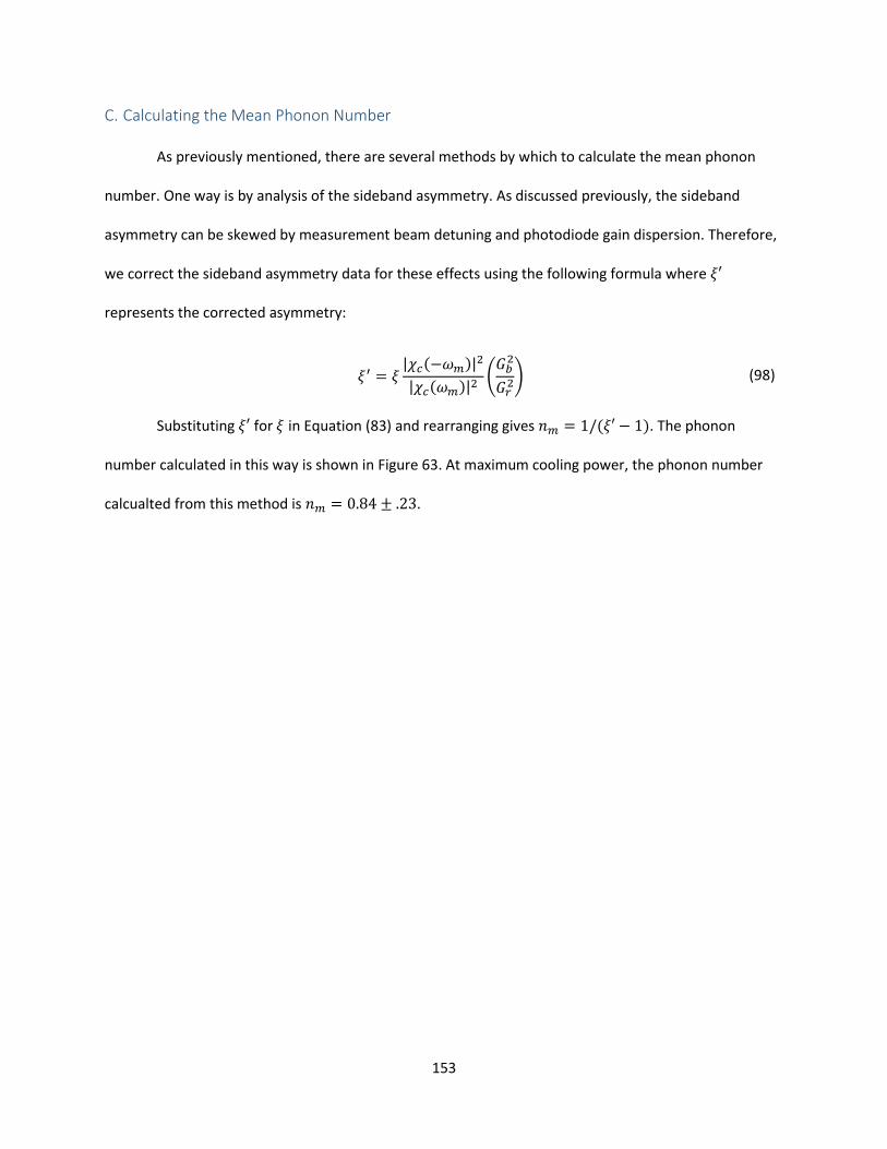
153

C. Calculating the Mean Phonon Number

As previously mentioned, there are several methods by which to calculate the mean phonon

number. One way is by analysis of the sideband asymmetry. As discussed previously, the sideband

asymmetry can be skewed by measurement beam detuning and photodiode gain dispersion. Therefore,

we correct the sideband asymmetry data for these effects using the following formula where 𝜉′

represents the corrected asymmetry:

𝜉′ = 𝜉|𝜒𝑐(−𝜔𝑚)|

2

|𝜒𝑐(𝜔𝑚)|2 (

𝐺𝑏2

𝐺𝑟2) (98)

Substituting 𝜉′ for 𝜉 in Equation (83) and rearranging gives 𝑛𝑚 = 1/(𝜉′ − 1). The phonon

number calculated in this way is shown in Figure 63. At maximum cooling power, the phonon number

calcualted from this method is 𝑛𝑚 = 0.84 ± .23.

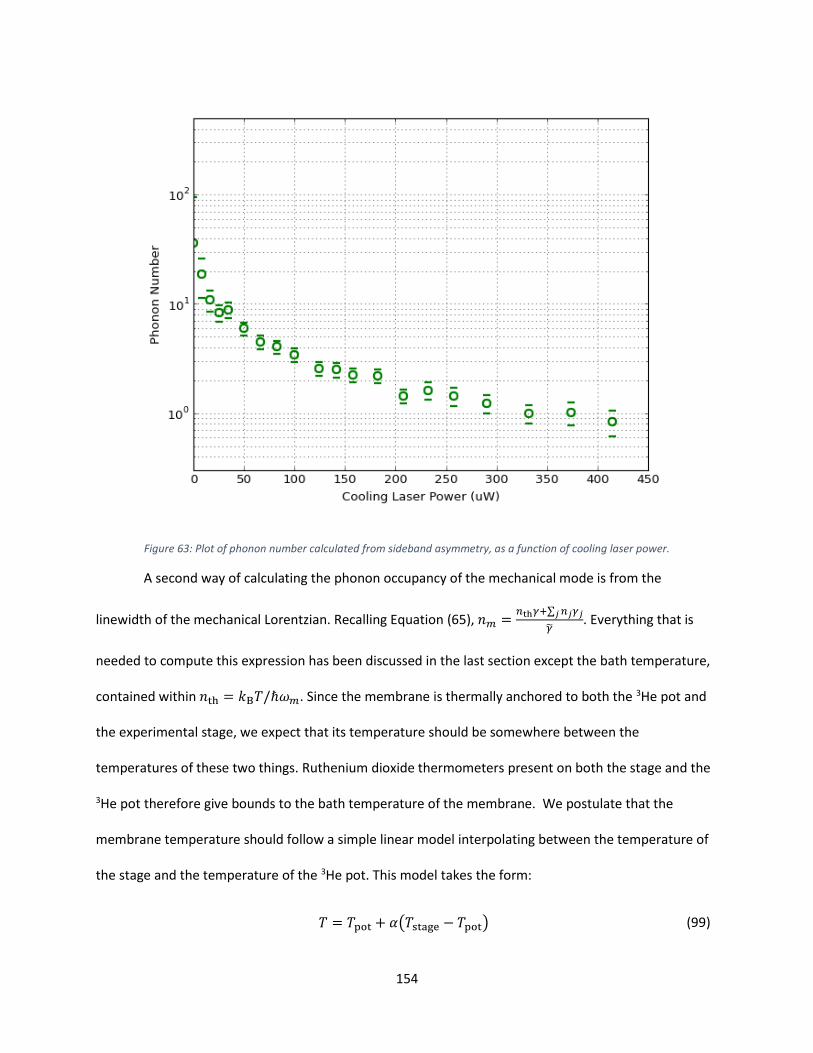
154

Figure 63: Plot of phonon number calculated from sideband asymmetry, as a function of cooling laser power.

A second way of calculating the phonon occupancy of the mechanical mode is from the

linewidth of the mechanical Lorentzian. Recalling Equation (65), 𝑛𝑚 =𝑛th𝛾+∑ 𝑛𝑗𝛾𝑗𝑗

��. Everything that is

needed to compute this expression has been discussed in the last section except the bath temperature,

contained within 𝑛th = 𝑘B𝑇/ℏ𝜔𝑚. Since the membrane is thermally anchored to both the 3He pot and

the experimental stage, we expect that its temperature should be somewhere between the

temperatures of these two things. Ruthenium dioxide thermometers present on both the stage and the

3He pot therefore give bounds to the bath temperature of the membrane. We postulate that the

membrane temperature should follow a simple linear model interpolating between the temperature of

the stage and the temperature of the 3He pot. This model takes the form:

𝑇 = 𝑇pot + 𝛼(𝑇stage − 𝑇pot) (99)

155

The value of 𝛼 is unknown a priori. We determine 𝛼 using a technique based on least squares

optimization. The procedure used involves minimization of an error function which characterizes the

difference between the phonon number calculated from sideband asymmetry and the phonon number

from linewidth. The form of the error function is as follows:

𝜖(𝛼) = ∑(1

𝑛𝑚(𝛾)−

1

𝑛𝑚(𝜉′))

2

(100)

In this expression, 𝑛𝑚(𝛾)

is the phonon number from the linewidth, and 𝑛𝑚(𝜉′)

is the phonon number from

sideband asymmetry. The summation is over all cooling powers at which data was collected during the

measurement. The reason for using the difference between the inverse phonon numbers rather than

the difference between the phonon numbers themselves is to minimize the impact that low cooling

power (large phonon number) data points have on the error function. Since the ratio of the sidebands

quickly approaches unity when 𝑛𝑚 > 1, sideband asymmetry is a particularly poor metric for computing

phonon number at low cooling powers. Therefore we seek to limit the influence that these low cooling

power/high phonon number data points have in the least squares optimization.

Before performing the optimization technique, we need to select a membrane quality factor

from within the range measured by the mechanical ringdown technique. Since 𝛾 ∝ 1/𝑄 and 𝑇 appear as

a product in the equation for phonon number as a function of linewidth, they are not fully independent

of each other. However, due to the constraints placed on 𝑇 by the linear model used (Equation (99)), the

optimization technique is not able to fully compensate for multiplicative errors in 𝑄 just by varying 𝑇.

Therefore, we empirically selected a value of 𝑄 = 4.5 × 106, which is within the range of variability

measured using the mechanical ringdown technique, as this value together with the optimization

technique to find 𝛼 seemed to best reproduce the sideband asymmetry phonon number data.

156

One could argue that the empirically determined choice of 𝑄 is in essence a poor manual least

squares optimization and that it would be sensible to simply do a multivariable least squares

optimization on 𝑄 and 𝛼. However, attempts to do this showed that the global minimum of the error

function occurs when 𝑄 ≈ 2 × 106 and 𝛼 ≈ 0. This would imply that the membrane quality factor was

smaller during the cooling measurement than it ever was during many different independent

measurements by the ringdown technique, and also that the membrane was completely unaffected by

the temperatures of the 3He pot and the stage. These two implications are inconsistent with prior

knowledge and physically unreasonable. Therefore, we decided to stick with our empirically determined

𝑄 = 4.5 × 106 and optimize just on 𝛼.

In any case, upon minimizing the error function between the phonon numbers with 𝑄 = 4.5 ×

106, we find that 𝛼 = 0.498. The inferred bath temperature as a function of cooling power with this

value of 𝛼 is plotted in Figure 64.

Figure 64: Plot of the membrane temperature computed using the linear model described in the text with 𝛼 = .498 (solid blue dots). The 3He pot temperature is shown by the hollow dots on the bottom, and the stage temperature by the hollow dots on the

top.

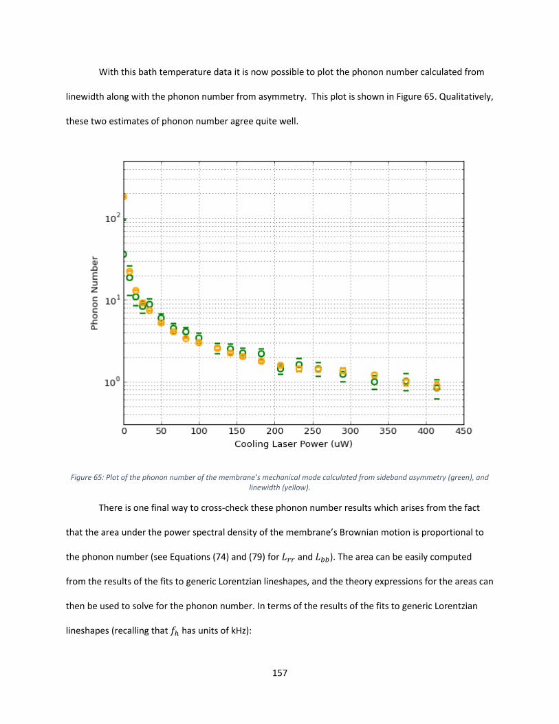
157

With this bath temperature data it is now possible to plot the phonon number calculated from

linewidth along with the phonon number from asymmetry. This plot is shown in Figure 65. Qualitatively,

these two estimates of phonon number agree quite well.

Figure 65: Plot of the phonon number of the membrane’s mechanical mode calculated from sideband asymmetry (green), and linewidth (yellow).

There is one final way to cross-check these phonon number results which arises from the fact

that the area under the power spectral density of the membrane’s Brownian motion is proportional to

the phonon number (see Equations (74) and (79) for 𝐿𝑟𝑟 and 𝐿𝑏𝑏). The area can be easily computed

from the results of the fits to generic Lorentzian lineshapes, and the theory expressions for the areas can

then be used to solve for the phonon number. In terms of the results of the fits to generic Lorentzian

lineshapes (recalling that 𝑓ℎ has units of kHz):

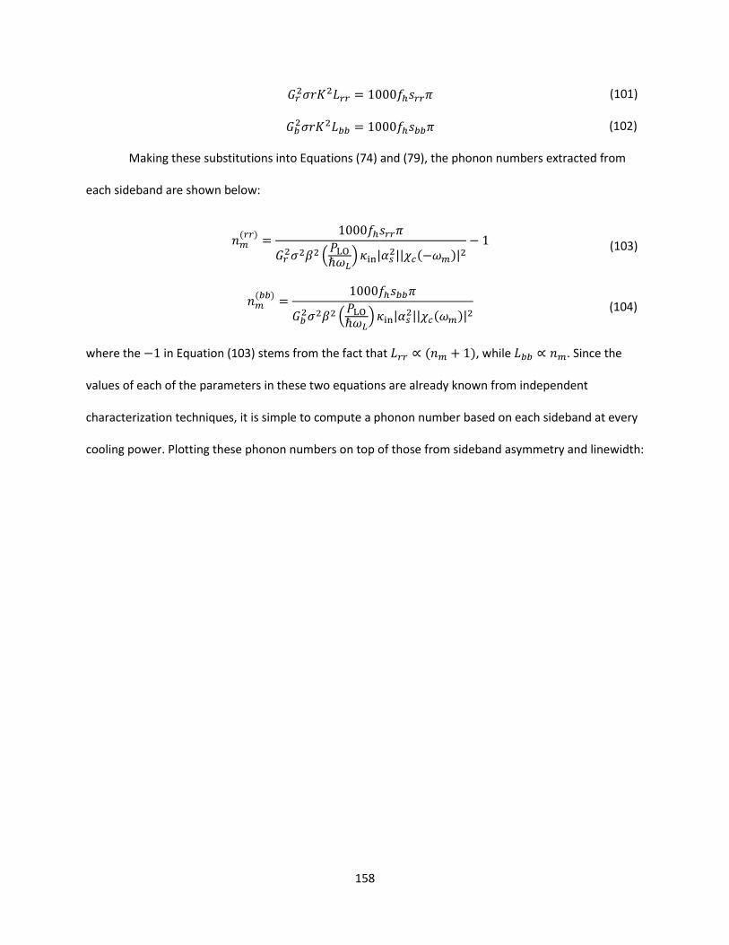
158

𝐺𝑟2𝜎𝑟𝐾2𝐿𝑟𝑟 = 1000𝑓ℎ𝑠𝑟𝑟𝜋 (101)

𝐺𝑏2𝜎𝑟𝐾2𝐿𝑏𝑏 = 1000𝑓ℎ𝑠𝑏𝑏𝜋 (102)

Making these substitutions into Equations (74) and (79), the phonon numbers extracted from

each sideband are shown below:

𝑛𝑚(𝑟𝑟)

=1000𝑓ℎ𝑠𝑟𝑟𝜋

𝐺𝑟2𝜎2𝛽2 (

𝑃LOℏ𝜔𝐿

)𝜅in|𝛼𝑠2||𝜒𝑐(−𝜔𝑚)|

2− 1 (103)

𝑛𝑚(𝑏𝑏)

=1000𝑓ℎ𝑠𝑏𝑏𝜋

𝐺𝑏2𝜎2𝛽2 (

𝑃LOℏ𝜔𝐿

)𝜅in|𝛼𝑠2||𝜒𝑐(𝜔𝑚)|

2 (104)

where the −1 in Equation (103) stems from the fact that 𝐿𝑟𝑟 ∝ (𝑛𝑚 + 1), while 𝐿𝑏𝑏 ∝ 𝑛𝑚. Since the

values of each of the parameters in these two equations are already known from independent

characterization techniques, it is simple to compute a phonon number based on each sideband at every

cooling power. Plotting these phonon numbers on top of those from sideband asymmetry and linewidth:

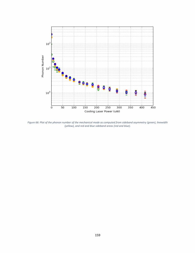
159

Figure 66: Plot of the phonon number of the mechanical mode as computed from sideband asymmetry (green), linewidth (yellow), and red and blue sideband areas (red and blue).

160

Lastly, since all of the parameters of the theory have been characterized, it is possible to directly

compute the phonon number expected for each cooling power to compare with the data. This theory

prediction is shown on top of the data in Figure 67.

Figure 67: Final plot of the phonon number of the mechanical mode calculated by four techniques, along with a comparison to the theory prediction (black line).

The theory line, as expected, agrees best with the linewidth- and area-extracted phonon

numbers at low cooling powers, confirming that sideband asymmetry is a poor estimate of phonon

number when the sideband ratio is close to unity. Overall, the data agree quite well with each other as

well as with the theory line at higher cooling powers. Since the data points in the plot are generally

larger than the difference between them, it is useful to also look at a plot of the inverse phonon

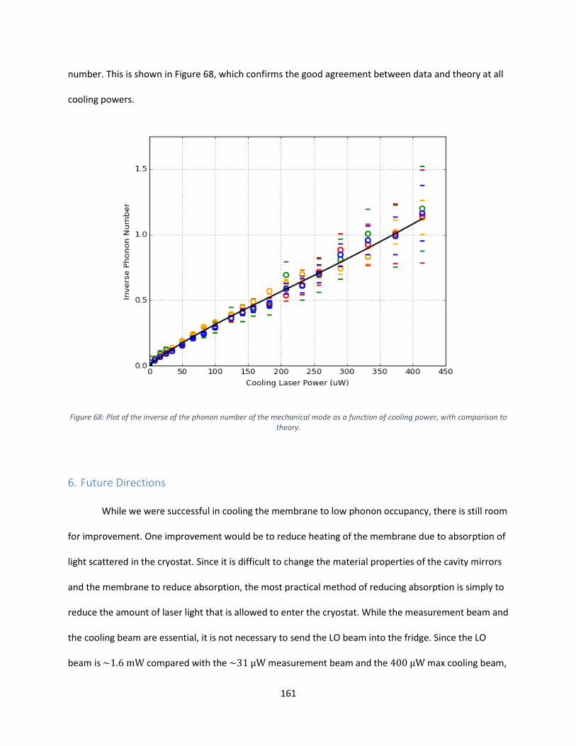
161

number. This is shown in Figure 68, which confirms the good agreement between data and theory at all

cooling powers.

Figure 68: Plot of the inverse of the phonon number of the mechanical mode as a function of cooling power, with comparison to theory.

6. Future Directions

While we were successful in cooling the membrane to low phonon occupancy, there is still room

for improvement. One improvement would be to reduce heating of the membrane due to absorption of

light scattered in the cryostat. Since it is difficult to change the material properties of the cavity mirrors

and the membrane to reduce absorption, the most practical method of reducing absorption is simply to

reduce the amount of laser light that is allowed to enter the cryostat. While the measurement beam and

the cooling beam are essential, it is not necessary to send the LO beam into the fridge. Since the LO

beam is ~1.6 mW compared with the ~31 μW measurement beam and the 400 μW max cooling beam,

162

keeping the LO beam out of the fridge could result in decreased absorptive heating by a factor of a

several. It is true that the large intracavity power from the measurement beam dwarfs the LO beam, but

practice has shown that the LO beam is the dominant contributor to changes in the thermal bath

temperature as indicated by the stage and 3He pot thermometers. Since the LO beam does not enter the

cavity, heating of the membrane due to the LO beam likely occurs indirectly through the membrane’s

thermal heatsinking wires to the 3He pot and through its mechanical connections with the stage.

A membrane mode with higher quality factor would also aid in getting to lower phonon

numbers. The optical damping produced by the cooling beam should be unchanged by membrane Q, but

the cooling factor ~𝛾𝑝/𝛾 will become larger if the starting linewidth is smaller. Other groups have

reported measuring incredibly high quality factors (𝑄 > 1 × 108) in similar membranes cooled below 20

mK in a dilution refrigerator. 59 While the effects of optical absorption may prevent maintaining a

temperature this low, it is nonetheless worth investigating whether a higher Q might be possible by

further cryogenic cooling of the membrane.

The Regal group has studied the effect of patterning the membrane chip to form a phononic

crystal around the membrane. 60 The acoustic band gap created by the phononic crystal provides

isolation between membrane’s mechanical modes and the environment. Though early results have not

shown significant increases the mechanical quality factors of membrane modes due to the phononic

crystal, future refinements to the phononic crystal’s fabrication techniques may yield improvements.

Additionally, the mechanical properties of membranes suspended within these phononic crystals have

not been studied at cryogenic temperatures.

As I mentioned in the introduction, while an accomplishment in itself, ground state cooling is

actually just a step along the road to future experiments and applications in quantum computing.

Preparation of Fock or arbitrary quantum states, and the use of mechanical oscillators as quantum

163

memory elements both benefit from oscillators that have been cooled to reduce the influence of the

thermal bath, as do proposed experiments to directly observe quantization of the mechanical

oscillator’s energy levels. Proposals for the latter of these, in fact, benefit both from ground state

cooling, and the ability to couple the optical mode quadratically to the position of the membrane. In the

second half of this dissertation, I will present our results studying the classical dynamics of our system

with this type of quadratic coupling.

164

IV. Quadratic Optomechanics

The physics underlying the ground state cooling experiment just described was based on a

Hamiltonian in which the resonant frequency of a single cavity mode scaled linearly with the

displacement of the mechanical oscillator. As described briefly in the section General Treatment of a

Membrane in a Cavity by Perturbation Theory, there are places within the cavity spectrum of a

membrane-in-the-middle system where this description of the relationship between the cavity

eigenmodes and the membrane’s position is not correct. The presence of the membrane within the

cavity induces coupling between optical modes that would normally be orthogonal, and this coupling is

strongly affected by the position, tip, and tilt of the membrane. In regions where normally orthogonal

cavity modes cross, coupling between the modes due to the membrane can cause the modes to avoid

each other. 37, 43, 49 At these avoided crossings, the perturbed optical modes can exhibit a frequency

dependence which scales quadratically with membrane position rather than linearly. This quadratic

coupling is predicted to be useful for producing squeezed optical and mechanical states 61 and for

studying the phonon statistics of a driven mechanical oscillator. 62, 63

There have been many theoretical and experimental studies of the static spectroscopy of

avoided crossings in various optomechanical systems. 37, 43, 49, 64, 65, 66, 67, 68 Fewer experiments have

studied the dynamical effects that arise from the non-linear coupling between the cavity mode and

mechanical oscillator. 66, 67, 68 In this chapter I will present a theoretical description of, as well as an

experimental study of, the dynamics arising from avoided crossings between cavity modes in a

membrane-in-the-middle system. In particular, I will present results systematically characterizing the

optical spring and optical damping in the vicinity of an avoided crossing, including their dependence on

membrane position, laser detuning, and laser power. Using these results I will both show and explain

the differences between linear and quadratic optomechanical coupling. Finally, I will present a

165

measurement exploiting quadratic optomechanical coupling to perform a measurement of classical

fluctuations of the intracavity photon number, a first step toward using quadratic coupling to detect

non-classical fluctuations in a driven oscillator. 62, 63

1. Introduction to Avoided Crossings

Using the theory described in the section General Treatment of a Membrane in a Cavity by

Perturbation Theory, the effect of the membrane’s position, tip, and tilt on the optical modes of the

cavity can be predicted. As the perturbation theory integrals are easiest to compute numerically, I will

use parameters appropriate for the membrane-in-the-middle system used in this experiment. Namely,

these are: membrane thickness 𝐿𝑑 = 50 nm, cavity length 𝐿 = 3.7 cm, cavity mirror radii of curvature

𝑅 = 5 cm, membrane index of refraction 𝑛SiN = 2.0, and laser wavelength 𝜆 = 1064 nm. We can start

by considering the TEM0,0 singlet mode, and the TEM2,0, TEM1,1 and TEM0,2 triplet modes. For a

membrane located very close to the cavity waist with no tip or tilt relative to the cavity’s optical axis, the

three triplet modes are completely degenerate by symmetry and exhibit periodic crossings with the

singlet mode of the next longitudinal mode number. This is shown in Figure 69 below, where the

degenerate triplet modes are the lower of the two sinusoidal curves.

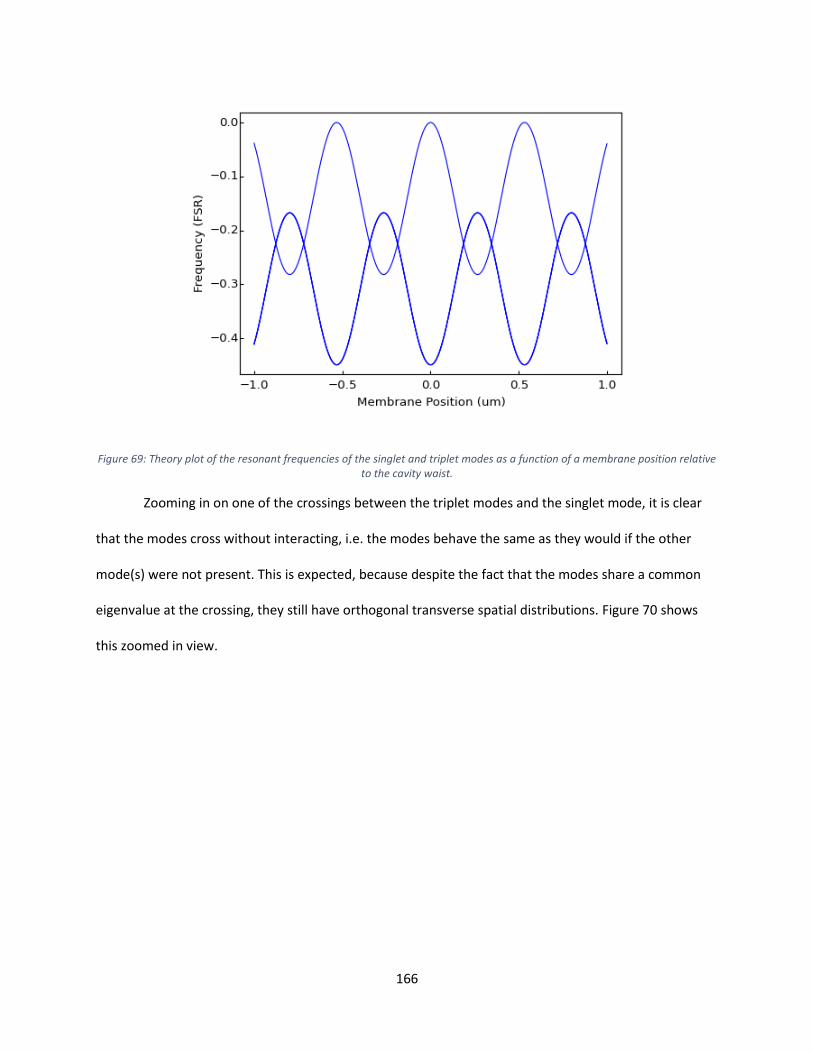
166

Figure 69: Theory plot of the resonant frequencies of the singlet and triplet modes as a function of a membrane position relative to the cavity waist.

Zooming in on one of the crossings between the triplet modes and the singlet mode, it is clear

that the modes cross without interacting, i.e. the modes behave the same as they would if the other

mode(s) were not present. This is expected, because despite the fact that the modes share a common

eigenvalue at the crossing, they still have orthogonal transverse spatial distributions. Figure 70 shows

this zoomed in view.

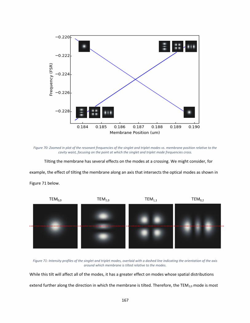
167

Figure 70: Zoomed in plot of the resonant frequencies of the singlet and triplet modes vs. membrane position relative to the cavity waist, focusing on the point at which the singlet and triplet mode frequencies cross.

Tilting the membrane has several effects on the modes at a crossing. We might consider, for

example, the effect of tilting the membrane along an axis that intersects the optical modes as shown in

Figure 71 below.

Figure 71: Intensity profiles of the singlet and triplet modes, overlaid with a dashed line indicating the orientation of the axis around which membrane is tilted relative to the modes.

While this tilt will affect all of the modes, it has a greater effect on modes whose spatial distributions

extend further along the direction in which the membrane is tilted. Therefore, the TEM2,0 mode is most

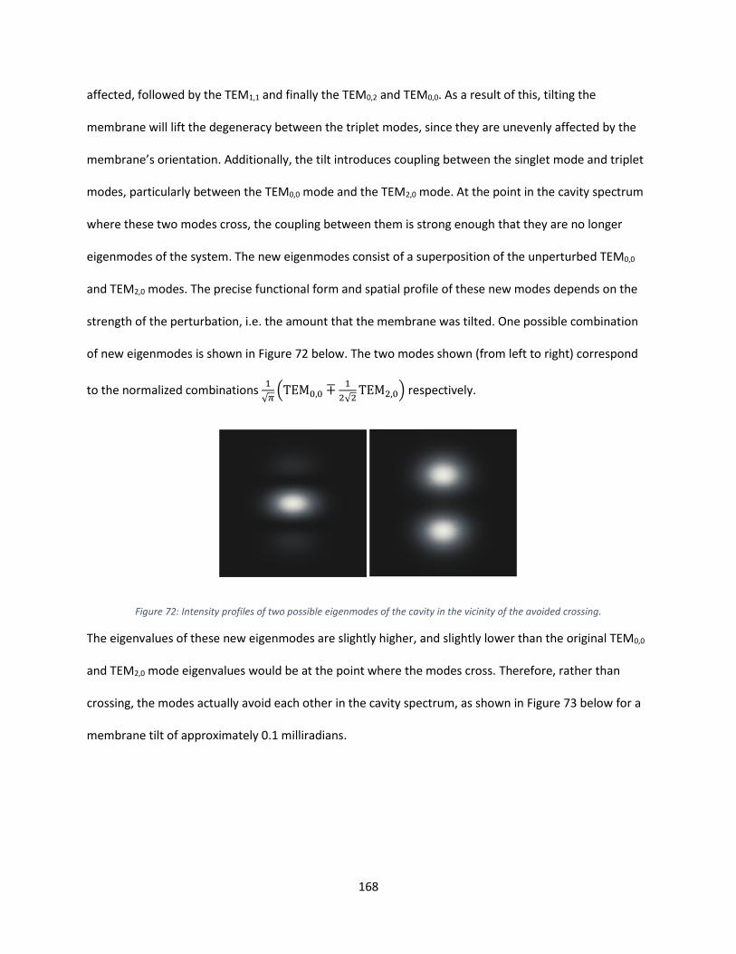
168

affected, followed by the TEM1,1 and finally the TEM0,2 and TEM0,0. As a result of this, tilting the

membrane will lift the degeneracy between the triplet modes, since they are unevenly affected by the

membrane’s orientation. Additionally, the tilt introduces coupling between the singlet mode and triplet

modes, particularly between the TEM0,0 mode and the TEM2,0 mode. At the point in the cavity spectrum

where these two modes cross, the coupling between them is strong enough that they are no longer

eigenmodes of the system. The new eigenmodes consist of a superposition of the unperturbed TEM0,0

and TEM2,0 modes. The precise functional form and spatial profile of these new modes depends on the

strength of the perturbation, i.e. the amount that the membrane was tilted. One possible combination

of new eigenmodes is shown in Figure 72 below. The two modes shown (from left to right) correspond

to the normalized combinations 1

√𝜋(TEM0,0 ∓

1

2√2TEM2,0) respectively.

Figure 72: Intensity profiles of two possible eigenmodes of the cavity in the vicinity of the avoided crossing.

The eigenvalues of these new eigenmodes are slightly higher, and slightly lower than the original TEM0,0

and TEM2,0 mode eigenvalues would be at the point where the modes cross. Therefore, rather than

crossing, the modes actually avoid each other in the cavity spectrum, as shown in Figure 73 below for a

membrane tilt of approximately 0.1 milliradians.

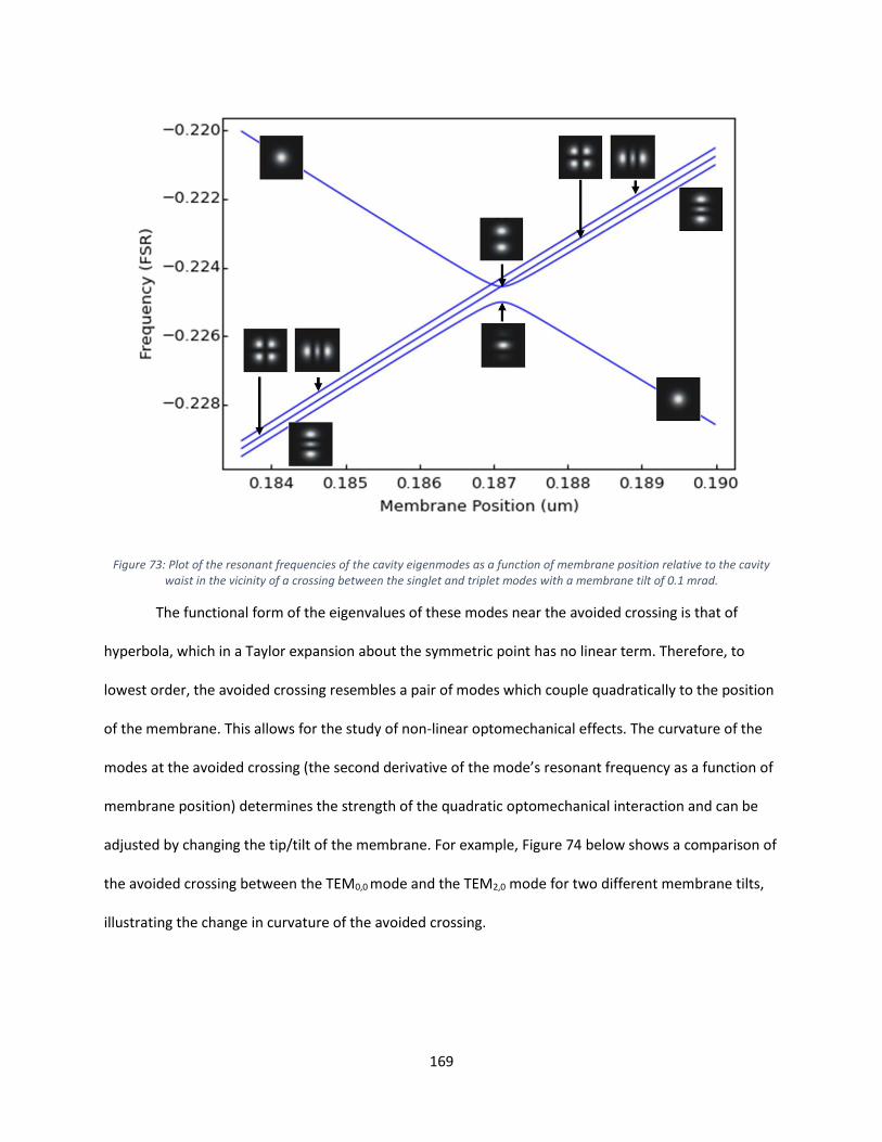
169

Figure 73: Plot of the resonant frequencies of the cavity eigenmodes as a function of membrane position relative to the cavity waist in the vicinity of a crossing between the singlet and triplet modes with a membrane tilt of 0.1 mrad.

The functional form of the eigenvalues of these modes near the avoided crossing is that of

hyperbola, which in a Taylor expansion about the symmetric point has no linear term. Therefore, to

lowest order, the avoided crossing resembles a pair of modes which couple quadratically to the position

of the membrane. This allows for the study of non-linear optomechanical effects. The curvature of the

modes at the avoided crossing (the second derivative of the mode’s resonant frequency as a function of

membrane position) determines the strength of the quadratic optomechanical interaction and can be

adjusted by changing the tip/tilt of the membrane. For example, Figure 74 below shows a comparison of

the avoided crossing between the TEM0,0 mode and the TEM2,0 mode for two different membrane tilts,

illustrating the change in curvature of the avoided crossing.

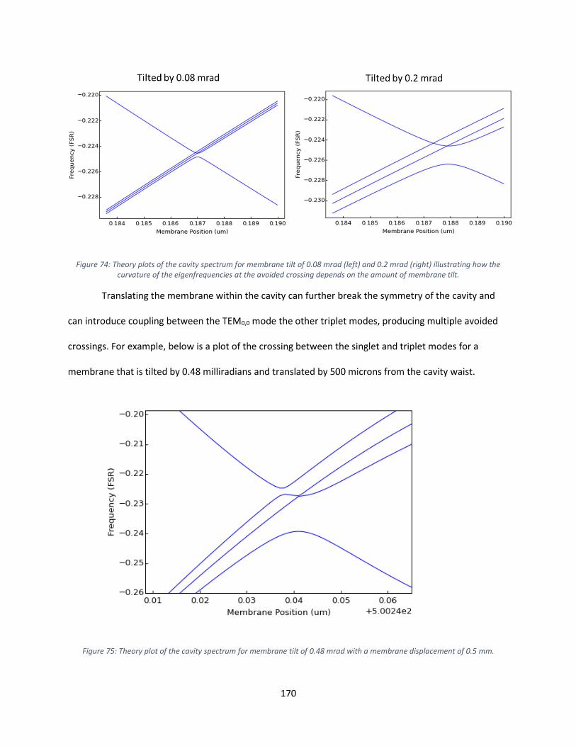
170

Figure 74: Theory plots of the cavity spectrum for membrane tilt of 0.08 mrad (left) and 0.2 mrad (right) illustrating how the curvature of the eigenfrequencies at the avoided crossing depends on the amount of membrane tilt.

Translating the membrane within the cavity can further break the symmetry of the cavity and

can introduce coupling between the TEM0,0 mode the other triplet modes, producing multiple avoided

crossings. For example, below is a plot of the crossing between the singlet and triplet modes for a

membrane that is tilted by 0.48 milliradians and translated by 500 microns from the cavity waist.

Figure 75: Theory plot of the cavity spectrum for membrane tilt of 0.48 mrad with a membrane displacement of 0.5 mm.

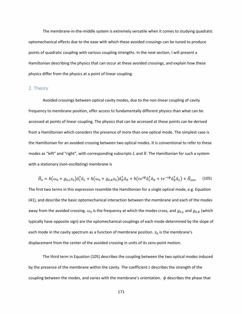
171

The membrane-in-the-middle system is extremely versatile when it comes to studying quadratic

optomechanical effects due to the ease with which these avoided crossings can be tuned to produce

points of quadratic coupling with various coupling strengths. In the next section, I will present a

Hamiltonian describing the physics that can occur at these avoided crossings, and explain how these

physics differ from the physics at a point of linear coupling.

2. Theory

Avoided crossings between optical cavity modes, due to the non-linear coupling of cavity

frequency to membrane position, offer access to fundamentally different physics than what can be

accessed at points of linear coupling. The physics that can be accessed at these points can be derived

from a Hamiltonian which considers the presence of more than one optical mode. The simplest case is

the Hamiltonian for an avoided crossing between two optical modes. It is conventional to refer to these

modes as “left” and “right”, with corresponding subscripts 𝐿 and 𝑅. The Hamiltonian for such a system

with a stationary (non-oscillating) membrane is

��0 = ℏ(𝜔0 + 𝑔0,𝐿𝑧0)��𝐿†��𝐿 + ℏ(𝜔0 + 𝑔0,𝑅𝑧0)��𝑅

† ��𝑅 + ℏ(𝑡𝑒𝑖𝜙��𝐿

†��𝑅 + 𝑡𝑒−𝑖𝜙��𝑅

† ��𝐿) + ��env (105)

The first two terms in this expression resemble the Hamiltonian for a single optical mode, e.g. Equation

(41), and describe the basic optomechanical interaction between the membrane and each of the modes

away from the avoided crossing. 𝜔0 is the frequency at which the modes cross, and 𝑔0,𝐿 and 𝑔0,𝑅 (which

typically have opposite sign) are the optomechanical couplings of each mode determined by the slope of

each mode in the cavity spectrum as a function of membrane position. 𝑧0 is the membrane’s

displacement from the center of the avoided crossing in units of its zero-point motion.

The third term in Equation (105) describes the coupling between the two optical modes induced

by the presence of the membrane within the cavity. The coefficient 𝑡 describes the strength of the

coupling between the modes, and varies with the membrane’s orientation. 𝜙 describes the phase that

172

would be acquired by a photon tunneling from one mode to another, which is analogous to saying that

each mode couples to the input drive with a unique phase, where the difference in phase between the

two modes is 𝜙. This Hamiltonian is conveniently expressed using vector notation to accommodate the

multiple optical modes:

��0 = ℏ��†(��𝑐(𝑧0))�� + ��env (106)

In Equation (106) �� = (��𝐿��𝑅), and ��† is its conjugate transpose. The matrix ��𝑐(𝑧0) describes the

optomechanical coupling between the modes as well as the tunneling rate between modes, and is

defined as

��𝑐(𝑧0) = (𝑔0,𝐿𝑧0 𝑡𝑒𝑖𝜙

𝑡𝑒−𝑖𝜙 𝑔0,𝑅𝑧0) (107)

The equations of motion of the system can now be written as

�� = −(��

2+ 𝑖��𝑐(𝑧0)) �� + √𝜅in

𝑎in (108)

�� and √𝜅𝑖𝑛 describe the bare linewidths of the modes and their input coupling rates, which need not be

equal:

�� = (𝜅𝐿 00 𝜅𝑅

) (109)

√𝜅in = (

√𝜅𝐿,in

√𝜅𝑅,in) (110)

𝑎in represents the external laser drive, which in a frame rotating at the laser frequency, can be written

as 𝑎in(𝑡) = 𝑎in𝑒−𝑖Δ𝑡. The steady state solution to Equation (108) is therefore

173

��(𝑡) = ��0𝑒−𝑖Δ𝑡

��0 = (��

2+ 𝑖(��𝑐(𝑧0) − Δ))

−1

√𝜅in 𝑎in

= ��𝑐[0]√𝜅in 𝑎in

(111)

The cavity susceptibility matrix ��𝑐[𝜔] ≡ (��

2+ 𝑖(��𝑐(𝑧0) − Δ − 𝜔))

−1

describes the response of

each cavity mode to optical drives of detuning Δ. (Scalars such as Δ are assumed to be multiplied by the

identity matrix, e.g. Δ ≡ Δ𝐼 = (Δ 00 Δ

).) With this, it is possible to express the reflected field amplitude

as a sum of the laser drive with the light that has leaked out of the cavity from each mode:

𝑎refl = 𝑎in −√𝜅in †��0 = 𝑎in (1 − √𝜅in

†��𝑐[0]√𝜅in ) (112)

Recall that so far, this formalism has dealt only with the case of a stationary membrane. To

consider the case of an oscillating membrane, additional mechanical terms must be added to yield the

complete the Hamiltonian:

�� = ℏ��†��𝑚 ���� + ℏ𝜔𝑚��†�� + ��0 (113)

The first term describes the interaction between the optical mode and the oscillatory motion of the

membrane. This interaction is not captured in the ℏ��†(��𝑐(𝑧0))�� term of Equation (106) because the

coupling of the laser to an arbitrary mechanical mode of the membrane is unlikely be as large as the

optomechanical coupling to static membrane displacements due to the curvature of the membrane

during oscillation. In fact, for certain modes, if the laser is aligned symmetrically about a nodal line of

the mechanical mode, the coupling could be as low as zero. Therefore, ��𝑚 represents the mode specific

optomechanical coupling. �� = ��† + �� represents the instantaneous displacement of the mode from

equilibrium. The second term in Equation (113) represents the energy of the mechanical mode, just as in

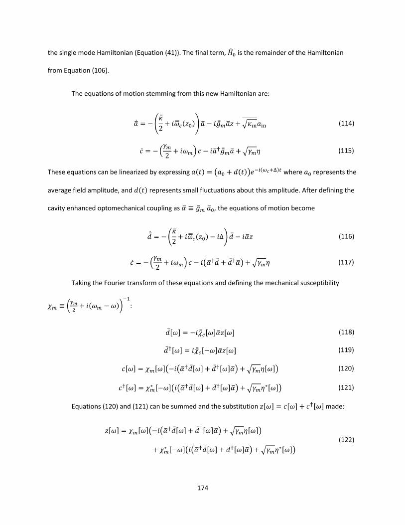
174

the single mode Hamiltonian (Equation (41)). The final term, ��0 is the remainder of the Hamiltonian

from Equation (106).

The equations of motion stemming from this new Hamiltonian are:

�� = −(��

2+ 𝑖��𝑐(𝑧0)) �� − 𝑖��𝑚��𝑧 + √𝜅in

𝑎in (114)

�� = −(𝛾𝑚2+ 𝑖𝜔𝑚) 𝑐 − 𝑖��

†��𝑚�� + √𝛾𝑚𝜂 (115)

These equations can be linearized by expressing 𝑎(𝑡) = (𝑎0 + 𝑑(𝑡))𝑒−𝑖(𝜔𝑐+Δ)𝑡 where 𝑎0 represents the

average field amplitude, and 𝑑(𝑡) represents small fluctuations about this amplitude. After defining the

cavity enhanced optomechanical coupling as �� ≡ ��𝑚 ��0, the equations of motion become

�� = −(��

2+ 𝑖��𝑐(𝑧0) − 𝑖Δ) �� − 𝑖��𝑧 (116)

�� = −(𝛾𝑚2+ 𝑖𝜔𝑚) 𝑐 − 𝑖(��

†�� + ��†��) + √𝛾𝑚𝜂 (117)

Taking the Fourier transform of these equations and defining the mechanical susceptibility

𝜒𝑚 ≡ (𝛾𝑚

2+ 𝑖(𝜔𝑚 −𝜔))

−1

:

��[𝜔] = −𝑖��𝑐[𝜔]��𝑧[𝜔] (118)

��†[𝜔] = 𝑖��𝑐[−𝜔]��𝑧[𝜔] (119)

𝑐[𝜔] = 𝜒𝑚[𝜔](−𝑖(��†��[𝜔] + ��†[𝜔]��) + √𝛾𝑚𝜂[𝜔]) (120)

𝑐†[𝜔] = 𝜒𝑚∗ [−𝜔](𝑖(��†��[𝜔] + ��†[𝜔]��) + √𝛾𝑚𝜂

∗[𝜔]) (121)

Equations (120) and (121) can be summed and the substitution 𝑧[𝜔] = 𝑐[𝜔] + 𝑐†[𝜔] made:

𝑧[𝜔] = 𝜒𝑚[𝜔](−𝑖(��

†��[𝜔] + ��†[𝜔]��) + √𝛾𝑚𝜂[𝜔])

+ 𝜒𝑚∗ [−𝜔](𝑖(��†��[𝜔] + ��†[𝜔]��) + √𝛾𝑚𝜂

∗[𝜔])

(122)

175

In the limit of high mechanical mode quality factor (𝜔𝑚 𝛾𝑚⁄ ≫ 1), the motion of the mechanical mode is

tightly localized around 𝜔 ≈ 𝜔𝑚. Using these two criteria, the mechanical susceptibility terms from

Equation (122) can be approximated as 𝜒𝑚[−𝜔] = (𝛾

2+ 𝑖(𝜔 + 𝜔𝑚))

−1

≈ (2𝑖𝜔𝑚)−1 and 𝜒𝑚[𝜔] =

(𝛾

2+ 𝑖(−𝜔 + 𝜔𝑚))

−1

≫ |𝜒𝑚∗ [−𝜔]|. Multiplying both sides of the equation by 𝜒𝑚

−1[𝜔], the 𝜒𝑚∗ [−𝜔] is

eliminated and the final result is achieved:

(𝜒𝑚−1[𝜔] + ��†(��𝑐[𝜔] − ��𝑐

†[−𝜔])��)𝑧[𝜔] = √𝛾𝑚𝜂[𝜔] (123)

In Equation (123), the bare mechanical susceptibility 𝜒𝑚−1[𝜔] is modified by the second term,

which is called the optomechanical self-energy, and is defined as follows:

Σ[𝜔] = −𝑖��†(��𝑐[𝜔] − ��𝑐†[−𝜔])�� (124)

The change in mechanical frequency and linewidth due to optical spring and damping therefore can be

easily computed from the self energy just as in the linear coupling case: 𝛿𝜔 = Re(Σ[𝜔𝑚]) and 𝛿𝛾 =

−2Im(Σ[𝜔𝑚]).

It is also possible to extend this theory to describe a system with more than two interacting

optical modes. This is important because all Hermite Gauss optical modes other than the TEM0,0 exhibit

degeneracy. Therefore, any complete theory of the optomechanics at an avoided crossing must also

consider the effects of the nearby nearly degenerate modes. The extension of the theory to account for

additional modes is accomplished with the following substitutions.

�� → (

��𝐿��𝑅1��𝑅2⋮

) (125)

176

√𝜅𝑖𝑛 →

(

√𝜅𝐿,𝑖𝑛

√𝜅𝑅1,𝑖𝑛

√𝜅𝑅2,𝑖𝑛⋮ )

(126)

�� → (

𝜅𝐿𝜅𝑅1

𝜅𝑅2⋱

) (127)

��𝑐(𝑧0) →

(

𝑔0,𝐿𝑧0 𝑡1𝑒𝑖𝜙1 𝑡2𝑒

𝑖𝜙2 ⋯

𝑡1𝑒−𝑖𝜙1 𝑔0,𝑅1𝑧0

𝑡2𝑒−𝑖𝜙2 𝜎2 + 𝑔0,𝑅2𝑧0⋮ ⋱)

(128)

In Equations (125)-(128), subscripts 𝐿 and 𝑅1 are the modes from the original two-mode model. The

additional nearly degenerate modes are represented by subscripts {𝑅2,… }. Equation (128) accounts for

the fact that these additional modes are not fully degenerate with the terms {𝜎2, … }, which represent

the frequency difference between modes {𝑅2,… } and the frequency of the avoided crossing between

modes 𝐿 and 𝑅1. The terms 𝑡𝑛 and 𝜙𝑛 represent the coupling strength and phase acquired by photons

tunneling from mode 𝐿 to mode 𝑅𝑛.

The full algebraic expressions for the spring and damping are quite complicated to write out,

even for the two-mode case, but numerical simulations can be easily used to predict the behavior of the

optomechanical system for any number of modes. Figure 76 shows a plot of the optical spring and

damping for a three mode system similar to the actual system we measured. (The parameters used to

generate this theory plot are given in columns II and III of Table 2 later in this chapter.)

177

Figure 76: Theory plots of optical spring (left) and optical damping (right) for a system consisting of three optical modes forming two avoided crossings.

In Figure 76, it is clear that away from the avoided crossings, the system exhibits behavior

typical of regular linear optomechanics. When red-detuned from the cavity resonance, the optical mode

experiences positive damping and a negative spring shift. When blue detuned, the damping is negative

and the spring shift is positive. At an avoided crossing, the spring shift occurs when the laser is on

resonance rather than when it is detuned, and the damping becomes very small.

The reason why the mechanical mode responds like this near the avoided crossings can be

understood by rewriting the Hamiltonian in the basis of the cavity eigenmodes at the avoided crossing.

In this basis, at the avoided crossing, rather than two coupled modes that respond linearly to changes in

position of the membrane, there are two modes that respond quadratically to the position of the

membrane. A qualitative description of the system’s dynamics can be extracted by looking at a

Hamiltonian that considers only one of the two modes. Such a Hamiltonian can be written as: 37

�� ≈ ℏ (𝜔𝑐 +1

2𝑧zpf2 𝜔𝑐

′′(��† + ��)2) ��†�� + ℏ𝜔𝑚��

†�� (129)

In Equation (129), 𝜔𝑐′′ represents the second derivative of cavity mode’s resonant frequency

with respect to membrane position. In the rotating wave approximation, this Hamiltonian becomes:

178

�� ≈ ℏ(𝜔𝑐 + 𝑧zpf2 𝜔𝑐

′′ (��†�� +1

2)) ��†�� + ℏ𝜔𝑚��

†�� (130)

Defining the quadratic optomechanical coupling strength 𝑔2 ≡ 𝜔𝑐′′𝑧zpf

2 the terms in Equation

(130) can be regrouped into a form that makes the origin of the spring shift at the avoided crossing in

Figure 76 clear:

�� = ℏ𝜔𝑐��†�� +

1

2𝑔2��

†�� + ℏ(𝜔𝑚 + 𝑔2��†��)��†�� (131)

From Equation (131) it is clear that the quadratic coupling leads to a mechanical frequency shift

per photon of light in the cavity. Therefore, at a point of quadratic coupling, the magnitude of the spring

shift is maximized when the laser is on resonance with the cavity and the intracavity photon number

��†�� is maximized. The lack of optical damping at a point of quadratic coupling is also evident from

Equation (131). Since the Hamiltonian has no dependence on 𝜔𝑐′ , the net radiation pressure force acting

on the membrane is zero. Thus, there can be no optical damping. It should be noted however that this

simplified Hamiltonian does not capture the full behavior of the system. Damping can still occur through

two phonon Raman processes that are not considered in the linearized Hamiltonian. Additionally, this

Hamiltonian does not consider the presence of the second cavity eigenmode – as the gap between the

two modes at the avoided crossing approaches the linewidth of the modes, it is no longer appropriate to

approximate them as non-interacting quadratically coupled modes in the Hamiltonian, and the optical

damping rate can become non-zero. 46

3. Experimental Setup

The experimental setup of the quadratic optomechanics experiment was overall quite similar to

the setup used for ground state cooling, though there were significant differences in the optical setup

outside of the cryostat, and a different membrane and cryogenic cavity were used.

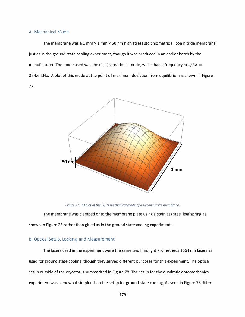
179

A. Mechanical Mode

The membrane was a 1 mm × 1 mm × 50 nm high stress stoichiometric silicon nitride membrane

just as in the ground state cooling experiment, though it was produced in an earlier batch by the

manufacturer. The mode used was the (1, 1) vibrational mode, which had a frequency 𝜔𝑚 2𝜋⁄ =

354.6 kHz. A plot of this mode at the point of maximum deviation from equilibrium is shown in Figure

77.

Figure 77: 3D plot of the (1, 1) mechanical mode of a silicon nitride membrane.

The membrane was clamped onto the membrane plate using a stainless steel leaf spring as

shown in Figure 25 rather than glued as in the ground state cooling experiment.

B. Optical Setup, Locking, and Measurement

The lasers used in the experiment were the same two Innolight Prometheus 1064 nm lasers as

used for ground state cooling, though they served different purposes for this experiment. The optical

setup outside of the cryostat is summarized in Figure 78. The setup for the quadratic optomechanics

experiment was somewhat simpler than the setup for ground state cooling. As seen in Figure 78, filter

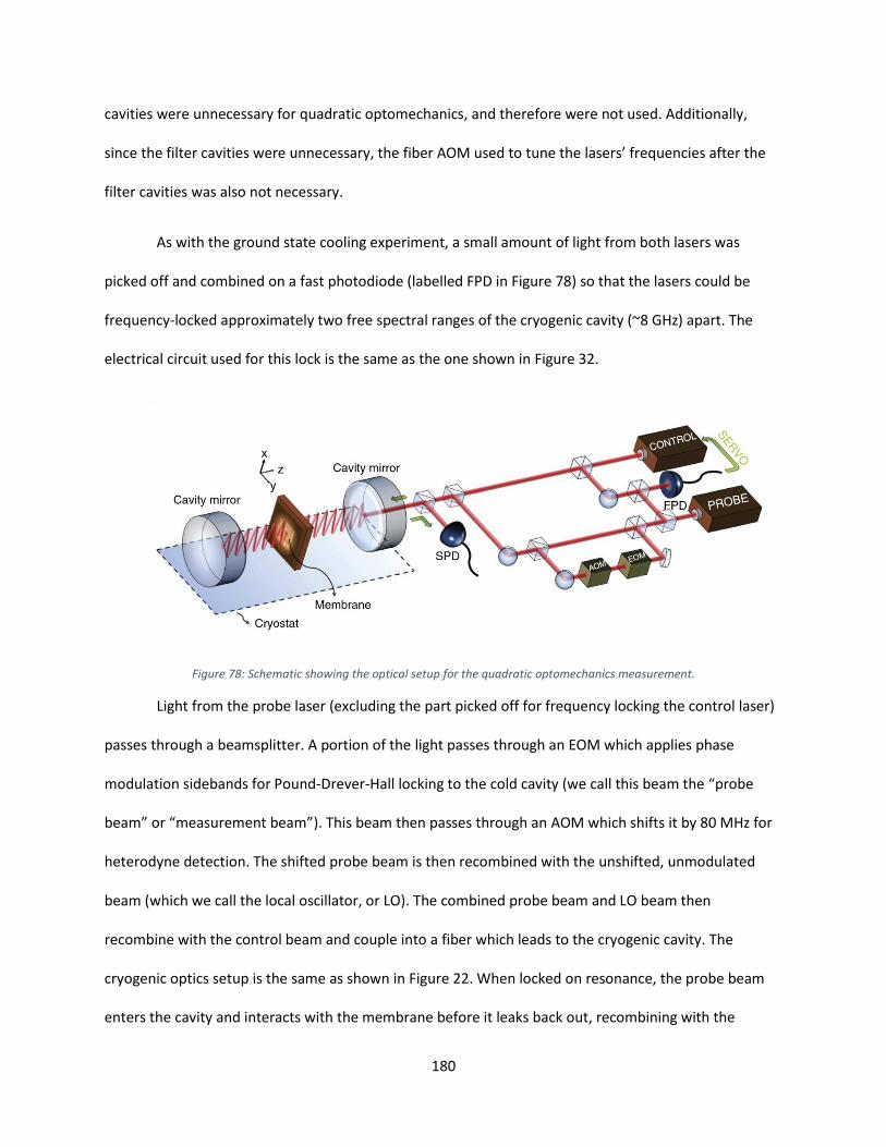
180

cavities were unnecessary for quadratic optomechanics, and therefore were not used. Additionally,

since the filter cavities were unnecessary, the fiber AOM used to tune the lasers’ frequencies after the

filter cavities was also not necessary.

As with the ground state cooling experiment, a small amount of light from both lasers was

picked off and combined on a fast photodiode (labelled FPD in Figure 78) so that the lasers could be

frequency-locked approximately two free spectral ranges of the cryogenic cavity (~8 GHz) apart. The

electrical circuit used for this lock is the same as the one shown in Figure 32.

Figure 78: Schematic showing the optical setup for the quadratic optomechanics measurement.

Light from the probe laser (excluding the part picked off for frequency locking the control laser)

passes through a beamsplitter. A portion of the light passes through an EOM which applies phase

modulation sidebands for Pound-Drever-Hall locking to the cold cavity (we call this beam the “probe

beam” or “measurement beam”). This beam then passes through an AOM which shifts it by 80 MHz for

heterodyne detection. The shifted probe beam is then recombined with the unshifted, unmodulated

beam (which we call the local oscillator, or LO). The combined probe beam and LO beam then

recombine with the control beam and couple into a fiber which leads to the cryogenic cavity. The

cryogenic optics setup is the same as shown in Figure 22. When locked on resonance, the probe beam

enters the cavity and interacts with the membrane before it leaks back out, recombining with the

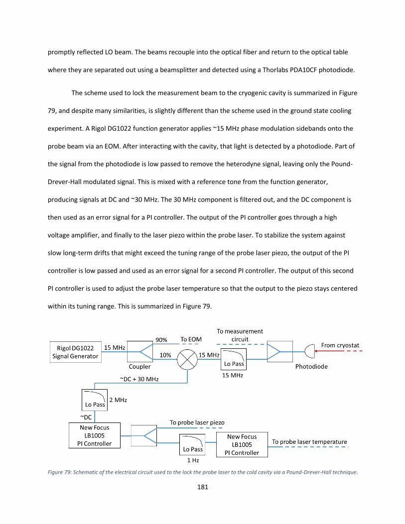
181

promptly reflected LO beam. The beams recouple into the optical fiber and return to the optical table

where they are separated out using a beamsplitter and detected using a Thorlabs PDA10CF photodiode.

The scheme used to lock the measurement beam to the cryogenic cavity is summarized in Figure

79, and despite many similarities, is slightly different than the scheme used in the ground state cooling

experiment. A Rigol DG1022 function generator applies ~15 MHz phase modulation sidebands onto the

probe beam via an EOM. After interacting with the cavity, that light is detected by a photodiode. Part of

the signal from the photodiode is low passed to remove the heterodyne signal, leaving only the Pound-

Drever-Hall modulated signal. This is mixed with a reference tone from the function generator,

producing signals at DC and ~30 MHz. The 30 MHz component is filtered out, and the DC component is

then used as an error signal for a PI controller. The output of the PI controller goes through a high

voltage amplifier, and finally to the laser piezo within the probe laser. To stabilize the system against

slow long-term drifts that might exceed the tuning range of the probe laser piezo, the output of the PI

controller is low passed and used as an error signal for a second PI controller. The output of this second

PI controller is used to adjust the probe laser temperature so that the output to the piezo stays centered

within its tuning range. This is summarized in Figure 79.

Figure 79: Schematic of the electrical circuit used to the lock the probe laser to the cold cavity via a Pound-Drever-Hall technique.

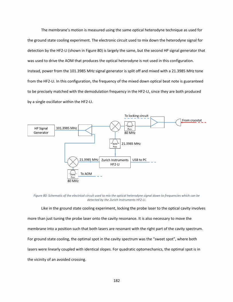
182

The membrane’s motion is measured using the same optical heterodyne technique as used for

the ground state cooling experiment. The electronic circuit used to mix down the heterodyne signal for

detection by the HF2-LI (shown in Figure 80) is largely the same, but the second HP signal generator that

was used to drive the AOM that produces the optical heterodyne is not used in this configuration.

Instead, power from the 101.3985 MHz signal generator is split off and mixed with a 21.3985 MHz tone

from the HF2-LI. In this configuration, the frequency of the mixed down optical beat note is guaranteed

to be precisely matched with the demodulation frequency in the HF2-LI, since they are both produced

by a single oscillator within the HF2-LI.

Figure 80: Schematic of the electrical circuit used to mix the optical heterodyne signal down to frequencies which can be detected by the Zurich Instruments HF2-LI.

Like in the ground state cooling experiment, locking the probe laser to the optical cavity involves

more than just tuning the probe laser onto the cavity resonance. It is also necessary to move the

membrane into a position such that both lasers are resonant with the right part of the cavity spectrum.

For ground state cooling, the optimal spot in the cavity spectrum was the “sweet spot”, where both

lasers were linearly coupled with identical slopes. For quadratic optomechanics, the optimal spot is in

the vicinity of an avoided crossing.

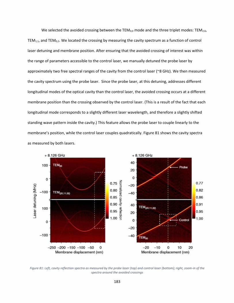
183

We selected the avoided crossing between the TEM0,0 mode and the three triplet modes: TEM2,0,

TEM1,1, and TEM0,2. We located the crossing by measuring the cavity spectrum as a function of control

laser detuning and membrane position. After ensuring that the avoided crossing of interest was within

the range of parameters accessible to the control laser, we manually detuned the probe laser by

approximately two free spectral ranges of the cavity from the control laser (~8 GHz). We then measured

the cavity spectrum using the probe laser. Since the probe laser, at this detuning, addresses different

longitudinal modes of the optical cavity than the control laser, the avoided crossing occurs at a different

membrane position than the crossing observed by the control laser. (This is a result of the fact that each

longitudinal mode corresponds to a slightly different laser wavelength, and therefore a slightly shifted

standing wave pattern inside the cavity.) This feature allows the probe laser to couple linearly to the

membrane’s position, while the control laser couples quadratically. Figure 81 shows the cavity spectra

as measured by both lasers.

Figure 81: Left, cavity reflection spectra as measured by the probe laser (top) and control laser (bottom); right, zoom-in of the spectra around the avoided crossings

184

C. Characterizing Parameters

Calibrating the axes of the spectra in Figure 81 into units of frequency (for the y-axis) and

displacement (for the x-axis) is the first step in characterizing experimental parameters to aid in

analyzing results of measurements of the optomechanical dynamics of the system. The laser frequency

and the membrane position are controlled by voltages to piezo actuators in the laser, and beneath the

membrane, respectively. For the laser frequency, the piezo voltage-to-frequency conversion factor can

be found by applying phase modulation sidebands at a known frequency using an EOM and measuring

the piezo voltage difference necessary to shift the laser frequency such that first one, then the other

sideband is on resonance with the cavity. This is the same procedure used to initially characterize the

cavity linewidth in the ground state cooling measurement. See e.g., Figure 44.

For the membrane position, we calibrated the piezo voltage into units of displacement by

measuring the difference in piezo voltage needed to move the membrane from a node of the cavity field

to an antinode. Since nodes and antinodes should be separated from each other by a distance 𝜆/4 and

can be easily identified in the cavity spectrum as points of minimum and maximum resonance frequency

(as shown in, e.g. Figure 9) this is a simple measurement to make by inspection of the cavity spectra.

The theory of multiple optical modes described at the beginning of this chapter should fully

describe all aspects of the cavity spectrum in the vicinity of the avoided crossing. Therefore, once the

measured cavity spectrum has been calibrated into units of laser frequency and membrane

displacement, the spectrum itself can be used to characterize parameters in the theory. For example,

the linewidth of each of the optical modes can be determined by fitting each vertical slice through the

two-dimensional spectrum to a sum of Lorentzian lineshapes (with each representing one mode.) This

process is shown in Figure 82, where the two modes that couple in the avoided crossing have been fit.

185

Figure 82: Left, zoom-in of the cavity spectrum around the avoided crossing. Right, a vertical slice of the two-dimensional spectrum, indicated on the left by the dashed white line. The red line is a fit to a sum of two Lorentzians plus a sinusoidal

background, which comes from interference caused by reflections in the beam path.

From the fits to the slices of the two-dimensional cavity spectrum we extract the mode

linewidths 𝜅, and the coupling rate of each mode to the external field through the input mirror 𝜅in. The

procedure for extracting 𝜅in here is the same as it was to extract 𝜅in in the ground state cooling

measurement. Since the laser is primarily mode-matched to the TEM0,0, the fractional reflection dip of

the fainter mode in Figure 82 is small enough that it is difficult to fit above the sinusoidal background in

the sweep. (The sinusoidal background is caused by back-reflections within the beam path causing

periodic interference as the laser frequency is swept.) To improve the accuracy of fitting such faintly

coupled modes, a series of fits is performed to slices at different membrane positions, and the fit results

of parameters such as 𝜅 and 𝜅in are averaged.

For the particular avoided crossing shown in Figure 82, one of the triplet modes couples to the

TEM0,0 mode. However, depending on the membrane’s tip and tilt in the cavity, there are configurations

in which more than one mode can couple. In these cases, additional modes can be included in the fits to

vertical slices of the cavity spectrum.

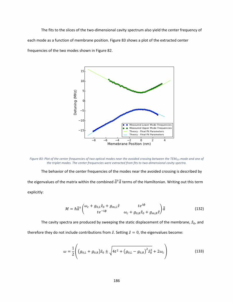
186

The fits to the slices of the two-dimensional cavity spectrum also yield the center frequency of

each mode as a function of membrane position. Figure 83 shows a plot of the extracted center

frequencies of the two modes shown in Figure 82.

Figure 83: Plot of the center frequencies of two optical modes near the avoided crossing between the TEM0,0 mode and one of the triplet modes. The center frequencies were extracted from fits to two-dimensional cavity spectra.

The behavior of the center frequencies of the modes near the avoided crossing is described by

the eigenvalues of the matrix within the combined ��†�� terms of the Hamiltonian. Writing out this term

explicitly:

𝑀 = ℏ��† (𝜔𝑐 + 𝑔0,𝐿��0 + 𝑔𝑚,𝐿�� 𝑡𝑒𝑖𝜙

𝑡𝑒−𝑖𝜙 𝜔𝑐 + 𝑔0,𝑅��0 + 𝑔𝑚,𝑅��) �� (132)

The cavity spectra are produced by sweeping the static displacement of the membrane, ��0, and

therefore they do not include contributions from ��. Setting �� = 0, the eigenvalues become:

𝜔 =1

2((𝑔0,𝐿 + 𝑔0,𝑅)��0 ±√4𝑡

2 + (𝑔0,𝐿 − 𝑔0,𝑅)2��02 + 2𝜔𝑐) (133)

187

From Equation (133) it is clear that for 𝑧0 ≫ 𝑡, the eigenvalues are roughly the same as they

would be if the modes were noninteracting. Near the avoided crossing, however, 𝑧0 ≈ 0, and each

mode is shifted by an amount equal to 𝑡. The values of 𝑔0,𝐿 and 𝑔0,𝑅 can therefore be extracted from

the slope of the modes’ resonant frequencies away from the avoided crossing, while the value of 𝑡 can

be extracted from the size of the gap between the two modes at the crossing. For better precision in

measuring 𝑡, it is useful to expand the eigenvalues in a Taylor series to second order in ��0 and fit the

modes around the avoided crossing with a quadratic function to determine the second-order coefficient

in the Taylor series. It is then possible to extract 𝑡 from this coefficient. We used this more precise

method whenever possible to extract the value of 𝑡. This method also has the advantage of revealing

the quadratic coupling strength 𝜔𝑐′′, which is simply the coefficient of the quadratic term in the Taylor

expansion.

The value of 𝜙, the phase difference between the two modes at the avoided crossing, affects

the interference between the modes when 𝑧0 ≈ 0. It can therefore be extracted by comparing the

relative laser coupling strengths of the hybridized modes (indicated by their reflection dips) at the

avoided crossing. Figure 84 shows theory plots of the cavity spectrum, zoomed in on the avoided

crossing for various values of 𝜙.

Figure 84: Theory plots of the cavity spectrum near the avoided crossing as a function of the tunneling phase 𝜙.

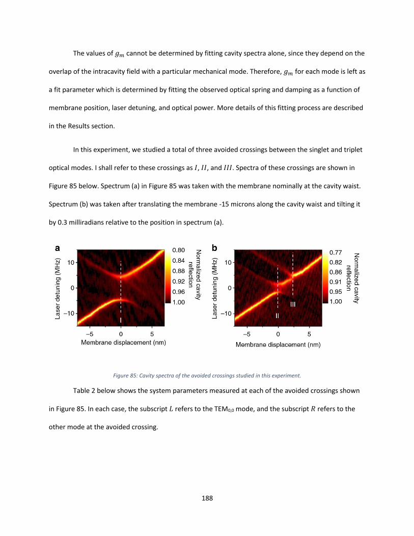
188

The values of 𝑔𝑚 cannot be determined by fitting cavity spectra alone, since they depend on the

overlap of the intracavity field with a particular mechanical mode. Therefore, 𝑔𝑚 for each mode is left as

a fit parameter which is determined by fitting the observed optical spring and damping as a function of

membrane position, laser detuning, and optical power. More details of this fitting process are described

in the Results section.

In this experiment, we studied a total of three avoided crossings between the singlet and triplet

optical modes. I shall refer to these crossings as 𝐼, 𝐼𝐼, and 𝐼𝐼𝐼. Spectra of these crossings are shown in

Figure 85 below. Spectrum (a) in Figure 85 was taken with the membrane nominally at the cavity waist.

Spectrum (b) was taken after translating the membrane -15 microns along the cavity waist and tilting it

by 0.3 milliradians relative to the position in spectrum (a).

Figure 85: Cavity spectra of the avoided crossings studied in this experiment.

Table 2 below shows the system parameters measured at each of the avoided crossings shown

in Figure 85. In each case, the subscript 𝐿 refers to the TEM0,0 mode, and the subscript 𝑅 refers to the

other mode at the avoided crossing.

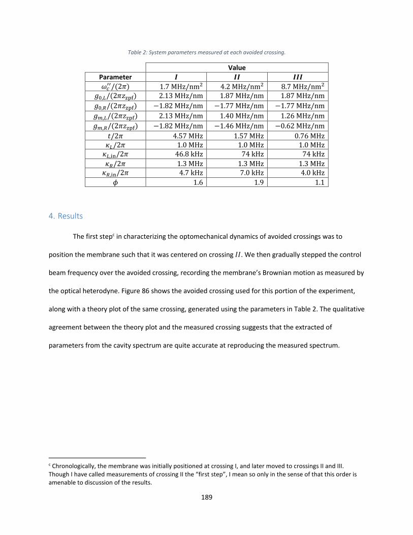
189

Table 2: System parameters measured at each avoided crossing.

Value

Parameter 𝑰 𝑰𝑰 𝑰𝑰𝑰 𝜔𝑐′′/(2𝜋) 1.7 MHz/nm2 4.2 MHz/nm2 8.7 MHz/nm2

𝑔0,𝐿/(2𝜋𝑧zpf) 2.13 MHz/nm 1.87 MHz/nm 1.87 MHz/nm

𝑔0,𝑅/(2𝜋𝑧zpf) −1.82 MHz/nm −1.77 MHz/nm −1.77 MHz/nm

𝑔𝑚,𝐿/(2𝜋𝑧zpf) 2.13 MHz/nm 1.40 MHz/nm 1.26 MHz/nm

𝑔𝑚,𝑅/(2𝜋𝑧zpf) −1.82 MHz/nm −1.46 MHz/nm −0.62 MHz/nm

𝑡/2𝜋 4.57 MHz 1.57 MHz 0.76 MHz 𝜅𝐿/2𝜋 1.0 MHz 1.0 MHz 1.0 MHz 𝜅𝐿,in/2𝜋 46.8 kHz 74 kHz 74 kHz

𝜅𝑅/2𝜋 1.3 MHz 1.3 MHz 1.3 MHz 𝜅𝑅,in/2𝜋 4.7 kHz 7.0 kHz 4.0 kHz

𝜙 1.6 1.9 1.1

4. Results

The first stepc in characterizing the optomechanical dynamics of avoided crossings was to

position the membrane such that it was centered on crossing 𝐼𝐼. We then gradually stepped the control

beam frequency over the avoided crossing, recording the membrane’s Brownian motion as measured by

the optical heterodyne. Figure 86 shows the avoided crossing used for this portion of the experiment,

along with a theory plot of the same crossing, generated using the parameters in Table 2. The qualitative

agreement between the theory plot and the measured crossing suggests that the extracted of

parameters from the cavity spectrum are quite accurate at reproducing the measured spectrum.

c Chronologically, the membrane was initially positioned at crossing I, and later moved to crossings II and III. Though I have called measurements of crossing II the “first step”, I mean so only in the sense of that this order is amenable to discussion of the results.

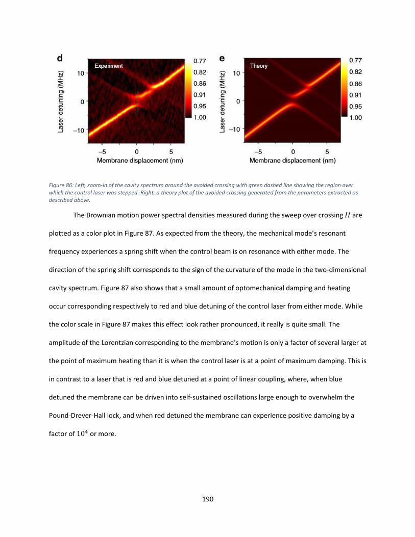
190

Figure 86: Left, zoom-in of the cavity spectrum around the avoided crossing with green dashed line showing the region over which the control laser was stepped. Right, a theory plot of the avoided crossing generated from the parameters extracted as described above.

The Brownian motion power spectral densities measured during the sweep over crossing 𝐼𝐼 are

plotted as a color plot in Figure 87. As expected from the theory, the mechanical mode’s resonant

frequency experiences a spring shift when the control beam is on resonance with either mode. The

direction of the spring shift corresponds to the sign of the curvature of the mode in the two-dimensional

cavity spectrum. Figure 87 also shows that a small amount of optomechanical damping and heating

occur corresponding respectively to red and blue detuning of the control laser from either mode. While

the color scale in Figure 87 makes this effect look rather pronounced, it really is quite small. The

amplitude of the Lorentzian corresponding to the membrane’s motion is only a factor of several larger at

the point of maximum heating than it is when the control laser is at a point of maximum damping. This is

in contrast to a laser that is red and blue detuned at a point of linear coupling, where, when blue

detuned the membrane can be driven into self-sustained oscillations large enough to overwhelm the

Pound-Drever-Hall lock, and when red detuned the membrane can experience positive damping by a

factor of 104 or more.

191

Figure 87: Left, color plot of Brownian motion power spectral densities of the membrane measured as the control laser was stepped across the avoided crossing. Right, color plot of the Brownian motion as predicted by theory.

After confirming that the Brownian motion behaves as expected right at the avoided crossing,

we repeated the measurement at a series of membrane positions. This allowed us to observe the

transition from traditional single-mode optomechanics to the multimode effects that occur at the

avoided crossing. We picked ten different membrane positions around crossing 𝐼𝐼 and stepped the

control laser frequency over both of the optical modes at each membrane position. The membrane

positions selected ranged from 0.96 nm to the left of the crossing to 1.38 nm to the right of the crossing.

The laser power was fixed at 80 μW incident on the cavity for the entire measurement. At each

membrane position, the laser was swept over a frequency range of about 15 MHz, centered right in the

middle of the two modes. Figure 88 shows the membrane positions and laser frequency ranges probed.

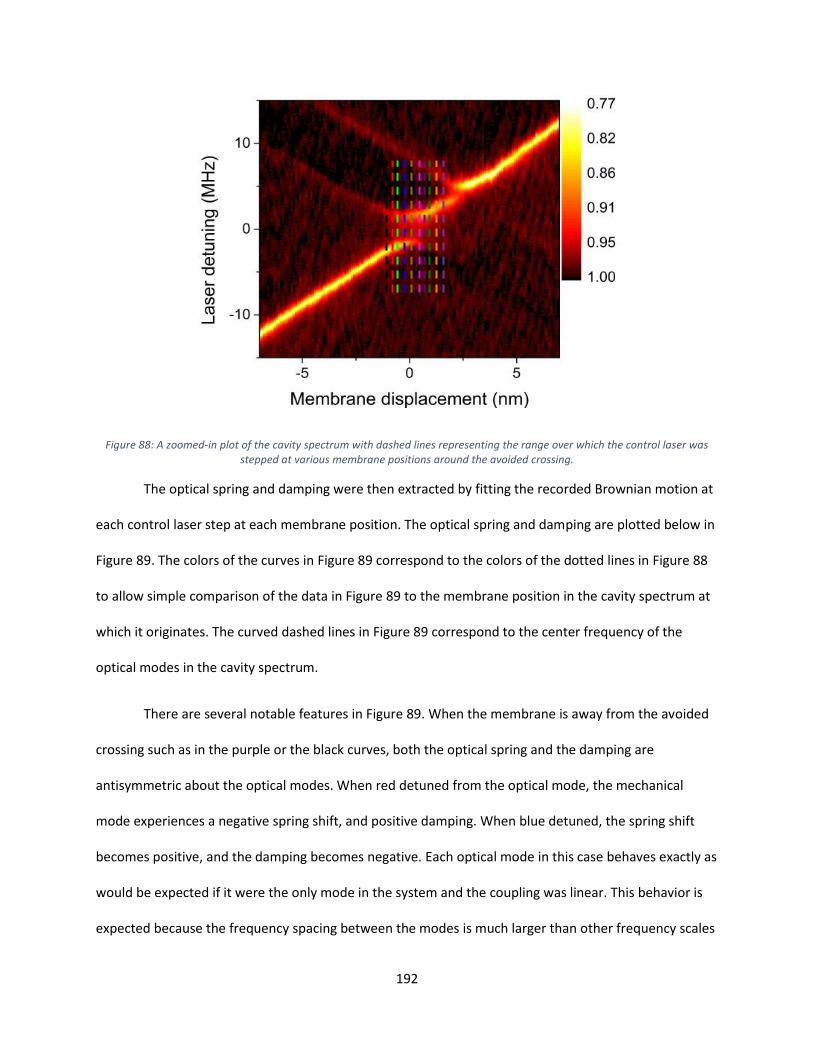
192

Figure 88: A zoomed-in plot of the cavity spectrum with dashed lines representing the range over which the control laser was stepped at various membrane positions around the avoided crossing.

The optical spring and damping were then extracted by fitting the recorded Brownian motion at

each control laser step at each membrane position. The optical spring and damping are plotted below in

Figure 89. The colors of the curves in Figure 89 correspond to the colors of the dotted lines in Figure 88

to allow simple comparison of the data in Figure 89 to the membrane position in the cavity spectrum at

which it originates. The curved dashed lines in Figure 89 correspond to the center frequency of the

optical modes in the cavity spectrum.

There are several notable features in Figure 89. When the membrane is away from the avoided

crossing such as in the purple or the black curves, both the optical spring and the damping are

antisymmetric about the optical modes. When red detuned from the optical mode, the mechanical

mode experiences a negative spring shift, and positive damping. When blue detuned, the spring shift

becomes positive, and the damping becomes negative. Each optical mode in this case behaves exactly as

would be expected if it were the only mode in the system and the coupling was linear. This behavior is

expected because the frequency spacing between the modes is much larger than other frequency scales

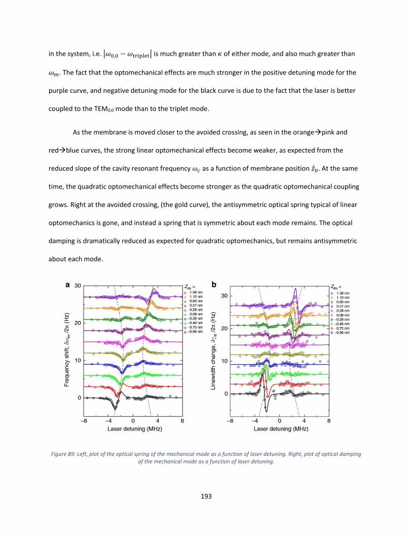
193

in the system, i.e. |𝜔0,0 −𝜔triplet| is much greater than 𝜅 of either mode, and also much greater than

𝜔𝑚. The fact that the optomechanical effects are much stronger in the positive detuning mode for the

purple curve, and negative detuning mode for the black curve is due to the fact that the laser is better

coupled to the TEM0,0 mode than to the triplet mode.

As the membrane is moved closer to the avoided crossing, as seen in the orangepink and

redblue curves, the strong linear optomechanical effects become weaker, as expected from the

reduced slope of the cavity resonant frequency 𝜔𝑐 as a function of membrane position ��0. At the same

time, the quadratic optomechanical effects become stronger as the quadratic optomechanical coupling

grows. Right at the avoided crossing, (the gold curve), the antisymmetric optical spring typical of linear

optomechanics is gone, and instead a spring that is symmetric about each mode remains. The optical

damping is dramatically reduced as expected for quadratic optomechanics, but remains antisymmetric

about each mode.

Figure 89: Left, plot of the optical spring of the mechanical mode as a function of laser detuning. Right, plot of optical damping of the mechanical mode as a function of laser detuning.

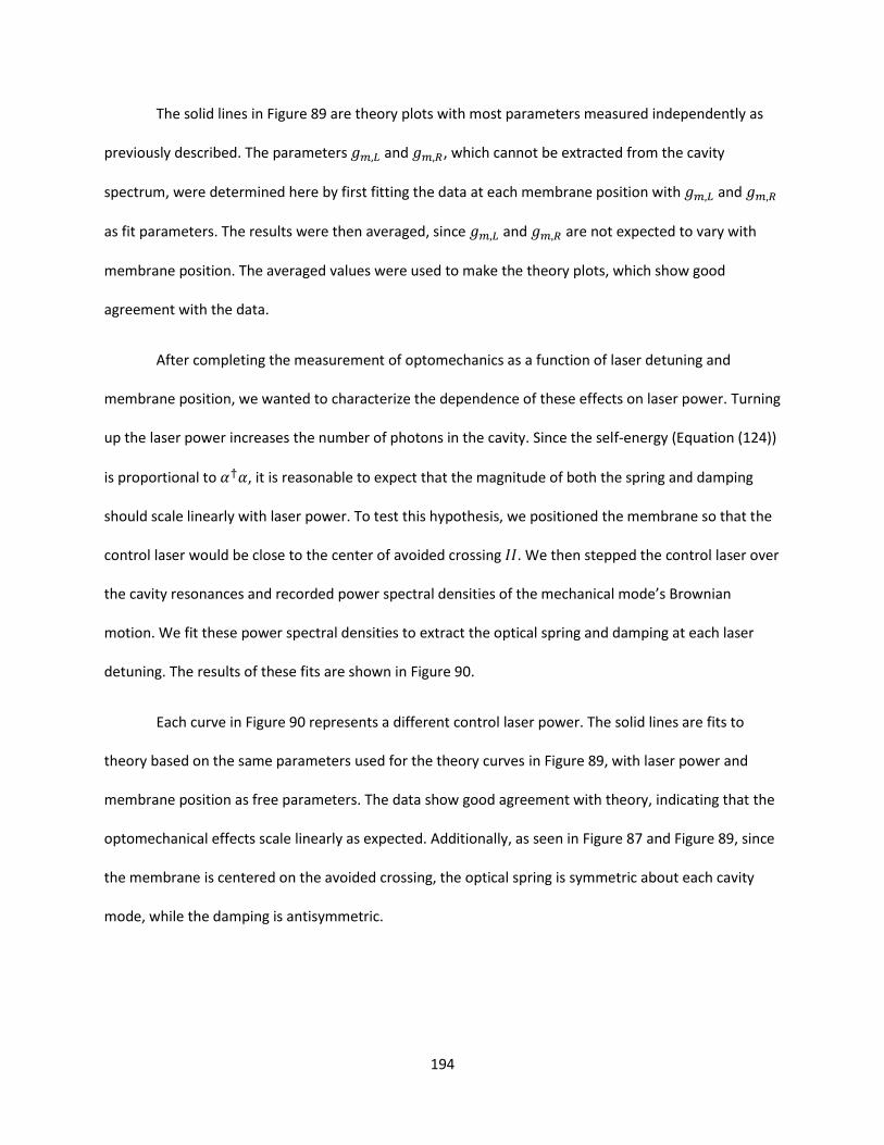
194

The solid lines in Figure 89 are theory plots with most parameters measured independently as

previously described. The parameters 𝑔𝑚,𝐿 and 𝑔𝑚,𝑅, which cannot be extracted from the cavity

spectrum, were determined here by first fitting the data at each membrane position with 𝑔𝑚,𝐿 and 𝑔𝑚,𝑅

as fit parameters. The results were then averaged, since 𝑔𝑚,𝐿 and 𝑔𝑚,𝑅 are not expected to vary with

membrane position. The averaged values were used to make the theory plots, which show good

agreement with the data.

After completing the measurement of optomechanics as a function of laser detuning and

membrane position, we wanted to characterize the dependence of these effects on laser power. Turning

up the laser power increases the number of photons in the cavity. Since the self-energy (Equation (124))

is proportional to 𝛼†𝛼, it is reasonable to expect that the magnitude of both the spring and damping

should scale linearly with laser power. To test this hypothesis, we positioned the membrane so that the

control laser would be close to the center of avoided crossing 𝐼𝐼. We then stepped the control laser over

the cavity resonances and recorded power spectral densities of the mechanical mode’s Brownian

motion. We fit these power spectral densities to extract the optical spring and damping at each laser

detuning. The results of these fits are shown in Figure 90.

Each curve in Figure 90 represents a different control laser power. The solid lines are fits to

theory based on the same parameters used for the theory curves in Figure 89, with laser power and

membrane position as free parameters. The data show good agreement with theory, indicating that the

optomechanical effects scale linearly as expected. Additionally, as seen in Figure 87 and Figure 89, since

the membrane is centered on the avoided crossing, the optical spring is symmetric about each cavity

mode, while the damping is antisymmetric.

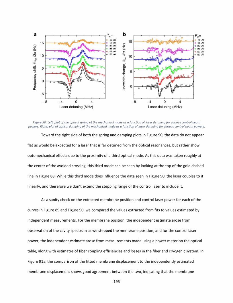
195

Figure 90: Left, plot of the optical spring of the mechanical mode as a function of laser detuning for various control beam powers. Right, plot of optical damping of the mechanical mode as a function of laser detuning for various control beam powers.

Toward the right side of both the spring and damping plots in Figure 90, the data do not appear

flat as would be expected for a laser that is far detuned from the optical resonances, but rather show

optomechanical effects due to the proximity of a third optical mode. As this data was taken roughly at

the center of the avoided crossing, this third mode can be seen by looking at the top of the gold dashed

line in Figure 88. While this third mode does influence the data seen in Figure 90, the laser couples to it

linearly, and therefore we don’t extend the stepping range of the control laser to include it.

As a sanity check on the extracted membrane position and control laser power for each of the

curves in Figure 89 and Figure 90, we compared the values extracted from fits to values estimated by

independent measurements. For the membrane position, the independent estimate arose from

observation of the cavity spectrum as we stepped the membrane position, and for the control laser

power, the independent estimate arose from measurements made using a power meter on the optical

table, along with estimates of fiber coupling efficiencies and losses in the fiber and cryogenic system. In

Figure 91a, the comparison of the fitted membrane displacement to the independently estimated

membrane displacement shows good agreement between the two, indicating that the membrane

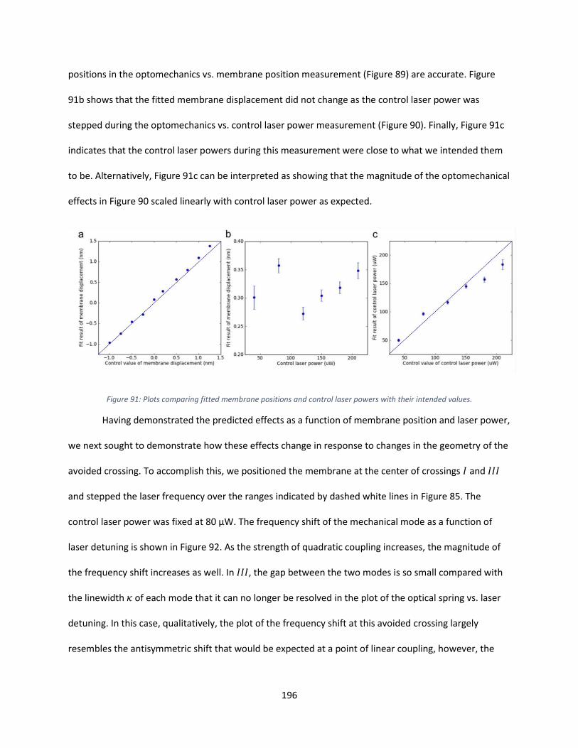
196

positions in the optomechanics vs. membrane position measurement (Figure 89) are accurate. Figure

91b shows that the fitted membrane displacement did not change as the control laser power was

stepped during the optomechanics vs. control laser power measurement (Figure 90). Finally, Figure 91c

indicates that the control laser powers during this measurement were close to what we intended them

to be. Alternatively, Figure 91c can be interpreted as showing that the magnitude of the optomechanical

effects in Figure 90 scaled linearly with control laser power as expected.

Figure 91: Plots comparing fitted membrane positions and control laser powers with their intended values.

Having demonstrated the predicted effects as a function of membrane position and laser power,

we next sought to demonstrate how these effects change in response to changes in the geometry of the

avoided crossing. To accomplish this, we positioned the membrane at the center of crossings 𝐼 and 𝐼𝐼𝐼

and stepped the laser frequency over the ranges indicated by dashed white lines in Figure 85. The

control laser power was fixed at 80 μW. The frequency shift of the mechanical mode as a function of

laser detuning is shown in Figure 92. As the strength of quadratic coupling increases, the magnitude of

the frequency shift increases as well. In 𝐼𝐼𝐼, the gap between the two modes is so small compared with

the linewidth 𝜅 of each mode that it can no longer be resolved in the plot of the optical spring vs. laser

detuning. In this case, qualitatively, the plot of the frequency shift at this avoided crossing largely

resembles the antisymmetric shift that would be expected at a point of linear coupling, however, the

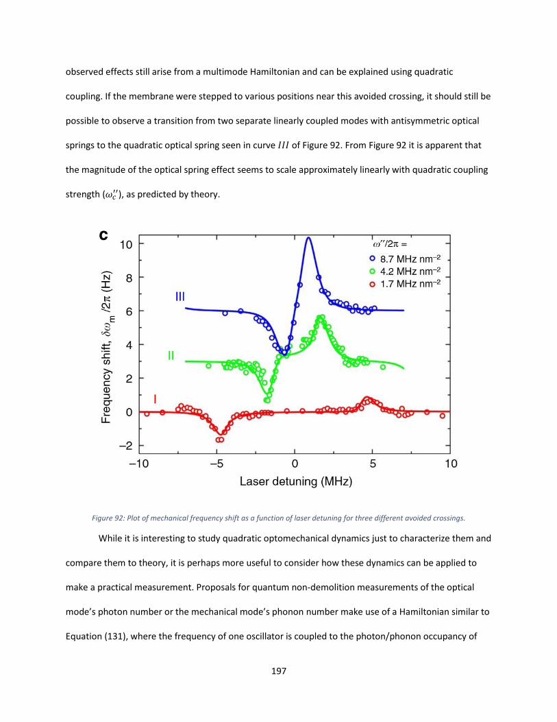
197

observed effects still arise from a multimode Hamiltonian and can be explained using quadratic

coupling. If the membrane were stepped to various positions near this avoided crossing, it should still be

possible to observe a transition from two separate linearly coupled modes with antisymmetric optical

springs to the quadratic optical spring seen in curve 𝐼𝐼𝐼 of Figure 92. From Figure 92 it is apparent that

the magnitude of the optical spring effect seems to scale approximately linearly with quadratic coupling

strength (𝜔𝑐′′), as predicted by theory.

Figure 92: Plot of mechanical frequency shift as a function of laser detuning for three different avoided crossings.

While it is interesting to study quadratic optomechanical dynamics just to characterize them and

compare them to theory, it is perhaps more useful to consider how these dynamics can be applied to

make a practical measurement. Proposals for quantum non-demolition measurements of the optical

mode’s photon number or the mechanical mode’s phonon number make use of a Hamiltonian similar to

Equation (131), where the frequency of one oscillator is coupled to the photon/phonon occupancy of

198

the other. While much stronger quadratic coupling is required to make a measurement that can observe

instantaneous quantum jumps between photon/phonon numbers, 69 weak measurements may still be

able to observe non-classical fluctuations in the photon/phonon number of a driven oscillator. 62, 63 As a

first step in this direction, we used the membrane’s mechanical frequency shift to detect classical

fluctuations of the intracavity photon number.

To perform this demonstration, we used an AOM to modulate the intensity of the control laser

with a modulation depth of 0.77 at 75 Hz. The periodic fluctuations of intracavity power caused by this

modulation result in periodic modulation of the mechanical frequency of the membrane through the

quadratic optical spring effect. In a power spectral density of the motion of the mechanical mode, this

should manifest as 75 Hz frequency modulation sidebands around the membrane’s mechanical

resonance frequency. However, though the depth of the modulation of the control beam is large

enough to produce large variations in intracavity power, the quadratic coupling is quite weak, so these

frequency modulation sidebands are expected to be very small.

For example, the incident laser power used for the curves in Figure 92 was 80 µW. With a cavity

finesse of ℱ ≈ 4,000, this corresponds to a circulating power in the cavity of 𝑃circ = 320 mW. The

intracavity photon number is therefore 𝑛 =𝑃circ

(FSR)(ℏ𝜔𝐿)= 4.3 × 108 photons. Looking at curve 𝐼 in Figure

92, it is clear that these photons produce a frequency shift in the membrane via the quadratic optical

spring effect of about 1.5 Hz. The coupling rate is therefore 3.5 × 10−9Hz photon⁄ , which is quite small.

For a modulation depth of 0.77, the amplitude of the modulation in terms of photon number is

approximately 3.3 × 108 photons, which produces a maximum frequency shift of the mechanical mode

of about 1 Hz. Therefore, though the intensity modulation index of the laser is a large 0.77, the resulting

frequency modulation index (defined as Δ𝑓 𝑓mod⁄ where Δ𝑓 is the maximum frequency deviation and

𝑓mod is the modulation frequency) of the membrane is a tiny 0.013. With such a modulation index, a

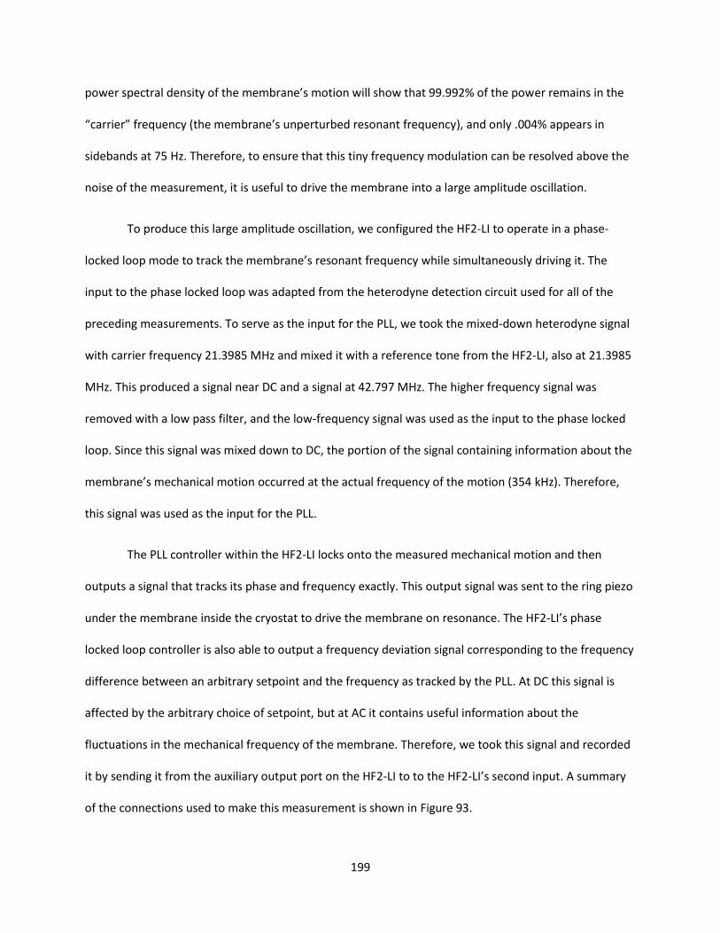
199

power spectral density of the membrane’s motion will show that 99.992% of the power remains in the

“carrier” frequency (the membrane’s unperturbed resonant frequency), and only .004% appears in

sidebands at 75 Hz. Therefore, to ensure that this tiny frequency modulation can be resolved above the

noise of the measurement, it is useful to drive the membrane into a large amplitude oscillation.

To produce this large amplitude oscillation, we configured the HF2-LI to operate in a phase-

locked loop mode to track the membrane’s resonant frequency while simultaneously driving it. The

input to the phase locked loop was adapted from the heterodyne detection circuit used for all of the

preceding measurements. To serve as the input for the PLL, we took the mixed-down heterodyne signal

with carrier frequency 21.3985 MHz and mixed it with a reference tone from the HF2-LI, also at 21.3985

MHz. This produced a signal near DC and a signal at 42.797 MHz. The higher frequency signal was

removed with a low pass filter, and the low-frequency signal was used as the input to the phase locked

loop. Since this signal was mixed down to DC, the portion of the signal containing information about the

membrane’s mechanical motion occurred at the actual frequency of the motion (354 kHz). Therefore,

this signal was used as the input for the PLL.

The PLL controller within the HF2-LI locks onto the measured mechanical motion and then

outputs a signal that tracks its phase and frequency exactly. This output signal was sent to the ring piezo

under the membrane inside the cryostat to drive the membrane on resonance. The HF2-LI’s phase

locked loop controller is also able to output a frequency deviation signal corresponding to the frequency

difference between an arbitrary setpoint and the frequency as tracked by the PLL. At DC this signal is

affected by the arbitrary choice of setpoint, but at AC it contains useful information about the

fluctuations in the mechanical frequency of the membrane. Therefore, we took this signal and recorded

it by sending it from the auxiliary output port on the HF2-LI to to the HF2-LI’s second input. A summary

of the connections used to make this measurement is shown in Figure 93.

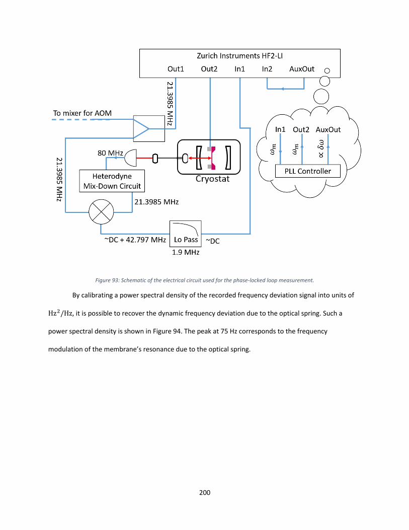
200

Figure 93: Schematic of the electrical circuit used for the phase-locked loop measurement.

By calibrating a power spectral density of the recorded frequency deviation signal into units of

Hz2/Hz, it is possible to recover the dynamic frequency deviation due to the optical spring. Such a

power spectral density is shown in Figure 94. The peak at 75 Hz corresponds to the frequency

modulation of the membrane’s resonance due to the optical spring.

201

Figure 94: Power spectral density of the membrane’s frequency deviation.

Taking the square root of the integral of the 75 Hz peak in Figure 94 gives the RMS frequency

deviation of the of the membrane due to the optical spring. Figure 95 shows plots of this value for

various laser detunings at both a point of quadratic coupling (left) and a point of linear coupling (right).

With quadratic coupling, the maximum frequency deviation occurs when the control laser is directly on

resonance. With linear coupling, the maximum frequency deviation occurs to both sides of resonance.

These results are consistent with the observations of optical spring at quadratic and linear points in

Figure 89a and the theory plots in Figure 76a. The magnitude of the optical spring induced frequency

modulation (~0.2 Hz at a control laser detuning of 0) also roughly agrees with the ballpark prediction

from above. The 1 Hz predicted maximum deviation above corresponds to an RMS deviation of 0.7 Hz,

which matches the observed result within a factor of 3.5.

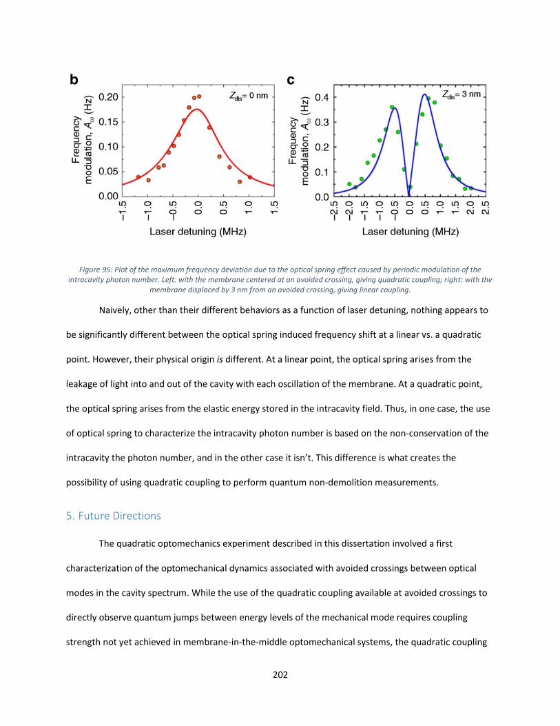
202

Figure 95: Plot of the maximum frequency deviation due to the optical spring effect caused by periodic modulation of the intracavity photon number. Left: with the membrane centered at an avoided crossing, giving quadratic coupling; right: with the

membrane displaced by 3 nm from an avoided crossing, giving linear coupling.

Naively, other than their different behaviors as a function of laser detuning, nothing appears to

be significantly different between the optical spring induced frequency shift at a linear vs. a quadratic

point. However, their physical origin is different. At a linear point, the optical spring arises from the

leakage of light into and out of the cavity with each oscillation of the membrane. At a quadratic point,

the optical spring arises from the elastic energy stored in the intracavity field. Thus, in one case, the use

of optical spring to characterize the intracavity photon number is based on the non-conservation of the

intracavity the photon number, and in the other case it isn’t. This difference is what creates the

possibility of using quadratic coupling to perform quantum non-demolition measurements.

5. Future Directions

The quadratic optomechanics experiment described in this dissertation involved a first

characterization of the optomechanical dynamics associated with avoided crossings between optical

modes in the cavity spectrum. While the use of the quadratic coupling available at avoided crossings to

directly observe quantum jumps between energy levels of the mechanical mode requires coupling

strength not yet achieved in membrane-in-the-middle optomechanical systems, the quadratic coupling

203

at the avoided crossings in our system may be well suited to measurements of phonon shot noise.

Phonon shot noise arises from non-classical fluctuations in the energy level of a mechanical oscillator in

the same way that photon shot noise arises from vacuum fluctuations in an optical field. Careful

measurements of the full counting statistics of such fluctuations in a mechanical oscillator are predicted

to reveal evidence that these fluctuations have a quasiprobability distribution that is not positive-

definite – a sign that these fluctuations cannot be described by any classical theory. 63 Proposals 62 for

measuring phonon shot noise call for a membrane cooled close to its ground state to reduce the

influence of thermal noise on the spectrum of the oscillator’s motion, the ability to drive the membrane

into large amplitude oscillations, and the ability to couple the cavity frequency to the phonon number of

the oscillator. The membrane-in-the-middle system presented in this dissertation is uniquely suited to

this type of measurement because of its ability to simultaneously achieve linear coupling for cooling

using one longitudinal cavity mode and quadratic coupling at an avoided crossing in another longitudinal

cavity mode.

Another step forward from the quadratic optomechanics experiment presented in this

dissertation would be to explore the dynamics of other types of avoided crossings. The experiment

presented here examined only the dynamics of what happens near avoided crossings between the

frequencies of optical cavity modes. Under the right circumstances, such avoided crossings can also be

observed between the frequencies of mechanical modes. Additionally, it is possible to generalize the

concept of avoided crossings by considering eigenvalues in the complex plane, where the imaginary part

of the eigenvalue represents the mode’s damping. When system control parameters are set such that

the complex eigenvalues of two modes become degenerate, there is said to be an exceptional point in

the space of the control parameters. For the mechanical eigenmodes of the membrane-in-the-middle

system, suitable control parameters are laser power and cavity detuning. Theory predicts that the

dependence of the complex eigenvalues upon these parameters has a non-trivial topological structure,

204

which can enable transfer of energy between eigenmodes by way of adiabatic topological operations.

For example, one such operation would be to vary the laser power and detuning in such a way as to

execute a closed loop around an exceptional point in the power-detuning plane. The presence of

different damping rates of the mechanical eigenmodes during this operation is predicted to make the

transfer of energy between modes non-reciprocal. A paper exploring these concepts experimentally was

recently published by the Harris group at Yale using the same membrane-in-the-middle setup described

in the ground state cooling portion of this dissertation. 56

205

V. Conclusion

The field of optomechanics has come a long way since the invention of the photophone.

Modern systems that exploit radiation pressure to interact with macroscopic mechanical oscillators have

demonstrated exceptional sensitivity to small mechanical displacements, and have started to explore

the realm of non-linear coupling between mechanical oscillators and optical cavities. Using

optomechanical systems, ground state cooling of macroscopic oscillators has been demonstrated,

radiation pressure shot noise has been detected, and mechanical quantum states have been prepared.

The future is indeed exciting, as systems begin to demonstrate processes useful for quantum

information processing such as coherent state transfer from the optical field to a mechanical oscillator

and back again.

The work I have described in this dissertation has contributed to the field of optomechanics in

several important ways. First, I have described the cooling of one mechanical mode of a nanogram-scale

silicon nitride membrane to a phonon occupancy of less than one. The large mass and low frequency of

this oscillator compared to many others described in the literature made the cooling of the oscillator

particularly difficult, and required particular attention to the influence of laser noise on the oscillator.

This dissertation therefore describes the many steps we took to minimize the amplitude and phase

noise on our lasers, and to verify that the noise was not significantly affecting the cooling or

measurement of the membrane’s motion. Though the methods used to do this may not in themselves

be novel, the summary presented in this dissertation will most certainly be useful as a reference for

future experiments.

Also in this dissertation, I have described the fundamentals of multimode optomechanics

involving the coupling of one mechanical mode to two (or more) optical modes in the vicinity of avoided

crossings. The results of this experiment demonstrated qualitatively different optomechanical effects

206

than would be expected for coupling to a single optical mode, and the results are consistent with a

simple theory. I have shown that avoided crossings between cavity modes can be locally approximated

as points of quadratic coupling, and described how quadratic coupling can provide access to novel

physical effects such as quantum non-demolition measurements. The demonstration I presented of the

readout of the intracavity photon number by way of the quadratic optical spring effect is a first step

toward such a measurement.

Concluding this dissertation, I hope that I have fairly presented both the history and the state of

the art of the modern field of optomechanics. There are certainly many exciting discoveries to come as

groups across the world push mechanical oscillators further into the quantum regime, and as theory

proposals for optomechanical systems turn into experiments, and then perhaps even into commercial

products. The membrane-in-the-middle system is just one of many systems that will be studied in the

years to come, and it is my hope that this work will be useful in future study.

207

VI. Works Cited

1. Bell, A. G., United States of America Patent No. 235,199 (December 1880).

2. Guillemin, A., El mundo físico: gravedad, gravitación, luz, calor, elctricidad, magnetismo, etc. (Montaner y Simón, Barcelona, 1882).

3. Thompson, S. P., Notes on Construction of the Photophone. Phys. Soc. Pro. 4, 184-190 (1881).

4. Aspelmeyer, M., Kippenberg, T. J. & Marquardt, F., Cavity Optomechanics. arXiv:1303.0733v1 (2013).

5. O'Connell, A. D. et al., Quantum ground state and single-phonon control of a mechanical resonator. Nature 464 (697) (2010).

6. Chan, J. et al., Laser cooling of a nanomechanical oscillator into its quantum ground state. Nature 478, 89-92 (2011).

7. Teufel, J. D. et al., Sideband cooling micromechanical motion to the quantum ground state. Nature 475, 359 (2011).

8. Weinstein, A. J. et al., Observation and Interpretation of Motional Sideband Asymmetry in a Quantum Electromechanical Device. Phys. Rev. X 4 (041003) (2014).

9. Purdy, T. P. et al., Optomechanical Raman-ratio thermometry. Physical Review A 92 (031802(R)) (2015).

10. Mingyun, Y., Singh, V., Blanter, Y. M. & Steele, G. A., Large cooperativity and microkelvin cooling with a three-dimensional optomechanical cavity. Nature Communications 6 (8491) (2015).

11. Underwood, M. et al., Measurement of the motional sidebands of a nanogram-scale oscillator in the quantum regime. Physical Review A 92, 061801(R) (2015).

12. Lecocq, F., Clark, J. B., Simmonds, R. W., Aumentado, J. & Teufel, J. D., Quantum Nondemolition Measurment of a Nonclassical State of a Massive Object. Physical Review X 5 (041037) (2015).

13. Wollman, E. E. et al., Quantum squeezing of motion in a mechanical resonator. Science 349 (6251), 952-955 (2015).

14. Palomaki, T. A., Harlow, J. W., Teufel, J. D., Simmonds, R. W. & Lehnert, K. W., Coherent state transfer between itinerant microwave fields and a mechanical oscillator. Nature 495, 210-214 (2013).

15. Andrews, R. W. et al., Bidirectional and effficient conversion between microwave and optical light. Nature Physics 10, 321 (2014).

208

16. McGee, S. A., Meiser, D., Regal, C. A., Lehnert, K. W. & Holland, M. J., Mechanical resonators for storage and transfer of electrical and optical quantum states. Physical Review A 87 (053818) (2013).

17. Einstein, A., Zum gegenwärtigen Stand des Strahlungsproblems. Physikalische Zeitschrift 10, 185-193 (1909).

18. Braginsky, V. B. & Khalili, F. Y., Quantum Measurement (Cambridge University Press, 1995).

19. Caves, C. M., Quantum-mechanical radiation-pressure fluctuations in an interferometer. Phys. Rev. Lett. 45 (75) (1980).

20. Marquardt, F., Chen, J. P., Clerk, A. A. & Girvin, S. M., Quantum Theory of Cavity Assisted Sideband Cooling of Mechanical Motion. Physical Review Letters 99, 093902 (2007).

21. Khalili, F. Y. et al., Quantum back-action in measurements of zero-point mechanical oscillations. Physical Review A 86 (033840) (2012).

22. Purdy, T. P., Peterson, R. W. & Regal, C. A., Observation of Radiation Pressure Shot Noise on a Macroscopic Object. Science 339 (801-804) (2013).

23. Clerk, A. A., Marquardt, F. & Jacobs, K., Back-action evasion and squeezing of a mechanical resonator using a cavity detector. New Journal of Physics 10 (095010) (2008).

24. Abbot, B. P., et al., Observation of Gravitational Waves from a Binary Black Hole Merger. Physical Review Letters 116 (061102) (2016).

25. Purdy, T., Yu, P.-L., Peterson, R. W., Kampel, N. S. & Regal, C. A., Strong Optomechanical Squeezing of Light. Physical Review X 3 (031012) (2013).

26. Braginskiĭ, V. B., Manukin, A. B. & Tikhonov, M. Y., Investigation of Dissipative Ponderomotive Effects of Electromagnetic Radiation. Soviet Physics JETP 31 (5) (1970).

27. Wilson-Rae, I., Nooshi, N., Zwerger, W. & Kippenberg, T. J., Theory of Ground State Cooling of a Mechanical Oscillator Using Dynamical Backaction. Physical Review Letters 99, 093901 (2007).

28. Safavi-Naeini, A. H. et al., Observation of quantum motion of a nanomechanical resonator. Phys. Rev. Lett. 108 (033602) (2012).

29. Meenehan, S. M., Cohen, J. D., MacCabe, G. S. . M. F., Shaw, M. D. & Painter, O., Pulsed Excitation Dymanics of an Optomechanical Crystal Resonator near Its Quantum Ground State of Motion. Physical Review X 5 (041002) (2015).

30. Safavi-Naeini, A. H. et al., Squeezed light from a silicon micromechanical resonator. Nature 500, 185-189 (2013).

31. Paraïso, T. K. et al., Position-squared coupling in a tunable photonic crystal optomechanical cavity. Physical Review X 5 (041024) (2015).

32. Palomaki, T. A., Teufel, J. D., Simmonds, R. W. & Lehnert, K. W., Entangling Mechanical Motion with Microwave Fields. Science 342, 710-713 (2013).

209

33. Lecocq, F., Teufel, J. D., Aumentado, J. & Simmonds, R. W., Resolving the vacuum fluctuations of an optomechanical system using an artificial atom. Nature Physics (Advance Online Publication) (2015).

34. Hertzberg, J. B. et al., Back-action-evading measurements of nanomechanical motion. Nature Physics 6, 213-217 (2010).

35. Suh, J. et al., Mechanically Detecting and Avoiding the Quantum Fluctuations of the Microwave Field. Science 344 (6189), 1262-1265 (2014).

36. Thompson, J., Senior Essay (Yale), 2007.

37. Thompson, J. D. et al., Strong dispersive coupling of a high-finesse cavity to a micromechanical membrane. Nature 452 (72) (2008).

38. Black, E., An introduction to Pound-Drever-Hall laser frequency stabilization. American Journal of Physics 69 (1) (2001).

39. Zwickl, B. M., PhD Thesis (Yale), 2011.

40. Børkje, K. et al., Observability of radiation-pressure shot noise in optomechanical systems. Physical Review A 82 (013818) (2010).

41. Yang, C., PhD Thesis (Yale), 2011.

42. Jayich, A., PhD Thesis (Yale), 2011.

43. Sankey, J. C., Yang, C., Zwickl, B. M., Jayich, A. M. & Harris, J. G. E., Strong and tunable nonlinear optomechanical coupling in a low-loss system. Nature Physics 6, 707-712 (2010).

44. Lee, D. et al., Multimode optomechanical dynamics in a cavity with avoided crossings. Nature Communications 6 (6232) (2015).

45. Griffiths, D. J., Introduction to Electrodynamics (Prentice Hall, Inc., Upper Saddle River, NJ, 1999).

46. Jayich, A. M. et al., Dispersive optomechanics: A membrane inside a cavity. New Journal of Physics 10 (095008) (2008).

47. Brooker, G., Modern Classical Optics (Oxford University Press, Oxford, 2003).

48. Müller, T., Reinhardt, C. & Sankey, J. C., Enhanced optomechanical levitation of minimally supported dielectrics. Physical Review A 91, 053849 (2015).

49. Sankey, J. C., Jayich, A. M., Zwickl, B. M., Yang, C. & Harris, J. G. E., Improved "Position Squared" Readout Using Degenerate Cavity Modes, presented at ICAP, 2008 (unpublished).

50. Marquardt, F., Quantum Optomechanics, presented at Les Houches 2011, Quantum Machines: Measurment and Control of Engineered Quantum Systems, New York, 2011 (unpublished).

210

51. Jayich, A. M. et al., Cryogenic optomechanics with a Si3N4 membrane and classical laser noise. New J. Phys. 14 (115018) (2012).

52. Norcada, High-Q Si3N4 Membrane Windows, Available at http://www.norcada.com/products/high-q-si3n4-membrane/.

53. Pobell, F., Matter and Methods at Low Temperatures, 2nd ed. (Springer-Verlag, Berlin, 1996).

54. Zwickl, B. M. et al., High quality mechanical and optical properties of commercial silicon nitride membranes. Applied Physics Letters 92 (103125) (2008).

55. Schünemann, U., Engler, H., Grimm, R., Weidemüller, M. & Zielonkowski, M., Simple sheme for tunable frequency offset locking of two lasers. Review of Scientific Instruments 70 (1) (1999).

56. Xu, H., Mason, D., Jiang, L. & Harris, J. G. E., Topological energy transfer in an optomechanical system with exceptional points. arXiv:1602.06881 (2016).

57. Wanser, K. H., Fundamental Phase Noise Limit in Optical Fibres Due to Temperature Fluctuations. Electronics Letters 28 (1) (1992).

58. Bartolo, R. E., Tveten, A. B. & Dandridge, A., Thermal Phase Noise Measurements in Optical Fiber Interferometers. IEEE Journal of Quantum Electronics 48 (5) (2012).

59. Yuan, M., Cohen, M. A. & Steele, G. A., Silicon nitride membrane resonators at millikelvin temperatures with quality factors exceeding 10^8. Applied Physics Letters 107, 263501 (2015).

60. Yu, P.-L. et al., A phononic bandgap shield for high-Q membrane microresonators. Applied Physics Letters 104 (023510) (2014).

61. Asjad, M. et al., Robust stationary mechanical squeezing in a kicked quadratic optomechanical system. Physical Review A 98 (023849) (2014).

62. Clerk, A. A., Marquardt, F. & Harris, J. G. E., Quantum Measurement of Phonon Shot Noise. Physical Review Letters 104, 213603 (2010).

63. Clerk, A. A., Full counting statistics of energy fluctuations in a driven quantum resonator. Physical Review A 84, 043824 (2011).

64. Flowers-Jacobs, N. E. et al., Fiber-cavity-based optomechanical device. Applied Physics Letters 101 (221109) (2012).

65. Karuza, M. et al., Tunable linear and quadratic optomechanical coupling for a tilted membrane within an optical cavity: theory and experiment. Journal of Optics 15 (025704) (2013).

66. Purdy, T. P. et al., Tunable Cavity Optomechanics with Ultracold Atoms. Physical Review Letters 105 (133602) (2010).

67. Hill, J. T., Lin, Q., Rosenberg, J. & Painter, O., Mechanical Trapping in a Quadratically-Coupled Optomechanical Double Disk, presented at IEEE Conference on Lasers and Electro-Optics, 2011 (unpublished).

211

68. Hill, J. T., PhD Thesis (Caltech), 2013.

69. Miao, H., Danilishin, S., Corbitt, T. & Chen, Y., Standard Quantum Limit for Probing Mechanical Energy Quantization. Physical Review Letters 103 (100402) (2009).