Aalborg Universitet Auditory temporal resolution and...

Aalborg Universitet

Auditory temporal resolution and integration - stages of analyzing time-varying sounds

Pedersen, Benjamin

Publication date:2007

Document VersionPublisher's PDF, also known as Version of record

Link to publication from Aalborg University

Citation for published version (APA):Pedersen, B. (2007). Auditory temporal resolution and integration - stages of analyzing time-varying sounds.Aalborg University.

General rightsCopyright and moral rights for the publications made accessible in the public portal are retained by the authors and/or other copyright ownersand it is a condition of accessing publications that users recognise and abide by the legal requirements associated with these rights.

? Users may download and print one copy of any publication from the public portal for the purpose of private study or research. ? You may not further distribute the material or use it for any profit-making activity or commercial gain ? You may freely distribute the URL identifying the publication in the public portal ?

Take down policyIf you believe that this document breaches copyright please contact us at [email protected] providing details, and we will remove access tothe work immediately and investigate your claim.

Downloaded from vbn.aau.dk on: juni 22, 2018

http://vbn.aau.dk/en/publications/auditory-temporal-resolution-and-integration--stages-of-analyzing-timevarying-sounds(f0799550-3b73-11dc-b148-000ea68e967b).html

Auditory Temporal Resolution and Integration

Stages of Analyzing Time-Varying Sounds

PhD thesis

by

Benjamin Pedersen

September 2006

Sound Quality Research Unit

Department of Acoustics

Aalborg University

Preface

This thesis has been submitted to the Faculty of Engineering, Science and Medicine at Aalborg Uni-versity for partial fulfillment of the requirements for the award of the PhD degree. The research wascarried out at the Sound Quality Research Unit at the university’s Department of Acoustics in the periodfrom September 2002 to October 2006.

I would like to thank all people of the Sound Quality Research Unit for mutual and fruitful ex-change of ideas. I would also like to thank people of the Department of Acoustic who contributed withtechnical assistance or valuable feedback. Part of this research was carried out at the PsychoacousticsLaboratory (directed by Neal Viemeister) at the Department of Psychology, University of Minnesota,USA. I would like to thank the people of the laboratory for their hospitality and scientific feedbackduring the research visit.

The work of the Sound Quality Research Unit was partially funded by the companies Brüel &Kjær, DELTA Acoustics & Vibration, and Bang & Olufsen. Further financial support came from theMinistry for Science, Technology, and Development (VTU), and from the Danish Research Councilfor Technology and Production (FTP).

Especially I would like to thank Wolfgang Ellermeier for his supervision during the entire PhDproject. His influence has positively and significantly shaped the outcome of the project and the devel-opment of my professional skills.

Finally, I would also like to thank the members of the PhD assessment committee for constructiveremarks and suggestion concerning the content of this thesis.

Benjamin PedersenAalborg, September 2006

The paper presented in Chapter 2 was published in a revised version in the Journal of the AcousticalSociety of America after the publication of the thesis:

Pedersen, B. and Ellermeier, W. (2008). “Temporal weights in the level discrimination of time-varyingsounds.”, J. Acoust. Soc. Am. 123, 963–972.

i

Summary

An important property of sound is its variation as a function of time, which carries much relevantinformation about the origin of a given sound. Further, in analyzing the “meaning” of a sound per-ceptually, the temporal variation is of tremendous importance. In spite of its perceptual importance,much is still unknown of how temporal information is analyzed and represented in the auditory sys-tem. Specifically, a large body of research has been concerned with identifying the acuity with whichthe temporal information is represented in the sensory system, and this has lead to some seeminglyparadoxal observations: In binaural experiments (different sounds at the two ears) listeners are able torely on temporal cues in the difference between the input from the two ears with a very fine resolution(∼ 10 µs), whereas, when the same stimulation is provided to both ears, the listeners’ ability to relyon temporal cues is much worse (∼ 3 ms). For temporal integration of sound at levels close to thethreshold of hearing, critical time-coefficients for integration seem to be as long as 100 ms to 200 ms.Furthermore, the temporal “acuity” also varies greatly over auditory tasks of different nature (temporalmasking, gap detection, stream segregation, amplitude modulation detection, temporal order detection,etc.). The listening experiments presented in this thesis are all related to temporal resolution and inte-gration in diotic listening (same sound to both ears). The purpose of the experiments is to clarify someof the apparent discrepancies by probing the auditory system in tasks of different “nature” in an effortto identify how different stages of perception might be responsible for the performance in the differenttasks.

Specifically, the auditory tasks of the experiments in this thesis may be considered as falling intotwo categories: (1) Temporal integration when listeners have to judge the overall loudness of relativelylong (compared to the temporal resolution of the auditory system) sounds fluctuating in level, and (2)temporal pattern recognition where listeners have to identify properties of the actual patterns of levelchanges.

In two experiments (falling into the first category) listeners had to judge sounds, with a durationof one second and randomly varying in level, as being either “loud” or “soft”. From these judgments,temporal weighting curves were derived and showed that listeners generally emphasized onsets andoffsets of the sounds in their judgments, but in idiosyncratic ways. Additionally, the temporal weight-ing changed if listeners were provided with feedback. In the second experiment, a spectral change wasintroduced in the center of sounds, leading to a perceptual emphasis of the temporal location of thespectral change in loudness judgments. These observations lead to the conclusion that loudness inte-gration is not adequately described by a simple “summation” procedure as assumed in several modelsof loudness integration, but rather, auditory attention seem to be an important aspect when interpretingthe results.

In two further experiments (falling into the second category) listeners had to discriminate temporalpatterns in the envelope of noise samples being either ascending or descending in level. The durationof these patterns was varied to identify the temporal limit where discrimination was no longer possible.The limit was found to be in the order of 1 ms. The task was varied by adding flanking noise on bothsides of the pattern to be identified, which dramatically changed the limit for the discrimination (toapproximately 30 ms). The analysis of the results suggests that a key to understand this differencemight be that, without the flanking noise, the patterns can be discriminated based on onset/offset cues,

iii

which are absent in the case of flanking noise being present. Thus, the underlying hypothesis suggeststhat especially onsets of sounds have a particular elaborate representation in the sensory system. In twofurther conditions, examining the sensory processing of temporal variation, the pattern to be discrim-inated was repeated several times within a fixed time-frame (0.75 s). In the two conditions either theenvelope only or the temporal fine-structure of the patterns was repeated. For relatively long durationsof the patterns, the performance of the listeners was very similar in the two conditions, but for relativelyshort durations of the patterns the performance of the listeners seemed to be fundamentally differentin the two conditions. When repeating the envelope only, listeners’ performance was very similar tothe case where the pattern was not repeated, but when the fine-structure was repeated, listeners wereable to discriminate patterns with a much finer resolution. In the case of repeated fine-structure, noabsolute lower temporal limit was found even though the duration of a single patterns was as short as60 µs. Further, in the condition where the fine-structure was repeated, adding flanking noise seemedto improve rather than impair performance of the listeners for the shortest durations of the patterns.This shows that the concept of “energetic masking”, which is often used to explain the performanceof listeners, may be inadequate as it predicts that adding noise should worsen performance. Further, itmight be noted that a temporal resolution of 60 µs is far better than what is normally considered thetemporal limit of the auditory sensory system in the case of diotic stimulation.

The effects observed in the experiments presented in this thesis are too diverse to be adequatelydescribed by a single stage responsible for temporal processing. Therefore, in the thesis, several stagesare suggested and an attempt is made to identify properties of their critical operating range. This par-tially explains the diversity of the measures of temporal resolution obtained in research concerned withauditory temporal processing, but much is still left to be explained. Hopefully the research presentedin this thesis will help in disentangling different effects observed in listening experiments concernedwith temporal processing.

iv

Resumé (Summary in Danish)

En vigtig egenskab ved lyd er dens variation som en funktion af tid, hvilken indeholder vigtig informa-tion om lydens oprindelse. Yderligere er den tidsafhængige varians af største vigtighed for perceptuelanalyse af lydens “mening”. Trods den afgørende betydning for perception er meget stadig uvist om,hvordan lyd repræsenteres og analyseres tidsmæssigt i det auditive system. Meget forskning har be-skæftiget sig med at identificere med hvilken opløsning tidsvarians er repræsenteret i det sensoriskesystem, hvilket har ledt til en række tilsyneladende paradokser: I binaurale forsøg (forskellig lyd vedde to ører) er forsøgspersoner i stand til at detektere meget små tidsmæssige forskelle (∼ 10 µs). Der-imod er de slet ikke i stand til at detektere tidsvarians med en sådan opløsning, når det samme inputgives til begge ører (∼ 3 ms tidsmæssige forskelle kan detekteres). For integration af lyde med niveau-er tæt ved høretærsklen er der tegn på, at tidsperioden for integration er så lang som 100 ms til 200ms. Den tidsmæssige opløsning varierer også stærkt ved opgaver stillet i forskellige typer lytteforsøg(forsøgskategorier på engelsk: Temporal masking, gap detection, stream segregation, amplitude modu-lation detection, temporal order detection, etc.). Lytteforsøgene, der præsenteres i denne afhandling,relaterer alle til tidsmæssig opløsning (temporal resolution) og integration i diotisk hørelse (sammeinput til begge ører). Formålet med forsøgene er at afklare nogle af disse tilsyneladende uoverensstem-melser ved at teste det auditive system i opgaver af forskellig “natur”. Dette hjælper til at identificere,hvorledes forskellige perceptuelle niveauer er involveret, når forsøgspersonerne løser opgaver i for-skellige typer forsøg.

Forsøgene, som beskrives i denne afhandling, kan betragtes som faldende i to kategorier: (1) Tids-mæssig integration når forsøgspersoner skal bedømme den samlede lydstyrke (loudness) af relativtlange lyde (i sammenligning med det auditive systems evne til at detektere tidsmæssig varians), somfluktuerer i lydstyrke, og (2) genkendelse af mønstre, hvor forsøgspersoner skal identificere mønstrebestemt ved deres variation i lydstyrke som funktion af tid.

I to forsøg (som falder i den første kategori) skulle forsøgspersoner bedømme lyde af et sekunds va-righed og tilfældigt varierende i lydstyrke, som værende enten “høje” eller “lave”. På grundlag af dissebedømmelser, blev tidsmæssige vægtningskurver beregnet, og de viste at forsøgspersonerne i deressvar generelt lagde ekstra vægt på en lyds begyndelse og slutning, men på meget individuelle måder.Yderligere ændredes vægtningen når forsøgspersonerne fik feedback. Et skift i lydens spektrum i mid-ten af en lyd blev introduceret i en ny forsøgsbetingelse, hvilket førte til at forsøgspersonerne ogsålagde ekstra vægt på skiftet i spektrum. Disse observationer (samt andre) fører til den konklusion, atintegration af lydstyrke (loudness integration) ikke passende kan beskrives som en simpel summerings-proces, som det antages i flere modeller for integration af lydstyrke, men snarere synes et begreb somauditiv opmærksomhed at være vigtig for at forstå resultaterne.

I yderligere to forsøg (faldende i den anden kategori) skulle forsøgspersoner skelne tidsmæssigemønstre i et støjsignals lydniveau som værende enten opad- eller nedadgående. Den tidsmæssige ud-strækning af sådanne mønstre blev varieret for at finde den tidsmæssige grænse for, hvor mønstrenekunne skelnes. Grænsen var cirka ved 1 ms. Opgaven blev varieret ved at tilføje ikke-informativ støj påbegge sider af mønstret, som skulle genkendes. Dette ændrede den tidsmæssige grænse kraftigt (nu ca.30 ms). Analyse af resultaterne antyder, at nøglen til at forstå denne forskel ligger i, at uden den ikke-informative støj kan mønstrene skelnes på grundlag af deres forskelighed ved start og slut (onset/offset

v

cues). Dette er ikke muligt i det tilfælde, hvor støj er tilstede ved lydens start og slutning. Den grund-liggende hypotese er, at specielt lyds begyndelse har en detaljeret repræsentation i sansesystemet. I toyderligere forsøgsbetingelser, der undersøger den sensoriske behandling af tidsmæssig variation, blevmønstrene, som skulle skelnes, gentaget flere gange indenfor et bestemt tidsinterval (0.75 s). I de to for-søgsbetingelser blev et enkelt mønster gentaget enten i detaljeret grad (fine-structure), eller også blevkun omridset (envelope) af et mønster gentaget. For relativt lang varighed af et mønster var forsøgsper-sonernes evne til at skelne mønstre næsten ens i de to betingelser, men for relativt korte mønstre var derstor forskel. Når kun omridset blev gentaget, var der næsten ingen forskel i forsøgspersonernes ydelsefra det tilfælde, hvor der ingen gentagelse var. Hvis derimod mønstret blev gentaget i detaljeret grad,var personerne i stand til at skelne mønstrene i meget finere grad. I tilfældet hvor mønstret blev gentageti detaljeret grad blev der ikke fundet nogen nedre grænse for, hvornår mønstrene kunne skelnes, selvomudstrækningen af et enkelt mønster var så lav som 60 µs. Når mønstret blev gentaget i detaljeret grad,syntes tilføjelsen af ikke-informativ støj snarere at forbedre end at forringe forsøgspersonernes ydelseved kort mønstervarighed. Dette viser at begrebet “energimæssig maskering” (energetic masking), somnormalt bruges til at forklare forsøgspersoners ydelse, kan være fundamentalt forkert, da det forudsiger,at tilføjelsen af støj generelt skulle forværre forsøgspersonernes ydelse. Til sidst kan det bemærkes, atden observerede tidsopløsning på 60 µs er langt finere, end hvad der normalt betragtes som den nedregrænse for det auditive sensoriske system ved diotisk stimulation (samme input til begge ører).

Observationerne for tidsmæssig integration præsenteret i denne afhandling er så forskelligartede,at de vanskeligt kan beskrives med en enkelt enhed, som er ansvarlig for den tidsmæssige behandling.Derfor bliver det forslået at flere enheder er aktive, og egenskaber ved enhedernes virkeområde forsøgesafgrænset. Dette er i en hvis grad i stand til at forklare forskelligartetheden af de mål, der i forskninger opnået for tidsintegration, men meget er stadig tilbage at forstå. Forhåbentlig vil resultaterne, somer fremlagt i denne afhandling, hjælpe til at adskille og forstå observationer opnået i lytteforsøg, derbeskæftiger sig med tidsintegration i hørelsen.

vi

Contents

Preface i

Summary iii

Resumé (Summary in Danish) v

1 Introduction 11.1 Frequency and temporal analysis . . . . . . . . . . . . . . . . . . . . . . . . . . . . . 21.2 Probing the hearing system’s capabilities in temporal analysis . . . . . . . . . . . . . . 21.3 Diverging measures of temporal resolution . . . . . . . . . . . . . . . . . . . . . . . . 31.4 Goals and arrangement of the thesis . . . . . . . . . . . . . . . . . . . . . . . . . . . 31.5 General results . . . . . . . . . . . . . . . . . . . . . . . . . . . . . . . . . . . . . . 4

1.5.1 Results and conclusions of Chapter 2 . . . . . . . . . . . . . . . . . . . . . . 41.5.2 Results and conclusions of Chapter 3 . . . . . . . . . . . . . . . . . . . . . . 41.5.3 Results and conclusions of Chapter 4 . . . . . . . . . . . . . . . . . . . . . . 51.5.4 Results and conclusions of Chapter 5 . . . . . . . . . . . . . . . . . . . . . . 6

1.6 General conclusions . . . . . . . . . . . . . . . . . . . . . . . . . . . . . . . . . . . . 7

2 Paper 1:Temporal weighting in loudness judgments of level-fluctuating sounds 11I Introduction . . . . . . . . . . . . . . . . . . . . . . . . . . . . . . . . . . . . . . . . 13

I.A Weighting level information in auditory discrimination tasks . . . . . . . . . . 13I.B Memory effects . . . . . . . . . . . . . . . . . . . . . . . . . . . . . . . . . . 14I.C Rationale . . . . . . . . . . . . . . . . . . . . . . . . . . . . . . . . . . . . . 14

II Experiment 1 - Loudness of single sounds . . . . . . . . . . . . . . . . . . . . . . . . 14II.A Method . . . . . . . . . . . . . . . . . . . . . . . . . . . . . . . . . . . . . . 14II.B Results of Experiment 1 . . . . . . . . . . . . . . . . . . . . . . . . . . . . . 16II.C Discussion . . . . . . . . . . . . . . . . . . . . . . . . . . . . . . . . . . . . 17

III Experiment 2 - Loudness of two-event sounds . . . . . . . . . . . . . . . . . . . . . . 17III.A Introduction . . . . . . . . . . . . . . . . . . . . . . . . . . . . . . . . . . . . 17III.B Method . . . . . . . . . . . . . . . . . . . . . . . . . . . . . . . . . . . . . . 17III.C Results of Experiment 2 . . . . . . . . . . . . . . . . . . . . . . . . . . . . . 20III.D Discussion . . . . . . . . . . . . . . . . . . . . . . . . . . . . . . . . . . . . 20

IV Final discussion and conclusion . . . . . . . . . . . . . . . . . . . . . . . . . . . . . 22V Acknowledgments . . . . . . . . . . . . . . . . . . . . . . . . . . . . . . . . . . . . 23

3 Modeling level discrimination:Non-linear and across-trial effects 253.1 Introduction . . . . . . . . . . . . . . . . . . . . . . . . . . . . . . . . . . . . . . . . 253.2 Effects across trials . . . . . . . . . . . . . . . . . . . . . . . . . . . . . . . . . . . . 26

vii

3.2.1 Level-independent effects . . . . . . . . . . . . . . . . . . . . . . . . . . . . 263.2.2 Level dependent effects across trials . . . . . . . . . . . . . . . . . . . . . . . 283.2.3 Changes in weighing curve as a function of time . . . . . . . . . . . . . . . . 30

3.3 Modeling the decision process . . . . . . . . . . . . . . . . . . . . . . . . . . . . . . 303.3.1 Model-independent observations . . . . . . . . . . . . . . . . . . . . . . . . . 30

3.4 Applying a temporal loudness model . . . . . . . . . . . . . . . . . . . . . . . . . . . 353.4.1 Evaluating models of time-varying loudness . . . . . . . . . . . . . . . . . . . 363.4.2 Temporal window . . . . . . . . . . . . . . . . . . . . . . . . . . . . . . . . 41

3.5 Alternative models of loudness judgments . . . . . . . . . . . . . . . . . . . . . . . . 423.5.1 Fitting procedure . . . . . . . . . . . . . . . . . . . . . . . . . . . . . . . . . 423.5.2 Assessing model fits . . . . . . . . . . . . . . . . . . . . . . . . . . . . . . . 453.5.3 The “best” model . . . . . . . . . . . . . . . . . . . . . . . . . . . . . . . . . 51

3.6 Response time and loudness . . . . . . . . . . . . . . . . . . . . . . . . . . . . . . . 533.6.1 Data collection . . . . . . . . . . . . . . . . . . . . . . . . . . . . . . . . . . 543.6.2 Response time results . . . . . . . . . . . . . . . . . . . . . . . . . . . . . . . 543.6.3 Discussion . . . . . . . . . . . . . . . . . . . . . . . . . . . . . . . . . . . . 56

3.7 Temporal weights in a comparison task . . . . . . . . . . . . . . . . . . . . . . . . . . 593.7.1 Data collection . . . . . . . . . . . . . . . . . . . . . . . . . . . . . . . . . . 593.7.2 Results . . . . . . . . . . . . . . . . . . . . . . . . . . . . . . . . . . . . . . 593.7.3 Stimuli of 200 ms duration . . . . . . . . . . . . . . . . . . . . . . . . . . . . 613.7.4 Summary . . . . . . . . . . . . . . . . . . . . . . . . . . . . . . . . . . . . . 61

3.8 Conclusions . . . . . . . . . . . . . . . . . . . . . . . . . . . . . . . . . . . . . . . . 623.8.1 Temporal loudness integration is not a simple summation process . . . . . . . 623.8.2 Temporal loudness integration is a non-linear process . . . . . . . . . . . . . . 63

4 Paper 2:Temporal masking in the auditory identification of envelope patterns 65I Introduction . . . . . . . . . . . . . . . . . . . . . . . . . . . . . . . . . . . . . . . . 67

I.A Stages in modeling hearing . . . . . . . . . . . . . . . . . . . . . . . . . . . . 67I.B Neurophysiological and psychoacoustical evidence for different stages in hearing 68I.C Probing “low” or “high” cognitive stages in listening experiments? . . . . . . . 68I.D A task probing several levels of perception . . . . . . . . . . . . . . . . . . . 69

II Method . . . . . . . . . . . . . . . . . . . . . . . . . . . . . . . . . . . . . . . . . . 69II.A Listeners . . . . . . . . . . . . . . . . . . . . . . . . . . . . . . . . . . . . . 69II.B Apparatus . . . . . . . . . . . . . . . . . . . . . . . . . . . . . . . . . . . . . 69II.C Stimuli . . . . . . . . . . . . . . . . . . . . . . . . . . . . . . . . . . . . . . 69II.D Experimental procedure . . . . . . . . . . . . . . . . . . . . . . . . . . . . . 71II.E Data collection . . . . . . . . . . . . . . . . . . . . . . . . . . . . . . . . . . 71

III Results . . . . . . . . . . . . . . . . . . . . . . . . . . . . . . . . . . . . . . . . . . . 71III.A Procedure for deriving psychometric functions . . . . . . . . . . . . . . . . . 71III.B Procedure for estimating performance level . . . . . . . . . . . . . . . . . . . 71III.C Temporal limits for individual listeners . . . . . . . . . . . . . . . . . . . . . 72III.D Individual psychometric functions . . . . . . . . . . . . . . . . . . . . . . . . 72III.E Comparing 3- with 5-segment condition and 9- with 21-segment condition . . 73

IV Discussion . . . . . . . . . . . . . . . . . . . . . . . . . . . . . . . . . . . . . . . . . 73IV.A Predictions of a temporal window model . . . . . . . . . . . . . . . . . . . . 74IV.B Comparison to temporal order judgments of tones . . . . . . . . . . . . . . . . 75IV.C Quality cues and temporal representation . . . . . . . . . . . . . . . . . . . . 75

V Conclusion . . . . . . . . . . . . . . . . . . . . . . . . . . . . . . . . . . . . . . . . 75

viii

Contents ix

V.A Temporal masking and gap detection . . . . . . . . . . . . . . . . . . . . . . 76VI Acknowledgments . . . . . . . . . . . . . . . . . . . . . . . . . . . . . . . . . . . . 76A Quantization of segment durations . . . . . . . . . . . . . . . . . . . . . . . . . . . . 76B Spectrum of noise carrier . . . . . . . . . . . . . . . . . . . . . . . . . . . . . . . . . 77C Sound level at ear . . . . . . . . . . . . . . . . . . . . . . . . . . . . . . . . . . . . . 78D Examples of output of sliding window . . . . . . . . . . . . . . . . . . . . . . . . . . 78E Identical difference between ascending and descending patterns across 3-, 5-, 9-, and

21-segment conditions . . . . . . . . . . . . . . . . . . . . . . . . . . . . . . . . . . 78

5 Paper 3:Discrimination of temporal patterns on the basis of envelope and fine-structure cues 83I Introduction . . . . . . . . . . . . . . . . . . . . . . . . . . . . . . . . . . . . . . . . 85

I.A Repeating pattern - importance of envelope and fine-structure . . . . . . . . . 85I.B Static features . . . . . . . . . . . . . . . . . . . . . . . . . . . . . . . . . . . 85I.C Temporal processing in pitch and timbre perception . . . . . . . . . . . . . . . 86

II Method . . . . . . . . . . . . . . . . . . . . . . . . . . . . . . . . . . . . . . . . . . 86II.A Listeners . . . . . . . . . . . . . . . . . . . . . . . . . . . . . . . . . . . . . 86II.B Apparatus . . . . . . . . . . . . . . . . . . . . . . . . . . . . . . . . . . . . . 86II.C Stimuli . . . . . . . . . . . . . . . . . . . . . . . . . . . . . . . . . . . . . . 86II.D Experimental procedure . . . . . . . . . . . . . . . . . . . . . . . . . . . . . 87II.E Data collection . . . . . . . . . . . . . . . . . . . . . . . . . . . . . . . . . . 89

III Results . . . . . . . . . . . . . . . . . . . . . . . . . . . . . . . . . . . . . . . . . . . 89III.A Procedure for deriving psychometric functions . . . . . . . . . . . . . . . . . 89III.B Procedure for estimating performance level . . . . . . . . . . . . . . . . . . . 89III.C Results of the first phase . . . . . . . . . . . . . . . . . . . . . . . . . . . . . 90III.D Results of the second phase . . . . . . . . . . . . . . . . . . . . . . . . . . . 90

IV Discussion . . . . . . . . . . . . . . . . . . . . . . . . . . . . . . . . . . . . . . . . . 92IV.A Sensory stages of processing temporal information . . . . . . . . . . . . . . . 92IV.B Temporal masking and modeling . . . . . . . . . . . . . . . . . . . . . . . . . 93IV.C Monaural and binaural phase sensitivity . . . . . . . . . . . . . . . . . . . . . 94

V Conclusion . . . . . . . . . . . . . . . . . . . . . . . . . . . . . . . . . . . . . . . . 95V.A Topics for further inquiry . . . . . . . . . . . . . . . . . . . . . . . . . . . . . 95

VI Acknowledgments . . . . . . . . . . . . . . . . . . . . . . . . . . . . . . . . . . . . 95A Quantization of segment durations . . . . . . . . . . . . . . . . . . . . . . . . . . . . 95B Spectrum of noise carrier . . . . . . . . . . . . . . . . . . . . . . . . . . . . . . . . . 95

Appendices 97

A Loudness models: Specifications and evaluations 97A.1 Specification of models for prediction of loudness judgments . . . . . . . . . . . . . . 97A.2 Non-linearity in model predictions . . . . . . . . . . . . . . . . . . . . . . . . . . . . 107

B Spectra of repeating patterns 109B.1 Spectrum of repeating stimuli . . . . . . . . . . . . . . . . . . . . . . . . . . . . . . . 109

B.1.1 Procedure for recording . . . . . . . . . . . . . . . . . . . . . . . . . . . . . 109B.1.2 Impulse response of headphones . . . . . . . . . . . . . . . . . . . . . . . . . 109B.1.3 Computing the amplitude spectrum . . . . . . . . . . . . . . . . . . . . . . . 110

Bibliography 131

Chapter 1

Introduction

Hearing is crucial for humans in that it enables them to communicate and react to their environment.Ultimately the life of an individual depends on whether he or she is able to analyze the surroundings andmake the right actions. Further, communication is paramount for the development of social relationsand for development of the individual’s understanding of the world.

Hearing has the exquisite task of transforming sound, which in itself merely consists of vibrationsof air molecules, into something meaningful. This requires extensive processing, and the full com-plexity of the working of the auditory sensory system is far from understood. Such knowledge isrequired, however, to be able to help people with hearing deficits, or in understanding how sounds ofthe environment (noise for example) influence humans, or in designing high-quality systems for soundreproduction or recording.

It is helpful to always have the basic purposes of hearing in mind, when trying to understand itsfunctioning. In a first step toward a better understanding it may be beneficial to realize that the auditorysensory system must solve several tasks of different nature: (1) The ear has to act as a “microphone”transforming the acoustic vibration into neural electric/chemical activity, and (2) decode (identify prop-erties and features) and (3) convey (from periphery to higher stages of perception) information of theacoustical input. Further, (4) the auditory system must also act as a “semantic analyzer” in interpretingthe auditory input (in the analysis of language, but also to generally understand sound in relation to itscontext, that is, to obtain the “meaning” of the sound).

Already at this point some of the statements made may not be uncontroversial: At which stage isthe auditory stimulation decoded; as in step (2) in the above, or is a complete trace of the recordedvibrations conveyed and decoded at more central cognitive stages? Further, the auditory system actingas a unified entity may invalidate the notion of independent processes taking place. If more detaileddescriptions of the mentioned processes are desired, the case quickly gets complicated. For example,as suggested the electric/chemical activity is decoded, but into what (simple properties like pitch orloudness or more complicated aspects such as the location of the sounds origin in space)? And forthe “semantic analyzer”; how is “meaning” derived from the input provided? A “passive” listenermay record acoustic activity, without any requirement of meaning, but to which extent does perceptionrequire meaning? Does “meaning” influence how the stimulation is handled perceptually (is the soundperceptually handled according to assigned attributes for example)? In the extreme case, a listenercannot react in any consistent way to information that has absolutely no meaning to him or her. In anattempt to understand this complex process it therefore seems reasonable to identify some of the morefundamental limitations and capabilities of the auditory system.

Within the field of psychoacoustics, the hearing system is typically probed in listening test whereparticipants are asked to respond to a given auditory task, as to obtain deeper knowledge of how thesensory systems carries out and to which degree it is able to perform specific tasks. It is important torealize that a listener is only able to respond to a given task to the extent that he/she can make sense of

2 Introduction

the provided auditory information. Therefore listeners’ performance in “simple” listening tasks maybe thought to reflect the more basic aspects of sound perception, and the results of such experimentsthought to describe some of the basic limitations of hearing, such as the amount of acoustic fine-structure which is recorded.

A fundamental understanding of the auditory system is important when trying to model the workingof the system. The results of listening experiments may be used to determine critical parameters ofsuch models. A given model may be evaluated in term of how well it can “generate a curve” whichfollows the outcome of a given experiment. It is important to realize that a wide range of mathematicalfunctions are able to generate similarly looking graphs. In the specification of such functions verydifferent “world views” may be adopted. Even though only one “world view” may be correct, themathematical functions of different ones may be able to “fit” the performance of listeners equally well.

1.1 Frequency and temporal analysisPhysically, sound reaching the eardrum is changes in the pressure of the air as a function of time. So,fundamentally the acoustic input to the ear is given as a function of time. However, it is generallyacknowledged that the temporal nature of sound is quickly turned into a frequency representation inhearing. This processes can be physically observed in that different portions of the basilar membraneof the cochlea are more sensitive to different frequencies, so different frequencies of the acousticalinput are directly mapped to areas of maximum displacement of the basilar membrane Moore (2003a).This suggests that the description of the sound in terms of its frequency spectrum is fundamentalto hearing. It should be noted however, that the ear does not transform the sound in the same wayas an signal can be mathematically transformed into its frequency representation. A mathematicaltransform spans a certain time range, and thus, is of little use in describing when, in the time domain,specific events take place (at least when only the amplitude spectrum is concerned). Further, a fullfrequency transform requires integration of the signal over all time (Heisenberg-Gabor uncertaintyprinciple). However, both aspects related to the frequency and the temporal details of a sound arerelevant in sound perception. For example, in speech perception frequency analysis is important toidentify different phonemes, but also analysis of the temporal order of the phonemes is important todecode the phonemes’ “meaning”. And on the larger scale, the order of the words in a sentence is ofcourse crucial for the meaning of the sentence. Also in perception of music is pitch important, but asimportant is the temporal variation of pitch as to give a specific melody.

In listening tests the capabilities of the sensory system are often measured by probing the abilityin the auditory system to both discriminate frequency and temporal details. The topic of this thesis isentirely on the capabilities of the sensory system to analyze temporal variation in sound.

1.2 Probing the hearing system’s capabilities in temporalanalysis

Assuming a lower limit exists for the temporal details that the sensory system is able to detect, thislimit may be probed in listening tests by gradually decreasing the temporal extent of possible cues instimuli, which listeners are asked to discriminate. When listeners are no longer able to discriminatedifferent stimuli, the reason for this may be thought to be because the “temporal resolution” of theirhearing is not as fine as that of the temporal details of the stimuli. But as suggested earlier, the sensorysystem has to carry out tasks of different nature. It could for example be reasoned that the detection ofthe temporal order of phonemes of a word is quite different from the detection of the order of wordsin a sentence, where in the first task the temporal order is crucial for identifying particular words andin the second task the importance of the identification is to arrange the word in the right order as to

Diverging measures of temporal resolution 3

obtain the right meaning. This suggests that different measures of temporal resolution may be obtaineddepending on the task the listener has to perform. If there was only one temporal limit of the sensorysystem, it would be expected that in all listening tests, independent of the nature of the task, this limitwould always be found. In reality, measured temporal limits can vary extremely depending on the task.

Still it may be beneficial to apply the concept of an absolute lower limit of temporal details thatthe auditory sensory system is able to detect. Finer temporal variations than this limit are simplynot present anywhere in the sensory system, and hence listeners will never be able to detect suchfine details in any task. Knowing this limit would be helpful for understanding which possible cueslisteners can rely on when performing different auditory tasks. The lower limit has been termed the“temporal resolution” of hearing, and a broad range of listening experiments try to arrive at a measureof this limit. It should be noted here that being able to discriminate sounds according to their amplitudespectrum is not considered a valid measure of temporal resolution, even though it is indirectly relatedto the temporal fluctuations of stimuli, and it is not valid because the amplitude spectrum contains noinformation about when in time events take place. As for example stated by Moore (2003a), temporalresolution is often taken as the ability of the sensory system to discriminate envelope patterns. But also,there is some controversy as to which extent the auditory system can rely on temporal fine-structurenot present in the envelope.

Temporal resolution is often explained in terms of a temporal summation or smoothing process(which are conceptually somewhat similar). The “resolution” of this process is then considered acritical factor in temporal analysis (Moore, 2003a; Oxenham and Moore, 1994).

1.3 Diverging measures of temporal resolution

The evidence for and the location of such a limit of resolution is however not unequivocal. For loud-ness, for example, a critical time coefficient for temporal integration seem be in the order of 100 msto 200 ms (Buus et al., 1997; Glasberg and Moore, 2002; Moore, 2003a), even though these valueshave been a matter of debate, and fundamentally it may be considered problematic that people of-ten are reported to have difficulty in comparing the loudness of sounds of different duration. Similartime constants are found in experiments where listeners have to detect sounds at levels close to thethreshold of hearing (Viemeister and Wakefield, 1991; Gerken et al., 1990; Neubauer and Heil, 2004;Zwislocki, 1960) and in experiments examining temporal masking (Moore, 2003a; Zwicker and Fastl,1999), which is a phenomenon that is not completely understood (typically explained in terms of adap-tion in the auditory nerve or persistence of neural activity after the end of the stimulation). In taskswhere listeners are asked to detect a silent gap in noise, the duration of the gap typically has to bein the order of a few milliseconds (Oxenham and Moore, 1994; Moore, 2003a). This limit is oftendenoted the “temporal resolution” of the auditory system. In experiments where binaural stimuli areused, listeners can utilize cues contained in differences across the ears, where time differences as smallas 10 µs can be detected (Klumpp and Eady, 1956; Blauert, 1999). As indicated, different measures ofthe temporal capabilities of the auditory sensory system vary to a large extent, which may be hard toreconcile in a unified description of hearing. It is quite clear that a common explanation covering allobserved effects cannot be given.

1.4 Goals and arrangement of the thesis

The primary goal of this thesis is to demonstrate that different types of temporal processing are involvedin hearing depending on the task a listener is given. This will be demonstrated via four differentlistening tests, which supposedly probe several stages of temporal processing in the auditory system,starting with an experiment in which listeners have to temporally integrate sounds to discriminate their

4 Introduction

loudness. The temporal variation of the stimuli of this experiment will occur over a range of onesecond, which is far longer than the temporal resolution of hearing. The stimulus is designed to revealhow listeners combine the loudness of different parts of a sound as to arrive at judgments of overallloudness. Two experiments in Chapter 2 explore this type of integration, and the interpretation ofthese results is further discussed in Chapter 3. Chapter 4 explores to which extent listeners are able toidentify the shape of the envelope of stimuli, and how their performance is influenced by the additionof non-informative (masking) noise. Using similar stimuli as in Chapter 4, Chapter 5 demonstrates thatlisteners are able to rely on the fine-structure of sound under appropriate circumstances.

1.5 General resultsThe outcome of the four experiments and the main conclusions of the different chapters of the thesis arebriefly summarized, and their implication for the main goals of the thesis will be explained. This sum-mary is not meant to give a complete description of the entire work, and thus, for a full understandingthe reader will have to consult the specific chapters of the thesis addressing the relevant topics.

1.5.1 Results and conclusions of Chapter 2

Based on two listening experiments, Chapter 2 (Pedersen and Ellermeier, 2006) focus on how listenersapply weighting to ten temporal segments of sounds with a total duration of 1 s when judging overallloudness of the sound. The outcome thus is a temporal weighting curve for each listener showingthe “importance” of segments at different temporal locations for the judged loudness. Based on theresults of the first experiment of the chapter, it is shown that some listeners emphasize onsets andoffsets in their temporal weighting of the sound, but that the actual weighting varies to a large degreebetween listeners. Some listeners weight adjacent temporal segments very differently which showsthat loudness integration is not a simple “smoothing” process as assumed in some models of loudnessintegration. Further, it is demonstrated that listeners change their pattern of temporal weighting if theyare provided with feedback, and thus it may be concluded that the temporal integration is under thelisteners’ control to a certain extent. In addition, by introducing a spectral change in the middle of asound, in a second experiment, it was shown that also the onset of a new “spectral event” is weightedmore heavily. That listeners pay special attention to salient events within sounds may be a plausibleexplanation of this behavior. All in all this suggests that for temporal variation over far longer periodsthan the temporal resolution of hearing, the temporal variation is available in the sensory system, butto arrive at overall judgments of properties of the sound (loudness), this information is weighted andanalyzed in complex ways, which is not adequately described as a simple summation process.


In Chapter 3 it is further elaborated on, how the performance of the listeners in the first experimentof Chapter 2 may be understood when going beyond interpreting temporal weighting curves. It isfirst shown that listeners’ judgments of loudness do not only depend on the one sound they are askedto judge, but also on sounds of previous trials. Further, if they are given feedback, they seem torespond in a way which is compatible with the random distribution used in the sound generation, forexample: A listener not receiving feedback may hesitate to give the same response many times in arow, while a listener receiving feedback learns that sometimes such behavior is actually “correct”. Thisdemonstrates that the decision process is also based on experience in a complex way and not only on“integrated loudness”.

Further, a model for temporal integration of loudness as suggested by Glasberg and Moore (2002)is applied to the stimuli of the listening experiment. The temporal properties of the model do not

General results 5

readily predict the behavior of the listeners.Following, a broad range of alternative ways of predicting the “loudness integration” of single

sounds are suggested. Out of these suggestions, the most important (besides temporal weighting)aspects seem to be a non-linear dependence of loudness on the levels of the sound segments. Thisnon-linearity is too large to be explained by the known non-linear relationship between loudness andthe level of steady-state sounds. Alternatively it can be explained by assuming the listeners’ attentionis focused on relatively loud sound segments only.

In a short addendum, it is analyzed how loudness judgments and response time interrelate. Aloudness judgment is the direct outcome of a decision process, while the response time may expressaspects of the actual process. The general trend is that the response time for “loud” judgments is shorterthe higher the levels of the segments and for “soft” judgments it is shorter the lower the segment levels.This may also suggest that loudness integration is not a “sampling” of a summed loudness, but rathera complex weighting of the available information about level, and this process takes longer time whenthe discrimination task is “hard”.

Finally, results of an earlier study where listeners had to compare loudness of two temporallyvarying sounds are reanalyzed. The main finding is that listeners also weight onsets and offsets in acomparison task, but generally the last sound receives relatively grater weight. The reason for this canbe thought to be caused by for example memory effects (recency) or distribution of attention. Thesetwo concepts are not easily disentangled when interpreting the results. However, the results suggestthat the two sounds are individually integrated (same weighting curves, where both the onset of thefirst and the second sound are emphasized). That is, the auditory system does not seem to integratethe two sounds as a continuous stream, but rather identifies and independently integrates the relevantcomponents.


The results of a third experiment are described in Chapter 4 (Pedersen, 2006a). The main questionsaddressed in the chapter concern how listeners are able to identify envelope fluctuations, by findingtemporal limits for identification of envelope patterns. Also suggestions for the cognitive processeswhich may hinder the performance are given. To that end listeners were asked to identify if a 3-segment pattern was either ascending or descending in level. The task was varied by adding flankingnoise segments on both sides of the pattern: 0, 1, 3, and 9 non-informative noise segments on each sideof the “target patter” respectively.

Adding one noise segment on each side had almost no effect on the listeners’ performance, whileadding three segments severely influenced their performance. In summary, to be correctly identifiedat a rate of 75%, the duration of one segment had to be 1 ms, 1 ms, 23 ms, and 30 ms when 0, 1,3, or 9 segments were added respectively. The envelopes of the patterns in the different conditionare shown in Figure 1.1 where the segment durations are set to the described limits. It is apparentin the figure that the added noise dramatically changes the temporal limit at which the pattern can beidentified, and such a big change is not readily explaied by concepts such as energetic masking or theenvelope being “smoothed” by a temporal window. Also, the performance does not change smoothlywhen more segments are added, but changes rather abruptly when adding three segments rather thanone. To understand this it is suggested that onsets and offsets of sounds have an especially elaboraterepresentation in the sensory system and that this may be the reason for the good performance whenthe “target pattern” is part of the onset or offset as opposed to the situations where onsets and offsetsprimarily contain non-informative noise.

So, in relation to the overall goals of the thesis, this shows that the sensory system may applydifferent temporal processing for onsets and offsets as compared to the analysis of an ongoing sound.

6 Introduction

0 100 200 300 400 500 600

Time [ms]

Am

plitu

de [d

B]

Figure 1.1: Envelopes of stimuli for which it is equally hard to identify the ascending pattern in thecentral part. In the top row only the target pattern is presented and in the following rows1, 3, and 9 non-informative segments are added on each side of the pattern respectively.


Chapter 5 (Pedersen, 2006b) extends the work outlined in Chapter 4, by continuously repeating tem-poral patterns within a fixed time frame. The same basic patterns are used as in the previous work,where patterns were defined in term of their envelope (ascending or descending). When repeating thepatterns there are two cases, which are both explored: (1) Continuous repetition of the fine-structureof a single pattern, or (2) repetition of the envelope only. The distinction between these two typesof repetition will be helpful in examining to which extent temporal processing works on the enve-lope and to which extent the auditory system can rely on fine-structure cues. As the results show, therepetition of envelope provides only little benefit for the listener in discriminating ascending and de-scending patterns over the case where only one single repetition of the pattern is presented. The caseis quite different when the fine-structure is repeated: For relatively long durations of the patterns, per-formance of the listeners is almost identical in the three conditions (no repetitions, repeating envelopeor repeating fine-structure), but for short pattern durations people are able to discriminate patterns inthe fine-structure condition while it is impossible for them in the two other conditions. However, theperformance varies greatly across listeners and for individual listeners the performance is not simplydecreasing as a function of the duration the pattern. Some listeners are able to discriminate the patternseven at the shortest duration of the patterns used (segment duration: 20 µs). For the shortest durationof the patterns, adding non-informative noise segments at the sides of the patterns did generally notlead to a decreased performance, rather most listeners actually performed better.

Typically, the influence of noise on performance is explained in term of temporal “energetic” mask-ing. Consequently it would be expected that performance would be generally worse when noise isadded. As the opposite was observed for the shortest durations of the pattern when the fine-structurewas repeated, this suggests that the masking observed in the experiment is of a different origin (infor-mational masking for example). Further, the results suggest that different mechanisms for temporalprocessing are responsible for the performance in the different cases and that they vary over differentcritical time ranges. Specifically it is argued in Chapter 5 (Pedersen, 2006b) that separate processingmechanisms may exist for analyzing the envelope, analyzing onsets and offset, and for analyzing thetemporal fine-structure. The demonstrated variability of listeners’ “temporal resolution” over different

General conclusions 7

tasks, shows that it is vital to have an idea as to which stages of perception are crucial for the per-formance when drawing conclusions of the working of the sensory system. Especially when relatingmeasured limits to models, it is crucial to understand which parts of perception are being measuredand thereby realize the limitations of the model.

1.6 General conclusions

In this thesis auditory temporal processing in tasks of different nature (loudness integration or patterndiscrimination) was explored over different time-ranges. The results suggest that auditory temporalprocessing as required in the different tasks cannot be described by a single “integrator device” in thesensory system. Rather it seems that different types of processing are responsible in the different tasks.In this section, an attempt is made to interpret the results across all studies presented in this thesis.

It was observed in the experiment of Chapter 5 that fine-structure can provide cues, which can beused for discrimination under the right circumstances. No absolute lower limit of temporal resolutioncould be found for all listeners and some listeners were able to discriminate patterns based on cueswith an extremely short duration (in the range of 20 µs). This is incompatible with concepts typicallyadopted such as temporal “smoothing” or energetic masking, which thus do not seem to provide anadequate description of the functioning of the peripheral parts of the sensory system. However, aquestion arises: Why then are listeners not always able to perform tasks which, in terms of temporalresolution, ought to be much easier? For example, if smoothing of the envelope does not occur, whydoes the addition of non-informative noise impair performance? The suggestion given in Chapter 5 isthat listeners may not be aware of the fine-structure (or the exact pattern of level-fluctuations) itself,only indirectly via “features” of the sound extracted at relatively low levels at which they have not yetreached a level of awareness. For the extraction of such features, the actual fine-structure may or maynot be important, for example: A sound may be perceived as fluctuating in level without the actualpattern of level-fluctuation being available.

The concept of stimulus envelope is crucial in almost all models of temporal processing in audition,but it still remains a question whether such an “envelope” is actually extracted in the sensory systemand, if the answer is positive, what is the nature of the envelope extraction process - is it smoothingby a temporal window as has been suggested? In interpreting the results presented in Chapter 4,where listeners identified temporal envelopes, a temporal window model was only marginally usefulin explaining the results. It was suggested that temporal patterns without flanking noise segments canbe discriminated based on onset/offset cues. This in term suggests that the experimental conditionscontaining stimuli with flanking noise may be thought to give a better picture of how listeners areable to utilize the envelope of stimuli in their judgments. As listeners’ performance was relatively poorwhen flanking noise was present, this suggests that the representation of the envelope is relatively crudecompared to the temporal capabilities of the peripheral parts of the auditory system. This questions thevalidity of measures of temporal resolution as obtained in gap detection experiments, where listenershave to identify a dip in the envelope. The outcome of such experiments may be considered a measureof the sensory system’s ability to analyze the envelope of sound only, rather than its capabilities inanalyzing fine-structure.

The loudness integration task, as explored in Chapter 2, may well be considered a task of analyzingthe envelope of stimuli. It was shown in Chapter 4 that listeners were generally able to discriminate thetemporal patterns with flanking noise present with a resolution in the range of 30 ms. This shows thatthe fluctuations in the stimuli of Chapter 2 are actually resolved temporally as level change occurredevery 100 ms only. The question then is, how do the listeners arrive at loudness judgments? Is ita simple summation of the envelope, or is the envelope evaluated in a complex decision process?The answer is crucial for the design of a model of loudness integration. Current models assume thatloudness integration is a summation process to a large extent, while the very different weighting curves

8 Introduction

found for different listeners suggest that the envelope is evaluated in more complex ways as to judgeits overall level. The interpretation of a “time-coefficient” (100 ms to 200 ms) for temporal loudnessintegration may thus be considered: It was shown that listeners were not “bound” by such a timecoefficient in their judgments, but rather, they were able to put weight on certain segments only. As forexample BP was able to resolve patterns with a resolution of 10 ms, a time-coefficient for integrationshould not be longer than this. An approach to understand how people integrate loudness may be tocarefully consider which decision strategies they adopt when evaluating the overall level of a fluctuatingpattern. As this may be very individual, as suggested by the results of Chapter 2, it may also benecessary to thoroughly consider the definition of loudness for temporally varying sound. Loudness istypically defined as “perceived impression of intensity”, but if each person’s “impression” is differentthe concept becomes almost meaningless. As earlier stated, loudness judgments may be the outcomeof a decision process, so it is relevant to ask whether it is reasonable to include a decision process in theloudness concept. Rather, one may define loudness as the intensity perception underlying the decisionprocess. However it might be a matter of debate to which extent such an “underlying intensity” perceptexists. And of course the alternative definition complicates the measurement of loudness in listeningexperiments dramatically as listeners’ judgments cannot be taken at face value, since a decision processwill always underlie the judgments to some extent.

To better understand the process of perceptual loudness integration future studies may try to moreclearly identify how loudness is related to various perceptual properties (for example: fluctuation rate,ramping, properties of onset/offset) and not only to intensity perception alone. It has been found thatjust noticeable differences in intensity depend on overall intensity (a special case off Weber’s law, seefor example Hellman and Hellman (2001) for a discussion of the topic). This may be used to examinethe relation between loudness and intensity perception: For example Stecker and Hafter (2000) showedthat sounds with slow attack and fast decay were perceived louder than sounds with fast attack and slowdecay. Consequently it may be assumed that the just noticeable difference in overall level is larger forsounds with slow attack and fast decay. Whether this is actually true may be tested in a listeningtest. In a listening experiment, just noticeable difference in intensity may also be examined for eachof the ten segments of the stimuli as used in Experiment 1 of Chapter 2. This may help to reveal towhich extent the derived weighting curves reflect perceived intensity or a “decision rule” at a higherperceptual stage. It may be noted that a study somewhat similar to this has already been described byStellmack et al. (2005). They used relatively short (50 ms) sounds and found that intensity differenceswere detected especially well at the onset. This suggests that heavier weighting of onsets in loudnessjudgments is caused by an increased sensitivity at the onset, rather than the onset being perceivedlouder, as a relatively large just noticeable difference would be expected in the case of the latter, thereason being: If the first segment is perceived louder, then the just noticeable difference in loudnessshould be larger for this segment.

How the auditory system more fundamentally processes time-variance was examined in the twoexperiments where listeners had to discriminate temporal envelope/fine-structure. This studies may beextended in several ways: In the study of repeating patterns the temporal separation of single patternswas always 25 segments. This may, however, be varied, which is especially interesting in the conditionwhere the fine-structure is repeated. Increasing the separation between the repeated patterns may helpto identify over how large intervals the auditory system is able to analyze fine-structure. In the extremecase, where the separation is very large, it may be assumed that the sensory system is not able to “see”that the fine-structure is identical in the repetitions, and in this case the performance of listeners maybe expected to be identical in both the case where fine-structure is repeated and in the case where onlythe envelope is repeated. It may also be of interest to examine how the auditory system is able to utilizetemporal cues across frequency-bands. The present studies only included broad band signals, however,the stimuli of the experiment may be filtered in frequency bands, to identify the importance of temporalcues across frequency bands. It was hypothesized that onsets cues play an important role in the case

General conclusions 9

where flanking noise was not present. This notion may be further explored: When flanking noise ispresent, the position of the temporal pattern may be varied as to be positioned both close to and farfrom the onset. However, further modification of the stimuli may be needed to avoid any spectral cueswhich may be present when descending and ascending patters cannot be generated by time-reversal.

The suggestions given for future experiments indicate that much is still to be discovered, and thatthere are limitations in interpreting the results of the experiments presented. All in all, the results ofthis thesis demonstrate that different levels of auditory temporal processing appear to be responsible fordifferent tasks. Suggestions are given in identifying several such stages of processing. Hopefully, thismay help in focusing future experiments on specific stages as to obtain a more complete description oftheir functioning.

Chapter 2

Paper 1:Temporal weighting in loudnessjudgments of level-fluctuating sounds

The paper presented in this chapter was published in a revised version in the Journal of the AcousticalSociety of America after the publication of the thesis:

Pedersen, B. and Ellermeier, W. (2008). “Temporal weights in the level discrimination of time-varyingsounds.”, J. Acoust. Soc. Am. 123, 963–972.

Temporal weighting in loudness judgments of level-fluctuating sounds ∗

Benjamin Pedersen† and Wolfgang Ellermeier

Sound Quality Research Unit (SQRU), Department of Acoustics, Aalborg University,Fredrik Bajers Vej 7-B5, 9220 Aalborg Øst, Denmark

(Dated: September 12, 2006)

To determine how listeners weight different portions of the signal when making loudness judgments,they were presented with 1-s noise samples the levels of which randomly changed every 100 msby repeatedly, and independently, drawing from a normal distribution. A given stimulus could bederived from one of two such distributions, a decibel apart, and listeners had to classify each soundas belonging to the “soft” or “loud” group. Subsequently, logistic regression analyses were used todetermine, to what extent each of the 10 temporal segments contributed to the overall loudnessjudgment. In Experiment 1, a non-optimal weighting strategy was found that emphasized thebeginning, and, to a lesser extent, the ending of the sounds. When listeners received trial-by-trial feedback, however, they approached optimal, equal weighting of all stimulus components. InExperiment 2, a spectral change was introduced in the middle of the stimulus sequence, changingfrom low-pass to high-pass noise, and vice versa. It was shown that the temporal location of thestimulus change was strongly weighted, much as a new onset. These findings are not accounted forby current loudness models, but are consistent with the idea that temporal weighting in loudnessjudgments is driven by salient events.

PACS numbers: 43.66.Fe, 43.66.Cb, 43.66.Ba, 43.66.Mk

I. INTRODUCTION

A. Weighting level information in auditory discriminationtasks

When evaluating the loudness of a sound, the auditorysystem may be assumed to integrate information bothacross spectral regions and over time. A powerful toolto study such integration processes has been the analy-sis of weights given to the stimulus components definedin the experiment. Pioneered by COSS analysis (Berg,1989), a number of related methodologies have evolved(e.g. Lutfi, 1995), all of which have in common that thelistener does not have to be explicitly queried as to hisor her weighting of the informational elements. Rather,all but a global judgment of pitch (Berg, 1989), loud-ness (Willihnganz et al., 1997), or lateralization (Saberi,1996; Stecker and Hafter, 2002) is required, from which,via statistical analysis or the construction of psychomet-ric functions, its relation to the particular informationalcomponents is derived.

1. Spectral weights

Most of the few studies applying the analysis-of-weights methodology to loudness, have been concerned

∗Parts of this work were presented at the 149th meeting of theAcoustical Society of America, Vancouver, Canada, May 2005 andat the joint meeting of the German and the French acoustical so-cieties (CFA/DAGA), Strasbourg, France, March 2004.†Electronic address: [email protected]

with the determination of spectral weights in level-discrimination tasks (Doherty and Lutfi, 1996, 1999;Kortekaas et al., 2003; Willihnganz et al., 1997). To thatend, in a two-interval, forced-choice paradigm, random,independent level perturbations were added to each of anumber of tonal components of different frequency, andthe effect of these frequency-specific perturbations on thelistener’s overall decision yielded the spectral weights inquestion. Typically, these were found to be relatively flat,though sometimes with greater emphasis given to thehighest or lowest frequency components (see Kortekaaset al., 2003).

2. Temporal weights

There have been hardly any studies on the weightingof level information as a function of time. Buus (1999)investigated the detectability of a series of six adjacent25-ms, 1-kHz tone pulses in masking noise. By addingindependent level perturbations to the pulses, he wasable to construct conditional psychometric functions re-lating detectability to the random level variations, sepa-rately for each of the six temporal pulse locations. Fromthe slopes of these psychometric functions, much like inCOSS analysis, relative weights were derived specifyingthe contribution of each temporal position in the pulsesequence to overall detectability. Analyzing three listen-ers in a number of experimental conditions, Buus foundtheir weighting functions to be nearly optimal, i.e. giv-ing equal weight to each of the (equally informative) sixpulses, with small, but statistically significant departuresfavoring the middle portion of the pulse sequence (see hisFigure 3).

Temporal weighting in loudness 1

13

Lutfi’s (1990) studies of sample discrimination con-tained one condition in which sequences comprised ofup to 12 tones had to be discriminated on the basis ofan overall level difference between target and standardsequence. COSS analysis (performed on the data of asingle listener, see Lutfi’s Figure 9) showed the weightsassigned to the elements in the sequence to be approxi-mately equal.

In a study involving one of the present authors (Eller-meier and Schrodl, 2000), using a 2IFC paradigm, oneach trial listeners compared two 1-s samples of broad-band noise (one of which was incremented relative to theother by 1 dB) with respect to their overall loudness. Thenoise samples were divided into 10 segments of 100 mseach onto which small, random level perturbations wereimposed. Using COSS analysis (Berg, 1989), weightswere derived for the 10 temporal segments. They ex-hibited a bowl-shaped pattern with the beginning of thenoise sequence, and (to a lesser extent) the end beingemphasized.

B. Memory effects

Further evidence for an unequal weighting as a functionof time comes from studies investigating performance ef-fects supposedly related to the functioning of auditorymemory. These studies, however, looked at the discrim-inability of tone patterns in which frequency (or pitch)changes rather than level changes had to be tracked. Mc-Farland and Cacace (1992) found strong primacy and re-cency effects in tone patterns being between 7 and 13elements long, i.e. significantly better discrimination atthe beginning or end of the sequence.

Surprenant (2001) varied the inter-stimulus interval(ISI) between the sequences to be discriminated, andfound strong recency effects, with additional primacy ef-fects emerging as the ISI was increased. Whether suchmemory effects are obtained for the discrimination oflevel changes as well, remains an open question.

C. Rationale

Given the scarce and equivocal evidence regardingtemporal weighting in level discrimination (or loudnessintegration), it appears worthwhile to reinvestigate theissue. In contrast to earlier investigations, that shall bedone using a one-interval task much like in the originalstudy illustrating the weights technique (Berg, 1989). Inthe present implementation, subjects will be presentedwith a single stimulus on each trial, and will simply haveto classify it as belonging to the “loud” or “soft” set de-fined by the experiment. This task is conceptually muchsimpler than a 2IFC task (see Kortekaas et al., 2003),and it does not require assumptions about the memoryprocesses involved, such as making different predictionsdepending on the length of the inter-stimulus interval

(Surprenant, 2001).Furthermore, since it is conceivable that the contradic-

tory outcomes of some of the studies of temporal weight-ing may be due to different degrees of practice with thetask, or to different strategies used, in Experiment 1, theopportunity to acquire an optimal weighting shall be ex-perimentally manipulated by giving one group of listen-ers explicit trial-by-trial feedback as to the “correct” re-sponse alternative, while another group receives no suchfeedback, and thus no chance to optimize their strategy.

Finally, since those authors motivated by theories ofmemory have speculated on the “distinctiveness” of cer-tain events in the temporal sequence, such as the begin-ning and end of a sound (Neath et al., 2006; Surprenant,2001), in Experiment 2 additional distinct events shall beexperimentally induced by abruptly changing the spec-tral content of the sound to be judged. In particular,noise sequences will be designed that instantaneouslyshift from a low-pass to a high-pass characteristic (andvice versa) in the middle of the temporal sequence. Po-tentially, the spectral shift might constitute a new “dis-tinct” event, e.g. signaling a new “onset”, and therebyaltering the weight pattern when compared to a controlsequence of non-changing broadband noise.

II. EXPERIMENT 1 - LOUDNESS OF SINGLE SOUNDS

A. Method

1. Listeners

Ten listeners (1 female, 9 male) including the authors(“WE” and “BP” in the figures) participated in the ex-periment. The mean age of the participants was 26years (range: 18 to 46 years). All were audiometricallyscreened, and no one was found to have significant hear-ing loss (more than 20 dB hearing loss at more than onefrequency of 0.125, 0.25, 0.5, 0.75, 1, 1.5, 2, 3, 4, 6, and8 kHz). Except for the authors, the participants werestudents with little or no experience in listening experi-ments.

2. Apparatus

Stimuli were generated digitally on the PC controllingthe experiment. A Tucker Davis Technologies System 3was used for digital-to-analog conversion (RP2.1 unit),setting appropriate levels (two PA5 attenuators), and forpowering the headphones (HB7 unit). Signals were pre-sented diotically via headphones (Beyerdynamic DT 990PRO), at a sample rate of 50 kHz and with 24 bit reso-lution.

The listeners were seated in a double walled listeningcabin during the experiment and made responses usingtwo buttons marked “soft” and “loud” on a special but-ton box connected to the Tucker Davis RP2.1 unit. The


14 Paper 1

64 65 66 67 68 69 70 71

0.00

0.05

0.10

0.15

0.20

SPL [dB]

Pro

babi

lity

dens

ity

µn µs

Figure 1. “Noise” (broken line) and “signal” (solid line) dis-tributions from which sound levels were drawn.

box was also used for providing feedback using red andgreen lights.

3. Stimuli

The sounds used in the experiment were samples ofwhite noise having 1 s duration. Their overall level wasrandomly varied every 100 ms, thus producing a stepwiselevel-fluctuating sound consisting of 10 segments (see Fig-ure 2). The overall level of each segment was pickedrandomly from one of two normal distributions denoted“signal” and “noise”, with the “signal” distribution hav-ing a higher mean value. The “signal” distribution hadmean value µs = 68 dB SPL and a standard deviation ofσn = 2 dB. The “noise” distribution had a mean valueµn = 67 dB SPL and a standard deviation of σs = 2dB. The two distributions are schematically depicted inFigure 1.

The setup was calibrated using an artificial ear (Bruel& Kjær 4153) with a microphone (Bruel & Kjær 4134).When sound pressure levels are used throughout this ar-ticle, they refer to the RMS sound pressure level of acontinuous broad-band noise as would be measured inthe artificial ear at the given presentation level.

4. Experimental procedure

Participants were instructed that the sounds “wererandomly generated”, and came from a “soft” or a “loud”set of levels with equal probability. A one-interval two-alternative forced-choice paradigm was used. On each

6264

6668

70

Segment index

SP

L [d

B]

1 2 3 4 5 6 7 8 9 10

µn + σn

µn − σn

µn

Figure 2. Temporal envelope of a sound sample (here:“noise”).

trial, the listener heard a single sound and was asked tojudge it as being either “soft” or “loud”. In the sequenceof trials “noise” and “signal” sounds were presented inrandom order.

Listeners were divided into two groups in one of whichthe listeners received trial-by-trial feedback. If the gen-erated sound was from the “noise” distribution and thelistener responded “soft” or if the sound was from the“signal” distribution and the response was “loud” thefeedback was a green light, in the other cases it was a redlight. No such feedback was given to the other group.

After the completion of each block of 130 trials, overallfeedback was given by telling the participants the per-centage of “correct” responses they had obtained, i.e. re-sponses which agreed with the “noise” or “signal” prop-erty of the stimulus. This type of overall feedback wasgiven to all listeners. It helped to motivate the listeners,however based on this type of feedback, it was impossi-ble to change a decision strategy based on trial-by-triallearning.

The first two and a half sessions were used for training.During training the difference between the “noise” and“signal” means, µs and µn, was successively decreasedfrom 3 dB over 2 dB to a final 1-dB difference.

5. Data collection

The experiment was arranged in blocks of 130 trials ofwhich only the trials 10 to 130 were analyzed, leaving thefirst 9 trials for building up a decision criterion. Five suchblocks made up one session, which lasted approximately40 minutes. Each listener proceeded through 10 sessions.


15

6. Determination of temporal weights

In making an overall loudness judgment, listeners areassumed to base their responses on a decision variable,D, defined as:

D(x) =( 10∑

i=1

wixi

)− c , (1)

where x is a vector of the ten segment levels constitut-ing a given sound. xi refers to the sound pressure level indecibels of each of the 10 segments and wi is a perceptualweight given to the i’th segment. It is assumed that theweighted sum of the segment levels is compared to a fixeddecision criterion c. So the strength of the decision vari-able is given by the difference between the magnitude ofthe weighted sound levels and the fixed decision criterion.

A logistic function was employed to statistically relatethe binary dependent variable (judgments of “loud” and“soft”) to the strength of the decision variable:

Ψ(D) = p(“loud′′) =eD

1 + eD=

11 + e−D

, (2)

where Ψ describes the probability, p, of a “loud” re-sponse. Note that sometimes other functions (e.g. nor-mal ogives, Berg, 1989) are used to characterize Ψ, butit has been shown, and is true for the present data, thatthe estimated weights are to a great extent insensitive tothe choice of function (Tang et al., 2005).

Insertion of Equation 1 in Equation 2 gives:

Ψ(x) = p(“loud′′ | w, c,x) =1

1 + ec−Pi wixi(3)

The outcome of the experiment is a sequence of “loud”and “soft” responses with associated values for x. Thevalues of w and c which are most likely to yield the re-sults, under the given model, can be estimated by max-imum likelihood optimization. For the logistic function,as applied here, this is also known as logistic regression.Standard test statistics for the validity of the model canbe applied and furthermore the logistic regression has thebenefit of being directly applicable to binary (“loud” and“soft”) data (see for example Cohen, 2003). These are themain reasons for choosing logistic regression over alter-native methods used in other studies estimating weights(for example Berg, 1989; Ellermeier and Schrodl, 2000;Lutfi, 1995). Though conceptually different, the variousmethods at hand give very similar estimates for percep-tual weights in practice.

It is seen from Equation 3, that the regression coeffi-cients (w and c) are not linearly related to the predictedprobability of “loud”. The non-linear relationship is gen-erally true for logistic regression. In this work however,the logistic function is used as a psychometric function,and the regression coefficients are linearly related to the

strength of the underlying decision variable as stated inEquation 1.

In Equation 1, a linear relationship between the deci-sion variable, D, and the segment levels, x, is assumed.Generally, however, the loudness of steady-state soundsis not linearly related to the sound pressure level in deci-bels, but within the range of levels used in the presentexperiment (60 dB to 75 dB SPL) the relationship is closeto linear (see Moore, 2003).

B. Results of Experiment 1

1. Weighting curves

In total 4598 trials per listener (38 blocks × 121 tri-als) were used to derive weighting curves. The individualweighting curves are seen in Figure 3. The weights arethe scaled regression coefficients of the logistic regression(wi in Equation 1), which provided the most likely fit tothe listeners responses given the segment levels (xi). Thecoefficients (wi) are scaled by a factor so the sum of theten weights is 1. This normalization makes the relativeimportance of each segment (the weighting curve) com-parable across listeners. Different scaling values for dif-ferent listeners reflect individual differences in sensitivityto level changes, which imply that the overall sensitivityis not reflected in the scaled weighting curves.

Figure 3 contrasts the derived weighting curves for lis-teners receiving feedback (bottom row) with those of lis-teners not receiving feedback (top row). For each seg-ment weight, the error bar indicates the 95%-confidenceinterval. Comparing the size of the error bars to theweight differences between segments, it is clear that theshape of the weighting curve is meaningful for a givenlistener and not a product of random processes. It isalso clear that the weighting curves are highly individ-ual, consider “BJ” vs. “CP” for example: “CP” heavilyweights the beginning of the sound, while “BJ” put mostweight on the end. For most listeners either the begin-ning or ending of the sound is weighted more heavily.Exceptions from this are “EH” and “JV”, who do notshow pronounced weighting of specific segments.

The effect of feedback can be inspected by comparinglisteners in the upper row of Figure 3 to those in the lowerone. Mean weights for the feedback and no-feedback con-ditions are shown in Figure 4. Comparing the two meanweighting curves it looks as if feedback did influence theoverall shape of the weighting curves. The tendency toemphasize the beginning or the end of a sound seems tobe more pronounced in the group of listeners who did notreceive feedback.

An estimate of the statistical significance of this appar-ent influence of feedback is not easily made, since (a) allweights are normalized to sum to 1, and (b) the weightsfor the 10 segments are not statistically independent fora given listener. Therefore the following testing strategyis suggested: If a listener does not receive feedback, ei-


16 Paper 1

ther the beginning or the ending of the sound is weightedmore heavily. In any case (beginning, ending or both be-ing weighted more heavily), the central part of the soundmust receive less weight due to the normalization. Ascore for each listener’s weighting of the central part ofthe sound can be obtained by calculating the sum of the“central” weights 4 to 8. One score is thus obtained foreach of the listeners in each group, and the scores inthe groups can be compared using a two-sample t-test.It turned out to be highly significant, t(7.16) = 5.30 1;p = 0.001 indicating that the central weights in the no-feedback group were lower than in the feedback group.This in turn means that the curves in the feedback andno-feedback conditions do indeed have different shapes.If non-normalized weights are used, the certainty is evengreater, however, this merely implies that listeners re-ceiving feedback performs better than those not receivingfeedback.

The same approach can be used to compare the meanweighting curve in each group to “flat” weights (allweights being equal to 0.1). When, in the no-feedbackgroup, the central weights are compared to a value of 0.1,a one sample t-test results in t(4) = 10.01; p < 0.001, andin the feedback group: t(4) = 0.54; p = 0.62. That is, thecentral part of the mean curves is significantly differentfrom optimal weighting for the no-feedback group only.However, from the 95%-confidence intervals in Figure 3it is clear that some weights are significantly differentfrom the optimal 0.1 for individual listeners both in thefeedback and no-feedback group.

C. Discussion

Global loudness judgments of level-fluctuating noisesamples produced evidence for a non-optimal temporalweighting in that onsets (and to a lesser extent offsets)were weighted more heavily in contributing to overallloudness. Trial-by-trial feedback significantly reducedthis emphasis, effectively resulting in an approximatelyequal (i.e. optimal) weighting of all segments of thesounds.

The present experiment thus provides support bothfor equal (as in Buus, 1999; Lutfi, 1990) and unequal(as in Ellermeier and Schrodl, 2000) temporal weights,and though all previous studies used some form of feed-back it may be speculated that it may have been im-plemented more or less efficiently. The fact, however,that those participants receiving feedback in the presentstudy were able to “optimize” their performance to ap-proximate ideal weights, suggests that there is consider-able potential for “perceptual learning” in the temporalweighting patterns.

It thus appears, as has been shown for spectral weights(Lutfi, 1995; Southworth and Berg, 1995), there is consid-erable liberty in how listeners weight the components ofperceptual information available, and that, depending onthe task requirements, different weighting patterns may

emerge. The considerable individual differences evidentin the present data also argue for a certain flexibility inthe assignment of weights.

Both the individuality of the weighting patterns, andtheir susceptibility to feedback argue against the ob-served temporal weighting being solely due to some low-level integration process, as assumed in most models ofloudness and temporal integration (e.g. Buus et al., 1997;Glasberg and Moore, 2002). Rather, cognitive processes(allocation of attention, memory, modification of decisionrules) appear to be involved.

The outcome of Experiment 1, however, does not spec-ify the nature of the processes very well. It remains open,for example, whether the emphasis of beginning and end-ing observed in the unbiased listening condition is due tomemory effects (primacy and recency), or simply to theperceptual salience of onsets and offsets.

III. EXPERIMENT 2 - LOUDNESS OF TWO-EVENTSOUNDS

A. Introduction

To further clarify the issues raised by Experiment 1, asecond experiment was performed, in which sounds of thesame duration and temporal structure as those used inExperiment 1 were subjected to a sudden spectral changein the middle of the temporal sequence. The spectralchange thus constitutes a salient event which is not tiedto primacy or recency, and the effect of which on thetemporal weighting pattern may be observed.

B. Method

1. Listeners

Six naive listeners took part in the experiment, none ofwhom had participated in Experiment 1. Their hearingwas screened, and no one was found to have significanthearing loss (more than 20 dB hearing loss at more thanone frequency of 0.125, 0.25, 0.5, 0.75, 1, 1.5, 2, 3, 4, 6,and 8 kHz). The participants were five males and onefemale with an average age of 24 years (range: 22 to 28years).

2. Apparatus

In Experiment 2, different hardware was used for sig-nal generation: Signals were digitally generated usinga sound card (RME HDSP9632) and subsequently con-verted to an analog signal via a digital-to-analog con-verter (Tracer Technologies Big DAADI), using 16 bitresolution and a sample rate of 44.1 kHz. The result-ing signal was fed to a headphone amplifier (BehringerHA4400) and diotically played over headphones (Beyer-dynamic DT 990 PRO).


17

0.0

0.1

0.2

0.3

0.4

1 3 5 7 9 1 3 5 7 9 1 3 5 7 9 1 3 5 7 9 1 3 5 7 9

0.0

0.1

0.2

0.3

0.4

BB BJ BP CP JJ

BL EH JV LH WE

Segment index

Nor

mal

ized

wei

ght

Figure 3. Temporal weights for Experiment 1. Top row: With trial-by-trial feedback. Bottom row: No feedback. The errorbars indicate the 95%-confidence intervals for the weights as calculated from the logistic regression.

1 2 3 4 5 6 7 8 9 10

0.0

0.1

0.2

0.3

0.4

1 2 3 4 5 6 7 8 9 10

NO FEEDBACK FEEDBACK

Segment index

Nor

mal

ized

wei

ght

Figure 4. Average weights (Experiment 1) for the two feedback conditions. The thick lines indicate the mean weights acrosslisteners. The broken lines indicate the individual weights from figure 3.

3. Stimuli

As in Experiment 1, all sounds were of one second du-ration and the levels of the ten temporal segments werechosen from random distributions having the same para-meters as in Experiment 1. The only difference was thespectral content of the sounds. In one condition of Ex-periment 2 the first half of the sound (i.e. the first five

segments) was low-pass filtered and the last part (thelast five segments) high-pass filtered (see Figure 6). Thistype of sound is denoted “LH”, indicating the changefrom low to high frequency content. In a different con-dition the segments were filtered in the opposite order,denoted “HL”, i.e. changing from high-pass to low-passfiltered noise. The cut-off frequency was 1 kHz for bothhigh- and low-pass filters. The filtering was done us-


18 Paper 1

Frequency [Hz]

Am

plifi

catio

n [d

B]

100 1000 10000

−10

0−

80−

60−

40−

200

Figure 5. Amplitude responses of the filters used in Experi-ment 2. The solid curve is the response of the filter used forhigh-pass filtering and the dotted curve for the filter used forlow-pass filtering.

ing digital finite impulse response filters (FIR) filters,the computed amplitude responses of which are shownin Figure 5. The phase response of each filter was linear.The two filtered blocks were aligned so no silent intervaloccurred. A third condition, where no spectral changeoccurred, was included for comparison with Experiment1. In this condition white noise was used as in Experi-ment 1 (denoted “WN”).

4. Experimental procedure

The listeners’ task was the same as in Experiment1. After hearing a single sound, the listener respondedwhether it was “loud” or “soft”. No trial-by-trial feed-back was given. After each block of 200 trials the per-centage of “correct” responses based on the distributionfrom which the sounds were drawn was communicatedto the participants. Because of the difference in qual-ity of the filtered blocks, the listeners were specificallyinstructed to judge the composite sound as one whole.

Before data collection started all listeners learned thetask in a similar way as in Experiment I. The differencein mean between the “noise” and “signal” distributionswas slowly decreased (from 4 to 1 decibels). The trainingblocks contained fewer trials (50) and both “LH”, “HL”and “WN” blocks were included. Feedback on the per-centage of “correct” responses, helped listeners to realizewhether they where on the right track.

6264

6668

70

Segment index

SP

L [d

B]

1 2 3 4 5 6 7 8 9 10

µn + σn

µn − σn

µn

Figure 6. Temporal envelope of a sound sample (here:“noise”) as used in Experiment 2. The different shading isto illustrate the change in frequency content in the “LH” and“HL” conditions.

5. Data collection

The experiment was arranged in blocks of 200 tri-als each. A given block contained either filtered noise(both “LH” and “HL”) or broad-band noise (“WN”). Inblocks containing filtered noise, “LH” and “HL” trialswere presented in a random sequence. A total of 1200trials per condition (“LH”, “HL”, or “WN”) was pre-sented. Each session, lasting approximately 40 minutes,contained three blocks, one in which unchanging white-noise stimuli were presented (“WN”), and two contain-ing spectral changes (“LH” and “HL”). The order of theblocks was counterbalanced within listeners, and acrossthe six sessions used for data collection. 1140 trials wereused per condition and listener in the regression analy-sis, since the first 9 trials in each block were discardedfor practice.

6. Loudness calibration

In order to present the filtered noises at equal loud-ness, all listeners initially performed individual loudnessmatches before proceeding to the experiment proper.An adaptive two-interval forced choice one-up/one-downparadigm was used to match samples of either low-passor high-pass filtered noise to the fixed white-noise refer-ence at 67.5 dB SPL. All sounds had a duration of 0.5s and there were no random fluctuations of the segmentlevels.

The resulting loudness matches varied somewhat


19

Listener ID

Am

plifi

catio

n [d

B]

GS KG MD SA SM VA

05

1015

2025

30

oo

o o o o

xx

x

xx

x

xo

Low−frequency matchHigh−frequency match

Figure 7. Loudness matches for Experiment 2. Amplificationrequired for the low-pass and high-pass noises to match a 67.5dB SPL white-noise reference. Individual outcomes for eachof the 6 listeners are depicted. The error bars indicate the95%-confidence interavals.

across listeners (up to ca. 7 dB for the low-pass, and 3dB for the high-pass noise, see Figure 7). They requiredthe low-pass noise to be raised in level by approximately23 dB on average to be equally loud as the broadbandnoise. The high-pass noise required 3 dB amplificationon average to achieve the same loudness. In the experi-ment proper individual matches were used for calibrationof the filtered blocks.

C. Results of Experiment 2

As in Experiment 1, weighting curves were derived foreach individual listener, using logistic regression, sepa-rately for the white noise (“WN”), low-high (“LH”), andhigh-low (“HL”) conditions. The estimated weights aredepicted in Figure 8, the mean weights across listeners inFigure 9.

The results of the white-noise condition may be com-pared to those of Experiment 1, in which identical stimuliwere used. A similar trend as in the “no feedback” con-dition of Experiment 1 is found (compare top rows ofFigure 8 and 3), with relatively greater weights being as-signed to the initial sound segments. The results of thetwo experiments are very similar (see the mean weightsdepicted in Figure 4 and 9), except that the emphasis onthe initial segments is even greater, and there is no evi-dence for higher weighting of the ending of the sound inthe new experiment. As in Experiment 1, the weightingpatterns greatly vary across listeners.

When a spectral change is introduced in the middleof the sound (“LH” and “HL” in the center and bottomrows of Figure 8), the weighting curves show distinctlydifferent patterns. For most listeners the sixth segment(for which the spectral change occurs) receives greaterweight in the “LH” and “HL” conditions. It also appearsthat the order of the high- and low-pass filtered blocksmakes a difference for the weighting strategy applied bythe listeners, though in idiosyncratic ways, consider “GS”for example: In the “LH” condition his decision is basedalmost exclusively on the first segment (beginning of low-frequency block), whereas in the “HL” condition boththe first and the sixth segment contribute significantlyto the decision. Thus, the start of the low-frequencyblock is always heavily weighted by this listener, but thebeginning of the high-frequency block is only weightedheavily if it is also the onset of the entire sound. Listener“SM” almost shows the reverse behavior with respect tothe weighting in the two spectral conditions. Finally,“SA” almost seems to ignore the high-frequency part ofthe sound in both the “LH” and “HL” conditions.

As can be seen from the size of the 95%-confidence in-tervals depicted in Figure 8, some listeners were clearlymore consistent in their weighting than others. Never-theless, all listeners performed significantly better thanchance.

A statistical test as to whether the spectral change(“LH” or “HL”) made a difference compared to the non-changing (“WN”) condition was performed in the fol-lowing way: The 6th and 7th segments were defined asreflecting the onset of the spectral change. By sum-ming each listener’s weights for these two segments, ascore for the weighting of the spectral change was cal-culated for each listener in each condition. Using thesescores, two-tailed, repeated measures t-tests were per-formed, between the spectral-change conditions and thenon-changing condition. They revealed the weights forthe critical segments (6 and 7) to be significantly greaterin the spectral-change conditions, both when comparing“LH” with “WN”: t(5) = 3.02, p = 0.03, and when com-paring “HL” with “WN”: t(5) = 2.65, p = 0.045. Thus,the increased weighting given to the onset of a new spec-tral event (see Figure 9) appears to be statistically sig-nificant.

D. Discussion

Experiment 2 showed the temporal location at which aspectral change occurred to receive just as much weightas the initial onset of the composite sound. This is consis-tent with the idea of perceptual weighting being guidedby salient events. These may be onsets, offsets, spectralshifts, or qualitative changes yet to be investigated suchas changes in spatial location, etc.

The results of Experiment 2 are not easily reconciledwith a memory explanation based on primacy and re-cency effects, at least not one that requires the entire


20 Paper 1

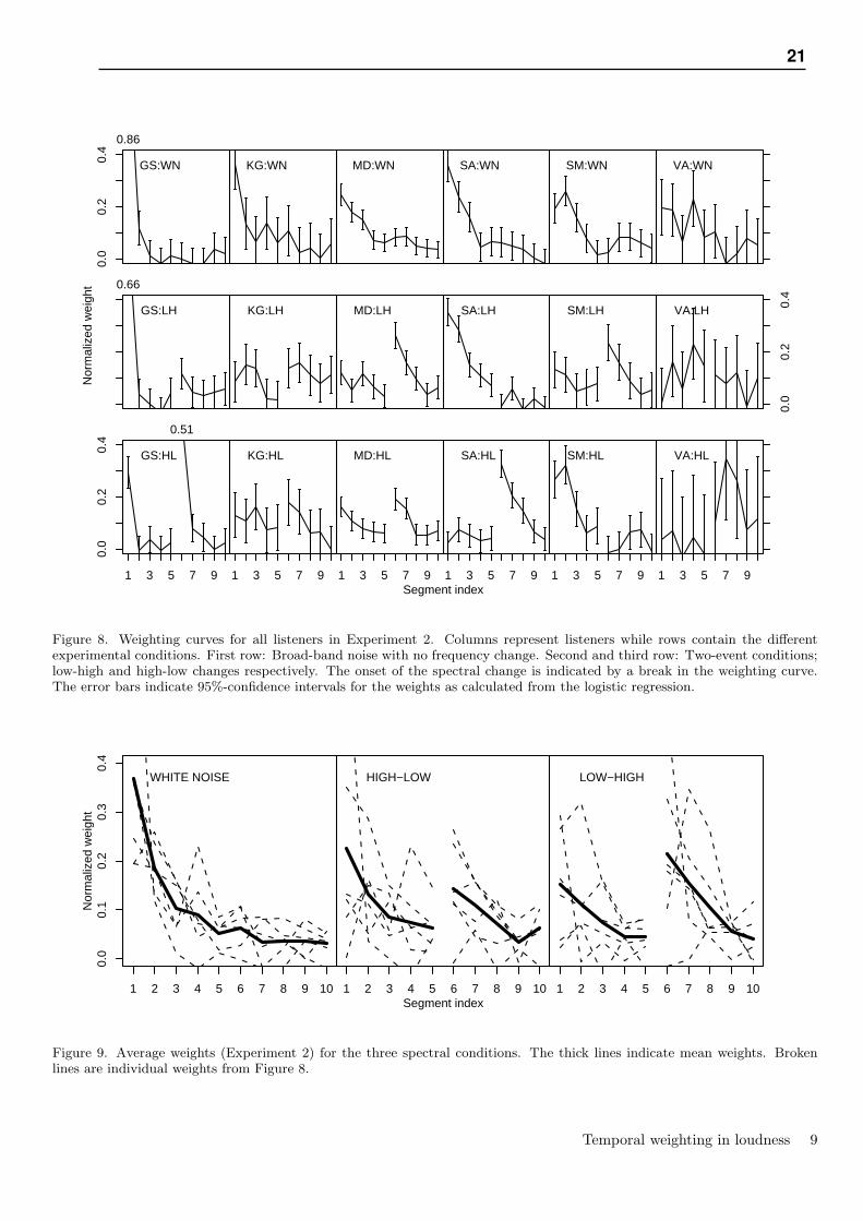
0.0

0.2

0.4

0.0

0.2

0.4

1 3 5 7 9

0.0

0.2

0.4

1 3 5 7 9 1 3 5 7 9 1 3 5 7 9 1 3 5 7 9 1 3 5 7 9

GS:WN

0.86

KG:WN MD:WN SA:WN SM:WN VA:WN

GS:LH

0.66

KG:LH MD:LH SA:LH SM:LH VA:LH

GS:HL

0.51

KG:HL MD:HL SA:HL SM:HL VA:HL

Segment index

Nor

mal

ized

wei

ght

Figure 8. Weighting curves for all listeners in Experiment 2. Columns represent listeners while rows contain the differentexperimental conditions. First row: Broad-band noise with no frequency change. Second and third row: Two-event conditions;low-high and high-low changes respectively. The onset of the spectral change is indicated by a break in the weighting curve.The error bars indicate 95%-confidence intervals for the weights as calculated from the logistic regression.

1 2 3 4 5 6 7 8 9 10

0.0

0.1

0.2

0.3

0.4

1 2 3 4 5 6 7 8 9 10 1 2 3 4 5 6 7 8 9 10

HIGH−LOW LOW−HIGHWHITE NOISE

Segment index

Nor

mal

ized

wei

ght

Figure 9. Average weights (Experiment 2) for the three spectral conditions. The thick lines indicate mean weights. Brokenlines are individual weights from Figure 8.


21

sound to be stored in memory in a simple sequential way.Whether assumptions about “resetting” the onset detec-tor, or separate storage of the two spectral events mightremedy the situation, is doubtful.

IV. FINAL DISCUSSION AND CONCLUSION

The results of the present experiments appear incom-patible with the notion of an automatic, accumulative in-tegration process as hypothesized by most loudness mod-els (e.g. Glasberg and Moore, 2002; Zwicker, 1977). Amajor outcome of these loudness models is to generatea continuous loudness curve, which is to account for theresults of e.g. temporal masking experiments and sub-jective loudness matches of modulated sounds. But topredict how listeners arrive at global loudness judgmentsrequires further stating how this continuous curve is “in-tegrated” to produce a single judgment. The presentdata address both of these stages.

In the calculation of a continuous loudness curve, allcurrent models operate with some sort of temporal sum-mation with a critical time coefficient in the range from20 ms to 50 ms depending on whether the loudness curveis rising or falling (Glasberg and Moore, 2002; Grimmet al., 2002; Zwicker, 1977). It is therefore impossiblefor loudness determined by these models to fluctuate anyfaster than the time coefficients allow. The fact thatin the present experiment, for some listeners, adjacentsegments were weighted very differently (see Figure 3),implies that their “continuous loudness” must fluctuateat least as rapidly as the segment duration of the sounds(100 ms) or else a particular segment could not be “sin-gled out” receiving extra weight. Thus, though the timecoefficients of the models are not in direct contradictionwith the observed weighting patterns, there is some in-dication that the integration taking place is not a simple“smoothing” process. In their loudness model, Glasbergand Moore (2002) introduce a further stage of determin-ing “long-term” loudness, with integration coefficients ofapproximately 100 ms for rising and 2000 ms for fallingloudness. These long time coefficients are not compatiblewith the results of the present experiments.

When it comes to integrating the sensory informationinto a loudness judgment, the present experiments pro-vides further evidence against the operation of simpleloudness integration:

(1) Weights derived for the 10 temporal segments de-fined were not uniform, but rather, in the unbi-ased, non-feedback conditions of Experiment 1 and2, provided evidence for perceptual emphasis of on-sets and offsets. That is not predicted by any ofthe current loudness models. Nor is it predictedby practical measurement rules (e.g. Zwicker andFastl, 1999) that assume values close to the maxi-mum (e.g. the 4th percentile Grimm et al., 2002;Zwicker and Fastl, 1999) to determine the loudnessof a time-varying sound. All of these rules would,

for the randomly varying sounds used in the presentexperiments, imply “flat” weighting curves to re-sult.

(2) When trial-by-trial feedback was provided inExperiment 1, listeners adapted their temporalweights to approach an optimal, uniform weight-ing of all stimulus segments. Such a “learning ef-fect” is hard to reconcile with the notion of an auto-matic integration process operating in the auditoryperiphery with a relatively long time coefficient.Rather, the listener must have access to some rep-resentation of the segment loudnesses (prior to in-tegration) with a finer resolution than the segmentduration in order to modify weights to maximizethe percentage of “correct” responses.

(3) When a qualitative change was introduced into thenoise sequence by switching the spectrum from alow-pass to a high-pass characteristic (or vice versa)in Experiment 2, listeners strongly weighted theonset of the “new” sound feature, thus boostingweights in the central portion of the compositestimulus. That is inconsistent with temporal wide-band energy integration which would be “blind”to the spectral change; it is also inconsistent witha memory explanation based on a “primacy” and“recency” advantage.

(4) All of the weighting patterns observed exhibitedconsiderable inter-individual variability. That initself argues against a low-level integration mecha-nism, which one would not assume to leave degreesof freedom for individual idiosyncrasies. Ratherit suggests some cognitive process to be involved,which can be controlled by the listener to some ex-tent.

What then are the alternatives for understanding theweighting of level information, and its adaptability tovarious listening conditions? It appears that, in the timerange of several hundred milliseconds investigated here,different stimulus segments must be individually acces-sible, granting the listener “multiple looks” (Viemeisterand Wakefield, 1991) on a temporal loudness pattern.Depending on the task requirements (Experiment 1) oron stimulus features (the spectral changes in Experiment2), these “looks” may be weighted differently, under im-plicit control by the listener. The particular salience ofonsets and offsets, as well as qualitative changes in thestimulus, may be due to mechanisms of memory, or morelikely to the “distinctiveness” (Neath, 1993; Neath et al.,2006) of these events in relation to other stimulus com-ponents, thereby attracting greater perceptual weight.

How could these hypotheses be put to further tests? Ifmemory was a factor, one might expect the timing of theevent sequence to play a crucial role. Furthermore, to ex-plore the “distinctiveness” concept, salient changes otherthan spectral ones (e.g. spatial lateralization) might beexplored, or an event could be generated by switching


22 Paper 1

from coherent to incoherent noise samples of the carriersignal across the two ears. Potentially, the segment lev-els could also be different across the ears, providing ameans to examine both temporal and binaural loudnesssummation.

Hopefully, based on such research, a clearer picture willemerge, on how the loudness of time-varying sounds isdetermined by both perceptual and cognitive processes.

V. ACKNOWLEDGMENTS

We would like to thank Florian Wickelmaier for help-ful hints regarding the statistical analysis of the results.This research was carried out as part of the “Centercon-tract on Sound Quality” which establishes participationin and funding of the “Sound Quality Research Unit”(SQRU) at Aalborg University. The participating com-panies are Bang & Olufsen, Bruel & Kjær, and DELTAAcoustics & Vibration. Further financial support comesfrom the Ministry for Science, Technology, and Develop-ment (VTU), and from the Danish Research Council forTechnology and Production (FTP).

(1) Non-integer degrees of freedom results sincea Welch-Satterthwaite approximation was used,which means that same variance for the weights inthe feedback and no-feedback group is not assumed

Berg, B. G. (1989). “Analysis of weights in multiple observa-tion tasks”, J. Acoust. Soc. Am. 86, 1743–1746.

Buus, S. (1999). “Temporal integration and multiple looks,revisited: Weights as a function of time.”, J. Acoust. Soc.Am. 105, 2466–2475.

Buus, S., Florentine, M., and Poulsen, T. (1997). “Tempo-ral integration of loudness, loudness discrimination, and theform of the loudness function.”, J. Acoust. Soc. Am. 101,669–680.

Cohen, J. (2003). Applied multiple regression/correlationanalysis for the behavioral sciences, 3rd edition (LawrenceErlbaum, Mahwah, NJ).

Doherty, K. A. and Lutfi, R. A. (1996). “Spectral weights foroverall level discrimination in listeners with sensorineuralhearing loss.”, J. Acoust. Soc. Am. 99, 1053–1058.

Doherty, K. A. and Lutfi, R. A. (1999). “Level discriminationof single tones in a multitone complex by normal-hearingand hearing-impaired listeners.”, J. Acoust. Soc. Am. 105,1831–1840.

Ellermeier, W. and Schrodl, S. (2000). “Temporal weightsin loudness summation”, in C. Bonnet (Ed.), Fechner Day2000. Proceedings of the 16th annual meeting of the Interna-tional Society for Psychophysics, 169–173 (Universite LouisPasteur, Strasbourg).

Glasberg, B. R. and Moore, B. C. J. (2002). “A model ofloudness applicable to time-varying sounds”, J. Audio Eng.Soc. 50, 331–342.

Grimm, G., Hohmann, V., and Verhey, J. L. (2002). “Loud-ness of fluctuating sounds”, Acust. Acta Acust. 88, 359–368.

Kortekaas, R., Buus, S., and Florentine, M. (2003). “Percep-tual weights in auditory level discrimination.”, J. Acoust.Soc. Am. 113, 3306–3322.

Lutfi, R. A. (1990). “Informational processing of complexsound. II. Cross-dimensional analysis.”, J. Acoust. Soc. Am.87, 2141–2148.

Lutfi, R. A. (1995). “Correlation-coefficients and correla-tion ratios as estimates of observer weights in multiple-observation tasks”, J. Acoust. Soc. Am. 97, 1333–1334.

McFarland, D. J. and Cacace, A. T. (1992). “Aspects ofshort-term acoustic recognition memory: modality and ser-ial position effects.”, Audiology 31, 342–352.

Moore, B. C. J. (2003). An Introduction to the Psychology ofHearing, 5th edition (Academic Press, San Diego, CA).

Neath, I. (1993). “Distinctiveness and serial position effectsin recognition.”, Mem. Cognit. 21, 689–698.

Neath, I., Brown, G. D. A., McCormack, T., Chater, N., andFreeman, R. (2006). “Distinctiveness models of memoryand absolute identification: evidence for local, not global,effects.”, Q. J. Exp. Psychol. 59, 121–135.

Saberi, K. (1996). “Observer weighting of interaural delaysin filtered impulses.”, Percept. Psychophys. 58, 1037–1046.

Southworth, C. and Berg, B. G. (1995). “Multiple cues forthe discrimination of narrow-band sounds”, J. Acoust. Soc.Am. 98, 2486–2492.

Stecker, G. C. and Hafter, E. R. (2002). “Temporal weightingin sound localization.”, J. Acoust. Soc. Am. 112, 1046–1057.

Surprenant, A. M. (2001). “Distinctiveness and serial posi-tion effects in tonal sequences.”, Percept. Psychophys. 63,737–745.

Tang, Z., Richards, V. M., and Shih, A. (2005). “Comparinglinear regression models applied to psychophysical data”, J.Acoust. Soc. Am. 117, 2597.

Viemeister, N. F. and Wakefield, G. H. (1991). “Temporalintegration and multiple looks.”, J. Acoust. Soc. Am. 90,858–865.

Willihnganz, M. S., Stellmack, M. A., Lutfi, R. A., and Wight-man, F. L. (1997). “Spectral weights in level discriminationby preschool children: synthetic listening conditions.”, J.Acoust. Soc. Am. 101, 2803–2810.

Zwicker, E. (1977). “Procedure for calculating loudnesss oftemporally variable sounds.”, J. Acoust. Soc. Am. 62, 675–682.

Zwicker, E. and Fastl, H. (1999). Psychoacoustics: Facts andmodels (Springer, Berlin).


23

Chapter 3

Modeling level discrimination:Non-linear and across-trial effects

3.1 IntroductionPrevious analyses (Pedersen and Ellermeier, 2006) showed how listeners weight the temporal compo-nents of a sound when judging its overall loudness. The analysis required two assumptions: (1) Whenmaking a loudness judgment, the listeners consider each trial in isolation, and (2) the loudness judg-ment is based on a linear weighting of the ten segments constituting a single sound. There are severalreasons why these assumptions may not by justified:

• A loudness judgment does not just depend on the stimulus presented on a given trial.

• Specifically, a judgment may depend on the “history” of the sounds encountered (DeCarlo andCross, 1990): Listeners may learn and change behavior throughout the experiment or they maybe unable to consider a sound of a given trial in complete isolation from the sounds presented onprevious trials.

• Furthermore, listeners’ decisions may be influenced certain statistics of the sound exposure: Themaximum sound level of a sound may determine its judged loudness or the variability of thesound pressure level within a trial may have an effect.

This chapter will address questions like these. The chronology of the chapter is to examine first towhich extent loudness judgments do not depend on the sound of a single trial only. To that end, severalaspects are considered: (1) Effects which do not directly depend on the sound level (bias toward either“loud” or “soft” or special response patterns (alternating “loud”/”soft” responses for example)). (2) Itwill be demonstrated how the loudness judgment on a given trial depends on the levels presented onprevious trials. In following sections it will be examined how listeners may process information ofsingle trials before arriving at a loudness judgment. To that end, first some empirical observations aresummarized, where the statistical probability of a given response as a function of the segment levels ofa given sound is analyzed. This will help to identify important aspects, which a model of the decisionprocess must be able to account for. In the following, several suggestions for modeling the decisionprocess are given. First, the ability of two of the more established theories for temporal integration inhearing (model of temporal loudness integration by Glasberg and Moore (2002) and temporal windowmodel by Oxenham and Moore (1994)) to predict the behavior of listeners is examined. As thesestwo models do not seem to explain the behavior of the listeners, a range of models are formulatedmathematically and fitted to the responses of the listeners. The ability of the fitted models to predictthe listeners’ behavior are then compared to identify which models include important aspects of thedecision process.

26 Non-linear and across-trial effects

It has been demonstrated that reaction time is related to loudness (Wagner et al., 2004), thereforethe response time of the listeners is also analyzed. This reveals a strong correspondence between soundlevel and response time, but not in a way which can be simply related to the listeners’ actual loudnessjudgments. In spite not being directly related to loudness, the response time analysis gives insight intothe complexity of the decision process.

The chapter ends with analyzing temporal weights in a task where listeners had to compare theloudness in pairs of level-fluctuating sounds (Ellermeier and Schrödl, 2000). This extends the analysisto also examine how listeners handle several integrated loudness impressions in a comparison task.

If not stated otherwise, all results presented in this chapter are based on the data obtained in Ex-periment 1 of the present thesis (Pedersen and Ellermeier, 2006). Potentially, the same analyses couldalso be applied to the results of Experiment 2 of the thesis, but this has been avoided to maintain aclear focus throughout the chapter and because of the larger amount of data collected for each listenerin Experiment 1 allowing for greater statistical power.

The overall goal of this chapter is to arrive at conclusions about the factors involved in the temporalintegration of loudness, extending the study presented in the previous chapter by not assuming thatloudness judgment is based on a simple linear (weighted) summation of segment levels.

3.2 Effects across trialsIn the previous chapter it was assumed that a listener’s “soft” or “loud” response depended only on theten segment levels of the trial in question. There are, however, several reasons why listeners may notalways behave in accordance with this assumption:

• Response category bias - When a listener is uncertain about the response he/she may use onlyone type of answer like an “I don’t know” category.

• Persistence of response bias - A listener may feel uncomfortable pressing the same button manytimes in a row even though a long series of the same response might be correct.

• Unstable decision criterion - Listeners need a reference to discriminate “loud” and “soft”, andthis reference may for example depend on the levels of the sounds of previous trials.

• Effects of learning - The listener may get better throughout the time-course of the experiment orchange his/her decision criterion.

In the following, the listeners’ behavior will be analyzed in an attempt to clarify the questionsraised.

3.2.1 Level-independent effectsResponse category bias

All listeners are biased toward answering either “loud” or “soft” as summarized in Table 3.1. The tablesimply gives the overall percentage of “loud” responses. When assuming a binomial distribution of theresponses, then the estimated probability of “loud” is identical to the percentage of “loud” judgmentsand the confidence intervals for its estimated value can be calculated. The bias may not always beindependent of level, if for example a listener applies a relatively low “reference level” in his/herjudgments, the amount of “loud” responses will be higher than the amount of “soft” responses. Thistype of bias is accounted for in the modeling as described in section 3.5, and only level-independentbias is of concern here. Discriminating these two types of bias is not easily done, since listeners didnot give any reason why they made a given decision.

Effects across trials 27

BB BJ BP CP JJ BL EH JV LH WEPercent “loud” 54.0 56.5 53.9 55.9 48.3 47.5 52.3 53.5 60.2 54.0p-value ∗∗∗ ∗∗∗ ∗∗∗ ∗∗∗ 0.024 0.001 0.002 ∗∗∗ ∗∗∗ ∗∗∗

Table 3.1: Response category bias. Each listener’s percentage of “loud” responses in the first rowand, in the bottom row, the probability that this could have occurred if the real probabilityof “loud” was 50% (p-value, two-tailed binomial test). “∗∗∗” indicates p < 0.001.

Persistence of response bias

A listener may feel uncomfortable about pressing the same button many times in a row, or may contin-uously press the same button if he/she is not certain of the responses. In either case a given responsewill depend on the listener’s earlier responses. Calculating the autocorrelation sequence of a listener’sresponses at different lags can be used to estimate this effect. For example at a lag of one, the auto-correlation shows how likely it is that a listener’s current response will be the same as the previous,where the correlation coefficient ranges from -1 (the listener’s responses are always opposite in twoconsecutive trials) to 1 (the listener’s responses are always the same in two consecutive trials). A moredetailed description is for example given by Venables and Ripley (2002). The autocorrelation sequencefor the responses is shown for each listener in Figure 3.1. It should be noted that some trials in thecalculation of the autocorrelation sequence occurred in different blocks in the listening experiment.For example, at a lag of one, the first trial of a block is compared to the last trial of the previous block.This comparison may not be relevant, but it happens relatively seldom that the two trials compared fallinto different blocks.

−0.

3−

0.1

0.1

0.3

0 2 4 6 8 0 2 4 6 8 0 2 4 6 8

−0.

3−

0.1

0.1

0.3

Lag [Nr of trials]

Aut

ocor

rela

tion

●

●

●

●●

● ● ●●

● ●●

●

●

● ● ●● ● ● ● ● ● ● ●

● ●● ● ● ●

●●

●●

●

BB

●

●

● ● ●● ●

● ●●

● ●●

●●

●● ●

●

● ● ● ●●

●● ●

●●

● ●● ● ● ●

●

BJ

●

●

●

●● ●

●● ● ●

●● ●

●●

● ● ●●

●● ●

●●

●●

●

● ●●

●●

BP●

●

●●

●

● ●● ● ● ●

● ● ●● ● ●

● ●● ●

●

CP

●

●●

● ● ●●

●

●

●● ●

JJ●

●● ●

● ● ● ●●

●

●

●

●● ●

●● ●

●

●

●●

● ●●

●

●●

●

●●

●●

●● ● ●

BL

●

●

●●

● ●

● ● ● ● ●●

●● ●

● ●● ●

● ● ● ●●

●● ●

● ●● ● ●

● ●

●

●●

EH

●

●●

●● ●

● ●● ● ●

●● ● ● ● ●

● ● ●

●

●●

●●

●●

● ●● ●

● ●

JV

●

●

●

●

●

●●

●

●● ●

●

●● ● ● ●

●● ●

●

●

●

LH

●

●

●● ●

●●

●●

●●

●

●

WE

Figure 3.1: Autocorrelation sequences for the responses of each individual listener. The lag is indi-cated on the x-axis, and at a lag of 1 the value on the y-axis indicates how a listener’sprevious response correlates with the response of the current trial. Top: Listeners notreceiving feedback; bottom: Listeners receiving feedback.

The order of generated “loud” and “soft” sounds was random in the experiment, meaning that theautocorrelation sequence of the generated stimuli is 0 for any lag different from 0. Thus, ideally, theautocorrelation sequence of a listener’s responses should also be 0. From Figure 3.1 it is seen that thisis not the case for all listeners. On a given trial listener JJ is likely to give the opposite response as inthe previous trial (large negative correlation coefficient at a lag of 1) and listener CP is likely to give the


same response in two (or even three) consecutive trials (positive correlation coefficients at a lag of 1,2,and 3). Listener LH seems to give alternating responses. It could be hypothesized that listeners benefitfrom feedback to avoid this behavior, because the feedback would “tell” them that sometimes multiplesounds of the same category occur in a row. Further they may notice how often a given type of sound(“soft” or “loud”) occurs in a row and how often this happens and adapt their behavior accordingly. Itis therefore of interest to determine to which extent listeners are able to adapt to the “statistics” of thesignal generation. This may be done in the following way: All responses of a listener are considered intheir presented order. On this list it can be counted how often the listener gives sequences of the sameresponse in a row. To understand this consider the following series of responses:

loud, soft, soft soft, loud, soft

On this list there is one occurrence of “soft” in a sequence of 3, one occurrence of “soft” in a sequenceof 1 and 2 occurrences of “loud” in a sequence of 1. The responses of all listeners were analyzed thisway and the results are shown in Figure 3.2. Each count was multiplied by the length of the relevantsequence, so for example the 3 “soft” in a row in the example, would contribute with a value of 3to the y-value at the “3-soft-in-a-row” category. This makes the total sum of the y-values equal tothe number of trials. The figure also shows (as a solid line) the behavior of a model giving a “loud”response when the mean level of the segments of a sound is bigger than the overall mean and “soft”response if it is less. The line thus represents the “statistics” of the signal generation. From the figureit is seen that listeners in the feedback group generally behave in accordance with the “statistics ofgeneration” curve except for LH’s “soft” responses for which it is seen that LH hesitates to press “soft”in longer sequences. In the no-feedback group people generally deviate from the “statistics” curve.BP, CP, and JJ deviate most where JJ is reluctant to give the same response many times in a row andCP gives the same response in a row too often. BP often gives the same response two times in a row.BB and BL give continuous “loud” responses too often. In summary, people in the feedback groupseem to “statistically” adapt to the feedback. It should be noted that this form of adaption does notgive any benefit in obtaining better performance scores since the segment levels on different trials areuncorrelated.

3.2.2 Level dependent effects across trials

Weighting contrasts

For each response a listener gives he/she needs a reference for the judgment. For example the listenermay have a good impression of the overall mean level of all sounds or the listener could simply comparethe level of the sound of the current trial to that of the previous. The latter can be tested for theweighting model, if the prediction of a response is based on segments across several trials. Considerthe following model for example:

L(x) =10

∑i=1

w0,ix0,i +10

∑i=1

w1,ix1,i +10

∑i=1

w2,ix2,i

The weights w0,i are weights put on the segments of the current trial while w1,i are weights put onthe previous trial and w2,i are weights put on the trial before that. The weights were fitted as describedby Pedersen and Ellermeier (2006). The fitted weights are shown for all listeners in Figure 3.3.

Ideally, only the weight put on the segments of the current trial should be different from 0, since thetask of the listener is to judge only the sound of a single trial. Listener BP and JJ deviate most from thisin that they seem to contrast levels of previous trials with levels of the current, maintaining the sameshape of the weighting curve, but with opposite sign. It can be observed that, in absolute measures,some heavily weighted segments of previous trials are more important than weakly weighted segments

Effects across trials 29

020

060

0

1 3 5 7 9 1 3 5 7 9 1 3 5 7 9

020

060

0

Nr of same response in a row

Tot

al n

r of

res

pons

es

●

●●

●

●

●●

●●

● ● ● ● ● ● ● ● ● ● ● ● ● ● ● ● ● ● ● ● ● ● ● ● ● ● ● ● ● ● ● ● ● ● ● ● ● ● ● ●

BB

●

●

●

●

●

● ●●

● ●● ● ● ● ● ● ● ● ● ● ● ● ● ● ● ● ● ● ● ● ● ● ● ● ● ● ● ● ● ● ● ● ●

BJ

●

●

●

●

●

●●

● ● ● ● ● ● ● ● ● ● ● ● ● ● ● ● ● ● ● ● ● ● ● ● ● ●

BP

● ● ●

●●

● ●

●

●●

●●

●● ● ● ● ● ● ● ● ● ●

CP ●

●

●

●

● ● ● ● ● ● ● ● ●

JJ

●

●

●

●

●

●●

●● ●

● ● ● ● ● ● ● ● ● ● ● ● ● ● ● ● ● ● ● ● ● ● ● ● ● ● ● ● ● ● ● ● ● ● ● ● ● ● ●

BL

●

●

● ●

●

●●

● ● ● ● ● ● ● ● ● ● ● ● ● ● ● ● ● ● ● ● ● ● ● ● ● ● ● ● ● ● ● ● ● ● ● ●

EH

●●

●

●

●

●

●●

● ●● ● ● ● ● ● ● ● ● ● ● ● ● ● ● ● ● ● ● ● ● ● ●

JV

●

● ●

●

●●

● ● ●● ●

● ● ● ● ● ● ● ● ● ● ● ●

LH

●

●

●

●

●

●●

●● ● ● ● ●

WE

Figure 3.2: Frequencies of same response in a row for individual listeners. The x-axis indicates thepossible numbers of same response in a row. Circles correspond to “loud” responses ina row and triangles “soft”. The y-axis shows the number of trials falling in series of lengthas indicated on the x-axis. If for example a listener gives three “loud” responses in a rowthis will contribute with a count of 3 for the circle at an x-value of “3 in a row”. The sumof all “circle and triangle”-values is equal to the total number of trials. The line shows the“behavior” of a simple model making judgments based on the mean value of the levelsof the segments. Listeners not receiving feedback in the top row and listeners receivingfeedback in the bottom row.

Index

0

−0.

100.

050.

15

Index

0

Index

0

Index

0

Index

0

Index

0

1 3 5 7 9

Index

0

Index

0

1 3 5 7 9

Index

0

Index

0

1 3 5 7 9

−0.

100.

050.

15

0

0 0 00

00 0

00

11

1 1 11 1

11

12 2 2 2 2 2 22 2 2

BB0 0

00

0 0 0 0 0

0

11 1 1 1

1 1 1 112 2 2

22 2 2 2 2

2

BJ

0

0

0 00 0

0 0 0 0

1 11 1 1 1 1 1 1

1

2 22 2 2 2 2 2 2 2

BP 00

0 0 0 0 00 0

1 11

11

1 1 11

12 2 2 2 2

2 2 2 2 2

CP

0

00 0 0 0 0 0

0

0

1

1 1 1 1 11 1 1 1

2 2 22 2 2 2

2 2 2

JJ

0

00

00

0 00 0

0

1 11 1 1 1

11 1 12 2 2 2 2

2 2 22 2

BL

0 0 0 0 0 0 0 0 0 0

1 1 1 1 1 1 1 1 1 12 2 2

22 2 2 2 2 2

EH

0 0 0 00 0 0 0 0 0

1 1 1 1 1 1 1 1 112 2 2 2 2 2 2 2 2 2

JV 0 0 0

00 0 0

0 00

11

11 1 1

1 11 12 2 2 2 2 2

2

22 2

LH0

0 0 0 0 00 0 0 0

1 1 1 1 1 1 1 1 11

2 2 2 2 2 2 2 2 2 2

WE

Segment index

Nor

mal

ized

wei

ght

Figure 3.3: Weighting contrasts for individual listeners across three trials. All weights are scaled bythe same factor chosen so the sum of the weights of curve “0” is 1. The numbers on thecurves indicate the lag in relation to the current trial.


of the current trial. In the feedback group this behavior is not observed to the same extent. This couldbe an indication that feedback is helpful for maintaining a fixed reference level for the judgments.

3.2.3 Changes in weighing curve as a function of time

It may be of concern whether the listeners maintain the same weighting curves throughout the entireexperiment, or they change over time. This is especially interesting for the listeners in the feedbackgroup as it may seem plausible that they slowly changed their weighting according to the feedback. Inan attempt to graphically examine this, weighting curves were derived from data obtained in differentphases of the experiment as a function of time from the beginning of the experiment toward the end.The obtained data for each listener were divided into ten overlapping portions. The results of 1000trials were included in each portion. The total amount of trials per listener was 4598 so approximately5 independent estimates of each listener were obtained for different phases of the experiment. All trialswere sorted according to their index in time in the total series of trials, and from the sorted list of trialsthe portions were picked. 10 different estimates of the weighting curves were made for each listeneras a function of index, so for example the first estimate of weights is based on the 1000 first judgmentsmade by a given listener and the next estimate is based on trial number 400 to 1399. The weightingcurves for all listeners are shown in Figure 3.4, where different listeners are shown in different columnsand their weighting curves for the different phases of the experiment are shown in different rows. Theweighting curves were calculated as described by Pedersen and Ellermeier (2006).

The main conclusion of inspecting Figure 3.4 is that listeners to a large extent maintain the sameweighting pattern throughout the experiment. Only one listener, JV, behaves according to the hypothe-sis that listeners in the feedback group get closer to “optimal” weighting throughout the experiment. Inthe beginning listener JV emphasized the end of the sound, where as, at the end of the experiment, JV’sweights are nearly “flat”. The relatively stable weighting patterns indicate that the weighting curve issettled before the experiment proper, potentially in the initial training.

3.3 Modeling the decision processIn our earlier work on temporal weights (Pedersen and Ellermeier, 2006), listeners were always as-sumed to give loudness judgments based on the weighted sum of the 10 segments of a given sound.This analysis revealed that listeners apply very different individual weights. It has, however, not beenshown that the temporal weighting is the only factor involved in the decision process. There havebeen different suggestions in the literature for how listeners arrive at an overall judgment of loudness:Moore et al. (2003) propose a simple mean of the loudness curve (similar to the case where all temporalweights are equal), and Zwicker and Fastl (1999) propose that the level exceeded a certain percentile ofthe time is decisive for loudness judgments, further elaborated on by Grimm et al. (2002). More com-plex aspects have been found to be involved in listening experiments: Stecker and Hafter (2000), forexample, found that ramped sounds are perceived louder that damped sounds, and Oberfeld and Plank(2005) found that, in judging loudness of sounds slowly fading in, listeners emphasized the temporalsegment where fading ended.

Because of the random segment variation of the sounds used in the experiment, the sounds posses,and to different degrees, many of the properties found to be influential. Therefore it seems worthwhileto examine how different concepts help in explaining the performance of the listeners.

3.3.1 Model-independent observations

Before turning to the description of specific models, there are a number of observations, which canbe made independently from assumptions about the decision process, and which provide insight into

Modeling the decision process 31

Index

0

0.0

0.2

0.4

Index

0

Index

0

Index

0

Index

0

Index

0

Index

0

Index

0

Index

0

Index

0

Index

0

Index

0

Index

0

Index

0

Index

0

Index

0

Index

0

Index

0

Index

0

Index

0

0.0

0.2

0.4

Index

0

0.0

0.2

0.4

Index

0

Index

0

Index

0

Index

0

Index

0

Index

0

Index

0

Index

0

Index

0

Index

0

Index

0

Index

0

Index

0

Index

0

Index

0

Index

0

Index

0

Index

0

Index

0

0.0

0.2

0.4

Index

0

0.0

0.2

0.4

Index

0

Index

0

Index

0

Index

0

Index

0

Index

0

Index

0

Index

0

Index

0

Index

0

Index

0

Index

0

Index

0

Index

0

Index

0

Index

0

Index

0

Index

0

Index

0

0.0

0.2

0.4

Index

0

0.0

0.2

0.4

Index

0

Index

0

Index

0

Index

0

Index

0

Index

0

Index

0

Index

0

Index

0

Index

0

Index

0

Index

0

Index

0

Index

0

Index

0

Index

0

Index

0

Index

0

Index

0

0.0

0.2

0.4

Index

0

0.0

0.2

0.4

Index

0

Index

0

Index

0

Index

0

Index

0

Index

0

Index

0

Index

0

Index

0

Index

0

1 4 7

Index

0

Index

0

1 4 7

Index

0

Index

0

1 4 7

Index

0

Index

0

1 4 7

Index

0

Index

0

1 4 7

Index

0

0.0

0.2

0.4

BB:1

BB:2

BB:3

BB:4

BB:5

BB:6

BB:7

BB:8

BB:9

BB:10

BJ:1

BJ:2

BJ:3

BJ:4

BJ:5

BJ:6

BJ:7

BJ:8

BJ:9

BJ:10

BP:1

BP:2

BP:3

BP:4

BP:5

BP:6

BP:7

BP:8

BP:9

BP:10

CP:1

CP:2

CP:3

CP:4

CP:5

CP:6

CP:7

CP:8

CP:9

CP:10

JJ:1

JJ:2

JJ:3

JJ:4

JJ:5

JJ:6

JJ:7

JJ:8

JJ:9

JJ:10

BL:1

BL:2

BL:3

BL:4

BL:5

BL:6

BL:7

BL:8

BL:9

BL:10

EH:1

EH:2

EH:3

EH:4

EH:5

EH:6

EH:7

EH:8

EH:9

EH:10

JV:1

JV:2

JV:3

JV:4

JV:5

JV:6

JV:7

JV:8

JV:9

JV:10

LH:1

LH:2

LH:3

LH:4

LH:5

LH:6

LH:7

LH:8

LH:9

LH:10

WE:1

WE:2

WE:3

WE:4

WE:5

WE:6

WE:7

WE:8

WE:9

WE:10

Segment index

Nor

mal

ized

wei

ght

Figure 3.4: Changes in weighting curves for all listeners in different columns. The weighting curvesare fitted to responses in different phases of the experiment as indicated in the upper leftcorner of the graphs and changing across the rows. “1” indicates the first phase of theexperiment and “10” the last. The first 5 listeners, from left to right, are the listeners in theno-feedback group. Error bars indicate plus/minus one standard deviation as calculatedin the logistic regression.


which aspects a model must be able to account for.

Smoothing curves

For visual presentation of results a smoothing function will be extensively used throughout this chap-ter, so the following short-hand notation is introduced:

Y (X)nr_intervals,nr_in_interval

Here Y depends on X , where Y is a vector of observations at physical levels given by the valuesof the vector X . The expression tells that Y and X have been smoothed according to the (integer)subscripts (nr_intervals and nr_in_interval) in the following way:

(1) X is sorted in ascending order.

(2) If elements were reordered in X , a similar reordering is made of the elements of Y .

(3) X is divided into nr_intervals (potentially overlapping) intervals, so there are nr_in_intervalelements in each interval. The intervals are equidistant in term of their index in the sorted vectorX . The first interval contains the first elements of the sorted X and the last interval contains thelast elements of the sorted X .

(4) For each interval the mean value of the nr_in_interval elements is calculated. The calculatedvalues are the “smoothed” X .

(5) Similarly, mean values are calculated for intervals of Y , which are then the “smoothed” Y .

The confidence interval of the estimated mean of the values of Y in a given interval can be calculatedusing a simple t-test. If the values have a binomial nature a confidence interval can be calculated basedon the binomial distribution.

Non-linearity as a function of overall level?

For the segment levels used in the experiment (60 dB to 75 dB SPL), loudness is almost linearly relatedto the sound pressure level in decibels for steady-state sounds (see for example Moore, 2003a). Still, itmay be of concern whether the overall (mean) level of a sound is linearly related to the perceived level.Therefore the probability of a “loud” response has been depicted as a function of the mean level ofthe ten segments of a given sound in Figure 3.5. In the figure the gray-shaded area of 95% confidenceshows the actual “smoothed” responses for each listener. The solid line shows the best fitted curve(more carefully described in Chapter 3.5) relating the listener’s performance to a simple mean valueof the ten segment levels. A non-linear relation between response and segment levels would be seenas a systematic deviation of the solid curve from the “smoothed” performance. Seemingly there is nosignificant disagreement between the fitted curve and the listeners’ actual performance, thus it may beconcluded that there is not a significant non-linear term in the relationship between overall level andperceived level.

Conditioned on single segment (COSS) functions

The graphical illustration of the relation between response and overall level in Figure 3.5 is “blind”to effects concerned with single segments such as the first segment being more significant for thejudgment or there could be more complicated interaction effects. Inspired by the method describedby Berg (1989), the importance of each segment levels is examined. The method uses COSS function

Modeling the decision process 33

0.0

0.4

0.8

66 67 68 69 66 67 68 69 66 67 68 69

0.0

0.4

0.8

Mean segment amplitude [dB]

Por

tion

of "

loud

" r

espo

nses

BB BJ BP CP JJ

BL EH JV LH WE

Figure 3.5: Probability of “loud” as a function of mean level of the individual ten segment levels of asound. Response(xmean)25,250

(Conditional On Single Stimulus) to relate the level of each segment to the probability of a “loud”response. In the present work this is implemented by generating plots similar to those in Figure 3.5,but instead of having only one plot per listener, one plot per listener per segment is generated, wherethe x-axis denotes the sound pressure level of the relevant segment only. In Figure 3.6 such COSSfunctions are plotted for all listeners.

If listeners behaved according to a “linear” rule the COSS functions would be approximatelystraight lines with a slope indicating its significance relative to other segments (strictly speaking thisis only true when the COSS functions are transformed an accordance with the statistics of the signalgeneration). This does indeed seem to be the case for some listeners, EH and JV for example. Forothers (BB and BL for example) it does not seem to be the case. Especially for low segment levelsmany listeners seem to respond “loud” more often as would be assumed according to a linear model.As a rough summary of the results it can be stated that, when the level of a given segment is above acertain value (67.5 dB for example) it seems to contribute to the overall loudness in a way which iscompatible with a linear model, but when the level is below this value, it does not contribute as muchas would have been expected from a linear model, the reason being: When a segment level is belowthe overall mean (67.5) it is lower (on average) than other segments and the lower it is, it should makea “soft” response more likely. Some listeners, however, responds “loud” too often, which implies thatthe low segment level did not contribute as much as expected as to give a “soft” response. There is evensome weak evidence that for the lowest segment levels the probability of a “loud” response is higherthan for moderately higher levels (see segment 2 of BB in Figure 3.6 for example). In some cases thiswould imply that decreasing the level of a segment increases the probability of a “loud” response. Amodel, which is able to account for this is considered later.

Summary

In summary the presentation of the results in Figure 3.5 and 3.6 showed:

• In describing overall performance of listeners (Figure 3.5), a logistic curve (solid line in thefigure) followed the listeners responses well - no overall deviation was identified.


0.2

0.6

0.2

0.6

0.2

0.6

0.2

0.6

0.2

0.6

0.2

0.6

0.2

0.6

0.2

0.6

0.2

0.6

65 70 65 70 65 70 65 70 65 70

0.2

0.6

Segment amplitude [dB]

Por

tion

of "

loud

" r

espo

nses

BB1 BB2 BB3 BB4 BB5 BB6 BB7 BB8 BB9 BB10

BJ1 BJ2 BJ3 BJ4 BJ5 BJ6 BJ7 BJ8 BJ9 BJ10

BP1 BP2 BP3 BP4 BP5 BP6 BP7 BP8 BP9 BP10

CP1 CP2 CP3 CP4 CP5 CP6 CP7 CP8 CP9 CP10

JJ1 JJ2 JJ3 JJ4 JJ5 JJ6 JJ7 JJ8 JJ9 JJ10

BL1 BL2 BL3 BL4 BL5 BL6 BL7 BL8 BL9 BL10

EH1 EH2 EH3 EH4 EH5 EH6 EH7 EH8 EH9 EH10

JV1 JV2 JV3 JV4 JV5 JV6 JV7 JV8 JV9 JV10

LH1 LH2 LH3 LH4 LH5 LH6 LH7 LH8 LH9 LH10

WE1 WE2 WE3 WE4 WE5 WE6 WE7 WE8 WE9 WE10

Figure 3.6: Probability of “loud” as a function of level of single segments for all listeners,Response(xi)20,500. Regions of 95%-condidence are indicated. In the upper half (light-grey graphs) are listeners in the no-feedback condition and in the lower half (dark-grey)the listeners in the feedback condition. Listener ID and segment number indicated inthe upper left corner of each figure. The overall mean of all segment levels (67.5 dB) isindicated by a vertical broken line.

Applying a temporal loudness model 35

• Figure 3.6 revealed that for low segment levels, listeners responded “loud” more often (to differ-ent degrees) than expected from a linear model.

The fact that non-linear effects were identified to a larger extent for individual segments than forthe overall mean, suggests that the explanations lie in how loud a given segment is in relation to thelevels of other segments of a given sound. If for example all segment levels are low (giving a low meanvalue), listeners do not seem to press “loud” more often than would be expected from a linear model,but it is the case when only single segments are considered. The COSS functions for the nine lastsegments of listener BB (Figure 3.6) show that when a given segment’s level is below the overall mean(67.5 dB) he gives equally many “loud” and “soft” responses. This suggests that when a segment’slevel is sufficiently low, that segment is simply ignored by BB. Similar effects can be observed forother listeners, but to a smaller extent.

Explaining derived COSS functions

There are a number of reasons, which can be considered responsible for the non-linearity of the COSSfunctions:

(1) Temporal masking - If a high level of a segment persists in the sensory system over follow-ing softer levels, it could be argued that this causes the listener to press “loud” more often asexpected. This is however hard to reconcile with two observed facts: (1) Not all listeners re-sponded “loud” too often for low segment levels (EH and JV for example) and consequentlythere is no masking in their sensory system, and (2) the weighting curves derived by Pedersenand Ellermeier (2006) showed that adjacent segments can be weighted very differently, whichcould not be the case if there was a “smoothing” effect. Also, if the masking is mainly thoughtto be due to forward masking, only little (backward) masking would be expected for the firstsegment. This is indeed the case to some extent, but the first segment of for example WE doesnot appear to be less “masked” than following segments.

(2) Loudness percentile - The loudness exceeded a certain percentile of the time determines thelisteners’ response, and consequently the segment levels below this critical level has no influenceon the judgment.

(3) Attention - Louder segments (in relation to other segments of the same sound) catch more at-tention, and are thus weighted more heavily, which causes the listener to respond “loud” moreoften, as the softer segments do no catch the same attention.

The first of these point is examined in greater depth for the loudness model by Glasberg and Moore(2002) in Section 3.4. The two latter points are examined in Section 3.5, where various paradigms areapplied in an attempt to predict listeners’ loudness judgments.

3.4 Applying a temporal loudness model

In relation to the discussion of temporal masking given in the previous section there may be two typesof models to be considered: (1) Models predicting the loudness of time-varying sounds (Glasberg andMoore, 2002; Zwicker, 1977), and (2) models of temporal masking (as for example Oxenham andMoore, 1994). The two types of models will be addressed in the two following sections.


3.4.1 Evaluating models of time-varying loudnessThere are only few models, which are able to predict loudness of time-varying sounds. The earliestappears to be described by Zwicker (1977). In this work Zwicker mainly gives a description of themain principles of the model, and critical parameters (as for example the time coefficient for temporalintegration) are only given by reference to other work (suggestions for time coefficients are for examplegiven by Vogel (1975)). More recently, a computer program was described by Widmann et al. (1998),but the program is not a full loudness model, and only supposed to account for post-masking. The lackof a unified description of Zwicker’s model makes it hard to use it in practice. Therefore the focuswill be on the model given by Glasberg and Moore (2002), which also contains many of the elementsintroduced by Zwicker.

Glasberg and Moore’s model of time-varying loudness

Glasberg and Moore (2002) suggest how a model should integrate loudness over time to generate acurve of “continuous” loudness. Their suggestion for loudness integration is fundamentally an iterativeprocess, which they formulate as (Equation 1 and 3 of their paper):

S′n =

{αaSn +(1−αa)S′n−1 if Sn > S′n−1

αrSn +(1−αr)S′n−1 if Sn ≤ S′n−1(3.1)

This equation works on discretized “instantaneous” loudness (Sn), which in their formulation hasbeen sampled at a rate of 1 kHz (Ti = 1 ms). Subindices in the equation refer to index in the discretesequence. S′ is the integrated “short term” loudness sequence, and its definition is of a recursive natureas it appears from the equation where S′ is present on both sides of the equality. αa and αr of theequation indicate the integration rate, when the “short term” loudness curve is either rising (Sn > S′n−1)or falling (Sn ≤ S′n−1), and they are related to critical time coefficients of integration (Ta and Tr):αa = 1− e−Ti/Ta and αr = 1− e−Ti/Tr . Their suggested values are: αa = 0.045 and αr = 0.02, whichgives: Ta = 22 ms and Tr = 49 ms.

Further, Glasberg and Moore introduce the concept of “long term” loudness, which in its definitionis identical to Equation 3.1, except that “instantaneous” loudness, S, is substituted with “short term”loudness S′, “short term” loudness is substituted with “long term” loudness, S′′, and different integra-tion rates are used (αal = 0.01 and αrl = 0.0005). This corresponds to the time coefficients: Tal = 99ms and Trl = 2 s.

Glasberg and Moore suggest that “short term” loudness may account for aspects such as temporalmasking or persistence of neural activity in the auditory sensory system, while they use “long term”loudness to account for the results of experiments in which the loudness of modulated sounds wasjudged by listeners. It is not clear which type of loudness, “short term” or “long term”, would bemore relevant in describing the performance of the listeners in the task described by Pedersen andEllermeier (2006), therefore both “loudness” types will be applied to the stimuli of the experiment inthe following.

Conversion to sones

Before temporal integration is possible an “instant loudness” curve is needed. In the experiment de-scribed by Pedersen and Ellermeier (2006) the sound pressure levels were within the range from 60dB to 75 dB SPL. In this relatively narrow range the relationship between loudness in sone and soundpressure level in dB is close to linear. Consequently, Equation 3.1 might by directly applied to thestimuli of the experiment, where “instantaneous” loudness is given by the level of the ten individualsegments of a sound. But to stay as close as possible to Glasberg and Moore’s formulation of the modelas possible, all segment levels were transformed from values in dB to sone. The transformation was


made via the standard ANSI S3.4 (2005), which describes a procedure for the calculation of loudnessof stationary sounds given their amplitude spectra. A computer program for the calculation of loudnessaccording to the standard is freely available 1 and was used for the transform. The amplitude spectrumof a gives segment was supplied to the program by its spectrum level and bandwidth. The bandwidthwas always the full bandwidth supported by the program (20 Hz to 18 kHz) and in this range thespectrum level was assumed flat. The actual spectrum level was estimated by: SPL−10log(w), where“SPL” is the calibrated sound pressure level of a given sound segment as used in the experiment andw is the bandwidth of the noise (22 kHz) (Kinsler, 2000). The program for loudness calculations wasused in “diffuse field” mode, as the headphones were “diffuse field” compensated as described by themanufacturer.

Loudness integration of segment patterns

The result of loudness integration of the stimuli used by Pedersen and Ellermeier (2006) may be bestunderstood by graphical inspection of the generated loudness patterns, which are depicted in Figure3.7 (“short term”) and Figure 3.8 (“long term”). The curves were generated by sampling the “instanta-neous” loudness at a rate of 1 kHz and applying Equation 3.1.

05

1015

2025

30

Segment index

Loud

ness

[son

e]

1 2 3 4 5 6 7 8 9 10

Figure 3.7: Example of “short term” integrated loudness. “Instantaneous” loudness indicated by thebroken lines.

The graph in Figure 3.9 is identical to that of Figure 3.8, but Figure 3.9 shows the graph over awider time range. It is clear from the figures that “short term” loudness follows the “instantaneous”segment pattern quite closely, while in the case of “long term” loudness the curve continues for a longperiod after the end of the sound. “Long term” loudness is able to follow the “instantaneous” patternto some degree when loudness is increasing, but not when it is decreasing.

Predicting loudness judgments

It still remains a question how listeners should derive their judgments of overall loudness based on thecontinuous “short” or “long term” loudness curves. To be able to compare the loudness model to the

1PC program for the calculation of loudness according to ANSI S3.4-2005 can be downloaded fromhttp://hearing.psychol.cam.ac.uk/Demos/ansiloud.zip


05

1015

2025

30

Segment index

Loud

ness

[son

e]

1 2 3 4 5 6 7 8 9 10

Figure 3.8: Example of “long term” integrated loudness. “Instantaneous” loudness indicated by thebroken lines. See Figure 3.9 for a view over a wider time range.

real behavior of listeners, a simple rule is proposed, which integrates the loudness curves within a fixedtime window starting at the onset of the sound. Typically listeners gave their response 0.1 s to 0.4 safter the sound of a given trial had ended (see Figure 3.17 for example). This may seem as a paradoxfor the “long term” loudness curve as it continues for a long time outside this range and would actuallyinterfere with the sound of the following trial.

Three different time windows for the integration were tested (1 s, 1.5 s and 11 s) and for both“short term” and “long term” loudness. To examine what temporal weighting pattern such integrationand decision rules would predict, the model was applied to the dataset of an actual listener (BB) ofthe experiment. The model was then used to predict loudness judgments, where “loud” responseswere generated when the integrated “short” or “long term” loudness exceeded the overall mean ofall loudnesses predicted by the model, and “soft” responses were generated in the other cases. Thepredictions of the model were used to derive “weighting curves” for the model, which can be comparedto the weighting curves of the actual listeners as presented by Pedersen and Ellermeier (2006). Themodel “weighting curves” are shown in Figure 3.10 for different integration windows and for “short”and “long term” loudness. In the figure it is seen that “short term” loudness predicts “flat” weightingcurves, independent of the overall integration time, which is not surprising since the loudness curve isvery close to zero outside the integration window in all cases. The “long term” weighting curves variesas a function of the length of the integration window, and for a short window predicts an emphasis onthe first segments of the sound, and for a long window, on the last segments of the sound (to a smallerdegree). It should be noted that the “long term” model would never be able to put very different weighton adjacent segments, because their corresponding levels in the “long term” loudness curve cannot bevery different because of the long time coefficients used for integration (see Figure 3.8). However, verydifferent weighting of adjacent segments was observed for the real listeners (Pedersen and Ellermeier,2006). Further, the “long term” model may suggest that the weighting curve is a function of responsetime, as listeners with a long response time would be able to “integrate” the loudness curve for a longerperiod. If this was indeed the case, listeners with a long response time should emphasize the lastsegments of a sound and listeners with a short response time the first segments. Response times arefound in Figure 3.17, and relatively slow listeners are for example CP, JJ, and BJ while LH, BP, andEH are relatively fast. BJ did indeed weight the last segment more heavily, but CP showed pronouncedweighting of the first segment. BP did indeed weight the first segments more heavily, but EH did


05

1015

2025

30

Segment index

Loud

ness

[son

e]

1 8

Figure 3.9: Example of “long term” integrated loudness. “Instantaneous” loudness indicated by thebroken lines. See Figure 3.8 for a view over a narrower time range.

not show pronounced weighting of any segments. JJ weighted both the first and final segments moreheavily. In conclusion, even though the loudness model is able to predict different shapes of theweighting curve, this seems to be unrelated to the behavior of the real listeners.

Because loudness predictions were made for the data set for an actual listener (BB), the predictionsof the model may be compared to his actual performance. However, it is hardly feasible to do it for alllisteners because of the rather long computation time for the temporal integration. The listener’s andthe model’s performance were compared using the same method as is introduced in Section 3.5, if thepredictions of loudness are substituted for L in Equation 3.3. It was found that the best predictions wasmade by the “short term” model, which was able to predict 69.5% of listener BB’s judgments. For acomparison, a model based on a simple mean value of the ten segment sound pressure levels is able topredict 68.1% of his responses, and if a second-order polynomial non-linear relation between segmentlevel and loudness is introduced the model is able to predict 74.8% of his responses. This demonstratesthat the loudness model hardly gives better predictions of loudness judgments than a simple mean valueof the sound pressure level. The polynomial model performs significantly better, which suggests thatit is the slightly non-linear relationship between Sone and sound pressure which caused the loudnessmodel to perform slightly better than the simple mean.

It may be argued that listeners do not integrate the continuous “long term” or “short term” curves,but rather, “sample” the instantaneous value of the curve at the time when they make their judgment.However, this alternative decision rule has some implications for the weighting curves, which areclearly at odds with the actual behavior of the listeners: If the “short term” loudness is “sampled”in loudness judgments, only the last segment has any significant influence on the judgment since the“short term” curve will be very close to the level of the last segment at the moment of the judgment.This is seen in Figure 3.11, where weighting curves are depicted in the case where loudness judgmentsare based on “sampling” of the loudness curve. For “long term” loudness the first segments receiverelatively little weight, which was never the case for actual listeners. For the weighting curves in thefigure, the loudness curve was sampled 0.5 s after the end of the sound, but varying the delay betweenthe end of the sound and the moment of loudness “sampling” has relatively little influence on theshapes of the weighting curves. It thus appears, that “integration” of the loudness curve is better than“sampling” the loudness curve when explaining the behavior of actual listeners.


1 2 3 4 5 6 7 8 9 10

0.0

0.1

0.2

0.3

0.4

1 2 3 4 5 6 7 8 9 10

LONG−TERM SHORT−TERM

Segment index

Nor

mal

ized

wei

ght

(a) 1 s total integration time

1 2 3 4 5 6 7 8 9 10

0.0

0.1

0.2

0.3

0.4

1 2 3 4 5 6 7 8 9 10


Segment index

Nor

mal

ized

wei

ght

(b) 1.5 s total integration time

1 2 3 4 5 6 7 8 9 10

0.0

0.1

0.2

0.3

0.4

1 2 3 4 5 6 7 8 9 10


Segment index

Nor

mal

ized

wei

ght

(c) 11 s total integration time

Figure 3.10: Derived weights if listeners based judgments on overall loudness as described by Glas-berg and Moore’s model using long- (first column) and short-term (second column) timecoefficients respectively. Different time windows for the overall integration are used indifferent rows.


1 2 3 4 5 6 7 8 9 10

0.0

0.1

0.2

0.3

0.4

1 2 3 4 5 6 7 8 9 10


Segment index

Nor

mal

ized

wei

ght

Figure 3.11: Derived weights if listeners “sampled” the continuous loudness curve as calculated fromGlasberg and Moore’s model for “long term” (left) or “short term” (right) loudness.

Summary

The application of the model for temporal integration of loudness as described by Glasberg and Moore(2002), was applied to stimuli used in the experiment by Pedersen and Ellermeier (2006). The loudnessmodel was used to predict loudness judgments, but did not give significantly better predictions of anactual listener’s behavior than could be obtained from a simple mean value of the sound pressure levelsof the stimuli. The “long term” loudness model was able to predict different shapes of weightingcurves, depending on the time window used for integration. However, the predicted weighting patternscould not be related to the weighting patterns of real listeners. In their weighting curves, real listenerswere able to “single out” specific segments receiving greater weight, which is not possible for a “longterm” loudness model. Further, some listeners weighted both the first and last segments of a soundmore heavily, which is in conflict with predicted weighting patterns of the model.

All in all it appears that the parts of the loudness model, which describe the temporal integration,do not help in understanding the behavior of listeners. For the “static” part of the model, it seemedthat the non-linear transformation from sound pressure to sone may have captured some aspects of thelisteners’ loudness perception.

3.4.2 Temporal window

A temporal window is often thought to play an important role in temporal processing, and is oftenmodeled by a sliding window, which smoothes the envelope of a perceived sound (see for exampleOxenham and Moore, 1994). Thus it may be hypothesized that the temporal window has an importantinfluence on how listeners will judge the loudness of fluctuating sounds. In this chapter a slidingwindow will be analyzed and applied to the stimuli of the experiment, taking the following form:

w(t) =

{Het/τb t < 0He−t/τ f t ≥ 0

Here w is the temporal window as a function of time. It is constructed via two exponential functionswith different time coefficients, τb and τ f , for forward and backward masking respectively.


The envelope of one segment out of the ten constituting one sound in the experiment can be de-scribed as:

vi(t) =

{xi 0 ≤ t < T0 otherwise

Here xi is the level of the relevant segment, and vi is an expression for the envelope of the segmentas a function of time. T is the duration of a single segment. One entire sound can be described by timeshifting and adding ten such segments.

It needs to be stated how the output of the temporal window is integrated to arrive at a global loud-ness judgment. A simple model, which integrates the total output of the sliding window, is consideredhere. First the case of integrating a single segment is considered. The output of the sliding window ata given time, t, is the convolution (∗) of the temporal window (w(t)) and its input (vi(t)):

w∗ vi(t) =∫

∞

−∞

w(λ )vi(t−λ )dλ =

xiHτb(et

τb − et−Tτb ) t < 0

xiH(τb(1− et−Tτb )+ τ f (1− e

− tτ f )) 0 ≤ t < T

xiHτ f (e− t−T

τ f − e− t

τ f ) t ≥ T

Integrating this expression over all time gives the total output of the sliding window over a singlesegment:

∫∞

−∞

w∗ vi(t)dt = xiHT (τ f + τb)

Because of the distributive property of the convolution operator this is easily generalized to the caseof ten segments, using time shifted segments as described above:

∫∞

−∞

w∗ v(t)dt =10

∑i=1

xiHT (τ f + τb)

Here v(t) is the sum of ten time shifted segments with ten different envelope amplitudes xi. It isseen that the output would be identical to a model with linear temporal weights where all weights areequal (HT (τ f + τb)). So if a loudness judgment is based on the integrated output of a sliding windowmodel, all estimated weights would be identical, when a model with linear weights is fitted to theresponses of the listeners (as Pedersen and Ellermeier (2006) for example did).

3.5 Alternative models of loudness judgments

3.5.1 Fitting procedure

The basic procedure for fitting models used in this chapter is similar to the procedure outlined byPedersen and Ellermeier (2006), where the following equation was fitted to the listeners’ judgments:

Ψ(D) = p(“loud”) =eD

1+ eD =1

1+ e−D (3.2)

Here Ψ expresses the probability, p, of a “loud” response as a function of the strength of thedecision variable D. Earlier (Pedersen and Ellermeier, 2006) D was given by linear temporal weightingof the 10 levels of a sound. To investigate different decision strategies, different forms of D will beexplored, in its basic form expressed as:

Alternative models of loudness judgments 43

D(x,c) = L(x)− c (3.3)

As in the earlier work, c is a fixed decision threshold. L is a function of the ten segment levels, x,expressing the modeled perceived overall loudness. Different forms of D are introduced by varying the“loudness” function L. If for example L is equal to a weighted sum of the segment levels, the model isidentical to the one presented by Pedersen and Ellermeier (2006).

Fitting algorithm

Pedersen and Ellermeier (2006) fitted Ψ to the listeners’ responses using maximum likelihood opti-mization. This procedure requires the model to be of the generalized linear model form. As this isnot the case for all models of this chapter, a different algorithm is used, which optimizes the modelaccording to a non-linear least-squares fit. The main difference between the procedures is given bytheir names, where one finds the coefficients for a model, which most likely would have yielded theresults, and the other minimizes the deviation of the predictions from the listeners’ responses in termof their squared distance. For a deeper explanation, see for example the books by Venables and Ripley(2002) or Insightful (2005) for a description of glm and nls, which are the functions used for maxi-mum likelihood and non-linear least-squares fitting respectively. In the cases where both methods havebeen applied in this work for the same model, they give almost identical coefficients.

Modeling scheme

The strategy will be to select a relatively broad range of expressions for the perceived overall loudnessL, and compare their ability to predict the behavior of the listeners. The models can be selected bothon statistical and behavioral grounds, meaning that a model can be of interest for two reasons: (1)To explore how a statistical property correlates with the listeners’ responses (for example, does thevariance of the segment levels within one sound affect the listeners’ behavior), and (2) a hypothesis ofthe listeners’ decision strategy can be set up and its agreement with their actual behavior examined.

In the following, 15 different models of L are described and tested. Some are variations of the samebasic ideas, and others are fundamentally different. Some models have more parameters to be fittedthan others, giving them greater freedom to fit the listeners’ performance. If there are enough param-eters, the model may be flexible enough to predict the behavior of the listener without incorporating“true” aspects (processes actually taking place in the auditory system) of the actual processes involvedin loudness judgments. Therefore, first models of the decision processes are given using relatively fewparameters, and then extended giving better fits, but with the danger that the increased power of themodel is only due to the generally increased flexibility of the model. To be able to examine possiblegroup effects and individual effects all models were fitted to each listener’s individual data, pooled datawithin the feedback and no feedback groups, and the pooled data of all listeners.

The mathematical formulations of L for all models are given in appendix A where it is also de-scribed how the models interrelate and which models are generalizations of others. A brief summaryof the basic ideas of the models is also given here, and their basic functioning summarized in Table3.2:

Simple statistic

Some models use a simple statistic of the ten segment levels of a sound to predict the listener’s response.Different models use the mean, maximum, minimum, and variance of the segment levels in makingpredictions. This will help to answer the following questions: Is the minimum as important as themaximum? If the listeners’ responses are based on a simple linear combination of the segment levelsthis should be the case. Also, if responses are based on a simple linear combination, the variance of


Model Short model description Nr parametersM1 Mean 2M2 Maximum 2M3 Minimum 2M4 Variance 2M5 Envelope profile 3M6 Polynomial non-linearity 3M7 Attention 3M8 Moment of inertia 4M9 Temporal weighting 11

M10 Polynomial non-linearity and temporal weighting 12M11 Temporal weighting before attention 12M12 Attention before temporal weighting 12M13 Attention, power as a function of segment index 12M14 Interaction and temporal weighting 20M15 Polynomial non-linearity as a function of segment index and temporal weighting 21

Table 3.2: Overview of models for predicting loudness (L in Equation 3.3).

the segment levels should not be correlated with the responses of the listeners, because, in the signalgeneration, segment levels are uncorrelated.

Temporal weighting

Some models weight a given segment level with respect to its temporal index. In its simplest versionthis is similar to the temporal weighting described by Pedersen and Ellermeier (2006), but is extendedto work in combination with other model schemes described in this chapter.

Non-linearity as a function of level

It is well known that the loudness of stationary sounds is not linearly related to their sound pressurelevel in decibels. However, within the segment levels used in this experiment, the relationship isclose to linear. Anyhow, the possibility of a non-linear relationship is introduced by relating predictedloudness to the segment levels via a second order polynomial fit. This allows for non-linearity to alarge extent, which can be examined by inspection of the coefficients of the polynomial fit.

Envelope profile

It has been shown that it is important for judged loudness whether the sound is increasing or decreasingin levels as a function of time (Stecker and Hafter, 2000; Oberfeld and Plank, 2005). This reasoningis introduced in a model by estimating whether the segment levels are increasing or decreasing for agiven sound. This is done by a linear regression fit to the segment levels as a function of segment index.The slope of the fitted line and the intercept is then used to predict the responses of the listeners.

Moment of inertia

The physical concept of moment of inertia can be considered a measure of the centeredness of thedistribution of mass in space. The concept has been adopted in the modeling, and in this context it is ameasure of how the segment levels are distributed temporally. A high value of the moment of inertiameans that high-level segments lie (temporally) relatively far from the “center of mass”, whereas a low


value means that the loud segments are close to the “center of mass”. The “center of mass”, in thiscontext, is a measure of the temporal position of the center of the sound with respect to the segmentlevels weighted by their distance to the center, where “distance” is measured in temporal units (segmentindex). Intuitively the “center of mass” may be considered the “balance” point of the sound.

Attention

As it was shown earlier in this chapter, some listeners seemed to ignore a segment in his/her judgmentif it was below a certain value. This may be understood in terms of attention. If the level of a soundsegment is low compared to the other segments, the attention of the listener is only on the loudersegments. Thus the soft segment should receive a relatively small weight, while the louder segmentsshould be more heavily weighted. To model this, the concept of an “attention weight” is introduced:

wattentioni =xp

i

∑10j=1 xp

j(3.4)

Here wattentioni is the attention weight given to the i’th segment. xi is the segment level of thei’th segment, and p is a fitted exponent, which determines the degree of attention weighting. If papproaches infinity, the maximum segment is weighted by a factor of 1 and the other segments with afactor of zero, and if p approaches minus infinity, the minimum segment is weighted by a factor of 1and the other segments with a factor of zero. If p = 1, then the sum of the attention weighted segmentsequals their mean value.

Combining modeling paradigms

The basic ideas for the modeling are introduced one by one in the models M1 to M9. Models M10 toM12 combine temporal weighting with the simple polynomial and attention models. Both M11 andM12 combine the attention model and temporal weighting, the difference is in the order of which this isdone, the reason being: If attention weighting and temporal weighting are both involved in the decisionprocess, is then the attention weighting applied to the segment levels after they have been temporallyweighted, or is the attention weighting carried out first and then temporally weighted? M11 and M12examine both these cases. Model M13 and M15 allow the coefficient used for attention weighting andthe polynomial non-linearity respectively, to be a function of segment index.

Interaction

If energetic temporal masking plays an important role it is expected that adjacent segments interfere toa large extent. Therefore one model (M14) includes interaction terms for adjacent segments.

3.5.2 Assessing model fits

To compare how successful the various models are in their prediction of listener performance, bothnumerical and graphical measures are used. A simple and intuitive way to estimate how good a modelis, is to use the model to predict when the listeners respond “loud” and “soft”. The predictions canthen be compared to the listeners’ real performance and the proportion of correct responses calculated.However, a model predicts the chance of a given outcome as a continuous variable, and this has tobe compared to the binary (“loud”/“soft”) responses of the listener. A comparison can be made if themodel prediction is “loud”, when the chance of a “loud” response is above 0.5, and respond “soft” whenit is below 0.5. In this way a score can be obtained for each model, but care should be taking whencomparing the scores, because of uncertainty in their estimation. The portion of correct responses canbe considered the estimated probability, p, that the model makes a correct prediction. The estimate of p


thus lies within certain limits of confidence, which can be calculated based on the binomial distributionand depends on the total number of trials used to estimate p. The “resolution” of the scores can thusbe estimated by calculating 95%-confidence intervals for example. The results of such calculationsare summarized in Figure 3.12. The ranges of the confidence intervals are shown for different valuesof estimated p. The confidence intervals are shown when 4598, 22990, and 45980 trials are usedto estimate p. Theses numbers were the available trials for each listener, each group (feedback andno-feedback), and the total number of trials respectively.

0.5 0.6 0.7 0.8 0.9 1.0

−0.

015

−0.

005

0.00

50.

015

Estimated p

Ext

ent o

f 95%

con

fiden

ce in

terv

al

Nr trials: 4598Nr trials: 22990Nr trials: 45980

Figure 3.12: Range of 95%-confidence intervals for estimated p in a series of Bernouilli trials. Thedotted curve reflects the distance of the upper and lower limits of the confidence intervalfrom the estimated probability, when 4598 trials are used to estimate p. The dashedand dotted curve illustrate the limits when 22990 or 45980 trials are used.

In tables where performance of different models are summarized (Table 3.3 for example), “ex-plained variance” is also indicated in a separate column. The values of this column were calculatedfrom the residual sum of squares (SSmodel). That is, the sum of the squared difference between eachestimated probability of a given outcome and the actual outcome for all experimental trials. An unin-telligent model would always predict the chance of a given outcome to be 0.5 (“loud” or “soft”). Thesum of the squared errors for such a model (SStot) would be: nr_trials · 0.52, because the error on agiven trial would always be -0.5 or 0.5. nr_trials is the total number of trials in the experiment. Ameasure of a given model’s ability to explain the variation in the listeners’ judgments can be calculatedas: (SStot −SSmodel)/SStot , which gives a value in the range from 0 (model not better than chance) to1 (all listener judgments predicted correctly). Though the explained variance is indicated in the tables,only the performance scores in term of the percentage of correct predictions will be used in the textbecause of its more intuitive interpretation.

Modeling pooled data

There are different goals in examining the fitted models, therefore fitting was carried out in three differ-ent ways: (1) The regression coefficients were estimated by fitting the models to the pooled data of alllisteners. This will help to identify which model(s) best capture(s) general effects across listeners. Thedrawback is that individual effects and group effects (caused by feedback) cannot be observed. Further,the results may be dominated by listeners who gave the most consistent judgments. (2) Therefore themodels were also fitted for each listener. This can potentially reveal whether different models capture


different aspects of the listeners’ performance. (3) Finally, it is also of interest to compare modelsfitted to pooled data for the feedback and no-feedback group respectively. This may help to reveal inwhich way people performed differently in the two groups. Specifically it was observed by Pedersenand Ellermeier (2006) that temporal weighting is different in the two groups, and more pronounced inthe no-feedback group. It might be that factors other than temporal weighting are more important inaccounting for this difference.

Models fitted to pooled data of all listeners

The overall scores (fitted to the pooled data of all listeners) of each model are summarized in Table3.3. To confidently say that a given model is better than another one, performance (estimated p) mustdiffer by more than 1% (see Figure 3.12).

Model Performance Explained variance Nr parametersM1 73.2 0.285 2M2 69.4 0.198 2M3 60.2 0.065 2M4 56.8 0.028 2M5 73.7 0.295 3M6 74.5 0.311 3M7 74.6 0.312 3M8 73.8 0.300 4M9 73.9 0.301 11M10 75.2 0.328 12M11 75.4 0.330 12M12 75.4 0.330 12M13 75.3 0.329 12M14 75.0 0.326 20M15 75.2 0.328 21

Table 3.3: Overview of the performance of fitted models in predicting the pooled judgments of alllisteners.

As expected, the performance of a model depends on the number of parameters, which allow fordifferent degrees of flexibility. In understanding the decision process of the listeners, it is not only themodels giving the best fits that provide important information. So, to start with the relatively simplemodels, it is observed that a model based on a simple mean value (M1) of the segment levels performsremarkably well. A model based on the peak segment level (M2), performs significantly worse. Thepeak segment also reflects the level that is reached 10% of the time (or less), and is therefore related tothe decision rule suggested in the literature, which states that the loudness exceeded a certain percentileof the time determines the judged loudness (Zwicker and Fastl, 1999; Grimm et al., 2002). So theavailable data do not support a “percentile” rule. Not surprisingly, a model based on the minimumsegment level (M3) is worse than the model based on the maximum level. A linear model would notpredict this, so it can be concluded that high-level segments play an important role compared to low-level segments. Since the segment levels were drawn independently from normal distributions, a linearmodel would predict that the statistical variance of the ten segment levels is not related to loudness.This is not entirely the case, which can be seen from model M4, which makes predictions of loudnessbased on the variance of the ten segment levels. It thus seems that interactions between segment levelsare involved in the listeners’ judgments. But at the same time it may be argued that the performanceof the variance model is so inferior that it shows that listeners are able to “ignore” the variance (degree


of fluctuation) in their judgments to a large degree. Models that take the shape of the envelope intoaccount (M5, M8) do not seem to perform especially well, given the number of parameters. It thusseems that it is of little importance whether the sound follows and ascending or descending pattern(M5). Further, it seems that it is not important whether the segment levels are “peaked” or “spread out”(M8). Finally it should be noted that the variance of the segment levels in the experiment was rathersmall, and thus may not be well suited to test “envelope effects”.

The models discussed up to now (M1 to M8) have relatively few parameters, and have testedsome of the basic ideas. Models M9 to M10 have relatively many parameters and are to a largeextent combinations of some of the basic models. So generally they give better fits. It is seen thatmodels M11 and M12 perform best, but other models in the range M10 to M15 are almost as goodand the small differences in performance could have occurred by chance. However, it may be notedthat M14 and M15 do not seem to benefit from their relatively many parameters. It thus looks likethe polynomial “bend” of the probability of “loud” as a function of segment level, does not depend onsegment index to a large extent (which M15 allows). Further, M14 suggest that interaction betweenadjacent segments does not give as accurate a description of the interaction effects as the model whichmore globally accounts for interaction (attention models). The temporal weights model (M9) actuallyperforms worse that some of the simpler models (M6 and M7). This may seem in contrast with theresults by Pedersen and Ellermeier (2006), who showed that temporal weighting strongly depends onsegment index, and thus it may be expected that temporal weighting is crucial for a good model. Thereason for the seemingly contradictory results may indicate that temporal weighting is performed inindividual ways and cannot be generalized, and further, some listeners had close to “flat” weightingcurves. Generally, it seems to be a trend that models which either include attention weighting or apolynomial dependency on segment level do best (attention: M7, M11, M12, M13; polynomial: M6,M10, M15). Both these groups of models predict a non-linear dependency between segment level andthe probability of “loud”. A non-linear dependency was also demonstrated earlier by non-linear COSSfunctions. It thus appears that the non-linearity is a more pronounced effect than temporal weighting,a least when considering effects across listeners.

From the performance estimates it is almost impossible to discriminate models with many parame-ters (M10 to M15), and the difference in performance is insignificant for these models. Table 3.4 showshow the predictions of the different models correlate. The correlation between two models was calcu-lated as the correlation between their predictions of “probability of loud” for the data set that was usedto derive the model coefficients. From the table it is clear why the performance of some of the modelscannot be discriminated: Models M10, M11, M12, M13 and M15 give virtually identical predictions(the correlation coefficient is 1). This is also the case for model M6 (polynomial non-linearity) andM7 (attention weighting), so the validity of the different underlying concepts is not easily compared.It may also be noted that the predictions of all linear models (M1 and M9) are uncorrelated with thepredictions of the variance model (M4), but the predictions of the variance model are not completelyuncorrelated with the responses of the listeners.

Models fitted to pooled data within feedback and no-feedback group

As it was demonstrated by Pedersen and Ellermeier (2006), feedback influenced the performance ofthe listeners. Therefore it seems relevant to compare the models when they are fitted within each group(feedback or no-feedback). The performance of the different models, when fitted within group, issummarized in Table 3.5.

Considering the performance of the models within the no-feedback group, very much the sameas when case of pooling the results of all listeners seems to hold. Comparing the feedback and no-feedback group, model scores are generally slightly lower in the no-feedback group, except for modelM4 (variance). This indicates that the variance of the segment levels plays a more important rolein the no-feedback condition. It is also observed that the benefit of temporal weighting is greater in


RE 1.00M1 0.53 1.00M2 0.44 0.64 1.00M3 0.25 0.62 0.22 1.00M4 0.15 0.00 0.56 -0.58 1.00M5 0.54 0.98 0.62 0.61 0.00 1.00M6 0.55 0.96 0.76 0.44 0.26 0.94 1.00M7 0.56 0.95 0.79 0.45 0.28 0.94 1.00 1.00M8 0.54 0.97 0.62 0.60 0.00 0.99 0.93 0.93 1.00M9 0.55 0.97 0.62 0.60 0.00 0.99 0.93 0.93 1.00 1.00

M10 0.57 0.93 0.74 0.43 0.26 0.95 0.97 0.97 0.96 0.96 1.00M11 0.57 0.93 0.77 0.44 0.27 0.94 0.97 0.97 0.95 0.95 1.00 1.00M12 0.57 0.93 0.77 0.44 0.27 0.94 0.97 0.97 0.95 0.95 1.00 1.00 1.00M13 0.57 0.93 0.76 0.44 0.26 0.95 0.97 0.97 0.95 0.95 0.99 1.00 1.00 1.00M14 0.57 0.93 0.72 0.45 0.21 0.95 0.96 0.96 0.96 0.96 0.99 0.98 0.98 0.98 1.00M15 0.57 0.93 0.74 0.43 0.26 0.95 0.97 0.97 0.96 0.96 1.00 1.00 1.00 1.00 0.98 1.00

RE M1 M2 M3 M4 M5 M6 M7 M8 M9 M10 M11 M12 M13 M14 M15

Table 3.4: Correlation between the predictions of all pairs of models for the pooled data of all listen-ers. The first column “RE” is the correlation with the actual responses of the listeners.

the no-feedback group (compare for example the difference between M1 and M9 within each group),which is reasonable since temporal weighting was much more pronounced for listeners in the no-feedback group, though in very individual ways. When combining temporal weights and non-linearityas a function of segment level (M12 for example), the predictions of the models are almost equallygood in the feedback and in the no-feedback conditions. This indicates that listeners in the feedbackcondition are not “better” than listeners in the no-feedback condition, but feedback may have changedtheir behavior, which causes a relatively better score for the simplest models.

The performance of the models may also be graphically inspected, and a procedure to do this asa function of segment index and level is proposed: The main idea is to analyze how many “loud” re-sponses a given model predicts for a given segment within a certain range of the levels of that segment.Using the same data set as was used in the experiment, this can be compared to the actual performanceof the listeners. Conceptually this can be understood as dividing the COSS functions of the listeners’performance (as for example depicted in Figure 3.6) by similar COSS functions constructed from thepredictions of a given model. That is, within a certain interval (bin) of segment levels the percentageof “loud” responses given by the actual listeners is divided by the percentage of “loud” responses pre-dicted by the model. The results of such analyses are shown in Figure 3.14 and 3.13 for the predictionof the performance of listeners in the feedback and no-feedback conditions respectively (similar plotsfor the pooled results of all listeners and for individual listeners are found in Appendix A.2).

When first considering Figure 3.13 (no-feedback), it is observed that models M2 and M3 (max-imum and minimum) have strongly non-monotonic curves. This suggests that neither a “minimum”nor a “maximum” decision rule applies. Model M4 (variance) is the only model that overestimates theprobability of “loud” for low segment levels. This may not be surprising since a low segment levelcauses a high value for the calculated variance (as is also the case for high segment levels), and thisillustrates that listeners are not judging variance alone. Temporal weighting (M9) is able to reduce thevariation of the curves as a function of segment index (different colors) at high segment levels (comparefor example M1 and M9 in Figure 3.13). In general (except M4), models seem to underestimate theprobability of “loud” at low segment levels and overestimate the probability of “loud” at high segmentlevels. Polynomial models or models applying attention weighting are able to reduce this to a certainextent for low segment levels (compare M6 and M7 to M1 for example). However, no model is able toeliminate this trend completely, but it could well be that it is mainly due to effects, which are impossi-ble for the models to account for, such as: A constant error rate of the listeners, which is independent of


Model Performance(NF)

Explainedvariance(NF)

Performance(FB)

Explainedvariance(FB)

Nrparameters

M1 71.6 0.258 74.9 0.314 2M2 68.8 0.193 69.9 0.203 2M3 59.0 0.053 61.3 0.079 2M4 57.9 0.036 56.0 0.022 2M5 72.5 0.278 75.0 0.318 3M6 73.3 0.291 75.7 0.334 3M7 73.4 0.293 75.8 0.335 3M8 73.8 0.301 75.1 0.318 4M9 73.8 0.304 75.0 0.319 11

M10 75.4 0.338 75.9 0.338 12M11 75.5 0.341 76.0 0.340 12M12 75.6 0.341 76.0 0.340 12M13 75.5 0.340 75.9 0.339 12M14 75.5 0.337 75.8 0.337 20M15 75.5 0.340 75.9 0.339 21

Table 3.5: Overview of the performance of the models listed in Table 3.2 in predicting the pooledjudgments in the feedback (left) vs. no-feedback group (right).

−0.

150.

000.

10

−0.

150.

000.

10

65 70

−0.

150.

000.

10

65 70 65 70Segment amplitude [dB]

Log

of p

ropo

rtio

n of

list

ener

"lo

ud"

resp

onse

s to

mod

el p

redi

ctio

ns

M1 M2 M3 M4 M5

M6 M7 M8 M9 M10

M11 M12 M13 M14 M15

Figure 3.13: Percentage of listener “loud” responses divided by the percentage of model “loud” pre-dictions as a function of segment level. Plotted for all ten segments as broken lines(segment 1 (green) to segment 10 (blue)) and the solid line is the mean over then tensegment curves. Model ID is indicated in the lower left corner of each panel.


−0.

150.

000.

10

−0.

150.

000.

10

65 70

−0.

150.

000.

10


Log

of p

ropo

rtio

n of

list

ener

"lo

ud"

resp

onse

s to

mod

el p

redi

ctio

ns

M1 M2 M3 M4 M5

M6 M7 M8 M9 M10

M11 M12 M13 M14 M15

Figure 3.14: Same as Figure 3.13, but for listeners in the feedback group.

segment levels or across-trial effects (which was identified in earlier sections). Comparing Figure 3.13and 3.14, the effect of feedback can be inspected. The main difference seems to be a greater variabilityas a function of segment index (curves of different colors in the figures) in the no-feedback group.

Models fitted for individual listeners

Models may capture different aspects of the decision strategy, which in term may vary across thelisteners. Therefore all models were also fitted to the individual data of the listeners, which yieldedperformance scores for each model for each listener. Because of the many score-values to comparethey are summarized in a figure (Figure 3.15) rather than a table.

It is observed that, for the well-performing models, the variation in performance is much greateracross listeners than across different models. Not surprisingly, temporal weighting (M9) makes thelargest difference for listeners, for whom pronounced differences in temporal weighting were shownby Pedersen and Ellermeier (2006). It may also be interesting to observe that for some listeners (BB,BL, and BJ) model M4 (variance) is better that M3 (minimum). This may support the notion that softsegment are ignored and the attention payed to other segments.

3.5.3 The “best” model

It is of course relevant to identify which model predicts the listeners’ performance best, but it may beof even greater interest to identify whether the concepts described by a model translate into similarprocesses occurring in the sensory system. The answer to the first question is, that in general M11 andM12, which both include attention and temporal weighting, give the best predictions (see Table 3.3).


Model ID

Per

form

ance

M1 M2 M3 M4 M5 M6 M7 M8 M9 M10 M11 M12 M13 M14 M15

0.55

0.60

0.65

0.70

0.75

0.80

bb

bb

bb

bb

bb

bb bb

bb bb

bb bb bb bbbb

bb

bj

bj

bj bj

bj

bj bj bj bj

bj bj bj bjbj bj

bp

bp

bp

bp

bpbp bp

bp bp

bp bp bp bp bp bp

cp

cp

cp

cp

cp

cp cp

cpcp cp cp cp cp cp cp

jj

jj

jj

jj

jjjj jj jj jj

jj jj jj jj jj jj

blbl

bl

bl

bl

bl bl

bl bl

bl bl bl blbl

bl

eh

eh

eh

eh

eh eh eheh eh eh eh eh eh eh eh

jv

jv

jv

jv

jv jv jv jv jvjv jv jv jv jv jv

lh

lh lh

lh

lh

lh lh

lh lh lh

lh

lh lh lh lh

we we

we

we

wewe we

we we

we we we we we we

Figure 3.15: Performance of each model for each listener. The models are identified on the x-axis,and on the y-axis it is shown how well the respective models predict the responses ofeach listener identified by their ID.

But all models from M10 to M15 generally perform well, and their difference in performance is notsignificant. The second question is addressed in the following.

Non-linear level dependence or attention?

It seems that models which include either a polynomial non-linearity or attention weighting are per-forming best, but based on the performance scores they cannot be easily discriminated. One approachto try to discriminate them anyhow, is to consider their ecological validity. First, a non-linear rela-tionship between sound pressure level and perceived loudness has often been found, which speaks infavor of the “polynomial” interpretation. And for example Lutfi and Jesteadt (2005) argue that non-linear COSS functions may reflect this. COSS functions for the present data were shown in Figure3.6, where the non-linear relationship can be observed for a number of listeners. Earlier it was men-tioned that some listeners seemed to ignore a given segment if its level was sufficiently low. This typeof effect would only make sense for attention weighting. Further, there was weak evidence that ifthe segment level was sufficiently low, decreasing it even further would increase the probability of a“loud” response for some listeners. This is not compatible with the polynomial interpretation, but canbe predicted by attention weighting: If attention is moved from a soft segment to a louder one, the softsegment has less influence on the judgment, and the lower the segment level of the soft segment is, themore attention is directed to the louder segment and the greater the probability of a “loud” responsebecomes (because now only the loud segments determine the response). Such behavior can actually bepredicted by the attention weighting as it was mathematically formulated.

Response time and loudness 53

x

01

23

45 BB

x

−1

01

23

45

BJ

x

−2

01

23

45

6 BP

x

−4

−2

01

23

4 CP

x

−1

01

23

JJ

x

01

2

BL

x

−2

−1

01

23 EH

x

−1

01

23 JV

x

−1

01 LH

x

01

23

4 WE

62 64 66 68 70 72

0.00

0.10

0.20

x

over

AllP

DF

(x)

62 64 66 68 70 72

0.00

0.10

0.20

x

over

AllP

DF

(x)

62 64 66 68 70 720.

000.

100.

20

x

over

AllP

DF

(x)

62 64 66 68 70 72

0.00

0.10

0.20

x

over

AllP

DF

(x)

62 64 66 68 70 72

0.00

0.10

0.20

x

over

AllP

DF

(x)


Seg

men

t con

trib

utio

nP

roba

bilit

y de

nsity

Figure 3.16: The contribution to overall loudness by different segments (segment 1 (green) to seg-ment 10 (blue)) as a function of segment level. The contribution is calculated from thesegment-dependent polynomial regression coefficients of model M15. In the bottomrow the distribution of the segment levels in the experiment is shown.

Further, the actual non-linearity of the polynomial models may be inspected. To that end, in Figure3.16, it is depicted how much each segment contributes to the predicted overall loudness as a functionof its level. The curves in the figure are based on model M15 fitted to individual data. In model M15different polynomial regression coefficients were allowed for different segments, which are indicatedby different colors for different segments in the figure. The regression coefficients for a given segmentwere used to calculate how much this segment contributes to the overall loudness as a function ofits level. The obtained parabolas were offset as to have a contribution of zero at the mean segmentlevel. The panels in the bottom row of the figure indicate the distribution of segment levels used in theexperiment and outside this range the model regression may not be valid. It is observed that the “bend”of the curves is quite different for different listeners. For two listeners (CP and LH) there is almost nocurvature, but in general U-shaped patterns are observed, where the slope is greatest at high segmentlevels. It is not possible for the parabolas to stay at a “flat” level, but it seems to be a general trendthat for low segment levels they have close to zero contribution. For some listeners the parabolas startincreasing again for lower segment levels within the range of levels used in the experiment. This arguesagainst an interpretation of the non-linearities as a simple non-linearity between level and perceivedloudness. As attention weighting is able to predict such behavior, attention weighting seems to be amore plausible explanation of the listeners’ non-linear behavior.

3.6 Response time and loudnessIt has been hypothesized, and to a large extent confirmed, that loudness and reaction time are intimatelyrelated, which is for example demonstrated by Wagner et al. (2004); Pfingst et al. (1975); Kohfeld et al.(1981). The use of reaction time as a measure of loudness is for example relevant in experiments wherelisteners cannot directly respond to their perception of loudness as is for example the case for infantsor animals. The response times of the listeners were recorded in all listening experiments presented inthis thesis, and it seems worthwhile to more carefully investigate these data in the experiment where


the listeners had to make loudness judgments. It should be noted, however, that listeners were notasked to respond as quickly as possible, so the measured response times are not directly comparable toreaction time as measured by Wagner et al. (2004). The analysis may help to address relevant questionsconcerning the relationship between loudness and response time:

(1) Is response time related to the absolute level of loudness or only indirectly, depending on thelistener’s task? For example: If comparing the loudness of two sounds, is the response time thenrelated to the difference in loudness between the two sounds or their absolute levels?

(2) If judging global loudness of multiple components, is the response time then a function of theloudness of individual components in a comparable way to the contribution of individual com-ponents to the global judgment of loudness?

Answering these questions would help to understand if response time is a valid measure of per-ceived loudness and to which extent the same sensory processes underlies the two.

3.6.1 Data collectionData from Experiment 1 of the paper by Pedersen and Ellermeier (2006) were used in the analyses ofresponse time in this chapter. In the experiment, response time was measured from the time wherethe sound of the trial ended until the listener pressed a button (“loud” or “soft”). Listeners were notinstructed to respond at any particular pace. Trials with a response time longer than 1 s were discardedfrom the analyses, because longer response times possibly occurred when for example the listener tooka short break.

3.6.2 Response time resultsResponse time as a function of overall mean level

The response times of different listeners vary to a large extent, so response times are only analyzedindividually. In Figure 3.17, the response time is plotted as a function of the mean level of the tensound segments of trial. The response time has been smoothed as Response_time(xmean)100,800 (seesection 3.3.1). The trials were analyzed for “soft” (dark gray in the figure) and “loud” (light gray)responses individually, giving monotonically rising and falling curves respectively.

In Figure 3.17 it is seen that, if a listener makes a “soft” judgment, the response time gets longerthe higher the mean value of the segment levels is. The opposite is the case if the listener makes a“loud” judgment. This clearly shows that the response time does not depend on the absolute level of asound, but rather its distance to a level not far from the overall mean segment level. In general it seemsthat the response time increases/decreases linearly as a function of the mean segment level. Further, itseems that this linear relationship depends on whether a “soft” or “loud” judgment was made. This canfor example be observed for listener JV in the Figure 3.17, who generally gives faster “soft” responses,and the slope of the reaction time as a function of mean segment level depends on whether a “loud”or “soft” judgment was made. This may be explained by a bias for one of the categories (“loud”or “soft”), if for example the listener always had his/her finger ready on the “soft”-button before theresponse. However, this does not seem to provide a full explanation as for example both listenerEH’s fastest and slowest response times occur for “loud” judgments. If one category was favored overanother, the response time for this category would generally be lower. Further, one would expect thistype of bias to be more dominant for short response times (where moving the finger takes relativelylong compared to the response time), but in fact the opposite is often observed: The largest differencein response time (between “loud” and “soft” responses) occurs for relatively long response times (seelistener JV for example).


180

190

200

210

220

230

240

260

280

300

320

340

300

350

400

100

140

180

220

120

140

160

180

150

200

250

300

380

400

420

440

460

110

120

130

140

150

160

170

66.5 67.5 68.5

400

420

440

460

480

66.5 67.5 68.5

160

180

200

220

Mean segment amplitude [dB]

Res

pons

e tim

e [m

s]

BB

BJ

BP

CP

JJ

BL

EH

JV

LH

WE

Figure 3.17: Response time (y-axis) as a function of the mean segment level of the ten segments of asound (x-axis) for individual listeners. The dark gray graph is for trials where the listenerresponded “soft” and the lighter gray for the trials where he/she responded “loud”. Theshaded areas illustrate the regions of 95%-confidence. Listeners in the right columnreceived feedback and listeners in the left column did not receive feedback.


Response time as a function of segment levels

To determine how the levels of individual segments contribute to response time, the response time isplotted as a function of the level of each of the ten segments of a sound in Figure 3.18, smoothed asResponse_time(xi)20,800, where xi is the level of the i’th segment.

The main conclusion of inspecting the figure is: Generally there seems to be a linear relationshipbetween response time and segment level. Further, the linear relationship varies over different seg-ments. The linear relationship means that a multiple regression analysis can be made to determine howmuch each segment contributes to the response time, much in the same way as weighting curves werederived by Pedersen and Ellermeier (2006).

Weighting curves for response time

The previous section suggested that weights can be derived, which describe the influence of the levelof each segment on the response time. This was done using a least-square multiple regression analysis,and was performed for “loud” and “soft” judgments independently. The regression coefficients exceptfor the intercept (the weighting curve) are depicted in Figure 3.19, where the weighting curves for“loud” judgments are shown as dashed curves and for “soft” judgments as a solid curves.

The negative regression coefficient observed especially for “loud” judgments means that the higherthe segment level, the shorter response time, and vice versa for “soft” judgments. Hence, one mightexpect the solid and dashed lines to be mirror-symmetric relative to a horizontal line. This indeedappears to be the case for many listeners, but especially listener BJ and WE seem the deviate from thisbehavior for the last segments. For “loud” judgments, they have positive weights for the last segments,which means that high levels of these segment cause a longer response time, which is in conflict witha simple interpretation of the response time reflecting loudness.

If response time was directly reflecting perceived loudness, the weighting curves would be expectedto be similar to those derived by Pedersen and Ellermeier (2006). This is for example the case forlistener CP, who in his loudness judgments heavily emphasized the onset. This is also the case for hisweighting curves for response time. But the weighting curves for listener JV and EH, who had close to“flat” weights for loudness judgments, are not “flat”, but get close to zero weight at the final segments.

3.6.3 Discussion

The analysis of listeners’ response time showed that loudness and response time are related, in thatresponse time clearly dependent on segment level(s). However the dependency is not straightforward:

• Response time was not a linear function of overall level. Rather, the response time decreasedwhen the overall segment level increased and the listener judged the sound to be “loud”. But ifthe listener judged it to be “soft”, the response time increased when the overall segment levelincreased.

• A straightforward correspondence between weighting curves for loudness judgment and for re-sponse time could not be observed for all listeners.

• When judging “loud”, some listeners (BB and WE) had regression coefficients of opposite signfor the onset- and offset-segments. The consequence is, if the segment level of an onset-segmentdecreases, response time also decreases. But if the offset-segment level decreases, response timeincreases. If response time directly reflected loudness, the consequence would be that increasingthe level (of the offset-segments) causes the perceived loudness to decrease.


180

220

260

280

360

120

180

380

440

400

460

260

300

120

180

150

250

100

140

65 70 65 70 65 70 65 70 65 70

150

190


Res

pons

e tim

e [m

s]

BB1 BB2 BB3 BB4 BB5 BB6 BB7 BB8 BB9 BB10

BJ1 BJ2 BJ3 BJ4 BJ5 BJ6 BJ7 BJ8 BJ9 BJ10

BP1 BP2 BP3 BP4 BP5 BP6 BP7 BP8 BP9 BP10

CP1 CP2 CP3 CP4 CP5 CP6 CP7 CP8 CP9 CP10

JJ1 JJ2 JJ3 JJ4 JJ5 JJ6 JJ7 JJ8 JJ9 JJ10

BL1 BL2 BL3 BL4 BL5 BL6 BL7 BL8 BL9 BL10

EH1 EH2 EH3 EH4 EH5 EH6 EH7 EH8 EH9 EH10

JV1 JV2 JV3 JV4 JV5 JV6 JV7 JV8 JV9 JV10

LH1 LH2 LH3 LH4 LH5 LH6 LH7 LH8 LH9 LH10

WE1 WE2 WE3 WE4 WE5 WE6 WE7 WE8 WE9 WE10

Figure 3.18: Response time (y-axis) as a function of segment level (x-axis) for individual listeners.The dark gray areas are for trials where the listener responded “soft” and the lightergray for the trials where he/she responded “loud”. Analyses were made for all seg-ments individually and are shown in different columns (1 to 10, where the column indexcorresponds to the segment index). The shaded areas illustrate the regions of 95%-confidence. Listeners in the five bottom rows received feedback and listeners in the toprows did not receive feedback.


−10

−5

05

10

−20

−10

−5

05

1015

−40

−20

010

2030

−20

−10

010

−20

−10

010

−30

−20

−10

010

20

−40

−20

020

40

−5

05

1 2 3 4 5 6 7 8 9 10

−10

010

20

1 2 3 4 5 6 7 8 9 10

−10

−5

05

Segment index

Res

pons

e tim

e re

gres

sion

coe

ffici

ent [

ms/

dB]

●

● ●

●●

●●

●

●

●

●

●

●

●●

●

●

●

●

●

BB

●●

●

●

●●

●● ●

●

● ●

●

●

●

●

●●

●●

BJ

● ●

● ●

●

●● ●

●

●●

●

●

●●

●

●●

●

●

BP

●

● ● ●

● ● ●● ●

●

●

● ●●

●● ● ●

● ●

CP

● ●

●●

●

●

● ●

● ●

●

●

●●

●

●

●

●

●

●

JJ

●

●●

●

● ●

●

●

●

●

●

●

● ●

●

●

●●

●

●

BL

●●

●

●

●

●

●

●

●

●

●

●

●

●

●

● ●●

●

●

EH

●

●

●

●

●

●●

●

●

●

●

●

●

●

●

● ●

●

●

●

JV

●

●

●

●

●

●

●

● ●

●

●

●●

●

●

●

●

●●

●

LH

●

●●

● ●

● ●

●

●

●●

● ●

●

●

● ●

● ●

●

WE

Figure 3.19: Weighting curves for segment levels for the prediction of response time. The solid line isthe weighting curve for that cases where the listener responded “loud”, and the dashedline for the cases where he/she responded “soft”. Listeners in the right column receivedfeedback and listeners in the left column did not receive feedback.

Temporal weights in a comparison task 59

All in all, this suggests that response time not directly relates to loudness. Rather, the responsetime is related to the task the listeners have to perform, which in turn is related to loudness. It seemsthat, when the task is difficult for the listeners (at levels close to the mean segment level of the entireexperiment), response time is long, and shorter when the judgment they must make is “obvious”. Ingeneral, when interpreting response times in terms of loudness it is therefore important to have intimateknowledge about that “nature” of the listeners’ task.

Further, more evidence was provided that temporal integration is not a simple smoothing process,because single segments must be “singled out” (perceptually) to receive less (or more) weight.

In this section both the term “reaction time” (initially used) and “response time” have been used,and in their context describe two slightly different things: “Reaction time” describes the measurementof time in tasks where listeners make their responses as fast as possible and “response time” in taskswhere listeners give their response at a “natural” pace. The results of an experiment may of coursedepend on whether “reaction time” or “response time” is measured, but it is not obvious which wouldbe more directly related to perceived loudness.

3.7 Temporal weights in a comparison task

The experimental design applied by Pedersen and Ellermeier (2006) required the listeners to consideronly a single sound in their judgments of loudness. In a similar experiment Ellermeier and Schrödl(2000) derived temporal weights, but based on a two-interval forced-choice paradigm, where listen-ers were asked to judge which of two sounds was louder. They used similar stimuli as were used byPedersen and Ellermeier (2006), but they did not include any spectral changes and trial-by-trial feed-back was always provided. In their analysis and derivation of temporal weighting curves they assumedthat the two sounds of a given trial were identically weighted and that the listeners’ responses weredetermined by the differences between the two weighted sums of segment levels. It may however bycriticized that it is not obvious that listeners weight the sounds of the two intervals equally, and fur-ther, it is not obvious either that the comparison process carried out by the listener is only a matter ofcomparing two summed values. By applying a one-interval paradigm, Pedersen and Ellermeier (2006)avoided these problems, but it also seems worthwhile reanalyzing the data of the study by Ellermeierand Schrödl (2000) where the critical assumptions are avoided. This potentially gives some insightinto how listeners compare loudnesses.

3.7.1 Data collection

For the purpose of reanalyzing the result, the data of 7 listeners contributing 3000 trials each wereused. A more detailed description of the procedure is given by Ellermeier and Schrödl (2000).

3.7.2 Results

Temporal weights were derived for individual listeners using the same procedure as described by Ped-ersen and Ellermeier (2006). However, on a given trial two sounds were presented, so the regressionmodel is formulated slightly different:

D(x) =( 10

∑i=1

w2,ix2,i

)−( 10

∑i=1

w1,ix1,i

)− c (3.5)

Here x is a vector of the segment levels of both the sound of the first interval (x1,i) and the secondinterval (x2,i). The constant c allows for a bias toward the sound of the first or the second interval.D expresses the strength of the decision variable on which the listener is assumed to base his/her


response. w1,i are the weights put on the ten segments of the first interval while w2,i are the weightsput on the segments of the second interval. As earlier, a logistic function was used to statistically relatethe decision variable to the probability of a given outcome, which in this case is the probability of thesound of the second interval being judged as louder:

Ψ(x) = p(“2nd interval louder” | w,c,x) =1

1+ ec−∑i w2,ix2,i+∑i w1,ix1,i(3.6)

The weighting curves were obtained by maximum likelihood optimization for the regression co-efficients with respect to the listeners’ responses. Individual weighting curves are depicted in Figure3.20, where the weighting curves for the first interval are given by w1,i and w2,i for the second interval.The weights of the second interval were normalized so their sum is one. The weights of the first inter-val were scaled by the normalization factor used for the second interval, so they do not sum to one ingeneral. Using the same scaling factor for the two intervals allows for a comparison of the weightingcurves across the intervals.

0.00

0.10

0.20

0.30

1 3 5 7 9 1 3 5 7 9 1 3 5 7 9

JS MH PD SA

TK WE CM

Segment index

Nor

mal

ized

wei

ght

Figure 3.20: Individual weighting curves when comparing loudness of sounds in a two-interval task.The solid curve is the weighting applied to the sound of the second interval, and thedashed curve is the weights applied to the sound of the first interval. The ID of eachlistener is indicated in the upper left corner of each panel. 95%-confidence intervalsare indicated by the errorbars. The total duration of each sound was 1 s.

As seen in the figure, the individual weighting curves generally have a similar shape in the twointervals, but the weights put on the second interval are larger. Most listeners emphasize either theonset or offset of sounds, which was also observed in the study by Pedersen and Ellermeier (2006),and considerable interindividual variability of the weighting curves is observed.

Mean curves for each interval and across listeners are shown in Figure 3.21. The mean weightingcurves generally show the same tendencies as the individual weights: The second interval is weightedmore heavily, but the shape of the weighting curves is similar for the two intervals.

Temporal weights in a comparison task 61

1 2 3 4 5 6 7 8 9 10

0.00

0.05

0.10

0.15

0.20

0.25

0.30

1 2 3 4 5 6 7 8 9 10

FIRST INTERVAL SECOND INTERVAL

Segment index

Nor

mal

ized

wei

ght

Figure 3.21: Mean weighting curves when comparing loudness of sounds in a two-interval task.The left panel shows the weighting of the first interval and the right panel shows theweighting of the second. The thin lines are the individual weights as also presented inFigure 3.20. The total duration of each sound was 1 s.

3.7.3 Stimuli of 200 ms duration

The study by Ellermeier and Schrödl (2000) also contained a condition where the total duration ofthe sounds was 200 ms, but these results were not presented in their paper. However, it is of interesthow temporal weighting might be different when the duration is reduced. Therefore the data of thiscondition were also analyzed and the results are presented in Figure 3.22 for 8 individual listeners.The sounds were composed of ten segments as earlier, but the duration of a single segment was only20 ms. Considering the results presented in the figure, the individual weighting curves again showthat the second interval is weighted more heavily. The weighting curves are generally flatter thanfor the longer stimuli, but some listeners put significantly more weight on early segments (BS andRW). It is observed that the weighting of adjacent segment can be different (two first segments of RWfor example). This suggests that perceptual emphasis of onsets and offsets is smaller for the shortersounds, but underlying the listeners’ judgments, individual segment loudnesses must be available forthe listeners, or else single segments could not be singled out receiving greater weight.

For the sake of completeness the mean weighting curves are presented for the 200 ms sounds inFigure 3.23

3.7.4 Summary

When listeners had to judge and compare loudness of sounds in a two-interval task it was observedthat:

• The sound of the second interval was weighted more heavily.

• The shapes of the weighting curves in the two intervals were similar.

When the duration of the sounds was reduced from 1 s to 200 ms, the emphasis on onset and offsetswas reduced, but a few listeners emphasized the onsets, indicating that the temporal resolution of theperceptual processes underlying their judgments is finer than that of a single segment (20 ms).


0.00

0.10

0.20

0.30

1 3 5 7 9 1 3 5 7 9 1 3 5 7 9 1 3 5 7 9

0.00

0.10

0.20

0.30

BS NP KN TP

CH RW SR AD

Segment index

Nor

mal

ized

wei

ght

Figure 3.22: Same as Figure 3.20, but the total duration of each sound was 200 ms.

All in all this may suggest that the same perceptual process is responsible for separately integratingthe sounds of each interval (similar shape of the weighting curves for first and second interval). Thereason why the last interval is weighted more heavily may be explained in terms of memory effects,if the sound of the last interval is assumed to be more fresh in memory (recency effect), the responseof the listener will depend on the last sound to a larger extent. However, it may also be a matter ofattention for example. It is easy to imagine that instructing listeners to pay more attention to the firstsound would increase its received weighting.

3.8 Conclusions

The main purpose of this chapter was to identify important factors in loudness judgment requiringtemporal integration. This final conclusion will summarize the implications of the described results forthe overall goal.

3.8.1 Temporal loudness integration is not a simple summation pro-cess

First, this is supported by the observed fact that judging the loudness of a sound on a given trial dependson the sounds of previous trials. This indicates that listeners arrive at their judgments considering thesound on a given trial in its relation to sounds of other trials in a process, which is significantly morecomplicated that “sampling” the summed loudness. Secondly, some listeners were observed to almostignore specific segments of a sound when they were below a certain level (Figure 3.6), which wouldnot be possible if all segments of a sound were included in a summation. Thirdly, the mathematicalformulation of attention weighting was quite successful in predicting the listeners’ performance. At-tention cannot be paid to specific segments of a sound only, after a “summing” procedure has beenapplied, so to the extent that attention effects were observed this rules out simple loudness summa-tion in the periphery of the sensory system. Further evidence that simple summation does not occur

Conclusions 63

1 2 3 4 5 6 7 8 9 10

0.00

0.05

0.10

0.15

0.20

0.25

0.30

1 2 3 4 5 6 7 8 9 10

FIRST INTERVAL SECOND INTERVAL

Segment index

Nor

mal

ized

wei

ght

Figure 3.23: Same as Figure 3.21, but the total duration of each sound was 200 ms. The thin linesare the individual weights as also presented in Figure 3.22.

is given by Pedersen and Ellermeier (2006), who for example argue that it is hard to reconcile theobserved fact that listeners are influenced (in their temporal weighting) by feedback with the notion ofsimple summation.

3.8.2 Temporal loudness integration is a non-linear processThe COSS functions of Figure 3.6 showed that the probability of a “loud” response is not linearlyrelated to individual segment levels of a sound. Two conceptually different explanations for this obser-vation were given: (1) There is a simple non-linear relationship between sound pressure and perceivedloudness, or (2) what looks like a simple non-linearity is caused by a complex decision process whereattention might play an important role. The two concepts were not easily disentangled when analyzingthe results, but considering the ecological validity of the parameters of fitted models, evidence in favorof the “attention” explanation was found. Further support that the loudness integration is a complexdecision task is given by the analysis of response time, which showed that response times are gener-ally longer when the response is not obvious, the question is: Why do listeners take longer time torespond in this case? It is hard to imagine that a simple summation process would take longer timein this case, so rather it may be hypothesized that listeners consider their response more carefully in aprocess where the available information is carefully weighted. Finally, listeners’ weighting curves in atask where they had to compare sounds of two intervals had similar shape for the two intervals. Thismay indicate that the two sounds are identified as separate events and weighted independently. Thissuggests that the loudness integration in a comparison task is a matter of identifying and thereafterweighting the relevant information.

Chapter 4

Paper 2:Temporal masking in the auditoryidentification of envelope patterns

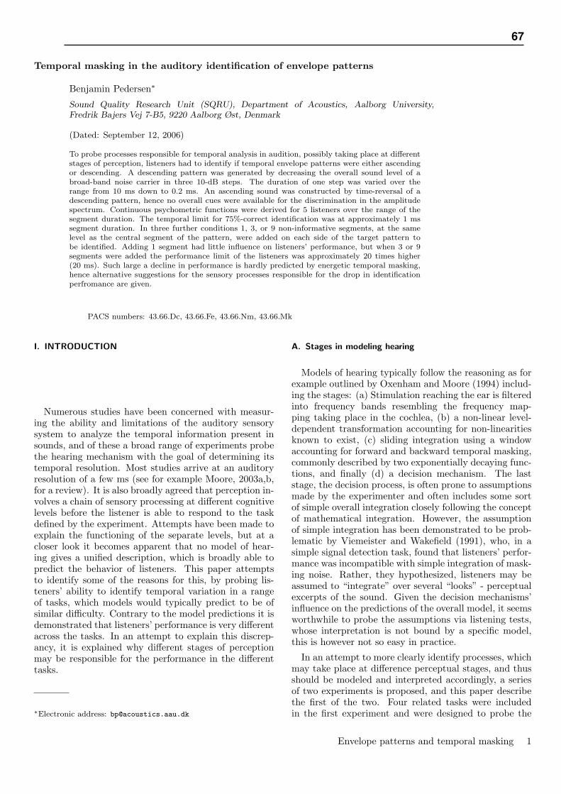
Temporal masking in the auditory identification of envelope patterns

Benjamin Pedersen∗



To probe processes responsible for temporal analysis in audition, possibly taking place at differentstages of perception, listeners had to identify if temporal envelope patterns were either ascendingor descending. A descending pattern was generated by decreasing the overall sound level of abroad-band noise carrier in three 10-dB steps. The duration of one step was varied over therange from 10 ms down to 0.2 ms. An ascending sound was constructed by time-reversal of adescending pattern, hence no overall cues were available for the discrimination in the amplitudespectrum. Continuous psychometric functions were derived for 5 listeners over the range of thesegment duration. The temporal limit for 75%-correct identification was at approximately 1 mssegment duration. In three further conditions 1, 3, or 9 non-informative segments, at the samelevel as the central segment of the pattern, were added on each side of the target pattern tobe identified. Adding 1 segment had little influence on listeners’ performance, but when 3 or 9segments were added the performance limit of the listeners was approximately 20 times higher(20 ms). Such large a decline in performance is hardly predicted by energetic temporal masking,hence alternative suggestions for the sensory processes responsible for the drop in identificationperfromance are given.

PACS numbers: 43.66.Dc, 43.66.Fe, 43.66.Nm, 43.66.Mk

I. INTRODUCTION

Numerous studies have been concerned with measur-ing the ability and limitations of the auditory sensorysystem to analyze the temporal information present insounds, and of these a broad range of experiments probethe hearing mechanism with the goal of determining itstemporal resolution. Most studies arrive at an auditoryresolution of a few ms (see for example Moore, 2003a,b,for a review). It is also broadly agreed that perception in-volves a chain of sensory processing at different cognitivelevels before the listener is able to respond to the taskdefined by the experiment. Attempts have been made toexplain the functioning of the separate levels, but at acloser look it becomes apparent that no model of hear-ing gives a unified description, which is broadly able topredict the behavior of listeners. This paper attemptsto identify some of the reasons for this, by probing lis-teners’ ability to identify temporal variation in a rangeof tasks, which models would typically predict to be ofsimilar difficulty. Contrary to the model predictions it isdemonstrated that listeners’ performance is very differentacross the tasks. In an attempt to explain this discrep-ancy, it is explained why different stages of perceptionmay be responsible for the performance in the differenttasks.

∗Electronic address: [email protected]

A. Stages in modeling hearing

Models of hearing typically follow the reasoning as forexample outlined by Oxenham and Moore (1994) includ-ing the stages: (a) Stimulation reaching the ear is filteredinto frequency bands resembling the frequency map-ping taking place in the cochlea, (b) a non-linear level-dependent transformation accounting for non-linearitiesknown to exist, (c) sliding integration using a windowaccounting for forward and backward temporal masking,commonly described by two exponentially decaying func-tions, and finally (d) a decision mechanism. The laststage, the decision process, is often prone to assumptionsmade by the experimenter and often includes some sortof simple overall integration closely following the conceptof mathematical integration. However, the assumptionof simple integration has been demonstrated to be prob-lematic by Viemeister and Wakefield (1991), who, in asimple signal detection task, found that listeners’ perfor-mance was incompatible with simple integration of mask-ing noise. Rather, they hypothesized, listeners may beassumed to “integrate” over several “looks” - perceptualexcerpts of the sound. Given the decision mechanisms’influence on the predictions of the overall model, it seemsworthwhile to probe the assumptions via listening tests,whose interpretation is not bound by a specific model,this is however not so easy in practice.

In an attempt to more clearly identify processes, whichmay take place at difference perceptual stages, and thusshould be modeled and interpreted accordingly, a seriesof two experiments is proposed, and this paper describethe first of the two. Four related tasks were includedin the first experiment and were designed to probe the

Envelope patterns and temporal masking 1

67

supposedly higher levels of perception in tasks of varyingdifficulty, but all putting similar demands on temporalresolution in the sensory system. The variation was madeby the addition of non-informative noise on the sides of a“target” pattern, which had to be identified (see Figure 1for an overview). Consequently, there will be a focus onvarious aspects of the higher level decision processes inthis paper while, in the second paper, it is demonstratedthat extremely low measures of temporal resolution ofhearing can be obtained by manipulating stimuli similarto the ones used in this work.

B. Neurophysiological and psychoacoustical evidence fordifferent stages in hearing

Naatanen and Winkler (1999) give an extensive reviewof the neurophysiological evidence that different stagesexist, and their findings are explained in somewhat dif-ferent terms than the model for example described byOxenham and Moore (1994). Naatanen and Winkler(1999) find evidence for and conclude that perception in-cludes the following stages (in this particular order): (a)Feature extraction, where specific features of the stimu-lation arise, and (b) a feature trace, i.e. the extractedfeatures are buffered for a while and remain availablefor (c) a unitary stimulus representation where differentfeatures are integrated and mapped onto a temporal di-mension. Of these stages the first two are consideredpre-representational and the last representational by theauthors, and only the last stage carries integrated infor-mation and information about temporal order. Also, theauditory information is only available for conscious per-ception after the last stage. However, it is clear thatspecific features may be available for conscious percep-tion before a fully integrated percept exists, for exam-ple the pitch of a level-fluctuating tone is available be-fore the temporal properties of the level-fluctuations arecompletely mapped to a temporal axis. Hence, it may behypothesized that there is a major difference in the per-formance of listeners in tasks where they can make judg-ments based on single static features alone or if they mustbe aware of the temporal properties of the stimulation inorder to do their task. In the discussion of listening ex-periments in which listeners can perform with a very finetemporal resolution it is often observed that the listenersperformed their task according to a difference in “qual-ity” between the stimuli defined by the task. This is forexample the case in the work described by Divenyi andHirsh (1974) where listeners were asked to judge the orderof three different tones in a sequence. The temporal sep-aration of the tones was varied making the discriminationtask increasingly difficult. This is interesting for the cur-rent discussion because the nature of the task seemed tochange with the temporal separation: When tones weresufficiently spaced the listeners had a clear impression ofa tonal sequence, this however changed when the separa-tion decreased, making it harder to identify the temporal

position of individual tones. Interestingly, for very shortseparations (in the order of a few ms), the listeners werestill able to perform the task, but based their judgmentssolely on the perceived quality of the entire sequence, notbeing able to identify individual tones.

This has inspired the current work, as this type oftask seems able to probe both perception of temporalorder and perception of features, taking place at rela-tively higher (e.g. decision device) and lower stages (e.g.temporal windowing) of cognition.

Further support for the notion of feature extractionmay be found in the psychoacoustic literature concerningauditory amplitude modulation detection (see Viemeisteret al., 2002, for a review). It is beyond the scope of thispaper to review this large body of literature, but it isinteresting to note how the concept of specialized modu-lation detectors (modulation detection filter banks) is in-troduced to explain the results of listening experiments.For the purpose of this paper, such detectors may wellbe considered specialized feature extractors. The notionof “hard-wired” modulation filter banks may be ques-tionable, but the evidence that a “modulation” featureis present in perception is interesting for the current dis-cussion.

Also, the literature concerning “feature extraction” inpitch perception and binaural hearing is interesting inthis context, and is reviewed more carefully by Pedersen(2006).

C. Probing “low” or “high” cognitive stages in listeningexperiments?

It is often assumed that listeners’ performance in rel-atively simple auditory tasks reflects peripheral stagesof hearing. It is however not obvious that this assump-tion is always valid. The question is for example raisedin a slightly different research area, namely in researchin reading and writing disabilities. The main questionis whether such disabilities may be caused by deficitsin the temporal processing and maybe even related toperipheral parts of the auditory sensory system. Re-views of the evidence are given by Farmer and Klein(1995) and Studdert-Kennedy and Mody (1995). Morerecently Schaffler et al. (2004) demonstrated that im-provements obtained by training people suffering fromdyslexia in “low-level” auditory tasks significantly trans-ferred to language related and phonological skills and tospelling. The auditory tasks used for training involvedfor example intensity, frequency discrimination, and gapdetection. In their framework such tasks were “low-level”per definition and it is not clear at which stages of per-ception the performance actually improved. It could rea-sonably be argued that the benefit of training would beassumed biggest at the higher levels of cognition, indi-cating that for example gap detection puts high demandon the higher levels of cognition. This would be at oddswith the way results of gap detection and for example


68 Paper 2

masking experiments are used to derive properties of atemporal window of auditory perception (as in Oxenhamand Moore, 1994, for example).

D. A task probing several levels of perception

The work described in this paper will put different de-mands on listeners’ ability to identify temporal propertiesvia a task which is, in its basic form, similar to the three-tone sequences used by Divenyi and Hirsh (1974). Butrather than changing frequency over the three elementsof a sequence (as Divenyi and Hirsh), the sequence iscomposed of three bursts of noise of different (ascendingor descending) overall level (Figure 1). In its basic formthere is a difference in quality between the ascending anddescending patterns. Later the difference in quality willbe diminished by the addition of non-informative noise onthe sides of the patterns. The listener thus has to identifythe relevant pattern embedded in the noise in order to doher/his task, thus putting demands on a different levelof perception. The use of level changes, as opposed tochanges in frequency, makes the task conceptually moresimilar to temporal masking and gap detection, possi-bly providing a bridge between the different classes ofexperiments. It will be explained and illustrated why atraditional “temporal window” model hardly predicts thedifference in performance in the relevant tasks.

According to a model based on “smoothing” by a tem-poral window it is expected that, in all tasks of the cur-rent experiment (different degrees of added noise), theperformance of the listeners declines at similar rate asthe duration of the stimulus segments is decreased, de-pending on the temporal extent of the “smoothing” win-dow. If this is not the case, however, that outcome sug-gests that different types of processing influence perfor-mance, possibly operating at different cognitive stagesacross the different tasks. The outcome will not explainhow to formulate a mathematical model of hearing, butit may provide important hints as to which aspects mustbe included and which concepts are incompatible withthe behavior of listeners.

II. METHOD

A. Listeners

Five listeners (3 female, 2 male, including the author(BP in the figures)) participated, and were recruited fromstudents at the university. The mean age of the partic-ipants was 24.6 years (range: 19 to 30 years). None ofthe listeners had a significant hearing loss (>20 dB HLat any of the frequencies 250, 500, 1k, 2k, 4k, 6k, 8kHz). Listeners BP and MC had previous experience inlistening tests, while LP, MK and DP participated in alistening experiment for the first time.

B. Apparatus

Sounds were generated on a computer and convertedat a sampling rate of 96 kHz and a resolution of 24 bit us-ing an external digital to analog converter (Edirol UA-5).A headphone amplifier (Tucker-Davis Technologies Sys-tem 3 HB7) was used for powering the headphones. Allsounds were presented diotically via headphones (SonyMDR v6). The listeners were positioned in a sound-insulated booth and gave responses via a custom-madebutton box with lights providing feedback.

C. Stimuli

The task of the listeners was to discriminate soundscontaining a descending pattern in the envelope fromsounds containing an ascending pattern. This was donein four different conditions as illustrated by the rows inFigure 1. The central part of the stimulus always con-tained the 3-segment long ascending/descending pattern,while the number of non-informative noise segments pre-ceding and succeeding the pattern was varied across con-ditions: In the 3-segment condition no noise segmentswere added, and in the 5-, 9-, and 21-segment conditions1, 3, and 9 non-informative noise segments were addedon each side of the target pattern. The segment durationwas the parameter that was varied by the psychophysicalprocedure. So for a given segment duration the overallduration of stimuli in different conditions was differentbecause the number of segments per sound was different.

1. Noise carrier

The patterns shown in Figure 1 represent schematicenvelopes of modulated noise carriers. The noise carrierwas the same type in all conditions, and it had a broad-band frequency spectrum, but not the properties of whitenoise.

Since the noise was used for probing temporal resolu-tion of the sensory system, a special carrier noise wasdesigned to avoid problems of inherent fluctuations ofthe noise carrier, which could be confused with fluctu-ations in the modulator amplitude. At short segmentdurations the amplitude of the modulated noise carriermust be able to change rapidly if it has to closely reflectthe envelope of the modulator. The carrier noise was de-signed fulfill both these requirements. Each sample inthe noise had a binary character, having a value of ei-ther A or −A, where A was given by the amplitude ofthe modulation envelope. The amount of negative andpositive samples was balanced within groups of two sam-ples, which means that all samples of the noise can bearranged in pairs of adjacent samples, always having op-posite sign for the amplitude A. This is illustrated inFigure 2. Within each pair of samples the order of Aand −A was random. As a consequence the amplitude of


69

1

7090

1

1 4

7090

1 4

1 4 7

7090

1 4 7

1 4 7 11 15 19

7090

1 4 7 11 15 19

Segment index

Am

plitu

de [d

B]

Figure 1. Stimuli used in different conditions: 3-, 5-, 9-, and21-segment conditions in each row respectively. The y-axisshows sound level for each segment. The x-axis shows thetemporal index of each segment, the actual duration of whichwas varied.

the modulated noise very closely followed the amplitudeof the modulator, because the mean of the squared sam-ple values of an excerpt will be very close to A2 for anygiven number of samples included in the excerpt, as longas the excerpt is more than one sample. Thus, for a run-ning mean applied to the modulated noise, the output ofthe running mean will reflect amplitude with a temporalresolution determined only by the extent of the windowused in the running mean.

For one track of trials the noise carrier was “frozen”.This was especially important for short segment dura-tions, where the perceived quality of a sound varies morebetween different noise carriers than between different di-rections of the target pattern. For short durations of thenoise carrier, its long term properties are not valid, mean-ing that the spectrum can change dramatically across dif-ferent short excerpts of the noise carrier. For each newtrack of trials a new “frozen” sequence of samples wasused.

A descending sound was generated by time-reversal ofthe corresponding ascending sound. Therefore the am-plitude spectra of the two sounds are identical over theduration of the sounds. It may be argued that the be-ginning of a sound is different in its fine-structure afterit has been time-reversed, which potentially provides acue for discrimination even if non-informative noise ispresent at the beginning. Therefore the noise carrier wasalways mirror-symmetric over the duration of a sound,with the line of symmetry in the middle of the centralsegment. For this reason non-informative segments in

Sample index

Sam

ple

valu

e

●

● ●

●

●

● ●

● ●

● ●

●

●

● ●

● ●

●

Figure 2. Example of a noise carrier excerpt. Blocks markedby gray and white background contain equally many negativeand positive samples in random order.

the 5-, 9- and 21-segment conditions are unaffected bytime-reversal of the stimuli, which was used to generatethe target patterns in opposite directions. Another con-sequence is that descending and ascending sounds startedand ended with the exact same samples within the threeconditions. Further, it makes the decomposition of thestimuli, as illustrated in Figure 14 in the appendix, pos-sible. The smallest possible segment duration is equalto the duration of 4 samples. To understand this, con-sider the central segment of a sound, which must obeythe following criteria: The segment has to contain equallymany positive and negative samples and at the same timebe mirror-symmetric, which cannot be fulfilled with lessthan four samples. In general the segment duration mustalways be a multiple of four samples.

A more thorough description of the statistical proper-ties of the stimuli is given in Appendix B.

2. Calibration

As shown in the Figure 1, the calibrated level of thenon-informative noise was always 80 dB SPL and the lev-els of segments of the target pattern were either 70, 80,90 dB SPL (ascending pattern) or 90, 80, 70 dB SPL (de-scending pattern). The setup was calibrated relative to asetup with the headphones positioned on a dummy-head(Kemar) where the level of a sine tone with a frequency of1 kHz was measured in the ear of the dummy-head. Also,the transfer function from the headphones to the ear wasrecorded. In this paper all sound pressure levels in dB re-fer to what would have been the level of a 1 kHz sine tone


70 Paper 2

at the applied gain settings. The actual sound pressurelevel at the ears will be lower, because the noise containsmore power at higher frequencies where the headphonetransfer function is highly attenuated. The actual soundlevel at the ears is estimated in Appendix C, where it isfound that the actual level at the ears is approximately13 dB lower than reflected by the calibrated levels.

D. Experimental procedure

A two-interval, forced-choice paradigm was adopted.In one trial the listener heard two sounds, one of whichcontained a descending pattern and the other containedan ascending one. The task of the listener was to iden-tify which sound contained the descending pattern. Theexperiment was divided into tracks in which trials con-tained only sounds from the same condition (see Figure1).

The use of an adaptive procedure was avoided to beable to detect non-monotonicities in the psychometricfunctions, and as to obtain “full” psychometric functionsas a function of the segment duration. Also, the perceivedquality of sounds of very different segment durations isdramatically different. Therefore it seemed natural togradually reduce the segment duration throughout onetrack in order to avoid a drop in performance becausethe listener had to change his/her decision criterion fromtrial to trial. However, it cannot be ruled out that effectsof this way of varying the segment duration is reflectedin the psychometric functions derived. Indeed it can beargued that the performance is worse in the beginningof each track because the listener has to become familiarwith the task. Thus the performance, as a function ofsegment duration, would be underestimated for long seg-ment durations, which always occurred in the beginningof a track. It could also be argued that the listener al-ways looses attention toward the end of a track, leadingto an underestimation of the performance as a functionof segment duration. Further it could be argued that theperformance is better for short segment duration becauseof long term learning effects. This is however unlikely, be-cause in the time frame of the entire experiment, differentsegment durations are almost perfectly balanced.

In one track the segment duration was slowly de-creased; in the 3- and 5-segment conditions from 10 ms to0.1 ms and in the 9- and 21-segment conditions from 100ms to 0.1 ms. The segment duration was reduced witha logarithmic step size with 80 steps per decade. Thusone 3- or 5-segment track contained 161 trials and a 9-or 21-segment track contained 241 trials.

E. Data collection

The presented results are based on 8 tracks per lis-tener per condition. So the total number of trials percondition per listener was 8 × 161 = 1288 in the 3- and

5-segment conditions and 8 × 241 = 1928 in the 9- and21-segment conditions. The listeners first went throughthe 3- and 9-segment conditions where tracks of bothconditions were presented in an alternating order. Onlythereafter the listener started the 5- and 21-segment con-ditions, also in an alternating order. All listeners wereinitially trained in the 3- and 9-segment conditions. Thesame segment durations were used in the training as inthe experiment proper, except for the very first tracksof trials in the 3-segment condition, which started witha segment duration of 100 ms. The amount of trainingrequired varied from 1 to 2 hours depending on the lis-tener. It was very different how easily listeners learnedthe task, especially in the 9-segment condition (the firstcondition with non-informative segments). No extensivetraining in the 5- and 21- segment conditions was given,because of the similarity to the 3- and 9-segment condi-tions. However a few initial tracks of trials in each of theconditions were used for familiarization before the datacollection started.

III. RESULTS

A. Procedure for deriving psychometric functions

For each listener, psychometric functions were derivedfor each of the 6 experimental conditions. These are dis-played in Figure 3. Figure 4 offers psychometric func-tions for pooled results across listeners. The psycho-metric functions were constructed in the following way:The results of all trials for a given listener and condi-tion, were sorted (according to the segment duration) andarranged in 50 overlapping bins. The bins were equallyspaced on a logarithmic time-axis, and the results of 200trials were included in each bin. This means that thecurves are considerably “smoothed” and only approxi-mately 3 estimates per decade are based on completelynon-overlapping data. Performance was estimated withineach bin by dividing the number of correct responses withthe total number of trials in that bin. By consideringeach trial a Bernoulli trial, 95%-confidence limits wereestimated based on the Binomial distribution. The 95%-confidence limits are marked as gray-shaded areas in thefigures.

Different number of trials were included in the binswhen the results were pooled across listeners (1000 trialsper bin).

Generally the psychometric functions show how listen-ers’ performance worsens as the segment duration be-comes smaller, which happens at relatively long segmentdurations when noise segments are added.

B. Procedure for estimating performance level

The segment durations corresponding to a performancelevel of 0.75 (75% correct responses) were estimated for


71

Condition Perf. level BP LP MK DP MC ALL3–segment 0.75 0.5 0.7 1.0 2.0 2.2 1.1

0.60 0.4 0.4 0.6 1.0 1.3 0.55–segment 0.75 0.3 0.8 0.6 14.4 2.4 1.1

0.60 0.1 0.2 0.3 1.5 0.8 0.29–segment 0.75 4.7 41.3 19.9 21.0 99.4 22.8

0.60 3.2 17.6 12.3 16.9 35.0 8.321–segment 0.75 9.5 22.6 29.8 27.9 – 30.0

0.60 5.7 13.0 25.4 16.8 – 11.7

Table I. Segment duration in ms at 0.75 and 0.60 performancelevels for all listeners in all conditions. The first row in eachcondition is the 0.75 limit and the second is the 0.60 per-formance limit. The last column, ALL, is derived from thepooled data for all listeners. The limit of MC in the 21-segment condition was outside the range of segment durationsused in the experiment.

all listeners in all conditions. That was done by fittingcurves to the obtained data and calculating the segmentduration where the fitted curve had an ordinate value of0.75. A logistic curve was used to model the psychometricfunctions, taking the following form:

Ψ(T ) =12

+12· ec(log(T )+k)

1 + ec(log(T )+k)(1)

Ψ models the probability of a correct response as afunction of the segment duration T . In the formula k de-termines the segment duration of the transition point ofthe psychometric function, and c determines the steep-ness of the fitted function at the transition. T is thesegment duration measured in seconds. The function isfitted on the logarithmic time axis by using log(T ) in theequation. As can be seen, when the segment durationapproaches 0, Ψ approaches 1/2 and when T approaches∞, Ψ approaches 1. That means the psychometric func-tion is forced to approach the chance level of 50% correctfor small segment durations, and for long segment du-rations it is forced to approach a performance level of100% correct. The coefficients c and k were estimated ina least square fit of Ψ to the binary response data. Thatis, Ψ is not directly fitted to the estimated and smoothedperformance curves (solid lines) in Figure 3 and 4.

C. Temporal limits for individual listeners

When considering the limits for temporal resolution es-timated in the different conditions as summarized in ta-ble I and illustrated in Figure 5 and 6, it is evident thatthere is a difference in performance between the 3- and9-segment condition, for which data were collected con-currently. When looking at actual values it is observedthat the limit in the 9-segment condition is 10 to 50 timeshigher than the limit in the 3-segment condition. Thisof course means than the duration of one segment in the

9-segment condition must be 10 to 50 times as long asin the 3-segment condition for the task to be of similardifficulty. A similar difference is observed when compar-ing the 5- and 21-segment conditions. Here the factoris in the range 2 to 50. If listener DP is excluded dueto the problematic estimate in the 5-segment condition(see Figure 5) the factor is in the range 30 to 50. Forthe pooled results of all listeners there is a difference of afactor 20 in the 3- and 9-segment conditions, and in the5- vs. 21-segment conditions the factor is approximately30.

1. Problematic estimates

In general the fitted curves follow the estimated psy-chometric functions quite well (see Figure 5). In some sit-uations, however, it is problematic to derive the 0.75 per-formance level: In the 21-segment condition listener MCnever performs significantly better than chance, hencea function cannot be fitted and no estimate of the per-formance limit given. In the 9-segment condition MC’sperformance may be underestimated as is also the casefor listener LP in that condition. In the 5-segment condi-tions the psychometric functions in general have a shal-low slope, which questions the validity of the estimatedlimit. For listener LP in the 5-segment condition, for ex-ample, a reasonable limit seems to be at 0.2 ms segmentduration (see Figure 5), however 0.8 ms was estimatedbased the fitted curve. From inspection of the curves itseems as if the knee-point where the psychometric func-tion reaches the level of chance is less variable across lis-teners than the point of the psychometric function whereperformance starts falling from “all correct”. Thus it canbe argued that a better estimate of the performance limitis obtained at a relatively small performance level; 0.60for example. For this reason estimated limits at this levelare also calculated and shown in table I.

D. Individual psychometric functions

An surprising phenomenon, not accounted for by thefitted curve, can be observed for listener MK in the 9-segment condition (see Figure 3). After the expecteddecline of the psychometric function it starts rising again,starting from a segment duration of approximately 2 msand peaking around 1 ms. Even below this segment du-ration MK’s performance stays significantly better thanchance. Before any of MK’s results were analyzed henoticed this effect himself and for the 9-segment condi-tion expressed that, in the beginning of the track of trialsthe task was easy, and soon got very difficult, but laterbecame easier again. The 95%-confidence limits in Fig-ure 3 show that this increase in performance at low seg-ment durations is significant. A similar effect, but muchweaker, can be observed for BP and LP: BP’s perfor-mance stays better that chance below 1 ms segment du-


72 Paper 2

Index

0

0.4

0.6

0.8

1.0

Index

0

Index

0

Index

0

Index

0

Index

0

0.1 1 10 100

Index

0

Index

0

0.1 1 10 100

Index

0

Index

0

0.1 1 10 100

0.4

0.6

0.8

1.0

Segment duration [ms]

Por

tion

of c

orre

ct r

espo

nses

BP3,9

LP3,9

MK3,9

DP3,9

MC3,9

BP5,21

LP5,21

MK5,21

DP5,21

MC5,21

Figure 3. Estimated psychometric functions for all listeners in all conditions. Segment duration on the x-axis and the proportionof correct responses on the y-axis. The upper row shows the results for the 3- and 9-segment conditions with the 3-segmentcondition more to the left. The lower row shows the 5- and 21-segment conditions where the 5-segment condition is more tothe left. The shaded areas illustrate the 95%-confidence limits.

Index

0

0.1 1 10 100

0.4

0.6

0.8

1.0

Index

0


Por

tion

of c

orre

ct r

espo

nses ALL

3,9ALL5,21

Figure 4. Same as Figure 3, but for the pooled data of alllisteners. The results of the 3- and 9-segment conditions arepresented in the left panel, and the results of the 5- and 21-segment conditions in the right.

ration, and there is a small increase in LP’s performanceat the same point where MK’s performance started in-creasing. However, the increase in performance is notsignificant for LP.

E. Comparing 3- with 5-segment condition and 9- with21-segment condition

When making these comparisons, caution should betaken, because the 3-segment condition was performed

before the 5-segment condition and the 9-segment be-fore the 21-segment condition. In terms of the temporallimit for discrimination, performance in the 5-segment issurprisingly similar to the 3-segment condition for mostlisteners. There are two possible reasons for this: (1) The3-segment condition was performed before the 5-segmentcondition, so training effects could be an explanation and(2) small amounts of added noise do not worsen the per-formance (some listeners actually performed better in the5-segment condition). In general the 21-segment condi-tion is harder for the listeners than the 9-segment con-dition, however, LP performs better in the 21-segmentcondition, but is the only exception, and further, whenthe relevant curves for LP are compared it is clear thatthe evidence for LP performing better in the 21-segmentcondition is very weak. Indeed, when the very begin-ning of the curves are not considered, the psychometricfunctions very closely follows each other in the two con-ditions.

IV. DISCUSSION

The addition of non-informative noise segments pre-and succeeding a target pattern dramatically impairedlisteners’ performance in discriminating ascending fromdescending target patterns. What are the perceptual rea-sons for this? The influence of the noise could be specu-lated to be of two different origins: (1) Energetic maskingor (2) informational masking (Durlach et al., 2003). Sincethe current task bears some resemblance with gap detec-


73

Index

0

0.4

0.6

0.8

1.0

Index

0

Index

0

Index

0

Index

0

Index

0

0.1 1 10 100

Index

0

Index

0

0.1 1 10 100

Index

0

Index

0

0.1 1 10 100

0.4

0.6

0.8

1.0


Por

tion

of c

orre

ct r

espo

nses

BP3,9BP3,9

LP3,9LP3,9

MK3,9MK3,9

DP3,9DP3,9

MC3,9MC3,9

BP5,21BP5,21

LP5,21LP5,21

MK5,21MK5,21

DP5,21DP5,21

MC5,21

Figure 5. Same data as presented in Figure 3, but also including the fitted curves for estimating the limits of performance(thick lines).

Index

0

0.1 1 10 100

0.4

0.6

0.8

1.0

Index

0


Por

tion

of c

orre

ct r

espo

nses ALL

3,9ALL5,21

Figure 6. Same as Figure 5, but for the pooled data of alllisteners. The results of the 3- and 9-segment conditions arepresented in the left panel, and the results of the 5- and 21-segment conditions in the right.

tion, it seems worthwhile to consider the former, whichis often used via a temporal window model (Oxenhamand Moore, 1994) to explain the performance of listen-ers in experiments where similar stimuli is used. As itwill be shown, a temporal window model does not read-ily explain the difference in performance in the differentconditions, so also the concept of informational mask-ing is worth deeper thoughts. The concept is very broadthough, and no formal model is readily available for test-ing the ideas.

A. Predictions of a temporal window model

The principle working of a temporal window model, isa temporal “smoothing” of the envelope of a given sound.This is achieved by convolving (sliding) a fixed window,whose width determines the temporal acuity, with theenvelope of the sound. In Appendix D the procedure isexplained more carefully, and Figure 10 to 13 give ex-amples of the output of the sliding window when it isapplied to the stimuli of the current experiment. Thefigures thus give some hints as to which cues can be usedfor the discrimination task. The top row of a given figurecontains descending stimuli and the bottom row ascend-ing. From left to right the segment duration is decreas-ing, and at the same horizontal position stimuli in thetwo rows are at the same segment duration. So, in termsof the experimental task, stimuli in the top row had tobe discriminated from that in the bottom (at the samehorizontal position).

From inspection of the figures is not clear why the dis-crimination of patterns in for example the 5-segment con-dition, should be much easier than in the 21-segment con-dition: Local peaks and dips might be hypothesized toprovide important cues, but these are more pronouncedin the 21-segment condition (compare for example Figure10 and 13 at T/τ = 1). Alternatively, skewness (or theslope of the envelope) may be thought to be importantfor the discrimination, but also in this case there is noindication that the addition of non-informative segmentmakes the envelope less skewed. What may be observedhowever, is that potential onset and offset cues are moredominant in the 3- and 5-segment conditions, and almostnon-existing in the 21-segment condition. This difference


74 Paper 2

is most prominent when the segment duration is rela-tively long compared to the time coefficient of the tempo-ral window. Compare for example the onsets and offsetsof the envelopes in Figure 11 and 13 at T/τ = 2. If onsetand offset cues are crucial for the discrimination it maybe observed that for example the 9-segment conditiongets easier when the segment duration gets so short thatthe “target pattern” begins to interfere with the onset.This explanation is intriguing since it makes it possibleto explain why listener MK was able to improve his per-formance for shorter segment durations in the 9-segmentcondition. The fact that MK was the only listener forwhom this effect was pronounced indicates that he wasmore sensitive to onset/offset cues. In the 5-segment con-dition it also appears that the “target pattern” interfereswith the onset to a large extent, which would explainwhy listeners performed surprisingly well in this condi-tion. It should be noted that temporal smoothing is nota prerequisite for the onset/offset hypothesis.

Interestingly, as it is shown in Appendix E, the ad-dition of non-informative noise has no influence on thedifference signal obtained when subtracting the descend-ing stimuli from the ascending. This is true both beforeand after the temporal smoothing, and may be an indi-cation that the temporal window model does not capturethe essential cognitive processes, which are heavily influ-enced by the added noise.

B. Comparison to temporal order judgments of tones

Divenyi and Hirsh (1974) already reported on a sim-ilar experiment where listeners had to judge the tem-poral order of tones. Their study included ascendingand descending (in frequency) 3-tone patterns, whose re-sults may be compared to the 3-segment condition of thepresent experiment. They found that well-trained listen-ers were able to identify the temporal patterns down toa limit of approximately 2 ms. This compares relativelywell to the limits found in this experiment for the 3-segment sequences, though also naive listeners were ableto perform the task at such a short segment duration.

C. Quality cues and temporal representation

In their review of neurophysiological experimentsNaatanen and Winkler (1999) establish the concepts ofpre-representational and representational forms of thepercept, where only in the representational form the per-cept has been mapped to a temporal dimension in per-ception. It seems worthwhile to interpret the results ofthe current experiment within this framework.

Auditory “features” of sound, which are already part ofthe percept at pre-representational stages, are fundamen-tal to their reasoning. They do not mention onset/offsetcues as specific features, but since it appears that theymay be important concepts in order to understand the

results of the present work, it is argued in the followingwhy they may reasonably be interpreted as “features”,which emerge already at a low level of perception.

1. Onsets and offsets as perceptual features

First, ecologically it makes good sense that onset andoffset transients are important “features” for the under-standing of the origin of a sound. Secondly, based ona review of neurophysiological and psychophysical ex-periments Phillips et al. (2002) conclude that the onsetof a sound has a particular elaborate representation inthe sensory system, especially within the first few ms ofthe sound. Interestingly this is consistent with MK’s in-creased performance in the 9-segment condition around1 ms, where the target pattern would enter the criticalonset time-frame. Thirdly, further evidence is for exam-ple given by Stellmack et al. (2005), who show how theauditory system is especially sensitive to level changesat the onset and offset of a sound. They showed this inan experiment where people were asked to detect levelincrements and decrements of a 5 ms probe at differentpositions in a sound with an overall duration of 50 ms.

If it is assumed that onsets and offsets are features or“qualities” of a sound, this means that they themselvesonly indirectly carry information of the fine details ofthe temporal structure, because only at later perceptualstages are features mapped to a temporal dimension. Forthe 21-segment condition it was illustrated (see Figure13) that there is almost no difference in onset and offsetcues for ascending vs. descending stimuli, which meansthat the listener cannot rely on qualitative differences tothe same extent as in the other tasks. Rather the listenermust single out the “target pattern”, which is only pos-sible when the percept has been mapped to the temporaldimension of perception at a relatively high level of cog-nition. Thus the results in this condition may indicatethe precision (“temporal resolution”) with which sound ismapped to the temporal dimension. Note that this typeof “temporal resolution” is most likely not in the senseof a sliding “temporal window”, but may be understoodusing concepts such as uncertainty, similarity, or atten-tion Durlach et al. (2003). If, on the other hand, there isa difference in quality (onsets/offsets) between ascendingand descending patterns, then the listener can discrim-inate based on features alone. If, as it was suggested,this is the case in the 3- and 5-segment conditions, thiswould explain the good performance of the listeners inthese conditions.

V. CONCLUSION

The addition of non-informative noise segments influ-enced the performance of listeners to an extent not read-ily predicted by a temporal window model. Rather, theinfluence could be better understood when different cog-


75

nitive stages of perception were assumed to influence theperformance in different conditions. If onset and off-set cues were considered “features” of the percept, thenNaatanen and Winkler (1999) provide a good frameworkfor understanding the results. The 21- and 9-segmentconditions required awareness of the temporal proper-ties of the patterns to a larger extent as did the 3- and5-segment conditions where listeners could rely on qual-itative onset/offset differences. The relatively poor per-formance in the 9- and 21-segment conditions may beunderstood in similar terms as informational masking(Durlach et al., 2003). In experiments involving infor-mational masking large individual differences in perfor-mance are often observed (Durlach et al., 2003), whichwas also the case in the present experiment.

A. Temporal masking and gap detection

Within the explanatory framework outlined in this pa-per, effects observed in temporal masking and gap detec-tion experiments, reflect the temporal limits of a given“feature”- or “quality”-extraction process. Thereforetemporal limits found in such experiments do not reflect“absolute” limits of the auditory processing. Since thenumber of decoded “qualities” are possible many, it can-not be ruled out that another “feature” may depend oneven finer temporal details of the sound. This, of course,can only be detected if a presented sound possesses therelevant “feature”. The accompanying paper (Pedersen,2006) demonstrates that a repeated version of the stimuliused in the present experiment can be discriminated atan extremely fine resolution, indicating the emergence ofa new “feature” via the repetition. A temporal windowmodel based on, in this context, relatively long time coef-ficient is at odds with the very fine resolution with whichlisteners can perform the discrimination of patterns.

If auditory features play an important role, as sug-gested by the present results, future research may beconcerned with identifying specific features, both via psy-choacoustical or physiological experiments. The criticalparameters for “feature” extraction need not only be oftemporal character, but could also be of spectral or of amore complex nature (e.g. modulation or informationalmasking). Stimuli may be varied across all of these di-mensions as to identify the critical range (temporal orspectral limits for example) for the operation of specific“feature extractors”.

VI. ACKNOWLEDGMENTS

The author would like to thank the people of Dr. NealViemeister’s research group at the Psychoacoustics Lab-oratory at the Department of Psychology, University ofMinnesota. The experiment presented in this paper wasperformed during a research visit at the laboratory. Theauthor is greatful for their valuable advice and feedback

●●●●●●●●●●●●●●●●●●●●●●●●●●●●●●●●●●●●●●●●●●●●●●●●●●●●●●●●●●●●●●●●●●●●●●●●●●●●●●●●●●●●●●●●●●●●●●●●●●●●●●●●●●●●●●

●●●

●●●●●

●●●●●

●●●●●●

●●●●●●●

●●●●●●●●

●●●●●●

●●●●●●

●●●●●●●●

●●●●●●●●●●

●●●●●●●●


Qua

ntiz

ed s

egm

ent d

urat

ion

[ms]

0.1 1 10

0.1

110

Figure 7. Quantized segment duration (y-axis) plottedagainst theoretic segment duration used in one track of trials.

and for providing most of the experimental equipment.

This research was carried out as part of the “Center-contract on Sound Quality” which establishes participa-tion in and funding of the “Sound Quality Research Unit”(SQRU) at Aalborg University. The participating com-panies are Bang & Olufsen, Bruel & Kjær, and DELTAAcoustics & Vibration. Further financial support comesfrom the Ministry for Science, Technology, and Develop-ment (VTU), and from the Danish Research Council forTechnology and Production (FTP).

Appendix A: QUANTIZATION OF SEGMENTDURATIONS

Because of discrete sampling in the signal generationand playback, actual segment durations of the stimuliplayed back was also discrete. That is, not all segmentdurations required in one track of trials could be realized.The procedure used to generate the noise carrier causedthe segment duration to be a multiple of four samples.The sampling rate used was 96 kHz, so for the very short-est segment durations the discretization becomes evident.This is illustrated in Figure 7, where the discrete segmentduration of all trials in one fixed track is plotted againstthe segment duration without discretization. All resultspresented in figures and in the table of this paper arebased on the segment durations of the stimuli the listen-ers heard, that is, the quantized durations.


76 Paper 2

Appendix B: SPECTRUM OF NOISE CARRIER

The amplitude spectrum of excerpts of the noise car-rier, as depicted in Figure 2 for example, is random. How-ever it is possible to derive the long term spectrum in asimilar way as it is possible to derive the spectrum ofwhite noise. The power spectrum can be calculated byFourier transform of the autocorrelation sequence of aninfinitely long noise sequence, when the mean of the noiseis zero (Oppenheim et al., 1999). So the first step is to de-rive the autocorrelation sequence, which for a sequence,x, of real numbers, is given by:

φxx[m] = E{xn+mxn} (B1)

Here E denotes the expectation value and φxx thevalue of the autocorrelation sequence at position m. Ifnow the positive and negative sample values depicted inFigure 2 are taken to be −A and A, then φxx can becalculated for different m. For arbitrary n, and m = 0,xn is either −A or A so:

φxx[0] = E{xnxn} = A2 (B2)

For m = 1 there are two possibilities: xn+1 and xn arein the same block (see Figure 2). If this is the case theirproduct is always −A · A = −A2. If they are not in thesame block, they are uncorrelated and the expectationvalue of their product is zero, because the product will beA·A, −A·(−A), A·(−A) and −A·A with equal frequency.In summary the expectation value will be −A2 for halfof the sequence and zero for the other half. This gives:

φxx[1] = E{xn+1xn} = −12A2 (B3)

The very same arguments can be used for m = −1 and:

φxx[−1] = E{xn−1xn} = −12A2 (B4)

For any other m, xn+m and xn will be in differentblocks and thus uncorrelated. Therefore the expectationvalue of their product is zero:

φxx[m] = E{xn−mxn} = 0 for m < −1 or m > 1(B5)

Now the power spectrum of the sequence x can befound by Fourier transform of φxx:

Frequency [Hz]

Pow

er d

ensi

ty [d

B]

1000 10000

−90

−80

−70

−60

−50

Figure 8. Power density spectrum of the noise carrier (seeFigure 2 and equation ).

Px(ω) ∝∞∑

m=−∞φxx[m]e−jωm

∝ (φxx[−1]ejω + φxx[0] + φxx[1]e−jω)

∝ −12A2(ejω + e−jω) + A2

∝ −12· 2A2 cos(ω) + A2

∝ A2(1− cos(ω))

Here Px is proportional to the power density spectrum,where the normalized frequency, ω, can be related to afrequency in Hz given the sampling rate used in the ex-periment (fs =96 kHz), via the Nyquist-Shannon sam-pling theorem and the relation ω = 2πf/fs. The RMSpower of the noise in the full frequency range is 1 forA = 1, because the noise samples are always −A or +A.The power density should be normalized, so the integralover the full frequency range is the overall RMS value,that is, the overall integral should equal 1 when A = 1.This is obtained in the following expression where f hasbeen substituted for ω and the single sided spectrum isobtained by a multiplication by 2:

Px(f) =2fs

A2(1− cos(2πf/fs) (B6)


77

Appendix C: SOUND LEVEL AT EAR

The transfer function from the headphones to the rightear of the dummy-head was measured, and the result isdepicted in Figure 9 as the dotted curve. It was cali-brated to have unity gain at 1 kHz (0 dB), but has beenoffset in the figure as to intersect the noise power densityspectrum (dashed curve) at 1 kHz. The solid curve isthe noise power density spectrum weighted by the trans-fer function to the ear. The noise spectrum is plottedfor the amplitude A = 1. Since the samples of the noisecarrier are either A or −A, the RMS value of the noisesequence is A2, which for A = 1 is 1 (= 0 dB). The RMSvalue of the noise can also be calculated by integratingthe noise power density spectrum over the relevant fre-quency range. In this way the RMS value of the weightednoise can be estimated by numerical integration. The re-sults of the numerical integration over the range 0.4 to 20kHz was 0.054 (= -13 dB). Below 0.4 kHz the noise hasonly insignificant power, and above 20 kHz the power ofthe weighted noise is also insignificant due to the attenu-ation of the headphone-to-ear transfer function (hearingis of course not very sensitive to frequencies above 20 kHzeither, but this has no influence on the RMS value). Insummary, at A = 1, the unweighted RMS was 0 dB, andweighting by the headphone-to-ear transfer function re-duced this to -13 dB. Consequently, 13 dB should be sub-tracted from the calibrated levels used throughout thispaper to account for the transfer function of the head-phones to the ear.

Appendix D: EXAMPLES OF OUTPUT OF SLIDINGWINDOW

In Figure 10 to 13 examples are given of the outputof a temporal window convolved with the envelope ofthe stimuli used in different conditions of the experimentand at different values of the segment duration. For adescription of the model see for example (Oxenham andMoore, 1994). The temporal window used in this paperis given by:

w(t) =

{Aet/τb t < 0Ae−t/τf t ≥ 0

The symbols τf and τb are time coefficients for for-ward and backward masking respectively. A symbolic de-scription of the window convolved with the stimuli of theexperiment was derived, and the results are graphicallyillustrated in the figures. Convolved stimuli is plottedas a function the segment duration divided by τ , whereτf = τ and τb = 2τ were chosen to illustrate the effectof asymmetry of the temporal window. The envelope ofthe stimuli before the temporal window is described bythe RMS sound pressure levels of the segments. As it isgenerally true in linear signal analysis the shape of theconvolved response reduces to the shape of the impulse

Frequency [Hz]

Pow

er d

ensi

ty [d

B]

500 1000 2000 5000 10000 20000

−80

−70

−60

−50

Figure 9. Weighted noise power density spectrum. The un-weighted noise spectrum (dotted line, as also depicted in Fig-ure 8) is weighted by the measured transfer function fromthe headphones to the right ear of the dummy-head (dashedcurve), which, in the figure, has been offset from unity gain(0 dB) at 1 kHz, as to intercept the noise spectrum at 1 kHz.The weighted power spectrum is the estimated power densityspectrum at the ear (solid curve).

response (here the temporal window) when the input sig-nal gets sufficiently short. Different shapes of the tempo-ral window have been proposed by other researchers (seePlack et al., 2002, for example), but since the analysis inthis chapter is based on visual inspection it only makessense to consider different temporal windows to the ex-tent that they look different. If they look very similar alsotheir output will look very similar. The variation in thetemporal window proposed by other researchers, will inmost cases not give rise to fundamentally different look-ing graphs of the output of the temporal window. It maybe argued that level compression in the sensory systeminfluences the process. The consequence of compressionis basically a change in the relative differences betweenthe three segment levels used to describe the envelopepatterns. On the output side of the temporal windowvery much the same compression can be observed, whichmeans that the same fluctuations exists in the output,but settles at different relative levels as compared to thenon-compressed case.

Appendix E: IDENTICAL DIFFERENCE BETWEENASCENDING AND DESCENDING PATTERNS ACROSS3-, 5-, 9-, AND 21-SEGMENT CONDITIONS

The convolution with a temporal window has themathematical property of being distributive, which


78 Paper 2

means that the difference between ascending and de-scending stimuli can be calculated in two ways: (1) Thetwo convolved signals for ascending and descending stim-uli can be subtracted or, (2) the ascending and descend-ing stimuli can be subtracted prior to convolution andafterward convolved with the temporal window. It ispossible to decomposed the used stimuli as illustrated inFigure 14. Using the stimuli components of the figure (xn

and xt), ascending stimuli (xascending) can be describedby:

xascending(t) = xn(−t) + xt(t) + xn(t)

And descending:

xdescending(t) = xn(−t) + xt(−t) + xn(t)

Subtracting the ascending and descending signals givesthe difference:

xascending(t)− xdescending(t) = xt(t)− xt(−t)

This shows that the difference between ascending anddescending stimuli is independent of the added noise(xn), both prior to or after convolution with a temporalwindow. The linear analysis is valid for all signals, whichcan be decomposed as illustrated in Figure 14. This istrue both when the envelope or the fine-structure of thesignals of the experiment are considered, and further it isalso valid in the case where a simple non-linear transform(as a function of signal level only) has been applied earlierin the process as to model compression for example.

Divenyi, P. L. and Hirsh, I. J. (1974). “Identification of tem-poral order in three-tone sequences.”, J. Acoust. Soc. Am.56, 144–151.

Durlach, N. I., Mason, C. R., Kidd, G., Arbogast, T. L., Col-burn, H. S., and Shinn-Cunningham, B. G. (2003). “Noteon informational masking.”, J. Acoust. Soc. Am. 113, 2984–2987.

Farmer, M. E. and Klein, R. M. (1995). “The evidence fora temporal processing deficit linked to dyslexia: A review”,Psychonomic bulletin & review 2, 460–493.

Moore, B. C. J. (2003a). An Introduction to the Psychologyof Hearing, 5th edition (Academic Press, San Diego, CA).

Moore, B. C. J. (2003b). “Temporal integration and contexteffects in hearing”, Journal of Phonetics 31, 563–574.

Naatanen, R. and Winkler, I. (1999). “The concept of au-ditory stimulus representation in cognitive neuroscience.”,Psychol. Bull. 125, 826–859.

Oppenheim, A. V., Schafer, R. W., and Buck, J. R. (1999).Discrete-time signal processing, 2nd edition (Prentice Hall,Englewood Cliffs, NJ).

Oxenham, A. J. and Moore, B. C. (1994). “Modeling the ad-ditivity of nonsimultaneous masking.”, Hear. Res. 80, 105–118.

Pedersen, B. (2006). “Discrimination of temporal patterns onthe basis of envelope and fine-structure cues”, in AuditoryTemporal Resolution and Integration: Stages of AnalyzingTime-Varying Sounds, 85–96 (Aalborg University).

Phillips, D. P., Hall, S. E., and Boehnke, S. E. (2002). “Cen-tral auditory onset responses, and temporal asymmetries inauditory perception.”, Hear. Res. 167, 192–205.

Plack, C. J., Oxenham, A. J., and Drga, V. (2002). “Linearand nonlinear processes in temporal masking”, Acust. ActaAcust. 88, 348–358.

Schaffler, T., Sonntag, J., Hartnegg, K., and Fischer, B.(2004). “The effect of practice on low-level auditory dis-crimination, phonological skills, and spelling in dyslexia.”,Dyslexia 10, 119–130.

Stellmack, M. A., Viemeister, N. F., and Byrne, A. J. (2005).“Comparing monaural and interaural temporal windows: ef-fects of a temporal fringe on sensitivity to intensity differ-ences.”, J. Acoust. Soc. Am. 118, 3218–3228.

Studdert-Kennedy, M. and Mody, M. (1995). “Auditory tem-poral perception deficits in the reading-impaired: A criticalreview of the evidence”, Psychonomic Bulletin & Review 2,508–514.

Viemeister, N. F., Rickert, M., Law, M., and Stellmack, M.(2002). “Psychophysical and physiological aspects of audi-tory temporal processing”, in Genetics and the Function ofthe Auditory System, Proceedings of the 19th Danavox Sym-posium, edited by L. Tranebjaerg, J. Christensen-Dalsgaard,T. Andersen, and T. Poulsen, 273–291 (Holmens Trykkeri,Denmark).



79

T τ = 4 T τ = 2 T τ = 1 T τ = 0.5

T τ = 4 T τ = 2 T τ = 1 T τ = 0.5

T τ = 0.25 T τ = 0.125 T τ = 0.0625 T τ = 0.03125

T τ = 0.25 T τ = 0.125 T τ = 0.0625 T τ = 0.03125

Time

Env

elop

e m

agni

tude

afte

r te

mpo

ral w

indo

w

Figure 10. Temporal window convolved with 3-segment stimulus envelope. Descending pattern in top row, and ascending inthe bottom row. From left to right the figure shows how decreasing the segment duration changes the output of the temporalwindow. The ratio of segment duration, T , to the time coefficient of the temporal window, τ , is indicated at the top of eachfigure. A different scaling of the y-axis is used in the two columns. x-axis shows time, scaled to accommodate all patternswithin the same frame.

T τ = 4 T τ = 2 T τ = 1 T τ = 0.5

T τ = 4 T τ = 2 T τ = 1 T τ = 0.5

T τ = 0.25 T τ = 0.125 T τ = 0.0625 T τ = 0.03125

T τ = 0.25 T τ = 0.125 T τ = 0.0625 T τ = 0.03125

Time

Env

elop

e m

agni

tude

afte

r te

mpo

ral w

indo

w

Figure 11. Same as Figure 10, but showing the temporal window convolved with 5-segment stimulus envelope.


80 Paper 2

T τ = 4 T τ = 2 T τ = 1 T τ = 0.5

T τ = 4 T τ = 2 T τ = 1 T τ = 0.5

T τ = 0.25 T τ = 0.125 T τ = 0.0625 T τ = 0.03125

T τ = 0.25 T τ = 0.125 T τ = 0.0625 T τ = 0.03125

Time

Env

elop

e m

agni

tude

afte

r te

mpo

ral w

indo

w


T τ = 4 T τ = 2 T τ = 1T τ = 0.5

T τ = 4 T τ = 2 T τ = 1T τ = 0.5

T τ = 0.25 T τ = 0.125 T τ = 0.0625T τ = 0.03125

T τ = 0.25 T τ = 0.125 T τ = 0.0625T τ = 0.03125

Time

Env

elop

e m

agni

tude

afte

r te

mpo

ral w

indo

w



81

xn(t)

Time

Time

Am

plitu

de

xn(t)

xt(t)

c(−5, 5)

c(0,

2)

Time

Am

plitu

de

xt(t)

Composite − Ascending pattern

c(−10, 10)

Time

Am

plitu

de

xt(t) xn(t)xn(− t)

Composite − Descending pattern

Time

Am

plitu

de

xt(− t) xn(t)xn(− t)

Figure 14. Decomposition of stimuli. All stimuli are based on the signal components xn and xt in the top row. Examples ofdescending and ascending patterns composed from xn and xt are shown in the two lower rows. The arrows which mark they-axes always intersect the time axis at t = 0.


82 Paper 2

Chapter 5

Paper 3:Discrimination of temporal patterns onthe basis of envelope and fine-structurecues

Discrimination of temporal patterns on the basis of envelope and fine-structure cues

Benjamin Pedersen∗



The importance of envelope vs. fine-structure cues was examined in tasks in which listeners hadto discriminate temporally ascending or descending envelope patterns. Decreasing the durationof the patterns made the tasks harder and continuous psychometric functions were obtained as afunction of the duration of a single pattern. In two further conditions, a fixed envelope patternwas repeated within a 0.75-s time window, so that, in one condition only the envelope of thepattern was repeated, and in the other, the fine-structure of a single pattern. The temporal limitat which ascending and descending patterns were still discriminable was found to be a durationin the range of 1 ms no matter whether only single patterns were presented or whether theenvelope of a pattern was repeated. Fundamentally different performance was observed when thefine-structure was repeated, in which case some listeners were able to discriminate patterns at thefinest temporal resolution that could be physically realized (20 µs). Further, noise was added priorto and succeeding the patterns to be identified, which severely degraded performance when theenvelope was repeated or if the pattern was not repeated. When fine-structure was repeated withadded noise, performance generally increased for the shortest durations of the pattern. The notionof “energetic masking” appears incompatible with this observation, but rather, the fine-structureseems to carry important cues for the discrimination.

I. INTRODUCTION

In an accompanying paper (Pedersen, 2006) it was dis-cussed how different stages of perception may be involvedin decoding the temporal information carried in sound.It was demonstrated how the addition of non-informativenoise segments influenced listeners’ performance in a taskwhere they were asked to identify ascending and de-scending patterns, to an extent not readily explainedby a temporal window model. In accordance with theframework set up by Naatanen and Winkler (1999) itwas suggested that pre-representational and representa-tional stages of perception might be the key in under-standing the results, the main reasoning being: At anearly pre-representational stage the sensory system de-tects “features” of sounds, which are only later, at therepresentational stage of perception, mapped to a tem-poral dimension. Only when the representational stageis reached are the features consciously available. For dif-ferent stimuli used in the previous experiment it variedto which extent stimuli could be identified by specificfeatures (onset/offset cues) or whether the auditory taskrequired temporal information about the envelope of thestimuli at a conscious level.

The main goal of the experiment described in thispaper, is to explore how stimuli with similar temporalproperties as that used in the earlier experiment may bemanipulated so “static” features, like pitch or timbre,emerge. Such features may depend on temporal detailsmuch finer than the temporal limits found in the previousexperiment.

∗Electronic address: [email protected]

A. Repeating pattern - importance of envelope andfine-structure

In the present experiment, the main idea was to letascending and descending 3- and 21-segment patternsrepeat themselves (see Figure 1 versus Figure 2). Intwo conditions (repetition of 3- and 21-segment patterns)fine-structure was preserved in each repetition and onlythe envelope of the pattern in two other conditions. Thisvariation was considered especially fit to probe severalideas introduced in the literature to understand percep-tion of time-variance. Viemeister and Wakefield (1991)hypothesized that listeners may integrate their percep-tion over multiple temporal looks. In this frameworkthe proposed stimuli potentially give insight into whethersuch looks are based on the envelope or the fine-structureof a sound. In the case of only the envelope being im-portant, identical performance would be expected fromthe listeners for the two types of repetitions (envelopeonly or fine-structure). Generally, identical performanceis predicted by any model, where only the envelope of asound is assumed to carry temporal information. In con-trast, if a difference in performance is observed, it canbe concluded that temporal information at a finer levelof detail than the envelope is represented in the sensorysystem. Such an outcome would be in conflict with forexample the temporal window model (see for exampleMoore, 2003).

B. Static features

The difference between the two versions of the repeat-ing stimuli (envelope only or fine-structure), in termsof perception, becomes most evident for high repetition

Discrimination on the basis of envelope and fine-structure 1

85

rates of the pattern, where the repetition of the fine-structure is clearly different in quality (pitch- or timbre-like features) from the repetition of envelope only. Thissuggests that static features may emerge, making thestimuli discriminable based on pre-representational tem-poral details.

C. Temporal processing in pitch and timbre perception

In the literature there has been some controversy as towhat extent pitch depends on the amplitude spectrumof a sound only, or if temporal coding plays a majorrole (see for example Moore, 2003, for a review). Thisis interesting in that it makes several suggestions fortemporal processing mechanisms in the sensory system,where both spectral and temporal pattern matching areinvolved, and is relevant for the interpretation of the re-sults of present experiment. In an experiment Patterson(1994a) presented repeating ramped and damped sinu-soids, which bears some resemblance with the conditionof the present experiment where the fine-structure of thepattern is repeated. He found that there is a clear dif-ference in the perceived quality depending on the direc-tion of the ramping, the ramped version having a muchstronger sinusoidal quality. Since ramped and dampedstimuli are spectrally identical, this demonstrates thattemporal processing plays an important role. Pattersondeveloped a model of the temporal processing, which hasmore recently been used by Krumbholz et al. (2005) inan attempt to predict listeners’ performance in an experi-ment where they had to detect regularity in a pulse train,and they found that temporal information was combinedacross frequency bands.

Using wide band-stimuli, the current experimentprobed hearing where supposedly different sensoryprocesses are crucial. This was done by varying the tem-poral extent of patterns over a wide time range. Themain goal was to determine whether auditory tempo-ral processing is restricted to analysis of the envelope ofsounds only. If this is the case, no difference in the per-formance of listeners was expected in tasks where fine-structure or envelope was repeated. Contrary to this,the results revealed that when the fine-structure was re-peated, the auditory system could rely on extremely finetemporal details, but not when only the envelope wasrepeated.

II. METHOD

A. Listeners

6 listeners participated in the experiment; 2 males and4 females with a mean age of 24.9 years (range: 21 to30). Prior to the experiment the listeners’ hearing wasscreened and nobody had significant hearing loss (> 15dB HL at more than one frequency at 0.25, 0.5, 0.75, 1,1.5, 2, 3, 4, 6, and 8 kHz). Except for the author (BP)

all listeners were students with little or no experience inlistening experiments.

B. Apparatus

A computer program controlling the experiment alsogenerated the stimuli. A sound card (RME HDSP9632)was used for digital to analog conversion at a sample rateof 192 kHz. The high sample rate made short temporalblocks possible. The converter had a resolution of 24 bitsthough only 7 different sample levels were used in the gen-erated digital signal (see Pedersen, 2006). A power am-plifier (Rotel RB-976MkII) modified to have a fixed gainwas used. The amplifier’s amplitude response coveredthe range from 2 Hz to 90 kHz. The sounds were pre-sented via headphones (Beyerdynamic DT990Pro). Thedata sheet of the headphones specified a frequency rangeof 5 Hz to 35 kHz, so the bandwidth of the headphonesdetermined the bandwidth of the full system.

The listeners were seated in a double-walled listeningcabin, and gave their responses via a custom made buttonbox with lights providing feedback.

C. Stimuli

The listening experiment contained 6 different condi-tions which will be referred to using the following ab-breviations, which are more thoroughly described in thenext two chapters:

• 3NO: 3-segment pattern with no repetitions

• 21NO: 21-segment pattern with no repetitions

• 3EN: 3-segment pattern with repetitions - the en-velope is repeating not the fine-structure

• 21EN: 21-segment pattern with repetitions - theenvelope is repeating not the fine-structure

• 3EX: 3-segment pattern with repetitions - the exactsame fine-structure of one pattern is repeating

• 21EX: 21-segment pattern with repetitions - the ex-act same fine-structure of one pattern is repeating

The task for the listener was always to discriminateascending from descending patterns. The forms of thebasic patterns without repetitions (NO conditions) areillustrated in Figure 1.

1. Noise carrier

A special designed noise carrier was modulated withthe envelope patterns of the different conditions. It had abroad-band characteristic, but not the properties of whitenoise. To allow for rapid level changes, it was designedwith several temporal constraints, which are thoroughly


86 Paper 3

explained by Pedersen (2006). Further, the noise carrierwas always mirror-symmetric within a single repetition,and was thus unaffected be time-reversal of the pattern,which was used to generate corresponding ascending anddescending patterns.

2. Repetitions of pattern

In the conditions where the pattern was repeating it-self, the form of one repetition was the same as in thenon-repeating case. In the repeating conditions, the pat-tern kept repeating within a fixed time frame of 0.75s. This is illustrated in Figure 2. As illustrated, thepattern was always repeated in a cycle with the dura-tion of 25 segments. This means that the repetition ratechanged when the segment duration changed. The 25-segment repetition cycle was used for patterns of both 3and 21 segments length. Especially in the EX conditionthe stimuli had a pronounced pitch for short segmentdurations. The fundamental frequency of the pitch isdetermined by the segment duration and the repetitioncycle, and thus repeated 3- and 21-segment patterns havethe same pitch at the same segment duration, because ofthe fixed 25-segment cycle. The total duration of onesound was not allowed to exceed the 0.75 s duration andno fractional patterns were allowed, so the duration ofthe sound was sometimes shorter than 0.75 s, most pro-nounced for the long segment durations. However, forthe very longest segment duration starting at 100 ms,a single repetition of 21 segments, exceeded the 0.75 stime-frame. Therefore the duration of a sound was al-lowed to exceed the 0.75 s limit in the case of only onesingle repetition of the pattern. Because of these con-straints, the 3-segment pattern only started repeating ata segment duration of 27 ms and the 21-segment patternat 16 ms, so above these segment durations all conditions,repeating and non-repeating, contained identical stimuli.

In the case of non-repeating stimuli it was shown byPedersen (2006) that across 3- and 21-segment condi-tions, the difference between ascending and descendingstimuli is identical (subtracting a descending 3-segmentpattern from a 3-segment ascending gives the same resultas subtracting a descending 21-segment pattern from a21-segment ascending. That is: The noise segments can-cels out and have no influence on the difference). Whenthere is no difference for the non-repeated patterns thereis of course no difference either when the patterns arerepeating. All possible cues for discrimination are con-tained in the difference signal, so mathematically the pos-sible cues for discrimination are independent of addednoise segments.

The difference between repeating the envelope (EN)and repeating fine-structure (EX) is illustrated in Figure3. The noise carrier has the same properties as in thenon-repeating conditions, which means that the carrieris mirror-symmetric within each repetition. Thereforethe entire sound is also mirror-symmetric in the EX con-

1

70

1

1 4 7 11 15 19

70

1 4 7 11 15 19

Segment index

Am

plitu

de [d

B]

Figure 1. Envelope of stimuli in the conditions without rep-etitions (NO conditions). Stimuli in the 3-segment conditionin the top row and stimuli in the 21-segment condition inthe bottom row. The two columns illustrate ascending anddescending patterns respectively.

dition, but not in the EN conditions (except when thesound contains only a single repetition). Hence ascend-ing and descending EN patterns do not have the exactsame spectrum, only within single repetitions.

3. Calibration

The setup was calibrated relative to a setup with theheadphones positioned on an artificial ear (Bruel & Kjær4153), with microphone (Bruel & Kjær 4134). The levelof a sine-tone with a frequency of 1 kHz was measuredin the artificial ear. In this paper all sound pressure lev-els in dB refer to what would have been the level of a1 kHz sine tone at the applied gain settings. The ac-tual sound pressure level at the ears will be lower, be-cause the noise contains more power at higher frequencieswhere the headphone transfer function is highly attenu-ated. Therefore the (unweighted) level of a continuousnoise carrier was also measured, and it was found to beapproximately 15 dB lower than the 1 kHz sine-tone atthe same gain settings of the system.

As shown in Figure 1 and Figure 2, the calibrated levelof the non-informative noise was always 70 dB SPL andthe level of segments of the target patter was either 60,70, 80 dB SPL (ascending pattern) or 80, 70, 60 dB SPL(descending pattern). These levels are lower (by 10 dB)than the levels used in the parallel study described byPedersen (2006). This was to reduce the annoying sensa-tion introduced by the multiple perceived onsets at longersegment durations in the conditions with repeating pat-tern.

D. Experimental procedure

In all conditions a three-interval, two-alternative forcedchoice paradigm was adopted. In one trial the listenerheard three sounds, of which either the second or thirdcontained a descending pattern and the two others con-


87

Index

0

1 4 7 10 14 18 22 26 30 34 38 42 46

7090

T25 segments

Index

0

Index

0

Segment index

Am

plitu

de [d

B]

Index

0

1 4 7 10 14 18 22 26 30 34 38 42 46

7090

T25 segments

Index

0

Index

0

Segment index

Am

plitu

de [d

B]

Index

0

1 4 7 10 14 18 22 26 30 34 38 42 46

7090

T25 segments

Index

0

Index

0

Segment index

Am

plitu

de [d

B]

Index

0

1 4 7 10 14 18 22 26 30 34 38 42 46

7090

T25 segments

Index

0

Index

0

Segment index

Am

plitu

de [d

B]

Figure 2. Envelopes of stimuli in the repeating pattern conditions (EN and EX). On the x-axis is the segment index and onthe y-axis the sound pressure level. The two top rows show the ascending and descending pattern in the 3-segment conditions,and the two bottom rows in the 21-segment conditions. Each row depicts one single sound where T is the fixed time frame forone sound having a value of 0.75 s. The patterns are always repeated in a 25-segment cycle.

Index

0

1 4 7 10 14 18 22 26 30 34 38 42 46

7090

Index

0

Index

0

Segment index

Am

plitu

de [d

B]

Index

0

1 4 7 10 14 18 22 26 30 34 38 42 46

7090

Index

0

Index

0

Segment index

Am

plitu

de [d

B]

Figure 3. Illustration of repeating envelope (EN) vs. repeating fine-structure (EX) in the top and bottom row respectively.Only ascending 21-segment stimuli are shown. The different shades of gray indicate that a different noise carrier is used foreach repetition. In the lower row the same shade of gray illustrates that the exact same noise carrier is used for each repetition.A sound with descending patterns is generated by mirroring each individual repetition, meaning that the order of “colors” fromleft to right is the same for de- and ascending stimuli.


88 Paper 3

tained an ascending one. The task of the listener was toidentify which sound contained the descending pattern,so the performance at chance level was correct identifi-cation in half of the trials.

The use of an adaptive procedure was avoided to beable to detect non-monotonicities in the psychometricfunctions, and as to obtain “full” psychometric functionsas a function of the segment duration. Also, the perceivedquality of sounds of very different segment durations isdramatically different. Therefore it seemed natural togradually reduce the segment duration throughout onetrack to avoid a drop in performance because the lis-tener had to change his/her decision criterion from trialto trial. However, it cannot be ruled out that an effectof this way of varying the segment duration is reflectedin the psychometric functions derived. Indeed it can beargued that the performance is worse in the beginningof each track because the listener has to become familiarwith the task. Thus the performance, as a function ofsegment duration, would be underestimated for long seg-ment durations, which always occurred in the beginningof a track. It could also be argued that the listener al-ways looses attention toward the end of a track, leadingto an underestimation of the performance as a functionof segment duration. Further it could be argued that theperformance is better for short segment duration becauseof long term learning effects. This is however unlikely, be-cause in the time frame of the entire experiment, differentsegment durations are almost perfectly balanced.

The experiment was divided into tracks in which trialscontained only sounds from the same condition. In onesuch track the segment duration was slowly decreased,starting from 100 ms and ending at 0.01 ms (conceptu-ally speaking only, since the smallest possible segmentduration was 0.02 ms due to the discrete sampling, seeAppendix A). The segment duration was reduced in log-arithmic steps with 40 steps per decade. Thus one trackcontained 161 trials.

In the NO conditions there was a silent period of 0.3s between the three sounds of one trial, and in the re-peating conditions the break was 0.1 s. In the NO con-dition a longer break was used, so the individual soundswere clearly separated also when the segment durationwas short and each sound was “click” like. A shorterbreak was used in the repeating condition, because theimpression from informal listening was that the shorterthe break the easier the task was. Making the break tooshort allows for interaction cues of the two sounds, butstill, 0.1 s is a long break compared to the temporal res-olution eventually achieved. Further, the impression ofthe author is that the cue which distinguished sounds forshort segment durations was a difference in the overall“quality” of the sounds, not a transition cue. However,the contrast of the difference in quality was more evidentfor shorter break periods.

E. Data collection

Data were collected in two phases. In the first phase 6tracks of trials were collected per condition, where tracksfrom different conditions were presented in a differentrandom order for each listener. After the completionof the first phase it was observed that the performancecurves were irregular for most listeners for short segmentdurations in the EX conditions. To examine the listeners’performance in this region, an additional 6 tracks werecollected in both conditions. The new data were collectedin the second phase in a similar way as in the first, butincluding only trials for short segment durations and inthe EX conditions only. In the second phase a track oftrials started at a segment duration of 1 ms, and, in onetrack, 80 trials were collected per decade.

In the first phase 6 × 161 = 966 trials were collectedin each condition, which gives 240 trials per decade toestimate each listener’s performance. In the second phasealso 966 trials were collected in each condition, but therange of the segment durations was halved, giving a totalof 480 trials per decade to estimate performance.

III. RESULTS

A. Procedure for deriving psychometric functions

For each listener, psychometric functions were derivedfor each of the 6 experimental conditions. These are dis-played in Figure 4. Figure 5 offers psychometric func-tions for pooled results across listeners. The psycho-metric functions were constructed in the following way:The results of all trials for a given listener and condi-tion, were sorted (according to the segment duration) andarranged in 150 overlapping bins. The bins were equallyspaced on a logarithmic time-axis, and the results of 100trials were included in each bin. This means that thecurves are considerably “smoothed” and only approxi-mately 2.4 estimates per decade are based on completelynon-overlapping data. Performance was estimated withineach bin by dividing the number of correct responses withthe total number of trials in that bin. By consideringeach trial a Bernoulli trial, 95%-confidence limits wereestimated based on the Binomial distribution. The 95%-confidence limits are marked as gray-shaded areas in thefigures.

Different number of trials were included in the binswhen the results were pooled across listeners (500 trialsper bin), and the number was also different for the curvesof results in the second phase (75 for individual data and500 for pooled data).

B. Procedure for estimating performance level

The segment durations corresponding to a performancelevel of 0.75 (75% correct responses) were estimated forall listeners in all conditions. That was done by fitting


89

Condition OH OS BP HT TM AU ALL3NO 2.12 1.69 0.47 2.30 2.17 9.06 2.2021NO 22.33 40.56 3.60 34.49 33.44 92.36 25.923EN 0.63 1.03 0.35 1.41 0.89 1.70 0.8821EN 25.80 35.65 2.62 24.50 36.88 118.71 26.243EX 0.25 0.48 0.11 0.31 0.29 1.04 0.3321EX 6.96 266.80 0.01 31.65 45.69 76.60 43.04

Table I. Segment duration in ms at 0.75 performance level forall listeners in all conditions. The last column, “ALL”, wasderived from the pooled data of all listeners.

curves to the data obtained in the first phase of the exper-iment and calculating the segment duration where the fit-ted curve had an ordinate value of 0.75. A logistic curvewas used to model the psychometric functions, taking thefollowing form:

Ψ(T ) =12

+12· ec(log(T )+k)

1 + ec(log(T )+k)(1)

Ψ models the probability of a correct response as afunction of the segment duration T . In the formula k de-termines the segment duration of the transition point ofthe psychometric function, and c determines the steep-ness of the fitted function at the transition. T is thesegment duration measured in seconds. The function isfitted on the logarithmic time axis by using log(T ) in theequation. As can be seen, when the segment durationapproaches 0, Ψ approaches 1/2 and when T approaches∞, Ψ approaches 1. That means the psychometric func-tion is forced to approach the chance level of 50% correctfor small segment durations, and for long segment du-rations it is forced to approach a performance level of100% correct. The coefficients c and k were estimated ina least square fit of Ψ to the binary response data. Thatis, Ψ is not directly fitted to the estimated and smoothedperformance curves (solid lines) in Figure 4 and 5.

C. Results of the first phase

The segment durations corresponding to a 0.75 perfor-mance level (75% correct responses) are summarized forall listeners in Table I: When comparing the 3-segmentconditions, it is evident that for all listeners the 75%-threshold is lowest in the 3EX (fine-structure repeated)condition followed by the 3EN (envelope repeated) andfinally the 3NO (no repetitions). So for the 3-segmentconditions there is a unequivocal rank order of the con-ditions. Such a pattern cannot be identified in the 21-segment conditions, the main reason being that the fit-ted curves provide a very poor fits to the listeners’ actualperformance in the 21EX condition, some of the derivedlimits are almost meaningless. Listener “BP” does in gen-eral have a lower limit than other listeners, which may

be explained by his greater experience in listening ex-periments. The difference in performance between “BP”and the other listeners seems to be more pronounced inthe 21-segment conditions than in the 3-segment condi-tions, indicating that experience more heavily influencesthe performance in the 21-segment conditions.

A closer look at Figure 4 allows for a more detailedcomparison of the listeners’ performance in different con-ditions: First it can be observed that performance is al-most identical across NO, EN and EX conditions for longsegment durations (above 20 ms). This was expected,since the tasks are identical across the mentioned con-dition before the pattern started repeating (segment du-ration ≥ 27 ms for 21-segment and 16 ms for 3-segmentpattern), except for the somewhat shorter period of si-lence between the three sounds of a single trial in theNO conditions. Considering all psychometric functions,going from long segment durations towards shorter dura-tions, performance starts to get worse at a certain pointand continuously becomes worse for a while. In mostcases performance continuously declines until it reachesthe chance level of 0.5, but this is not generally true. Forsome listeners in some conditions performance improvesagain for shorter segment durations. This is more pro-nounced in the EX conditions (in which the fine-structurerepeats), but it may also occur in other conditions, con-sider for example 21EN for listener “OH” or 3NO forlistener “OS” around segment duration of 0.06 ms. Theirregularities of the psychometric functions for shortersegment durations were examined in greater depth in thesecond phase of the experiment, but only for the EX con-ditions. The effects were considered too small in the otherconditions to deserve further study.

D. Results of the second phase

The results of the second phase of the experiment (fine-structure conditions only) are depicted in Figure 6 foreach individual listener and in Figure 7 offers poolingacross listeners. Only the range of segment durationsfrom 1 ms down to 0.02 ms was covered in the secondphase. No psychometric functions were fitted, becauseof the non-monotonicity of performance as a function ofsegment duration, which is evident from the figures.

1. Overall results of the second phase

First the overall effects can be considered by compar-ing Figure 5 and Figure 7. In the 3EX conditions theoverall performance of the listeners were almost identi-cal in the two phases, but what was only weakly evidentin the first phase is much clearer in the second phase,namely: There are two ranges of the segment durationwith “flat” performance (better than chance), the firstone starting from a segment duration of 1 ms down toabout 0.3 ms where performance is 0.85, and the second


90 Paper 3

Index

0

0.4

0.6

0.8

1.0

Index

0

Index0

Index

0

Index

0

Index

0

Index

0

Index

0

Index

0

Index0

Index

0

Index

0

0.4

0.6

0.8

1.0

Index

0

0.4

0.6

0.8

1.0

Index

0

Index

0

Index

0

Index0

Index

0Index

0

Index

0

Index

0

Index

0

Index

0

Index0

0.4

0.6

0.8

1.0

Index

0

0.4

0.6

0.8

1.0

Index

0

Index

0

Index

0

Index

0

Index

0

Index

0

0.01 1 10

Index

0

Index

0

0.01 1 10

Index

0

Index

0

0.01 1 10

Index

0

0.4

0.6

0.8

1.0


Por

tion

of c

orre

ct r

espo

nses

OH3NO

OH21NO

OH3EN

OH21EN

OH3EX

OH21EX

OS3NO

OS21NO

OS3EN

OS21EN

OS3EX

OS21EX

BP3NO

BP21NO

BP3EN

BP21EN

BP3EX

BP21EX

HT3NO

HT21NO

HT3EN

HT21EN

HT3EX

HT21EX

TM3NO

TM21NO

TM3EN

TM21EN

TM3EX

TM21EX

AU3NO

AU21NO

AU3EN

AU21EN

AU3EX

AU21EX

Figure 4. Estimated psychometric functions for all listeners in all conditions. Segment duration on the x-axis and the proportionof correct responses on the y-axis. The results of each listener are depicted in each column. Each row contains the results ofeach of the conditions: 3NO, 21NO, 3EN, 21EN, 3EX and 21EX from top to bottom respectively. The shaded areas illustratethe 95%-confidence limits. The dashed lines are the fitted curves used to estimate the 0.75 performance limits in Table I.

starting from 0.15 ms and down to 0.07 ms with a per-formance level of 0.65. Comparing the two phases, butfor the 21EX conditions, the overall performance may byslightly higher in the second phase. This indicates thatthere is only a modest training effect between the twophases. In both phases performance remains almost con-stant at a level of 0.7 for segment durations smaller than

1 ms. Note that performance at a given segment dura-tion is based on trials with the actual segment durationsin a narrower range in the second phase as in the first,which gives twice as high a resolution of the estimatedperformance curves.


91

Index

0

0.4

0.6

0.8

1.0

Index

0

Index

0

Index

0

0.4

0.6

0.8

1.0

Index

0

0.01 0.1 1 10 100

0.4

0.6

0.8

1.0

Index

0


Por

tion

of c

orre

ct r

espo

nses

ALL3NO

ALL21NO

ALL3EN

ALL21EN

ALL3EX

ALL21EX

Figure 5. Same as Figure 4, but with pooling of data acrosslisteners.

2. Individual results of the second phase

The individual performance curves (Figure 6) are muchharder to discuses in general terms. First, for most lis-teners, there is no significant deviation in performancein the second phase compared to the first. For some,however, performance is better in certain regions, consid-ering listener “HT” in the 3EX condition, for example,there is a peak in performance at a segment duration of0.1 ms, which is more pronounced in the second phaseof the experiment. There may be two reasons for this:(1) The resolution of the estimated performance curveis higher in the second phase, giving more pronouncedpeaks and dips, and (2) the listener has improved inperformance, which is easily understood in terms of theexperience gained throughout the experiment. Perfor-mance within each listener seems to decay and increaseat the same segment durations across the two phases ofthe experiment. Some listeners show strikingly similarbehavior, compare “HT” and “BP” in the 3EX condi-tions for example: Both have a “double” peak in per-formance centered at 0.1 ms segment duration. Thereis a weak indication that “TM” may also have one of

these peaks at 0.08 ms segment duration. All other lis-teners do not show signs of increasing performance afterthe first decline in the 3EX condition. A drop in perfor-mance between 0.2 and 0.15 ms segment duration seemsto be occur for all listeners. In the 21EX condition, mostlisteners show a peak in performance around a segmentduration of 0.1 ms. Before this increase in performancemost listeners have a dip, this is however not true for“OH” whose performance continually increases from 1 to0.1 ms segment duration, and even below 0.1 ms “OH”sperformance remains at a high level of approximately 0.8.Comparing 3- and 21-segment EX conditions in which thefine-structure is preserved, the same type of effects canbe observed; performance both increases and decreases invarious time-ranges: Where exactly this occurs, however,varies across the 3- and 21-segment conditions and alsovaries across listener. A good example of this is “OH”who, in the 3-segment conditions, performs increasinglyworse towards shorter segment durations, while the op-posite is the case in the 21-segment condition.

IV. DISCUSSION

The results showed that performance of the listenerswas fundamentally different when the fine-structure of apattern was repeated compared to the case where onlythe envelope of a single pattern was repeated. Whenonly repeating the envelope, only a modest improvementin performance compared to the non-repeating case couldbe observed (compare for example the psychometric func-tions for NO and EN conditions in Figure 5). Whenrepeating the fine-structure, performance was especiallydifferent in the 21-segment condition, where performanceremained significantly above the chance level over the fullrange of segment durations used in the experiment (seeFigure 5). Further, in the non-repeating and repeatingenvelope conditions, performance was always worse inthe 21-segments condition as compared to the 3-segmentconditions, which was not the case when fine-structurewas repeated. When analyzing the performance of thelisteners in the repeating fine-structure conditions in thesecond experimental phase, it was clear that individualpsychometric functions were strongly non-monotonic asa function of the segment duration (Figure 6).

A. Sensory stages of processing temporal information

To understand the present results, different perceptualprocesses are proposed as being responsible for the per-formance at different segment durations:

1. Segment duration above 25 ms: Listeners are awareof the pattern of level-fluctuations.

2. Segment duration above 1 ms: Listeners can dis-criminate patterns based on onset and offset cues.


92 Paper 3

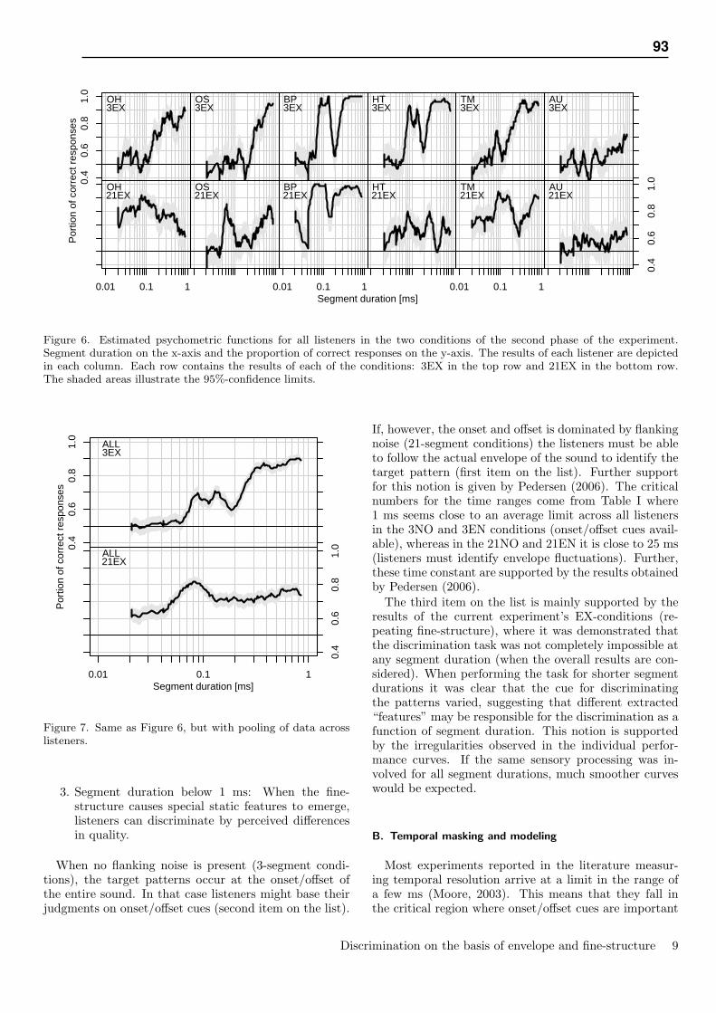
Index

0

0.4

0.6

0.8

1.0

Index

0

Index0

Index

0

Index

0

Index

0

Index

0

0.01 0.1 1

Index

0

Index

0

0.01 0.1 1

Index0

Index

0

0.01 0.1 1

Index

0

0.4

0.6

0.8

1.0


Por

tion

of c

orre

ct r

espo

nses

OH3EX

OH21EX

OS3EX

OS21EX

BP3EX

BP21EX

HT3EX

HT21EX

TM3EX

TM21EX

AU3EX

AU21EX

Figure 6. Estimated psychometric functions for all listeners in the two conditions of the second phase of the experiment.Segment duration on the x-axis and the proportion of correct responses on the y-axis. The results of each listener are depictedin each column. Each row contains the results of each of the conditions: 3EX in the top row and 21EX in the bottom row.The shaded areas illustrate the 95%-confidence limits.

Index

0

0.4

0.6

0.8

1.0

Index

0

0.01 0.1 1

0.4

0.6

0.8

1.0


Por

tion

of c

orre

ct r

espo

nses

ALL3EX

ALL21EX

Figure 7. Same as Figure 6, but with pooling of data acrosslisteners.

3. Segment duration below 1 ms: When the fine-structure causes special static features to emerge,listeners can discriminate by perceived differencesin quality.

When no flanking noise is present (3-segment condi-tions), the target patterns occur at the onset/offset ofthe entire sound. In that case listeners might base theirjudgments on onset/offset cues (second item on the list).

If, however, the onset and offset is dominated by flankingnoise (21-segment conditions) the listeners must be ableto follow the actual envelope of the sound to identify thetarget pattern (first item on the list). Further supportfor this notion is given by Pedersen (2006). The criticalnumbers for the time ranges come from Table I where1 ms seems close to an average limit across all listenersin the 3NO and 3EN conditions (onset/offset cues avail-able), whereas in the 21NO and 21EN it is close to 25 ms(listeners must identify envelope fluctuations). Further,these time constant are supported by the results obtainedby Pedersen (2006).

The third item on the list is mainly supported by theresults of the current experiment’s EX-conditions (re-peating fine-structure), where it was demonstrated thatthe discrimination task was not completely impossible atany segment duration (when the overall results are con-sidered). When performing the task for shorter segmentdurations it was clear that the cue for discriminatingthe patterns varied, suggesting that different extracted“features” may be responsible for the discrimination as afunction of segment duration. This notion is supportedby the irregularities observed in the individual perfor-mance curves. If the same sensory processing was in-volved for all segment durations, much smoother curveswould be expected.

B. Temporal masking and modeling

Most experiments reported in the literature measur-ing temporal resolution arrive at a limit in the range ofa few ms (Moore, 2003). This means that they fall inthe critical region where onset/offset cues are important


93

according to the reasoning outlined above. A reinterpre-tation of for example gap detection experiments whereno “smoothing” process is assumed, could take the fol-lowing form: Traditionally, a sliding temporal windowis thought to account for the masking, and is for exam-ple fitted by Oxenham and Moore (1994) giving differenttime coefficients for pre and post masking. These timecoefficients might be a measure of the width of a timewindow within which onsets and offsets are decoded, Or,to put it in other words, the auditory system “sees” thetemporal variation through a temporally limited window.Relatively long and short post and pre masking respec-tively is normally found, which translates into a relativelylong window for analyzing offsets and short window foronsets. That is, the “temporal window” is not responsi-ble for smoothing, but decisive in determining when anevent is considered a new onset. Ecologically this makesgood sense since sounds are most often characterized be arelatively abrupt (short window) onset and slow (longerwindow) decay.

The results of the repeated fine-structure (EX) condi-tions are clearly at odds with models including a slidingtemporal window, supported in two ways: (1) The dis-crimination task was possible at a resolution far betterthat what is normally predicted (observed in the order of60 µs as compared to 2 ms, which is in the typical rangeof a temporal window), and (2) a temporal window givesa smooth decline in performance (as a function of theextent of temporal details, which in this case is givenby the segment duration), which is inconsistent with theobserved discontinuities in the performance curves. Sur-prisingly the 21EX (21-segment, repeated fine-structure)condition was generally easier for very short segment du-rations than 3EX (3-segment, repeated fine-structure).This argues against any “power” or “energy” masking.Rather, because the difference between ascending anddescending patterns is identical across 3- and 21-segmentconditions, as argued by Pedersen (2006), relative phasedifferences may be important properties.

Ideas introduced to understand pitch perception (seefor example Moore, 2003) may be helpful to a deeper un-derstanding. Both spectral and temporal pattern match-ing have been suggested to play a role in pitch perception,and support for both ideas has been found. Sounds in therepeated fine-structure (EX) conditions had a clear pitchquality for short segment durations, but identical spectra.So temporal properties are crucial for the discriminationand may be reflected in pitch, but also different conceptsmay be of importance, as for example timbre, and cuesnormally used for spatial localization.

Patterson (1994b) applied a model utilizing temporalproperties to explain the difference in perceived qualityof ramped and damped sinusoids, but argues that thetemporal information may not be preserved with a finerresolution than 1 ms, which is significantly worse that thelimit suggested by the result of the current experiment,and thus the model seems incompatible with the stimuliof the present experiment.

C. Monaural and binaural phase sensitivity

Very different measures of the auditory ability to de-tect phase differences are obtained in studies using bin-aural or monaural stimuli. In the monaural case, thefinest temporal resolution measured is in the range of 0.2ms as found by Henning and Gaskell (1981), who usedRonken’s paradigm (Ronken, 1970), in which the delaybetween two clicks of different levels is varied. The taskof the listener is to detect the order of the clicks (high-lowor low-high level). Time-reversal is used to change theorder of the levels so no spectral cues are available. Theshortest delay between pulses at which the patterns canbe discriminated is thus a measure of temporal resolu-tion. If the task of the listener is to discriminate temporaldisparities across the ears using binaural stimuli, muchshorter temporal limits have been found (in the order ofsome µs). For example Klumpp and Eady (1956) foundthat listeners could discriminate stimuli where the inter-aural time differences was in the order of 9 µs. This vastdiscrepancy in temporal resolution found in binaural inmonaural listening tests has lead to the suggestion thatbinaural processing (as for example cross-correlation ofthe stimulation of the two ears) is responsible for the finetemporal resolution in the binaural case. But it couldreasonably be argued that the binaural processing has totake place on the basis of the monaural input from eachear. Hence, monaural temporal resolution should be atleast as good as that of the binaural system. The dis-crimination between temporal resolution in binaural andmonaural hearing is mostly motivated by the fact that nolistening experiment using monaural stimuli has demon-strated temporal resolution in a comparable range to re-sults of binaural experiments. Interestingly the presentexperiment demonstrated very fine temporal resolutionin a monaural task (EX conditions), where some listenerswere still able to perform temporal discrimination whenthe segment duration was as low as 20 µs. This value iscomparable to temporal limits found in binaural listeningtests. This leads to the suggestion that there is no reasonfor making a sharp division between the sensory systemworking in a “binaural” or a “monaural” mode. Thusthe different critical time regions found in the presentexperiment may be compared to effects known to existin binaural hearing: It was suggested that in the criticaltime-region above 1 ms, onset and offset played an im-portant role. Interestingly, in term of the critical timerange, this coincides with the “precedence effect” in bin-aural hearing (Blauert, 1999), where 1 ms has been foundto be the critical lower limit for the precedence effect tooccur. The upper limit is in the range 5 to 50 ms. Eco-logically it makes good sense that the precedence effectis tightly connected to the decoding of onsets, and to asmaller extent, offsets. Another effect found in binau-ral experiments is that listeners’ ability to follow spa-tial movements of a sound source seems to be limited toa certain speed of movement. This effect has been de-scribed as “binaural sluggishness”, and Blauert (1972)


94 Paper 3

suggests that fluctuations in location at a rate of ap-proximate 2.5 Hz may be followed well. This coincides,to some extent, with the suggested limit of this paperwhere listeners must be able to follow the level fluctua-tions to perform the discrimination task (25 ms). Theidentification of similar critical time-ranges in both bin-aural and monaural listening, may lead to the conclu-sion that they are based on the same processes. Often,models utilizing cross-correlation are used to explain theperformance in binaural tasks. This may however seemincompatible with the notion of fundamental “feature ex-traction” processes at the lowest peripheral levels as ex-plained by Naatanen and Winkler (1999). A full trace ofthe fluctuations of the sound is required to perform cross-correlation, and a full trace may not be available if thepercept has been encoded as different features. Ratherit may be hypothesized that the binaural system utilizesthe extracted features to determine the spatial locationof a given sound source. As was demonstrated by Pat-terson (1994b), the perceived pitch of a sound dependson temporal details, so for example pitch-like cues mightbe compared across the two ears and would reflect differ-ences in temporal details of the sound across the ears.

V. CONCLUSION

The presented results suggest that fine-structure playan important role in auditory temporal processing, whichis evident from the observation that listeners alwaysperformed better in conditions where the fine-structurewas repeated compared to the case of only the enve-lope being repeated. For short segment durations, lis-teners showed remarkably good performance when non-informative noise segments were added and fine-structurewas repeated (21EX condition). No lower limit for thesegment duration at which listeners could perform thetask was observed in this condition even though patternswere presented at segment durations as low as 20 µs. Thisis hard to reconcile with the notion of energetic mask-ing, which one would assume to cause performance tobe generally worse in conditions where non-informativenose is present. Further, it seems to contradict the no-tion of “smoothing” of the envelope at peripheral stagesof temporal processing in the auditory system. Sincea similarly good performance was not observed in theconditions where only the envelope was repeated, thismay suggest that fine-structure cues have to be “static”(steady-state) to some degree, as the stimuli of the re-peated envelope conditions in principle contain a wealthof fine-structure cues. This supports the notion of the ex-traction of “static” features relying on very fine temporalcues.

A. Topics for further inquiry

Future experiments may try to more specifically iden-tify “features” and which properties, spectral and tempo-ral, are crucial for their perception. Temporal patternsmay also be frequency filtered to examine how temporalinformation is combined across critical frequency bands,possibly showing different effects in the different criticaltime regions. Hopefully such experiments would lead to abetter understanding of different sensory factors respon-sible for decoding the temporal properties of sound.

VI. ACKNOWLEDGMENTS

This research was carried out as part of the “Center-contract on Sound Quality” which establishes participa-tion in and funding of the “Sound Quality Research Unit”(SQRU) at Aalborg University. The participating com-panies are Bang & Olufsen, Bruel & Kjær, and DELTAAcoustics & Vibration. Further financial support comesfrom the Ministry for Science, Technology, and Develop-ment (VTU), and from the Danish Research Council forTechnology and Production (FTP).

Appendix A: QUANTIZATION OF SEGMENTDURATIONS

Because of discrete sampling in the generation andplayback, actual segment durations of the stimuli playedback was also discrete. That is, not all segment durationsrequired in one track can be realized. The procedure usedto generate the noise carrier caused the segment durationto be a multiple of four samples. The used sampling ratewas 192 kHz, so for the very shortest segment durationsthe discretization becomes evident. This is illustrated inFigure 8 where discrete segment duration of all trials inone fixed track is plotted against the segment durationwith no discretization. All results presented in figuresand in table in the paper are based on the segment du-rations of the stimuli the listeners heard, that is, thequantized durations.

Appendix B: SPECTRUM OF NOISE CARRIER

The amplitude spectrum of the non-modulated and in-finitely long noise carrier has broad-band character, butis not similar to white-noise. Rather, it has relativelylow power contained at low frequencies and high powerat higher frequencies as shown in Figure 9. The noisecarrier is described in greater detail by Pedersen (2006),who also describes a procedure for deriving the amplitudespectrum.


95

●●●●●●●●●●●●●●●●●●●●●●●●●●●●●●●●●●●●●●●●●●●●●●●●●●●●●●●●●●●●●●●●●●●●●

●●●●●●●●●●●●●

●●●●

●●●●

●●●●●●

●●●●

●●●●●

●●●●●●●

●●●●●●●●●●●●

●●●●●●●●●●●●●


Qua

ntiz

ed s

egm

ent d

urat

ion

[ms]

0.01 0.1 1 10

0.01

0.1

110

Figure 8. Quantized segment duration (y-axis) plottedagainst theoretic segment duration used in one track of trials.

Frequency [Hz]

Pow

er d

ensi

ty [d

B]

1000 10000 100000

−90

−80

−70

−60

−50

Figure 9. Amplitude spectrum of the noise carrier (see Ped-ersen, 2006, for its definition).

Blauert, J. (1972). “On the lag of lateralization caused by in-teraural time and intensity differences”, Audiology 11, 265–270.

Blauert, J. (1999). Spatial hearing: The psychophysics of hu-man sound localization, 2nd edition (Cambridge, Mass, MITPress).

Henning, G. B. and Gaskell, H. (1981). “Monaural phasesensitivity with Ronken’s paradigm”, J. Acoust. Soc. Am.

70, 1669–1673.

Klumpp, R. G. and Eady, H. R. (1956). “Some measure-ments of interaural time difference thresholds”, J. Acoust.Soc. Am. 28, 859–860.

Krumbholz, K., Bleeck, S., Patterson, R. D., Senokozlieva,M., Seither-Preisler, A., and Lutkenhoner, B. (2005). “Theeffect of cross-channel synchrony on the perception of tem-poral regularity.”, J. Acoust. Soc. Am. 118, 946–954.

Moore, B. C. J. (2003). An Introduction to the Psychology ofHearing, 5th edition (Academic Press, San Diego, CA).

Naatanen, R. and Winkler, I. (1999). “The concept of au-ditory stimulus representation in cognitive neuroscience.”,Psychol. Bull. 125, 826–859.

Oxenham, A. J. and Moore, B. C. (1994). “Modeling the ad-ditivity of nonsimultaneous masking.”, Hear. Res. 80, 105–118.

Patterson, R. D. (1994a). “The sound of a sinusoid: Spectralmodels”, J. Acoust. Soc. Am. 96, 1409–1418.

Patterson, R. D. (1994b). “The sound of a sinusoid: Time-interval models”, J. Acoust. Soc. Am. 96, 1419–1428.

Pedersen, B. (2006). “Temporal masking in the auditoryidentification of envelope patterns”, in Auditory Tempo-ral Resolution and Integration: Stages of Analyzing Time-Varying Sounds, 67–82 (Aalborg University).

Ronken, D. A. (1970). “Monaural detection of a phase dif-ference between clicks”, J. Acoust. Soc. Am. 47, 1091–&.



96 Paper 3

Appendix A

Loudness models: Specifications andevaluations

A.1 Specification of models for prediction of loudness judg-ments

This appendix accompanies Section 3.5, where a broad range of models are fitted to listeners’ judg-ments of loudness. The appendix contains the mathematical specification of each of the 15 modelsapplied. Each specification gives the formulation of the model of perceived loudness (L) as a functionof the ten segment levels (vector x, and xi where i is the segment index). In Section 3.5 the actualprocedure for fitting the models to the listeners’ responses is given.

A short name and number identify each model in its headline, where also the number of parametersis given, which specify the number of parameters which are estimated in the fitting procedure. It maybe noted that this number is alway larger than the number of parameters which occurs in the expressionfor L by one. The “extra” parameter is the threshold criterion, c, as it appears in Equation 3.3.

Further characteristics of each model are given in five fields: “Formula”, “model coefficients”,“special case of”, “extends” and “short description”. The “formula” field gives the mathematical equa-tion for L. The “model coefficients” field shortly describes the functioning of the model parameters.The “special case of” field is a list of models, which are more general formulations of the relevantmodel. That is, by fixing some of the parameters in the more general models, they become identical tothe relevant model. “Extends” is a list of models for which the opposite is the case, that is, by fixingparameters of the relevant model it becomes identical to the simpler models. The “short description”field gives a short description of the main ideas and purpose of the model.

If it is not straightforward, it is explained in the “extends” field how the parameters of the modelshould be fixed to give identical predictions to the listed “extends” models.

98 Loudness models: Specifications and evaluations

M1 Mean 2 parameters

Formula:L(x) = wmean(x)

Model coefficients:w is a weighting coefficient indicating the sensitivity to changes in the meanof x.

Special case of:

M6, M7, M8, M9, M10, M11, M12, M13, M14, M15

Short description:Listener judgment is predicted from a simple mean value of the 10 segmentlevels.

M2 Maximum 2 parameters

Formula:L(x) = wmax(x)

Model coefficients:w is a weighting coefficient indicating the sensitivity to changes in the max-imum of x.

Special case of:

M7, M11, M12, M13

Short description:

Listener judgment is predicted from the maximum of the 10 segment levels.

M3 Minimum 2 parameters

Formula:L(x) = wmin(x)

Model coefficients:w is a weighting coefficient indicating the sensitivity to changes in the min-imum of x.

Special case of:

M7, M11, M12, M13

Short description:

Listener judgment is predicted from the minimum of the 10 segment levels.

Specification of models for prediction of loudness judgments 99

M4 Variance 2 parameters

Formula:

L(x) = wvar(x) =w9

10

∑i=1

(xi−mean(x))2

Model coefficients:w is a weighting coefficient indicating the sensitivity to changes in the vari-ance of x.

Short description:

Listener judgment is predicted from the variance of the 10 segment levels.

M5 Envelope profile 3 parameters

Formula:L(x) = wsl pα +wintβ

Model coefficients:A linear regression fit to the segment levels as a function of segment in-dex determines the slope, α , and intercept, β , of the regression line. Theregression coefficients are linearly weighted by wsl p and wint respectively.

Extends:M1

The intercept, β , can be calculated as: β = mean(x)− αmean(segidx),where segidx is the segment index from 1 to 10, therefore: mean(x) =β +αmean(segidx). Thus, if wsl p = 1 and wint = mean(segidx) = 5.5, themodel gives same predictions as the “mean” model if the two coefficientsare further scaled by w from model M1. This proves that M1 is a specialcase of M5.

Short description:For a given sound a line is fitted to the levels of the ten segments, withsegment index as the x-value and segment level as the y-value. A leastsquare fit gives the parameters α (slope) and β (intercept) for the best fittingline. Negative value for α thus indicates that the sound is descending fromthe beginning toward the end of the sound and positive value indicates anascending temporal profile of the sound. The listeners behavior is modeledas the slope weighted by a factor wsl p and the intercept by wint .


M6 Polynomial non-linearity 3 parameters

Formula:

L(x) =10

∑i=1

wsqx2i +wlinxi

Model coefficients:A quadratic term of the segment levels is scaled by wsq, and linear term bywlin.

Special case of:

M10, M15

Extends:

M1

Short description:Extends the mean model (M1) and introduces a quadratic term of the seg-ment levels. The sum of the segment levels is scaled by the factor wlin andthe sum of the squared levels by wsq.


M7 Attention weighting 3 parameters

Formula:

L(x) = w10

∑i=1

xpi

∑10j=1 xp

jxi = w

∑10i=1 xp+1

i

∑10i=1 xp

i

Model coefficients:w is a weighting coefficient indicating the sensitivity to changes in the atten-tion weighted sum of x. p is an exponent determining how strongly attentionis guided toward more salient segments in term of their relative level withina sound.

Special case of:

M11, M12, M13

Extends:M1, M2, M3

With p = 0, the attention weight (in front of xi in the central expres-sion) becomes 0.1, which makes the model identical to M1. With papproaching ∞, the attention weight will approach 1 for the maximumsegment, and 0 for the others. With p approaching−∞, the attention weightwill approach 1 for the minimum segment, and 0 for the others. ThereforeM2 and M3 are also special cases of M7.

Short description:This model weights each segment level by its own level in relation to all 10segments of the sound. The relative weight for the i’th segment is given by:

xpi

∑10j=1 xp

j.


M8 Moment of inertia 4 parameters

Formula:L(x) = wmm+wcmcm+wmimi

Model coefficients:“Mass” is weighted by wm, “center of mass” by wcm, and “moment of iner-tia” by wmi:

Extends:

M1

Short description:First a distance vector r describing the distance for each segment of thesound to the temporal center of the sound is defined:

Distance (from center): r =−4.5,−3.5, . . . ,3.5,4.5

The “mass” (m) of a sound is defined as the sum of the levels of the tensegments:

Mass: m = ∑10i=1 xi

The “center of mass” (cm) is defined as the sum of the ten segment levelsweighted according to their distance to the center:

Center of mass: cm = 1m ∑

10i=1 xiri

The moment of inertia (mi) is defined as the sum of the ten segment levelsweighted according to the square of their distance to the “center of mass”:

Moment of inertia: mi = ∑10i=1 xi(ri− cm)2


M9 Temporal weighting 11 parameters

Formula:

L(x) =10

∑i=1

wixi

Model coefficients:

wi are linear temporal weights as a function of segment index.

Special case of:

M10, M12 M14, M15

Extends:

M1

Short description:This model linearly weighs each segment level where the weight is a func-tion of segment index.

M10 Polynomial non-linearity and temporal weight-ing

12 parameters

Formula:

L(x) =10

∑i=1

wsqx2i +wlinixi

Model coefficients:Same coefficients as M6, but the weight of the linear term (wlini) is a func-tion of segment index.

Special case of:

M15

Extends:

M1, M6, M9

Short description:This is an extension of M6 to further allow for different linear temporalweights.


M11 Temporal weighting before attention weighting 12 parameters

Formula:

L(x) = ∑10i=1(wixi)p+1

∑10i=1(wixi)p

Model coefficients:

Same as M7, but wixi has been substituted for xi.

Extends:

M1, M2, M3, M7

Short description:This model is an extension of M7 and also includes linear temporal weightsas in M9. Temporal weighting is applied before attention weighting.

M12 Attention weighting before temporal weighting 12 parameters

Formula:

L(x) =∑

10i=1 wix

p+1i

∑10i=1 xp

i

Model coefficients:

Same as M7, but the attention weighted levels are further weighted by wi.

Extends:

M1, M2, M3, M7, M9

Short description:This model is an extension of M7 and also includes linear temporal weightsas in M9. Attention weighting is applied before temporal weighting.


M13 Attention, power as a function of segment index 12 parameters

Formula:

L(x) = w10

∑i=1

xpii

∑10j=1 xpi

jxi = w

∑10i=1 xpi+1

i

∑10i=1 xpi

i

Model coefficients:

Same as M7, but pi is now a function of segment index.

Extends:

M1, M2, M3, M7

Short description:Extension of the attention model M7, but with different powers (pi) for theattention as a function of segment index.

M14 Interaction and temporal weighting 20 parameters

Formula:

L(x) =10

∑i=1

wixi +9

∑i=1

wii(xi+1− xi)2

Model coefficients:Same as M9, but also contains terms of the square of the difference betweenadjacent segments, which are scaled by wii

Extends:

M1, M9

Short description:The model extends M9 to also include weights for the square of the differ-ence between adjacent segments.


M15 Polynomial non-linearity as a function of seg-ment index and temporal weighting

21 parameters

Formula:

L(x) =10

∑i=1

wsqix2i +wlinixi

Model coefficients:Same as M10, but the factor of the quadratic term (wsqi) is now a functionof segment index.

Extends:

M1, M6, M9, M10

Short description:This is an extension of M10 to allow for different weighting of the squaredsegment level as a function of segment index.

Non-linearity in model predictions 107

A.2 Non-linearity in model predictionsThe following figures are similar to Figure 3.13 and 3.14, but for the cases where the models are fittedto the pooled data of all listeners (Figure A.1) and for each individual listener (Figure A.2).

−0.

150.

000.

10

−0.

150.

000.

10

65 70

−0.

150.

000.

10


Log

of p

ropo

rtio

n of

list

ener

"lo

ud"

resp

onse

s to

mod

el p

redi

ctio

ns

M1 M2 M3 M4 M5

M6 M7 M8 M9 M10

M11 M12 M13 M14 M15

Figure A.1: Same as Figure 3.13, but for the pooled data of all listeners.


−0.

150.

10

−0.

150.

10

−0.

150.

10

−0.

150.

10

−0.

150.

10

−0.

150.

10

−0.

150.

10

−0.

150.

10

−0.

150.

10

−0.

150.

10

−0.

150.

10

−0.

150.

10

−0.

150.

10

−0.

150.

10

65 70

−0.

150.

10

65 70 65 70 65 70 65 70Segment amplitude [dB]

Log

of p

ropo

rtio

n of

list

ener

"lo

ud"

resp

onse

s to

mod

el p

redi

ctio

ns

BB1 BJ1 BP1 CP1 JJ1 BL1 EH1 JV1 LH1 WE1















Figure A.2: Same as Figure 3.13, but for each individual listener, identified in the lower left corner ofeach panel, where the number succeeding the listener ID is the number of the relevantmodel.

Appendix B

Spectra of repeating patterns

B.1 Spectrum of repeating stimuli

In this appendix spectra for stimuli used in Chapter 5 (Pedersen, 2006b) are shown. There are tworeasons why this is of interest: (1) For different segment durations there are different spectral cues andthey vary across conditions and (2) it is of interest to validate that de- and ascending patterns have thesame spectra as they should according to linear theory as described in the chapter. It should be notedthat figures in this section are based on the recording of single sounds only, and not averaged overseveral sounds. The fine details of the spectra would vary in the experiment, because of the randomgeneration of the noise carrier. However a good overall impression of the spectra can be obtained fromthe figures, and the harmonic structure, which is most easily observed in the EX conditions and causedby the repetition of the fine-structure, is similar to a large degree across different random noise carriers.

B.1.1 Procedure for recording

Stimuli were recorded for 12 different segment durations, selected on the basis of interesting pointson the psychometric functions shown in Chapter 5 (Figure 4, 5, 6, and 7). The same hardware andsoftware were used to generate the stimuli as in the listening experiment described in the chapter.Using the multichannel recording software KRISTAL Audio Engine, both digital and analog signalswere recorded in synchrony. The sound card had both digital and analog outputs and inputs making thispossible. The purely digital signal was recorded before being converted to an analog signal. The analogrecording was obtained with the headphones positioned on a Brüel & Kjær dummy head (BK4128C).All figures presented here were obtained from the right ear. The levels of the 3 segments of the “target”pattern were always in the descending order. Exceptions from this are the graphs where the spectrumof ascending and descending stimuli are compared. In these cases the amplitude spectrum of thedescending pattern is subtracted (in dB) from the ascending pattern where all other parameters aresimilar (segment duration and condition (NO, EN, or EX) and the total number of segments (3 or 21)).

Unfortunately, the equipment used for analog recording had a pronounced noise component atapproximately 800 Hz, most easily observed in the lower right panel of Figure B.14 as what mayappear to be the fundamental frequency of the harmonic pattern.

B.1.2 Impulse response of headphones

Before analyzing the relevant stimuli, it is of interest to know a little bit more about the physicalsystem. Therefore an impulse played back via the headphones positioned on the dummy head wasrecorded. In Figure B.1 the recorded sound pressure in Pa is shown as a function of time, and inFigure B.2 the amplitude spectrum of the recorded impulse is shown. Interestingly the duration of the

110 Spectra of repeating patterns

impulse is relatively long compared to segment durations in some of the tasks in the experiment wherethe listeners were well beyond the chance level of performance. From the amplitude spectrum it isseen that even though high frequencies exist in the theoretical signal (beyond 25kHz), theses are nottransferred to the listeners’ ears.

Time [ms]

Sou

nd p

ress

ure

[Pa]

0.0 0.5 1.0 1.5

Figure B.1: Recorded impulse response of headphones (DT990) positioned on Brüel & Kjær dummyhead.

0.2 0.5 1.0 2.0 5.0 20.0 50.0

−60

−40

−20

0

Frequency [kHz]

Am

plifi

catio

n [d

B]

Figure B.2: Amplitude response of recorded impulse response (Figure B.1). The y-axis is scaled togive 0 dB amplification at the “flat” region of the response.

B.1.3 Computing the amplitude spectrum

Before analysis of the recorded stimuli was possible, relevant regions of the recorded stimuli had tobe extracted. Since the digital and analog recording were synchronized, the recording of the digital

Spectrum of repeating stimuli 111

signal could be used for precise identification of the onset and the offset of sounds. Additionally 2000samples before and after the onset and offset were included to allow for delay in the analog signal andthe time it takes for the impulse response of the analog transfer function (see Figure B.1) to reach itszero level. Of the extra 4000 samples the first 1000 and last 1000 were scaled by a Hanning window.Additional samples of value zero were added so the total duration of the analyzed sound always was 5s. The spectrum was calculated using a Fast Fourier Transform, which, because off the addition of theextra zeros, had the same frequency resolution independent off condition and segment duration.

Amplitude spectra of digital stimuli

The figures in this section show the amplitude spectra of the digital version of the recorded stimuli.Because it was recorded before digital to analog conversion there is no noise in the recordings. Thefigures can be compared to their counterparts in section B.1.3 where the resulting spectrum of thesound pressure is plotted. The figures are directly comparable since they were synchronized in therecording.

Patterns of harmonic frequencies appear in the repeating conditions (EX and EN), but more pro-nounced in EX conditions. The fundamental frequency of the harmonics can be calculated as:

f undamental_ f requency =1

25× segment_duration

Where 25 is the number of segments per repetition of the pattern. This fundamental frequency isthe same for 21- and 3-segment conditions, and is important for the perceived pitch. The fundamentalfrequency is the same across the conditions at the same segment duration.

112 Spectra of repeating patterns−

80−

60−

40−

200

20

−80

−60

−40

−20

020

100 1000 10000

−80

−60

−40

−20

020

100 1000 10000Frequency [Hz]

Am

plitu

de [d

B]

Seg. dur.: 94.42 Seg. dur.: 10.02 Seg. dur.: 2.00 Seg. dur.: 1.02



Figure B.3: Spectrum of digital stimuli from the 3NO condition for selected segment durations.


−80

−60

−40

−20

020

−80

−60

−40

−20

020

100 1000 10000

−80

−60

−40

−20

020

100 1000 10000Frequency [Hz]

Am

plitu

de [d

B]




Figure B.4: Spectrum of digital stimuli from the 21NO condition for selected segment durations.


60−

40−

200

2040

−60

−40

−20

020

40

100 1000 10000

−60

−40

−20

020

40

100 1000 10000Frequency [Hz]

Am

plitu

de [d

B]




Figure B.5: Spectrum of digital stimuli from the 3EN condition for selected segment durations.


−60

−40

−20

020

40

−60

−40

−20

020

40

100 1000 10000

−60

−40

−20

020

40

100 1000 10000Frequency [Hz]

Am

plitu

de [d

B]




Figure B.6: Spectrum of digital stimuli from the 21EN condition for selected segment durations.


60−

40−

200

2040

−60

−40

−20

020

40

100 1000 10000

−60

−40

−20

020

40

100 1000 10000Frequency [Hz]

Am

plitu

de [d

B]




Figure B.7: Spectrum of digital stimuli from the 3EX condition for selected segment durations.


−60

−40

−20

020

40

−60

−40

−20

020

40

100 1000 10000

−60

−40

−20

020

40

100 1000 10000Frequency [Hz]

Am

plitu

de [d

B]




Figure B.8: Spectrum of digital stimuli from the 21EX condition for selected segment durations.


Amplitude spectra of acoustic stimuli−

200

2040

−20

020

40

100 1000 10000

−20

020

40

100 1000 10000Frequency [Hz]

Am

plitu

de [d

B]




Figure B.9: Amplitude spectrum of acoustic stimuli from the 3NO condition for selected segmentdurations.


−20

020

40

−20

020

40

100 1000 10000

−20

020

40

100 1000 10000Frequency [Hz]

Am

plitu

de [d

B]




Figure B.10: Amplitude spectrum of acoustic stimuli from the 21NO condition for selected segmentdurations.

120 Spectra of repeating patterns0

2040

60

020

4060

100 1000 10000

020

4060

100 1000 10000Frequency [Hz]

Am

plitu

de [d

B]




Figure B.11: Amplitude spectrum of acoustic stimuli from the 3EN condition for selected segmentdurations.


020

4060

020

4060

100 1000 10000

020

4060

100 1000 10000Frequency [Hz]

Am

plitu

de [d

B]




Figure B.12: Amplitude spectrum of acoustic stimuli from the 21EN condition for selected segmentdurations.

122 Spectra of repeating patterns0

2040

60

020

4060

100 1000 10000

020

4060

100 1000 10000Frequency [Hz]

Am

plitu

de [d

B]




Figure B.13: Amplitude spectrum of acoustic stimuli from the 3EX condition for selected segmentdurations.


020

4060

020

4060

100 1000 10000

020

4060

100 1000 10000Frequency [Hz]

Am

plitu

de [d

B]




Figure B.14: Amplitude spectrum of acoustic stimuli from the 21EX condition for selected segmentdurations.


Difference in amplitude spectra of acoustic stimuli where the target is descending andascending

As already mentioned, one crucial assumption is that within one trial of the experiment, the sounds,descending or ascending, have the same long-term spectrum. When the extent of the time-windowof the frequency analysis becomes sufficiently short (comparable to the segment duration) there willof course be differences in the spectrum of descending and ascending patterns. As described earlier,only the spectrum of entire sounds is considered in this chapter. Still it is of interest to verify that nodifference exists between the spectra due to for example distortion introduced by the physical system.

Especially the figures which represent the stimuli of the conditions where the listeners showedremarkable good performance is of interest, that is, the EX conditions at segment durations smallerthan 1 ms.

When interpreting the graphs it is important to realize that the subtraction of the two log-transformedspectra is identical to a division of the non-transformed spectra. This means, that when there is nopower in the input spectrum, the fraction of the two spectra will be governed by noise in the record-ings. The reason being that the denominator in that case is close to zero, and only small amount ofnoise in the spectrum of the numerator changes the fraction dramatically. For this reason, the figuresshould be considered with the noise-free input spectrum of the stimuli as shown in chapter B.1.3 onthe side, for identifying regions where noise is dominant.


−40

−20

020

40

−40

−20

020

40

100 1000 10000

−40

−20

020

40

100 1000 10000Frequency [Hz]

Am

plitu

de [d

B]




Figure B.15: Difference in the amplitude spectrum of acoustic stimuli from the 3NO condition forselected segment durations. Amplitude spectrum of descending pattern is subtractedfrom the spectrum of ascending pattern.


40−

200

2040

−40

−20

020

40

100 1000 10000

−40

−20

020

40

100 1000 10000Frequency [Hz]

Am

plitu

de [d

B]




Figure B.16: Difference in the amplitude spectrum of acoustic stimuli from the 21NO condition forselected segment durations. Amplitude spectrum of descending pattern is subtractedfrom the spectrum of ascending pattern.


−40

−20

020

40

−40

−20

020

40

100 1000 10000

−40

−20

020

40

100 1000 10000Frequency [Hz]

Am

plitu

de [d

B]




Figure B.17: Difference in the amplitude spectrum of acoustic stimuli from the 3EN condition forselected segment durations. Amplitude spectrum of descending pattern is subtractedfrom the spectrum of ascending pattern.


40−

200

2040

−40

−20

020

40

100 1000 10000

−40

−20

020

40

100 1000 10000Frequency [Hz]

Am

plitu

de [d

B]




Figure B.18: Difference in the amplitude spectrum of acoustic stimuli from the 21EN condition forselected segment durations. Amplitude spectrum of descending pattern is subtractedfrom the spectrum of ascending pattern.


−40

−20

020

40

−40

−20

020

40

100 1000 10000

−40

−20

020

40

100 1000 10000Frequency [Hz]

Am

plitu

de [d

B]




Figure B.19: Difference in the amplitude spectrum of acoustic stimuli from the 3EX condition forselected segment durations. Amplitude spectrum of descending pattern is subtractedfrom the spectrum of ascending pattern.


40−

200

2040

−40

−20

020

40

100 1000 10000

−40

−20

020

40

100 1000 10000Frequency [Hz]

Am

plitu

de [d

B]




Figure B.20: Difference in the amplitude spectrum of acoustic stimuli from the 21EX condition forselected segment durations. Amplitude spectrum of descending pattern is subtractedfrom the spectrum of ascending pattern.

Bibliography

ANSI S3.4 (2005). American national standard procedure for the computation of loudness of steadysounds, American National Standards Institute, New York.

Berg, B. G. (1989). “Analysis of weights in multiple observation tasks”, J. Acoust. Soc. Am. 86,1743–1746.

Blauert, J. (1972). “On the lag of lateralization caused by interaural time and intensity differences”,Audiology 11, 265–270.

Blauert, J. (1999). Spatial hearing: The psychophysics of human sound localization, 2nd edition(Cambridge, Mass, MIT Press).

Buus, S. (1999). “Temporal integration and multiple looks, revisited: Weights as a function of time.”,J. Acoust. Soc. Am. 105, 2466–2475.

Buus, S., Florentine, M., and Poulsen, T. (1997). “Temporal integration of loudness, loudness dis-crimination, and the form of the loudness function.”, J. Acoust. Soc. Am. 101, 669–680.

Cohen, J. (2003). Applied multiple regression/correlation analysis for the behavioral sciences, 3rdedition (Lawrence Erlbaum, Mahwah, NJ).

DeCarlo, L. T. and Cross, D. V. (1990). “Sequential effects in magnitude scaling: Models and theory”,Journal of Experimental Psychology 119, 375–396.

Divenyi, P. L. and Hirsh, I. J. (1974). “Identification of temporal order in three-tone sequences.”, J.Acoust. Soc. Am. 56, 144–151.

Doherty, K. A. and Lutfi, R. A. (1996). “Spectral weights for overall level discrimination in listenerswith sensorineural hearing loss.”, J. Acoust. Soc. Am. 99, 1053–1058.

Doherty, K. A. and Lutfi, R. A. (1999). “Level discrimination of single tones in a multitone complexby normal-hearing and hearing-impaired listeners.”, J. Acoust. Soc. Am. 105, 1831–1840.

Durlach, N. I., Mason, C. R., Kidd, G., Arbogast, T. L., Colburn, H. S., and Shinn-Cunningham, B. G.(2003). “Note on informational masking.”, J. Acoust. Soc. Am. 113, 2984–2987.

Ellermeier, W. and Schrödl, S. (2000). “Temporal weights in loudness summation”, in C. Bonnet(Ed.), Fechner Day 2000. Proceedings of the 16th annual meeting of the International Society forPsychophysics, 169–173 (Université Louis Pasteur, Strasbourg).

Farmer, M. E. and Klein, R. M. (1995). “The evidence for a temporal processing deficit linked todyslexia: A review”, Psychonomic bulletin & review 2, 460–493.

Gerken, G. M., Bhat, V. K., and Hutchison-Clutter, M. (1990). “Auditory temporal integration andthe power function model.”, J. Acoust. Soc. Am. 88, 767–778.

132 Bibliography

Glasberg, B. R. and Moore, B. C. J. (2002). “A model of loudness applicable to time-varying sounds”,J. Audio Eng. Soc. 50, 331–342.

Grimm, G., Hohmann, V., and Verhey, J. L. (2002). “Loudness of fluctuating sounds”, Acust. ActaAcust. 88, 359–368.

Hellman, W. S. and Hellman, R. P. (2001). “Revisiting relations between loudness and intensity dis-crimination.”, J. Acoust. Soc. Am. 109, 2098–2102.

Henning, G. B. and Gaskell, H. (1981). “Monaural phase sensitivity with Ronken’s paradigm”, J.Acoust. Soc. Am. 70, 1669–1673.

Insightful (2005). S-PLUS 7, Guide to statistics, Volume I (Insightful Corporation, Seattle, Washing-ton).

Kinsler, L. E., ed. (2000). Fundamentals of acoustics, 4th edition (Wiley, New York).

Klumpp, R. G. and Eady, H. R. (1956). “Some measurements of interaural time difference thresh-olds”, J. Acoust. Soc. Am. 28, 859–860.

Kohfeld, D. L., Santee, J. L., and Wallace, N. D. (1981). “Loudness and reaction time: I.”, Percept.Psychophys. 29, 535–549.

Kortekaas, R., Buus, S., and Florentine, M. (2003). “Perceptual weights in auditory level discrimina-tion.”, J. Acoust. Soc. Am. 113, 3306–3322.

Krumbholz, K., Bleeck, S., Patterson, R. D., Senokozlieva, M., Seither-Preisler, A., and Lütken-höner, B. (2005). “The effect of cross-channel synchrony on the perception of temporal regularity.”,J. Acoust. Soc. Am. 118, 946–954.

Lutfi, R. A. (1990). “Informational processing of complex sound. II. Cross-dimensional analysis.”, J.Acoust. Soc. Am. 87, 2141–2148.

Lutfi, R. A. (1995). “Correlation-coefficients and correlation ratios as estimates of observer weightsin multiple-observation tasks”, J. Acoust. Soc. Am. 97, 1333–1334.

Lutfi, R. A. and Jesteadt, W. (2005). “Test of the linearity assumption underlying coss estimates oflistener decision weights”, in Abstracts of the twenty-eighth annual midwinter research meeting of theAssociation for Research in Otolaryngology, 360 (New Orleans, Louisiana).

McFarland, D. J. and Cacace, A. T. (1992). “Aspects of short-term acoustic recognition memory:modality and serial position effects.”, Audiology 31, 342–352.

Moore, B. C. J. (2003a). An Introduction to the Psychology of Hearing, 5th edition (Academic Press,San Diego, CA).

Moore, B. C. J. (2003b). “Temporal integration and context effects in hearing”, Journal of Phonetics31, 563–574.

Moore, B. C. J., Glasberg, B. R., and Stone, M. A. (2003). “Why are commercials so loud? perceptionand modeling of the loudness of amplitude-compressed speech”, J. Audio Eng. Soc. 51, 1123–1132.

Neath, I. (1993). “Distinctiveness and serial position effects in recognition.”, Mem. Cognit. 21, 689–698.

Bibliography 133

Neath, I., Brown, G. D. A., McCormack, T., Chater, N., and Freeman, R. (2006). “Distinctivenessmodels of memory and absolute identification: evidence for local, not global, effects.”, Q. J. Exp.Psychol. 59, 121–135.

Neubauer, H. and Heil, P. (2004). “Towards a unifying basis of auditory thresholds: the effects ofhearing loss on temporal integration reconsidered.”, J. Assoc. Res. Otolaryngol. 5, 436–458.

Näätänen, R. and Winkler, I. (1999). “The concept of auditory stimulus representation in cognitiveneuroscience.”, Psychol. Bull. 125, 826–859.

Oberfeld, D. and Plank, T. (2005). “Temporal weighting of loudness: Effects of fade in”, inFortschritte der Akustik - DAGA 2005.

Oppenheim, A. V., Schafer, R. W., and Buck, J. R. (1999). Discrete-time signal processing, 2ndedition (Prentice Hall, Englewood Cliffs, NJ).

Oxenham, A. J. and Moore, B. C. (1994). “Modeling the additivity of nonsimultaneous masking.”,Hear. Res. 80, 105–118.

Patterson, R. D. (1994a). “The sound of a sinusoid: Spectral models”, J. Acoust. Soc. Am. 96, 1409–1418.

Patterson, R. D. (1994b). “The sound of a sinusoid: Time-interval models”, J. Acoust. Soc. Am. 96,1419–1428.

Pedersen, B. (2006a). “Temporal masking in the auditory identification of envelope patterns”, inAuditory Temporal Resolution and Integration: Stages of Analyzing Time-Varying Sounds, 67–82(Aalborg University).

Pedersen, B. (2006b). “Discrimination of temporal patterns on the basis of envelope and fine-structurecues”, in Auditory Temporal Resolution and Integration: Stages of Analyzing Time-Varying Sounds,85–96 (Aalborg University).

Pedersen, B. and Ellermeier, W. (2006). “Temporal weighting in loudness judgments of level-fluctuating sounds”, in Auditory Temporal Resolution and Integration: Stages of Analyzing Time-Varying Sounds, 13–23 (Aalborg University).

Pfingst, B. E., Hienz, R., Kimm, J., and Miller, J. (1975). “Reaction-time procedure for measurementof hearing. I. Suprathreshold functions”, J. Acoust. Soc. Am. 57, 421–430.

Phillips, D. P., Hall, S. E., and Boehnke, S. E. (2002). “Central auditory onset responses, and temporalasymmetries in auditory perception.”, Hear. Res. 167, 192–205.

Plack, C. J., Oxenham, A. J., and Drga, V. (2002). “Linear and nonlinear processes in temporalmasking”, Acust. Acta Acust. 88, 348–358.

Ronken, D. A. (1970). “Monaural detection of a phase difference between clicks”, J. Acoust. Soc.Am. 47, 1091–&.

Saberi, K. (1996). “Observer weighting of interaural delays in filtered impulses.”, Percept. Psy-chophys. 58, 1037–1046.

Schäffler, T., Sonntag, J., Hartnegg, K., and Fischer, B. (2004). “The effect of practice on low-levelauditory discrimination, phonological skills, and spelling in dyslexia.”, Dyslexia 10, 119–130.

134 Bibliography

Southworth, C. and Berg, B. G. (1995). “Multiple cues for the discrimination of narrow-band sounds”,J. Acoust. Soc. Am. 98, 2486–2492.

Stecker, G. C. and Hafter, E. R. (2000). “An effect of temporal asymmetry on loudness.”, J. Acoust.Soc. Am. 107, 3358–3368.

Stecker, G. C. and Hafter, E. R. (2002). “Temporal weighting in sound localization.”, J. Acoust. Soc.Am. 112, 1046–1057.

Stellmack, M. A., Viemeister, N. F., and Byrne, A. J. (2005). “Comparing monaural and interauraltemporal windows: effects of a temporal fringe on sensitivity to intensity differences.”, J. Acoust.Soc. Am. 118, 3218–3228.

Studdert-Kennedy, M. and Mody, M. (1995). “Auditory temporal perception deficits in the reading-impaired: A critical review of the evidence”, Psychonomic Bulletin & Review 2, 508–514.

Surprenant, A. M. (2001). “Distinctiveness and serial position effects in tonal sequences.”, Percept.Psychophys. 63, 737–745.

Tang, Z., Richards, V. M., and Shih, A. (2005). “Comparing linear regression models applied topsychophysical data”, J. Acoust. Soc. Am. 117, 2597.

Venables, W. and Ripley, B. (2002). Modern applied statistics with S, 4th edition (Springer, NewYork).

Viemeister, N. F., Rickert, M., Law, M., and Stellmack, M. (2002). “Psychophysical and physiolog-ical aspects of auditory temporal processing”, in Genetics and the Function of the Auditory System,Proceedings of the 19th Danavox Symposium, edited by L. Tranebjaerg, J. Christensen-Dalsgaard, T.Andersen, and T. Poulsen, 273–291 (Holmens Trykkeri, Denmark).

Viemeister, N. F. and Wakefield, G. H. (1991). “Temporal integration and multiple looks.”, J. Acoust.Soc. Am. 90, 858–865.

Vogel, A. (1975). “Common model for loudness and roughness”, Biological Cybernetics 18, 31–40.

Wagner, E., Florentine, M., Buus, S., and McCormack, J. (2004). “Spectral loudness summation andsimple reaction time.”, J. Acoust. Soc. Am. 116, 1681–1686.

Widmann, U., Lippold, R., and Fastl, H. (1998). “A computer program simulating post-masking forapplications in sound analysis systems”, in Proceedings of NOISE-CON’ 98, 451–456 (Ypsilanti,Michigan).

Willihnganz, M. S., Stellmack, M. A., Lutfi, R. A., and Wightman, F. L. (1997). “Spectral weights inlevel discrimination by preschool children: synthetic listening conditions.”, J. Acoust. Soc. Am. 101,2803–2810.

Zwicker, E. (1977). “Procedure for calculating loudnesss of temporally variable sounds.”, J. Acoust.Soc. Am. 62, 675–682.

Zwicker, E. and Fastl, H. (1999). Psychoacoustics: Facts and models (Springer, Berlin).

Zwislocki, J. (1960). “Theory of temporal auditory summation”, J. Acoust. Soc. Am. 32, 1046–1060.

Aalborg Universitet Auditory temporal resolution and...

Documents

Transcript of Aalborg Universitet Auditory temporal resolution and...