1

A Wavelet Whittle Estimator of Generalized Long-memory Stochastic Volatility

Alex Gonzaga1, Michael Hauser2

1Department of Physical Sciences and Mathematics, University of the Philippines,

Padre Faura St., Manila, Philippines (e-mail: acgonzaga@upm.edu.ph)

2Department of Statistics and Mathematics, Wirschaftsuniversitat Wien, Augasse 2-6, 1090 Vienna, Austria (e-mail: hauser@statistik.wu-wien.ac.at)

Forthcoming in Statistical Methods and Applications (2011)

Revision: August 10, 2010

Abstract

We consider a k-GARMA generalization of the long-memory stochastic volatility (LMSV) model, discuss the properties of the model and propose a wavelet-based Whittle estimator for its parameters. Its consistency is shown. Monte Carlo experiments show favorable properties of the proposed method with respect to the Whittle estimator and a wavelet-based approximate maximum likelihood estimator. An application is given for the Microsoft stock, modeling the intraday seasonal patterns of its realized volatility.

1. Introduction

There is ample evidence that volatility in time series exhibits long-memory, whose relevant characteristics may not be captured parsimoniously by standard models based on the autoregressive conditional heteroskedastic (ARCH) or stochastic volatility (SV) models. See e.g. Hurvich and Ray(2003), Deo and Hurvich(2001), Jensen(2004), and Bollerslev and Mikkelsen (1996). In the context of SV models, Breidt, Crato and de Lima (1998) and Harvey (1998) independently proposed the long-memory stochastic volatility (LMSV) model by replacing the autoregressive moving average (ARMA) in the log-volatility term of the SV model by the fractionally integrated (FI) process. The LMSV model now accounts for long-range persistence in volatility. However, it does not capture the cyclical behavior in the volatility series, which could significantly affect modeling and forecasting of volatility dynamics. This cyclical behavior has been observed in the volatility of financial time series. It is an important characteristic of intraday data (see e.g. Andersen and Bollerslev (1997), Bisaglia et al.(2003)). To account for this persistent cyclic dynamic, Arteche (2004) proposed an extension of the LMSV model in the form of seasonal or cyclical asymmetric long memory (SCALM) as defined in Arteche and Robinson (2000). It is a local Whittle-LMSV model that allows a single pole with known location and different slopes on both sides. Local Whittle estimators are known to be sensitive to the choice of the bandwidth parameter (e.g. Taqqu and Teverovsky (1997))

In this paper, we consider an extension of the LMSV model by representing the log-volatility by a k-factor Gegenbauer autoregressive moving average (k-GARMA) process that accounts for k persistent periodicities in the volatility series. The k-GARMA model has been shown to represent well electricity load demand series (Soares and Souza(2006)), and the volatility of an intraday financial time series (Bisaglia et al.(2003)). Although locations of periodicities are usually known in many financial time series, we do not make such assumption to

2

provide generality to the proposed approach. The global Whittle estimator in Breidt, Crato and de Lima (1998) can be extended directly to this model by replacing the spectral density of the FI process by that of the k-GARMA. We also provide an alternative wavelet-based Whittle estimator that performs relatively better than the standard Whittle estimator and the wavelet approximate maximum likelihood estimator of Whitcher (2004). Estimation in the wavelet domain provides a means of estimating initial values of the error variance by exploiting the wavelet transform’s ability to separate volatility noise. It also relaxes the distributional assumption on the volatility error of the log-squared process.

The proposed method differs from other wavelet-based approximate likelihood estimators since it does not assume independence of the wavelet coefficients within scale. Using the simple standard wavelet transform, we only assume independence across scales for sufficiently long wavelet filters. Note that the wavelet coefficients of an FI process have been conveniently assumed independent within and across scales since the spectral density of an FI process is approximately flat outside the zero frequency. (An exhaustive account on this is given in Percival and Walden(2000), Chapter 9). However, owing to varying locations of the poles in a k-GARMA model, within-scale correlations of wavelet coefficients may vary significantly depending on the location of the poles. Hence, wavelet-based statistical methods for FI processes may not extend directly to k-GARMA processes. Although Whitcher (2004) has successfully extended the FI independence assumptions to k-GARMA processes in an approximate maximum likelihood estimator, the method involves sequential tests of independence of the wavelet coefficients of the discrete wavelet packet transform (DWPT).

This paper is organized as follows. In Section 2 we define and discuss the properties of the k-GARMA model. In Section 3 we present the generalized long-memory stochastic volatility (GLMSV) model and its Whittle likelihood function. In Section 4 we present some properties of the discrete wavelet coefficients (DWT) of GLMSV, and the proposed wavelet Whittle estimator. The proofs of the theorems are provided in the Appendix. In Section 5 we provide some simulation results and an application of the proposed method to the Microsoft stock realized volatility. We compare the performance of the wavelet Whittle estimator with the standard Whittle estimator and the DWPT approximate MLE. Finally, some concluding remarks are given in Section 6.

2. The k-GARMA Process

A fairly general model of long-memory that accounts for persistent cyclic behavior at k frequencies is the k-factor Gegenbauer autoregressive moving-average (k-GARMA) model (see Woodward et al. 1998). A k-GARMA(p,d,u,q) process { }tX is given by

tt

k

i

di BXBBuB i ε)()21()(

1

2 Θ=+−Φ ∏=

, (1)

where B denotes the backshift operator, { } ( )20,N ~ εσε iidt ,

( ) pp BBB −− −−−=Φ φφ ...1 1

1

and ( ) qq BBB −− +++=Θ θθ ...1 1

1

are polynomials of order p and q, respectively, with all roots outside the unit circle; d and u are vectors of length k, with 0≠id

and distinct ui, with 1≤iu , i=1,…,k. The vector

3

v, with components ( )

π2cos 1

ii

uv

−

= ∈[0,0.5], i=1,2,…,k, gives the frequencies of

the persistent periodic cycles. The process is causal and invertible (see Gray et al.(1989) and Giraitis and Leipus (1995)) if for i=1,…,k

21

21

41

21

or 00

,,

=<<

���

<i

ii v

vd . (2)

Its spectral density function (SDF) is then

( ) ,)2cos(2)()(

)(1

22

2

22 ∏

=

−

−

−

−ΦΘ=

k

i

difi

fi

Xiuf

ee

fS πσ π

π

ε f ∈ (-0.5,0.5] (3)

(Gray et al., 1998). We will collect all parameters in the vector ( ).,...,,,...,,,...,,,...,, 1111

2pqkkX vvdd φφθθσ ε=�

For GARMA(0,d,u,0), a one-factor GARMA with no ARMA terms, Chung (1996) gives the autocovariance function at lag s

[ ],)()1()()]2sin(2)[21(2

)( 5.025.0

5.025.0

25.02

uPuPvds ds

sds

dX −−+−Γ= −

−−

−−π

πσγ ε (4)

where u∈(-1,1), and )(xPba are the associated Legendre functions of the first kind.

If |u|=1, )(sγ is the absolute autocovariance of a pure fractionally integrated process. In general, it is not possible to obtain an exact expression for the autocovariance of a k-GARMA process with two or more poles (Arteche and Robinson(2000)). However, the spectral density may be used to compute the autocovariance at lag s by evaluating the following integral

)(sXγ = �5.0

0

)2cos()(2 dfsffS X π , (5)

numerically. Thereby the software has to allow singularities in the integrand. The k-GARMA process generalizes several known long-memory models. It

generalizes the seasonal fractionally differenced process ttdS XB ε=− )1( (see

e.g. Porter-Hudak (1990)), which has S poles on (-0.5, 0.5] for d>0. The k-vector d of the k-GARMA model with k=[(S+1)/2] has then the form d=(d/2,d,…d), and fixed ( ),/2 iSvi ⋅= π i=0,…,k. On the other hand, if there is only one pole at v=0 the model simplifies to the well-known autoregressive fractionally integrated moving average ARFIMA(p,2d,q) process.

If the seasonal frequencies are known, both the exact Gaussian maximum likelihood and the Whittle likelihood yield asymptotically normal, consistent and efficient estimators (Palma and Chan(2005) and Arteche and Robinson(2000)). In case of unknown poles, Giraitis and Leipius(1995) have shown the consistency of Whittle estimators of k-GARMA parameters when 0>id .

Whitcher(2004) proposed an approximate maximum likelihood estimator using wavelets. He approximated the covariance matrix by a diagonal matrix obtained by selecting a suitable orthonormal basis of the discrete wavelet packet transform (DWPT) through sequential testing for white noise at each level of the wavelet decomposition until all wavelet coefficients are approximately uncorrelated. For brevity, the readers are referred to Whitcher(2004) and Percival,

4

Sardy and Davison (2001) for the details of this procedure.

3. The GLMSV Model

We consider the long-memory stochastic volatility (LMSV) model for the returns of financial assets { }tr given by

{ } ttt eXr 2expσ= , (6) with 0>σ , { }te are iid shocks with zero mean and unit variance, and { }tX is a stationary Gaussian with possible long-memory and persistent cyclical behavior of the k-factor GARMA type, which is independent of { }te . We call (6) a generalized long-memory stochastic volatility (GLMSV) model. Breidt, et al. (1998) and Deo et al. (2006) considered for { }tX ARFIMA models, while Arteche (2004) considered a seasonal or cyclical long memory (SCLM) process, an asymmetric 1-factor GARMA.

Let tY = 2log tr be the logarithm of squared returns, hereinafter referred to as the log squared process. Hence, we have

ttt XY ηµ ++= , (7)

where ( )22 loglog teE+= σµ and ( )22 loglog ttt eEe −=η is an iid mean-zero

process with finite variance 2ησ independent of { }tX . If te is standard Gaussian,

then ( ) )2log(log 2 −−= γteE , where 5772.0≈γ is the Euler constant, is non-

Gaussian, and tη is distributed 2)1(log χ with variance 222 πση = . Heavy tails in

the returns may also require more kurtosis in te . If te is assumed to have the t-distribution with v degrees of freedom, normalized so that its variance is one, then

( ) )2/()2log(2)2log(log 2 vveE t ψγ +−−−= and tη again non-Gaussian with

variance ( ) 2/2/' 22 πψση += v , where ψ and 'ψ are the digamma and the derivative of the digamma function, respectively.

The autocovariance function of { }tY has a simple structure. It is the sum of the covariances of the long-memory signal and the noise series

( ) ( ) { }02

=+= sXY Iss ησγγ . (8)

Its SDF is

2)()( ησ+= fSfS XY , (9)

where ( )sXγ and )( fS X are the covariances and the spectral density,

respectively, in our case of a k-factor GARMA process. The constant 2ησ is the

spectral density of the iid process { }tη , 2)( ηη σ=fS . The associated parameter

vector of )( fSY is X� augmented by 2ησ and denoted by

( ).,...,,,...,,,...,,,...,,, 111122

pqkkY vvdd φφθθσσ ηε=� .

Deo et al.(2006) give a short review of estimation methods for LMSV models. Among the generalized method of moments (GMM), efficient methods

5

of moments (EMM), and the frequency domain quasi maximum likelihood (FDQML) method, the FDQML estimator is the only one which guarantees

N consistency. We extend the FDQML estimator, also known as discrete Whittle estimator, to the k-GARMA case. Given a sample of N observations, the Whittle (negative log-)likelihood, WL, is

( ) ( )( ) ( )

[ ]�−

=

−

���

���

+=2/)1(

1

1 logN

nnY

nY

nNY S

SI

NWL λλλ

� , (10)

where [ ]⋅ is the integer part, Nnn /=λ is nth Fourier frequency, and

( )21

0

21�

−

=

−=N

t

titnN

neYN

I πλλ , (11)

is the nth normalized periodogram ordinate of the series tY , t=0,..., N-1. In the following sections we will develop an estimator of Y� in the wavelet

domain, which will be shown to be consistent under the same assumptions, even in the case of unknown periodic frequencies. We use the asymptotic normality of wavelet coefficients of the GLMSV process (see e.g. Bockina(2007)). The use of wavelets also allows us to approximate the error variance 2

ησ using the wavelet coefficients of the log-squared process. This approximation used as initial value in optimization, improves the estimates of the k-GARMA parameters.

4. A Wavelet Whittle Estimator

In this section, we present some properties of the wavelet coefficients of the log-squared GLMSV process and we propose a wavelet Whittle estimator. We follow closely the nomenclature in Percival and Walden (2000), and in Fan (2003). Readers are referred to these references for details.

Let { } 1

0,1−

=L

llh denote a Daubechies’ compactly supported wavelet filter of even

length L. The scaling filter { } 1

0,1−

=L

llg is defined by lg ,1 = 1,11)1( −−

+− lLl h . From

Daubechies (1992), the filter { }lh ,1 has squared gain function defined by

2

,1 )( fH L = ( ) ( )fl

lf l

l

LL

L

ππ 21

0

2 cos1

sin22

�−

=

���

� +− (12)

such that

,2)()(2

,1

2

,1 =+ fGfH LL and 2

,1

2

,1 )5.0()( fHfG LL −= (13)

for 21≤f . For j>1, wavelet and scaling filters { ljh , } and { ljg , } are of the same

length ( )( ) 1112 +−−= LL jj , and their Fourier transforms, )(, fH Lj and )(, fG Lj ,

satisfy

∏−

=

−=2

0,1

1,1, )2()2()(

j

l

lL

jLLj fGfHfH (14)

6

and ∏−

=

=1

0,1, )2()(

j

l

lLLj fGfG , for 2

1≤f . )(,1 fH L and )(,1 fG L are the Fourier

transforms of { }lh ,1 and { }lg ,1 , respectively.

Let { }jYjt NtJjd ,...,0,,...,2,1|

~ == be the j level wavelet coefficients of the

discrete wavelet transform (DWT) of { } 10−

=NttY , where j

j NN −= 2 and .2JN = These wavelet coefficients can be computed using the level j wavelet filter { } jL

lljh0, = as follows

�−

=−−+ −

=1

0mod1)1(2, .

~1

j

jj

L

lNltlj

Yjt Yhd (15)

Now, let { }jYjt MtJjd ,...,0,,...,2,1| == be the nonboundary wavelet

coefficients of { } 10−

=NttY , where Mj is the number of nonboundary wavelet

coefficients at level j . By the linearity of wavelet transform, the DWT of (7) can be written as

ηµjt

Xjtjt

Yjt dddd ++= . (16)

By the band pass property of wavelets, 0=µjtd and ( ) 0=Y

jtdE . Hence, we can

write ηjt

Xjt

Yjt ddd += . At each level j, η

jtd is distributed asymptotically normal, that is

( ).,0~ 2η

η σNd jt (17)

(see e.g. Bockina(2007)). The quality of this approximation, given a fixed sample N, diminishes at higher scales owing to the decreasing number of data points. { }X

jtd , however, is normally distributed by the linearity of wavelet transform and

the Gaussian assumption on { }tX . Hence for each level j, we proceed as if Yjtd

has a Gaussian distribution, that is, ( ),,0~ 2

jY

jt Nd σ (18)

where 2jσ is the variance of Y

jtd defined in Theorem 2, (24).

The covariance of wavelet coefficients of { } 10−

=NttY is given by

),cov( ''Y

tjY

jt dd =��−

=

−

=

−++−+1

0

1

0'

'''

'

)')1'(2)1(2(j jL L

jjYjj tthh

� �

����γ , (19)

where )(sYγ is the autocovariance function of Yt at lag s. From Percival and Walden (2000) (348a), (19) could be written as

),cov( ''Y

tjY

jt dd = �−

+−+2/1

2/1

,',))1(2)1'(2(2 )()()(

'

dffSfHfHe YLjLjttfi jjπ , (20)

where H denotes the complex conjugate of H . For each scale j, the wavelet transform of the GLMSV model represents a

covariance stationary process. This stationarity does not necessarily hold true for wavelet coefficients at different scales, unless the wavelet coefficients are

7

properly stacked to account for downsampling as in Moulines et al. (2008), which may not conveniently apply to k-GARMA processes. However, the following theorem shows that for sufficiently large L the covariance function,

),cov( ''Y

tjY

jt dd , may be approximated by zero for 'jj ≠ . It generalizes similar results for fractionally differenced process in Fan(2003) and in Craigmile and Percival(2005), and for generalized fractional process in Gonzaga and Kawanaka

(2006). We use the fact that jLj fH 2)(0

2

, ≤≤ for any f, and

��

��

�

=∈

→ −−−

−−−

−

∞→otherwise

orf

f

fH jj

jj

j

j

LjL22||

)2,2(||

,0,2

,2)(lim 1

1

12

, (21)

(Lemma 4.1 in Fan (2003)).

Theorem 1. Let { }Y

jtd be the DWT of the log squared process, and

{ }1,...,1,0,,1 −= Lh l � the orthonormal Daubechies wavelet filter of length L, then

for 'jj ≠

2

'' ),cov( Ytj

Yjt dd =

��

�23

1/L

O (22)

if each [ ]23 2,2 −−−−∉ mmiv , i=1,…,k, and

2

'' ),cov( Ytj

Yjt dd =

��

�

LO

1 (23)

if some [ ]23 2,2 −−−−∈ mmiv , i = 1,…,k, and m = 0,1, …,max(j-2,j’-2).

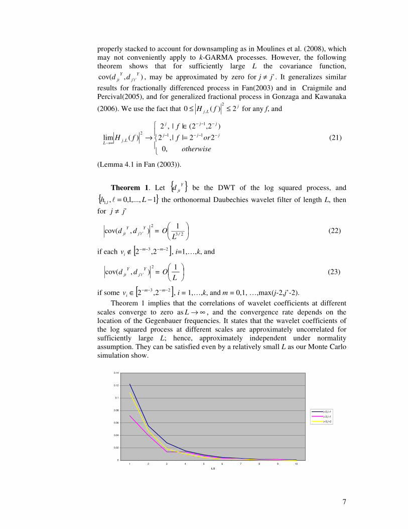
Theorem 1 implies that the correlations of wavelet coefficients at different scales converge to zero as ∞→L , and the convergence rate depends on the location of the Gegenbauer frequencies. It states that the wavelet coefficients of the log squared process at different scales are approximately uncorrelated for sufficiently large L; hence, approximately independent under normality assumption. They can be satisfied even by a relatively small L as our Monte Carlo simulation show.

0

0.02

0.04

0.06

0.08

0.1

0.12

0.14

1 2 3 4 5 6 7 8 9 10

L/2

j=2,j'=1

j=3,j'=1

j=3,j'=2

8

Figure 1. Absolute maximum values of between-scale correlations of a GARMA process

In Figure 1, we consider a GARMA process with d= 0.25 and v=0.35 using Daubechies wavelets D(L), L=2,4,…,10. Wavelet coefficients for scales 1≤ j’<j≤3 and max|Cov(djt,dj’t’)| for all possible values of t and t’ were obtained. In Figure 1, if j=2 and j’=1 the maximum correlation for the Haar wavelet is 0.1223, which decreases to 0.0006 when L=20. Faster decorrelation can be observed for larger |j-j’|. The approximation to zero of between-scale correlations is fairly accurate even for small values of L. For finite samples, this approximation does not depend on the length of the series, but the length of the wavelet filter which is under the control of the researcher. We proceed as if the wavelet coefficients at different scales are independent series when estimating the parameters of the GLMSV model.

For this purpose, we use the following result to approximate the spectral density of Y

jtd for sufficiently large L.

Theorem 2. Let { }Yjtd be the DWT coefficients of the log squared process,

and { }1,...,1,0,,1 −= Llh l the orthonormal Daubechies wavelet filter of length L,

then for 'jj = ,

),cov(lim)( )(2 Y

stjY

jtLj dds +∞→=σ = ( )dffSe j

fsi π22/1

2/1�

−

(24)

where where ( ) [ ]( ) [ ] [ ]( ) [ ] )(12)(12: 00 fIfSfIfSfS fj

Yfj

Yj ≥−

<− −++= and has a

period of 1.

( )fS j is positive and symmetric around zero, and contains the information of

the passband ( ]jj −−− 2,2 1 of the spectral density ( )fSY . We use ( )fS j as a convenient approximation to the spectral density of the within-scale wavelet coefficients { }Y

jtd for sufficiently large L, the corresponding variance is given by

).0(: 22jj σσ = The theorem also implies that within-scale correlations of wavelet

coefficients of the GLMSV model do not converge to zero as ∞→L . Unlike a fractionally integrated process, which is almost flat on the passband ( ]jj −−− 2,2 1 , the SDF )( fSX of a k-factor GARMA process may vary considerably depending

on the location of the Gegenbauer frequency. Hence ),cov( )(Y

stjY

jt dd + may be

relatively large when the Gegenbauer frequency is in ( ]jj −−− 2,2 1 or in an appropriate passband for other wavelet transforms. Thus, wavelet-based methods for FI processes need not extend directly to GARMA processes.

For the proposed estimation procedure, we consider the following conditions: A1: The spectral density of { }Y

jtd is reasonably approximated by ( )fS j .

A2: The polynomials )(zΘ and )(zΦ have no common zeros, their zeros lie ouside the unit circle, and they satisfy the normalization condition

( ) 10)0( =Φ=Θ . A3: The long-memory parameters satisfy (2). A4: The GLMSV model is identifiable, that is, 2

ησ is known or { }tX is not white

9

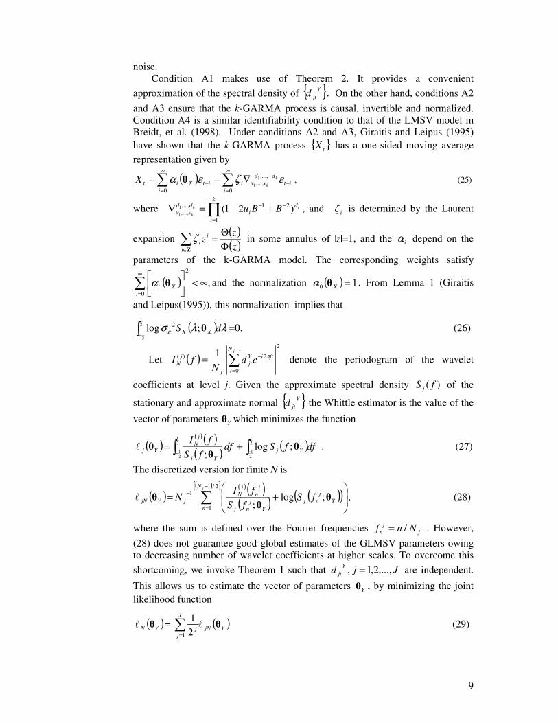
noise.

Condition A1 makes use of Theorem 2. It provides a convenient approximation of the spectral density of { }Y

jtd . On the other hand, conditions A2 and A3 ensure that the k-GARMA process is causal, invertible and normalized. Condition A4 is a similar identifiability condition to that of the LMSV model in Breidt, et al. (1998). Under conditions A2 and A3, Giraitis and Leipus (1995) have shown that the k-GARMA process { }tX has a one-sided moving average representation given by

( ) ��∞

=−

−−∞

=− ∇==

0

,...,,...,

0

1

1i

itdd

vvii

itXitk

kX εζεα � , (25)

where ∏=

−− +−=∇k

i

di

ddvv

ik

kBBu

1

21,...,,..., )21(1

1, and iζ is determined by the Laurent

expansion ( )( )zz

zi

ii Φ

Θ=�∈Z

ζ in some annulus of |z|=1, and the iα depend on the

parameters of the k-GARMA model. The corresponding weights satisfy

( ) ,0

2

∞<��

���

��

∞

=iXi �α and the normalization ( ) 10 =X�α . From Lemma 1 (Giraitis

and Leipus(1995)), this normalization implies that

( ) λλσ ε dS XX�−−2

1

21

;log 2� =0. (26)

Let ( )21

0

2)( 1�

−

=

−=jN

t

ftiYjt

j

jN ed

NfI π denote the periodogram of the wavelet

coefficients at level j. Given the approximate spectral density )( fS j of the

stationary and approximate normal { }Yjtd the Whittle estimator is the value of the

vector of parameters Y� which minimizes the function

( )Yj �� =( )( )( ) ( )dffSdffS

fIYj

Yj

jN� �− −

+21

21

21

21

;log;

��

. (27)

The discretized version for finite N is

( )YjN �� =( )( )( ) ( )( )

( )[ ]�

−

=

−

�

��

�+

2/1

1

1 ;log;

jN

nY

jnj

Yj

nj

jn

jN

j fSfS

fIN �

�, (28)

where the sum is defined over the Fourier frequencies jj

n Nnf /= . However, (28) does not guarantee good global estimates of the GLMSV parameters owing to decreasing number of wavelet coefficients at higher scales. To overcome this shortcoming, we invoke Theorem 1 such that Jjd Y

jt ,...,2,1, = are independent.

This allows us to estimate the vector of parameters Y� , by minimizing the joint likelihood function

( )YN �� = ( )YjN

J

jj ���

=1 21

(29)

10

where NJ 2log≤ . The weight N

N jj =

21 is proportional to the length of the

passband ( ]jj −−− 2,2 1 and the number of wavelet coefficients at level j, Nj.

We apply the normalization ( ) ( )YjjYj fSfS �� ;; 2* −= σ such that

( ) 0;log21

21

* =�− dffS Yj � . The likelihood functions in (27) and (28) reduce to

( )Yj �*� =

( )( )( )�−

21

21 ;* df

fSfI

Yj

jN

� (30)

and

( )YjN �*� =

( )( )( )

[ ]�

−

=

−

�

��

�2/)1(

1*

1

;

jN

n Yj

nj

jn

jN

j fSfI

N�

, (31)

respectively, with ( )YjNNY

j�� �

Θ= minargˆ . Thus, the likelihood function

corresponding to (29) is given by

( )YN �*� = ( ),

21 *

1YjN

J

jj ���

=

(32)

where NJ 2log≤ . The estimator is denoted by ( )YNNY ��

*minargˆ �Θ

= .

In the following theorem we show that the wavelet-based Whittle estimator defined by (32) is consistent. The proof is a modification of the proof of Theorem 1 of Breidt, et al. (1998).

Theorem 3. Let assumptions A1- A3 be satisfied, and let the parameter vectors 1

Y� and 2Y� be elements of the compact parameter space YΘ such that for

one j ( )1* ; Yj fS � = ( )2* ; Yj fS � implies that 21YY �� = . Then 0ˆ

YpNY �� → almost

surely as ∞→N , where 0Y� denotes the vector of true parameters.

The wavelet Whittle estimator in (32) is also consistent for each scale j. This provides an alternative local Whittle estimator of the GLMSV parameters by properly selecting the scales j corresponding to the frequencies in the neighborhood of the pole. This is only possible when the poles are known, in which case localization is done by selecting appropriate scales depending on the location of Gegenbauer frequencies and using the asymptotic property of the squared gain function in (21). However, this suffers from decreasing number of wavelet coefficients at higher scales, and it is not within the purview of this research.

In the absence of the additive noise { }tη , (9) is just the spectral density of a k-

GARMA process. Only in the case 02 =ησ we can write

( )��=

−−

J

jXjX dffS

1

221

21

;log �σ = ( )��=

−−

−−

J

jXXX dffS

j

j

1

2

2

21

;log2 �σ

( )dffS XXX�−≈ 2

1

0

2 ;log2 �σ = 0, (33)

when J is sufficiently large. The reduced wavelet Whittle likelihood function is

11

( )( )( )( )

[ ],

';1

'1

2/)1(

1

2 � �=

−

=

�

��

�=

J

j

N

n Xj

nj

jn

jN

X

j

fSfI

N ��εσ (34)

where ( ).,...,,,...,,,...,,,...,' 1111 pqkkX ddvv φφθθ=� are the parameters of a k-GARMA process. A similar formulation holds for the standard Whittle likelihood in (10).

5. Simulations and Application

Table 1. Monte Carlo simulations for GARMA models

Model

(v,d)

n

Method and

Wavelet v̂ d̂

Mean Bias rmse mean bias rmse

(0.05,0.3) 128

W-DWPT 0.0533 0.0033 0.0387 0.2815 -0.0185 0.0510

WE 0.0524 0.0024 0.0180 0.2930 -0.0070 0.0478

WWE 0.0527 0.0027 0.0119 0.2802 -0.0197 0.0544

512 W-DWPT 0.0483 -0.0017 0.0089 0.2848 -0.0152 0.0400

WE 0.0501 0.0001 0.0025 0.2941 -0.0005 0.0245

WWE 0.0501 0.0001 0.0025 0.2911 -0.0089 0.0219

1024 W-DWPT 0.0526 0.0026 0.0030 0.2901 -0.0100 0.0296

WE 0.0501 0.0001 0.0017 0.2910 -0.0090 0.0188

WWE 0.0499 -0.0001 0.0013 0.2919 -0.0081 0.0168

(0.3, 0.2) 128 W-DWPT 0.3084 0.0084 0.0927 0.1817 -0.0183 0.0843

WE 0.3115 0.0115 0.0557 0.1962 -0.0038 0.0727

WWE 0.3049 0.0049 0.0226 0.2025 0.0025 0.0653

512 W-DWPT 0.3020 0.0020 0.0490 0.1916 -0.0084 0.0469

WE 0.3019 0.0019 0.0170 0.1987 -0.0013 0.0300

WWE 0.2999 0.0001 0.0060 0.1932 -0.0068 0.0294

1024 W-DWPT 0.2971 -0.0029 0.0320 0.1904 -0.0096 0.0326

WE 0.3001 0.0001 0.0033 0.1917 0.0083 0.0218

WWE 0.3001 0.0001 0.0030 0.1971 -0.0029 0.0193

(0.45,0.3) 128 W-DWPT 0.4450 -0.0050 0.0387 0.2842 -0.0158 0.0529

WE 0.4486 -0.0014 0.0095 0.2886 -0.0114 0.0447

WWE 0.4478 -0.0022 0.0090 0.2959 -0.0041 0.0478

512 W-DWPT 0.4505 0.0005 0.0200 0.2878 -0.0122 0.0361

WE 0.4502 0.0002 0.0027 0.2934 -0.0066 0.0200

WWE 0.4502 0.0002 0.0025 0.2919 -0.0081 0.0227

1024 W-DWPT 0.4492 -0.0008 0.0108 0.2904 -0.0096 0.0241

WE 0.4501 0.0001 0.0014 0.2918 -0.0082 0.0166

WWE 0.4501 0.0001 0.0012 0.2924 -0.0076 0.0162

12

In this section, we assess the performance of the proposed methods by Monte Carlo simulation and application. We compare the performance of the wavelet Whittle estimator (WWE) in (29) with the standard Whittle estimator (WE) in (10), and the DWPT approximate MLE (W-DWPT) of Whitcher(2004) in estimating a pure k-GARMA process with Gaussian innovations. In the presence of the additive noise { }tη , we compare the wavelet Whittle estimator (G-WWE) in (29) with the Whittle estimator (G-WE) in (10), and we distinguish between Gaussian and standardized t-distributed te . Finally, we apply G-WWE in modeling the intraday seasonal patterns of Microsoft Stock realized volatility.

Table 2. Monte Carlo simulations for GARMA models

Model

(v,d)

n Method and

Wavelet v̂ d̂

Mean Bias rmse mean bias rmse

(0.2,0.1) 128

W-DWPT 0.2347 0.0347 0.1515 0.0900 -0.0100 0.0625

WE 0.2111 0.0111 0.0962 0.1041 0.0041 0.0557

WWE 0.2033 0.0033 0.0403 0.1108 0.0108 0.0545

512 W-DWPT 0.1883 -0.0117 0.0960 0.0889 -0.0111 0.0462

WE 0.2091 0.0091 0.0703 0.1024 0.0024 0.0429

WWE 0.2001 0.0001 0.0235 0.0992 -0.0008 0.0339

1024 W-DWPT 0.1863 -0.0137 0.0674 0.0928 -0.0072 0.0333

WE 0.2010 0.0010 0.0232 0.0980 -0.0020 0.0240

WWE 0.2003 0.0003 0.0134 0.0982 -0.0018 0.0200

(0.3,0.4) 128 W-DWPT 0.3023 0.0023 0.0511 0.3623 -0.0377 0.0845

WE 0.3004 0.0004 0.0086 0.3873 -0.0127 0.0604

WWE 0.3002 0.0002 0.0050 0.3921 -0.0079 0.0525

512 W-DWPT 0.3008 0.0008 0.0088 0.3708 -0.0292 0.0514

WE 0.2998 -0.0002 0.0016 0.4031 0.0031 0.0259

WWE 0.2999 0.0001 0.0013 0.3999 -0.0001 0.0279

1024 W-DWPT 0.3005 0.0005 0.0035 0.3789 -0.0211 0.0403

WE 0.2999 -0.0001 0.0007 0.3978 -0.0022 0.0159

WWE 0.2999 -0.0001 0.0006 0.3968 -0.0032 0.0189

(0.1,0.45) 128 W-DWPT 0.1121 0.0121 0.0405 0.4230 -0.0270 0.0537

WE 0.1001 0.0001 0.0049 0.4351 -0.0149 0.0425

WWE 0.0996 -0.0004 0.0036 0.4348 -0.0152 0.0468

512 W-DWPT 0.1045 0.0045 0.0348 0.4270 -0.0230 0.0508

WE 0.0999 -0.0001 0.0010 0.4476 -0.0023 0.0187

WWE 0.0999 -0.0001 0.0009 0.4449 -0.0051 0.0314

1024 W-DWPT 0.1023 0.0023 0.0311 0.4319 -0.0181 0.0408

WE 0.1001 0.0001 0.0006 0.4494 -0.0006 0.0168

WWE 0.1001 -0.0001 0.0005 0.4495 -0.0005 0.0155

13

Table 1 shows the Monte Carlo simulation results of GARMA models for 500 iterations, with poles at different frequencies in the absence of the additive noise { }tη . One pole is close to frequency 0, one close to 0.25 and one close to 0.5. The d-values are 0.2 and 0.3 respectively. In Table 2, we further consider GARMA models with parameters (v,d) = (0.2,0.1),(0.3,0.4), and (0.1,0.45). Actually we implemented different versions of wavelet filters, the extremal phase (D(L)), the least asymmetric (LA(L)), and minimum bandwidth (MB(L)) wavelet filters. We only present the results using the MB(16) wavelet filters, which provide more efficient estimates with respect to the filter length. Parallel results using MB(4) are omitted for brevity.

Results in Table 1 and Table 2 show that the WWE and WE estimates have smaller biases and root mean squared errors (RMSE) than W-DWPT for both the frequency v and the long-memory parameter d. Moreover, WWE generally performs better than WE in estimating the frequency v. This illustrates the advantage of wavelet method in locating discontinuities. In general, increase in sample size improves all estimates. On the other hand, increase in the length of the wavelet filter from 4 to 16 provides some improvement in the quality of the estimates of v and d.

14

Table 3 Confidence intervals corresponding to parameters (v,d) in Table 1 and Table 2

Table 3 shows 95% confidence intervals corresponding to the parameters d

and v in Table 1 and Table 2. The symbol * indicates that the confidence interval does not overlap with the corresponding interval for WWE, which implies that the corresponding estimates are significantly different. Most of these intervals correspond to W-DWPT estimates.

n

Method and

Wavelet

95% Confidence Interval for v

(Table 1)

95% Confidence Interval for d

(Table 1)

95% Confidence Interval for v

(Table 2)

95% Confidence Interval for d

(Table 2)

128

W-DWPT (0.0499,0.0567) (0.2773, 0.2857) (0.2218,0.2476)* (0.0846,0.0954)*

WE (0.0508,0.0540) (0.2889,0.2971)* (0.2027,0.2195) (0.0992,0.1090)

WWE (0.0517,0.0537) (0.2758, 0.2846) (0.1998,0.2068) (0.1061,0.1155)

512 W-DWPT (0.0475,0.0491)* (0.2816,0.2880)* (0.1799,0.1967)* (0.0850,0.0928)*

WE (0.0499,0.0503) (0.2920,0.2962) (0.2030,0.2152)* (0.0986,0.1062)

WWE (0.0499,0.0503) (0.2893,0.2929) (0.1980,0.2022) (0.0962,0.1022)

1024 W-DWPT (0.0525,0.0527) (0.2877,0.2925) (0.1805,0.1921)* (0.0900,0.0956)*

WE (0.0500,0.0502) (0.2896,0.2924) (0.1990,0.2030) (0.0959,0.1001)

WWE (0.0498,0.0500) (0.2906,0.2932) (0.1991,0.2015) (0.0965,0.0999)

128 W-DWPT (0.3003,0.3165) (0.1745,0.1889)* (0.2978,0.3068) (0.3557,0.3689)*

WE (0.3067,0.3163) (0.1898,0.2026) (0.2996,0.3012) (0.3821,0.3925)

WWE (0.3030,0.3068) (0.1968,0.2082) (0.2998,0.3006) (0.3876,0.3966)

512 W-DWPT (0.2977,0.3063) (0.1876,0.1956) (0.3000,0.3016) (0.3671,0.3745)*

WE (0.3004,0.3034) (0.1961,0.2013)* (0.2997,0.2999) (0.4008,0.4054)

WWE (0.2994,0.3004) (0.1907,0.1957) (0.2998,0.3000) (0.3975, 0.4023)

1024 W-DWPT (0.2943,0.2999) (0.1877,0.1931)* (0.3002,0.3008)* (0.3759,0.3819)*

WE (0.2998,0.3004) (0.1899,0.1935)* (0.2998,0.3000) (0.3964,0.3992)

WWE (0.2998,0.3004) (0.1954,0.1988) (0.2998,0.3000) (0.3952,0.3984)

128 W-DWPT (0.4416,0.4484) (0.2798,0.2886)* (0.1087,0.1155)* (0.4189,0.4271)*

WE (0.4478,0.4494) (0.2848,0.2924) (0.0997,0.1005) (0.4316,0.4386)

WWE (0.4470,0.4486) (0.2917,0.3001) (0.0993,0.0999) (0.4309,0.4387)

512 W-DWPT (0.4487,0.4523) (0.2848,0.2908) (0.1015,0.1075)* (0.4230,0.4310)*

WE (0.4500,0.4504) (0.2917,0.2951) (0.0998,0.1000) (0.4460,0.4492)

WWE (0.4500,0.4504) (0.2900,0.2938) (0.0998,0.1000) (0.4422,0.4476)

1024 W-DWPT (0.4483,0.4501) (0.2885,0.2923) (0.0996,0.1050) (0.4287,0.4351)*

WE (0.4500,0.4502) (0.2905,0.2931) (0.1000,0.1002) (0.4479,0.4509)

WWE (0.4500,0.4502) (0.2911,0.2937) (0.1001,0.1001) (0.4481,0.4509)

15

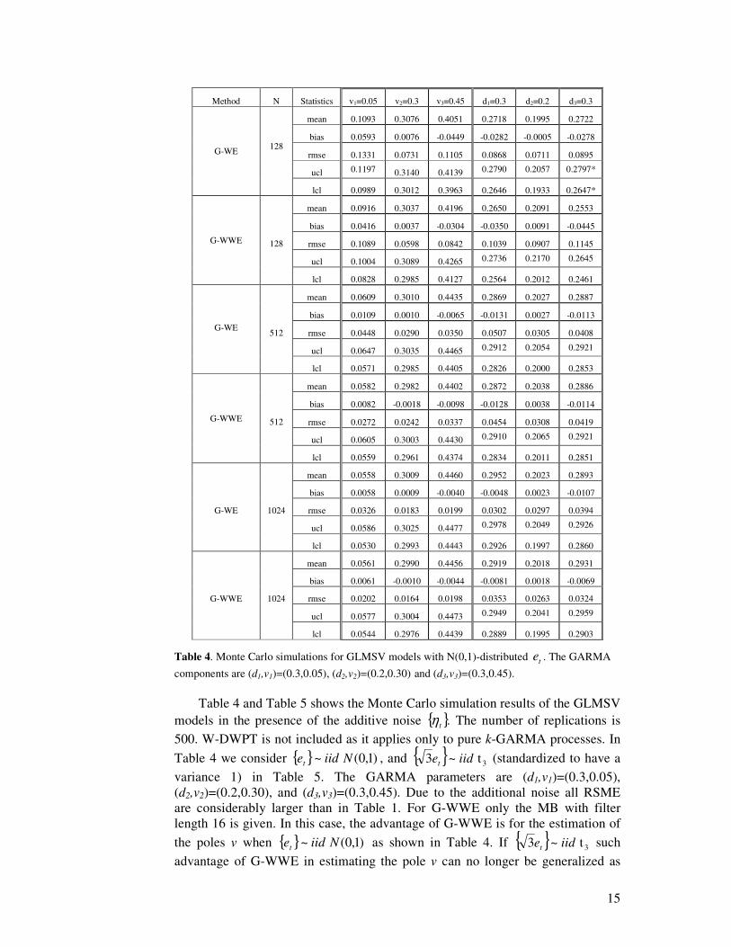
Table 4. Monte Carlo simulations for GLMSV models with N(0,1)-distributed te . The GARMA components are (d1,v1)=(0.3,0.05), (d2,v2)=(0.2,0.30) and (d3,v3)=(0.3,0.45).

Table 4 and Table 5 shows the Monte Carlo simulation results of the GLMSV

models in the presence of the additive noise { }.tη The number of replications is

500. W-DWPT is not included as it applies only to pure k-GARMA processes. In Table 4 we consider { } )1,0( ~ Niidet , and { } 3 t~3 iidet (standardized to have a variance 1) in Table 5. The GARMA parameters are (d1,v1)=(0.3,0.05), (d2,v2)=(0.2,0.30), and (d3,v3)=(0.3,0.45). Due to the additional noise all RSME are considerably larger than in Table 1. For G-WWE only the MB with filter length 16 is given. In this case, the advantage of G-WWE is for the estimation of the poles v when { } )1,0( ~ Niidet as shown in Table 4. If { } 3 t~3 iidet such advantage of G-WWE in estimating the pole v can no longer be generalized as

Method N Statistics v1=0.05 v2=0.3 v3=0.45 d1=0.3 d2=0.2 d3=0.3

G-WE 128

mean 0.1093 0.3076 0.4051 0.2718 0.1995 0.2722

bias 0.0593 0.0076 -0.0449 -0.0282 -0.0005 -0.0278

rmse 0.1331 0.0731 0.1105 0.0868 0.0711 0.0895

ucl 0.1197 0.3140 0.4139 0.2790 0.2057 0.2797*

lcl 0.0989 0.3012 0.3963 0.2646 0.1933 0.2647*

G-WWE 128

mean 0.0916 0.3037 0.4196 0.2650 0.2091 0.2553

bias 0.0416 0.0037 -0.0304 -0.0350 0.0091 -0.0445

rmse 0.1089 0.0598 0.0842 0.1039 0.0907 0.1145

ucl 0.1004 0.3089 0.4265 0.2736 0.2170 0.2645

lcl 0.0828 0.2985 0.4127 0.2564 0.2012 0.2461

G-WE 512

mean 0.0609 0.3010 0.4435 0.2869 0.2027 0.2887

bias 0.0109 0.0010 -0.0065 -0.0131 0.0027 -0.0113

rmse 0.0448 0.0290 0.0350 0.0507 0.0305 0.0408

ucl 0.0647 0.3035 0.4465 0.2912 0.2054 0.2921

lcl 0.0571 0.2985 0.4405 0.2826 0.2000 0.2853

G-WWE 512

mean 0.0582 0.2982 0.4402 0.2872 0.2038 0.2886

bias 0.0082 -0.0018 -0.0098 -0.0128 0.0038 -0.0114

rmse 0.0272 0.0242 0.0337 0.0454 0.0308 0.0419

ucl 0.0605 0.3003 0.4430 0.2910 0.2065 0.2921

lcl 0.0559 0.2961 0.4374 0.2834 0.2011 0.2851

G-WE 1024

mean 0.0558 0.3009 0.4460 0.2952 0.2023 0.2893

bias 0.0058 0.0009 -0.0040 -0.0048 0.0023 -0.0107

rmse 0.0326 0.0183 0.0199 0.0302 0.0297 0.0394

ucl 0.0586 0.3025 0.4477 0.2978 0.2049 0.2926

lcl 0.0530 0.2993 0.4443 0.2926 0.1997 0.2860

G-WWE 1024

mean 0.0561 0.2990 0.4456 0.2919 0.2018 0.2931

bias 0.0061 -0.0010 -0.0044 -0.0081 0.0018 -0.0069

rmse 0.0202 0.0164 0.0198 0.0353 0.0263 0.0324

ucl 0.0577 0.3004 0.4473 0.2949 0.2041 0.2959

lcl 0.0544 0.2976 0.4439 0.2889 0.1995 0.2903

16

shown in Table 5. However, only one interval (indicated by *) does not overlap with the corresponding interval for G-WWE of the same parameter and sample size. This implies that most G-WWE and G-WE estimates are in Table 1 and Table 2 are not significantly different under normality assumption.

Table 5. Monte Carlo simulations for GLMSV models with t-distributed te . The GARMA components are (d1,v1)=(0.3,0.05), (d2,v2)=(0.2,0.30) and (d3,v3)=(0.3,0.45).

Performing this Monte Carlo study we observe that the estimates of the

GARMA parameters are significantly affected by the initial value of 2ησ , which is

usually unknown in practice, but can be estimated from the wavelet coefficients of

Method N Statistics v1=0.05 v2=0.3 v3=0.45 d1=0.3 d2=0.2 d3=0.3

G-WE 128

mean 0.1108 0.3060 0.4078 0.2652 0.2070 0.2640

bias 0.0608 0.0060 -0.0422 -0.0348 0.0070 -0.0360

rmse 0.1373 0.0685 0.1006 0.1041 0.0825 0.1006

ucl 0.1216 0.3120 0.4158* 0.2738 0.2142 0.2722

lcl 0.1000 0.3000 0.3998* 0.2566 0.1998 0.2558

G-WWE 128

mean 0.0971 0.3075 0.4270 0.2480 0.2003 0.2547

bias 0.0471 0.0075 -0.0230 -0.0520 0.0003 -0.0453

rmse 0.1194 0.0646 0.0636 0.1233 0.0924 0.1179

ucl 0.1067 0.3131 0.4322 0.2578 0.2084 0.2642

lcl 0.0875 0.3019 0.4218 0.2382 0.1922 0.2452

G-WE 512

mean 0.0638 0.2978 0.4405 0.2855 0.2041 0.2822

bias 0.0138 -0.0022 -0.0095 -0.0145 0.0041 -0.0178

rmse 0.0569 0.0301 0.0341 0.0553 0.0467 0.0582

ucl 0.0686 0.3004 0.4434 0.2902 0.2082 0.2871

lcl 0.0590 0.2952 0.4376 0.2808 0.2000 0.2773

G-WWE 512

mean 0.0614 0.2970 0.4419 0.2804 0.2055 0.2844

bias 0.0114 -0.0030 -0.0081 -0.0196 0.0055 0.0156

rmse 0.0411 0.0335 0.0299 0.0628 0.0404 0.0551

ucl 0.0649 0.2999 0.4444 0.2856 0.2090 0.2890

lcl 0.0579 0.2941 0.4394 0.2752 0.2020 0.2798

G-WE 1024

mean 0.0546 0.2998 0.4468 0.2920 0.2016 0.2898

bias 0.0046 -0.0002 -0.0032 -0.0080 0.0016 -0.0102

rmse 0.0240 0.0145 0.0138 0.0367 0.0213 0.0388

ucl 0.0567 0.3010 0.4480 0.2951 0.2035 0.2931

lcl 0.0525 0.2985 0.4456 0.2889 0.1997 0.2865

G-WWE 1024

mean 0.0568 0.2988 0.4465 0.2911 0.2015 0.2897

bias 0.0068 -0.0012 -0.0035 -0.0089 0.0015 -0.0103

rmse 0.0312 0.0200 0.0148 0.0315 0.0268 0.0348

ucl 0.0595 0.3005 0.4478 0.2937 0.2038 0.2926

lcl 0.0541 0.2971 0.4452 0.2885 0.1992 0.2868

17

the log-squared process. Conventional estimates include the sample standard deviation, LP norms, and the median absolute deviation (MAD) of the wavelet coefficients. The MAD is known to be a robust estimator of scale, which exists even for some distributions with nonexistent mean or variance. We found out that the use of the square of the MAD of the wavelet coefficients of the log-squared process at level 1 as the initial value of 2

ησ provides better estimates for the long-memory parameters than standard estimators. The heuristic argument for the choice of level 1 wavelet coefficients is that they are noise dominated. We use this initial value in the ensuing application.

Figure 2. Log-periodogram and estimated spectrum of tt rvY =

For illustrative purpose the proposed method is applied to modeling the

intraday seasonal patterns of Microsoft stock realized volatility, trv , using tick data sampled every minute. The data cover 140 trading days in the period August 5, 2008 to November 26, 2008 each 9:30 to 16:00, with 391 prices per day. Returns are defined as ( ) ( ) ( )( )δδδ 1−+−+=+ mtpmtpmtr , where ( )Pp log= , m=1,…,390, δ is 1/390, i.e. 1 minute, and t=1,…140. P denotes the prices of the share. We consider realized volatility at 30-minutes intervals

( ) ( )( )[ ]�=

+−+=30

1

2130,;m

mhtrhtrv δδ with h=1,…,13. (See Andersen et al.(2003))

For instance, ( )δ,3;2rv is the realized volatility of third half hour period of the second day. So a total of 13x140 observations are available, using the first

102=N . Overnight returns are ignored as we are interested primarily in the intraday seasonal pattern.

18

The log-periodogram of the Yt series in Figure 2 of the Microsoft stock intraday realized volatility seems to indicate 2 to 4 strong seasonal components with varying decay. Hence, an SV model based on the seasonal fractional process of the form tt

dS XB ε=− )1( may not be the appropriate model since it assumes exactly S=7 poles on [0, 0.5] with the same long-memory parameter d. Hence we use the GLMSV model to represent the Yt series.

We start estimating the stochastic volatility model with a one-factor GARMA component (one pole) for Xt. Then we successively add more seasonal components into the model. For this purpose, we use the Akaike Information Criterion (AIC) for model selection. The AIC is a penalized log-likelihood defined by ( ) plikelihood 2log2 +−− , where p is the number of parameters in the

model. The parameter estimates for the 1-GARMA are d̂ = 0.2364 and v̂ =0. The corresponding value of the AIC is -725.2532. We then estimate a two-factor GARMA model with AIC=-806.7974. The smaller AIC for this two-factor model indicates the need for inclusion of two more parameters in order to fit an additional singularity in the spectrum. Any further increase in the number of poles does not result in a decrease of the AIC. The inclusion of ARMA parameters does not decrease the AIC either. Therefore, the final model is a two-factor GARMA with long-memory parameters 0.1218 and 0.2256 at the poles 0, 0.0772, respectively. The model is given by

( ) ( )( ) ( ) tt YYBBBB επ =−+−+− 2256.021218.02 )0772.0(2cos2121 . (34)

The poles are 0.0772 and 0, each represents the kth intraday seasonal frequency (normalized), Nkfk /= , where N is the number of data points. Since k = 0.0772N � N /13, then the frequency fk = 0.0772 corresponds to the period of 13 half-hours or 7.5 hours. On the other hand, the frequency 0 corresponds to an infinite period representing the FI component. In Figure 1, these poles are the first two prominent peaks of the periodogram. Comparing periodogram and estimated spectrum the ignorance of other seasonal poles seems to be remarkable. Assuming that GLMSV is the true model this might indicate that larger sample sizes are required than for other models to extract the features of the series due to the additional error.

6. Concluding Remarks

In this paper, we proposed a generalization of the LMSV model, and a wavelet Whittle estimator of its parameters based on the properties of its wavelet coefficients that we derived. The approach takes advantage of the wavelet transform’s ability in detecting poles, separating noise from the process, and the asymptotic normality of the wavelet coefficients.

Simulation results have shown that in the absence of the additive noise, the proposed method (WWE) performs better than the approximate DWPT MLE (W-DWPT) and comparable to the standard Whittle estimator (WE). In the presence of the additive noise, the proposed method (G-WWE) performs generally better than the standard Whittle estimator (G-WE) in estimating the poles, except when the error term is not normally distributed. In estimating the long-memory parameters, G-WE is relatively comparable to G-WWE when L=16, and improves as the filter length L increases. In modeling the Microsoft stock intraday volatility we find a GLMSV with k=2.

19

We have also shown that the proposed estimator is consistent. Other properties of the estimators still need to be derived, particularly the limiting distributions which will provide tests of significance of estimated values. The theoretical properties of the Whittle estimators of k-GARMA are not yet completely known for k>1. If k=1, a relatively complete account of asymptotic properties is given in Giraitis, Hidalgo and Robinson (2001). The GLMSV model is even more general and complicated than a k-GARMA model. To our knowledge no proof for the GLM part has been published more recently. The argument of Deo(1995) for the stochastic volatility LM model rests on the previous proof for the asymptotic distribution of the LM part. The derivation of the asymptotic distribution of our proposed estimator would have to take into account the long-memory property, the k poles, and the within-scale correlations of the wavelet coefficients. We think this is worth being dealt with in a separate paper, which is currently under work. Forecast comparisons with other approaches such as the one proposed in Deo, Hurvich and Lu (2006) are desirable directions for future research.

Appendices A. Proof of Theorem 1

Let )( fSY be the SDF of the log squared process. Without loss of generality, assume that j>j’. From (20), we have

2

'' ),cov( Ytj

Yjt dd ≤

20

0,',0 )(|)(||)(|

���

�� dffSfHfHc YLjLj , (35)

for some constant c0 independent of L (ci, i=0,1,2,… will be used to denote a constant independent of L). By Cauchy-Schwarz inequality, we have

2

'' ),cov( Ytj

Yjt dd ≤

���

�� ∏

−

=

− dffSfGfc Y

j

m

mL

j )()2(|)2(H|5.0

0

2

0

2

,121'

L1,0

���

�� dffSfx Y )(|)(H|5.0

0

2*Lj,

, (36)

where ∏−

=

−=2'

0

2

,1

21,1

2*, )2()2(|)(|

j

m

mL

jLLj fGfHfH . Since j

Lj fH 2)(02

, ≤≤ , the

second factor in (36) is finite, that is

dffSf Y )(|)(H|5.0

0

2*Lj,� ( )( ) ∞<+=≤ 22)(2 ησt

jt

j XVarYVar . (37)

We now show that the first factor in (36) converges to 0 as ∞→L , and obtain its order of convergence. By partitioning the interval of integration, we get

dffSfGf Y

j

m

mL

j )()2(|)2(H|5.0

0

2

0

2

,121'

L1,� ∏−

=

− ≤ c1 A1 + c2 A2, (38)

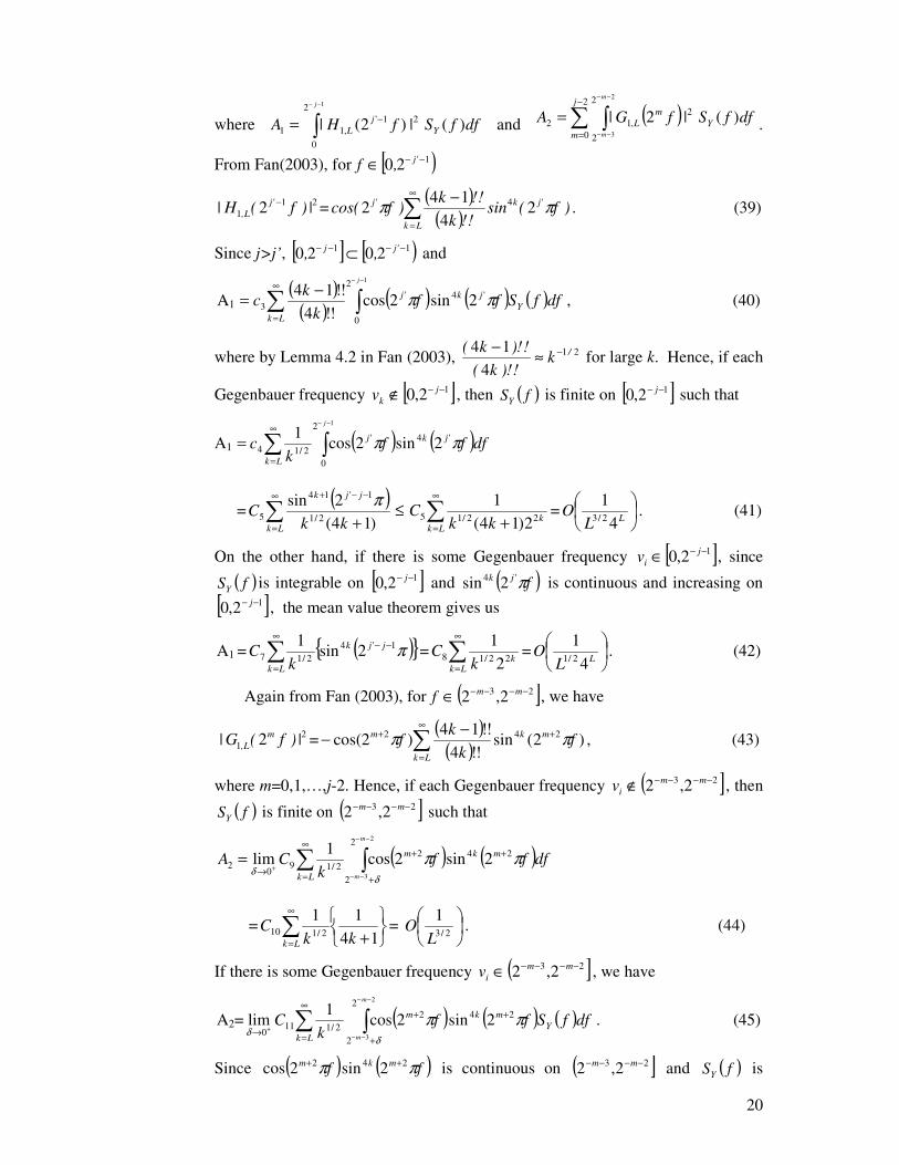
20

where �−−

−=12

0

21',11 )(|)2(|

j

dffSfHA Yj

L and ( )� �−

=

−−

−−

=2

0

2

2

2,12

2

3

)(|2|j

mY

mL

m

m

dffSfGA .

From Fan(2003), for [ )120 −−∈ 'j,f

211 2 |)f(H| 'j

L,− =

( )( ) )f(sin

!!k!!k

)fcos( 'jk

Lk

'j ππ 24

142 4�

∞

=

−. (39)

Since j>j’, [ ] [ )11 2020 −−−− ⊂ 'jj ,, and

A1 ( )

( ) ( ) ( ) ( )��−−

∞

=

−=12

0

'4'3 2sin2cos

!!4!!14

j

dffSffk

kc Y

jkj

Lk

ππ , (40)

where by Lemma 4.2 in Fan (2003), 21

414 /k

!)!k(!)!k( −≈−

for large k. Hence, if each

Gegenbauer frequency [ ]12,0 −−∉ jkv , then ( )fSY is finite on [ ]12,0 −− j such that

A1 ( ) ( )��−−

∞

=

=12

0

'4'2/14 2sin2cos

1j

dfffk

c jkj

Lk

ππ

=( )

�∞

=

−−+

+Lk

jjk

kkC

)14(2sin

2/1

1'14

5π ≤ �

∞

= +Lkkkk

C 22/15 2)14(1

=

��

�LL

O4

12/3 . (41)

On the other hand, if there is some Gegenbauer frequency [ ]12,0 −−∈ jiv , since

( )fSY is integrable on [ ]12,0 −− j and ( )fjk π'4 2sin is continuous and increasing on [ ]12,0 −− j , the mean value theorem gives us

A1 = ( ){ }π1'42/17 2sin

1 −−∞

=� jjk

Lk kC = �

∞

=Lkkk

C 22/18 21

=

��

�LL

O4

12/1 . (42)

Again from Fan (2003), for ( ]23 2,2 −−−−∈ mmf , we have

21 2 |)f(G| m

L, =( )

( ) )2(sin!!4

!!14)2cos( 242 f

kk

f mk

Lk

m ππ +∞

=

+ �−− , (43)

where m=0,1,…,j-2. Hence, if each Gegenbauer frequency ( ]23 2,2 −−−−∉ mmiv , then

( )fSY is finite on ( ]23 2,2 −−−− mm such that

( ) ( )��−−

−−+

+

++∞

=→=

2

3

2

2

2422/19

02 2sin2cos

1lim

m

m

dfffk

CA mkm

Lk δδ

ππ

=���

���

+�∞

= 1411

2/110 kkC

Lk

=

��

�2/3

1L

O . (44)

If there is some Gegenbauer frequency ( ]23 2,2 −−−−∈ mmiv , we have

A2= ( ) ( ) ( )� �∞

= +

++

→

−−

−−+

LkY

mkm

m

m

dffSffk

C2

3

2

2

2422/111

02sin2cos

1lim

δδ

ππ . (45)

Since ( ) ( )ff mkm ππ 242 2sin2cos ++ is continuous on ( ]23 2,2 −−−− mm and ( )fSY is

21

integrable on ( ]23 2,2 −−−− mm , the mean value theorem gives us

A2 [ ] ( ) ( ) ( )� �∞

= +

++

∈→

−−

−−−−−−+ ��

����≤

LkY

mkm

f

m

mmm

dffSffk

C2

323

2

2

242

2,22/1110

2sin2cosmax1

limδ

δππ , (46)

where [ ]

( ) ( )[ ] ( )π

ππ 2

1242

2,2 22tan

2sin2cosmaxarg23

+

−++

∈=

−−−− mmkm

f

kff

mm. Moreover,

A2 ( )( ) ( )( )[ ]�∞

=

−−=Lk

k kkk

C 2tansin2tancos1 141

2/112

�∞

=��

���

�

+=

Lk kkC

1411

2/113 =

��

�

LO

1, (47)

where (47) is obtained using the identities

���

�

+= −−

1

1costan

2

11

xx for x>0, and

���

�

+= −−

1sintan

2

11

x

xx for all x (see e.g. Gradshteyn and Ryzhik (2007) p. 57).

The result follows from (41), (42), (44) and (47). QED.

B. Proof of Theorem 2

Setting j=j’ and t’=t+s in (20) the within-scale covariance of { }Y

jtd is given by

),cov( )(Y

stjY

jt dd + = �−

2/1

2/1

222, )(|)(| dffSefH Y

sfiLj

jπ . (48)

Partitioning the interval of integration, we get

),cov( )(Y

stjY

jt dd + = dffSefH Ysfi

SLj

j

)(|)(| 222,

π� +

dffSefH Y

S

sfiLj

j

)(|)(|*

222,�+ π (49)

Where ]2,2[]2,2[ 11 jjjjS −−−−−− ∪−−= and [ ] SS −−= 5.0,5.0* . Since j

Lj fH 2)(02

, ≤≤ for any f,

dffSefH Ysfi

Lj

j

�− ]5.0,5.0[

222, )(|)(| π

dffSYj )(2]5.0,5.0[

�−

≤ = ( )( ) ∞<+= 22)(2 ησtj

tj XVarYVar . (50)

Hence, )(|)(|)( 222, fSefHLg Y

sfiLj

jπ= is integrable on *SS ∪ . Moreover,

22

( ) )(2lim 22 fSeLg Ysfij

L

jπ=∞→

a.e. on S, ( ) 0lim =∞→

LgL

a.e. on S*, and

)(2 22 fSe Ysfij jπ is integrable on S by a similar argument to (50). Thus, by the

Lebesgue’s Dominated Convergence Theorem, we have

),cov(lim )(Y

stjY

jtLdd +∞→

= dffSeS

Ysfij j

� )(2 22π (51)

Now, using the transformation 12' −= ff j , we have

dffSeS

Ysfij j

� )(2 22π = [ ]( ) '1'2'2

'

dffSe jY

sfi

S

+−�

π , (52)

where ]0,[],2[' 21

23 −− ∪−=S . Thus,

),cov(lim )(Y

stjY

jtLdd +∞→

= ( )dffSe jfsi π2

2/1

2/1�

−

, (53)

where ( ) [ ]( ) [ ] [ ]( ) [ ] )(12)(12: 00 fIfSfIfSfS fj

Yfj

Yj ≥−

<− −++= and has a period of

1. QED

C. Proof of Theorem 3

Let Y� be an element of the compact parameter space YΘ . We also define

( )Yoj �� =

( )( ) ,

;

;21

21 *

0*

dffS

fS

Yj

Yj�− ��

���

��

���

�

� and ( ) ( )�=

jY

ojY

o�� �� . (54)

We then have

( ) ( )YojYNj �� �� −*

( )( )( )

( )[ ] ( )( ) Nj

Yj

YjN

r Yj

jN

j MdffS

fS

fSfI

Nj

=−≤ �� −

−

=

− 21

21 ;

;

; *

0*2/1

1*

1

�

�

� (55)

Now, NjM can be shown to converge to zero almost surely by modifying the proof of Lemma 1 of Hannan(1973) (see also proof of Theorem 1 in Breidt, et al.

(1998)). First, since ( )[ ] 1* ;−

Yj fS � is continuous in ( )Yf �, , the Cesaro sum of its

Fourier series converges uniformly in ( )Yf �, . Second, we show that the process

{ }t

Yjtd is ergodic. Using conditions A2 and A3, for each j =1,…,J we can write

the nonboundary wavelet coefficients of the log-squared process as

� −−+=

lltlj

Yjt jYhd

1)1(2, ( ) ,,0

ijt

ijt i ξαγ η �

∞

=Λ+= (56)

where � −−+=

lltljjt jh

1)1(2, ηγ η and ,1)1(2,� −−−+

=l

iltljijt jh εξ ,+∈ Zi are the new

innovations such that ( )[ ]�∞

=∞<

0

2,i

Xi �α . For ,+∈ Zi ijtξ are independent since tε

are independent, normally distributed, and DWT is an orthonormal transform.

23

Since tε are independent and

,12, =�

lljh then

( ) ( ) .varvar 21)1(2

2, εσεξ ==

−−−+� pltl

ljpjt jh

Similarly, ( ) .var 2

ηη σγ =jt Moreover, for

each ,+∈ Zi ijtξ and ηγ jt are independent since tη and tε are independent. Thus,

{ }yjtd is ergodic since ( )

���

����

∞

=

ijt

iXi ξα

0

,� and { }ηγ jt are independent linear processes

with iid innovations and square summable coefficients (see Hannan(1970) p. 204). Thus, by Lemma 1 of Hannan(1973), NjM converges to zero almost surely such that

( ) a.s. 0)(sup * →−Θ

YojYNj �� �� (57)

Since ( ) 0;log21

21

* =�− dffS Yj � and xx −≥− 1log , then

( )Yoj ��

( )( )

( )( ) ,

;

;

;

;log2

1

21 *

0*

*

0*

dffS

fS

fS

fS

Yj

Yj

Yj

Yj�− ��

���

��

���

+���

�

���

�−=

�

�

�

� (58)

( )( )

( )( ) ,

;

;

;

;12

1

21 *

0*

*

0*

dffS

fS

fS

fS

Yj

Yj

Yj

Yj�− ��

���

��

���

+−≥�

�

�

� (59)

( )( ) ).(

;

; 00*

0*21

21 Y

oj

Yj

Yj dffS

fS�

�

��=

��

���

��

���

= �− (60)

And using the identifiability condition, 0Y� uniquely minimizes )( Y

oj �� . This

implies that ( ) ( )nYojY

oj �� ˆ0

�� ≤ . Moreover, ( ) ( ) ( )0*** infˆYnjnYnjnYnj

Y

��� ��� ≤=Θ

. These

and (57) imply that ( )0)ˆ( YojnY

oj �� �� → a.s. for each j. Moreover, since

( )0)ˆ( Yo

NYo

�� �� − ( )�=

−≤J

jY

ojNY

ojj j

1

0)ˆ(21

�� �� a.s.,

( )�=

−≤J

jY

ojNY

oj j

1

0)ˆ(21

�� �� a.s. (61)

then ( )0)ˆ( Y

oNY

o�� �� → a.s. (62)

Therefore 0ˆYnY �� →

a.s. by compactness of YΘ .

References Andersen T, Bollerslev T (1997) Intraday periodicity and volatility persistence in financial markets. Journal of Empirical Finance 4: 115-158.

24

Andersen T, Bollerslev T, Diebold FX, Labys P (2003) Modeling and Forecasting Realized Volatility, Econometrica 71: 529-626. Arteche J (2004) Gaussian semiparametric estimation in long memory in stochastic volatility and signal plus noise models. Journal of Econometrics 119: 131-154. Arteche J, Robinson P (2000) Semiparametric Inference in Seasonal and cyclical long memory processes. Journal of Time Series Analysis 21(1):1-25. Bisaglia L, Bordignon S, Lisi F (2003) k-factor garma models for intraday volatility forecasting. Applied Economics Letters 10: 251-254. Breidt FJ, Crato N, de Lima P (1998) On the detection and estimation of long memory in stochastic volatility. Journal of Econometrics 83: 325-348. Bollerslev T, Mikkelsen HO (1996) Modeling and pricing long memory in stock market volatility. Journal of Econometrics 73:151-184. Bockina NA(2007) Wavelet goodness-of-fit test for dependent data. Journal of Statistical Planning and Inference 137: 2593-2612. Chung C (1996) Estimating a generalized long-memory process. Journal of Econometrics 73: 237-259. Craigmile PF, Percival DB (2005) Asymptotic decorrelation of between-scale wavelet coefficients. IEEE Trans. Info. Theory 51: 1039-1048 Daubechies I (1992) Ten Lectures on Wavelets. SIAM, Philadelphia Deo R, Hurvich C (2001) On the log periodogram regression estimator of the memory parameter in long memory stochastic volatility models. Econometric Theory 17:686-710 Deo R, Hurvich C, Lu Y (2006) Forecasting realized volatility using a long-memory stochastic volatility model: estimation, prediction and seasonal adjustment. Journal of Econometrics 131: 29-58 Fan Y (2003) On the Approximate Decorrelation Property of Discrete Wavelet Transform for Fractionally Differenced Process. IEEE Transactions on Information Theory 49:516-521. Giraitis L, Leipus R (1995) A generalized fractionally differencing approach in long-memory modeling. Lithuanian Mathematical Journal 35(1):53-65. Gonzaga A, Kawanaka A (2006) Asymptotic Decorrelation of Between-Scale Wavelet Coefficients of Generalized Fractional Process. Digital Signal Processing 16: 320-329. Gray H, Zhang N, Woodward W (1989) On Generalized Fractional Processes. Journal of Time Series Analysis 10(3):233-257.

25

Grandshteyn IS, Ryshik IM (1980) Table of Integrals, series, and products. Academic Press, Orlando, FL. Harvey A (1998) Long memory in stochastic volatility. In: Knight J, Satchell S (Eds.) Forecasting Volatility in Financial Markets. Butterworth-Heineman, Oxford, pp. 307-320. Hannan EJ (1970) Multiple Time Series. John Wiley and Sons, Inc., New York Hannan EJ (1973) The asymptotic theory of linear time-series models. Journal of Applied Probability 10(1):130-145. Hurvich C, Ray B (2003) The Local Whittle estimator of long-memory stochastic volatility. Journal of Financial Econometrics 1(3):445-470. Jensen M (2004) Semiparametric Bayesian Inference of Long-memory stochastic volatility models. Journal of Time Series Analysis 25(6): 895-122. Moulines E, Roueff F, Taqqu MS (2008) A wavelet whittle estimator of the memory parameter of a nonstationary Gaussian time series. Annals of Statistics 36(4):1925-1956. Palma W, Chan NH (2005) Efficient estimations of seasonal long range dependent processes. Journal of Time Series Analysis 26: 863 - 892. Percival DB, Sardy S and Davison AC (2001) Wavestrapping Time Series: Adaptive Wavelet-Based Bootstrapping, in W. J. Fitzgerald, R. L. Smith, A. T. Walden and P. C. Young (Eds.), Nonlinear and Nonstationary Signal Processing, Cambridge, England: Cambridge University Press 442-470. Percival D, Walden A (2000) Wavelet Methods for Time Series Analysis. Cambridge University Press Porter-Hudak S (1990) An application of seasonal fractionally differenced model to the monetary aggregates. JASA 85: 338-344. Soares LJ, Souza LR (2006) Forecasting electricity demand using generalized long memory. International Journal of Forecasting 22: 17-28. Taqqu M, Teverovsky V (1997) Robustness of Whittle-type Estimators for Time Series with Long-Range Dependence. Stochastic Models 13: 723-757. Whitcher B (2004) Wavelet-based estimation for seasonal long-memory. Technometrics 46(2): 225-238. Woodward W, Cheng Q, Gray H (1998) A k-factor GARMA Long-memory model. Journal of Time Series Analysis 19(4): 485-504.