A THERMODYNAMICALLY CONSISTENT FRAMEWORK FOR …
31
Pergamon ht. J. Solid.s S~rucrures Vol. 31, No. 3. pp. 359-389, 1994 0 1994 Elsevier Science Ltd Printed in Great Britain. All rights reserved 002&7683/94 $6.00 + .I0 A THERMODYNAMICALLY CONSISTENT FRAMEWORK FOR THEORIES OF ELASTOPLASTICITY COUPLED WITH DAMAGE N. R. HANSEN Sandia National Laboratories, Albuquerque, NM 87115, U.S.A. and H. L. SCHREYER Department of Mechanical Engineering, University of New Mexico, Albuquerque, NM 87131. U.S.A. (Recrived 7 December 1992 ; in revised,form 28 July 1993) Abstract-A unified framework for coupled elastoplastic and damage theories is developed. A rigorous thermodynamic procedure is followed that is sufficiently general to include anisotropic plasticity and anisotropic damage formulations. The concept of effective stress is the critical mech- anism for coupling these theories. Yield and damage functions, constructed of homogeneous functions of degree one, are shown to satisfy thermodynamic restrictions. The principle of maximum entropy provides the evolutionary relations, the loading and unloading conditions, and the convexity of the undamaging elastic domain. The plastic and damage variables evolve normal to their respective surfaces which for plasticity corresponds to an associative flow for plastic strain. This general framework is shown to be sufficiently general to encompass several popular theories for plasticity and damage. Limitations of some existing damage theories are discussed. The performance of two specific coupled formulations are illustrated by replicating the experimental behavior of an alumi- num alloy. I. INTRODUCTION The ever increasing need to advance the performance and the understanding of material response has increased the emphasis on the proper modeling of inelastic constitutive behavior. The two most popular classes of inelastic material constitutive theories are elastoplasticity and continuum damage mechanics (CDM). These theories have traditionally been used to represent completely different physical phenomena. The theory of plasticity attempts to replicate the dislocation or “slip” of the material at the micro-scale or sub-scale. In contrast, CDM is concerned with the evolution and effective continuum representation of a material with distributed microdefects (microcracks and microvoids). Theories of CDM are generally either based on a micromechanical or a phenomenological approach. The micromechanical technique employs basic mechanics principles, such as well-posed bound- ary value problems and fracture mechanics on the microscopic scale, to describe the macro behavior. In contrast, the phenomenological theories involve a set of internal variables motivated by experimental observations and then the principles of irreversible thermo- dynamics are employed. Krajcinovic (1989) has compiled a rather comprehensive review of CDM. In general, materials can exhibit both the damage and the dislocation (plasticity) behavior. The existence of both phenomena has motivated several researchers to couple these theories to form a general description (Simo and Ju, 1987 ; Chow and Wang, 1987a ; Yazdani and Schreyer, 1990 ; Ju, 1989 ; Stevens and Liu, 1992 ; and Yazdani and Karnawat, 1992). In this paper a thermodynamic framework for a coupled elastoplastic and damage model is developed. An outline of the remaining content of this paper is as follows. In Section 2, some basic thermodynamic concepts and relations are reviewed, prior to the development of the thermodynamic framework. Then the thermodynamic variables and conjugate relations are introduced, followed by the postulated form of the Helmholtz free energy. The concepts of effective stress and effective strain are presented which leads to the introduction of a yield function based in effective-stress space. Both the yield and the 359
Transcript of A THERMODYNAMICALLY CONSISTENT FRAMEWORK FOR …
Pergamon ht. J. Solid.s S~rucrures Vol. 31, No. 3. pp. 359-389, 1994
0 1994 Elsevier Science Ltd Printed in Great Britain. All rights reserved
002&7683/94 $6.00 + .I0
A THERMODYNAMICALLY CONSISTENT FRAMEWORK FOR THEORIES OF
ELASTOPLASTICITY COUPLED WITH DAMAGE
N. R. HANSEN
Sandia National Laboratories, Albuquerque, NM 87115, U.S.A.
and
H. L. SCHREYER
Department of Mechanical Engineering, University of New Mexico, Albuquerque, NM 87131. U.S.A.
(Recrived 7 December 1992 ; in revised,form 28 July 1993)
Abstract-A unified framework for coupled elastoplastic and damage theories is developed. A rigorous thermodynamic procedure is followed that is sufficiently general to include anisotropic plasticity and anisotropic damage formulations. The concept of effective stress is the critical mech- anism for coupling these theories. Yield and damage functions, constructed of homogeneous functions of degree one, are shown to satisfy thermodynamic restrictions. The principle of maximum entropy provides the evolutionary relations, the loading and unloading conditions, and the convexity of the undamaging elastic domain. The plastic and damage variables evolve normal to their respective surfaces which for plasticity corresponds to an associative flow for plastic strain. This general framework is shown to be sufficiently general to encompass several popular theories for plasticity and damage. Limitations of some existing damage theories are discussed. The performance of two specific coupled formulations are illustrated by replicating the experimental behavior of an alumi- num alloy.
I. INTRODUCTION
The ever increasing need to advance the performance and the understanding of material response has increased the emphasis on the proper modeling of inelastic constitutive behavior. The two most popular classes of inelastic material constitutive theories are elastoplasticity and continuum damage mechanics (CDM). These theories have traditionally been used to represent completely different physical phenomena. The theory of plasticity attempts to replicate the dislocation or “slip” of the material at the micro-scale or sub-scale. In contrast, CDM is concerned with the evolution and effective continuum representation of a material with distributed microdefects (microcracks and microvoids). Theories of CDM are generally either based on a micromechanical or a phenomenological approach. The micromechanical technique employs basic mechanics principles, such as well-posed bound- ary value problems and fracture mechanics on the microscopic scale, to describe the macro behavior. In contrast, the phenomenological theories involve a set of internal variables motivated by experimental observations and then the principles of irreversible thermo- dynamics are employed. Krajcinovic (1989) has compiled a rather comprehensive review of CDM. In general, materials can exhibit both the damage and the dislocation (plasticity) behavior. The existence of both phenomena has motivated several researchers to couple these theories to form a general description (Simo and Ju, 1987 ; Chow and Wang, 1987a ; Yazdani and Schreyer, 1990 ; Ju, 1989 ; Stevens and Liu, 1992 ; and Yazdani and Karnawat, 1992).
In this paper a thermodynamic framework for a coupled elastoplastic and damage model is developed. An outline of the remaining content of this paper is as follows. In Section 2, some basic thermodynamic concepts and relations are reviewed, prior to the development of the thermodynamic framework. Then the thermodynamic variables and conjugate relations are introduced, followed by the postulated form of the Helmholtz free energy. The concepts of effective stress and effective strain are presented which leads to the introduction of a yield function based in effective-stress space. Both the yield and the
359
360 N. R. HANSEN and H. L. SCHKEYEK
damage functions are required to be constructed of homogeneous functions of degree one. The principle of maximum entropy is used to determine the evolutionary relation for the variables. This principle also guarantees that the undamaging elastic domain is convex. The second law of thermodynamics is shown to be satisfied by all constitutive relations that are compatible with this framework.
In Section 3, some specific models are cast into the general framework. For plasticity the general class of J2 plasticity is considered. Various forms of hardening are allowed. For the damage portion of the formulation. three popular methods of phenomenologically based damage representation are considered ; in particular a scalar, a second-order tensor, and a fourth-order tensor are used to represent the degraded state of the material. The limitations of each of these damage models are discussed. The utility of the developed framework becomes most evident by considering the coupled models. Since the individual models were developed within the established requirements, the coupled formulation is constructed by simply combining models.
Finally in Section 4, two of the coupled formulations introduced in Section 3 are applied to an aluminum alloy. The anisotropic formulations correlate well with the exper- imental results from three independent researchers for uniaxial tension. The scalar isotropic model is shown to be deficient in representing the damage induced change in the Poisson’s ratio. The concept of using a coupled model to represent the temperature dependent ductile- to-brittle transition is also introduced. The simulations replicate the general trends observed in many materials.
2. GENERAL THERMODYNAMIC FRAMEWORK
In this section, a general framework for coupled elastoplasticity and damage for- mulations is developed following a rigorous thermodynamics approach. This framework follows an irreversible thermodynamic approach using internal variables. The development is preceded by a review of some basic continuum thermodynamic relations.
2. I. Continuum thermodynamics The thermodynamic relations presented in this section follow the widely accepted
approach of internal variable representations given by Coleman and Gurtin (1967) and further elaborated by Lubliner (1972). The restrictive assumptions used in this work are (1) a purely mechanical theory (no internal heat generation sources and heat fluxes) and (2) infinitesimal deformations. The latter restriction allows for an additive decomposition of the strain tensor, e, into elastic and plastic components, that is E = se+sP. Many of the presented results are either directly applicable or may be generalized to finite deformations.
The internal energy per unit mass, U, at a local continuum point, x, depends on a set of the internal thermodynamic state variables at x. In functional form, the internal energy potential is :
u = 4-T s(x), E(X), W)l, (1)
where s is the entropy per unit mass and vi is a set of mechanical variables or substates used to model the irreversible or dissipative processes. The explicit notation of dependence on location x is dropped but this dependency is implied throughout the remaining text. The second law of thermodynamics is expressed by a form of the Clausius-Duhem inequality :
pes 2 pti(s, 8, Vi) -u : i: (2)
where p is the density, 8 is the absolute temperature, and u is the Cauchystress tensor. The substitution of eqn (1) into (2), yields :
Framework for coupled theories 361
P (e- fl&+ (a-p~):~-p~~i 3 0. (3)
We exploit the fact that this inequality must hold for all admissible processes. Since j: and it are arbitrary, their coefficients must vanish, resulting in two consequences. The absolute temperature, 8, is the the~odynamic variable or force conjugate to the entropy and the stress tensor, 6, is the thermodynamic force conjugate to the strain tensor, that is :
(&au 824
as ’ a=p3i’ (41
A thermodynamic variable conjugate to an extensive parameter, such as strain, is often called a thermodynamic force and the time rate of change of the extensive parameter (strain rate) is termed a flux. The final term in eqn (3) is often defined as the dissipation rate, due to the association with the dissipative variables, vi. The dissipation rate is defined to be the following :
au I-E -p7&tii.
Then the second law reduces to :
r >, 0. (6)
The Helmholtz free energy is a thermodynamic potential given by a “contact” or Legendre transformation (Callen, 1985) of the internal energy using the conjugate pair (s, 0). The Helmholtz function is :
Y = U(S, &q Vi) - 8s. (7)
By taking the total derivative, the following functional dependency is illustrated :
d\Y=du-d(es)=~ds+~~de+~dvi-8ds-sd0=~da+~dvi-sde. (8) I I
Therefore.
Y = ul(e, 8, Vi). (9)
Hence, the internai energy is a thermodynamic potential for entropy and the mechanical variables and the Helmholtz function is a potential for temperature and the mechanical variables. Natural choices for isentropic and isothermal processes are the internal and the Helmholtz potentials, respectively.
For purely mechanical theories the first law of thermodynamics or balance of energy yields :
pti=a:i:
pes = r. (10)
2.2. Coupled ~~as~o~~~~i~i~y and damag~~o~rn~~a~ions The coupled elastoplastic and damage framework is developed in this section. First
the internal variables and potentials used to describe the processes are introduced. The concept of transformation or mapping to effective-stress and effective-strain spaces is
362 N. R. biANSEN and H. L. SCHKEYEK
introduced. General forms for damage functions and yield functions based in effective- stress space are constructed using homogeneous functions of degree one. Then with the use of the Lagrange minimization method and the principle of maximum entropy, the evolutionary relations are derived. In addition, the convexity of the undamaged elastic
domain is shown and the consistency conditions are determined. The satisfaction of the first
and second laws is demonstrated. Finally, some specific forms of homogeneous functions of
degree one are presented.
2.2.1. Thermodynumic zwiuhles untl potmtiuls. An isothermal process is assumed.
Since the plasticity and the damage processes are irreversible, they are by definition dissi- pative. The excess energy is dissipated in the form of heat. The local generation of heat,
which for heterogeneous deformation fields results in a flow of heat, is a direct violation of the stated isothermal assumption. A general formulation, including heat flow and tem-
perature dependent properties, is more complicated. The isothermal assumption is a reason- able approximation when the amount of heat generated is relatively small, or when a
process occurs rapidly and the material parameters are relatively insensitive to changes in
temperature. To describe the irreversibility associated with the plastic and the damaging processes,
a set of variables is introduced. For plasticity, let E’ be the plastic-strain tensor and introduce
two second-order tensor variables in strain space that will be used to describe the plastic
hardening phenomena. Let &‘be the hardening variable that describes the shift in the center of the yield surface (a kinematic type hardening) and C” be the hardening variable that
describes the shape and size of the yield surface (such as isotropic hardening). For the damage process, introduce a generalized damage tensor, D, that is some measure of degra- dation of the material integrity. At this time the rank of the tensors associated with damage will remain unspecified to allow the following framework to be applicable to a large class of damage theories. Let D” be the damaging variable which describes the shift in the center
of the damage surface and that is of the same tensor order as D. Furthermore, let DH be the damaging variable that describes the shape and size of the damage surface. The final
assumption is that of rate independence. With these definitions and assumptions, the functional form of the Helmholtz free energy is :
The conjugate thermodynamic forces are defined by :
The internal energy takes the following form according to eqn (7) :
pu(s, E, 8, .Y’, E”, D, D”, D”) = ,o’P(E, E’, r’, gH, D, D”, D”) + p0.s.
The Helmholtz free energy is postulated to be separable as follows :
pY(e, E’, E’, d’, D, DS, DN) = W(E, E’, D) + H(8, eH, DS, DH) + G,(D),
where the stored or elastic energy function is defined to be :
(12)
(13)
(14)
Framework for coupled theories 363
W(E, E”, D) = 4 (E - sP) : E(D) : (E-E’). (15)
The exact form of the damage stiffness tensor, E(D), depends on the specific damage representation theory employed, several of which are presented in later sections. The fourth- order stiffness tensor is initially denoted by E” in the undamaged state. The term H(eS, 8, D”, DH) is the contribution of the hardening and damaging variables to the Helmholtz potential. This is an unspecified function that will be resolved later by postulating consti- tutive relations for these variables.
If the constitutive relations for the hardening and damaging variables are strict func- tions of their conjugate pair, for example CT~ = aS(eS), then from eqns (12) and (14) :
: dsS+ s
aH(sH) : dsH + s
Y ‘(DS) : dD”
+ s
YH(D”): dD”. (16)
The final contribution to the Helmholtz potential is the surface energy term, G,(D). Damage, or the generation and propagation of microdefects in the material, causes micro- cracks and microsurfaces to grow. A fundamental thermodynamic principle, used in Griffith crack theory, for example, states that the increase in the size of material surfaces corresponds to an increase in the material surface energy; thus the motivation for this term in the Helmholtz potential. For theories employing a second-order tensor as the damage measure, it seems reasonable to assume the surface energy term is proportional to a second-invariant of the damage tensor,
G,(D) = y,D: D, (17)
where y,, is a constant. Other forms can likewise be postulated for other types of damage measures but the proper form can only be determined by the application of micromechanical concepts with experimental confirmation. The inclusion of the surface energy term in the Helmholtz potential implies that some of the energy required to damage the material is converted to surface energy and the remaining portion of that energy is dissipated. This is contrary to a hypothesis in which the damaging process totally converts the mechanical energy to surface energy, an approach that is not followed here.
The form of the Helmholtz function given in eqn (14) assumes an additive decompo- sition into a stored elastic energy term and additional terms related to the hardening and damaging variables. The approach may be too restrictive but it is used by others because the formulation is still fairly general but not so abstract that the derivations become overly complicated. An attractive feature of this form is that the conjugate variables d and bP yield classical relations. From eqns (4), (14), and (15) :
cr = E(D) : (E--Ed) np = u. (18)
In contrast, if H = H(E, ss, s”, DS, D”), then the stress takes the form given by the following :
~H(E, E’, E”, DS, D”) a=E(D):(s-eP)+---
a& ’ (19)
which is more complicated and the resulting constitutive relation for stress is at variance with the classical form. Alternate forms of the Helmholtz potential will yield similar consequences according to the conjugate relations presented in eqn (12). Finally, from eqn (5) and with the choice of the variables associated with the irreversible processes as Vi = {Ed, Es, E”, D, DS, D”}, the dissipation rate is :
364 N. R. HANSEN and H. L. SCHKEYEK
By the conjugate force relations (12), the dissipation rate can be rewritten as :
r = a:iP+uS:~S+uH:~H+Y:b+YS:i)S+YH:bH.
2.2.2. Efictizle stress and t$xtive strain. As the material becomes damaged, stress at the subscale becomes magnified due to the diminished material integrity. This subscale
(21)
stress, called the effective stress, was first introduced by Kachanov (1958), and is the foundation for the field of continuum damage mechanics. It is in the effective continuum where the plasticity process evolves. Hence, the effective stress is the essential mechanism by which theories of elastoplasticity are coupled with damage theories, and therefore, a proper effective-stress relation is critical. The effective-stress tensor, i, can in general be represented by a projection of the Cauchy stress tensor :
2 = M(D) :o, (22)
where M(D) is the effective-stress operator (a fourth-order tensor) that is a function of the damage state. A specific form of this operator depends on the damage representation theory that can either be derived from a phenomenological or a micromechanical approach. Some examples are presented in later sections. The stress-space variables associated with the plastic hardening are assumed to be mapped into effective-stress space by the same operator :
8’ = M(D) : us, kH = M(D) : u”. (23)
The mapping of the stress to the effective stress is required for later derivations, but the mapping of us and cr” into effective-stress space is not required for the thermodynamic derivations to hold. In fact, equivalent results are obtained if these variables are not transformed according to eqn (23). The mapping was assumed for a purely conceptual reason.
If the inverse of the effective-stress operator, M- ‘, exists, then the dissipation rate as given in eqn (21) can be rewritten using the effective-stress operator as :
T=a:(MT:M-T):~P+&(MT:M-r):sS+u”:(MT:M-r):P
+Y:b+YS:DS+YH:bH. (24)
Motivated by this form of the dissipation rate, the rate forms of the plasticity variables based in strain space are assumed to be mapped into an effective space by the inverse of the effective-stress operator, that is :
t’ z M-T(D) : ip, is E M-r(D) : is,
and then the dissipation rate becomes :
5” E M-T(D) : 8” (25)
r = 6:~P+,s:;s+8H:~H+Y:b+Ys:bs+YH:b”. (26)
The definition of the effective strains follows naturally from eqn (25). The effective- plastic strain is given by :

Framework for coupled theories 365
(27)
and similar relations hold for Ss and SH. If an operator, N’, corresponding to effective- plastic strain, is defined such that :
(28)
then the relation between the effective-space operators is given by :
NP:sP = s
(M-r:iP)dt. (29)
This definition for the effective strain is at variance with the definitions used in other phenomenological theories for damage representation as presented in Section 3.2. As will be shown, the present approach, which follows as a natural consequence of the dissipation rate, produces a thermodynamically rigorous framework without the need for additional assumptions. For practical applications the effective strains are not required in an explicit form. Once the increment in effective-plastic strain is determined, then it is immediately transformed, according to eqn (25), to a plastic-strain increment in actual space and the total plastic strain is updated.
A consequence of the effective-strain relations developed above is that thermodynamic variables that are conjugate in actual-stress and actual-strain space are no longer conjugate in effective-stress and effective-strain space. This is shown by the following :
ay aY aiH ay rr” - -pp = -paiH:FeT = --pN":@
i” rM:aH = -pM:NH:$# -pg. (30)
2.2.3. Effective-stress-space yield function and damage function. A generalized yield function, QP, that separates the elastic and elastoplastic domains in effective-stress space is assumed to be of the form :
@p(i,tw”) f ~,,(~-~s)-[~pZ(dH)+q,.] < 0, (31)
where o?, is a positive scalar material parameter used to describe the onset of plastic behavior (an initial yield stress). The scalar-valued tensor functions, c#I~, (X) and 4P2(X), are required to be homogeneous and of degree one. A function F(x, y) is said to be homogeneous of degree n provided it satisfies the condition :
F(ax, cry) = anF(x, y). (32)
A fundamental property of such functions is given by Euler’s theorem, Davis (1960), which states that if c#J~~(X) is a homogeneous function of degree one then the following is satisfied :
WAX) ( > ~ :x = qbPi(X) ax vx. (33)
Homogeneous functions of degree one will hereafter be referred to as HOD0 functions. By exploiting the chain rule, the following two properties can be derived :
366 N. R. HANSEN and H. L. SCHKEYEK
(34)
In a similar manner, consider a damage criterion that takes the following form :
~D(Y,YS,YH) ~~",(Y-YS)-[~D2(YH)+~"] < 0 (35)
where w(, is a positive scalar material parameter used to describe the onset of damage behavior (a damage energy threshold). The scalar-valued tensor functions, 4,), (X) and (bD2(X), are likewise required to be homogeneous of degree one, HODO, as defined above. The use of a tensor, Y”, equal in tensor order to the damage variable is required for a general anisotropic description of the shape of the damage surface. Many anisotropic damage theories have been proposed that employ only a scalar variable to describe the shape of the damage surface. Among others, these include Simo and Ju (1987) Ju (1989) Chow and Wang (1987a, b), and Yazdani and Schreyer (1990). A scalar can only describe an isotropic surface or equal damage evolution in all directions which is inconsistent with the use of an anisotropic description of damage.
The above presentation implies two independent dissipation criteria, one for plasticity and the other for damage. This is consistent with the formulations of Simo and Ju (1987) and Ju (1989), among several others. Some researchers have employed one surface for both plasticity and damage, among them Stevens and Liu (1992). In addition, Yazdani and Karnawat (1992) have combined the two surfaces with a pressure dependence. The pre- sented form of independent surfaces allows for the greatest flexibility in simulating the complete spectrum of material behavior.
2.2.4. Principle qf maximum entropy. There appears to be some confusion of ter- minology in the literature as it relates to extremum principles for constitutive relations (Simo and Hughes, 1988 ; Lubliner, 1984 ; Ziegler, 1963). In the field of irreversible thermo- dynamics two principles are widely accepted; namely at a stable equilibrium state 1) the entropy production rate is minimized while 2) the entropy is a maximum for a given total energy (Callen, 1985). Recall from eqn (lo)* that the entropy production is proportional to the dissipation rate for purely mechanical processes so these terms are used inter- changeably. The entropy production is defined as the derivative with respect to time at a state point. For incremental inelastic theories, such as plasticity, a variable with superimposed ( ) really represents a finite increment from one stable state to the next stable state. Such a change might be more appropriately denoted by A( ), but the common notation in the literature is as presented. However, the above thermodynamic principles still apply to these two states. Since the entropy is maximum at each of the two states the change in the entropy between the two states is also a maximum. Here lies the confusion in the literature. The entropy production at each state is a minimum, but the change in entropy in going between the states is a maximum. All inelastic theories presented in this work are incremental theories where each quantity denoted by ( ‘) really represents a finite change between two stable states. The (‘) should not be confused with instantaneous time derivatives.
Consider the actual state, A, where A z {a, c’, c”, Y, Y”, Y”) which corresponds to the state, A, at the subscale or in effective-stress space, where .& E {s, i”, &“, Y, Y”, Y”). Now consider all admissible states for A, denoted by X = {R, S, T, U, V, W}. The object is to determine the state X that maximizes the dissipation or entropy production (between two stable states) subject to the constraints of both the yield and the damage conditions. The problem is essentially one of constrained optimization. This can be solved using the Lagrange minimization method. First, introduce a Lagrangian functional :
Framework for coupled theories
L(R) E - r(R) + &@p(r2,) + J&Q&)
361
= -(R:~P+S:~S+T:$H$U:Ij+V:bs+W:~~)+3Lp~’p(~-p)+3LD~D(RD)r (36)
where the Lagrange multipliers, A, and A,,, are associated with the yield and damage constraints, respectively. The subscripts P and D distinguish the subsets of variables associated with plasticity and damage, respectively. The Lagrange multiplier method deter- mines the minimum of a functional. Since the maximum is desired, a negative sign is included on the dissipation term. The state that minimizes the functional is obtained by the Kuhn-Tucker optimality condition (Strang, 1986). This intermediate result, which is not presented, is a function of the admissible states, X. The principle of maximum dissipation is employed to determine which admissible state, X, is the actual state, A. This principle is credited to von Mises for plasticity (Hill, 1950), and is a basic governing postulate in thermodynamics. It states : that amongst all admissible states, 2, the actual state, A, is the state attained that maximizes the entropy. Hence, state ff, in conjunction with the results of maximization, yield the following evolution relations :
&j,,(Y-Y")
ay s
. (37)
In addition, the unloading and loading conditions follow directly from the Kuhn-Tucker optimality conditions. These are as follows :
i:,a$(A,) = 0 &(Do&) = 0. (38)
All variables evolve in the direction normal to the respective yield and damage surfaces. Plastic-strain evolution of this form is typically called associative flow. The plasticity variables evolve in effective-strain space and are associative in the effective-stress space. This associativity is preserved in the actual-stress space, as is illustrated by the following :
-P = MT:iP =&,MT:~= am E = )I,MT~L. au .M-’ = A,*
au .
(39)
With the property derived in eqn (34), the second and fifth relations of eqn (37) reduce to :
368 N. R. HANSEN and H. L. SCHREYEK
5” = _hP bs = -b, (40)
An additional property that can be derived using the principle of maximum entropy is the convexity of the undamaged elastic domain. First consider a definition of a smooth convex function as given by Simo and Hughes (1988). A smooth function, .f; is convex lf’ and only $the following holds :
SW -f(s) 2 (r - 4 - Vf Cd. (41)
Suppose the state ,& is on both the yield and damage surfaces. By definition, this implies that :
@p(Ap) = CD,&) = 0. (42)
Then for all admissible states :
With Z% and A associated with r and s, respectively, the plastic condition for convexity is :
@P(%) - @p(Ap) 3 (tip -A,) : VO,(A,). (44)
By eqns (42) and (43), the left side of the inequality convexity condition becomes :
0 2 @,(?zp) 3 (Ttp -Ap) : W,,(A,) =+ 0 2
can be simplified and the plastic
(rz, - B,) : V@p(A,). (45)
By similar arguments the damage convexity condition is :
0 3 (Yi/) -A,) : V@,(AD). (46)
The principle of maximum entropy can be stated in the following form :
Y(A) 3 I”(%). (47)
The dissipation rate and the evolutionary relations of eqns (26) and (37), respectively, allow eqn (47) to be rewritten as :
a@P&) aWp) a8 +(S-6’): aBs
w8,) +(T-6"): aBH
( ,.
+A, (U-Y) : acD;y +(V-YS): w&) H .a~&) ays +(W-Y ). ayH > * (48)
Since this inequality must hold for arbitrary processes, the two terms can be uncoupled without loss of generality. In addition, employ the notation of g and I%, so eqn (48) becomes :
0 2 ip(%p -A,) : VQp(A,)
0 2 rl”(r2, -A,) : V%&>. (49)
Since both of the consistency parameters are non-negative, eqns (49) reduce exactly to the convexity condition of eqns (45) and (46). Hence, the yield and the damage functions are convex or the convexity of the undamaging elastic domain is shown.
The parameters iP and & are determined by the consistency requirements, which are :

Framework for coupled theories 369
&d$(A,) = 0, &b,,(A,) = 0. (50)
If & = 0, which implies that no plastic processes are occurring, then the state is inside the yield surface, &(&) < 0, but if A, > 0 or plastic flow is occurring then by the consistency condition :
(51)
If the plasticity hardening variables are assumed to be strict functions of their conjugate pairs, GS = @(Z”) and hH = O”(P), then it can be shown that the consistency condition for plasticity reduces to the following :
+!$M:E:$=O. (52)
By a completely analogous procedure for the damage consistency condition along with YS = Y”(D’) and Y” = Y”(DH) it can be shown that :
& -:-‘-+aYH:aDH:aYH--:2:- ( aa, ays aaD am, a~” aa, a~~ a2\y aa,, ay aw ay ay aD ay >
( aQD a9 +A, -:h---
.M.a~p 86 a9 ay aDasp’ . ao >
.p*i: = 0. (53) ay -a&a~'
The plasticity consistency condition, eqn (52), is a function of the damage consistency parameter, Azo, and conversely the damage consistency condition is a function of the plasticity consistency parameter. This coupling of the consistency relations is a consequence of a coupled formulation. There are two linear equations in two unknowns so that these consistency parameters can be solved explicitly as a function of the strain increment.
Finally, the tangent modulus is derived using these relations for the consistency par- ameters. The tangent modulus maps a strain increment into a stress increment according to the following :
i=c:c (54)
where C is the fourth-order tangent modulus tensor. Begin with the functional form for the stress, that is d = @(E, a’, D). By taking the time derivative we obtain :
With the substitution of the evolution relations, the result is :
(55)
(56)
The explicit relations for the consistency parameters are then used. Then all terms on the right hand side are linear in E and hence, the expression for C is completely determined according to eqn (54). For the general case this expression is rather lengthy, and for this
370 N. R. HANSEN md H. L. SCHREYEK
reason the explicit expression for the tangent modulus is not presented but it can be easily determined for any particular formulation.
2.2.5. Second hv. With the use of the evolution relations, eqns (37) and (40), the dissipation rate can be written in the form
pi, ( (dd’):?~L&@$ +A, i% 1 ( (y_y.S):g!L _y&$
> . (57)
Next, employ the HOD0 properties of eqns (33) and (34) along with the postulated form of the yield and damage functions, eqns (3 1) and (35), respectively, to obtain :
I- = ~P[~P(~,,s,8H)+~y]+~D[~~(Y,Ys,YH)+u0].
The first term in each set of square parentheses is zero by the loading conditions of eqn (38). Hence the dissipation is given by the following :
I- = &a,.+&w,,.
(58)
and unloading
(59)
Since & 2 0 and 1, > 0 by the loading/unloading conditions and a?, w0 are defined to be positive parameters, the dissipation is guaranteed to be nonnegative. Therefore, the second law of thermodynamics is always satisfied according to eqn (6).
2.2.6. First lus. One of the equations that follows from the first law given in eqn (10) provides an explicit relation for the rate of entropy production, which is always positive :
Other relations involving internal energy or the Helmholtz function can likewise be derived.
2.2.7. Specific HOD0 jirnctions. Both the damage and the yield criteria are constructed using scalar-valued HOD0 functions. This requirement is integral to satisfying the laws of thermodynamics. Any function that satisfies the HOD0 requirement has been shown to be sufficient. General HOD0 functions, a scalar form and three forms that are functions of second-order tensors, are presented below. It is not claimed that those presented are all inclusive but it will be shown that many popular theories can be constructed with these forms. It should be noted that any linear combination of HOD0 functions is also a HOD0 function. HOD0 forms of increasingly higher powers of the independent variable and increasing tensor order can be constructed in a similar fashion.
Sculur form
Only one form of a HOD0 function along with its associated derivative is :
c#@) - Kx
exists for a scalar argument, X. This function
(61)
where K is a scalar constant.
Framework for coupled theories
Linear form for second-order tensors
371
A scalar-valued function of a second-order tensor, X, is a linear HOD0 function if:
q%(X) E x:c, (62)
where C is a second-order tensor. Specifically, if C is the second-order identity then the function 4(x) is the first-invariant of X, or the tr (X). The derivative with respect to X is :
wm _ c
ax .
(63)
Quadratic form for second-order tensors
A quadratic HOD0 function of a second-order tensor and its derivative with respect to the independent variable, X, are
(64)
where A is a positive semi-definite operator (a fourth-order tensor) that is independent of X. A is required to possess the symmetries FI;,~, = Ajikl = Ai, = &,,. If A is the fourth- order identity then the HOD0 function is the square-root of a second-invariant, 4(X) = &(X2).
Cubic form for second-order tensors
A cubic HOD0 function of a second-order tensor and its derivative are :
(65)
where B is a positive semi-definite operator (a sixth-order tensor) that is independent of X and possesses the appropriate symmetries. If X is symmetric and Bijkb,,,, = 6,,6j,,,61,,,, where doh is the Kronecker delta, then the function is the cube-root of a third-invariant, 4(X) = vtr (X3).
2.2.8. Summary qf the thermodynamic framework. The development of the thermo- dynamic framework for coupled elastoplasticity and damage formulations is now complete. The remaining sections deal with specific applications of this framework. The assumptions and limitations used in the derivations are summarized below :
5.
6.
Only isothermal processes are considered which precludes the inclusion of heat conduction and temperature dependent material properties. Although infinitesimal deformations are assumed most of the results can be gener- alized to the case of finite deformations. Strain rate dependence is not included. The postulated form of the Helmholtz free energy is not the most general and other forms may be more appropriate for some materials. The form used is relatively simple and yet yields classical relations. The consequences of other postulated forms follow from the conjugate relationships. The concept of an effective stress that is associated with a damaged material is the critical element that couples the theories of elastoplasticity with damage and leads naturally to the use of the effective-stress plasticity formulation. The use of HOD0 functions in the construction of the yield and damage functions is not overly restrictive. As is shown, many of the popular theories can be constructed from these functions.
372
7.
N. R. HANSEN and H. L. SCHREYER
The principle of maximum entropy is used to determine the evolutionary relations. This assumption implies that these evolutionary relations involve tensors normal to the yield and damage surfaces which for plasticity is equivalent to an associated flow rule. Convexity is also implied by this principle.
None of these assumptions are too restrictive. If a formulation is needed that violates
one of these restrictions then a similar derivation could be followed with modified assump-
tion(s). The details and rigor presented in the derivations allows for extensions to alternate applications. By developing a general framework for coupled formulations, specific consti- tutive theories can easily be constructed by following the stated requirements.
3. SPECIFIC COUPLED ELASTOPLASTICITY AND DAMAGE MODELS
In the preceding section a unified framework for elastoplasticity coupled with damage
was developed following a rigorous thermodynamic approach. In order to construct specific models, without repeating the rigorous thermodynamic arguments, the formulation needs only to adhere to the requirements summarized below and the thermodynamic restrictions
will be satisfied.
1.
2.
3.
4.
5.
6.
Based on either a phenomenological or a micromechanical approach, develop an effective-stress relationship, that is, determine M(D). Construct a yield function using effective stresses and a linear combination of
HOD0 functions. The evolution relations for EP and the hardening variables, 5” and EH are determined by eqn (37).
Based on experimental observations, construct the constitutive relations for the hardening variables, $‘(S.‘) and #‘(SH).
With the use of the appropriate thermodynamic damage variable, determine the damage energy release rate, Y, from eqn (I 2).
From a linear combination of HOD0 functions, construct a damage function using Y, Y,‘, and YH. The corresponding evolution relations for the damage, D, and the damaging variables, D” and DH are determined by eqn (37). Postulate forms of the constitutive relations for the damaging variables, Y’(D”) and YH(DH).
The motivation for any of the postulated relations should be based on micromechanical considerations or physical observations. The utility of the unified framework developed in Section 2, is now illustrated by considering some specific plasticity, damage, and coupled theories.
3.1. Sprc#ic rlustoplusticity models Consider now a specific class of plasticity models, called J2 plasticity. This encompasses
the largest class of models in use today, including von Mises plasticity. For J2 plasticity the deviatoric projection operator is used in place of the operator A of eqn (64). Without the shift stress term, 4pI (&) becomes :
where 6” is the deviatoric stress tensor. The function 4pI(~) is essentially the square root of the Jz invariant of the function argument, hence the name “Jz plasticity”. If the plasticity hardening variable associated with the shift of the stress, or the kinematic hardening, is included then :
(67)
A Prager-Drucker pressure dependence can be included by adding a linear HOD0 function such as K,,(G: i) where KpD is a constant and i is the second-order identity tensor. The evolution of the effective-plastic-strain tensor that corresponds to eqn (67) is :
Framework for coupled theories 373
(68)
The yield criterion of eqn (31) is formulated such that an anisotropic change in the shape of the yield surface is allowed as evident by dependence of the function 4pZ(#‘) on the second-order tensor PH. Although some have developed anisotropic plasticity theories (Hill, 1950), many still use an isotropic change in the yield surface or hardening. For isotropic hardening the second-order hardening tensors, iH and ?‘, degenerate to the following isotropic forms :
“H d = sHi, -H
E = EHi, (69)
where tH and SH are the isotropic hardening variables (scalars). Either the substitution of an isotropic second-order tensor into eqn (64) or the substitution of the scalar variables into eqn (61) results in a scalar form of the hardening HOD0 function, such as $J~~(c%~) = KH&H where KH is a constant. Instead, the constant is absorbed in &H(2H), which is still to be defined, and the hardening HOD0 function reduces to :
(70)
From eqn (37), the evolution relation for the isotropic hardening variable is then :
'H & =-- 1,. (71)
Since ip is a monotonically increasing positive parameter, this implies that EH is a mono- tonically decreasing negative parameter. Recall that the constitutive relation for the hard- ening variables is postulated in lieu of postulating a specific form for the contribution to the Helmholtz free energy in eqn (14). A simple linear form for the isotropic hardening constitutive relationship is assumed :
dH(EIH) E - K,CH (72)
where K, is a material parameter. The negative sign is required to make &H be a positive variable. Other forms that might be postulated could include trigonometric, exponential, and/or polynomial functions of EH. A nonlinear constitutive relation for the isotropic hardening variables that resembles a Ramberg-Osgood form is given by :
eH(EH) s K,[-CH]5 (73)
where n,, is an additional material parameter. Whatever the specific form of the hardening relation, experimental evidence should be used as the motivation.
Similar arguments apply to the choice of a constitutive relationship for the kinematic hardening variables. A general linear relationship between Ss and &’ is given by :
where G is a fourth-order tensor to be specified. If G is the fourth-order identity, then :
,+s(;s) E -&is = Kkgp (75)
where Kk is a scalar material parameter. This is the common Prager kinematic hardening rule.
374 N. R. HANSEN and H. L. SCHREYFR
3.2. Specific dutnugr models
The t’hermodynamic framework in Section 2 was developed without regard to a specific damage representation theory. The only requirement was that an effective-stress operator be provided. The origin of this operator can either be phenomenological or micromechanical. Presently, most of the micromechanical models are too complicated for practical appli-
cations so phenomenological models are emphasized in this section for illustrating the utility of the thermodynamic framework. Most of the damage representation theories of
phenomenological origins employ one of two fundamental hypotheses, these being the
principle of equivalent elastic energy or the principle of equivalent strains. These hypotheses are reviewed prior to the presentation of specific models.
3.2. I. Principle ~f’eyuimlent elustic energy. The first class of damage representation
theories employs the principle of equivalent elastic energy as was introduced by Cordebois and Sidoroff (I 979), and has since been employed by other researchers including Chow and Wang (I 987a, b). To begin, introduce a form of the stored elastic energy, using the stress
tensor :
Lf’(a,D) =+c:E ‘:G. (76)
The principle of equivalent elastic energy (PEEE) states that (PEEE postulate # 1) “the elastic energy of the damaged material is the same in form as that of an undamaged material except that the stress (strain) is replaced by the effective stress (effective strain)“. The stored elastic energy using the effective stress and the undamaged stiffness is given by :
w(6,o) = :a:(~“)-’ 18 = +KM~(E”)--~ :~:a. (77)
The PEEE implies that the two preceding forms for the stored energy are equivalent which results in the following form of the damage stiffness tensor :
E- ’ zr M7 : (E”) ’ : M
E = M ’ : E”: M ‘. (78)
Implicit in this hypothesis is that the same procedure for deriving the average elastic properties (stiffness tensor) is applicable for determining the effective stresses. Recall the effective stress is the mechanism for coupling plasticity with damage, and the effective stress
operator, M, should be derived based on a proper effective-stress tensor as it relates to plasticity. In contrast the stiffness tensor, which corresponds to the elastic process, may or may not follow the same derivation. Hence the implicit assumption may not be appropriate. Whatever the method of derivation, a stiffness tensor as a function of a damage measure
is the only required entity in addition to the effective-stress operator as a function of damage for incorporation in the thermodynamically consistent framework. Additional postulates and relations, such as a relation for the effective strain, may lead to contradictions. A common approach is presented below to illustrate these inconsistencies.
Typically, one of two equivalent assumptions is employed to determined an effective- elastic strain. Either the constitutive relation between the effective stress and effective-elastic strain is assumed to be (PEEE postulate #2a) :
ii = E” .i” - . (79)
or an equivalent assumption is (PEEE postulate # 2b) to apply the strain form of the PEEE and use the form of the damaged stiffness given in eqn (78) such as :
From either postulate, the relation for the effective-elastic strain is given by :
Framework for coupled theories 315
2’ = M-T:~ee (81)
Damage theories employing the PEEE require one final postulate for application to coupled formulations. This postulate is that all strain-space variables are assumed (PEEE postulate # 3) to be mapped by the same operator as given in eqn (81) for example,
sp = M-T:eP. 0-Q)
The effective-strain relations of eqns (81) and (82) are incompatible with the transformation relations for effective strain given in eqn (25). Formulations that employ the principle of equivalent elastic energy may still be incorporated in the thermodynamic framework with the restriction that only the PEEE postulate # 1 is allowed because the additional postulates yield a contradiction in the effective strains.
3.2.2. Principle of strain equivalence. The second class of damage representation theories employ the principle of strain equivalence, as postulated by Lemaitre (1971) and subsequently used by Simo and Ju (1987) and Ju (1989). This hypothesis states “The strain associated with a damaged state under the applied stress is equivalent to the strain associated with its undamaged state under the effective stress”. In essence, the effective material behavior is represented in effective-stress and actual-strain space. With this principle, an equivalent energy state does not exist and effective strains are not employed. Then the damaged stiffness and the effective-stress relations take the following forms :
E’=M-‘:E” &’ = E” :&I. (83)
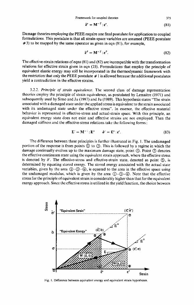
The difference between these principles is further illustrated in Fig. 1. The undamaged portion of the response is from points @ to 0. This is followed by a regime in which the damage continually evolves up to the maximum damage state, point 0. Point @ denotes the effective continuum state using the equivalent strain approach, where the effective stress is denoted by 6’. The effective-stress and effective-strain state, denoted as point 0, is determined by equating stored energy. The stored energy associated with the actual state variables, given by the area (i-O-8, is equated to the area in the effective space using the undamaged modulus, which is given by the area @-Q-0. Note that the effective stress for the principle of equivalent strain is considerably higher than that for the equivalent energy approach. Since the effective stress is utilized in the yield function, the choice between
3
4 A, Q
t
“Equivalent Strain” Eb) .---..___-____________________.________.------------.-------~~______,
*‘:O .*’ : .’ - I’ i
Fig. I. Difference between equivalent energy and equivalent strain hypotheses.
376 N. R. HANSEN and H. L. SCHKEYEK
the principle of equivalent energy and principle of equivalent strain has a marked difference on the behavior of the model.
In summary, two popular phenomenological hypotheses employed by various damage representation theories have been evaluated relative to their applicability to the derived thermodynamic framework. Additional postulates to determine the effective strains were shown to be at variance with the effective strains given in Section 2.2.2. based on the form of the dissipation rate. Therefore, for the present thermodynamic framework, the relations for the effective strains are a consequence of the form of the dissipation rate and may not be postulated or derived separately.
In the next subsections, three specific damage formulations are presented and evaluated using the general framework. The principle of equivalent elastic energy with the restrictions as discussed in Section 3.2.1 is employed for the specific formulations. A similar set, with similar results, could be developed using the principle of equivalent strains, but are not presented. All three damage formulations are found in the literature and have been developed using a phenomenological approach to damage representation. First, a simple scalar isotropic formulation is considered. Then a second-order anisotropic damage theory is evaluated. Finally, a class of damage models where the damage measure is directly associated with the damaged stiffness tensor is formulated; hence, this is a fourth-order anisotropic damage theory. Due to their phenomenological origins, each of these for- mulations is shown to possess deficiencies.
3.2.3. Sculur isotropic damage. Isotropic scalar damage theories are the most common models found in the literature. The scalar variable, d, represents the amount of volumetric material damage. The effective stress is postulated to be of the form :
With the use of the principle of equivalent elastic energy, the damaged stiffness relation is :
E = (1 -d)‘E”. (85)
The thermodynamic damage variable is selected as d and all other damage related variables are scalars. For easy comparison with other models, neglect the surface energy contribution to the Helmholtz function and the damaging shift variable. The damage energy release rate, y, or the variable conjugate to the thermodynamic damage is :
y = (l-d)C:EO:C. (86)
Recall that the damage function is constructed using HOD0 functions. For scalar damage variables, the damage function degenerates to the following :
%LY,y”) = y-(yH+Q) d 0. (87)
The resulting evolution relations and a postulated constitutive relation for yH(dH) are :
d=l* J” = -&, y” E -ti,,d”, (88)
where ti,, is a scalar material parameter. Only two material parameters, o,, and K, are required for this formulation. The inability to model the anisotropy associated with damage is the major weakness of isotropic theories. As shown by Ju (1990) an isotropic damage model implies that the Poisson’s ratio does not change, a feature at variance with some experimental data. In addition, compressive and tensile loads cannot be differentiated. Hence, equal damage states would be predicted for uniaxial tension and compression load
Framework for coupled theories 311
paths of the same magnitude. A hydrostatic pressure dependence in the damage function could be incorporated to differentiate between tension and compression in some sense but this would not be sufficiently general to properly represent all load paths. These deficiencies render scalar theories ineffective for the modeling of some materials.
3.2.4. Second-order damage measure. In this section, an anisotropic damaged-elasticity theory initially proposed by Cordebois and Sidoroff (1979) is considered. This has since been used in one form or another by several investigators including Chow and Wang (1987a, b). First, introduce a second-order symmetric damage tensor, D. A symmetric second-order tensor as the damage measure implies that the most complicated anisotropy that can be represented is orthotropic, a rectangular symmetry with axis aligned with the principal basis of the damage tensor. This orthotropy is not fixed in the material but the orthotropy rotates with the principal basis of the damage tensor. From a micromechanical derivation, Kachanov (1987) showed that even for high crack densities with interacting cracks, the effective elastic properties remained orthotropic with good accuracy. Therefore, this limi- tation on the type of anisotropy does not appear to be too restrictive.
Cordebois and Sidoroff (1979) postulated the effective stress to be of the form :
& = (i-D)~“2.a.(i-D)~‘~2 E M(D):u (89)
which also defines the fourth-order effective-stress operator M(D) as :
Mijk[ = (6i~-Di~)‘~‘(6j,-Oj,)“‘. (90)
By employing the principle of elastic energy equivalence the damaged stiffness tensor is :
where the symmetry of the damage tensor causes E to possess all the symmetries of E”. The logical choice for the thermodynamic damage variable is the second-order damage
measure, D. The damage energy release rate associated with this selection is :
(92)
where
IR = (i-D)“2. (93)
Unfortunately, a thorough evaluation reveals that Y is nor a symmetric second-order tensor unless the damage and the strain tensors have the same principal bases. A damage tensor which is nonsymmetric is a direct violation of the assumed symmetry for D. A simple change in the selection of the thermodynamic variable will remedy this dilemma. Instead of D, let L! be the thermodynamic damage variable. Physically, R is more of a measure of the material integrity than a measure of the damage, but the selection as a thermodynamic damage measure is allowable. The following consequences hold :
D =OD=!&R’)~ =i. 1=0 t=0
(94)
By taking advantage of the symmetry of the individual tensors and noting that 8, = E~ikiklRk,,,~,,,,,Q,Znl, the damage energy release rate, Y, associated with Q is given by :
SAS 31:3-6

378 N. R. HANSEN and H. L. SCHREYEK
Y =-~~-(B.R.s’+e’.R.~)+2y,(D.*+R.D). (95)
The credibility of the damage function is based on how well it correlates with exper- imental observations. Consider some observed phenomena in brittle materials. Exper- imentally, it is observed in uniaxial tension that the microcracks develop perpendicular to the loading direction or the damage is in the direction of loading. Therefore, in uniaxial tension the damage evolves in the direction of tensile stress and tensile strain. Conversely, in an unconfined uniaxial compressive stress state, the microcracks develop in the direction parallel to the loading axis. This then corresponds to damage perpendicular to the direction of loading. No stresses are present in this off-axis direction in uniaxial compression but the Poisson effect produces tensile strains in the off-axis direction. Based on these observations it appears reasonable, to postulate that damage evolves in the direction of tensile strains. Define a fourth-order projection operator, P+, such that only the tensile strain components of E are extracted :
E+ SP+:&. (96)
This projection operator can be constructed by following a procedure introduced by Ju (1989). The proposed projection operator is constructed in a series of steps as outlined below. First consider the spectral decomposition of the strain tensor.
E = i E,(Pi O Pi), i= I
(97)
where si is the ith principal strain, the unit vector pi is the corresponding ith principal strain direction (or eigenvalue and eigenvector of&). The positive (tensile) spectral tensor is defined as :
Q’ - i h(&i)(pi 8 pi), i= I
in which h( ) is the Heaviside function. The positive projection operator (a fourth-order tensor) is then defined as :
P&E Q;Q;. (99)
By inspection, if all eigenvalues of E are negative (compressive) then P+ will be the null tensor and, conversely, if all eigenvalues are positive (tensile) then P+ corresponds to the fourth-order identity. The various combinations of positive and negative eigenvalues pro- jects or annihilates the appropriate components of a second-order tensor in the cor- responding principal directions of E.
For both functions, 4,,(Y, Y”) and 4D2(Y”), it is proposed that the quadratic form of a HOD0 function be employed where the tensile strain operator is used in place of the positive semi-definite tensor A. The damage function can then be expressed as :
@,(Y,YS,Y”) 3 J(Y-Y"):p+ :(Y-YS)-(JyH:P+ :YH+m,) < 0. (100)
The anisotropic nature of the problem is preserved due to the directional dependence of the projection operator and the anisotropy of the damage variables. From eqn (37), the damage (or integrity in this case) evolution is :
* = j Pf : (Y-Y”)
“n 4”,(Y,YS) (101)
Due to the negative sign in eqn (95), as the damage evolves the eigenvalues of Cl
Framework for coupled theories 319
decrease, which is equivalent to an increase in the eigenvalues of D according to eqn (94). Hence, the damage does evolve in the direction of the tensile strain projection of the damage energy release rate, as intended. The evolution relations for the damaging variables are :
(102)
If the initial value of YH = 0 then DH will remain zero. Therefore, a nonzero initial value must be assumed in order to get the evolutionary process started. An appropriate choice might be an initial isotropic value such as YH = li where r is a “small” constant.
The constitutive relations for the damaging variables must be constructed to complete this formulation. Unlike plasticity theories where isotropic hardening is often representative of the observed phenomenon, damage is generally observed to be anisotropic. As a con- sequence the scalar degeneration of the damaging variables Y” and D” would not be appropriate. A linear, but rather general, constitutive relationship could be postulated of the form :
YH(DH) = -G : D” (103)
where C is a fourth-order tensor to be specified. In the absence of experimental data, simpler relationships for the damaging variables are postulated of the form :
Y”(D”) 3 -u,D", YS(Ds) E -IQD’ (104)
where K,, and IQ. are positive scalar material parameters. Consider the case where 6, Q and E all have the same principle bases and examine the
damage energy release rate of eqn (95). Under a uniaxial tensile stress load path, the tensile strains are in the direction of the tensile stress, while in the off-axis direction the stresses are zero. Hence, the only nonzero component of Y is in the direction of the loading. This produces damage evolution in this direction as was intended. A further evaluation of Y reveals some problems. For the load path of uniaxial compression stress, the only nonzero component of Y is again along the loading axis by the same arguments but the strains are compressive in the loading direction. The positive strain projection operator eliminates components in the direction of negative strains and hence no damage evolution is predicted for uniaxial compression. This is the first deficiency for this formulation.
The second is illustrated by considering a triaxial compression load path. For sufficient axial loading, the strains in the directions of the confining pressure will eventually become positive due to the Poisson effect from the axial load. The difference in signs between the stresses and the strains in the off-axis direction causes Y to have positive eigenvalues which then causes the principle values of R to increase, which implies a decrease in the principle values of the damage. A decrease in damage is the same as “healing” of the material which is not allowed based on physical considerations. This condition can be remedied by redefining the positive projection operator used in the damage function with one that is based on both tensile strains and stresses. For this modification, no damage evolution is predicted for the triaxial compression load path.
A remedy to the first deficiency does not follow as easily. Basically, there are two areas that can be modified in the preceding formulations. A new form of the Helmholtz thermodynamic potential could be postulated and/or a new damage function could be constructed. No satisfactory resolution to the above dilemma has been obtained. For tensile loading conditions, the formulation does well, however, for compressive type loading this formulation appears to be deficient. The inability to predict lateral damage due to an unconfined compression results from the form of the damage energy release rate which is actually a consequence of the damage representation theory as postulated by Cordebois
380 N. R. HANSEN and H. L. SCHIUXH
and Sidoroff (1979). This model is a simple approximation to damage based on volume averages of the effective-areas which does not contain sufficient detail to predict the complex mechanisms occurring on the sub-scale. Until a refined damage representation theory is employed, this is probably the best that can be expected from this formulation.
3.2.5. Fourth-order dumup meusure. A class of anisotropic damage theories is cvalu- ated in which the damaged stiffness tensor evolves directly. This approach has been followed
by a number of researchers, including Simo and Ju (1987), Ju (1989), and Yazdani and Schreyer (1990). The thermodynamic damage variable is taken to be the damaged stiffness tensor, E. Since the damage variable is a fourth-order tensor, all damaging variables are assumed to be fourth-order tensors. The damaging variable associated with shift and the
surface energy term are neglected for comparison with the formulations of others. The
fourth-order damage energy release rate, Y, is given by :
y = -,-I(E(.OEC). (105)
A damage function based on tensile strain projection is again postulated :
@,,(Y,Y”) = JY-rIP- ::Y-(JY”::p+ ::YHfq,) 6 0, (106)
where P+ is now an eighth-order tensor. The damaged stiffness evolution is then :
(107)
The components of the damaged stiffness tensor are degraded corresponding to the
directions of principal tensile strains, which correlates to the observations in brittle materials. However, this fourth-order theory also contains inherent deficiencies. Consider
a uniaxial tensile load path, where the specimen is taken to the state of significant damage. Now release the load and reload in pure shear. The previous degradation of the stiffness tensor leaves the shear components of the damaged stiffness tensor unaltered, and hence, a shear loading responds as an undamaged material. This may not be physically realistic.
The preceding approach is formulated independent of an effective-stress relation.
Recall that the effective-stress relation is the crucial mechanism by which the effective-stress plasticity and damage theories are coupled. Therefore, to calculate the effective stresses, the operator, M, must be extracted from the evolved damaged stiffness tensor. A method for performing this extraction is outlined below. For any damage representation where the principle of equivalent elastic energy is employed, the damaged stiffness is related to the effective-stress operator by :
E=M-‘:E”:M-T. (108)
Next perform a Cholesky decomposition of the damaged and undamaged stiffness tensors :
E=G:GT, E” = H: HT. (109)
These results can be combined to obtain a relation for the effective-stress operator :
G:Gr = Mp’:(H:HT):Mm7>M-’ = G:H-‘. (110)
For plausible evolutions of the stiffness tensor, the effective-stress operator that is extracted using eqn (110) does not always produce a symmetric effective-stress tensor, a result which may not be physically plausible. In addition, the computational effort required to perform this decomposition is extensive and considering that at least one decomposition
Framework for coupled theories 381
would be required for each load step, the practical utility of this approach becomes cost prohibitive. The difficulty in extracting the effective-stress operator may render this approach ineffective for a coupled formulation.
An alternate fourth-order approach which does not require a Cholesky decomposition of the stiffness tensor is proposed. Introduce a fourth-order damage tensor, D, and unlike the previous fourth-order theory which used E, this tensor is also the thermodynamic damage variable. The damage tensor is required to possess the symmetries D,ik, = Dklii = Diik, = D,,. An effective-stress relation is postulated to be of the form :
& 3 (I-D)-’ :o, (111)
where I is the fourth-order identity tensor. This also provides the definition for the effective- stress operator which is M = (I-D)- ‘. Then with the principle of equivalent elastic energy the damaged stiffness is :
E = (I-D):E”:(I-D). (112)
This implies a damage energy release rate of the form :
Y = ~[ci@&‘+&“@i+]. (113)
The damage function is that given in eqn (106) and the resulting damage evolution is :
P+:Y D = h4D,(y). (114)
The problem associated with the extraction of the effective-stress operator is thus avoided using this approach. The effective-stress operator is constructed using the damage tensor as it evolves. Unfortunately, the inability to predict the observed evolution of lateral damage from unconfined compression is exhibited, similar to the results associated with the use of a second-order damage tensor. The problem related to the undamaged shear components of the stiffness tensor, as discussed for the previous fourth-order theory, is again exhibited. Although this fourth-order theory can now be utilized in a coupled formulation because a relation for the effective stress is available, some deficiencies are still apparent. In summary, each of the three phenomenological damage formulations possess an inherent deficiency that results from approximation of the complex microscale mechanisms.
3.3. Specific coupled models The utility of the thermodynamically consistent framework developed in Section 2 is
highlighted when considering specific coupled models. A coupled formulation is thermo- dynamically consistent if both the elastoplasticity and the damage portions are developed using the framework such as those presented in Sections 3.1 and 3.2, respectively. Therefore, any of the specific plasticity models presented in Section 3.1., or others developed in a similar manner, can be coupled without further derivations to any specific damage model such as those given in Section 3.2.
To illustrate the ease by which different elastoplasticity and damage formulations can be coupled, a specific example is presented. For the elastoplasticity model, the JZ plasticity model with linear isotropic hardening and linear kinematic (Prager) hardening is selected. The damage model selected is the damage representation theory of Cordebois and Sidoroff (1979) with the anisotropic damage function based on tensile strain projections, as presented in Section 3.2.2. Using these specific models, the pertinent relations for the coupled for- mulation are summarized as follows :
Damage energy release rate :
Y = -f(O.n.~~+~~.R.6)+2y~(D.n+n.D)
382
Damage function :
N. R. HANSEN and H. L. SCHREYEH
@,(Y, YS, YH) = Jjy-yv+ : (Y-Y”) -(JT~~~+wu) < 0
Damage evolution relations :
Damaging constitutive relations :
Damage :
YH(DH) = -K,D~, YS(DS) z - rckDS
D = i-n2
Damaged stiffness :
Yield function :
ap(ii,P,6H) = J(O-ii”)“: (6-OS)“-(ci”+r7i,.) < 0
Plasticity evolutions relations :
$P =I 1, (&cis)d
(&@)d: (&@)J 6” = -p, pf = -.I,
Hardening constitutive relations :
&“(a”) 3 -K&P, c?“(P) E -Kp
Effective strain rate mapping :
ip = M(D) : 4’.
In addition to the undamaged elasticity parameters, the number of material parameters required for this coupled formulation is at most seven: (yo, wO, K,, IQ, CJ),, K,, K,), while the minimum required is four material parameters (oO, K,,, CT,., K,).
4. SPECIFIC APPLICATIONS
Most metals behave in a ductile manner, which is typically represented by plasticity models, although given sufficient load metals will eventually damage and break. Therefore, both plastic and damage processes occur, and hence, a coupled formulation is needed. To demonstrate the applicability of coupled formulations to ductile failure, a method of evaluating the individual mechanisms must be established. As part of the experimental procedure, a technique for the direct measurement of the damage is required. Other than fatigue damage, little experimental effort has been dedicated to the investigation of the damage in ductile materials such as metals.
The term “direct” measurement does not imply that the size, distribution, and orien- tations of the microcracks are measured throughout a test. Instead, the state of the material integrity is determined in an averaged sense by easily measured parameters. For example, the change in elastic modulus, which is an explicit function of the damage state, is the direct damage measurement employed by Cordebois and Sidoroff (1979), Chow and Wang (1987b), and Lemaitre (1983). Elastic unloading at periodic intervals in the test sequence is used to determine the changes in the elastic modulus. This approach is in contrast to other investigators that correlate a material state parameter just prior to rupture as a

Framework for coupled theories 383
measure of damage. For example, a measure of the plastic-strain is sometimes used to infer the failure. This is an example of an indirect measure of damage.
At least for some materials, the damage process appears to only occur in the post-peak or softening regime of the stress-strain response. In this response regime, a specimen may separate or localize into two distinct material domains. In a relatively small region as the load (strain) increases the material cannot sustain the previous value of stress because of damage, a feature often called material softening. It is within this localized zone that extensive amounts of damage occur. The remaining material that surrounds the localized zone unloads without further plastic flow or damage. The determination of how the localized region is established and the evolution of the region is still a very active research area. A completely satisfactory method for experimentally evaluating the damaging process as it occurs within the localized zone has yet to be established.
Once a material localizes or softens the boundary value problem becomes ill-posed as exhibited by lack of convergence with mesh refinement for numerical solutions. Some researchers, e.g. Chen and Schreyer (1990) and Bazant (1990), have proposed nonlocal approaches as a means of circumventing these problems. This particular subject was not a part of this research. For now, assume that the materials data considered in this section are correct for a representative volume element and that it is understood that an incorporation into the constitutive formulation of softening requires an additional feature such as nonlocal terms.
4. I. Aluminum alloy 2024 Fortunately, all three sets of data provided by Cordebois and Sidoroff (1979), Chow
and Wang (1987b), and Lemaitre (1983) contain results for the aluminum alloy 2024. These are the data to be considered for comparison with the models. Chow and Wang (1987b) indicated the alloy temper as 2024-T3 but the others did not specify the temper. Results are similar using independent testing techniques ; thus, either the tempers were the same, or the temper had little effect on the results. The first explanation is the most probable.
Unfortunately, all the authors presented incomplete descriptions of the test setup and results. All samples were tested using a load path of uniaxial tensile stress. Chow and Wang (1987b) used sheet stock aluminum in a “dog-bone” shape. The samples were marked with reference lines for inferring strains. Lemaitre (1983) conducted tests using cylindrical tensile bars, and the material strains were measured using small (0.5 mm) strain gages. Cordebois and Sidoroff (1979) did not describe their test setup. It is assumed that all tests were conducted at room temperature. With respect to the test results, none of the researchers presented a corresponding stress-strain response, but all provided results relative to the damage evolution (either a damage measure or the change in the elastic modulus). Chow and Wang (1987b), along with Cordebois and Sidoroff (1979), also presented results on the evolution of the lateral strains which is used to determine the apparent Poisson’s ratio. None indicated whether or not a zone of localization appeared.
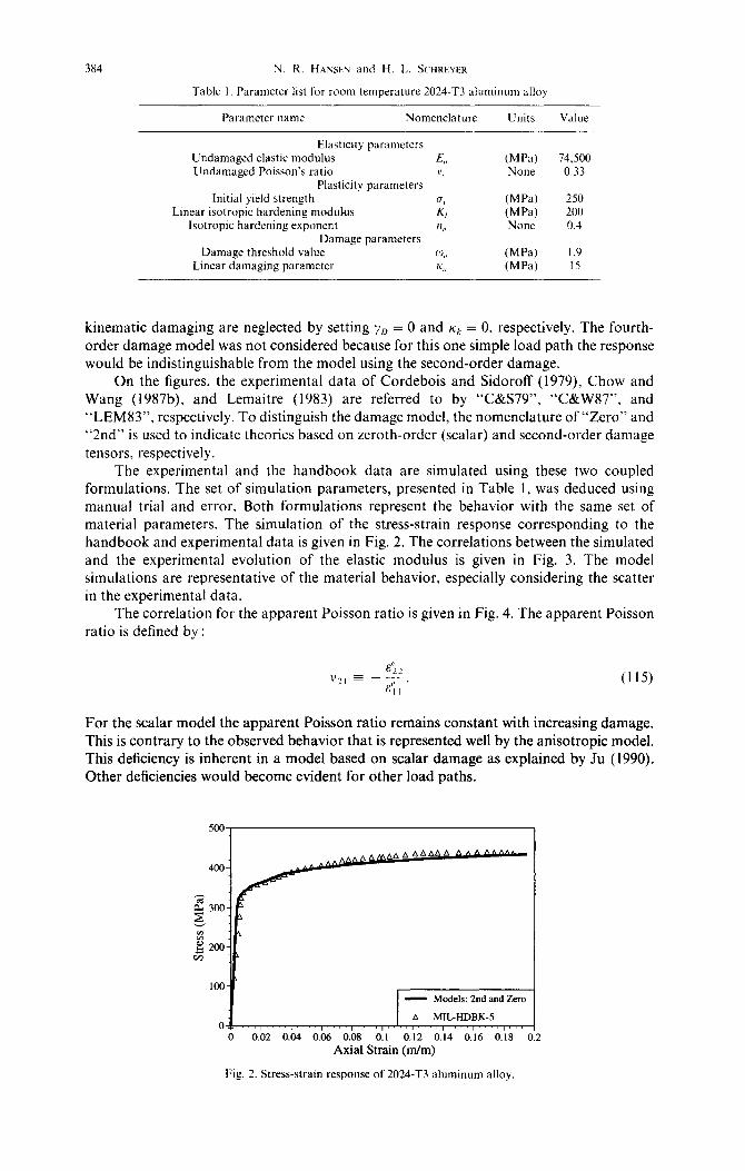
Since no stress-strain data were provided, typical full-range stress-strain response data for 2024-T3 aluminum alloy were taken from a standard metals handbook (MIL-HDBK- 5E, 1987). A slight inconsistency between the handbook and the experimental data was observed. The maximum strain from the handbook was approximately 0.19, while the experimental results indicated maximum strains of at least 0.25. It is assumed that the experimental results up to a strain value of 0.19 are consistent with the handbook data.
Two different coupled formulations are used to simulate the experimental data. The J2 plasticity model of Section 3.1. with isotropic hardening is used for both coupled formulations. The nonlinear hardening relation ofeqn (73) is employed because it represents the shape of the hardening response for this alloy better than the linear relation. No kinematic hardening is incorporated since the load path is strictly monotonically increasing. The difference between the two coupled formulations is the damage portion of the model. The scalar isotropic damage model of Section 3.2.1. and the second-order damage model of Section 3.2.2. are considered. The latter is identical to the coupled formulation sum- marized in Section 3.2.3. with the inclusion of the nonlinear isotropic hardening. For both of the damage models the surface energy contribution to the Helmholtz function and the
384 %. R. HANSEN and H. L. SCwww
Table I. Parameter list for room temperature 2024-T3 aluminum alloy
Parameter name Nomenclature Units Value
Elasticity parameters Undamaged elastic modulus 6, (MPa) 74.500 Undamaged Poisson’s ratio “,a None 0.33
Plasticity parameters Initial yield strength
2, (MI%) 250
Linear isotropic hardening modulus (MPd) 200 Isotropic hardening exponent % None 0.4
Damage parameters Damage threshold value (‘J,, (MPa) 1.9
Linear damaging parameter K,, (h’if’d) 15
kinematic damaging are neglected by setting y. = 0 and IQ = 0, respectively. The fourth- order damage model was not considered because for this one simple load path the response would be indistinguishable from the model using the second-order damage.
On the figures. the experimental data of Cordebois and Sidoroff (1979), Chow and Wang (1987b), and Lemaitre (1983) are referred to by “C&S79”, “C&W87”. and “LEM83”, respectively. To distinguish the damage model, the nomenclature of “Zero” and “2nd” is used to indicate theories based on zeroth-order (scalar) and second-order damage tensors, respectively.
The experimental and the handbook data are simulated using these two coupled formulations. The set of simulation parameters, presented in Table 1, was deduced using manual trial and error. Both formulations represent the behavior with the same set of material parameters. The simulation of the stress-strain response corresponding to the handbook and experimental data is given in Fig. 2. The correlations between the simulated and the experimental evolution of the elastic modulus is given in Fig. 3. The model simulations are representative of the material behavior, especially considering the scatter in the experimental data.
The correlation for the apparent Poisson ratio is given in Fig. 4. The apparent Poisson ratio is defined by :
For the scalar model the apparent Poisson ratio remains constant with increasing damage. This is contrary to the observed behavior that is represented well by the anisotropic model. This deficiency is inherent in a model based on scalar damage as explained by Ju (1990). Other deficiencies would become evident for other load paths.
0 0 0.02 0.04 0.06 0.08 0.1 0.12 0.14 0.16 0.18 (
Axial Strain (m/m)
Fig. 2. Stress-strain response of 2024-T3 aluminum alloy.
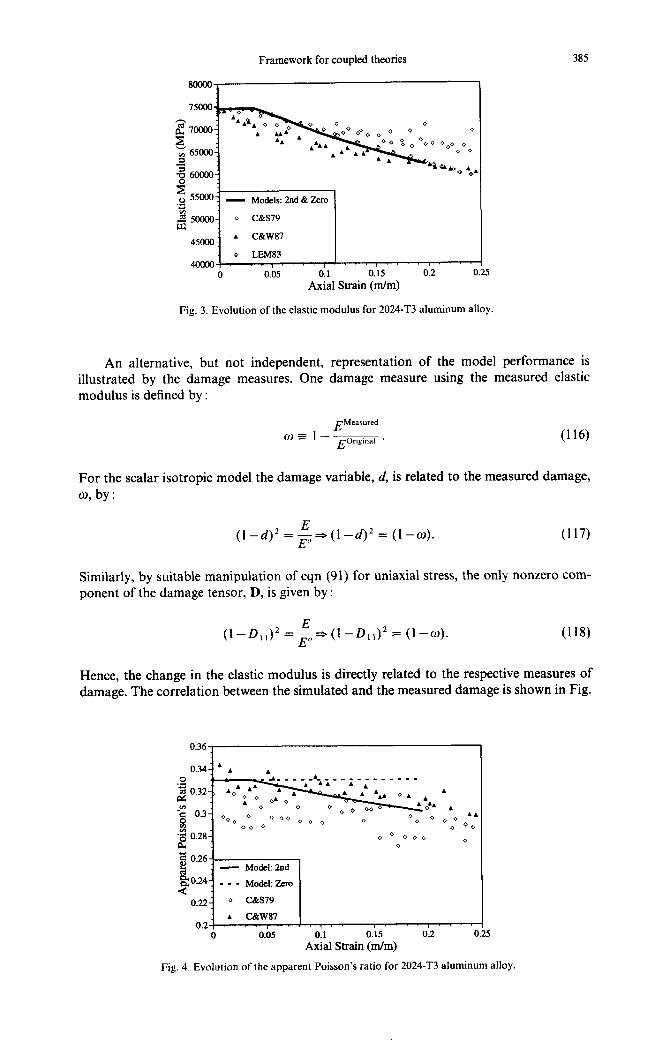
Framework for coupled theories 385
0 0.05 0.1 0.15 0.2 0 Axial Strain (m/m)
?5
Fig. 3. Evolution of the elastic modulus for 2024-T3 aluminum alloy.
An alternative, but not independent, representation of the model performance is illustrated by the damage measures. One damage measure using the measured elastic modulus is defined by :
EMeasured
fJj_ I---- Eoriplnal . (116)
For the scalar isotropic model the damage variable, d, is related to the measured damage, w, by:
(l-d)2 =&l-d)* =(1-o). (117)
Similarly, by suitable manipulation of eqn (91) for uniaxial stress, the only nonzero com- ponent of the damage tensor, D, is given by :
(l-D,,)* +(1-D,,)*= (1-w). (118)
Hence, the change in the elastic modulus is directly related to the respective measures of damage. The correlation between the simulated and the measured damage is shown in Fig.
0.36
a
3 0.26 2 : - Model: 2nd
gO.24: _ _ _ Model: k <
0.22: 0 C&S79
: L C&W87 0.2 I, ” I ” ” I ” ” I.“’
0 0.05 0.1 0.15 0.2 0
Axial Strain (m/m) .5
Fig. 4. Evolution of the apparent Poisson’s ratio for 2024-T3 aluminum alloy.
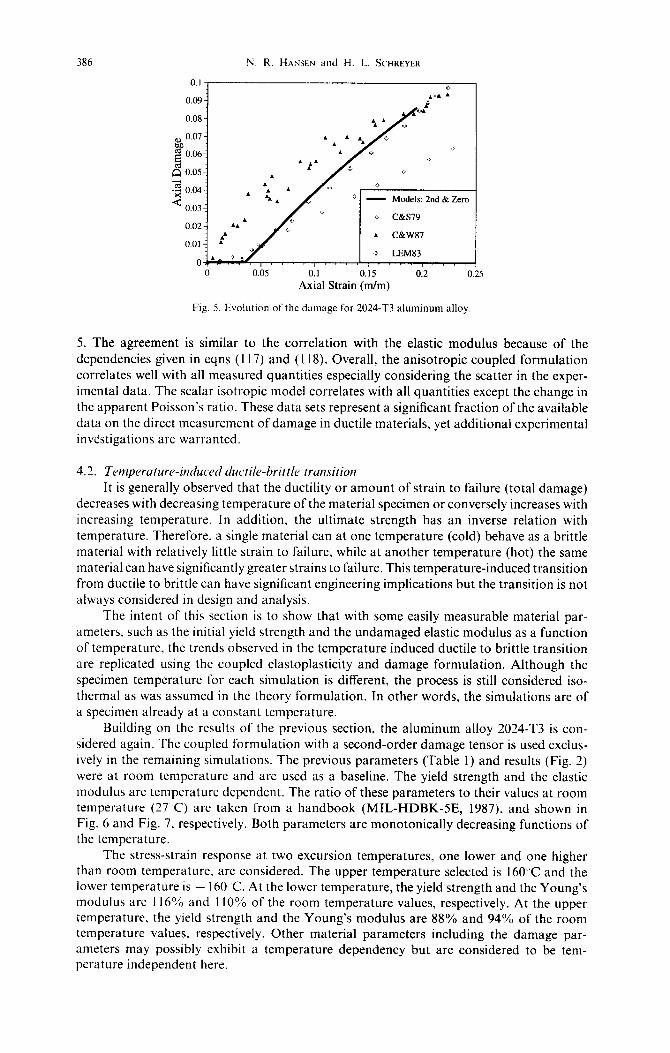
386 N. R. HANSEN and H. L. SCHKEYCK
- Models: 2nd &Zero
0 C&S19
0 0.05 0.1 0.15 0.2 0
Axial Strain (m/m)
Fig. 5. Evolution of the damage for 2024-T3 aluminum alloy.
!5
5. The agreement is similar to the correlation with the elastic modulus because of the
dependencies given in eqns (117) and (118). Overall, the anisotropic coupled formulation correlates well with all measured quantities especially considering the scatter in the exper- imental data. The scalar isotropic model correlates with all quantities except the change in the apparent Poisson’s ratio. These data sets represent a significant fraction of the available data on the direct measurement of damage in ductile materials, yet additional experimental investigations are warranted.
4.2. Temperature-induced duc~tile4wittl~ transition
It is generally observed that the ductility or amount of strain to failure (total damage) decreases with decreasing temperature of the material specimen or conversely increases with increasing temperature. In addition, the ultimate strength has an inverse relation with temperature. Therefore. a single material can at one temperature (cold) behave as a brittle
material with relatively little strain to failure, while at another temperature (hot) the same material can have significantly greater strains to failure. This temperature-induced transition from ductile to brittle can have significant engineering implications but the transition is not
always considered in design and analysis.
The intent of this section is to show that with some easily measurable material par- ameters, such as the initial yield strength and the undamaged elastic modulus as a function of temperature, the trends observed in the temperature induced ductile to brittle transition are replicated using the coupled elastoplasticity and damage formulation. Although the specimen temperature for each simulation is different, the process is still considered iso-
thermal as was assumed in the theory formulation. In other words, the simulations are of a specimen already at a constant temperature.
Building on the results of the previous section, the aluminum alloy 2024-T3 is con- sidered again. The coupled formulation with a second-order damage tensor is used exclus- ively in the remaining simulations. The previous parameters (Table 1) and results (Fig. 2) were at room temperature and are used as a baseline. The yield strength and the elastic
modulus arc tcmpcraturc dcpcndent. The ratio of these parameters to their values at room temperature (27-C) are taken from a handbook (MIL-HDBK-SE, 1987). and shown in Fig. 6 and Fig. 7, respectively. Both parameters are monotonically decreasing functions of the temperature.
The stress-strain response at two excursion temperatures, one lower and one higher than room temperature, are considered. The upper temperature selected is 160 ‘C and the lower temperature is - 160 C. At the lower temperature, the yield strength and the Young’s modulus are I 16% and I 10% of the room temperature values, respectively. At the upper temperature, the yield strength and the Young’s modulus are 88% and 94% of the room temperature values, respectively. Other material parameters including the damage par- ameters may possibly exhibit a temperature dependency but are considered to be tem- perature independent here.
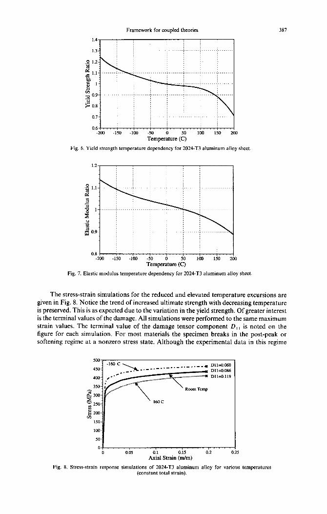
Framework for coupled theories
Temperature (C)
Fig. 6. Yield strength temperature dependency for 2024-T3 aluminum alloy sheet.
1.2
.gi 1.1
d
2
$1
5: .Y
2 n 0.9
0.8 -200 -150 -100 -50 0
Temperature ($ 100 150 0
Fig. 7. Elastic modulus temperature dependency for 2024-T3 aluminum alloy sheet.
387
The stress-strain simulations for the reduced and elevated temperature excursions are given in Fig. 8. Notice the trend of increased ultimate strength with decreasing temperature is preserved. This is as expected due to the variation in the yield strength. Of greater interest is the terminal values of the damage. All simulations were performed to the same maximum strain values. The terminal value of the damage tensor component D, , is noted on the figure for each simulation. For most materials the specimen breaks in the post-peak or softening regime at a nonzero stress state. Although the experimental data in this regime
500
450
400
350
23300 5: - 250 3 g 200 WI
150
loc
50
a
__.__._ .._-. -..--4l Dll=O.O60 v Dll=O.086
Dll=OJ19
0:1 o.i5 0:2 C Axial Strain (m/m)
25
Fig. 8. Stress-strain response simulations of 2024-T3 aluminum alloy for various temperatures (constant total strain).
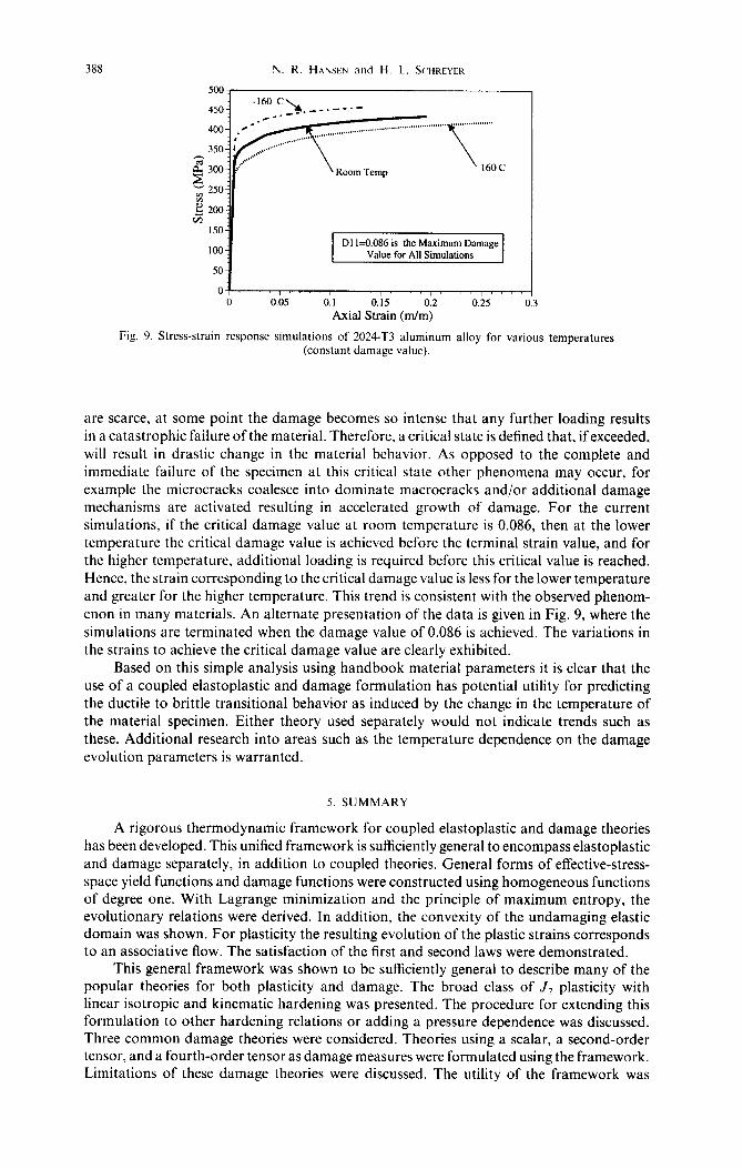
388 N. R. HA~~SEN and H. L. %‘HKEYFK
loo D11=0.086 is the Maximum Damage
Value for All Simulations
‘11 0 0.05 0.1 0.15 0.2 0.25
Axial Strain (m/m)
Fig. 9. Stress-strain response simulations of 2024-T3 aluminum alloy for various temperatures (constant damage value).
are scarce, at some point the damage becomes so intense that any further loading results in a catastrophic failure of the material. Therefore, a critical state is defined that, if exceeded, will result in drastic change in the material behavior. As opposed to the complete and immediate failure of the specimen at this critical state other phenomena may occur, for example the microcracks coalesce into dominate macrocracks and/or additional damage mechanisms are activated resulting in accelerated growth of damage. For the current simulations, if the critical damage value at room temperature is 0.086, then at the lower temperature the critical damage value is achieved before the terminal strain value, and for the higher temperature, additional loading is required before this critical value is reached. Hence, the strain corresponding to the critical damage value is less for the lower temperature and greater for the higher temperature. This trend is consistent with the observed phenom- enon in many materials. An alternate presentation of the data is given in Fig. 9, where the simulations are terminated when the damage value of 0.086 is achieved. The variations in the strains to achieve the critical damage value are clearly exhibited.
Based on this simple analysis using handbook material parameters it is clear that the use of a coupled elastoplastic and damage formulation has potential utility for predicting the ductile to brittle transitional behavior as induced by the change in the temperature of the material specimen. Either theory used separately would not indicate trends such as these. Additional research into areas such as the temperature dependence on the damage evolution parameters is warranted.
5. SUMMARY
A rigorous thermodynamic framework for coupled elastoplastic and damage theories has been developed. This unified framework is sufficiently general to encompass elastoplastic and damage separately, in addition to coupled theories. General forms of effective-stress- space yield functions and damage functions were constructed using homogeneous functions of degree one. With Lagrange minimization and the principle of maximum entropy, the evolutionary relations were derived. In addition, the convexity of the undamaging elastic domain was shown. For plasticity the resulting evolution of the plastic strains corresponds to an associative flow. The satisfaction of the first and second laws were demonstrated.
This general framework was shown to be sufficiently general to describe many of the popular theories for both plasticity and damage. The broad class of J2 plasticity with linear isotropic and kinematic hardening was presented. The procedure for extending this formulation to other hardening relations or adding a pressure dependence was discussed. Three common damage theories were considered. Theories using a scalar, a second-order tensor, and a fourth-order tensor as damage measures were formulated using the framework. Limitations of these damage theories were discussed. The utility of the framework was

Framework for coupled theories 389
demonstrated by formulating a coupled model using the specific elastoplasticity and damage models.
Two coupled formulations involving scalar isotropic damage and the second-order anisotropic damage were then used to replicate the experimental data for 2024-T3 aluminum alloy. The anisotropic formulation was shown to replicate all of the observed behavior. As expected, the scalar isotropic model did not correlate well with data exhibiting a change in the apparent Poisson ratio. In addition, the observed trends for temperature induced ductile- to-brittle transition was replicated using easily measured material parameters.
Acknowledgement,s-This work was supported by the U.S. Department of Energy under Contract DE-ACO4- 76DPOO789. This paper is based in part on the first author’s Ph.D. dissertation.
REFERENCES
Bazant, Z. P. (1990). Recent advances in failure localization and nonlocal models. In Micromechanics of Failure of Quasi-Brittle Materials (Edited by S. P. Shah, S. E. Swartz and M. L. Wang), pp. 12-37. Elsevier, Amsterdam.
Callen, H. B. (1985). Thermodynamics and an Introduction to Thermostatistics. Wiley, New York. Chen, Z. and Schreyer, H. L. (1990). Failure-controlled solution strategies for damage softening with localization.
In Micromechanics of Failure of Quasi-Brittle Materials (Edited by S. P. Shah, S. E. Swartz and M. L. Wang), pp. 135-145. Elsevier, Amsterdam.
Chow, C. L. and Wang, J. (1987a). An anisotropic theory of continuum damage mechanics for ductile fracture. Engn,q Fract. Mech. 27, 547-558.
Chow, C. L. and Wang, J. (1987b). An anisotropic theory of elasticity for continuum damage mechanics. ht. J. Fracl. 33, 3-16.
Coleman, B. D. and Gurtin, M. E. (1967). Thermodynamics with internal state variables. J. Chem. Phys. 47,597- 613.
Cordebois, J. L. and Sidoroff, F. (1979). Damage Induced Elastic Anisotropy. Colloque Euromech 115, Villard de Lans. Also appearing in Boehler J. P. (eds) (1983), Mechanical Behavior of Anisotropic Solids. pp. 761-774, Martinus Nijhoff.
Davis, H. T. (1960). Introduction to Nonlinear Dijerential and Integral Equations. U.S. Atomic Energy Com- mission.
Hill, R. (1950). The Mathematical Theory of Plasticity. Oxford University Press, London. Ju, J. W. (1989). On energy-based coupled elastoplastic damage theories : constitutive modeling and computational
aspects. Int. J. Solids Structures 25, 803-833. Ju, J. W. (1990). Isotropic and anisotropic damage variables in continuum damage mechanics. J. Engng Mech.
ASCE, 116,2764-2770. Kachanar, L. M. (1958). Time of rupture process under creep conditions. IVZ Akad. Nauk, S.S.R., Otd. Tech.
Nauk 8,263 I. Krajcinovic, D. (1989). Damage mechanics. Mech. Mater. 8, 117-197. Lemaitre, J. (1971). Evaluation of dissipation and damage in metals. Proc. I.C.M., Vol. 1, Kyoto, Japan. Lemaitre, J. (1983). A continuous damage mechanics model for ductile fracture. J. Engng Mater. Tech., ASME
107,83-89. Lubliner, J. (1972). On the thermodynamic foundations of nonlinear solids mechanics. Int. J. Non-Linear Mech.
I, 237-254. Lubliner. J. (1984). A maximum-dissipation principle in generalized plasticity. Acta Mech. 52,225-237. MIL-HDBK-SE (1987). Metallic Materials and Elements for Aerospace Vehicle Structures. U.S. Department of
Defense. Simo, J. C. and Hughes, T. J. R. (1988). Plasticity and Viscoplasticity : Numerical Analysis and Computational
Aspects. Springer, Berlin. Simo, J. C. and Ju, J. W. (1987). Stress and strain based continuum damage models, parts I and II. Int. J. Solids
Structures 23,821-869. Stevens, D. J. and Liu, D. (1992). Strain based constitutive model with mixed evolution rules for concrete. J.
Engng Mech. ASCE 118, I 1841200. Strang, G. (1986). Introduction to Applied Mathematics. Wellesley-Cambridge, Wellesley, MA. Yazdani, S. and Schreyer, H. L. (1990). Combined plasticity and damage mechanics model for plain concrete. J.
Engng Mech.. ASCE 116, 1435-1450. Yazdani, S. and Karnawat, S. (1992). A constitutive theory for brittle solids with elementary coupled theory
relations. In Recent Advances in Damage Mechanics and Plasticity (Edited by J. W. Ju) ASME AMD-Vol. 132, pp. 249-263.
Ziegler, H. (1963). Some extremum principles in irreversible thermodynamics with application to continuum mechanics. In Pro,qress in Solid Mechanics, Vol. 4 (Edited by I. N. Sneddon and R. Hill), North-Holland, Amsterdam.