“A Theory of Size and Product Diversity of Marketplaces ...
73
“A Theory of Size and Product Diversity of Marketplaces with Application to the Trade Show Arena” Ani Dasgupta FTS Electronic Marketplace Gary Lilien The Pennsylvania State University Jianan Wu Tulane University ISBM Report 2-2000 Institute for the Study of Business Markets The Pennsylvania State University 402 Business Administration Building University Park, PA 16802-3004 (814) 863-2782 or (814) 863-0413 Fax
Transcript of “A Theory of Size and Product Diversity of Marketplaces ...

“A Theory of Size and Product Diversity ofMarketplaces with Application
to the Trade Show Arena”
Ani DasguptaFTS Electronic Marketplace
Gary LilienThe Pennsylvania State University
Jianan WuTulane University
ISBM Report 2-2000
Institute for the Study of Business MarketsThe Pennsylvania State University
402 Business Administration BuildingUniversity Park, PA 16802-3004
(814) 863-2782 or (814) 863-0413 Fax

1
A Theory of Size and Product Diversity of Marketplaceswith Application to the Trade Show Arena
Ani DasguptaGary L. Lilien
Jianan Wu*
Version: March 9th 2000
* Ani Dasgupta (corresponding author) is an economist and a private management consultant affiliated with FTSElectronic Marketplace. Gary Lilien is Distinguished Research Professor of Management Science, PennsylvaniaState University. Jianan Wu is Assistant Professor of Marketing, A.B. Freeman School, Tulane University. Theauthors thank The Institute for the Study of Business Markets for supporting this research and Prof. SrinathGopalakrishna of University of Missouri for his input in preparing Exhibit 1.

2
Abstract
Markets involve the exchange of information and products between buyers and sellers inmarketplaces that are created by market organizers. This paper develops a theory to explain thedifferences in the size (number of participants) and diversity (range of products displayed) acrossthese marketplaces. We assume that successful transactions require information transmissionbetween parties calling for investment in time and effort. Two key factors affect this process ofinformation interchange: diminishing marginal returns to effort, which encourages diversificationand congestion cost resulting from participant overload. We study a sequential model ofinteraction between buyers, sellers and marketplace organizers. Organizers choose the numberand nature of marketplaces to organize and set entry fees, while buyers and sellers makeparticipation and effort allocation decisions. We show that participants’ breadth of productinterest, their buying and selling intensities (i.e. how frequently they are likely to engage infuture product transactions) as well as the technological innovativeness of the industry haveimportant influences on the size and range of product diversity in the marketplace. We apply thismodel to the industrial trade show arena to explain differences in trade show types (horizontalwith broad product focus vs. vertical with narrow product focus) across industries. Empiricaltests of several propositions derived from our model provide an encouraging degree of supportfor our theory. Our analysis identifies several industries that appear to be underserved by onetype of show or the other, suggesting possible future opportunities for organizers.
Keywords: Marketplaces, Trade Shows, Product Diversity, Game Theory

3
1. Introduction
Buyers, sellers and purchase influencers exchange products and information in a wide
variety of forums, including shopping centers, supermarkets, professional meetings, exhibitions
and trade shows as well as, increasingly in electronic, on-line marketplaces. While the act of
actual exchange of products is often the ultimate interaction goal, the information exchange that
precedes the actual exchange receives much less careful study. Our goal in this paper is to show
that the process of effort and time allocation towards receiving and distributing information has
major implications for the number of marketplace participants and the diversity of product
offerings in those marketplaces.
As an example of one forum where a large proportion of the participants’ time is spent on
information exchange, consider exhibitions and trade shows. In a typical trade show attendees
spend considerable time researching the costs/benefits of current and future solutions to their
needs and exhibitors invest comparable time disseminating the costs/benefits of their proposed
solutions to prospective customers. These shows constitute an important communication and
exchange medium in the business marketplace, accounting for nearly 20% of the
communications mix dollar (Business Marketing, 1999). According to one estimate (Kotler,
1999), companies annually spend more than $15 billion on trade shows in the United States
alone; moreover, these shows generate more than $70 billion in sales annually there. Trade
shows are no less important on the global scene; for instance, in 1989 there were 169
international shows held in Germany with 124,000 exhibitors and over ten million attendees.
During the same year, 220 international shows were organized in the UK with 61,000 exhibitors
and 4.6 million attendees (Hansen, 1999).
But trade shows don’t just happen. Someone must organize them and position them in the
market, setting prices (entry fees) and communication programs to encourage exhibitors and
attendees to participate. Optimal fees should maximize the organizer’s profit by drawing the
optimal number of participants while giving the right incentives for participants: i.e., no actual
participant should make more (net) profit by staying out, and no uninterested potential
participant should make more (net) profit by participating (at those fees). But, what determines
these optimal numbers? We can develop some insights into this issue by taking a closer look at
the act of information exchange.

4
Gathering of information and its dissemination, like many other economic activities, are
likely to experience diminishing marginal returns to investment in time: after some interchange
neither a buyer nor a seller is likely to get much more out of additional interaction. Since
diminishing marginal returns encourages spreading of resources across alternatives, it would
seem that marketplaces should be filled with as many buyers and sellers as possible. However,
with more participants comes congestion, a dissipation of participants’ effort that could have
been spent in information exchange. This observation suggests that a market should be divided
up among a number of marketplaces, the size of each of which should be governed by the
tradeoff between participants’ desire for diversity and the cost of congestion.
Thus, even with only (multiple varieties of) a single product one might expect multiple
marketplaces to exist; however, additional considerations emerge when we consider a market
with multiple products. In this case, a marketplace organizer has the choice between organizing
marketplaces where all products are displayed, or he may organize trading platforms where only
a few are traded. Given this choice, what kind of product coverage should the organizer opt for?
The heterogeneity of product interests across buyers and sellers clearly is a determining factor
here, but in this paper we raise a more limited question: assuming that both buyers and sellers are
homogenous, what other factors would drive us toward narrow versus broad trading platforms?
Can we define operational variables that provide guidance for the organizers about which
marketplaces might currently be ‘too narrow’ or ‘too broad’?
To our knowledge, these issues are raised here for the first time. In the Economics of
Industrial Organization literature, product diversity (or differentiation) in markets has seen
considerable attention, following the seminal models of Hotelling (1929) in the context of
oligopoly and Dixit-Stiglitz (1977) in the context of monopolistic competition (see Beath and
Katsoulacos (1991) for an overview). However, we emphasize that the notion of product
differentiation in markets is unrelated to the notion of product diversity in marketplaces. A
market or an industry may have great product diversity and yet, each marketplace may feature a
very narrow set of products. Similarly, congestion in the product markets is a well-studied
phenomenon but usually in the context of externalities that a customer experiences in the
presence of other customers (e.g. see Reitman, 1991, and the references cited there). However, in
our framework, congestion acts through its negative impact on information transmission (and
hence matching of needs), thus affecting producers in equal measure.

5
We proceed as follows. While we have couched our discussion broadly, we focus on the
specifics of the industrial exhibition or trade show here both for concreteness and to provide an
opportunity for empirical testing. Thus, Section 2 discusses trade shows and provides some
interesting observations that we seek to understand. In Section 3 we set up our model in terms of
the interaction that takes place among three types of agents: attendees, exhibitors and show
organizers. We then specify a production function and a congestion cost function. In Section 4,
we first deal with a one-product (vertical) show, identify a plausible equilibrium and calculate
the total surplus the show generates. We then do the same for a multi-product (horizontal) show
and develop a key proposition comparing the profits from a vertical show with those from a
horizontal show. In Section 5 we develop the theory that determines the size of shows as well as
the numbers of horizontal and vertical shows that one can expect to see in an industry (and, thus,
their relative proportions). Section 6 uses this theory to study the influence of various industry
characteristics on the proportion of horizontal shows, resulting in several testable hypotheses. In
Section 7 we conduct an empirical investigation of these hypotheses, providing support for our
theory. Our analysis also develops some useful managerial guidelines by pointing out which
industries, according to our theory, are currently over or underserved by horizontal (versus
vertical) shows. Section 8 discusses the implications of our findings, model limitations and
directions for further research. A glossary lists all notations used in the text while proofs of the
propositions are available in Dasgupta, Lilien and Wu (2000) or on line at
www.smeal.psu.edu/isbm.
2. Trade Show Facts and Puzzles
One type of marketplace where the issues raised above are clearly relevant involves trade
shows or (equivalently here) industrial exhibitions. Trade shows serve as excellent conduits of
information exchange as well as selling platforms for new and upcoming products. Trade shows
have been traditionally categorized as vertical or horizontal based on market coverage
(Gopalakrishna and Lilien, 1994). Typically, a vertical show involves a narrow range of products
and attracts visitors specifically interested in those products. In contrast, a horizontal show
usually involves a much broader range of products and a more diverse audience. For example,
attendees at the Association of Operating Room Nurses show, a vertical show, are almost all
operating room nurses, and exhibitors display products that are used almost exclusively in the

6
operating room. The National Design Engineering Show is a horizontal show in which firms
demonstrate products ranging from mechanical components, electrical and electronic
components, plastics, elastomers, to CAD/CAM systems (Gopalakrishna and Williams, 1992).
Exhibit 1, prepared by Exhibit Surveys Inc., details the number of vertical shows,
horizontal shows and the proportion of horizontal shows for a number of different industries
during the period from 1985 to 1991. There appears to be no simple pattern here: why are 319 of
the 322 shows in the Communications industry vertical, 61 of the 64 shows in the Food
Processing and Distribution industry horizontal while the Chemical industry splits almost evenly
with 20 vertical and 23 horizontal shows?
Even the status of existing shows evolve, with some merging and becoming more
horizontal and others splitting into more narrow shows. For instance, Conexpo-Con/Agg '96, the
largest US trade show in the construction industry, resulted from a merger of Conexpo (owned
by Construction Industry Manufacturers Association), the largest construction show, and
Con/Agg (owned by the National Aggregates Association and the National Ready Mixed
Concrete Association), one of the premier vertical shows specializing in concrete and aggregates
in the United States. The new, horizontal show attracted more than 1250 exhibitors and 100,000
attendees, and covered 1.25 million square feet of exhibiting area, making it bigger than the last
Conexpo and Con/Agg combined1. On the other hand, Comdex, the largest (horizontal) computer
show in the US, has seen threats by key exhibitors to split and form more narrowly focused
shows2.
This diversity and structural evolution of show type has seen little academic attention.
Most trade show studies emphasize lead (or sales) generation as the key goal, providing little
motivation for the existence of horizontal shows (Gopalakrishna and William 1992,
Gopalakrishna and Lilien 1993, Gopalakrishna and Lilien 1994, Dekimpe et al. 1996). These
studies measure the performance of the show by how efficiently the show generates leads or
sales and generally assume homogeneous objectives on the parts of both exhibitors and
attendees. The studies all indicate that vertical shows outperform horizontal shows in terms of
selling efficiency, calling into question the economic rationale for horizontal shows. So, why do
1 Show Daily of Conexpo and Con/Agg, '96, page 18.2 Jim Carlton, “Comdex Complaint As Big Computer Show Opens, Key Exhibitors Grumble About Costs”, WallStreet Journal, 11/14/1994, Page A1.

7
both types of shows exist and why does the proportion of show types vary so widely across
industries?
One way to address this question is to recognize that most measures of lead generation,
being rooted to benefits taking place in the present or near future, do not capture the full
economic gains that may result from information interchange and be realized in the more distant
future. This is not a new idea; the literature has recognized the existence of these dual motives of
participants in a show. For instance, Kerin & Cron (1987) have looked at the functions of trade
shows from the exhibitors' point of view and showed that there are two categories of roles that
trade shows play: selling functions and non-selling functions. Some exhibitors have objectives
that are primarily sales oriented, such as generating leads, while others have non-sales oriented
objectives such as gathering competitive intelligence and enhancing company image. Following
Kerin and Cron’s approach, Hansen (1999) reconsidered the multidimensionality of trade show
performances. He proposed a two-dimensional framework of trade show performance: an
outcome-based dimension, which includes the sales-related activities, and a behavior-based
dimension which includes nonsales-related activities, such as information-gathering activities,
image-building activities, motivation activities, and relationship-building activities. Both papers
focus solely on exhibitors, but Hansen (1999) recognizes that this dichotomy of focus may be
relevant for attendees as well.
The above discussion seems to suggest that the alleged inefficiency of horizontal shows
is solely a result of researchers’ inability to quantify the long-run economic output of non-selling
and information-gathering activities. However, this explanation holds only if horizontal shows
experience more non-selling/information gathering activity than do their vertical counterparts.
But are there a priori reasons why a wider diversity of product in a marketplace should
necessarily be correlated with a longer time horizon for transaction of the participants? One of
the goals of this paper is to show that indeed, there are such reasons. Thus, we provide an
explanation for the observation made by several authors on the superiority of vertical shows in
terms of lead generation.
One might wonder why horizontal shows, with more products and typically larger
number of participants, will not always dominate vertical shows in terms of total surplus
generation. One reason for the absence of such a clear dominance is the differences in
organizational costs: vertical shows, appealing to a narrower audience, should cost less to
organize than a horizontal show. However, there is another factor at work: exhibitors and

8
attendees may have different interests in different product categories either because of firm or
job-responsibility differences (purchasing agents vs. R&D engineers; smaller firms vs. large
firms) or because of industry differences (Williams et al, 1994). For example, in the computer
industry, a hardware manufacturer such as Intel may focus its attention on hardware; however,
Dell, another manufacturer, in its role as an attendee, may not only be concerned about hardware
but also about the software it is considering bundling with its computers. Now, returns to effort
in a potential exchange must account for efforts expended by both parties: if attendees and
exhibitors are interested in different kinds of products, or if the range of product interests is
narrow for one group and broad for the other, a mismatch arises. The allocation of effort across
different products then becomes a strategic consideration and, in equilibrium, the total gross
surplus generated in a horizontal show may not always dominate that of a vertical show or vice
versa. Thus we posit that the proportion of horizontal shows in an industry is the result of a
complex interaction between: a) the degree of diminishing marginal returns associated with the
information interchange process, b) the extent of future transaction interests of both parties, c)
the breadth of product interests of both parties and their compatibility and d) the fixed costs
associated with organizing shows.
3. The Model Setup: Benefits and Costs of Participation
In this section we specify the sequence of events in our model, and two of its key
constructs — the function relating the time/effort investment by participants into benefits (the
production function) and a deterrent factor for markets of unmanageable size, the congestion
cost. Although our model applies beyond the trade show arena, for concreteness we will refer to
the marketplace as a ‘show’ and the two categories of participants in the marketplace as
‘attendees’ and ‘exhibitors’.
A. Timing: Our model is based on the interaction between three types of agents in the
marketplace: attendees, exhibitors (assumed homogeneous within category) and (potential)
marketplace organizer(s). We will also assume there is either one product category (X) or two
product categories (X plus Y) under consideration. The sequence of events in the model is as
follows:
1. Each (potential) organizer decides how many shows of each type to set up (X and/or Y,
vertical shows or X&Y, the horizontal show). They then invest in the fixed factors, like

9
show space, publicity and so forth that do not vary with the number of participants, for
the shows they have decided to set up. We assume that the prices of these factors will
rise as the demand for them increases.
2. Next, the organizers decide on (and announce) the fees they plan to charge attendees
and exhibitors that participate in any show they organize.
3. Then, each individual from a large pool of identical potential attendees decides which
show to attend (if at all) and each individual from a large pool of identical exhibitors
(simultaneously) decides whether to participate in that show. The organizer of a show
realizes the total of the entry fees minus his variable costs.
4. Upon arriving at a show, each attendee decides how to allocate his available effort or
time among the exhibitors present. For a horizontal show, he further decides how to
allocate effort toward particular exhibitors within different product categories.
Exhibitors make similar effort allocation decisions.
Participants see benefits in interaction through a production function and see disincentives to
interaction through a congestion cost function. We specify these functions next.
B. Production Function: A simple way to model how efforts by an attendee-exhibitor pair get
translated into the benefits they seek is to develop a production function where efforts appear as
inputs and the (expected) benefit appears as the output. Such a function should have the
following properties:
a. If effort expended by either party is zero, then no matter how much effort the other party
expends, the output (or benefit) is zero.
b. The marginal return to effort of any party is increasing in the effort expended by the other
party and
c. There are diminishing marginal returns to effort for both parties, thus giving rise to
‘variety seeking’ behavior.
A commonly used specification with these properties is the Cobb-Douglas production function:
(3.1) αλ )(1 pqvrkU −=
where U is the expected benefit to a party, k is a positive constant, r is the (common) rate of
interest used by both parties, λ is the ‘future transaction intensity factor’ of the pair, v is the net
value generated to the party per unit transaction in the exhibitor’s product, p is the effort invested
by the exhibitor, q is the effort invested by the attendee and α is a parameter that captures how

10
fast marginal returns (to joint effort) diminish. We further motivate the formulation and explain
the terms in (3.1) next.
Within a product category (X or Y), we consider each exhibitor as a producer of a
specific “brand, ” where each brand has a slightly different formulation that the attendees
unaware of are a priori. Each attendee has slightly different needs, characterized by an
idiosyncratic taste parameter that governs whether a specific exhibitor’s brand fulfils those
needs. The purpose of information exchange is for the attendee to explain his needs to the to the
exhibitor and for the exhibitor to explore how well the features of his brand meet that attendee’s
needs. The joint investment of effort raises the likelihood of a match of needs with features. To
see the importance of this process, consider for example, the way DuPont communicates to its
potential customers for engineering polymers, stressing the need for deep and continued
interaction prior to developing a purchase commitment:
Today you need more from your suppliers than just materials. You need a resource that iswilling and able to join in at the earliest stages of the product development process. Onethat can carry a project from concept through design, component analysis, materialselection, prototyping, testing, quality control, and even commercialization. You need afully fledged partner.
Source: http://www.dupont.com/enggpolymers/
Specifically, we assume that if the attendee expends effort level p and the exhibitor
expends effort q in the interchange, then k(pq)α reflects the ex-ante likelihood of a match. More
effort permits the attendee to reveal more about his needs and the exhibitor to explore more ways
to satisfy those needs, making a match more likely. The constant of proportionality k can be
product specific.
If a match is made, we assume that it will lead to a sequence of purchase transactions in
the future occurring at random points of time following (roughly) a Poisson process with
intensity λ. Thus, the expected time until the first transaction from the time of the show (and the
expected length of time between any two subsequent transactions) is λ-1. We assume that λ
depends on both the ‘buying intensity’ of the attendee and the ‘selling intensity’ of the exhibitor.
“Buying intensity’ is an attendee characteristic that roughly captures the frequency of occurrence
of the need that the exhibitor’s product satisfies. ‘Selling intensity’ is an exhibitor characteristic
that summarizes several aspects of the seller’s situation (capacity utilization, need for inventory
clearance, financial situation etc.) that influence how heavily the exhibitor pressures attendees to

11
convert their needs into more immediate orders and also how quickly the exhibitor can deliver on
such orders. We expect both buying intensity and selling intensity to make actual product
transactions more frequent on average, increasing λ.
Each time an attendee actually engages in a unit transaction of a brand, he receives a
certain gross benefit – or ‘unit value’. Delivering each unit of that transaction costs an exhibitor a
certain amount – or ‘unit cost’ (irrespective of the brand). The difference between the unit value
and the unit cost is the surplus generated per unit transaction (specific to that product class). We
assume that all brands charge the same ‘unit price’. Then the attendee’s net value per transaction
in the product is va = unit value – unit price, and the exhibitor’s net profit per transaction is ve =
unit price – unit cost. We can now interpret equation (3.1): if the (continuous) rate of interest
used by all parties is r, then the expected net present value of the (random) payoff stream for an
attendee is λva / r conditional on a match having taken place. Ex-ante, then, that exhibitor’s
expected benefit is given by kr-1λ va(pq)α. Similarly, the exhibitor’s expected benefit is given by
kr-1λ ve(pq)α . Henceforth, we will call the expression kr-1λ ve the exhibitor’s product valuation
parameter (which is product class specific) and use the symbol β to refer to it. Similarly we will
use the symbol γ to stand for kr-1λ va, the attendee’s product valuation parameter. We investigate
the roles that the various components of β and γ play in Section 6.
Note that in (3.1) we do not use separate exponents for p and q as that would complicate
the analysis without adding much insight. Also, α must be less than 1.0 to guarantee diminishing
marginal returns; we will require it to be less than 0.5 to ensure that if both the attendee and the
exhibitor double their efforts, benefits increase by less than 100%. Finally, note that for markets
dealing with new and technologically innovative products α is likely to be small, as the first few
units of time-investment are likely to have a high learning content and yield much more benefit
than will later investments.
C. Congestion Costs: While both attendees and exhibitors must allocate time and effort to
each other, not all such available time is potentially used; some of it is lost as a consequence of
congestion costs. We use the term congestion cost to refer to any unproductive usage of
participants’ time. For attendees, a major component of attendees’ costs stems from other
attendees queuing up at booths, a quantity increasing in the number of attendees, na. Another
unproductive use of time is associated with moving from booth to booth, suggesting that the cost
should also be increasing in ne, the number of exhibitors (but less than linearly, as booths are

12
usually spread out in an exhibition hall and not arranged in a row). There are also switching costs
associated with changing the frame of reference/conversation when moving from one exhibitor
to another. Finally, note that the total congestion cost must stay bounded by total time available.
Thus, if the total available time is normalized to 1, it is perhaps not unreasonable to model it by
means of a function such as:
(3.2) Congestion Cost (for Attendees) = 1 – Exp (- ϕa (na , ne)),
where ϕa is increasing in both arguments. Similarly, exhibitors are also likely to suffer from
congestion costs, particularly because of the mind-frame switching effect, though conceivably
they may suffer less than the attendees do. Letting the total available time for an exhibitor be also
normalized by 1, we postulate that
(3.3) Congestion Cost (for exhibitors) = 1 – Exp (- ϕe (na , ne)),
where ϕe is another function (weakly) increasing in both arguments.
Let the symbols Ta and Te denote available productive time (i.e. time net of congestion
cost) for attendees and exhibitors respectively. As Sections 4 and 5 will show, what matters for
our analysis is the product TaTe, which can be seen from (3.2) and (3.3) to be of the form:
Exp {– (ϕa (na , ne) + ϕe (na , ne) )}. For simplicity, we will assume a linear, first order
approximation to the argument of the exponential function, i.e. we will assume:
(3.4) TaTe = Exp {– (ka ne + ke na )},
where ka and ke are positive parameters.
We reiterate that the individual expressions for Ta and Te are unimportant as long as their
product is expressible in the above form (thus it is possible to allow one of them to be unaffected
or, in the extreme, be decreasing in either na or ne). Also, note that for the purpose of our theory,
we need formulation (3.4) to hold only in the vicinity of equilibrium values of na and ne. Indeed,
one can easily conceive of extreme instances where the product of the productive times for the
two parties will actually go up with an influx of more attendees. For instance, consider the
situation where there are ten attendees and a thousand exhibitors, resulting in most exhibitors
being idle most of the times. It is reasonable to assume that the introduction of another ten
attendees will not adversely affect the other attendees’ productive time(s) much, but will raise
the exhibitors’ productive time(s) quite a bit. However, such scenarios never occur in practice
and therefore, are unlikely to be relevant for equilibrium analysis.

13
4. Equilibria for Vertical and Horizontal Shows
Now that we have developed the conditions for our model setup, we next investigate how
those assumptions and functions determine the structure (p’s, q’s and resulting economic returns)
associated with different show types. We thus consider the nature of equilibria within a trade
show marketplace, focusing on the effort allocation decisions by attendees and exhibitors. We
investigate these equilibria for a vertical show first and then for a horizontal show, assuming that
exhibitors and attendees have paid their entry fees and that ne exhibitors and na attendees have
already gathered there.
A. Vertical Shows: Assume exhibitor i allocates effort pij toward attendee j and let
attendee j allocate effort qji toward exhibitor i in a vertical show. The allocations of efforts
(calculated net of congestion costs incurred) that the attendee and the exhibitor make are the
critical, strategic decisions. Since each attendee j divides up his available time Ta among various
exhibitor i’s and each exhibitor i divides up his available time Te among various attendee j’s, we
must have:
(4.1) eenj
ij niTpa
,...,1,..1
===
, and
(4.2) aani
ji njTqe
,...,1,...,1
===
.
Assume that the expenditure of a unit of effort by each party results in a net benefit of β for an
exhibitor, and γ for an attendee. Then exhibitor i makes β(pij qji)α and attendee j makes γ (pij qji)α
through their joint meeting. We now have used our model to define a game between na + ne
agents and we seek the (Nash) equilibrium efforts and the equilibrium payoffs.
A natural and intuitively appealing equilibrium for this game is the symmetric
equilibrium where each attendee allocates (available) effort equally among all exhibitors, and
vice versa, each exhibitor allocates effort equally among all attendees. However, this is not
necessarily the unique symmetric equilibrium: consider a show where there are two exhibitors
E1 and E2 and two attendees A1 and A2. Then, an equilibrium is p11 = Te, p12 = 0, p21 = 0, p22
= Te, q11 = Ta, q12 = 0, q21 = 0, q22 = Ta. In other words, in this equilibrium E1 and A1 work
with each other as do E2 and A2. A1 does not spend any effort toward E2 justified by the fact
that E2 does not spend any effort towards A1, and E2 is justified in his not spending effort
towards A1 since E2 sees none coming from A1. The same story works for A2 and E1 as well.

14
Extending the spirit of this example, one can construct numerous equilibria when there are a
large number of exhibitors and attendees.
We will, nevertheless, focus on the ‘equal division’ equilibrium; we justify this choice
using a selection criterion that is in the spirit of Selten’s (1975) trembling-hand perfection
criterion (for related definitions and their equivalence see Fudenberg and Tirole (1993) or van
Damme (1987)). Intuitively, for a Nash Equilibrium to be trembling hand perfect, not only
should a player’s strategy choice be best response to the strategy profile chosen by the others, but
in addition it should continue to be a near-best response when the others’ strategies are perturbed
a little. This additional constraint imparts stability to the equilibrium, ruling out certain dubious
equilibria such as ones where weakly dominant strategies are employed. Formally, in a finite-
player game where each player has a finite number of strategies, a perfect equilibrium is defined
as the limit of ε - constrained equilibria as ε goes to zero. An ε - constrained equilibrium is, on
the other hand, a mixed strategy profile where each player i puts at least ε (si) weight on each of
his pure strategy options si with 0 < ε (si ) ≤ ε, and which, (subject to this minimum weight
restriction) is a best response to itself. There is no established definition of trembling hand
perfection where players’ strategy spaces are not finite; however in a similar spirit we define a
‘perfect-like’ equilibrium here as follows:
Definition: A (pure strategy) Nash equilibrium profile (pij, qij) is perfect-like if there
exists strictly positive sequences nji
nij
nji
nij qp εε ,,, such that
(4.3) 1) jinn
jiijnn
ij qqpp →→ ,
2) 0,0 →→ nnji
nnij εε
3) nji
nji
nij
nij qp εε ≥≥ ,
and 4) subject to the restriction in 3), ),( nji
nij qp is a best reaction to itself.
As we will show, this criterion rules out equilibria where one of the effort levels is zero.
Although perfect-likeness might sound complex, it does capture the observation that when
attendees go to a show, they generally at least scan all the exhibits. Technically, the positivity of
all efforts enables us to use first order conditions for an interior optimum for each player’s
problem, resulting in the intutively appealing ‘equal division’ equilibrium. We thus have the
following proposition.

15
Proposition 1. In the vertical show game, there is a unique (pure strategy) perfect-like
equilibrium where for all i, pij = eT /na , j = 1, …, na and for all j, qji = aT /ne, i = 1, …, ne.
We note that in this equilibrium each exhibitor makes
(4.4) αααβ )(1eaea TTnn −−
while each attendee makes
(4.5) αααγ )(1eaae TTnn −− .
Thus the total surplus generated from the show is
(4.6) ααγβ )())(( )1(eaea TTnn −+ .
B. Horizontal Shows. Now consider a horizontal show with two product categories X and
Y. As before, let na and ne be the number of attendees and exhibitors. Let the net benefit for an
exhibitor when each party invests unit effort toward the X product be given by βx and that for the
Y product be given by βy. Similarly, let γx and γy represent each attendee’s product valuation
parameters for a unit expenditure of (joint) effort in X and Y respectively. Each attendee will
now have to decide not only how to allocate efforts among exhibitors but also how to split the
effort he allocates to each exhibitor into effort directed towards X and that directed towards Y. A
similar decision problem will have to be solved by exhibitors.
Let pijx and pijy represent efforts allocated by exhibitor i toward attendee j in discussing X
and Y respectively. Similarly, let qjix and qjiy represent the effort allocated by attendee j toward
exhibitor i concerning products X and Y respectively. The following identities must hold:
(4.7) eenj
ijynj
ijx niTppaa
,...,1,...,1,...1
=∀=+==
and
(4.8) aani
jiyni
jix njTqqee
,...,1,...,1,...1
=∀=+==
In his meeting with attendee j exhibitor i makes
(4.9) αα ββ )()( ijyijyyjixijxx qpqp +
while attendee j makes
(4.10) αα γγ )()( ijyijyyjixijxx qpqp + .
As in the vertical trade show case, we can identify a perfect-like equilibrium, where each
exhibitor allocates effort equally among all attendees, and each attendee allocates effort equally
among all exhibitors; moreover each exhibitor allocates effort px towards X per attendee and an

16
effort py towards Y per attendee. Similarly attendees, vis-à-vis each exhibitor, spend efforts qx
and qy for products X and Y respectively. The following proposition gives their equilibrium
values:
Proposition 2. The unique perfect-like equilibrium in a horizontal show is then:
(4.11) pijx = px = α
ααα
αα
αα
αα
αα
γβγβ
γβ
21211
21211
21211
−−−
−−−
−−−
+ yyxx
xx ( Te / na )
(4.12) pijy = py = α
ααα
αα
αα
αα
αα
γβγβ
γβ
21211
21211
21211
−−−
−−−
−−−
+ yyxx
yy ( Te / na )
(4.13) qjix = qx = αα
αα
αα
αα
αα
αα
γβγβ
γβ
211
21211
21
211
21
−−
−−−
−
−−
−
+ yyxx
xx ( Ta / ne )
(4.14) qjiy = qy = α
ααα
αα
αα
αα
αα
γβγβ
γβ
21211
21211
21211
−−−
−−−
−−−
+ yyxx
yy ( Ta / ne )
for all i and j.
Equations (4.11)-(4.14) give us a glimpse into how in a perfect-like equilibrium, effort
levels are chosen to resolve possibly conflicting product interests between exhibitors and
attendees. To see this consider the ratios βy / βx and γy / γx. In industries where these ratios are
similar, there is a parity of product interest between attendees and exhibitors. In the event these
ratios are exactly equal, the above formulas show that both attendees and exhibitors will divide
their efforts between products in the same ratio. On the other hand, in industries where these
ratios are dissimilar, there is a disparity of interest between the parties. This may happen for
instance, when exhibitors are more interested in ‘pushing’ product X as opposed to product Y
(perhaps because it is cheap to produce) while attendees get more value from product Y rather
than X. Allocated efforts in such (mismatched) cases respect both one’s own preferences as well
as the preferences of the other party, but one’s own preferences are given more weight than those
of the other party. To see this from the exhibitor’s point of view, we can use (4.11) and (4.12) to
note that the ratio py / px is given by the product of (βy / βx )(1-α)/(1-2α) and (γy / γx)α / (1-2α). Since (1-
α) > α, the point follows. These ratios are important constructs in our model. Later in section 6,
we will also see how they affect the preponderance of horizontal shows over vertical shows.

17
We will work with the equilibrium values given in (4.11) – (4.14) in calculating all profit
and surplus expressions. Note that each exhibitor, in a horizontal show, makes
(4.15) α
αα
αα
αα
ααα
αα
αα
αα
αα
αα
αα
αα
αα
γβγβγβγβ
γβγβ
���
� +��
��
� +
��
��
� +
−−
−−−
−−−−
−−−
−−−
−−−
211
21211
2121211
21211
21211
21211
yyxxyyxx
yyxxααα )(1
eaea TTnn −−
while each attendee makes
(4.16) α
αα
αα
αα
ααα
αα
αα
αα
αα
αα
αα
αα
αα
γβγβγβγβ
γβγβ
��
��
� +��
��
� +
��
��
� +
−−
−−−
−−−−
−−−
−−
−−−
−
211
21211
2121211
21211
211
21211
21
yyxxyyxx
yyxxααα )(1
eaae TTnn −−
Hence the total surplus generated in the show (ne times (4.15) plus na times (4.16)) is
(4.17) α
αα
αα
αα
ααα
αα
αα
αα
αα
αα
αα
αα
αα
αα
αα
αα
αα
γβγβγβγβ
γβγβγβγβ
���
� +��
��
� +
��
��
� ++����
� +
−−
−−−
−−−−
−−−
−−
−−−
−−−−
−−−
211
21211
2121211
21211
211
21211
2121211
21211
yyxxyyxx
yyxxyyxx
αα )()( 1eaea TTnn −
The expressions in (4.6) and (4.17) will be important in subsequent analysis as they will
determine the relative incentives for show organizers to hold vertical versus horizontal show.
C. Results with a Stackelberg Setup: An alternate way of justifying this allocation of
efforts is to consider a slightly different game. In this alternative version attendees first select
their effort levels. The exhibitors, upon observing the actions of the attendees, then allocate their
efforts among the attendees (a reasonable representation of the actual sequence of actions at a
show). The difference between this set up and the previous one is similar to the difference
between Cournot and Stackelberg game set-ups in the oligopoly literature, and one might
question whether these different setups lead to radically different equilibria. For a vertical show,
we can show that in the sequential game, given the reaction of the exhibitors, the marginal
returns for each attendee with each exhibitor goes to infinity when effort levels go to zero,
ensuring positivity of all effort levels. The rest follows easily. We thus have:
Proposition 3. The unique equilibrium of the sequential game (where attendees allocate
efforts first and then exhibitors allocate efforts (having observed attendees’ decisions) is the
symmetric equal division equilibrium.

18
However, the sequential horizontal trade show version of the game, where attendees
move first and then the exhibitors move, does not produce exactly the same outcome as the
simultaneous version. Unlike for the simultaneous version, for at least some parameters, the
sequential version can result in equilibria where no party spends any efforts for a particular
product, although for large enough na this cannot happen. While the equilibrium outcomes are
different, they do tend toward each other asymptotically as na increases:
Proposition 4. Suppose that in the sequential horizontal game there exists a symmetric
equilibrium where for all i and j, pijx = px > 0, pijy = py > 0, qjix = qx > 0, and qjiy = qy > 0.
Then, while the equilibrium values of px, py, qx, qy are different from those corresponding to the
(perfect-like) equilibrium values of the simultaneous version, the two sets of values converge as
na becomes large.
5. Size, Diversity and Number of Trade Shows—the Industry Perspective
Now that we have investigated the effort level (and profit) that arises for a show in
equilibrium, we turn our attention to two key questions: (a) how many exhibitors and attendees
should we expect at a show? and (b) how many horizontal and vertical shows are most
appropriate for an industry? To address these questions, we focus on the role of the middleman
in bringing buyers and sellers together, or in creating marketing distribution channels, a field of
study that has had a long history in the fields of Marketing and Management Science (see for
instance Balderston (1958) or the seminal book by Baligh and Richartz (1967)). A fundamental
insight of this literature is that middlemen perform a useful role by reducing ‘contact costs’- thus
if there are m buyers and n sellers, normally there will be mn contacts between them, but if they
all go through a middleman there need be only m+n contacts. Trade show organizers clearly
perform this role in bringing attendees and exhibitors to one venue so that they do not have to
travel to each others’ locations to display or learn about products. However, what this analysis
does not address is the endogeneity of the number of buyers and sellers to be brought in one
venue. In Section 1 and Section 3, we noted the benefits and costs of large numbers of
participants in a show (or in the context of distribution, channels). In the first subsection of this
section we will argue that by internalizing the net benefits of the participants in a show, the
organizers will levy the ‘correct’ congestion tolls to resolve the tradeoffs between costs and
benefits optimally. This analysis involves a particular show; so we must also determine how

19
many shows there should be in an industry and what proportion of them should be horizontal.
That is addressed in the second subsection.
A. Targeting the Right Number of Participants by Setting Entry Fees. Assume an
infinite population of potential attendees and exhibitors who are potential visitors to (at most one
of) the shows about to take place (Our infinite population assumption is for analytic convenience
only and the results hold with “very large” populations). Throughout this section, for simplicity,
we treat the numbers of these participants as continuous variables. The organizer of each show
decides to charge certain entry fees to each attendee and to each exhibitor, which he announces
upfront. After knowing these fees, each potential exhibitor or attendee decides to attend (enter)
or not. The gross benefits the exhibitor and the participant realize are the show-generated values
in (4.4), (4.5), (4.15) and (4.16); if they anticipate these benefits to be less than the entry fees,
they do not enter. The net profit that the organizer receives is the sum of all the entry fees minus
variable costs. We will assume, for simplicity, that variable costs are linear in na and ne; i.e. each
attendee costs the organizer an amount ca and each exhibitor costs the organizer ce.
Since attendees who enter a show can’t make (strictly) more than zero profit (otherwise
those who do not enter would see profit from entering and are, hence, acting sub-optimally), the
organizer realizes the entire surplus generated by a show. Thus each show’s net profit function is
given by total surplus generated minus variable costs, which, using (3.4), (4.6) and (4.17) is
(5.1) π ≡ R (nane)(1-α) Exp(-α (ka ne + ke na )) – ca na - ce ne ,
where R is the surplus generated by an attendee-exhibitor pair if they each had one unit of time
to invest towards the other. The unit surplus, R, depends on the format of the show. For a vertical
show,
(5.2) R =β + γ := Rv
and for a horizontal show,
(5.3) R =α
αα
αα
αα
ααα
αα
αα
αα
αα
αα
αα
αα
αα
αα
αα
αα
αα
γβγβγβγβ
γβγβγβγβ
���
� +��
��
� +
��
��
� ++����
� +
−−
−−−
−−−−
−−−
−−
−−−
−−−−
−−−
211
21211
2121211
21211
211
21211
2121211
21211
yyxxyyxx
yyxxyyxx:= Rh .
Now notice that the show organizer’s problem of choosing entry fees can be reduced to
the problem of choosing na and ne to maximize π. Given the optimal values of na and ne, he can
determine the entry fees by setting these fees equal to the attendee and exhibitor surpluses
generated at these na and ne values.
20
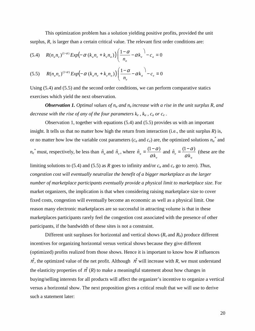
This optimization problem has a solution yielding positive profits, provided the unit
surplus, R, is larger than a certain critical value. The relevant first order conditions are:
(5.4) ( ) 01)()( )1( =−�
���
�−−+−−
aea
aeeaea ckn
nknkExpnnR αααα
(5.5) ( ) 01)()( )1( =−�
���
�−−+−−
eae
aeeaea ckn
nknkExpnnR αααα
Using (5.4) and (5.5) and the second order conditions, we can perform comparative statics
exercises which yield the next observation.
Observation 1. Optimal values of na and ne increase with a rise in the unit surplus R, and
decrease with the rise of any of the four parameters ke , ka , ca or ce .
Observation 1, together with equations (5.4) and (5.5) provides us with an important
insight. It tells us that no matter how high the return from interaction (i.e., the unit surplus R) is,
or no matter how low the variable cost parameters (ca and ce) are, the optimized solutions na* and
ne* must, respectively, be less than an̂ and en̂ , where
ea k
nαα )1(ˆ −= and
ae k
nαα )1(ˆ −= (these are the
limiting solutions to (5.4) and (5.5) as R goes to infinity and/or ca and ce go to zero). Thus,
congestion cost will eventually neutralize the benefit of a bigger marketplace as the larger
number of marketplace participants eventually provide a physical limit to marketplace size. For
market organizers, the implication is that when considering raising marketplace size to cover
fixed costs, congestion will eventually become an economic as well as a physical limit. One
reason many electronic marketplaces are so successful in attracting volume is that in these
marketplaces participants rarely feel the congestion cost associated with the presence of other
participants, if the bandwidth of these sites is not a constraint.
Different unit surpluses for horizontal and vertical shows (Rv and Rh) produce different
incentives for organizing horizontal versus vertical shows because they give different
(optimized) profits realized from those shows. Hence it is important to know how R influences
π*, the optimized value of the net profit. Although π* will increase with R, we must understand
the elasticity properties of π* (R) to make a meaningful statement about how changes in
buying/selling interests for all products will affect the organizer’s incentive to organize a vertical
versus a horizontal show. The next proposition gives a critical result that we will use to derive
such a statement later:

21
Proposition 5.
a) π* is zero up to a critical value of R, after which it is strictly increasing in R.
b) π* is convex, asymptoting to a straight line with a positive slope and negative intercept.
c) The elasticity of the π* curve is decreasing in R.
Thus, the π* curve as a function of R, for fixed α, ka, ke, ca and ce, looks like as
represented in Exhibit 2, with the dashed line its asymptote. The intercept of the asymptote is
given by (the negative of) the variable cost at the critical values an̂ and en̂ , and its slope is given
by ( an̂ en̂ )(1-α) Exp (- α (ke an̂ + ka en̂ )).
Let *hπ and *
vπ represent the optimal profits from a horizontal and a vertical show
respectively (net of variable but gross of fixed costs). A corollary to Proposition 5 that gives us a
useful result is:
Corollary 1. Suppose α, ka, ke, ca and ce are fixed. If in addition, vR is fixed (and hence
*vπ fixed), ** / vh ππ is an increasing function of hR .
Hence, given fixed vertical show unit surplus Rv , we only need to investigate how market factors
affect hR in order to understand incentives to organize horizontal versus vertical shows.
B. Determination of the Number and Mix of Vertical and Horizontal Shows: So far we
know what determines the relative profits of a horizontal and a vertical show. One can produce
several arguments why the ratio of these (optimized) profits should directly influence the
proportion of horizontal shows in an industry. We present one such argument here, while noting
that there are other plausible setups leading to the same conclusion3.
Let Nv and Nh represent the number of vertical and horizontal shows in an industry. In our
framework, in equilibrium these numbers depend on the fixed costs as well as the market
structure of the organizing industry. Fixed costs arise from rental of show space, pre-show
promotion and advertising, commitments to entertainment events, staff commitments and the
3 For instance, assume a fixed number of organizers in an industry each of whom can organize just one show andeach of whom has a logarithmic utility function U(.) for money. Also assume that the actual utilities that aparticular organizer will obtain from a show (horizontal or vertical) will be U(.) of the corresponding show’s profit( *
hπ or *vπ ) plus a random disturbance term (e.g. Actual Utility (Horizontal) = ln *
hπ + ξ ). If the randomdisturbance term (ξ ) follows IID extreme value distribution, then following standard random utility based choicemodel arguments (see e.g., McFadden (1974)) one can show that the proportion of horizontal shows in the industrywill be given by the ratio *
hπ / ( *hπ + *
vπ ). While this setup gives an explanation for the proportions of show types,we prefer our setup as it provides insight into the number of shows of each type as well.

22
like. A simple way to characterize these fixed costs is to assume that a vertical show requires one
unit of a ‘vertical fixed factor’ and a horizontal show requires one unit of a ‘horizontal fixed
factor,’ where a unit factor comprises a unit vector of the fixed cost components. Organizers
purchase these factors and their prices are influenced by the demands of both factors. Letting Pv
and Ph denote the prices of these fixed factors, we postulate simple, linear price-quantity
relationships:
(5.6) hvv NmNmP 21 +=
(5.7) vhh NmNmP 43 +=
We also assume that effect of own demand on price exceeds the effect of cross demand.
That is m1 and m3 are assumed to be larger than m2 and m4; more precisely, Min(m1 , m3) >
Max(m2 , m4). Our assumptions imply that the factors for the two types of shows are not identical
(in which case m1 would equal m2 and m3 would equal m4), but there is a certain amount of
substitutability between them. For example, vertical and horizontal shows might compete for the
same convention center, but might use different media to reach prospective participants and
attempt to hire different types of entertainers.
We now analyze how Nv and Nh arise under different market structures. Assume first that
the organizing industry is a monopoly. Then the sole show organizer solves an optimizing
problem of the following sort:
(5.8) Maximize *vπ Nv + *
hπ Nh – ( hv NmNm 21 + ) Nv – )( 43 vh NmNm + Nh.
The first order conditions for this optimization problem enable us to solve for the optimal
numbers of each type of show. The ratio of the optimized profits plays a critical role in
determining the proportion of horizontal shows (ph), as the following key proposition shows:
Proposition 6. Under the condition of a monopolistic organization industry,
a) ph is 0 (i.e. Nh is 0) if ** / vh ππ is less than or equal to (m2 + m4) / 2m1 .
b) ph increases with a rise in ** / vh ππ as long as the latter is within
( (m2 + m4) / 2m1 , 2m3 / (m2 + m4) ).
c) ph is 1 (i.e. Nv is 0) if ** / vh ππ equals or exceeds 2m3 / (m2 + m4).
Consider next a competitive market structure. Under perfect competition, entry of new shows
will occur as long as the average revenue from a show, π* , stays above its average cost, which in
our case is the price of the corresponding fixed factor. This ‘zero profit condition’ allows us to
23
determine the dependence of ph on the ratio of the optimized profits from the two types of the
shows which we describe in the next proposition.
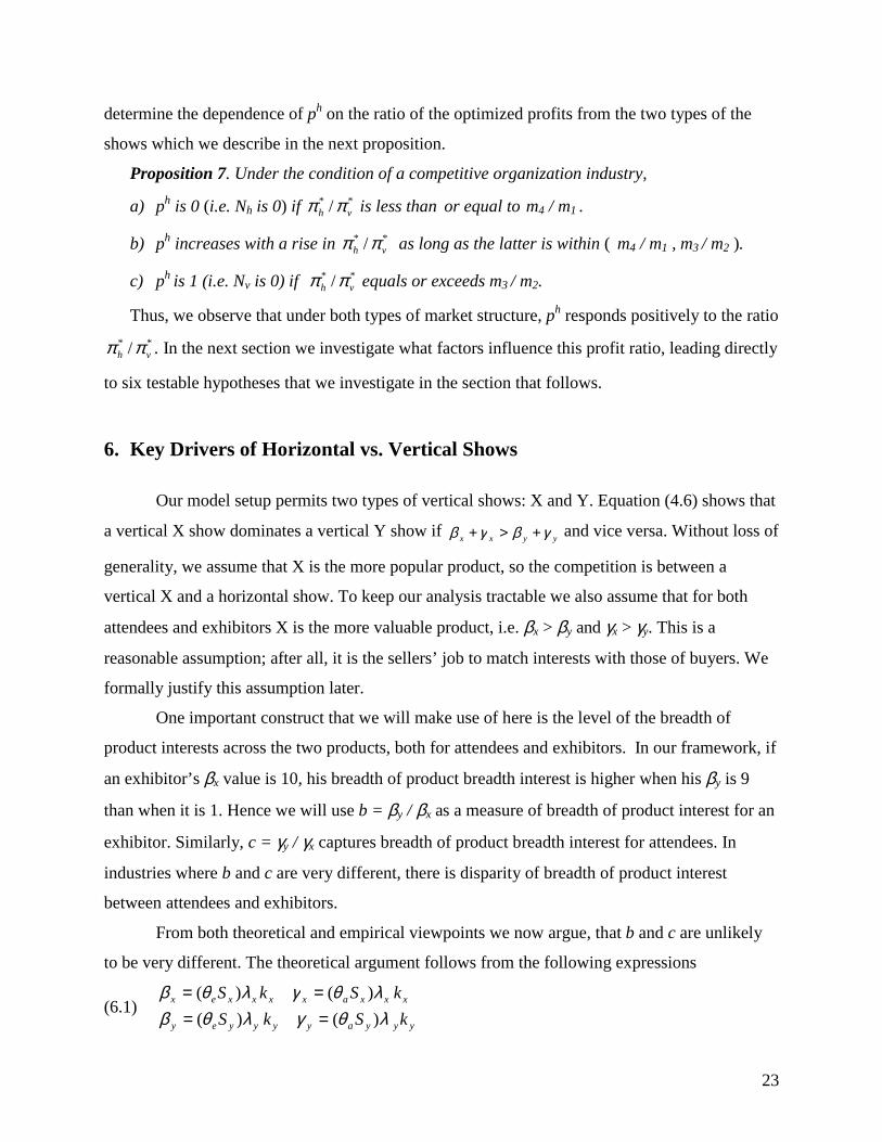
Proposition 7. Under the condition of a competitive organization industry,
a) ph is 0 (i.e. Nh is 0) if ** / vh ππ is less than or equal to m4 / m1 .
b) ph increases with a rise in ** / vh ππ as long as the latter is within ( m4 / m1 , m3 / m2 ).
c) ph is 1 (i.e. Nv is 0) if ** / vh ππ equals or exceeds m3 / m2.
Thus, we observe that under both types of market structure, ph responds positively to the ratio** / vh ππ . In the next section we investigate what factors influence this profit ratio, leading directly
to six testable hypotheses that we investigate in the section that follows.
6. Key Drivers of Horizontal vs. Vertical Shows
Our model setup permits two types of vertical shows: X and Y. Equation (4.6) shows that
a vertical X show dominates a vertical Y show if yyxx γβγβ +>+ and vice versa. Without loss of
generality, we assume that X is the more popular product, so the competition is between a
vertical X and a horizontal show. To keep our analysis tractable we also assume that for both
attendees and exhibitors X is the more valuable product, i.e. βx > βy and γx > γy. This is a
reasonable assumption; after all, it is the sellers’ job to match interests with those of buyers. We
formally justify this assumption later.
One important construct that we will make use of here is the level of the breadth of
product interests across the two products, both for attendees and exhibitors. In our framework, if
an exhibitor’s βx value is 10, his breadth of product breadth interest is higher when his βy is 9
than when it is 1. Hence we will use b = βy / βx as a measure of breadth of product interest for an
exhibitor. Similarly, c = γy / γx captures breadth of product breadth interest for attendees. In
industries where b and c are very different, there is disparity of breadth of product interest
between attendees and exhibitors.
From both theoretical and empirical viewpoints we now argue, that b and c are unlikely
to be very different. The theoretical argument follows from the following expressions
(6.1)yyyayyyyey
xxxaxxxxex
kSkSkSkS
λθγλθβλθγλθβ)()(
)()(====

24
where Sx, Sy are the total surplus (attendee’s valuation minus exhibitor’s cost) for a unit
transaction in X and Y respectively; θe and θa are the shares of this surplus for the exhibitor and
the attendee respectively (θe + θa =1), λx and λy are the transaction intensity factors for the
exhibitor-attendee pair for the two products and kx, ky are technology parameters for the
production function (see equation 3.1). Then simple division confirms that both b and c are given
by Sykyλx / Sxkxλy and hence are equal.
For an empirical counterpart of this closeness argument, consider Exhibit 4, where we
describe data compiled on breadth of exhibitor and attendee interests across industries, and the
hypothesis that this difference (averaging 0.238 on a 1-7 Likert scale) is not different from zero
cannot be rejected. From (6.1) we also see that if θe is close to θa then βx is likely to be close to γx
as well (and βy should be close to γy). Indeed, if the bargaining abilities of the two parties
(captured by their shares of the surplus) are not very different, then these shares of surplus are
likely to be close. Hence, if the attendees prefer X to Y so will the exhibitors and vice versa.
With the aid of Propositions 5, 6 and 7 we now investigate the factors that influence ph,
the proportion of horizontal shows in an industry. The parameters of our model will affect this
ratio in a number of subtle ways, but all will work through their influence on the movement of Rh
relative to Rv and/or the movement of the π* curve itself (and hence the movement of ** / vh ππ ).
We will present theoretical propositions and related proofs, and will also provide numerical
simulations showing that our results hold even for many plausible values of the model
parameters outside the conditions identified in the propositions.
To provide background for our next four propositions, consider Exhibit 3 which provides
Rh / Rv ratios for various values of our model parameters. Holding γx at a (normalized) value of 1,
we present the numerical values of Rh / Rv for various b’s and c’s ranging from 0.2 to 1 (in steps
of .2). The other parameter values we chose were all possible combinations of βx = 1, 3, 5 and α
= .05, .25, .45. It is unlikely that the benefit that attendees (exhibitors) get out of a transaction is
likely to be more than a small multiple of the benefit the attendees (exhibitors) get; so we limited
our simulations to βx less than 5.
Although, it is difficult to draw firm conclusions from Exhibit 3 data alone, it seems that
Rh is typically at least as large as Rv. The only cases where this condition is violated involve very
large values of c compared to b and very high values of α, conditions which we have previously

25
argued, are unlikely. Further, if either b is close to c or if βx is close to γx, Rh will always be
larger than Rv. The following observation covers both cases.
Observation 2. Rh strictly exceeds Rv in an open neighborhood of parameters satisfying
(6.2) 0))(( ≥−− cbxx γβ .
Note that this is only a sufficient condition. Also note that if one assumes that βx
(slightly) exceeds γx (i.e. exhibitors see more benefit than attendees per meeting for the X good),
this condition is likely to be satisfied, as our data show that exhibitors have (slightly) higher
breadth of product interest than do attendees.
We now develop propositions on drivers of the ratio of horizontal to vertical shows. For
the first two propositions, the change in the relevant parameter will not affect Rv (i.e. xx γβ + ), so
by Corollary 1 we only need to examine the effect of the relevant parameter on Rh. For the third,
both Rv and Rh change. Finally for the fourth, Rv remains fixed while Rh changes, but in addition,
the π* curve itself shifts.
A. The Impact of Breadth of Product Interest of Exhibitors and Attendees. Horizontal
shows address a broader set of products than do vertical shows, and one might expect to see that
as the breadth of interest in products increases (as reflected in increases in the b and c
parameters), we would see more of such shows. Specifically, we investigate what happens to Rh,
if keeping βx, γx and α fixed, we change b and c. Exhibit 3 suggests that a rise in b or c generally
raises Rh (Rv remains fixed), although some slight exceptions can be found. For instance when α
= .45, βx = 3, γx = 1, and c = 1, raising b from .2 to .4 actually lowers Rh. These occurrences seem
surprising as it means that if we hold the attendees’ product valuations fixed, and do not change
the valuation of the preferred product for an exhibitor, an increase in the exhibitors’ less
preferred product’s valuation can hurt the revenues and hence profits for a horizontal show. This
result can be understood by noting that such a change may end up producing new effort
allocation schemes by participants in accordance to the equilibrium results of Section 4. The
change in effort allocations may, in turn, decrease total (equilibrium) surplus and hence, total
revenues. However this situation should be the exception rather than the rule as the table and the
following proposition suggest.
Proposition 8. In an open neighborhood of the set of parameters that satisfy condition
(6.2), Rh (and, hence ** / vh ππ because vR is fixed) is strictly increasing in b or c. Therefore,
breadth of product interest has a positive impact on the proportion of horizontal shows, ph.

26
B. The Impact of Difference of Breadth of Product Interest Between Exhibitors and
Attendees. Next we ask how the difference in the breadth of product interest between attendees
and exhibitors affects the proportion of horizontal shows. If these interests are too disparate, we
might expect a “coordination problem” that is harmful for surplus generation. More formally we
ask whether, keeping the sum of b and c fixed, it helps the horizontal show proportion if b and c
are closer to each other. The answer is clear when βx is close to γx or when b is close to c:
Proposition 9. Suppose βx and γx are sufficiently close. Then
a) If b > c, the following holds:
(6.3) 0// <∂∂−∂∂ cRbR hh .
Vice versa, if c > b, the inequality above is reversed.
b) If b = c, irrespective of βx and γx, the following holds:
(6.4) 0// =∂∂−∂∂ cRbR hh .
c) If b > c, and b is close to c, the following holds:
(6.5) 0// <∂∂−∂∂ cRbR hh .
Vice versa, if c > b, and they are close, the inequality above is reversed.
Thus, when βx is close to γx or when b is close to c, an increase in | b-c|, keeping the sum b+ c
fixed, decreases Rh (hence decreases ** / vh ππ because vR is fixed). Therefore, the absolute
difference in range of product breadth between exhibitors and attendees has a negative impact
on the proportion of horizontal shows, ph.
C. The Impact of Selling/Buying Intensity of Exhibitors and Attendees. Next we ask
what happens if all four of the product valuation parameters (βx, βy, γx, γy) decrease
proportionally, (signaling, in effect, a rise in non-selling or information gathering propensity or
λ)? In the proof of the next proposition we show that the answer relates to the elasticity of the
π*(R) curve: higher R values result in lower elasticity. Hence, a rise in both non-selling and non-
buying interests lowers *vπ relatively more than *
hπ , thus benefiting the proportion of horizontal
shows.
Proposition 10. Suppose Rh is larger than Rv. Then, a percentage decrease in all the beta
and gamma values (βx, βy, γx, γy) increases ** / vh ππ . Therefore, increase in non-selling interest for
exhibitors and non-buying interest for attendees has a positive effect on the proportion of
horizontal shows, ph.

27
Proposition 10 helps explain why in industries with relatively more horizontal than
vertical shows, we are also likely to see participants who have more non-selling and non-buying
interests and thus, a smaller transaction intensity factor λ. In a related manner, one can see why
on average, vertical shows will be more closely associated with lead generation, given that the
latter measure is more likely to track immediate rather than distant (product) transactions.
D. The Impact of Technological Innovativeness in an Industry. Shows in fast moving,
innovative industries have more technical issues to communicate, and typically display many
state-of-the-art products which are completely new and unfamiliar to the majority of attendees.
When one starts from ground zero there is a lot to learn, which implies that the rate of
information transmission for the first few units of joint effort will be high relative to the same
rate for the last few units of available effort. Thus α (a measure of diminishing marginal returns
and hence, gains to diversification), will be lower for such industries.
How will α affect ph? There are two different diversification effects to consider here.
First, there is the ‘product diversification effect’. Sharper diminishing marginal returns are likely
to provide more benefit when there are more products to allocate efforts to. Analytically, this
relates to how α will change Rh (without affecting Rv ). We see from Exhibit 3 that generally, a
lower α raises Rh , which is conducive to horizontal shows.
Lemma 1. Fixing the betas and gammas, a lowering of α raises Rh (hence raises** / vh ππ because vR is fixed) in an open neighborhood of parameter values satisfying (6.2).
The second effect to consider is the ‘participant diversification effect’. Intuitively, with
more participants among whom to spread efforts, the gains to diversification due to changes in
marginal returns will have a greater impact. Analytically, this effect refers to the movement of
the π* curve itself as α changes. Under certain simplifying and plausible approximations one can
show that this effect is also conducive to horizontal shows.
Lemma 2. Suppose R1 and R2 are large fixed values such that the asymptote to the π*
curve approximates the curve itself closely at these values. Also, suppose R1 > R2 and ka and ke
are small (it suffices to assume ka ke < e-2). Then, π*(R1) / π*(R2) increases as α decreases.
Combining lemmas 1 and 2, we have:
Proposition 11. Under the assumptions made in Lemmas 1 and 2, a lowering of α raises** / vh ππ . Therefore, the technological innovativeness of an industry has a positive impact on the
proportion of horizontal shows, ph.

28
We reiterate that we derive propositions 8-11 (like Observation 2) using certain sufficient
conditions. We have argued that these sufficient conditions are likely to hold, the conclusions are
nevertheless true for a much larger set of parameters (which we have not been able to
characterize in closed, interpretable form). We now turn our attention to an empirical assessment
of these propositions.
7. Empirical Analysis
A. Data Collection and Hypothesis Generation. To link our theoretical results to the
Exhibit 1 patterns that motivated our key questions, we needed data on industry characteristics
that related to our key model constructs, especially those highlighted in Propositions 9-12:
breadth of product interest, selling/buying intensities of participants’, and technological
innovativeness. The Exhibit 1 database, representing 1152 trade shows in 21 industries provided
our sample frame. In order to capture the other data, we needed evaluations that would be
comparable across industries. For selling/buying intensities and breadth of interest, we needed
experts who had trade show specific, cross industry knowledge. We selected two experts who
were executives at a major trade show research firm and asked them individually to complete a
questionnaire with the following 4 questions
On a 1-7 Likert scale (1=lowest, 7=highest):
1) For an average attendee in each of the following industries, please rate his/her buying
intensity at a typical show;
2) For an average attendee in each of the following industries, please rate his/her breadth
of product interests at a typical show
3) For an average exhibitor in each of the following industry, please rate his/her selling
intensity at a typical show
4) For an average exhibitor in each of the following industry, please rate his/her degree of
interest in contacting attendees with different product interests
When the two experts’ answers differed significantly, we recycled their answers to them
and asked them to resolve those differences. After two rounds their answers essentially
converged and we averaged any (small) remaining differences.

29
To assess technological innovativeness, trade show knowledge was not an issue in
selecting experts. We contacted 17 well-known experts in new product development and
technological innovation and asked each to rate the 21 industries (again on a Likert 1-7 scale) on
degree of innovativeness, defined as “the relative amount of new product development and new
technical information that occurs per year within the industry”. Here, the experts generally
agreed after the second round: the median was quite close to the mean and all our results were
robust to the use of either value.
Exhibit 4 summarizes the mean values of the experts’ rankings of the different variables.
A review of that Exhibit shows that the numbers in columns 4 vs. 5 tend to stay close together.
Indeed, the mean difference between (4) and (5) is 0.28 with standard deviation of 1.01. We
cannot reject the hypothesis that within-industry attendee/exhibitor differences in breadth of
product interests are the same at the p = 0.001 level for either pair of variables. Hence, this
preliminary look at the data confirms that the sufficient conditions we used to prove
Observations 2,3 and Propositions 8-11 do hold (b is empirically very close to c). Hence, our
data appear appropriate to justify their use to test the following hypotheses generated from the
propositions in the last section:
A larger proportion of horizontal trade shows in an industry, ph will be associated with:
H1. A larger breadth of product interests for attendees (ATPROD); (column 4, Exhibit 4).
Source: Proposition 8.
H2. A larger breadth of product interests for exhibitors (EXPROD); (column 5, Exhibit 4).
Source: Proposition 8.
H3. A smaller difference in breadth of product interests (DIFFPROD); (Absolute difference
between columns 4 and 5, Exhibit 4). Source: Proposition 9.
H4. A smaller buying intensity of the attendees (ATBUY); (column 2, Exhibit 4) Source:
Proposition 10.
H5. A smaller selling intensity of the exhibitors (EXBUY); (column 3, Exhibit 4) Source:
Proposition 10.
H6. A higher level of industry technological innovativeness (TECH); (column 1, Exhibit 4).
Source: Proposition 11.
B. Analysis/Results. We ran several regression models to test these hypotheses. In all
cases, we weighted the observations by the total number of shows in the industry. The models

30
run were: a) standard OLS, b) an OLS model with the dependent variable being a logistic
transformation of doubly truncated p; i.e. Max {a, Min {p, b}} where a and b are the lower and
upper truncation limits (we tried a=.01, b= .99; a=.05, b=.95 and a=.1, b=.9 as different sets of
truncation limits) c) probit and d) logit. While all models generally gave consistent results, the
standard logit model dominated the others in terms of fit. Henceforth, we use the term ‘better fit’
in the sense of lower AIC; the Akaike Information criterion (Akaike (1973), (1974)), where that
AIC for a model is –2*Log Likelihood + 2*(number of parameters in the model).
Exhibit 5 presents our results. The first four columns in that Exhibit present the result of
running the four models mentioned above (the truncation limits used for the version of the
second model reported here are .01 and .99). As can be seen, the logit model gives the best fit.
All models strongly reject the hypothesis that the explanatory variables are jointly insignificant;
and all variables are individually highly significant with the hypothesized signs except TECH in
the OLS model. Apart from this one exception all variables are significant at 5% or beyond and
most are significant at the1% level and beyond. We also tested if disaggregating attendee and
exhibitor characteristics provides a more powerful explanation of the data than in the aggregated
case, a concern as these pairs of characteristics, do not differ by much. To check on the effect of
disaggregation, we ran the logit model dropping ATBUY, EXBUY, ATPROD and EXPROD,
but introducing TOTBUY (ATBUY+EXBUY) and TOTPROD (ATPROD+EXPROD), reported
in the fifth column of Exhibit 5. The results favor the disaggregated version. Finally, we ran one
set of regressions using SDIFPROD instead of DIFFPROD (a scaled version of DIFFPROD;
defined as DIFFPROD divided by TOTPROD), and found the fit to be slightly better with
DIFFPROD.
To summarize the results of this section, our empirical analysis confirms all 6
hypotheses, H1 through H6, at significance levels 5% or better.
C. Predictive Validation and Discussion. In order to test the predictive validity of our
model, we used a jackknife approach: for each industry we used the data from the other twenty
industries as the calibration sample and predicted the proportion of horizontal shows for this hold
out industry. The residual is the difference between the empirical proportion of that industry’s
shows that are horizontal and the predicted proportion, based on the coefficients of the logistic
analysis from the calibration sample. Exhibit 6 gives the results (along with full sample fitted
values and residuals).

31
From Exhibit 6 we note that, from a predictive validity perspective, our model does quite
well. More than half our sample comes from the first two categories; yet our prediction error for
Computers is only 8.4% while it is 0.4% for Communications. These compare to an average
Mean Absolute Deviation (MAD) of 6.6 % for the sample as a whole (on an unweighted basis).
Indeed, one of the industries—Packaging—appears to be an outlier. If we drop Packaging, we
get a MAD of 2.5% for fitted values and 4.8% for predicted values.
One can look at the jackknife results from a different perspective. If our model
characterizes the behavior of efficient industries well, then it appears that the Packaging and the
Building and Construction industries may be overserved by horizontal shows (large positive
residuals) while the Chemicals and Manufacturing industries appear to be underserved (large
negative residuals). The two industries with the largest numbers of shows, namely
Computers/Computer Applications and Communications appear to have about the right mix
according to our model.
Recall that we have used expert judgment data to construct our predictor variables here.
With such data it is always possible that if the experts believe in the theory (even if it is false)
they will provide confirming evidence. Although we cannot dismiss this possibility out of hand,
our hypotheses and models are sufficiently subtle to suggest that this is highly unlikely. For
example, if one tries to infer just by looking at our data table in what direction an independent
variable influences the dependent variable, one might be misled. Consider TECH. Since the
samples are weighted by the number of shows in the industries, one might suppose that the two
top industries by this category, namely Computers & Computer Applications and
Communications will influence the results heavily since together they account for 61% of the
shows in the sample. They also have the two highest scores in terms of TECH (6.58 and 6.32
respectively). Now, given that the proportions of horizontal shows in these two industries are
small (17% and 1% respectively), one might conclude that TECH influences the dependent
variable negatively. Yet, our analysis shows that after controlling for other variables, we find
TECH has a positive influence on ph. This instance suggests that our model has subtle
contingencies that experts would have found difficult to (mentally) control for in giving their
responses.
However, these empirical results are preliminary and depend on the judgment of a limited
number of expert evaluators. Clearly more work is needed to evaluate these results more
soundly, but this preliminary investigation at least supports our theoretical results in a rewarding
32
manner. The results also suggest how such findings can be both of theoretical and managerial
value.
8. Conclusions
We have argued that given certain key characteristics of potential participants, each
marketplace has an optimal size and structure. While motivated to a degree from observations
from the trade show marketplace and corroborated to a rewarding extent from an empirical
analysis in that arena, we have used little institutional structure specific to that arena in
developing our main results. Any market characterized by time-consuming search processes for
information leading to ‘matches’ between brands and needs can be subject to this type of
analysis. We have been unable to locate other studies involving the three sets of market
participants we study here and the costs and benefits of their interaction as the factors that lead to
marketplace structure and formation. Hence our results are best treated as exploratory. Below,
we discuss the restrictiveness of some of our modeling choices and how these invite further
research, while pointing out why most of our results are likely to hold under more general
frameworks.
Our model depends on specific functional forms of production functions and congestion
costs. While the functions we chose were quite specific, our main results derive from the
(ultimately) decreasing returns to additional interaction balanced against an increasingly costly
congestion effect. Admittedly, the fact that for Cobb-Douglas functions marginal returns to effort
is infinity at zero effort levels is what gives us the ‘equal-division’ results in Section 4; however,
as long as the marginal returns to effort at zero high enough (and the cost parameters are non-
negligible) we should obtain similar results. Also note that the congestion cost function for a
participant could be generalized to include as its arguments both total number of participants as
well as the number of participants actually visited. These features will complicate the analysis
substantially, but in all likelihood, will not alter the general conclusion that marketplaces will
have limited sizes determined by product valuation parameters, extent of diminishing marginal
returns (positive impact), and cost coefficients (negative impact).
We looked at two products in a marketplace and framed a horizontal show as one that had
both of those products. In a two-product world, breadth of product interest is easy to define as
the ratio of the two product valuation parameters. In a multiple product world there is no such

33
obvious summary statistic; and hence we are unsure about the formats Propositions 8 and 9 are
likely to assume in such a case. But the fundamental insight here is that if the two sides of a
market are interested in different things, it may not pay the organizer to allow them to pursue
their own interests – which is why a vertical show, by forcing all participants to concentrate on a
narrow range of products may avoid this harmful conflict of interest.
An assumption that is critical to our model is that of both attendee and exhibitor
homogeneity in terms of product valuations, although we have incorporated heterogeneity of
brand preferences. As the segmentation literature shows (Wedel and Kamakura, 1998), one can
provide an explanation for almost any market structure by appealing to heterogeneity arguments.
While that is certainly true, the insight that our results provide is that these different market
structures can be derived even under the conditions of homogeneity. While adding heterogeneity
to the model would clearly enrich the structure, we have not been able to develop results with
heterogeneous populations that provided any clear insights.
Our results were also driven by the specific cost functions that we specified. The reader
may question why variable costs are linear in their arguments while fixed costs are not. We
conjecture that if marginal variable costs were increasing, the propositions relating to limiting
size and the shape of the π* function will remain unchanged. Also, future empirical work should
consider industry specific factors that affect these costs, and hence the mix between horizontal
and vertical shows.
Finally, while we are encouraged by our empirical results, we have noted that the data
that support these results are based on judgmental data from experts. It would be desirable to
validate these findings using data gathered from actual as well potential show participants. Such
data should also be able to pick up the effects of heterogeneity in the participant pool on
variables of interest.
As with any theoretical model, at the cost of a certain amount of abstraction we have
been able to gain considerable insight. It may well be that other richer model structures can
extend these findings or lead to others in this or in related marketplaces. Indeed, the booming
electronic analogy of our development here is the portals marketplace, with Chemdex.com
(1999) and Plastics.net examples of vertical portals, Vertical.net an example of a portal organizer
that helps set up vertical portals, and Industry.net an example of a horizontal portal.. We hope
that an extension of our model framework will permit a better understanding of such
developments, extending our findings from the marketplace to marketspace.

34
References
Akaike, H. (1973), “ Information Theory and an Extension of the Maximum LikelihoodPrinciple,” in B. N. Petrov and F. Csa’ki eds. , 2nd International Symposium on InformationTheory, Akade’miai KiadÓ, Budapest, 267-281.
Akaike, H. (1974), “A New Look at the Statistical Model Identification”, IEEE Transactions onAutomatic Control, AC-19, 716-723.
Axelson, Barbara (1999), “Trade shows gain larger share of marketing budgets; computers helpMake manufacturing top category, Advertising Age's Business Marketing; 84 (May) 14-15.
Balderston, F. E. (1958), “Communication Networks in Intermediate Markets”, ManagementScience, Vol. 4 (January), 154-171.
Baligh, Helmy H. and Leon E. Richartz (1967): Vertical Market Structures, Allyn and Bacon,Inc. Boston.
Beath, John and Yannis Katsoulacos (1991): The Economic Theory of Product Differentiation,Cambridge University Press, Cambridge, UK.
Chemdex.com (1999), Harvard Business School Case 9-89-076, revised June 1999.
Dasgupta, Ani, Gary L. Lilien and Jianan Wu (2000), “ A Theory of Size and Product Diversityof Marketplaces with Application to the Trade Show arena”, ISBM Report, 2-2000, available athttp://www.smeal.psu.edu/isbm
Dekimpe G. Marnik, Pierre Francois, Srinath Gopalakrishna, Gary Lilien and Christophe Vanden Bulte (1997), “Generalizing About Trade Show Effectiveness: A Cross-NationalComparison”, Journal of Marketing, 61(October), 55-64.
Dixit, Avinash K. and Joseph E. Stiglitz (1977), “Monopolistic Competition and OptimumProduct Diversity”, American Economic Review, 67, 297-308.
Fudenberg, Drew and Jean Tirole (1993): Game Theory, MIT Press, Cambridge.
Gopalakrishna, Srinath and Jerome D. Williams (1992), “Planning and Performance Assessmentof Industrial Trade Shows: An Exploratory Study”, International Journal of Research inMarketing, 9, 207-224
Gopalakrishna, Srinath and Gary L. Lilien (1994), “A Dynamic model of Business Trade ShowEffectiveness”, ISBM Report, 3-1994.
Hansen, Kare (1996), “The Dual Motives of Participants at Internaltional Trade Shows: AnEmpirical Investigation of Exhibitors and Visitors with Selling Motives,” InternationalMarketing Review, 13(2), 39-53.

35
Hansen, Kare (1999), “Trade Show Performance: A Conceptual Framework and Its Implicationsfor Future Research,” Academy of Marketing Science Review, [Online] 99 (08) Available:http://www.amsreview.org/amsrev/theory/hansen08-99.html.
Hotelling, Harold H. (1929), “Stability in Competition”, Economic Journal, 39, 41-57.
Kerin, Roger A. and William L. Cron (1987), “Assessing Trade Show Functions andPerformance: An Exploratory Study'', Journal of Marketing, 51, 87-94
Kotler, Philip (1999), Marketing Management, 10th edition, Prentice-Hall Inc.
Lilien, Gary L. (1983), “A Descriptive Model of the Trade Show Budgeting Decision Process'',Industrial Marketing Management, 12, 25-29.
McFadden, Daniel (1974), “Conditional Logit Analysis of Qualitative Choice Behavior”, inFrontiers in Econometrics by Paul Zarembka (ed), Academic Press, New York and London.
Reitman, David, “ Endogenous Quality Differentiation in Congested Markets”, The Journal ofIndustrial Economics, XXXIX, 621-647.
Selten, R. (1975), “Re-examination of the Perfectness Concept for Equilibrium Points inExtensive Games”, International Journal of Game Theory, 4, 25-55.
Van Damme, E. (1992): Stability and Perfection of Nash Equilibria (2nd. edition), Springer-Verlag, Berlin.
Wedel, Michel and Wagner Kamakura, (1999) Market Segmentation: Conceptual andMethodological Foundations, 2nd Edition (Kluwer: Boston)
Williams, Jerome D., Srinath Gopalakrishna and J.M. Cox (1993), “Trade Show Guidelines forSmaller Firms”, Industrial Marketing Management, 22, 265-275.

36
LIST OF NOTATION USED IN THE TEXT(in order of appearance)
Notation DefinitionX, Y Different product categoriesU Benefit accrued to a party due to effort investment (by both parties)k A constant in the production functionr (Common) rate of interest used by attendees and exhibitorsλ Transaction intensity factorv (Net) value to a party per unit transaction in the exhibitor’s productp Effort expended by exhibitor in the interactionq Effort expended by attendee in the interactionα A parameter in the production function that captures the extent of diminishing marginal returnsβ Product valuation parameter for exhibitor (product of v, ρ, k)γ Product valuation parameter for attendee (product of v, ρ, k)na Number of attendees in a showne Number of exhibitors in a showφa A function appearing in attendees’ congestion cost functionφe A function appearing in exhibitors’ congestion cost functionTa Total time available to attendees (net of congestion cost) for investment in information gatheringTe Total time available to exhibitors (net of congestion cost) for investment in information disseminationka Parameter determining how ne affects TaTeke Parameter determining how ne affects TaTepij Effort expended by exhibitor i toward attendee j (in a vertical show)qji Effort expended by attendee j toward exhibitor i (in a vertical show)βx, βy Product valuation parameter for exhibitors specific to products X and Y respectivelyγx, γy Product valuation parameters for attendees specific to products X and Y respectivelypijx , pijy Effort expended by exhibitor i toward attendee j in disseminating information about products X and Y respectively
(in a horizontal show)

37
qjix , qjiy Effort expended by exhibitor i toward attendee j in disseminating information about products X and Y respectively(in a horizontal show)
ca Variable cost for each extra attendeece Variable cost for each extra exhibitorπ Organizer’s profit function net of variable but gross of fixed costs (depends on na, ne, R, α, ka, ke , ca , ce)R Surplus generated by an attendee-exhibitor pair if they each had one unit of time to devote to the otherRv R for a vertical showRh R for a horizontal showna
* Optimal number of exhibitors in a showne
* Optimal number of attendees in a showan̂ An endogenously determined limit on the optimal number of attendees
en̂ An endogenously determined limit on the optimal number of exhibitorsπ* A function that takes R as an argument and generates optimized profits for that R by choosing the best na and ne
(parametrized on α, ka, ke, ca and ce )*hπ Optimized profits (gross of fixed but net of variable costs) for a horizontal show ( π* (Rh) )*vπ Optimized profits (gross of fixed but net of variable costs) for a vertical show ( π*(Rv) )
Nv Number of vertical shows in an industryNh Number of horizontal shows in an industryPv Price of ‘vertical fixed cost factor’Ph Price of ‘horizontal fixed cost factor’m1 , m2 Demand function parameters for the ‘vertical fixed factor’m3 , m4 Demand function parameters for the ‘horizontal fixed factor’ph Proportion of horizontal shows in an industryb Product breadth interest parameter for exhibitorsc Product breadth interest for attendeesSx, Sy Surplus generated in 1 unit of product exchange for the X and Y goods respectivelyθe,θa Exhibitor and attendee shares of this surplus

38
Group Industry Number ofVerticalShows
Number ofHorizontal
Shows
TotalNumberof Shows
Proportionof Horizontal
ShowsOver 100 Shows Computers & Computer Applications 379 78 457 17%
Communications 319 3 322 1%
50-100 Shows Engineering 3 93 96 97%Medical & Health Care 90 4 94 4%Housing 80 0 80 0%Food Processing & Distribution 3 61 64 95%Electrical & Electronics 52 7 59 12%
15-50 Shows Paint 49 0 49 0%Nursing 48 0 48 0%Automotive & Trucking 3 44 47 94%Chemical 20 23 43 53%Plastics 0 33 33 100%Radio, TV & Cable 32 1 33 3%Energy 0 30 30 100%Building & Construction 15 10 25 40%Restaurants & Food Service 0 24 24 100%Manufacturing 6 15 21 71%Photographic 21 0 21 0%Welding 17 0 17 0%Packaging 0 15 15 100%Education 15 0 15 0%
Total 1152 441 1593 28%
Exhibit 1. A Selection of Industries and the Associated Number and Distribution of Trade Show Types (1985-1991),Showing the Wide Diversity in the Proportion of Horizontal Shows
Source: Exhibit Surveys Inc. Note: industries with fewer than 15 trade shows have been omitted from this chart due the instability of the proportions when thetotal number of shows in the industry is that low.

39
Exhibit 2: How Show Organizer’s Profits Increase with R, the Unit Surplus of an Attendee-Exhibitor Pair
R
Profits

40
αααα=.05 αααα=.25 αααα=.45b\c 0.200 0.400 0.600 0.800 1.000 0.200 0.400 0.600 0.800 1.000 0.200 0.400 0.600 0.800 1.000
ββββX=10.200 1.149 1.232 1.316 1.401 1.487 1.019 1.042 1.068 1.098 1.132 1.000 1.000 1.000 1.000 1.0000.400 1.232 1.319 1.408 1.496 1.585 1.042 1.077 1.116 1.159 1.206 1.000 1.000 1.000 1.000 1.0010.600 1.316 1.408 1.498 1.589 1.679 1.068 1.116 1.166 1.219 1.276 1.000 1.000 1.001 1.003 1.0080.800 1.401 1.496 1.589 1.681 1.773 1.098 1.159 1.219 1.281 1.344 1.000 1.000 1.003 1.010 1.0291.000 1.487 1.585 1.679 1.773 1.866 1.132 1.206 1.276 1.344 1.414 1.000 1.001 1.008 1.029 1.072
ββββX=30.200 1.149 1.189 1.230 1.270 1.311 1.020 1.028 1.036 1.043 1.052 1.000 1.000 1.000 1.000 1.0000.400 1.275 1.320 1.363 1.406 1.449 1.055 1.077 1.094 1.110 1.127 1.000 1.000 1.000 1.000 0.9990.600 1.402 1.452 1.498 1.543 1.587 1.101 1.138 1.166 1.191 1.215 1.000 1.000 1.001 1.001 0.9990.800 1.532 1.586 1.634 1.681 1.726 1.153 1.208 1.248 1.281 1.311 1.000 1.001 1.004 1.010 1.0151.000 1.662 1.721 1.771 1.819 1.866 1.212 1.286 1.337 1.378 1.414 1.000 1.004 1.017 1.043 1.072
ββββX=50.200 1.149 1.176 1.201 1.227 1.253 1.020 1.024 1.025 1.025 1.025 1.000 1.000 1.000 1.000 1.0000.400 1.289 1.320 1.348 1.376 1.404 1.060 1.077 1.087 1.094 1.101 1.000 1.000 1.000 1.000 0.9980.600 1.431 1.467 1.498 1.528 1.557 1.111 1.145 1.166 1.181 1.194 1.000 1.000 1.001 1.000 0.9950.800 1.575 1.616 1.649 1.681 1.711 1.171 1.225 1.257 1.281 1.300 1.000 1.001 1.005 1.010 1.0101.000 1.721 1.766 1.802 1.835 1.866 1.238 1.312 1.357 1.389 1.414 1.000 1.004 1.020 1.048 1.072
Exhibit 3. Values of the Rh / Rv ratio when varying αααα, ββββX, b and c,showing how unlikely it is that that ratio is less than 1.0

41
Industry (1)TechnologicalInnovativeness
(2)BuyingInterest
(Attendee)
(3)SellingInterest
(Exhibitor)
(4)Breadth of
ProductInterest
(Attendee)
(5)Breadth of
ProductInterest
(Exhibitor)Computers & Computer Applications 6.58 6.00 6.00 3.00 4.00
Communications 6.32 5.00 6.00 2.00 3.00Engineering 5.00 2.00 3.00 6.00 5.50
Medical and Health Care 5.08 5.00 4.00 2.00 2.00Housing 2.66 5.00 4.50 2.50 3.50
Food Processing & Distribution 3.11 2.50 4.00 4.50 4.50Electrical & Electronics 5.58 3.00 5.00 2.00 2.00
Paint 2.26 6.00 3.00 2.00 3.00Nursing 2.37 3.00 5.00 2.00 4.00
Automotive & Trucking 3.26 2.00 3.00 4.00 4.50Chemical 3.71 3.50 4.00 3.50 4.00
Plastics 3.82 3.00 4.00 4.50 4.50Radio TV & Cable 3.53 6.00 4.00 2.00 4.00
Energy 2.61 3.00 3.00 5.00 5.50Building Construction 2.53 3.00 5.00 5.00 3.00
Restaurants & Food Service 2.45 2.00 2.00 4.50 5.00Manufacturing 3.79 3.00 5.00 4.00 4.00
Photographic 4.26 6.00 5.00 2.50 2.50Welding 2.32 5.00 6.00 3.00 3.00
Packaging 3.03 5.00 4.50 4.50 4.00Education 2.76 6.00 4.00 4.00 2.00
Mean 3.67 4.05 4.29 3.45 3.69Standard Deviation 1.33 1.51 1.09 1.25 1.07
Exhibit 4. Mean Expert Evaluations of Various Characteristicsof Both the Trade Shows and the Associated Industries Noted in Exhibit 1.
Note: Column 1 is the mean from 17 expert evaluations while the other columns represent the consensus judgement after 2 rounds from our two trade showresearch experts.

42
(1)OLS
(2)OLS
with truncatedLogistic ph
(3)Probit
(4)Logit
(5)Logit
(6)Logit
CONSTANT -.0422*
(.0197)-6.8850**
(.2101)-3.3790**
(.9249)-7.1664**
(1.0225)-6.5413**
(.9249)-6.7088**
(.9884)ATBUY -.0599**
(.0025)-.1732**
(.0268)-.1828**
(.0664)-.2831*
(.1427)-.2979*
(.1456)EXBUY -.0208**
(.0038)-.2313**
(.0408)-.2030*
(.1019)-.5861*
(.2381)-.5066*
(.2400)ATPROD .1268**
(.0041)1.2559**
(.0439).8333**
(.1060)1.9384**
(.2715)1.7089**
(.2597)EXPROD .1284**
(.0046)1.0867**
(.0485).4375**
(.0988).6252**
(.2123).7156**
(.2101)DIFFPROD -.1681**
(.0057)-1.5564**
(.0605)-.6661**
(.1276)-1.2558**
(.2768)-1.0695**
(.2470)TECH -.0039
(.0024).1246**
(.0254).1705**
(.0641).5625**
(.1745).3215**
(.1221).4885**
(.1682)TOTBUY -.8115**
(.1979)TOTPROD 2.4992**
(.1825)SDIFPROD -8.9116**
(1.8562)-Log Likelihood 1558.84 2209.84 395.36 388.29 393.33 387.01
Wald Statistics (df) 22534(6) 12736(6) 482.07(6) 318.61(6) 327.37(4) 318.02(6)
Significance level .0000 .0000 .0000 .0000 .0000 .0000
Exhibit 5: Results of (weighted) OLS , PROBIT and LOGIT Models,with Dependent Variable ph, the Proportion of Horizontal Show in an Industry.
(Standard errors are in parenthesis. Note that * denotes significance at 5 %, and ** at 1%). TECH= Exhibit 4, Column 1; ATBUY = Exhibit 4, column 2;EXBUY= Exhibit 4, column 3; TOTBUY = Exhibit 4, Column 2 + Column 3; ATPROD = Exhibit 4, column 4; EXPROD = Exhibit 4, column 5; TOTPROD
=Exhibit 4, Column 4 +Column 5; DIFFPROD= Exhibit 4, Abs(Column 4-Column5); SDIFFPROD = DIFFPROD/TOTPROD.

43
Industry (1)Actual
ProportionHorizontal (p)
(2)EstimatedProportion
(Full Sample)(phat1)
(3) = (1) –(2)Difference
(discr1)
(4)Predicted
Proportion(Jackknife:
phat2)
(5)=(1)-(4)Difference
(discr2)
Computers and Computer Applications 17.00% 18.13% -1.13% 8.60% 8.40%Communications 1.00% 0.57% 0.43% 1.40% -0.40%
Engineering 97.00% 99.99% -2.99% 100.00% -3.00%Medical and Health Care 4.00% 5.46% -1.46% 8.59% -4.59%
Housing 0.00% 1.04% -1.04% 3.36% -3.36%Food Processing and Distribution 95.00% 96.35% -1.35% 95.03% -0.03%
Electrical and Electronics 12.00% 3.38% 8.62% 2.22% 9.78%Paint 0.00% 0.53% -0.53% 0.69% -0.69%
Nursing 0.00% 0.05% -0.05% 0.41% -0.41%Automotive and Trucking 94.00% 93.57% 0.43% 88.63% 5.37%
Chemicals 53.00% 59.43% -6.43% 59.11% -6.11%Plastics 100.00% 97.73% 2.27% 95.42% 4.58%
Radio TV and Cable 3.00% 0.27% 2.73% 0.23% 2.77%Energy 100.00% 99.46% 0.54% 98.44% 1.56%
Building and Construction 40.00% 39.02% 0.98% 30.31% 9.69%Restaurants & Food Services 100.00% 99.01% 0.99% 97.20% 2.80%
Manufacturing 71.00% 78.20% -7.20% 84.70% -13.70%Photographic 0.00% 4.74% -4.74% 6.38% -6.38%
Welding 0.00% 2.08% -2.08% 10.93% -10.93%Packaging 100.00% 84.22% 15.78% 58.15% 41.85%Education 0.00% 3.76% -3.76% 2.42% -2.42%
Unweighted MAD 3.1% 6.6%
Exhibit 6. Predictive Validity Analysis of the Exhibit 5 (Last Column) Logit Model
Note: p is the actual proportion of horizontal shows by industry, phat1 and discr1 are the fitted values and residuals for the logit model (using full sample), phat2and discr2 are the fitted values and residuals (using the jackknife approach).

44
Appendix 1 (Proofs of All Results in Section 4)
Proof of Proposition 1:
Step 1 (Positivity of all efforts in any perfect-like equilibrium)
Let (( ijp , jiq )) be a perfect-like equilibrium. Suppose for a particular exhibitor i and attendee j ,
ijjiqp = = 0 (Note: If any one of these is 0, the other must be 0). Note also, there must exist i'
and j' such that 0'>
jip and
'ijq > 0 (i.e. it cannot be that in an equilibrium an exhibitor receives
no attention from any attendee or vice versa). Now since (( ijp , jiq )) is perfect-like, ∃
),...,1,,...,1(,,, aenji
nij
nji
nij njniqp ==εε such that conditions (4.3) hold. In particular for i this
means (( nji
p )) solve the following maximization problem4
Max ( )j
nij
nji qp α
st )0(>≥ nji
njip ε anj ,...1=
and =eTj
nji
p
Letting the Lagrangian multipliers on the constraints to be njiµ and ,n
iλ we have the following
f.o.c. :1)( −αα n
jip α)( n
ijq + 0=− ni
nji λµ anj ,...1= (A1.1)
Now note that niλ must go to some 0>iλ as ∞→n . To see this, observe that for ,'jj = for n
large njiµ must be = 0 and given 0,, >→
jinji
pp , 0''>→
ijn
ijqq , the assertion must hold. Now
consider (1) when jj = . On noting that ,0≥njiµ , we observe that αα )()( 1 n
ijnji
qp − is bounded
from above for large enough n, say by 1Μ . An exactly analogous argument considering sj'problem tells us that αα )()( 1 n
jinij
pq − is bounded from above for large enough n, say by 2Μ .
Hence we have
11 )()( Μ≤− αα n
ijnji
qp (A1.2)
21 )()( Μ≤− αα n
jinij
pq (A1.3)
Taking logs,)1( −α ln α+n
jip ln 1lnΜ≤n
ijq (A1.4)
4 We have omitted consideration of the valuation parameters β and γ here as their exclusion makes nodifference to the analysis.

45
)1( −α ln α+nij
q ln 2lnΜ≤nji
p (A1.5)
From (A1.4), we havenji
nij
pq ln)1(lnln 1 αα −+Μ≤ (A1.6)
But from (A1.5), we obtainnija
nji
qp lnlnln)1( )1(2
)1( αααα −− +Μ≤− (A1.7)
Adding (A1.6) and (A1.7) we get
ααα 22 )1( −− ln 2
)1(1 lnln Μ+Μ≤ −
ααn
ijq (A1.8)
But � αα −<1 , and ln )0(( =→−∞→ij
nij
nij
qqq � ) this is an impossibility.
Hence, 0>jiq and 0>ijp ji,∀ .
Step 2 (Uniqueness of the equal-division equilibrium)
Given that all equilibrium effort values are strictly positive, the f.o.c. for an interior optimumholds for each exhibitor i whose problem is
Max ααji
jij qp
st ej
ijp Τ= (A1.9)
It may be easily verified that this implies
αα
αα
−
−
=1'
1
'ij
ji
ij
ij
q
qpp
(A1.10)
which impliesθjiiij qp Ε= (A1.11)
where ααθ −= 1 and iΕ is an exhibitor i specific constant. Similarly, by considering the attendee's
problems we can deriveθijjji pq Α= (A1.12)
where jΑ is an attendee j specific constant.Now from (A1.11) and (A1.12) we have
2θθijjiij pp ΑΕ= (A1.13)
or θθjiijp ΑΕ=− 21 (A1.14)
or, 22 111
θθ
θ −−= jiij AEp (A1.15)
(Note: )01 2 ≠−θ . Hence summing over j we have:
−− ΑΕ=j
jij
ijp 21211
θθ
θ (A1.16)
But since the LHS of (A1.16) is also eT= which is independent of i, iΕ must be equal to .i∀ΕSimilarly one can show that jj ∀Α=Α . This implies 'ijij pp = ',, jji∀ . A similar analysis for

46
attendees show 'jiji qq = ',, jji∀ . Hence etc…
Proof of Proposition 2:
This proof follows along the lines of the proof of Proposition 1 and hence we only sketch themajor points in the argument.
Step 1 (Positivity)Suppose ))(( ,,, jiyjixijyijx qqpp is a perfect-like equilibrium. We wish to prove that all its
components are strictly positive. Suppose not. Wlog, let 0== xijxji qp . Now ∃ sequences
)),,,,,,,(( njiy
njix
nijy
nijx
njiy
njix
nijy
nijx qqpp ∈∈∈∈ , satisfying conditions like those in (4.3). In
particular, )),(( njyi
njxi pp solve
Max ααγ
αα ββ )()()()( ++j
nyij
j
njyi
nxij
njxix qpqp (A1.17)
st )0(>≥∈ njxi
njxip (A1.18)
)0(>≥∈ njyi
njyip (A1.19)
ej
njyi
j
njxi Tpp =+ (A1.20)
This gives 2 sets of f.o.c.jqp n
injxi
nxij
njxix ∀=−+− 0)()( 1 λµαβ αα (A1.21)
jqp ni
njyi
nyij
njyi
∀=−+− 0)()( 1 λµαβ ααγ (A1.22)
Now, as before we argue that in equilibrium, it must be case that either 0,0 >>jxijxi
qp for
some j or 0,0 >>jyijyi
qp for some j 5. Wlog let 0,0 '' >> yjiyji qp 6
Hence, eventually (i.e. for large n) 0=jyiµ and niλ must tend to a positive constant say i
∧λ .
Now consider (A1.21) for jj = . Because 0≥xjiµ , it is clear that for large n
11 )()( Mqp n
xijn
xji ≤− αα (A1.23)
where M1 is some positive constant. Similarly, by considering j 's problem one can verify that foranother positive constant M2, the following holds:
21 )()( Mpq n
xjin
xij ≤− αα (A1.24)
5 i must receive positive effort toward some product by some one.6 This is without loss of generality because if 0' >xjip and 0' >xijq we may infer that 0>→
∧λλn
iwhich is all that we need.

47
Now, (A1.23) & (A1.24) together with the conditions 0→xjip 0→xijq lead to a contradiction
as can be shown following the argument outlined in the last few lines of Step 1 in the Proof ofProposition 1.
Step 2 (Uniqueness)an
jijyijx pp 1)),(( =� is a best reaction by i against others' strategic choices they
Max ( ) ( ) ( ) ( )αααα ββ + jiyijyyj
jixijxx qpqp (A1.25)
st ej
ijyj
ijx Tpp =+ (A1.26)
This implies( ) ( ) ( ) ( ) ijiyijyyjixijxx qpqp λαβαβ αααα == −− 11 (A1.27)
Where iλ is the Lagrangian multiplier on the constraint.This implies
( )θαβ jixxiijx qEp −= 11
, (A1.28)
( )θαβ jiyyiijy qEp −= 11
(A1.29)
where iE&1 ααθ −= is an exhibitor i specific constant.
Similarly, considering attendee j's problem we get( ) ( )θαγ ijxxjjix pAq −= 1
1
, (A1.30)
( ) ( )θαγ ijyyjjiy pAq −= 11
(A1.31)
where jA is an attendee j specific constant.Equations (A1.28) & (A1.30) give
( ) 211
1 θθ αθ
α γβ ijxejxiijx pAEp −−= (A1.32)
or [ ] [ ] 211
111
211
θαθ
αθ γβθ −−−−= xxjiijx AEp (A1.33)Similarly, one can show using (A1.29) and (A1.31)
[ ] [ ] 211
111
211
θαθ
αθ γβθ −−−−= xyjiijy AEp (A1.34)
Note that 12 ≠θ� these transformations are permissible.
Let [ ] Cxxxx == −−−
−−− αα
αα
θαθ
α γβγβ 2121121
1
111
(A1.35)
and [ ] Dyyyy == −−−
−−− αα
αα
θαθ
α γβγβ 2121121
1
111
(A1.36)
Then ( ) 21211
θθ
θ −−+=+ jiijyijx AEDCpp (A1.37)
But since ( ) iAEDCTppj
jieijyj
ijx ∀+==+ −−2121
1
)( θθ
θ (A1.38)
it follows that EEi = i∀A similar argument from attendees’ perspectives show jAAj ∀= .It follows that

48
����
�
+=��
����
�
+==
−−−
−−−
−−−
αα αα
αα
αα
αα
αα
αα
γβγβγβ
nT
nT
DCCpp e
yyxx
xxexijx
21211
21211
21211
(A1.39)
and �
���
�
+=��
����
�
+==
−−−
−−−
−−−
αα αα
αα
αα
αα
αα
αα
γβγβ
γβnT
nT
DCDpp e
yyxx
yyeyijy
21211
21211
21211
(A1.40)
Analogous arguments show�
���
�
+==
−−−
−−−
−−−
e
a
yyxx
xxxjix n
Tqqα
ααα
αα
αα
αα
αα
βγβγβγ
21211
21211
21211
(A1.41)
and �
���
�
+==
−−−
−−−
−−−
e
a
yyxx
yyyjiy n
Tqqα
ααα
αα
αα
αα
αα
βγβγ
βγ2121
12121
1
21211
(A1.42)
Proof of Proposition 3:
Consider the subgame where attendees have already allocated efforts ( )( jiq ). At this pointexhibitor i solves the problemMax ααβ )()( jiij qp (A1.43)
st ej
ij Tp = (A1.44)
Straightforward analysis reveals7 that optimal sp ji ' are given by
αα
αα
−
−
= 1
1
)()(
ji
kik
eij q
q
Tp (A1.45)
and hence payoff to attendee j (from interacting with exhibitor i only) is
αα
α
ααγ −
−
�
����
�
�
= 1
1
)()(
ji
kik
eji q
q
Tu (A1.46)
Hence, we can think of the 'sequential' game as a game played among an attendees with attendee
j's strategy variables being enijiq 1))(( = and his (derived) payoff function being
=
en
ijiu
1
.
Straightforward differentiation reveals that jiu is concave and increasing in jiq ; moreover,
∞==∂
∂
0jiji
ji
qqu
(irrespective of the values of qki, k ≠ j). Hence we know that we will obtain only
interior equilibria where f.o.c.'s for interior optima will apply in calculating best reactionfunctions.
7 See equation (A1. 10) in the proof of Proposition 1.

49
Now consider any 2 attendees j and j'. Since j maximizes i
jiu subject to ai
ji Tq = ,
the following hold:
'.,12'
1
'1
''12
11 iiqqqqTqqqqT ji
kikij
kikeij
kikij
kike ∀
�
���
���
��
−��
��
=���
���
���
��
−��
��
−−−
−−−−
− θα
θθθαθα
θθθα θαθγθαθγ
(A1.47)
or ',11'
1''
1 iiXq
qXXq
qXi
jijii
i
jijii ∀
�
���
�−=
���
��
�
�− −−−−
θθα
θθα . (A1.48)
where =−
=k
kii qX θ
ααθ ,
1.
A similar analysis done on the part of attendee j' shows:
',11'
''1'''
'1' iiX
qqXX
qqX
i
ijiji
i
ijiji ∀
�
���
�−=
���
���
�− −−−−
θθα
θθα (A1.49)
Dividing (6) by (7) we have
�
��
�
�
−−
���
��
�
�=
���
��
�
�
−−
���
��
�
�−−
θ
θθ
θ
θθ
αα
αα
''
'
1
''
'
'
1
' iji
jii
ij
ji
iji
jii
ij
ji
qXqX
qXqX
(A1.50)
Now note that 0>θ and ( )2/11 << αθ � .Hence (A1.50) � '''' ijjiijji qqqq >↔> (A1.51)
But � this holds for all i, i' and ai
iji
ji Tqq == ' , this means
iqq ijji ∀= ' . (A1.52)
Thus we know that for any exhibitor i, there is no difference in effort received across attendees.What remains to prove is that each exhibitor gets equal effort from each attendee. We will showthat if this is not the case, the marginal utility of effort of a particular attendee will not be constantacross exhibitors - a precondition for equilibrium.
Let ≠
− ==jk
ikjijiji xXxq andθ . (A1.53)
Now α)( jiji
jiji xX
xAu
+=
−
(A1.54)
where A is a constant.
and [ ]( )( ) αα
αααα α −
−
−−−
−−
− +−+=∂∂
112
11)()( jijijijijiji
ji
ji qxXxxXAqu
(A1.55)

50
and hence
[ ]( )( ) αα
αααα ααα −
−
−−−
−−−
−−
++++−=�
��
�
�
∂∂
∂∂
112
121 )()1()( jijijijijiji
ji
ji
ji
qxXxxXAqu
X (A1.56)
Thus, sgn ( ) ( )[ ]jijijiji
ji
ji
xXxqu
X+−+=
�
���
�
��
�
�
��
∂∂
∂∂
−
α1sgn = sgn ( )jiji Xx −−α (A1.57)
Now consider 2 exhibitors i and i'. Suppose all attendees spend (equal) low effort with i, say οq ,and (equal) high effort with i', say hiq . The diagram below portrays uji and uji’ curves, as functionsof j’s own effort levels. The lower curve represents uji’ while the upper curve represents uji. Thisshould make sense since j gets more for his efforts when others are investing less.
Now,
loqloq jiqjiu
jiqjiu
'
'∂
∂>
∂
∂. (A1.58)
Algebraically this follows because ( )xnq ao 1−<α ( )hio qqx ,∈∀ and (A1.57).Geometrically, this means that the slope of the upper curve is larger than the slope of the lowercurve at qlo.
Further,
hiqloq jiqjiu
qjijiu
'
'∂
∂>
∂
∂(A1.59)
because of the concavity of 'jiu (the lower curve).This implies
j’s effort
X –ji’ =(na –1) qhi
uji , uji’
X –ji =(na –1) qhi
uji
uji’
qlo qhi

51
hiqloq jiqjiu
jiqjiu
'
'∂
∂≠
∂
∂ which is impossible since the marginal returns j earns at both i and i’ must
be the same if it was to play best reaction to others’ effort choices. Hence…
Proof of Proposition 4
Recall from the Proof of Proposition 2 that an exhibitor i, encountering a vector of efforts
anjjiyjix qq ,...1)),(( = from the attendees chooses his own efforts anjijyijx qp ,...1)),(( = so as to satisfy
the f.o.c.
( ) ( ) ( ) ( ) λαβαβ αααα == −−jiyijyyjixijxx qpqp 11 (A1.60)
where λ is the multiplier on his total effort constraint (assuming positive valued decisionvariables). From this the following are easily deduced.
e
jixj
yj
jixx
jixxijx T
qp
αα
ααα
α
αα
α
ββ
β
−−−−
−−
+=
111
111
111
(A1.61)
& e
jiyj
yjixj
x
jiyyijy T
qp
αα
ααα
α
αα
α
ββ
β
−−−−
−−
+=
111
111
111
(A1.62)
Hence,
αα
αα
ααα
α
αα
αα
α
ββ
βe
jjixy
jjixx
jixxjixijx T
qqp
����
�+
=
−−−−
−−
111
111
11)( (A1.63)
and ( ) ae
jiyj
yjixj
x
jiyyjiyijy T
qqp α
αα
ααα
α
αα
αα
α
ββ
β
����
�+
=
−−−−
−−
111
111
11(A1.64)
Hence, attendee j’s overall payoff is

52
��
��
� +
+=
−−−−
−−−−
ie
kiyk
ykixk
x
jiyyyjixxxj T
qqq α
αα
ααα
α
ααα
ααα
ββ
βγβγ
111
111
11
111
1(A1.65)
His problem is to maximize e
a
nijknkkiykix qq ,...1
;,...1)),(( =≠= given the efforts of other attendees.
At this stage, we will invoke the symmetry assumption. If a symmetric equilibrium is to existwhere equilibrium values of ikqq xkix ,∀= and ,,ikqq ykiy ∀= that implies the solution to theproblem
Max ( ) ( )
( )( ) ( ){ }+++−
+
i jiiyyjixxyyxxa
jiyyjixx
qqqqn
qqαθθθθ
θθ
ξξξξ
ηη
1(A1.66)
st ajiyi
jix Tqq =+ (A1.67)
is: xjix qq = ,i∀ ,iqq yjiy ∀= where αα
βγη −= 1xxx , αααα
βξβξβγη −−− === 11
11
1 ,, yyxxyyy
and ααθ−
=1
.
If we write out the f.o.c. for the problem given in (A1.66) and (A1.67) and substitute iqq xjix ∀=and iqq yjiy ∀= , we get (after some manipulation)
( )( )θθ
θθθθ
ξξξαηη
ηyyxxa
xxyyxxxx qqn
qqqq
++
−−
−1
1 ( )
( )θθ
θθθθ
ξξαξηη
ηyyxxa
yyyyxxyy qqn
qqqq
++
−=−
−1
1 (A1.68)
or
( )�
���
�
+−
+���
���
−
θθθθ
θ
ξξαξ
ηηη
yyxxa
x
yyxx
x
x
y
qqnqqqq 1
( )�
���
�
+−
+= θθθθ ξξ
αξηη
η
yyxxa
y
yyxx
y
qqnqq (A1.69)
Since θθ ξξ yyxxe
ayx qq
nT
qq +=+ , is always bounded (both from above and below). Hence, as
0)(
1, →+
∞→ θθ ξξ yyxxaa qqn
n . This implies as ∞→an , �
���
�→��
����
�−
x
y
x
y
ηηθ1
or α
ααα
αα
ααα
α
αα
αα
θ
βγ
βγ
βγ
βγηη
21211
2121121
1
1
111
−−−
−−−−
−
−
−−=
�
���
�
�
=���
���
�→
xx
yy
xx
yy
x
y
x
y
(A1.70)
This implies as ∞→an

53
����
�
+→
−−−
−−−
−−−
e
a
yyxx
xxx
Tqη
βγβγ
βγ
αα
αα
αα
αα
αα
αα
21211
21211
21211
(A1.71)
& �
���
�
+→
−−−
−−−
−−−
e
a
yyxx
yyy
Tqη
βγβγ
βγ
αα
αα
αα
αα
αα
αα
21211
21211
21211
(A1.72)
These equilibrium effort values coincide with those obtained in the simultaneous version, andusing these expressions, the exhibitor effort values are also seen to coincide with those obtainedin the simultaneous version.
Appendix 2 (Proofs of All Results in Section 5)
Proof of Observation 1:
Note that the f.o.c. for the organizer’s maximization problem are
( ) 01, =−�
���
�−−=
∂∂
aea
eaa
ckn
nnn
ααψπ(A2.1)
( ) 01, =−�
���
�−−=
∂∂
eae
eae
ckn
nnn
ααψπ(A2.2)
where ( ) ( ) )))(((, 1aeeaeaea nknkExpnnRnn +−= − αψ α (A2.3)
Note that since ψ is always positive when na and ne are positive, it follows that ea
kn
αα >−1 and
ae
kn
αα >−1.
In what follows we will need the s.o.c. as well; hence we’ll need the second derivatives.Straightforward differentiation and some manipulations show:
�
��
�
� −−���
���
−−=
∂∂
2
2
2
2 11
ae
aa nk
nnαααψπ
(A2.4)
�
��
�
� −−���
���
−−=
∂∂
2
2
2
2 11
ea
ee nk
nnαααψπ
(A2.5)

54
and �
��
����
���
−−
���
���
−−=
∂∂∂
ee
aeea
kn
knnn
ααααψπ 112
(A2.6)
The s.o.c. requires that the Hessian is negative define to which requires the following to hold:
02
2
<∂∂
anπ
(A2.7)
02
2
<∂∂
enπ
(A2.8)
22
2
2
2
2 ����
�
∂∂∂>��
����
�
∂∂
���
���
�
∂∂
eaea nnnnπππ
(A2.9)
While the first two requirements are easily seen to be met since ( ) ( ),11 21 αα −>−
the last condition implies (at the optimum):
2
2
2
2
21112111 �
��
�−−
���
���
−−>
���
��
�
� −−���
���
−−
���
��
�
� −−���
���
−−
ea
aee
aea
ea
kn
knn
knn
kn
ααααααααα
(A2.10)
We will use this inequality extensively in the rest of this proof.
0,0 >∂∂>
∂∂ ∗∗
Rn
Rn ea :
To demonstrate these, we totally differentiate (A2.1) and (A2.2) w.r.t. R to obtain�
���
�
�
���
��
�
∂∂
���
���
�−−+
∂∂
���
���
�−−+��
�
���
�−− ∗
∗
∗
∗∗ Rn
knR
nk
nRk
ne
ae
ae
ae
a
ψααψααψαα 111
012 =
∂∂�
��
�
� −−∗
∗ Rn
na
a
αψ (A2.11)
and
�
���
�
�
���
��
�
∂∂
���
���
�−−+
∂∂
���
���
�−−+��
�
���
�−−
∗∗ Rn
knR
nk
nRk
ne
ae
ae
aa
e
** 111 ψααψααψαα
01 *
2*=
∂∂�
��
�
� −−Rn
ne
e
αψ (A2.12)
Rearranging the above two in the from of 2 equations in the 2 unknowns Rna
∂∂ ∗
and Rne
∂∂ ∗
we have:

55
����
�−−−=
∂∂
�
���
��
�
���
����
�−−
���
����
�−−+
∂∂
�
���
��
�
���
����
� −−���
����
�−−
∗
∗
∗∗
∗
∗∗ ea
ea
ee
a
a
ae
a
knRR
nk
nk
nRn
nk
nααααααααα 111111
2
2
(A2.13)
�
���
�−−−=
∂∂
�
���
��
�
���
����
� −−���
����
�−−+
∂∂
�
���
��
�
���
����
� −���
����
�−−
∗
∗
∗∗
∗
∗∗ ae
e
ea
e
a
aa
e
knRR
nn
knR
nn
kn
αααααααα 1111112
2
(A2.14)
Noting that 01,01 >−−>−−∗∗ ae
ea nn
ακαακα (because of the f.o.c.) and
011,0112
2
2
2
<−−�
���
�−−<��
����
� −−���
���
�−−
∗∗∗∗e
aea
ea n
knn
kn
αααααα(because of (A2.7) and (A2.8)),
we observe that the first equation represents a positively sloped line with positive x intercept andnegative y intercept whereas the second equation represents a positively sloped line w/negative X
intercept & positive Y intercept (where Rna
∂∂ ∗
is on the abcissa, and Rne
∂∂ ∗
is on the ordinate).
Also because of (A2.10) the slope of the former is more than the slope of the latter; hence theymust intersect in the first quadrant implying
0,0 >∂∂>
∂∂ ∗∗
Rn
Rn ea .
0,0,0,0 <∂∂
<∂∂
<∂∂
<∂∂ ∗∗∗∗
e
e
e
a
a
e
a
a
kn
kn
kn
kn
:
We now differentiate (A2.1) and (A2.2) w.r.t. ka to obtain:
�
���
�
�
���
��
�
∂∂
���
���
�−−+
∂∂
���
���
�−−+−��
�
���
�−− ⋅
∗
∗
∗∗
∗a
ea
ea
ae
aee
a kn
knk
nk
nn
nψααψααψαακα 111
- 012 =
∂∂�
���
� − ∗
∗a
a
a kn
nαψ (A2.15)
�
���
�
�
���
��
�
∂∂
���
���
�−−+
∂∂
���
���
�−−+−��
�
���
�−− ∗
∗
∗
∗∗
∗a
ea
ea
ae
aea
e kn
knk
nk
nnk
nψααψααψααα 111
012 =−∂∂−−
∗
∗ ψααa
e
e kn
n (A2.16)
Rearranging, we have

56
a
ea
ee
aa
a
ae
a kn
kn
kn
nn
kn ∂
∂���
��
���
���
�
�−−
���
�
�−−+
∂∂
�
���
��
���
���
�
� −−���
�
�−− ∗
∗∗
∗
∗∗ αααακ
ααα 11112
2
����
�−−= ∗
∗e
ae k
nn ααα 1
(A2.17)
and a
e
ea
ea
ae
ae
e kn
nk
nkn
kn
kn ∂
∂���
��
���
���
�
� −−���
�
�−−+
∂∂
�
���
��
���
���
�
�−−
���
�
�−− ∗
∗∗
∗
⋅∗ 2
21111 ααααααα
����
�−−+= ∗ a
ee k
nn αααα 1* (A2.18)
In the a
e
a
a
kn
kn
∂∂
−∂∂ ∗∗
space ( a
a
kn∂∂ ∗
is on the abcissa, a
enκ∂∂ ∗
is on the ordinate), the first equation
represents a positively sloped line w/negative x-intercept and positive y intercept. Contrarily, thesecond equation represents a (positively sloped) line with positive x – intercept & negative yintercept. The first line’s slope is larger than the second; so the two lines intersect each other in
the 3rd quadrant implying 0,0 <∂∂<
∂∂ ∗∗
a
e
a
a nnκκ
.
Similarly totally differentiate (A2.1) & (A2.2) w.r.t. ek , and following the above reasoning, one
can show 0,0 <∂∂<∂ ∗∗
e
e
e
a nnκακ
. The details are omitted.
0,0,0,0 <∂∂<
∂∂<
∂∂<
∂∂ ∗∗∗∗
e
e
e
a
a
e
a
a
Cn
Cn
Cn
Cn
:
The steps here are completely analogous to those of previous exercises. For instance, the
following equations obtain in determining a
e
a
a
Cn
Cn
∂∂
∂∂ ∗∗
and :
ψακαακααακα 11111
22
2
=∂∂
��
���
���
�
�−−
���
�
�−−+∂
�
���
��
���
���
�
� −−���
�
�−− ∗
∗∗∗
∗
∗∗ Rn
nnnn
nne
ae
eaa
a
ae
a
(A2.19)
011112 =
∂∂
��
���
��
�
� −−��
����
�−−+
∂∂
��
���
��
����
�−−
��
����
�−− ∗
∗∗
∗
∗∗ Rn
nnCn
nne
ea
ea
aa
ee
a
αακαακαακα (A2.20)
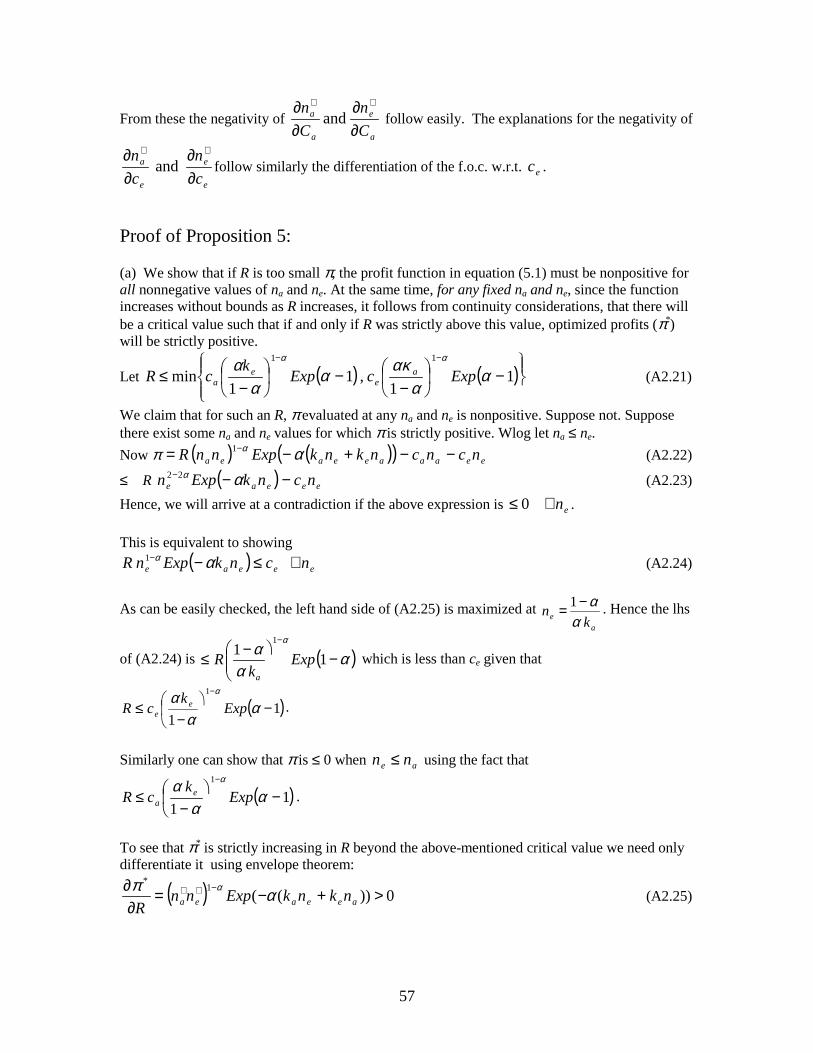
57
From these the negativity of a
e
a
a
Cn
Cn
∂∂
∂∂ ∗∗
and follow easily. The explanations for the negativity of
e
e
e
a
cn
cn
∂∂
∂∂ ∗∗
and follow similarly the differentiation of the f.o.c. w.r.t. ec .
Proof of Proposition 5:
(a) We show that if R is too small π, the profit function in equation (5.1) must be nonpositive forall nonnegative values of na and ne. At the same time, for any fixed na and ne, since the functionincreases without bounds as R increases, it follows from continuity considerations, that there willbe a critical value such that if and only if R was strictly above this value, optimized profits (π*)will be strictly positive.
Let ( ) ( )���
��
���
−��
�
�
−−�
�
�
�
−≤
−−
11
,11
min11
αα
ακαα
α αα
ExpcExpk
cR ae
ea (A2.21)
We claim that for such an R, π evaluated at any na and ne is nonpositive. Suppose not. Supposethere exist some na and ne values for which π is strictly positive. Wlog let na ≤ ne.Now π ( ) ( )( ) eeaaaeeaea ncncnknkExpnnR −−+−= − αα1 (A2.22)
≤ R ( ) eeeae ncnkExpn −−− αα22 (A2.23)Hence, we will arrive at a contradiction if the above expression is en∀≤ 0 .
This is equivalent to showing( ) eeae cnkExpnR ≤−− αα1 en∀ (A2.24)
As can be easily checked, the left hand side of (A2.25) is maximized at a
e kn
αα−= 1 . Hence the lhs
of (A2.24) is ( )ααα
α
−�
���
� −≤−
111
Expk
Ra
which is less than ce given that
( )11
1
−���
�
−≤
−
αα
α α
Expk
cR ee .
Similarly one can show that π is ≤ 0 when ae nn ≤ using the fact that
( )11
1
−���
�
−≤
−
αα
α α
Expk
cR ea .
To see that π* is strictly increasing in R beyond the above-mentioned critical value we need onlydifferentiate it using envelope theorem:
( ) 0))((1*
>+−=∂∂ −∗∗
aeeaea nknkExpnnR
απ α (A2.25)

58
(b) Let φ = ( ) ))((1aeeaea nknkExpnn +−−∗∗ αα
(A2.26)
Now ��
���
∂∂
���
�
�−−+
∂∂
���
�
�−−=
∂∂ ∗
∗
∗
∗
∗
Rn
nRn
nRe
ae
ae
a
ακαακαφπ 112
2
> 0 (A2.27)
0,0 >∂∂>
∂∂ ∗∗
Rn
Rn ea
� . This shows that π* is convex in R.
To see that ∗π asymptotes to a positively sloped line with negative intercept, noticethat the f.o.c.’s can be written as
Rc
kn
ae
a
=�
���
�−−
∗ ααφ 1 (A2.28)
and
Rc
kn
ea
e
=���
���
�−−
∗ ααφ 1 (A2.29)
Now as R increases, na and ne increase (Observation 1). At the same time, since the bracketedquantities in (A2.28) and (A2.29) must always stay positive (as we have argued before),
ea k
nαα−≤ 1* and
ae k
nαα−≤ 1* . Also notice that φ goes to zero only if either na or ne goes to zero
or infinity (this follows from the fact that the function )(1 xkExpx αα −− goes to zero only if eitherx goes to zero or to infinity as can be easily checked). Hence as R goes to zero, it must be the case
that the bracketed terms in (A2.28) and (A2.29) must go to zero. Thus, as ** ,, ea nnR ∞→ go to
critical values ea nn∧∧
, where
ea k
nαα−= 1ˆ (A2.30)
and
ae k
nαα−= 1ˆ (A2.31)
This shows that as ,∞→R π* goes to eeaaaeeaea ncncnknkExpnnR ˆˆ))(()ˆˆ( 1 −−+−− αα . Asa function of R, this is a straight line with positive slope and negative intercept as claimed.
(c) We need to prove
0. <�
���
�
∂∂
∂∂
∗
∗
ππ RRR
(A2.32)
or 2
2
2 ����
�
∂∂<��
����
�
∂∂+
∂∂ ∗∗∗
∗
RR
RR
Rππππ (A2.33)

59
or ( )φφφπππ RR
R <+∂∂ ∗
∗∗
2
2
(A2.34)
or ( )φπφπφπ ∗∗∗∗∗ ++<+∂∂
eeaa ncncR
R (A2.35)
or ( )φφπ ∗∗∗ +<∂∂
eeaa ncncR
R (A2.36)
Now using (A2.28) and (A2.29) to replace ac and ec and using (A2.25), (A2.26) and thedefinition of π*, we see that we need to prove
�
��
�
����
���
�−−−�
��
���
�−−− ∗
∗∗
∗ eae
aea
nkn
Rnkn
RR ααφααφφ 11 RRn
knR
nk
ne
ae
ae
a
���
��
���
∂∂
���
�
�−−+
∂∂
���
�
�−− ∗
∗
∗
∗ααααφ 11*
φααααφ ���
��
���
���
�
�−−+��
�
�
�−−< ∗
∗∗
∗ eae
aea
nkn
nkn
R 11 (A2.37)
Canceling 2φR from both sides, this reduces to proving
���
����
���
−−−��
�
���
−−− ∗
∗∗
∗ eae
aea
nkn
nkn
αααα 111�
���
�
∂∂
���
���
−−+
∂∂
���
���
−−∗
∗
∗
∗
∗ Rn
RknR
nRk
ne
ae
ae
a
αααα 11
�
���
����
���
−−+��
�
���
−−< ∗
∗∗
∗ eae
aea
nkn
nkn
αααα 11 (A2.38)
We now use equations (A2.13) and (A2.14) from the proof of the previous proposition to derive
expressions for Rna
∂∂ *
and Rne
∂∂ *
. As can be easily checked,
∆
����
� −���
���
�−−
=∂∂ ∗∗∗ 2
111 e
eaa nn
RRn
αακα
(A2.39)
and
∆
����
� −���
���
�−−
∗=∂∂ ∗∗∗ 2
111 a
aee nn
RRn
αακα
(A2.40)
where

60
�
��
�
� −−���
���
−−
���
��
�
� −−���
���
−−=∆ ∗∗∗∗ 2
2
2
21111
ea
eae
a nnnk
nαακαααα
211 �
��
����
���
−−
���
���
−−− ∗∗ e
aa
e nnακαακα
(A2.41)
=�
��
�
�
���
���
−���
���
−−−��
�
���
−���
���
−−−��
�
���
−���
���
−∗∗∗∗∗∗ 2
2
2
2
22
111111
aa
eee
aea nk
nnk
nnnαααααααα
(A2.42)
> 0, because of s.o.c.
Using (A2.39) and (A2.40) in (A2.38), the task reduces to proving
�
���
����
���
−−−�
��
���
−−− ∗
∗∗
∗ aae
aea
nkn
nkn
αααα 111
�
��
�
�
���
���
−���
���
−−+��
�
���
−���
���
−∗ ∗∗∗∗ 2
2
2
21111
aa
eee
a nk
nnk
nαααααα
< �
���
����
���
−−+��
�
���
−− ∗
∗∗
∗ eae
aea
nkn
nkn
αααα 11
�
��
�
�
���
���
−���
���
−−−��
�
���
−���
���
−−−��
�
���
−���
���
−∗ ∗∗∗∗∗∗ 2
2
2
2
22111111
aa
eee
aea nk
nnnnnααααακααα
(A2.43)
which holds if
����
� −���
���
�−−+��
����
� −���
���
�−−
∗∗∗∗ 2
2
2
21111
aa
eee
a nk
nnk
nαααααα
�
���
����
���
−−+�
��
���
−−
���
���
−���
���
−< ∗∗
∗∗∗∗ ea
eae
aea
nkn
nknnn
αααααα 111122 (A2.44)
which in turn holds if
�
���
����
���
−−���
���
−−
���
���
−−
���
���
−∗
∗∗∗∗ 22
1111
aae
ae
ae nnk
nk
nnαααααα

61
+ 0111122 <
�
���
����
���
−−���
���
−−
���
���
−−
���
���
−∗
∗∗∗∗
eea
aa
ea nnk
nk
nnαααααα
(A2.45)
which clearly holds.
Proof of Proposition 6:
We write down the Kuhn-Tucker conditions for the optimization problem in (5.8) which arenecessary and sufficient because of concavity of the objective and convexity of the domain.These are:
0)(2 *42
*1
* ≤+−− hvv NmmNmπ (A2.46)
0))(2( **42
*1
* =+−− vhvv NNmmNmπ (A2.47)
0)(2 *42
*3
* ≤+−− vhh NmmNmπ (A2.48)
0))(2( **42
*3
* =+−− hvhh NNmmNmπ (A2.49)
Case A) Suppose 1
42*
*
2)(
mmm
v
h +≤
ππ
or, *42
*1 )(2 vh mmm ππ +≤ (A2.50)
Then *hN must be 0. If not, from (A2.49) we have
0)(2 *42
*3
* =+−− vhh NmmNmπ (A2.51)
and hence *421
*31
*1 )(242 vhh NmmmNmmm ++=π (A2.52)
But from (A2.46),*2
42*
421*
42 )()(2)( hvv NmmNmmmmm +−+≤+ π (A2.53)
Combining (A2.50), (A2.52) and (A2.53), we have*2
42*
31 )(4 hh NmmNmm +< (A2.54)
which is impossible given Min(m1 , m3) > Max(m2 , m4). Hence, ph= 0.
Case C) Suppose )(
2
42
3*
*
mmm
v
h
+≥
ππ
or *3
*42 2)( vh mmm ππ ≥+ (A2.55)
Then *vN must be 0. If not, from (A2.47) we have
*423
*31
*3 )(242 hvv NmmmNmmm ++=π (A2.56)
But (A2.48) gives*2
42*
423*
42 )()(2)( vhh NmmNmmmmm +++≤+ π (A2.57)

62
Combining (A2.55), (A2.56) & (A2.57), we again get a contradiction to the assumption Min(m1 ,m3) > Max(m2 , m4). Hence, ph = 1.
Case B) In this case, it may be checked that
24231
*42
*3*
)(4)(2
mmmmmmm
N hvv +−
+−=
ππ (A2.58)
24231
*42
*1*
)(4)(2
mmmmmmmN vh
h +−+−
=ππ
(A2.59)
satisfy all the K-T conditions.
Furthermore,
*42
*3
*42
*1
*
*
)(2)(2
hv
vh
v
h
mmmmmm
NN
ππππ
+−+−
= (A2.60)
*
*
423
42*
*
1
)(2
)(2
v
h
v
h
mmm
mmm
ππ
ππ
+−
+−= (A2.61)
which is clearly increasing in *
*
v
h
ππ
. Hence ph increases with *
*
v
h
ππ
.
Proof of Proposition 7:
Case A) Suppose 1
4*
*
mm
v
h ≤ππ
or, *4
*1 vh mm ππ ≤ (A2.62)
Then, we claim that *hN must be 0. Suppose not. Then, in the horizontal factor market, price of
the factor must equal *hπ (to prevent further entry), while in the vertical factor market the price
must be greater than or equal to *vπ (thus allowing for the possibility that no vertical show is
organized). These considerations yield the following two equations:
*4
*3
*vhh NmNm +=π (A2.63)
*2
*1
*hvv NmNm +≤π (A2.64)
Multiplying (A2.63) by m1 and (A2.64) by m4 and using (A2.62) we see that

63
*42
*41
*41
*31 hvvh NmmNmmNmmNmm +≤+ (A2.65)
But the above contradicts Min(m1 , m3) > Max(m2 , m4). Hence *hN must be 0 and so should ph.
Case C) The proof of this is similar to that of case A. Now, *vN must be zero; otherwise
equality between factor cost and revenues must hold in the vertical market while factor costshould be at least as large as revenues in the horizontal market. These, along with the stated
condition 2
3*
*
mm
v
h ≥ππ
will then generate a contradiction to the assumption Min(m1 , m3) > Max(m2 ,
m4).
Case B) We argue that in this case both *vN and *
hN must be strictly positive. Clearly, bothcannot be zero, or entry will occur in both horizontal and vertical arena. Under the statedconditions, it is also impossible to have one of them assume zero value and the other a positivevalue. Suppose, for instance, *
vN is zero, while *hN is positive. Then,
We must have:
*2
*hv Nm≤π (A2.66)
and*
3*
hh Nm=π (A2.67)
From the above two equations we get 2
3*
*
mm
v
h ≥ππ
, which contradicts the stated assumption for this
case. Similarly, we can disprove the possibility that *hN is zero while *
vN is positive. Given thepositivity of both, we can use the equality of revenue and costs in both markets to write:
*2
*1
*hvv NmNm +=π (A2.68)
and*
4*
3*
vhh NmNm +=π (A2.69)
These can be solved to obtain
4231
*2
*3*
mmmmmm
N hvv −
−=
ππ (A2.70)
4231
*4
*1*
mmmmmm
N vhh −
−=
ππ (A2.71)
Hence,
*
*
23
4*
*
1
*
*
v
h
v
h
v
h
mm
mm
NN
ππ
ππ
−
−= (A2.72)

64
As the above expression clearly increases with the *
*
v
h
ππ
ratio, so must ph.
Appendix 3 (Proofs of All Results in Section 6)
First, we state a few useful facts which we will use in the proofs that follow.
Fact 1. Let αα
αα
21211
1 −−−
+= cbA (A3.1)
and αα
αα
211
211 −−
−+= cbB (A3.2)
(Recall: xyb ββ= , xyc γγ= ).
Then α
α
α
α
γβA
BBAR xxH
−−
+=11
Proving this is a simple matter of manipulating the expression for Rh in (5.3).
Fact 2.
∈A (1, 2); ∈B (1, 2).
This follows from ∈b (0, 1) and ∈c (0, 1).
Fact 3.
BAcb ≥↔≥
This follows trivially from the definitions of A and B.
Fact 4.
AcbBcb ≥↔≥
This follows since αα
αα
211
211
−−
−−
+= cbbbB& α
ααα
211
211
−−
−−
+= cbcAc
Fact 5.
αα−<= 1
,, ABMax
BAMax
cbcb

65
Proof. Given that αα
αα
21211
−−−
> bb , clearly to maximize BA , c should be set at 1. Now, the f.o.c.
for this maximization problem gives .1 bBA
αα−= Since, b 1< , the result follows.
Proof of Observation 2:
We separately deal w/ the cases i) xx γβ = , ii) cb = and iii) .0))(( >−− cbxx γβ
Case i) In this case xvR β2= & �
���
�+=
−−
α
α
α
α
βA
BBAR xH
11
Hence it suffices to show 211
>+−−
α
α
α
α
AB
BA
(A3.3)
or to show αα BABA 2>+ (A3.4)But 2
12
12 BABA ≥+ (A3.5)1>A� , 1>B (Fact 2), 2
1<α , it follows that αα BABA >21
21
. Hence proved.
Case ii) Suppose b = c
In this case ( ) ( ) αααα γβ
2121211
211
11−−
−− +++= bbR xxH (A3.6)
( ) ααγβ
21211
1)(−
−++= bxx (A3.7)whereas xxvR γβ += (A3.8)
Hence it suffices to show ( ) 1121
211
>+−
−α
αb , which of course, holds since 21<α .
Hence proved.
Case iii) We deal with the situation where xx γβ > and cb >The argument is symmetric in the case xx γβ < & cb < .
If xx γβ > & cb > , it follows that
vxxxxH RA
BBAR =+>+=
−−
γβγβ α
α
α
α 11
(A3.9)
iff �
��
�−>�
���
�−
−−
α
α
α
α
γβA
BBA
xx
11
11 (A3.10)
(A3.10) follows if we can show
a) 011
>−−
α
α
BA
(A3.11)
& b) α
α
α
α
AB
BA −−
−>−11
11 (A3.12)

66
b) has already been shown to hold in dealing with Case i).a) also holds BAcb >>� (Fact 3) and 1>A (Fact 2). Hence proved.
Now note that in each case, we have shown that under the stated conditions Rh strictly exceeds Rv.Hence, appealing to the continuity of the Rh & Rv functions (of their arguments b, c, xβ , xγ – aslong as they are strictly positive) we see that the inequality continues to hold in a nbd. of the setof parameters satisfying eqn. (6.2).
Proof of Proposition 8:
We show that 0>∂∂
bRh under the stated condition. The positivity of
cRh
∂∂
follows
symmetrically. Now,
��
���
��
�
�
−−�
�
�
�
−−−=
∂∂
−−
−−
−− −−−−− αα
αα
αα
αα
ααα
αααβ αααα 21
121
132121
21211)1( 11 cbABcbAB
bR
xh
��
���
��
�
�
−−−�
�
�
�
−−+ −−−
−−−
−−−−− αα
αα
αα
αα
ααα
αααγ αααα 212121
121
13
211
21)1( 11 cbABcbABx (A3.13)
Case i) cb =
If cb = , BA = . Then,
021
)1(21
)1(2121
)1( 222 21
2
>�
��
���
��
−−−
−−+�
�
��
−−
−−=
∂∂
−−
ααα
αααγ
αα
ααβα
ααxx
h bAb
R (A3.14)
Case ii) xx γβ =
To show:αα
αα
αα
αα αααα αα 21
121
132121 1122)1( −
−−−
−− −−−−− −− cbABcbAB
0)1()1( 2121211
2113 11 >−−−+ −−−
−−−
−−−−− αα
αα
αα
αα αααα αααα cbABcbAB (A3.15)
or equivalently,
0)1()1()1( 22 >−−−+−−AB
bc
bc
BA αααααα (A3.16)
But � αα−< 1max
BA
and αα−< 1max
AB
(Fact 5), it suffices to show:
0)1()1()1(1)1( 22 ≥−−−−+⋅−−−αααααα
αααα
bc
bc
(A3.17)
which, of course is true.
Case iii) 0))(( >−− cbxx γβ

67
Suppose cb < & xx γβ < . We need to show
��
��� −−−>�
�
��� −− −
−−−
−−
bc
ABcb
BbAc
bccb xxxx
22 )1()1()1( 2113
211
2121 αβααγαβααγ αα
αα
αα
αα
(A3.18)
Now if cb <α
ααα
αα
αα
2113
211
2121 −−
−−
−− > cbcb (A3.19)and if xx γβ < additionally
BbAc
bc
xx2)1( αβααγ >− (A3.20)
and finally →< cb AB
bc > allows us to claim
bc
BA
AB
bc
bc
xxxx22 )1()1()1( αβααγαβααγ +−>−+− (A3.21)
Combining (A3.19), (A3.20), and (A3.21), (A3.18) is seen to follow.The case of cb > & xx γβ > is similar and omitted.
Proof of Proposition 9:
Suppose βx = γx. Then,
αα
αα
αα
αα
ααα
ααα αααα 21
1321
121
121
13
2121[sgn]sgn[ 1111 −
−−−
−−
−− �
��
�
−+�
���
�
−−=
∂∂
−∂∂ −−−−− cbABcbAB
cR
bR hh
αα
αα
αα
αα
ααα
ααα αααα 212121
121
13
211
21)1( 11 −−−
−−− �
��
�
−−−
−−+ −−−−− cbABcbAB
]21
121
)1(212121
1321
111 α
αα
αα
ααα
ααα
ααα αααα −−−
−−−
��
��
�
−−−
−−− −−−−− cbABcbAB (A3.22)
The sign of the above expression on the other hand, is the same as that of
��
� −+�
�
� −−−�
�
� −−
BbAc
AcBb
BA
cb
AB
bc ααα )1()1( (A3.23)
Clearly this is 0 if cb = when BA = and BbAc = .
Now suppose cb > . Then (A3.23) can be written as
AbBcAcBbAcBb
AbBcBcAbAcBb ))(())(()1( +−++−−− αα (A3.24)

68
Noting that AcBbBcAb +>+ ( cBAbBA )()( −>−� ) and αα >− )1( , this is clearly
seen to be negative. The negativity of b
Rc
R hh
∂∂
−∂∂
when bc > follows analogously.
To see 0=∂∂
−∂∂
cR
bR hh when b = c, one simply needs to look at expression (A3.14) where we
have computed b
Rh
∂∂
. Noting that c
Rh
∂∂
can be obtained from this expression by replacing b by c
and A by B and since A = B when b = c, the result follows.
Finally, we show that when b ~ c:
> cb 0<∂∂
−∂∂
cR
bR hh (A3.25)
and < cb 0>∂∂
−∂∂
cR
bR hh (A3.26)
Since, 0=∂∂
−∂∂
cR
bR hh when b = c, this is achieved by showing that the function Rh is concave
in δ for δ small when b is replaced by e + δ and c by e - δ and e is arbitrary.
Now ),,(),,( 21 δαγδαβ eReRR xxh += where
α
αα
αα
α
αα
αα
δδ
δδδα
���
�−++
��
��
�−++
=−−
−
−
−−−
211
21
1
21211
1
)()(1
)()(1),,(
ee
eeeR (A3.27)
and
α
αα
αα
α
αα
αα
δδ
δδδα
���
�−++
��
��
�−++
=−−
−
−
−−
−
21211
1
211
21
2
)()(1
)()(1),,(
ee
eeeR (A3.28)
Tedious differentiation and some manipulations show that the second derivative of both R1 and R2
evaluated at δ = 0 is )21(211
11
2)1(2 αααα +−−−
+−+− ee which is negative. Hence...
Proof of Proposition 10:
By looking at expressions (5.2) and (5.3) one can see that if all product evaluation parameterswere to experience a lowering of r % because of a decrease in the transaction intensity factor,then both Rv and Rh will go down by r %. We need to prove that this will raise the **
vh ππ ratio.

69
This will hold if 0)()(
1*
*
<�
���
�
∂∂
=rv
h
rRrR
r ππ
(A3.29)
which in turn holds if v
v
hh
h
v RR
RRR
RRR ∂
∂<∂∂ *
**
* )()( ρπππ (A3.30)
Or, if the elasticity of the *π function at Rh is less than the corresponding elasticity at Rv. But ifvh RR > , this will hold according to part (c) of Proposition 5.
Proof of Lemma 1:
Recalling that α
α
α
α
γβA
BBAR xxH
−−
+=11
where αα
αα
21211
1 −−−
+= cbA and αα
αα
211
211 −−
−+= cbB , we
obtain by direct differentiation
��
���
∂∂+�
�
���
∂∂=
∂∂ −−
α
α
α
α
αγ
αβ
α AB
BAR
xxH
11
(A3.31)
α
αααα
αα
αα
β 2
11)1(
B
BBAAABx
∂∂−
∂∂−
=
−−−
α
αααα
αα
αα
γ 2
11)1(
A
AABBBAx
∂∂−
∂∂−
+
−−−
(A3.32)
Now to calculate α∂∂A
, we note that αα
αα
21211
1 −−−
=− cbA (A3.33)
and hence ln cbA ln21
ln21
1)1(α
ααα
−+
−−=− (A3.34)
Differentiating both sides w.r.t. α we get
cbAA ln
)21(1ln
)21(1
1 22 ααα
−+
−=
−∂∂
(A3.35)
which gives ( ) 2)21(lnln
21211
ααα
ααα
−+=
∂∂
−−− cbcbA
(A3.36)
Similarly ( ) 2)21(lnln
211
21
αααα
αα
−+=
∂∂
−−
−cbcbB
(A3.37)
Using (A3.36) and (A3.37), (A3.32) can be written as

70
[ ]{ αα
αα
αα
αα αααα ααβ
αα21
1212121
111
2 )1()21(
lnln−−
−−−−
−−−−− −−−+=
∂∂
cbBAcbABcbRx
h
[ ] }αα
αα
αα
αα αααα ααγ 2121
121
121 11)1( −−
−−−
− −−−−− −−+ cbABcbBAx (A3.38)
or ��
���
��
�
� −−+���
� −−−+=
∂∂
−−−−
ABbc
BAcbcbABcbR
xxh ααγααβ
ααα
αα
ααα )1()1()21(
lnln2121
2 (A3.39)
Now since 0lnln <+ cb ( 1<b , 1<c ), it follows that 0<∂∂α
hR if the curly bracketed term
above is positive.
To show that this holds under (6.2), we consider the 3 cases i) cb = ii) xx γβ =and iii) 0))(( >−− cbxx γβ separately.
Case i) When cb = , BA = & the curly bracketed term reduces tobb xx )21()21( αγαβ −+− ; which is clearly positive.
Case ii) Here, we need to show�
��
� +>+− bABc
BAcb αα ))(1( (A3.40)
which holds if bABc
BAcb +≥+ (A3.41)
or if 0)( ≥���
� −−Bc
AbBA (A3.42)
or if 0))(( ≥−− AcbBBA (A3.43)
This holds since if cb ≥ , BA ≥ and AcbB ≥ (Facts 3 and 4) while if cb ≤ ,BA ≤ and AcbB ≤ .
Case iii) ��
��� −−+�
�
��� −−
ABbc
BAcb xx
ααγααβ )1()1(
���
���
�� −+�
�
�� −≥
ABbc
BAcb xx γβ
21
(A3.44)
Now suppose cb > and xx γβ > . Then the given expression is
���
� −+−≥A
bBAcB
AcbBxγ2
1
0)(21 ≥���
� −−≥AB
BAAcbBxγ (A3.45)

71
The case cb < & xx γβ < follows similarly.
Proof of Lemma 2:
We write the linear approximation of π*(R) as m(α) R +c (α), where m is the slope and c is theintercept – both of which are functions of α (they are functions of other parameters too, but notexplicitly stated as such since we deal with changes in α only in this lemma).From the discussion in Section 5.A, on replacing the expressions for an̂ and en̂ in the asymptoteto π* we observe that:
α
ααα
−�
���
���
��
−=1
2
2 11)(ekk
mea
(A3.46)
���
� −−=����
� −���
���
�+−=
αα
ααα 11)( A
kc
kc
ca
e
e
a (A3.47)
where A is a constant independent of α.
Now, let )()()(and)()()( 2*21
*1 αααπαααπ cRmcRm +=+= . We need to show that
0)()(
*2
*1 <
����
�
∂∂
απαπ
α under the stated assumptions.
(A3.48)Now note that
(A3.49)
Since R1 > R2 , we will have proven the desired result if we can show that the intercept is more
elastic to changes in α than the slope is (note that a rise in α lowers both). Or if,
)()(
)()(
αα
αα
mm
cc ′
<′
(A3.50)
Taking log of (A3.46) and differentiating w.r.t. α gives us the l.h.s. of (A3.50):
( )αα −−
11 (A3.51)
Similarly, taking log of (A3.45) and differentiating w.r.t. α gives us the r.h.s. of (A3.50):
( )( ) ( )( )[ ])()()()()()()()(sgn)()(sgn 2112*
2
*1 αααααααααπαπ
αcRmcRmcRmcRm −′−−−′−=
�
���
����
���
∂∂
( )( )[ ])()()()(sgn)()(
sgn 21*2
*1 αααααπαπ
αmccmRR ′−′−=
���
����
���
∂∂

72
���
� +−−−−−α
αα 22)ln(ln2)1ln(2 eakk (A3.52)
Now, if kake < e-2, then (A3.51) will be smaller than (A3.52) if the following hold:
)1(12andln2)1ln(2ααα
αα−
>>− . But both inequalities clearly hold since α is less than
½.
Proof of Proposition 11:
Suppose αlo < αhi. By Lemma 2, );(
));(();(
));((*
*
*
*
lov
loloh
hiv
hiloh
RR
RR
απααπ
απααπ
> (note that Rv does not
depend on α). Also by Lemma 1, and the increasing-ness of the π* function , we have
);());((
);());((
*
*
*
*
hiv
hiloh
hiv
hihih
RR
RR
απααπ
απααπ
> . Combining these, yields the desired result.