Algebras de Clifford - Parte 5 - Los Grupos Asociados a Las Algebras de Clifford

A Theory of Neural Computation
with
Clifford Algebras
Dissertation
zur Erlangung des akademischen Grades
Doktor der Ingenieurwissenschaften
(Dr.–Ing.)
der Technischen Fakultat
der Christian-Albrechts-Universitat zu Kiel
Sven Buchholz
Kiel
2005

1. Gutachter Prof. Dr. Gerald Sommer (Kiel)
2. Gutachter Prof. Dr. Reinhold Schneider (Kiel)
3. Gutachter Prof. Dr. Thomas Martinetz (Lubeck)
Datum der mundlichen Prufung: 16.03.2005

Abstract
The present thesis introduces Clifford Algebra as a framework for neural compu-
tation. Clifford Algebra subsumes, for example, the reals, complex numbers and
quaternions. Neural computation with Clifford algebras is model–based. This
principle is established by constructing Clifford algebras from quadratic spaces.
Then the subspace grading inherent to any Clifford algebra is introduced, which
allows the representation of different geometric entities like points, lines, and so on.
The above features of Clifford algebras are then taken as motivation for introducing
the Basic Clifford Neuron (BCN), which is solely based on the geometric product of
the underlying Clifford algebra. Using BCNs the Linear Associator is generalized
to the Clifford associator. As a second type of Clifford neuron the Spinor Clifford
Neuron (SCN) is presented. The propagation function of a SCN is an orthogonal
transformation. Examples of how Clifford neurons can be used advantageously
are given, including the linear computation of Mobius transformations by a SCN.
A systematic basis for Clifford neural computation is provided by the important
notions of isomorphic Clifford neurons and isomorphic representations. After the
neuron level is established, the discussion continues with (Spinor) Clifford Multi-
layer Perceptrons. The treatment is divided into two parts according to the type
of activation function used. First, (Spinor) Clifford Multilayer Perceptrons with
real–valued activation functions ((S)CMLPs) are studied. A generic Backpropaga-
tion algorithm for CMLPs is derived. Also, universal approximation theorems for
(S)CMLPs are presented. The efficency of (S)CMLPs is shown in a couple of sim-
ulations. Finally, the class of Clifford Multilayer Perceptrons with Clifford–valued
activation functions is studied.

ii

Acknowledgments
The making of this thesis would not have been possible without the support of a
lot of people. It is my great pleasure to thank them here.
First of all I thank my supervisor Professor Gerald Sommer for his confidence in
my work and for the encouraging discussions during all the years. From the very
first ideas to this final version of the text he has been a constant source of advise
and inspiration.
I also thank the co–referees Professor Thomas Martinetz and Professor Reinhold
Schneider for their interest in my work and their helpful comments.
Furthermore, I thank all members of the Cognitive Systems Group, Kiel for their
support and help. My very special thanks go to Vladimir Banarer, Dirk Kukulenz,
Francoise Maillard, Christian Perwass and Nils Siebel.
Last, but not least, I thank my parents Claus and Jutta, to whom I dedicate this
thesis.
iii

iv

Contents
1 Introduction 1
1.1 Motivation . . . . . . . . . . . . . . . . . . . . . . . . . . . . . . . . . . 1
1.2 Related Work . . . . . . . . . . . . . . . . . . . . . . . . . . . . . . . . 4
1.3 Structure of the Thesis . . . . . . . . . . . . . . . . . . . . . . . . . . . 5
2 Clifford Algebra 7
2.1 Preliminaries . . . . . . . . . . . . . . . . . . . . . . . . . . . . . . . . . 8
2.2 Main Definitions and Theorems . . . . . . . . . . . . . . . . . . . . . . 13
2.3 Isomorphisms . . . . . . . . . . . . . . . . . . . . . . . . . . . . . . . . 18
2.4 The Clifford Group . . . . . . . . . . . . . . . . . . . . . . . . . . . . . 21
3 Basic Clifford Neurons 25
3.1 The 2D Basic Clifford Neurons . . . . . . . . . . . . . . . . . . . . . . 30
3.1.1 The Complex Basic Clifford Neuron . . . . . . . . . . . . . . . 31
3.1.2 The Hyperbolic Basic Clifford Neuron . . . . . . . . . . . . . . 34
3.1.3 The Dual Basic Clifford Neuron . . . . . . . . . . . . . . . . . 38
3.2 Isomorphic BCNs and Isomorphic Representations . . . . . . . . . . 41
3.2.1 Isomorphic Basic Clifford Neurons . . . . . . . . . . . . . . . . 41
3.2.2 Isomorphic Representations . . . . . . . . . . . . . . . . . . . . 45
3.2.3 Example: Affine Transformations of the Plane . . . . . . . . . 48
v

CONTENTS
3.3 The Clifford Associator . . . . . . . . . . . . . . . . . . . . . . . . . . . 50
3.4 Summary of Chapter 3 . . . . . . . . . . . . . . . . . . . . . . . . . . . 53
4 Spinor Clifford Neurons 55
4.1 The Quaternionic Spinor Clifford Neuron . . . . . . . . . . . . . . . . 57
4.2 Isomorphic Spinor Clifford Neurons . . . . . . . . . . . . . . . . . . . 61
4.3 Linearizing Mobius Transformations . . . . . . . . . . . . . . . . . . . 65
4.4 Summary of Chapter 4 . . . . . . . . . . . . . . . . . . . . . . . . . . . 70
5 Clifford MLPs with Real–Valued Activation Functions 71
5.1 Backpropagation Algorithm . . . . . . . . . . . . . . . . . . . . . . . . 74
5.2 Universal Approximation . . . . . . . . . . . . . . . . . . . . . . . . . 79
5.3 Experimental Results . . . . . . . . . . . . . . . . . . . . . . . . . . . . 84
5.3.1 2D Function Approximation . . . . . . . . . . . . . . . . . . . 84
5.3.2 Prediction of the Lorenz Attractor . . . . . . . . . . . . . . . . 96
5.4 Summary of Chapter 5 . . . . . . . . . . . . . . . . . . . . . . . . . . . 102
6 Clifford MLPs with Clifford–Valued Activation Functions 105
6.1 Complex–Valued Activation Functions . . . . . . . . . . . . . . . . . . 106
6.2 General Clifford–Valued Activation Functions . . . . . . . . . . . . . 112
6.3 Experimental Results . . . . . . . . . . . . . . . . . . . . . . . . . . . . 116
6.4 Summary of Chapter 6 . . . . . . . . . . . . . . . . . . . . . . . . . . . 117
7 Conclusion 119
7.1 Summary . . . . . . . . . . . . . . . . . . . . . . . . . . . . . . . . . . . 119
7.2 Outlook . . . . . . . . . . . . . . . . . . . . . . . . . . . . . . . . . . . . 121
A Supplemental Material 123
vi

CONTENTS
A.1 Dynamics of the Linear Associator . . . . . . . . . . . . . . . . . . . . 123
A.2 Update Rule for the Quaternionic Spinor MLP . . . . . . . . . . . . . 126
A.3 Some Elements of Clifford Analysis . . . . . . . . . . . . . . . . . . . 127
vii

CONTENTS
viii

Chapter 1
Introduction
The three stages of intelligent action according to [22] are conversion of the stimu-
lus into an internal representation, manipulation of that representation by a cogni-
tive system to produce a new one, and conversion of that new representation into a
response. This clearly maps well onto (feed–forward) neural networks. However,
such networks rather process unstructured data than structured representations.
Many problems arise from that lack of structure, most important the integration of
prior knowledge. This thesis introduces Clifford Algebra as a framework for the
design of neural architectures processing representations advantageously.
1.1 Motivation
Thinking about mind, consciousness, and thinking itself is the root of all philoso-
phy. Therefore philosophy was the first discipline challenging the question
What is intelligence?
In the first half of the 20th century other disciplines started their own challenge
of particular versions of the above question. Each one driven by its own special
origins, methods and hopes.
A psychological approach was undertaken in 1938 by Skinner. In [81] he showed
how the environment could be used to train an animal’s behavior. A refinement of
that principle, reinforcement learning, is widely used today for mobile robots and
multi–agent systems [43].
1

1.1 MOTIVATION
Already in 1933 Thorndike presumed [85] that learning accounts in the brain by
the change of connectivity patterns among neurons. For this postulated principle
he had coined the term connectionism. Some years later Hebb reported in [35] bi-
ological evidence for connectionism. From brain slice experiments he inferred the
following rule: If two neurons on either side of a synapse (i.e. connection) are ac-
tivated simultaneously, then the strength of that synapse is selectively increased.
This can be seen as the offspring of unsupervised learning, which is the general
theory of learning without (external) feedback (from a teacher).
Meanwhile the seeds of a new era were sown. Many mathematicians were chal-
lenged by Hilbert’s Entscheidungsproblem
What are the intuitively computable functions?
The work of Church [17] and Kleene [46] cumulated in 1936 in what is now famous
as the Church thesis: The computable functions are the general recursive function. In the
same year Turing proposed in his famous paper [86] a hypothetical device capable
of computing every general recursive function.
Inspired by both neurophysiology and Turing’s work McCulloch and Pitts pub-
lished in 1943 a highly influential paper [58]. Their idea was to view biological
neurons as sort of logical gates. Thus way biological neurons were ”turned into”
processing units for the first time. This was the birth of neural computation — a
biologically inspired paradigm for computation.
Well, there was another computational model which also emerged in that period
of time. That is of course the computer itself. When the computer era started in the
1950s neural computation was one of the first research fields participating from its
benefits. Computers allowed for simulation of neural models, for which [28] is a
very early example.
The next milestone in neural computation was set in 1958 when Rosenblatt [72] pro-
posed a neural architecture that he called Perceptron. The Perceptron was intended
as a model for human perception and recognition. Later in [73] he introduced as
modification an error correction procedure for it. Learning by error correction is
termed supervised learning. Perceptrons created much excitement and interest in
neural computation. Neural networks like Perceptrons seemed to deliver what
Turing once defined to be the creative challenge of artificial intelligence (AI) [21]
What we want is a machine that can learn from experience.
2

CHAPTER 1. INTRODUCTION
That interest was abruptly stopped at the end of the 1960s. Whether this was
caused by the 1969 book Perceptrons [59] by Minsky and Papert has been a con-
troversial question ever since. The book contained many examples for the limited
power of single Perceptrons, among them the famous exclusive–or (XOR) prob-
lem. For Perceptrons with several layers an efficient learning procedure was still
not known at that time. It was not until the mid 1980s that neural networks trained
by supervised learning entered the stage again. But this time it meant a real revo-
lution.
That new chapter in the history of neural computation is attributed with the names
of Rumelhart and McClelland [77, 57]. One particular contribution by these au-
thors [76] introduced an error correction procedure for multi–layer neural net-
works. Since then the procedure is known as Backpropagation and the associated
network as Multilayer Perceptron (MLP). The MLP soon turned out to be very pow-
erful for almost any type of applications. Theoretically, it was proven to be able to
learn any reasonable function [23]. Around that time neural networks were widely
recognized as leading directly towards real artificial intelligence. Or, as stated in
[34]
The neural network revolution has happened. We are living in the aftermath.
That statement remains true. However, many of the enthusiasm originally directed
to neural networks seems to be gone today. Sure, like everything else, science
has its modes. But there are better optimization techniques than Backpropaga-
tion. Learning from examples has theoretical bounds — one being the so-called
bias/variance dilemma [31]. New players have entered the scene - like Support Vector
Machines [88] or approximative algorithms. So, has neural computation lost itself
in too many technical details? Of course, neural networks are well established and
things are still away from a crisis. Nevertheless some important roots seem fallen
into oblivion. Those being the cognitive ones, i.e. representational aspects.
Cognitive science studies the processes and representations underlying intelligent
action. One particular question arising is
How can it be that a representation means something for the cognitive systems itself?
We believe that this question , although casted very philosophically, is of high rel-
evance for neural computation. The integration of prior knowledge is the widely
accepted ”solution” to the bias/variance dilemma mentioned above. However,
3

1.2 RELATED WORK
this requires nothing less than to solve the representation problem — how to en-
code knowledge. If one wants to come up with a fairly general solution one has to
tackle the previous question.
From the system design perspective this calls for an appropriate mathematical
framework. Here we propose Clifford algebra which allows the processing of geo-
metric entities like points, lines and so on. It is a very efficient language for solving
many tasks connected to the design of intelligent systems [24, 74, 82]. To establish
the theory of Clifford neural computation from the outlined motivation as a pow-
erful model–based approach is the main goal of this thesis. We will start with the
design of Clifford neurons for which weight association is interpretable as a geo-
metric transformation. Then it is demonstrated how different operation modes of
such neurons can be selected by different data representations. From the neuron
level we then proceed to Clifford Multilayer Perceptrons.
1.2 Related Work
Technically speaking, a Clifford algebra is a generalization of complex numbers
and quaternions. Neural networks in such domains are not new. The history of
complex neural networks already started in 1990 with a paper by Clarke [18]. Soon
this was followed by Leung and Haykin [54] presenting the complex Backpropaga-
tion algorithm. The most influential paper was published by Georgiou and Kout-
sougeras [32] in 1992. Therein the topic of suitable activation functions for Complex
Multilayer Perceptrons was discussed for the first time. In particular, Georgiou and
Koutsougeras proved a list of requirements that complex–valued activation func-
tions have to fulfill in order to be applicable. Unfortunately, the complex version
of the standard sigmoidal activation function mostly used in the real MLP was ex-
cluded by those requirements. Another rather trivial complex–valued activation
function ( z1+|z|
) was proposed, and, also the use of real–valued activation functions
for Complex MLPs was suggested in this paper. In 1995 Arena et al. [2] proved the
universal approximation property of a Complex MLP with real sigmoidal activa-
tion function. They also revealed drawbacks of the only known complex activation
function proposed in [32]. Complex MLPs with real–valued activation became the
standard notion of complex neural networks, and complex neural computation re-
mained unattractive for most researchers.
Meanwhile Clifford neural networks had entered the stage. Pearson [62] intro-
duced Clifford MLPs utilizing a Clifford version of the complex activation function
4

CHAPTER 1. INTRODUCTION
from [32]. The same function claimed to be useless by Arena et al. a year later. In
1997 Arena et al. introduced the Quaternionic MLP, a MLP formulated in terms of
quaternions using real–valued activation functions again. The same year saw a pa-
per of Nitta [61] on Complex MLPs which did not add anything new to the case. A
new attempt to vitalize complex–valued activation functions was started recently
by Kim and Adali [44].
Most of the above mentioned literature will be reviewed in this thesis. Clifford
MLPs with both real–valued and Clifford–valued activation functions will be stud-
ied for algebras not considered before in the literature. Moreover, new propagation
functions for Clifford MLPs will be presented. However, all this is not the main
goal of this thesis, it results from it. As outlined in the previous section, this thesis
tries to establish Clifford neural computation as a generic model–based approach
to design neural networks capable of processing different geometric entities. In
particular, data is not viewed as ,say, complex numbers, but as points in the plane.
Consequently, a Complex MLP is viewed as transforming such data in some certain
geometric way. That way we will have a new, different and unified look at those
networks. In that sense, also work like [16, 29] can be seen as roughly related.
Closely related is the work of our colleague V. Banarer [5, 4, 64]. However, his work
focuses on classification and practical applications.
1.3 Structure of the Thesis
After this introduction the thesis starts with an outline of Clifford algebra in chap-
ter two. The material is presented in a self–contained way. Special emphasis is
given to the geometric interpretation of the algebraical framework. In particular,
the Clifford group is studied which acts as geometric transformation group on dif-
ferent geometric entities. The insights gained are then directly used for the design
and motivation of Clifford neurons in the two subsequent chapters.
Chapter three introduces neurons based on one single geometric product, which
are the atoms of all Clifford neural computation. Many illustrations for the model–
based nature of Clifford neurons are worked out. A complete overview over the
two–dimensional case in terms of algorithms and dynamics is given. The funda-
mental topic of isomorphic Clifford neurons and isomorphic representations is also
covered in detail. Finally, a linear architecture utilizing a line representation for Eu-
clidean transformations of the plane is presented.
5

1.3 STRUCTURE OF THE THESIS
The fourth chapter is devoted to Clifford neurons based on two geometric prod-
ucts that perform orthogonal transformations on arbitrary geometric entities by
mimicking the operation of the Clifford group. Efficient learning algorithms for
such neurons are derived. As a representative of that class of Clifford neurons the
Quaternionic Spinor Neuron is studied in detail. Again, a discussion of isomor-
phic issues is provided. In the last section of the chapter an architecture linearizing
the computation of Mobius transformations is introduced. For this architecture a
conformal embedding of the data is utilized.
Based on the methodical and algorithmical foundations of chapter three and four
the thesis proceeds with the study of Clifford Multilayer Perceptrons. The focus
thereby is set to the topic of function approximation. According to the type of
activation functions used the material is divided into two separate chapters.
Clifford Multilayer Perceptrons with real–valued activation functions are studied
in chapter five. The chapter begins with reviewing the literature on the subject in-
cluding the complex and quaternion case. The architecture is then generalized to
arbitrary Clifford algebras and also extended to networks based on the new neu-
rons developed in chapter four. Universal approximation is proved for all new
derived networks with underlying Clifford algebras up to dimension four. The
chapter concludes with an extensive section of experiments comparing the perfor-
mance of the architectures known from the literature with the new developed ones.
Chapter six deals with Multilayer Perceptrons with Clifford–valued activation func-
tions. In contrast to the architectures of chapter five real analysis is no longer suf-
ficient for the mathematical treatment of such networks. The case of complex–
valued activation functions is examined first using the available literature. Then
the theory of hyperbolic–activation functions is developed. Analysis in higher di-
mensional Clifford algebras is still an ongoing field of mathematical research rather
than an established theory. Therefore, the topic of general Clifford–valued activa-
tion function is only outlined.
Each of the chapters three to six cover one particular Clifford neural architecture.
Therefore all of them are provided with an individual summary. The thesis con-
cludes with chapter seven, which reviews the proposed methods and obtained re-
sults upon the whole. The benefits of the chosen approach, but also open problems
and directions for further work are discussed.
Part of the work in this thesis has been presented in the following publications
[11, 12, 13, 14, 15].
6

Chapter 2
Clifford Algebra
Clifford algebras are named after the British mathematician William K. Clifford. In
the 1960s David Hestenes started to extend Clifford Algebra with geometric con-
cepts. His broader mathematical system is nowadays known as Geometric Alge-
bra, a term originally coined by Clifford himself.
This introductory chapter on Clifford Algebra has the following structure. Al-
though the definition of an algebra is pretty much common knowledge, that will
be exactly our entrance into the world of Clifford Algebra. This is simply due to
the fact that there is no better way to understand what a (Clifford) algebra is all
about. A vector space is endowed with an additional structure by introducing a
product on it.
After reviewing some basic facts about algebras and rings we proceed by looking
at complex numbers and quaternions as algebras. That way the generalization
to Clifford algebras is prepared. The distinguished role of complex numbers and
quaternions is well pointed out by recalling a famous theorem of Frobenius.
Then the main definition and theorems of Clifford algebras will be presented fol-
lowing mostly the books by Porteus [67] and Lounesto [56]. By doing so Clifford
algebras will be constructed from quadratic spaces, and, hence, will have a metric
structure right from the beginning1. The two–dimensional Clifford algebras will
be studied in greater detail including the only degenerate algebra concerned in
this thesis. In the last section of the chapter the Clifford group is introduced which
1There is and will always be an ongoing discussion in the Clifford (Geometric) Algebra com-
munity, if this is a good idea and how important metric aspects are for the very first foundation
of Clifford (Geometric) Algebra [40]. For our approach, since being heavily based on the idea of
transformation groups, they are mandatory.
7

2.1 PRELIMINARIES
will provide a first geometrical interpretation for many of the Clifford neural archi-
tectures developed later then.
The mathematical material is presented in a self–contained way. Since we believe
that the theory of Clifford neural computation is in large parts an algebraic theory,
algebraic aspects are the focus of this introduction. For a more geometrical intro-
duction to Clifford (Geometric) Algebra we refer to the original work of Hestenes
[39, 40].
2.1 Preliminaries
To begin at the beginning, let us start with the definition of a real algebra.
Definition 2.1 (Real Algebra) A real algebra is a real linear space (A,+, ·) endowed
with a bilinear product
⊗ : A×A → A, (a, b) 7→ a⊗ b .
Hence, a real algebra is a pair ((A,+, ·),⊗) .
Since we only consider real algebras throughout this thesis, we shall often speak
loosely of algebras hereafter. Also, when there is no danger of confusion, we will
just write ab instead of a⊗ b in order to shorten expressions.
An algebra may, or may not, have the following additional properties.
Definition 2.2 (Types of Algebras) An algebra ((A,+, ·),⊗) is called
(i) associative, if for all a, b, c ∈ A : (a⊗ b) ⊗ c = a⊗ (b⊗ c) ,
(ii) commutative, if for all a, b ∈ A : a⊗ b = b⊗ a ,
(iii) an algebra with identity, if there exists 1 ∈ A such that for all a ∈ A :
1⊗ a = a⊗ 1 = 1 .
Note that all of the properties listed above are independent of each other.
The real numbers considered as algebra ((R,+, ·), ·), for example, do comprise all
the attributes of Definition 2.2.
8

CHAPTER 2. CLIFFORD ALGEBRA
The bilinearity of the product of an algebra has two important consequences. The
first one will be used frequently in this chapter.
Proposition 2.3 For any algebra ((A,+, ·),⊗), the product ⊗ is already uniquely deter-
mined given only the products for an arbitrary basis of A.
The second one relates algebras to another well known algebraic concept.
Proposition 2.4 Any algebra ((A,+, ·),⊗) is distributive by definition, or, equivalently,
(A,+,⊗) is always a ring.
Thus, known results from ring theory are also applicable to algebras.
Proposition 2.5 Two finite dimensional algebras A and B are isomorphic, written as
A ∼= B, if they are isomorphic as rings, that is if there exists a bijective mappingφ : A → B
such that, for all a, b ∈ A
(i) φ(a+ b) = φ(a) + φ(b) ,
(ii) φ(a⊗ b) = φ(a) ⊗ φ(b) .
Also, a tensor product for algebras can be easily established.
Definition 2.6 (Tensor Product) Let A be a finite dimensional real associative algebra
with identity. If there exist subalgebras B and C of A such that
(i) for any b ∈ B, c ∈ C, bc = cb ,
(ii) A is generated as an algebra by B and C ,
(iii) dim A = dim B dim C
then A is said to be the tensor product of B and C, written as B ⊗ C.
Two special types of rings are introduced in the next definition.
Definition 2.7 (Field) Let (R,+,⊗) be a ring. If (R \ 0,⊗) is a (non–)commutative
group, then (R,+,⊗) is called a (skew) field.
Let us now study how complex numbers and quaternions fit into the algebraic
concepts developed so far. Nowadays complex numbers are mostly introduced in
the following way.
9

2.1 PRELIMINARIES
Definition 2.8 (The Field of Complex Numbers) Consider the set of all ordered pairs
of real numbers
R2 = z = (a, b) | a, b ∈ R
together with addition and multiplication defined for all z1 = (a1, b1), z2 = (a2, b2) ∈ R2
as
z1+ z2 = (a1+ a2, b1+ b2) (2.1)
z1⊗ z2 = (a1a2− b1b2, a1b2+ a2b1) . (2.2)
Then C := (R2,+,⊗) is called the field of complex numbers.
The above modern definition is free of any myth regarding the nature of complex
numbers. In particular, the imaginary unit i is obtained by setting i := (0, 1). The
law i2 = −1 then is just a direct consequence of (2.2). Furthermore, the usual notion
of a complex number z = a+ ib is easily obtained from the identity
z = (a, b) = (a, 0) + (0, 1)⊗ (b, 0) . (2.3)
It is also easy to check that C is indeed a field. Obviously, the multiplication of
complex numbers is both associative and commutative. Moreover, for all complex
numbers z = (a, b) ∈ C \ (0, 0) the following holds
(a, b)⊗ (a/(a2+ b2), b/(a2+ b2)) = (1, 0) . (2.4)
The complex numbers C, although mostly viewed as a field, comprise yet another
algebraic structure. C contains infinitely many subfields isomorphic to R. Choos-
ing one also defines a real linear structure on C. The obvious choice for that distin-
guished copy of R in C is given by the map
α : R → C, a 7→ (a, 0) . (2.5)
For any λ ∈ R and any z = (a, b) ∈ C we then get
α(λ) ⊗ (a, b) = (λ, 0) ⊗ (a, b) = (λa, λb) , (2.6)
which turns C also into a real algebra. More precisely, C thereby becomes a real
associative and commutative algebra of dimension 2 with (1, 0) as identity element.
The geometric view of complex numbers as points in the complex plane actually
depends only on that real linear structure [56]. Hamilton, the famous Irish mathe-
matician, was well aware of that fact. He therefore used (2.6) to motivate the mul-
tiplication rule (2.2) in his construction of complex numbers [27]. We now proceed
to study his most famous invention — the quaternions [33].
10

CHAPTER 2. CLIFFORD ALGEBRA
Definition 2.9 (The Algebra of Quaternions) Consider the linear space (R4,+, ·) with
standard basis 1 := (1R, 0, 0, 0), i := (0, 1R, 0, 0), j := (0, 0, 1R, 0), k := (0, 0, 0, 1R) and
define a multiplication ⊗ on it according to the following table
⊗ 1 i j k
1 1 i j k
i i -1 k -j
j j -k -1 i
k k j -i -1.
Then H := ((R4,+, ·),⊗) is a real associative algebra of dimension 4, which is called the
algebra of quaternions. Obviously, 1 is the identity element of H.
In honor of Hamilton, quaternions are sometimes also called Hamiltonian numbers
in the literature. Any quaternion q ∈ H can be written in the form
q = q0+ iq1+ jq2+ kq3 (2.7)
with q, q1, q2, q3 ∈ R. Analogously as in C, the basis vectors i, j, k are often named
imaginary units. In particular, the following relations hold among them
j k = − k j = i k i = − i k = j i j = − j i = k , (2.8)
which shows that multiplication in H is not commutative. Moreover, it can be
concluded from (2.8) that there exists no other real linear structure in H than the
one already introduced in Definition 2.9.
A quaternion q is often split into its so–called scalar part q0, and its so–called vector
part ~q = iq1 + jq2 + kq3. A quaternion whose scalar part is zero is called a pure
quaternion.
For the multiplication of two general quaternions we obtain
(q0+ iq1+ jq2+ kq3) ⊗ (r0+ ir1+ jr2+ kr3) = (q0r0− q1r1− q2r2− q3r3)
+ i(q0r1+ q1r0+ q2r3− q3r2)
+ j(q0r2+ q2r0− q1r3+ q3r1)
+ k(q0r3+ q3r0+ q1r2− q2r1) .
(2.9)
11

2.1 PRELIMINARIES
The multiplication of quaternions is associative, which can be checked directly.
However, we just refer to [27] for a proof. The multiplicative inverse of any non–
zero quaternion q = q0+ iq1+ jq2+ kq3 is given by
q−1 = (q0− iq1− jq2− kq3)/(q20+ q21+ q22+ q23) , (2.10)
which is much easier to verify. Thus, (H,+,⊗) is a skew field.
In both C and H a division is defined. If this holds for a general algebra one speaks
of a division algebra.
Definition 2.10 (Division Algebra) An algebra A is called a division algebra if, for all
a ∈ A \ 0, both of the following two equations
ax = b (2.11a)
ya = b (2.11b)
are uniquely solvable for all b ∈ A.
Any division algebra is free of zero divisors.
Definition 2.11 (Zero Divisor) Let A be an algebra. An element a ∈ A is called zero
divisor, if there exists b ∈ A\0 such that
ab = 0 or ba = 0. (2.12)
According to a famous theorem of Frobenius, finite dimensional division algebras
are quite exceptional.
Theorem 2.12 (Frobenius)
Any finite dimensional real associative division algebra is isomorphic to either R, C, or H.
Even if associativity is dropped only one further algebra, the so-called octonions
[27], would be obtained. The following result holds for any finite dimensional
algebra.
Proposition 2.13 Let A be a finite–dimensional algebra. Then A is a division algebra, if
and only if, A is free of zero divisors.
As a consequence, any Clifford algebra contains zero divisors in general.
12

CHAPTER 2. CLIFFORD ALGEBRA
2.2 Main Definitions and Theorems
There are many geometric concepts that are not covered by the structure of a linear
space alone. These are all metric concepts such as , for example, distance and angle.
Equipping a linear space with such an additional metric structure, however, leads
naturally to a new specific algebra. This algebra, being itself a linear space, then
has to be an embedding of larger dimension of the original linear space. Also, it
has to comprise, somehow, the metric structure within its multiplication.
What we outlined above is exactly the notion behind Clifford algebras. We shall
now turn it, step by step, into a formal concept. The first step is to introduce some
metric structure, from which the algebras are then constructed.
Definition 2.14 (Quadratic Form) Let X be a real linear space endowed with a scalar
product, i.e. with a symmetric bilinear form,
F : X× X → R, (a, b) 7→ a · b .
Then the map
Q : X → R, a 7→ a · a
is called the quadratic form of F. Furthermore, the pair (X,Q) is called a real quadratic
space.
Note that Q is uniquely determined by F, and vice versa, in virtue of
F(a, b) =1
2· (Q(a+ b) −Q(a) −Q(b)) . (2.13)
Thus, one can arbitrarily switch between Q and F. Any finite dimensional real
quadratic space does possess a distinguished basis.
Proposition 2.1 Let (X,Q) be an n–dimensional real quadratic space. Then there exists
a basis e1, ..., en of (X,Q) and uniquely determined p, q, r ∈ 0, . . . , n such that, for all
i, j ∈ 1, . . . , n, the following two conditions are fulfilled
(i) Q(ei) =
1, i ≤ p
−1, p+ 1 ≤ i ≤ p+ q
0, p+ q+ 1 ≤ i ≤ p+ q + r = n,
(ii) Q(ei+ ej) −Q(ei) −Q(ej) = 0 .
A basis with the above properties is called an orthonormal basis of (X,Q), and the triple
(p, q, r) is called the signature of (X,Q).
13

2.2 MAIN DEFINITIONS AND THEOREMS
Quadratic spaces are further distinguished by the value of r.
Definition 2.15 (Degenerate Space) Let (X,Q) be a finite dimensional real quadratic
space. Then (X,Q) is said to be a degenerate space if
a ∈ X |Q(a) = 0 6= ∅ , (2.14)
and to be a non–degenerate space otherwise.
Clifford algebras inherit their metric properties from quadratic spaces.
Main Definitions and Theorems
The most general definition of a Clifford algebra is as follows.
Definition 2.16 (Clifford Algebra [67]) Let (X,Q) be an arbitrary finite dimensional
real quadratic space and let A be a real associative algebra with identity. Furthermore, let
α : R → A and ν : X → A be linear injections such that
(i) A is generated as an algebra by its distinct subspaces
ν(v) | v ∈ X and α(a) | a ∈ R ,
(ii) ∀v ∈ X : (ν(v))2 = α(Q(v)) .
Then A is said to be a Clifford algebra for (X,Q). The elements of a Clifford algebra are
called multivectors. The product of a Clifford algebra is named geometric product. The
signature of the quadratic space is also the signature of the algebra.
The mappings α and ν embed the reals (likewise as in (2.5)) and the quadratic
space, respectively. Usually, one simply identifies R and Q with their correspond-
ing copies in A. We shall do the same from now on. The name multivector for the
elements of a Clifford algebra will be explained soon. As indicated by the name
geometric product, every Clifford algebra models a certain geometry [38, 39, 40].
For example, the algebras of signature (n, 0) model Euclidean spaces.
Since any Clifford algebra is a real associative algebra by definition, the following
important theorem holds.
Theorem 2.17 Any Clifford algebra is isomorphic to some matrix algebra.
From condition (ii) of Definition 2.16 further results follow.
14

CHAPTER 2. CLIFFORD ALGEBRA
Proposition 2.18 Let (X,Q) be an n–dimensional real quadratic space with an orthonor-
mal basis ei | 1 ≤ i < n. Furthermore, let A be a real associative algebra with identity
containing R and X as distinct linear subspaces. Then x2 = Q(x), for all x ∈ X, if and
only if
e2i = Q(ei) ∀i ∈ 1, . . . , n (2.15)
eiej+ ejei = 0 ∀i 6= j ∈ 1, . . . , n . (2.16)
Equation (2.16) allows directly to draw the following conclusion.
Proposition 2.19 Any commutative Clifford algebra is of dimension ≤ 2.
The steps necessary to derive the following statement from Proposition 2.18 can be
found in [67].
Proposition 2.20 Let A be a Clifford algebra for an n–dimensional quadratic space X.
Then dim A ≤ 2n.
The special role of Clifford algebras of dimension 2n is highlighted by the next
definition.
Definition 2.21 (Universal Clifford Algebra) A Clifford algebra of dimension 2n is
called universal.
Let us next introduce those spaces deriving from the standard scalar products.
Definition 2.22 (Standard Quadratic Space) For any p, q, r ∈ 0, . . . , n define the
following scalar product
F : Rp+q+r× R
p+q+r → R, (a, b) 7→p∑
i=1
aibi−
q∑
p+1
aibi .
Then the corresponding standard quadratic space (Rp+q+r, Q) is denoted by Rp,q,r.
Note that any real quadratic space is isomorphic to some space Rp,q,r. In that sense
the next theorem gives all real universal Clifford algebras.
Theorem 2.23 For any quadratic space Rp,q,r there exists a unique universal Clifford al-
gebra. This algebra shall be denoted by Cp,q,r, and its geometric product by ⊗p,q,r.
15

2.2 MAIN DEFINITIONS AND THEOREMS
A proof of Theorem 2.23 can be found in many sources (see e.g. [40, 56, 67]). The
basic idea is to proof first, that, for each n, the full matrix algebra R(2n) of all
2n × 2n matrices with real entries is a unique universal Clifford algebra for the
spaces Rn,n,0. Then this result is extended to quadratic spaces of arbitrary signature
by forming tensor products with appropriate matrices.
This indicates that both matrix isomorphisms and tensor products play a crucial
role in the theory of Clifford algebras. We shall return to both concepts later on.
All what follows deals with Clifford algebras Cp,q,r. Since the algebras Cp,q,r are
universal by definition, we will drop that attribute from now on. Also, if r = 0 the
shorter notations Cp,q and ⊗p,q will be used.
Subspace Grading
Our next goal is to construct a basis of Cp,q,r. For that purpose let us introduce the
following notation. Let
I := i1, . . . , is ∈ P(1, . . . , n) | 1 ≤ i1 ≤ . . . ≤ is ≤ n (2.17)
denote the set of all naturally ordered subsets of the power set P(1, · · · , n). Fur-
thermore, let (e1, · · · , en) be an orthogonal basis of Rp,q,r. Now define, for all I ∈ I,
eI to be the product
eI := ei1 . . . eis . (2.18)
In particular, let e∅ be identified with 1.
In case of n = 3, for example, we get the following set of vectors from (2.18)
1, e1, e2, e3, e1,2, e1,3, e2,3, e1,2,3 .
It is convenient to write just e12 and so on, if there is no danger of confusion. By
construction, the generated set of vectors by the above method is always of dimen-
sion 2n. Since all of the vectors are also linearly independent of each other, we have
already achieved our goal2.
Proposition 2.24 Let (e1, · · · , en) be an orthogonal basis of Rp,q,r. Then,
eI | I ∈ I , (2.19)
2Note that our construction of a basis slightly differs from the common one involving the outer
product. However, it greatly simplifies many notations.
16

CHAPTER 2. CLIFFORD ALGEBRA
with I defined according to (2.17), is a basis of the Clifford algebra Cp,q,r. In particular,
any multivector in Cp,q,r can be written as
x =∑
I∈I
xIeI , (2.20)
whereby all xI ∈ R.
From this follows that any Clifford algebra has an inherent subspace grading.
Definition 2.25 (K–Vector Part) Let (e1, · · · , en) be an orthogonal basis of Rp,q,r. For
every k ∈ 0, · · · , n the set
eI | eI ∈ I, |I| = k (2.21)
spans a linear subspace of Cp,q,r. This linear subspace, denoted by Ckp,q,r, is called the k–
vector part of Cp,q,r.
From the above definition we get
Cp,q,r =
n∑
k=0
Ckp,q,r . (2.22)
We also obtain, in particular, C0p,q,r = R and C1p,q,r = Rp,q,r. Any subspace Ckp,q,r is of
dimension(
n
k
)
. Thus, a Clifford algebra can also be seen as an algebra of subspaces.
All subspaces of even dimension form a subalgebra of Cp,q,r.
Proposition 2.26 The subspace sum given by
C+p,q,r :=
n∑
k=0,k even
Ckp,q,r (2.23)
is a subalgebra of Cp,q,r of dimension 2n−1, which is called the even subalgebra of Cp,q,r.
The grading induced by (2.23) is a Z2 grading, whereas the whole subspace grad-
ing (2.22) is sometimes referred to as Zn grading [56]. The subspace grading also
induces the following operator.
Definition 2.27 (Grade Operator) Define the following grade operator
< · >k: Cp,q,r → Cp,q,r, x 7→∑
I∈I ,|I|=k
xIeI ,
for any k ∈ 0, · · · , n.
17
2.3 ISOMORPHISMS
Using the grade operator any multivector can be written as
x =
n∑
k=0
< x >k . (2.24)
A multivector fulfilling x=< x >k is called a homogeneous multivector of grade
k, or simply a k–vector. Common names for the lowest grade k–vectors are scalar,
vector, bivector, and trivector (in ascending order). Thus, the name multivector for
the elements of a Clifford algebra is pretty much true.
The grade operator allows a very intuitive definition of the most fundamental auto-
morphisms for non–degenerate Clifford algebras Cp,q, for which the next definition
will serve as preparation.
Definition 2.28 (Involution) An algebra automorphism f is said to be an involution if
f2 = id.
All automorphisms covered by the following definition are involutions.
Definition 2.29 (Main Involutions) For any Clifford algebra Cp,q define three distin-
guished maps as follows
(i) Inversion ˜ : Cp,q → Cp,q, x 7→∑nk=0(−1)
k < x >k ,
(ii) Reversion ^: Cp,q → Cp,q, x 7→∑nk=0(−1)
k(k−1)
2 < x >k ,
(iii) Conjugation ¯ : Cp,q → Cp,q, x 7→∑n
k=0(−1)k(k+1)
2 < x >k .
2.3 Isomorphisms
In Definition 2.5 the concept of isomorphic algebras was introduced. From Theo-
rem 2.17 we know that any Clifford algebra is isomorphic to some matrix algebra.
It is quite easy to check that the only one–dimensional Clifford algebra C0,0,0 is iso-
morphic to the reals considered as algebra ((R,+, ·), ·). Actually, both algebraic
objects are identical. In particular, the geometric product of C0,0,0 is the ordinary
multiplication of R.
There are three possible signatures for an one–dimensional quadratic space. The
multiplication tables of the corresponding commutative (Proposition 2.19) two–
dimensional Clifford algebras are given in table 2.1. The multiplication tables fol-
low directly from Definition 2.16.
18

CHAPTER 2. CLIFFORD ALGEBRA
⊗ 1,0,0 1 e1
1 1 e1
e1 e1 1
⊗ 0,1,0 1 e1
1 1 e1
e1 e1 −1
⊗ 0,0,1 1 e1
1 1 e1
e1 e1 0
Table 2.1: Multiplication tables for the Clifford algebras C1,0,0 (left), C0,1,0 (mid-
dle) and C0,0,1 (right).
Obviously, the algebra C0,1,0 is isomorphic to the complex numbers C (identify e1with the complex imaginary unit i). The algebras C1,0,0 and C0,0,1 are isomorphic
to the so–called hyperbolic numbers and dual numbers, respectively (see [93] for a
detailed treatment of both number systems). Theorem 2.12 implies the existence of
zero divisors for both algebras.
The geometric product of C1,0,0 reads
(x0+ x1e1) ⊗1,0,0 (y0+ y1e1) = (x0y0+ x1y1) + (x0y1+ x0y1)e1 , (2.25)
which yields
x0+ x1e1 | |x0| = |x1| (2.26)
as the set of zero divisors.
The degenerate algebra C0,0,1 possess the geometric product
(x0+ x1e1) ⊗0,0,1 (y0+ y1e1) = (x0y0) + (x0y1+ x1y0)e1 , (2.27)
which results in the following set of zero divisors
x0+ x1e1 | x1 = 0 . (2.28)
All two–dimensional Clifford algebras have very simple matrix representations.
Proposition 2.30 The following isomorphism hold
C0,1,0 ∼=
(a −b
b a
)
| a, b ∈ IR
(2.29)
C1,0,0 ∼=
(a b
b a
)
| a, b ∈ IR
(2.30)
C0,0,1 ∼=
(a 0
b a
)
| a, b ∈ IR
. (2.31)
19

2.3 ISOMORPHISMS
The algebra C0,0,1 will be the only degenerate Clifford algebra considered in this
work3. In the remainder of this section we proceed with the study of non-degenerate
Clifford algebras, for which the following theorem is of fundamental importance.
Theorem 2.31 ([67]) Any Clifford algebra Cp,q is isomorphic to a full matrix algebra over
K or 2K := K ⊕ K, where K := R,C,H.
An overview of the Clifford algebras Cp,q for p+ q ≤ 8 is given in table 2.2 below.
p\q 0 1 2 3 4
0 R C H 2H H(2)
1 2R R(2) C(2) H(2) 2
H(2)
2 R(2) 2R(2) R(4) C(4) H(4)
3 C(2) R(4) 2R(4) R(8) C(8)
4 H(2) C(4) R(8) 2R(8) R(16)
Table 2.2: The Clifford algebras Cp,q for p+ q ≤ 8. Redrawn from [67].
In particular, the hyperbolic numbers C1,0,0 are isomorphic to the double field 2R,
which is the algebra ((R ⊕ R,+, ·),⊗) with ordinary real componentwise multipli-
cation (a, b) ⊗ (c, d) = (a, c) + (b, d). This isomorphism is more of algebraical
importance, whereas the isomorphism (2.30) is more useful in practice.
Another result from table 2.2 is C0,2 ∼= IH.
Also, there are many isomorphic Clifford algebras. For example, C2,0 ∼= C1,1, which
generalizes as follows.
Proposition 2.32 The Clifford algebras Cp+1,q and Cq+1,p are isomorphic.
Many other isomorphisms are utilizing tensor products4. The following one will
be used frequently in this thesis.
Proposition 2.33 The following relation holds for Clifford algebras
Cp+1,q+1∼= Cp,q⊗ C1,1 . (2.32)
3Degenerate Clifford algebras are of little interest from the pure algebraical point of view. Any
degenerate Clifford algebra can be embedded in a larger non-degenerate one [40].4Among them is the famous periodicity theorem Cp,q+8
∼= Cp,q ⊗ R(16).
20

CHAPTER 2. CLIFFORD ALGEBRA
2.4 The Clifford Group
At the very beginning of this chapter we studied complex numbers and quater-
nions. That way we got a first algebraic intuition of Clifford algebras. A similar
approach is taken again in this section. In the following, however, we are inter-
ested in getting geometrical insights about Clifford algebras.
Any complex number z can be represented in polar coordinates as
z = r(cosφ+ i sinφ) , (2.33)
with r ≥ 0 and 0 ≤ φ < 2π. If z 6= 0 then (2.33) is a unique representation. The
multiplication of two complex numbers in polar coordinates reads
z1z2 = r1r2(cos(φ1+ φ2) + i sin(φ1+φ2)) . (2.34)
Thus, a unit complex number (r = zz = 1) represents an Euclidean rotation in the
plane. This can also be concluded from applying the isomorphism (2.29) to (2.33),
which yields the well known rotation matrix
(
cos(φ) − sin(φ)
sin(φ) cos(φ)
)
. (2.35)
The set of unit complex numbers S1 := z ∈ C | zz = 1 forms the so-called circle
group, and all of the above sums up to
S1 ∼= SO(2) . (2.36)
The following definition introduces a very important notion.
Definition 2.34 (Action of a Group) Let G be a group and M be a non–empty set. The
map
⋆ : G×M → M; (a, x) 7→ a ⋆ x (2.37)
is called the action of G on M, if 1G ⋆ x = x and a ⋆ (b ⋆ x) = (a ⋆ b) ⋆ x for all
x ∈M, a, b ∈ G.
Technically, S1 acts on C and SO(2) acts on R2. Geometrically, however, these are
identical actions of the same transformation group.
The following connection between the group SO(3) of 3D Euclidean rotations and
quaternions is well known too.
21

2.4 THE CLIFFORD GROUP
Proposition 2.35 Let q be a unit quaternion, r be a pure quaternion. Then
qrq−1 (2.38)
describes a 3D Euclidean rotation of the point r.
Both aforementioned groups have a Clifford counterpart.
Definition 2.36 (Clifford Group) The Clifford group Γp,q of a Clifford algebra Cp,q is
defined as
Γp,q := s ∈ Cp,q | ∀x ∈ Rp,q : sxs−1 ∈ R
p,q . (2.39)
This actually looks already quite similar to (2.38). Note that the elements of Γp,q
are linear transformations by definition. More precisely, they act on the underlying
quadratic space Rp,q by virtue of
Γp,q × Rp,q → R
p,q, (s, x) 7→ sxs−1 . (2.40)
Since consisting of linear transformations, any Clifford group has to be isomorphic
to some classical group. In fact, the following theorem holds.
Theorem 2.37 ([67]) Consider for all s ∈ Γp,q the following map
ωs : Rp,q → R
p,q, x 7→ sxs−1 . (2.41)
Then the map Ω : Γp,q → O(p, q), s 7→ ωs is a group epimorphism.
It is not hard to verify that ωs is an orthogonal automorphism of Rp,q. Since the
kernel of Ω is R \ 0, it then follows that Γp,q is indeed a multiple cover of the
orthogonal group O(p, q).
Normalizing the Clifford group Γp,q yields
Pin(p, q) = s ∈ Γp,q | ss = ±1 . (2.42)
The group Pin(p, q) is a two–fold covering of the orthogonal group O(p, q). Further
subgroups of Pin(p, q) are
Spin(p, q) = Pin(p, q) ∩ C+p,q (2.43)
and (in case of p 6= 0 and q 6= 0)
Spin+(p, q) = s ∈ Spin(p, q) | ss = 1 . (2.44)
22
CHAPTER 2. CLIFFORD ALGEBRA
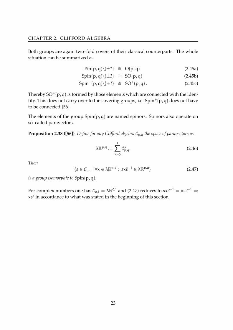
Both groups are again two–fold covers of their classical counterparts. The whole
situation can be summarized as
Pin(p, q)\±1 ∼= O(p, q) (2.45a)
Spin(p, q)\±1 ∼= SO(p, q) (2.45b)
Spin+(p, q)\±1 ∼= SO+(p, q) . (2.45c)
Thereby SO+(p, q) is formed by those elements which are connected with the iden-
tity. This does not carry over to the covering groups, i.e. Spin+(p, q) does not have
to be connected [56].
The elements of the group Spin(p, q) are named spinors. Spinors also operate on
so–called paravectors.
Proposition 2.38 ([56]) Define for any Clifford algebra Cp,q the space of paravectors as
λRp,q :=
1∑
k=0
Ckp,q. (2.46)
Then
s ∈ Cp,q | ∀x ∈ λRp,q : sxs−1 ∈ λRp,q (2.47)
is a group isomorphic to Spin(p, q).
For complex numbers one has C0,1 = λR0,1 and (2.47) reduces to sxs−1 = xss−1 =:
xs ′ in accordance to what was stated in the beginning of this section.
23

2.4 THE CLIFFORD GROUP
24

Chapter 3
Basic Clifford Neurons
Neurons are the atoms of neural computation. Out of those simple computational
units all neural networks are build up. An illustration of a generic neuron is given
in figure 3.1. The output computed by a generic neuron reads
y = g(f(w, x)) . (3.1)
f g
1x
y
xn
w
wn
1
Figure 3.1: Model of a generic neuron.
The details of computation are as follows. In a first step the input to the neuron,
x := xi, is associated with the weights of the neuron, w := wi, by invoking the
so–called propagation function f. This can be thought as computing the activation
potential from the pre–synaptic activities. Then from that result the so-called acti-
vation function g computes the output of the neuron. The weights, which mimic
synaptic strength, constitute the adjustable internal parameters of the neuron. The
process of adapting the weights is named learning. In accordance to the thesis
introduction only supervised learning will be considered here.
Supervised learning is often characterized as learning with a ”teacher”. This means
25

that full feedback on the performance is provided throughout the learning process
and learning itself is goal–driven. Technically, ”the teacher” is realized in the fol-
lowing way. A training set (xp, dp)Pp=1 consisting of correct input–output patterns
is provided. Performance is measured by evaluating some given error function E.
The most common error function is
E :=1
2P
P∑
p=1
‖ dp− yp ‖2 , (3.2)
which measures the derivation between desired and actual output in the mean–
squared sense. Learning is then formulated as finding the optimal weights that
minimize E on the given training set. The actual goal of learning, however, is gen-
eralization. That is to perform well on unseen data. Generalization performance is
therefore measured on a test set, which is disjoint from the training set. The accu-
rate partition of data into the two sets is a complex problem both theoretically [89]
and practically [92], especially when there is ”not enough” data available.
Searching the weight space is done iteratively. This is a consequence of the neural
computation paradigm itself. Which iterative technique is applicable depends on
the properties of the error function E. If all partial derivatives ∂E∂wi
exist error mini-
mization can be done by performing gradient descent. In that case the weights are
changed according to
w(t+ 1) = w(t) − η∂E
∂w. (3.3)
In the rule above η is a real positive constant controlling the steepness of the update
step. An update step is usually called an epoch. Using (3.3) requires a full scan
through the training set. An alternative to this batch learning is to update the
weights after each presented pattern p
w(t+ 1) = w(t) − η∂Ep
∂w, (3.4)
whereby the true gradient (3.2) is replaced by
Ep :=1
2‖ dp− yp ‖2 . (3.5)
Ep, which is only an approximation of E, is referred to as the stochastic gradient
and therefore the weight update (3.4) is also named stochastic. Another common
name for learning using (3.4) is online learning, which highlights the fact that no
internal storage of training patterns is required. Each of the two learning regimes
has its own advantages and disadvantages. Batch learning allows a deeper and
26

CHAPTER 3. BASIC CLIFFORD NEURONS
easier understanding of the dynamics of neurons and is therefore the appropriate
choice for most theoretical studies.
From the biological point of view it is advisable to use an integrative propagation
function. A therefore convenient choice would be to use the weighted sum of the
input
f(w, x) =∑
i
wixi , (3.6)
that is the activation potential equals the scalar product of input and weights
f(w, x) = 〈w, x〉 . (3.7)
In fact, (3.6) is the most popular propagation function since the dawn of neural
computation, however it is often used in the slightly different form
f(w, x) =∑
i
wixi+ θ . (3.8)
Obviously, setting w := (wi, θ) and x := (xi, 1) yields (3.7) again. The special
weight θ is called bias. Applying
Θ(x) =
1 : x > 0
0 : x ≤ 0(3.9)
as activation function to (3.8) yields the famous perceptron of Rosenblatt. In that
case θ works as a threshold. Besides (3.8) there are of course many other possi-
ble propagation functions. Another function of theoretical importance and some
broader practical use is
f(w, x) =∏
i
xwii , (3.10)
which aggregates the input signals in a multiplicative manner. A learning rule
for neurons based on (3.10) is given in [52]. Mostly, such neurons are studied in
boolean domains only. Summation as in (3.8) can be viewed as modelling linear
correlation of the inputs. In pattern recognition so-called higher–order neurons
y = g(w0+∑
i
wixi+∑
i,j
wi,jxixj+∑
i,j,k
wi,j,kxixjxk+ . . .) (3.11)
are known for a long time. Such neurons allow, to some extend, geometrically in-
variant learning of patterns. The drawback lies in the number of required weights,
which for a k–th order neuron with n inputs equals
k∑
i=0
(
n + i− 1
i
)
=
(
n+ k
k
)
. (3.12)
27

To overcome that exponential explosion of higher–order terms sigma–pi units were
proposed, in which only a certain small number of higher–order terms is used.
Unfortunately, that either requires to hard–wire appropriate terms in advance or
to restrict the order of neurons to a small number, say 2 or 3, in advance. Due to
such issues the practical use of higher–order neurons is limited, even in the field of
pattern recognition.
If (3.8) is supplemented with the identity as activation function and real–valued
domains are given a real linear neuron
y =∑
i
wixi+ θ (3.13)
is obtained. When used together with the error function (3.2) ordinary linear re-
gression is computed. The real linear neuron (3.13) can be seen as the first example
of a Clifford neuron. This is simply due to the isomorphism R ∼= C0,0,0 (section
2.2), which, in particular, also gives equivalence of real multiplication and geomet-
ric product in that case. Changing all underlying domains from real–valued to
Clifford–valued gives the generalization of (3.13) to neurons in arbitrary Clifford
algebras.
Definition 3.1 (Clifford Neuron) A Clifford Neuron (CN) computes the following func-
tion from (Cp,q,r)n to Cp,q,r
y =
n∑
i=1
wi⊗p,q,r xi+ θ . (3.14)
From the purely formal point of view Clifford neurons share with higher–order
neurons (3.11) the capability to process polynomial functions of the input. Also,
CNs could be formally interpreted as kind of a tensorial approach. However, these
are rather technical issues of little interest caused by top–level algebraic coherence.
The aim of this thesis is to demonstrate the usefulness of Clifford algebra for neural
computation due to its geometric nature. To actually start this challenge the special
case of a ”one–dimensional” Clifford Neuron shall be the first subject of detailed
study.
Definition 3.2 (Basic Clifford Neuron) A Basic Clifford Neuron (BCN) is derived from
a Clifford Neuron in the case of n = 1 in (3.14) and therefore computes the following func-
tion from Cp,q,r to Cp,q,ry = w⊗p,q,r x + θ . (3.15)
To denote a BCN of a particular algebra Cp,q,r the abbreviation BCNp,q,r will be used.
28

CHAPTER 3. BASIC CLIFFORD NEURONS
Clifford–valued error functions analog to (3.2) and (3.5) can be easily derived.
However, the simplified error function
Ep,q,r =1
2‖ d−w⊗p,q,r x + θ ‖2
=1
2‖ d− y ‖2
=1
2‖ error ‖2 (3.16)
is used in this chapter in order to reduce the notational complexity of update rules.
For the bias θ of a BCN a generic update rule can be formulated.
Proposition 3.3 For any BCNp,q,r the update rule for the bias θ reads
θ(t+ 1) = θ(t) + ∆θ
= θ(t) + error . (3.17)
Of course, Basic Clifford Neurons are only of interest for Clifford algebras of di-
mension greater than 1, in which case every quantity becomes a multi–dimensional
object itself. The real–valued ”counterpart” to which a BCN can be related is a
feed–forward neural network consisting of one layer of linear neurons. It is con-
venient to define such a network with linear neurons as in (3.7), that is without an
explicit bias weight. As mentioned before this is always possible without any loss
of generality.
Definition 3.4 (Linear Associator) A Linear Associator (LA) is a neural network con-
sisting of n inputs and m output neurons computing the following function from Rn to
Rm
y = Wx . (3.18)
Thereby the weight matrix W is of size m × n and an entry wij represents the weight
connecting the i–th input to the j–th output neuron.
The abbreviation LAn,m will be used to refer to a Linear Associator of a particular
size. An illustration of a LA3,2 is given below in figure 3.2. More material on the
Linear Associator is provided in appendix A.1.
Any Basic Clifford Neuron can be viewed as a certain LA. This is a simple conse-
quence of Theorem 2.17, which stated that any Clifford algebra is isomorphic to
some matrix algebra. Thus, using a BCN means to apply a certain algebraic model
to the data, namely that of the underlying Clifford algebra, instead of a general lin-
ear model when using a LA instead. In that sense a BCN is the most trivial example
29

3.1 THE 2D BASIC CLIFFORD NEURONS
W
y
x
Figure 3.2: Linear Associator LA3,2with 3 inputs and 2 output neurons.
for the model–based nature of the Clifford algebra approach to neural computa-
tion. Moreover, this algebraic model becomes also a geometric model whenever a
geometric interpretation for the general operation of the geometric product in use
is at hand.
Linear algebra can always be used in Clifford algebra if needed. This advantage
just carries over to Clifford neurons. In the next section the corresponding Basic
Clifford Neurons of the two–dimensional Clifford algebras (2D Basic Clifford Neu-
rons) are studied. This is the natural entry point for all Clifford neural computation.
It allows to become familiar with the topic. To elucidate the model-based nature of
the Clifford approach will be the main aim of the section. Also, the algorithmic ba-
sis for the later chapters on Clifford MLPs will be introduced there. Basic Clifford
Neurons are also the subject of section 3.2. However, the point of view is slightly
moved from neurons itself to inherent attributes of Clifford neural computation. In
particular, issues of data representation and isomorphisms will be discussed. Then
a section on Clifford Associators follows before the chapter will be concluded by a
summary of the obtained results.
3.1 The 2D Basic Clifford Neurons
The Basic Clifford Neuron (BCN), as introduced in (3.15), is the most simple possi-
ble Clifford neuron. The propagation function of a BCN is a certain linear transfor-
mation. Hence the BCN can be viewed as a model–based architecture (compared
to a generic Linear Associator). The Complex Basic Clifford Neuron, for exam-
ple, computes a scaling–rotation (Euclidean) followed by a translation (section 2.4).
Translation is a generic component common to all BCNs. Therefore the specific part
of the propagation function of a BCN is fully determined by the geometric prod-
30

CHAPTER 3. BASIC CLIFFORD NEURONS
uct of the underlying Clifford algebra. In this section all three 2D Basic Clifford
Neurons are studied from this point of view.
3.1.1 The Complex Basic Clifford Neuron
The geometric interpretation of the propagation function of the Complex Basic Clif-
ford Neuron (BCN0,1) was already reviewed at the beginning of this section. It is,
technically, based on the isomorphism of the circle group, formed by all complex
numbers of modulus one, and the group SO(2) (2.36). Hence, the transformation
group SO(2) can be identified as the computational core of the Complex BCN.
From (3.3) the following update rule
∆w0,1 = −∂E0,1
∂w= −
∂E01
∂w0e0−
∂E01
∂w1e1
= −((−y0+w0x0−w1x1)x0+ (−y1+w0x1+w1x0)x1) e0
−((+y0−w0x0+w1x1)x1+ (−y1+w0x1+w1x0)x0) e1
= (error0x0+ error1x1) e0+ (−error0x1+ error1x0) e1
= error⊗ 0,1 x . (3.19)
derives for the Complex Basic Clifford Neuron. The rule has a very simple form.
The error made by the neuron multiplied with the conjugate of the input yields the
amount of the update step.
For a CBCN with error function
ECBCN =1
2‖ d−w⊗ 0,1 x ‖2 (3.20)
the following result holds.
Proposition 3.5 The Hessian matrix of a Complex BCN with error function (3.20) is a
real matrix of the form
HCBCN =
(
a 0
0 a
)
. (3.21)
If the input is denoted by xp0 + x
p1e1
Pp=1 then
a =1
P
(
P∑
p=1
(xp0)2+
P∑
p=1
(xp1)2
)
. (3.22)
This can be concluded from Proposition A.1, which states the general linear case.
Since the matrix (3.21) has only one eigenvalue the following nice result is obtained.
31

3.1 THE 2D BASIC CLIFFORD NEURONS
Corollary 3.6 Batch learning for a Complex BCN with error function (3.20) converges in
only one step (to the global minimum of (3.20)) if the optimal learning rate (A.4) is used.
Proposition 3.5 says that a Complex BCN with error function (3.20) applies an in-
trinsic one–dimensional view to the data. That is the orientation parameterized by
the angle of rotation. In particular, this requires that the error function measures
the Euclidean distance.
For demonstration a little experiment was performed. A random distribution of
100 points (xp1, x
p2)100p=1 with zero mean, variance one and standard deviation one
was created as input set. Then this set of points was rotated about an angle of 63
degrees and scaled by a factor of 4.5 yielding the output set of the experiment. A
Complex BCN and a Linear Associator LA2,2were trained on that data using batch
learning with optimal learning rates according to (A.4). The observed learning
curves are reported in figure 3.3. Additionally, figure 3.4 shows the error surface of
the Complex BCN.
0 2 4 6 8 10 120
1
2
3
4
5
6
Epochs
MS
E
Linear AssociatorComplex BCN
7 8 9 10 11 120
0.2
0.4
0.6
0.8
1x 10⁻⁴
Epochs
MS
E
Linear AssociatorComplex BCN
Figure 3.3: Training errors of the Complex BCN and the Linear Associator
LA2,2. Learning curves over all epochs (left) and epochs 7 to 12 (right).
As stated by Corollary 3.6 the Complex BCN did indeed converge in one epoch. In
further steps of training Gaussian noise of different levels was added. Both archi-
tectures were then tested on the original noise–free data. The obtained results are
reported below in figure 3.5. The Linear Associator has more degrees of freedom
than the Complex BCN and no suitable model of the data. The performance of the
32

CHAPTER 3. BASIC CLIFFORD NEURONS
34
5
1
2
30
1
2
Figure 3.4: Error surface of the Complex BCN.
0.01 0.02 0.03 0.040
0.1
0.2
0.3
0.4
0.5
σ2
MS
E
LA (10 points)LA (100 points)CBCN (10 points)
Figure 3.5: Comparison of the test performance of the Complex BCN and the
Linear Associator LA2,2 as the MSE (measured on the original noise–free data)
versus the present Gaussian noise with variance σ2 during training.
−6 −4 −2 0 2 4 6−6
−4
−2
0
2
4
6
−6 −4 −2 0 2 4 6−6
−4
−2
0
2
4
6
Figure 3.6: Learned transformations by the Complex BCN (left) and the Linear
Associator LA2,2 (right) from noisy data (σ2 = 0.4). Points (learned output)
should lie on the grid junctions (expected output).
33

3.1 THE 2D BASIC CLIFFORD NEURONS
LA2,2 is clearly worse than that of the Complex BCN on a training set of only 10
points. Even if then trained on 100 points the LA2,2 performance is still worse than
that of the Complex BCN trained on only 10 points, which is also illustrated in
figure 3.6.
3.1.2 The Hyperbolic Basic Clifford Neuron
The computational properties of the Complex BCN were shown to be induced by
the group of unit complex numbers, or, equivalently, SO(2). This way a geomet-
ric interpretation for the propagation function of a Complex BCN could be easily
achieved.
The matrix representation of a unit hyperbolic number x = x0+ x1e1, which can be
derived from (2.30), reads [37]
x =
(
ǫ cosh(φ) ǫ sinh(φ)
ǫ sinh(φ) ǫ cosh(φ)
)
(3.23)
for some φ ∈ R and ǫ = ±1. Thus there are actually two types of unit hyperbolic
numbers. If |x0| > |x1| then ǫ = 1 in (3.23), and, if |x1| > |x0| then ǫ = −1 in (3.23)1.
Unit hyperbolic numbers form a group which is isomorphic to SO(1, 1). Moreover,
the numbers with ǫ = 1 in (3.23) form a subgroup being isomorphic to SO(1, 1)+.
Only the transformations belonging to SO(1, 1)+ are orientation preserving, and,
are therefore called hyperbolic rotations. The elements of SO(1, 1)\SO(1, 1)+ are
called anti–rotations. An illustration of the above is given in figure 3.7. Both type
of transformations form the computational core of the Hyperbolic BCN (BCN1,0).
−5 0 5−6
−4
−2
0
2
4
6
1 2
34
1’
2’
3’
4’
−5 0 5−6
−4
−2
0
2
4
6
1 2
34
1’
2’
3’
4’
Figure 3.7: Illustration of hyperbolic numbers acting as transformations in the
plane. Hyperbolic rotation about 30 degrees (left) and hyperbolic anti–rotation
about 30 degrees (right) of the unit square.
1|x0| = |x1| is not possible for a unit hyperbolic number.
34

CHAPTER 3. BASIC CLIFFORD NEURONS
The update rule for the Hyperbolic BCN is given by
∆w = −∂E1,0
∂w= −
∂E1,0
∂w0e0−
∂E1,0
∂w1e1
= −((−y0+w0x0+w1x1)x0+ (−y1+w0x1+w1x0)x1) e0
−((−y0+w0x0+w1x1)x1+ (−y1+w0x1+w1x0)x0) e1
= (error0x0+ error1x1) e0+ (error0x1+ error1x0) e1
= error⊗ 1,0 x . (3.24)
The product of the error made by the neuron with the input yields the amount of
the update step. Next, the dynamics of a Hyperbolic BCN with error function
EHBCN =1
2‖ d−w⊗ 1,0 x ‖2 (3.25)
are outlined.
Proposition 3.7 The Hessian matrix of a Hyperbolic BCN with error function (3.25) is a
real matrix of the form
HHBCN =
(
a b
b a
)
. (3.26)
If the input is denoted by xp0 + x
p1e1
Pp=1 then
a =1
P
(
P∑
p=1
(xp0)2+
P∑
p=1
(xp1)2
)
and b =2
P
P∑
p=1
xp0xp1 . (3.27)
The dynamics of a Hyperbolic BCN and a Linear Associator (on the same input set)
are related as follows.
Proposition 3.8 Assuming the same input set, batch learning, and the use of optimal
learning rates, a LA2,2 with standard error function ELA (A.1) will not converge faster
than a Hyperbolic BCN with error function (3.25).
This is a rather technical result from Proposition 3.7. Some more insights of the
dynamics for a Hyperbolic BCN can be gained by a little experiment, for which a
similar setup as in section 3.1.1 was chosen.
The input set was created from a random distribution of 100 points (xp1, x
p2)100p=1
with zero mean, variance one and standard deviation one. From that the output
set was created by applying the anti-rotation induced by the hyperbolic number
35

3.1 THE 2D BASIC CLIFFORD NEURONS
2 + 4e1. The learning curves for the Hyperbolic BCN and the LA2,2 are shown in
figure 3.8.
0 1 2 3 4 50
1
2
3
4
5
Epochs
MS
E
Linear AssociatorHyperbolic BCN
Figure 3.8: Training errors of the Hyperbolic BCN and the Linear Associator
LA2,2.
The Hyperbolic BCN converged faster than the Linear Associator. In figure 3.9
(left) the error surface of the Hyperbolic BCN is plotted. The contour lines are el-
lipses which are rotated about 45 degrees w.r.t. to the origin. Actually, this is a
consequence of Proposition 3.7, i.e. it holds for any Hyperbolic BCN. That is the
eigenvectors of the Hessian (3.26) are always predetermined. Unfortunately, this is
not the case for the ratio of its eigenvalues. Therefore no generic coordinate trans-
formation can be applied in advance. Since all of the above depends on the used
error function a more ”hyperbolic” error function seems tempting. Of course, the
hyperbolic norm is the first candidate to look at. The hyperbolic norm, however,
does not induce a metric on the whole R2, and, is therefore not applicable as can be
seen from figure 3.9 (right).
34
5
1
2
30
1
2
34
5
1
2
30
0.5
1
1.5
Figure 3.9: Error surface of the Hperbolic BCN as induced by the Euclidean
norm (left) and the hyperbolic norm (right).
36

CHAPTER 3. BASIC CLIFFORD NEURONS
As outlined above, the geometric model (based on the group SO(1, 1)) by which
a Hyperbolic BCN looks at the data is not intrinsically one–dimensional. How-
ever, its presence can be clearly observed from the results presented in figure 3.10.
The Hyperbolic BCN trained on 10 points outperformed the Linear Associator on
noisy data. Even if the LA was trained with 100 points. This can also be seen
from figure 3.11 which gives a visualization of the learned transformations for one
particular noise level.
0.01 0.02 0.03 0.040
0.05
0.1
0.15
0.2
0.25
0.3
0.35
σ2
MS
E
LA (10 points)LA (100 points)HBCN (10 points)
Figure 3.10: Comparison of the test performance of the Hyperbolic BCN and
the Linear Associator LA2,2 as the MSE (measured on the original noise–free
data) versus the present Gaussian noise with variance σ2 during training.
−6 −4 −2 0 2 4 6−6
−4
−2
0
2
4
6
−6 −4 −2 0 2 4 6−6
−4
−2
0
2
4
6
Figure 3.11: Learned transformations by the Hyperbolic BCN (left) and the
Linear Associator LA2,2 (right) from noisy data (σ2 = 0.4). Points (learned
output) should lie on the grid junctions (expected output).
37

3.1 THE 2D BASIC CLIFFORD NEURONS
3.1.3 The Dual Basic Clifford Neuron
The Dual Basic Clifford Neuron (BCN0,0,1) remains as the last object for exami-
nation. In contrast to the other two 2D Basic Clifford Neurons it is based on a
degenerate Clifford algebra. However, there is also a pretty easy interpretation of
dual numbers as transformations acting in the plane. Every dual number induces
a shear transformation having the y–axes as fixed–line (see figure 3.12 for an illus-
tration). This also gives a geometric derivation for the set of zero divisors of C0,0,1(2.28).
−5 0 5−6
−4
−2
0
2
4
6
1 2
34
1’
2’
3’
4’
Figure 3.12: Illustration of dual numbers acting as transformations in the
plane. The unit square transformed by the shearing transformation induced
by the dual number 4+ 1e1.
The degenerate nature of C0,0,1 also effects the update rule for the Dual BCN which
reads
∆w = −∂E0,0,1
∂w= −
∂E0,0,1
∂w0e0−
∂E0,0,1
∂w1e1
= −((−y0+w0x0)x0+ (−y1+w0x1+w1x0)x1) e0
−( 0 + (−y1+w0x1+w1x0)x0) e1
= (error0x0+ error1x1) e0+ (0+ error1x0) e1 . (3.28)
In contrast to the previous neurons the update rule can not be formulated in terms
of the underlying geometric product ⊗ 0,0,1. Also, no quantitative statement inde-
pendent of a particular data set can be made for the dynamics of a Dual BCN. The
Hessian of a Dual BCN can not be narrowed down to a particular form. Therefore,
the only thing that remains to check about a Dual BCN is the performance on noisy
data. For that purpose a little experiment was performed again.
As in the previous experiments of this section the input set consisted of 100 2D–
points drawn from a distribution having zero mean, variance one and standard
38

CHAPTER 3. BASIC CLIFFORD NEURONS
deviation one. For the output set those points were transformed by the shearing
induced by the dual number 2+ 4e1. The error surface of the Dual BCN computed
for the input set is shown in figure 3.13, which is of course a paraboloid.
34
5
1
2
30
1
2
Figure 3.13: Error surface of the Dual BCN.
For the given data the Linear Associator did converge faster than the Dual BCN as
can be seen from figure 3.14.
0 2 4 6 80
1
2
3
4
5
Epochs
MS
E
Linear AssociatorDual BCN
Figure 3.14: Training errors of the Dual BCN and the Linear Associator LA2,2.
However, for training in the presence of noise similar numerical results as in the
previous experiments were obtained. The Dual BCN, possessing the right model
for the data, outperformed the Linear Associator, which, without such a model, fol-
lowed much more the noise in the data. This becomes even more clear by looking
at the visualizations of the learned transformations provided in figure 3.16.
39

3.1 THE 2D BASIC CLIFFORD NEURONS
0.01 0.02 0.03 0.040
0.05
0.1
0.15
0.2
0.25
0.3
0.35
σ2
MS
E
LA (10 points)LA (100 points)DBCN (10 points)
Figure 3.15: Comparison of the test performance of the Dual BCN and the
Linear Associator LA2,2 as the MSE (measured on the original noise–free data)
versus the present Gaussian noise with variance σ2 during training.
From all the introduced 2D Basic Clifford neurons the Dual BCN implies internally
the strongest constraints to the fitted data. This makes it2 obviously weaker than
the other neurons in the following sense. Suppose we want to approximate a gen-
eral linear mapping. This seems intuitively easier by a superposition of scaling–
rotations, i.e. by an architecture based on Complex BCNs than by a superposition
of shearing transformation, i.e. by an architecture based on Dual BCNs. For the
case of Hyperbolic BCNs it is hard to come up with any such intuition.
−2 −1 0 1 2−6
−4
−2
0
2
4
6
−2 −1 0 1 2−6
−4
−2
0
2
4
6
Figure 3.16: Learned transformations by the Dual BCN (left) and the Linear
Associator LA2,2 (right) from noisy data (σ2 = 0.4). Points (learned output)
should lie on the grid junctions (expected output).
2More precisely, architectures based on it.
40

CHAPTER 3. BASIC CLIFFORD NEURONS
3.2 Isomorphic BCNs and Isomorphic Representations
For every natural numbern > 1 there exist Clifford algebras of dimension 2nwhich
are isomorphic to each other (see table 2.2). Basic Clifford Neurons (BCNs) are
solely determined by the geometric product of the underlying algebra. Therefore
it is quite natural to assume that isomorphic Clifford algebras also induce ”isomor-
phic” BCNs. Proving this assumption and determining its precise meaning is the
first goal of this section. The closely related topic of isomorphic representations is
then discussed afterwards.
3.2.1 Isomorphic Basic Clifford Neurons
Isomorphic Clifford algebras first occur in dimension four, namely C1,1 and C2,0 (see
table 2.2). Those two algebras will serve as an example throughout this section.
Their multiplication tables are given below in table 3.1 and table 3.2, respectively.
⊗ 1,1 1 e1 e2 e1e2
1 1 e1 e2 e1e2
e1 e1 1 e1e2 e2
e2 e2 −e1e2 −1 e1
e1e2 e1e2 −e2 −e1 1
Table 3.1: Multiplication table of the Clifford algebra C1,1.
⊗ 2,0 1 e1 e2 e1e2
1 1 e1 e2 e1e2
e1 e1 1 e1e2 e2
e2 e2 −e1e2 1 −e1
e1e2 e1e2 −e2 e1 −1
Table 3.2: Multiplication table of the Clifford algebra C2,0.
The multiplication tables do only slightly differ. Therefore the two algebras are
related by a rather simple isomorphism.
Proposition 3.9 The map φ : C1,1 → C2,0
x0+ x1e1+ x2e2+ x12e12 7→ x0+ x12e1+ x1e2− x2e12 (3.29)
41
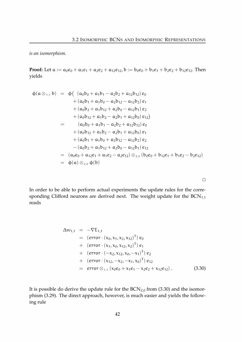
3.2 ISOMORPHIC BCNS AND ISOMORPHIC REPRESENTATIONS
is an isomorphism.
Proof: Let a := a0e0+ a1e1+ a2e2+ a12e12, b := b0e0+ b1e1+ b2e2+ b12e12. Then
yields
φ(a⊗ 1,1 b) = φ(
(a0b0+ a1b1− a2b2+ a12b12) e0
+ (a0b1+ a1b0− a2b12− a12b2) e1
+ (a0b2+ a1b12+ a2b0− a12b1) e2
+ (a0b12+ a1b2− a2b1+ a12b0) e12)
= (a0b0+ a1b1− a2b2+ a12b12) e0
+ (a0b12+ a1b2− a2b1+ a12b0) e1
+ (a0b1+ a1b0+ a2b12− a12b2) e2
− (a0b2+ a1b12+ a2b0− a12b1) e12
= (a0e0+ a12e1+ a1e2− a2e12) ⊗ 2,0 (b0e0+ b12e1+ b1e2− b2e12)
= φ(a) ⊗ 2,0 φ(b)
2
In order to be able to perform actual experiments the update rules for the corre-
sponding Clifford neurons are derived next. The weight update for the BCN1,1
reads
∆w1,1 = −∇E1,1
= (error · (x0, x1, x2, x12)T) e0
+ (error · (x1, x0, x12, x2)T) e1
+ (error · (−x2, x12, x0,−x1)T) e2
+ (error · (x12,−x2,−x1, x0)T) e12
= error⊗ 1,1 (x0e0+ x1e1− x2e2+ x12e12) . (3.30)
It is possible do derive the update rule for the BCN2,0 from (3.30) and the isomor-
phism (3.29). The direct approach, however, is much easier and yields the follow-
ing rule
42

CHAPTER 3. BASIC CLIFFORD NEURONS
∆w2,0 = −∇E2,0
= (error · (x0, x1, x2, x3)T) e0
+ (error · (x1, x0, x12, x2)T) e1
+ (error · (x2,−x12, x0,−x1)T) e2
+ (error · (−x12, x2,−x1, x0)T) e12
= error⊗ 2,0 (x0e0+ x1e1+ x2e2− x12e12) . (3.31)
To get an understanding of isomorphic Clifford neurons the following experiment
was performed with the neurons BCN1,1 and BCN2,0. As input set for the BCN1,1
four3 4–dimensional points were randomly drawn. Any input point (regarded as
a multivector in C1,1) was multiplied from the left with 1e0 + 2e1 + 3e2 + 4e12 via
the geometric product ⊗ 1,1. That way the BCN1,1 output set was created. Then the
isomorphism φ (3.29) was applied to both sets yielding the input and output data
for the BCN2,0. Both neurons were trained by batch learning with optimal learning
rate. The optimal learning rate for the two neurons turned out to be identical. The
initial multivector weights of the neurons were set according to table 3.3.
w(0) e0 e1 e2 e12
BCN1,1 +0.3462 +0.0252 -0.2974 +0.2721
BCN2,0 +0.3381 -0.4804 +0.1813 -0.1205
Table 3.3: Initial multivector weights for the BCN1,1 and the BCN2,0.
The obtained learning curves (see figure 3.17) only differ at the very first epochs of
training.
3That small number of points was chosen to exclude any kind of averaging effects.
43

3.2 ISOMORPHIC BCNS AND ISOMORPHIC REPRESENTATIONS
0 1 2 3 4 5 61
2
3
4
5
Epochs
MS
E
BCN1,1
BCN2,0
Figure 3.17: Training errors of the BCN1,1 and the BCN2,0.
Training was finished after 50 epochs and the neurons converged indeed to ”iso-
morphic” solutions as reported in table 3.4. In addition, isomorphic initial multi-
vector weights resulted in totally identical learning dynamics.
w(50) e0 e1 e2 e12
BCN1,1 +1.0000 +1.9999 +2.9994 +3.9999
BCN2,0 +1.0000 +3.9994 +1.9999 -2.9994
Table 3.4: Multivector weights for the BCN1,1 and the BCN2,0 after 50 epochs
of training. Equivalence of the results follows from the isomorphism (3.29).
A formal notion for identical dynamics of isomorphic Basic Clifford Neurons is
presented in the next theorem. The result holds for both online and batch learning.
Theorem 3.10 Let φ be an isomorphism from Cp,q to Cp′,q′ . Let BCNp,q be a neuron
trained on a training set (xp, dp)P
p=1 with learning rate η and initial multivector weight
w0p,q. Furthermore, letwtp,q denote the multivector weight of BCNp,q after t training steps.
Then the neuron BCNp′,q′ trained on the training set (φ(xp), φ(dp))P
p=1 with learning
rate η and initial multivector weight φ(w0p′,q′) has the multivector weight φ(wtp′,q′) after
t steps of training.
Besides being very powerful, the statement of Theorem 3.10 seems very intuitive
at first sight. However, it is only valid because every isomorphism of two Clifford
algebras is of particular simple nature (likewise (3.29)). This can be seen more
clearly from the following important corollary.
44

CHAPTER 3. BASIC CLIFFORD NEURONS
Corollary 3.11 Let the assumptions of Theorem 3.10 be valid. Then two neurons BCNp,qand BCNp′,q′ have the same optimal learning rate for batch learning.
This corollary, taken into account Proposition A.2, puts some restrictions on the
nature of the underlying algebra isomorphism. Therefore Theorem 3.10 results
from the very insights of Clifford algebra.
All of the above motivates the following definition.
Definition 3.12 The two neurons BCNp,q and BCNp′,q′ are called isomorphic if Cp,q ∼=
Cp′,q′ holds.
Anything that can be computed by a Basic Clifford Neuron can also be computed
with equivalent dynamics (Theorem 3.10) by any other isomorphic BCN. In that
sense, two isomorphic Basic Clifford Neurons are identical neural architectures.
Then, so being all Clifford neural architectures that only differ by isomorphic neu-
rons.
3.2.2 Isomorphic Representations
There are many fundamental differences between Clifford neural networks and
standard real–valued ones. Many of them are related to how the data is seen by
them, or, how the data can be represented to them. In what follows the technical
basis for data representation inside the Clifford framework is outlined. Many pow-
erful applications of this feature of Clifford neural computation will be given later
in this thesis.
For a fully–connected real–valued neural network neither the order of the compo-
nents of a presented input vector nor the order of the components of a presented
output vector has a semantical meaning. Consider for example the Linear Asso-
ciator LA4,4 trained on a training set (xp1, x
p2, x
p3, x
p4), (d
p1, d
p2, d
p3, d
p4)Pp=1. Present-
ing the training set (xp4, x
p1, x
p2, x
p3), (d
p4, d
p1, d
p2, d
p3)Pp=1 is obviously the same task.
Therefore both data representations can be viewed as ”isomorphic” for a LA4,4.
Nothing new or different is gained by using the second one instead of the first one.
This is very similar to the notion of isomorphic neurons we have discussed before.
However, the same data representations as above
(x1e0+ x2e1+ x3e2+ x4e12)p, (d1e0+ d2e1+ d3e2+ d4e12)
pPp=1 (3.32)
45

3.2 ISOMORPHIC BCNS AND ISOMORPHIC REPRESENTATIONS
and
(x4e0+ x1e1+ x2e2+ x3e12)p, (d4e0+ d1e1+ d3e2+ d3e12)
pPp=1 (3.33)
are not isomorphic for the BCN1,1. The order of components is relevant for Clifford
neurons. Multivectors are, for Clifford neurons, tuples, and, a geometrical semantic
is induced by the graded subspace structure of the underlying Clifford algebra. In
order to proceed the next rather technical definition is needed.
Definition 3.13 (Isomorphic Representations for Basic Clifford Neurons) Two rep-
resentations f : R2p+q+r
→ Cp,q,r and g : R2p+q+r
→ Cp′,q′,r′ are called (left–)isomorphic if
for all x ∈ R2p+q+r
and for all y ∈ Cp,q,r there exists some y ′ ∈ Cp′,q′,r′ such that
f(x) ⊗p,q,r y = g(x) ⊗p ′,q ′,r ′ y′ . (3.34)
Obviously the algebras have to be of same dimension for (3.34) to hold. Isomorphic
representations define equivalence classes of data representations. For example,
one might be interested in isomorphic representations to (3.32) for the BCN1,1. This
translates to Cp,q,r = Cp′,q′,r′ = C1,1,0 , f = id and then asking for permutations g
fulfilling (3.34).
Of course, the most interesting thing about isomorphic representations are the un-
derlying data representations itself. The most important class of representations
for Clifford neural computation arises from presenting lower–dimensional data to
higher–dimensional Clifford neurons. This may be the normal case since every
Clifford algebra is particularly of dimension 2n. Moreover, representing data in
such a way may often be intended, since it allows for many uses of the subspace
grading of a Clifford algebra. Then it is much more precise to speak of lower–
dimensional objects (having a semantical meaning, say vectors, for example) that
are presented. The next chapter will introduce a new Clifford neuron solely de-
signed for that purpose.
Knowledge of isomorphic representations for the above type of representations is
therefore essential. However, in its general form the problem of determining all
possible isomorphic presentations cannot be treated efficiently. This is simply due
to the following combinatorial argument. It is a common fact that the number of
combinations of n things taken k at a time is(
n
k
)
=n!
k!(n − k)!. (3.35)
There are(
n
k
)2possibilities for representing a k–dimensional data set to a Basic Clif-
ford Neuron of dimension n. For example, 3–dimensional data can be presented to
46

CHAPTER 3. BASIC CLIFFORD NEURONS
a 8–dimensional BCN, say BCN1,1,1, in 3136 ways. Plugging k = 4 and n = 16 into
(3.35) yields 3312400 possibilities.
Let us consider the following two–dimensional data representations
(1) : (x1e0+ x2e1+ 0e2+ 0e12)p, (d1e0+ d2e1+ 0e2+ 0e12)
p
(2) : (x1e0+ 0e1+ x2e2+ 0e12)p, (d1e0+ 0e1+ d2e2+ 0e12)
p
(3) : (x1e0+ 0e1+ 0e2+ x2e12)p, (d1e0+ 0e1+ 0e2+ d2e12)
p
(4) : (0e0+ x1e1+ x2e2+ 0e12)p, (0e0+ d1e1+ d2e2+ 0e12)
p
(5) : (0e0+ x1e1+ 0e2+ x2e12)p, (0e0+ d1e1+ 0e2+ d2e12)
p
(6) : (0e0+ 0e1+ x1e2+ x2e12)p, (0e0+ 0e1+ d1e2+ d2e12)
p .
for the BCN1,1 as a walk–trough example.
Proposition 3.14 The following relations hold
BCN1,1(1) ∼= BCN1,1(6) (3.36)
BCN1,1(2) ∼= BCN1,1(5) (3.37)
BCN1,1(3) ∼= BCN1,1(4) . (3.38)
Proof: Statement (3.36) is verified by the following little computation
(x1e0+ x2e1+ 0e2+ 0e12) ⊗1,1 (ae0+ be1+ ce2+ de12)
= (x1a+ x2b)e0+ (x1b+ x2a)e1+ (x1c+ x2d)e2+ (x1d + x2c)e12
= (0e0+ 0e1+ x1e2+ x2e12) ⊗1,1 (ce0− de1− ae2+ be12)
The other results follow by similar simple computations. 2
Note that
(x1e0+ x2e2) ⊗1,1 (ae0+ be2) = (x1− a)e0+ (x2+ b)e2 (3.39)
and
(x1e1+ x2e2) ⊗1,1 (ae1+ be2) = (x1+ a)e1+ (x2+ b)e2 . (3.40)
Thus (3.39) is the multiplication of complex numbers and (3.40) is the multiplica-
tion of hyperbolic numbers. Both types are therefore encoded in the BCN1,1.
In the remainder of this section we will now deal with representations of affine
transformations of the plane. This is a useful class of propagation functions and a
nice way to summarize all the topics of this section in one example.
47

3.2 ISOMORPHIC BCNS AND ISOMORPHIC REPRESENTATIONS
3.2.3 Example: Affine Transformations of the Plane
An affine transformation of the plane is a mapping from R2 to R2 of the form
(x, y)T 7→(
a b
c d
)
(x, y)T +
(
tx
ty
)
. (3.41)
In Clifford algebra such transformation can be expressed in either of the two iso-
morphic algebras C1,1 and C2,0. The algebra C2,0 will be treated first. The direct
approach of using the vector representation x1e1 + x2e2, however, does not work.
Suitable representations can be found by utilizing the fact R(2) ∼= C2,0 (table 2.2).
Proposition 3.15 The map
R(2) → C2,0,
(
a b
c d
)
7→1
2((a+ d)e0+ (a− d)e1+ (b+ c)e2+ (b− c)e12) (3.42)
is an isomorphism.
The application of the transformation matrix in (3.41) can also be written in the
slightly more complicated way
(
a b
c d
)
(x, y)T =
(
a b
c d
)(
x 0
y 0
)
. (3.43)
Transforming
(
x 0
y 0
)
by (3.42) yields 12(xe0+xe1+ye2−ye12), which allows the
following statement4.
Proposition 3.16 For any real data (xp1, x
p2), (d
p1, d
p2)Pp=1 the BCN2,0 trained on the train-
ing set (x1e0+x1e1+x2e2−x2e12)p, (d1e0+d1e1+d2e2−d2e12)
pPp=1 converges to the
best affine approximation of the data (assuming the use of an appropriate learning rate).
Note that nothing inside the neuron has to be changed. Applying the isomorphism
(3.42) to the multivector weight w of the trained neuron gives the transformation
matrix of (3.41). Similarly, applying (3.42) to the multivector bias θ yields the trans-
lation vector of (3.41).
From the definition of an affine transformation (3.41) and with the methods out-
lined above the following result is easily obtained.
4The factor 12
can be neglected.
48

CHAPTER 3. BASIC CLIFFORD NEURONS
Proposition 3.17 The representations
(x1e0+ x1e1+ x2e2− x2e12)p, (d1e0+ d1e1+ d2e2− d2e12)
pPp=1 (3.44)
and
(x2e0+ x2e1+ x1e2− x1e12)p, (d2e0+ d2e1+ d1e2− d1e12)
pPp=1 (3.45)
are the only isomorphic representations for a BCN2,0 representing affine transformations
(in the sense of Proposition 3.16).
The existence of suitable presentations of affine transformations for the BCN1,1 is
guaranteed by Theorem 3.10, and, all such presentation can be directly derived by
applying the inverse isomorphism of (3.29) to (3.44) and (3.45).
Proposition 3.18 The representations
(x1e0+ x2e1+ x2e2+ x1e12)p, (d1e0+ d2e1+ d2e2+ d1e12)
pPp=1 (3.46)
and
(x2e0+ x1e1+ x1e2+ x2e12)p, (d2e0+ d1e1+ d1e2+ d2e12)
pPp=1 (3.47)
are the only isomorphic representations for a BCN1,1 representing affine transformations
(in the sense of Proposition 3.16).
Of course, the same representations derive from the following isomorphism from
R(2) to C1,1.
Proposition 3.19 The map
R(2) → C1,1,
(
a b
c d
)
7→1
2((a+ d)e0+ (b+ c)e1+ (c− b)e2+ (a− d)e12) (3.48)
is an isomorphism.
Applying (3.48) to
(
x 0
y 0
)
and
(
y 0
x 0
)
yields (3.46) and (3.47), respectively.
A lot of new technical terms for Clifford neural computation were introduced in
this section. Most important, we saw how Basic Clifford Neurons incorporate dif-
ferent propagation functions, which are ”selectable” from the outside by applying
different representations.
49

3.3 THE CLIFFORD ASSOCIATOR
3.3 The Clifford Associator
So far we have been studying only single Basic Clifford Neurons. Technically, a
Basic Clifford Neuron (Definition 3.2) was introduced as one–dimensional special
case of a Clifford Neuron (Definition 3.1). The latter will be used now to introduce
the first Clifford neural network of this thesis.
Definition 3.20 (Clifford Associator) A Clifford Associator (CA) is a Clifford neural
network consisting of n inputs and m output Clifford Neurons computing the following
function from (Cp,q,r)n to (Cp,q,r)
m
y = W ⊗ x , (3.49)
with x and y both being tuples of multivectors and W being a weight matrix of sizem× n
having multivector entries. An entrywij represents the multivector weight connecting the
i–th input to the j–th output Clifford Neuron. The weight matrixW is applied to the input
x by means of the tensor product ⊗.
The above definition is only heavy–weighted with respect to the amount of needed
formalism. A Clifford Associator is the natural generalization of a Linear Associa-
tor as introduced in Definition 3.4. In particular, the latter is obtained by plugging
C0,0,0 into Definition 3.20. From the pure technical point of view the Clifford Asso-
ciator can also be seen as a tensor network [63].
Obviously, isomorphic Clifford algebras give isomorphic Clifford Associators. The
number of real parameters of a Clifford Associator of size m× n is given by
NCAm,n = m · n · 2p+q+r . (3.50)
The update rule for the multivector weightwij of a Clifford Associator with under-
lying algebra Cp,q,r is the same as for the Basic Clifford Neuron BCNp,q,r having xi,
yj and dj as its input, actual computed output and expected output, respectively.
In this section only one particular Clifford Associator will be studied. This will be
the Dual Clifford Associator of size 3× 3 (shortly referred to as DCA3,3). This spe-
cific architecture is chosen in order to highlight another feature of Clifford neural
computation. It offers the possibility to directly process other geometric entities
besides points. In the following an example for the processing of lines is worked
out.
There are many ways to represent lines [68]. A very old one are Plucker coordinates
[66].
50

CHAPTER 3. BASIC CLIFFORD NEURONS
Definition 3.21 (Plucker Coordinates) Let l be a line in Euclidean 3D space repre-
sented by a point p = p1, p2, p3 lying on l and the direction vector q = q1, q2, q3
of l. Let q′ := p× q be the moment vector. Then the six element vector
L := (q, q′) (3.51)
gives the so–called Plucker coordinates of l.
The following connection between Plucker coordinates and dual numbers trace
back to Clifford himself [19].
Proposition 3.22 Let L1 = (q11, q12, q13, q11′, q12′, q13′), L2 = (q21, q22, q23, q21′, q22′,
q23′) be Plucker coordinates of two lines related by an Euclidean transformation. Then
there exists a 3× 3 dual number matrix W such that
q21+ q21′e1q22+ q22′e1q23+ q23′e1
= W
q11+ q11′e1q12+ q12′e1q13+ q13′e1
. (3.52)
The explicit matrix representation of the 3D Euclidean group E(3) in terms of dual
number matrices is given, for example, in [78]. A detailed discussion about the
advantages of (3.52) over the common representation of E(3) by homogenous coor-
dinates and 4× 4 matrices for robotics can be found in [71].
Transformations of lines under E(3) can be learned by a Dual Clifford Associator
DCA3,3 if the lines are presented in accordance to Proposition 3.22. This is also
possible by a Linear Associator LA6,6. Note that the DCA3,3 has 18 real parameters
and the LA6,6 has 36 real parameters (3.50). Both architectures were compared in
the following experimental setup.
05
10
0
5
100
2
4
6
Figure 3.18: Training set for the Clifford Associator DCA3,3 and the Linear
Associator LA6,6 consisting of 6 lines.
51

3.3 THE CLIFFORD ASSOCIATOR
The input set consisted of the 6 lines shown in figure 3.18. A rotation about the axis
(2, 2, 3) and through 30 degrees followed by a translation by (1, 2, 3) was chosen as
learning task. Using batch learning with optimal learning rate the Linear Associa-
tor needed around 12000 epochs to reach a training error (MSE) less than 0.01. The
same error level was reached by the DCA3,3 in about 100 epochs. A comparison
of the two learning curves as provided by figure 3.19 also shows, that the DCA3,3came up with a very good approach already after the first epoch. For the DCA3,3the same learning rate as for the LA6,6 was used.
0 20 40 60 80 1000
5
10
15
20
25
30
35
Epochs
MS
E
Linear AssociatorDual Clifford Associator
Figure 3.19: Training errors of the Dual Clifford Associator DCA3,3 and the
Linear Associator LA6,6.
The Dual Clifford Associator also outperformed the Linear Associator in terms of
generalization. Both networks were trained on data corrupted by Gaussian noise
of different levels and then tested on the original noise–free data. The obtained
results averaged over 20 runs are reported in figure 3.20. Not surprisingly, the
Linear Associator basically learned the noise and only weak generalization did
happen. In contrast, the Dual Clifford Associator was able to still generalize well
even for higher levels of noise. This can be concluded from the fact that the MSE on
the test set was always below the MSE on the training set, which has the following
simple explanation. The DCA3,3 computes the best fitting dual–number matrix W
(3.52), and therefore representing the data in terms of Plucker coordinates (lines)
forces a constraint optimization. Applying the same data to the LA6,6, however,
has noch such effect.
52

CHAPTER 3. BASIC CLIFFORD NEURONS
0.01 0.02 0.03 0.040
0.05
0.1
0.15
0.2
0.25
σ2
MS
E
Linear AssociatorDual Clifford Associator
0.01 0.02 0.03 0.040
0.2
0.4
0.6
0.8
1
1.2
1.4
σ2
MS
E
Linear AssociatorDual Clifford Associator
Figure 3.20: Performance of the Dual Clifford Associator DCA3,3 and the Lin-
ear Associator LA6,6 when trained on data with added Gaussian noise with
variance σ2. The left plot shows training performance and the right plot shows
test performance (also in correspondence to the level of noise on the training
set) on the original noise–free data.
The above experiment showed that, even if it is always theoretical possible to use a
Linear Associator instead of a Clifford Associator, it may be totally unpractical for a
particular task. Also, there is no generic way to present lines in an only real–valued
architecture. However, this is exactly the sort of prior knowledge one might wish to
communicate to a neural architecture. For example, many algorithms in computer
vision are line based and deliver results in terms of lines (e.g. edge detection).
One Clifford neural architecture can handle different geometric entities, or, more
precisely, this feature is encoded via the geometric product inside the propagation
function. The Dual Clifford Associator as introduced above can handle points as
well. Everything only depends on the way the data is represented.
3.4 Summary of Chapter 3
In this chapter we undertook the first steps into the theory of Clifford neural com-
putation. As its atom the Basic Clifford Neuron (BCN) was introduced. The com-
putation of a BCN is solely determined by one geometric product associating one
multivector weight with the received input. Particulary, the BCNs corresponding
to the three two–dimensional Clifford algebras have been studied in great detail.
Those neurons were compared in several experiments to the Linear Associator in
order to highlight the model–based nature of Clifford neural computation. Theo-
retically, this was demonstrated by deriving the different optimal learning rates for
those neurons (Proposition 3.7, Corollary 3.8, and Proposition 3.10) based on the
53

3.4 SUMMARY OF CHAPTER 3
classical work of LeCun [51] for the Linear Associator. The standard error func-
tions (SSE/MSE) were shown to be also the appropriate choice for the Clifford
framework. From the particular nature of the derived update rule (3.28) for the
Dual BCN the influence of the underlying degenerate Clifford algebra could be
made visible.
The new theoretical concepts of isomorphic Basic Clifford Neurons and isomorphic
representations have been presented. The first allows to identify equivalent neural
Clifford architectures. This was proven theoretically and shown experimentally for
the isomorphic neurons BCN1,1 and BCN2,0. Equivalence was shown to be hold up
to the level of learning dynamics (Theorem 3.10) and (Corollary 3.11). Any Clifford
neuron applies to the data it sees a certain geometric model induced by the under-
lying Clifford algebra. That fact allows a rich variety of data representations which
then can be classified by the concept of isomorphic representations. As an example
different representations for affine transformations have been studied. With both
mentioned concepts the core set of tools for the systematic study of Clifford neural
computation has been laid.
Finally, the Linear Associator was generalized to the Clifford Associator. The Dual
Clifford Associator based on the algebra C0,0,1was compared with the Linear Asso-
ciator on data represented by lines. In an experiment that illustrates the capability
of a Clifford architecture to intrinsical process lines, the Dual Clifford Associator
outperformed the Linear Associator, with respect to both the number of needed
training epochs and generalization capability.
54

Chapter 4
Spinor Clifford Neurons
In the previous chapter we utilized Clifford algebra to introduce neurons allow-
ing for the computation of transformations of different geometric entities. Both the
type of entities to process and the transformations to compute could be commu-
nicated to the neuron just by presenting the data in a certain specific way. Thus,
although everything remained on a numerical level, structural a priori knowledge
could be integrated. The study of this key feature of Clifford neural computation
continues in this chapter. A second type of Clifford neuron is introduced, which
has the following motivation.
The step from 2D Basic Clifford Neurons to Basic Clifford Neurons of higher di-
mensions yields only generalization in algebraical terms. What is still missing is
generalization in terms of geometry. The propagation function of a Complex Basic
Clifford Neuron, for example, is representing a 2D Euclidean transformation plus
scaling, or, equivalently, the action of the corresponding transformation group on
points in the plane. No Basic Clifford Neuron has a 3D Euclidean transformation
as propagation function. This is due to the in general two–sided operation of the
Clifford group (section 2.4), which prompts for the following new type of Clifford
neuron.
Definition 4.1 (Spinor Clifford Neuron) For any p+ q > 1 a Spinor Clifford Neuron
(SCN) computes the following function from Cp,q to Cp,q
y = w⊗p,q x⊗p,q φ(w) + θ , (4.1)
with φ being either inversion ˜, reversion ^, or conjugation ¯, respectively. For a particular
Spinor Clifford Neuron the acronym SCNφp,q is used.
A Spinor Clifford Neuron, basically, mimics the action of the Clifford group. There-
55

fore a SCN is only defined for non–degenerate Clifford algebras. Also, the propa-
gation function (4.1) is only useful for non–commutative algebras, hence the con-
dition p+ q > 1. A SCN is a neural architecture based on two geometric products.
However, its multivector weights, coupled by the involution φ, are not indepen-
dent. Therefore a Spinor Clifford Neuron has actually only one independent mul-
tivector weight. Consequently, a SCN has the same number of free parameters as
a BCN of same dimension. It is of course possible to study Clifford neurons with
two uncoupled weights
y = w1⊗p,q x⊗p,q w2+ θ . (4.2)
Here we will only consider SCNs due to their distinctive geometric properties,
which do not apply for the more general neurons of the form (4.2).
To every Spinor Clifford Neuron the standard error function
Esp,q =1
2‖ d −w⊗p,q x⊗p,q φ(w) + θ ‖2
=1
2‖ d − y ‖2
=1
2‖ error ‖2 (4.3)
is associated. The bias term in (4.1) is common to all SCNs. The generic bias up-
date rule for the Basic Clifford Neuron (3.3) does also apply in case of a SCN. The
dynamics of the BCN and the SCN, however, differ as follows.
Proposition 4.2 Let HBCNp,q be the Hessian of a Basic Clifford Neuron BCNp,q. Then
HSCN
φp,q
= 2HBCNp,q (4.4)
is the Hessian of the Spinor Clifford Neuron SCNφp,q.
This gives immediately the following result.
Corollary 4.3 Let ηopt be the optimal learning rate for a Basic Clifford NeuronBCNp,q.Then12ηopt is the optimal learning rate for the Spinor Clifford Neuron SCNφp,q.
Both statements above are very intuitive because a SCN is linear and based on two
geometric products.
The following discussion of Spinor Clifford Neurons follows the same structure
used in chapter three for Basic Clifford Neurons. First, we will study the most
56

CHAPTER 4. SPINOR CLIFFORD NEURONS
simple representative of a Spinor Clifford Neuron. That way all relevant aspects of
Spinor Clifford Neurons can be introduced in an illustrative manner. Afterwards,
the topic of isomorphic SCNs and isomorphic representations is studied in detail.
The last section of this chapter presents a method for linearizing the computation
of Mobius transformations by a single SCN using a conformal data representation.
4.1 The Quaternionic Spinor Clifford Neuron
The most simple Spinor Clifford Neurons are those of dimension four. Among
them the SCN derived from the algebra of quaternions C0,2 is of particular interest
and importance.
Definition 4.4 (Quaternionic Spinor Clifford Neuron) The Quaternionic Spinor Clif-
ford Neuron (Quaternionic SCN) computes the following function from C0,2 to C0,2
y = w⊗ 0,2 x⊗ 0,2 w+ θ . (4.5)
The Quaternionic SCN is also the most exceptional Spinor neuron since it has the
following unique properties. First, it can be used in the following canonical way
(in accordance to the given motivation of SCNs). For any vector x1e1 + x2e2 the
Quaternionic SCN computes a 2D orthogonal transformation followed by a trans-
lation. If the multivector weightw of a Quaternionic SCN is a unit quaternion then
the propagation function is a 4D Euclidean transformation [27, 56]. If in the latter
case a multivector x1e1+ x2e2+ x12e12 is presented a 3D Euclidean transformation
results. Taken into account that quaternions are nowadays established as a fast way
for computing 3D rotations the last presented fact is of most practical relevance.
Surprisingly, only ordinary quaternionic multiplication was considered as propa-
gation function by Arena et al. [1] when proposing their Quaternionic MLP. Net-
works based on (4.5) will be introduced later in chapter five. At the moment we
are only interested in the Quaternionic Spinor Clifford Neuron itself, for which the
following update rule can be derived
57
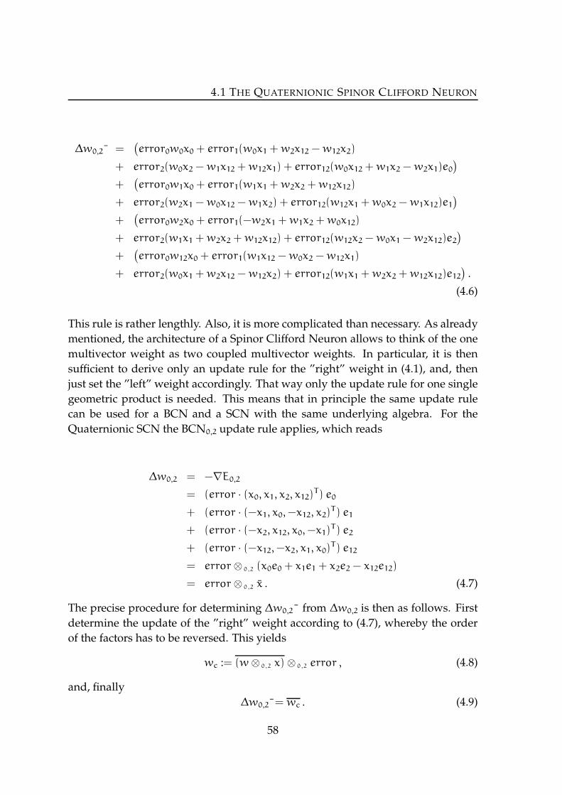
4.1 THE QUATERNIONIC SPINOR CLIFFORD NEURON
∆w0,2¯ =(
error0w0x0+ error1(w0x1+w2x12−w12x2)
+ error2(w0x2−w1x12+w12x1) + error12(w0x12+w1x2−w2x1)e0)
+(
error0w1x0+ error1(w1x1+w2x2+w12x12)
+ error2(w2x1−w0x12−w1x2) + error12(w12x1+w0x2−w1x12)e1)
+(
error0w2x0+ error1(−w2x1+w1x2+w0x12)
+ error2(w1x1+w2x2+w12x12) + error12(w12x2−w0x1−w2x12)e2)
+(
error0w12x0+ error1(w1x12−w0x2−w12x1)
+ error2(w0x1+w2x12−w12x2) + error12(w1x1+w2x2+w12x12)e12)
.
(4.6)
This rule is rather lengthly. Also, it is more complicated than necessary. As already
mentioned, the architecture of a Spinor Clifford Neuron allows to think of the one
multivector weight as two coupled multivector weights. In particular, it is then
sufficient to derive only an update rule for the ”right” weight in (4.1), and, then
just set the ”left” weight accordingly. That way only the update rule for one single
geometric product is needed. This means that in principle the same update rule
can be used for a BCN and a SCN with the same underlying algebra. For the
Quaternionic SCN the BCN0,2 update rule applies, which reads
∆w0,2 = −∇E0,2
= (error · (x0, x1, x2, x12)T) e0
+ (error · (−x1, x0,−x12, x2)T) e1
+ (error · (−x2, x12, x0,−x1)T) e2
+ (error · (−x12,−x2, x1, x0)T) e12
= error⊗ 0,2 (x0e0+ x1e1+ x2e2− x12e12)
= error⊗ 0,2 x . (4.7)
The precise procedure for determining ∆w0,2¯ from ∆w0,2 is then as follows. First
determine the update of the ”right” weight according to (4.7), whereby the order
of the factors has to be reversed. This yields
wc := (w⊗ 0,2 x) ⊗ 0,2 error , (4.8)
and, finally
∆w0,2¯= wc . (4.9)
58

CHAPTER 4. SPINOR CLIFFORD NEURONS
In order to demonstrate the equivalence of the two update methods (4.6) and (4.7)
the following experiment was performed using online learning1. A random distri-
bution of 100 4D points (xp1, x
p2, x
p3, x
p4)100p=1 with zero mean, variance one and stan-
dard deviation one was created. Interpreted as quaternions, this set of points was
conjugated by a unit quaternion corresponding to a rotation about the axis (2, 2, 3)
and through 30 degrees and finally translated about (0, 2, 2,−1). On that created
training set several runs of a Quaternionic SCN with the two different update meth-
ods (4.6) and (4.7) were performed using a fixed initial multivector weight and a
fixed learning rate η = 0.2. All runs converged to the solution in the same number
of iterations. Differences of the learning curves could only be observed by explicitly
studying absolute deviation between runs. Two examples are reported in figure 4.1
below. As can be seen from that plot the deviation for runs with different update
methods was in the same range as that in between runs using (4.6). Thus both up-
date methods are indeed equivalent. The observed differences between the runs
were caused by using training data with precision of 15 digits, which means that
training took place close to machine precision.
0 20 40 60 800
0.2
0.4
0.6
0.8
1x 10⁻³
Iterations
Dev
iatio
n (a
bsol
ute)
Setting ISetting II
Figure 4.1: Absolute difference of training errors between two runs of the
Quaternionic Spinor Clifford Neuron. In one case (referred to as setting I) up-
date rule (4.6) was used for both runs, in the other case (referred to as setting II)
update rules (4.6) and (4.7) were used in the first and second run, respectively.
In a second experiment only the last three components of the above training data
sets were used. Thus the learning task was changed to be a 3D Euclidean transfor-
mation. On that task the Quaternionic SCN was compared with a Linear Associator
LA4,4 for which the bias term was incorporated as described in chapter three. On-
line learning was used with a learning rate η = 0.2 for the LA4,4 and a learning rate
1Remember that in the regime of online learning a weight update is performed after every single
presentation of a pattern, which is referred to as one iteration of the training.
59

4.1 THE QUATERNIONIC SPINOR CLIFFORD NEURON
η = 0.1 for the Quaternionic SCN, respectively. The resulting learning curves are
presented in figure 4.2.
0 20 40 60 800
0.5
1
1.5
2
2.5
3
3.5
Epochs
MS
E
Linear AssociatorQuaternionic SCN
Figure 4.2: Training errors of the Quaternionic SCN and the Linear Associator
LA4,4.
Although oscillating at the beginning of training the Quaternionic SCN converged
faster than the LA4,4. After 50 training patterns the Quaternionic SCN has reached
an error below 10−5, for which the LA4,4 needed about 70 patterns. Numerical re-
sults for noisy data are reported below in figure 4.3. The results are pretty similar to
all the ones obtained in previous experiments. The Quaternionic SCN outperforms
the general linear architecture in terms of generalization from noisy data. Clearly,
this is due to the Quaternionic SCN possesses the right model for the data.
0.01 0.02 0.03 0.040.3
0.4
0.5
0.6
0.7
0.8
0.9
1
σ2
MS
E
Linear AssociatorQuaternionic SCN
0.01 0.02 0.03 0.040.2
0.4
0.6
0.8
1
1.2
1.4
1.6
σ2
MS
E
Linear AssociatorQuaternionic SCN
Figure 4.3: Performance of the Quaternionic SCN and the Linear Associa-
tor LA4,4 when trained on data with added Gaussian noise with variance σ2.
The left plot shows training performance and the right plot shows test per-
formance (in correspondence to the level of noise on the training set) on the
original noise–free data.
60

CHAPTER 4. SPINOR CLIFFORD NEURONS
The amount of outperforming, however, becomes really impressive when looking
at the transformed test data itself, which consisted of the vertices of the 3D object
already known from section 3.3, figure 3.18. The position and orientation of the
object is not well recovered by the LA4,4 (see figure 4.4 (right)), whereas the task
was still managed satisfactory by the Quaternionic SCN.
Figure 4.4: Learned transformations by the Quaternionic SCN (left) and the
Linear Associator LA4,4 (right) from noisy data (σ2 = 0.03). Points (learned
output) should lie on the vertices of the shaded object (expected output).
The main result of this section, however, is that the update rule for a SCN can be
expressed very efficiently by using that of the BCN with same underlying algebra.
4.2 Isomorphic Spinor Clifford Neurons
One of the main results of chapter three was that Clifford neural architectures
which only differ by isomorphic Basic Clifford Neurons are identical. Spinor Clif-
ford Neurons, however, are not based on Basic Clifford Neurons. This would only
be true for neurons of the form (4.2) with two independent weights. A Spinor
Clifford Neuron, however, has two dependent weights which are coupled by an
involution as introduced in Definition 4.1. This makes the SCN a Clifford neuron
of its own rights. Therefore, the question of isomorphic Spinor Clifford Neurons is
not covered by the aforementioned framework.
Since Spinor Clifford Neurons are determined by both a particular geometric prod-
uct and a particular involution it is helpful to have an explicit notion of the latter.
The involutions occurring for SCNs of dimension four and eight are given below
in table 4.1 and table 4.2, respectively.
61

4.2 ISOMORPHIC SPINOR CLIFFORD NEURONS
e0 e1 e2 e12
Reversion (^) + + + -
Inversion (˜) + - - +
Conjugation (¯) + - - -
Table 4.1: Involutions for Clifford algebras of dimension four.
e0 e1 e2 e3 e12 e13 e23 e123
Reversion (^) + + + + - - - -
Inversion (˜) + - - - + + + -
Conjugation (¯) + - - - - - - +
Table 4.2: Involutions for Clifford algebras of dimension eight.
For every Clifford algebra of dimension greater than two the occurring involutions
are distinct from each other. This easily prompts the following statement.
Proposition 4.5 Let SCNφp,q and SCNψp,q be two isomorphic Spinor Clifford Neurons.
Then φ = ψ.
Thereby, two SCNs are regarded as being isomorphic in the same sense as be-
fore (section 3.2). Particularly, Theorem (3.10) holds analogously. The statement
of Proposition 4.5 can be further generalized as follows.
Proposition 4.6 Let SCNφp,q and SCNψp′,q′ be two isomorphic Spinor Clifford Neurons.
Then φ = ψ and Cp,q ∼= Cp′,q′ .
Thus, two SCNs can only be isomorphic if the underlying Clifford algebras are
isomorphic too. For example, SCN ¯2,0 is not isomorphic to the Quaternionic SCN.
Otherwise, C2,0 would be isomorphic to the Clifford algebra of quaternions C0,2.
Underlying isomorphic Clifford algebras are necessary but not sufficient for two
SCNs to be isomorphic. This can be seen from the example of the SCN ˜1,1 and the
SCN ˜2,0. To be able to actually perform computations the following two isomor-
phisms from the underlying Clifford algebras of these neurons to R(2) are needed
first.
62

CHAPTER 4. SPINOR CLIFFORD NEURONS
Proposition 4.7 The map ψ11
C1,1 → R(2), x0e0+ x1e1+ x2e2+ x12e12 7→(
x0+ x12 x1− x2
x1+ x2 x0− x12
)
(4.10)
is an isomorphism.
Proposition 4.8 The map ψ20
C2,0 → R(2), x0e0+ x1e1+ x2e2+ x12e12 7→(
x0+ x1 x2+ x12
x2− x12 x0− x1
)
(4.11)
is an isomorphism.
Let φ11 denote the isomorphism from R(2) to C1,1 (3.42) and φ20 denote the isomor-
phism from R(2) to C2,0 (3.48), respectively.
Furthermore, setW :=
(
3 4
−7 8
)
and X :=
(
2 12
3 −5
)
. Then
ψ11(
(φ11(W) ⊗ 1,1 φ11(X)) ⊗ 1,1 φ11(W)˜)
=
(
32 120
−460 −1062
)
,
whereas
ψ20(
(φ20(W) ⊗ 2,0 φ20(X)) ⊗ 2,0 φ20(W)˜)
=
(
118 2
−466 −1032
)
.
Therefore, the two Spinor Clifford Neurons SCN ˜1,1 and SCN ˜
2,0 are not isomorphic.
The same values forW and X as above can be used to show that SCN^1,1 and SCN^
2,0
are also not isomorphic. Contrary to that the following result holds.
Proposition 4.9 The neurons SCN ¯1,1 and SCN ¯
2,0 are isomorphic.
Proof: Let w11 := w0e0+w1e1+w2e2+w12e12 be the weight of the SCN ¯1,1. Then
ψ11(w11) =
(
w0−w12 −w1+w2
w1−w2 w0+w12
)
=: W11 .
Furthermore, w20 := w0e0 + w12e1 + w1e2 − w2e12 is the image of w11 under the
algebra isomorphism (3.29) from C1,1 to C2,0. Now direct computation shows
ψ20(w20) = ψ20(w0e0−w12e1−w1e2+w2e12)
=
(
w0−w12 −w1+w2
w1−w2 w0+w12
)
= W11 .
63

4.2 ISOMORPHIC SPINOR CLIFFORD NEURONS
2
All of the above can be summarized as follows.
Theorem 4.10 The only 4–dimensional isomorphic Spinor Clifford Neurons are SCN ¯1,1
and SCN ¯2,0.
The fact that C1,2 ∼= C(2) ∼= C3,0 can be utilized to derive a similar theorem for the
eight–dimensional case, for which the easy proof by direct computation will be
omitted here.
Theorem 4.11 The only 8–dimensional isomorphic Spinor Clifford Neurons are SCN ¯1,2
and SCN ¯3,0.
Since explicitly designed for modelling the operation of the Clifford group, the
standard data for Spinor Clifford Neurons are vectors. Therefore, for example,
(4) : (0e0+ x1e1+ x2e2+ 0e12)p, (0e0+ d1e1+ d2e2+ 0e12)
p
is the corresponding vector representation of four–dimensional Spinor Clifford
Neurons. From the isomorphism of the Clifford groups
Γ0,2∼= Γ2,0 (4.12)
follows immediately
SCN ¯2,0(4)
∼= SCN ¯0,2(4) . (4.13)
Note that in contrast BCN0,2 6∼= BCN2,0 as well as SCN0,2 6∼= SCN2,0. Hence (4.12)
only induces isomorphic vector representations. Moreover, the vector representa-
tion is well distinguished from other possible representations, for example, those
given by
(1) : (x1e0+ x2e1+ 0e2+ 0e12)p, (d1e0+ d2e1+ 0e2+ 0e12)
p
(2) : (x1e0+ 0e1+ x2e2+ 0e12)p, (d1e0+ 0e1+ d2e2+ 0e12)
p
(3) : (x1e0+ 0e1+ 0e2+ x2e12)p, (d1e0+ 0e1+ 0e2+ d2e12)
p
(5) : (0e0+ x1e1+ 0e2+ x2e12)p, (0e0+ d1e1+ 0e2+ d2e12)
p
(6) : (0e0+ 0e1+ x1e2+ x2e12)p, (0e0+ 0e1+ d1e2+ d2e12)
p .
Proposition 4.12 The vector representation SCN ¯2,0(4) is unique in the following sense
SCN ¯2,0(4) 6
∼= SCN ¯0,2(i) (4.14)
for all i ∈ (1), (2), (3), (5), (6).
64

CHAPTER 4. SPINOR CLIFFORD NEURONS
Proof: The scalar component of
(w0e0+w1e1+w2e2+w12e12)⊗ 2,0 (x1e1+ x2e2)⊗ 2,0 (w0e0−w1e1−w2e2−w12e12)
is zero where as it is nonzero for the spinor multiplications corresponding to the
representations (1),(2),(3),(5) and (6). 2
The above generalizes in that sense that there are much less isomorphic representa-
tions for Spinor Clifford Neurons than for Basic Clifford Neurons. When proceed-
ing to Clifford neural networks later in this thesis we will concentrate on vector
representations. For Euclidean transformations as propagation functions it is suffi-
cient to study only Spinor Clifford Neurons based on conjugation. An application
of a SCN based on reversion is given in the subsequent section.
4.3 Linearizing Mobius Transformations
Spinor Clifford Neurons allow the computation of general orthogonal transforma-
tions. For that purpose many different linear representations can be chosen as
demonstrated before. A very interesting application of a nonlinear representation
will be studied in the following. By using a so–called conformal representation2 a
Spinor Clifford Neuron based on reversion can compute a Mobius transformation
in a linear way.
Definition 4.13 ( Mobius Transformation) For every a, b, c, d ∈ C with ad−bc 6= 0
the mapping
C → C, z 7→az+ b
cz+ d(4.15)
is called a Mobius transformation.
Mobius transformations are a specific class of holomorphic functions. They are of
great importance in many mathematical branches. For example, they belong to the
heart of monogenic functional calculus [45]. Moreover, Mobius transformations
form the isometries of the Poincare model (unit disk) of the hyperbolic plane. Ev-
ery Mobius transformation is a conformal mapping, that is, it preserves angles.
Hence there is a close relation to orthogonal mappings. More precisely, the Mobius
transformations (4.15) form a group M isomorphic to O(1, 2)/±1 (see e.g. [67]).
2In terms of Geometric Algebra this concept is referred to as the conformal model of the Eu-
clidean Geometric Algebra (CGA) [40].
65
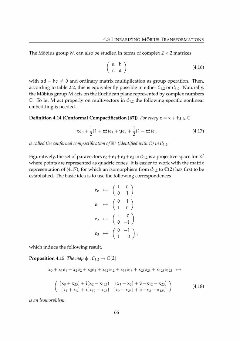
4.3 LINEARIZING MOBIUS TRANSFORMATIONS
The Mobius group M can also be studied in terms of complex 2× 2 matrices
(
a b
c d
)
(4.16)
with ad − bc 6= 0 and ordinary matrix multiplication as group operation. Then,
according to table 2.2, this is equivalently possible in either C1,2 or C3,0. Naturally,
the Mobius groupM acts on the Euclidean plane represented by complex numbers
C. To let M act properly on multivectors in C1,2 the following specific nonlinear
embedding is needed.
Definition 4.14 (Conformal Compactification [67]) For every z = x + iy ∈ C
xe0+1
2(1+ zz)e1+ ye2+
1
2(1− zz)e3 (4.17)
is called the conformal compactification of R2 (identified with C) in C1,2.
Figuratively, the set of paravectors e0+e1+e2+e3 in C1,2 is a projective space for R2
where points are represented as quadric cones. It is easier to work with the matrix
representation of (4.17), for which an isomorphism from C1,2 to C(2) has first to be
established. The basic idea is to use the following correspondences
e0 7→(
1 0
0 1
)
e1 7→(
0 1
1 0
)
e2 7→(
i 0
0 −i
)
e3 7→(
0 −1
1 0
)
,
which induce the following result.
Proposition 4.15 The map φ : C1,2 → C(2)
x0+ x1e1+ x2e2+ x3e3+ x12e12+ x13e13+ x23e23+ x123e123 7→
(
(x0+ x23) + i(x2− x123) (x1− x3) + i(−x12− x23)
(x1+ x3) + i(x12− x23) (x0− x23) + i(−x2− x123)
)
(4.18)
is an isomorphism.
66

CHAPTER 4. SPINOR CLIFFORD NEURONS
The image of the conformal compactification (4.17) of a point z under the above
isomorphism φ reads
(
z zz
1 z
)
. (4.19)
The following linearization of Mobius transformations in terms of the Clifford al-
gebra C1,2 is then easily verified by direct computation (see e.g. [67]).
Proposition 4.16 Let A =
(
a b
c d
)
be a complex matrix with ad − bc 6= 0. Let z be
the conformal compactification of a point (x, y) ∈ R2 according to (4.17). This yields
Aφ(z) A = λ
(
z ′ z ′z ′
1 z ′
)
, (4.20)
with 1λz ′ being the conformal compactification of the image of (x, y) under the Mobius
transformation induced by A and λ = ‖cz+ d‖2.
The general result for Rnwas proven by Vahlen [87] more than hundred years ago.
However, results on 2 × 2 Clifford matrices inducing Mobius transformations for
arbitrary quadratic spaces Rp,q became known not before around the 1990s (see e.g.
[20]).
The realization of Mobius transformations by the Spinor Clifford Neuron SCN ˜1,2 is
not so straightforward due to the existence of the real factor λ in (4.20). Of course, λ
can always be integrated as activation function. This, however, renders the whole
Clifford algebra approach more complicated than a direct implementation of (4.15).
It is also possible to scale in preprocessing either the input or the output by λ.
The drawback of that method is that it requires knowledge of the transformation
parameters in advance. This can be overcome by performing the scaling inside the
neuron. More precisely, the first component and the third component of the current
weight w can be used to compute λ [12], by which the original input x is divided
in a first step. If x ′ denotes such a scaled term the computation w ⊗ 1,2 x′ ⊗ 1,2 w
then follows. Therefore only the weight update for the last geometric product has
actually to be computed. This can be done by using the update rule
67

4.3 LINEARIZING MOBIUS TRANSFORMATIONS
∆w1,2 = −∇E1,2
= (error · (x0, x1, x2, x3, x12, x13, x23, x123)T) e0
+ (error · (x1, x0, x12, x13, x2, x3, x123, x23)T) e1
+ (error · (−x2, x12, x0,−x23,−x1, x123, x3,−x13)T) e2
+ (error · (−x3, x13, x23, x0,−x123,−x1,−x2, x12)T) e3
+ (error · (x12,−x2,−x1, x123, x0,−x23,−x13, x3)T) e12
+ (error · (x13,−x3,−x123,−x1, x23, x0, x12,−x2)T) e13
+ (error · (−x23,−x123,−x3, x2,−x13, x12, x0, x1)T) e23
+ (error · (−x123,−x23,−x13, x12,−x3, x2, x1, x0)T) e123
= error⊗ 1,2 (x0e0+ x1e1− x2e2− x3e3+ x12e12+ x13e13− x23e23− x123e123) .
(4.21)
and then compute the dependent weight in a similar way as demonstrated for the
Quaternionic SCN before (section 4.1).
For testing the above procedure the Mobius transformation
z 7→0.5(1+ i)z+ 0.5(1− i)
−0.5(1+ i)z+ 0.5(1− i)(4.22)
was chosen as learning task. The input set consisted of 100 data points (xp1, xp2)100p=1
from a distribution having zero mean, variance one and standard deviation one.
From those points the output set was created by applying transformation (4.22).
For both sets the conformal compactification (4.17) was then computed resulting in
the final sets for training. For stable convergence of batch learning a rather small
learning rate η = 0.001 was necessary. The learning curve of the SCN ˜1,2 is pre-
sented in figure 4.5.
0 200 400 600 800 10000
1
2
3
4
Epochs
MS
E
Figure 4.5: Training error of the SCN ˜1,2.
68

CHAPTER 4. SPINOR CLIFFORD NEURONS
Although a lot more epochs were needed, compared to the typical numbers re-
ported in the experiments on BCNs and SCNs we have done so far, learning suc-
ceeded with zero training error. Thus the exact parameters of the transformation
were learned by the SCN ˜1,2. This demonstrates the indented capability of the neu-
ron to perform Mobius transformations in a linear way when data is provided ac-
cording to (4.17).
Another such application of the SCN ˜1,2 arises from the well–known relation be-
tween Mobius transformations and the cross–ratio of an ordered quadruple of
points.
The cross–ratio of 4 points z, q, r, s ∈ R2 (identified with complex numbers) is given
by [60]
[z, q, r, s] =(z− q)(r− s)
(z− s)(r− q). (4.23)
It is a well known projective invariant from which many others can be derived [90].
The precise relation to Mobius transformations is given by the next theorem.
Theorem 4.17 ([60]) The cross–ratio [z, q, r, s] is the image of z under that Mobius trans-
formation that maps q to 0, r to 1 and s to ∞, respectively.
The task now for the SCN ˜1,2 was to learn to compute the cross–ratio(s) [z, q, r, s]
with q := 0.2+ i 0.3, r := 0.4− i 0.7, and s := 0.6− i 0.2. That is after being trained
on the set (q, 0), (r, 1), (s,∞)3 the neuron should be able to compute the cross–
ratio [z, q, r, s] when presented the test point z. Training was performed in batch
mode with learning rate set to η = 10−7. Due to the necessarily approximative
coding of ∞ the task could not be learned exactly. Therefore training was stopped
after the SSE dropped below 0.00001. This was the case after approximately 30000
epochs. A comparison between theoretical and learned transformation parameters
is given in table 4.3.
Parameter Theoretical value Learned value
a +0.20+ i 0.50 +0.20019 + i 0.50010
b +0.11- i 0.16 +0.11001 - i 0.15992
c -0.20+ i 1.00 -0.20079 + i 0.99939
d -0.08- i 0.64 -0.07930 - i 0.64007
Table 4.3: Comparison between theoretical and learned transformation pa-
rameters.
3The entity ∞ was coded as 1015.
69

4.4 SUMMARY OF CHAPTER 4
The difference between the actual values and those learned by the neuron is quite
small. Therefore an excellent performance on test points could be achieved as can
be seen from table 4.4.
Test point Theoretical value SCN ˜1,2 output value
2.0+i 3.0 +0.3578-i 0.3357 + 0.3577-i 0.3364
4.0-i 7.0 +0.4838-i 0.3044 + 0.4838-i 0.3051
0.3+i 0.1 +0.0077-i 0.6884 + 0.0082-i 0.6884
Table 4.4: Comparison between theoretical cross–ratio values (rounded) and
actual output cross–ratio values of the SCN ˜1,2 for some test points.
4.4 Summary of Chapter 4
In this chapter we introduced the class of Spinor Clifford Neurons (SCN). This sec-
ond fundamental type of Clifford neuron generalizes the two–dimensional Basic
Clifford Neurons in a geometrical sense. The computation of a Spinor Clifford
Neuron is an orthogonal transformation achieved by mimicking the two–sided op-
eration of the Clifford group. Although therefore technically involving two Clif-
ford products, a SCN has only one independent multivector weight. Thus a BCN
and a SCN of same dimension have the same number of free parameters. A result
relating the optimal learning rates of both types of Clifford neurons was presented
(Corollary 4.3). A general method for reducing the complexity of the update rule
for a SCN to that of BCN was derived. All of the above was demonstrated both
theoretically and by experiments for the Quaternionic SCN. This particular neuron
was also used to illustrate the general model–based nature of SCNs.
The question of isomorphic Spinor Clifford Neurons and isomorphic represen-
tations was studied. Necessary conditions for isomorphic SCNs were derived
(Proposition 4.7), and the two neurons SCN ¯1,1 and SCN ¯
2,0 were proven to be iso-
morphic. The so–called conformal representation was shown to enable a Spinor
Clifford Neuron to compute Mobius transformations in a linear way. This unique
property of the Clifford framework was utilized for neural computing of the cross–
ratio.
70
Chapter 5
Clifford MLPs with Real–Valued
Activation Functions
At the very beginning of chapter 3 we introduced y = g(f(w; x)) as the expression
for a generic neuron. In that setting the Basic Clifford Neuron (BCN) reads (see
Definition 3.2)
y = id(w⊗p,q,r x + θ) , (5.1)
and the Spinor Clifford Neuron (SCN) (see Definition 4.1) reads
y = id(w⊗p,q x⊗p,q φ(w) + θ) . (5.2)
The Linear Associator, which was introduced in Definition 3.4, consists of one fully
connected layer of real BCNs and, therefore, computes a linear mapping from Rn
to Rm
y = Wx , (5.3)
with weight matrix W := (wi,j)m,n. Adding another layer U is not beneficial since
y = U(Wx) would be of the same (linear) computational power as (5.3). If, how-
ever, a nonlinear activation function g in the first layer is used everything changes
dramatically. For understanding the new neural architecture derived in that way
y = U(∑
i
g(wijxj)) (5.4)
it is totally sufficient to restrict (5.4) to the case of one–dimensional output (because
only one type of activation function is used). Then the weight matrix U reduces to
a weight vector u yielding the simpler expression
y = ui(∑
i
g(wijxj)) . (5.5)
71

Asking for the functional power of that expression is a purely mathematical prob-
lem, which is stated outside the actual neural framework. One possible mathe-
matical view on (5.5) is that of a series with basis functions parameterised by the
individual weights wij.
Suppose now we want to actually train the architecture (5.5) by gradient descent.
For that purpose the nonlinear activation function g has to be bounded and dif-
ferentiable everywhere as well. All this is fulfilled by the class of the so–called
sigmoidal (”s–shaped”) functions.
Definition 5.1 (Sigmoidal Function) For everyβ 6= 0 the function σβ : R → R defined
by
x 7→1
1+ exp(−βx)(5.6)
is called a sigmoidal function.
Of course, the ”s–shaped” nature of sigmoidal functions is preserved under scaling
and translation. The functions 2σ2− 1 = tanh and σ1 are plotted in figure 5.1 . The
function σ1 is known as the logistic function.
−5 0 5−1
−0.5
0
0.5
1
−5 0 5−1
−0.5
0
0.5
1
Figure 5.1: Plot of the tanh function (left) and the logistic function (right).
The (re)–discovery1 of gradient descent for neural networks of type (5.4) with sig-
moidal activation functions by Rumelhart et al. [57] gave rebirth to the whole area
of neural computation and it meant nothing less than a revolution for the whole
field of artificial intelligence. Since that time training such a network by gradient
descent is known as Backpropagation and the network itself is famous as Multi-
layer Perceptron2 (MLP). The number of published papers on MLPs have become
1See [36] for more historical details.2Unfortunately, that name is quite misleading since the individual neurons are not Perceptrons.
72

CHAPTER 5. CMLPS WITH REAL–VALUED ACTIVATION
”uncountable” with respect to both the range of applications (image processing,
pattern recognition, speech recognition et cetera) and of research.
Soon after the publication of the Backpropagation algorithm the mathematical ca-
pabilities of MLPs have also been studied. A MLP with only one hidden layer
of sigmoidal functions was proven to be a universal approximator for the class of
continuous functions [23], which means that, theoretically, any such function can
be learned arbitrarily well. Even more important for the fast growing popularity of
the MLP was its ability to generalise well from training, which has been reported
for many different tasks (see e.g. [9, 25, 69]). A comprehensive treatment of gener-
alisation by MLPs can be found in [89].
From the formal point of view the MLP according to (5.4) can be easily generalised
to a Clifford architecture by just replacing the real BCN0,0,0 with BCNs or SCNs
of higher dimension. That is the activation function remains unchanged in the
following sense. The same real–valued activation function g is applied to every
component of the multivector argument. This yields (using the same notations
as in Proposition 2.24) the following expression for the multivector output of a
Clifford neuron (based on a BCN) in the first layer
∑
I∈I
g((w⊗p,q,r x+ θ)I)eI . (5.7)
A further step of generalisation could be the use of a Clifford–valued activation
function. For example, the complex logistic function
z 7→1
1+ exp(z)(5.8)
could be used as complex–valued activation function. Clifford Multilayer Percep-
trons with Clifford–valued activation functions are studied in the subsequent chap-
ter. In this chapter we will deal exclusively with the case of Clifford MLPs with
real–valued activation functions. The straightforward definition of such a Clifford
neural network is given below.
Definition 5.2 (Clifford MLP with Real–Valued Activation Functions) A Clifford
MLP with real–valued activation functions (CMLP) computes a function from (Cp,q,r)n
to (Cp,q,r)m by passing the input through a set 1, · · · , L of fully connected consecutive
layers. The output of the j-th neuron in the l-th layer reads
∑
I∈I
g(l)(∑
k
(w(l)
kj ⊗p,q,r x(l−1)
k + θ(l)
j )I)eI . (5.9)
73

5.1 BACKPROPAGATION ALGORITHM
Thereby x(l−1)
k denotes the k-th input from the previous layer (x(0)
k referring to the input of
the network itself) and g(l) denotes the real–valued activation function used for all neurons
in the l-th layer.
Using SCNs instead of BCNs gives a Spinor Clifford MLP.
Definition 5.3 (Spinor Clifford MLP with Real–Valued Activation Functions) A
Spinor Clifford MLP with real–valued activation functions (SCMLP) computes a function
from (Cp,q)n to (Cp,q)m by passing the input through a set 1, · · · , L of fully connected
consecutive layers. The output of the j-th neuron in the l-th layer reads
∑
I∈I
g(l)(∑
k
(w(l)
kj ⊗p,q x(l−1)
k ⊗p,q φ(wkj)(l) + θ
(l)
j )I)eI , (5.10)
and φ refers to one of the three possible involutions (conjugation, reversion, and inversion).
The last layer of a (S)CMLP is called the output layer, all other layers are called
hidden ones3. The neurons of a (S)CMLP are also called nodes. Mostly, we will
deal with two–layer (S)CMLPs. Two–layer CMLPs will be abbreviated as MLPg1,g2p,q,r
and two–layer SCMLPs which are based on conjugation will be abbreviated as
SMLPg1,g2p,q , respectively. In both cases gi stands for the function in the i–th layer.
If no functions are given g1 = σ1 and g2 = id is assumed. The only parameter
controlling the complexity of a two–layer (S)CMLP is the number of hidden nodes,
h. The total number of real parameters of such a network equals (set r = 0 for a
SCMLP)
N(S)CMLP = 2p+q+r · h · (n + 1) + 2p+q+r ·m · (h+ 1) . (5.11)
The chapter now proceeds as follows. The first section deals with the derivation
of the Backpropagation algorithm for (S)CMLPs, followed by discussing univer-
sal approximation in the second one. In the last section experimental results are
reported.
5.1 Backpropagation Algorithm
Training a Multilayer Perceptron using Backpropagation basically means to per-
form steepest gradient descent on a given error function with respect to the weights.
Thereby the errors are propagated backwards through the network, thus the name
3Remember that we do not count the network input as layer.
74
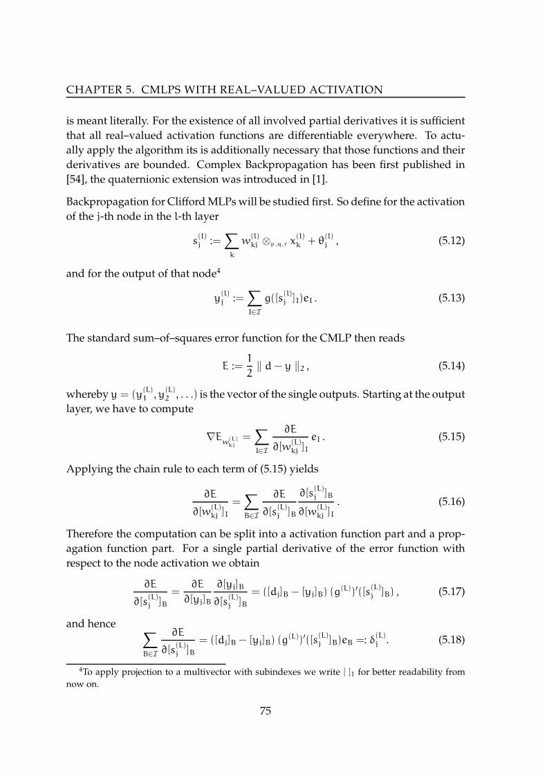
CHAPTER 5. CMLPS WITH REAL–VALUED ACTIVATION
is meant literally. For the existence of all involved partial derivatives it is sufficient
that all real–valued activation functions are differentiable everywhere. To actu-
ally apply the algorithm its is additionally necessary that those functions and their
derivatives are bounded. Complex Backpropagation has been first published in
[54], the quaternionic extension was introduced in [1].
Backpropagation for Clifford MLPs will be studied first. So define for the activation
of the j-th node in the l-th layer
s(l)
j :=∑
k
w(l)
kj ⊗p,q,r x(l)
k + θ(l)
j , (5.12)
and for the output of that node4
y(l)
j :=∑
I∈I
g([s(l)
j ]I)eI . (5.13)
The standard sum–of–squares error function for the CMLP then reads
E :=1
2‖ d − y ‖2 , (5.14)
whereby y = (y(L)
1 , y(L)
2 , . . .) is the vector of the single outputs. Starting at the output
layer, we have to compute
∇Ew
(L)
kj
=∑
I∈I
∂E
∂[w(L)
kj ]IeI . (5.15)
Applying the chain rule to each term of (5.15) yields
∂E
∂[w(L)
kj ]I=
∑
B∈I
∂E
∂[s(L)
j ]B
∂[s(L)
j ]B
∂[w(L)
kj ]I. (5.16)
Therefore the computation can be split into a activation function part and a prop-
agation function part. For a single partial derivative of the error function with
respect to the node activation we obtain
∂E
∂[s(L)
j ]B=
∂E
∂[yj]B
∂[yj]B
∂[s(L)
j ]B= ([dj]B− [yj]B) (g(L))′([s
(L)
j ]B) , (5.17)
and hence ∑
B∈I
∂E
∂[s(L)
j ]B= ([dj]B− [yj]B) (g(L))′([s
(L)
j ]B)eB =: δ(L)
j . (5.18)
4To apply projection to a multivector with subindexes we write [ ]I for better readability from
now on.
75

5.1 BACKPROPAGATION ALGORITHM
For many Clifford algebras we already know the remaining propagation function
term∂[s
(L)
j]B
∂[w(L)
kj ]Ifrom chapter 3 and thus (5.16) completely. For those algebras the up-
date rules for the weights of the output layer of the corresponding Clifford MLPs
are then as follows
C1,0,0 : ∆w(L)
kj =(3.24)
δ(L)
j ⊗1,0,0 y(L−1)
k (5.19)
C0,1,0 : ∆w(L)
kj =(3.19)
δ(L)
j ⊗0,1,0 y(L−1)
k (5.20)
C0,0,1 : ∆w(L)
kj =(3.28)
([δ(L)
j ]0[y(L−1)
k ]0+ [δ(L)
j ]1[y(L−1)
k ]1)e0+
([δ(L)
j ]1[y(L−1)
k ]0)e1 (5.21)
C0,2,0 : ∆w(L)
kj =(4.7)
δ(L)
j ⊗0,2,0 y(L−1)
k (5.22)
C1,1,0 : ∆w(L)
kj =(3.30)
δ(L)
j ⊗1,1,0 (y(L−1)
0 e0+ y(L−1)
1 e1− y(L−1)
2 e2+ y(L−1)
12 e12) (5.23)
C2,0,0 : ∆w(L)
kj =(3.31)
δ(L)
j ⊗2,0,0 (y(L−1)
0 e0+ y(L−1)
1 e1+ y(L−1)
2 e2− y(L−1)
12 e12) .(5.24)
For updating the weights in a hidden layer l we have to compute analogously to
(5.15)
∇Ew
(l)
kj
=∑
I∈I
∂E
∂[w(l)
kj ]IeI , (5.25)
yielding now
∂E
∂[w(l)
kj ]I=
∑
B∈I
∂E
∂[s(l)
j ]B
∂[s(l)
j ]B
∂[w(l)
kj ]I. (5.26)
Comparing (5.26) with (5.16) we see that the only5 remaining task is the compu-
tation of the new error terms ∂E
∂[s(h)
j ]B, which now involves the error terms from the
(h+1)-th layer. This results in slightly more complicated expressions. For example,
for the Clifford MLP with underlying degenerate Clifford algebra C0,0,1 the hidden
layer error terms read
δ(l)
j :=∑
B∈I
∂E
∂[s(l)
j ]B=
∂E
∂[s(l)
j ]0+
∂E
∂[s(l)
j ]1, (5.27a)
with
∂E
∂[s(l)
j ]0=
(
(
∑
m
[w(l)
jm]0[δ(l+1)m ]0
)(
(g(l))′([s(l)
j ]m))
+(
∑
m
[w(l)
jm]1[δ(l+1)m ]1
)(
(g(l))′([s(l)
j ]m))
)
e0 (5.27b)
5This is because all neurons have the same propagation function regardless of the layer.
76

CHAPTER 5. CMLPS WITH REAL–VALUED ACTIVATION
and∂E
∂[s(l)
j ]1=(
(
∑
m
[w(l)
jm]0[δ(l+1)m ]1
)(
(g(l))′([s(l)
j ]m))
)
e1) . (5.27c)
Finally, putting together (5.21) and (5.27a), the whole Backpropagation algorithm
for the MLP0,0,1 then reads
∆w(l)
kj = ([δ(l)
j ]0[y(l−1)
k ]0+ [δ(l)
j ]1[y(l−1)
k ]1)e0+ ([δ(l)
j ]1[y(l−1)
k ]0)e1 (5.28a)
∆θ(l)
j = δ(l)
j , (5.28b)
with δ(l)
j as in (5.18) if l = L, and δ(l)
j as in (5.27a) otherwise. The simple update
rule (5.28b) for the bias terms comes from the fact that such nodes can be viewed
as having constant input 1. Hence (5.28b) holds for any (Spinor) Clifford MLP. The
complete Backpropagation algorithm for Clifford MLPs with arbitrary underlying
non–degenerate Clifford algebra is stated next.
Theorem 5.4 (Backpropagation for Non–Degenerate Clifford Algebras) For every
Clifford MLP defined over a non–degenerate Clifford algebra Cp,q there exists a unique in-
volution∗ : Cp,q → Cp,q, x 7→ x∗ (5.29)
such that
∆w(l)
kj = δ(l)
j ⊗p,q (y(l−1)
k )∗ (5.30a)
∆θ(l)
j = δ(l)
j , (5.30b)
with
δ(l)
j =
∑I∈I (g(L))′ (dj− y
(L)
j )IeI if l = L,∑I∈I (g(l))′ (
∑m(w
(l+1)
jm )∗ ⊗p,q δ(l+1)m )IeI otherwise.
(5.31)
The involution ∗ fulfills
[a⊗p,q b∗]0 =< a, b > (5.32)
for all a, b ∈ Cp,q.
Proof: Setting ∗ = id for the real case C0,0 gives the ordinary Backpropagation. Us-
ing conjugation (∗ = ¯) for C0,1 and C0,2 gives complex Backpropagation and quater-
nionic Backpropagation, respectively. The involution ∗ is already determined by
any of the partial derivatives∂[s
(l)
j ]B
∂[w(l)
kj ]B, particularly by
∂[s(l)
j ]0
∂[w(l)
kj ]0. From that follows
that ∗ is the conjugation for every algebra C0,q. The product of any two fixed ba-
sis vectors in two Clifford algebras of the same dimensions differs only about the
sign (due to the basis construction (2.18)). This is then also true for the partial
77

5.1 BACKPROPAGATION ALGORITHM
derivatives∂[s
(l)
j]B
∂[w(l)
kj ]Bin the same setting. Hence there always exists an involution as
asserted.
2
Computing the uniquely determined involution fulfilling (5.32) for a particular
Clifford algebra is a rather simple task. This was done in table 5.1 for the four–
dimensional case and in table 5.2 for the eight–dimensional case, respectively. This
finishes our discussion of Backpropagation for Clifford MLPs.
e0 e1 e2 e12
CMLP2,0 + + + -
CMLP1,1 + + - +
CMLP0,2 + - - -
Table 5.1: The uniquely determined involutions fulfilling (5.32) for all non–
degenerate Clifford algebras of dimension four. The signs of the vector com-
ponents are printed in boldface in order to highlight the generic nature of the
computation.
e0 e1 e2 e3 e12 e13 e23 e123
CMLP3,0 + + + + - - - -
CMLP2,1 + + + - - + + +
CMLP1,2 + + - - + + - -
CMLP0,3 + - - - - - - +
Table 5.2: The uniquely determined involutions fulfilling (5.32) for all non–
degenerate Clifford algebras of dimension eight. The signs of the vector com-
ponents are printed in boldface in order to highlight the generic nature of the
computation.
The derivation of the Backpropagation algorithm for Spinor Clifford MLPs is some-
how more complicated. The update rule for a Spinor Clifford Neuron could be
simplified by using the update rule of the corresponding Basic Clifford Neuron
”twice” (section 4.1). This, however, was only possible because of the absence of
a nonlinear activation function in a SCN. Hence this ”trick” cannot be applied in
case of a Spinor Clifford MLP, which renders the formulation of one general Spinor
Backpropagation algorithm impossible. Also, any Backpropagation algorithm for
78

CHAPTER 5. CMLPS WITH REAL–VALUED ACTIVATION
a particular SCMLP becomes rather lengthy. As an example, the update rule for
the Quaternionic SCMLP is given in appendix A.2.
5.2 Universal Approximation
Universal approximation is a rather abstract and complicated topic. Hence many
different opinions regarding its relevance can be found in the literature. It is surely
not the most important property of a neural network from the practical point of
view. However, it was and is of great importance for the development of the theory
of neural computation. Therefore, besides proving results on the function approx-
imation capabilities of Clifford MLPs, we also want to give an idea of the concept
itself in this section.
The concept of universal approximation first entered the neural network world in
1987 [36], where the following famous theorem by Kolmogorov has been used for
its motivation.
Theorem 5.5 (Kolmogorov [47]) Any continuous function of d variables from a closed
and bounded input domain can be exactly represented as a superposition of the form
y =
2d+1∑
j=1
g(
d∑
i=1
λihj(xi))
, (5.33)
with hj being strictly monotonic functions and constants λi ∈ (0, 1).
The connection to neural computation is now as follows. Obviously, (5.33) can
be seen as a feed–forward single hidden layer neural network. Also, with Kol-
mogorov’s theorem in mind, one might ask for the representation capabilities of
single hidden layer MLPs. Of course, the similarities are only limited. A MLP uses
the same activation function, whereas (5.33) involves different functions. More-
over, Kolmogorov’s theorem states exact representation. This is only possibly due
to the unspecified nature of g, hence this function depends on the problem. On the
other hand, a MLP uses prior specified (i.e. problem independent) activation func-
tions. More on the relation between Kolmogorov’s theorem and neural networks
can be found in [48, 49].
Anyway, exact representation is too narrowed to capture the representation ca-
pabilities of neural networks. Therefore they are commonly studied in terms of
function approximation, which is a much broader framework. In fact, if one can
79

5.2 UNIVERSAL APPROXIMATION
approximate well, then one can expect good interpolation as well. The inverse,
in general, does not hold. The ability to approximate (theoretically) well, can be
formalised in the following way.
Definition 5.6 (Universal Approximator) Let F and L be two families of functions of a
normed space (X, p). Let d be the metric induced by the norm p. Then F is said to be an
universal approximator for L in the norm p if, for any l ∈ L and any ǫ > 0, there exists
some f ∈ F such that d(l, f) < ǫ. If additionally L = (X, p), then F is said to be dense in
(X, p).
The most relevant norms are the Lp norms (1 ≤ p < ∞)
‖f‖p =
(∫
X
|f(x)|pdx
)1/p
(5.34)
and the L∞ norm
‖f‖∞ = supx∈X
|f(x)| . (5.35)
These two types of norms then lead to two different kinds of function spaces.
Spaces of continuous functions, say C(Rn) (the space of all continuous functions
from Rn to R), are naturally equipped with the norm L∞ . The L∞ norm is very
strong, for example the following relation holds (see e.g. [75]).
Proposition 5.7 Let µ be a nonnegative finite Borel measure with compact support K.
Then C(K) is dense in Lp(K, µ) for any (1 ≤ p < ∞).
Hereby Lp(K, µ) refers to the space of all functions from K to R having finite Lpnorm.
Roughly speaking, the L∞ universe is continuous, whereas the Lp universe is dis-
continuous. This can also be seen from all the now classical papers on the universal
approximation properties of MLPs [23, 41, 91]6. In the following we review the re-
sults stated in [23].
Theorem 5.8 (Cybenko [23]) For any continuous function g fulfilling limx→−∞g(x)0 =
and limx→+∞g(x) = 1 finite sums of the form
S∞ =
N∑
j=1
λjg(yTj x+ θj) (5.36)
are dense in C([0, 1]n) with respect to L∞ , i.e. in the topology of uniform convergence on
compacta.
6Recent surveys on universal approximation are [65, 79].
80

CHAPTER 5. CMLPS WITH REAL–VALUED ACTIVATION
In fact, density already holds for any compact domain and any two different squash-
ing values a 6= b [53].
Corollary 5.9 For any continuous sigmoidal function σ the MLPσ,id0,0 is a universal ap-
proximator.
For discontinuous functions the following holds.
Theorem 5.10 (Cybenko [23]) Let g be a bounded measurable function which also fulfils
limx→−∞g(x) = 0 and limx→+∞g(x) = 1. Then finite sums of the form
S1 =
N∑
j=1
λjg(yTj x + θj) (5.37)
are dense in L1([0, 1]n).
Discontinuous activation functions are merely of theoretical interest. First, con-
tinuous activation functions are a much more naturally choice for many function
approximation tasks arising in applications. Secondly, there is a lack of good train-
ing algorithms for discontinuous activation functions.
Here we will only consider continuous activation functions and hence approxima-
tion in the L∞norm. Our next goal is to state universal approximation for Clifford
MLPs by generalising Theorem 5.8. Elements of Clifford Analysis needed for it are
provided in appendix A.3.
The original proof of Theorem 5.8 consists of two parts. The first is to prove that
the activation function has the property of being discriminatory. The generalized
Clifford notion thereof is as follows.
Definition 5.11 A function g : Cp,q → Cp,q is said to be discriminatory if
∫
X
g(w⊗p,q x+ θ) dµ = 0 (5.38)
implies that µ = 0 for any finite regular Clifford measure µ with proper Clifford module X
as support.
The second part then consists of utilising function analysis arguments, among them
the Hahn–Banach theorem. This part can be generalised to prove the following
statement.
81

5.2 UNIVERSAL APPROXIMATION
Theorem 5.12 TheMLPg,idp,q is a universal approximator for the class of continuous func-
tions C(Cnp,q, Cp,q) in the L∞ norm (i.e. in the topology of uniform convergence on com-
pacta), if g is continuous and discriminatory. In other words, finite sums of the form
F :=
N∑
j=1
λj∑
I∈I
g(∑
k
(wkj⊗p,q xk+ θj)I)eI (5.39)
are dense (w.r.t. L∞) in the space C(Cnp,q, Cp,q) for any discriminatory continuous activa-
tion function g.
Proof: Let X be a proper Cp,q–module. Suppose F is not dense in C(Cnp,q, Cp,q), i.e.
its closure F is not the whole space C(Cnp,q, Cp,q). Then the Clifford Hahn–Banach
theorem (Theorem A.6) guarantees the existence of a bounded linear functional
T : F → Cp,q, such that T(F) = T(F) and T 6= 0. Furthermore, by the Clifford Riesz
representation theorem (Theorem A.7) there then exists a unique Clifford measure
µ on X such that
T(g) =
∫
X
gdµ . (5.40)
Since g is discriminatory it follows that µ(X) = 0. That is (5.40) vanishes on X. This
is only possible if T = 0, which, however, is a contradiction. Hence our assumption
is false, and F is dense in C(Cnp,q, Cp,q). 2
The logistic function σ1 is discriminatory for C0,1 [2] and C0,2 [1]. Proving this for
an arbritrary non–degenerate Clifford algebra Cp,q can only be sketched.
Theorem 5.13 For any non–degenerate Clifford algebra Cp,q the function
∑
I∈I
σ1([w⊗p,q x + θ])IeI (5.41)
is discriminatory.
Proof (Sketch): Let µ be a finite regular Clifford measure on [0, 1]2p+q
such that
σ1(w⊗p,q x + θ)dµ = 0 , (5.42)
for some w, x ∈ (Cp,q)n, θ ∈ Cp,q. Let us then consider the point–wise limit
φi(w⊗p,q x + θ) := limλ→∞
σ1(λ[w⊗p,q x + θ]i) , (5.43)
with λ ∈ R. This limit evaluates to
φi(w⊗p,q x+ θ) =
1 : if [w⊗p,q x + θ]i > 0
0 : if [w⊗p,q x + θ]i ≤ 0(5.44)
82

CHAPTER 5. CMLPS WITH REAL–VALUED ACTIVATION
With the Lesbesgue-dominated convergence theorem of Clifford analysis follows
0 =
∫
[0,1]2p+q
σ1(w⊗p,q x + θ)dµ
=
∫
[0,1]2p+q
(∑
I∈I
φI(w⊗p,q x + θ)eI)dµ
= limλ→∞
σ1(λ[w⊗p,q x+ θ]i) .
For all index vectors j ∈ 0, 12p+q
define the following sets
Hj :=⋂
i∈1,...,2p+q,j[i]=1
[w⊗p,qx+θ]i > 0∩⋂
i∈1,...,2p+q,j[i]=0
[w⊗p,qx+θ]i ≤ 0 . (5.45)
The half-spaces Hj yield a partition of the interval [0, 1]2p+q
. Therefore we have
with (5.44), (5.45)
µ(∪Hj) = 0 . (5.46)
Unfortunately, no further assumptions on µ can be made. That means one has to
check (5.46) for every single j ∈ 0, 12p+q
. By Theorem 5.8 we know that
µ(H10...0) = 0 . (5.47)
This can be extended with some effort to show
µ(Hj |
2p+q∑
i=1
j[i] = 1) = 0 . (5.48)
2
A (Spinor) Clifford MLP is a universal approximator if and only if universal ap-
proximation holds for any of its component functions (i.e. all projections [ ]i are
dense in R). The ”only if”–direction will be used in section 5.3. to show that the
Dual Clifford MLP is not a universal approximator. In [11] we used that direction
together with the universal approximation property of the Complex MLP to show
that universal approximation also holds for the Hyperbolic MLP. The next result for
the Quaternionic Spinor MLP also relies on this component–wise argumentation.
Theorem 5.14 Let X be a compact subset of Hn. Then there exists a natural number N
such that the space
N∑
j=1
λj σ1((
n∑
i=1
wi⊗ 0,2 xi⊗ 0,2 wi) + θj)
(5.49)
is dense in the space of all continuous functions from X to H (w.r.t. L∞).
83

5.3 EXPERIMENTAL RESULTS
Proof: In [1] the MLPσ1,id0,2 was proven to be a universal approximator. Thus we
only have to show that any projection [w ⊗ 0,2 x]i can be written as a finite sum of
spinor multiplications wj⊗ 0,2 xj⊗ 0,2 wj. Since H is a skew field there always exists
u ∈ H such that for all i ∈ 0, . . . , 3
[w⊗ 0,2 x]i = [w⊗ 0,2 x⊗ 0,2 w + u⊗ 0,2 x⊗ 0,2 u]i . (5.50)
2
Universal approximation states nothing about the quality of approximation (i.e.
approximation rates). This topic beyond our scope has been studied for the real
MLP in [6, 42].
As a final remark, notice that if a (S)CMLP is universal approximator then also any
network which is isomorphic to it.
5.3 Experimental Results
The first experiments reported for a Complex CMLP may be found in [7], in which
the XOR–problem was studied. Function approximation by Complex CMLPs in
a wider sense was first studied by Arena et al. in [2]. The Complex CMLP was
compared with the ordinary MLP on a couple of 2D function approximation tasks.
We will use the same problem set but consider, of course, the Hyperbolic CMLP
and the Dual CMLP as well. In a later publication [1] Arena et al. tested their
Quaternionic CMLP on the task of predicting the Lorentz Attractor [55]. This is
actually a 3–dimensional problem, which renders it a perfect task for testing Spinor
architectures.
5.3.1 2D Function Approximation
The following set of complex functions for the experimental evaluation of the Com-
plex CMLP have been proposed in [2].
f(x+ iy) = exp(iy)(1− x2− y2) (5.51)
g(x+ iy) = x2+ y2+ 2ixy (5.52)
h(x+ iy) = sin(x) cosh(y) + i cos(x) sinh(y) (5.53)
84

CHAPTER 5. CMLPS WITH REAL–VALUED ACTIVATION
For every function φ ∈ f, g, h let φ1 denote the real part of the function and φ2denote the imaginary part of the function, respectively. When speaking of training
and test data, however, it is more precise to speak of 2D vector data rather than of
complex numbers. In what follows all of the above functions are studied using the
same experimental setup as reported in [2] if not mentioned otherwise.
We start with the function f. In order to perform its approximation 500 points were
randomly drawn from [0, 1]2 with uniform distribution. From that set 200 points
were used for training while the remaining 300 points were kept for testing. How-
ever, as can be seen from figure 5.2, the domain [0, 1]2 is not quite characteristic for
the function f. The second component function f2 shows a nearly linear behaviour
in [0, 1]2.
−20
2
−2
0
2−5
0
5
−20
2
−2
0
2−5
0
5
00.5
1
0
0.5
10
1
2
00.5
1
0
0.5
10
1
2
Figure 5.2: Plots of the function f (5.51). f1 in [−2, 2]2 (top left), f2 in [−2, 2]2
(top right), f1 in [0, 1]2 (bottom left), and f2 in [0, 1]2 (bottom right).
The networks were trained over 1100 iterations using online learning with learning
rate 0.1 and momentum term 0.01 . All results are summarised in table 5.3, which
shows mean values over 100 runs for each setup for the experiments performed by
us. No statement about the number of runs is made in [2].
For determining the size of the networks, i.e. the number of hidden nodes, the
85

5.3 EXPERIMENTAL RESULTS
Network Hidden Nodes Error [2] MSE Training MSE Test Parameters
4 0.1260 0.0005 0.0005 22
MLP0,0,0 5 0.0791 0.0004 0.0004 27
6 0.1289 0.0003 0.0003 32
2 — 0.0088 0.0095 14MLP1,0,0
3 — 0.0009 0.0009 20
2 0.4240 0.0019 0.0019 14MLP0,1,0
3 0.0723 0.0003 0.0003 20
2 — 0.0662 0.0568 14MLP0,0,1
3 — 0.0739 0.0709 20
Table 5.3: Results for the approximation of f.
0
5
10
15
x 10−4
MS
E
MLP0,0,0
MLP1,0,0
MLP0,1,0
Figure 5.3: Box plot over 100 runs for the MLP0,0,0 with 4 hidden nodes, the
MLP1,0,0with 3 hidden nodes and the MLP0,1,0with 3 hidden nodes.
following strategy was applied. The MLP1,0,0was trained first with 2 and 3 hidden
neurons, respectively. Followed by the other Clifford MLPs in the same way and
then the real MLP0,0,0 was trained with a growing number of hidden nodes until
the training performance of the MLP1,0,0 was reached. Assuming that the SSE is
reported in [2], the obtained results are roughly in accordance. With the notable
exception that no overfitting occurred in our experiments with the MLP0,0,0 with
6 hidden nodes. The training of the MLP0,0,1 did not converge to a reasonable
error7. For 2 and 3 hidden nodes the MLP0,1,0 totally outperformed the MLP1,0,0 in
each case. The training performance of the MLP0,1,0 could not be met by the real
MLP0,0,0 with 4 hidden nodes (roughly the same number of parameters), however
it outperformed the MLP1,0,0. The detailed training errors of all the networks with
the mentioned setup are shown as box plot in figure 5.3.
7Therefore, in the following discussion it will be omitted.
86

CHAPTER 5. CMLPS WITH REAL–VALUED ACTIVATION
In all cases only a small number of outliers occurred, however, the MLP1,0,0 showed
a rather big variation over the runs. To meet the performance of the MLP0,1,0 the
MLP0,0,0 needed 6 hidden nodes (approximately 50% more parameters). Also, the
MLP0,0,0 took more time for converging as can be seen from figure 5.4.
0 50 100 150 2000
0.02
0.04
0.06
0.08
0.1
0.12
Iterations
MS
E
MLP0,0,0
MLP1,0,0
MLP0,1,0
200 400 600 800 10000
2
4
6
8x 10⁻³
Iterations
MS
E
MLP0,0,0
MLP1,0,0
MLP0,1,0
Figure 5.4: Learning curve for a typical run of the MLP0,0,0 with 6 hidden
nodes, the MLP1,0,0with 3 hidden nodes and the MLP0,1,0with 3 hidden nodes.
Since nothing about the generalisation performance can be concluded from the test
errors (table 5.3) additional experiments with the above configurations on noisy
data have been performed. As can be seen from the result in figure 5.5 the MLP0,1,0outperformed the MLP0,0,0 in terms of generalization.
0.01 0.02 0.03 0.040
0.002
0.004
0.006
0.008
0.01
σ2
MS
E
MLP0,0,0
MLP0,1,0
0.01 0.02 0.03 0.040
0.5
1
1.5
2
2.5x 10⁻³
σ2
MS
E
MLP0,0,0
MLP0,1,0
Figure 5.5: Training error (left) and test error (right) of the MLP0,0,0 with 6
hidden nodes and the MLP0,1,0with 3 hidden nodes on noisy data.
To summarise all the results, the function f was best approximated by the MLP0,1,0both in terms of generalisation and efficiency. This was somehow predictable from
its equation (5.51). However, the experiments have been performed on rather not
87

5.3 EXPERIMENTAL RESULTS
characteristic domain of the function. Fitting a wrong model to the data (MLP1,0,0)
resulted in the worst (but by no means critical) performance.
With the results for the approximation of the function f in mind the following
prediction for the approximation of the function g (5.52) seems reasonable. All
networks should show more or less the same good performance (excluding the
MLP0,0,1).
For the approximation of the function g 300 points were randomly drawn from
[0, 1]2 with uniform distribution. From which then 100 points were selected for
training while the remaining 200 points were kept for testing. The function g is
plotted in figure 5.6. Of course, [0, 1]2 is not a domain which reveals the radial
symmetry of the component function g1 (parabola).
Figure 5.6: Plots of the function g (5.52). g1 in [−2, 2]2 (top left), g2 in [−2, 2]2
(top right), g1 in [0, 1]2 (bottom left), and g2 in [0, 1]2 (bottom right).
All networks were trained over 1100 iterations using again online learning with
and momentum term 0.01. In [2] the learning rate was 0.1. Here, however, the
learning rate was set to 0.2 since giving much better results for the MLP0,0,0. Again,
88

CHAPTER 5. CMLPS WITH REAL–VALUED ACTIVATION
Network Hidden Nodes Error [2] MSE Training MSE Test Parameters
2 1.5585 0.0095 0.0094 12
MLP0,0,0 3 — 0.0002 0.0002 17
4 0.0280 0.0001 0.0001 22
2 — 0.0109 0.0101 14
MLP1,0,0 3 — 0.0002 0.0002 20
4 — 0.0001 0.0001 26
2 0.4240 0.0002 0.0002 14
MLP0,1,0 3 0.0723 0.0001 0.0001 20
4 0.0770 0.0000 0.0001 26
2 — 0.0963 0.0904 14MLP0,0,1
3 — 0.0925 0.0909 20
Table 5.4: Results for the approximation of g.
0
5
10
15
x 10−4
MS
E
MLP0,0,0
MLP1,0,0
MLP0,1,0
Figure 5.7: Box plot over 100 runs for the MLP0,0,0 with 4 hidden nodes, the
MLP1,0,0with 3 hidden nodes and the MLP0,1,0with 3 hidden nodes.
all of our results in table 5.4 are mean values from 100 runs.
The task turned out to be pretty simple for all networks with the exception of the
MLP0,0,1. Only considering the results of our experiments all remaining networks
did indeed perform equally well. The slight differences between the Clifford MLPs
and the real MLP0,0,0 are mostly due to the different numbers of parameters, or,
are simply not significant. The box plots in figure 5.7 show an example how the
performance of the MLP1,0,0 with 3 hidden nodes was ”ruined” by a few outliers.
The learning curves provided by figure 5.8 show that both the MLP0,0,0 and the
MLP1,0,0 reached a plateau for the specific run but both finally escaped successfully.
Notice that plateaus are not uncommon for low error levels.
89

5.3 EXPERIMENTAL RESULTS
0.01 0.02 0.03 0.040
0.002
0.004
0.006
0.008
0.01
σ2
MS
E
MLP0,0,0
MLP0,1,0
0.01 0.02 0.03 0.040
0.5
1
1.5
2
2.5x 10⁻³
σ2
MS
E
MLP0,0,0
MLP0,1,0
Figure 5.9: Training error (left) and test error (right) of the MLP0,0,0 with 4
hidden nodes and the MLP0,1,0with 3 hidden nodes on noisy data.
0 200 400 600 8000
0.05
0.1
0.15
0.2
Iterations
MS
E
MLP0,0,0
MLP1,0,0
MLP0,1,0
Figure 5.8: Learning curve for a typical run of the MLP0,0,0 with 4 hidden
nodes, the MLP1,0,0with 3 hidden nodes and the MLP0,1,0with 3 hidden nodes.
Even on noisy data, for which some results are given in figure 5.9, no significant
differences could be observed 8.
All in all a summary for the approximation of g is quite easy. All networks per-
formed as predicted equally well (excluding the MLP0,0,1 as usual).
The last function h is by far the most interesting. This is because it is not such much
a complex function but more a hyperbolical one. Actually, it is the sine function for
hyperbolic numbers9.
For the approximation of h 100 points were randomly drawn from [0, 1]2 with uni-
form distribution to make up the training set. Contrary to [2], 500 points were
8The value for the highest level of noise in the test error of the MLP1,0,0 is not significant.9It is also a complex analytical function, which is why it was chosen in [2]. This aspect will be
discussed in more detail in the next chapter.
90

CHAPTER 5. CMLPS WITH REAL–VALUED ACTIVATION
−20
2
−2
0
2−5
0
5
−20
2
−2
0
2−5
0
5
00.5
1
0
0.5
10
1
2
00.5
1
0
0.5
10
1
2
Figure 5.10: Plots of the function h (5.53). h1 in [−2, 2]2 (top left), h2 in [−2, 2]2
(top right), h1 in [0, 1]2 (bottom left), and h2 in [0, 1]2 (bottom right).
randomly drawn from [−2, 2]2 with uniform distribution for building up the test
set. That actually changes the task from interpolation to extrapolation. Having
identified g as the hyperbolic sine the MLP1,0,0 should be able to outperform the
other networks in terms of extrapolation. As can be seen from the plots of the
training and test data in figure 5.10 this task is rather ambitious.
All networks were trained over 1100 iterations using online learning with learning
rate 0.1 and momentum term 0.01. As always 100 runs were performed. Training
was started with the real MLP0,0,0, which already showed a good training perfor-
mance for 4 hidden notes. All results are printed in table 5.5.
Note that our training results do not correspond in any sense with the results re-
ported in [2]. The discussion of the results of the MLP0,0,1 will be postponed. With
2 hidden nodes both the MLP1,0,0 and the MLP0,1,0 outperformed the MLP0,0,0 with
3 hidden nodes having already more parameters. Not only the mean value but
also the box plots (figure 5.11) for the MLP1,0,0 and the MLP0,1,0 turned out to be
identical.
91

5.3 EXPERIMENTAL RESULTS
Network Hidden Nodes Error [2] MSE Training MSE Test Parameters
2 0.2996 0.0016 1.1056 12
MLP0,0,0 3 — 0.0006 1.0214 17
4 0.0457 0.0002 0.9462 22
1 — 0.0047 1.1054 8MLP1,0,0
2 — 0.0002 0.7534 14
1 0.3482 0.0021 1.1278 8MLP0,1,0
2 0.1586 0.0002 1.0806 14
1 — 0.0082 0.8784 8MLP0,0,1
2 — 0.0071 0.8457 14
Table 5.5: Results for the approximation of h.
2
4
6
8
10
12
14
x 10−4
MS
E
MLP0,0,0
MLP1,0,0
MLP0,1,0
Figure 5.11: Box plot over 100 runs for the MLP0,0,0 with 3 hidden nodes, the
MLP1,0,0with 2 hidden nodes and the MLP0,1,0with 2 hidden nodes.
Using 4 hidden nodes the MLP0,0,0 reached the same training performance as the
two Clifford MLPs. Surprisingly, figure 5.12 reveals that the MLP1,0,0 needed the
highest number of iterations for convergence.
Looking at the test errors the MLP1,0,0 totally outperformed the other networks.
Also the largest drop in the test error occurred for the MLP1,0,0 when changing
from one hidden node to two hidden nodes. The test set output of all networks
(except that of the MLP0,0,1) is given in figure 5.13. Obviously, all networks extrap-
olate better in [0, 2]2 than in [−2, 0]2, just because the first is closer to the training
domain [0, 1]2 than the latter. Extrapolation by the MLP0,0,0 is rather bad (compared
to the other two networks), particularly for the second component function h2. Al-
though the outputs of the MLP1,0,0 and the MLP0,1,0 look roughly similar at first
sight, there are notable differences. For the first component function h1 (left column
of figure 5.13) the MLP1,0,0 performed better than the MLP0,1,0 in [−2,+1]×[+1,+2].
92

CHAPTER 5. CMLPS WITH REAL–VALUED ACTIVATION
0 20 40 60 80 1000
0.02
0.04
0.06
0.08
0.1
0.12
Iterations
MS
E
MLP0,0,0
MLP1,0,0
MLP0,1,0
100 200 300 400 5000
0.5
1
1.5
2
2.5x 10⁻³
Iterations
MS
E
MLP0,0,0
MLP1,0,0
MLP0,1,0
Figure 5.12: Learning curve for a typical run of the MLP0,0,0 with 4 hidden
nodes, the MLP1,0,0with 2 hidden nodes and the MLP0,1,0with 2 hidden nodes.
Regarding the second component function h2, the extrapolation in [−2, 0]2 is better
done by the MLP1,0,0 than by the MLP0,1,0 (relatively speaking). Comparing the
results with the true values in figure 5.10 (top row) the overall extrapolation on
the whole test domain [−2, 2]2 is not that good. Nevertheless, the MLP1,0,0 did the
best job, because of processing the most right model for the data. The MLP0,1,0looks second best, however, its test error is actually larger than that of the MLP0,0,0(table 5.5). Also from that table, the actual second best test performance (in pure
numerical terms) was achieved by the MLP0,0,1.
The learned functions of the MLP0,0,1 for all the considered test functions are plot-
ted in figure 5.14. The good test error result of the MLP0,0,1 for the function h is
only due to its good extrapolation of the second component function h2. Neverthe-
less, the MLP0,0,1 is not able to approximate the function h arbitrarily well, nor any
of the other test functions. That becomes ultimately clear when looking at the first
component functions. Here the computational power of the MLP0,0,1 is limited to
functions of the type
F(x, y) = F(x) , (5.54)
or, equivalently,
F(·, y) = const . (5.55)
This is a direct consequence of the degenerate nature of the underlying geometric
product. As outlined in section 5.2, a Clifford MLP is a universal approximator if
and only if universal approximation holds for all the component functions. Univer-
sal approximation does not hold for the first component function of the MLP0,0,1,
hence the MLP0,0,1 is not a universal approximator.
93

5.3 EXPERIMENTAL RESULTS
−20
2
−2
0
2−5
0
5
−20
2
−2
0
2−5
0
5
−20
2
−2
0
2−5
0
5
−20
2
−2
0
2−5
0
5
−20
2
−2
0
2−5
0
5
−20
2
−2
0
2−5
0
5
Figure 5.13: Extrapolation of the test functions h by the MLP0,0,0 with 4 hid-
den nodes (top row), the MLP1,0,0 with 2 hidden nodes (middle row) and the
MLP0,1,0with 2 hidden nodes (bottom row).
94

CHAPTER 5. CMLPS WITH REAL–VALUED ACTIVATION
−20
2
−2
0
2−5
0
5
−20
2
−2
0
2−5
0
5
−20
2
−2
0
2
0
5
10
−20
2
−2
0
2
−10
0
10
−20
2
−2
0
2−5
0
5
−20
2
−2
0
2−5
0
5
Figure 5.14: Learned function by the MLP0,0,1 for the approximation of f (top
row), the approximation of g (middle row) and the approximation of h (bottom
row).
While the Dual CMLP dropped out of the competition, the Complex CMLP and
the Hyperbolic CMLP are both powerful networks. In fact, model–based effects
could be well observed in the conducted experiments. Of course, which network
to chose in advance for a particular task (with unknown characteristics) seems still
an open question. However, there is some kind of answer in our framework. The
algebra C1,1 contains both the complex and the hyperbolic numbers. Therefore a
CMLP1,1 cannot perform worse than the Complex or Hyperbolic CMLP if given the
95

5.3 EXPERIMENTAL RESULTS
same number of hidden nodes. The drawback is of course the that way increased
number of (real) parameters.
5.3.2 Prediction of the Lorenz Attractor
For testing the Quaternionic MLP a series of experiments on short–term prediction
of chaotic time series have been originally performed in [1]. Among them being the
prediction of the Lorenz attractor [55] which is a 3–dimensional problem. Hence
a Quaternionic SCMLP seems to be a more natural choice, and results comparing
both architectures have been reported by us in [13]. In the following this is redone
and extended to a broader basis of network architectures.
The Lorenz attractor results from integrating the following three coupled nonlinear
differential equations
x = σ(x− y) (5.56a)
y = xz+ rx− y (5.56b)
z = xy− bz , (5.56c)
with global parameter values σ := 10, r := 83
and b = 28.
For the experiments (x0, y0, z0) = (0, 1, 0) was used as initial state and the time in-
terval (12s,17s) was sampled with sampling rate ∆t = 0.005 yielding 1000 points10.
From that the first 250 points were used as training set and the remaining 750 − τ
points as test set. The prediction step size τ varied from 4 to 8 steps. Yielding
for τ = 8 the first training pattern (x0, y0, z0), (x8, y8, z8) and the last test pat-
tern (x992, y992, z992), (x1000, y1000, z1000) All generated points separated into train-
ing and test set are shown in figure 5.15.
10No information about the initial state, the sampling interval and the sampling rate are provided
in [1]. Hence no comparison with the results reported therein is possible.
96

CHAPTER 5. CMLPS WITH REAL–VALUED ACTIVATION
0.30.4
0.50.6
0.7 0
0.5
10.6
0.7
0.8
0.9
1
0.30.4
0.50.6
0.7 0
0.5
10.6
0.7
0.8
0.9
1
Figure 5.15: Lorenz attractor training set (left) and test set (right).
The following five architectures and representations have been chosen for a com-
parison. The MLP0,0,0, the Quaternionic MLP0,2,0, the Quaternionic Spinor MLP0,2,0and the MLP1,1,0. For all the aforementioned Clifford architectures the data was
presented as (0, xi, yi, zi), (0, xi+τ, yi+τ, zi+τ), that is the scalar component was al-
ways set to zero. Additionally, for the Quaternionic Spinor MLP0,2,0 the data pre-
sentation (xi, yi, zi, 0), (xi+τ, yi+τ, zi+τ, 0) was also considered.
Training was always performed as online learning with learning rate η = 0.1 over
10000 iterations. The following strategy was applied. The SMLP0,2,0 was trained
first for the smallest prediction step τ = 4. Stable and best performance was
achieved using 4 hidden nodes, corresponding to 52 real parameters. The same
number of hidden nodes was then also used for the other Clifford MLPs. For the
MLP0,0,0 8 hidden nodes were chosen, corresponding to 59 real parameters and
thus roughly meeting the parameter complexity of the Clifford MLPs for fair com-
parison. The number of hidden nodes was fixed and experiments increasing the
prediction step size up to τ = 8 followed. The aforementioned setup of learning
parameters turned out to be also stable and optimal in that cases. All results aver-
aged over 20 runs are reported in table 5.6.
97

5.3 EXPERIMENTAL RESULTS
Prediction steps (τ)Network Phase
4 5 6 7 8
Training 0.0003 0.0005 0.0012 0.0014 0.0022MLP0,0,0
Test 0.0005 0.0009 0.0019 0.0022 0.0032
MLP1,1,0 Training 0.0002 0.0004 0.0005 0.0014 0.0037
(0, x, y, z) Test 0.0004 0.0007 0.0012 0.0024 0.0055
MLP0,2,0 Training 0.0002 0.0003 0.0006 0.0008 0.0012
(0, x, y, z) Test 0.0004 0.0005 0.0011 0.0012 0.0020
SMLP0,2,0 Training 0.0002 0.0002 0.0003 0.0006 0.0007
(0, x, y, z) Test 0.0003 0.0004 0.0004 0.0011 0.0012
SMLP0,2,0 Training 0.0002 0.0003 0.0006 0.0009 0.0033
(x, y, z, 0) Test 0.0005 0.0005 0.0011 0.0017 0.0051
Table 5.6: Results for the prediction of the Lorenz attractor. See text for details.
For the smallest prediction size all networks performed roughly similar, with the
SMLP0,2,0(0, x, y, z) being slightly best on the test set. From step size τ = 6 on the
SMLP0,2,0(0, x, y, z) outperformed all the other networks. For τ = 8 the generalisa-
tion of the SMLP0,2,0(0, x, y, z) is four times better than that of the SMLP0,2,0(x, y, z, 0)
and that of the MLP1,1,0(0, x, y, z). This demonstrates the canonical role of the vec-
tor representation for the Quaternionic Spinor MLP and the importance of repre-
sentation issues in the Clifford neural framework in general. The overall second
best performance was achieved by the MLP0,2,0(0, x, y, z), which also uses vector
representation, although not in connection with spinors. The real–valued MLP0,0,0was always among the worst for most prediction step sizes, with the notable ex-
ception for τ = 8. In that case it outperformed at least the SMLP0,2,0(x, y, z, 0) and
the MLP1,1,0(0, x, y, z).
For evaluating the prediction accuracy in time series problems correlation is often
used as performance index [26]. A correlation value close to 1 means that the τ-step
ahead zero–mean prediction is close to the actual series for a particular state vari-
able on the test set. Performance evaluated in these terms is given in figure 5.16 for
all single state variables, and additionally, in terms of overall correlation computed
as the average over the single correlations.
98

CHAPTER 5. CMLPS WITH REAL–VALUED ACTIVATION
4 5 6 7 80.9
0.92
0.94
0.96
0.98
1
Prediction steps (τ)
Cor
rela
tion
(ove
rall)
MLP0,0,0
MLP1,1,0
(0,x,y,z)MLP
0,2,0 (0,x,y,z)
SMLP0,2,0
(0,x,y,z)SMLP
0,2,0(x,y,z,0)
4 5 6 7 80.96
0.97
0.98
0.99
1
Prediction steps (τ)
Cor
rela
tion
(x)
MLP0,0,0
MLP1,1,0
(0,x,y,z)MLP
0,2,0 (0,x,y,z)
SMLP0,2,0
(0,x,y,z)SMLP
0,2,0(x,y,z,0)
4 5 6 7 80.75
0.8
0.85
0.9
0.95
1
Prediction steps (τ)
Cor
rela
tion
(y)
MLP0,0,0
MLP1,1,0
(0,x,y,z)MLP
0,2,0 (0,x,y,z)
SMLP0,2,0
(0,x,y,z)SMLP
0,2,0(x,y,z,0)
4 5 6 7 80.93
0.94
0.95
0.96
0.97
0.98
0.99
1
Prediction steps (τ)
Cor
rela
tion
(z)
MLP0,0,0
MLP1,1,0
(0,x,y,z)MLP
0,2,0 (0,x,y,z)
SMLP0,2,0
(0,x,y,z)SMLP
0,2,0(x,y,z,0)
Figure 5.16: Plot of the overall correlation (top left), of the first state variable
correlation (top right), the second state variable correlation (bottom left) and
the third state variable correlation (bottom right). See text for details.
The results based on correlation performance are in accordance to that reported in
table 5.6. All networks start with a roughly equal performance for small prediction
sizes τ = 4 and τ = 5. From step size τ = 6 the trend becomes visibly quite
nice. The gap between the MLP0,2,0(0, x, y, z) and the SMLP0,2,0(0, x, y, z) on the one
hand and the other three networks on the other hand gets bigger with increasing
prediction size. The performance of the SMLP0,2,0(0, x, y, z) is clearly better than
that of the MLP0,2,0(0, x, y, z) for τ = 8 and already slightly better for τ = 7. The
overall trend is quite stable and there is no indication that it would not continue in
the same way if τwould be increased further.
The performance of the SMLP0,2,0(0, x, y, z) on the training set only can be achieved
by the other networks if the number of hidden nodes is increased. Out of those we
will only consider the consequences in terms of generalisation for the real MLP0,0,0since the best model–based Clifford architecture has already be identified. The
number of 13 hidden nodes was necessary for the MLP0,0,0 to achieve nearly the
same performance as the SMLP0,2,0(0, x, y, z). This is reported in table 5.7 together
with the results of both architectures from training with data corrupted by mean–
99

5.3 EXPERIMENTAL RESULTS
free gaussian noise of different variance. The performance of the MLP0,0,0 in the
presence of noise was clearly worse than that of the SMLP0,2,0(0, x, y, z). In fact,
the correlation obtained by the SMLP0,2,0(0, x, y, z) for a noise level of σ2 = 0.10 is
better than that of the MLP0,0,0 for a noise level of σ2 = 0.05.
Network Noise (σ2) MSE Training MSE Test Correlation Parameters
0.00 0.0007 0.0012 0.966
MLP0,0,0 0.05 0.0473 0.0488 0.939 108
0.10 0.0610 0.0918 0.917
0.00 0.0007 0.0012 0.965
SMLP0,2,0 0.05 0.0113 0.0131 0.958 72
0.10 0.0287 0.0346 0.943
Table 5.7: Results for the prediction of the Lorenz attractor (τ = 8) of the
MLP0,0,0 with 13 hidden nodes and the SMLP0,2,0(0, x, y, z) with 4 hidden
nodes on different noise levels (σ).
Thus giving the MLP0,0,0 50% more parameters only worked out in a noise–free
setup, which can be also seen from figure 5.17 showing the actual outputs of both
networks for the different levels of noise.
100

CHAPTER 5. CMLPS WITH REAL–VALUED ACTIVATION
0.30.4
0.50.6
0.7 0
0.5
10.6
0.7
0.8
0.9
1
0.30.4
0.50.6
0.7 0
0.5
10.6
0.7
0.8
0.9
1
0.30.4
0.50.6
0.7 0
0.5
10.6
0.7
0.8
0.9
1
0.30.4
0.50.6
0.7 0
0.5
10.6
0.7
0.8
0.9
1
0.30.4
0.50.6
0.7 0
0.5
10.6
0.7
0.8
0.9
1
Figure 5.17: Test set output for the prediction of the Lorenz attractor (τ = 8)
of the MLP0,0,0with 13 hidden nodes (left column) and the SMLP0,2,0(0, x, y, z)
with 4 hidden nodes (right column) on different noise levels (σ = 0.05 (top
row) and σ = 0.10 (center row)). The bottom row shows the expected output
again in order to simplify a comparison.
The SMLP0,2,0(0, x, y, z) outperformed the other networks because of being the only
one11 using a representation forcing an intrinsically 3–dimensional processing of
the data.
Although we did consider enough architectures to come up with this and other
11This follows from Theorem (4.10) and Proposition (4.12).
101
5.4 SUMMARY OF CHAPTER 5
important conclusions the picture is not fully completed yet. Of course, it would
be also interesting to extend the experiments to Clifford MLPs in eight dimen-
sions. Theoretically, in terms of training error, the SMLP 0,3,0(0, x, y, z, 0, 0, 0) can
not perform worse than the SMLP0,2,0(0, x, y, z) assuming the same number of hid-
den nodes. This is just because the former can mimic the computation of the latter
by setting the ”unnecessarily” weights to zero. Exactly the same argument holds
for the MLP0,3,0(0, x, y, z, 0, 0, 0) with respect to the MLP0,2,0(0, x, y, z).
With 4 hidden nodes the SMLP0,3,0(0, x, y, z, 0, 0, 0) achieved exactly the same cor-
relation of 0.966 as the SMLP0,2(0, x, y, z) (see table 5.7 again). However, with twice
as much the number of real parameters, and, in a totally different way. This can
be seen by comparing the single correlations values (0.992, 0.931, 0.976) obtained
for the SMLP0,3,0(0, x, y, z, 0, 0, 0) with that of the SMLP0,2(0, x, y, z) as reported in
figure 5.16. The results for the former are only based on 10 different runs. Also
averaged over 10 different runs the MLP0,3,0(0, x, y, z, 0, 0, 0) with 4 hidden nodes
achieved a correlation of about 0.964. This has to be considered as an equally well
performance taken into consideration the relative small number of runs and the
similar distribution of the single correlation values (0.991, 0.922, 0.981). Both net-
works came up with a different solution than the SMLP0,2,0(0, x, y, z), but failed to
outperform the latter despite having twice as much parameters .
5.4 Summary of Chapter 5
The MLP is one of the most important and popular neural networks. In this chap-
ter we dealt with (Spinor) Clifford MLPs with real–valued activation functions. In
section 5.1 we derived a general Backpropagation algorithm applicable to Clifford
MLPs with arbitrary underlying non–degenerate Clifford algebras. Additionally,
Backpropagation algorithms for the Dual Clifford MLP (MLP0,0,1) and the Quater-
nionic Spinor CMLP (SMLP0,2,0) have been derived.
Then the important topic of universal approximation has been studied. The ideas
of that concept together with the classical results have been discussed. In partic-
ular, we pointed out the differences between universal approximation in Lp and
L∞ spaces. Known approximation results from the literature for the Complex MLP,
and the Quaternionic MLP have been generalized to all non–degenerate Clifford
algebras. Also, for the Quaternionic Spinor CMLP universal approximation was
proven.
Much attendance was given to the experimental study of Clifford MLPs. In a
102

CHAPTER 5. CMLPS WITH REAL–VALUED ACTIVATION
first series of experiments on function approximation the two–dimensional Clifford
MLPs and the real MLP have been compared. The Dual Clifford MLP (MLP0,0,1)
turned out to be inappropriate for general function approximation due to the de-
generate nature of the underlying Clifford algebra. The MLP, as a model–free ar-
chitecture, did not outperform the Complex CMLP on a rather simple unspecific
task. However, the MLP was totally outperformed with respect to both efficiency
and generalization by the respective expert (Clifford MLP) on more specific tasks.
That way it was also demonstrated, that our generalization to Clifford algebras as
unified framework is also useful for MLP–type architectures. Looking at both the
MLP1,0,0 and the MLP0,1,0 as model–based architectures reveals much more than
studying the MLP0,1,0 as a singular extensions as done in the literature so far.
In a second experiment a better performance in a time series benchmark could
be achieved by the Quaternionic Spinor CMLP than that of the original proposed
Quaternionic CMLP. The observed outperforming was due to the fact that the
given 3–dimensional problem was also 3–dimensional intrinsically processed by
the Quaternionic Spinor MLP but not by the Quaternionic MLP. Both architectures
did outperform the real MLP on that particular task. Summarizing the results of
all experiments the validity and vitality of our approach could be demonstrated.
103

5.4 SUMMARY OF CHAPTER 5
104

Chapter 6
Clifford MLPs with Clifford–Valued
Activation Functions
The generalisation of a real MLP to a (Spinor) Clifford MLP can be split in two
stages. The first stage generalises the propagation function of the neurons by re-
placing the scalar product with the Clifford product (CMLP) or the Spinor prod-
uct (SCMLP). Both architectures still use real–valued activation functions and have
been studied in detail in the previous chapter.
From our motivation of Clifford neural computation this is already a very powerful
generalisation. The model–based nature of our approach comes from the different
transformation properties of the different geometric products. The Spinor Clifford
Neurons (and therefore also the SCMLP) have been actually designed from that
perspective. Moreover we see our data as geometric entities (like points and lines).
That is, from our understanding of Clifford neural computation, the kind of non-
linearity added by means of activation functions is not so important. Also, the
fundamental concepts of data representation and embedding are not affected by it.
Nevertheless it might be that Clifford–valued activation functions are even better
suited and therefore will give better results. The study of MLPs with such activa-
tion functions is also indicated for reasons of completeness. In an informal way
MLPs with Clifford–valued activation have been already introduced. Formally,
such networks can be easily established by just changing the defining property
(5.9) of the CMLP1.
Definition 6.1 (Clifford MLP with Clifford–Valued Activation Functions) A Clif-
1The same notations and conventions will be used again here.
105

6.1 COMPLEX–VALUED ACTIVATION FUNCTIONS
ford MLP with Clifford–valued activation functions (FCMLP 2, ) computes a function from
(Cp,q,r)n to (Cp,q,r)m by passing the input through a set of 1, · · · , L fully connected con-
secutive layers. The output of the j-th neuron in the l-th layer reads
G(l)(∑
k
(w(l)
kj ⊗p,q x(l−1)
k + θ(l)
j ) . (6.1)
At least for one layer G(l) denotes a Clifford–valued activation function. That is, in that
case, there is no function g : R → R such that
G(l)(. . .) =∑
I∈I
g(l)(. . .)IeI . (6.2)
Contrary to all architectures before, there is no notion of isomorphic FCMLPs. Be-
cause of (6.2) FCMLPs differ about more than just Basic Clifford Neurons. Hence
every FCMLP is (to large extents) its own case, and so there is no general treatment
possible for this type of architecture.
Complex FCMLPs will be studied first. The common opinion in the neural network
community, however, is that this case is already settled in a negative way due to the
classical paper [32]. Very recently new ideas have been published [44] which will
be incorporated in the discussion. All in all we will try to give a complete view of
this case. The theory of complex functions is one of the best understood and most
completed mathematical areas. This is not true for the function theory of other
Clifford algebras. In the second section of this chapter we therefore concentrate
on the other two–dimensional Clifford algebras (hyperbolic and dual numbers)
and the corresponding FCMLPs. Such FCMLPs have not been discussed before in
the literature. Due to the lack of a well developed function theory, however, we
cannot go into same depth as for the Complex FCMLP. The basic aim is to come
up with activation functions for the aforementioned Clifford algebras and evaluate
them in experiments. This will be done in the final section of this chapter where
all developed two–dimensional FCMLPs will be compared with the results of the
corresponding CMLPs derived in section 5.3.1.
6.1 Complex–Valued Activation Functions
The basic idea behind a Multilayer Perceptron is the use of a nonlinear activation
function as already motivated at the beginning of chapter 5. That way a powerful
2The capital ”F” in the acronym stands for ”full” as a shortcut for Clifford–valued activation
function.
106

CHAPTER 6. CMLPS WITH CLIFFORD–VALUED ACTIVATION
neural network is obtained capable of solving many practical tasks. Theoretically,
this is guaranteed whenever an activation function is used such that the resulting
MLP is an universal approximator (Definition 5.6). This, however, gives only one
of the desirable properties of an activation function. Further requirements come
from the applied training algorithm, i.e. Backpropagation.
As mentioned before, [54] can be seen as the first paper on Complex Multilayer Per-
ceptrons. With this publication complex Backpropagation became widely known
for the first time. Ordinary real Backpropagation requires a (real) differentiable ac-
tivation function. Consequently, that condition was replaced in [54] by complex
differentiability. Together with some general nomenclature 3 this notion should be
studied first.
A function G : D ⊂ C → C is complex differentiable in z0 ∈ D if for h ∈ D
G′(z0) =d
dz0G(z0) := lim
h→0
G(z0+ h) −G(z)
h(6.3)
exists. Formally, there is no visible difference to the ordinary expression for real dif-
ferentiability. The idea of complex differentiation becomes more clear when look-
ing at
G(z0+ h) −G(z0) = ah+ o(|h|)) (for h → 0) , (6.4)
which is an equivalent formulation of (6.3) (see e.g. [60]). The nature of (6.4) differs
from the known notion of differentiation in Rn in the following sense. In Rn the
differential is a general linear function, whereas the complex differential (6.4) is
always a dilation–rotation, because both a and h are complex numbers. Hence
G has to be differentiable in the real sense and additional conditions have to be
fulfilled by its partial derivatives for (6.3) to hold. With G(z) = (u(x, y), v(x, y))
and the standard notations
ux :=∂u
∂xuy :=
∂u
∂yvx :=
∂v
∂xvy :=
∂v
∂y
this then leads to the following well known characterization of complex differenti-
ation by the famous Cauchy–Riemann equations.
Proposition 6.2 (Complex Differentiation) The function G(z) = (u(x, y), v(x, y)) :
D ⊂ C → C is complex differentiable in z0 ∈ D if and only if, u and v are real differentiable
3As outlined in the introduction to this chapter what is mathematically essential for FCMLPs is
the function theory of the underlying Clifford algebra. For complex numbers this is a well known
classical theory and hence we will also use the classical notation here.
107

6.1 COMPLEX–VALUED ACTIVATION FUNCTIONS
in z0 and the Cauchy–Riemann equations
ux = vy (6.5a)
uy = −vx (6.5b)
hold.
IfG is also complex differentiable in a neighborhood around z0 then G is said to be
analytic or holomorphic. Clearly, this is equivalent to the continuity of all partial
derivatives of G . A function which is analytic in its whole domain is called entire.
For a Complex FCMLP with an entire activation function G the complex Backprop-
agation algorithm reads [54] (using the same notation as in the previous chapter)
∆w(l)
kj = δ(l)
j ⊗0,1 (y(l−1)
k ) (6.6a)
∆θ(l)
j = δ(l)
j , (6.6b)
with
δ(l)
j =
(G(L))′ (dj− y
(L)
j ) if l = L,
(G(l))′ (∑m (w
(l+1)
jm ) ⊗0,1 δ(l+1)m ) otherwise.
(6.7)
Compared with the corresponding CMLP algorithm (Proposition 5.4), obviously,
only the error terms δ(l)
j needed to be modified. If u = v and also u(x, y) = u(x),
v(x, y) = v(y) then (6.7) gives (5.31) back again. All in all deriving Backpropaga-
tion for analytic functions is not critical. The actual dilemma of Complex FCMLPs
comes from the following fact.
Theorem 6.3 (Liouville) Any bounded entire function is constant.
An activation function has to be bounded, otherwise a software overflow may oc-
cur [32]. In the same paper it was also shown that all partial derivatives have to be
bounded as well. Since being entire, the complex logistic function 1/(1+ exp(−z))
cannot be bounded. In fact, any value of the form 0 ± i(n + 1/2)π is a singularity
of that function as illustrated below in figure 6.1. For the same reason the complex
tanh function is not bounded. Hence the most popular activation functions for the
real MLP turned out to be unsuitable in the complex case.
108

CHAPTER 6. CMLPS WITH CLIFFORD–VALUED ACTIVATION
Figure 6.1: Plot of the magnitude of the complex logistic function 1/(1 +
exp(−z).
Therefore a new complex activation function was proposed by Georgiou & Kout-
sougeras [32]z
c+ 1r‖z‖
. (6.8)
This function is clearly bounded. However, this comes at a very high price. The
nonlinearity of (6.8) reduces to a normalization of the argument. More precisely,
the magnitude ‖z‖ is monotonically squashed to a point in the interval [0, r). The
phase of the argument remains unchanged. This clearly is a very serious limitation.
The function (6.8) was generalised by Pearson [62] to Clifford algebras by using the
norm [x ⊗p,q x]0. This was undoubtable the first proposal of a Clifford neural net-
work. Both papers [32, 62] did not provide any real experimental support for the
usefulness of the proposed activation functions. Experiments in both papers were
only performed for encoder–decoder problems with binary data, something clearly
of limited validity. Moreover, even for these rather trivial setups the obtained re-
sults are not very convincing. If ’1’ is an expected output value for a certain pattern
then very often the actual learned value is below ’0.8’ (page 34, [62]). Anyway, the
function (6.8) has never been thought as a real useful alternative by the neural net-
work community, because of keeping the argument phase constant. Hence people
turned–back to component–wise activation functions like
g(z) = g(x+ iy) =1
1+ exp(−x)+ i
1
1+ exp(−y). (6.9)
Often this ’retreat’ was seen as the failure of complex neural networks, or, the re-
sulting networks from (6.9) have been recognized as only light–weighted. In the
109

6.1 COMPLEX–VALUED ACTIVATION FUNCTIONS
previous chapter we could refute this view, because of applying a wider frame-
work and having identified the geometric product as the key for Clifford neural
computation.
In [2] the following further backstroke for Complex FCMLPs has been proven.
Theorem 6.4 ([2]) Complex FCMLPs having (6.9) as activation function are only univer-
sal approximators in L∞ for the class of analytic functions, but not for the class of complex
continuous functions.
This very important result renders networks with the complex logistic function
weaker than those applying the real logistic function separately to every compo-
nent, and of course weaker than the classical real MLP with logistic activation func-
tion. Although Theorem 6.4 states only the case of a particular function it may be
seen as an indication that this negative result could hold for all analytical func-
tions. At least for closely related function like the complex tanh this is very likely.
Note that the L∞ norm is very strong and usually nicely resembles the practical
power of the involved neural networks. Indeed, Theorem 6.4 was also illustrated
experimentally in [2], to which we will come back later.
Summarising all of the above the case of Complex FCMLPs looks settled down
in a negative way. In the remainder of this section we want to study the recent
work of Kim & Adali [44] on those kind of networks and see if we have to rethink
our opinion. In fact nothing less than the 9 functions listed in table 6.1 have been
proposed in this paper.
f(z) ddzf(z) Type of Singularity
tan z sec2 z isolated
sin z cos z removable
arctan z 11+z2
isolated
arcsin z (1− z2)−1/2 removable
arccos z −(1− z2)−1/2 removable
tanh z sech2 z isolated
sinh z cosh z removable
arctanh z (1− z2)−1 isolated
arcsinh z (1+ z2)−1 removable
Table 6.1: List of activation functions proposed in [44].
Of course, all those functions have singularities. This is illustrated in figure 6.2 for
110

CHAPTER 6. CMLPS WITH CLIFFORD–VALUED ACTIVATION
the complex sin function and in figure 6.3 for the complex tanh function. Contrary
to the common opinion, this is not seen as very critical by the authors in [44].
Figure 6.2: Plot of the complex sin function. Real part (left) and imaginary
part (right).
Figure 6.3: Plot of the complex tanh function. Real part (left) and imaginary
part (right).
The authors motivate all the aforementioned activation functions by proving that
they all give rise to neural networks that are universal approximators. This is im-
possible in the L∞ norm. However, it is still possible in the weaker L1 norm. In
the latter removable singularities do no harm, since those points have zero mea-
sure. Roughly speaking, they do not count4. For activation functions having iso-
lated singularities one already ends up with ”density” only in the analytic deleted
4This is, of course, oversimplified. For the correct mathematics the reader is referred to the
original paper [44], which is very precise.
111

6.2 GENERAL CLIFFORD–VALUED ACTIVATION FUNCTIONS
neighborhood of the singularity. Practically, this means one has to avoid the singu-
larities, for example by scaling the data 5.
All this may be possible. However, we do not see any advantage by doing so.
Hence Complex FCMLPs remain not very promising.
6.2 General Clifford–Valued Activation Functions
From the previously studied complex case there seems to be little hope for FCMLPs
in other Clifford algebras. Actually, we can already exclude many further algebras
by the following argument. First note that a Clifford–valued activation function is
suitable (e.g. bounded) if all of its component functions are suitable. This fact can
be used in a bottom–up manner as follows. If the underlying algebra of a FCMLP
contains a subalgebra for which the intended activation functions is known to be
unsuitable, then this function is unsuitable for the FCMLP in question as well.
For example, the complex numbers (C0,1) are a subalgebra of the quaternions (C0,2).
Hence the quaternionic logistic function is also unbounded. Neither could it give
rise to universal approximation (w.r.t. L∞) since this does not hold for the complex
case. One may argue that such things become more and more less important when
proceeding to higher dimensional algebras since less and less components are af-
fected. This is somehow true, but it hardly justify the efforts. Particularly not from
our point of view where the specific form of the nonlinearity is not that important.
According to the above subalgebra argument only two cases (hyperbolic and dual
numbers) remain for the further study. Obviously, they are by no means affected
by the former results for complex numbers. Every Clifford algebra has its own
function theory. Hence we have to start from scratch again, beginning with the
hyperbolic case first.
So let the function G(z) = (u(x, y), v(x, y)) : D ⊂ C1,0 → C1,0 be fixed6. Nothing
has changed with regard to the notion of boundness. However, we need to define
what is meant by ”hyperbolic” differentiable. Formally, as in the complex case,
G′(z0) =d
dz0G(z0) := lim
h→0((G(z0+ h) −G(z)) ⊗1,0 h
−1) (6.10)
has to exist for G being hyperbolic differentiable in z07. The limes (6.10) has to be
5This is also concluded and actually demonstrated in [44].6We use a similar notation as for complex numbers since there is little danger of confusion.7Some care has to be taken since C1,0 is not a field.
112

CHAPTER 6. CMLPS WITH CLIFFORD–VALUED ACTIVATION
independent of the direction. In particular, we can use the orthogonal basis vectors
to get a characterization by the partial derivatives similar to the Cauchy–Riemann
equations (6.5).
Proposition 6.5 (Hyperbolic Differentiation) The function G is hyperbolic differen-
tiable in a point z0 if and only if u and v are real differentiable in z0 and the following
equations hold
ux = vy (6.11a)
uy = vx . (6.11b)
−20
2
−2
0
20
10
20
30
−20
2
−2
0
2−40
−20
0
20
40
Figure 6.4: Plot of the hyperbolic exp function. Real part (left) and imaginary
part (right).
−20
2
−2
0
20
0.5
1
−20
2
−2
0
2−0.4
−0.2
0
0.2
0.4
Figure 6.5: Plot of the hyperbolic logistic function. Real part (left) and imagi-
nary part (right).
Remembering the matrix representation of hyperbolic numbers this comes as no
surprise. If G is hyperbolic differentiable in a point z0 and all partial derivatives
113

6.2 GENERAL CLIFFORD–VALUED ACTIVATION FUNCTIONS
are continuous in z0, then G is said to be holomorphic in this point. A function
which is holomorphic everywhere is called entire as in the complex case before.
For such a function the update part of the hyperbolic Backpropagation algorithm
reads
∆w(l)
kj = δ(l)
j ⊗0,1 y(l−1)
k (6.12a)
∆θ(l)
j = δ(l)
j , (6.12b)
with
δ(l)
j =
(G(L))′ (dj− y
(L)
j ) if l = L,
(G(l))′ (∑mw
(l+1)
jm ⊗0,1 δ(l+1)m ) otherwise.
(6.13)
The above is basically the same algorithm as for the complex case where conju-
gation has been replaced by the identity now. That means a general version of
Backpropagation for FCMLPs with underlying non–degenerate algebra could be
easily derived similar to Proposition 5.4.
In every reasonable function theory the exponential function is entire 8. Since every
Clifford algebra is isomorphic to some matrix algebra the exponential function can
always be defined as
exp(A) =
∞∑
n=0
An
n!. (6.14)
Using the standard isomorphism (2.30) one gets for hyperbolic numbers [80]
exp(x+ ye1) = exp(x) + (cosh(y) + sinh(y)e1) (6.15)
as analogon to the famous Euler formula of complex numbers. The hyperbolic
exponential function is illustrated in figure 6.4. The formula (6.15) can be used
for the direct computation of the hyperbolic logistic function (in analogy to (5.8)),
which is shown in figure 6.5.
Contrary to the complex case, the hyperbolic logistic function is bounded. This
is due to the absence of singularities. Thus, in general terms, this seems to be a
suitable activation function. Concretely, the following facts, however, might be
of disadvantage. The real and imaginary part have different squashing values.
Both component functions do only significantly differ from zero around the lines
x = y e1(x > 0) and −x = y e1(x < 0). This finishes our study of Hyperbolic
CMLPs.
8This is of course a rather personal statement from the practical point of view than a general
established mathematical truth.
114

CHAPTER 6. CMLPS WITH CLIFFORD–VALUED ACTIVATION
The dual numbers always showed exceptional behaviour due to the degenerate
nature of the algebra. The function theory of dual numbers was already developed
by Study at the beginning of the last century [84]. Unfortunately, the resulting
theory is not very rich 9.
Starting as always with the differential quotient gives the following notion of dif-
ferentiation for dual numbers.
Proposition 6.6 (Dual Differentiation) The function G(z) = (u(x, y), v(x, y)) : D ⊂
C0,0,1 → C0,0,1 is dual differentiable in a point z0 if and only if u and v are real differentiable
in z0 and the following equations hold
ux = vy (6.16a)
uy = 0 . (6.16b)
Dual functions which are also differentiable in a neighborhood of a point are called
synektic due to Study. Every such function can be expanded according to
G(x + ye1) = G(x) + y∂G(x)
∂xe1 . (6.17)
The dual exponential function and the thereof derived trigonometric functions are
synektic. For the exponential function (6.17) yields
exp(x + ye1) = exp(x) + y exp(x)e1 , (6.18)
and, for example, for the dual sine function we get
sin(x+ ye1) = sin(x) + y cos(x)e1 . (6.19)
Of course no further investigations are needed. For every synektic function we
have
u(x, y) = u(x) . (6.20)
Hence there is no Dual FCMLP. More precisely, it would always be identical to
the ordinary Dual CMLP in the first component function. The latter being already
identified to be responsible for the insufficiencies of the Dual CMLP as shown in
section 5.4.
At the beginning of this chapter we neglected the usefulness of the quaternionic
logistic function. Nevertheless the quaternionic case might still be of interest so
that some further remarks seem to be in order. If one uses the standard differential
9This does not affect the richness of its applications.
115

6.3 EXPERIMENTAL RESULTS
quotient approach (likewise (6.3)) one ends up with a situation where only linear
functions are holomorphic. In other Clifford algebras things are even more com-
plicated. The function theory of Clifford algebras is an ongoing research area of
mathematics. For an overview of its currents state we refer to [30].
6.3 Experimental Results
This section is rather short. However this could be anticipated from our theoreti-
cal study of FCMLPs in the prevoius sections. For the experiment we choose the
function g (5.52) already known from section 5.3.1. Among the functions tested
therein g turned out to be the most simple function to learn in the experiments
for the CMLPs. For the FMLP0,1,0 with complex logistic activation function the re-
sults could be compared with those reported in [2]. From the activation functions
proposed in [44] the complex sin and tanh function have been selected since both
have been already discussed in section 6.1. Finally, the FMLP1,0,0 with hyperbolic
logistic activation function was also tested.
The test setup was exactly the same as reported for the experiments in section 5.3.1.
In table 6.2 all results averaged over 30 runs are reported.
Network Activation Nodes Error [2] MSE Training MSE Test
2 13.96 0.1123 0.1243
FMLP0,1,0 logistic 3 — 0.0987 0.0995
4 12.94 0.0956 0.1013
2 — 1.0567 1.3723
FCMLP0,1,0 sin 3 — 0.7652 0.5891
4 — 0.7187 0.6439
2 — 0.5431 0.4812
FMLP0,1,0 tanh 3 — 0.5292 0.5023
4 — 0.4912 0.5010
2 — 0.0987 0.0873
FMLP1,0,0 logistic 3 — 0.0782 0.0569
4 — 0.0657 0.0682
Table 6.2: Results for the approximation of g for different FCMLPs.
Obviously, all networks failed to learn the function g in such a way that it makes no
sense to study the in between differences. Actually, all results are worse than that
116

CHAPTER 6. CMLPS WITH CLIFFORD–VALUED ACTIVATION
of the CMLP0,0,1, with the only exception of the MLP1,0,0. This however is only due
to the fact that in this case the training data was scaled to lie in [0, 0.2], which was
necessary because of the output range of the hyperbolic logistic function (see figure
figure 6.5 again). The failure for the MLP0,1,0 with complex logistic function is in
accordance to the results in [2]. The positive results reported in [44] may be due
to the specific value range of the considered problem, avoiding the singularities of
the used activation function (similar to the observed effect for the MLP1,0,0).
6.4 Summary of Chapter 6
Historically, Complex MLPs have been first proposed with so–called fully complex
activation functions such as the complex logistic function. This was also widely
seen as mandatory. Only after recognizing several problems of that approach the
attention turned towards Complex MLPs with real–valued activation functions.
Our investigations started with the review of the classical literature on Complex
FMLPs. Particulary, we dealt with a bounded but phase–constant activation func-
tion proposed by Georgiou & Koutsougeras [32]. We argued why the latter prop-
erty renders this function useless and therefore also its generalization to Clifford
algebras as proposed by Pearson [62]. We had a closer look at a negative result
[2] regarding the approximation capabilities of Complex FCMLPs with the com-
plex logistic function as activation function. We also had a look at recently claimed
positive results [44], for which we argued against practical relevance due to the
involved weaker L1 norm.
In the second section we studied FCMLPs in other Clifford algebras. For hyper-
bolic numbers we derived the necessary elements from hyperbolic function theory
to define the hyperbolic logistic function. The Backpropagation algorithm for Hy-
perbolic FCMLPs has been derived and it was sketched how a unified Backprop-
agation algorithm for all non–degenerate Clifford algebras can be derived. The
function theory of dual numbers showed elegantly that there is no such thing as a
Dual FCMLP. Actually, we could prove that such a network would be of the same
insufficient computational power as the ordinary Dual CMLP.
The experiments performed in the third section of this chapter then showed indeed
the theoretically claimed drawbacks of FCMLPs. Therefore the case of FCMLPs can
be seen as settled down in a negative way. To extend this common view on Com-
plex FCMLPs to FCMLPs in other algebra is the main contribution of this chapter.
117

6.4 SUMMARY OF CHAPTER 6
118
Chapter 7
Conclusion
In this final chapter we want to summarize what was done and outline what could
be possible directions for further research.
7.1 Summary
The goal of this thesis was to design neural architectures that are capable of pro-
cessing representations of geometric nature (like points and lines), are interpretable
in a model–based sense, and therefore offer advantages over standard architec-
tures. For that purpose the framework of Clifford algebra was used, and Clifford
neural computation was developed as an algebraic theory.
We entered the world of Clifford neural computation at the most basic level of
a single neuron. That Basic Clifford Neuron (BCN) ”is” the geometric product.
Therefore there was never a gap between the ”algebraical” world and the ”neu-
ral” one. Moreover, all the key properties of Clifford neural computation derived
naturally from the mathematical theory.
Since every Clifford algebra is isomorphic to some matrix algebra every BCN per-
forms a particular linear transformation. That way the model–based nature of Clif-
ford algebra became visible immediately when comparing the BCNs with the Lin-
ear Associator. Also, differences among the two–dimensional BCNs could be de-
tected from the different optimal learning rates. Motivated as the geometric gener-
alization of the non–degenerate two–dimensional BCNs the so–called Spinor Clif-
ford Neurons (SCNs) has been introduced. The SCN mimics the operation of the
Clifford group and uses non-commutativity as a design feature.
119

7.1 SUMMARY
The algebraical notion of isomorphic structures has been carried over to Clifford
neurons. The meaning and the requirements for isomorphic Clifford neurons have
been derived. Using this concept isomorphic Clifford architectures could be iden-
tified allowing the systematical study of Clifford neural computation.
The main motivation for our study of Clifford neural computation was that it al-
lows to select different modes (internal representations) by just presenting different
coded data (external representations). For example, using a certain linear represen-
tation we could ”select” the propagation function of a BCN1,1 or BCN0,2 to be an
affine transformation. Both turned out to be more robust than a Linear Associator.
Using the conformal model of Clifford algebra a SCN ˜1,2 was shown to be able to
compute Mobius transformations in a linear way. This is impossible for any real–
valued network. Another Clifford example utilized Plucker coordinates for the
processing of lines. All this have been direct applications of Clifford algebra prop-
erties, particularly the graded subspace structure and isomorphisms of the Clifford
group. For the systematic study of representation issues the notion of isomorphic
representations has been introduced.
In the second part of the thesis we proceed from neurons to Clifford Multilayer
Perceptrons (CMLPs). Two stages of generalization of an ordinary MLP have been
discussed. First we studied CMLPs having real–valued activation functions. The
cases of complex and quaternionic CMLPs are known from the literature. Theo-
retically, we extended these results by generalizing Backpropagation to arbitrary
non–degenerate CMLPs. Also the learning algorithms for the Dual CMLP and the
Quaternionic Spinor CMLP (QSCMLP) have been derived. The known universal
approximation results have been extended to CMLPs with logistic activation func-
tion for arbitrary non–degenerate Clifford algebras and the QSCMLP.
An important part in the study of (S)CMLPs was devoted to experiments, the first
being a series of 2D function approximation tasks. It turned out that the Dual
CMLP is not a universal approximator and unsuitable. The model–free MLP did
not outperform the Complex CMLP on a rather simple task. However it was out-
performed by the matching Clifford expert both with respect to efficiency and gen-
eralization. Particularly, the Hyperbolic CMLP turned out to be an architecture of
full value, compared to the Complex CMLP, which have been only studied in the
literature. In a second experiment on the prediction of the chaotic Lorenz attrac-
tor the QSCMLP outperformed the original proposed Quaternionic MLP due to
the fact of applying a three dimensional activation function. Therefore the experi-
ments on (S)CMLPs showed some nice results which are in accordance to our view
on Clifford neural computation. The model–based core is the (spinor) geometric
120
CHAPTER 7. CONCLUSION
product, which also manifests itself in a (S)CMLP.
Finally Clifford MLPs with Clifford–valued activation functions (FCMLPs) have
been studied. Different points of view found in the literature have been clarified.
Nothing is gained by choosing such functions. Contrary, due the limitations from
complex function theory, no suitable complex functions do exist. In case of hyper-
bolic numbers no general restrictions came from the underlying function theory,
but the most natural activation function (the hyperbolic logistic function) did also
fail practically.
The foundations of a theory of Clifford neural computation has been developed
during the run of this thesis. The designed Clifford neurons were shown to pro-
cess geometric entities like lines and points. The geometric interpretation of their
propagation functions has been given. How to process different entities and use
different geometric models by construction embedding has been illustrated. A
systematic methodology for handling representation issues was introduced. The
(Spinor) Clifford MLPs based on the developed Clifford neurons have showed ad-
vantages over standard MLPs. Hence the goal of designing useful architectures by
processing representations has been reached. However, the provided basis of ex-
periments was quite small. Also, no real world applications have been considered.
7.2 Outlook
Of course we only undertook the very first steps in this work. As shown in the
summary, the theory of Clifford neural computation is not fully developed yet.
Therefore future work can be directed to many different aspects.
First of all we only studied the geometric product and the spinor product. There is
much more possible in Clifford algebra. It contains operations for computing union
and intersection of all kinds of geometric objects. Every Lie group corresponds to a
Clifford group. Every Clifford group is a manifold. All this mathematical notions
are important in many areas of computer vision and robotics. For many of them
promising Clifford algorithms already exist. Neural versions of such algorithms
may be of interest and of practical benefit.
In the thesis we only dealt with supervised learning. There are some known re-
sults on complex Independent Component Analysis (ICA). This could be a further
direction for more unsupervised learning approaches. Also, associative architec-
ture may be of interest. Especially, from the theoretical point of view since many
121

7.2 OUTLOOK
known closed solutions exist for real–valued cases.
The training algorithm used by us has always been plain Backpropagation. This
was sufficient for understanding the principles of Clifford neural computation,
which was our main concern. For practical applications more sophisticated algo-
rithms for training Clifford neural networks may be handy. For real world applica-
tions, such as control tasks, recurrent Clifford neural networks may be of interest
too.
Every Clifford neuron can be seen as some kind of expert. In our opinion, thinking
of mixtures of such experts seems to be the most natural next step. In the very end
this might lead to a higher level of learning, where the actual structure is learned
during training, or, structure changes as a consequence of interaction with the en-
vironment. Of course, this is the most ambiguous possible goal. However, it is one
of the most urgent challenges for neural networks.
We hope the methods presented here provide a good basis for future work in the
area of Clifford neural computation.
122

Appendix A
Supplemental Material
A.1 Dynamics of the Linear Associator
This is of course a standard topic in any text book on neural computation (see e.g.
[8, 70]). A treatise above that level is given in the survey [3]. The facts reviewed in
the following are mostly taken from [50, 51].
For a Linear Associator (LA) the standard mean–squared error function for batch
learning reads
ELA =1
2P
P∑
p=1
‖ dp−Wxp ‖2 . (A.1)
Applying gradient descent then results in the following update rule for the weights
of a LA
wij(t+ 1) = wij(t) − η1
P
P∑
p=1
(dpj −wij(t)x
pi )x
pi , (A.2)
where x = (x1, . . . , xn)T, y = (y1, . . . , ym)T and η > 0 is the learning rate. In gen-
eral, gradient descent only guarantees local convergence. Here, however, the error
function (A.1) is convex. Therefore, there always exists a learning rate η yielding
global convergence.
The dynamics of a one–dimensional Linear Associator is described in figure A.1.
First of all, since only one direction has to be considered, convergence can always
be achieved in one batch step by choosing the optimal learning rate ηopt (top right
plot of figure A.1). Choosing a learning rate η < ηopt results in slower convergence
(top left plot of figure A.1). The same holds true for a learning rate η ∈ (ηopt, 2ηopt]
123
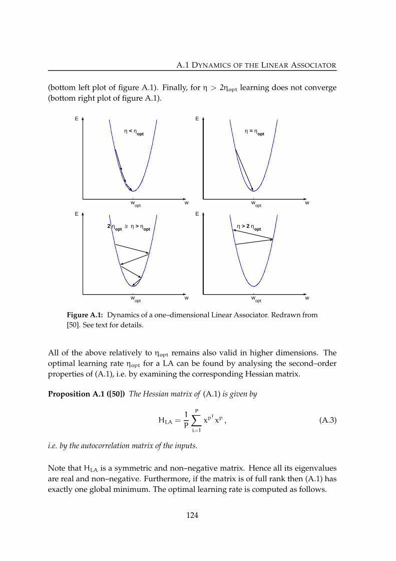
A.1 DYNAMICS OF THE LINEAR ASSOCIATOR
(bottom left plot of figure A.1). Finally, for η > 2ηopt learning does not converge
(bottom right plot of figure A.1).
E
w wopt
η < ηopt
E
w wopt
η = ηopt
E
w wopt
2 ηopt
≥ η > ηopt
E
w wopt
η > 2 ηopt
Figure A.1: Dynamics of a one–dimensional Linear Associator. Redrawn from
[50]. See text for details.
All of the above relatively to ηopt remains also valid in higher dimensions. The
optimal learning rate ηopt for a LA can be found by analysing the second–order
properties of (A.1), i.e. by examining the corresponding Hessian matrix.
Proposition A.1 ([50]) The Hessian matrix of (A.1) is given by
HLA =1
P
P∑
i=1
xpT
xp , (A.3)
i.e. by the autocorrelation matrix of the inputs.
Note that HLA is a symmetric and non–negative matrix. Hence all its eigenvalues
are real and non–negative. Furthermore, if the matrix is of full rank then (A.1) has
exactly one global minimum. The optimal learning rate is computed as follows.
124

APPENDIX A. SUPPLEMENTAL MATERIAL
Proposition A.2 ([50]) Let λmax and λmin denote the largest and smallest eigenvalue of
HLA, respectively. Then the optimal learning rate for a LA using gradient descent is
ηopt =1
λmax. (A.4)
The speed of convergence is proportional to
λmax
λmin. (A.5)
It is therefore desirable to have a small eigenvalue spread (A.5). If all eigenvalues
are equal then fastest convergence of learning is achieved. If additionally the co-
ordinate system spanned by the eigenvectors is in alignment with the coordinate
system of the data then convergence can be reached in one step. The alignment
of the two coordinate systems can always be forced by applying the appropriate
coordinate transformation to (A.1) [51]. In that new coordinate system the weight
update equations would be decoupled allowing to use a separate learning rate for
each direction. However, this is rather of theoretical interest since it practically
means to solve everything in advance.
125

A.2 UPDATE RULE FOR THE QUATERNIONIC SPINOR MLP
A.2 Update Rule for the Quaternionic Spinor MLP
For the Quaternionic Spinor MLP the weight update rule is given below1. The
notations used are that of section 5.1. Setting δ(l)
j as in (5.18) gives the update rule
for a weight in the output layer and setting δ(l)
j as in (5.27a) gives the update rule
for a weight in a hidden layer.
∆w(l)
kj =(
([δ(l)
j ]0w0x0+ ([δ(l)
j ]1(w0x1+w2x12−w12x2)
+ ([δ(l)
j ]2(w0x2−w1x12+w12x1) + ([δ(l)
j ]12(w0x12+w1x2−w2x1)e0)
+(
([δ(l)
j ]0w1x0+ ([δ(l)
j ]1(w1x1+w2x2+w12x12)
+ ([δ(l)
j ]2(w2x1−w0x12−w1x2) + ([δ(l)
j ]12(w12x1+w0x2−w1x12)e1)
+(
([δ(l)
j ]0w2x0+ ([δ(l)
j ]1(−w2x1+w1x2+w0x12)
+ ([δ(l)
j ]2(w1x1+w2x2+w12x12) + ([δ(l)
j ]12(w12x2−w0x1−w2x12)e2)
+(
([δ(l)
j ]0w12x0+ ([δ(l)
j ]1(w1x12−w0x2−w12x1)
+ ([δ(l)
j ]2(w0x1+w2x12−w12x2) + ([δ(l)
j ]12(w1x1+w2x2+w12x12)e12)
1Remember that updating the bias terms of a (S)CMLP is generic.
126

APPENDIX A. SUPPLEMENTAL MATERIAL
A.3 Some Elements of Clifford Analysis
This appendix provides some supplemented material on Clifford analysis which
was used in the discussion of universal approximation by Clifford MLPs in section
5.2. All the beneath is taken from [10].
In general (Cp,q)n is not a linear space. A module is a generalization of a linear
space, where the coefficients come from some ring (Cp,q) instead of a field.
Definition A.3 (Left Module) Let R be a ring with identity element 1. A left R-module
X is an Abelian group (X,+) together with a mapping R×X → X : (r, g) 7→ rg in such a
way, that
(a) ∀g1, g2 ∈ X ∀r ∈ R : r(g1+ g2) = rg1+ rg2
(b) ∀g ∈ X ∀r1, r2 ∈ R : (r1+ r2)g = r1g+ r2g
(c) ∀g ∈ X ∀r1, r2 ∈ R : (r1r2)g = r1(r2g)
(d) ∀g ∈ X : 1g = g
are fulfilled.
A left module may be equipped with a seminorm.
Definition A.4 (Seminorm) Let X be a left Cp,q-module. A function p : X → IR is called
a seminorm on X if it fulfills for all f, g ∈ X, λ ∈ Cp,q and κ ∈ IR
(a) p(f+ g) ≤ p(f) + p(g)
(b) p(f) = 0 ⇒ f = 0
(c) p(λf) ≤ C‖λ‖p(f)
p(κf) = |κ|p(f) .
A proper module is a left module equipped with a proper system of seminorms.
Definition A.5 (Proper Module) Let X be a left Cp,q-module. A family P of seminorms
p : X → IR is called a proper system of seminorms on X if for any finite sequence
p1, p2, . . . , pk ∈ P there exist p ∈ P and C > 0 such that for all f ∈ X
supj=1,...,k
pj(f) ≤ Cp(f) . (A.6)
After these preliminaries the Hahn–Banach theorem and the Riesz representation
theorem of Clifford analysis can be stated.
127

A.3 SOME ELEMENTS OF CLIFFORD ANALYSIS
Theorem A.6 (Hahn–Banach) Let X be a proper Cp,q-module, let Y be a submodule of
X and let T be a bounded left Cp,q-functional on Y. Then there exists a bounded left Cp,q-
functional T ∗ on X such that
T ∗|Y = T . (A.7)
Theorem A.7 (Riesz) LetX be a proper Cp,q-module, let T : X → Cp,q be a bounded linear
functional. Then there exists a unique Clifford measure µ on X such that for all continuous
f : X → Cp,q
〈T, f〉 =
∫
X
f dµ . (A.8)
128

Bibliography
[1] P. Arena, L. Fortuna, G. Muscato, and M. G. Xibilia. Neural Networks in Multi-
dimensional Domains. Number 234 in LNCIS. Springer–Verlag, 1998.
[2] P. Arena, L. Fortuna, R. Re, and M. G. Xibilia. Multilayer perceptrons to ap-
proximate complex valued functions. International Journal of Neural Systems,
6:435–446, 1995.
[3] P. F. Baldi and K. Hornik. Learning in linear neural networks: A survey. IEEE
Transactions on Neural Networks, 6(4):837–858, 1995.
[4] V. Banarer, C. Perwass, and G. Sommer. Design of a multilayered feed-forward
neural network using hypersphere neurons. In N. Petkov and M. A. West-
enberg, editors, Proc. 10th Int. Conf. Computer Analysis of Images and Patterns,
CAIP 2003, Groningen, The Netherlands, August 2003, volume 2756 of LNCS,
pages 571–578. Springer-Verlag, 2003.
[5] V. Banarer, C. Perwass, and G. Sommer. The hypersphere neuron. In 11th
European Symposium on Artificial Neural Networks, ESANN 2003, Bruges, pages
469–474. d-side publications, Evere, Belgium, 2003.
[6] A. Barron. Universal approximation bounds for superpositions of a sigmoidal
function. IEEE Transactions on Information Theory, 39:930–945, 1993.
[7] N. Benvenuto and F. Piazza. On the complex backpropagation algorithm.
IEEE Transactions on Signal Processing, 40(4):967–969, 1992.
[8] C. M. Bishop. Neural Networks for Pattern Recognition. Oxford University Press,
Oxford, 1995.
[9] H. Boulard and N. Morgan. Connectionist Speech Recognition. Kluwer, 1993.
[10] F. Brackx, R. Delanghe, and F. Sommen. Clifford Analysis. Pitman, London,
1982.
129

BIBLIOGRAPHY
[11] S. Buchholz and G. Sommer. A hyperbolic multilayer perceptron. In S.-I.
Amari, C.L. Giles, M. Gori, and V. Piuri, editors, International Joint Conference
on Neural Networks, IJCNN 2000, Como, Italy, volume 2, pages 129–133. IEEE
Computer Society Press, 2000.
[12] S. Buchholz and G. Sommer. Learning geometric transformations with Clif-
ford neurons. In G. Sommer and Y. Zeevi, editors, 2nd International Workshop
on Algebraic Frames for the Perception-Action Cycle, AFPAC 2000, Kiel, volume
1888 of LNCS, pages 144–153. Springer-Verlag, 2000.
[13] S. Buchholz and G. Sommer. Quaternionic spinor MLP. In 8th European Sym-
posium on Artificial Neural Networks, ESANN 2000, Bruges, pages 377–382, 2000.
[14] S. Buchholz and G. Sommer. Clifford algebra multilayer perceptrons. In Som-
mer [83], pages 315–334.
[15] S. Buchholz and G. Sommer. Introduction to neural computation in Clifford
algebra. In Sommer [83], pages 291–314.
[16] T. Caelli, D. Squire, and T. Wild. Model–based neural networks. Neural Net-
works, 6:613–625, 1993.
[17] A. Church. An unsolvable problem of elementary number theory. American
Journal of Mathematics, 58:345–363, 1936.
[18] T. Clarke. Generalization of neural network to the complex plane. Proc. of the
IJCNN, 2:435–440, 1990.
[19] W. K. Clifford. Preliminary scetch of bi–quaternions. Proc. London Math. Soc.,
4:381–395, 1873.
[20] J. Cnops. Hurwitz pairs and applications of Mobius transformations. Habilitation
dissertation, University of Gent, Belgium, 1994.
[21] B. J. Copeland. Artificial Intelligence: A Philosophical Introduction. Blackwell
Publishers, Oxford, 1993.
[22] K. J. W. Craik. The Nature of Explanation. Cambridge University Press, Cam-
bridge, 1943.
[23] G. Cybenko. Approximation by superposition of a sigmoidal function. Math-
ematics of Control, Signals and Systems, 2:303–314, 1989.
[24] K. Daniilidis. Using the algebra of dual quaternions for motion alignment. In
Sommer [83], pages 489–499.
130

BIBLIOGRAPHY
[25] B. Denby. The use of neural networks in high–energy physics. Neural Compu-
tation, 5:505–549, 1993.
[26] H. English and Y. Hiemstra. The correlation as cost function in neural net-
works. In Proc. of the IEEE WCCI, Orlando, pages 1370–1372, 1994.
[27] H.-D. Ebbinghaus et al. Numbers. Springer–Verlag, 3rd edition, 1995.
[28] B. G. Farley and W. A. Clark. Simulations of self–organizing systems by digital
computer. I.R.E. Transactions on Information Theory, 4:76–84, 1954.
[29] M. Ferraro and T. Caelli. Neural computation of algebraic and geometrical
structures. Neural Networks, 11:669–707, 1998.
[30] S. G. Gal. Introduction to Geometric Function Theory of Hypercomplex Variables.
Nova Science Publishers, New York, 2002.
[31] S. Geman, E. Bienenstock, and R. Doursat. Neural networks and the
bias/variance dilemma. Neural Computation, 4:1–58, 1992.
[32] G. Georgiou and C. Koutsougeras. Complex domain backpropagation. IEEE
Trans. on Circuits and Systems II, 39(5):330–334, 1992.
[33] W.R. Hamilton. Elements of Quaternions. Longmans Green, London 1866.
Chelsea, New York, 1969.
[34] S. J. Hanson and C. R. Olson. Neural networks and natural intelligence: Notes
from Mudville. Connection Science, 3:332–335, 1991.
[35] D. O. Hebb. The Organization of Behaviour. John Wiley & Sons, New York, 1949.
[36] R. Hecht-Nielsen. Neurocomputing. Addison–Wesley Publishing Company,
Inc., 1991.
[37] W. Hein. Struktur– und Darstellungstheorie der klassischen Gruppen. Springer–
Verlag, 1990.
[38] D. Hestenes. Space–Time Algebra. Gordon and Breach, New York, 1966.
[39] D. Hestenes. New Foundations for Classical Mechanics. D. Reidel Publishing,
Dordrecht, 1986.
[40] D. Hestenes and G. Sobczyk. Clifford Algebra to Geometric Calculus. D. Reidel
Publ. Comp., Dordrecht, 1984.
131

BIBLIOGRAPHY
[41] K. Hornik, M. Stinchcombe, and H. White. Multilayer feedforward networks
are universal approximators. Neural Networks, 2:359–366, 1989.
[42] L. Jones. A simple lemma on greedy approximation in Hilbert space and con-
vergence rates for projection pursuit regression and neural networks. Annals
of Statistics, 20:608–613, 1992.
[43] L. B. Kaelbling, M. L. Littman, and A. W. Moore. Reinforcement learning: A
survey. Journal of Artificial Intelligence Research, 4, 1996.
[44] T. Kim and T. Adali. Complex backpropagtion neural network using elemen-
tary transcendetal activation functions. Proc. of IEEE ICASSP, pages 1281–
1284, 2001.
[45] V. V. Kisil. Mobius transformations and monogenic Functional Calculus. Elec-
tronic Reasearch Announcements of the AMS, 2(1):26–33, 1996.
[46] S. C. Kleene. General recursive functions of natural numbers. Mathematische
Annalen, 112:727–742, 1936.
[47] A. N. Kolmogorov. On the representation of continous functions of several
variables by superposition of continous functions of one variable and addi-
tion. Doklady Akademiia Nauk SSSR, 114(5):953–956, 1957.
[48] V. Kurkova. Kolmogorov’s theorem is relevant. Neural Computation, 3(4):617–
622, 1991.
[49] V. Kurkova. Kolmogorov’s theorem and multilayer neural networks. Neural
Networks, 5(3):501–506, 1992.
[50] Y. LeCun, L. Bottou, G. B. Orr, and K.-R. Muller. Efficient BackProp. In G. B.
Orr and K.-R. Muller, editors, Neural Networks: Tricks of the Trade. Springer–
Verlag, 1998.
[51] Y. LeCun, I. Kanter, and S. A. Solla. Eigenvalues of covariance matrices: Appli-
cation to neural–network learning. Physical Review Letters, 66(18):2396–2399,
1991.
[52] L. R. Leerink, C. L. Giles, B. G. Horne, and M. A. Jabri. Learning with product
units. In G. Tesauro, D. Touretzky, and T. Leen, editors, Advances in Neural
Information Processing Systems, volume 7, pages 537–544. The MIT Press, 1995.
[53] M. Leshno, V. Y. Lin, A. Pinkus, and S. Schocken. Multliayer feedforward net-
works with a nonpolynomial activation function can approximate any func-
tion. Neural Networks, 6:861–867, 1993.
132

BIBLIOGRAPHY
[54] H. Leung and S. Haykin. The complex backpropagation algorithm. IEEE
Transactions on Signal Processing, 3(9):2101–2104, 1991.
[55] E. N. Lorenz. Deterministic nonperiodic flow. Journal Athmospheric Science,
20:130–134, 1963.
[56] P. Lounesto. Clifford Algebras and Spinors. Cambridge University Press, 1997.
[57] J. L. McClelland, D. E. Rumelhart, and the PDP research group, editors. Paral-
lel Distributed Processing, volume 2: Psychological and Biological Models. MIT
Press, Cambridge MA, 1986.
[58] W. S. McCulloch and W. Pitts. A logical calculus of ideas immanent in nervous
activity. Bulletin of Mathematical Biophysics, 5:115–133, 1943.
[59] M. L. Minsky and S. A. Papert. Perceptrons. MIT Press, 1969.
[60] T. Needham. Visual Complex Analysis. Clarendon Press, Oxford, 1997.
[61] T. Nitta. An extension of the back–propagation algorithm to complex num-
bers. Neural Networks, 10(8):1391–1415, 1997.
[62] J. K. Pearson. Clifford Networks. PhD thesis, University of Kent, 1994.
[63] A. Pellionisz and R. Llinas. Tensor network theory of the metaorganization of
functional geometries in the central nervous system. Neuroscience, 16(2):245–
273, 1985.
[64] C. Perwass, V. Banarer, and G. Sommer. Spherical decision surfaces using
conformal modelling. In B. Michaelis and G. Krell, editors, 25. Symposium fur
Mustererkennung, DAGM 2003, Magdeburg, volume 2781 of LNCS, pages 9–16.
Springer-Verlag, Berlin, 2003.
[65] A. Pinkus. Approximation theory of the mlp model in neural networks. Acta
Numerica, 8:143–195, 1999.
[66] P. Plucker. On a new geometry of space. Phil. Trans. R. Soc. London, 155, 1865.
[67] I. R. Porteous. Clifford Algebras and the Classical Groups. Cambridge University
Press, Cambridge, 1995.
[68] H. Pottmann and J. Wallner. Computational Line Geometry. Springer–Verlag,
2001.
133

BIBLIOGRAPHY
[69] H. Ritter, T. Martinetz, and K. Schulten. Neuronale Netze. Addison–Wesley,
Bonn, 1990.
[70] R. Rojas. Neural Networks. Springer–Verlag, 1996.
[71] J. Rooney. A Comparison of Representations of General Screw Displacements.
Environment and Planning B, 5:45–88, 1978.
[72] F. Rosenblatt. The perceptron: A probalistic model for information storage
and organization in the brain. Psycol. Rev., 65:386–408, 1958.
[73] F. Rosenblatt. Principles of Neurodynamics. Spartan, New York, 1962.
[74] B. Rosenhahn. Pose estimation revisited. Technical Report Number 0308,
Christian-Albrechts-Universitat zu Kiel, Institut fur Informatik und Prak-
tische Mathematik, September 2003.
[75] W. Rudin. Real and Complex Analysis. McGraw–Hill, New York, 1966.
[76] D. E. Rumelhart, G. E. Hinton, and R. J. Williams. Learning internal represen-
tations by error propagation. In Rumelhart et al. [77], pages 318–362.
[77] D. E. Rumelhart, J. L. McClelland, and the PDP research group, editors. Paral-
lel Distributed Processing, volume 1: Foundations. MIT Press, Cambridge MA,
1986.
[78] A. E. Samuel, P. R. McAree, and K. H. Hunt. Unifying screw geometry and
matrix transformation. International Journal of Robotics Research, 10(5):454–472,
1991.
[79] F. Scarselli and A. C. Tsoi. Universal approximation using feedforward neural
networks: A survey of some existing methods, and some new results. Neural
Networks, 11(1):15–37, 1998.
[80] V. G. Shervatov. Hyperbolic Functions. D.C. Heath and Company, Boston, 1963.
[81] B. F. Skinner. The Behavior of Organisms: An Experimental Analysis. Appleton–
Century–Crofts, New York, 1938.
[82] G. Sommer. Algbraic aspects of designing behavior based systems. In G. Som-
mer and J. J. Koenderink, editors, Proc. Int. Workshop AFPAC’97, vol. 1315 of
LNCS, pages 1–28. Springer–Verlag, 1997.
[83] G. Sommer, editor. Geometric Computing with Clifford Algebras. Springer–
Verlag, 2001.
134

BIBLIOGRAPHY
[84] E. Study. Geometrie der Dynamen. Leipzig, 1903.
[85] E. L. Thorndike. The Fundamentals of Learning. Teachers College Press, New
York, 1933.
[86] A. M. Turing. On computable numbers, with an application to the Entschei-
dungsproblem. Proceedings of the London Mathematical Society, 42:230–265,
1936.
[87] K. Th. Vahlen. Ueber Bewegungen und complexe Zahlen. Math. Ann., 55:585–
593, 1902.
[88] V. Vapnik. The Nature of Statistical Learning Theory. Springer–Verlag, New York,
1995.
[89] M. Vidyasagar. A Theory of Learning and Generalization. Springer–Verlag, 1997.
[90] K. Voss and H. Susse. Adaptive Modelle und Invarianten fur zweidimensionale
Bilder. Verlag Shaker, Aachen, 1995.
[91] H. White. Connectionist nonparametric regression: multilayer feedforward
networks can learn arbitrary mappings. Neural Networks, 3(5):543–549, 1990.
[92] I. H. Witten and E. Frank. Data Mining: Practical Machine Learning Tools and
Techniques with Java Implementations. Academic Press, 2000.
[93] I. M. Yaglom. Complex Numbers in Geometry. Academic Press, New York, 1968.
135