› teses › disponiveis › 55 › 55134 › tde... · Pedro Augusto Munari Junior Advisor: Prof....

Theoretical and computational issues for improving the performance of linear optimization methods

Pedro Augusto Munari Junior

Theoretical and computational issues for improving the performance of linear optimization methods1


Advisor: Prof. Marcos Nereu Arenales.

Co-advisor: Prof. Jacek Gondzio.

Doctoral dissertation submitted to the Instituto de

Ciências Matemáticas e de Computação - ICMC-USP, in partial fulfillment of the requirements for the degree of the Doctorate Program in Computer Science and Computational Mathematics. FINAL VERSION.

USP – São Carlos

April 2013

1 This research was supported by FAPESP (São Paulo Research Foundation) and CAPES Foundation.

SERVIÇO DE PÓS-GRADUAÇÃO DO ICMC-USP

Data de Depósito: Assinatura:________________________

Ficha catalográfica elaborada pela Biblioteca Prof. Achille Bassi e Seção Técnica de Informática, ICMC/USP,

com os dados fornecidos pelo(a) autor(a)

M963tMunari Junior, Pedro Augusto Theoretical and computational issues forimproving the performance of linear optimizationmethods / Pedro Augusto Munari Junior; orientadorMarcos Nereu Arenales; co-orientador Jacek Gondzio. -- São Carlos, 2013. 119 p.

Tese (Doutorado - Programa de Pós-Graduação emCiências de Computação e Matemática Computacional) --Instituto de Ciências Matemáticas e de Computação,Universidade de São Paulo, 2013.

1. Otimização linear. 2. Métodos tipo simplex. 3.Métodos de pontos interiores. 4. Geração de colunas.5. Branch-price-and-cut. I. Arenales, Marcos Nereu,orient. II. Gondzio, Jacek, co-orient. III. Título.

Aspectos teóricos e computacionais para a melhoria do desempenho de métodos de otimização linear


Aspectos teóricos e computacionais para a melhoria do desempenho de métodos de otimização linear1


Orientador: Prof. Marcos Nereu Arenales

Co-orientador: Prof. Jacek Gondzio

Tese apresentada ao Instituto de Ciências Matemáticas e de Computação - ICMC-USP, como parte dos requisitos para obtenção do título de Doutor em Ciências - Ciências de Computação e Matemática Computacional. VERSÃO REVISADA.

USP – São Carlos

Abril de 2013

1 Este trabalho foi financiado pela Fundação de Amparo à Pesquisa do Estado de São Paulo (FAPESP) e pela Coordenação de Aperfeiçoamento de Pessoal de Nível Superior (CAPES).

SERVIÇO DE PÓS-GRADUAÇÃO DO ICMC-USP

Data de Depósito: Assinatura:________________________

Ficha catalográfica elaborada pela Biblioteca Prof. Achille Bassi e Seção Técnica de Informática, ICMC/USP,

com os dados fornecidos pelo(a) autor(a)

M963tMunari Junior, Pedro Augusto Theoretical and computational issues forimproving the performance of linear optimizationmethods / Pedro Augusto Munari Junior; orientadorMarcos Nereu Arenales; co-orientador Jacek Gondzio. -- São Carlos, 2013. 119 p.

Tese (Doutorado - Programa de Pós-Graduação emCiências de Computação e Matemática Computacional) --Instituto de Ciências Matemáticas e de Computação,Universidade de São Paulo, 2013.

1. Otimização linear. 2. Métodos tipo simplex. 3.Métodos de pontos interiores. 4. Geração de colunas.5. Branch-price-and-cut. I. Arenales, Marcos Nereu,orient. II. Gondzio, Jacek, co-orient. III. Título.

This thesis is dedicated to Alan Turing, the father of computer science.

His story shows how much the mankind lose with the prejudice.

As a scientist, his work goes beyond the machine.

As a man, his life goes beyond the human.

Acknowledgements

First of all, I thank God for giving me strength and perseverance to conduct my research.He was the only company in many sleepless nights and di�cult times. Thanks to Him, Ibelieved I could accomplish this doctoral degree. I am very thankful to my mother and myfather for being amazing parents, giving me all the support and respecting my decisions. Iam grateful to all my closest friends, who brings shine and happiness to my life. Specialthanks to Douglas, Deise, Flavinha, and Gustavo. I am very grateful to Felipe, who has beena wonderful partner.

Many thanks to Prof. Arenales for guiding this research and for being so kind and sup-portive during all these years. I have learned from him not only about optimization, but alsoabout life. I am very thankful to Prof. Jacek for accepting me as visitor at the University ofEdinburgh and for being such a fantastic supervisor all the time. I really admire him as alecturer, as a supervisor, as a friend and specially as a person. He taught me how to conductmy research seriously, and I am indebted to him because of that.

Thanks to the lecturers and professors of the ICMC/University of São Paulo. Specialthanks to Prof. Franklina for helping me with several di�culties and for being so kind andrespectful all the time. Thanks to all my friends and colleagues from the Optimization Labo-ratory (LOT) at the University of São Paulo, who made all the years we have spent togethermuch happier and easier. A special thanks to Aline, Claudia, Douglas, Lana, Murilo, Pamela,Tamara and Victor, with whom I have shared most of my moments. I have learned a lot fromthem. Thanks to all my friends and colleagues from the University of Edinburgh as well, inspecial to Chris, George, Marina, Pablo and Pamela. They made my life in Scotland muchwarmer. I am also very thankful to Elizabeth, who was a very special friend in Edinburghand is (fortunately) back in Brazil. I am also thankful to all the sta� from the University ofSão Paulo and the University of Edinburgh.

I am grateful to the thesis examiners committee, namely Prof. Aurélio Ribeiro Oliveira,Prof. José Manuel Valério de Carvalho, Prof. Marcos Poggi de Aragão and Prof. MaristelaSantos, for their valuable contributions to this thesis. I also thank the University of São Pauloand the Brazilian research funding councils FAPESP (São Paulo Research Foundation) andCAPES Foundation for all the support.

Abstract

Linear optimization tools are used to solve many problems that arise in our day-to-day lives.The linear optimization models and methodologies help to �nd, for example, the best amountof ingredients in our food, the most suitable routes and timetables for the buses and trainswe take, and the right way to invest our savings. We would cite many other situations thatinvolves linear optimization, since a large number of companies around the world base theirdecisions in solutions which are provided by the linear optimization methodologies. In thisthesis, we propose theoretical and computational developments to improve the performanceof important linear optimization methods. Namely, we address simplex type methods, inte-rior point methods, the column generation technique and the branch-and-price method. Insimplex-type methods, we investigate a variant which exploits special features of problemswhich are formulated in the general form. We present a novel theoretical description of themethod and propose how to e�ciently implement this method in practice. Furthermore, wepropose how to use the primal-dual interior point method to improve the column generationtechnique. This results in the primal-dual column generation method, which is more sta-ble in practice and has a better overall performance in relation to other column generationstrategies. The primal-dual interior point method also o�ers advantageous features which canbe exploited in the context of the branch-and-price method. We show that these featuresimproves the branching operation and the generation of columns and valid inequalities. Forall the strategies which are proposed in this thesis, we present the results of computationalexperiments which involves publicly available, well-known instances from the literature. Theresults indicate that these strategies help to improve the performance of the linear optimiza-tion methodologies. In particular for a class of problems, namely the vehicle routing problemwith time windows, the interior point branch-and-price method proposed in this study wasup to 33 times faster than a state-of-the-art implementation available in the literature.

Keywords: linear optimization; simplex type methods; interior point methods; column gen-eration; branch-and-price.

Resumo

Ferramentas de otimização linear são usadas para resolver diversos problemas do nosso dia-a-dia. Os modelos e as metodologias de otimização linear ajudam a obter, por exemplo, amelhor quantidade de ingredientes na nossa alimentação, os horários e as rotas de ônibus etrens que tomamos, e a maneira certa para investir nossas economias. Muitas outras situ-ações que envolvem otimização linear poderiam ser aqui citadas, já que um grande númerode empresas em todo o mundo baseia suas decisões em soluções obtidas pelos métodos deotimização linear. Nesta tese, são propostos desenvolvimentos teóricos e computacionais paramelhorar o desempenho de métodos de otimização linear. Em particular, serão abordadosmétodos tipo simplex, métodos de pontos interiores, a técnica de geração de colunas e ométodo branch-and-price. Em métodos tipo simplex, é investigada uma variante que exploraas características especiais de problemas formulados na forma geral. Uma nova descriçãoteórica do método é apresentada e, também, são propostas técnicas computacionais para aimplementação e�ciente do método. Além disso, propõe-se como utilizar o método primal-dualde pontos interiores para melhorar a técnica de geração de colunas. Isto resulta no métodoprimal-dual de geração de colunas, que é mais estável na prática e tem melhor desempenhogeral em relação a outras estratégias de geração de colunas. O método primal-dual de pontosinteriores também oferece características vantajosas que podem ser exploradas em conjuntocom o método branch-and-price. De acordo com a investigação realizada, estas característicasmelhoram a operação de rami�cação e a geração de colunas e de desigualdades válidas. Paratodas as estratégias propostas neste trabalho, são apresentados os resultados de experimentoscomputacionais envolvendo problemas de teste bem conhecidos e disponíveis publicamente.Os resultados indicam que as estratégias propostas ajudam a melhorar o desempenho dasmetodologias de otimização linear. Em particular para uma classe de problemas, o problemade roteamento de veículos com janelas de tempo, o método branch-and-price de pontos interi-ores proposto neste estudo foi até 33 vezes mais rápido que uma implementação estado-da-artedisponível na literatura.

Palavras-chave: Otimização linear; métodos tipo simplex; métodos de pontos interiores;geração de colunas, branch-and-price.

��

� ��

��

��

��

��

��

�� !��

�� "�� #��

�� $�� #��

��% &�� %

� � ��

�� '��

�� (

� ) ��*�� +��

�% !�� +�� ,

�, "�� +�� -�� .

�� &� �� %%

�� !�� %%

�� /�� +�� %,

�� %.

��% 0� �� %�

�. /�� %�

�.�� &�� +�� -�� %(

�.�� &� �� #�� ,�

�� &�� ,�

� ��

��

%�� "�� ,�

%�� 1��

%� "�� #��

%�% &� ��

%�%�� &�� +��

%�%�� 1�� +�� .�

%�%� &�� 2��#��3�� +�� "� �� .�

%�%�% �� .%

%�, &�� .,

� ��

��

,�� )�� .�

,�� 4�� +��#��#��#��

,�� #��

,�� #��

,��

,��% ��

,��, $�� %

,� "�� *�� +�� 51/�"$6 � � � � � � � � � � �,

,� �� 7�� ,

,� �� *�� 7��/& � � � � � � � � � � � � � � � � � � � � � � � � � � � � �.

,� � 1�� 8�� 1/�"$ � � � � � � � � � � � � � � � � � � � � �(

,� �% �� 1/�"$ � � � � � � � � � � � � � � � � � � � � � � � � (�

,�% &� �� (�

,�%�� #+�� (�

,�%�� ) �� (%

,�, &�� (.

!�� ""

� #�� $ ��%��&�� '�

�� !$! �� +��

�� 78��*�� 2�� %

�� 7�� !$! � � � � � � � � � � � � � � � � � � � � � � � � � � ��,

�� &�� +�� ,

�� 1�� +�� .

�� &�� 2��#��3�� +�� "� �� (

List of Tables

3.1 Numerical tolerances used in our computational implementation. . . . . . . . . . . 493.2 Description of the Netlib instances. (Part 1) . . . . . . . . . . . . . . . . . . . . . 503.3 Description of the Netlib instances. (Part 2) . . . . . . . . . . . . . . . . . . . . . 513.4 Number of iterations and CPU time (in seconds) to solve the Netlib instances by using

two variants of the dual simplex method for problems in the general form: one using

the standard ration test (DSMGF-SRT) and another using the bound �ipping ratio

test (DSMGF-BFRT). (Part 1) . . . . . . . . . . . . . . . . . . . . . . . . . . . . 533.5 Number of iterations and CPU time (in seconds) to solve the Netlib instances by using

two variants of the dual simplex method for problems in the general form: one using

the standard ration test (DSMGF-SRT) and another using the bound �ipping ratio

test (DSMGF-BFRT). (Part 2) . . . . . . . . . . . . . . . . . . . . . . . . . . . . 543.6 Number of iterations and CPU time (in seconds) to solve the Netlib instances by using

three simplex type methods: the primal simplex method for problems in the standard

form (PSMSF), the dual simplex method for problems in the standard form (DSMSF),

and the dual simplex method for problems in the general form (DSMGF). (Part 1) . 553.7 Number of iterations and CPU time (in seconds) to solve the Netlib instances by using

three simplex type methods: the primal simplex method for problems in the standard

form (PSMSF), the dual simplex method for problems in the standard form (DSMSF),

and the dual simplex method for problems in the general form (DSMGF). (Part 2) . 56

4.1 Average results on the 262 CSP instances using di�erent values for k (maximumnumber of columns added to the RMP at a time). . . . . . . . . . . . . . . . . 69

4.2 Results on 14 large CSP instances (with k = 100). . . . . . . . . . . . . . . . 704.3 Average results on 220 CSP instances from triplet and uniform problem sets

(using k = 100). . . . . . . . . . . . . . . . . . . . . . . . . . . . . . . . . . . . 704.4 Average results on 87 VRPTW instances adding at most k columns at a time. 714.5 Results on 9 large VRPTW instances adding 300 columns at a time. . . . . . 724.6 Average results on 751 CLSPST instances. . . . . . . . . . . . . . . . . . . . . 734.7 Average results on 44 CLSPST large instances. . . . . . . . . . . . . . . . . . 74

5.1 Parameter choices in the IPBPC implementation for the VRPTW . . . . . . . 925.2 IPBPC results for the 100-series Solomon's instances. . . . . . . . . . . . . . . 935.3 IPBPC results for the 200-series Solomon's instances. . . . . . . . . . . . . . . 945.4 Comparison to a simplex-based BPC method (100-series Solomon's instances). 955.5 Comparison to a simplex-based BPC method (200-series Solomon's instances). 96

List of Figures

2.1 Illustration of the points that are visited by a simplex-type method. The fea-sible set is represented by the colored region. The vertices of the region arehighlighted by the (yellow) balls on its boundary. A simplex type method visitsa sequence of vertices, following the (red) dashed arrows (for example). . . . . 9

2.2 Illustration of the positive orthant in the space of pairwise products, with n = 2. 17

2.3 Narrow neighborhood in the space of pairwise products with the duality mea-sures of iterations k and k + p (the set F0 is not represented in the illustration). 18

2.4 Wide neighborhood in the space of pairwise products with the duality measuresof iterations k and k + p (the set F0 is not represented in the illustration). . . 18

2.5 Symmetric neighborhood in the space of pairwise products with the dualitymeasures of iterations k and k+p (the set F0 is not represented in the illustration). 18

2.6 The two main concerns when warmstarting the primal-dual interior point method:(a) Feasibility of the primal and dual constraints; (b) Nonnegativity and cen-trality. . . . . . . . . . . . . . . . . . . . . . . . . . . . . . . . . . . . . . . . 22

2.7 One-phase warmstarting techniques in the space of pairwise products. Thepositive orthant is expanded so that all points represented in Fig. 2.6 becomesuitable initial points. . . . . . . . . . . . . . . . . . . . . . . . . . . . . . . . 22

2.8 Two-phase warmstarting techniques in the space of pairwise products. Thevector of adjustments is computed so that the bad points represented in Fig.2.6 become suitable initial points after using the adjustments. . . . . . . . . . 22

3.1 Di�erent plots of the function hj(yj), according to the bounds lj and uj , j ∈ J . . . 29

3.2 Illustration of the bevahior of the dual objective function according to the variation of

the step-size εD. (a) Dual objective function h(y) with breakpoints at εD = εD1 and

εD = εD2 . (b) Function hBp(yBp

) with yBpas a function of εD. (c) Function hBr

(yBr)

with yBras a function of εD. . . . . . . . . . . . . . . . . . . . . . . . . . . . . . 39

3.3 Illustration of Theorem 3.5.1 with t = 4, k = 3 and P+i ∈ Ib, for i = 1, . . . , 4.

The breakpoints εD1 , . . . , εD4 are determined by the changes of the sign of components

yP+1, . . . , yP+

4. After εD = εD3 , h(y) decreases as εD increase, which indicates that εD3

is the step-size that leads to the largest improvement in the value of the objective

function. . . . . . . . . . . . . . . . . . . . . . . . . . . . . . . . . . . . . . . . 42

3.4 Data structure that stores the permuted triangular factors. . . . . . . . . . . . . . 48

4.1 Illustration of the unstable behavior of the optimal solutions in four subsequentouter iterations of the standard column generation method. . . . . . . . . . . 61

4.2 Illustration of the behavior of the well-centered, suboptimal solutions in twosubsequent outer iterations of the primal-dual column generation method. . . 64

4.3 Illustration of the dual solutions used by each column generation variant. . . . 68

5.1 Impact of changing the early branching threshold εb. . . . . . . . . . . . . . . 965.2 Impact of changing the separation subproblem threshold εc. . . . . . . . . . . 97

A.1 The coe�cient matrix that has the special structure which is suitable for ap-plying the DWD. . . . . . . . . . . . . . . . . . . . . . . . . . . . . . . . . . . 102

Chapter 1

Introduction

Information systems have evolved from simple data-management softwares to complex frame-works. Currently, some of them are able to execute very di�cult tasks such as �nding the besttimetable for a public transportation system, suggesting a disease treatment, and forecastingnatural disasters. To achieve such status, the advances in hardware and software engineeringare important, as they allow computers to be more and more e�cient after each year. But,in addition to that, complex systems rely on strong theoretical developments in mathematics,physics and related sciences. These developments allow real-life problems to be representedby mathematical models which are suitable for cleverly designed algorithms. Linear optimiza-tion is a successful example of a theoretical subject that is nowadays crucial to many complexinformation systems.

By linear optimization we refer to the theory and methods related to minimizing (ormaximizing) a given linear function, which is restricted to a domain that is fully described bya set of linear equations or inequalities. Many real-life problems can be represented this way,in particular those faced by manufacturing companies, transportation and telecommunicationbusinesses, and �nancial markets. The key point in the linear optimization is that the problemscan be formulated by a relatively simple mathematical language, and powerful computationalmethods are available to tackle these formulations.

The linear optimization is typically divided into two main subjects: linear programming

and integer programming. In the former, the domain of the function we are interested inoptimizing is continuous. It is useful when we are looking for solutions which can be statedas fractional amounts, e.g., when we want to know how much money to invest in a project,or what is the best proportion of ingredients in a blending. On the other hand, the integerprogramming is used when problems require decisions that can only be represented by integervalues, so the domain of the function must be discrete. This case involves the search fordecisions such as how many vehicles a company should use to deliver goods, which region isthe best for setting a warehouse. It can also involve cases in which the solutions have discreteas well as fractional decisions, e.g. in a set of projects to invest, which one we should selectand how much money we should assign to them.

The linear programming ideas started to be formalized during the Second World War,due to the need for e�cient allocation of resources. The subject called the attention ofthe community when George B. Dantzig proposed the simplex method in 1947, a practicalalgorithm to solve linear programming formulations (Dantzig, 1951). With this method, small-size problems were solved even by using calculators. The �rst computational implementationsof the method were very promising and motivated the investigation of e�cient techniques toimprove the performance of the method (Dantzig and Orchard-Hays, 1954; Orchard-Hays,1968; Maros, 2003a). Until the beginning of the Eighties, simplex-type methods were still the

1

only practical methods available to solving linear programming problems. Then, the projectiveinterior point method proposed by Karmarkar (1984) started a new age in linear programming.It was the �rst polynomial time algorithm for linear programming that was announced to bee�cient in practice as well. Previous to Karmarkar's method, Khachiyan (1979) had proposedan algorithm for linear programming with polynomial complexity as well, but with poorcomputational performance in practice. The theoretical and practical issues of the interiorpoint methods used nowadays are di�erent from those presented by Karmarkar. Nevertheless,the author is recognized for having called the attention of the optimization community to anew methodology, which stimulated an intense research in the area. The developments ininterior point methods stimulated at the same time the investigation for e�cient techniquesto improve simplex-type methods, in order to keep these methods competitive in practice.As a consequence, important achievements were accomplished for these linear programmingmethodologies, and the methods became able to solve larger and larger problems (Bixby etal., 1992; Bixby, 2002; Maros, 2003a; Gondzio and Grothey, 2006; Gondzio, 2012).

Currently, simplex-type methods and interior point methods are the dominant linear pro-gramming methodologies. These are powerful general-purpose methods that are available inthe majority of the optimization softwares as well as information systems that need to op-timize linear models. The free software COIN-OR (COIN-OR Foundation, Inc., 2012) andthe commercial software CPLEX (IBM ILOG CPLEX v.12.1, 2010) are examples of packageswhich o�er e�cient implementations of the simplex method, in its primal and dual versions,and the primal-dual interior point method. It is important to have both methods availablebecause they may show di�erent performances on di�erent classes of problems. The bestmethod depends on issues related to the dimensions of the model, the structure and sparsityof the coe�cient matrix, among others. As a consequence, it is di�cult to ensure in advancewhich method will be the best for an speci�c problem. See Bixby (2002) for a computationalstudy that compares implementations of these methods.

The integer programming �eld emerged from the need to obtain solutions with integervalued amounts. The simplex method was able to optimize general-purpose linear formula-tions that were restricted to continuous domains only. Until the mid-Fifties, there was nocomputational method able to guarantee optimal integer solutions to general-purpose integerprogramming models. Fortunately, this scenario changed with the introduction of the cuttingplane method by Gomory (1958). The strategy was based on iteratively inserting cuts (linearinequalities) to the formulation after solving it by the simplex method. A couple of years later,Land and Doig (1960) came up with a completely di�erent approach for obtaining optimalsolutions for integer programming problems: the branch-and-bound method. Interestinglyenough, these two methods are still nowadays the most used to solve integer programmingformulations. The combination of these two approaches results in the branch-and-cut method,which is currently the only general-purpose integer programming methodology available in op-timization softwares. For instance, powerful implementations of the branch-and-cut methodare available in the softwares cited above (COIN-OR and CPLEX).

Another important integer programming methodology is the branch-and-price method.It consists in the combination of the branch-and-bound method with a linear programmingmethodology that is called the column generation method. Ford and Fulkerson (1958) pro-posed the column generation method motivated by a linear programming problem whichwas too large to be stored in the computer memory. Since then, the column generation hasbeen applied to solve many problems, specially when combined with the branch-and-boundmethod. Di�erently form the branch-and-cut method, the implementation of a branch-and-price method is speci�c to solve a given problem. General-purpose implementations of thismethod are currently experimental (Galati et al., 2012; Lübbecke, 2012).

2

In this thesis, we investigate new strategies to improve the computational performanceof linear optimization methodologies. In linear programming, we present contributions re-garding its two main methodologies. We address a variant of the dual simplex method whichshows better performance on formulations which have lower and upper bounds for variablesand constraints. In addition, we show the advantageous features of using the primal-dualinterior point method within the column generation method. This research also contributeswith integer programming methodologies. In particular, we propose how to improve the per-formance of a branch-price-and-cut method by using the primal-dual interior point algorithm.To verify the behavior of the strategies that are proposed in this thesis, we use benchmark-ing instances that are available in public repositories and have been widely used in otherresearches. Besides, classical integer programming problems are addressed in the computa-tional experiments. In a class of problems, namely the vehicle routing problem with timewindows, the interior point branch-price-and-cut method proposed in this study was up to 33times faster than a state-of-the-art implementation of a standard branch-price-and-cut.

The remaining chapters in this thesis have the following description:

• Chapter 2: we brie�y describe the main linear programming methodologies, namelysimplex-type methods and the interior point methods. The purpose is to introduce themain aspects of each method and setting up the notation and background informationfor the remaining chapters. In addition, we propose a uni�ed framework to describesimplex type methods and interior point methods. This framework helps to show thedi�erences as well as the similarities regarding these methods. We also brie�y discussthe main ideas which are used to warmstart the primal-dual interior point method.

• Chapter 3: we further investigate a variant of the dual simplex method, which is de-signed for problems formulated in the general form. We present a novel theoreticaldescription of the method, which extends the results of previous studies. Furthermore,we describe computational techniques that lead to the e�cient implementation of themethod. To verify the performance of the proposed variants, we present the main resultsof computational experiments using the Netlib instances.

• Chapter 4: we address the use of the primal-dual interior point algorithm within thecolumn generation method. The motivation is given by the well-centered dual solu-tions that are o�ered by the interior point method. These solutions are more stablethan the optimal dual solutions that are often obtained by a simplex-type algorithmin the standard column generation method. The resulting variant, which we call asthe primal-dual column generation method, shows a better overall performance whencompared to the standard column generation. We prove the �nite convergence of themethod and show the results of extensive computational experiments. The performanceof the proposed approach is compared against the performance of two other variants ofthe column generation method. We used the linear relaxations of three classical integerprogramming problems in the experiments, namely the cutting stock problem, the ve-hicle routing problem with time windows, and the capacitated lot sizing problem withsetup times. The results indicate that the proposed variant achieves the best overallperformance regarding number of iterations and total CPU time in relation to othercolumn generation variants from the literature. In addition, the relative performance ofthe method was even better for classes of larger instances.

• Chapter 5: we propose how to improve the performance of a branch-price-and-cutmethod by using advantageous features that are o�ered by the primal-dual interior

3

point algorithm. In particular, two features are important in this context: (i) the well-centered primal and dual solutions o�ered by the interior point method are bene�cialto generate columns and valid inequalities; (ii) the early termination of the methodleads to suboptimal solutions that are good approximations of optimal solutions, whichcontributes with the branching operation and with the generation of valid inequalitiesas well. We discuss in detail how to deal with the challenges of integrating the interiorpoint algorithm with each core component of the branch-price-and-cut method. Theperformance of the proposed interior point branch-price-and-cut method was veri�ed inwell-known instances of the vehicle routing problem with time windows. The resultscon�rm that the proposed approach is robust and delivers the best overall performancewhen compared against the results of a state-of-the-art standard branch-price-and-cutmethod available in the literature.

The aim of this research is to contribute with the state-of-the-art in linear optimizationmethodologies. Furthermore, it allows the improvement of the information systems that arebased on linear optimization methodologies and, hence, it can be bene�cial to organizationsthat rely on these systems to make decisions. The simplex method was recognized as oneof the ten most in�uential algorithms to sciences and engineering (Dongarra and Sullivan,2000). The literature estimates that the simplex method is called around thousands of timesper second in softwares around the world (Elwes, 2012). Interior point methods are not farfrom this usage, and they have the additional advantage of being also applied to problems thatcannot be modeled by means of linear functions only (Nemirovski and Todd, 2008; Gondzio,2012). In other words, interior point methods can be used to solve a broader range of models,in which more complex features can be absorbed in the model by using, e.g., quadratic andlogarithmic functions. Finally, the column generation and the branch-and-price methods arecurrently the only methodologies which are able to �nd optimal solutions, in a reasonableamount of time, of important classes of problems in areas such as manufacturing and logistics(Lübbecke and Desrosiers, 2005; Desrosiers and Lübbecke, 2010).

4

Chapter 2

Linear programming methodologies

Linear programming is important for solving problems that emerges from di�erent situations.It o�ers intuitive formulations which are based on linear functions and linear systems of equa-tions/inequalities. Currently, these formulations can be solved by e�cient implementations ofcleverly designed linear programming methods. In addition, the linear programming method-ologies are often used as auxiliary tools for solving more complex problems. For instance, mostof the integer programming methodologies rely on linear programming to solve relaxations ofthe problem. The solutions which are obtained from the relaxations guide the search for anoptimal integer solution. Nonlinear programming and nondi�erentiable optimization are alsoexamples of areas that demand the linear programming methodologies.

Currently the most e�cient methodologies in linear programming are divided into twoclasses, namely the simplex-type methods and the interior point methods. The former consistsin variants of the pioneering method in the area, the (primal) simplex method (Dantzig, 1951).The latter is given by methods which are motivated by nonlinear programming techniques,following the projective interior point method (Karmarkar, 1984). Since their �rst proposals,these two methods have been continuously improved. It has been a very active research area,not only due to theoretical developments, but also because of the search for techniques thatresults in e�cient implementations of the methods. The main motivation lies in the factthat many other areas bene�t from improvements in the linear programming methodologies,as mentioned in the previous paragraph. As a result of this intense research, simplex type-methods and interior point methods are very competitive nowadays. It is di�cult to guesswhich method will solve a given linear programming problem with the best performance(Bixby, 2002; Gondzio, 2012). The dual simplex method is recognized for its best overallperformance in relation to other simplex-type methods (Koberstein, 2008). Regarding interiorpoint methods, the primal-dual interior point method is the most e�cient variant in general(Gondzio, 2012).

In this chapter, we brie�y review the linear programming methodologies, as they areaddressed in the remaining chapters of this thesis. The purpose is to provide a self-containeddescription of the methodologies as well as to set a standard notation. In addition, we proposea uni�ed framework to describe simplex type methods and interior point methods. Usually,these two methodologies are described by using very di�erent notations, as if they were notrelated at all. In spite of being essentially di�erent, these methods have certain similaritiesand, hence, they can be represented by a uni�ed linear programming framework. In Section2.2, we present the main ideas of simplex-type methods and then describe two importantvariants, the primal simplex method and the dual simplex method. In Section 2.3, we describe

5

the primal-dual interior point method and brie�y discuss how to warmstart this method.We assume the reader is familiar with the linear programming subject. For a thoroughintroduction to linear programming we suggest the textbooks by Bertsimas and Tsitsiklis(1997); Arenales et al. (2007).

2.1 A uni�ed framework for linear programming

Consider a linear programming problem which is formulated in the following standard form

(P ), together with its associated dual formulation (D),

(P ) min cTxs.t. Ax = b

x ≥ 0,

(D) max bT ys.t. AT y + s = c

s ≥ 0,(2.1)

where A is an m × n matrix with rank(A) = m, 0 < m ≤ n, x ∈ Rn is the vector of primalvariables, y ∈ Rm and s ∈ Rn are the vectors of dual variables. The parameters c ∈ Rnand b ∈ Rm are the costs vector and the right-hand side vector, respectively. We representthe columns of A by the vectors aj ∈ Rm, j = 1, . . . , n. Formulation (P ) is referred to asthe primal, to distinguish it from the dual (D). The linear function cTx is called the primal

objective function, while bT y is the dual objective function.Any linear programming can be formulated in the standard form (2.1). Due to this simplic-

ity, this formulation is typically adopted in textbooks and introductory texts regarding linearprogramming. Nevertheless, other types of formulations can be used to represent a problemequivalently. These alternative formulations are bene�cial to special contexts and they mayavoid the use of additional variables and/or constraints. For instance, in the literature aboutcomputational implementations of simplex type methods, a bounded variable formulation ispreferred because it express explicitly the lower and upper bounds of the primal variables.Thus, it helps to describe the implementation issues in a more realistic way. In practice, alinear programming problem may require lower and upper bounds to be imposed to certainconstraints. In such case, the general form can be used to formulate the problem, withouthaving to add any slack nor surplus variables. As we show in Chapter 3, this formulationo�ers advantageous features which can be exploited in order to obtain a variant of the dualsimplex method.

Let P = {x ∈ Rn | Ax = b, x ≥ 0} be the primal feasible set, i.e., the set of all thepoints that satis�es the constraints of (P ). If P = ∅, then the primal problem is infeasible.Otherwise, there exists at least one feasible point x in P. In addition, if cTx→ −∞, i.e., forany point x ∈ P it is possible to obtain another point x ∈ P such that cT x < cTx, then theprimal problem is unbounded. Otherwise, if there exists a point x? ∈ P such that cTx? ≤ cTx,for all x ∈ P, then it is called an optimal solution of (P ). Analogously, we can de�ne the dualfeasible set as D = {(y, s) ∈ Rm+n | AT y + s = c, s ≥ 0}. The dual problem is infeasiblein case D = ∅, and it is unbounded if the dual objective function goes to in�nity. If D 6= ∅and the dual objective function is bounded above, there exists an optimal solution (y?, s?) ofthe dual problem. In this context, we have an important result in linear programming: givena primal solution x ∈ P and a dual solution (y, s) ∈ D, then bT y ≤ cTx. In addition, for apair of optimal primal and dual solutions, we have bT y = cTx. This result has also usefulconsequences. For instance, if the dual problem is unbounded, then the primal problem canonly be infeasible.

Associated to the primal-dual pair of problems (2.1) we have the following �rst orderoptimality conditions, also known as the Karush-Kuhn-Tucker (KKT) conditions:

b−Ax = 0 (2.2a)

6

c−AT y − s = 0 (2.2b)

XSe = 0 (2.2c)

x ≥ 0 (2.2d)

s ≥ 0 (2.2e)

where X = diag(x1, ..., xn), S = diag(s1, ..., sn), and e = (1, 1, ..., 1)T is an n-vector. See(Nocedal and Wright, 2006, chap. 12) for a full description of how to obtain the optimal-ity conditions (2.2). Both classes of linear programming methods work by relaxing one ormore subset of the above conditions. Then, they iteratively modify a starting point until allthese conditions are satis�ed. Most simplex-type methods relax some of the nonnegativityconditions (2.2d) and (2.2e), but equations (2.2a)-(2.2c) must be satis�ed at each iteration.To satisfy the complementarity slackness (2.2c), the variables are split into two sets. Wede�ne a basic set B and non-basic set N . All non-basic primal variables are set to zero, i.e.,xj := 0 for all j ∈ N . Also, we set si := 0 for all i ∈ B and, hence, the equations in (2.2c)are fully satis�ed. In the primal simplex method, the inequalities (2.2d) are always satis-�ed, while (2.2e) are satis�ed only when an optimal solution is found. In the dual simplexmethod, the opposite is required. In the primal-dual variations of the simplex method, both(2.2d) and (2.2e) may be violated throughout the iterations. By using a di�erent strategy,the primal-dual interior point method replace (2.2c) by XSe = µe, where µ > 0 is the barrierparameter. This parameter is smoothly driven to zero so that (2.2c) is satis�ed at the end ofthe iterations. The remaining equations (2.2a) and (2.2b) must be satis�ed at each iterationin the (feasible) primal-dual interior point method, while this is not required for the infeasiblevariant of this method.

Both methodologies are iterative methods which start with an initial point (x0, y0, s0) andgenerate a sequence of points (xk, yk, sk) until either they reach an optimal solution (x?, y?, s?)or they identify the problem has no optimal solution (because it is unbounded or infeasible).At a given iteration k, the current iterate (xk, yk, sk) is modi�ed by using the vector of searchdirections (∆xk,∆yk,∆sk). In addition, the methods adopt primal and dual step-sizes εP

and εD, so that the new iterate is given by

(xk+1, yk+1, sk+1) := (xk, yk, sk) + (εP∆xk, εD∆yk, εD∆sk). (2.3)

Simplex type methods obtain the search direction by solving relatively simple linear systemswhich are determined by the basic matrix (the submatrix of A composed by the columnswith indices in the basic set B). The basic matrix is an m × m matrix which is e�cientlyrepresented in the implementations so that the linear systems can be solved by means of lineartransformations. In addition, the representation of the basic matrix is typically updated ateach iteration, which speed up the implementations. In interior point methods the searchdirection is obtained by solving the Newton-step equations, as they correspond to the directionprovided by the Newton method. In practice, they may be computed by means of a symmetricinde�nite augmented system as well as by using a semide�nite normal equations system. Theformer is described by an (m+ n)× (m+ n) matrix, while the matrix is n× n in the latter.Notice that these are larger matrices in relation to the basic matrix of simplex type methods(in practice, they may be considerably larger, as n � m in most cases). As a consequence,a single iteration of an interior point method is in general signi�cantly more expensive thanthat of simplex type methods. On the other hand, much less iterations are typically requiredby interior point methods.

Having brie�y addressed the basic di�erences between simplex type methods and interiorpoint methods, we now further describe the main variants of these methods in the next sec-tions. In these descriptions, we follow several important publications regarding these subjects

7

(e.g. Maros, 2003a; Koberstein, 2005; Wright, 1997; Gondzio, 2012). In addition to that,we propose a uni�ed framework to describe both methods. Usually, simplex type methodsand interior point methods are described by using very di�erent notations, as if they werenot related at all. As discussed in the previous paragraph, we can state these two classes ofmethods by following a uni�ed description as in (2.3). The particularities of each method arethen speci�ed when describing a given variant. In fact, the algorithms described in the nextsections, are specialized from the linear programming framework presented in Algorithm 1.

Algorithm 1: Linear programming framework.Input: matrix A; parameters c and b; initial solution (x, y, s); IT_MAX.Output: optimal solution x?; or it detects the problem is infeasible or unbounded; or IT = IT_MAX.

1 IT = 0;2 While (IT < IT_MAX) do3 {4 If the optimality conditions (2.2) are satis�ed then STOP, an optimal solution has been found ;5 Compute the search direction (∆x,∆y,∆s) and the step-sizes εP and εD;6 If εP →∞ then STOP, the problem is unbounded ;7 If εD →∞ then STOP, the problem is infeasible;8 Update the current solution: (x, y, s) := (x, y, s) + (εP ∆x, εD∆y, εD∆s);9 }

2.2 Simplex type methods

Simplex type methods are based on the following geometric observation: if there is an optimalsolution then there is an optimal vertex of the feasible region P. If the optimal solution isunique, then it can only be a vertex of the feasible region. In case of multiple solutions,any point in the optimal facet is an optimal solution, including the vertices of P on it. Byobserving this, simplex type methods restrict their search to the vertices of the feasible region,without loss of generality. They start with an initial vertex and then iteratively moves fromone vertex to an improved neighboring vertex until an optimal vertex is reached (see Fig.2.1 for an illustration). Relying only on vertices of the feasible region is important becausea vertex has a special feature: it can be represented by a vector with at most m nonzerocomponents. Hence, the computations in a simplex-type method split the coe�cient matrixby using a basic set. According to this set, m columns are selected to compose a basic matrixand only the variables associated to those columns may assume nonzero values. All the othervariables are set as zero. The basic set simpli�es the computations that are required at eachiteration. This results in the relatively low computational cost to perform a single iterationof a simplex type method. In this section, we describe the main ideas used in the primal andthe dual simplex methods for problems in the standard form (2.1). First, we formally de�nethe concept of basic solutions.

2.2.1 Basic solutions

In the description of problem (2.1) we have assumed that rank(A) = m. It allows us toselect a linearly independent set of m columns of the coe�cient matrix A, which determines abasis. Let B denote the set of basic indices corresponding to the m columns in the basis. Thenonsingular submatrix B = AB which is composed by the columns with indices in B is calledthe basic matrix. It induces a partition of the coe�cient matrix that is given by A = [B | N ],considering an implicit permutation of columns if needed (without loss of generality). N is the

8

Figure 2.1: Illustration of the points that are visited by a simplex-type method. The feasibleset is represented by the colored region. The vertices of the region are highlightedby the (yellow) balls on its boundary. A simplex type method visits a sequenceof vertices, following the (red) dashed arrows (for example).

nonbasic matrix and the indices in N are called the nonbasic indices. This notation inducesa partition in the vectors of the problem, such as c = (cB, cN ) and x = (xB, xN ). If i ∈ B,then the variable xi is basic (or, is in the basis). Otherwise, the variable is nonbasic (or, isnot in the basis).

By using the basic partition A = [B | N ], we can rewrite the system of constraints Ax = bas BxB+NxN = b. Since B is nonsingular, we express xB in terms of the nonbasic variables.This leads to the general solution

xB = B−1 (b−NxN ) . (2.4)

Particular solutions can be obtained by setting values to xN . Here, we are interested in theparticular solution that is stated in De�nition 2.2.1.

De�nition 2.2.1 (Primal basic solution). Consider a basic partition A = [B | N ] of thecoe�cient matrix of the primal problem (P) in (2.1). Let x be a particular primal solution

which is determined from the general solution (2.4) by setting xN = 0, so that xB = B−1b. xis called the primal basic solution.

According to De�nition 2.2.1, any primal basic solution satis�es the constraints Ax = b.In addition, its nonbasic components xN further satisfy the nonnegativity constraints. Hence,in case we have xB ≥ 0 the primal basic solution is feasible. Otherwise, we have an infeasibleprimal basic solution. If the basic components of a primal basic solution are all di�erent fromzero, then we say this solution is nondegenerate. Otherwise, the primal basic solution is saidto be degenerate. This nomenclature is extended to the corresponding basis.

Consider now the dual problem (D) in (2.1). If we apply the basic partition A = [B | N ]to the coe�cient matrix of its system of constraints, we obtain[

BT yNT y

]+

[sBsN

]=

[cBcN

]. (2.5)

9

The general solution of this system of equations is given by{yT = cTBB

−1 − sTBB−1,sTN = cTN − yTN.

(2.6)

In this context, a particular solution of great importance is stated in De�nition 2.2.2.

De�nition 2.2.2 (Dual basic solution). Consider a basic partition A = [B | N ] of the

coe�cient matrix of the primal problem (P) in (2.1). Let (y, s) be a particular dual solution

which is determined from the general solution (2.6) by setting sB = 0, so that yT = cTBB−1

and sTN = cTN − yTN . (y, s) is called the dual basic solution.

In case sN ≥ 0, then the dual basic solution (y, s) is feasible. If this inequality holdsstrictly then the dual basic solution is nondegenerate. Otherwise, at least one component ofsN is equal to zero and we have a degenerate dual basic solution. In such case, we say thatthe basis is dual degenerate. The nonbasic components of the dual basic solution, sN areoften referred to as the relative costs, or the reduced costs.

Simplex type methods work with basic solutions only. Notice that the primal and dualbasic solutions satisfy the complementarity conditions (2.2c). Indeed, according to De�nitions2.2.1 and 2.2.2, sB = 0 and xN = 0 result in xisi = 0 and xjsj = 0, for i ∈ B, j ∈ N .Furthermore, an important result can be obtained by relating the basic solutions with theoptimality conditions (2.2). If the primal and the dual basic solutions are both feasible, thenthe corresponding basis is optimal. This is the fundamental result for a simplex type method.Indeed, the method starts with a basic solution which satis�es conditions (2.2a) to (2.2c), butviolates at least one of the set of conditions (2.2d) or (2.2e), depending on the variant. Then,by performing a sequence of basis changes iteratively, the method reaches a basic solutionthat also satis�es conditions (2.2d) and (2.2e) and, hence, this is an optimal solution of theproblem. In the next section, we describe the primal simplex method for problems in thestandard form (2.1).

2.2.2 Primal simplex method

Consider a linear programming problem which is formulated as (P ) in (2.1). Assume that weknow a basic partitionA = [B | N ] of the coe�cient matrix of (P ), such that the correspondingprimal basic solution x is feasible. Suppose that the corresponding dual solution (y, s) is notfeasible and, hence, x cannot be an optimal solution of (P ). In order to improve the currentsolution, we perform a basis change. To obtain the new basis we follow the (primal) simplex

strategy, which consists in perturbing a nonbasic component of the primal solution, as wedescribe below. At each iteration of the primal simplex method, we perform a basis changeby using this strategy. The method terminates if both primal and dual basic solutions arefeasible, or if it detects the problem is unbounded.

Assume that the r-th nonbasic component of the dual basic solution is infeasible, i.e.,sNr

< 0. We perturb the primal component xNrby using a perturbation εP , so that it

becomes

xNr= xNr

+ εP = εP . (2.7)

All the remaining nonbasic components remain equal to zero. On the other hand, the basiccomponents are a�ected by this perturbation. Indeed, by using the general solution (2.4), weobtain

xB = B−1(b− εPaNr) = xB − εPB−1aNr

. (2.8)

10

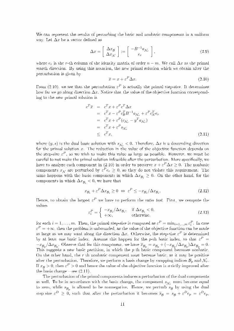
We can represent the results of perturbing the basic and nonbasic components in a uniformway. Let ∆x be a vector de�ned as

∆x =

[∆xB∆xN

]:=

[−B−1aNr

er

], (2.9)

where er is the r-th column of the identity matrix of order n−m. We call ∆x as the primalsearch direction. By using this notation, the new primal solution which we obtain after theperturbation is given by

x = x+ εP∆x. (2.10)

From (2.10), we see that the perturbation εP is actually the primal step-size. It determineshow far we go along direction ∆x. Notice that the value of the objective function correspond-ing to the new primal solution is

cTx = cTx+ εP cT∆x

= cTx− εP cTBB−1aNr+ εP cTN er

= cTx+ εP (cNr− yTaNr

)

= cTx+ εP sNr

≤ cTx, (2.11)

where (y, s) is the dual basic solution with sNr< 0. Therefore, ∆x is a descending direction

for the primal solution x. The reduction in the value of the objective function depends onthe step-size εP , so we wish to make this value as large as possible. However, we must becareful to not make the primal solution infeasible after the perturbation. More speci�cally, wehave to analyze each component in (2.10) in order to preserve x + εP∆x ≥ 0. The nonbasiccomponents xN are perturbed by εP er ≥ 0, so they do not violate this requirement. Thesame happens with the basic components in which ∆xBi ≥ 0. On the other hand, for thecomponents in which ∆xBi < 0, we have that

xBi + εP∆xBi ≥ 0 ⇔ εP ≤ −xBi/∆xBi , (2.12)

Hence, to obtain the largest εP we have to perform the ratio test. First, we compute thevalues

εPi =

{−xBi/∆xBi , if ∆xBi < 0,

+∞, otherwise.(2.13)

for each i = 1, . . . ,m. Then, the primal step-size is computed as εP = mini=1,...,m εPi . In case

εP = +∞, then the problem is unbounded, as the value of the objective function can be madeas large as we may want along the direction ∆x. Otherwise, the step-size εP is determinedby at least one basic index. Assume this happen for the p-th basic index, so that εP =−xBp/∆xBp . Observe that for this component, we have xBp = xBp + (−xBp/∆xBp)∆xBp = 0.This suggests a new basic partition, in which the p-th basic component becomes nonbasic.On the other hand, the r-th nonbasic component must become basic, as it may be positiveafter the perturbation. Therefore, we perform a basis change by swapping indices Bp and Nr.If xB > 0, then εP > 0 and hence the value of the objective function is strictly improved afterthe basis change � see (2.11).

The perturbation of the primal components induces a perturbation of the dual componentsas well. To be in accordance with the basis change, the component sNr

must become equalto zero, while sBp is allowed to be nonnegative. Hence, we perturb sB by using the dual

step-size εD ≥ 0, such that after the perturbation it becomes sB = sB + εDep = εDep,

11

where ep is the p-th column of the identity matrix of order m. Notice that only the p-th basiccomponent is perturbed. According to the dual general solution (2.6), this perturbation a�ectsthe components of y and the nonbasic components sN . Indeed, after adding the perturbationwe obtain

yT = cTBB−1 − εDeTpB−1

= yT + εD∆yT ,

where ∆y := −(eTpB−1)T = −(B−1)T ep. By using this result, the perturbation of the nonbasic

dual components leads to

sTN = cTN − (yT + εD∆yT )N (2.14)

= sTN − εD∆yTN

= sTN + εD∆sTN ,

where ∆sN := −(∆yTN)T = −NT∆y. If we further de�ne ∆sB := ep, then the new dualsolution we obtain after adding the perturbation is given by

(y, s) = (y, s) + εD(∆y,∆s). (2.15)

The dual step-size εD must be chosen in order to satisfy sNr= 0, as the index Nr was chosen

to enter the basis. Hence, we have that

sNr= 0 ⇔ sNr

+ εD∆sNr= 0 ⇔ εD = −sNr

/∆sNr.

This ratio is well-de�ned and leads to εD > 0, as we have sNr< 0 and ∆sNr

> 0. Indeed sNr

is the infeasible component of the nonbasic dual solution which motivates the perturbation ofthe primal solution � see (2.7). In addition, we have that

∆sNr= ∆sTN er

= −∆yTNer

= eTpB−1Ner

= eTpB−1aNr

= −eTp ∆xB

= −∆xBp . (2.16)

From the ratio test operation, we have ∆xBp < 0 and thus ∆sNr> 0. Therefore, even when

the primal step-size εP is equal to zero, then the dual step-size εD is strictly larger than zero.In summary, we have de�ned the search direction (∆x,∆y,∆s) and the step-sizes εP and

εD which will be used to obtain new primal and dual solutions. The new solutions suggest abasis change, in which the current r-th nonbasic index becomes basic, and the current p-thbasic index becomes nonbasic. If εP > 0, then the value of the objective function is strictlyreduced after the basis change. Otherwise, the value remains the same (but it never becomesworse). The basis change that we described determines a single iteration of the primal simplexmethod.

Algorithm 2 presents the primal simplex method for problems in the standard form. Theparameter IT_MAX sets the maximum number of iterations. In line 7, the algorithm checksthe optimality conditions (2.2). Only the nonbasic components of the dual solution s canviolate the optimality conditions. In case they are feasible, then the current primal basic

12

solution is optimal and the algorithm terminates. Otherwise, the pricing operation selects aninfeasible component sNr

. If more than one component is infeasible, then we follow a givenrule to select one of them. Several pricing rules are proposed in the literature. For instance,in the Dantzig's rule we select the index which corresponds to the minimum sNi

< 0 (ties canbe broken arbitrarily). See Maros (2003a) for a review of the pricing rules that are the mostused in practice.

Algorithm 2: Primal simplex method for problems in the standard form.Input: matrix A; parameters c and b; basic partition A = [B | N ] which is primal feasible; IT_MAX.Output: optimal solution x; or it detects the problem is unbounded; or IT reaches IT_MAX.

1 IT = 0;2 Compute the primal basic solution: xB := B−1b and xN := 0;3 Compute the dual basic solution: y := cTBB

−1, sB := 0 and sN := cN −NT y;4

5 While (IT < IT_MAX) do6 {7 If (sN ≥ 0) then STOP, an optimal solution has been found ;8 Pricing operation: choose an index r such that sNr

< 0;9 Compute the primal search direction: ∆xB := −B−1aNr

and ∆xN := er;10

11 Set p := −1;12 Ratio test: p := arg mini=1,...,n{−xBi

/∆xBi| ∆xBi

< 0};13 If (p = −1) then STOP, the problem is unbounded ;14 Compute the primal step-size: εP = −xBp

/∆xBp;

15

16 Compute the dual search direction: ∆y := −(B−1)T ep, ∆sB := ep and ∆sN := −NT ∆y;17 Compute the dual step-size: εD = −sNr

/∆sNr;

18

19 Update the current solution: (x, y, s) := (x, y, s) + (εP ∆x, εD∆y, εD∆s);20 Basis change: Nr becomes the p-th basic index and Bp becomes the r-th nonbasic index;21 IT = IT + 1;22 }

Notice that Algorithm 2 requires as input a partition which is primal feasible. In practice,this information may be di�cult to known in advance. In such case, a phase-1 algorithmmay be called before Algorithm 2 in order to obtain a basic feasible solution (Maros, 1986).Alternatively, we can recur to the big-M strategy, which inserts arti�cial variables to theproblem (Bertsimas and Tsitsiklis, 1997). It is worth mentioning that in order to have asuccessful implementation of Algorithm 2, it is important to rely on appropriate computationaltechniques. For a review on the main techniques we suggest the publications by Maros (2003a)and Munari (2009).

2.2.3 Dual simplex method

Given the linear programming problem (P ) in (2.1), consider a basic partition A = [B | N ]of the coe�cient matrix, such that the corresponding dual basic solution (y, s) is feasible.Assume that the primal basic solution x is not feasible and, hence, it cannot be optimal. Wepropose to obtain a new basic solution by using the dual simplex strategy, which consistsin perturbing a basic component of the dual solution. Since the perturbed component maybecome positive, the resulting dual solution suggests a basis change.

Assume that the primal basic solution x has a basic component xBp < 0 and hence itis infeasible. We propose to perturb the corresponding dual component by making sBp =

13

sBp + εD = εD, where εD is a given perturbation. The remaining basic components are keptat zero, so that we have

sB = sB + εD∆sB, (2.17)

where ∆sB := ep and ep is the p-th column of the identity matrix of order m. From thegeneral solution (2.6), we see that this perturbation results in modifying the components ofthe dual solution y as follows

yT = cTBB−1 − εDeTpB−1

= yT + εD∆yT ,

where ∆y := −(B−1)T ep, exactly as we have de�ned in the previous section. Furthermore,the nonbasic components become

sTN = cTN − (y + εD∆y)TN

= sTN − εD∆yTN

= sTN + εD∆sTN , (2.18)

where ∆sN := −NT∆y, which follows the same de�nition as in the previous section as well.Hence, the perturbation of the dual solution is given by (y, s) = (y, s)+εD(∆y,∆s),. From thisexpression, we see that εD is the step-size we adopt along the dual direction (∆y,∆s). Noticethat the value of the objective function which corresponds to the perturbed dual solution isgiven by

bT y = bT (y + εD∆y)

= bT y − εDbT (B−1)T ep

= bT y − εD(B−1b)T ep

= bT y − εDxBp .

Therefore, we see that the objective function changes by the amount −εDxBp > 0 in relation

to its previous value. Since xBp is strictly smaller than zero, a step-size εD > 0 results instrictly improving the value of the objective function. The change in this value is proportionalto εD, so we should set this step-size as large as possible. On the other hand, we want tokeep the dual solution feasible after the perturbation. In particular, we must guarantee thatsN ≥ 0. The other dual components remain feasible, as sBp is the only basic component we

perturb, and y is a free variable. Observe in (2.18) that only the negative components of ∆sNmay cause sN to become infeasible. In particular for such components, we must guaranteethat sNi

+ εD∆sNi≥ 0, which leads to

εD ≤ −sNi/∆sNi

. (2.19)

This suggests a ratio test in which we compute the ratio in (2.19) for each nonbasic indexand, then, we set εD as the smallest ratio. This leads to the largest step-size such that thenew dual solution (y, s) is feasible. Formally, we compute εD = mini=1,...,n−m = εDi , where

εDi =

{−sNi

/∆sNi, if ∆sNi

< 0,

+∞, otherwise.(2.20)

If we obtain εD = +∞ after performing the ratio test, then the dual problem (D) is unboundedand, thus, the primal problem (P ) is infeasible. Otherwise, we have εD = εDr for at least one

14

index r, r = 1, . . . , n − m (in case of ties, we can break them arbitrarily). Notice that byusing this step-size we obtain

sNr= sNr

+ εD∆sNr= sNr

+

(−

sNr

∆sNr

)∆sNr

= 0.

On the other hand, recall that the p-th basic component becomes sBp = εD = −sNr/∆sNr

.This suggests a basis change, in which the p-th basic index becomes nonbasic and the r-thnonbasic index becomes basic. Associated to this new basis, we have the basic dual solution(y, s) = (y, s)+εD(∆y,∆s), where the dual step-size εD and the dual search direction (∆y,∆s)were de�ned above.

The primal solution x must be perturbed as well in order to re�ect the basis change. Byusing the perturbation εP ≥ 0, we perturb the r-th nonbasic component only, i.e.,

xN = xN + εP er = εP∆xN ,

where ∆xN := er and er is the unitary vector which corresponds to the r-th column of theidentity matrix of order n−m. According the primal general solution (2.4), this perturbationmodi�es the basic components as follows

xB = B−1b− εPB−1Ner = xB + εP∆xB,

where ∆xB := −B−1Ner = −B−1aNr. Hence, ∆x = (∆xB,∆xN ) is the primal search

direction, as de�ned in (2.9). In addition, the perturbation εP corresponds to the primal step-size that we take along direction ∆x. To compute εP , we take into account the assumptionthat the index Bp becomes nonbasic after the basis change. Hence, we must have xBp = 0,which implies in

εP = −xBp

∆xBp.

This ratio is well-de�ned, since ∆xBp = −∆sNr> 0 (see (2.16)). In addition, we have εP > 0

as xBp < 0 is the infeasible primal component which motivates the perturbation in (2.17).The discussion presented so far describes the key ideas of the dual simplex method. This

method starts with a basis which is dual feasible, but primal infeasible. At each iteration,the method checks if the current basic solution is optimal by verifying the feasibility of theprimal solution. If the primal solution is also feasible, then it is an optimum of problem (P) in(2.1), as the dual solution is feasible at any iteration. Otherwise, a basis change is performedin order to obtain a new basis. Algorithm 3 presents the dual simplex method for problemsin the standard form. It is very similar to the primal simplex method given in Algorithm 2.The main di�erence is in the choice of the variables that will be swapped in the basis change.Indeed, the primal method select �rst the index that will enter the basis, and then determineswhich index will leave the basis. On the other hand, in the dual method the index that willleave the basis is selected �rst.

In Algorithm 3, we assume that a basic partition with a feasible dual basic solution is givenas an input. In case a basic partition with such feature is not known in advance, a dual phase-1method should be called before calling Algorithm 3. Di�erent types of dual phase-1 methodsare proposed in the literature (Kostina, 2002; Koberstein and Suhl, 2007). Alternatively, wecan use the big-M approach, although it typically causes the numerical instability of thesimplex method (Bertsimas and Tsitsiklis, 1997; Koberstein and Suhl, 2007). An e�cientand stable implementation of Algorithm 3 requires the use of appropriate computationaltechniques, which is out of the scope of this chapter. For the reader interested in thesetechniques we suggest the publications by Maros (2003a) and Koberstein (2005).

15

Algorithm 3: Dual simplex method for problems in the standard form.Input: matrix A; parameters c and b; basic partition A = [B | N ] which is dual feasible; IT_MAX.Output: optimal solution x; or it detects the problem is infeasible; or IT reaches IT_MAX.

1 IT = 0;2 Compute the primal basic solution: xB := B−1b and xN := 0;3 Compute the dual basic solution: y := cTBB

−1, sB := 0 and sN := cN −NT y;4

5 While (IT < IT_MAX) do6 {7 If (xB ≥ 0) then STOP, an optimal solution has been found ;8 Pricing operation: choose an index p such that xBp

< 0;

9 Compute the dual search direction: ∆y := −(B−1)T ep, ∆sB := ep and ∆sN := −NT ∆y;10

11 Set p := −1;12 Ratio test: r := arg mini=1,...,n−m{−sNi

/∆sNi| ∆sNi

< 0};13 If (p = −1) then STOP, the problem is infeasible;14 Compute the dual step-size: εD = −sNr

/∆sNr;

15

16 Compute the primal search direction: ∆xB := −B−1aNrand ∆xN := er;

17 Compute the primal step-size: εP = −xBp/∆xBp

;

18

19 Update the current solution: (x, y, s) := (x, y, s) + (εP ∆x, εD∆y, εD∆s);20 Basis change: Nr becomes the p-th basic index and Bp becomes the r-th nonbasic index;21 IT = IT + 1;22 }

2.3 The primal-dual interior point method

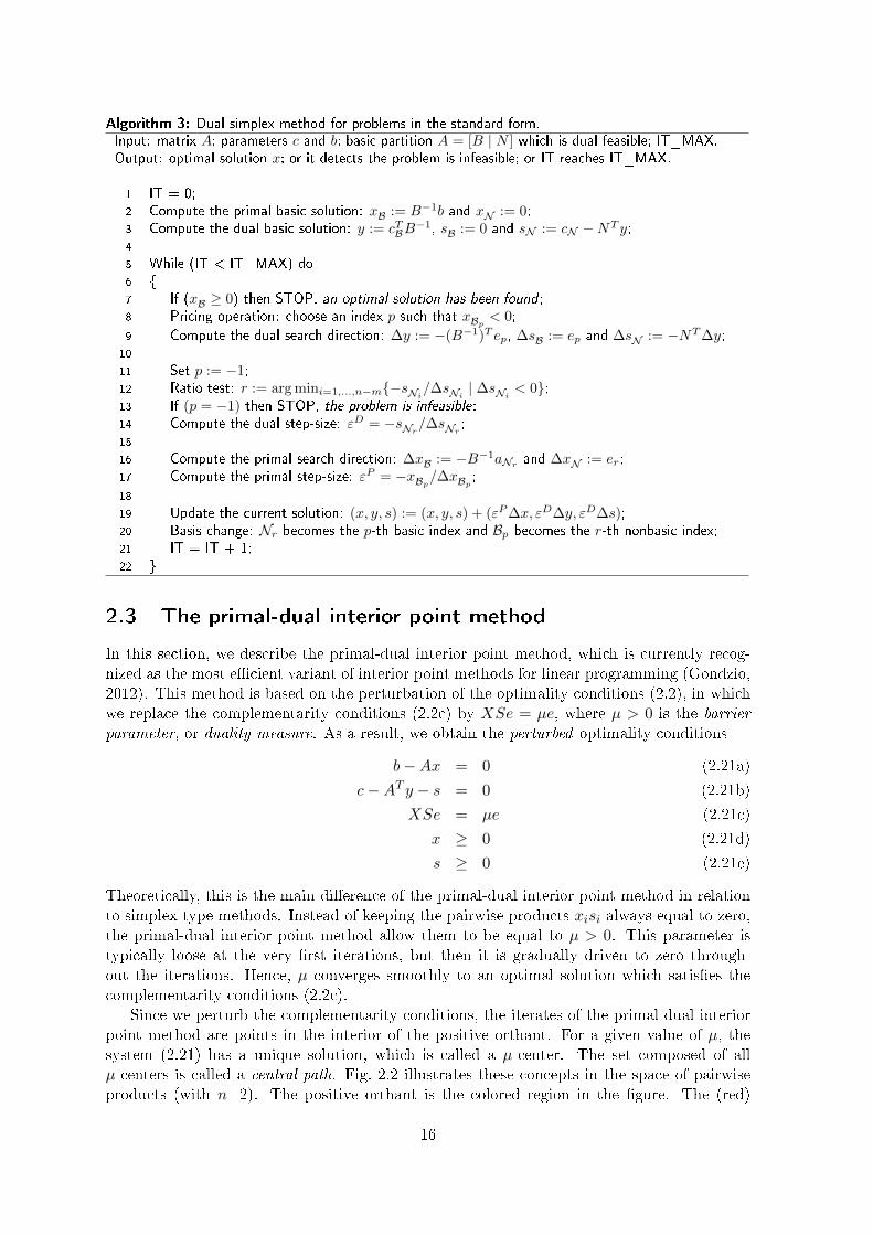
In this section, we describe the primal-dual interior point method, which is currently recog-nized as the most e�cient variant of interior point methods for linear programming (Gondzio,2012). This method is based on the perturbation of the optimality conditions (2.2), in whichwe replace the complementarity conditions (2.2c) by XSe = µe, where µ > 0 is the barrier

parameter, or duality measure. As a result, we obtain the perturbed optimality conditions

b−Ax = 0 (2.21a)

c−AT y − s = 0 (2.21b)

XSe = µe (2.21c)

x ≥ 0 (2.21d)

s ≥ 0 (2.21e)

Theoretically, this is the main di�erence of the primal-dual interior point method in relationto simplex type methods. Instead of keeping the pairwise products xisi always equal to zero,the primal-dual interior point method allow them to be equal to µ > 0. This parameter istypically loose at the very �rst iterations, but then it is gradually driven to zero through-out the iterations. Hence, µ converges smoothly to an optimal solution which satis�es thecomplementarity conditions (2.2c).

Since we perturb the complementarity conditions, the iterates of the primal-dual interiorpoint method are points in the interior of the positive orthant. For a given value of µ, thesystem (2.21) has a unique solution, which is called a µ-center. The set composed of allµ-centers is called a central-path. Fig. 2.2 illustrates these concepts in the space of pairwiseproducts (with n=2). The positive orthant is the colored region in the �gure. The (red)

16

dashed lines represent the set of points which satisfy the complementarity conditions (2.2c).The continuous line in the middle of the positive orthant represents the central path. For agiven a value µ > 0, the µ-center is a point in the central path that satis�es x1s1 = x2s2 = µ.

x2 s2

x1 s1

k p

k

k p k x1 s1

x2 s2

x1 s1

x2 s2

k

k

kp

x2 s2

x1 s1

x1 s1

x2 s2

k 1

k k p 1

k p

k p

1

k p

k

1

k

x2 s2

1

k

1

k x1 s1

k

k

μ

μ

μk

μk+ p

μk

μk+ p

μk

μk

x1 s1=x2 s2=μ

Central path

x1 s1=0

x2 s2=0

Figure 2.2: Illustration of the positive orthant in the space of pairwise products, with n = 2.

Instead of strictly satisfying the perturbed optimality conditions, the iterates of the primal-dual interior point method belong to a neighborhood of the central path. The idea of theneighborhood is to keep the iterates well-centered and in a safe area so that all variablesapproach their optimal values with a uniform pace. Di�erent neighborhoods have been pro-posed in the literature, and they di�er by the way they measure the distance of the pairwiseproducts xisi to the duality measure µ. For instance, the narrow neighborhood is de�ned as

N2(θ) = {(x, y, s) ∈ F0 | ‖XSe− µe‖2 ≤ θµ},

where F0 = {(x, y, s) | Ax = b, AT y + s = c and (x, s) > 0} is the set of positive primal-dualfeasible solutions, and θ ∈ [0, 1) is a given parameter. The set of pairwise products thatsatisfy the inequality imposed by N2(θ) is illustrated in Fig. 2.3 for iterates k and k + p, forany given k > 0 and p > 0. The continuous line inside the positive orthant represents thecentral path. The (black) points in the central path are the µ-centers corresponding to theduality measures µk and µk+p. We can de�ne a neighborhood by using the ∞-norm as well.By adopting only the lower bound on xisi, we obtain the wide neighbourhood, which is de�nedas

N−∞(γ) = {(x, y, s) ∈ F0 | xisi ≥ γµ,∀i = 1, . . . , n},

where γ ∈ (0, 1) is a �xed parameter. Notice that this neighborhood is less restrictive thanN2(θ). An illustration of the N−∞(γ) in the set of pairwise products is given in Fig. 2.4. Inthe wide neighborhood, if we further impose upper bounds on the pairwise products, then weobtain the symmetric neighborhood, which is de�ne as

Ns(γ) = {(x, y, s) ∈ F0 | γµ ≤ xisi ≤1

γµ, ∀i = 1, . . . , n},

with γ ∈ (0, 1). This neighborhood is illustrated in Fig. 2.5. The choice of the neighborhooda�ects the theoretical as well as practical properties of the algorithm. If the primal-dual

17

x2 s2

x1 s1γμ

k

γμk

k p

k

k p k x1 s1

x2 s2

x1 s1

x2 s2

k

k

kp

x2 s2

x1 s1

x1 s1

x2 s2

k 1

k k p 1

k p

k p

1

k p

k

1

k

x2 s2

1

k

1

k x1 s1

k

k

μk

μk

μk

μk+ p

μk

μk+ p

μk

μk

μk

μk+ p

μk

μk

μk+ p

Figure 2.3: Narrow neighborhood in the space of pairwise products with the duality mea-sures of iterations k and k+p (the set F0 is not represented in the illustration).

x2 s2

x1 s1γμ

k

γμk

k p

k

k p k x1 s1

x2 s2

x1 s1

x2 s2

k

k

kp

x2 s2

x1 s1

x1 s1

x2 s2

k 1

k k p 1

k p

k p

1

k p

k

1

k

x2 s2

1

k

1

k x1 s1

k

k

μk

μk

μk

μk+ p

μk

μk+ p

μk

μk

μk

μk+ p

μk

μk

μk+ p

Figure 2.4: Wide neighborhood in the space of pairwise products with the duality measuresof iterations k and k + p (the set F0 is not represented in the illustration).

x2 s2

x1 s1γμ

k

γμk

k p

k

k p k x1 s1

x2 s2

x1 s1

x2 s2

k

k

kp

x2 s2

x1 s1

x1 s1

x2 s2

k 1

k k p 1

k p

k p

1

k p

k

1

k

x2 s2

1

k

1

k x1 s1

k

k

μk

μk

μk

μk+ p

μk

μk+ p

μk

μk

μk

μk+ p

μk

μk

μk+ p

Figure 2.5: Symmetric neighborhood in the space of pairwise products with the duality mea-sures of iterations k and k+p (the set F0 is not represented in the illustration).

18

interior point algorithm is based on the narrow neighborhood N2, then it achieves a solutionthat satis�es µ < ε in O(

√n| log(1/ε)|) iterations, by starting from a solution that satis�es µ ≤

1/εκ, for some positive κ. By using the wide neighborhood N−∞, the worst-case complexityof the method is a bit worse, given by O(n| log(1/ε)|) iterations. In spite of this, the practicalperformance of the method that uses the N−∞ is typically superior to the method using theN2. The theoretical and practical features of the symmetric neighborhood is similar to thatof the wide neighborhood, but it is preferred by some authors (Colombo and Gondzio, 2008;Gondzio, 2012).

The description of the primal-dual interior point algorithm follows the linear programmingframework de�ned by Algorithm 1. At each iteration, given an iterate (x, y, s), we computethe primal-dual search direction (∆x,∆y,∆s) and the primal and dual step-sizes, εP and εD,so that the next iterate is given by

(x, y, s) = (x, y, s) + (εP∆x, εD∆y, εD∆s).

The search direction (∆x,∆y,∆s) is obtained by solving the Newton step equations A 0 00 AT IS 0 X

∆x∆y∆s

=

00

σµe−XSe

, (2.22)

where σ ∈ [0, 1] is a parameter used to reduce the complementarity gap xT s of the nextiterate. For σ = 0, the system of equations (2.22) corresponds to a �rst order approximationof the perturbed optimality conditions (2.21). We obtain this approximation by applyingone step of the Newton method. The solution with σ = 0 is the a�ne-scaling direction,which corresponds to the usual direction of the Newton method. On the other hand, σ = 1determines a centering direction toward a µ-center in the central path, which has all thepairwise products identical to µ. Hence, by setting an intermediate value for σ we obtaina combination of these two extreme directions. The resulting direction contributes to bothoptimality and centrality. After obtaining the primal-dual search direction, the step-sizes εP

and εD are computed by performing a line search along the direction (∆x,∆y,∆s). Thechosen step-sizes must guarantee that the next iterate belongs to the used neighborhood.

Following the discussion that we have presented so far, the primal-dual interior pointmethod is stated in Algorithm 4. In the algorithm, we denote by N? a neighborhood of thecentral path, which can be any of those described above. In line 7, the algorithm obtainsthe primal-dual search direction by solving the Newton step equations (2.22). In practice,we reformulate this system of equations in order to obtain a more compact coe�cient matrixwhich is in addition symmetric. The idea is to obtain a more e�cient representation ofthe matrix, which contributes to a better overall performance of the method. Two types ofreformulations are used in practice, depending on the structure of the coe�cient matrix of(2.22). They are known as the augmented system and the normal equations. Recall that x ands are positive at any iteration of the primal-dual interior point algorithm, so the matrices Xand S are nonsingular. The augmented system consists in eliminating ∆s from step equations,so that we obtain [

0 AAT −D−2

] [∆y∆x

]=

[0

s− σµX−1e

], (2.23)

∆s = −s+ σµX−1e−X−1S∆x,

where D := S−12X

12 . In the normal equations, we go a step further and eliminate ∆x from

(2.23) and, hence, we obtain

AD2AT∆y = A(x− σµS−1e), (2.24)

19

∆s = −AT∆y,

∆x = −x+ σµS−1e− S−1X∆s.

The normal equations are widely used in practice. The coe�cient matrix in (2.24) is symmetricpositive semide�nite. Hence, this matrix is represented by the Cholesky factorization, whichis very e�cient in practice. It requires appropriate techniques to avoid numerical instabilitiescaused by small components of x and s, which typically appears in the very last iterations.The coe�cient matrix in (2.23) is symmetric inde�nite, which makes its factorization morecomplicated than in the normal equations. Nevertheless, the augmented system is moree�cient when the matrix A has one or more dense columns, which justi�es its use.

Algorithm 4: Primal-dual interior point method for problems in the standard form.Input: matrix A; parameters c and b; barrier reduction parameter σ ∈ (0, 1); IT_MAX;

primal-dual feasible solution (x, y, s) ∈ N?.Output: optimal solution x?; or IT = IT_MAX.

1 IT = 0;2 Set the barrier parameter: µ := (xT s)/n;3 While (IT < IT_MAX) do4 {5 If the optimality conditions (2.2) are satis�ed then STOP, an optimal solution has been found ;6 Reduce the barrier parameter: µ := σµ;7 Compute the primal-dual search direction (∆x,∆y,∆s) by solving the Newton step equations;8

9 Find εP and εD as the largest step-sizes such that (x+ εP ∆x, y + εD∆y, s+ εD∆s) ∈ N?;10 Reset the step-sizes: εP := 0.99εP and εD := 0.99εD;11

12 Update the solution: (x, y, s) := (x, y, s) + (εP ∆x, εD∆y, εD∆s);13 }

Algorithm 4 requires the initial solution to belong to a given neighborhood. Hence, theinitial solution must be primal and dual feasible, so the problem cannot be infeasible neitherunbounded. In practice, a solution with such feature may be di�cult to obtain. To overcomethis, we can recur to the infeasible primal-dual interior point method. This algorithm is verysimilar to Algorithm 4, but it relies in a relaxed neighborhood of the central path. Thisneighborhood does not require the iterates to satisfy the systems of constraints Ax = b andAT y + s = c, but only the positivity conditions (x, s) > 0. The method deals with theinfeasibilities by incorporating them to the right-hand side of the Newton step equations(2.22), i.e., A 0 0

0 AT IS 0 X

∆x∆y∆s

=

b−Axc−AT y − sσµe−XSe

. (2.25)

The modi�ed neighborhood simpli�es the line search which determines the primal and dualstep-sizes. Indeed, εP and εD are taken as the largest values such that x + εP∆x > 0 ands + εD∆s > 0. Therefore, the step-sizes are computed by using a ratio test, similar to thatused in simplex-type methods (see Algorithms 2 and 3). For further details on the infeasibleprimal-dual interior point algorithm, we suggest the paper by Gondzio (2012).

2.3.1 Warmstarting the primal-dual interior point algorithm

In this section, we address the reoptimization of a problem by using the primal-dual interiorpoint method. The reoptimization is important to situations in which closely-related problems

20

are solved in sequence. By closely-related problems we mean that the problems di�er bychanges such as inserting/dropping constraints and/or columns, �xing/relaxing variables, andperturbing the problem data. These situations arise, for example, in the context of the columngeneration method and of the branch-and-bound method. By using a warmstarting technique,we exploit some available information in order to de�ne an advanced initial point to start theprimal-dual interior point method. The goal is to improve the performance of solving theproblem in relation to starting from a standard initial point. In the next paragraphs, webrie�y describe the issues involved in the warmstarting operation. The purpose is to presentthe main ideas which are proposed in the literature. The theoretical and computational detailsof the warmstarting strategies is out of the scope of this chapter. They can be found in thereferences presented throughout the discussion.

It is well-known the ability of simplex-type methods to reoptimize similar problems froma previous optimal solution. Typically, by starting from the optimal basis of the previousproblem, a relatively small number of basis changes are enough to reach the optimal solutionof the new problem. In addition, the optimal basis of the previous problem is usually eitherprimal feasible or dual feasible to the new problem. Nevertheless, for interior point methods,the optimal solution of a closely-related problem is not a good initial point in general. Indeed,this solution is likely to be at or very close to the boundary of the primal-dual feasible set F0.In such case, the initial point is badly centered, so it leads to many iterations with very smallstep-sizes, which slow down the convergence of the method. In addition to be badly centered,the initial point may violate some primal or dual constraints as well, which is an issue forthe feasible primal-dual interior point method. Therefore, the reoptimization in interior pointmethods cannot be interpreted very literally as in simplex-type methods.

There are two main concerns regarding the warmstarting point in interior point methods.First, it should satisfy the primal and dual constraints. In case of the infeasible variant ofthe method, the infeasibility of the initial point should be small enough to be absorbed in the�rst iterations of the method. Second, the pairwise products must be positive and should notdeviate too much from each other. In other words, the iterates must be well-centered in thepositive orthant. These requirements are illustrated in Fig. 2.6, which shows di�erent typesof candidate initial points. Suitable initial points are represented by the (green) balls in the�gure. They are feasible as shown in part (a), and well-centered in the positive orthant, asshown in part (b). For the infeasible primal-dual interior point method, the point representedby a (yellow) triangle in part (a) should be suitable as well. The (red) squares in the �gurecorrespond to infeasible and/or badly centered points, so they are not suitable as initial points.

In the last 15 years, the research regarding e�cient warmstarting techniques for interiorpoint methods has been very active. We classify these techniques into two groups: (i) one-phase techniques; and (ii) two-phase techniques. In the one-phase techniques, the problemis modi�ed by the addition of slack variables and/or penalization factors so that the optimalsolution (x, y, s) of a closely-related problem is used as the initial point. The problem ismodi�ed in such a way that (x, y, s) is not too close to the boundary of the modi�ed feasibleset. Fig. 2.7 illustrates the idea of the one-phase techniques. Recall that in Fig. 2.6, severalcandidate initial points are available, but some of them were not good initial points in thespace of pairwise products. In the one-phase techniques we expand this space, by relaxingthe nonnegativity constraints, as illustrated in Fig. 2.7. As a result, all the points becomeacceptable initial points and can be used as a warmstarting point. Of course, the expandedboundaries must be driven to zero again during the solution of the problem. Warmstartingtechniques in this group have been proposed by Benson and Shanno (2007) and Engau et al.(2009, 2010). They di�er from each other by how the space of pairwise products is expanded.

21

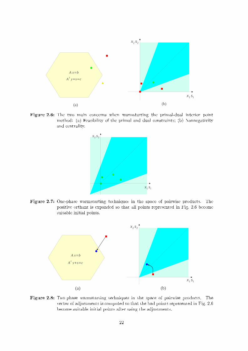
x1 s1

x1 s1

x2 s2

x2 s2

Warmstarting techniques

One-phase Two-phase

Phase 2:Solve the problem

x , y , z

x , y ,z

x x , y y ,z z

Phase 1:Compute the adjustmentSolve a modified problem

with artificial variables

The optimal solution mustbe an optimal solutionof the original problem

x , y ,z

,

A x=b

AT y+s=c

(b)

(a)

x1 s1

x1 s1

x2 s2

x2 s2


One-phase Two-phase


x , y , z

x , y ,z

x x , y y ,z z




x , y ,z

,

A x=b

AT y+s=c

(b)

(a)

Figure 2.6: The two main concerns when warmstarting the primal-dual interior pointmethod: (a) Feasibility of the primal and dual constraints; (b) Nonnegativityand centrality.

x1 s1

x1 s1

x2 s2

x2 s2


One-phase Two-phase


x , y , z

x , y ,z

x x , y y ,z z




x , y ,z

,

A x=b

AT y+s=c

(b)

(a)

Figure 2.7: One-phase warmstarting techniques in the space of pairwise products. Thepositive orthant is expanded so that all points represented in Fig. 2.6 becomesuitable initial points.

x2 s2

x1 s1

AT y+s=c

A x=b

(b)(a)

x2 s2

x1 s1

AT y+s=c

A x=b

(b)(a)

Figure 2.8: Two-phase warmstarting techniques in the space of pairwise products. Thevector of adjustments is computed so that the bad points represented in Fig. 2.6become suitable initial points after using the adjustments.

22

Two-phase techniques are characterized by modifying one or more stored points of aclosely-related problem. In the �rst phase, a stored point (x, y, s) is adjusted by a vector(∆x,∆y,∆s) so that it becomes feasible (or slightly infeasible) and better centered in thepositive orthant. The adjustment can be performed in a single step or by using an iterativeprocess in which several stored points are modi�ed through one or more adjustments. In thesecond phase, the adjusted point (x+ ∆x, y+ ∆y, s+ ∆s) is used as the initial point. Fig. 2.8illustrates the idea of the two-phase techniques. The arrows represent the adjustments whichare applied to the stored points. The adjusted points are represented by a (blue) ball in the�gure. The �rst two-phase warmstarting techniques for the primal-dual interior point methodwere proposed by Mitchell and Borchers (1996) and Gondzio (1998). Those papers have pro-posed the basic ideas which are used in the subsequent techniques proposed by Yildirim andWright (2002); Gondzio and Grothey (2003, 2008); John and Yildirim (2008).

To further clarify the main ideas of the warmstarting techniques, we close this section bybrie�y describing the strategy proposed by Gondzio (1998). This strategy is the basis of thewarmstarting procedures that are implemented in the interior point solver HOPDM (Gondzio,1995, 2012). This solver is used in the computational experiments presented in Chapters 4and 5 of this thesis. Gondzio's warmstarting technique was proposed for the case in whichnew columns are added to the problem after solving it. Nevertheless, the key ideas used inthis strategy have been successfully extended to other contexts Gondzio and Grothey (2003).

Consider a linear programming problem which is formulated as the primal problem (P)in (2.1). Assume that after solving this problem, we modify it by adding n > 0 columnsto its coe�cient matrix. We represent the new columns by a submatrix A. The variablescorresponding to these columns are represented by the vector w ∈ Rn. The changes in theprimal problem result in new constraints to the dual problem (D). The resulting primal-dualpair of problems is given by

(P ) min cTx+ cTw

s.t. Ax+ Aw = bx, w ≥ 0,

(D) max bT ys.t. AT y + s = c

AT y + z = cs, z ≥ 0.

(2.26)

We want to solve the primal problem (P ) in (2.26) by using some information from theclosely-related problem (P ) in (2.1). Gondzio (1998) proposes a warmstarting techniquewhich uses a close-to-optimality approximate µ-center which is stored during the solution ofthe closely-related problem. Since this point may violate the feasible set of the new problem(P ), the author suggests to compute an adjustment in order to modify the stored point. Theadjustment should generate a warmstarting point that is nearly feasible and relatively closeto the central path. As observed by the author, since we do not know the new columns inadvance, the choice of the µ-center is a safe option because it is the center of an ellipsoidinscribed in the dual feasible region. Hence, it is possible to take at least a small step fromthis point in order to correct the infeasibilities caused by the new columns.

To store the µ-center that will be used in a subsequent problem, the solution process needto be split into two stages. The interior point method iterates until the required tolerance εµof the µ-center is achieved (e.g., εµ = 0.001). Then, if the current iterate is not su�cientlywell-centered, a few additional centering steps are carried out in order to obtain a pointsatisfying

γµ ≤ xjsj ≤ (1/γ)µ,

for some γ > 0 (e.g., γ = 0.5). The resulting point is stored to be used in a subsequentproblem and the method continues iterating until the optimality tolerance is achieved. The

23

author recommends the use of centrality correctors (Gondzio, 1996; Colombo and Gondzio,2008) to e�ciently compute the centering steps.

Assume we have stored a µ-center (x, y, s) of the closely related problem (P ) in (2.1). Wewant to use this point to de�ne a warmstarting point (x, w, y, s, z) for solving the problem(P ) in (2.26), with (x, w) > 0 and (s, z) > 0. Let υ = c− AT y be the vector of n componentswhich corresponds to the depths of the new columns. We say that a column j is deep ifυj < −µ1/2. The components of the dual slack variable z are set as zj = max(

√µ, |υj |). The

choice w = 0 would lead to primal feasibility, but we need w > 0. By setting w = µZ−1ewe have that the new pairwise products are equal to the former barrier parameter µ, i.e.,W Ze = µe. To obtain suitable values for the variables x, y and s, we use the adjustmentvector (∆x,∆y,∆s). We compute the primal and the dual adjustments independently. Theprimal adjustment is given by

∆x = −D2AT (AD2AT )−1Aw.

Then, we compute a step-size αP such that (x+αP∆x, αP w) is feasible. For the dual variables,the adjustments are given by

∆y = (AD2AT )−1A(AT (AD2AT )−1A)−1υ,

∆s = −AT∆y.

A full step towards this direction in the dual space restores the feasibility of the new dualconstraints. However, this step-size may not be possible as ∆s depends on υ, which may belarge so s may become zero or negative. Thus, we compute the maximum step length αD sothat the dual variables are still positive after the adjustment. Therefore, the resulting pointis given by

(x, w, y, s, z) = (x+ αP∆x, αP w, y + αD∆y, s+ αD∆s, αDz),

which is used as the warmstarting point to solve problem (P ) in (2.26). This point can beslightly infeasible, but the remaining primal-dual infeasibilities will be removed during theoptimization if we use the infeasible primal-dual interior point method.

2.4 Concluding remarks

In this chapter, we have described the main linear programming methodologies, namely theprimal simplex method, the dual simplex method and the primal-dual interior point method.These methods are addressed in the remaining chapters of this thesis, and we follow the samenotation and nomenclature that was stated here. We have presented the methods by using auni�ed linear programming framework. This allows us to see what are the di�erences as well asthe similarities regarding these methodologies. In addition, we have presented the main issuesregarding the warmstarting of the primal-dual interior point method, as the methodologiesproposed in Chapters 4 and 5 depends on e�cient warmstarting techniques to work well inpractice.

24

Chapter 3

A dual simplex-type algorithm for

problems in the general form

Simplex-type methods are widely used nowadays. This class of methods was recognized asone of the ten most in�uential algorithms on science and engineering in the 20th century(Dongarra and Sullivan, 2000). In addition, Elwes (2012) states that the simplex method is�the algorithm that runs the world�. According to the author, implementations of simplex-type methods are called upon thousands of times a second over the world, in order to solveproblems related to our day-to-day lives. As a consequence, the search for more e�cientvariants of the simplex method has the potential to bene�t many di�erent areas.

In the last years, the researches regarding simplex-type methods have focused on di�erentbranches. For instance, the papers by Hall and McKinnon (2005), Koberstein (2008) and Huand Pan (2008) are mainly concerned with e�cient techniques that can be used to speed-up thecomputational implementations of the method. Maros (2003b), Paparrizos et al. (2003) andPan (2008) propose new variants of simplex-type methods, which exploit di�erent strategiesfor selecting the variables that enter/leave the basis. Recently, the community has raisedagain its attention to the theoretical complexity of the simplex method, due to a paper bySantos (2012) in which the author disprove the Hirsch conjecture (see e.g. Dantzig and Thapa,1997). Further theoretical breakthroughs were presented by Friedmann (2011) and Friedmannet al. (2011). The authors prove the exponential complexity of two nonstandard pivot rulesthat behave very well in practice.

In this chapter, we address a variant of the dual simplex method, in which we exploitspecial features of a type of formulation. In particular, we exploit the general form, a for-mulation in which all the constraints are represented as inequalities with lower and upperbounds, including the nonnegativity of the decision variables. As it will be seen, this for-mulation leads to a piecewise linear objective function in the dual problem. We exploit thisfeature to modify the choice of the dual step-size, in order to obtain larger steps. Besides, theproposed modi�cation helps to get rid of degenerate basic solutions.

It is worth mentioning that many solvers allow the user to enter with a linear programmingproblem in the general form. However, before calling the simplex method, they �rst transformthe general form to the standard form presented in Chapter 2, by adding slack and/or surplusvariables. What we propose in this chapter is the opposite strategy. The simplex method isdesigned in order to solve the problem in the general form, without the need to transformthe formulation. The reason is that the general form can be exploited in order to improvethe performance of the dual simplex method. In addition, we discard the need to add slackand surplus variables to the formulation. Another interesting feature is that we can insert

25

a new constraint lj ≤ ajx ≤ uj without changing the dimension of the basic matrix. Thisis important when the simplex method is used to solve a sequence of closely-related linearrelaxations, a common scenario when it is applied within an integer programming method-ology. For instance, a new constraint of this type may be generated after branching in thebranch-and-bound method, or after adding a cut in the cutting plane method.

In the remainder of this chapter, we address the dual simplex method for problems in thegeneral form. This study extends the earlier investigations regarding this method, which werepresented by Arenales (1984), Sousa et al. (2005) and Silva et al. (2007). In particular, themain contributions are:

• We describe how to explicitly handle bounds that are equal to −∞ or +∞ (Section3.1). Hence, we avoid the need for arti�cial bounds, which are known to cause numericalinstability of the method.

• To have a successful implementation of the method, it is essential to use e�cient tech-niques to represent and update the basic matrix. Hence, we describe how to extendthe LU factorization and LU update schemes proposed by Suhl and Suhl (1990, 1993)to the particular case we are dealing with (Section 3.6.2). These techniques are knownto be more e�cient than those used in the computational implementations of Sousaet al. (2005) and Silva et al. (2007). They typically reduce the �ll-in of the sparserepresentation of the basic matrix, and improve the numerical stability of the method.

• We show how to update the primal and dual solutions after carrying out a basis change,in order to avoid recomputing them from scratch at each iteration (Propositions 3.3.3and 3.5.2).

• The performance of the method is veri�ed by computational experiments using bench-marking instances from the public repository Netlib (Section 3.7). We compare themethod against other simplex-type variants.

Apart from the importance of simplex-type methods and the active research regardingthem, there is still a large gap between the techniques which are described in the literatureand those which are implemented by commercial solvers. In other words, many theoreticaland computational developments which are used to speed up the commercial implementationsof the simplex-type methods are not reported in the literature. As a consequence, the authorsare often discouraged in testing new strategies, as the computational performance of theirimplementations may be far from that of commercial solvers. With the investigation addressedin this paper, we hope to contribute with the literature by proposing a new theoretical andcomputational study regarding the dual simplex algorithm.

3.1 General form

Typically, we can model a linear programming problem by using di�erent types of formu-lations. This freedom in representing a problem allows us to choose the formulation thatmost suits our needs. For instance, a given formulation may be easier to be understood in atextbook, while another leads to a better performance of the solver. Here, we consider that alinear programming problem is formulated in the following general form:

min f(x) = cTx (3.1a)

s.t. l ≤ Ax ≤ u, (3.1b)

26

where A is a real matrix m × n with 0 < n ≤ m and rank(A) = n. The i-th column of Ais denoted by the vector ai ∈ Rm, while the j-th row of this matrix is denoted by aj ∈ Rn,with i ∈ I := {1, . . . , n} and j ∈ J := {1, . . . ,m}. The vectors c ∈ Rn, l ∈ Rm ∪ {−∞} andu ∈ Rm ∪ {+∞} are parameters of the problem, while x ∈ Rn is the vector of variables. Thecomponent ci is the cost associated to variable xi, for each i ∈ I. For each j ∈ J , a lowerbound lj and an upper bound uj is de�ned for the j-th constraint. Notice that these boundscan be real values as well as −∞ or +∞. As a consequence, we are able to represent anytype of linear constraint with this formulation. For instance, the equality ajx = bj for a givenbj ∈ R can be represented by lj ≤ ajx ≤ uj with lj = uj = bj . In addition, a nonnegativevariable can be represented by the constraint lj ≤ xj ≤ uj with lj = 0 and uj = +∞.

We classify the constraints in (3.1b) according to the respective components of bounds land u. Consider the following partition of set J :

J b = {j ∈ J | lj ∈ R and uj ∈ R},J l = {j ∈ J | lj ∈ R and uj = +∞},J u = {j ∈ J | lj = −∞ and uj ∈ R},J f = {j ∈ J | lj = −∞ and uj = +∞}.

Since it is a partition, we have J b∪J l∪J u∪J f = J and J b∩J l∩J u∩J f = ∅. A constraintin J b is called boxed. If in addition lj = uj , then we have a �xed constraint. Constraints insets J l and J u must have only one �nite bound. Finally, free constraints belong to set J f .Strictly speaking, they are not constraints, but we extend the nomenclature in order to followa standard presentation.

We can obtain a dual formulation for the general form (3.1). For the sake of clarity, weobtain this dual by using an equivalent formulation of (3.1), given by

min f(x) = cTx (3.2a)

s.t. Ax = w, (3.2b)

l ≤ w ≤ u. (3.2c)

The vector w is used to represent the constraints in (3.1b). The nomenclature of each con-straint according to the partition of J is extended to the corresponding component of w.From formulation (3.2), we de�ne the associated lagrangian problem:

h(y) := minx,w{cTx+ yT (w −Ax) | l ≤ w ≤ u} (3.3a)

= minx,w{(cT − yTA)x+ yTw | l ≤ w ≤ u} (3.3b)

= minx

(cT − yTA)x+ minw{yTw | l ≤ w ≤ u} (3.3c)

where the components of y ∈ Rm are the Lagrange multipliers. For any y and any x, h(y)gives a lower bound for f(x). Indeed, we have

f(x) ≥ minx,w{cTx | Ax = w, l ≤ w ≤ u}

= minx,w{cTx+ yT (w −Ax) | Ax = w, l ≤ w ≤ u}

≥ minx,w{cTx+ yT (w −Ax) | l ≤ w ≤ u}

= h(y)

27

Di�erent values of y may lead to di�erent lower bounds of f(x) and, hence, we are interestedin obtaining the best among them. The largest lower bound can be obtained by solving the(lagrangian) dual problem

maxh(y), y ∈ Rm. (3.4)

The representation of this problem can be improved by taking advantage of special cases inthe de�nition of the lagrangian problem (3.3). In particular, we add new constraints to (3.3)in order to avoid h(y)→ −∞. First, observe that x is free and thus for any y ∈ R we have

minx

(cT − yTA)x→ −∞, (3.5)

whenever cT − yTA 6= 0. To avoid this, we restrict the domain of the Lagrange multipliers byimposing cT − yTA = 0. In other words, we additionally require y ∈ D := {y ∈ Rm | yTA =cT } in (3.3). For the second term in expression (3.3c), notice that

minw

{yTw | l ≤ w ≤ u

}= min

w

∑j∈J

yjwj | lj ≤ wj ≤ uj , j ∈ J

=

∑j∈J

minwj

{yjwj | lj ≤ wj ≤ uj}

=∑j∈Jyj>0

yjlj +∑j∈Jyj<0

yjuj , (3.6)

as the variables wj are independent of each other. For each j ∈ J , let hj(yj) be a piecewiselinear function which is de�ned as follows

hj(yj) :=

ljyj , if yj > 0,ujyj , if yj < 0,0, otherwise.

(3.7)

Using this de�nition together with (3.3), (3.6) and the de�nition of D given above, we obtain

h(y) =∑j∈J

hj(yj).

Since the components lj and uj may be −∞ or ∞ , we may have hj(yj) equal to −∞ or +∞for a given j ∈ J . To avoid this undesirable situation, we further restrict the domain of theLagrange multipliers by requiring: yj ≤ 0, if lj = −∞ and uj ∈ R; yj ≥ 0, if lj ∈ R anduj =∞; and yj = 0, if lj = −∞ and uj =∞. In other words, we rede�ne D as

D := {y ∈ Rm | yTA = cT , yJ u ≤ 0, yJ l ≥ 0, yJ f = 0}.

If we incorporate all these changes to (3.4), the dual problem is given by

max h(y) =∑j∈J

hj(yj) (3.8a)

s.t. AT y = c, (3.8b)

yj ≤ 0, j ∈ J u, (3.8c)

yj ≥ 0, j ∈ J l, (3.8d)

yj = 0, j ∈ J f . (3.8e)

28

Observe that each hj(yj) is a (concave) continuous piecewise linear function. If lj 6= uj ,then it has a nondi�erentiable point (breakpoint) at yj = 0. Fig. 3.1 illustrates di�erent plotsthat the function hj(yj) may assume according to the bounds lj and uj . In part (a), j ∈ J band hence both bounds are �nite. The slope of function hj(yj) is lj > 0 for yj > 0, while itis given by uj > 0 for yj < 0. At yj = 0, hj(yj) has a breakpoint. The plot in part (b) issimilar to (a), but with lj < 0. In parts (c) and (d), only one of the bounds is �nite and thusthe domain of hj(yj) is given by R+ in (c) and R− in (d). The case j ∈ J f is omitted, as itcorresponds to the trivial situation in which hj(yj) is de�ned for yj = 0 only.

(a) (b) (c)

(d) (c)

(a) (b)

Figure 3.1: Di�erent plots of the function hj(yj), according to the bounds lj and uj , j ∈ J .

Since h(y) is given by the sum of each hj(yj) over j ∈ J , it is also a continuous piecewiselinear function, which has breakpoints at yj = 0, for all j ∈ J b such that lj 6= uj . Dualobjective functions with similar features also appear in standard formulations with boundedvariables. In this context, these features have been successfully exploited to improve theperformance of simplex-type methods (Fourer, 1994; Kostina, 2002; Maros, 2003b).

3.2 Basic solutions in the general form

Consider the constraints (3.8b) of the dual problem. Recall that we have assumed rank(A) = nand hence we can select a linearly independent set of n columns of AT in order to composea basis. Let B ⊂ J be an ordered set of n indices which correspond to the columns thatwe select to compose the basis. These indices are called the basic indices, while those in theordered set N = J \ B are called the nonbasic indices.

29

The de�nition of a basis induces a basic partition of AT which is given by AT = [B | N ](without loss of generality, an implicit permutation of the columns of AT is considered inthis representation). The basic matrix B = ATB is given by the columns of AT which haveindices in B. Similarly, N is the nonbasic matrix which is composed by the columns withnonbasic indices. The basic partition is also extended to the vector of dual variables such thatyT =

(yTB , y

TN). If j ∈ B, we say that the variable yj is basic (or, it is in the basis). Otherwise,

we say yj is nonbasic (or, it is not in the basis).We can use a basic partition AT = [B | N ] to rewrite constraints (3.8b) as

ByB +NyN = c.

Since B is nonsingular, we can rewrite the above expression in function of the nonbasicvariables only. As a result, we obtain the general solution of the system AT y = c, given by

yB = B−1 (c−NyN ) . (3.9)

Particular solutions may be obtained from (3.9) by setting values to yN . Here, we are inter-ested in the particular solution that is given in De�nition 3.2.1.

De�nition 3.2.1 (Dual basic solution). Given a basic partition AT = [B | N ] of the coe�cient

matrix of constraints (3.8b), let y be a particular dual solution which is determined from the

general solution (3.9) by setting yN = 0, so that yB = B−1c. y is called the dual basicsolution.

From De�nition 3.2.1, we see that a dual basic solution must satisfy the constraints (3.8b).If in addition the variables yBi satisfy constraints (3.8c)-(3.8e) for each i ∈ {1, . . . , n} such thatBi ∈ J l ∪ J u ∪ J f , then we have a feasible dual basic solution. Otherwise, the dual solutionis infeasible. If yBi = 0 for at least one index i ∈ {1, . . . , n}, then the dual basic solution isdegenerate. Otherwise, we have a nondegenerate dual basic solution. This nomenclature isextended to the associated basis.

Consider now the (primal) formulation (3.2). If we rewrite the set of constraints (3.2b) interms of the basic partition AT = [B | N ], then we obtain{

BTx = wBNTx = wN

⇔{x = (B−1)

TwB

wN = NTx, (3.10)

which is the general solution of system Ax = w in function of wB. For the sake of clarity, wefurther partition the set B into two disjoint subsets which are given by

Bl = {j ∈ B | yj ≥ 0} and Bu = {j ∈ B | yj < 0}.

Following this notation, an important particular solution of (3.10) is given in De�nition 3.2.2.

De�nition 3.2.2 (Primal basic solution). Given a basic partition AT = [B | N ] of the

coe�cient matrix of constraints (3.8b), let y be the associated dual basic solution as stated in

De�nition 3.2.1. The primal basic solution is the particular solution (x,w) which is obtained

from (3.10) by �xing wB as wBl = lBl and wBu = uBu, so that x = (B−1)TwB and wN = NTx.

By de�nition, Ax = w and lB ≤ wB ≤ uB are both satis�ed by a primal basic solution.However, the bounds of wN may be violated, which leads to an infeasible primal basic solution.Otherwise, we have a feasible primal basic solution.

The basic solutions lead to a fundamental result: Given a basis, if the primal and the dualbasic solutions are both feasible, then the basis is optimal. This result is formally stated inProposition 3.2.3.

30

Proposition 3.2.3. Given a basic partition AT = [B | N ] of the coe�cient matrix of problem

(3.8), let (x,w) and y be the corresponding primal and dual basic solutions, respectively. If

these basic solutions are feasible, then (x,w) is an optimal solution of (3.2) and y is an optimal

solution of (3.8).

Proof. As showed in Section 3.1, the dual objective function gives a lower bound of the optimalvalue of formulation (3.2), i.e., f(x) ≥ h(y), for any x and y both feasible. Hence, it remainsto prove that f(x) = h(y). From De�nitions 3.2.1 and 3.2.2 we have

f(x) = cTx = cT (B−1)TwB = yTBwB = yTBlwBl + yTBuwBu . (3.11)

Since yN = 0, we obtain

yTBlwBl + yTBuwBu =m∑i=1yi>0

yili +m∑i=1yi<0

yiui = h(y). (3.12)

Therefore, f(x) = h(y), which completes the proof.

3.3 Improving a basic solution

Assume we have a basis such that the dual basic solution is feasible. In general, if the primalbasic solution is infeasible, then we can make a basis change in order to improve the currentvalue of the objective function. In a basis change, we select two indices in J , one from B andanother from N , and swap them in order to obtain a new basis. If the dual basic solution isnondegenerate, then the value of dual objective function in the new basis is strictly greaterthan the value in the previous basis. In the degenerate case, the value may remain the sameafter the basis change (but it never becomes worse). Two situations can motivate a basischange. The �rst one is stated in Proposition 3.3.1.

Proposition 3.3.1. Consider a basis with a feasible dual basic solution y. Suppose that the

primal basic solution (x,w) is infeasible with wNs< lNs

, for a given s ∈ {1, . . . ,m− n}. Let∆y be the dual search direction which is de�ned as

∆y :=

[∆yB∆yN

]=

[−B−1aNs

es

], (3.13)

where aNs is the Ns-th column of AT and es is the s-th column of the identity matrix of order

m − n. Then, we can obtain a new dual solution given by y = y + εD∆y, for a given dualstep-size εD ≥ 0, so that y is feasible and satis�es h(y) ≥ h(y). In case the current basis is

nondegenerate, then this inequality holds strictly.

Proof. Suppose that we modify yNsby using the perturbation εD ≥ 0, so that the new value

of the nonbasic components are given

yN = yN + εDes = εDes, (3.14)

According to the general solution given by (3.9), this perturbation modi�es the basic compo-nents as follows:

yB = B−1 (c−NyN )

= B−1(c− εDNes

)31

= B−1c− εDB−1aNs

= yB + εD(−B−1aNs

). (3.15)

We can represent (3.14) and (3.15) uniformly by using the dual search direction de�ned in(3.13). Indeed, we have y = y+ εD∆y. In this expression, we see that εD is the step-size thatdetermines how far the dual solution goes along the direction ∆y. After the perturbation, thedual objective function is given by

h(y) = h(y + εD∆y)

=

m∑j=1

hj(yj + εD∆yj)

=n∑i=1

hBi(yBi + εD∆yBi) + hNs(yNs

)

=n∑i=1

hBi(yBi + εD∆yBi) + εDlNs, (3.16)

as yNs= εD. Suppose that εD is chosen such that sign(yj) = sign(yj) for each j ∈ B, i.e., the

sign of the components of the dual solution remain the same after the perturbation. Thus,

h(y) =

n∑i=1

wBi(yBi + εD∆yBi) + εDlNs

=

n∑i=1

wBiyBi + εDn∑i=1

wBi∆yBi + εDlNs

= h(y) + εD(wTB∆yB + lNs

)= h(y) + εD

(lNs− wNs

), (3.17)

as wTB∆yB = wTB (−B−1)TaNs = −xTaNs = −wNs. From (3.17), we see that the value of the

objective function changes by εDθ ≥ 0 after the perturbation, where θ := lNs− wNs

> 0. If

yB > 0, then we have εD > 0 without causing a change of sign to any of the dual components.In such case, we can strictly improve the value of the objective function after the perturbation.

From Proposition 3.3.1, we see that if a primal component violates its lower bound, thenwe can obtain a dual solution with a better objective value, in case the basis is nondegerate.A violated upper bound can also be used with this purpose, as stated in Proposition 3.3.2.

Proposition 3.3.2. Consider a basis with a feasible dual basic solution y. Suppose that the

primal basic solution (x,w) is infeasible with wNs> uNs

for a given s ∈ {1, . . . ,m − n}.Let ∆y be the dual search direction as de�ned in (3.13). Then, we can obtain a new dual

solution y = y − εD∆y, for a given dual step-size εD ≥ 0, so that y is feasible and satis�es

h(y) ≥ h(y). In case the current basis is nondegenerate, this inequality holds strictly.

Proof. This proof follows the same developments as in the proof of Proposition 3.3.1. However,the perturbation of the nonbasic components of the dual solution is given by

yN = yN − εDes = −εDes,

As a result, the basic components become

yB = yB − εD(−B−1aNs

), (3.18)

32

Hence, the new dual solution is given by y = y− εD∆y. Following the same developments asin (3.16) and (3.17), the change in the objective function value after the perturbation is

h(y) = h(y)− εDθ, (3.19)

where θ := uNs− wNs

< 0. Therefore, h(y) ≥ h(y). If the current basis is nondegenerate,

then all the dual components are di�erent from zero and hence a positive step-size εD can bechosen. In such case, h(y) > h(y).

Propositions 3.3.1 and 3.3.2 show how to obtain a new dual solution by using a step-sizeεD and the dual search direction ∆y. However, these propositions do not give an explicitchoice for the step-size εD. In the proofs, we have seen that the improvement in the objectivefunction value is proportional to εD, so we should set εD as large as possible. On the otherhand, the choice of εD is limited by the assumption that the sign of each dual basic componentis not changed after the perturbation. As a consequence, to obtain the largest value of εD,we have to analyze the sign of each yBi and the sign of the corresponding component in thedual search direction ∆y. First, consider the case in which the dual solution is perturbedas in Proposition 3.3.1. Suppose that yBi ≥ 0 for a given i ∈ {1, . . . , n}. If ∆yBi ≥ 0, then

yBi = yBi + εD∆yBi is also nonnegative for any εD ≥ 0. On the other hand, if ∆yBi < 0, then

yBi + εD∆yBi ≥ 0 ⇔ εD∆yBi ≥ −yBi ⇔ εD ≤ −yBi

∆yBi. (3.20)

Hence, the largest value we can choose for εD is |yBi/∆yBi |. Suppose now that yBi ≤ 0. If

∆yBi ≤ 0, then yBi is also nonpositive for any εD ≥ 0. However, for ∆yBi > 0 we have

yBi + εD∆yBi ≤ 0 ⇔ εD∆yBi ≤ −yBi ⇔ εD ≤ −yBi

∆yBi, (3.21)

and thus εD is bounded above by the same amount as in (3.20). Let P+ ⊂ B be de�ne as

P+ :={j ∈ B | (j ∈ Bl and ∆yj < 0) or (j ∈ Bu and ∆yj > 0)

}. (3.22)

The choice of εD must take into account the basic indices that belong to P+ only. If P+ = ∅,then εD can be as large as we may want, without causing any change of sign after theperturbation. In such case, the dual problem is unbounded, so the primal problem can onlybe infeasible. On the other hand, if P+ 6= ∅, then the largest value that εD may assume inorder to satisfy (3.20) and (3.21) for all the basic indices in P+ is given by the ratio test :

εD := mini=1,...,n

{−

yBi∆yBi

| Bi ∈ P+

}. (3.23)

Assume that the minimum ratio is obtained for the p-th basic index, i.e., εD = −yBp/∆yBp .Hence, we have

yBp = yBp +

(−

yBp∆yBp

)∆yBp = 0 and yNs

= −yBp

∆yBp≥ 0.

This suggests a basis change, as the p-th basic component becomes equal to zero and the s-thnonbasic component becomes positive if the basis is nondegenerate. Thus, we swap indicesBp and Ns in order to satisfy De�nition 3.2.1. The current index Ns becomes basic at the

33

p-th position in B, while the current index Bp becomes the s-th nonbasic index in N . Afterthe basis change we have wNs

= lNs, as this component becomes basic (see De�nition 3.2.1).

The new sets of basic and nonbasic indices are respectively given by

B = {B1, . . . ,Bp−1,Ns,Bp+1, . . . ,Bn},N = {N1, . . . ,Ns−1,Bp,Ns+1, . . . ,Nm−n}.

A similar result is obtained for the case in which the dual solution is perturbed as inProposition 3.3.2. Following the same developments as those used to obtain (3.20) and (3.21),we de�ne the subset of basic indices

P− ={j ∈ B | (j ∈ Bl and ∆yj > 0) or (j ∈ Bu and ∆yj < 0)

}. (3.24)

If P− = ∅ then the dual problem is unbounded and therefore the primal problem is infeasible.Otherwise, the largest possible value of εD which does not change the sign of yBi is given bythe ratio test

εD = mini=1,...,m

{yBi

∆yBi| Bi ∈ P−

}. (3.25)

Assume that the minimum ratio is obtained for the p-th basic index. After applying theperturbation with the εD given by the ratio test, we have yBp = 0 and yNs

≥ 0. This suggeststhe basis change in which Ns enters the basis, while Bp becomes nonbasic.

The basis change results in a perturbation of the primal basic solution as well. In Propo-sition 3.3.3, we show how to modify the current primal basic solution in order to re�ect thisbasis change.

Proposition 3.3.3. Consider a basis which is dual feasible and has an infeasible primal basic

solution (x,w) such that wNsviolates one of its bounds. Assume we perform a basis change in

which the current p-th basic index leaves the basis and the current s-th nonbasic index enters

the basis. We denote by (x,w) the primal basic solution of the new basis. Let (∆x,∆w) be

the primal search direction which is de�ned as

∆x = (B−1)T ep, (3.26)

∆w =

[∆wB∆wN

]=

[ep

NT∆x

], (3.27)

where ep is the p-th column of the identity matrix of order n. Then, (x,w) := (x,w) +εP (∆x,∆w), where εP = (τ −wNs

)/∆wNsis the primal step-size, with τ = lNs

if wNs< lNs

,

and τ = uNsif wNs

> uNs.

Proof. Since the p-th basic index leaves the basis, wBp is not required to be equal to one of

its bounds. Hence, we modify wBp by using a perturbation εP 6= 0. The remaining basiccomponents are not modi�ed. Observe that we must allow this perturbation to be negative,as wBp may be equal to its upper bound. The new solution is given by wB = wB + εP ep,where ep is the p-th column of the identity matrix of order n. This perturbation results inmodifying the components of the primal variable x. Indeed, according to the primal generalsolution which is de�ned in (3.10), we obtain

x = (B−1)T(wB + εP ep

)= (B−1)TwB + (B−1)T εP ep

= x+ εP∆x, (3.28)

34

where ∆x is de�ned in (3.26). Furthermore, still according to the primal general solution, wehave that

wN = NT (x+ εP∆x)

= NTx+ εPNT∆x.

Hence, by using the above results and (3.27) we have that w = w+ εP∆w. In addition, sincethe current s-th nonbasic index enters the basis, the component wNs

must be equal to one ofits bounds after the basis changes. Let τ be equal to the bound that is violated by wNs

, i.e.,τ = lNs

if wNs< lNs

, and τ = uNsif wNs

> uNs. We must have wNs

= τ in order to satisfy

the De�nition 3.2.2. To achieve that, εP must satisfy wNs+ εP∆wNs

= τ , which leads to

εP =(τ − wNs

)

∆wNs

.

This ratio is well-de�ned, as wNs= eTs wN = eTs N

Tx = (aNs)Tx = (aNs)T (B−1)T ep = −∆yBp .

In addition, we have εP 6= 0 as τ − wNs6= 0. By using this perturbation value, the s-th

component of wN becomes equal to one of its bound, while the current p-th component of wBmay assume any value. Therefore, we have that (x,w) := (x,w) + εP (∆x,∆w) is the primalbasic solution of the new basis.

3.4 Dual simplex method for problems in the general form

In the previous section, we addressed the main properties of basic solutions and showed howa basic solution can be improved by perturbing a nonbasic dual component. These ideasare the key components of a dual simplex-type method. Assume we have an initial basis inwhich the dual basic solution is feasible, but the primal basic solution violates at least oneof its bounds. We can iteratively apply basis changes following the discussion above, untilthe primal basic solution becomes feasible. When this happens, the method terminates, asthe optimal solution has been found (Proposition 3.2.3). In Algorithm 5 we give a formaldescription of the dual simplex method for problems in the general form.

Algorithm 5 begins with the computation of the primal and the dual basic solutions (lines 2to 4). Then it performs a series of basis changes iteratively, until one of the following stoppingcriteria is satis�ed: (i) the primal basic solution is feasible and hence an optimal solution hasbeen found (line 8); (ii) the dual step-size is unbounded, so the problem is infeasible (line 15);(iii) the maximum number of iterations is achieved (line 6). The pricing operation in line 9corresponds to select an index to enter the basis, following Propositions 3.3.1 and 3.3.2. Aftercomputing the dual search direction in line 10, the algorithm perform the ratio test following(3.23) and (3.25). If P+ 6= ∅ or P− 6= ∅ (depending on how wNs

violates its bounds), then

the dual step-size εD is bounded and it suggests a basic index to leave the basis. The basischange is then performed in line 22. In line 21 of Algorithm 5, we update the primal and thedual solutions. Of course, we could recompute them from scratch by using the expressions inlines 2 to 4 of Algorithm 5. However, this would be very expensive, because we have to solveseveral linear systems. Hence, updating the solutions is important to improve the overallperformance of the algorithm. It is worth mentioning that an improved ratio test may beused in Algorithm 5, by exploiting the fact that dual variables y are unbounded (see Section3.5). In addition, it is important to represent the basic matrix by using the LU factorizationin order to solve the linear systems e�ciently. This issue is discussed in Section 3.6.2.

We close this section by mentioning the main di�erences between the dual simplex methodfor problems in the general form and the standard dual simplex method (designed for problems

35

Algorithm 5: Dual simplex method for problems in the general form.Input: matrix A; vectors c, l and u; basic partition AT = [B | N ] which is dual feasible; IT_MAX.Output: optimal solution x; or it detects the problem is infeasible; or IT reaches IT_MAX.

1 IT = 0;2 Compute the dual basic solution: yB := B−1c and yN := 0;3 For each i ∈ {1, . . . , n} set wBi

:= lBiif yBi

≥ 0, and wBi:= uBi

otherwise;4 Compute the primal basic solution: x := (B−1)TwB and wN := NTx;5

6 While (IT < IT_MAX) do7 {8 If (lN ≤ wN ≤ uN ) then STOP, an optimal solution has been found ;9 Pricing operation: choose an index s such that wNs

< lNsor wNs

> uNs;

10 Compute the dual search direction: ∆yB := −B−1aNs and ∆yN := es;11

12 Set p := −1;13 If (wNs

< lNs) then p := arg mini=1,...,n

{−yBi

/∆yBi| Bi ∈ P+

};

14 Else p := arg mini=1,...,n

{yBi

/∆yBi| Bi ∈ P−

};

15 If (p = −1) then STOP, the problem is infeasible;16

17 Compute the primal search direction: ∆x := (B−1)T ep, ∆wB := ep and ∆wN := NT ∆x;18 If (wNs

< lNs) then τ = lNs

else τ = uNs;

19 Compute the primal step-size: εP = (τ − wNs)/∆wNs

;20

21 Update the current solution: (x,w, y) := (x,w, y) + (εP ∆x, εP ∆w, εD∆y);22 Basis change: Ns becomes the p-th basic index and Bp becomes the s-th nonbasic index;23 IT = IT + 1;24 }

in the standard form) as presented by Maros (2003a) and Koberstein (2008). In the variantfor problems in the general form, we have a basic matrix of order n, while in the standarddual simplex method the basic matrix is of order m (where m is the number of nontrivialconstraints, i.e., the constraints that cannot be written as variable bounds lj ≤ xj ≤ uj). Thiswould be a serious drawback of this variant in relation to the standard approach, speciallyin formulations with n � m. However, we consider a computational implementation of themethod which relies in the LU factorization of the basic matrix, following the clever techniquesproposed by Suhl and Suhl (1990). In such case, the trivial rows/columns of the basic matrixare handled implicitly by the factorization. In other words, the factorization is applied onlyto the submatrix corresponding to nontrivial constraints (i.e., the same m constraints as inthe standard method). The LU factorization works similarly in the standard dual simplexmethod. As a result, we have similar computational performances in practice for both methodsregarding the factorization of the basic matrix and its use to solve linear systems.

Another interesting feature of the dual simplex method for problems in the general form isto allow the insertion of a new constraint lj ≤ ajx ≤ uj without changing the dimension of thebasic matrix. This is important when the simplex method is used to solve a sequence of closely-related linear programming problems, a common scenario when using an integer programmingmethodology. For instance, a new constraint of this type may be generated after branchingin the branch-and-bound method, or after the separation subproblem is called in the cuttingplane method. Furthermore, many constraints may be generated at a time and added tothe problem without requiring a new factorization of the basis matrix. In the standard dualsimplex method, the basic matrix must be modi�ed every time a new constraint is added tothe problem.

36

3.5 The bound �ipping ratio test

In Section 3.3, we presented the ratio test as a way to obtain the maximum value for the dualstep-size εD. The idea behind the test was that no dual component could change its sign afterthe basis change. However, notice that the dual component yj is free, for each j ∈ J b. In suchcase, we can allow these components to change their signs, without violating any de�nition.Then, we may obtain larger step-sizes, which are likely to result in larger improvements ofthe value of the dual objective function. This idea results in the bound-�ip ratio test, whichwe describe in this section.

Consider a basis change according to Proposition 3.3.1, in which the primal componentwNs

violates its lower bound lNs, for a given index s ∈ {1, . . . ,m− n}. Let εD1 be the largest

step-size so that the sign of each dual component remains the same after the basis change.Following the developments in Section 3.3, εD1 can be determined by the ratio test

εD1 = mini=1,...,n

{−

yBi∆yBi

| Bi ∈ P+

}, (3.29)

where P+ is de�ned as in (3.22). If P+ 6= ∅, then we can compute εD1 according to a givenindex Bp ∈ P+ that satis�es the minimization in the ratio test. By using εD1 as the dualstep-size, we obtain the new dual solution y1 = y + εD1 ∆y, with the objective function value

h(y1) =n∑i=1

hBi(yBi + εD1 ∆yBi) + εD1 lNs= h(y) + εD1

(lNs− wNs

), (3.30)

as obtained in (3.17). Recall that in this solution we have yBp = 0, as any step-size εD > εD1would result in sign(yBp) 6= sign(yBp). In a degenerate basis, other dual components would

also change their signs with a step-size εD > εD1 . To make the following discussion easier tounderstand, we assume for a while that the bases are nondegenerate.

In case the index Bp belongs to J b, then a step-size εD > εD1 may be chosen. LetεD2 = εD1 + δ be a step-size larger than εD1 , where δ > 0 is the largest amount so that onlythe component yBp has a change of sign. We perturb the dual solution y using this step-size

instead of εD1 . The resulting dual solution is

y2 = y + εD2 ∆y = y + εD1 ∆y + δ∆y,

such that sign(y2Bp) 6= sign(yBp). Due to this change of sign, the variable wBp must be resetto its opposite bound to be in accordance to De�nition 3.2.2. Hence, we say that a bound �ip

is applied to variable wBp . Formally, we de�ne the function

�ip(wj) =

{lj , if wj = uj ,uj , if wj = lj ,

j ∈ J ,

which returns the opposite bound in relation to the bound that wj is currently equal to. Withthis de�nition, the value of the objective function given by the new dual solution y2 is

h(y2) =

n∑i=1

hBi(yBi + εD2 ∆yBi) + εD2 lNs

=n∑

i=1i 6=p

wBi(yBi + εD2 ∆yBi) + �ip(wBp)(yBp + εD2 ∆yBp) + εD1 lNs+ δlNs

. (3.31)

37

For the step-size εD1 we have yBp + εD1 ∆yBp = 0. Hence, the �rst term in expression (3.31)can be rewritten as

n∑i=1i 6=p

wBi(yBi + εD2 ∆yBi) =n∑i=1

wBi(yBi + εD1 ∆yBi) + δn∑

i=1i 6=p

wBi∆yBi

=

n∑i=1

wBi(yBi + εD1 ∆yBi) + δn∑i=1

wBi∆yBi − δwBp∆yBp

=n∑i=1

wBi(yBi + εD1 ∆yBi) + δ(wTB∆yB − wBp∆yBp)

=n∑i=1

wBi(yBi + εD1 ∆yBi) + δ(−wq − wBp∆yBp),

where wTB∆yB = wTB (−B−1)TaNs = −xTaNs = −wNswas used to obtain the last equality.

For the second term in expression (3.31) we have

�ip(wBp)(yBp + εD2 ∆yBp) = �ip(wBp)(yBp + εD1 ∆yBp + δ∆yBi) = δ �ip(wBp)∆yBp .

If we replace the two �rst terms in (3.31) by using the obtained expressions, the new value ofthe dual objective function is

h(y2) =

n∑i=1

wBi(yBi + εD1 ∆yBi) + εD1 lNs+ δ(−wNs

− wBp∆yBp + �ip(wBp)∆yBp + lNs)

= h(y1) + δ(−wNs− wBp∆yBp + �ip(wBp)∆yBp + lNs

)

= h(y1) + δ(lNs− wNs

) + δ(�ip(wBp)− wBp)∆yBp

= h(y1) + δθ1 + δ(�ip(wBp)− wBp)∆yBp ,

where θ1 := lNs− wNs

. We can further simplify the last expression, by noticing that

(�ip(wBp)− wBp)∆yBp = −(uBp − lBp)|∆yBp |.

Indeed, from (3.22) and (3.23), we have that yBp ≥ 0 implies in ∆yBp < 0 and wBp = lBp . Onthe other hand, yBp ≤ 0 implies in ∆yBp > 0 and wBp = uBp . Hence, the above equality holdsin both cases. Finally, we obtain

h(y2) = h(y1) + δθ1 − δ(uBp − lBp)|∆yBp |= h(y1) + δθ2, (3.32)

= h(y1) + (εD2 − εD1 )θ2, (3.33)

where θ2 := θ1 − (uBp − lBp)|∆yBp |. In summary, by using the step-size εD2 > εD1 we further

modify the value of objective function by the amount (εD2 − εD1 )θ2. Therefore, if θ2 ≥ 0, thena larger improvement is achieved so that h(y2) ≥ h(y1) ≥ h(y).

Recall that we chose εD2 as the largest step-size such that only yBp would change its sign.To obtain this value, we can also use the ratio test given by (3.20) and (3.21), for eachi = 1, . . . , p− 1, p+ 1, . . . , n, i.e., without considering i = p. This way, the largest value of εD2is given by

εD2 = −yBr

∆yBr:= min

i=1,...,ni 6=p

{−

yBi∆yBi

| Bi ∈ P+

}. (3.34)

38

If P+ \ {Bp} = ∅, then εD2 is unbounded and hence primal problem is infeasible. It is worthmentioning that all the ratios in (3.34) need to be computed to obtain Bp in the previousratio test given by (3.29). εD2 corresponds to the second smallest ratio in (3.29).

Fig. 3.2 illustrates the behavior of the dual objective function in relation to the step-sizeεD (assuming nondegenerate bases). In part (a), the slope of h(y) is equal to θ1 for εD < εD1 ,as obtained in (3.30). For εD1 < εD < εD2 , the slope is reduced to θ2 = θ1− (uBp − lBp)|∆yBp |,as presented in (3.32). εD1 and εD2 are breakpoints of h(y), in which the slope of the functionchanges. The reason for these changes is illustrated in parts (b) and (c). In part (b), we seethat for yBp < 0, the contribution of hBp(yBp) to the dual objective function is uBpyBp . For

εD = εD1 , there is a breakpoint of hBp(yBp), because yBp + εD1 ∆yBp = 0. After this point,

the slope of hBp(yBp) becomes lBp . Hence, the di�erence in relation to the previous slope is

(uBp − lBp). Since no other variable changes its sign for εD ≤ εD2 , the slope of h(y) changes

by (uBp − lBp)|∆yBp |. The behavior of yBr is similar, but the breakpoint of hBr(yBr) is given

by εD = εD2 , as illustrated in part (c).

(a) (b) (c)

(d) (c)

(a) (b)

Figure 3.2: Illustration of the bevahior of the dual objective function according to the variation ofthe step-size εD. (a) Dual objective function h(y) with breakpoints at εD = εD1 andεD = εD2 . (b) Function hBp

(yBp) with yBp

as a function of εD. (c) Function hBr(yBr

)

with yBras a function of εD.

If Br ∈ J b, then we can apply the same ideas used so far to verify whether a step-sizelarger than εD2 would further improve the value of the dual objective function. Actually, theseideas can be applied repeatedly as long as the variables are bounded and the slope of h(y) ispositive. As we increase the step-size εD, we change the signs of more and more componentsyBi with Bi ∈ P

+. The values of εD which cause the change of signs are the breakpoints ofthe dual objective function, which are given by

{εD1 , εD2 , . . . , εDt } =

{−

yP+1

∆yP+1

,−yP+

2

∆yP+2

, . . . ,−yP+

t

∆yP+t

}, t = |P+|, (3.35)

where we have assumed that the indices in P+ are sorted so that εD1 ≤ εD2 ≤ . . . ≤ εDt ,without loss of generality. This discussion is formalized in Theorem 3.5.1.

Theorem 3.5.1 (Bound �ipping ratio test). Given a basic partition AT = [B | N ] of thecoe�cient matrix of problem (3.8), consider a basis change which is motivated by the infeasible

primal component wNs< lNs

. Given the current dual basic solution y and the dual search

direction ∆y which is de�ned in (3.13), let y = y+ εD∆y denote the dual basic solution after

39

the basis change. Consider the ordered set of breakpoints of the dual objective function which

is de�ned in (3.35) with t = |P+| > 1. Then, the largest step-size εD such that the value of

the dual objective function increases the most and y remains feasible, is given by εD = εDk ,1 ≤ k ≤ t, where k is the smallest index which satis�es

(P+k /∈ Ib) or (θk ≥ 0 and θk+1 < 0),

where θi+1 = θi − (uP+i

− lP+i

)|ηP+i

|, P+i ∈ Ib, i = 1, . . . , k, and θ1 = lNs

− wNs.

Proof. From (3.30), we have h(y1) = h(y) + εD1 θ1. In addition, we have obtained in (3.33)

that for k = 1, h(y2) = h(y1) + (εD2 − εD1 )θ2, with θ2 = θ1 − (uBp − lBp)|∆yBp | and P+1 = Bp.

Consider now that the result is valid for a given k such that 1 ≤ k < t. Let us de�ne twosubsets of breakpoints given by F = {P+

1 , . . . ,P+k−1,P

+k } and F ′ = {P+

1 , . . . ,P+k−1}. We

assume that yk = y + εDk ∆y is feasible and F ′ ⊂ Ib (otherwise a smaller k would be takenin order to satisfy this assumption). The k-th breakpoint leads to yFk

+ εDk ∆yFk= 0. If

Fk /∈ Ib, then a step-size larger than εDk would make yFkinfeasible and, hence, εD = εDk is

the largest possible step-size. Otherwise, the next breakpoint εDk+1 would be adopted as thestep-size, in case it does not deteriorate the value of the objective function. To verify that, wede�ne the scalar ε ≥ 0, so that εDk+1 = εDk + ε. The choice of ε must guarantee that only thedual variables yF1 , . . . , yFk

change their sign. As a consequence, only the primal componentswF1

, . . . , wFkcan �ip bounds. The value of the dual objective function corresponding to

yk+1 = y + εDk+1∆y is given by

h(yk+1) =n∑i=1

hBi(yBi + εDk+1∆yBi) + εDk+1lNs

=∑Bi /∈F

wBi(yBi + εDk+1∆yBi) +∑Bi∈F

�ip(wBi)(yBi + εDk+1∆yBi) + (εDk + ε)lNs.(3.36)

Notice the similarity between expressions (3.36) and (3.31). Since yFk+ εDk ∆yFk

= 0, we canrewrite the �rst term in (3.36) as∑Bi /∈F

wBi(yBi + εDk+1∆yBi) =∑Bi /∈F ′

wBi(yBi + εDk ∆yBi) + ε∑Bi /∈F

wBi∆yBi

=∑Bi /∈F ′

wBi(yBi + εDk ∆yBi) + εn∑i=1

wBi∆yBi − ε∑Bi∈F

wBi∆yBi

=∑Bi /∈F ′

wBi(yBi + εDk ∆yBi) + ε

wTB∆yB −∑Bi∈F

wBi∆yBi

=

∑Bi /∈F ′

wBi(yBi + εDk ∆yBi) + ε

−wNs−∑Bi∈F

wBi∆yBi

.

We rewrite the second term in (3.36) as∑Bi∈F

�ip(wBi)(yBi + εDk+1∆yBi) =∑Bi∈F

�ip(wBi)(yBi + εDk ∆yBi) + ε∑Bi∈F

�ip(wBi)∆yBi .

=∑Bi∈F ′

�ip(wBi)(yBi + εDk ∆yBi) + ε∑Bi∈F

�ip(wBi)∆yBi .

40

Replacing these two last results in (3.36), we obtain

h(yk+1) =∑Bi /∈F ′

wBi(yBi + εDk ∆yBi) +∑Bi∈F ′

�ip(wBi)(yBi + εDk ∆yBi)

+ ε

−wNs−∑Bi∈F

wBi∆yBi +∑Bi∈F

�ip(wBi)∆yBi + lNs

+ εDk lNs

= h(yk) + ε

−wNs−∑Bi∈F

wBi∆yBi +∑Bi∈F

�ip(wBi)∆yBi + lNs

= h(yk) + ε(lNs

− wNs) + ε

∑Bi∈F

(�ip(wBi)− wBi)∆yBi

= h(yk) + ε(lNs− wNs

)− ε∑Bi∈F ′

(uBi − lBi)|∆yBi | − ε(uFk− lFk

)|∆yFk|

= h(yk) + εθk − ε(uFk− lFk

)|∆yFk|,

= h(yk) + εθk+1,

= h(yk) + (εDk+1 − εDk )θk+1, (3.37)

where θk+1 := θk− (uFk− lFk

)|∆yFk|. Therefore, using the step-size εDk+1 we add the amount

(εDk+1 − εDk )θk+1 to h(yk). If θk+1 ≥ 0, then by choosing εD = εDk+1 the value of the objectivefunction improves (or remains the same). Otherwise, this step-size deteriorates the value ofthe objective, so the best step-size is εD = εDk .

Fig. 3.3 illustrates Theorem 3.5.1 for t = 4 and k = 3. The initial slope of h(y) is equalto θ1. At εD1 we see the �rst breakpoint of h(y), in which yP+

1changes its sign. Then, the

slope of the dual function is reduced by the amount (uP+i

− lP+i

)|∆yP+i

|, so that it is equal

to θ2 until the next breakpoint εD2 . After εD = εD3 , the sign of yP+

3changes and h(y) starts

decreasing as εD increases. Between εD3 and εD4 , the slope of h(y) is θ4 < 0 and therefore εD3is the dual step-size that results in the largest increase of h(y).

Recall that in the beginning of this section, we assumed that the basis change followsProposition 3.3.1. Nevertheless, the extension of this analysis is straightforward to the caseaddressed in Proposition 3.3.2. The dual solution after the basis change is given by y =y − εD∆y. Analogously to (3.35), the set of breakpoints is given by

{εD1 , εD2 , . . . , εDt } =

{yP−1

∆yP−1

,yP−2

∆yP−2

, . . . ,yP−t

∆yP−t

}, t = |P−|, (3.38)

where the indices P− are obtained by (3.24). In addition, we assume they are sorted suchthat εD1 ≤ εD2 ≤ . . . ≤ εDt .

In summary, Theorem 3.5.1 gives an improved strategy for the ratio test operation byexploiting additional breakpoints of the objective function. In contrast, the standard ratiotest uses only the �rst breakpoint, which results in a smaller (or equal) improvement of theobjective function value. The resulting strategy is often called as the bound �ipping ratio

test, due to behavior of the bounds of the primal variables wBi when the correspondingcomponents of the dual solution change their sign. As observed in other variants of the dualsimplex method, the bound �ipping ratio test is a technique that strongly contributes withthe performance of the method (see e.g. Maros, 2003a; Koberstein, 2008). This strategy is

41

θ 1

θ 2

θ 3 θ 4

Figure 3.3: Illustration of Theorem 3.5.1 with t = 4, k = 3 and P+i ∈ Ib, for i = 1, . . . , 4.

The breakpoints εD1 , . . . , εD4 are determined by the changes of the sign of components

yP+1, . . . , yP+

4. After εD = εD3 , h(y) decreases as εD increase, which indicates that εD3

is the step-size that leads to the largest improvement in the value of the objectivefunction.

recognized in the literature as one of the reasons of having the dual variants as better choicesin relation to the primal simplex-type methods in practice. Indeed, no equivalent feature isavailable in the primal variants.

Apart from typically reducing the number of iterations, the bound �ipping ratio testalso contributes with the numerical stability of the dual simplex method. In the discussionpresented above, the step-size εD = εDk is chosen because it leads to the largest improvementof h(y). However, it may cause numerical instability if the resulting pivot ∆yP+

k

is too small.

In such case, the step-size should be chosen by recurring to any other breakpoint smaller thanεDk , with a more appropriate pivot value.

Finally, it is worth mentioning that the bound �ipping ratio test also helps to get rid ofdual degeneracy, as we typically obtain larger step-sizes. Indeed, all the analysis that we havepresented so far can be extended to the case with degenerate dual bases. The di�erence isthat we may have breakpoints that lead to zero step-sizes. For example, suppose we havea degenerate dual basic solution which has only one basic component that is equal to zero(thus, it is degenerate). In addition, assume the index of this component is active in the ratiotest, i.e., it belongs either to P+ or to P−. As a consequence, this component will resultin the minimum ratio at the ratio test, which yield a step-size equal to zero. Therefore, theobjective function does not improve if we select this component to leave the basis. In general,if l > 0 basic components of the dual solution which are equal to zero are active in the ratiotest (i.e., they belong to either P+ or P−), then the �rst l breakpoints result in step-sizesthat are equal to zero. If l < k, then the breakpoint chosen in the ratio test is not relatedto degenerate components and hence it leads to a positive step-size. In such case, the bound�ipping ratio test was useful to overcome the degeneracy of the dual solution.

We close this section by proposing how to update the primal solution after a basis change.When using the bound �ipping ratio test, the dual solution can be updated as discussed inSection 3.3. However, to update the primal solution we must take into account the bound �ipof variables wBi , for each Bi ∈ F . In the following discussion, we adopt the same notation asin Section 3.3. In addition, we use the set F as de�ned in the proof of Theorem 3.5.1. This

42

set consists of the basic indices associated to the smallest breakpoints of the dual objectivefunction.

Proposition 3.5.2. Consider a basis which is dual feasible and has an infeasible primal

basic solution (x,w) in which wNsviolates one of its bounds. Let τ be de�ned as τ = lNs

if wNs< lNs

, and τ = uNsif wNs

> uNs. Assume we perform a basis change in which the

current p-th basic index leaves the basis and the current s-th nonbasic index enters the basis.

Assume also that the index p is chosen by using the bound �ipping ratio test, such that the set

F contains the k basic indices associated to a bound �ip. Let (x,w) denote the primal basic

solution of the new basis. Then, (x,w) := (x,w) + εP (∆x,∆w), where εP = (τ −wNs)/∆wNs

is the primal step-size, and (∆x,∆w) is the primal search direction which is given by

∆wBi =

1, if i = p,(uBi − lBi)/ε

P , if Bi ∈ F ∩ Bl,(lBi − uBi)/ε

P , if Bi ∈ F ∩ Bu,0, otherwise,

i = 1, . . . , n, (3.39)

∆x = (B−1)T∆wB and ∆wN = NT∆x.

Proof. The current p-th basic index is chosen to leave the basis, so wBp does not have to beequal to one of its bounds after the basis change. Hence, we perturb wBp by using a value

εP 6= 0, so that wBp = wBp + εP . In addition, the components of wB are also modi�ed by

performing the bound �ipping operations. For each index i ∈ {1, . . . , n} such that Bi ∈ F wehave that wBi = �ip(wBi). Observe that

�ip(wBi) =

{wBi + (uBi − lBi), if Bi ∈ B

l,

wBi + (lBi − uBi), if Bi ∈ Bu.

Hence, after applying the bound �ipping and adding the perturbation εP , we obtain

wB = wB + εP ep +n∑

i=1Bi∈F∩Bl

(uBi − lBi)ei +n∑

i=1Bi∈F∩Bu

(lBi − uBi)ei

= wB + εP

ep +n∑

i=1Bi∈F∩Bl

uBi − lBiεP

ei +n∑

i=1Bi∈F∩Bu

lBi − uBiεP

ei

, (3.40)

where ei is the i-th row of the identity matrix of order n, i = 1, . . . , n. Notice that the bound�ipping corresponds to perturb more than one component of wB. Let ∆wB be de�ned asin (3.39). Then, we can rewrite (3.40) as wB = wB + εP∆wB. This perturbation results inmodifying the components of the primal variable x. Indeed, from the primal general solution(3.10), we have that

x = (B−1)T(wB + εP∆wB

)= (B−1)TwB + εP (B−1)T∆wB

= x+ εP∆x, (3.41)

where ∆x := (B−1)T∆wB. We also obtain from the primal general solution that

wN = NT (x+ εP∆x)

43

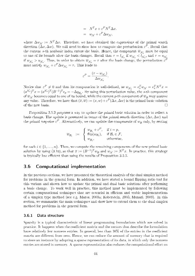
= NTx+ εPNT∆x.

= wN + εP∆wN ,

where ∆wN := NT∆x. Therefore, we have obtained the expressions of the primal searchdirection (∆x,∆w). We still need to show how to compute the perturbation εP . Recall thatthe current s-th nonbasic index enters the basis. Hence, the component wNs

must be equalto one of its bounds after the basis changes. Recall that τ = lNs

if wNs< lNs

, and τ = uNs

if wNs> uNs

. Thus, in order to obtain wNs= τ after the basis change, the perturbation εP

must satisfy wNs+ εP∆wNs

= τ . This leads to

εP =(τ − wNs

)

∆wNs

.

Notice that εP 6= 0 and that its computation is well-de�ned, as wNs= eTs wN = eTs N

Tx =

(aNs)Tx = (aNs)T (B−1)T ep = −∆yBp . By using this perturbation value, the s-th componentof wN becomes equal to one of its bound, while the current p-th component of wB may assumeany value. Therefore, we have that (x,w) := (x,w) +εP (∆x,∆w) is the primal basic solutionof the new basis.

Proposition 3.5.2 proposes a way to update the primal basic solution in order to re�ect abasis change. The update is presented in terms of the primal search direction (∆x,∆w) andthe primal step-size εP . Alternatively, we can update the components of wB only, by setting

wBi :=

wBi + εP , if i = p,

�ip(wBi), if Bi ∈ F ,wBi , otherwise,

for each i ∈ {1, . . . , n}. Then, we compute the remaining components of the new primal basicsolution by using (3.10), so that x := (B−1)TwB and wN := NTx. In practice, this strategyis typically less e�cient than using the results of Proposition 3.5.2.

3.6 Computational implementation

In the previous sections, we have presented the theoretical analysis of the dual simplex methodfor problems in the general form. In addition, we have stated a bound �ipping ratio test forthis variant and shown how to update the primal and dual basic solutions after performinga basis change. To work well in practice, this method must be implemented by followingcertain computational techniques that are essential in e�cient and stable implementationsof a simplex type method (see e.g. Maros, 2003a; Koberstein, 2005; Munari, 2009). In thissection, we summarize the main techniques and show how to extend them to the dual simplexmethod for problems in the general form.

3.6.1 Data structure

Sparsity is a typical characteristic of linear programming formulations which are solved inpractice. It happens when the coe�cient matrix and the vectors that describe the formulationhave relatively few nonzero entries. In general, less than 10% of the entries in the coe�cientmatrix are di�erent from zero. Hence, we can reduce the amount of memory that is requiredto store an instance by adopting a sparse representation of its data, in which only the nonzeroentries are stored in memory. A sparse representation also reduces the computational e�ort on

44

computations, as we avoid operations with zero values. In addition, we can exploit the sparsityof the auxiliary arrays used in the dual simplex method to compute, e.g., the basic solutionsand dual search direction. For a review on the main sparse representations used in simplextype methods, see Maros (2003a). In the implementation addressed here, we represent thecoe�cient matrix of the formulation by both the columnwise and the rowwise representations.Although it may sound redundant, this is a common strategy reported in the literature (Bixby,2002; Koberstein, 2008), as it allows to e�ciently access a matrix either by rows or by columns.These di�erent representations are important, because the performance of some operationsare superior when they access the matrix A rows, while others take advantage of columnwiseaccess.

Other operations in the dual simplex method also require carefully designed data struc-tures. For instance, consider the bound �ipping ratio test described in Section 3.5. Thebreakpoints of the dual objective function must be sorted before applying the ratio test. Inour implementation, we compute all these values and add them to a priority queue (heap),which keeps them partially sorted (see e.g. Aho et al., 1983). The breakpoints are then iter-atively removed from the queue until the conditions of Theorem 3.5.1 are satis�ed. We alsoneed special data structures to e�ciently solve linear systems of equations. This operationrequires an appropriate representation of the basic matrix as well as clever techniques forusing this representation to solve linear systems. We address this issue in the next subsection.

3.6.2 Representation of the basic matrix

Currently, e�cient implementations of simplex-type methods represent the basic matrix byusing the LU factorization and the LU update strategies as proposed by Suhl and Suhl (1990)and Suhl and Suhl (1993). Although the LU factorization is widely used for representingmatrices and solving linear systems in many other subjects, the techniques presented by theseauthors are speci�c for simplex-type methods, specially the update of the representation afterperforming basis change. In this section, we extend the Suhl and Suhl techniques to thecontext of the dual simplex method for problems in the general form.

SSLU Factorization

The LU factorization proposed by Suhl and Suhl (1990), which we call SSLU factorization,consists in transforming the basic matrix B in a matrix U , by using t < n elementary matricesL1, L2, . . . , Lt, such that

LtLt−1 . . . L1B = L−1B = U ⇒ B = LU . (3.42)

By elementary matrices we mean those that di�er from the identity by a single column, andthis column has all the entries above the main diagonal equal to zero. For the factorization ofB, we may need additional row and column permutation matrices, which we denote respec-tively by P and Q. These matrices are helpful to express the factors L and U as triangularmatrices L and U such that

L = PLP−1 and U = PUQ. (3.43)

With this notation, we have PBQ = LU . By convention, L is a lower triangular matrix withunitary diagonal, while U is upper triangular. This nomenclature is extended to L and U ,which are called the permuted triangular factors. L is a permuted lower triangular matrix,and U is a permuted upper triangular matrix.

The position of the columns in the basic matrix is given by the order of the indices in theset B. Hence, the permutation that is determined by matrix Q can be applied directly to B,

45

instead of being used in the LU factorization. Indeed, if we post-multiply both sides of theequality L−1B = U by the product QP , we obtain

L−1B(QP ) = U(QP ) = P−1UQ−1(QP ) = P−1UP.

Then, we reorder the columns of B and U using the permutation QP , such that B := BQPand U := UQP . As a result, we obtain L−1B = U as before, but now U = PUP−1 andtherefore matrix Q can be discarded. We say that the triangular factor U is obtained fromU by means of symmetric permutations, as P−1 = P T . All the pivot elements lay on thismain diagonal, which is a useful feature for solving linear systems and for updating therepresentation after a basis change.

SSLU update

After each basis change, a column of the basic matrix must be replaced by the column ofthe variable that enters the basis. This change requires a new factorization of the basismatrix, which can be computed from scratch. However, to factorize the basic matrix fromscratch is a computationally expensive operation in general. By observing this, Suhl and Suhl(1993) proposed a clever strategy for e�ciently update it. This strategy has a relatively smallcomputational cost and in addition seeks to maintain the sparsity and the numerical stabilityof the factorization.

Consider that the basic matrix B is represented by the factors L−1 and U , which havebeen obtained by the SSLU factorization. Suppose that, after a basis change, column aNs

has been chosen to enter the basis at position p, so the new basic matrix is given by B =[b1, . . . , bp−1, a

Ns , bp+1, . . . , bn]. If we premultiply this matrix by L−1, then we obtain

L−1B =[L−1b1, . . . , L

−1bp−1, L−1aq, L−1bp+1, . . . , L

−1bn

]=

[u1, . . . , up−1, g, up+1, . . . , un

].

Therefore, if we replace the p-th column of U by the column g = L−1aNs , then the previouspermuted triangle factors can be used to represent the new basic matrix. However, sincethe column g may have nonzero values at any position, we cannot guarantee that the corre-sponding matrix U remains triangular with this new column. To overcome this, the SSLUupdate procedure uses an elementary matrix to eliminate the entries of g which are belowthe pivot entry. Then, by using symmetric permutations of the rows and columns of U , thecorresponding matrix U recovers the triangular form. The elementary matrix that is usedto eliminate entries must be included in the representation of L−1. In practice, the imple-mentation should impose a maximum number of elementary matrices that can be used in therepresentation. When this maximum is achieved, the factorization of the basic matrix mustbe recomputed from scratch. The refactorization may be motivated by other reasons as well,such as when a maximum number of updates is achieved, or when the numerical instabilityof the factorization is detected.

Solving linear systems

In the SSLU factorization, we use the factors L−1 = LtLt−1 . . . L1 and U to compute thesolution of linear systems involving the basic matrix. The factor L−1 is represented as aproduct of t elementary matrices. The solution α of a linear system of type Bα = υ isobtained by an operation that is called forward transformation (FTRAN). This operationconsists in the following two steps:

46

(i) Compute υ0 = Lt . . . L1υ;

(ii) Solve Uα = υ0.

In (ii), the corresponding triangular representation of the factor U should be used. Speci�cally,the permutation should be applied to the components of υ and α prior to the computations.Hence, the solution is given by

αi =1

uii

υi − n∑j=i+1

uijαj

, i = n, n− 1, . . . , 1.

where υ and α denotes the respective permuted vectors. Observe in this expression that eachcomponent αj multiplies only the column j of U . Therefore, if αj = 0, then the computationmay skip column uj .

We are also interested in solving linear systems of the type BTα = υ. In this case, thesolution α is obtained by the backward transformation (BTRAN)

(i) Solve UTα0 = υ;

(ii) Compute α = LT1 . . . LTt α

0.

Step (i) consists in solving a linear system with an upper triangular matrix, which means thatthe permutation P should be applied to UT . Then, we actually solve the system UT α0 = υ,which has the solution

α0j =

1

ujj

(υj −

j−1∑i=1

uijα0i

), j = 1, 2, . . . , n.

Similarly to what is done in the FTRAN, if α0i = 0 then the i-th row of U is skipped in the

computations. Finally, the elementary matrices are applied in order to obtain the solution α.

Data structure

Fig. 3.4 illustrates the data structure that we use to store the factors L−1 = LtLt−1 . . . L1

and U in our implementation. It follows the discussions presented in Suhl and Suhl (1990,1993); Koberstein (2005). The permuted triangular factor U is stored using both columnwiseand rowwise forms. For each entry in U , there is a pointer linking its position in the rowwiserepresentation to its position in the columnwise representation. By using these pointers, weavoid searching for a given entry of the matrix, a operation that would slow down the fac-torization and updating procedures. The gray areas in the �gure represent free regions whichare used to store nonzero entries that are created during the SSLU update. The elementarymatrices LtLt−1 . . . L1 are stored in the last positions of the rowwise representation. Only theentries in nontrivial columns/rows of these matrices are stored.

3.6.3 Scaling

Scaling is an essential operation to avoid numerical instability in a simplex-type method. Itconsists in modifying the coe�cient matrix of the problem in order to obtain a matrix withbetter numerical characteristics. The modi�cation involves multiplying rows and columnsby scaling factors, without modifying the set of optimal solutions of the problem. Manyscaling techniques are proposed in the literature, and they di�er basically in how to compute

47

t ... 1

z ... NNZ

4 ... 7

: position

1 ... 5 6 7 ... ... k k+1 ... ... ... z-1 z NNZ

j11 j21 j22 j23 ... ji1 ji2 ... lt2 lt1 ... l11

ũ1 ũ

2 ... ũi ... Lt ... L1

* * * * * * * *

: ind_pivot

S L’

U’

S

U’

r

r

l

r

r

l

l l r

r

l

l r

r

l

l

S

U’

U

t

1 2 ... i ... n

1 5 ... k ... ...

1 3 ... 2 ... ...

pos_row:

ind_col:

n_row:

value_row:

Rowwise

representation

pointer_col:

* * * * * * * *

ũ1 ũ2 ... ũj ...

i11 i12 i21 i22 i23 ... ij1 ij2 ... 1 2 .. ... 4 5 6 ... ... r r+1 ... ... ...

2 3 ... 2

1 4 ... r 1 2 ... j ... n

pos_col:

ind_lin:

n_col:

value_col:

Columnwise representation

pointer_row:

Figure 3.4: Data structure that stores the permuted triangular factors.

the scaling factors. Munari and Arenales (2009) present a review of the scaling techniquesthat are most used in implementations of simplex-type methods. In addition, the authorscompare the performance of the techniques when solving the Netlib instances by simplex-typemethods. According to the reported results, the geometric average scaling and the scalingtechnique proposed by Benichou et al. (1977) are the best strategies concerning CPU timeand numerical stability. In the implementation of the dual simplex method for problems inthe general form, we have tested all the scaling techniques reviewed by Munari and Arenales(2009). Among them, the geometric average scaling led to the best overall performance of themethod. Hence, this technique has been adopted as default in our implementation.

3.6.4 Numerical tolerances

Approximations are inevitable when making computations with fractional values in a com-puter. Due to the �oating point representations, the approximations may happen in theassignment of values to variables as well as during calculations. Based on this, we shouldbe careful when comparing two given values, and use a tolerance in the comparisons. Forinstance, to verify if the values a and b are equal, we should actually verify if |a − b| < δ,where δ is a tolerance which guarantees that the values are su�ciently close to each other. Ingeneral, the appropriate choice of δ depends on the type of comparison and the magnitude ofthe values. The di�erent tolerance values used in our implementation are described in Table3.1, according to their usage.

3.7 Results and discussion

In this section, we analyze the practical performance of the dual simplex method for problemsin the general form (DSMGF). The experiments are based on benchmarking instances from theNetlib, a public repository of linear programming problems. First, we compare two variantsof the DSMGF in order to verify the impact of the bound �ipping ratio test in relation tothe standard ratio test. Then, the variant with the best overall performance is compared

48

Tolerance Usage

10−6 minimum absolute value allowed for the pivot10−1 minimum relative value allows for the pivot10−6 primal feasibility test (pricing operation)10−9 dual feasibility test (ratio test)10−10 zero tolerance10−14 drop tolerance (reset the value as zero)

Table 3.1: Numerical tolerances used in our computational implementation.

against other standard simplex-type methods. We have implemented all the methods in theC programming language, including the procedures to factorize and update the basic matrix.The experiments were performed on a Linux PC with an Intel Core i7 2.8 GHz CPU and 8.0GB of memory.

The Netlib is a repository of linear programming problems, which is widely used to bench-mark simplex-type methods. Many instances in this set correspond to real-life problems thatare very challenging to simplex-type methods. To solve these problems e�ciently, it is im-portant to exploit the sparsity of the data and to use techniques for controlling the numericalstability of the method. The instances are publicly available at http://www.netlib.org/lp/data. Tables 3.2 and 3.3 summarize the main information regarding the instances. Columnsn andm give the number of variables and the number of nontrivial constraints in the instance,respectively. The remaining columns are the number of variables that are free (f), that haveonly one �nite bound (p), and that are boxed (b), considering the problem is formulated inthe general form. Similar columns are presented to describe the types of constraints. Thenumber of �xed variables are shown inside parenthesis in column (b). This value is omitted incase it is zero. The density of the coe�cient matrix (d) and the optimal value of the instanceare given in the last two columns. For further information regarding these instances, pleasesee Koch (2004); Gay (1997).

3.7.1 Checking the impact of the bound �ipping ratio test

In the �rst set of computational experiments, we verify the importance of using the bound�ipping ratio test in the DSMGF. We have solved the Netlib instances by using two variantsof the DSMGF: one using the standard ratio test and another using the bound �ipping ratiotest. We refer to these variants as DSMGF-SRT and DSMGF-BFRT, respectively. Tables3.4 and 3.5 show the number of iterations and the CPU time (in seconds) to solve the Netlibinstances by using the two variants of the DSMGF. The total number of iterations and thetotal CPU time to solve all the instances are presented in the last row of Table 3.5. Accordingto the results, the bound �ipping ratio test was helpful to reduce the number of iterationsto solve the instances. Moreover, the variant using the bound �ipping ratio test was able tosolve all instances, while the other variant failed in 3 instances (due to numerical di�culties).In the vast majority of instances, the variant with the standard ratio test (DSMGF-SRT)presented a larger number of iterations and, in total, it required 44% more iterations inrelation to the DSMGF-BFRT. The largest impact of the bound �ipping ratio test is observedfor the instances FIT2D, FIT1D, PDS-06, KEN-18. These are instances in which most of thevariables and constraints are boxed, which bene�ts the bound �ipping (see Theorem 3.5.1).The bound �ipping ratio test also contributed to reduce the CPU time in many instances. Intotal, the DSMGF-BFRT was 2.15 times faster than the other variant. Therefore, the results

49

Variables Constraints

Problem n m f p b p b d (%) Optimal value

25FV47 1571 821 0 1571 0 305 516 0.806 5.5018458883E+03

80BAU3B 9799 2262 0 6315 3484 (498) 2262 0 0.095 9.8722419241E+05

ADLITTLE 97 56 0 97 0 41 15 7.051 2.2549496316E+05

AFIRO 32 27 0 32 0 19 8 9.606 -4.6475314286E+02

AGG 163 488 0 163 0 452 36 3.030 -3.5991767287E+07

AGG2 302 516 0 302 0 456 60 2.749 -2.0239252356E+07

AGG3 302 516 0 302 0 456 60 2.759 1.0312115935E+07

BANDM 472 305 0 472 0 0 305 1.732 -1.5862801845E+02

BEACONFD 262 173 0 262 0 33 140 7.446 3.3592485807E+04

BLEND 83 74 0 83 0 31 43 7.994 -3.0812149846E+01

BNL1 1175 643 0 1175 0 411 232 0.678 1.9776295615E+03

BNL2 3489 2324 0 3489 0 997 1327 0.173 1.8112365404E+03

BOEING1 384 351 0 228 156 253 98 2.593 -3.3521356751E+02

BOEING2 143 166 0 89 54 143 23 5.038 -3.1501872802E+02

BORE3D 315 233 0 303 12 (1) 19 214 1.947 1.3730803942E+03

BRANDY 249 220 0 249 0 54 166 3.921 1.5185098965E+03

CAPRI 353 271 14 192 147 (16) 129 142 1.847 2.6900129138E+03

CRE-A 4067 3516 0 4067 0 3181 335 0.105 2.3595407061E+07

CRE-B 72447 9648 0 72447 0 4690 4958 0.037 2.3129639887E+07

CRE-C 3678 3068 0 3678 0 2733 335 0.117 2.5275116141E+07

CRE-D 69980 8926 0 69980 0 3968 4958 0.039 2.4454969765E+07

CYCLE 2857 1903 7 2773 77 514 1389 0.381 -5.2263930249E+00

CZPROB 3523 929 0 3294 229 (229) 39 890 0.326 2.1851966989E+06

D2Q06C 5167 2171 0 5167 0 664 1507 0.289 1.2278421081E+05

D6CUBE 6184 415 0 6184 0 0 415 1.469 3.1549166667E+02

DEGEN2 534 444 0 534 0 223 221 1.678 -1.4351780000E+03

DEGEN3 1818 1503 0 1818 0 786 717 0.902 -9.8729400000E+02

E226 282 223 0 282 0 190 33 4.099 -1.8751929066E+01

ETAMACRO 688 400 0 471 217 (82) 128 272 0.875 -7.5571523337E+02

FFFFF800 854 524 0 854 0 174 350 1.392 5.5567956482E+05

FINNIS 614 497 0 533 81 (45) 450 47 0.757 1.7279106560E+05

FIT1D 1026 24 0 0 1026 23 1 54.435 -9.1463780924E+03

FIT1P 1677 627 0 1278 399 0 627 0.938 9.1463780924E+03

FIT2D 10500 25 0 0 10500 24 1 49.150 -6.8464293294E+04

FIT2P 13525 3000 0 6025 7500 0 3000 0.124 6.8464293294E+04

FORPLAN 421 161 0 397 24 (3) 70 91 6.732 -6.6421896127E+02

GANGES 1681 1309 0 1284 397 25 1284 0.314 -1.0958573613E+05

GFRD-PNC 1092 616 0 834 258 68 548 0.353 6.9022359995E+06

GREENBEA 5405 2392 0 5012 393 (103) 193 2199 0.239 -7.2555248130E+07

GREENBEB 5405 2392 4 4995 406 (115) 193 2199 0.239 -4.3022602612E+06

GROW15 645 300 0 45 600 0 300 2.904 -1.0687094129E+08

GROW22 946 440 0 66 880 0 440 1.983 -1.6083433648E+08

GROW7 301 140 0 21 280 0 140 6.198 -4.7787811815E+07

ISRAEL 142 174 0 142 0 174 0 9.183 -8.9664482186E+05

KB2 41 43 0 32 9 27 16 16.222 -1.7499001299E+03

KEN-07 3602 2426 0 0 3602 0 2426 0.096 -6.7952044338E+08

KEN-11 21349 14694 0 0 21349 0 14694 0.016 -6.9723822625E+09

KEN-13 42659 28632 0 0 42659 0 28632 0.008 -1.0257394789E+10

KEN-18 154699 105127 0 0 154699 0 105127 0.002 -5.2217025287E+10

LOTFI 308 153 0 308 0 58 95 2.288 -2.5264706062E+01

MAROS 1443 846 0 1408 35 523 323 0.788 -5.8063743701E+04

MAROS-R7 9408 3136 0 9408 0 0 3136 0.491 1.4971851665E+06

MODSZK1 1620 687 2 1618 0 0 687 0.285 3.2061972906E+02

NESM 2923 662 0 1240 1683 (175) 94 568 0.687 1.4076036488E+07

OSA-07 23949 1118 0 23949 0 1118 0 0.537 5.3572251730E+05

OSA-14 52460 2337 0 52460 0 2337 0 0.257 1.1064628447E+06

Table 3.2: Description of the Netlib instances. (Part 1)

50

Variables Constraints

Problem n m f p b p b d (%) Optimal value

OSA-30 100024 4350 0 100024 0 4350 0 0.138 2.1421398732E+06

OSA-60 232966 10280 0 232966 0 10280 0 0.058 4.0440725032E+06

PDS-02 7535 2953 0 5401 2134 181 2772 0.074 2.8857862010E+10

PDS-06 28655 9881 0 19415 9240 696 9185 0.022 2.7761037600E+10

PDS-10 48763 16558 0 32615 16148 1169 15389 0.013 2.6727094976E+10

PDS-20 105728 33874 0 70840 34888 2447 31427 0.006 2.3821658640E+10

PEROLD 1376 625 88 958 330 (64) 130 495 0.700 -9.3807552782E+03

PILOT 3652 1441 0 2409 1243 (167) 1208 233 0.820 -5.5748972928E+02

PILOT.JA 1988 940 88 1250 650 (311) 279 661 0.787 -6.1131364656E+03

PILOT.WE 2789 722 80 2337 372 (78) 139 583 0.453 -2.7201075328E+06

PILOT4 1000 410 88 635 277 (30) 123 287 1.254 -2.5811392589E+03

PILOT87 4883 2030 0 3085 1798 (180) 1797 233 0.738 3.0171034733E+02

PILOTNOV 2172 975 0 1628 544 (204) 274 701 0.617 -4.4972761882E+03

RECIPE 180 91 0 85 95 (24) 24 67 4.048 -2.6661600000E+02

SC105 103 105 0 103 0 60 45 2.589 -5.2202061212E+01

SC205 203 205 0 203 0 114 91 1.324 -5.2202061212E+01

SC50A 48 50 0 48 0 30 20 5.417 -6.4575077059E+01

SC50B 48 50 0 48 0 30 20 4.917 -7.0000000000E+01

SCAGR25 500 471 0 500 0 171 300 0.660 -1.4753433061E+07

SCAGR7 140 129 0 140 0 45 84 2.326 -2.3313898243E+06

SCFXM1 457 330 0 457 0 143 187 1.717 1.8416759028E+04

SCFXM2 914 660 0 914 0 286 374 0.859 3.6660261565E+04

SCFXM3 1371 990 0 1371 0 429 561 0.573 5.4901254550E+04

SCORPION 358 388 0 358 0 108 280 1.027 1.8781248227E+03

SCRS8 1169 490 0 1169 0 106 384 0.556 9.0429695380E+02

SCSD1 760 77 0 760 0 0 77 4.081 8.6666666743E+00

SCSD6 1350 147 0 1350 0 0 147 2.175 5.0500000077E+01

SCSD8 2750 397 0 2750 0 0 397 0.786 9.0499999993E+02

SCTAP1 480 300 0 480 0 180 120 1.175 1.4122500000E+03

SCTAP2 1880 1090 0 1880 0 620 470 0.328 1.7248071429E+03

SCTAP3 2480 1480 0 2480 0 860 620 0.242 1.4240000000E+03

SEBA 1028 515 0 521 507 1 514 0.822 1.5711600000E+04

SHARE1B 225 117 0 225 0 28 89 4.372 -7.6589318579E+04

SHARE2B 79 96 0 79 0 83 13 9.151 -4.1573224074E+02

SHELL 1775 536 0 1408 367 (250) 2 534 0.374 1.2088253460E+09

SHIP04L 2118 402 0 2118 0 48 354 0.744 1.7933245380E+06

SHIP04S 1458 402 0 1458 0 48 354 0.743 1.7987147004E+06

SHIP08L 4283 778 0 4283 0 80 698 0.384 1.9090552114E+06

SHIP08S 2387 778 0 2387 0 80 698 0.383 1.9200982105E+06

SHIP12L 5427 1151 0 5427 0 106 1045 0.259 1.4701879193E+06

SHIP12S 2763 1151 0 2763 0 106 1045 0.257 1.4892361344E+06

SIERRA 2036 1227 0 0 2036 699 528 0.292 1.5394362184E+07

STAIR 467 356 6 373 88 (82) 147 209 2.319 -2.5126695119E+02

STANDATA 1075 359 0 955 120 (16) 199 160 0.785 1.2576995000E+03

STANDMPS 1075 467 0 955 120 (16) 199 268 0.733 1.4060175000E+03

STOCFOR1 111 117 0 111 0 54 63 3.442 -4.1131976219E+04

STOCFOR2 2031 2157 0 2031 0 1014 1143 0.190 -3.9024408538E+04

STOCFOR3 15695 16675 0 15695 0 7846 8829 0.030 -3.9976783944E+04

TRUSS 8806 1000 0 8806 0 0 1000 0.316 4.5881584719E+05

TUFF 587 333 2 556 29 (3) 41 292 2.312 2.9214776509E-01

VTP.BASE 203 198 1 119 83 (18) 143 55 2.259 1.2983146246E+05

WOOD1P 2594 244 0 2594 0 1 243 11.094 1.4429024116E+00

WOODW 8405 1098 0 8405 0 13 1085 0.406 1.3044763331E+00

Table 3.3: Description of the Netlib instances. (Part 2)

51

indicate that the DSMGF-BFRT outperforms the DSMGF-SRT. For this reason, we adoptthe bound �ipping ratio test as default in the experiments we report in the next sections.

3.7.2 Comparing against standard simplex-type methods

The second set of experiments consisted in comparing the performance of the DSMGF (withbound �ipping ratio test) against the performance of standard simplex-type methods, namelythe primal simplex method for problems in the standard form (PSMSF) and the dual simplexmethod for problems in the standard form (DSMSF). By standard form we refer to a formu-lation in which the constraints are modeled by a set of equations (see Chapter 2). Beforesolving a problem in the standard, we usually need to the transform inequalities and boxedconstraints into equalities, by means of slack or surplus variables.

We have implemented both the PSMSF and the DSMSF, following the descriptions inMunari (2009) and Maros (2003a). The implementation has the same (or very similar) datastructures and computational techniques as those used in the implementation of the DSMGF.Hence, all the methods rely on the same implementation of core components and we havespecialized the code according to each variant. This allows us to verify the performance of thedi�erent variants without having the results biased to the level of the implementation skills.It is worth mentioning that in our implementation of the DSMSF, we also use the bound�ipping ratio test as default.

Tables 3.4 and 3.5 show the number of iterations and the CPU time in seconds to solvethe Netlib instances by the three variants. First, we observe that the PSMSF is clearlyoutperformed by the other two variants. A strong reason for that is the use of the bound�ipping ratio test in the dual variants, as no equivalent strategy is available for the primalmethod. Indeed, dual simplex-type methods have been recognized as superior in the literature(Bixby, 2002; Maros, 2003b; Koberstein, 2008). A very similar performance is observed forthe two dual variants, the DSMSF and the DSMGF, with the latter presenting slightly betterresults. The DSMGF was the fastest variant in many di�cult instances, such as CRE-B,PDS-10 and KEN-18. In total, the DSMGF was 10% faster than the DSMSF.


In this chapter, we addressed a variant of the dual simplex method which exploits specialproperties of the general form. First, we presented a novel theoretical discussion of the variant,which extends the preliminary studies of Arenales (1984), Sousa et al. (2005) and Silva et al.(2007). Then, we discussed the main techniques that are useful to obtain an e�cient andstable implementation of the method. Finally, we presented computational experiments withthe Netlib instances, which are widely used to benchmark simplex-type methods. The resultsindicate that the dual simplex method for problems in the general form is competitive withthe standard dual simplex method and outperforms the standard primal simplex method.In particular, the proposed method has the best relative performance in many of the mostdi�cult instances, namely CRE-B, PDS-10 and KEN-18.

Further topics can be investigated regarding the dual simplex method for problems in thegeneral form. First, the performance of the method should be veri�ed for larger instances,specially those corresponding to relaxations of integer programming problems. Also, it wouldbe interesting to see the behavior of the method within integer programming methodologies,such as the branch-and-bound method and the cutting plane method. Furthermore, it isimportant to investigate strategies for obtaining advanced basis to initialize the method.

52

DSMGF-SRT DSMGF-BFRT

Instance Iterations Time (in s) Iterations Time (in s)

25FV47 4568 0.62 4656 0.64

80BAU3B 7992 2.01 4464 0.79

ADLITTLE 136 0.01 150 0.00

AFIRO 32 0.00 37 0.00

AGG 323 0.03 322 0.05

AGG2 375 0.02 385 0.03

AGG3 382 0.04 392 0.03

BANDM 700 0.07 648 0.07

BEACONFD 111 0.01 111 0.02

BLEND 118 0.01 136 0.00

BNL1 1661 0.20 1796 0.24

BNL2 3057 0.43 3105 0.44

BOEING1 1018 0.11 662 0.08

BOEING2 261 0.03 254 0.01

BORE3D 249 0.02 260 0.03

BRANDY 453 0.04 474 0.06

CAPRI 416 0.03 307 0.03

CRE-A 2900 0.44 3040 0.44

CRE-B 40243 85.09 43655 86.88

CRE-C 2910 0.46 2800 0.40

CRE-D 39164 77.39 38537 69.03

CYCLE 3841 0.55 3201 0.46

CZPROB 3156 0.44 3121 0.44

D2Q06C 22764 6.03 21994 4.61

D6CUBE 1118 0.26 1186 0.27

DEGEN2 2497 0.27 2386 0.25

DEGEN3 12554 1.87 12247 1.76

E226 490 0.05 440 0.05

ETAMACRO 1082 0.12 832 0.10

FFFFF800 852 0.08 1083 0.12

FINNIS 461 0.05 436 0.05

FIT1D 612 0.07 85 0.01

FIT1P 3931 0.53 3685 0.51

FIT2D 6951 3.03 207 0.11

FIT2P 48748 54.14 31659 29.95

FORPLAN 276 0.01 273 0.02

GANGES 1468 0.20 1326 0.17

GFRD-PNC 644 0.08 541 0.07

GREENBEA 14290 3.75 13237 2.92

GREENBEB 14708 3.51 15779 3.30

GROW15 763 0.07 3033 0.39

GROW22 1748 0.23 4691 0.65

GROW7 394 0.04 726 0.09

ISRAEL 197 0.02 175 0.00

KB2 53 0.00 43 0.02

KEN-07 5237 0.78 3189 0.39

KEN-11 34608 32.65 20379 15.08

KEN-13 108475 242.98 57089 111.07

KEN-18 472306 4619.39 193303 1847.87

LOTFI 389 0.03 536 0.04

MAROS 2669 0.36 2839 0.39

MAROS-R7 4934 5.64 4980 5.33

MODSZK1 � � 679 0.08

NESM 3413 0.47 1910 0.25

OSA-07 1048 0.76 1048 1.34

OSA-14 2511 4.26 2503 4.48

Table 3.4: Number of iterations and CPU time (in seconds) to solve the Netlib instances by usingtwo variants of the dual simplex method for problems in the general form: one usingthe standard ration test (DSMGF-SRT) and another using the bound �ipping ratio test(DSMGF-BFRT). (Part 1)

53

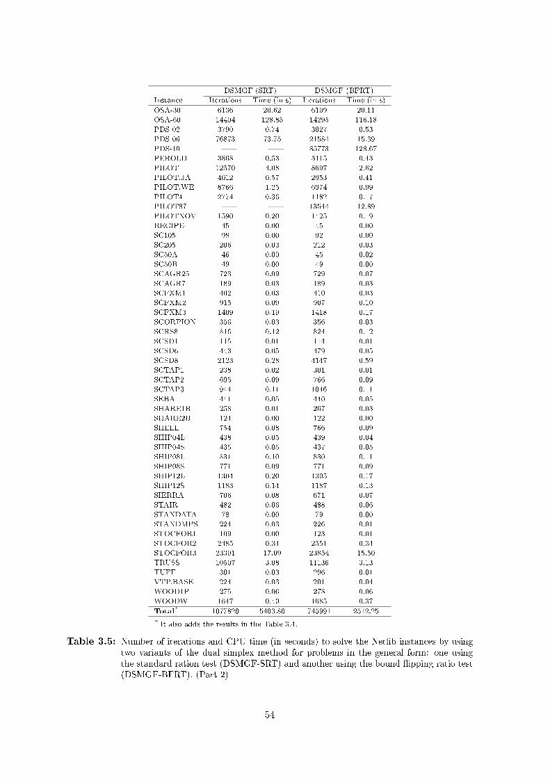
DSMGF (SRT) DSMGF (BFRT)

Instance Iterations Time (in s) Iterations Time (in s)

OSA-30 6136 20.62 6109 20.11

OSA-60 14404 128.85 14295 116.18

PDS-02 3790 0.74 3027 0.53

PDS-06 76873 73.75 21584 15.39

PDS-10 � � 85773 128.67

PEROLD 3868 0.53 3115 0.43

PILOT 12570 4.08 8697 2.62

PILOT.JA 4012 0.57 2953 0.41

PILOT.WE 8766 1.25 6974 0.99

PILOT4 2774 0.36 1182 0.17

PILOT87 � � 13544 12.89

PILOTNOV 1590 0.20 1425 0.19

RECIPE 45 0.00 45 0.00

SC105 98 0.00 92 0.00

SC205 206 0.03 212 0.03

SC50A 46 0.00 45 0.02

SC50B 49 0.00 49 0.00

SCAGR25 723 0.09 729 0.07

SCAGR7 189 0.03 189 0.03

SCFXM1 402 0.03 410 0.03

SCFXM2 915 0.09 907 0.10

SCFXM3 1409 0.19 1418 0.17

SCORPION 356 0.03 356 0.03

SCRS8 816 0.12 824 0.12

SCSD1 115 0.01 114 0.01

SCSD6 443 0.05 479 0.05

SCSD8 2123 0.28 4147 0.59

SCTAP1 238 0.02 301 0.01

SCTAP2 695 0.09 766 0.09

SCTAP3 944 0.11 1046 0.11

SEBA 441 0.05 440 0.05

SHARE1B 258 0.01 267 0.03

SHARE2B 124 0.00 122 0.00

SHELL 754 0.08 766 0.09

SHIP04L 438 0.05 439 0.04

SHIP04S 435 0.05 437 0.05

SHIP08L 831 0.10 830 0.11

SHIP08S 771 0.09 771 0.09

SHIP12L 1304 0.20 1305 0.17

SHIP12S 1183 0.14 1187 0.13

SIERRA 706 0.08 671 0.07

STAIR 482 0.06 488 0.06

STANDATA 78 0.00 79 0.00

STANDMPS 224 0.03 226 0.01

STOCFOR1 109 0.00 123 0.01

STOCFOR2 2485 0.34 2551 0.34

STOCFOR3 23391 17.09 23854 15.50

TRUSS 10507 3.08 11136 3.13

TUFF 301 0.03 296 0.01

VTP.BASE 224 0.03 201 0.04

WOOD1P 275 0.06 278 0.06

WOODW 1647 0.40 1685 0.37

Total* 1077820 5403.80 745991 2512.25

* It also adds the results in the Table 3.4.

Table 3.5: Number of iterations and CPU time (in seconds) to solve the Netlib instances by usingtwo variants of the dual simplex method for problems in the general form: one usingthe standard ration test (DSMGF-SRT) and another using the bound �ipping ratio test(DSMGF-BFRT). (Part 2)

54

PSMSF DSMSF DSMGF

Instance Iterations Time (in s) Iterations Time (in s) Iterations Time (in s)

25FV47 6605 0.92 4962 0.69 4656 0.64

80BAU3B 9447 1.87 4306 0.86 4464 0.79

ADLITTLE 134 0.00 141 0.01 150 0.00

AFIRO 23 0.00 37 0.00 37 0.00

AGG 122 0.02 194 0.02 322 0.05

AGG2 193 0.03 277 0.02 385 0.03

AGG3 174 0.01 279 0.03 392 0.03

BANDM 591 0.06 605 0.06 648 0.07

BEACONFD 112 0.00 111 0.00 111 0.02

BLEND 95 0.01 133 0.01 136 0.00

BNL1 2239 0.28 1872 0.22 1796 0.24

BNL2 6720 1.58 2998 0.43 3105 0.44

BOEING1 680 0.10 579 0.06 662 0.08

BOEING2 174 0.02 249 0.02 254 0.01

BORE3D 211 0.03 204 0.01 260 0.03

BRANDY 361 0.06 515 0.06 474 0.06

CAPRI 509 0.08 308 0.03 307 0.03

CRE-A 4164 1.14 2830 0.40 3040 0.44

CRE-B 261002 776.97 40420 115.33 43655 86.88

CRE-C 4844 0.77 2913 0.41 2800 0.40

CRE-D 63757 160.39 30928 73.14 38537 69.03

CYCLE 1121 0.33 2935 0.42 3201 0.46

CZPROB 1965 0.26 1688 0.24 3121 0.44

D2Q06C 33194 10.86 22293 6.15 21994 4.61

D6CUBE 204300 61.25 1022 0.27 1186 0.27

DEGEN2 4665 0.52 1943 0.21 2386 0.25

DEGEN3 194262 33.73 10175 1.50 12247 1.76

E226 561 0.06 475 0.05 440 0.05

ETAMACRO 720 0.06 870 0.08 832 0.10

FFFFF800 990 0.12 981 0.11 1083 0.12

FINNIS 690 0.08 426 0.04 436 0.05

FIT1D 1058 0.12 85 0.01 85 0.01

FIT1P 4165 0.57 3685 0.48 3685 0.51

FIT2D 11500 6.99 260 0.15 207 0.11

FIT2P 92356 56.02 31919 12.93 31659 29.95

FORPLAN 264 0.01 274 0.01 273 0.02

GANGES 1613 0.17 1305 0.16 1326 0.17

GFRD-PNC 1065 0.11 541 0.06 541 0.07

GREENBEA 17265 4.18 10091 2.41 13237 2.92

GREENBEB 13341 3.18 17706 4.11 15779 3.30

GROW15 791 0.10 2614 0.32 3033 0.39

GROW22 1256 0.17 5670 0.77 4691 0.65

GROW7 330 0.02 714 0.09 726 0.09

ISRAEL 161 0.03 168 0.01 175 0.00

KB2 71 0.00 43 0.00 43 0.02

KEN-07 4320 0.62 3177 0.47 3189 0.39

KEN-11 30461 31.12 20352 19.72 20379 15.08

KEN-13 88288 216.14 55838 133.23 57089 111.07

KEN-18 361040 4495.67 199352 2058.71 193303 1847.87

LOTFI 286 0.02 493 0.06 536 0.04

MAROS 1664 0.20 2571 0.34 2839 0.39

MAROS-R7 3897 2.74 4995 6.03 4980 5.33

MODSZK1 1085 0.12 688 0.06 679 0.08

NESM 4465 0.58 2127 0.27 1910 0.25

OSA-07 804 0.39 1047 1.17 1048 1.34

OSA-14 1666 1.89 2505 3.45 2503 4.48

Table 3.6: Number of iterations and CPU time (in seconds) to solve the Netlib instances by usingthree simplex type methods: the primal simplex method for problems in the standardform (PSMSF), the dual simplex method for problems in the standard form (DSMSF),and the dual simplex method for problems in the general form (DSMGF). (Part 1)

55

PSMSF DSMSF DSMGF

Instance Iterations Time (in s) Iterations Time (in s) Iterations Time (in s)

OSA-30 3274 7.33 6087 16.28 6109 20.11

OSA-60 7278 38.49 14878 94.39 14295 116.18

PDS-02 8196 1.65 3067 0.49 3027 0.53

PDS-06 83266 78.06 23911 15.83 21584 15.39

PDS-10 172734 334.97 107472 160.31 85773 128.67

PEROLD 6267 0.86 2957 0.39 3115 0.43

PILOT 11856 5.71 8367 2.81 8697 2.62

PILOT.JA 7437 1.05 3209 0.45 2953 0.41

PILOT.WE 9063 1.27 6538 0.95 6974 0.99

PILOT4 1289 0.16 1250 0.14 1182 0.17

PILOT87 19791 17.64 12130 11.65 13544 12.89

PILOTNOV 2760 0.38 1402 0.18 1425 0.19

RECIPE 51 0.00 45 0.00 45 0.00

SC105 114 0.02 92 0.00 92 0.00

SC205 245 0.02 202 0.02 212 0.03

SC50A 50 0.01 45 0.00 45 0.02

SC50B 50 0.00 49 0.00 49 0.00

SCAGR25 585 0.05 688 0.06 729 0.07

SCAGR7 165 0.01 177 0.02 189 0.03

SCFXM1 393 0.05 406 0.03 410 0.03

SCFXM2 794 0.07 903 0.10 907 0.10

SCFXM3 1187 0.14 1402 0.17 1418 0.17

SCORPION 377 0.05 347 0.05 356 0.03

SCRS8 686 0.07 592 0.06 824 0.12

SCSD1 304 0.02 109 0.00 114 0.01

SCSD6 784 0.08 456 0.04 479 0.05

SCSD8 1940 0.25 2894 0.39 4147 0.59

SCTAP1 266 0.02 310 0.04 301 0.01

SCTAP2 902 0.11 745 0.07 766 0.09

SCTAP3 1232 0.17 1047 0.12 1046 0.11

SEBA 501 0.06 440 0.05 440 0.05

SHARE1B 283 0.02 265 0.03 267 0.03

SHARE2B 131 0.00 121 0.00 122 0.00

SHELL 814 0.08 759 0.07 766 0.09

SHIP04L 583 0.05 414 0.02 439 0.04

SHIP04S 510 0.05 418 0.03 437 0.05

SHIP08L 1078 0.14 810 0.10 830 0.11

SHIP08S 832 0.10 732 0.09 771 0.09

SHIP12L 1564 0.21 1288 0.17 1305 0.17

SHIP12S 1194 0.16 1185 0.15 1187 0.13

SIERRA 1062 0.13 670 0.07 671 0.07

STAIR 839 0.11 482 0.05 488 0.06

STANDATA 71 0.00 73 0.00 79 0.00

STANDMPS 380 0.04 211 0.01 226 0.01

STOCFOR1 117 0.00 118 0.02 123 0.01

STOCFOR2 2883 0.40 2402 0.32 2551 0.34

STOCFOR3 35221 33.24 21395 13.39 23854 15.50

TRUSS 10181 2.59 9025 2.69 11136 3.13

TUFF 372 0.02 334 0.03 296 0.01

VTP.BASE 215 0.03 198 0.02 201 0.04

WOOD1P 334 0.08 278 0.05 278 0.06

WOODW 2019 0.37 1683 0.37 1685 0.37

Total* 1852357 6399.31 750967 2768.65 745991 2512.25

* It also adds the results in the Table 3.6.

Table 3.7: Number of iterations and CPU time (in seconds) to solve the Netlib instances by usingthree simplex type methods: the primal simplex method for problems in the standardform (PSMSF), the dual simplex method for problems in the standard form (DSMSF),and the dual simplex method for problems in the general form (DSMGF). (Part 2)

56

Chapter 4

Using the primal-dual interior

point algorithm within the

column generation method

* A compact version of this chapter has been published in the European Journal of Opera-

tional Research (see Gondzio et al., 2013).

Column generation plays an important role in optimization. This approach has been ap-plied with success to problems that arise in several contexts, such as integer programming(Lübbecke and Desrosiers, 2005; Vanderbeck and Wolsey, 2010), nonlinear programming andnon-di�erentiable optimization (Go�n and Vial, 2002). For instance, integer programmingmethodologies that are based on the column generation method are nowadays the most e�-cient exact approaches for solving real-life problems such as the cutting stock problem andthe vehicle routing problem (Degraeve and Peeters, 2003; Baldacci et al., 2012).

The column generation method is an iterative procedure that is used to solve a linearprogramming problem in which the number of variables is huge, typically exponential, andthe columns in the coe�cient matrix of this problem can be generated by following a givenrule. The method starts with an auxiliary problem which has only a subset of the variables(columns) of the original linear programming problem. Each iteration of the method consistsin two basic steps: (i) solving the auxiliary problem to obtain a dual solution; (ii) usingthe obtained dual solution to generate one or more columns that are added to the auxiliaryproblem. The method terminates when the optimal solution of the auxiliary problem isguaranteed to be an optimal solution of the original problem. A full description of the columngeneration method is given in Section 4.1 of this chapter.

The dual solutions used to generate columns play a fundamental role in the performanceof the column generation method. The standard strategy is to use an optimal dual solutionof the auxiliary problem. However, as pointed out in the literature, optimal dual solutionstypically cause an unstable behavior of the method, specially when they are extreme pointsof the auxiliary problem. The reason is because these solutions are likely to oscillate sharplyfrom one iteration to another (see Section 4.2 for an illustration), slowing down the progressof the method. Due to this behavior, strategies that are based on stable dual solutions havebeen proposed in the literature, leading to more e�cient variants of the column generationmethod. We review most of these variants in Section 4.2.

In this chapter, we address a variant of the column generation method in which the primal-dual interior point method is used to solve the auxiliary problem at each iteration. In this

57

variant, we exploit an important advantage provided by the interior point method, namely theuse of well-centered solutions. The centrality comes at no extra cost, as it is a standard featureof interior point methods. Furthermore, by combining this feature with early termination (i.e.,the use of a loose optimality tolerance), the obtained dual solutions are likely to be stable andlead to a good overall performance of the column generation method. The proposed methodis based on the preliminary investigations presented by Gondzio and Sarkissian (1996) andMartinson and Tind (1999). In Section 4.3, we give a complete description of the methodand present a novel theoretical analysis regarding its convergence. In Section 4.4, we presentan extensive computational study of the primal-dual column generation method based onlinear relaxations obtained from classical integer programming problems, namely the cuttingstock problem, the vehicle routing problem with time windows, and the capacitated lot sizingproblem with setup times.

It is worth mentioning that we are not concerned with obtaining optimal integer solutionsin the study addressed in this chapter. This would require the combination of the columngeneration method with a branch-and-bound tree, which is known as the branch-and-pricemethod. Instead, we want to analyze the behavior of the proposed approach in a given node ofthe branch-and-price tree. By improving the performance of the column generation procedure,we are likely to improve the overall performance of solving the integer problem to optimality.The use of the primal-dual interior point method within a branch-and-price methodology willbe addressed in Chapter 5.

4.1 The column generation method

In this section, we describe the fundamental concepts of the standard column generationmethod. The method was �rst used by Ford and Fulkerson (1958) as a generalization ofthe simplex method. The motivation came from the need of treating the nonbasic variablesimplicitly in the pricing operation of the simplex method, because the number of variables wastoo big to be dealt with explicitly. At that time, the same strategy was successfully used byother authors (Dantzig and Wolfe, 1960; Gilmore and Gomory, 1961, 1963). Simultaneously,Kelley (1960) proposed the cutting plane method, a general-purpose method for optimizing anonlinear function by using �rst order approximations of the objective function. The cuttingplane method is the same as the column generation method applied to the dual problem. Forthis reason, the terms column generation method and cutting plane method are often used assynonyms.

In the column generation literature, the linear programming problem we want to solve iscalled the master problem (MP), which is represented here by

z? := min∑j∈N

cjλj , (4.1a)

s.t.∑j∈N

ajλj = b, (4.1b)

λj ≥ 0, ∀j ∈ N, (4.1c)

where N = {1, . . . , n} is a set of indices, λ = (λ1, . . . , λn)T is the column vector of decisionvariables, c ∈ Rn, b ∈ Rm and aj ∈ Rm, ∀j ∈ N . Notice that we have changed to λ the symbolused to represent the vector of decision variables, in order to follow the standard notation inthe column generation literature.

We assume that the number of variables in the MP is huge when compared to the numberof constraints, which makes solving problem (4.1) a di�cult task. Furthermore, we assume

58

the columns aj are not given explicitly but are implicitly represented as elements of a setA 6= ∅, and they can be generated by following a known rule. To solve the MP, we consideronly a small subset of columns at �rst, which leads to an auxiliary problem that is called therestricted master problem (RMP):

zRMP := min∑j∈N

cjλj , (4.2a)

s.t.∑j∈N

ajλj = b, (4.2b)

λj ≥ 0, ∀j ∈ N, (4.2c)

for some N ⊆ N . Any primal feasible solution λ of the RMP corresponds to a primal feasiblesolution λ of the MP, with λj = λj , ∀j ∈ N , and λj = 0, otherwise. Hence, the optimal valueof the RMP gives an upper bound of the optimal value of the MP, i.e., z? ≤ zRMP .

Let u = (u1, . . . , um) be the vector of dual variables associated to constraints (4.2b) ofthe RMP. Given an optimal solution of the RMP, represented by the primal-dual pair (λ, u),the primal component λ corresponds to a feasible solution of the MP, as mentioned above.However, the dual component u may be infeasible for the MP, because not all the columnsare available in the RMP. To check the feasibility of u in the MP, we can use the reducedcosts sj = cj − uTaj , for each j ∈ N . If sj < 0 for some j ∈ N , then the dual solution ujis not feasible and, therefore, λ cannot be optimal. Otherwise, if sj ≥ 0 for all j ∈ N , then(λ, u) is also an optimal solution of the MP.

Since we have assumed that the columns aj are not explicitly available, we should avoidcomputing the values sj for all j ∈ N . On the other hand, we are able to obtain the minimumsj by calling the oracle, or pricing subproblem,

zSP (u) := min{0, cj − uTaj |aj ∈ A}. (4.3)

In some applications, the subproblem (4.3) can be partitioned into several independent sub-problems that provide di�erent types of columns. In this case, zSP (u) corresponds to theminimum reduced cost over all the subproblems.

Using the notation de�ned above, zSP (u) = 0 means that no column has a negativereduced cost and, hence, an optimal solution of the MP has been obtained. Otherwise, thecolumn aj with the minimal reduced cost should be added to the RMP and the problem mustbe reoptimized. More than one column may be found by solving (4.3), and we can add themall to the RMP. Actually, any column with a negative reduced cost can be added to the RMP.By using the value zSP (u), we can obtain a lower bound of the optimal value of the MP whichis given by zRMP + κzSP (u), where

κ ≥∑i∈N

λ?i , (4.4)

for an optimal solution λ? = (λ?1, . . . , λ?n) of the MP. Indeed, we cannot reduce zRMP by more

than κ times zSP (u). The value of κ is typically known for a master problem formulation.Otherwise, a su�ciently large value may be adopted. In summary, the optimal value of theMP is bounded by

zRMP + κzSP (u) ≤ z? ≤ zRMP . (4.5)

The column generation method consists in exploiting the ideas described above. At eachiteration, the optimal solution of the RMP is obtained and the dual component is sent to theoracle. The oracle is in charge of generating one or more columns having negative reducedcosts. The method terminates when both bounds in (4.5) are the same or, in other words,

59

when zSP = 0. We refer to the number of RMPs solved as outer iterations. The numberof iterations to solve a given RMP is called inner iterations, and any linear programmingalgorithm can be applied for this purpose. The standard column generation algorithm issummarized in Algorithm 6.

Algorithm 6: The Standard Column Generation Method.Input: Initial RMP; parameters κ and δ > 0.Output: optimal solution λ.

1 Set LB = −∞, UB =∞, gap =∞;2 While (gap ≥ δ) do3 �nd an optimal solution (λ, u) of the RMP;4 UB = min(UB, zRMP );5 call the oracle with the query point u;6 LB = max(LB, zRMP + κzSP (u));7 gap = (UB− LB)/(1 + |UB|);8 if (zSP < 0) then add the new columns to the RMP;9 end(while)

4.2 Variants of the standard column generation method

As discussed in the previous section, the RMP is solved to optimality at each outer iterationof the column generation method. However, this strategy adversely a�ects the performanceof the method, due to the unstable behavior of optimal dual solutions. The situation iseven worse when the optimal solutions are extreme points of the dual set. As a result, thistypically leads to a large number of outer iterations and slow convergence in the last iterationsof the method. In Fig. 4.1, we illustrate the instability of optimal dual solutions throughoutfour subsequent outer iterations. The �gure is split in four parts, each one representing thedual feasible set of the corresponding RMPs. An arrow is used to indicate the optimizationdirection. In part (a) of Fig. 4.1, we represent the initial dual feasible set. The optimal solutionin this set is represented by the (yellow) ball in the bottom of the �gure. The correspondingoptimal value is represented by the dotted (red) line. The optimal dual solution shown in part(a) is sent to the oracle, which generates a new column (represented as a new cut in the dualfeasible set). In part (b), we have the new dual feasible set which is obtained after adding thiscolumn to the RMP. The illustration in parts (c) and (d) follows the same explanation, butconsidering the next outer iterations. The purpose of the illustration is to call the attentionfor the unstable behavior of the optimal dual solutions obtained throughout the iterations.After adding the generated columns (cuts) to the RMP, the dual solution jumps from oneside to the other side of the dual feasible region. Apart from the variation, we see that theobjective function changes very few, which causes the slow convergence of the method.

Di�erent techniques have been proposed to overcome the instability of the column gener-ation method. They exploit the fact that non-optimal solutions can also be used to generatecolumns for the RMP. Hence, these techniques rely on interior points of the dual feasible set,which are obtained in a way to avoid the sharp oscillations observed in optimal dual solutions.The stabilization techniques were the �rst variants of the column generation method whichused this idea (Marsten et al., 1975; Wentges, 1997; du Merle et al., 1999; Briant et al., 2008;Ben Amor et al., 2009). In general, these techniques use a dual point called stability centerand modify the RMP by adding penalization terms and/or arti�cial variables. The modi�edRMP is solved to optimality, but the dual solutions are kept relatively close to the stabilitycenter and, hence, the variants in subsequent dual solutions are reduced. Good computational

60

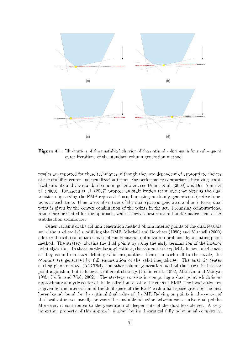
RMP (dual)

(a) (b)

(c) (d)

Figure 4.1: Illustration of the unstable behavior of the optimal solutions in four subsequentouter iterations of the standard column generation method.

results are reported for these techniques, although they are dependent of appropriate choicesof the stability center and penalization terms. For performance comparisons involving stabi-lized variants and the standard column generation, see Briant et al. (2008) and Ben Amor etal. (2009). Rousseau et al. (2007) propose an stabilization technique that obtains the dualsolutions by solving the RMP repeated times, but using randomly generated objective func-tions at each time. Then, a set of vertices of the dual space is generated and an interior dualpoint is given by the convex combination of the points in the set. Promising computationalresults are presented for the approach, which shows a better overall performance than otherstabilization techniques.

Other variants of the column generation method obtain interior points of the dual feasibleset without (directly) modifying the RMP. Mitchell and Borchers (1996) and Mitchell (2000)address the solution of two classes of combinatorial optimization problems by a cutting planemethod. The strategy obtains the dual points by using the early termination of the interiorpoint algorithm. In those particular applications, the columns are explicitly known in advance,as they come from facet de�ning valid inequalities. Hence, at each call to the oracle, thecolumns are generated by full enumeration of the valid inequalities. The analytic centercutting plane method (ACCPM) is another column generation method that uses the interiorpoint algorithm, but it follows a di�erent strategy (Go�n et al., 1992; Atkinson and Vaidya,1995; Go�n and Vial, 2002). The strategy consists in computing a dual point which is anapproximate analytic center of the localization set of to the current RMP. The localization setis given by the intersection of the dual space of the RMP with a half-space given by the bestlower bound found for the optimal dual value of the MP. Relying on points in the center ofthe localization set usually prevents the unstable behavior between consecutive dual points.Moreover, it contributes to the generation of deeper cuts of the dual feasible set. A veryimportant property of this approach is given by its theoretical fully polynomial complexity.

61

On the other hand, obtaining the analytic center at each iteration of the method may becomputationally expensive in practice, specially when many columns are added at a time(Elhedhli and Go�n, 2004). The use of stabilization terms within the ACCPM has beensuccessful, as shown in Babonneau et al. (2007).

The primal-dual column generation method is another variant which uses the interior pointalgorithm to solve the RMPs (Gondzio and Sarkissian, 1996). The method relies on dual pointsthat are well-centered in the feasible set. However, instead of recurring to the analytic centeras in the ACCPM, the primal-dual column generation method uses suboptimal solutionsthat belong to a safe neighborhood of the central path. The distance of the suboptimalsolution to optimality is dynamically adjusted in function of the column generation gap.In the �rst outer iterations, each RMP is solved with a loose tolerance, and this tolerance isdynamically reduced throughout the iterations as the gap in the column generation approacheszero. Gondzio and Sarkissian (1996) present promising computational results for a class ofnonlinear programming problems, whose linearization is solved by column generation. Usinga very similar strategy, Martinson and Tind (1999) also report a substantial reduction inthe number of outer iterations when compared to other variants of the column generationmethod. To the best of our knowledge, the primal-dual column generation method has neverbeen applied in the context of integer programming, where column generation formulationsare widely employed. Moreover, no theoretical study about the convergence of this method isavailable in the literature. We attempt to close these two gaps in the study presented in thenext section.

4.3 The primal-dual column generation method

The primal-dual column generation method is based on well-centered, non-optimal dual so-lutions of the RMPs. These dual solutions are provided by the primal-dual interior pointalgorithm at no extra cost, as this algorithm keeps the iterates close to the central path ofthe feasible set. As a result, two important features are observed in the primal-dual columngeneration method. First, the use of non-optimal solutions results in a smaller number ofinner iterations, which reduces the CPU time per outer iteration. Second, the well-centereddual points are more stable, which leads to substantial reductions in the number of outeriterations as well as in the total CPU time. In this section, we describe the foundations ofthe primal-dual column generation method and present a novel theoretical analysis regardingits convergence in a �nite number of steps.

Following the notation of Section 4.1, we consider that a given RMP is represented by(4.2) and the optimal primal-dual solution of this problem is given by (λ, u). Similarly tothe standard approach, the primal-dual column generation method starts with an initialRMP which has enough columns to avoid an unbounded solution. However, in a given outeriteration, the method obtains a suboptimal feasible solution (λ, u) of the current RMP, whichis de�ned as follows.

De�nition 4.3.1. A primal-dual feasible solution (λ, u) of the RMP is called suboptimal

solution, or ε-optimal solution, if it satis�es 0 ≤ (cT λ − bT u) ≤ ε(1 + |cT λ|), for some

tolerance ε > 0.

We denote by zRMP = cT λ the objective value corresponding to the suboptimal solution(λ, u). Since cT λ ≥ cTλ = zRMP , zRMP is a valid upper bound of the optimal value of theMP.

Once the suboptimal solution of the RMP is obtained, the oracle is called with the dualsolution u as a query point. Then, it should return either a value zSP (u) = 0, if no columns

62

could be generated from the proposed query point, or a value zSP (u) < 0, together with oneor more columns to be added to the RMP. Observe that in the second case at least one columncan always be generated, as u is dual feasible for the RMP and, hence, all columns alreadygenerated must have a nonnegative reduced cost.

Consider the value κ > 0 de�ned as (4.4). Recall this value depends on the applicationand it is typically a known parameter. According to Proposition 4.3.2, a lower bound of theoptimal value of the MP can still be obtained. It is the classical Lagrangian bound (see e.g.Briant et al., 2008; Ben Amor et al., 2009), but derived from a column generation scheme andusing a subpotimal solution.

Lemma 4.3.2. Let zSP := zSP (u) be the value of the oracle corresponding to the suboptimal

solution (λ, u). Then, κzSP + bT u ≤ z?.

Proof. Let λ? be an optimal primal solution of the MP. By using (4.1b) and zSP ≤ 0, we havethat

cTλ? − bT u =∑j∈N

cjλ?j −

∑j∈N

λ?jaTj u =

∑j∈N

λ?j (cj − aTj u) ≥∑j∈N

λ?j zSP ≥ κzSP .

Therefore, z? = cTλ? ≥ κzSP + bT u.

To provide a more stable dual information to the oracle, the suboptimal solution (λ, u)should be well-centered in the primal-dual feasible set. We say a point (λ, u) is well-centeredif it satis�es

γµ ≤ (cj − uTaj)λj ≤ (1/γ)µ, ∀j ∈ N, (4.6)

for some γ ∈ (0.1, 1], where µ = (1/|N |)(cT −uTA)λ. By imposing (4.6), we require the pointto not be too close to the boundary of the primal-dual feasible set and, hence, the oscillationof the dual solutions will be relatively small. Notice that (4.6) is a natural way of stabilizingthe dual solutions, if a primal-dual interior point method is used to solve the RMP. Indeed,the requirement in (4.6) is the same as that used in the symmetric neighborhood of the centralpath (see Chapter 2, Section 2.3).

Fig. 4.2 illustrates the behavior of well-centered, suboptimal solutions. In part (a) wehave the dual feasible set of a given RMP. The central path of the dual feasible set is givenby the curve in the middle of the feasible region (the reader should bear in mind it is just anillustration with the purpose of clarifying the theoretical background). The dashed lines closeto the central path are the bounds of the safe neighborhood of the central path. As de�ned in(4.6), the dual solutions must belong to this neighborhood. The suboptimal solution obtainedby the interior point method is represented by a (green) triangle. By using this solution, theoracle generates a new column to be added to the RMP. The cut corresponding to this columnis represent by the (blue) dashed line in part (b). Notice it is a much deeper cut than theone that would be generated by using the optimal dual solution (see Fig. 4.1). It results incutting-o� a larger portion of the dual feasible region. After adding the generated column tothe RMP, we obtain the dual feasible set given in part (c).

In order to obtain a suboptimal solution (λ, u), we need to set the tolerance ε whichde�nes the distance of the suboptimal solution to optimality. We propose to adjust thisparameter dynamically, based on the following observations. The tolerance ε can be loose atthe beginning of the column generation process, as a very rough approximation of the MPis known at this time. Throughout the outer iterations, this tolerance should be graduallyreduced so that it becomes tight when the gap is small. Let gap denote the column generation

63

(a) (b)

(c)

Figure 4.2: Illustration of the behavior of the well-centered, suboptimal solutions in twosubsequent outer iterations of the primal-dual column generation method.

relative gap, which is given by

gap :=cT λ− (κzSP + bT u)

1 + |cT λ|,

where zSP := zSP (u), as de�ned in Proposition 4.3.2. We propose to set ε in function of therelative gap, as follows. In a given outer iteration k, we recompute the relative gap so thatthe tolerance εk is updated as

εk := min{εmax, gapk−1/D}, (4.7)

where D > 1 is the degree of optimality that relates the tolerance εk to the relative gap atiteration k − 1. Here, we consider that D is a �xed parameter. Notice that an upper boundεmax is used so that the suboptimal solution is not too far from the optimum (e.g., εmax = 1.0).

It is important to emphasize that unlike in the standard approach, zSP = 0 does notsu�ce to terminate the column generation process. Proposition 4.3.3 shows that the gap isstill reduced in this case, and the progress of the algorithm is guaranteed.

Lemma 4.3.3. Let (λ, u) be the suboptimal solution of the RMP, found at iteration k with

tolerance εk > 0. If zSP = 0, then the new relative gap is strictly smaller than the previous

one, i.e., gapk < gapk−1.

Proof. We have that zRMP = cT λ is an upper bound of the optimal solution of the MP. Also,from Proposition 4.3.2 we obtain the lower bound bT u, since zSP = 0. Hence, the gap in thecurrent iteration is given by

gapk =cT λ− bT u1 + |cT λ|

.

Additionally, from De�nition 4.3.1, we know that gapk ≤ εk. Finally, from (4.7) and sinceD > 1, we have that εk < gapk−1 which completes the proof.

64

Algorithm 7 summarizes the above discussion. Notice that the primal-dual column gener-ation method has a simple algorithmic description, similar to the standard approach. Thus,it can be implemented in the same level of di�culty if a primal-dual interior point solver isreadily available. Notice that κ is known in advance and problem dependent. Also, the upperbound of the RMP, zRMP , may slightly increase from one iteration to another due to the useof suboptimal solutions and, hence, we store the best value found so far in UB (step 5).

Algorithm 7: The Primal-Dual Column Generation Method.Input: Initial RMP; parameters κ, εmax > 0, D > 1, δ > 0.Output: optimal solution λ.

1 Set LB = −∞, UB =∞, gap =∞, ε = 0.5;2 While (gap ≥ δ) do3 �nd a well-centered suboptimal solution (λ, u) of the RMP;4 UB = min{UB, zRMP };5 call the oracle with the query point u;6 LB = max{LB, κzSP + bT u};7 gap = (UB− LB)/(1 + |UB|);8 ε = min{εmax, gap/D};9 if (zSP < 0) then add the new columns to the RMP;10 end(while)

Since the primal-dual column generation method relies on suboptimal solutions of eachRMP, it is important to ensure that it is a valid column generation procedure, i.e., a �niteiterative process that delivers an optimal solution of the MP. Even though the optimalitytolerance ε decreases geometrically in the algorithm, there is a special case in which thesubproblem value zSP may be zero. This would cause the method to stall and, hence, thissituations requires an appropriate treatment. Fortunately, by using Proposition 4.3.3 wecan guarantee the method still converges successfully. The proof of convergence is given inProposition 4.3.4.

Theorem 4.3.4. Let z? be the optimal value of the MP. Given δ > 0, the primal-dual column

generation method converges in a �nite number of steps to a primal feasible solution λ of the

MP with objective value z that satis�es

(z − z?) < δ(1 + |z|). (4.8)

Proof. Consider an arbitrary iteration k of the primal-dual column generation method, withcorresponding suboptimal solution (λ, u). After calling the oracle, two situations may occur:

1. zSP < 0 and new columns have been generated. These columns correspond to dualconstraints of the MP that are violated by the dual point u. Since the columns areadded to the RMP, the corresponding dual constraints will not be violated in the nextiterations. Therefore, it guarantees the progress of the algorithm. Also, this case canonly happen a �nite number of times, as there are a �nite number of columns in theMP.

2. zSP = 0 and no columns have been generated. If additionally we have εk < δ, thenfrom Proposition 4.3.3 the gap in the current iteration satis�es gapk < δ, and thealgorithm terminates with the suboptimal solution (λ, u). Otherwise, we also knowfrom Proposition 4.3.3 that the gap is still reduced, and although the RMP in the nextiteration will be the same, it will be solved to a tolerance εk+1 < εk. Moreover, the gapis reduced by a factor of 1/D and, hence, after a �nite number of iterations we obtaina gap less than δ.

65

At the end of the iteration, if the current gap satis�es gapk < δ, then the algorithm terminatesand we have

zRMP − (κzSP + bT u)

1 + |zRMP |< δ.

Since κzSP + bT u ≤ z?, the inequality (4.8) is satis�ed with z = zRMP . The primal solutionλ leads to a primal feasible solution of the MP, given by λj = λj , ∀j ∈ N , and λj = 0,otherwise. If gapk ≥ δ, a new iteration is carried out and we have one of the above situationsagain.

Having presented a proof of convergence for the primal-dual column generation method, itis important to give some remarks about its implementation. First of all, it is important to relyon a state-of-the-art interior point solver. Notice that a primal-dual interior point method iswell-suited to this purpose. In fact, (standard) simplex type methods cannot straightforwardlyprovide suboptimal solutions which are well-centered in the dual space. Instead, the primaland dual solutions are always at the boundaries of their corresponding feasible sets. Besides,there is no control on the infeasibilities of the solutions before optimality is reached in asimplex method. In our implementation, each RMP is solved by the interior point solverHOPDM (Gondzio, 1995). It keeps the iterates inside a neighborhood of the central path,which has the form (4.6). Besides, the solver makes use of multiple centrality correctors incase a more strict centrality is required by the user (Gondzio, 1996; Colombo and Gondzio,2008).

An e�cient warmstarting technique is another essential feature in the primal-dual columngeneration method. Throughout the column generation iterations, closely-related problemsare solved, as the RMP in a given iteration di�ers from the RMP of the previous iterationby merely a few columns. Hence, this similarity should be exploited in order to reduce thecomputational e�ort of solving a sequence of problems. In our implementation of PDCGM,we rely on the warmstarting techniques available in the solver HOPDM (see Gondzio (1998);Gondzio and Grothey (2003, 2008)). The main idea of these methods consists of storing aclose-to-optimality and well-centered iterate when solving a given RMP. After a modi�cationis carried out on the RMP, the stored point is used as a good initial point to start from. SeeChapter 2, Section 2.3.1, for further details on warmstarting strategies for the primal-dualinterior point method.

4.4 Computational results

In this section, we present a computational study of the primal-dual column generation methodusing three classical problems from the literature. They are the cutting stock problem (CSP),the vehicle routing problem with time windows (VRPTW), and the capacitated lot sizingproblem with setup times (CLSPST). For each problem, we have implemented three di�erentcolumn generation variants. The descriptions of each variant are the following:

• Standard column generation method (SCGM): each RMP is solved to optimality by asimplex-type method to obtain an (extremal) optimal solution. We have used the bestavailable linear programming solver in the package IBM ILOG CPLEX v.12.1 (2010) toobtain such a solution. Preliminary tests with this package using the default settingsfor each solver have shown that the primal simplex method is slightly better than thedual method as the optimal basis remains primal feasible from one outer iteration toanother. The overall performance using the barrier method (with crossover) was inferiorto the other two methods.

66

• Primal-dual column generation method (PDCGM): the suboptimal solutions of eachRMP are obtained by using the interior point solver HOPDM (Gondzio, 1995), whichis able to e�ciently provide well-centered dual points.

• Analytic center cutting plane method (ACCPM): the dual point at each iteration is anapproximate analytic center of the localization set associated to the current RMP. Theimplementation was carried out on top of the open-source solver OBOE (COIN-OR,2010), a state-of-the-art implementation of the analytic center cutting plane strategywith additional stabilization terms (Babonneau et al., 2007).

For each problem and for every aforementioned column generation variant, the subprob-lems are solved with the same source-code. Also, the SCGM and the PDCGM are initializedwith the same columns and, hence, have the same initial RMP. The ACCPM requires aninitial dual point to start from, instead of a set of initial columns. After preliminary tests, wehave chosen initial dual points that led to a better performance of the method on average. Wehave used di�erent initial dual points for each problem, as will be speci�ed later. To run thetests we have used a computer with processor Intel Core 2 Duo 2.26 Ghz, 4 GB RAM, andLinux operating system. For each of the methods, we stop the column generation procedurewhen the relative gap becomes smaller than the default accuracy δ = 10−6.

The purpose of comparing the PDCGM against the SCGM is to give an idea of how muchit can be gained in overall performance in relation to the standard approach (i.e., extremedual solutions without any stabilization). Undoubtedly, it would be interesting to considerstabilized versions of the standard column generation in the computational study presentedhere. However, the lack of publicly available codes of stabilized versions discouraged us toinclude them to this computational study. For the interested reader, available comparisonsbetween standard and stabilized column generation methods are available in the literature forthe same problems we consider here (Rousseau et al., 2007; Briant et al., 2008; Ben Amor etal., 2009). The ACCPM was included in our experiments for being a strategy that also relieson an interior point method (although essentially di�erent). After extensive testing we chosewhat seems to be the best possible starting point/parameters setting for the OBOE solver. Toclarify the main di�erences regarding the three variants, Fig. 4.3 illustrates the dual solutionsused by the each of them. Two dual feasible sets are represented in the �gure. In each ofthem, the (yellow) ball represents the dual point used by the SCGM, i.e., an (extreme) optimalsolution. The (green) triangle represents the well-centered, suboptimal solution which is usedin the PDCGM. A (red) square is used to represent the approximate analytic center usedin the ACCPM. From (a), we have the dual feasible region of an RMP which has a uniqueoptimal dual solution. The dual feasible region from (b) illustrates the case with multipleoptimal dual solutions (primal degeneracy). The extreme optimal dual solution obtained bythe SCGM can be any of the (yellow) balls in the �gure, which are vertices of the region. Itis worth mentioning that we have additionally tested the performance of using the interiorpoint algorithm in a column generation method in which each RMP is solved to optimality.The results were inferior to the ones obtained by PDCGM, which shows that an appropriateuse of an interior point method is essential for its success in the column generation context.

In the problems addressed in this study, the master problem formulations are obtained byapplying the Dantzig-Wolfe decomposition (DWD) to standard integer programming formu-lations (see Appendix A). In each application, the decomposition leads to an integer MP andalso an integer (pricing) subproblem. Here, we relax the integrality of the variables in theinteger MP and then solve it by column generation, which gives a lower bound of the optimalvalue of the original formulation. To obtain an integer solution, it would be necessary tocombine the column generation with a branch-and-bound search, which is known as a branch-

67

(a) (b)

Figure 4.3: Illustration of the dual solutions used by each column generation variant.

and-price method (Barnhart et al., 1998; Lübbecke and Desrosiers, 2005). This combinationis out of the scope of this computational study, as we are concerned with the behavior of thecolumn generation variations. The use of the primal-dual column generation method withina branch-and-price methodology is addressed in Chapter 5.

4.4.1 Cutting stock problem

The one-dimensional CSP consists in determining the smallest number of stock rolls of �xedwidth W that have to be cut in order to satisfy the demands of m di�erent pieces of smallerwidths (Gilmore and Gomory, 1961, 1963). The coe�cient matrix of its standard integerprogramming formulation has a special structure which is well-suited to the application of theDWD (see Appendix A for a complete description of the formulation and its decomposition).The oracle associated to the decomposition is given by a set of n subproblems, where nis an upper bound for the total number of stock rolls. We assume the rolls have all thesame width W and hence the subproblems are identical. This feature leads to an aggregatedmaster problem with m+ 1 constraints and the oracle reduces to only one subproblem, whichcorresponds to an integer knapsack problem. If the k-best solutions of the knapsack problemare available, for a given k > 0, then up to k columns can be generated at each call to theoracle. It usually improves the performance of the column generation procedure, since moreinformation is gathered at each iteration.

To analyze the performance of the column generation variants addressed in this compu-tational study, we have initially selected 262 instances from the literature in one-dimensionalCSP (http://www.math.tu-dresden.de/~capad/). We have classi�ed these instances intotwo classes according to m, the number of pieces. Class S (small size instances) includes178 instances with dimensions ranging from 15 to 199 pieces, while class M (medium size in-stances) has 84 instances ranging from 200 to 555 pieces. In the computational experiments,the initial RMP consists of columns that are generated fromm homogeneous cutting patterns,which corresponds to selecting only one piece per pattern, as many times as possible withoutviolating the width W . In the ACCPM approach and after testing with di�erent values, wehave used the initial guess u0 = 0.5e which has provided the best results for this strategy.The knapsack problem is solved using a branch-and-bound method proposed by Leão (2009),which implementation was provided by the author. The method is able to provide the k-bestsolutions of the knapsack problem.

For each class of instances, we have tested the column generation variations using fourdi�erent values of k (1, 10, 50 and 100), the maximum number of columns added to the RMPat each outer iteration. Table 4.1 summarizes the obtained results. For each variation we havethree columns: the average number of outer iterations (Iter), the average CPU time spent in

68

the oracle (Oracle) and the average CPU time required for the column generation procedure(Total). For each k, the row All presents the average results over the 262 instances usingthe same k. The last three columns in Table 4.1 show the average total time per iteration(in seconds) and the oracle times are shown in parentheses. The time spent by the SCGMin solving the RMPs is very small in relation to the time required to solve the subproblems,regardless the size of the instances. It happens because the simplex method available in theCPLEX solver is very e�cient on solving/reoptimizing these linear programming problems.For the PDCGM and the ACCPM, the proportion of the total CPU time required to solvethe RMP and the oracle varies according to the size of the instances.

SCGM PDCGM ACCPM Total/Iter (Oracle/Iter)Time (in s) Time (in s) Time (in s)

k Class Iter Oracle Total Iter Oracle Total Iter Oracle Total SCGM PDCGM ACCPM1 S 571.8 2.0 2.6 368.9 1.9 4.8 466.2 3.0 10.5 < 0.01(< 0.01) 0.01(< 0.01) 0.02(0.01)

M 881.3 153.7 155.8 591.4 35.5 44.5 734.0 143.9 182.4 0.18(0.17) 0.08(0.06) 0.25(0.20)All 671.0 50.6 51.7 440.3 12.7 17.5 552.1 48.2 65.6 0.08(0.07) 0.04(0.03) 0.12(0.09)

10 S 149.7 0.9 1.2 102.2 0.8 2.1 253.1 2.5 26.1 0.01(0.01) 0.02(0.01) 0.10(0.01)M 251.4 75.8 77.0 158.4 15.1 18.3 368.3 82.6 148.7 0.31(0.30) 0.12(0.10) 0.40(0.22)All 182.3 24.9 25.5 120.2 5.4 7.3 290.0 28.2 65.4 0.14(0.14) 0.06(0.04) 0.23(0.10)

50 S 70.9 1.8 2.1 63.2 2.0 3.8 276.8 10.7 106.3 0.03(0.03) 0.06(0.03) 0.38(0.04)M 133.7 56.6 58.2 97.1 18.8 23.1 400.2 45.5 277.6 0.44(0.42) 0.24(0.19) 0.69(0.11)All 91.0 19.4 20.1 74.1 7.4 10.0 316.4 21.9 161.2 0.22(0.21) 0.13(0.10) 0.51(0.07)

100 S 53.7 3.8 4.2 53.9 4.6 7.3 308.4 31.2 221.8 0.08(0.07) 0.14(0.09) 0.72(0.10)M 101.0 66.3 67.8 82.3 25.4 31.5 449.4 96.4 525.2 0.67(0.66) 0.38(0.31) 1.17(0.21)All 68.8 23.9 24.6 63.0 11.3 15.1 353.6 52.1 319.1 0.36(0.35) 0.24(0.18) 0.90(0.15)

Table 4.1: Average results on the 262 CSP instances using di�erent values for k (maximumnumber of columns added to the RMP at a time).

Regardless the number of columns added at each outer iteration (k), the PDCGM has thesmallest number of iterations on average. For instances in classM , the PDCGM is on averagemore e�cient than the SCGM and the ACCPM in terms of CPU time as well. For example,if we consider k = 100, the PDCGM is 2.2 times faster than the SCGM and 16.7 times fasterthan the ACCPM in the medium size instances. We observe similar results by considering allthe instances. Indeed, the PDCGM is 1.6 times faster than the SCGM and 21.1 times fasterthan the ACCPM on average, also for k = 100. Only in the class of small instances (S), weobserve that the SCGM is more e�cient than the PDCGM and the ACCPM regarding theaverage CPU time.

The results in Table 4.1 indicate that PDCGM with k = 10 is the variant with the bestoverall performance regarding CPU time. On average, it is 2.8 and 8.9 times faster thanthe best scenarios for the SCGM (k = 50) and the ACCPM (k = 10), respectively. Thebehavior of the ACCPM is adversely a�ected by the number of columns added at a time, asthe number of iterations and the CPU time required for solving the RMPs are considerablyincreased for larger values of k. The main reason for this behavior is that the localization setmay be drastically changed from one outer iteration to another if many columns are added.Hence, �nding the new analytic center can be very expensive in this case. Another importantobservation is that the average CPU time per iteration spent in the oracle is smaller for thePDCGM and the ACCPM than for the SCGM, which is a consequence of using well-centered,stable dual solutions. Furthermore, the PDCGM seems to be able to solve the RMPs moree�ciently than the ACCPM and, hence, this variant achieved better total average CPU timesper iteration.

We further compare the performance of the three column generation variants by reportingthe results on 14 additional instances, in which m, the number of items, varies from 615 to1005. Thus, we have large restricted master problems in this experiment. Table 4.2 shows

69

the results of each column variant using k = 100. In all cases, the PDCGM is faster andrequires less iterations than the SCGM and the ACCPM, which supports the conclusion thatthe relative performance of the PDCGM is improved as the instances become larger.


Instance m Iter Oracle Total Iter Oracle Total Iter Oracle Total SCGM PDCGM ACCPMBPP_U09498 1005 548 12760.2 12946.8 293 5545.0 5678.0 762 10054.0 21253.6 23.6(23.3) 19.4(18.9) 27.9(13.2)BPP_U09513 975 518 9741.1 9903.8 267 4169.3 4276.7 779 7404.4 19362.0 19.1(18.8) 16(15.6) 24.9(9.5)BPP_U09528 945 541 9011.3 9173.2 276 4810.9 4923.6 740 6586.1 15919.8 17(16.7) 17.8(17.4) 21.5(8.9)BPP_U09543 915 506 7676.4 7797.8 263 3624.1 3723.7 723 5254.7 13448.9 15.4(15.2) 14.2(13.8) 18.6(7.3)BPP_U09558 885 482 5479.0 5585.0 265 2631.4 2730.4 683 4222.4 10860.5 11.6(11.4) 10.3(9.9) 15.9(6.2)BPP_U09573 855 473 4693.7 4771.1 230 1980.2 2054.3 672 3732.1 9793.7 10.1(9.9) 8.9(8.6) 14.6(5.6)BPP_U09588 825 467 4876.0 4950.3 247 1573.9 1649.4 658 3983.1 9376.4 10.6(10.4) 6.7(6.4) 14.2(6.1)BPP_U09603 795 465 3893.9 3961.7 237 1597.8 1668.3 627 3055.2 7503.6 8.5(8.4) 7(6.7) 12.0(4.9)BPP_U09618 765 424 2773.2 2830.4 203 1041.9 1091.6 617 2156.1 6466.7 6.7(6.5) 5.4(5.1) 10.5(3.5)BPP_U09633 735 432 2832.7 2878.1 217 912.4 969.0 595 1750.7 5307.6 6.7(6.6) 4.5(4.2) 8.9(2.9)BPP_U09648 705 424 2611.3 2659.5 209 807.9 856.8 582 1403.0 4466.2 6.3(6.2) 4.1(3.9) 7.7(2.4)BPP_U09663 675 381 2155.8 2187.4 202 613.0 654.0 534 1073.7 3324.9 5.7(5.7) 3.2(3) 6.2(2.0)BPP_U09678 645 376 1745.3 1774.6 173 387.1 417.5 542 1042.8 3395.1 4.7(4.6) 2.4(2.2) 6.3(1.9)BPP_U09693 615 384 1323.6 1347.2 165 400.6 426.8 520 875.9 2773.2 3.5(3.4) 2.6(2.4) 5.3(1.7)

Table 4.2: Results on 14 large CSP instances (with k = 100).

Finally, we extend our computational study by presenting the results obtained with 160instances from the so-called triplet and uniform sets proposed in Falkenauer (1996). Table 4.3shows the results in which 100 columns are added at each outer iteration. We have groupedthe instances in three classes: S(u, t), 80 small instances with m varying from 60 to 120;M(u, t), 120 medium instances with m between 249 and 501; and L(u, t), 20 large instanceswith m = 1000. For the last class of instances, the ACCPM was not able to solve all theinstances so we have omitted the corresponding results in the last row. The columns in Table4.3 have the same meaning as in Table 4.1. For these instances, the SCGM performs betterthan the PDCGM and the ACCPM in classes S(u, t) andM(u, t). However for large instances(L(u, t)), PDCGM outperforms the SCGM in both CPU time and number of outer iterations.


Class Iter Oracle Total Iter Oracle Total Iter Oracle Total SCGM PDCGM ACCPMS(u, t) 31.0 0.9 1.0 34.0 1.7 2.2 143.3 4.8 13.7 0.03(0.03) 0.06(0.05) 0.10(0.03)M(u, t) 150.6 259.4 263.5 110.2 396.0 405.1 383.3 443.5 1064.3 1.75(1.72) 3.68(3.59) 2.78(1.16)L(u, t) 442.7 142.1 190.5 255.3 81.4 145.7 - - - 0.43(0.32) 0.57(0.32) -(-)

Table 4.3: Average results on 220 CSP instances from triplet and uniform problem sets(using k = 100).

4.4.2 Vehicle routing problem with time windows

Consider a set of vehicles available in a depot to serve n customers with known demands.A vehicle can serve more than one customer in a route, as long as its maximum capacityis not exceeded. Each customer must be served once within a given time window. Besides,a service time is assigned for each customer. Late arrivals are not allowed and if a vehiclearrives earlier to a customer it must wait until the time window is open. We assume all thevehicles are identical and are initially at the same depot, and every route must start and�nish at this depot. The objective is to design a set of minimum cost routes in order toserve all the customers. The column generation method has been successfully used withininteger programming methodologies in the solution of the VRPTW (Desrochers et al., 1992;Kallehauge et al., 2005). In the master problem formulation adopted here, the subproblem

70

is given by a non-elementary shortest path problem with resource constraints. Similarly toCSP, an aggregated master problem is used, as we consider identical vehicles. The restrictedmaster problems have the set covering structure and its number of rows is equal to n + 1.See Appendix A for further description about the problem formulation and the associateddecomposition.

We have selected 87 VRPTW instances from the literature (http://www2.imm.dtu.dk/~jla/solomon.html), which were originally proposed by Solomon (1987). We have dividedthem in three classes: S (small size instances, n = 25), M (medium size instances, n = 50)and L (large size instances, n = 100) classes. Each class has 29 instances. The initial columnsof the RMP have been generated by n single-customer routes which correspond to assigningone vehicle per customer. In the ACCPM approach, we have considered the initial guessu0 = 100.0e which after testing various settings has proven to be the choice which gives thebest overall results for this problem. The subproblem is solved by our own implementationof the bounded bidirectional dynamic programming algorithm using state-space relaxationand identi�cation of unreachable nodes (Feillet et al., 2004; Righini and Salani, 2008). Theimplemented solver is able to provide the k-best solutions of the subproblem.

Table 4.4 presents the performance of the three column generation variants when solvingthe master problem formulation of the VRPTW. Column k denotes the maximum number ofcolumns added to the RMP at each outer iteration. For each column generation variant wehave: the number of outer iterations (Iter),the average CPU time to solve the subproblems(Oracle) and the average total CPU time required for the column generation (Total). For eachvalue of k, the last row (All) shows the average results over the 87 instances using the samevalue of k. In the last three columns, the table shows the average Total and Oracle times periteration.


k Class Iter Oracle Total Iter Oracle Total Iter Oracle Total SCGM PDCGM ACCPM1 S 99.9 0.8 0.8 48.7 0.4 0.5 106.6 0.4 0.6 0.01(0.01) 0.01(0.01) 0.01(< 0.01)

M 279.6 20.0 20.1 101.3 6.1 6.3 162.4 7.5 7.8 0.07(0.07) 0.06(0.06) 0.05(0.05)L 797.8 469.7 470.4 213.7 127.8 128.6 292.2 163.4 164.8 0.59(0.59) 0.60(0.60) 0.56(0.56)All 392.4 163.5 163.8 121.3 44.8 45.1 187.1 57.1 57.8 0.42(0.42) 0.37(0.37) 0.31(0.31)

10 S 26.2 0.3 0.3 22.3 0.2 0.2 93.6 0.4 0.5 0.01(0.01) 0.01(0.01) 0.01(< 0.01)M 66.7 6.1 6.2 37.7 2.4 2.6 122.0 5.4 5.7 0.09(0.09) 0.07(0.06) 0.05(0.04)L 188.2 113.5 114.1 72.6 41.0 41.6 170.6 90.9 92.1 0.61(0.60) 0.57(0.56) 0.54(0.53)All 93.7 40.0 40.2 44.2 14.5 14.8 128.7 32.2 32.8 0.43(0.43) 0.33(0.33) 0.25(0.25)

50 S 14.4 0.2 0.2 18.1 0.1 0.2 92.2 0.4 0.5 0.01(0.01) 0.01(0.01) 0.01(< 0.01)M 33.1 3.5 3.5 26.4 1.6 1.8 120.0 5.3 5.7 0.11(0.11) 0.07(0.06) 0.05(0.04)L 88.0 54.9 55.5 48.6 26.0 27.0 165.2 85.8 87.8 0.63(0.62) 0.56(0.53) 0.53(0.52)All 45.2 19.5 19.7 31.0 9.3 9.7 125.8 30.5 31.3 0.44(0.43) 0.31(0.30) 0.25(0.24)

100 S 12.2 0.2 0.2 16.7 0.1 0.2 92.3 0.4 0.6 0.02(0.02) 0.01(0.01) 0.01(< 0.01)M 26.0 2.9 3.0 23.2 1.4 1.7 119.7 5.4 5.8 0.12(0.11) 0.07(0.06) 0.05(0.05)L 65.4 41.7 42.4 37.9 20.3 21.5 166.0 84.5 87.5 0.65(0.64) 0.57(0.54) 0.53(0.51)All 34.5 14.9 15.2 25.9 7.3 7.8 126.0 30.1 31.3 0.44(0.43) 0.3(0.28) 0.25(0.24)

200 S 9.8 0.1 0.2 16.1 0.1 0.3 92.4 0.4 0.6 0.02(0.01) 0.02(0.01) 0.01(< 0.01)M 20.8 2.3 2.4 21.1 1.2 1.7 120.9 5.3 6.0 0.12(0.11) 0.08(0.06) 0.05(0.04)L 50.1 33.1 33.9 32.4 16.9 18.7 167.4 82.1 89.2 0.68(0.66) 0.58(0.52) 0.53(0.49)All 26.9 11.9 12.1 23.2 6.1 6.9 126.9 29.3 31.9 0.45(0.44) 0.30(0.26) 0.25(0.23)

300 S 9.4 0.1 0.1 15.8 0.1 0.3 93.3 0.4 0.6 0.01(0.01) 0.02(0.01) 0.01(< 0.01)M 18.0 2.1 2.2 20.4 1.2 1.8 121.1 5.2 6.1 0.12(0.12) 0.09(0.06) 0.05(0.04)L 42.6 28.7 29.7 31.5 16.2 18.8 168.7 79.4 89.9 0.70(0.67) 0.60(0.51) 0.53(0.47)All 23.3 10.3 10.7 22.6 5.8 7.0 127.7 28.3 32.2 0.46(0.44) 0.31(0.26) 0.25(0.22)

Table 4.4: Average results on 87 VRPTW instances adding at most k columns at a time.

In all the classes, the PDCGM shows the best average performance regarding the numberof iterations and total CPU time. When the size of the instances increases, the di�erencebetween the SCGM and the other two methods increases as well, with the SCGM being the

71

one which shows the worst overall performance. For k = 1, the PDCGM is on average 3.7and 1.3 times faster than the SCGM and the ACCPM, respectively. For larger values of k,the SCGM and the PDCGM have a similar overall performance in the class of small instances(S). But, if we take into account classes M and L, the PDCGM seems to be consistentlymore e�cient than the other two approaches in both, number of outer iterations and totalCPU time, for any k. The same conclusion is obtained considering all the 87 instances. Forall the strategies and values of k, the PDCGM with k = 200 is the most e�cient settingon average. This variant is 1.6 and 4.5 times faster than the best results obtained with theSCGM (k = 300) and the ACCPM (k = 100), respectively.

The results in Table 4.4 indicate that the well-centered dual points provided by the PD-CGM and the ACCPM lead to smaller average oracle CPU times per iteration when comparedto the SCGM. Di�erently from what was observed on the CSP results, the CPU time requiredfor solving the RMPs is very small not only for the SCGM, but also for the PDCGM andthe ACCPM. The ACCPM achieved now the best results regarding the total CPU times periteration, as it can e�ciently solve the RMPs in this case, even if up to 300 columns areadded at each call to the oracle. The only drawback of this strategy was the (relatively) largenumber of outer iterations.

We have tested the three column generation methods in more challenging instances, whichwere proposed by Homberger and Gehring (2005). This set of instances includes problemswith 200, 400 and 600 customers, so larger RMPs are obtained with them. Table 4.5 showsthe results of this additional experiment, in which up to 300 columns are added to the RMPat each outer iteration. Column n denotes the number of customers per instance while theremaining columns have the same meaning as in Table 4.4. For all instances, the PDCGMrequires less CPU time and fewer iterations when compared with the SCGM and the ACCPM.For the most di�cult instance, namely RC1_6_1, the PDCGM is 2.1 and 6.4 times fasterthan the SCGM and the ACCPM, respectively. In terms of time per iteration, the threestrategies behave similarly, in general.


Instance n Iter Oracle Total Iter Oracle Total Iter Oracle Total SCGM PDCGM ACCPMR1_2_1 200 57 36.4 42.7 45 26.0 34.2 423 191.5 201.9 0.7(0.6) 0.8(0.6) 0.5(0.5)C1_2_1 200 85 32.5 41.0 29 12.6 15.2 169 71.6 81.6 0.5(0.4) 0.5(0.4) 0.5(0.4)RC1_2_1 200 67 105.3 109.9 57 76.8 88.4 385 566.6 607.1 1.6(1.6) 1.6(1.3) 1.6(1.5)R1_4_1 400 131 793.3 865.2 84 596.1 640.5 636 2994.5 3075.6 6.6(6.1) 7.6(7.1) 4.8(4.7)C1_4_1 400 137 453.2 551.9 53 171.4 185.7 272 885.8 908.6 4.0(3.3) 3.5(3.2) 3.3(3.3)RC1_4_1 400 189 2706.0 2788.8 113 1359.8 1436.1 521 6547.6 6649.4 14.8(14.3) 12.7(12) 12.8(12.6)R1_6_1 600 222 7226.1 7558.4 118 4142.1 4259.9 897 25599.4 25870.2 34.0(32.6) 36.1(35.1) 28.8(28.5)C1_6_1 600 183 1920.8 2334.7 48 495.7 510.2 482 5114.7 5172.9 12.8(10.5) 10.6(10.3) 10.7(10.6)RC1_6_1 600 258 18701.4 18972.3 150 8676.8 8844.3 923 56177.4 56683.3 73.5(72.5) 59.0(57.8) 61.4(60.9)

Table 4.5: Results on 9 large VRPTW instances adding 300 columns at a time.

4.4.3 Capacitated Lot-Sizing Problem with Setup Times

Consider m items which must be processed by a single machine in n time periods. Theobjective is to minimize the total cost of producing, holding and setting up the machine inorder to satisfy the demands of each item at each time period. Processing and setup timesare associated to the manufacturing of each item and the machine has a limited capacity.This problem is known as the capacitated lot sizing problem with setup times (CLSPST) (seeTrigeiro et al., 1989; Jans and Degraeve, 2004). A detailed description of formulation andthe decomposition regarding this problem can be found in Appendix A. Each subproblemis a single-item lot sizing problem with modi�ed production and setup costs, and without

72

SCGM PDCGM ACCPM* Total/Iter (Oracle/Iter)Time (in s) Time (in s) Time (in s)

Class Inst Iter Oracle Total Iter Oracle Total Iter Oracle Total SCGM PDCGM ACCPME 58 38.1 0.7 0.7 29.7 0.5 0.9 38.3 0.7 0.8 0.02(0.02) 0.03(0.02) 0.02(0.02)F 70 33.4 0.6 0.6 28.0 0.5 0.8 40.4 0.7 0.9 0.02(0.02) 0.03(0.02) 0.02(0.02)W 12 66.4 1.2 1.2 55.3 1.0 1.8 48.6 0.8 1.1 0.02(0.02) 0.03(0.02) 0.02(0.02)G 71 44.8 6.6 6.6 32.4 3.9 4.7 43.2 5.2 5.6 0.15(0.15) 0.15(0.12) 0.13(0.12)X1 180 47.5 4.2 4.2 28.8 2.4 3.0 35.2 3.0 3.3 0.09(0.09) 0.10(0.08) 0.09(0.09)X2 180 42.6 7.4 7.5 20.5 3.5 3.9 27.4 4.6 5.0 0.18(0.17) 0.19(0.17) 0.18(0.17)X3 180 48.9 12.7 12.8 18.7 4.7 5.2 24.3 6.1 6.7 0.26(0.26) 0.28(0.25) 0.28(0.25)All 751 44.7 6.6 6.6 25.1 3.0 3.5 32.4 3.9 4.3 0.15(0.15) 0.14(0.12) 0.13(0.12)* A subset of 7 instances could not be solved by the ACCPM using the default accuracy level, δ = 10−6 (4 fromclass X2 and 3 from class X3). To overcome this, we have used δ = 10−5 for solving those instances.

Table 4.6: Average results on 751 CLSPST instances.

capacity constraints. Hence, it can be solved by the Wagner-Whitin algorithm (Wagner andWhitin, 1958). Unlike the other two applications, the oracle in the CLSPST consists of mdi�erent subproblems and the master problem has a disaggregated formulation. As a result,the master problem has n + m rows and up to m columns may be generated at each outeriteration, one from each subproblem.

We have selected 751 CLSPST instances proposed by Trigeiro et al. (1989) to test theaforementioned column generation variants. The SCGM and the PDCGM approaches areinitialized using a single-column Big-M technique. The coe�cients of this column are setto 0 in the capacity constraints and set to 1 in the convexity constraints. In the ACCPMapproach, after several settings, we have chosen u0 = 10.0e as the initial dual point. Thesubproblems are solved using our own implementation of the Wagner-Whitin algorithm.

For each column generation strategy, we found that the 751 instances were solved in lessthan 100 seconds. The majority of them were solved in less than 0.1 seconds. From theseresults, no meaningful comparisons and conclusions can be derived, so we have modi�ed theinstances in order to challenge the column generation approaches. For each instance and foreach item we have replicated their demands 5 times and divided the capacity, processing time,setup time and costs by the same factor. Also, we have increased the capacity by 10%. Notethat we have increased the size of the problems in time periods but not in items, so all instancesremain feasible. In Table 4.6, we show a summary of our �ndings using the modi�ed instances.We have grouped the instances into 7 di�erent classes. Small size instances are included inclasses E,F andW , while classes G,X1, X2 and X3 contain medium size instances. For eachclass and strategy we present: the number of outer iterations (Iter), the average CPU timeto solve the subproblems (Oracle) and the average total CPU time required for the columngeneration (Total). The last row (All) shows the average results considering the 751 modi�edinstances. Additionally to our usual notation, we have included the number of instances perclass (Inst).

From Table 4.6, we observe that the column generation variants have di�erent perfor-mances for the small instances (classes E,F and W ). On average, each variant requires lessthan 2 seconds to solve an instance from these classes. If we consider the total CPU time,the SCGM is slightly better for classes E and F , and the ACCPM outperforms the othertwo strategies only in class W . If we look at the oracle times, we will observe that for smallinstances the ACCPM and the PDCGM outperform the SCGM due to the reduction in thenumber of outer iterations. Now, if we observe the performance in classes containing largeinstances (G, X1, X2 and X3), the PDCGM outperforms the other two strategies, on aver-age. Furthermore, for the 751 instances (All), the PDCGM has the smallest average numberof outer iterations and total CPU time.

73


r Iter Oracle Total Iter Oracle Total Iter Oracle Total SCGM PDCGM ACCPM5 27.5 4.7 4.7 11.5 1.5 1.6 22.5 3.1 3.2 0.17(0.17) 0.14(0.13) 0.14(0.14)10 32.0 62.7 62.7 15.6 20.4 21.0 29.5 49.1 49.5 1.96(1.96) 1.35(1.31) 1.68(1.66)15 38.4 308.8 308.8 20.0 103.8 106.2 36.4 273.2 274.3 8.04(8.04) 5.31(5.19) 7.54(7.51)20 45.5 975.6 975.8 25.9 350.5 358.4 42.4 938.7 941.0 21.45(21.44) 13.84(13.53) 22.19(22.14)All 35.8 337.9 338.0 18.3 119.0 121.8 32.7 316.0 317.0 9.44(9.44) 6.66(6.50) 9.69(9.66)

Table 4.7: Average results on 44 CLSPST large instances.

In addition to the previous experiment, we have run the methods on a set with largerinstances. We have select 11 challenging instances from sets G, X2 and X3, namely G30, G53,G57, X21117A, X21117B, X21118A, X21118B, X31117A, X31117B, X31118A, X31118B.These instances have been replicated 5, 10, 15 and 20 times following the same proceduredescribed above. The summary of our �ndings are presented in Table 4.7, where column rdenotes the factor used to replicate the selected instances. From the results, we see that forevery choice of r, the PDCGM requires fewer outer iterations and less CPU time on average,when compared with the ACCPM and the SCGM. Considering the 44 instances (11 instancesand 4 values for r), the PDCGM is 2.8 and 2.6 times faster than the SCGM and the ACCPM,respectively. If we consider the average CPU time per iteration, then the PDCGM is the moste�cient among the variants, while the SCGM and the ACCPM have very similar times periteration.

4.4.4 Additional computational results in the literature

In Briant et al. (2008), the authors present a comprehensive computational study comparingthe standard column generation against the bundle method, a stabilized cutting plane methodwhich uses quadratic stabilization terms. A set of �ve di�erent applications were used in thecomputational experiments, including the CSP and the CLSPST (MILS problem in theirpaper). Regarding the CSP, the results indicate that using the bundle stabilization mayslightly reduce the number of iterations at the cost of worsening CPU times. In the resultsobtained for the CLSPST, the authors report that the bundle method behaves poorly in termsof both, CPU times and number of iterations, when compared with the standard columngeneration.

Rousseau et al. (2007) propose an interior point column generation technique in which thedual solutions are convex combinations of extreme dual points of the RMP. To analyze thecomputational performance of their approach, they have used the set of VRPTW Solomon'sinstances with n = 100. Only the results of 22 out of 29 instances were presented by the au-thors. Their comparison involved the implementations of the standard column generation aswell as a stabilized version called BoxPen technique (du Merle et al., 1999). Since a di�erentsubproblem solver has been used in their computational experiments, it would not be appro-priate to make a straightforward comparison of the �gures presented in their tables with thosepresented in Table 4.4. Hence, we consider the gain obtained by each approach in relationto the standard column generation. According to their results, a well-tuned implementationof the BoxPen stabilization reduces the number of outer iterations by 16%, on average, whilethe total di�erence regarding CPU times is negligible. The interior point column generationtechnique proposed by the authors showed a better performance than the BoxPen stabiliza-tion, being 1.38 times faster than the standard column generation technique. For the sameset of instances, the PDCGM is around 2 times faster than the SCGM on average (k = 100).

74


In this chapter, we have presented new developments in theory and applications of the primal-dual column generation method (PDCGM). The method relies on the primal-dual interiorpoint method to obtain non-optimal, well-centered solutions of the RMPs. Theoretical sup-port is given to show that the PDCGM converges to an optimum of the master problem,even though non-optimal dual solutions are used. Also, computational experiments show thatthe method is competitive when compared against the standard column generation method(SCGM) and the analytic center cutting plane method (ACCPM). The experiments werebased on linear relaxations of integer master problems formulations of three widely studiedinteger programming problems, namely the cutting stock problem (CSP), the vehicle routingproblem with time windows (VRPTW) and the capacitated lot sizing problem with setuptimes (CLSPST). Di�erent types of master problem formulations are used on these applica-tions: an aggregated master problem in the CSP, an aggregated master problem with a setcovering structure in the VRPTW, and a disaggregated master problem in the CLSPST. Ad-ditionally, we have tested the addition of di�erent numbers of columns at each outer iteration,which typically a�ects the behavior of the methods.

By analyzing the computational results, we conclude that the PDCGM achieves the bestoverall performance when compared to the SCGM and the ACCPM. Although the SCGM isusually the most e�cient for the small instances, we have observed that the relative perfor-mance of the PDCGM improves when larger instances are considered. The comparison of thePDCGM against the SCGM gives an idea of how much can be gained by using non-optimal,well-centered dual solutions provided by a primal-dual interior point method. One importantcharacteristic of the PDCGM is that no speci�c tuning was necessary for each application,while the success of using a stabilization technique for the SCGM and the ACCPM some-times strongly depends on the appropriate choice of parameters for a speci�c application.The natural stabilization available in the PDCGM due to the use of well-centered interiorpoint solutions is a very attractive feature of this column generation approach.

Several avenues are available for further studies involving the primal-dual column gener-ation technique. One of them is to compare the performance of the PDCGM with advancedcolumn generation variants such as generalized bundle methods and the volume algorithm(Frangioni, 2002; Barahona and Anbil, 2000). Furthermore, since the PDCGM relies on aninterior point method, the investigation of new e�ective warmstarting strategies applicable inthis context is essential for the success of the framework. In the next chapter, we address theuse of the primal-dual column generation method within a branch-price-and-cut framework.

75

Chapter 5

Using the primal-dual interior

point algorithm within the

branch-price-and-cut method

* A compact version of this chapter has been accepted for publication in the journal Com-

puters & Operations Research (see Munari and Gondzio, 2013).

The branch-price-and-cut method has been widely used for solving integer programmingmodels in which a special structure can be identi�ed in the coe�cient matrix. This structureis exploited by a reformulation technique, e.g. the Dantzig-Wolfe decomposition, that usuallyleads to a formulation with a stronger linear relaxation when compared with the linear relax-ation of the original model. By using this stronger formulation within a branch-and-boundtree, we obtain the branch-and-price method. Since the reformulation may have a huge num-ber of variables, the column generation algorithm is used to solve the linear relaxation ateach node of the tree. For this reason, the branch-and-price method is also known as integerprogramming column generation. In some cases, valid inequalities should also be added to thereformulated model to get even better bounds from the linear relaxations with the aim of im-proving the branch-and-bound search, which leads to the branch-price-and-cut method. Forcomprehensive surveys on these methods, see Barnhart et al. (1998); Lübbecke and Desrosiers(2005); Vanderbeck and Wolsey (2010).

In the vast majority of branch-price-and-cut implementations presented in the literature,a simplex-type method is used to solve the linear programming problems at each node. Hence,the generation of columns and valid inequalities are typically based on optimal solutions whichare extreme points of the problem feasible set. As it was discussed in Chapter 4, optimaldual solutions adversely a�ect the performance of the column generation method, as theyoscillate sharply in subsequent iterations of the method. To overcome this unstable behavior,more e�cient variants of the column generation method use non-optimal dual solutions. Thegeneration of valid inequalities by using non-optimal primal solutions has shown to be moree�ective as well, since deeper cuts are obtained and a smaller number of them are usuallyneeded.

Although very successful in many other �elds related to linear programming, interior pointmethods do not seem to have made a big impact in the integer programming context. It isprobably because the standard integer programming methodologies were originally proposed

77

at a time when the simplex method was the only e�cient algorithm available for solving linearprogramming problems and, hence, they were biased to the features available in this method.Moreover, until a few years ago, interior point methods were not able to reoptimize a problemafter carrying out modi�cations to the data as e�ciently as a simplex type method, a scenariothat has changed in the last years with the development of e�cient warmstarting techniquesfor interior point methods (see Chapter 2, Section 2.3.1). Another reason may be due toprevious unsuccessful attempts of straightforwardly replacing a simplex type method by aninterior point method. These two methods are essentially di�erent and, hence, should not beused in the same way.

In this chapter, we address the several facets of using the primal-dual interior point al-gorithm within a branch-price-and-cut method. We discuss in detail how to modify the corecomponents of this method in order to exploit the advantageous features which are o�eredby the interior point algorithm. We believe it is an appropriate time for an investigation likethis, as interior point methods have achieved a mature status concerning both theory andcomputational implementations. To verify the proposed approach, we present computationalresults for well-known instances of the vehicle routing problem with time windows (VRPTW).It is a classical integer programming problem that is widely used for testing new algorithmsdue to its di�culty. It is worth mentioning that the issues related to the integration of theinterior point algorithm with the branch-price-and-cut method which we discuss here are notlimited to or specialized for the VRPTW and can be straightforwardly used in other integerprogramming applications.

The remainder of this chapter is organized as follows. In Section 2, we present a literaturereview of previous attempts of combining interior point algorithms with integer programmingmethodologies. In Section 3, we address all the issues involved in the use of the primal-dualinterior point algorithm in the branch-price-and-cut method and propose how to deal withthem. The VRPTW is described in Section 4 and the results of computational experimentswith the new approach solving the VRPTW instances are presented in Section 5. The con-clusion and potential further developments are presented in Section 6.

5.1 Interior point methods and integer programming

Starting with Karmarkar's projective algorithm (Karmarkar, 1984), interior point methodshave quickly and strongly evolved in the last few decades (Wright, 1997; Gondzio, 2012).They have been successfully applied not only to solving linear programming problems but alsoin many other areas such as quadratic, semi-de�nite, and conic programming. However, inspite of the close relationship between linear programming and integer programming, interiorpoint methods have not showed a similar impact on integer programming. In this section wepresent a literature review of di�erent attempts to use interior point methods within integerprogramming approaches that rely on linear programming relaxations. For a brief review onthe basic concepts of the primal-dial interior point algorithm, please see Chapter 2.

To the best of our knowledge, the use of the primal-dual interior point algorithm within afull branch-price-and-cut framework has never been investigated in the literature. Moreover,few attempts have been presented in the literature regarding integer programming method-ologies that are based on interior point algorithms. The �rst implementations in this sensestarted only in the beginning of the nineties, with the pioneering works by Mitchell and hiscollaborators. Mitchell and Todd (1992) combines the primal projective interior point algo-rithm with a cutting plane method and employed to solve the perfect matching problem. Theauthors propose to use early termination when solving the linear relaxations and present howto deal with several issues such as how to obtain a new iterate after adding constraints and

78

columns to a linear programming problem that has been just solved. As shown in the com-putational results, the proposed approach resulted in a reduction of the number of iterationsand the number of calls to the separation subproblem, although the CPU times were not com-petitive with a cutting plane method based on the simplex method. The authors associatethis behavior to the di�culty in calculating the projections required by the projective interiorpoint method used in their experiments, as well as to the ine�cient warm-starting strategyused after the addition of cutting planes. Indeed, a more e�cient interior point cutting planemethod was obtained a few years later, by using the primal-dual interior point method andimproved warm-starting strategies (Mitchell and Borchers, 1996; Mitchell, 2000). Accordingto the computational results presented for two integer programming applications, namely thelinear ordering problem and the max-cut problem, the interior point approach was competitivewith a cutting plane algorithm based on the simplex method.

The use of an interior point algorithm within a branch-and-bound method was �rst ex-ploited by Borchers and Mitchell (1992). The authors observed that the primal-dual interiorpoint algorithm tends to quickly �nd feasible solutions with good objective values, but thenmay spend a considerable amount of time approaching a solution accurate enough to meetthe termination criteria. In addition, the iterates tend to converge steadily to an optimalsolution and, hence, the authors propose to use an early branching strategy, which consistin not solving the node to optimality, but stopping as soon as it becomes apparent that theoptimal solution of the node includes an integer variable at a fractional value. The authorspresent preliminary computational results on a set of mixed-integer programming problems.The interior point branch-and-bound was competitive in about half of the instances in com-parison with a state-of-the-art branch-and-bound algorithm based on the simplex method. Inthe remaining instances, the latter dominates as the simplex method was signi�cantly fasterthan the primal-dual interior point method in solving the LP relaxations of these problems.The authors associate the inferior performance of the new approach to the lack of e�cientwarm-start techniques for the primal-dual interior point method, a situation that has changedsigni�cantly since then.

du Merle et al. (1999) propose the use of the analytic center cutting plane method (AC-CPM) within the branch-and-price method for solving the minimum sum-of-squares nonhier-archical clustering problem, a constrained hyperbolic program in 0-1 variables (see Aloise etal. (2012) for a recent investigation of this problem). In the ACCPM approach, an interiorpoint method is used to obtain approximate analytic centers of the localization set, which cor-responds to the dual feasible set with an additional inequality for the best bound found so far(see Go�n and Vial (2002) for further details of the method). According to the computationalresults for several fairly large data sets publicly available, the proposed combination is verypromising and allows the exact resolution of substantially larger instances than those treatedbefore. Recently, a similar combination was investigated in (Elhedhli and Go�n, 2004) forinteger programming problems. The authors show how to modify the ACCPM so that it canwarm-start after branching as well as after the addition of columns in the primal problem. Inthe computational experiments, the authors have used randomly generated instances of thebin packing problem and the capacitated facility location problem. The results show that forthe bin packing instances, the branch-and-price method using the ACCPM results in a num-ber of nodes that is comparable with the branch-and-price method using the standard columngeneration. However, the former requires on average 58% of the CPU time required by thelatter. When comparing the two methods for the facility location instances, the method usingACCPM explores less nodes and requires less computational time. Moreover, it is consistentlybetter than the method using the standard column generation in making fewer calls to thepricing subproblems and requiring less computational time per node.

79

5.2 Main issues of an interior point branch-price-and-cut method

In this section, we discuss the issues of using the primal-dual interior point algorithm withinthe branch-price-and-cut method. We address the main elements involved in this combination,namely the column generation technique, the separation and addition of valid inequalities,branching, and the use of primal heuristics. As it will be seen in the computational results,the e�ort to overcome the challenges pays o� in a number of advantageous features o�ered bythe new approach.

5.2.1 Primal-dual column generation

The column generation technique is an iterative method applied to solve a linear programmingproblem in which the coe�cient matrix has a huge number of columns, but these columnscan be generated by a rule that is known in advance. The idea is to keep only a subset ofcolumns in the coe�cient matrix, and reach an optimal solution without explicitly generatingall the columns. In the column generation literature, the linear programming problem weare interested in is called the (continuous) master problem (MP). This problem has a hugenumber of variables and hence we recur to an auxiliary problem, which has only a subset ofvariables of the MP. This auxiliary problem is called the restricted master problem (RMP).Iteratively, the columns of the MP are generated and then added to the RMP by calling theoracle (or, pricing subproblem). For a full description of the column generation method, seeChapter 4.

The standard column generation is based on optimal solutions of the dual set. However,the use of these solutions causes instability in the column generation method, due to thehigh oscillation between extreme points of consecutive outer iterations. A slow progress istypically observed, specially during the last iterations of the method. To avoid this weaknessof the method, di�erent techniques have been proposed in the literature in order to obtainnon-extremal dual points which lead to more stable strategies. In Chapter 4, we addressthe primal-dual column generation technique, which relies on the primal-dual interior pointalgorithm to solve the RMP, so that non-optimal, well-centered dual points are obtained,leading to a naturally stable strategy. Promising computational results were presented inthat chapter for this technique when solving master problems obtained from linear-relaxedreformulations of three classical integer programming problems: the cutting stock problem, thevehicle routing problem with time windows, and the capacitated lot sizing problem with setuptimes. According to the results, the primal-dual column generation technique outperforms thestandard column generation as well as the analytic center cutting plane method, consideringthe number of iterations and CPU time, on average, for all the applications used in theexperiments. Moreover, the results show that the larger the instances, the better is therelative performance of the primal-dual approach. Therefore, we conclude that an improvedcolumn generation procedure was obtained by exploiting the advantages o�ered by the interiorpoint algorithm. With this in mind, in the next section we investigate the use of the primal-dual interior point algorithm in the generation of valid inequalities, in particular for thebranch-price-and-cut method.

5.2.2 Primal-dual column and cut generation

For some applications, valid inequalities can be used to improve the bounds provided by themaster problems and consequently reduce the number of nodes in the search tree. Di�erenttypes of valid inequalities are available in the literature and their e�ectiveness usually dependson the problem. Besides, in the context of column generation, the addition of valid inequalities

80

is not a trivial task as it may drastically increase the computational cost of solving the pricingsubproblem and, hence, a good trade-o� must be achieved (Desaulniers et al., 2011; Desrosiersand Lübbecke, 2010; Poggi de Aragão and Uchoa, 2003).

Consider the RMP in a given iteration of the column generation procedure (which maybe the last one). Assume that the current primal solution is fractional so that a separation

procedure can be used to generate a subset of violated valid inequalities. By adding thesevalid inequalities to the problem, we obtain

z′RMP := min∑j∈N

cjλj , (5.1a)

s.t.∑j∈N

ajλj = b, (5.1b)

∑j∈N

hjλj ≤ d, (5.1c)

λj ≥ 0, ∀j ∈ N, (5.1d)

where d ∈ Rm′ , hj ∈ Rm′ , for all j ∈ N , and m′ > 0 is the number of valid inequalities.Let σ ∈ Rm′ be a dual solution associated to (5.1c). This dual solution must be taken intoaccount in the pricing subproblem, which can be stated as

z′SP (u, σ) := min{0; cj − uTaj − σThj | j ∈ N}, (5.2)

where hj may represent an intermediate variable vector de�ned as a function of aj or as afunction of other variables of the subproblem (see Spoorendonk (2008); Desaulniers et al.(2011) for further details). Depending on the strategy used to solve the subproblem as wellas on the type of the valid inequalities, the subproblem (5.2) may become considerably moredi�cult to solve than (4.3). In such case, this di�culty typically increases as m′ grows, so animportant concern is to keep the number of valid inequalities small.

Separation procedures are usually called at the optimal solution of the master problem,i.e., after the column generation procedure has �nished. However, as it was already mentionedin Section 5.1, calling the separation procedure before reaching optimality is likely to resultin deeper cuts, as well-centered points in the interior of the feasible set are used to generatethe valid inequalities. Besides, this strategy facilitates the warm-start when an interior pointmethod is used to solve the RMP, as discussed in Section 5.2.5. With these observationsin mind, we propose to modify the PDCGM oracle presented in the previous section sothat two operations are available. Either new columns are generated by calling the pricingsubproblem, or new constraints are generated by calling the separation subproblem. Theseparation subproblem is in charge of generating valid inequalities for the RMP, based onthe current primal (feasible) solution. A few drawbacks are associated to this early searchfor valid inequalities: (i) it may be too early to call the separation subproblem and it willonly waste time without returning any violated inequality; (ii) the search may �nd too manyvalid inequalities, as an inequality may be violated by the current iterate but not by anoptimal solution. As observed by Mitchell (2000), these disadvantages may be minimized bykeeping the iterates well-centered in the feasible set, and by using a tolerance threshold tostart generating valid inequalities, as discussed below. Furthermore, the gain of using theearly search strategy is likely to overcome these potential drawbacks.

Algorithm 8 is an extension of primal-dual column generation algorithm (see Section 4.3),which takes the generation of valid inequalities into account. The oracle procedure was mod-i�ed so that the primal solution of the RMP is also sent as a parameter to the oracle in line

81

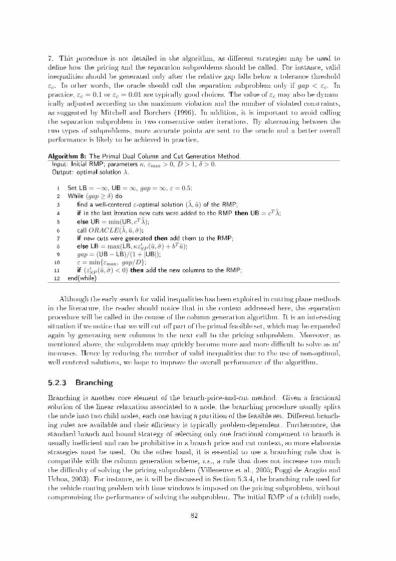
7. This procedure is not detailed in the algorithm, as di�erent strategies may be used tode�ne how the pricing and the separation subproblems should be called. For instance, validinequalities should be generated only after the relative gap falls below a tolerance thresholdεc. In other words, the oracle should call the separation subproblem only if gap < εc. Inpractice, εc = 0.1 or εc = 0.01 are typically good choices. The value of εc may also be dynam-ically adjusted according to the maximum violation and the number of violated constraints,as suggested by Mitchell and Borchers (1996). In addition, it is important to avoid callingthe separation subproblem in two consecutive outer iterations. By alternating between thetwo types of subproblems, more accurate points are sent to the oracle and a better overallperformance is likely to be achieved in practice.

Algorithm 8: The Primal-Dual Column and Cut Generation Method.Input: Initial RMP; parameters κ, εmax > 0, D > 1, δ > 0.Output: optimal solution λ.

1 Set LB = −∞, UB =∞, gap =∞, ε = 0.5;2 While (gap ≥ δ) do3 �nd a well-centered ε-optimal solution (λ, u) of the RMP;

4 if in the last iteration new cuts were added to the RMP then UB = cT λ;

5 else UB = min(UB, cT λ);

6 call ORACLE(λ, u, σ);7 if new cuts were generated then add them to the RMP;8 else LB = max(LB, κz′SP (u, σ) + bT u);9 gap = (UB− LB)/(1 + |UB|);10 ε = min{εmax, gap/D};11 if (z′SP (u, σ) < 0) then add the new columns to the RMP;12 end(while)

Although the early search for valid inequalities has been exploited in cutting plane methodsin the literature, the reader should notice that in the context addressed here, the separationprocedure will be called in the course of the column generation algorithm. It is an interestingsituation if we notice that we will cut-o� part of the primal feasible set, which may be expandedagain by generating new columns in the next call to the pricing subproblem. Moreover, asmentioned above, the subproblem may quickly become more and more di�cult to solve as m′

increases. Hence by reducing the number of valid inequalities due to the use of non-optimal,well centered solutions, we hope to improve the overall performance of the algorithm.

5.2.3 Branching

Branching is another core element of the branch-price-and-cut method. Given a fractionalsolution of the linear relaxation associated to a node, the branching procedure usually splitsthe node into two child nodes, each one having a partition of the feasible set. Di�erent branch-ing rules are available and their e�ciency is typically problem-dependent. Furthermore, thestandard branch-and-bound strategy of selecting only one fractional component to branch isusually ine�cient and can be prohibitive in a branch-price-and-cut context, so more elaboratestrategies must be used. On the other hand, it is essential to use a branching rule that iscompatible with the column generation scheme, i.e., a rule that does not increase too muchthe di�culty of solving the pricing subproblem (Villeneuve et al., 2005; Poggi de Aragão andUchoa, 2003). For instance, as it will be discussed in Section 5.3.4, the branching rule used forthe vehicle routing problem with time windows is imposed on the pricing subproblem, withoutcompromising the performance of solving the subproblem. The initial RMP of a (child) node,

82

corresponds to the last RMP of its parent node without the columns that violate the newconstraints imposed by the branching rule.

When solving the linear relaxation of a node by an interior point method, early branchingis likely to result in a better overall performance of the branch-and-bound search (Borchersand Mitchell, 1992). Similarly to what is done in the column and cut generation, the earlybranching consists in calling the branching procedure before reaching the optimality of thelinear relaxation (master problem). It is based on the fact that, when solving a standardlinear programming problem, an interior point method gets close to optimality quickly butthen may need a considerable e�ort to attain the required accuracy of the optimal solution.Indeed many components of the solution vector may reach the values which are very close tothe optimum after merely a few interior point iterations. As showed by Borchers and Mitchell(1992), it can be useful in reducing the CPU time of the overall method. However, it is notclear whether the use of early branching in combination with column and cut generation isbene�cial. In fact, the columns and cuts added in the very last iterations may be decisive forthe values of the components of an optimal solution and, hence, the early branching may bemisguided by wrong estimates of the solution values.

Here we propose to deal with the branching operation in two steps. In the �rst step, calledpreprocessing, we aim at quickly obtaining a non-optimal solution of the master problem of thecurrent node so that the �rst evidence of a potentially good branching decision is taken fromit. If the node is not eligible for pruning, then the branch is carried out and the second stepis not necessary. Otherwise, the second step is started in which the master problem is solvedto optimality. Di�erent strategies may be used to solve the problem quickly, such as settinga loose optimality tolerance εb < εc in the column and cut generation procedure, and usinga heuristic method to solve the pricing subproblem as it is usually the most time-demandingprocedure.

5.2.4 Primal heuristics

The use of quick heuristic methods is crucial in the branch-price-and-cut method, speciallyfor identifying integer feasible solutions that can be used to prune nodes. These heuristicsmay be simple generic procedures that are based on rounding the components of a fractionalsolution, but also they can be very elaborate and exploit the structure of the problem. Weare interested in general-purpose heuristics that can be used in combination with the columnand cut generation. After solving the master problem using the strategy discussed in Section5.2.2, we propose to call a primal heuristic that attempts to quickly identify an integer feasiblesolution. The use of rounding heuristics within the column generation is usually very helpful(Vanderbeck, 2000; Degraeve and Peeters, 2003), as the columns correspond to parts of aninteger solution of the original problem. Hence, by putting together a feasible subset ofthem, an integer solution is likely to be obtained. For instance, in the VRPTW a columncorresponds to a feasible route for a vehicle. By selecting a subset of routes (columns) suchthat each customer is visited exactly once by these routes, we obtain a feasible integer solution.In the approach presented in this chapter, we rely on a residual rounding heuristic, describedas follows.

Consider we have a fractional primal solution λ. The �rst step is to select up to Tcomponents of λ and round them to an integer value. Then, the columns corresponding tothe rounded components are multiplied by the new values and subtracted from b, the right-hand side vector of the RMP. The resulting problem, called residual RMP, is solved again andthe process is repeated until an integer solution is obtained or it is detected that no feasibleinteger solution can be found by the heuristic. It may happen that the residual RMP becomes

83

infeasible and hence, the column generation must be called again until a feasible solution isobtained or the infeasibility is also identi�ed by the column generation procedure. All thecolumns associated to the rounded components should be stored to eventually give rise toan integer feasible solution. Even though a modi�ed RMP is solved inside the heuristic, anycolumn that is generated during its course is also valid for the original RMP.

The rounding procedure is detailed in Algorithm 9. Ideally, the parameter T (line 5)should be very small (e.g., T = 2), but notice that this is likely to result in a large number ofiterations of the heuristic and, hence, a good compromise must be found. In line 6, di�erentstrategies could be used to select an index j. For example, j can be chosen so that λj is thevalue with the fractional part closest to 0.5. Di�erent strategies can be used in line 9 as well.Given a fractional value λj it may be rounded to its nearest integer, or rounded-up to thesmallest integer greater than or equal to its value (i.e. dλje), or still rounded-down to thelargest integer less than or equal to its value (i.e. bλjc). In all cases, the choice of the beststrategy depends on the problem we are dealing with.

Algorithm 9: Residual rounding heuristic.

Input: RMP, solution λ, tolerance ε; parameters T > 0.Output: A set of column indices T which leads to an integer solution; Fail, otherwise.

1 Set b = b, T = ∅, N = N ;2 Initialize r as the number of constraints in the RMP that are violated for λ = 0;3 while r > 0 do

4 set t = 0;5 while t < T and |N | > 0 do

6 select an index j ∈ N ;

7 if λj > 0 then

8 add j to T and increment t;

9 round λj to obtain the integer value [λj ];

10 reset the right-hand side of the RMP as b := b− [λj ]aj ;

11 solve the resulting RMP with tolerance ε to obtain a new λ;12 if the RMP became infeasible then call Algorithm 8 with δ = ε;13 if Algorithm 8 has detected the RMP is infeasible then STOP;14 end(if)15 remove j from N ;16 end(while).17 end(while).18 if r = 0 then T leads to a feasible integer solution of the RMP.

5.2.5 Warmstarting strategy

The core elements of a branch-price-and-cut method share a common feature: they typicallyinvolve the solution of a linear programming problem that is a simple modi�cation of anotherlinear programming problem that has been already solved, i.e., these problems are closely-

related. For instance, after solving an RMP in a given iteration of the column and cutgeneration procedure, the RMP to be solved in the next iteration di�ers from the previous oneby having either new columns or new constraints in the primal formulation. Any informationavailable from the solution of the previous RMP may be useful to speed up the solution ofthe new one. A technique that is able to properly exploit such information and obtain aninitial solution of the problem with bene�cial characteristics in relation to a default initialsolution is called a warmstarting technique. See Chapter 2 for a brief review on the use of thistechniques within interior point methods.

84

In the interior point branch-price-and-cut method which is proposed in this study, wefollow the warmstarting strategies by Gondzio (1998) and Gondzio and Grothey (2003). Morespeci�cally, the RMPs are solved approximately with loose accuracy requirements. Non-optimal and well-centered solutions are stored and they are later used to obtain warmstartingpoints for that new problems that are created in the primal-dual column and cut generationprocess. The solution (λ, u) sent to the oracle (see Section 5.2.2) is the same as the one storedfor constructing a warmstarting point to be used in the next outer iteration, except whenthe relative gap becomes less than a threshold value εws (e.g., εws = 10−3) which meansthe solution is too close to the boundary for leading to a good warmstart. In this particularcase, we store the iterate when for the �rst time the relative gap falls below εws and continuesolving the problem until the prede�ned optimality tolerance is reached. Before solving thenext RMP, the stored point is modi�ed to reduce the primal and dual infeasibilities, andmultiple centrality correctors (Gondzio, 1996; Colombo and Gondzio, 2008) may be appliedto improve the centrality of the warmstarting point.

5.3 The vehicle routing problem with time windows (VRPTW)

The VRPTW is a widely studied integer programming problem and covers a broad range ofreal-world applications. All the time, many companies over the world are looking for the bestroutes for delivering/collecting products to/from customers, which are usually spread in acertain neighborhood, city or even larger regions. The VRPTW can be used to model thesesituations and the e�cient solution of real-life problems is crucial for many businesses � forinteresting examples, see e.g. Braysy and Gendreau (2005); Desaulniers et al. (2010); Purezaet al. (2012); Macedo et al. (2011). Moreover, the VRPTW is important as a benchmarking fortesting new solution strategies, because it is considered a very di�cult integer programmingproblem.

5.3.1 Extended formulation

In the standard VRPTW, a set of vehicles is available in a single depot and these vehiclesmust be used to visit a set of customers C = {1, . . . ,m} in order to satisfy the demands diof each customer i ∈ C. The problem consists in determining a set of minimum cost routesfor the vehicles, satisfying the following requirements. Each customer must be visited exactlyonce and the arrival of vehicle must satisfy a time window [wai , w

bi ], i.e., the vehicle cannot

arrive after time wbi to service a customer, and it should wait until time wai in case it arrivestoo early. We denote by si the service time for customer i, and by tik the travel time fromcustomer i to another customer k. The number of customers a vehicle can serve is limited byits maximum capacity q, and the vehicle must return to the depot after visiting the customerscovered by its route. We assume the vehicles are identical and they are available in a su�cientnumber to service all the customers. The cost of a route is given by the total distance traveledby the vehicle. For a detailed description of the problem, see Appendix A.

Although a compact formulation of the VRPTW has been proposed in the literature, itslinear relaxation provides a poor bound for the value of an optimal integer solution. As aconsequence, a pure branch-and-bound strategy or even a branch-and-cut method are usuallyine�cient in practice. A better bound can be obtained by recurring to the linear relaxationof an extended formulation of the VRPTW, given by the following integer master problemwith a set-partitioning structure

min∑j∈N

cjλj (5.3a)

85

s.t.∑j∈N

ajλj = 1, (5.3b)

λj ∈ {0, 1}, ∀j ∈ N, (5.3c)

where aj = (a1j , . . . , amj)T is a column constructed from a feasible route, cj is the corre-

sponding cost to visit each customer in the route and then come back to the depot, and Nis the set of indices of all feasible routes for the problem. The coe�cients in column aj aregiven by aij = 1 if route j visits customer i and aij = 0 otherwise.

Formulation (5.3) is solved by a branch-and-price strategy. At each node, the integralityof the master variable λ is dropped and the resulting linear programming relaxation is solvedby the column generation technique. To generate columns, feasible routes are obtained bysolving an elementary shortest path problem with resource constraints (ESPPRC). Considerthat a subset of columns of the MP was obtained in previous iterations. Assume a primal-dualfeasible solution (λ, u) of the corresponding RMP is available. The dual solution is used toobtain one or more routes by solving the following subproblem:

min∑i∈C0

∑k∈C0

(cik − uk)xik (5.4a)

s.t.∑k∈C0

x0k = 1, (5.4b)

∑i∈C0

xih −∑k∈C0

xhk = 0, ∀h ∈ C, (5.4c)

∑i∈C0

xi,m+1 = 1, (5.4d)

∑i∈C

di∑k∈C0

xik ≤ q, (5.4e)

wi + si + tik −M(1− xik) ≤ wk, ∀ i, k ∈ C0, (5.4f)

wai ≤ wi ≤ wbi , ∀i ∈ C0, (5.4g)

xik ∈ {0, 1}, ∀ i, k ∈ C0, (5.4h)

where xik is a binary variable that represents whether the vehicle goes directly from customer ito customer k, wi is a real variable that gives the time customer i is visited, C0 = C∪{0,m+1}is a set of customer indices with 0 and m+ 1 representing the depot, and M is a su�cientlylarge number. Constraints (5.4b)-(5.4d) guarantee that the vehicle leaves the depot andcomes back to it in the end of the route, and also that the vehicle always leaves a customeronce it is visited. The maximum capacity of the vehicle is imposed by constraint (5.4e), andthe time windows of the customers are de�ned in constraints (5.4f)-(5.4g). Given a solution[x?ik, w

?i ]i,k∈N of problem (5.4), a new column aj is generated by setting

aij =∑k∈C0

x?ik, ∀i ∈ C.

Both an optimal solution of (5.4) and any suboptimal solution with a negative objective valuecan be used to generate a column. In practice, the ESPPRC is solved by using a dynamicprogramming strategy, as described in Section 5.3.2.

The �rst investigations concerning the use of a branch-and-price method for the VRPTWwere presented by Desrosiers et al. (1984) and Desrochers et al. (1992). Since then severalimprovements have been proposed in this context, as a result of intensive investigation inthe area (see Irnich and Desaulniers, 2005; Kallehauge et al., 2006; Feillet, 2010; Baldacci et

86

al., 2012; Rousseau et al., 2007). Branch-price-and-cut methods for the VRPTW were �rstproposed by Kohl et al. (1999) and Cook and Rich (1999), using the so-called two-path andk-path valid inequalities. Recently, the subset row inequalities and the generalized k-pathinequalities were proposed by Jepsen et al. (2008) and Desaulniers et al. (2008), respectively,leading to more powerful methods. The subset row inequalities are described in Section 5.3.3.They are used in our implementation due to their superior overall performance in practice.

5.3.2 Solving the ESPPRC

The most successful implementations for solving the ESPPRC are based on a dynamic pro-gramming algorithm. More speci�cally, it is a label-setting algorithm that was proposed byDesrochers (1988) and Beasley and Christo�des (1989), and has been signi�cantly improvedin the last years by the development of di�erent techniques, such as the identi�cation ofunreachable nodes (Feillet et al., 2004) and the bidirectional label extension with resourcebounding (Righini and Salani, 2008). Also, heuristics and meta-heuristics have been used tospeed up the implementations (Chabrier, 2006; Desaulniers et al., 2008). In this section, wedescribe the label-setting algorithm we have implemented to solve the ESPPRC. It is basedon the aforementioned publications and is presented here in order to have a self-containeddescription that covers all those contributions in a uni�ed way. The use of the subset rowinequalities introduces a slight modi�cation of the algorithm described in this section, as itwill be seen in Section 5.3.3.

Let G(V,A) be a graph de�ned by the set V of vertices associated to indices in C0 (theset of all customers plus the depot, with 0 as the source vertex and m+ 1 as the sink vertex).A vertex i ∈ V is adjacent to a vertex k ∈ V if arc (i, k) belongs to the set of arcs, denotedby A. To each arc (i, k) is associated the cost cik − uk, similarly to (5.4a). In the columngeneration context, u1, . . . , um are the dual variables associated to master constraints, andwe de�ne u0 := 0 and um+1 := 0. In the general context, they can be seen as prizes collectedwhen the respective vertex is visited and, under this point of view, cik becomes the actualcost of traversing arc (i, k).

In the label-setting algorithm, each route is obtained by iteratively extending labels whichrepresent partial paths. A label Li consists in a set of attributes that characterize the partialpath that ends in vertex i ∈ V. The attributes considered here are: c(Li), the total costalong the path; q(Li), the load accumulated along the path; t(Li), the total time spent in thepath; and vk(Li), a �ag that indicates whether vertex k is visited or not by the path, for allk ∈ V. By the feasible extension of a label, new vertices are added to the corresponding path.Here, we use the bidirectional label-setting strategy, which means that labels are generatedby forward as well as backward extension. Recall that tik denotes the travel time betweenvertices i and k, si is the service time and di is the demand of vertex i. In the forwardextension, any partial path starts at the source and it is extended until the time attributebecomes greater than or equal to T/2, where T is the maximum feasible arrival time at thesink, which is given by the largest value wbl +sl+ tl,m+1 over all l ∈ V. Given a label Fi, i ∈ V,we extend it to each vertex k ∈ V such that (i, k) ∈ A, vk(Fi) = 0, and the attribute values ofthe resulting label Fk satisfy q(Fk) ≤ q and t(Fk) ≤ wbi . The attributes of the resulting labelare given by

c(Fk) = c(Fi) + cik − uk,q(Fk) = q(Fi) + dk,

t(Fk) = max{wak, t(Fi) + si + tik},vk(Fk) = 1,

87

vl(Fk) = vl(Fi), ∀l 6= k.

The source label F0 is initialized with all attribute values equal to zero, except for v0(F0) = 1.The paths in the backward extension start at the sink and the labels are extended until thetime attribute becomes greater than or equal to T/2. Given a label Bi, i ∈ V, we extend it toeach vertex k ∈ V such that (k, i) ∈ A, vk(Bi) = 0, and the attribute values of the resultinglabel Bk satisfy q(Bk) ≤ q and t(Bk) ≤ T − wai . The extended label has the attributes

c(Bk) = c(Bi) + cik − uk,q(Bk) = q(Bi) + dk,

t(Bk) = max{T − (wbk + sk), t(Bi) + si + tik},vk(Bk) = 1,

vl(Bk) = vl(Bi), ∀l 6= k.

The sink label Bm+1 is initialized with all of the attribute values equal to zero, except forvm+1(Bm+1) = 1. In both types of extension, we keep a list of labels which are sorted inascending order by the time attribute value. At each iteration, the �rst label of the list isselected, and the label-setting stops when the list becomes empty. We try to extend a labelof vertex i to each adjacent vertex k ∈ V, following the ascending order of the cost cik − λk.It is important to check for unreachable vertices after creating a label. A vertex l ∈ V is saidunreachable for a label Lk when q(Lk) + dl > q or t(Lk) + sk + tkl > wbl . If some of theseinequalities are satis�ed we modify the visiting attribute value by setting vl(Fk) := −1, sothis information can be used later in the algorithm. Dominance rules should also be used inorder to reduce the number of labels created in the course of the algorithm. They are basedon discarding labels that are guaranteed not to lead to an optimal route. Given two labels Liand L′i associated to a vertex i ∈ V, Li does not dominate L′i if at least one of the followingconditions are satis�ed

c(Li) > c(L′i), (5.5)

q(Li) > q(L′i), (5.6)

t(Li) > t(L′i), (5.7)

vl(Li) 6= 0 and vl(L′i) = 0, for some l ∈ V. (5.8)

In such case, L′i must be further extended in the algorithm, as it can result in an optimalroute. Otherwise, L′i is dominated by Li and can be discarded without compromising theoptimal solution. After both forward and backward extensions have �nished, each forwardlabel Fi is linked to each backward label Bi, for all i ∈ V, if it results in a feasible route witha total cost c(Fi) + c(Bi) that is negative. The route with the least total cost is the optimalsolution of the ESPPRC. The remaining routes obtained by the algorithm are suboptimalsolutions that can also be used to generate columns for the restricted master problem.

The label-setting algorithm is initialized by the set of routes associated to the columnsin the restricted master problem. Up to K1 columns are used and we select those associatedto the smallest values sj , the slack dual component related to λj , for all j ∈ N . We alsouse an adaptation of the Clarke and Wright heuristic (Clarke and Wright, 1964; Braysy andGendreau, 2005) to construct initial routes that are inserted into this set. Furthermore, threeimprovement heuristics are applied upon the best paths in the set. The �rst one consists in,given a route, removing one customer at a time from it. In the second heuristic, we try toinsert one customer that is not in the route, between each two customers in the route. Thethird heuristic is given by swapping any two consecutive customers of a route. In all methods,

88

we try to improve up to K2 routes of the initial set, those with the least reduced costs. Eachheuristic is called once and a modi�ed route is inserted into the set if it has a negative reducedcost.

As proved by Dror (1994), the ESPPRC is a strongly NP-hard problem. Finding theoptimal route at each call to the oracle is computationally expensive and should be avoidedin the column generation procedure, as the optimal solution is needed only at the last outeriteration. This way, a few simpli�cations are made on the exact label-setting algorithm, sothat it becomes a relatively quick heuristic. One simpli�cation is given by imposing a limitKd on the number of vertices for which we verify conditions (5.8) in the dominance checking.Besides, a given label is extended to at most Ke adjacent vertices. Another simpli�cationconsists in setting a limitKl for the total number of labels generated by extensions. The valuesof these three parameters are dynamically chosen according to the relative gap in the columngeneration procedure. When the relative gap falls below the column generation optimalitytolerance δ, we discard these simpli�cations and call the exact label-setting algorithm.

The �rst branch-and-price implementations for the VRPTW were based on the SPPRC,a relaxation of the ESPPRC that allows the routes to be non-elementary, i.e., it allows cycles(Desrosiers et al., 1984; Desrochers et al., 1992). The advantage is that the SPPRC canbe solved in pseudo-polynomial time using a label-setting algorithm similar to the one justdescribed in this section. However, the lower bounds obtained at the end of the columngeneration procedure may be worse than those obtained when the ESPPRC is used as thepricing subproblem, which may adversely a�ect the performance of the branch-and-boundsearch. To improve those bounds, a 2-cycle elimination is proposed by Desrochers et al.(1992) and extended to k-cycle elimination by Irnich and Villeneuve (2006). Even though,the current state-of-the-art implementations suggest that using the ESPPRC as the pricingsubproblem results in a better overall performance of the branch-and-price method.

5.3.3 Valid inequalities for the VRPTW

Di�erent types of valid inequalities are available for the VRPTW. Some of them are basedon the variables of the compact formulation of the problem (Kohl et al., 1999; Cook andRich, 1999; Desaulniers et al., 2008), which do not increase the di�culty of solving the pricingsubproblem in a branch-and-price approach. Others are based on the extended formulation(Jepsen et al., 2008; Spoorendonk, 2008), which leads to tighter bounds at the cost of havinga more di�cult pricing subproblem. In our implementation, we use a valid inequality of thissecond type, namely the subset row (SR) inequality proposed by Jepsen et al. (Jepsen et al.,2008). This inequality is a Chvatal-Gomory rank-1 cut inspired by the clique and odd-holeinequalities for the set partitioning formulation. In the remainder of this section we brie�ydescribe the SR inequality and discuss the issues involved in adding the corresponding dualvariables to the subproblem.

Consider an RMP associated to problem (5.3). Given a subset S ⊂ C and a scalar θ suchthat 0 < θ ≤ |S|, the corresponding SR inequality is de�ned as

∑j∈N

⌊1

θ

∑i∈S

aij

⌋λj ≤

⌊ |S|θ

⌋, (5.9)

where N ⊂ N is the set of indices of master variables in the RMP. Such inequality is validfor any problem having the set-partitioning structure and follows from Chvatal-Gomory'sprocedure. In fact, for any subset S, if we take for each i ∈ S the master constraints (5.3b),

89

scale each one with 1/θ and add them all, the resulting inequality is

∑i∈S

1

θ

∑j∈N

aijλj ≤|S|θ.

Now, taking the �oor on both sides we obtain the SR inequality (5.9). As proved in (Jepsen etal., 2008), the separation problem of SR inequalities is NP -complete. In the same paper, theauthors suggest the choices |S| = 3 and θ = 2, as SR inequalities using other values seldomappeared in the computational experiments carried out on benchmarking instances. In thisparticular case, the SR inequality for a given subset S is given by∑

j∈NS

λj ≤ 1,

where NS ⊂ N is the subset of routes which visit at least θ = 2 customers that belongs to S.

In a given iteration of the column and cut generation algorithm presented in Section5.2.2, let (5.1) represent the associated RMP. The dual variables σ1, . . . , σm′ associated toeach valid inequality in this problem must be taken into account in the subproblem solver.It can signi�cantly increase the di�culty of solving the subproblem, in particular when thelabel-setting algorithm is used for solving the ESPPRC. To reduce these e�ects, a modi�eddominance criteria for the label-setting algorithm is proposed by Jepsen et al. (2008) anddescribed as follows. Extending the description presented in Section 5.3.2, we de�ne for anylabel Li the additional attributes rS(Li), for each set S associated to an SR inequality in thecurrent RMP. For a given set S, rS(Li) is a counter for the number of customers in S thatare visited by the partial path represented by label Li. The attribute cost of the label mustalso be modi�ed to consider the dual component σS but only if rS(Li) ≥ 2, i.e., the pathvisits at least two customers that belong to S. The cost attribute is initialized as zero ondepot vertices, and after extending Li to obtaining a label Lk, the cost is now given by theexpression

c(Lk) = c(Li) + cik − uk −∑S∈S1

σS ,

in both forward and backward extensions, where S1 = {S | k ∈ S and rS(Lk) = 2}. In thedominance criteria, the condition (5.5) is replaced by

c(Li)−∑S∈S2

σS > c(L′i),

where S2 = {S | σS < 0 and rS(Li) mod 2 > rS(L′i) mod 2}.In order to keep the number of valid inequalities small, a few requirements can be imposed

in the separation subproblem. Similarly to Desaulniers et al. (2008), we accept only theinequalities which are violated by at least a prede�ned threshold εv. These inequalities aresorted in descending order of their violation and, then, the �rst Kv inequalities are added tothe RMP. A customer is allowed to belong to at most Ks of the sets that are used to generatethe valid inequalities. Moreover, as proposed in Section 5.2.2, the separation subproblem iscalled only after the relative gap in the column and cut generation procedure falls below thethreshold value εc.

90

5.3.4 Branching on the VRPTW

Di�erent branching rules have been proposed for branch-and-price methods for solving theVRPTW. In our developments, we follow the branching scheme used by Desaulniers et al.(2008). For the completeness of the presentation, the scheme is brie�y described below.Suppose the master problem has been solved and a fractional solution λ has been obtained.This solution can be expressed in terms of the variables in the compact formulation by usingthe equalities

xik =∑j∈N

pjikλj , ∀ i, k ∈ C0

where pjik is equal to 1 if the path associated to column j visits customer i and goes directlyto customer k, and equal to 0 otherwise. Notice that in a feasible integer solution we havexik ∈ {0, 1}, for all i, k ∈ C0, as each customer can be visited only once. In the fractionalsolution, we select the most fractional component xik /∈ {0, 1} and create two child nodes. Bymost fractional, we mean the component with fractional part that is closest to 0.5. On theleft node, we modify the pricing subproblem by �xing xik = 0. In the label-setting algorithm,it is done by removing arc (i, k) from the set of arcs A. On the right node, we �x xik = 1which corresponds to removing from A every arc (i, l) such that l 6= k and l 6= m + 1, andevery arc (l, k) such that l 6= i and l 6= 0. In both branches, the initial RMP contains thecolumns in the last RMP of the parent node that satisfy the new constraint imposed on xik.

The search tree is exploited by the best-�rst strategy. Moreover, we use the two-stepprocedure described in Section 5.2.3. In the �rst step, the column and cut generation algorithmis stopped with a loose optimality tolerance εb > δ and all pricing subproblems are solved bythe heuristic label-setting algorithm, i.e., with the simpli�cations described in Section 5.3.2.In case it is not possible to branch, we go to a second phase in which the default optimalitytolerance δ is adopted and the exact label-setting algorithm is used when the relative gap fallsbelow δ.

5.4 Computational results

In this section, we present the results of computational experiments using the interior pointbranch-price-and-cut method proposed in the previous sections. For brevity we will refer toour implementation as IPBPC. We have selected a classical integer programming problemthat is widely studied in the branch-and-price literature, the vehicle routing problem withtime windows (VRPTW). Of course, having computational experiments for more classes ofproblems would be very interesting but the di�culty of implementing a branch-price-and-cutmethod led us to choose one application. Nevertheless, the VRPTW has been used in manyprevious researches as a benchmark for illustrating and testing new ideas and algorithms.Moreover, the strategies proposed in Section 5.2 are independent of the problem.

The experiments are run on the benchmarking instances proposed by Solomon (1987).These instances were de�ned about 30 years ago, but the most di�cult ones were solved onlyin the last few years. They are classi�ed according to the spatial distribution of customers:C instances follow a clustered distribution, R instances follow a random distribution, and RCinstances follow a mix of both distributions. Following Desaulniers et al. (2008), we focuson the 56 largest instances in the set, all those having 100 customers. These instances arecommonly presented in two distinct sets, namely 100-series and 200-series sets, and thosein the second set have wider time windows and larger vehicle capacity, so they are morechallenging for the pricing subproblem.

91

The IPBPC framework has been implemented in the C programming language. It relieson the primal-dual interior point method implemented in the HOPDM code (Gondzio, 1995,2012) to solve all the linear programming problems. The procedures for solving the pricingand the separation subproblems have also been implemented and they follow the descriptionspresented in Sections 5.3.2 and 5.3.3. Table 5.1 shows the default parameter settings adoptedin the experiments presented in Section 5.4.1. For each parameter in the �rst column, thesecond column gives the section in which the parameter is de�ned, and the third columnshows its default value. In Section 5.4.2 we run additional experiments to verify the impactof some of these parameter choices. The experiments were performed on a Linux PC with anIntel Core i7 2.8 GHz CPU and 8.0 GB of memory.

Parameter Section Value

δ 5.2.1 10−6

εmax 5.2.1 1.0

εc 5.2.2, 5.3.3 0.1

εb 5.2.3, 5.3.4 0.001

K1 5.3.2 100

K2 5.3.2 100

Kd 5.3.2 0, if gap > 0.130, if 0.1 ≥ gap > 0.01100, if 0.01 ≥ gap

Ke 5.3.2 30

Kl 5.3.2 3 x 104, if gap > 0.14 x 104, if 0.1 ≥ gap > 0.017 x 104, if 0.01 ≥ gap > 0.001105, if 0.001 ≥ gap

Ks 5.3.3 1

Kv 5.3.3 3

εv 5.3.3 0.05

Table 5.1: Parameter choices in the IPBPC implementation for the VRPTW

5.4.1 Best results and comparison with a simplex-based approach

Tables 5.2 and 5.3 show the results for the Solomon's instances in sets 100-series and 200-series, respectively, using the IPBPC with all the features discussed in Sections 5.2 and 5.3.In both tables, the �rst two columns show the name of the instance and the value of theoptimal solution obtained by the IPBPC, respectively. In the remaining columns are giventhe total number of generated columns, the number of generated cuts, the number of nodesin the branch-and-bound tree, the total CPU time spent on the oracle, the total CPU timespent on solving the RMPs, and the total CPU time spent on solving the instance. All theCPU times are given in seconds.

The analysis of these results reveals that the oracle dominates the computational e�ort,a usual behavior in integer programming problems. Each instance in the 100-series set wassolved to optimality in less than 2300 seconds. In the 200-series set, 5 instances could not besolved to optimality due to memory over�ow in the pricing subproblem solver called at thelast outer iteration of column generation (exact label-setting algorithm). These instances arethe same ones that could not be solved by Desaulniers et al. (2008) and, hence, it was anexpected behavior as the same strategy was used for solving the pricing subproblem in thatimplementation. Nevertheless, the value of the best integer solution found for each instance isshown in Table 5.3. For the instances solved to optimality, none of them required more than17000 seconds.

92

Instance Optimal Columns Cuts Nodes Oracle time RMP time Total time

C101 827.3 2165 0 1 0.83 0.28 1.29

C102 827.3 3105 0 1 1.45 0.50 2.20

C103 826.3 3403 0 1 2.95 0.75 3.98

C104 822.9 4280 0 1 7.61 1.29 9.21

C105 827.3 2452 0 1 0.94 0.34 1.48

C106 827.3 2882 0 1 1.21 0.42 1.87

C107 827.3 2734 0 1 1.16 0.40 1.77

C108 827.3 3182 0 1 1.95 0.62 2.84

C109 827.3 3303 0 1 2.20 0.68 3.16

RC101 1619.8 2466 35 1 1.83 1.26 3.23

RC102 1457.4 3923 84 1 7.94 5.58 13.95

RC103 1258.0 5150 130 3 75.97 16.44 94.46

RC104 1132.3 6337 214 9 2230.29 52.02 2292.06

RC105 1513.7 3060 32 1 2.71 1.52 4.40

RC106 1372.7 9896 539 61 634.69 134.59 855.87

RC107 1207.8 3877 60 1 20.60 4.37 25.30

RC108 1114.2 5019 97 1 170.36 11.96 182.71

R101 1637.7 1708 4 3 0.94 0.42 1.69

R102 1466.6 2372 0 1 1.26 0.35 1.74

R103 1208.7 3337 18 1 4.10 1.74 6.18

R104 971.5 5801 184 5 364.24 33.93 411.50

R105 1355.3 2820 43 3 3.02 2.33 6.24

R106 1234.6 3722 52 3 7.77 4.10 13.17

R107 1064.6 4671 127 3 61.03 15.06 78.09

R108 932.1 5548 165 1 391.37 24.66 416.64

R109 1146.9 7010 339 35 234.72 72.51 348.13

R110 1068.0 4506 121 3 44.38 14.46 62.04

R111 1048.7 18186 672 107 1336.66 206.39 1701.96

R112 948.6 7857 415 17 1403.98 127.79 1573.75

Total 134772 3331 269 7018.14 736.73 8120.90

Table 5.2: IPBPC results for the 100-series Solomon's instances.

It is useful to compare the performance of the IPBPC with a state-of-the-art branch-price-and-cut method for the VRPTW that uses the simplex method to solve the linearrelaxations. Such comparison allows us to verify if the use of an interior point algorithmwithin a branch-price-and-cut method is indeed worthwhile. Hence, in Tables 5.4 and 5.5we show the best results available in the literature for a simplex-based branch-price-and-cutmethod (Desaulniers et al., 2008), and a comparison with the results shown in Tables 5.2 and5.3. The simplex-based implementation uses the same type of valid inequalities as presentedin Section 5.3.3 and the pricing subproblem is solved using a procedure very similar to thatdescribed in Section 5.3.2. However, the results in Desaulniers et al. (2008) were run on adi�erent computer, namely a Linux PC with a Dual Core AMD Opteron 2.6 GHz CPU, andhence the conclusions about CPU time should be taken cautiously. The �rst few columnsin Tables 5.4 and 5.5 give the number of cuts, number of nodes and total CPU times, aspresented by Desaulniers et al. (2008). The remaining columns give the ratio between thevalues in the �rst columns and the corresponding values in Tables 5.2 and 5.3. Only theinstances that were successfully solved by both approaches are presented in the tables.

For each 100-series instance, the IPBPC generated not only a smaller (or equal) numberof valid inequalities, but also a smaller (or equal) number of nodes when compared with thesimplex-based BPC. In total, the simplex-based BPC required around 68% more valid inequal-ities and 31% more nodes. The IPBPC was about 5 times faster than the other approach,but the reader should be warned that the two approaches were run on di�erent computers(we did not have access to the proprietary code used by Desaulniers et al. (2008)). Con-

93

Instance Optimal Columns Cuts Nodes Oracle time RMP time Total time

C201 589.1 2718 0 1 5.07 1.52 7.02

C202 589.1 5766 0 1 11.25 5.66 17.37

C203 588.7 7552 0 1 29.02 10.96 40.64

C204 588.1 11451 0 1 710.92 29.63 741.33

C205 586.4 3344 0 1 5.05 2.01 7.41

C206 586.0 5346 0 1 8.30 4.48 13.22

C207 585.8 6230 0 1 13.76 6.59 20.90

C208 585.8 4884 0 1 12.17 4.91 17.49

RC201 1261.8 9009 17 3 23.58 14.75 42.27

RC202 1092.3 9648 9 1 34.43 17.34 53.15

RC203 923.7 12238 6 2 305.02 34.56 341.50

RC204 783.5*

RC205 1154.0 8250 9 1 24.68 11.37 36.69

RC206 1051.1 9430 9 1 61.51 22.00 84.27

RC207 962.9 14622 116 3 2487.92 190.59 2691.81

RC208 776.1*

R201 1143.2 8466 20 1 21.05 14.58 36.24

R202 1029.6 12461 62 9 89.49 51.79 147.21

R203 870.8 14117 18 1 295.70 44.32 342.07

R204 731.3*

R205 949.8 17262 112 13 738.09 193.86 968.18

R206 875.9 18307 81 3 2042.07 113.64 2166.28

R207 794.0 15090 9 1 5434.13 65.78 5501.94

R208 701.2*

R209 854.8 15609 97 5 1073.17 137.10 1220.33

R210 900.5 16395 126 9 16454.83 280.83 16783.85

R211 746.7*

Total 228195 691 61 29881.19 1258.28 31281.16

* The instance was not solved to optimality due to memory over�ow. This value corresponds to the

best incumbent solution that was found by the IPBPC.

Table 5.3: IPBPC results for the 200-series Solomon's instances.

cerning the results for the 200-series instances, the total number of nodes in the IPBPC wasa bit larger than the number of nodes in the simplex-based approach in this case. On theother hand, the number of valid inequalities is still smaller for every instance and there is aneven larger di�erence when compared to the number of valid inequalities generated by thesimplex-based BPC. For the instance RC203, for example, the simplex-based method gener-ated almost 8 times more valid inequalities than the IPBPC. Large di�erences are observedfor other instances as well, such as RC202 and RC206, which reveals an important advantageof the IPBPC. As discussed in Section 5.2.2, keeping the number of valid inequalities small iscrucial for the e�ciency of the subproblem solver, as the SR inequalities a�ect the structureof the subproblem. Considering the total CPU time, the IPBPC outperforms the simplex-based BPC. These results indicate that the use of the primal-dual interior point algorithmwithin the branch-price-and-cut method o�ers a signi�cant advantage over the simplex-basedapproach.

5.4.2 Impact of changes in the core components

To verify the importance of the modi�cations which we have made on the core componentsof the IPBPC, we have run some additional computational experiments with di�erent choicesof parameters. With these experiments we do not aim to have an exhaustive testing of allpossible parameter choices, but rather we want to investigate the impact of changing somekey parameters of the method to get a better understanding of the proposed strategy.

94

Simplex-based BPC Ratio

Cuts Nodes Total time Cuts Nodes Total time

C101 0 1 2 1.00 1.00 1.56

C102 0 1 8 1.00 1.00 3.63

C103 0 1 28 1.00 1.00 7.04

C104 0 1 86 1.00 1.00 9.34

C105 0 1 3 1.00 1.00 2.03

C106 0 1 4 1.00 1.00 2.13

C107 0 1 4 1.00 1.00 2.27

C108 0 1 7 1.00 1.00 2.47

C109 0 1 16 1.00 1.00 5.06

RC101 87 1 19 2.49 1.00 5.88

RC102 193 3 120 2.30 3.00 8.60

RC103 262 5 541 2.02 1.67 5.73

RC104 437 21 11773 2.04 2.33 5.14

RC105 79 1 33 2.47 1.00 7.49

RC106 755 71 3916 1.40 1.16 4.58

RC107 158 1 161 2.63 1.00 6.36

RC108 228 1 635 2.35 1.00 3.48

R101 19 15 8 4.75 5.00 4.74

R102 0 1 3 1.00 1.00 1.72

R103 53 1 20 2.94 1.00 3.24

R104 391 11 3103 2.13 2.20 7.54

R105 144 3 36 3.35 1.00 5.77

R106 144 3 87 2.77 1.00 6.61

R107 227 4 416 1.79 1.33 5.33

R108 296 1 891 1.79 1.00 2.14

R109 588 65 1127 1.73 1.86 3.24

R110 219 5 426 1.81 1.67 6.87

R111 736 111 5738 1.10 1.04 3.37

R112 574 19 16073 1.38 1.12 10.21

Total 5590 352 45284 1.68 1.31 5.58

Table 5.4: Comparison to a simplex-based BPC method (100-series Solomon's instances).

In the �rst experiment, we analyze how the early branching strategy described in Sections5.2.3 and 5.3.4 a�ects the performance of the IPBPC. In Fig. 5.1 we plot the results of solvingall the 100-series instances with di�erent choices of the parameter εb, the threshold tolerancefor �nishing the preprocessing step in the two-step branching approach. Four di�erent valuesof εb were tested: 10−3, 10−4, 10−5 and 10−6. Three plots are given in Fig. 5.1 and they show(a) the total number of valid inequalities, (b) the total number of nodes in the search tree,and (c) the total CPU time, for each choice of εb. From (a), we see that the values 10−3 and10−4 resulted in the smallest numbers of valid inequalities. From (b) and (c), we deduce thatεb = 10−3 resulted in the smallest number of nodes and the best total CPU time. The use ofεb = 10−6 in the branching strategy causes a loss of e�ciency measured in nearly doubling theCPU time when compared with using εb = 10−3. Hence, we conclude that the early branchingcontributed to the overall e�ciency of the IPBPC. Notice that a reduction in the CPU timewas expected for larger values of εb, as the column and cut generation is stopped earlier and,hence, less calls to the oracle are made. However, the reduction in the number of nodes isan interesting result and it suggests that, indeed, interior point methods have the advantageof quickly approaching the optimal solution. As a consequence of this feature, the providedsuboptimal solutions are accurate enough to be safely used in the branching procedure.

The second experiment involves the impact of the parameter εc which is used in theoracle of the column and cut generation procedure described in Section 5.2.2. Recall thatthis parameter has the following purpose: the separation subproblem is called by the oracle

95

Simplex-based BPC Ratio

Cuts Nodes Total time Cuts Nodes Total time

C201 0 1 9 1.00 1.00 1.28

C202 0 1 49 1.00 1.00 2.82

C203 0 1 122 1.00 1.00 3.00

C204 0 1 16416 1.00 1.00 22.14

C205 0 1 15 1.00 1.00 2.02

C206 0 1 24 1.00 1.00 1.82

C207 0 1 84 1.00 1.00 4.02

C208 0 1 26 1.00 1.00 1.49

RC201 55 3 92 3.24 1.00 2.18

RC202 39 1 89 4.33 1.00 1.67

RC203 47 1 324 7.83 1.00 0.95

RC205 32 1 111 3.56 1.00 3.03

RC206 73 1 344 8.11 1.00 4.08

RC207 210 5 91405 1.81 1.67 33.96

R201 52 1 78 2.60 1.00 2.15

R202 152 17 1663 2.45 1.89 11.30

R203 78 1 641 4.33 1.00 1.87

R205 345 9 6904 3.08 0.69 7.13

R206 171 1 60608 2.11 0.33 27.98

R207 24 1 11228 2.67 1.00 2.04

R209 248 3 22514 2.56 0.60 18.45

R210 266 5 400904 2.11 0.56 23.89

Total 1792 58 613650 2.59 0.97 19.62

Table 5.5: Comparison to a simplex-based BPC method (200-series Solomon's instances).Variations_sum

Page 1

10 ³⁻ 10⁻⁴ 10⁻⁵ 10⁻⁶250

260

270

280

290

300

310

320

330

(b)

Num

ber

of n

odes

10 ³⁻ 10⁻⁴ 10⁻⁵ 10⁻⁶2900

3000

3100

3200

3300

3400

3500

3600

3700

(a)

Num

ber

of v

alid

ineq

ualit

ies

Variations_sum

Page 1

10 ³⁻ 10⁻⁴ 10⁻⁵ 10⁻⁶250

260

270

280

290

300

310

320

330

(b)

Num

ber

of n

odes

10 ³⁻ 10⁻⁴ 10⁻⁵ 10⁻⁶2900

3000

3100

3200

3300

3400

3500

3600

3700

(a)

Num

ber

of v

alid

ineq

ualit

ies

Variations_sum

Page 1

10 ³⁻ 10⁻⁴ 10⁻⁵ 10⁻⁶2000

4000

6000

8000

10000

12000

14000

16000

18000

(c)

CP

U ti

me

Figure 5.1: Impact of changing the early branching threshold εb.

only after the relative gap falls bellow εc. Three di�erent values of εc were tested in thisexperiment, namely 0.1, 0.01 and 0.001. In addition, recall that after calling the separationsubproblem, up to Kv valid inequalities are added to the RMP. The default value Kv = 3is used in the IPBPC, but for a small εc it may be better to allow a larger number of validinequalities to be added to the RMP. Hence, we have run tests with Kv = 10 as well. Fig.5.2 summarizes the results that were obtained in this experiment. It has three plots with thesame meaning as those given in Fig. 5.1. Each plot shows the results for di�erent choices of εc;the continuous line corresponds to Kv = 3 while the dashed line corresponds to Kv = 10. Theanalysis of these results suggests that the best approach corresponds to calling the separationsubproblem as soon as the relative gap in the column and cut generation procedure falls below0.1. For this scenario, Kv = 3 seems to be a more appropriate choice than Kv = 10, as thelatter resulted in a larger number of generated valid inequalities and larger number of nodes.In addition, the CPU time was considerably increased. The results forKv = 10 were improvedwhen εc was reduced, but still they were inferior to the overall performance with Kv = 3.

96

Variations_sum

Page 1

10 ¹⁻ 10 ²⁻ 10 ³⁻2000

2500

3000

3500

4000

4500

5000

(a)

Num

ber

of v

alid

ineq

ualit

ies

Variations_sum

Page 1

10 ¹⁻ 10 ²⁻ 10 ³⁻0

100

200

300

400

500

600

(b)

Num

ber

of n

odes

10 ¹⁻ 10 ²⁻ 10 ³⁻2000

7000

12000

17000

22000

27000

32000

37000

(c)

CP

U ti

me

Variations_sum

Page 1

10 ¹⁻ 10 ²⁻ 10 ³⁻2000

7000

12000

17000

22000

27000

32000

37000

(c)

CP

U ti

me

Figure 5.2: Impact of changing the separation subproblem threshold εc.


In this chapter, we have addressed the use of the primal-dual interior point algorithm withinthe branch-price-and-cut method. For each core component of the method, namely the columngeneration procedure, the separation of valid inequalities (cuts) and the branching procedure,we have presented how to exploit certain advantages that are provided by the interior pointalgorithm. Two of them are particularly attractive in this context: (i) the ability to workwith well-centered solutions stabilizes the column and cut generation procedure; (ii) the use ofearly termination improves the overall e�ciency of the approach. To verify the behavior of theproposed interior point branch-price-and-cut method, we have run computational experimentson well-known instances of the vehicle routing problem with time windows, a classical integerprogramming problem. The results provide evidence that the proposed method is e�cientand outperforms the state-of-the-art standard branch-price-and-cut method which uses thesimplex method to solve the linear relaxations. We have observed considerable reductions inthe number of nodes in the search tree, in the number of generated valid inequalities and inthe CPU time to solve the instances.

The next steps regarding this investigation will involve solving di�erent integer program-ming problems by the interior point branch-price-and-cut method proposed here. The focuswill be on problems with a large-scale master problem formulation, so that a larger percent-age of CPU time is spent on solving the RMPs. Also, we intend to improve our ESPPRCimplementation by following the main ideas discussed by Baldacci et al. (2012) in order tosolve the Solomon's instances that could not be solved by the current implementation.

97

Chapter 6

Conclusion

The linear optimization methodologies have been around for more than 50 years. Even though,the research regarding these methodologies is still very active nowadays. In this thesis, wehave presented theoretical and computational developments with the aim of contributing withthe state-of-the-art in linear optimization. At the end of each chapter, we have presented theconcluding remarks regarding the addressed subjects. We now summarize the main outcomesof each chapter.

In Chapter 2, we introduced a uni�ed framework to describe simplex type methods andinterior point method in a uniform way. The description presents these methodologies by usingthe same notation and nomenclature. Hence, it allows to pointing out the main similaritiesand di�erences regarding these methods. We believe that this uni�ed framework may behelpful to the newcomers in the area, who want to learn about the main linear programmingmethodologies. Also, it may be useful to those who are already familiar with simplex typemethods, as this framework states these methods in a new perspective.

The dual simplex method for problems in the general form, which we address in Chapter 3,is a competitive variant of simplex type methods. We presented a novel theoretical descriptionfor this method, which follows the uni�ed framework that we propose in Chapter 2. Inaddition, we discussed the main computational techniques which are important to obtain ane�cient implementation of the method. We have run computational experiments with theNetlib instances, which are commonly used to benchmark linear programming solvers. Theresults indicate that dual simplex method for problems in the general form is more e�cientthan the primal simplex method for problem in the standard form. This variant was around10% faster than the dual simplex method for problems in the standard form. Therefore, thisvariant seems promising and should be further investigated. In particular, phase-I strategiesmay be used to improve the performance of the method. Also, di�erent pricing rules should bestudied, including the extension of those which are used in the standard dual simplex method.

The use of the primal-dual interior point algorithm within the column generation methodhas shown to be a successful strategy. As presented in Chapter 4, the key idea of the primal-dual column generation method is to use the interior point method to obtain suboptimalsolutions which are well-centered in the feasible set. Hence, these solutions contribute withthe stability of the column generation technique. The results of extensive computationalexperiments indicate that the primal-dual column generation has the best overall performancein relation to the standard column generation method and the analytic center cutting planemethod. The experiments were based on linear relaxations of classical integer programmingproblems, namely the cutting stock problem, the vehicle routing problem with time windowsand the capacitated lot sizing problem with setup times. These problems are described inAppendix A, in which we present the main formulations and how to decompose them by using

99

the Dantzig-Wolfe decomposition. As a future study, we plan to further verify the performanceof this variant in di�erent types of problems, specially those with large-scale formulations.Moreover, it would be interesting to extensively compare the primal-dual column generationmethod to other stabilized variants such as the bundle method and the volume algorithm.

The advantageous features that are provided by interior point algorithms are also ben-e�cial to the branch-price-and-cut method. In Chapter 5, we show how to combine thesetwo methodologies in order to improve the performance of solving integer programming prob-lems. The proposed interior point branch-price-and-cut method exploits early termination andwell-centered primal and dual solutions at the core components of the branch-price-and-cutmethod, namely the generation of columns, generation of valid inequalities, and branching.We discussed in detail how to modify each of these components e�ciently. To verify the per-formance of the proposed integration, we have presented computational experiments whichwere based on widely used instances of the vehicle routing problem. The results show that theinterior point branch-price-and-cut method is more stable than the standard branch-price-and-cut method on these instances. On average, the number of valid inequalities is considerablysmaller in the interior point approach. The CPU time is also smaller than in the standardapproach, and the proposed method is on average 20 times faster in the most di�cult classof instances. It is worth mentioning that this research was motivated by the low usage ofinterior point methods within integer programming methodologies. In fact, the vast majorityof implementations of the branch-and-price method are based on (extreme) optimal solutionswhich are obtained by simplex type methods. Therefore, one of the contributions of thisinvestigation is to show that interior point methods can and should be used in the contextof integer programming. Further studies on this topic will involve the solution of di�erentclasses of problems. Also, we plan to integrate the interior point algorithm with other integerprogramming methodologies.

In summary, we believe that we have achieved the main goal of this doctoral research,which was to propose new strategies to improve linear optimization methodologies. Thisresearch involved the study of di�erent types of theoretical subjects and computational meth-ods, which are usually treated separately in the literature. Indeed, not many publications dealwith both simplex type methods and interior point methods. Moreover, few papers deal withthe use of interior point methods within integer programming methodologies. In this study,we have put together di�erent subjects of the linear optimization �eld with the purpose ofexploiting the strength of each one and, hence, to improve the state-of-the-art methodologies.

100

Appendix A

The Dantzig-Wolfe decomposition

In this Appendix, we describe the fundamental concepts of the Dantzig-Wolfe decomposition(DWD) and how to apply it to integer programming problems. The DWD is a techniqueproposed to decompose a linear programming problem which has a special structure in thecoe�cient matrix. The original aim of this technique consisted in making large linear problemstractable as well as to speed up the solution by the simplex method (Dantzig and Wolfe,1960). Except for some classes of problems, the DWD was not advantageous for general linearprogramming problems. However, it showed to be very successful when extended to integerprogramming problems (Barnhart et al., 1998; Vanderbeck, 2000; Lübbecke and Desrosiers,2005). In this context, the focus is to provide stronger bounds when solving linear relaxationsin order to speed up a branch-and-bound search.

The purpose of this Appendix is to support the developments presented in Chapters 4 and5, as the formulations that are addressed in those chapters are obtained by using the DWD.Moreover, the description presented here may also be useful to the reader that is interested inan introduction to the DWD. As complementary readings, we suggest the excellent papers byLübbecke and Desrosiers (2005) and Vanderbeck and Wolsey (2010). The remainder sectionsin this Appendix are the following. In Section A.1, we describe the DWD for integer program-ming problems. This decomposition is equivalent to the Lagrangian relaxation, as showed inSection A.2. Finally, we illustrate the use of the DWD on three classical integer programmingproblems: the cutting stock problem (CSP), the vehicle routing problem with time windows(VRPTW), and the capacitated lot sizing problem with setup times (CLSPST).

A.1 DWD for integer programming problems

The DWD is applied to formulations with the following special structure. The coe�cientmatrix is very sparse and composed by isolated blocks of non-zeros. In addition, the matrixhas a set of rows given by linking constraints, which links most of the variables related to theblocks of non-zeros. By discarding these constraints, the blocks would be independent fromeach other. Fig. A.1 illustrates a coe�cient matrix having the described features.

Consider the following integer programming problem, which will be referred to as thecompact formulation:

min cTx, (A.1a)

s.t. Ax = b, (A.1b)

x ∈ X , (A.1c)

101

linking constraints

isolated blocks

Figure A.1: The coe�cient matrix that has the special structure which is suitable for ap-plying the DWD.

where X = {x ∈ Zn+ : Dx = d} is a discrete set, c ∈ Rn, A ∈ Rm×n, b ∈ Rm, D ∈ Rh×n,d ∈ Rh. The constraints (A.1b) are the linking constraints in the formulation. We assumethe problem is easier to solve by taking advantage of the structure of X , in particular ofthe matrix D. Hence, by applying the DWD we are likely to obtain a more advantageousformulation.

To apply the DWD to (A.1), we consider the convexi�cation approach, although alternativeapproaches can be used as well (see e.g. Vanderbeck and Wolsey, 2010). Let C = conv(X )denote the convex hull of the set X . The convex hull is the tightest polyhedron which containsall the integer points in X . As a polyhedron, it can be fully represented by all its extremepoints pq and extreme rays pr, as stated in Theorem A.1.1.

Theorem A.1.1 (Resolution theorem). Let X = {x ∈ R | Ax ≥ b} be a nonempty polyhedron

with at least one extreme point. Let [pq]q∈Q be the extreme points, and let [pr]r∈R be a complete

set of extreme rays of X, where Q and R are the respective sets of indices. Let

C =

∑q∈Q

λqpq +∑r∈R

µrpr|∑q∈Q

λq = 1, λq ≥ 0, µr ≥ 0

.

Then C = X.

Theorem A.1.1 is also known as the Representation Theorem and the Caratheodory's The-orem. Its proof can be found in several text books (see e.g. Bertsimas and Tsitsiklis, 1997;Bazaraa et al., 1990). Notice that even though we are considering equality constraints informulation (A.1), the theorem is still valid for this case, as each equality constraint can beequivalently rewritten as two inequalities.

As a consequence of Theorem A.1.1, any x ∈ C can be rewritten as a convex combinationof the extreme points and rays of C, i.e.,

x =∑q∈Q

λqpq +∑r∈R

µrpr.

By using this correspondence in problem (A.1), we obtain the equivalent formulation:

min∑q∈Q

λq(cT pq) +

∑r∈R

µr(cT pr), (A.2a)

s.t.∑q∈Q

λq(Apq) +∑r∈R

µr(Apr) = b, (A.2b)

102

∑q∈Q

λq = 1, (A.2c)

λq ≥ 0, µr ≥ 0, ∀q ∈ Q,∀r ∈ R, (A.2d)

x =∑q∈Q

λqpq +∑r∈R

µrpr, (A.2e)

x ∈ Zn+. (A.2f)

Notice that we still need to keep x ∈ Zn+ in order to guarantee the equivalence between (A.2)and (A.1). The linear relaxation of (A.2) usually leads to a lower bound that is the same as orstronger than the one obtained by the linear relaxation of (A.1). For this reason, formulation(A.2) is more advantageous than (A.1) when using a branch-and-bound approach to solve theproblem.

Let us focus now on the linear relaxation of (A.2). Since constraints (A.2f) are dropped,there is no need to keep constraints (A.2e). By denoting cj = cT pj and aj = Apj , ∀j ∈ Q and∀j ∈ R, a relaxation of the problem (A.2) is given by:

min∑q∈Q

cqλq +∑r∈R

crµr (A.3a)

s.t.∑q∈Q

aqλq +∑r∈R

arµr = b, (A.3b)

∑q∈Q

λq = 1, (A.3c)

λq ≥ 0, µr ≥ 0, ∀q ∈ Q,∀r ∈ R, (A.3d)

which is called Dantzig-Wolfe master problem. The columns of the coe�cient matrix of thisformulation, are given by linear transformations of all extreme points and extreme rays ofC. Therefore, the number of variables in the master problem is huge, typically exponential.For this reason, the column generation method is commonly used to solve this formulation(see Chapter 4). Indeed, the columns of the master problem can be generated by solving thesubproblem

zSP (u, v) := minq∈Q,r∈R{

0, cq − uTaq − v, cr − uTar},

= minx∈C{

0, (c−ATu)Tx− v},

where u ∈ Rm and v ∈ R denote the dual variables associated to constraints (A.3b) and(A.3c), respectively.

Recall we have assumed that the matrix D in set X has a special block structure. Itallows the matrix to be partitioned in several independent submatrices Dk, k = 1, . . . ,K. Asa result, the set X is represented as the Cartesian product of K independent sets. Let usde�ne X = X1 × . . .×XK , where

Xk = {xk ∈ Z|Lk|+ : Dkxk = dk}, ∀k = 1, . . . ,K,

where |Lk| is the number of variables associated to Xk, and xk is the vector containing thecomponents of x associated to Xk. For simplicity, we assume the set X is bounded and, hence,R = ∅, although the following discussion can be extended to deal with unbounded cases (seee.g. Vanderbeck and Wolsey, 2010). Following the same ideas as described so far, problem(A.3) can be rewritten as

minK∑k=1

∑q∈Qk

ckqλkq (A.4a)

103

s.t.K∑k=1

∑q∈Qk

akqλkq = b, (A.4b)

∑q∈Qk

λkq = 1, ∀k = 1, . . . ,K, (A.4c)

λkq ≥ 0, ∀q ∈ Qk, ∀k = 1, . . . ,K, (A.4d)

where the extreme points of the subset Xk are represented by each pq with q ∈ Qk. Hence, thecolumns in this formulation are given by the extreme points from K subsets. When using thecolumn generation method to solve (A.4), up to K columns can be generated at each outeriteration, one from each subproblem

zkSP (u, vk) := min{

(ck − (Ak)Tu)Txk − vk | xk ∈ Xk}, k = 1, . . . ,K,

where Ak are the columns in A associated to the variables xk, and u ∈ Rm and v ∈ RK denotethe dual variables associated to constraints (A.4b) and (A.4c), respectively.

In certain problems, the K subsets Xk are identical and hence they lead to the sameextreme points and rays. Therefore, one of them is enough to fully represent all the columnsin (A.4), and the master variables can be aggregated as

λq :=

K∑k=1

λkq . (A.5)

As a consequence, we can drop the index k from Qk and denote it simply by Q, since all Qkrepresent the same set. The same simpli�cation may be applied to the parameters ckq and

akq . Considering all these changes together, we can rewrite problem (A.4) as the followingaggregated master problem:

min∑q∈Q

cqλq (A.6a)

s.t.∑q∈Q

aqλq = b, (A.6b)

∑q∈Q

λq = K, (A.6c)

λq ≥ 0, ∀q ∈ Q. (A.6d)

The aggregation reduces the dimensions of the master problem and only one of the subprob-lems is used in a column generation method. If 0 ∈ Xk and its associated cost is zero, thenthe equality in constraint (A.6c) can be relaxed to∑

q∈Qλq ≤ K.

In addition, if K is su�ciently large, then this inequality holds strictly in the optimal solutionand, hence, (A.6c) can be dropped from the problem.

A.2 Equivalence to Lagrangian relaxation

The dual problem associated to (A.3) has the same form as the problem we obtain by ap-plying Lagrangian relaxation for integer programming to the compact formulation (A.1) (see

104

Geo�rion (1974)). To see this, we associate a vector of Lagrange multipliers u to constraints(A.1b), and use them to penalize the violation of these constraints. Recall that C denotes theconvex hull of X . We de�ne the Lagrangian subproblem as

LD(u) = minx∈Rn

{cTx− uT (Ax− b), x ∈ X

}= min

x∈Rn

{cTx− uT (Ax− b), x ∈ C

}= uT b+ min

x∈Rn

{(cT − uTA)x, x ∈ C

}.

For an arbitrary u, we obtain a lower bound for the optimal value of problem (A.1) by solvingLD(u). The best lower bound we can obtain is given by the Lagrangian dual problem

L := maxu∈Rm

LD(u).

By representing the elements of C by its extreme points pq and extreme rays pr, with q ∈ Qand r ∈ R, we can rewrite L as the following linear programming problem

max uT b+ v

s.t. uTApq + v ≤ cT pq, ∀q ∈ Q,uTApr ≤ cT pr, ∀r ∈ R,

which is the dual problem of (A.3). It shows the relationship between DWD and Lagrangianrelaxation. Furthermore, to solve this linear programming problem we typically use the Kel-ley's cutting plane method (Kelley, 1960), in which we start with subsets Q′ ∈ Q and R′ ∈ R,and then generate other constraints iteratively, by recurring to the Lagrangian subproblemLD(u). This row generation in the dual space is equivalent to the column generation in theprimal space.

A.3 Examples of applying the DWD

In this section, we describe how to decompose three classical integer programming problemsby using the DWD. The problems we address are the following: the cutting stock problem(CSP), the vehicle routing problem with time windows (VRPTW), and the capacitated lotsizing problem with setup times (CLSPST). Di�erent types of master problem formulationsare obtained for these problems: an aggregated master problem in the CSP, an aggregatedmaster problem with a set partitioning structure in the VRPTW, and a disaggregated masterproblem in the CLSPST. We also discuss for each problem how the column generation methodcan be used for solving the resulting master problem formulation.

A.3.1 Cutting stock problem

The one-dimensional CSP consists in determining the smallest number of stock rolls of widthW that have to be cut in order to satisfy the demands dj of pieces of width wj , j ∈ M ={1, 2, . . . ,m}. We assume there is an upper bound n on the number of stock rolls needed tosatisfy the demands and, hence, we associate to each roll an index in N = {1, 2, . . . , n}. Acompact formulation for the problem is given by

min∑i∈N

yi, (A.8a)

105

s.t.∑i∈N

xij ≥ dj ∀j ∈M, (A.8b)∑j∈M

wjxij ≤Wyi ∀i ∈ N, (A.8c)

yi ∈ {0, 1}, ∀i ∈ N, (A.8d)

xij ≥ 0 and integer, ∀i ∈ N, ∀j ∈M, (A.8e)

where yi = 1 if the roll i is used, and 0 otherwise. The number of times a piece of width wjis cut from roll i is denoted by xij . Constraints (A.8b) guarantee that all demands must besatis�ed, and constraints (A.8c) enforce that the sum of the widths of all pieces cut from aroll does not exceed its width W .

The coe�cient matrix of problem (A.8) has a special structure which is well-suited tothe application of the DWD. The linking constraints in this formulation are given by (A.8b).Consider the set X of all points that satisfy constraints (A.8c), (A.8d) and (A.8e). Followingthe discussion presented in Section A.1, we de�ne the subsets Xi, for each i ∈ N , which areindependent to each other and satisfy X1× . . .×Xn = X . Furthermore, we replace each Xi byits convex hull conv(Xi), which is a bounded set and hence its set of extreme points is enoughto fully describe this set. For each i ∈ N , let Pi be the set of indices of all extreme pointsof conv(Xi). These extreme points are then denoted by (yip, x

ip1, . . . , x

ipm), for each p ∈ Pi.

Following this notation, we have the master problem:

min∑i∈N

∑p∈Pi

yipλip, (A.9a)

s.t.∑i∈N

∑p∈Pi

xipjλip ≥ dj , ∀j ∈M, (A.9b)

∑p∈Pi

λip = 1, ∀i ∈ N, (A.9c)

λip ≥ 0, ∀i ∈ N, ∀p ∈ Pi. (A.9d)

Since we have assumed the stock pieces are identical, the subsets Xi are the same for everyi ∈ N and hence they will lead to the same columns (regarding the coe�cients in the linkingconstraints). This situation should be avoided by aggregating the master variables as in (A.5).The resulting aggregated master problem is

min∑p∈P

ypλp, (A.10a)

s.t.∑p∈P

xpjλp ≥ dj , ∀j ∈M, (A.10b)

λp ≥ 0, ∀p ∈ P, (A.10c)

where P represents the set of indices of all extreme points of conv(X ), with X := X1 = . . . =Xn. Also, we dropped the convexity constraint, as 0 ∈ conv(X ) and n is an inactive upperbound in the constraint

∑p∈P λp ≤ n.

Due to the large number of columns in formulation (A.9), it is typically solved by the col-umn generation method. Let u ∈ Rm be the vector of dual variables associated to constraints(A.10b). The associated oracle is given by a subproblem of the form

min yi −∑j∈M

ujxj , (A.11a)

106

s.t. (yi, x1, . . . , xm) ∈ conv(X ), (A.11b)

where u represents an arbitrary dual solution. To obtain the solution of this subproblem, we�rst solve a knapsack problem given by

max∑j∈M

ujxj , (A.12a)

s.t.∑j∈M

wjxj ≤W, (A.12b)

xj ≥ 0 and integer, ∀j ∈M. (A.12c)

Then, an optimal solution (x?1, . . . , x?m) of (A.12) is used to generate a column of (A.10) as

follows. If 1−∑

j∈M ujx?j < 0, then the column is generated by setting yp := 1 and xpj := x?j

for all j ∈M . Otherwise, we assume the solution is given by an empty pattern and, hence, thecolumn is generated by setting yp := 0 and xpj := 0 for all j ∈ M . If the k-best solutions ofthe knapsack problem are available, for a given k > 0, then up to k columns can be generatedat each call to the oracle.

A.3.2 Vehicle routing problem with time windows

Consider a �eet of vehicles V = {1, 2, . . . , v} available to service a set of customers C ={1, 2, . . . , n} with demands di, i ∈ C. We assume all the vehicles are identical and are initiallyat a same depot, and every route must start and �nish at this depot. A vehicle can servemore than one customer in a route, as long as its maximum capacity q is not exceeded. Eachcustomer i ∈ C must be visited only once and the visiting time must satisfy a time window[wai , w

bi ]. Late arrivals (after time wbi ) are not allowed and if a vehicle arrives earlier than wai ,

then it needs to wait until the window opens. In addition, a service time si is assigned toeach customer i ∈ C. The objective in the problem is to design a set of minimum cost routesso that the described requirements are satis�ed.

Let N = {0, 1, . . . , n, n+1} be a set of vertices such that vertices 0 and n+1 represent thedepot, and the remaining vertices correspond to the customers in C. The time of travellingfrom vertex i to vertex j, denoted by tij , satis�es the triangle inequality. By using thisnotation, we can formulate the VRPTW as follows:

min∑k∈V

∑i∈N

∑j∈N

cijxijk (A.13a)

s.t.∑k∈V

∑j∈N

xijk = 1, ∀i ∈ C, (A.13b)

∑i∈C

di∑j∈N

xijk ≤ q, ∀k ∈ V, (A.13c)

∑j∈N

x0jk = 1, ∀k ∈ V, (A.13d)

∑i∈N

xihk −∑j∈N

xhjk = 0, ∀h ∈ C, ∀k ∈ V, (A.13e)

∑i∈N

xi,n+1,k = 1, ∀k ∈ V, (A.13f)

wik + tij + si −Mij(1− xijk) ≤ wjk, ∀ i, j ∈ N, ∀k ∈ V, (A.13g)

wai ≤ wik ≤ wbi , ∀i ∈ N, ∀k ∈ V, (A.13h)

107

xijk ∈ {0, 1}, ∀ i, j ∈ N, ∀k ∈ V. (A.13i)

The binary variable xijk determines whether vehicle k ∈ V visits vertex i ∈ N and then goesimmediately to vertex j ∈ N . The variable wik determines the time that vehicle k ∈ V arrivesat customer i. We assume that all the parameters are non-negative integers, cij is given bythe Euclidean distance between vertices i and j, and Mij is a su�ciently large number (e.g.,Mij = max{0, wbi + tij + si − waj }). Constraints (A.13b) guarantee that each customer mustbe visited by only one vehicle. Constraints (A.13c) enforce that a vehicle cannot exceed itscapacity. Both constraints together ensure that the demand of each client has to be satis�edby only one vehicle. Moreover, constraints (A.13d) and (A.13f) enforce that each vehicle muststart and �nish its route at the depot, respectively. Constraints (A.13e) guarantee that oncea vehicle visits a customer and serves it, it must then move to another customer or end itsroute at the depot (vertex n+ 1). Constraints (A.13g) establish the relationship between thevehicle departure time from a customer and its immediate successor. Indeed, if xijk = 1 thenthe constraint becomes wik + tij ≤ wjk. Constraints (A.13h) enforce that the vehicle k servescustomer i inside the time window [wai , w

bi ]. Note that if a vehicle is not used, its route is

de�ned as (0, n+ 1).The coe�cient matrix of formulation (A.13) has a special structure that can be exploited

by the DWD, taking (A.13b) as the linking constraints. Let X be the set of all points satisfyingconstraints (A.13c) to (A.13i). We can de�ne v independent subsets Xk from X , for eachk ∈ V , such that X = X1 × . . .×Xv. We replace each Xk by its convex hull conv(Xk), whichis a bounded set and hence is fully represented by its set of extreme points. For each k ∈ V ,Pk represents the set of indices of all extreme points of conv(Xk). Following developments inSection A.1, we obtain the master problem

min∑k∈V

∑i∈N

∑j∈N

∑p∈Pk

cijxkijpλ

kp (A.14a)

s.t.∑k∈V

∑j∈N

∑p∈Pk

xkijpλkp = 1, ∀i ∈ C, (A.14b)

∑p∈Pk

λkp = 1, ∀k ∈ V, (A.14c)

λkp ≥ 0, ∀k ∈ V,∀p ∈ Pk, (A.14d)

where for a given p ∈ Pk, xkijp are the components of the corresponding extreme point of

conv(Xk), for all i, j ∈ N . We assume that all the vehicles are identical, so the subsets Xk willbe the same for every k ∈ V . This characteristic allows us to aggregate the master variablesby using the rede�nition given in (A.5). As a result, we obtain the aggregated master problem

min∑i∈N

∑j∈N

∑p∈P

cijxijpλp (A.15a)

s.t.∑j∈N

∑p∈P

xijpλp = 1, ∀i ∈ C, (A.15b)

λp ≥ 0, ∀p ∈ P, (A.15c)

where P is the set of indices of all extreme points of conv(X ), with X := X1 = . . . = Xv. Theconvexity constraint has been dropped since 0 ∈ conv(X ) and v is a loose upper bound in theconstraint

∑p∈P λp ≤ v.

We consider now solving the aggregated formulation (A.15) by the column generationmethod. Let u = (u1, . . . , un) denote the vector of dual variables associated to constraints

108

(A.15b). Furthermore, let u = (u1, . . . , un) be an arbitrary dual solution, and assume u0 =un+1 = 0. The oracle associated with problem (A.15) is given by the subproblem

min∑i∈N

∑j∈N

(cij − uj)xij

s.t. [xij , si]i,j∈N ∈ conv(X ).

This subproblem is an elementary shortest path problem with resource constraints (ESPPRC)� see Section 5.3.2 for a further description regarding this problem. An optimal solution[x?ij , s

?i ]i,j∈N of the ESPPRC is an extreme point of conv(X ). To generate a column of (A.15),

we set xijp = x?ij , for all i, j ∈ N . If the k-best solutions of the ESPPRC are available, thenwe can generate up to k columns in a call to the oracle.

Due to the di�culty in solving the ESPPRC, some implementations ignore the elementar-ity requirement. In other words, they allow the shortest paths to contain cycles and, hence,a customer may be visited more than once. By using this approach, the CPU time to solvethe subproblem is substantially reduced. However, the lower bound provided by the masterproblem formulation may be slightly worse (see e.g. Irnich and Desaulniers, 2005; Righini andSalani, 2008).

A.3.3 Capacitated Lot-Sizing Problem with Setup Times

Consider a set M = {1, . . . ,m} of items that must be processed by a single machine, duringa planning horizon given by the set N = {1, . . . , n} of time periods. The objective is tominimize the total cost of producing, holding and setting up the machine in order to satisfythe demands djt of item j ∈M at each time period t ∈ N . The production, holding and setupcosts of item j in period t are denoted by cjt, hjt and fjt, respectively. The processing andsetup times required to manufacture item j in time period t are represented by ajt and bjt,respectively. The capacity of the machine in time period t is denoted by Ct. This problemis known as the capacitated lot sizing problem with setup times (CLSPST). Consider thefollowing compact formulation proposed by Trigeiro et al. (1989)

min∑t∈N

∑j∈M

(cjtxjt + hjtsjt + fjtyjt) (A.16a)

s.t.∑j∈M

(ajtxjt + bjtyjt) ≤ Ct, ∀t ∈ N (A.16b)

sj(t−1) + xjt = djt + sjt, ∀j ∈M,∀t ∈ N, (A.16c)

xjt ≤ Dyjt, ∀j ∈M,∀t ∈ N, (A.16d)

xjt ≥ 0, ∀j ∈M, ∀t ∈ N, (A.16e)

sjt ≥ 0, ∀j ∈M, ∀t ∈ N, (A.16f)

yjt ∈ {0, 1}, ∀j ∈M, ∀t ∈ N, (A.16g)

where xjt represents the production level of item j in time period t and sjt is the numberof units in stock of item j at the end of time period t. Also, the �nal inventory for everyproduct j is set to zero (i.e., sjn = 0). The binary variable yjt determines whether item jis produced in time period t (yjt = 1) or not (yjt = 0). Constraints (A.16b) enforce thatthe elapsed time in period t for a given plan of production should not exceed the capacityof the machine in that period. Constraints (A.16c) are the inventory equations which ensurethat the production and units of each item in stock at the beginning of a given period mustsatisfy the demand while the remaining units are stored for next time period. Constraints

109

(A.16d) guarantee that if item j is produced in period t, then the machine must be set up,where D is a su�ciently large number. Constraints (A.16e) and (A.16f) ensure that the levelof production and stock at each period t for each item j are non-negative.

We now exploit the special structure of the coe�cient matrix in formulation (A.16), bytaking (A.16b) as the linking constraints. The set X consists of all the points satisfyingconstraints (A.16c) to (A.16g). For each j ∈ M , we de�ne a subset Xj by �xing j in X ,such that X = X1 × . . . × Xm. Following Section A.1, we replace each Xj by its convex hullconv(Xj), which is fully represented by its extreme points (conv(Xj) is a bounded set). Afterrewriting the variables of the compact formulation (A.16) in terms of the extreme points ofconv(Xj), for each j ∈M , we obtain the master problem

min∑j∈M

∑t∈N

∑p∈Pj

(cjtx

jpt + hjts

jpt + fjty

jpt

)λjp (A.17a)

s.t.∑j∈M

∑p∈Pj

(ajtx

jpt + bjty

jpt

)λjp ≤ Ct, ∀t ∈ N, (A.17b)

∑p∈Pj

λjp = 1, ∀j ∈M, (A.17c)

λjp ≥ 0, ∀j ∈M,∀p ∈ Pj , (A.17d)

where Pj is the set of indexes of all extreme points of conv(Xj), for each j ∈ M . Each Xjcorresponds to a di�erent set in this formulation, so we keep the formulation disaggregated.

Formulation (A.17) is typically solved by the column generation method. Let u = (u1, . . . , un)and v = (v1, . . . , vm) denote the vectors of dual variables associated to constraints (A.17b) and(A.17c), respectively. Note that u is restricted to be non-positive. Let u = (u1, . . . , un) andv = (v1, . . . , vm) be an arbitrary dual solution. Since we have a disaggregated formulation,the oracle is given by m subproblems. For each j ∈M , we have the subproblem

min∑t∈N

[(cjt − ajtut)xjt + hjtsjt + (fjt − bjtut)yjt]− vj (A.18a)

s.t. [xjt, sjt, yjt]t∈N ∈ conv(Xj), (A.18b)

which is a single-item lot sizing problem without capacity constraints. Hence, it can be solvedby the Wagner-Whitin algorithm (Wagner and Whitin, 1958). For a given j ∈M , if the opti-mal value of the subproblem is negative, the corresponding optimal solution [x?jt, s

?jt, y

?jt]t∈N

is used to generate a column of (A.17) by setting xjpt = x?jt, sjpt = s?jt and y

jpt = y?jt. Other-

wise, the solution is discarded and no column is generated from that subproblem. Since msubproblems are solved in each call to the oracle, up to m columns can be generated at eachouter iteration.

110

Bibliography

Aho, A. V.; Hopcroft, J. E.; Ullman, J. D. Data structures and algorithms. AddisonWesley, 1983.

Aloise, D.; Hansen, P.; Liberti, L. An improved column generation algorithm forminimum sum-of-squares clustering. Mathematical Programming, vol. 131, pp. 195�220,2012.

Arenales, M. N. Programação linear. Ph.D. thesis, Faculdade de Engenharia de Campinas- Universidade Estadual de Campinas, 1984.

Arenales, M. N.; Armentano, V. A.; Morabito, R.; Yanasse, H. Pesquisa opera-

cional. Editora Campus, 2007.

Atkinson, D. S.; Vaidya, P. M. A cutting plane algorithm for convex programming thatuses analytic centers. Mathematical Programming, vol. 69, pp. 1�43, 1995.

Babonneau, F.; Beltran, C.; Haurie, A.; Tadonki, C.; Vial, J.-P. Proximal-ACCPM: A versatile oracle based optimisation method. In: Kontoghiorghes, E. J.;Gatu, C.; Amman, H.; Rustem, B.; Deissenberg, C.; Farley, A.; Gilli, M.;

Kendrick, D.; Luenberger, D.; Maes, R.; Maros, I.; Mulvey, J.; Nagurney,

A.; Nielsen, S.; Pau, L.; Tse, E.; Whinston, A., eds. Optimisation, Econometric and

Financial Analysis, vol. 9 of Advances in Computational Management Science, SpringerBerlin Heidelberg, pp. 67�89, 2007.

Baldacci, R.; Mingozzi, A.; Roberti, R. Recent exact algorithms for solving thevehicle routing problem under capacity and time window constraints. European Journal

of Operational Research, vol. 218, no. 1, pp. 1�6, 2012.

Barahona, F.; Anbil, R. The volume algorithm: producing primal solutions with asubgradient method. Mathematical Programming, vol. 87, pp. 385�399, 2000.

Barnhart, C.; Johnson, E. L.; Nemhauser, G. L.; Savelsbergh, M. W. P.; Vance,

P. H. Branch-and-price: column generation for solving huge integer programs. Operations

Research, vol. 46, no. 3, pp. 316�329, 1998.

Bazaraa, M. S.; Jarvis, J. J.; Sherali, H. D. Linear programming and network �ows.2 edn.. John Wiley & Sons Inc., 1990.

Beasley, J. E.; Christofides, N. An algorithm for the resource constrained shortestpath problem. Networks, vol. 19, no. 4, pp. 379�394, 1989.

Ben Amor, H. M.; Desrosiers, J.; Frangioni, A. On the choice of explicit stabilizingterms in column generation. Discrete Applied Mathematics, vol. 157, no. 6, pp. 1167 �1184, 2009.

111

Benichou, M.; Gauthier, J. M.; Hentges, G.; Ribiere, G. The e�cient solution oflarge-scale linear programming problems - some algorithmic techniques and computationalresults. Mathematical programming, vol. 13, pp. 280�322, 1977.

Benson, H. Y.; Shanno, D. F. An exact primal-dual penalty method approach to warm-starting interior-point methods for linear programming. Journal Computational Optimiza-

tion and Applications, vol. 38, no. 3, pp. 371�399, 2007.

Bertsimas, D.; Tsitsiklis, J. N. Introduction to Linear Optimization. Athena Scienti�c,Belmont, Massachusetts, 1997.

Bixby, R. E. Solving real-world linear programs: A decade and more of progress. Opera-

tions Research, vol. 50, no. 1, pp. 3�15, 2002.

Bixby, R. E.; Gregory, J. W.; Lustig, I. J.; Marsten, R. E.; Shanno, D. F. Verylarge-scale linear programming: a case study in combining interior point and simplex meth-ods. Operations Research, vol. 40, no. 5, pp. 885�897, 1992.

Borchers, B.; Mitchell, J. E. Using an interior point method in a branch and bound

algorithm for integer programming. Tech. Rep. 195, Mathematical Sciences, RensselaerPolytechnic Institute, 1992.

Braysy, O.; Gendreau, M. Vehicle routing problem with time windows, Part I: Routeconstruction and local search algorithms. Transportation Science, vol. 39, no. 1, pp. 104�118, 2005.

Briant, O.; Lemarechal, C.; Meurdesoif, P.; Michel, S.; Perrot, N.; Vander-

beck, F. Comparison of bundle and classical column generation. Mathematical program-

ming, vol. 113, no. 2, pp. 299�344, 2008.

Chabrier, A. Vehicle routing problem with elementary shortest path based column gener-ation. Computers and Operations Research, vol. 33, no. 10, pp. 2972 � 2990, 2006.

Clarke, G.; Wright, J. W. Scheduling of vehicles from a central depot to a number ofdelivery points. Operations Research, vol. 12, no. 4, pp. 568�581, 1964.

COIN-OR OBOE: the Oracle Based Optimization Engine. Available at http://projects.coin-or.org/OBOE [Accessed 2 October 2010], 2010.

COIN-OR Foundation, Inc. Computational infrastructure for operations research (COIN-

OR). 2012.

Colombo, M.; Gondzio, J. Further development of multiple centrality correctors forinterior point methods. Computational Optimization and Applications, vol. 41, pp. 277�305, 2008.

Cook, W.; Rich, J. L. A parallel cutting plane algorithm for the vehicle routing problem

with time windows. Tech. Rep. TR99-04, Computational and Applied Mathematics, RiceUniversity, 1999.

Dantzig, G. B. Maximization of a linear function subject to linear inequalities, In: Koop-mans, T. C., Activity Analysis of Production and Allocation, pp. 339�347. 1951.

112

Dantzig, G. B.; Orchard-Hays, W. The product form for the inverse in the simplexmethod. Mathematical Tables and Other Aids to Computation, vol. 8, no. 46, pp. 64�67,1954.

Dantzig, G. B.; Thapa, M. N. Linear programming, vol. 1. Springer Series in OperationsResearch, 1997.

Dantzig, G. B.; Wolfe, P. Decomposition principle for linear programs. Operations


Degraeve, Z.; Peeters, M. Optimal integer solutions to industrial cutting-stock prob-lems: Part 2, benchmark results. INFORMS Journal on Computing, vol. 15, no. 1, pp. 58�81, 2003.

Desaulniers, G.; Desrosiers, J.; Spoorendonk, S. The vehicle routing problem with

time windows: State-of-the-art exact solution methods, Wiley Encyclopedia of OperationsResearch and Management Science, John Wiley & Sons, Inc., 2010.

Desaulniers, G.; Desrosiers, J.; Spoorendonk, S. Cutting planes for branch-and-price algorithms. Networks, 2011.

Desaulniers, G.; Lessard, F.; Hadjar, A. Tabu search, partial elementarity, andgeneralized k-path inequalities for the vehicle routing problem with time windows. Trans-

portation Science, vol. 42, no. 3, pp. 387�404, 2008.

Desrochers, M. An algorithm for the shortest path problem with resource constraints.Tech. Rep., Technical Report G-88-27, GERAD, 1988.

Desrochers, M.; Desrosiers, J.; Solomon, M. A new optimization algorithm for thevehicle-routing problem with time windows. Operations Research, vol. 40, no. 2, pp. 342�354, 1992.

Desrosiers, J.; Lübbecke, M. E. Branch-price-and-cut algorithms John Wiley & Sons,Inc., 2010.

Desrosiers, J.; Soumis, F.; Desrochers, M. Routing with time windows by columngeneration. Networks, vol. 14, no. 4, pp. 545�565, 1984.

Dongarra, J.; Sullivan, F. Guest editors' introduction: The top 10 algorithms. Com-

puting in Science Engineering, vol. 2, no. 1, pp. 22 �23, 2000.

Dror, M. Note on the complexity of the shortest-path models for column generation inVRPTW. Operations Research, vol. 42, no. 5, pp. 977�978, 1994.

Elhedhli, S.; Goffin, J.-L. The integration of an interior-point cutting plane methodwithin a branch-and-price algorithm. Mathematical programming, vol. 100, pp. 267�294,2004.

Elwes, R. The algorithm that runs the world. New Scientist, vol. 215, no. 2877, pp. 32�37,2012.

Engau, A.; Anjos, M. F.; Vannelli, A. A primal-dual slack approach to warmstartinginterior-point methods for linear programming. In: Chinneck, J. W.; Kristjansson,

B.; Saltzman, M. J., eds. Operations Research and Cyber-Infrastructure, Springer, 2009,pp. 195�217.

113

Engau, A.; Anjos, M. F.; Vannelli, A. On interior-point warmstarts for linear andcombinatorial optimization. SIAM Journal on Optimization, vol. 20, no. 4, pp. 1828�1861,2010.

Falkenauer, E. A hybrid grouping genetic algorithm for bin packing. Journal of Heuris-

tics, vol. 2, pp. 5�30, 1996.

Feillet, D. A tutorial on column generation and branch-and-price for vehicle routingproblems. 4OR: A Quarterly Journal of Operations Research, vol. 8, pp. 407�424, 2010.

Feillet, D.; Dejax, P.; Gendreau, M.; Gueguen, C. An exact algorithm for theelementary shortest path problem with resource constraints: application to some vehicle-routing problems. Networks, vol. 44, pp. 216�229, 2004.

Ford, L. R.; Fulkerson, D. R. A suggested computation for maximal multi-commoditynetwork �ows. Management Science, vol. 5, no. 1, pp. 97�101, 1958.

Fourer, R. Notes on the dual simplex method, Draft report, 1994.

Frangioni, A. Generalized bundle methods. SIAM Journal on Optimization, vol. 13,pp. 117�156, 2002.

Friedmann, O. A subexponential lower bound for Zadeh's pivoting rule for solving linearprograms and games. Integer Programming and Combinatoral Optimization, pp. 192�206,2011.

Friedmann, O.; Hansen, T.; Zwick, U. Subexponential lower bounds for randomizedpivoting rules for the simplex algorithm. In: Proceedings of the 43rd annual ACM sympo-

sium on Theory of computing, ACM, 2011, pp. 283�292.

Galati, M.; Ralphs, T.; Wang, J. Computational experience with generic decomposi-

tion using the dip framework. Tech. Rep., Technical report, COR@L Laboratory, LehighUniversity, 2012.

Gay, D. M. Eletronic mail distribution of linear programming test problems. Lucent Bell

Laboratories, pp. 1�13, 1997.

Geoffrion, A. M. Lagrangean relaxation for integer programming. Mathematical Pro-

gramming Studies, pp. 82�114, 1974.

Gilmore, P. C.; Gomory, R. E. A linear programming approach to the cutting-stockproblem. Operations Research, vol. 9, no. 6, pp. 849�859, 1961.

Gilmore, P. C.; Gomory, R. E. A linear programming approach to the cutting stockproblem - Part II. Operations Research, vol. 11, no. 6, pp. 863�888, 1963.

Goffin, J. L.; Haurie, A.; Vial, J. P. Decomposition and nondi�erentiable optimizationwith the projective algorithm. Management Science, vol. 38, no. 2, pp. 284�302, 1992.

Goffin, J. L.; Vial, J. P. Convex nondi�erentiable optimization: a survey focussed onthe analytic center cutting plane method. Optimization methods and software, vol. 17,no. 5, pp. 805�867, 2002.

Gomory, R. Outline of an algorithm for integer solutions to linear programs. Bulletin of

the American Mathematical Society, vol. 64, no. 5, pp. 275�278, 1958.

114

Gondzio, J. HOPDM (version 2.12) - a fast LP solver based on a primal-dual interior pointmethod. European Journal of Operational Research, vol. 85, no. 1, pp. 221�225, 1995.

Gondzio, J. Multiple centrality corrections in a primal-dual method for linear programming.Comput. Optim. Appl., vol. 6, no. 2, pp. 137�156, 1996.

Gondzio, J. Warm start of the primal-dual method applied in the cutting plane scheme.Mathematical programming, vol. 83, no. 1, pp. 125�143, 1998.

Gondzio, J. Interior point methods 25 years later. European Journal of Operational


Gondzio, J.; Gonzalez-Brevis, P.; Munari, P. New developments in the primal-dualcolumn generation technique. European Journal of Operational Research, vol. 224, no. 1,pp. 41�51, 2013.

Gondzio, J.; Grothey, A. Reoptimization with the primal-dual interior point method.SIAM Journal on Optimization, vol. 13, no. 3, pp. 842�864, 2003.

Gondzio, J.; Grothey, A. Direct solution of linear systems of size 109 arising in opti-mization with interior point methods. In: Wyrzykowski, R.; Dongarra, J.; Meyer,

N.; Wasniewski, J., eds. Lecture Notes in Computer Science, 2006, pp. 513�252.

Gondzio, J.; Grothey, A. A new unblocking technique to warmstart interior pointmethods based on sensitivity analysis. SIAM Journal on Optimization, vol. 19, no. 3,pp. 1184�1210, 2008.

Gondzio, J.; Sarkissian, R. Column generation with a primal-dual method. Tech. Rep.,Logilab, 1996.

Hall, J. A. J.; McKinnon, K. I. M. Hyper-sparsity in the revised simplex method andhow to exploit it. Computational optimization and applications, vol. 32, no. 3, pp. 259�283,2005.

Homberger, J.; Gehring, H. A two-phase hybrid metaheuristic for the vehicle routingproblem with time windows. European Journal of Operational Research, vol. 162, no. 1,pp. 220�238, 2005.

Hu, J. F.; Pan, P. Q. An e�cient approach to updating simplex multipliers in the simplexalgorithm. Mathematical programming, vol. 114, pp. 235�248, 2008.

IBM ILOG CPLEX v.12.1 Using the CPLEX callable library. 2010.

Irnich, S.; Desaulniers, G. Shortest path problems with resource constraints. In:Desaulniers, G.; Desrosiers, J.; Solomon, M. M., eds. Column Generation, SpringerUS, pp. 33�65, 2005.

Irnich, S.; Villeneuve, D. The shortest-path problem with resource constraints and k-cycle elimination for k ≥ 3. INFORMS Journal on Computing, vol. 18, no. 3, pp. 391�406,2006.

Jans, R.; Degraeve, Z. Improved lower bounds for the capacitated lot sizing problemwith setup times. Operations Research Letters, vol. 32, no. 2, pp. 185 � 195, 2004.

115

Jepsen, M.; Petersen, B.; Spoorendonk, S.; Pisinger, D. Subset-row inequalitiesapplied to the vehicle-routing problem with time windows. Operations Research, vol. 56,no. 2, pp. 497�511, 2008.

John, E.; Yildirim, A. Implementation of warm-start strategies in interior-point methodsfor linear programming in �xed dimension. Computational Optimization and Applications,vol. 41, pp. 151�183, 2008.

Kallehauge, B.; Larsen, J.; Madsen, O. B. Lagrangian duality applied to the vehiclerouting problem with time windows. Computers and Operations Research, vol. 33, no. 5,pp. 1464 � 1487, 2006.

Kallehauge, B.; Larsen, J.; Madsen, O. B.; Solomon, M. M. Vehicle routingproblem with time windows. In: Desaulniers, G.; Desrosiers, J.; Solomon, M. M.,eds. Column Generation, Springer US, pp. 67�98, 2005.

Karmarkar, N. A new polynomial-time algorithm for linear programming. Combinator-

ica, vol. 4, pp. 373�395, 1984.

Kelley, J. E., J. The cutting-plane method for solving convex programs. Journal of the

Society for Industrial and Applied Mathematics, vol. 8, no. 4, pp. 703�712, 1960.

Khachiyan, L. G. A polynomial algorithm in linear programming. Soviet Mathematics

Doklady, vol. 20, pp. 191�194, 1979.

Koberstein, A. The dual simplex method, techniques for a fast and stable implementation.Ph.D. thesis, University of Paderborn II, Berlin, Germany, 2005.

Koberstein, A. Progress in the dual simplex algorithm for solving large scale LP prob-lems: techniques for a fast and stable implementation. Computational Optimization and

Applications, vol. 41, pp. 185�204, 2008.

Koberstein, A.; Suhl, U. H. Progress in the dual simplex method for large scale LP prob-lems: practical dual phase 1 algorithms. Computational Optimization and Applications,vol. 37, no. 1, pp. 49�65, 2007.

Koch, T. The �nal netlib-LP results. Operations Research Letters, vol. 32, pp. 138�142,2004.

Kohl, N.; Desrosiers, J.; Madsen, O.; Solomon, M.; Soumis, F. 2-path cuts forthe vehicle routing problem with time windows. Transportation Science, vol. 33, no. 1,pp. 101�116, 1999.

Kostina, E. The long step rule in the bounded-variable dual simplex method: Numericalexperiments. Mathematical Methods of Operations Research, vol. 55, pp. 413�429, 2002.

Land, A.; Doig, A. An automatic method of solving discrete programming problems.Econometrica: Journal of the Econometric Society, pp. 497�520, 1960.

Leão, A. A. S. Geração de colunas para problemas de corte em duas fases. Master's thesis,ICMC - University of Sao Paulo, Brazil, 2009.

Lübbecke, M. Automatic decomposition and branch-and-price � a status report. Exper-

imental Algorithms, pp. 1�8, 2012.

116

Lübbecke, M. E.; Desrosiers, J. Selected topics in column generation. Operations


Macedo, R.; Alves, C.; Valerio de Carvalho, J.; Clautiaux, F.; Hanafi, S. Solv-ing the vehicle routing problem with time windows and multiple routes exactly using apseudo-polynomial model. European Journal of Operational Research, vol. 214, no. 3,pp. 536�545, 2011.

Maros, I. A general phase-1 method in linear programming. European Journal of Opera-

tional Research, vol. 23, pp. 64�77, 1986.

Maros, I. Computational techniques of the simplex method. Kluwer Academic Publishers,2003a.

Maros, I. A generalized dual phase-2 simplex algorithm. European Journal of Operational

Research, vol. 149, pp. 1�16, 2003b.

Marsten, R. E.; Hogan, W. W.; Blankenship, J. W. The boxstep method for large-scale optimization. Operations Research, vol. 23, no. 3, pp. 389�405, 1975.

Martinson, R. K.; Tind, J. An interior point method in Dantzig-Wolfe decomposition.Computers and Operation Research, vol. 26, pp. 1195�1216, 1999.

du Merle, O.; Hansen, P.; Jaumard, B.; Mladenovic, N. An interior point algorithmfor minimum sum-of-squares clustering. SIAM J. Sci. Comput., vol. 21, no. 4, pp. 1485�1505, 1999.

Mitchell, J.; Borchers, B. Solving real-world linear ordering problems using a primal-dual interior point cutting plane method. Annals of Operations Research, vol. 62, pp. 253�276, 1996.

Mitchell, J. E. Computational experience with an interior point cutting plane algorithm.SIAM Journal of Optimization, vol. 10, no. 4, pp. 1212�1227, 2000.

Mitchell, J. E.; Todd, M. J. Solving combinatorial optimization problems using Kar-markar's algorithm. Mathematical Programming, vol. 56, pp. 245�284, 1992.

Munari, P.; Gondzio, J. Using the primal-dual interior point algorithm within the branch-price-and-cut method. Computers & Operations Research, doi: 10.1016/j.cor.2013.02.028,2013.

Munari, P. A. Técnicas computacionais para a implementação e�ciente e estável de métodos

tipo simplex. Master's thesis, Instituto de Ciências Matemáticas e de Computação �Universidade de São Paulo, 2009.

Munari, P. A.; Arenales, M. N. Estudos computacionais sobre a in�uência da mu-dança de escala no método simplex. In: Anais do XLI Simpósio Brasileiro de Pesquisa

Operacional, SOBRAPO, 2009.

Nemirovski, A. S.; Todd, M. J. Interior-point methods for optimization. Acta Numerica,vol. 17, pp. 191�234, 2008.

Nocedal, J.; Wright, S. J. Nonlinear optimization. Springer, New York, 2006.

117

Orchard-Hays, W. Advanced linear programming computing techniques. McGraw-Hill,1968.

Pan, P.-Q. A primal de�cient-basis simplex algorithm for linear programming. Applied

Mathematics and Computation, vol. 196, pp. 898�912, 2008.

Paparrizos, K.; Samaras, N.; Stephanides, G. An e�cient simplex type algorithm forsparse and dense linear programs. European Journal of Operational Research, vol. 148,pp. 323�334, 2003.

Poggi de Aragão, M.; Uchoa, E. Integer Program Reformulation for Robust Branch-and-Cut-and-Price Algorithms. In: In Proceedings of the Conference Mathematical Pro-

gram in Rio: A Conference in Honour of Nelson Maculan, 2003, pp. 56�61.

Pureza, V.; Morabito, R.; Reimann, M. Vehicle routing with multiple deliverymen:Modeling and heuristic approaches for the VRPTW. European Journal of Operational

Research, vol. 218, no. 3, pp. 636 � 647, 2012.

Righini, G.; Salani, M. New dynamic programming algorithms for the resource con-strained elementary shortest path problem. Networks, vol. 51, no. 3, pp. 155�170, 2008.

Rousseau, L.-M.; Gendreau, M.; Feillet, D. Interior point stabilization for columngeneration. Operations Research Letters, vol. 35, no. 5, pp. 660�668, 2007.

Santos, F. A counterexample to the Hirsch conjecture. Annals of Mathematics, vol. 176,pp. 383�412, 2012.

Silva, C. T. L.; Arenales, M. N.; Sousa, R. S. Métodos do tipo dual simplex paraproblemas de otimizaçao linear canalizados e esparsos. Pesquisa Operacional, vol. 27, no. 3,pp. 457�486, 2007.

Solomon, M. M. Algorithms for the vehicle routing and scheduling problems with timewindow constraints. Operations Research, vol. 35, no. 2, pp. 254�265, 1987.

Sousa, R. S.; Silva, C. T. L.; Arenales, M. N. Métodos do tipo dual simplex paraproblemas de otimizaçao linear canalizados. Pesquisa Operacional, vol. 25, no. 3, pp. 349�382, 2005.

Spoorendonk, S. Cut and column generation. Ph.D. thesis, Technical University ofDenmark, Department of Management Engineering, 2008.

Suhl, L. M.; Suhl, U. H. A fast LU update for linear programming. Annals of Operations

Research, vol. 43, pp. 33�47, 1993.

Suhl, U. H.; Suhl, L. M. Computing sparse LU factorizations for large-scale linearprogramming bases. ORSA Journal on Computing, vol. 2, no. 4, pp. 325�335, 1990.

Trigeiro, W. W.; Thomas, L. J.; McClain, J. O. Capacitated lot sizing with setuptimes. Management Science, vol. 35, no. 3, pp. 353�366, 1989.

Vanderbeck, F. Exact algorithm for minimising the number of setups in the one-dimensional cutting stock problem. Oper. Res., vol. 48, pp. 915�926, 2000.

118

Vanderbeck, F.; Wolsey, L. A. Reformulation and decomposition of integer programs.In: Jünger, M.; Liebling, T. M.; Naddef, D.; Nemhauser, G. L.; Pulleyblank,W. R.; Reinelt, G.; Rinaldi, G.; Wolsey, L. A., eds. 50 Years of Integer Programming

1958-2008, Springer Berlin Heidelberg, pp. 431�502, 2010.

Villeneuve, D.; Desrosiers, J.; Lübbecke, M.; Soumis, F. On compact formulationsfor integer programs solved by column generation. Annals of Operations Research, vol. 139,pp. 375�388, 2005.

Wagner, H. M.; Whitin, T. M. Dynamic version of the economic lot size model. Man-

agement Science, vol. 5, no. 1, pp. 89�96, 1958.

Wentges, P. Weighted Dantzig�Wolfe Decomposition for Linear Mixed-integer Program-ming. International Transactions in Operational Research, vol. 4, no. 2, pp. 151�162,1997.

Wright, S. J. Primal-dual interior-point methods. SIAM, Philadelphia, 1997.

Yildirim, E. A.; Wright, S. J. Warm-start strategies in interior-point methods for linearprogramming. SIAM Journal on Optimization, vol. 12, no. 3, pp. 782�810, 2002.

119

› teses › disponiveis › 55 › 55134 › tde... · Pedro Augusto Munari Junior Advisor: Prof....

Documents

Transcript of › teses › disponiveis › 55 › 55134 › tde... · Pedro Augusto Munari Junior Advisor: Prof....